Embed Size (px)
Citation preview

MODELING AND CONTROL OF A ROBOTIC JOINT
WITH IN-PARALLEL REDUNDANT ACTUATORS
Benoit Boulet
B.Sc.A. Universite Laval 1990
Department of Electrical Engineering
McGill University, Montreal
A thesis submitted to the Faculty of Graduate Studies and Research
in partial fulllment of the requirements for the degree of
Master of Engineering
August 1992
c Benoit Boulet

Abstract
The rst part of this thesis includes a brief comparison between electricmotors and
hydraulic actuators for high performance robotics applications. Hydraulic actuators
with fast valves are shown to be superior because of their large torque to mass ratios
and their extended bandwidth. One such hydraulic actuator is characterized and its
highly nonlinear dynamics are modeled and identied. A simulator implementing
this dynamic model is shown to predict the system's behavior satisfyingly. A lead-lag
force controller that yields a large bandwidth and good accuracy is also designed.
The second part is devoted to the modeling and control of an in-parallel actuated,
redundant, revolute joint mechanism. An autonomous kinematic calibration method
is presented, and tested on a prototype of the joint. The actuator forces are optimized
to reduce internal force, and to minimize their maximum magnitude. A method to
generate a pre-load force in the joint to eliminate backlash is also presented. Finally,
a PD controller, a robust PID controller, and a robust H1-optimal controller are
designed to control the joint angle. Results are presented for position and impedance
control experiments, and the PD and H1-optimal controllers are shown to be superior
to the PID controller in terms of trajectory tracking and robustness to variations in the
joint's inertia. A variable bandwidth, nonlinear position controller is also developed
and tested experimentally.

Resume
La premiere partie de cette these inclut une breve comparaison entre les moteurs
electriques et les actionneurs hydrauliques pour la robotique de haute performance.
On montre que les actionneurs hydrauliques equipes de valves rapides representent un
meilleur choix a cause de leur rapport couple/masse favorable et leur grande largeur de
bande. Un actionneur de cette categorie est caracterise et sa dynamique non-lineaire
est modelisee et identiee. Il est montre qu'un simulateur de ce modele predit le
comportement du systeme de maniere satisfaisante. Un reseau correcteur de force
du type integral avec avance de phase qui donne une bonne precision et une grande
largeur de bande est egalement concu.
La deuxieme partie est consacree a la modelisation et a la commande d'une ar-
ticulation redondante parallele. Une methode de calibration cinematique autonome
est presentee et testee sur un prototype de l'articulation. Les forces des actionneurs
sont optimisees pour reduire la force interne et pour minimiser leur amplitude max-
imale. Une methode pour generer une force de pre-tension dans l'articulation est
egalement presentee. Finalement, un compensateur PD, un compensateur PID ro-
buste et un compensateur optimal H1 robuste sont concus pour commander l'angle
de l'articulation. Des resultats experimentaux sont presentes pour la commande de
position et d'impedance, et il est demontre que les compensateurs PD et H1 orent
une meilleure performance que le compensateur PID en termes d'asservissement a
une trajectoire et de robustesse face a des variations dans l'inertie de l'articulation.
Un compensateur non-lineaire a largeur de bande variable est egalement developpe
et teste experimentalement.
i

Acknowledgements
First, I wish to thank my supervisor, professor Vincent Hayward, because this
thesis would simply not have been possible without his great help and encouragement.
His amazing curiosity and imagination have inspired me throughout the course of this
work and led me to believe that doing research can be actually a lot of fun.
I also wish to express my gratitude to the research engineer Chafye Nemri who
spent countless hours writing code and setting up the systems so that the experiments
could be carried out successfully. Professor Laeeque Daneshmend was also of great
help to model properly the hydraulic actuators. John Foldvari skillfully machined all
the parts needed to build the prototype of the redundant parallel joint.
I would like to express my appreciation to my colleagues and friends at the McGill
Research Centre for Intelligent Machines who were always very helpful whenever I
needed assistance. In particular, I would like to thank Marc Bolduc and Robert
Lucyshyn who accepted the ungrateful job of reviewing some of the chapters of this
thesis.
I am very grateful for the constant encouragement and support of Isabelle Lemay
and of my parents.
Finally, I would like to acknowledge the nancial support of the Natural Sciences
and Engineering Research Council of Canada and of La Fondation Desjardins.
To Isabelle.
ii

Claims of Originality
The author of this thesis claims the originality of:
(1) The nonlinear dynamic model of the asi high performance hydraulic actuator.
(2) The extension of an autonomous kinematic calibration method developed in
[Bennett and Hollerbach, 1991] for serial manipulators to a redundant, parallel joint
mechanism.
(3) The optimization of the joint's actuator forces as a minimum-norm problem for-
mulated in a dual Banach space.
(4) The theoretical and experimental comparison of two robust position control schemes
for the redundant, parallel joint mechanism.
(5) The development of a variable-bandwidth, nonlinear position controller for the
redundant, parallel joint mechanism.
(6) The experimental results from various position, impedance and force control ex-
periments performed on the hydraulic actuators and on the redundant, parallel rev-
olute joint.
iii

Contents
1 Introduction 1
2 Modeling of a Hydraulic Actuator for Robotics 8
2.1 A Comparison Between Electric and Hydraulic Actuators for Robotics
Applications : : : : : : : : : : : : : : : : : : : : : : : : : : : : : : : 8
2.1.1 Power to Mass and Torque or Force to Mass Ratios : : : : : : 9
2.1.2 Force or Torque Bandwidth : : : : : : : : : : : : : : : : : : : 11
2.1.3 Linearity of the Force or Torque Characteristic : : : : : : : : : 13
2.1.4 Additional Comments : : : : : : : : : : : : : : : : : : : : : : 14
2.2 A Brief Discussion on Hydraulic Valves : : : : : : : : : : : : : : : : : 16
2.3 Modeling of the ASI High Performance Hydraulic Actuator : : : : : : 18
2.3.1 Actuator Overall Properties : : : : : : : : : : : : : : : : : : : 18
2.3.2 Physical Modeling : : : : : : : : : : : : : : : : : : : : : : : : 22
2.3.3 Experimentation : : : : : : : : : : : : : : : : : : : : : : : : : 30
2.3.4 Simulation Results : : : : : : : : : : : : : : : : : : : : : : : : 39
2.3.5 Discussion : : : : : : : : : : : : : : : : : : : : : : : : : : : : : 44
3 Modeling of a Redundant, Parallel Revolute Joint 45
3.1 Redundancy and Antagonism : : : : : : : : : : : : : : : : : : : : : : 45
3.2 Kinematics of the Parallel, Redundant, Revolute Joint : : : : : : : : 49
iv

3.2.1 Inverse Kinematics : : : : : : : : : : : : : : : : : : : : : : : : 50
3.2.2 Direct Kinematics : : : : : : : : : : : : : : : : : : : : : : : : : 50
3.2.3 Velocity Mapping: The Jacobian Matrix : : : : : : : : : : : : 50
3.3 Autonomous Kinematic Calibration of the Revolute Joint : : : : : : : 52
3.3.1 The Levenberg-Marquardt Algorithm : : : : : : : : : : : : : : 55
3.3.2 Experimental Results : : : : : : : : : : : : : : : : : : : : : : : 56
4 Optimization of the Joint's Actuator Forces 59
4.1 Actuator Forces to Joint Torque Mapping: The Transposed Jacobian 59
4.2 Optimization of Actuator Forces Seen as a Minimum-Norm Problem : 60
4.2.1 Minimum 2-norm Optimal Vector of Forces : : : : : : : : : : : 61
4.2.2 Minimum1-norm Optimal Vector of Forces : : : : : : : : : 61
4.2.3 Addition of a Pre-Load Force on the Joint : : : : : : : : : : : 67
5 Control of the Redundant Parallel Joint 68
5.1 Dynamics of the Revolute Joint : : : : : : : : : : : : : : : : : : : : : 69
5.2 Position Control : : : : : : : : : : : : : : : : : : : : : : : : : : : : : 69
5.2.1 A Simple PD Controller : : : : : : : : : : : : : : : : : : : : : 69
5.2.2 A Robust State Feedback Controller Based on the Internal
Model Principle : : : : : : : : : : : : : : : : : : : : : : : : : 73
5.2.3 An H1-Optimal Robust Controller : : : : : : : : : : : : : : : 80
5.3 A Variable Bandwidth, Nonlinear Controller : : : : : : : : : : : : : : 89
5.3.1 Implementation : : : : : : : : : : : : : : : : : : : : : : : : : : 92
5.4 Impedance Control of the Joint : : : : : : : : : : : : : : : : : : : : : 93
5.5 Experimental Results : : : : : : : : : : : : : : : : : : : : : : : : : : : 96
5.5.1 Position Control Experiments : : : : : : : : : : : : : : : : : : 97
5.5.2 Impedance and Force Control Experiments : : : : : : : : : : : 117
v

6 Conclusion 123
6.1 Suggestions for Further Research : : : : : : : : : : : : : : : : : : : : 126
6.1.1 Modeling of the ASI Hydraulic Actuator : : : : : : : : : : : : 126
6.1.2 Parallel, Redundant Revolute Joint : : : : : : : : : : : : : : : 127
A Partial Derivatives of FB 135
B Calibration Algorithm Implemented on MatlabTM 137
vi

List of Tables
2.1 Measured Force Sensor Parameters : : : : : : : : : : : : : : : : : : : 31
2.2 Friction Measurements : : : : : : : : : : : : : : : : : : : : : : : : : : 33
3.1 Calibrated Kinematic Parameters of the Parallel Revolute Joint : : : 58
vii

List of Figures
1.1 A Six-DOF Parallel Manipulator : : : : : : : : : : : : : : : : : : : : 3
1.2 A Six-DOF Serial Manipulator : : : : : : : : : : : : : : : : : : : : : : 3
2.1 Colocated Sensor and Actuator : : : : : : : : : : : : : : : : : : : : : 12
2.2 (a) Spool-Type and (b) Suspension-Type Valves : : : : : : : : : : : : 16
2.3 The asi Hydraulic Actuator : : : : : : : : : : : : : : : : : : : : : : : 20
2.4 Block Diagram of the Closed-Loop Model : : : : : : : : : : : : : : : : 23
2.5 Valve Model : : : : : : : : : : : : : : : : : : : : : : : : : : : : : : : : 25
2.6 Valve Static Force Characteristic : : : : : : : : : : : : : : : : : : : : 26
2.7 Actuator Model : : : : : : : : : : : : : : : : : : : : : : : : : : : : : : 30
2.8 (a) Open-Loop Static Force Characteristic, (b) Valve Hysteresis : : : 32
2.9 Experimental Hydraulic Damping Eect : : : : : : : : : : : : : : : : 34
2.10 (a) prbs Input, (b) System and arx Model Outputs : : : : : : : : : 36
2.11 Poles and Zeros of Identied Transfer Function : : : : : : : : : : : : : 37
2.12 Closed-Loop Frequency Responses: (a) Magnitude, (b) Phase (Kf =
2:44) : : : : : : : : : : : : : : : : : : : : : : : : : : : : : : : : : : : : 38
2.13 Closed-Loop Force Responses: (a) f = 63 Hz, (b) f = 20 Hz : : : : : 39
2.14 Closed-Loop Force Response to a 120 N Square-Wave Input (Kf = 2:44) 40
2.15 Closed-Loop Force Response to a 520 N Square-Wave Input (Kf = 2:44) 41
2.16 Closed-Loop Force Response to a 20 N Square-Wave Input (Kf = 2:44) 41
2.17 Analog Circuit Implementing the Lead-Lag Controller : : : : : : : : : 43
viii

2.18 Closed-Loop Force Response to a 200 N Step Input, Lead-Lag Controller 43
3.1 Parallel Revolute Joint with Actuator Redundancy : : : : : : : : : : 46
3.2 Prototype of the Parallel Revolute Joint with Actuator Redundancy : 46
3.3 Geometry of the Parallel Revolute Joint : : : : : : : : : : : : : : : : 49
5.1 Block Diagram of the PD Controller : : : : : : : : : : : : : : : : : : 71
5.2 Bode Plot of the Cascaded PD Controller and Plant (Open-Loop) : : 72
5.3 Block Diagram of the Closed-Loop Robust Control System : : : : : : 72
5.4 Block Diagram of the Decoupling Part of the PID Robust Controller : 78
5.5 State Space Diagram of the PID Robust Control System : : : : : : : 79
5.6 Bode Plot of the Cascaded PID Controller and Plant (Open-Loop) : : 80
5.7 Nyquist Plot of the Cascaded PID Controller and Plant (Open-Loop) 81
5.8 Block Diagram of the H1-Optimal Control System : : : : : : : : : : 82
5.9 Magnitude of the Weighting Function W (s) on the j!-axis : : : : : : 87
5.10 Bode Plot of the Closed-Loop Transfer Function H(s) : : : : : : : : : 88
5.11 Bode Plot of the Open-Loop Transfer Function C(s)G(s) : : : : : : : 90
5.12 Nyquist Plot of the Open-Loop Transfer Function C(s)G(s) : : : : : 90
5.13 Sensitivity Magnitudes for the PD, PID and H1 Control Systems : : 91
5.14 Block Diagram of the PD Control System Seen as an Impedance Con-
trol System : : : : : : : : : : : : : : : : : : : : : : : : : : : : : : : : 94
5.15 PD control of the angle : I = I = 0:71, 2-norm optimal vector of forces 98
5.16 Actuator lengths 1 and 2: PD controller, I = I = 0:71, 2-norm
optimal vector of forces : : : : : : : : : : : : : : : : : : : : : : : : : : 99
5.17 Joint torque : PD controller, I = I = 0:71, 2-norm optimal vector of
forces : : : : : : : : : : : : : : : : : : : : : : : : : : : : : : : : : : : : 99
5.18 Actuator forces: PD controller, I = I = 0:71, 2-norm optimal vector
of forces : : : : : : : : : : : : : : : : : : : : : : : : : : : : : : : : : : 100
ix

5.19 PD control of the angle : I = I = 0:71, 1-norm optimal vector of
forces : : : : : : : : : : : : : : : : : : : : : : : : : : : : : : : : : : : : 101
5.20 Joint torque : PD controller, I = I = 0:71, 1-norm optimal vector
of forces : : : : : : : : : : : : : : : : : : : : : : : : : : : : : : : : : : 102
5.21 Actuator forces: PD controller, I = I = 0:71, 1-norm optimal vector
of forces : : : : : : : : : : : : : : : : : : : : : : : : : : : : : : : : : : 102
5.22 PD control: I = I = 0:71, 50 N pre-load force : : : : : : : : : : : : : 103
5.23 Actuator forces: PD controller, I = I = 0:71, 50 N pre-load force : : : 104
5.24 Pre-load force: PD controller, I = I = 0:71, 50 N pre-load force : : : 104
5.25 PD control of the angle : I = 0:71, I = 0:36, 2-norm optimal vector
of forces : : : : : : : : : : : : : : : : : : : : : : : : : : : : : : : : : : 105
5.26 Joint torque : PD controller, I = 0:71, I = 0:36, 2-norm optimal
vector of forces : : : : : : : : : : : : : : : : : : : : : : : : : : : : : : 105
5.27 Actuator forces: PD controller, I = 0:71, I = 0:36, 2-norm optimal
vector of forces : : : : : : : : : : : : : : : : : : : : : : : : : : : : : : 106
5.28 PID control of the angle : I = I = 0:71, 2-norm optimal vector of
forces : : : : : : : : : : : : : : : : : : : : : : : : : : : : : : : : : : : : 107
5.29 Joint torque : PID controller, I = I = 0:71, 2-norm optimal vector
of forces : : : : : : : : : : : : : : : : : : : : : : : : : : : : : : : : : : 107
5.30 Actuator forces: PID controller, I = I = 0:71, 2-norm optimal vector
of forces : : : : : : : : : : : : : : : : : : : : : : : : : : : : : : : : : : 108
5.31 H1 control of the angle : I = I = 0:71, 2-norm optimal vector of forces109
5.32 Joint torque : H1-optimal controller, I = I = 0:71, 2-norm optimal
vector of forces : : : : : : : : : : : : : : : : : : : : : : : : : : : : : : 109
5.33 Actuator forces: H1-optimal controller, I = I = 0:71, 2-norm optimal
vector of forces : : : : : : : : : : : : : : : : : : : : : : : : : : : : : : 110
x

5.34 PID control of the angle : I = I = 0:71, 2-norm opt. vector of forces,
no feedforward : : : : : : : : : : : : : : : : : : : : : : : : : : : : : : 110
5.35 H1 control of the angle : I = I = 0:71, 2-norm opt. vector of forces,
no feedforward : : : : : : : : : : : : : : : : : : : : : : : : : : : : : : 111
5.36 PID control of the angle : I = 0:2, I = 0:71, 2-norm opt. vector of
forces, no feedforward : : : : : : : : : : : : : : : : : : : : : : : : : : : 112
5.37 PID control of the angle : I = 0:71, I = 0:36, 2-norm opt. vector of
forces : : : : : : : : : : : : : : : : : : : : : : : : : : : : : : : : : : : : 112
5.38 H1 control of the angle : I = 0:71, I = 0:36, 2-norm opt. vector of
forces : : : : : : : : : : : : : : : : : : : : : : : : : : : : : : : : : : : : 113
5.39 Nonlinear Controller + PID: I = I = 0:71, Fa = 200 N, 2-norm opt.
vector of forces : : : : : : : : : : : : : : : : : : : : : : : : : : : : : : 114
5.40 Actuator forces: nonlinear controller + PID, I = I = 0:71, Fa = 200 N,
2-norm optimal vector of forces : : : : : : : : : : : : : : : : : : : : : 114
5.41 Actuator forces: PID controller only, I = I = 0:71, 2-norm optimal
vector of forces : : : : : : : : : : : : : : : : : : : : : : : : : : : : : : 115
5.42 Nonlinear Controller + H1: I = I = 0:71, Fa = 200 N, 2-norm opt.
vector of forces : : : : : : : : : : : : : : : : : : : : : : : : : : : : : : 116
5.43 Actuator forces: nonlinear controller + H1, I = I = 0:71, Fa = 200 N,
2-norm optimal vector of forces : : : : : : : : : : : : : : : : : : : : : 116
5.44 Actuator forces: H1-optimal controller only, I = I = 0:71, 2-norm
optimal vector of forces : : : : : : : : : : : : : : : : : : : : : : : : : : 117
5.45 Contact experiment, PD controller: I = I = 0:71, 2-norm optimal
vector of forces : : : : : : : : : : : : : : : : : : : : : : : : : : : : : : 118
5.46 Actuator forces: contact experiment with PD controller, I = I = 0:71,
2-norm optimal vector of forces : : : : : : : : : : : : : : : : : : : : : 119
xi

5.47 Contact experiment, H1-optimal controller: I = I = 0:71, 2-norm
optimal vector of forces : : : : : : : : : : : : : : : : : : : : : : : : : : 119
5.48 Actuator forces: contact experiment with H1-optimal controller, I =
I = 0:71, 2-norm optimal vector of forces : : : : : : : : : : : : : : : : 120
5.49 Regulation of force applied on the environment with H1-optimal con-
troller, 2-norm optimal vector of forces : : : : : : : : : : : : : : : : : 121
5.50 Regulation of force applied on the environment with H1-optimal and
nonlinear controller, 2-norm optimal vector of forces : : : : : : : : : : 122
xii

Chapter 1
Introduction
For the last two decades, robotics research has increasingly focused on sensor-based
robotics as the tasks performed by robots have become more complex and delicate.
The robot controllers have reached a high degree of complexity as they are required
to process vast amounts of sensory data for feedback of position, velocity, force, visual
information, etc.
Such controllers were developed not only because of task complexity, but also in
an attempt to overcome many problems that stemmed from current industrial robot
designs inadequate for many sensor-based applications, such as contact tasks. Many
interesting control algorithms which compute joint torque or force commands, of-
ten taking the full nonlinear robot's dynamic model into account, were developed
(see, for example [Luh, Walker and Paul, 1980], [Khatib, 1987] and [Slotine, 1985]),
but few of them have yet been tested and compared experimentally. This is because
many robotics research laboratories lack a suitable robot manipulator system with
good joint torque control and sensing capabilities [An, Atkeson, Hollerbach, 1988].
Paradoxically, even though some control strategies were developed to address exper-
imental problems observed on industrial manipulators, they can not be implemented
on these robots because they lack good joint torque control, accurate sensors, high
1

CHAPTER 1. INTRODUCTION 2
bandwidth data transmission channels, and exible electronic architectures. But this
just re ects the fact that time has come to focus on technology in robotics in order to
keep up with the theory that promises much better performance. As a result, many
researchers are now concentrating on more basic issues such as actuator, sensor, and
manipulator designs. This research will most likely result in a new breed of high per-
formance robots over the next decade which could nd new applications in industry
and in society. Some interesting new robot manipulators are already available, such as
the Sarcos Dextrous Arm [Jacobsen et al., 1991] which is a hydraulic, seven-degree-of-
freedom (7-DOF), redundant, serial manipulator including full torque sensing at the
joints. In [Hayward, 1991], the author proposes a promising anthropomorphic 7-DOF
manipulator consisting of two spherical joints for the shoulder and the wrist, and a
revolute joint for the elbow. This design also features actuator redundancy in the
three joints, i.e. four linear actuators are used to control three DOFs in orientation
for the spherical joints, while the elbow joint is driven by two linear actuators.
Parallel manipulators (see Figure 1.1) possess properties complementary to those
of their serial counterparts (see Figure 1.2) [Hunt, 1983]. They can handle heavy
loads and their dynamics are dominated by the dynamics of the actuators and the
load. From this standpoint, it seems easier to improve their dynamics by using
feedback control since they suer less from dynamic coupling eects such as those
produced by the limbs of serial robots, or from friction, backlash, or joint compliance
imputed to transmission devices such as gears or harmonic drives. However, the
forces applied by the linear actuators act on the same rigid endplate and hence they
must be coordinated to prevent large internal forces from damaging the manipulator.
Moreover, since the load's inertial parameters aect directly the overall manipulator
dynamics, they must be estimated or identied. These considerations somewhat
complicate controller design.
Parallel manipulators suer unfortunately from a small workspace which limits

CHAPTER 1. INTRODUCTION 3
Endplate
Linear Actuators
Moving
Fixed Base
Figure 1.1: A Six-DOF Parallel Manipulator
Figure 1.2: A Six-DOF Serial Manipulator

CHAPTER 1. INTRODUCTION 4
their use. Nevertheless, in some cases, it is possible to increase signicantly their
workspace by adding redundant actuators, as proposed in [Hayward, 1988, 1991] for
a parallel spherical joint. In fact, actuator redundancy in parallel manipulators of-
fers many other advantages such as: elimination of Hunt-type singularities, improve-
ment of dexterity, possibility of controlling internal forces, smoother maximumoutput
torque and force characteristics over the workspace, etc. [Hayward, 1988]. Further-
more, colocated sensors and actuators add the advantage of redundant sensing which
allows better-conditioned measurements of endpoint position and orientation, and
also the possibility of implementing an autonomous kinematic calibration scheme as
discussed in Chapter 3.
This thesis is divided into two parts. The rst part is devoted to the modeling and
control of a high performance hydraulic actuator for robotics while the second part
deals with the modeling and control of an in-parallel actuated, redundant, revolute
joint mechanism which is actuated by the hydraulic actuators analyzed in the rst
part. This division follows what is believed by the author to be the right sequence
of steps in analysis and design for model-based control of a robot, in the spirit of the
current trend in robotics research discussed earlier.
It is argued that in most cases, the rigid-body dynamics of the robot, if they
are known to a good accuracy, do not represent the main restriction on closed-loop
performance. Indeed, any bulky, conventional robot equipped with perfect sensors and
actuators at the joints could reach almost any desired performance level, provided
the kinematic and dynamic models would be faithful. Thus, actuator and sensor
technology is the main limitation, and hence a detailed characterization and modeling
of the actuators that are to be used to actuate a robot should be performed rst and
foremost. This rst step should then be followed by the design of good force or torque
controllers for these actuators, since most advanced robot control laws calculate force
or torque commands to be applied at the joints. It seems worth putting some eort

CHAPTER 1. INTRODUCTION 5
on choosing the right actuator and on its modeling and control until acceptable force
bandwidth and accuracy are attained. Then, advanced position or impedance control
laws can be tested on the robot with the assumption that the actuators can be modeled
as pure force or torque sources, provided the estimates of the kinematic parameters
are reasonably good.
Chapter 2 is devoted to the characterization, modeling, and identication of a high
performance, piston-type hydraulic actuator. It also includes a brief comparison be-
tween electric and hydraulic actuators for high performance robotics. In Chapter 3, a
very simple, one-degree-of-freedom, redundant, parallel robot is analyzed. It consists
of two linear actuators linked to a revolute joint through a lever arm of xed length.
Its antagonistic conguration is shown to yield a large workspace free of singularities,
well-conditioned angle and torque sensing, a smooth maximum torque characteristic,
and the possibility of controlling internal forces. The kinematics of this parallel joint
are derived and an autonomous kinematic calibration scheme based on a new method
presented in [Bennett and Hollerbach, 1991] is developed and experimentally tested
on a prototype of the mechanism actuated by the ASI hydraulic actuators discussed
in Chapter 2.
Chapter 4 addresses the problem of optimization of actuator forces for the parallel
joint mechanism. This problem bears some resemblance with the problem of optimiz-
ing forces when two or more manipulators share a common load [Nahon, 1990], and
also with the problem of grasping an object with a robotic hand [Kerr and Roth, 1986].
Two solution vectors corresponding to two dierent objectives are calculated in the
form of minimum-norm vectors of actuator forces. The rst optimal solution mini-
mizes the internal force in the joint while the second solution minimizes the maximum
magnitude of the actuator forces.
Finally, Chapter 5 explores position and impedance control of the redundantly-
actuated parallel joint. In robotics, it is always necessary for a position or impedance

CHAPTER 1. INTRODUCTION 6
controller to perform well under large variations in the inertial parameters as the
manipulator moves, picks up an unknown load, makes contact with its environment,
etc. To deal with this uncertainty in the plant's parameters, two classes of controllers
can be used. The rst class includes those controllers which adapt themselves to
these changes by identifying them in real time. They are referred to as adaptive
controllers (see [Astrom, 1983] for a survey of adaptive control theory and its appli-
cations). The second class includes those controllers which are xed but guarantee
performance measure bounds for given uncertainty bounds. They are referred to as
robust controllers. Robust control of uncertain systems is currently a very active
area of research of control theory and it has been approached in a variety of ways,
leading to important new theories such as the H1 control theory [Zames, 1981],
[Zames and Francis, 1983], [Francis, Helton and Zames, 1984], and the robust ser-
vomechanismtheory [Davison and Ferguson, 1981], [Francis and Wonham, 1976]. The
approaches dier in the plant models, the uncertainty models, and the performance
measures used.
The uncertain dynamics of robot manipulators lend themselves naturally to ro-
bust controller designs. One particularly interesting approach is to linearize ap-
proximately the robot's dynamics by feedback and then to use a linear robust con-
troller [Slotine, 1985], [Spong and Vidyasagar, 1987], [Spong and Vidyasagar, 1989],
[Kuo and Wang, 1991]. In Chapter 5, two robust linear position controllers are
designed for the parallel joint, one being based on the Internal Model Principle,
[Francis and Wonham, 1976] and the other being based on the siso H1 sensitivity
minimization method [Zames and Francis, 1983]. It is shown that the H1 controller
is more robust to variations in joint's inertia. A simple PD controller is also proposed.
Dierent position, impedance, and force control experiments were conducted and re-
sults are presented and compared. A nonlinear, variable-bandwidth, controller which
is designed based on a property of the actuator's hydraulic damping characteristic is

CHAPTER 1. INTRODUCTION 7
also tested experimentally in Chapter 5.

Chapter 2
Modeling of a Hydraulic Actuator
for Robotics
2.1 A Comparison Between Electric and Hydraulic
Actuators for Robotics Applications
Hydraulic actuation used to be, and in many cases remains, the technique of choice for
high performance robotics applications. However, this type of actuation is presently
not receiving a great deal of attention from the robotics research community despite
its often ignored advantages. This may be due, in part, to unjustied prejudice against
hydraulic systems on the part of robot designers in the research community. Hydraulic
actuation is often believed to be dirty, noisy, inaccurate, inadequate for force control,
complicated to use, dangerous, expensive, and hard to package. These descriptions
do indeed apply to certain, general purpose, hydraulic actuators. However, hydraulic
actuators specically designed for robotics and other demanding applications, such
as the one discussed in this chapter, overcome many of these alleged shortcomings
and oer a unique set of performance characteristics.
8

CHAPTER 2. MODELING OF A HYDRAULIC ACTUATOR FOR ROBOTICS 9
In this section, we will establish a brief comparison between electricDC motors and
hydraulic actuators in terms of their merits for high performance robotics applications.
An extensive comparative analysis of actuator technologies for robotics can be found
in [Hollerbach, Hunter and Ballantyne, 1991]. Some of the most desirable features of
actuators for use in serial or parallel manipulators may be argued to be:
(i) High power to mass ratio
(ii) High force to mass or torque to mass ratio
(iii) High force or torque bandwidth
(iv) Linear input-output force or torque characteristic
(v) Low volume
(vi) Low heat loss
This list is, of course, not exhaustive. For example, ease of maintenance, reliability
and robustness are other peripheric requirements.
2.1.1 Power to Mass and Torque or Force to Mass Ratios
A high power to mass ratio is obviously a general requirement in robotics. A high
torque to mass ratio is particularly important in serial-type manipulators where the
proximal joints have to compensate high torques or forces due to gravity and inertial
forces acting on the outer links and on the load. In that case, unless the designer
is willing to use high transmission ratios between the actuators and the joints, the
motors actuating the proximal joints will have to be more powerful, and hence heavier,
which leads to a pyramidal design with poor eciency (see [Hayward, 1991]). This
eect gets even worse as the actuators' torque to mass ratios become lower, because
then the motors used at each joint will increase the weight of the limbs. One way
to get around this problem would be to locate the actuators driving the distal joints
closer to the base of the robot by using some kind of transmission mechanism, but

CHAPTER 2. MODELING OF A HYDRAULIC ACTUATOR FOR ROBOTICS 10
this is always at the cost of an increase in complexity and with a possible loss of
bandwidth and accuracy.
Electric DC motors cannot be made to have a sucient torque to mass ratio
to be integrated in a truly useful 6-DOF direct-drive arm because of the magnetic
nature of the driving force itself: unless the armature windings are made of su-
perconducting material, one just cannot apply enough current to these motors to
generate the torque required for the manipulator to support itself against gravity
without overheating them. Power dissipation is indeed a serious problem in direct-
drive DC and AC motors; a new design being currently developed at McGill in-
cludes an integrated water-cooling system to address this problem, as described in
[Hollerbach, Hunter and Ballantyne, 1991]. According to these authors, the torque
to mass ratio of electric DC motors is approximately limited to 6 Nm/kg, while the
power to mass ratio can be made reasonably high (e.g. 100 W/kg) with an adequate
power amplier. However, the peak mechanical power from which the power to mass
ratio is derived is obtained at high angular velocities and thus gears must be used
to scale down the angular velocity in a range suitable for robot joints. On the other
hand, linear or rotary hydraulic actuators oer much higher torque to mass or force
to mass ratios|at least one order of magnitude higher than what can be expected
from good DC motors| that allow for compact actuator designs. The force or torque
delivered depends essentially on the supply pressure which thus provides a design pa-
rameter to tradeo maximum output thrust with precision of the machining and seal
design to prevent leakage. Power to mass ratios of hydraulic actuators are generally
comparable to, or higher than, the ratios obtained with DC motors. Overheating of
hydraulic actuators or valves is seldom a problem because the circulating uid carries
the heat away to a heat-sink. Thus, ecient cooling of the important parts is intrinsic
to the system.

CHAPTER 2. MODELING OF A HYDRAULIC ACTUATOR FOR ROBOTICS 11
2.1.2 Force or Torque Bandwidth
Force bandwidth is also important for at least two reasons. Firstly, most control
algorithms used in robotics generate control torques or forces to be applied at the
joints. This implies that the actuators have to be able to track the desired forces or
torques as accurately as possible in the frequency bands of interest. Slowly-responding
actuators will invalidate most of the controller design made under this assumption
and might also cause the entire closed-loop system to display unpredictable behavior.
Secondly, as the robot makes contact with the environment, it is desirable to adjust
its mechanical impedance for a smooth, stable interaction. Modulation of the end-
eector's mechanical impedance will be possible only if actuators with good force-
tracking capabilities are used (see [An, Atkeson, Hollerbach, 1988]).
DC motors have, in principle, a virtually innite open-loop torque bandwidth since
the magnetic force acts almost instantly on the rotor when the armature current is ap-
plied. But if a closed-loop torque control must be implemented to reduce the eect of
disturbances such as friction, then the loop bandwidth will be constrained by the dy-
namics acting between the motor shaft and the sensor [Eppinger and Seering, 1987],
and also by the sensor stiness itself. The reason behind this appears to be the laws
of nature which are the most conveniently exploited for force or torque transduction.
In particular, forces or torques are related to displacement, velocity, and acceleration
signals, which can then be measured by many dierent means. Hence, a closed-loop
force or torque control system is generally nothing but a high gain position, velocity
or acceleration control system which strives to track very small sensor movements.
From that point of view, it is easy to explain most instability problems that have
been observed by investigators in many robot force control experiments: the corre-
sponding servos become unstable because of the high equivalent feedback gains (see
[Eppinger and Seering, 1987], [An, Atkeson, Hollerbach, 1988]).
The closed-loop bandwidth of a DC motor-based joint torque control system is

CHAPTER 2. MODELING OF A HYDRAULIC ACTUATOR FOR ROBOTICS 12
Ks
bs
Sensor
DC Motor
Figure 2.1: Colocated Sensor and Actuator
limited mostly by the system's inertia, the torque sensor dynamics, and also possibly
by the friction, backlash and compliance of the gearbox when torque amplication
is needed [Vischer and Khatib, 1990]. It should be noted that, according to linear
theory, the closed-loop bandwidth of a system with colocated DC motor and torque
sensor as shown at Figure 2.1 could be extended as far as required since the open-
loop transfer function from current to sensed torque is only of second order. A PD
controller could achieve any second-order closed-loop transfer function, regardless of
the sensor stiness. So the constraints have to come mostly from practical limits
on the armature current usually set by the heat transfer capacity of the motor. If
a good current amplier is used, the torque should follow the supplied current very
closely over a large frequency band. Thus, in order to increase the closed-loop torque
bandwidth of a system with a large inertia, a lot of gain must be provided at high
frequency by the controller and therefore current saturation may occur. Certain
current ampliers also exhibit low slew rates which also reduce performance. These
nonlinear eects often limit the eective attainable bandwidth in most systems.

CHAPTER 2. MODELING OF A HYDRAULIC ACTUATOR FOR ROBOTICS 13
The open-loop force bandwidth of hydraulic actuators is not almost innite as for
DC motors; it generally depends on the valve and uid dynamics. Moreover, under
feedback control with a colocated sensor, the force bandwidth is not really limited
by the system's inertia. That can be explained by the fact that the available output
force is dominant when compared to inertial eects, i.e. saturation in valve position
(and hence in force) occurs only for very large discrepancies between the desired and
the sensed forces. Consequently, careful design of the valve and the hydraulic lines
can lead to a fast-responding force-controlled actuator as will be shown in the next
chapter on modeling of a hydraulic actuator commercialized by Animate Systems
Incorporated (asi), Salt Lake City, Utah, USA.
2.1.3 Linearity of the Force or Torque Characteristic
Linearity of the force characteristic is important when the actuator is used in a higher-
level control system: it simplies analysis and controller design. DC motors are based
on a physical principle which is essentially linear, i.e. the interaction between a mag-
netic eld and an electric current, but several nonlinearities can result in actual
designs. These nonlinearities can be attributed to: magnetic material causing sat-
uration and hysteresis, geometry of the windings or the parts producing the eld,
power electronics, and so on. On the other hand, hydraulic actuators are intrinsi-
cally nonlinear devices. Thus, a good, robust force control law should be used for
hydraulic actuators to linearize their force characteristic and to prevent any unstable
behavior (such as limit cycles) from occurring. Fortunately, the high saturation levels
of hydraulic force allow the use of a large feedback gain in some high performance
hydraulic actuators such as the asi actuator. Hence, reasonable performance appears
to be attainable with a simple linear lead-lag controller, provided a thorough stability
analysis can be conducted by simulation, and provided a good model of the actuator
including all the nonlinearities is available.

CHAPTER 2. MODELING OF A HYDRAULIC ACTUATOR FOR ROBOTICS 14
2.1.4 Additional Comments
The advantages of hydraulic actuation are obtained at the price of an increase in power
equipment complexity because a pump, hydraulic lines and possibly an accumulator
must be purchased. Also, oil leakage is almost unavoidable in any hydraulic system,
but it can be reduced to an acceptable level by proper design. Finally, even though
large accelerations can be reached, the maximum shaft or piston velocity quickly
saturates for a given valve opening . This saturation corresponds to the maximum ow
of oil through the valve orices, and higher velocities can be achieved by increasing
the supply pressure. Direct-drive electric motors do not have that speed limitation
and therefore are able to track much faster trajectories than can hydraulic actuators.
Hence, a trajectory generator providing setpoints to a controlled hydraulic robot
should check whether the actuators' velocity limits will be attained and reject any
trajectory that does not respect these constraints. Otherwise, large tracking errors
will result.
In this section, we have seen that hydraulic actuators possess many of the desirable
features an actuator should have for high performance robotics applications. For
example, the asi linear hydraulic actuator analyzed in the next chapter oers a force
to mass ratio of approximately 1.8 kN/kg and a closed-loop force bandwidth of 100 Hz.
Also, the parallel revolute joint discussed in Chapters 3, 4 and 5 which is actuated by
two of these actuators features a torque to mass ratio of about 20 Nm/kg in the middle
of its workspace for a supply pressure of 345 N/cm2, but this ratio could be raised as
high as 40 Nm/kg if the joint and lever arm would be made of lightweight material.
Furthermore, hydraulic piston-type actuators remain the only practical choice for
actuation of parallel manipulators with fair or high payload handling capabilities.
Another interesting feature of hydraulic motors is their great mechanical stiness
when the valve is closed. This is due to the very low compressibility of oil. This high
stiness oers two advantages: rstly, far less feedback gain is required to hold the

CHAPTER 2. MODELING OF A HYDRAULIC ACTUATOR FOR ROBOTICS 15
load in a xed position; secondly, a high mechanical resonant frequency results from
the load acting on the equivalent sti spring [Blackburn, Reethof and Shearer, 1960].
Dierent valve designs are brie y described in the next section.

CHAPTER 2. MODELING OF A HYDRAULIC ACTUATOR FOR ROBOTICS 16
To cylinder
Supply
ReturnReturn
(a)
To cylinder
Supply
Return Return
xv
xv
(b)
Spool Valve Suspension Valve
Figure 2.2: (a) Spool-Type and (b) Suspension-Type Valves
2.2 A Brief Discussion on Hydraulic Valves
Hydraulic valves exist in many dierent varieties, but it is possible to conveniently
classify them by their operating member which acts to control the oil ow. That way,
at least four large classes can be dened: the spool-type, the suspension-type, the
poppet-type and the apper-nozzle-type valves. Moreover, these single-stage valves
can be combined to form two-stage devices, where one valve uses hydraulic power
to position the main one. Figure 2.2 shows the two types of single-stage devices
considered here: the spool valve and the suspension valve.
The spool valve is simple to fabricate and actuate, and that makes it very popular
for common applications. However, its dynamics are dominated by the spool's inertia
and the friction between the spool and the valve body, both of these factors severely

CHAPTER 2. MODELING OF A HYDRAULIC ACTUATOR FOR ROBOTICS 17
limiting the valve's bandwidth and accuracy. Hence it would be of limited use in high
performance robotics applications.
Suspension valves, on the other hand, do not suer from friction eects because
the operating member is not in contact with the receptor part. Also, the inertia of
the moving part can be made very small as in jet-pipe valves which belong to the
suspension valve family. Even though jet-pipe valves seem to have the requirements
for demanding applications, they also are very dicult to analyze because of the
intricate ow phenomena occuring around the stem that create disturbing forces on
it. Nevertheless, careful design based on empirical knowledge can lead to a very
useful and reliable valve, as the one mounted on the ASI actuator analyzed in the
next section (see [McLain et al., 1989] and [Blackburn, Reethof and Shearer, 1960]).

CHAPTER 2. MODELING OF A HYDRAULIC ACTUATOR FOR ROBOTICS 18
2.3 Modeling of the ASI High Performance Hy-
draulic Actuator
As the objectives in advanced manipulator research become increasingly demand-
ing, the interaction among various components of the system, and the impact of this
interaction on overall manipulator performance, becomes progressively more impor-
tant. This necessitates an integrated approach to manipulator design: encompassing
the kinematic, structural, actuation, sensing, and control aspects of the manipulator
within a unied design process. Hence, detailed knowledge of actuator properties, and
the nature of the limits on actuator performance, are a prerequisite for the integrated
design of advanced manipulators. Actuator characteristics are of special relevance to
control law design.
This chapter focuses on the modeling and system identication of one particular
high performance hydraulic actuator built by asi. A physical model is derived for this
actuator, and the parameters of the various components of this model are identied
experimentally. The overall force loop performance of the actuator is investigated
with a simple linear proportional controller, and it is compared to the predictions of
a software simulator which implements the physical model. A linear lead-lag controller
is also designed to achieve better force accuracy.
2.3.1 Actuator Overall Properties
Modern quick release exible supply lines make connecting and disconnecting a hy-
draulic unit almost as easy as connecting or disconnecting an electrical component.
With proper design, leakage has been reduced to a minimum and can be easily con-
trolled. We used an acoustically isolated conventional hydraulic supply which is not
noisier than say, a ventilated backplane chassis, and not more expensive than a bank

CHAPTER 2. MODELING OF A HYDRAULIC ACTUATOR FOR ROBOTICS 19
of good quality dc motor ampliers. The actuator itself is completely noise-free even
at maximumthrust, that is approximately 900 N for 345 N/cm2 (500 psi) supply. The
turbulent ow is conned inside a solid metal manifold from which no audible (at least
in our lab) acoustical noise can escape. This contrasts with some electro-mechanical
equipment driven by switching power supplies. Also, the produced mechanical signal
(force or velocity) is almost perfectly free of noise. This is typied by the sensation
of smoothness when the controlled hydraulic actuator is made to interact with the
experimenter's hand.
The device discussed here is a linear piston-type actuator driven by an integrated
high-bandwidth jet pipe suspension valve, and tted with a force sensor. It is very
compact, mechanically robust, and its mass is about 0.5 kg . A view of the actuator
without the lvdt position sensor is shown in Figure 2.3. For a 73 mm stroke, the
overall dimensions are 25 X 55 X 139 mm. Since it is a force-controlled device,
it must include some elasticity which is almost entirely lumped in the force sensor
mounted directly on the cylinder. It thus may be considered as an active instrumented
structural member easily integrated in a larger assembly.
The standard servo system available for the actuator includes a controller card
which can be accessed by a host computer. The card features on-board analog linear
controllers whose gains can be programmed from a host computer, allowing gain
scheduling. Digital control is also possible since the valve current can be specied as
desired. The system state variables can be accessed either digitally via an on-board
analog to digital converter, or directly by measuring the analog signals.
These actuators must be essentially seen as force producers due to the four-way
jet pipe design of its single-stage electromagnetic valve. The force output primarily
results from the dierential pressure across the lines leading to the chambers on
each side of the piston. The pressure imbalance due to the suspension deviation is
the fundamental operational mechanism. Because the valve is piggy-backed on the

CHAPTER 2. MODELING OF A HYDRAULIC ACTUATOR FOR ROBOTICS 20
Manifold
Valve
Load Cell
Cylinder
Figure 2.3: The asi Hydraulic Actuator
piston, a very direct connection between suspension deviation and force output is
established. In addition, no solid friction force intervenes in the valve's operation as
the valve's tip does not contact the receiving plate where the valve orices are located.
Force control resolution is limited by the residual solid friction forces as seen at
the piston rod in closed-loop operation. Thus, resolution depends on the ability of the
internal driving force to overcome these forces, and by the resolution of the sensor
itself. The closed-loop force feedback gain can be fairly high, hence the eects of
residual friction can be made quite small. Consequently, sensor stiness determines
the basic tradeo between force control bandwidth and resolution. All other things
being equal, a more compliant sensor will cause a lower resonant frequency, hence
a lower force control bandwidth, but a higher force resolution, since larger elastic
displacements are easier to measure accurately.
Among the several major nonlinear characteristics of this actuator, hydraulic

CHAPTER 2. MODELING OF A HYDRAULIC ACTUATOR FOR ROBOTICS 21
damping has a notable eect on performance. Hydraulic damping is a force which
opposes the piston motions due to the circulation of oil through the valve orices.
For a xed valve current that species a certain valve position, the eect is very
small at low velocities, which make it dicult to assess, but increases faster than
linearly for a certain velocity range, past which the characteristic curve tapers o.
We conjecture that this eect is attributed to ow forces which become signicant
enough to force the opening of the valve. This phenomenon happens only when an
external force applied on the piston adds up to the uid pressure to produce higher
velocities (and thus higher ow rates) than usually obtained. Thus, the force response
bandwidth, kept at a maximum for small amplitude motions such as constrained or
contact motions, is drastically decreased for fast motions of an inertial load in free
space because the resultant velocities are in the range where the damping is expo-
nential, enhancing stability. Hence the actuator has the intrinsic property to adapt
its natural impedance characteristic to the type of tasks required in robotics. At the
limit, when the fully opened valve forces maximum ow in and out the chambers,
velocity saturates and is maintained constant for large variations of the disturbing
load forces, as the thrust force would augment rapidly should the velocity drop. At
the other end of the spectrum, when the velocity is small, the suspension deviation
has a direct impact on the force output, resulting in high bandwidth force control.
High reliability is facilitated by a very small number of parts of which only two are
moving parts: the bending jet pipe and the piston, not counting the lvdt position
sensor. Solid friction only occurs between the piston, the rod and the cylinder in
the entire assembly. The force sensor has inherent mechanical overload protection
which enhances further reliability. Furthermore, elastic displacements are sensed by
a noncontact Hall-eect transducer. Finally the actuator can reach its mechanical
travel limit at full valve opening without incurring any damage as the oil, forced
out of the vanishing chamber volume, smoothly damps the motion to a stop. In

CHAPTER 2. MODELING OF A HYDRAULIC ACTUATOR FOR ROBOTICS 22
these conditions, no external mechanical stops are required since they are built-in the
actuator and can be adjusted to any requirement.
In summary, this actuator may be characterized as a direct-drive device since
the power derived from the input uid pressure is almost directly applied to the
load without any need for a motion transmission mechanism, with the valve acting
as a variable gain amplifying element. It can thus be conceptually compared to an
operational amplier producing the best of its performance when linearized by high
feedback gains.
In the coming sections, we shall dwell in some detail into the modeling of this
device with a view to its use for force control.
2.3.2 Physical Modeling
A \gray-box" model approach was adopted since a number of the system parameters
were not known and in most cases were unavailable information. Some \reverse
engineering" was performed to develop an understanding of how the system elements
were designed. The model includes linear dynamics in conjunction with nonlinear
elements. These are hysteresis, static valve force characteristic, hydraulic damping
and friction. These nonlinearities play an important role in the actual system and
must be included if the model's predictions are to be a good approximation of the
actuator's behavior. A block diagram of the closed-loop model is presented in Figure
2.4. The linear blocks represent the valve, uid, and force sensor dynamics, which
are respectively denoted as G(z), D(z) and S(s). Zero-order holds are used at the
outputs of the discrete-time blocks but are not shown in the gure.
The supply pressure (345 N/cm2) was the only available a priori information before
asi kindly agreed to provide us with proprietary information regarding the geometry
of the valve. This information was needed to calculate the valve force versus the valve
pipe tip position static characteristic ~F (xv) i.e. the static hydraulic force applied on

CHAPTER 2. MODELING OF A HYDRAULIC ACTUATOR FOR ROBOTICS 23
K
K
a
a
KfKs
+
−
−+
−
i x
x F F
F
F
v
v
x FF ~
~v v
v
d
f
p
s
p
sG(z) D(z) S(s)
F (v ,x )d p v
s
s
K a = .0013
des
Valve Hysteresis
Valve Dyn. Fluid Dyn.Static Force Char.
Friction
Hydraulic Damping
Sensor Dyn. SensorStiffness
Figure 2.4: Block Diagram of the Closed-Loop Model
the piston when it is constrained to a null velocity. All the other system parameters
were unknown and had to be measured or identied.
The unknown, but measurable, model parameters were the sensor calibration, the
force sensor dynamics and stiness, the valve hysteresis characteristic, the friction
characteristic and the hydraulic damping eect. The unknown, but identiable, model
parameters were the valve and uid dynamics.
Valve Static Force Characteristic
A mathematical model of the valve static force characteristic ~F (xv) was worked out.
Four assumptions were made. Firstly, the ow through the valve orices was assumed
to vary with the square root of the pressure dierence across the orices. If q denotes
the ow through an orice, P is the pressure drop across the orice, a is the orice
area, Cd is the discharge coecient (Cd < 1) and is the uid density, the relationship

CHAPTER 2. MODELING OF A HYDRAULIC ACTUATOR FOR ROBOTICS 24
can be written as
q = aCd
s2
pP : (2:1)
Orice discharge coecients could not be measured and were estimated, based
on values given in [Blackburn, Reethof and Shearer, 1960, pp. 181183]. The second
assumption was that direct leakage from the valve pipe tip to the return chamber is
negligible. This is justied considering that even if there is some leakage, its eect
should be mostly independent of xv and should roughly be equivalent to a drop in
pressure at the end of the supply line, thereby aecting only the saturation force
values but not the general shape of the function. Hence we dene ~Ps to be the
stall force measured at full valve opening divided by the eective piston area and
use it as a new \supply" pressure in the equations. The valve pipe tip, the uid
lines, the cylinder and the piston of a general asymmetric hydraulic actuator with a
suspension-type valve are shown in Figure 2.5. Referring to this gure, the third and
fourth assumptions made were the following: the return chamber pressure is null, i.e.
Pr = 0; the supply pressure Ps, and hence ~Ps, remain constant. These assumptions
usually hold in many hydraulic systems. The expression needed to calculate the
steady-state force with respect to the valve pipe tip position is now derived.
The ows q1 and q2 are calculated using equation 2.1:
q1 = Cd
s2
a2qP1 a1
q~Ps P1
; (2:2)
q2 = Cd
s2
a3
q~Ps P2 a4
qP2
: (2:3)
But we also have
q1 = A1vp; (2:4)
q2 = A2vp: (2:5)
We seek an expression for the static force ~F applied on the piston when it is
constrained to a xed position, i.e. vp = 0. Since the ows q1 and q2 must be null by

CHAPTER 2. MODELING OF A HYDRAULIC ACTUATOR FOR ROBOTICS 25
Supply
Return Return
xv
PP
q
q
AA1
1 2 2
2
1
a a aa 1 3 42
P Pr r
xp
Ps~
Figure 2.5: Valve Model

CHAPTER 2. MODELING OF A HYDRAULIC ACTUATOR FOR ROBOTICS 26
equations 2.4 and 2.5, We can solve equations 2.2 and 2.3 for P1 and P2. We get
P1 =a21
~Psa21 + a22
; (2:6)
P2 =a23
~Psa23 + a24
: (2:7)
The force ~F is then essentially the dierence between the forces applied on each
side of the piston. The orice areas a1, a2, a3 and a4 vary with the valve position xv
according to their geometry.
~F (xv) =a21A1
~Psa21 + a22
a23A2~Ps
a23 + a24: (2:8)
-800
-600
-400
-200
0
200
400
600
800
1000
-4 -3 -2 -1 0 1 2 3 4 5
x10-3
Valve Static Force Characteristic
For
ce (
N)
Valve Position xv (cm)
Figure 2.6: Valve Static Force Characteristic
The characteristic is shown in Figure 2.6. Each saturation force corresponds to
the area on each side of the piston multiplied by the pressure ~Ps. It can be observed
in Figure 2.6 that the output force has a positive bias when the valve pipe tip rests
at the center. This obviously results from the asymmetry in the eective areas on
each side of the piston. One diculty is to determine the valve's tip position when
it is at rest, but there is a way around this problem. An oset in valve current can

CHAPTER 2. MODELING OF A HYDRAULIC ACTUATOR FOR ROBOTICS 27
be set to approximately compensate any mechanical bias such that the output force
is about zero. If this new valve resting position is taken to be the origin, then the
model can be adjusted correspondingly by adding a negative oset to xv before the
function simulating the force characteristic is invoked.
Sensor Calibration and Dynamics
Calibration of the position sensor is performed by adjusting an oset and a gain and
by measuring the piston stroke. The force sensor is calibrated similarly but its stiness
has to be measured. The force sensor essentially consists of a U-shaped piece of steel
with no solid contact, thus a mass-spring-damper second-order dynamic model was
chosen. We assumed that the xture used for experimentation was perfectly rigid,
although actual results showed signicant bending.
Valve Hysteresis
Valve hysteresis is signicant and a model was built to account for it. The model
is based on a technique described in [Frame, Mohan and Liu, 1982]. It is capable
of generating minor loops from the knowledge of the major hysteresis loop. In the
model, the input to the hysteresis block is the valve current iv and the output is the
dc valve pipe tip position ~xv. Hysteresis output is usually chosen to be the valve's
motor torque but we could not measure it. Hence, although the relationship between
iv and xv would normally include the valve dynamics, we had to separate the dc
hysteresis characteristic from the dynamics which relate the static and actual valve
positions, Xv(z)= ~Xv(z) = G(z).
The valve hysteresis is included in the system static force characteristic which can
be measured easily. Friction is also included in the static force characteristic and a
constant Coulomb friction force was added to cancel approximately its eect in the
measurements. We then used the inverse of the calculated nonlinear valve static force

CHAPTER 2. MODELING OF A HYDRAULIC ACTUATOR FOR ROBOTICS 28
function to obtain the lower and higher parts of the ~xv(iv) hysteresis major loop from
the dc characteristic data.
Friction Model
The friction model includes kinetic friction only. Numerical oscillation problems were
avoided in the simulator by using a modied Dahl model (see [Threlfall, 1978]). The
expression of the time-derivative of the friction force is:
@Ff@t
= (Ff Fc sgn(vp))2vp; (2.9)
where = 100;
Fc = 7 N (Coulomb Friction).
The parameter in equation (2.9) is set to a suitable value for a fast transient in Ff
towards the Coulomb friction Fc or Fc when vp changes sign. It should be noted
that the use of this friction model which, in steady-state, is equivalent to a simple
Coulomb friction model, was only intended for improving the numerical integration
and not for modeling the actual Dahl eect.
Hydraulic Damping Eect
The hydraulic damping force depends on the valve pipe tip position and on the piston
velocity. The family of curves used to model this eect is based on experimental
data and thus it includes the ow forces acting on the valve pipe tip. Although
the valve position can not be measured, we used the knowledge of the desired input
currents and found the corresponding valve positions by applying these current values
to the hysteresis model. The ow forces on the valve pipe and the uncertainty in the
hysteresis model limit our ability to predict the valve position accurately.

CHAPTER 2. MODELING OF A HYDRAULIC ACTUATOR FOR ROBOTICS 29
Identication of Valve and Fluid Dynamics
The valve and uid dynamics had to be identied for parametrization of the linear
blocks in the model. All the linear dynamics were identied as a whole and several
assumptions were made in order to be able to select the right poles and zeros for each
transfer function.
It was assumed that the valve was the most restrictive limit to the open-loop band-
width and this was based on the gures used for a similar valve in [McLain et al., 1989].
A second-order model with two distinct real poles was expected to give good results
because of severe damping applied on the valve pipe tip by the uid in the return
chamber.
For the uid dynamics, the supply and return lines were assumed to be lumped-
parameter linear second-order systems. The parameters are the uid inertia, the
uid and line compliance and the orice resistance. The chambers on each side
of the piston were assumed to be lumped-parameter rst-order linear systems, the
parameters being the uid compliance and the orice resistance. The overall uid
dynamic model order is six.
Two poles should be related to the force sensor dynamics in the identied linear
transfer function which should be of the tenth order. These poles were expected to
be complex and located below the force sensor's natural frequency because of the
hydraulic damping eect, which is assumed to be small since the prbs input used for
identication had a low amplitude.
Actuator Model
A diagram of the physical actuator model is shown in Figure 2.7. The dynamic and
output equations relating the hydraulic force F to the sensed force Fs are:
F (xv) Fd(xv; vp) Ff (vp) = mxs + bs _xs + ksxs (2.10)

CHAPTER 2. MODELING OF A HYDRAULIC ACTUATOR FOR ROBOTICS 30
Fs = ksxs: (2.11)
where:
Fd(xv; vp) hydraulic damping force xs force sensor de ection
Ff(vp) friction force m actuator mass minus piston mass
vp piston velocity bs, ks force sensor parameters
m
Ff(vp)Fd(vp,xv)
Force Sensor
ks F(xv)
xs
bs
xp
Figure 2.7: Actuator Model
2.3.3 Experimentation
Measurement of Force Sensor Characteristics
As a rst experiment, we had to measure the force sensor characteristics. We di-
rectly measured the force sensor stiness by locking the piston to the mount and by
measuring the total sensor de ection as full output force was applied in both direc-
tions. Then, by using the known saturation force values, we were able to calculate

CHAPTER 2. MODELING OF A HYDRAULIC ACTUATOR FOR ROBOTICS 31
the sensor stiness. One disadvantage of this method is that full sensor de ection
probably covers a nonlinear domain of the sensed force Fs versus sensor position xs
relationship.
The force sensor impulse response was also measured by gently knocking the
actuator with a piece of metal while it was held vertically. The damping factor ,
natural frequency !n, damping coecient bs and sensor stiness ks were then looked
up in [Gille, Decaulne and Pelegrin, 1985] or calculated and are listed in Table 2.1. It
was noted that the impulse response gave much better results than the step response
because in the latter case, lateral modes were excited and masked the eect of the
desired axial mode. The sensor stiness value used in the model for simulation is the
one derived from the impulse response experiment. Equation (2.12) shows the force
sensor transfer function S(s) used in the model.
S(s) =178:6
s2 + 758:4s + 6712857(2:12)
actuator mass ma 0.612 kgactuator mass minus piston mass m 0.560 kgsensor stiness ks (direct) 43659 N/cm
(impulse) 37592 N/cm
natural frequency !n =qks=ma 2478 rad/s (394 Hz)
damping factor 0.14viscous damping coecient bs 4.25 N/cm/s
Table 2.1: Measured Force Sensor Parameters
Measurement of Open-Loop Static Force Characteristic
With the piston locked to the mount, the open-loop static force characteristic was
recorded while the valve current was slowly varied step by step following a triangular
input. The current driver sensitivity allowed .488 mA increments in valve current.

CHAPTER 2. MODELING OF A HYDRAULIC ACTUATOR FOR ROBOTICS 32
The static force characteristic and the calculated hysteresis major loop are shown in
Figure 2.8.
-800
-600
-400
-200
0
200
400
600
800
1000
-1 -0.5 0 0.5 1
Open-Loop DC Force Characteristic
Valve Current iv (A)
Outpu
t Forc
e Fs (
N)
(a)
-3
-2
-1
0
1
2
3
4x10⁻³
-1 -0.5 0 0.5 1
Valve Current iv (A)
Valve
Posit
ion xv
(cm)
Valve Hysteresis
(b)
Figure 2.8: (a) Open-Loop Static Force Characteristic, (b) Valve Hysteresis
Measurement of Friction
Kinetic friction and stiction were measured with the oil drained from the actuator
(some oil was left, providing lubrication). The main disadvantage of this method is
that friction is likely to change when the pressure across the piston varies as the seal
gets squeezed. In situ dierential pressure measurements would give more accurate
assessment of the phenomenon. Stiction was measured as the force at the breaking
point where the piston starts moving. Coulomb friction was measured by pulling
on the piston by hand and recording the force and the piston velocity. Results are
collected in Table 2.2.

CHAPTER 2. MODELING OF A HYDRAULIC ACTUATOR FOR ROBOTICS 33
stiction (pushing on piston) 27 N(pulling on piston) -15 N
Coulomb friction 7 N
Table 2.2: Friction Measurements
Measurement of Damping Eect
The hydraulic damping experiment was carried out with the actuator mounted ver-
tically such that weights could be hung to the piston (which was free to move). The
procedure was as follows: we used a certain valve current as input to the open-loop
system and measured the piston steady-state velocity without any load. The cor-
responding steady-state force applied by the uid pressure on the piston could not
be measured directly but was found later by locking the piston and measuring the
output force for the same input current. The sequence of applied currents was similar
to follow approximately the same hysteresis curve. Then, for the same input current,
dierent masses were hung to the piston and the corresponding steady-state velocities
were measured. For each of these masses, the total force applied on the piston could
be calculated as the sum of the measured hydraulic force, the gravitational force
acting on the mass, and the kinetic friction force opposing the movement. It was
assumed that the hydraulic reaction force was equal to that sum. This procedure,
which provided experimental data for one value of valve current, was repeated for
dierent valve currents in order to be able to t a family of curves to the data.
A family of hyperbolic tangents whose magnitudes, scalings and positions with
respect to the origin depend on the valve position xv has been tted to the exper-
imental data (see equation 2.13 below). A linear damping term was added. Cubic
splines were used for interpolation between the experimental values of A(xv), s(xv)
and d(xv). We also assumed that the curves were odd, i.e. for a negative piston veloc-
ity vp, the damping force would be Fd(jvpj). The curves tted to the experimental

CHAPTER 2. MODELING OF A HYDRAULIC ACTUATOR FOR ROBOTICS 34
data are shown in Figure 2.9.
It is interesting to note how the incremental hydraulic damping force decreases
as vp increases past a certain value depending on the valve position, whereas the
damping force was expected to follow the usual small orice quadratic relationship
between the ow and the pressure. As stated earlier on, this is probably due to the
ow forces acting on the valve which would tend to open it as the piston velocity
increases, thus causing the incremental force to get smaller.
0
200
400
600
800
1000
1200
0 0.5 1 1.5 2 2.5 3 3.5*
*
**
*
*
*
*
**
*
*
*
*
**
*
*
*
*
**
*
*
*
*
**
*
*
*
*
**
*
*
*
*
**
*
*
*
*
**
*
*
* *
**
*
*
0
.021
.28
.56
.93
1.261.48
1.691.89
valve pos. x10 cm-3
Damping Force, Hyperbolic Tangent Model
Piston Velocity vp (cm/s)
Dam
ping
For
ce F
d (N
)
Figure 2.9: Experimental Hydraulic Damping Eect
Fd = A [tanh(s (jvpj+ d)) tanh(sd)] sgn(vp) + 40vp; (2.13)
where A = A(xv), s = s(xv), d = d(xv):
The model uses bandlimited dierentiation (a pole added at 40 Hz) to reduce
numerical noise problems arising in the nonlinear damping loop and to improve the

CHAPTER 2. MODELING OF A HYDRAULIC ACTUATOR FOR ROBOTICS 35
closed-loop response.
Identication of the Linear Part
Separate identication of the valve dynamics and the uid dynamics was not possible;
we had to identify the linear part as a whole. With the piston xed at midstroke
position, a low-amplitude pseudo-random binary sequence (prbs) input was applied
to the open-loop system so that we could assume that the system was operating in
a linear region. It should be noted that the uid compliance in the cylinder depends
on the piston position and reaches a maximum when the piston is at a point where
both chamber volumes are equal. Therefore, the case studied here was nearly the
most adverse condition to stable control when considering only the uid dynamics
(see [Walters, 1967], pp. 5051). The sampling frequency was 5000 Hz.
An arx model was estimated using a least-squares method on matlabTM (arx
command) and the best t was given by a tenth-order model with two delays as
predicted:
(1+a1z1+a2z
2+ +a10z10)Y (z) = (b3z3+ b4z
4+ + b10z10)U(z); (2:14)
where a1 = 0:4223; a2 = 0:3765; a3 = 0:2802; a4 = 0:1959; a5 = 0:1930;
a6 = 0:2234; a7 = 0:0532; a8 = 0:0051; a9 = 0:0903; a10 = 0:0394;
b3 = 0:0997; b4 = 0:1360; b5 = 0:0258; b6 = 0:1094; b7 = 0:4047;b8 = 0:1323; b9 = 0:4253; b10 = 0:7851:
The prbs input and the system and arxmodel outputs are shown respectively in
Figure 2.10 (a) and (b).The pole-zero plot of the identied model is shown in Figure
2.11: as can be seen, the zeros of the identied model lie outside the unit circle. This
indicates that the system identication technique has yielded a non-minimum phase
model. The physical system has several components which are actually distributed
parameter systems, e.g. hydraulic uid and lines, valve stem exure, etc., and there

CHAPTER 2. MODELING OF A HYDRAULIC ACTUATOR FOR ROBOTICS 36
also exist possibilities of multiple transmission paths due to the mechanics of the
test set-up. Hence the non-minimum phase nature of the model appears justied.
Fortunately, these non-minimumphase zeros are clustered at high frequencies. Hence
controller design can be based upon frequency separation, by using an additional
compensator block which lters out the high frequency behavior.
0.02
0.03
0.04
0.05
0.06
0.07
0.08
0 0.1 0.2 0.3
PRBS Input
Valve
Curr
ent iv
(A)
time (s)(a)
-20
-15
-10
-5
0
5
10
15
0 0.1 0.2 0.3
System and ARX Model Outputs
time (s)
Outpu
t Forc
e Fs (
N)
(b)
--- : ARX Model
Figure 2.10: (a) prbs Input, (b) System and arx Model Outputs
Dynamics
As it was pointed out earlier on, the valve dynamics should have the lowest bandwidth
and therefore the only two identied real poles plus a zero at z = 0 were selected for
G(z):
G(z) =0:01203z
(z 0:9762)(z 0:4947); jzj > 0:9762 (2.15)
For the uid dynamics, we picked the three pairs of complex poles at high fre-
quencies and the three pairs of complex non-minimum phase zeros. We also chose the
only real zero at z = 2:0282 and placed two poles at z = 0 to make D(z) causal (see

CHAPTER 2. MODELING OF A HYDRAULIC ACTUATOR FOR ROBOTICS 37
-1.5
-1
-0.5
0
0.5
1
1.5
-1.5 -1 -0.5 0 0.5 1 1.5 2 2.5
o
o
o
o
o
o
o
x
x
x
x
x
x
x
x
x
x
Poles and Zeros of Identified Model
Rez
Imz
Figure 2.11: Poles and Zeros of Identied Transfer Function
equation (2.16)). These two poles get cancelled with the zero of G(z) and a zero at
z = 0 attributed to the force sensor dynamics in the identied transfer function. For
the sensor dynamics, a pair of complex poles 1 around 300 Hz and one zero at z = 0
were disregarded.
D(z) =:7(z 2:0)(z2 1:7z + 2:2)(z2 + :14z + 1:4)(z2 + 2:2z + 1:3)
z2(z2 + 1:55z + :67)(z2 + :04z + :66)(z2 + :63z + :47);(2.16)
jzj > 0:819
Open-Loop and Closed-Loop Force Bandwidth
The open-loop force bandwidth has been measured with the piston locked to the
mount, and was found to be in the vicinity of 20 Hz. It was noted that open-loop
1these poles are at z = 0:5797+ 0:2408j and z = 0:5797 0:2408j

CHAPTER 2. MODELING OF A HYDRAULIC ACTUATOR FOR ROBOTICS 38
control was impractical because of the presence of hysteresis and friction.
Assuming that the force closed-loop system is linear for a given amplitude of the
sinusoidal input, frequency responses were experimentally obtained and are shown in
Figure 2.12 (a) and (b) for dierent amplitudes of the input and for a force feedback
gain of 2.44. The roll-o on the magnitude Bode plot (Figure 2.12 (a)) indicates
that the system is at least of the ninth order. The closed-loop bandwidth is around
100 Hz and decreases for higher input amplitudes. This is due in part to saturating
nonlinear elements in the system but also to the nonlinear hydraulic damping. The
6 dB bandwidth goes as high as 196 Hz for low-amplitude inputs.
-50
-40
-30
-20
-10
0
10
10-1 100 101 102 103
(dB)
freq. (Hz)
Closed-Loop Magnitude
-450
-400
-350
-300
-250
-200
-150
-100
-50
0
10-1 100 101 102 103
Closed-Loop Phase
freq. (Hz)
(degre
es)
20 N _ (highest) 20 N _ (highest)
30 N - - 30 N - -120 N ... 120 N ...
220 N ._._ 220 N ._._
510 N _ 510 N _
(a) (b)
Figure 2.12: Closed-Loop Frequency Responses: (a) Magnitude, (b) Phase (Kf =2:44)
A limit cycle has been observed for feedback gain values of 3.66 and higher (sus-
tained oscillations at frequencies around 95 Hz). It was also observed that the closed-
loop responses to sinusoid inputs (see Figure 2.13 (a) and (b)) present little distortion
given the degree of nonlinearity of the system. The slight distortions seen for high-
amplitude, low-frequency responses (e.g. Figure 2.13 (b)) are probably due to the
piece of aluminum on which the actuator was mounted: the assembly was such that

CHAPTER 2. MODELING OF A HYDRAULIC ACTUATOR FOR ROBOTICS 39
this part of the xture bent signicantly for high output forces. The xture also had
an asymmetric, nonlinear, stiness characteristic, so that it absorbed some elastic
energy from the system and then suddenly released it as it moved back and forth.
This could be observed for open-loop responses as well.
-250
-200
-150
-100
-50
0
50
100
150
200
250
0 0.01 0.02 0.03 0.04
Closed-Loop Resp. to Sin. Input
time (s)
Force
Outp
ut Fs
(N)
-600
-400
-200
0
200
400
600
800
0 0.05 0.1 0.15
Closed-Loop Resp. to Sin. Input
time (s)
Force
Outp
ut Fs
(N)
(a) (b)
Figure 2.13: Closed-Loop Force Responses: (a) f = 63 Hz, (b) f = 20 Hz
2.3.4 Simulation Results
A software simulator has been built using simulabTM. The simulator includes
discrete-time and continuous-time linear transfer functions. Zero-order holds are used
at the output of the discrete-time blocks. The fth-order Runge-Kutta integration
algorithm was chosen for the simulations because it is well adapted for systems fea-
turing many nonlinearities.
The experimental and model closed-loop force responses (with feedback gain
Kf = 2:44) to a square-wave input agree fairly well for amplitudes of 120 N and
520 N (see Figures 2.14 and 2.15). The 20 N model response is overdamped when
compared to the experimental response (see Figure 2.16). This is not surprising since

CHAPTER 2. MODELING OF A HYDRAULIC ACTUATOR FOR ROBOTICS 40
the level of uncertainty in the combined eects of hydraulic damping and friction lies
in the range of the 20 N response. The simulations show that the hydraulic damping
and friction models are not really satisfactory at low velocities and low pressures.
The kinetic friction might be less than expected for low pressures across the piston as
it could explain why the simulated 20 N response is overdamped. Another potential
source of error comes from the fact that the hysteresis model can not easily reproduce
the small minor loops. The lower and higher parts used to construct the major loop
were experimentally obtained and although some ltering was done on them, they
are not locally perfectly smooth. Moreover, using the inverse of the valve static force
function amplied these imperfections.
-200
-150
-100
-50
0
50
100
150
200
250
0.02 0.04 0.06 0.08 0.1 0.12 0.14 0.16 0.18
Closed-Loop Force Response to a Square-Wave Input
time (s)
Force
Outp
ut Fs
(N)
_ : experimental
---: simulation
Figure 2.14: Closed-Loop Force Response to a 120 N Square-Wave Input (Kf = 2:44)
A Lead-Lag Force Controller
In Section 2.1, it was mentioned that actuators for high performance robotics should
be able to track force trajectories accurately, i.e. they should have a high force
bandwidth and good accuracy at low frequencies. The proportional force controller

CHAPTER 2. MODELING OF A HYDRAULIC ACTUATOR FOR ROBOTICS 41
-600
-400
-200
0
200
400
600
800
0 0.02 0.04 0.06 0.08 0.1 0.12 0.14 0.16 0.18 0.2
Closed-Loop Force Response to a Square-Wave Input
Force
Outp
ut Fs
(N)
time (s)
_ : experimental
---: simulation
Figure 2.15: Closed-Loop Force Response to a 520 N Square-Wave Input (Kf = 2:44)
-50
-40
-30
-20
-10
0
10
20
30
40
50
0.02 0.04 0.06 0.08 0.1 0.12 0.14 0.16 0.18 0.2
Closed-Loop Force Response to a Square-Wave Input
time (s)
Outpu
t Forc
e Fs (
N)
---: simulation
_ : experimental
Figure 2.16: Closed-Loop Force Response to a 20 N Square-Wave Input (Kf = 2:44)

CHAPTER 2. MODELING OF A HYDRAULIC ACTUATOR FOR ROBOTICS 42
implemented on the asi actuator yielded satisfactory dynamic performance for our
purpose, i.e. for actuating the parallel, redundant revolute joint which is the main
topic of the next chapters. However, poor force tracking capability was observed at
very low frequencies, with force errors as high as 10 N to 20 N being common. Hence a
linear analog lead-lag controller was designed to get more gain at low frequencies while
maintaining sucient damping. Since no systematic design method exists to calculate
the parameters of a linear lead-lag controller achieving some pre-specied performance
when the plant is nonlinear, we rst designed the lag part to get the desired accuracy
at low frequencies without changing the open-loop gain at high frequencies. This
lag controller alone yielded a very undamped force response, thus a lead part was
added to provide about 55 of phase lead around 60 Hz. The analog active circuit
implementing the lead-lag controller is shown in Figure 2.17. The transfer function
of the resulting compensator is
C(s) = Kf
R2 +R3
R0 +R1
(R0C1s+ 1)(R2R3C2
R2+R3
s+ 1)
(R0R1C1
R0+R1
s+ 1)(R3C2s+ 1): (2:17)
Numerically, with the component values given in Figure 2.17 and with Kf =
6:84, we getC(s) = 7:5
(:008s + 1)(:027s + 1)
(:0008s + 1)(:3s+ 1): (2:18)
The closed-loop system response with the lead-lag compensator to a step of 200 N
is shown in Figure 2.18. The steady-state error is approximately 4 N and the risetime
from 10 % to 90 % of the nal value is 0.01 s. The overshoot is 16 % of the nal
value and the 5 % settling time is approximately 0.1 s. When the desired force is
set to 0, the residual error is less than 1 N, which is close to the sensitivity of 0.37 N
provided by the 12-bit analog to digital converter.

CHAPTER 2. MODELING OF A HYDRAULIC ACTUATOR FOR ROBOTICS 43
V
V
R
C
R
R
R
C
−
+
i
0
1
1
2
3
2
o
R = 90 k
R = 10 k
R = 10 kR = 100 kC = .09 FC = 3 F
0
1
2
3
1
2
ΩΩΩΩ
µµ
Figure 2.17: Analog Circuit Implementing the Lead-Lag Controller
0
50
100
150
200
250
0 0.05 0.1 0.15 0.2 0.25 0.3 0.35 0.4 0.45 0.5
Force Step Response with Lead-Lag Controller
time (s)
Outpu
t For
ce F
s (N)
Figure 2.18: Closed-Loop Force Response to a 200 N Step Input, Lead-Lag Controller

CHAPTER 2. MODELING OF A HYDRAULIC ACTUATOR FOR ROBOTICS 44
2.3.5 Discussion
A complete nonlinear model of the high performance asi hydraulic servosystem has
been obtained, simulated and validated. The model's ability to reproduce experi-
mental closed-loop force responses for dierent amplitudes indicates that it could be
a valuable tool for the design of better digital nonlinear force control laws. It could
also be useful to explain the sytem's behavior. The model can be easily extended for
simulation of position and impedance control.
The implications of the frequency response of the hydraulic actuator for control
law design are encouraging: it is predominantly low-pass and the non-minimumphase
zeros are clustered at high frequencies. Based on the dynamics, together with the
large gains possible due to the high saturation level of the actuator, it appears ideally
suited to feedback modulation of impedance over a wide range.
The next chapter is devoted to the analysis and design of a simple one-degree-of-
freedom parallel mechanism actuated by two ASI hydraulic actuators characterized
in this chapter.

Chapter 3
Modeling of a Redundant, Parallel
Revolute Joint
In this chapter, we turn our attention to the design and control of a simple one-
degree-of-freedom parallel manipulator with a redundant actuator as the one shown
at Figure 3.1. The mechanism is composed of two linear actuators which are linked
to a revolute joint through a moment arm of xed length. Figure 3.2 shows a picture
of the joint prototype.
The actuators apply forces which are mapped into torques at the joint by a time-
varying linear transformation which depends on the joint angle. A torque applied at
the joint produces a movement governed by the joint's dynamic equations, and one
of our goals will be to control accurately the joint movement, or trajectory, i.e. the
angle (t) in Figure 3.3, by acting on the actuator forces.
3.1 Redundancy and Antagonism
At this point, a reasonable question arises: why adding a second actuator when
the joint can be controlled by only one? There are several reasons for this. In
45

CHAPTER 3. MODELING OF AREDUNDANT, PARALLEL REVOLUTE JOINT 46
Figure 3.1: Parallel Revolute Joint with Actuator Redundancy
Figure 3.2: Prototype of the Parallel Revolute Joint with Actuator Redundancy

CHAPTER 3. MODELING OF AREDUNDANT, PARALLEL REVOLUTE JOINT 47
[Hayward, 1988], the author presents an extensive survey of the properties of re-
dundancy in robot manipulators. First, using two actuators eliminates singularities
inside the workspace. For a single actuator mechanism, this type of singularity hap-
pens when the line of action of the actuator is collinear with the moment arm. In
such a case, a nite joint angular velocity maps to a null actuator velocity while a
nite actuator force maps to a null joint torque. This situation is clearly undesirable
and must be avoided by design, for example by restricting the range of the actua-
tor so that the workspace does not include the two possible singular congurations.
Furthermore, when the mechanism is nearly singular, there is a signicant loss of
accuracy when the force and position sensors are colocated, and they can hardly be
relied upon to calculate the joint angle, velocity, and torque due to uncertainty in
measurement and in the kinematic parameters. For example, if the joint angle un-
dergoes a small change while the position sensor is close to being singular, only a
very small sensor displacement will result, and if this displacement is too small to
be measured accurately, then the change in joint angle will remain almost entirely
unknown. Also, the kinematic parameters describing the geometry of the mechanism
map nonlinearly into the jacobian matrix which relates innitesimal linear sensor
displacements to innitesimal joint angles. This adds even more uncertainty in the
value of the joint angle calculated using estimates of the kinematic parameters. The
same kind of argument could be given on velocity or torque measurements. Adding
a second actuator eliminates this type of singularity: when one actuator aligns with
the moment arm, the other can be used to measure the state of the system and to
control it [Hayward, 1991]. Thus, a larger worskspace free of singularities is obtained.
Of course, the antagonistic nature of this mechanismhas some implications regard-
ing movement coordination and resulting internal forces. Uncoordinated application
of forces can result in excessive stress on the passive joints and may damage the
mechanism or cause rapid wear. But antagonism also oers advantages which can
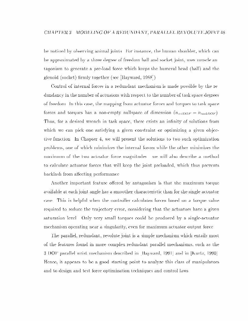
CHAPTER 3. MODELING OF AREDUNDANT, PARALLEL REVOLUTE JOINT 48
be noticed by observing animal joints. For instance, the human shoulder, which can
be approximated by a three-degree-of-freedom ball-and-socket joint, uses muscle an-
tagonism to generate a pre-load force which keeps the humeral head (ball) and the
glenoid (socket) rmly together (see [Hayward, 1988]).
Control of internal forces in a redundant mechanism is made possible by the re-
dundancy in the number of actuators with respect to the number of task space degrees
of freedom. In this case, the mapping from actuator forces and torques to task space
forces and torques has a non-empty nullspace of dimension (nactDOF ntaskDOF ).
Thus, for a desired wrench in task space, there exists an innity of solutions from
which we can pick one satisfying a given constraint or optimizing a given objec-
tive function. In Chapter 4, we will present the solutions to two such optimization
problems, one of which minimizes the internal forces while the other minimizes the
maximum of the two actuator force magnitudes. we will also describe a method
to calculate actuator forces that will keep the joint preloaded, which thus prevents
backlash from aecting performance.
Another important feature oered by antagonism is that the maximum torque
available at each joint angle has a smoother characteristic than for the single actuator
case. This is helpful when the controller calculates forces based on a torque value
required to reduce the trajectory error, considering that the actuators have a given
saturation level. Only very small torques could be produced by a single-actuator
mechanism operating near a singularity, even for maximum actuator output force.
The parallel, redundant, revolute joint is a simple mechanism which entails most
of the features found in more complex redundant parallel mechanisms, such as the
3-DOF parallel wrist mechanism described in [Hayward, 1991] and in [Kurtz, 1990].
Hence, it appears to be a good starting point to analyze this class of manipulators
and to design and test force optimization techniques and control laws.

CHAPTER 3. MODELING OF AREDUNDANT, PARALLEL REVOLUTE JOINT 49
ρ ρ
λ
λ
k k
r rγ
ψ
1
1 2
2
1
2
Joint Axis
P P
A B
1 2
= k + r
= k + r
1
2
actuator 1 actuator 2
Figure 3.3: Geometry of the Parallel Revolute Joint
3.2 Kinematics of the Parallel, Redundant, Rev-
olute Joint
In this section, the kinematics of the planar parallel revolute joint with actuator
redundancy are derived. The notation used is illustrated at Figure 3.3.

CHAPTER 3. MODELING OF AREDUNDANT, PARALLEL REVOLUTE JOINT 50
3.2.1 Inverse Kinematics
The law of cosines applied to triangles A and B yields two expressions for the actuator
lengths 1 and 2:
1 =q21 + r2 21r cos ; (3.1)
2 =q22 + r2 22r cos( ) : (3.2)
3.2.2 Direct Kinematics
Equations 3.1 and 3.2 can be inverted; they yield equations 3.3 and 3.4 for the joint
angle .
= arccos
21 + r2 21
21r
!; (3.3)
= arccos
22 + r2 22
22r
!: (3.4)
Since the joint angle may become negative or greater than the angle , the
redundancy in sensing allows us to determine its sign. Assuming that the arccos
function always gives an answer in the rst or the second quadrant (which is the case
in the c language), the idea is to check whether 1 is greater than 2, and if it is,
equation 3.3 is used to calculate . In the opposite case, equation 3.4 must be used.
This method also has the advantage of always using the best conditioned sensor to
calculate the joint angle.
3.2.3 Velocity Mapping: The Jacobian Matrix
We are now interested in calculating the time-varying linear transformation mapping
the joint angular velocity to the actuator linear velocities. We thus dene the 2x1
jacobian matrix J (or more simply the jacobian) of the mechanism by the following

CHAPTER 3. MODELING OF AREDUNDANT, PARALLEL REVOLUTE JOINT 51
relationship. 264 _1
_2
375 = J _ : (3:5)
It can be calculated by dierentiating equations 3.1 and 3.2:
_1 =1r sin
1_ ; (3.6)
_2 =2r sin( )
2_ : (3.7)
Hence,
J =
264 1r sin
1
2r sin( )2
375 : (3:8)
By using the principle of virtual work, it can be easily shown that the joint output
torque is related to the actuator forces by the tranpose of the jacobian:
= JTf ; (3:9)
where f = [f1 f2]T is the vector of forces applied by the actuators.

CHAPTER 3. MODELING OF AREDUNDANT, PARALLEL REVOLUTE JOINT 52
3.3 Autonomous Kinematic Calibration of the Rev-
olute Joint
In order to be able to calibrate the kinematic parameters of the parallel revolute joint,
most kinematic calibration methods (see for example [Whitney, Lozinski, Rourke, 1986])
would require that an external device be used to measure the joint angle with sucient
accuracy. Then a nonlinear search of the kinematic parameters could be implemented
to nd the best set of parameters satisfying the consistency equations which relate the
measured joint angle to the kinematic parameters through the geometry of the mech-
anism. Instead of using external measurements, Bennett and Hollerbach observed
in [Bennett and Hollerbach, 1991] that single-loop closed kinematic chains formed by
serial-type manipulators can be calibrated when the manipulator is redundant with
respect to the task, i.e. when it has more degrees of freedom than required to perform
the task. The key idea is to avoid the need of having external measurements of the
endpoint position or orientation by constraining some of the cartesian space degrees
of freedom to a known position or orientation and then to use redundancy in joint
sensing to eliminate the unsensed passive degrees of freedoms of the task kinematics.
These results can be directly used to calibrate the parallel revolute joint even
though it belongs to the class of parallel manipulators. The following observations
can be made on the structure of this mechanism (see Figure 3.3). First, it is composed
of two closed kinematic chains (triangles A and B), each formed by the actuator and
the moment arm, and both of which are position constrained in a plane at the joint's
rotation axis. If we put a coordinate system at that point, we then readily know that
the endpoint position of the two kinematic chains is the origin, and two loop closure
equations could be derived in the x and y coordinates for each closed kinematic chain.
The passive task degree of freedom is the joint angle , which must be eliminated
from the loop closure equations.

CHAPTER 3. MODELING OF AREDUNDANT, PARALLEL REVOLUTE JOINT 53
In fact, it is simpler not to use a coordinate system but to use only one loop
closure equation derived from triangle geometry for each closed kinematic chain. For
example, the law of cosines is applied to the two kinematic chains shown at Figure
3.3, and we get equation 3.10 for chain A and equation 3.11 for chain B.
21r cos = 21 + r2 21; (3:10)
22r cos( ) = 22 + r2 22 (3:11)
We can rewrite equation 3.11 by collecting all the terms on the left-hand side, and
we dene FB = FB(1m; 2m; 10; 20; r; k1; k2; ) as
FB = 22r cos cos + 22r sin sin 22 r2 + 22 = 0; (3:12)
where i = im + i0; i = ki + r; i = 1; 2:
The angle can be eliminated in equation 3.12 by using equation 3.10. We restrict
the analysis to the subworkspace > 0. Equation 3.15 is the loop closure equation
needed for the nonlinear iterative search. Such a method is required because the
kinematic parameters do not map linearly into FB. We see that equation 3.15 can
be scaled arbitrarily, that is, any scaled version of the mechanism will satisfy it, and
hence one of the kinematic parameters must be specied at the outset for the solution
to be unique in a small neighborhood around it.
cos =21 + r2 21
21r; (3:13)
sin =
0@1
21 + r2 21
21r
!21A1=2
; (3:14)
FB =21
cos (21 + r2 21) + 22r sin
0@1
21 + r2 21
21r
!21A1=2
22 r2 + 22:
(3:15)

CHAPTER 3. MODELING OF AREDUNDANT, PARALLEL REVOLUTE JOINT 54
The Levenberg-Marquardt algorithm is used to identify the kinematic parameters
(k1, k2, 10, 20, ) of the mechanism because it is numerically robust. This algo-
rithm is based on a linearization of the nonlinear equation and thus needs the partial
derivatives of FB with respect to each of the kinematic parameters except the moment
arm's length r which is used to scale the mechanism and is supposed to be known with
good accuracy. These partial derivatives are listed in appendix A. A large numberM
of actuator position measurements (1m; 2m) must be taken inside the subworkspace
decribed by > 0. Now dene the 5x1 jacobian matrix Ci as follows, where the
superscript i denotes the ith conguration in which the mechanism was placed to take
the ith measurement (i1m; i2m).
Ci =
"@F i
B
@k1
@F iB
@k2
@F iB
@10
@F iB
@20
@F iB
@
#: (3:16)
Let
C =
2666664C1
...
CM
3777775 ; F =
2666664F 1B
...
FMB
3777775 ; =
26666666666664
k1
k2
10
20
37777777777775; =
266666411m 12m...
...
M1m M2m
3777775 :
The explicit dependency of F on and is stressed when we write
F = F(; ): (3:17)
The rst order dierential of F with respect to is
F = C; (3:18)
In the case where C has full column rank (i.e. is one to one since M 5),
can be calculated as follows
= (CTC)1CTF: (3:19)

CHAPTER 3. MODELING OF AREDUNDANT, PARALLEL REVOLUTE JOINT 55
For a given estimate of the vector of kinematic parameters which diers from
the true vector by approximately , the dierential F can be calculated easily:
F = F F c = Fc; (3:20)
where F c = F(; ); F = F(; ) = 0 assuming is noise-free.
Given these relationships, it is possible to use a Newton-like method to search
for the optimal set of kinematic parameters, such as the aforementioned Levenberg-
Marquardt algorithm.
3.3.1 The Levenberg-Marquardt Algorithm
This iterative scheme consists of linearizing the nonlinear function F about the cur-
rent estimate of the parameters k, then calculating a correction vector
k+1of
the parameters by using a modied pseudo-inverse of the jacobian matrix C, and
then adding this correction vector to the current estimate to form the new estimate.
The algorithm iterates until, for example, the 1-norm of F gets smaller than a
pre-specied threshold. It should be noted that C and F must be evaluated at each
iteration using the current estimate k. The algorithm implemented to identify the
kinematic parameters of the parallel mechanism is outlined here.
(0) Set k to 0, and to small values. Use a reasonable rst estimate 0.
(1) Calculate Fkc (
k; ) and C(
k; ) ,
(2) Calculate the correction vector k+1
and the new estimate k+1
:
k+1
= (CkTCk + I)1CkTFkc ,
k+1
= k+
k+1.
(3) Let k = k + 1, goto (1) and iterate until kFkck1 < .
The diagonal matrix I is needed to avoid numerical singularities when the jaco-
bian matrix C loses rank, and it helps nd the desired solution even if a bad initial

CHAPTER 3. MODELING OF AREDUNDANT, PARALLEL REVOLUTE JOINT 56
estimate of the parameters is used. In a practical implementation, has to be grad-
ually reduced as the estimate approaches the solution, otherwise it will reduce the
rate of convergence of the iteration. Introduction of this diagonal matrix also corre-
sponds to minimizing the criterion kCFk2+T which penalizes large
variations in the parameters during the search.
3.3.2 Experimental Results
In simulations where the actuator position measurements were assumed to be perfect,
the kinematic parameters were quickly recovered, even for bad initial estimates. How-
ever, our rst try to estimate the kinematic parameters of the real mechanism proved
unsuccessful, even though the moment arm's length had been measured with an ac-
curacy of about 0:05 mm (r = :06374 m). We used a 12-bit A/D converter which
provided a sensitivity of about 1:78x105m, but the actuator position signals coming
from the LVDT sensors were corrupted by noise and for each static conguration we
had to average the position measurements over 100 samples. Further simulations in
which zero-mean uniformly-distributed white noise of magnitude 106 m (less than
the A/D converter sensitivity) was added to the measurements failed to nd a con-
sistent set of parameters. Hence we had to modify our scheme to deal with this level
of uncertainty in measurement.
Apart from the noisy measurements, the failure of the search was also believed
to partly result from three other possible causes. The rst one is the geometric
model which might not be consistent with the real mechanism. A second possible
explanation is that we did not use enough measurements (we usedM = 50), although
this hypothesis was quickly abandoned after the simulations had shown that using
100 measurements corrupted by the noise described above would not improve the
search. The third possible reason is that a priori xing of r might not constrain the
search to a small enough region in parameter space. Intuitively, if the sensitivity of

CHAPTER 3. MODELING OF AREDUNDANT, PARALLEL REVOLUTE JOINT 57
FB with respect to r is small, many dierent sets of parameters could reach a given
bound on the 1-norm of F c. One solution would be to accurately measure a second
parameter to which FB would be more sensitive, and then to estimate the remaining
four parameters. Even if FB is not really more sensitive to variations in the second
xed parameter, the search should be better constrained in the neighborhood of the
optimal solution because of the fact that there are now two xed parameters which
reduce uncertainty in the estimate of the others.
Not much could be done to improve the kinematic model so it was decided to
investigate the third possible cause. We xed k2 because 2 could be easily measured
and it was believed that FB was sensitive enough to it. This does not restrict the
usefulness of the autonomous kinematic calibration method because the hardest pa-
rameters to measure are the actuator dead lengths 10 and 20 and the angle . The
jacobian matrix Ci and the vector of unknown kinematic parameters have to be
redened as follows.
Ci =
"@F i
B
@k1
@F iB
@10
@F iB
@20
@F iB
@
#; (3:21)
=
2666666664
k1
10
20
3777777775: (3:22)
With these new denitions and the same denitions of C, F and as before, the
Levenberg-Marquardt algorithm outlined above can be used directly to estimate the
kinematic parameters. The actual algorithm implemented on matlabTM is presented
in appendix B. Simulations were run with the same noisy measurement matrix as
described above, i.e. with a zero-mean uniformly-distributed white noise between
106 m, and the parameters were recovered to within about .25 mm and 105 rad.
Simulations with noise of maximum amplitude 105 m produced estimates which had
one length parameter o by as much as 1 mm, but the angle was recovered with an

CHAPTER 3. MODELING OF AREDUNDANT, PARALLEL REVOLUTE JOINT 58
accuracy of 104 rad. Since an A/D converter with more than 12 bits of resolution
was not available at that time, we tried to estimate the kinematic parameters of the
real mechanism using the 12-bit converter.
Before we could use the autonomous calibration scheme for the real mechanism,
we had to accurately measure 2. It was measured to be 28:66 :05 cm, thus the
parameter k2 = 2 r is k2 = 22:29 :05 cm. The kinematic parameters of the
redundant, parallel revolute joint were successfully identied starting from two very
dierent initial estimates. The lengths appeared to be exact to within about 1 mm,
and the angle was identied to within about :001 rad. These results are somewhat
satisfying considering the simulation results with a noise level comparable to the
quantization eect. The kinematic parameters are shown at Table 3.1.
k1 22.30 cmk2 (measured) 22.29 cmr (measured) 6.374 cm10 22.09 cm20 22.04 cm .633 rad
Table 3.1: Calibrated Kinematic Parameters of the Parallel Revolute Joint

Chapter 4
Optimization of the Joint's
Actuator Forces
4.1 Actuator Forces to Joint Torque Mapping:
The Transposed Jacobian
The joint output torque is related to the actuator forces by the tranpose of the
jacobian:
= JTf ; (4:1)
where 2 R, JT = [j1 j2] 2 R2, f = [f1 f2]T 2 R2:
Equation 4.1 can be explicitly written as:
=
"1r sin
1
2r sin( )
2
#f : (4:2)
59

CHAPTER 4. OPTIMIZATION OF THE JOINT'S ACTUATOR FORCES 60
4.2 Optimization of Actuator Forces Seen as a
Minimum-Norm Problem
An innity of solutions exists for the vector of actuator forces in equation 4.1, and we
shall present two methods for nding the minimum-norm optimal solution according
to two dierent denitions of the norm, one in Hilbert space, the other in a Banach
space.
The rst optimization problem may be stated as follows: given the relationship
between and f , nd the optimal minimum-norm vector ~f that satises it when the
norm is chosen to be the usual Hilbert space norm:
kfk = (f21 + f22 )1=2: (4:3)
The second minimumnorm optimization problem is formulated in a Banach space
with a norm dened as
kfk1 = max(jf1j; jf2j): (4:4)
Both methods lead to very simple solutions which can be calculated in real time.
The 2-norm optimal vector produces a resultant force which is orthogonal to the
moment arm, the latter being aligned with the nullspace of the transposed jacobian, so
that this resultant force delivered by the actuators contributes entirely to the torque
applied at the joint. It also comes from a linear transformation applied to the desired
joint torque and is thus easy to calculate even for systems having more degrees of
freedom.
The 1-norm optimal solution minimizes the maximum absolute value of the ac-
tuator forces at any time and can therefore be regarded as a way to reduce stress
on the force sensors. It also enables the system to reach higher output torques given
the force limits of the actuators because as will be seen below, the 1-norm solution
vector has forces that are equal in magnitude, and that magnitude is minimal. On

CHAPTER 4. OPTIMIZATION OF THE JOINT'S ACTUATOR FORCES 61
the other hand, a high output force may be applied on one of the actuators that is, or
close to being, singular, which is not the case for the 2-norm optimal solution which
always makes an actuator close to, or at, a singularity very compliant.
4.2.1 Minimum 2-norm Optimal Vector of Forces
The minimum 2-norm optimal vector of actuator forces corresponds to the solution
of equation 4.1 obtained by using the pseudo-inverse of the transposed jacobian JT
which is an onto transformation. The optimal vector is simply
~f = J(JTJ)1; (4:5)
which turns out to be
~f =
j21 + j22
264 j1
j2
375 : (4:6)
This expression would be the most ecient one in an actual implementation pro-
vided the jacobian has already been computed. A more explicit expression of ~f is
now given in terms of the kinematic parameters:
~f =12
r(2122 sin
2 + 2221 sin
2( ))
264 21 sin
12 sin( )
375 : (4:7)
It is interesting to note that when an actuator aligns with the moment arm, for
example actuator 1 when = 0, the force it applies is 0 since sin(0) = 0. Therefore
actuator 1 becomes very compliant around = 0.
4.2.2 Minimum1-norm Optimal Vector of Forces
The optimization problem is stated as follows: given a torque , is there a minimum-
norm vector ~f satisfying equation 4.1 when the norm is dened as in equation 4.4
above, and if so, can we nd its expression? We use the theory of dual Banach

CHAPTER 4. OPTIMIZATION OF THE JOINT'S ACTUATOR FORCES 62
spaces as presented in [Luenberger, 1969] to solve this problem. Roughly speaking,
the dual space of linear functionals of a normed space plays a role analogous to the
inner product in Hilbert space and with careful interpretation, the projection theorem
which gives the solution to minimum-norm problems in Hilbert space can be extended
to arbitrary Banach spaces.
First, recall that lp spaces are spaces of innite sequences of real numbers with
norm dened as
kxkp = +1Xi=1
jxijp!1=p
; (4:8)
where x 2 lp, x = fx1; x2; x3; : : :g, xi; p 2 R, 1 p < +1:
For p = +1, the l1 space is the space of bounded sequences of real numbers, and
the norm is dened as
kxk1 = supijxij: (4:9)
Our purpose will be to use a subspace of l1 in which vectors have only their rst
two elements not identically zero, and also a subspace of l1 dened similarly. Also
needed is the following denition of a normed dual space.
Denition 1 Let X be a normed linear vector space. The space of all bounded linear
functionals on X is called the normed dual of X and is denoted as X . The norm of
an element x 2 X is dened as
kxk = supkxk1
jx(x)j; (4:10)
where x(x) denotes the value of the linear functional x at x 2 X .
The value of x at x 2 X will also be denoted by hx; xi or by hx; xi to suggestthe analogy with the inner product in Hilbert space. It can be shown that the
space X is a Banach space, i.e. a complete normed linear space. For the special
case where X is the lp space, it can also be shown that the normed dual of X is lq

CHAPTER 4. OPTIMIZATION OF THE JOINT'S ACTUATOR FORCES 63
where1=q + 1=p = 1. In that case, all bounded linear functionals x 2 X lq can
be expressed as
hx; xi =+1Xi=1
ii; (4:11)
where x = f1; 2; 3; : : :g 2 lp, f1; 2; 3; : : :g = y 2 lq, i; i 2 R:
We say that X is equivalent to lq in the sense that there is a one to one corre-
spondence between the sequence y = f1; 2; 3; : : :g 2 lq and the linear functional
in equation 4.11, and every element of lq denes a member of X . From now on,
vectors in the dual space X of an lp space will be referred to as x 2 X or as y 2 lq,depending on the context.
We are now ready to show that the normed dual space X of the space X of pairs
of real numbers x = (1; 2) with norm dened as kxk1 =P2i=1 jij is the space of
pairs of real numbers y = (1; 2) with norm dened as in equation 4.4.
Proposition 1 The normed dual space X of the space X of all pairs of real numbers
with norm dened as
kxk1 =2Xi=1
jij; (4:12)
where x = (1; 2) 2 X ;
is the space of all pairs of real numbers y = (1; 2) with norm dened as
kxk = kyk1 = maxi=1;2
jij: (4:13)
Moreover, the value of x at x can be expressed as
hx; xi =2Xi=1
ii: (4:14)
Proof: First, we consider a subspace V1 of l1 consisting of all sequences of the
form v = f1; 2; 0; 0; 0; : : :g where 1; 2 2 R, and a subspace W1 of l1 consisting of
all sequences of the form w = f1; 2; 0; 0; 0; : : :g where 1; 2 2 R. We see that

CHAPTER 4. OPTIMIZATION OF THE JOINT'S ACTUATOR FORCES 64
V1 and W1 are only extensions of X and X obtained by padding zeros to get
innite sequences. We know that the dual space of l1 is l1 from [Luenberger, 1969].
Therefore, it is clear that the dual space of W1 is V1, and that all bounded linear
functionals of V1 can be written as
hw; wi = hv; wi =+1Xi=1
ii =2Xi=1
ii: (4:15)
The norm of w is
kwk = kvk1 = maxi=1;2;:::
jij = maxi=1;2
jij: (4:16)
Since the summation in equation 4.15 runs from i = 1 to 2, and the norms of W1
and V1 use only the rst two elements of the sequences, it is readily seen that the
zero padding is not necessary for equations 4.15 and 4.16 to hold. Hence X is the
normed dual space of X with norm dened as in equation 4.13.
Q.E.D.
The 1x2 transposed jacobian JT in equation 4.1 will be regarded as an element of
X while f will be considered as belonging to X . Equation 4.1 can be rewritten as
hf; JT i = : (4:17)
Now the problem is: nd an f 2 X such that equation 4.17 is satised and kfk1is minimum, or, in other words, nd an element f of the coset K dened by equation
4.17 such that its norm is minimum. Since we have formulated the optimization
problem in a dual space, the minimum-norm vector is guaranteed to exist by virtue
of theorem 2, Section 5.8 of [Luenberger, 1969], which we have adapted to the problem
at hand and present here as Theorem 1. But before, we need the following denitions
of alignment and orthogonality properties in dual spaces.
Denition 2 A vector x 2 X is said to be aligned with a vector x 2 X if
hx; xi = kxkkxk.

CHAPTER 4. OPTIMIZATION OF THE JOINT'S ACTUATOR FORCES 65
Denition 3 The vectors x 2 X and x 2 X are said to be orthogonal if hx; xi = 0.
Denition 4 Let U be a subset of a normed linear space X . The orthogonal comple-
ment of U , denoted U?, consists of all elements x 2 X orthogonal to every vector
in U .
Theorem 1 Let M denote the one-dimensional subspace generated by JT 2 X , and
let f be a vector in X . Then,
d = minhf;JT i=
kfk = minm2M?
kf mk = supx2M;kxk1
hx; fi; (4:18)
where f satises hf ;JT i = , and the minimum is achieved for some m0 2 M?. If
the supremum on the right is achieved for some x0 2 M, then f m0 is aligned with
x0.
The proof can be found in [Luenberger, 1969]. Corollary 1 of Theorem 2 in Section
5.8 of the same reference is also useful and we state it here as Corollary 1 adapted to
our Theorem 1.
Corollary 1
d = minhf;JT i=
kfk = maxkaJT k11
hf ; aJT i = maxkaJT k11
a; (4:19)
where f satises hf ;JT i = and a 2 R:
Furthermore, the optimal vector ~f is aligned with the optimal aJT , i.e.
h~f ; aJT i = k~fk1kaJTk1: (4:20)
This immediately follows once we notice that the subspace M can be described
by aJT , a 2 R. If we explicitly write the norms in equation 4.20, we get
h~f ; aJT i = jaj2X
k=1
jjkjmaxi=1;2
j~fij; (4:21)

CHAPTER 4. OPTIMIZATION OF THE JOINT'S ACTUATOR FORCES 66
but
h~f ; aJT i = a2Xi=1
ji ~fi = a: (4:22)
Hence,
maxi=1;2
j~fij2X
k=1
jajjjkj =2Xi=1
aji ~fi: (4:23)
This occurs only when the following conditions are met:
(i) j ~f1j = j ~f2j = k~fk1(ii) sign( ~fi) = sign(aji); i = 1; 2
Also, since
d = minhf;JT i=
kfk = k~fk1 = maxi=1;2
j~fij; (4:24)
it follows that
j~fij = maxkaJT k11
a , i = 1; 2: (4:25)
For a complete characterization of the optimal vector ~f , we need to nd maxkaJT k1 a .
We maximize a under the constraint
2Xi=1
jajjjij 1; (4:26)
jaj 1P2i=1 jjij
: (4:27)
Hence,
a =sign( )P2i=1 jjij
(4:28)
maximizes a . Then, from condition (i) above,
k~fk1 = j ~f1j = j ~f2j = a =j jP2i=1 jjij
: (4:29)
Finally, using condition (ii), the optimal vector of forces ~f is
~f =
jj1j+ jj2j
264 sign(j1)
sign(j2)
375 ; (4:30)

CHAPTER 4. OPTIMIZATION OF THE JOINT'S ACTUATOR FORCES 67
where sign() =
8><>:1 , < 0
+1 , 0; 2 R:
We see that its expression is very simple and can be easily computed in real time.
4.2.3 Addition of a Pre-Load Force on the Joint
It may be desirable to apply a small pre-load force in a joint in order to reduce the
eect of a loosened bushing or bearing. It can be accomplished by using a force vector
lying in the nullspace of JT . Such a vector would be aligned with the moment arm
and thus would not contribute to the movement of the joint. Let n be a unit vector
lying in N (JT ) and pointing outward from the joint axis. It can be expressed as
n =
8><>:
[j2(j21 + j22)1=2 (1 + j22=j
21 )1=2]T ; > 0
[(1 + j21=j22)1=2 (1 + j22=j
21)1=2]T ; 0
: (4:31)
A pre-load force of Fpl newtons will be applied on the joint if a force vector Fpln is
added to the 2-norm optimal vector ~f corresponding to a desired torque . It should
be noted that the 1-norm optimal vector of forces cannot be used for that purpose.

Chapter 5
Control of the Redundant Parallel
Joint
In robotics, it is necessary for a controller to perform reasonably well under many
circumstances because the inertial parameters and friction eects may vary in large
proportions when a manipulator moves, picks up a load, makes contact with the
environment, etc. This is especially true for hydraulic robots since they can handle
heavy payloads, in which case their inertial parameters undergo large variations.
Hence a good controller should be able to either adapt itself to these changes or at
least guarantee that the system will remain stable at all times while maintaining a
certain desired performance level. This latter property is referred to as the robustness
of a control system as discussed in Chapter 1. The aim of this chapter is to compare
three linear, time-invariant position controllers for the parallel joint, and not to nd
the best controller possible. Thus the class of adaptive controllers is deliberately
excluded at the outset because it is believed that uncertainty in the system should
be taken care of in the design stage, not while the system is operating. Furthermore,
linear time-invariant control systems are much simpler and easier to analyze than are
time-varying control systems.
68

CHAPTER 5. CONTROL OF THE REDUNDANT PARALLEL JOINT 69
Two approaches are investigated for the robust position control of the revolute
joint. These approaches consist of applying linear control schemes to the system.
Linearization of the plant's dynamics is often performed by feeding back the nonlinear
dynamic terms in complex robotic systems, although here we deal with a plant that
is essentially linear if we neglect friction. Unmodeled nonlinearities, disturbances and
variations in system parameters form the uncertainty, and the robustness properties of
the two control laws should reduce its eect. A simple PD controller is rst designed
for purpose of comparison.
5.1 Dynamics of the Revolute Joint
We consider the case where the redundant revolute joint is carrying an inertial load
with unmodeled friction which is seen as a disturbance:
= I + f ; (5:1)
where I is the joint inertia and f is the friction torque.
5.2 Position Control
5.2.1 A Simple PD Controller
The problem of designing a simple position controller is straightforward for the pure-
inertia case under study. We propose the following linear proportional-derivative
(PD) control law:
= Kp( des ) +Kd( _ des _ ): (5:2)
The joint angle can not be measured directly|the direct kinematics must be
solved rst. Taking the Laplace transforms of both sides of (5.1) and (5.2) and

CHAPTER 5. CONTROL OF THE REDUNDANT PARALLEL JOINT 70
equating them, we get
I (s)s2 +Kd (s)s+Kp (s) = Kd des(s)s+Kp des(s) f (s); (5:3)
(s)
des(s)=
Kp +Kds
Is2 +Kds+Kp: (5:4)
Equation 5.4 is the closed-loop transfer function from the desired angle des to
the actual angle . If the desired trajectory is specied not only by the angle but
also by its rst two derivatives, the desired angular acceleration can then be used as
a feedforward term. Also, multiplying the control by an estimate of the inertia I will
make the resulting closed-loop second-order system behave as if it had a unit inertia:
= I( des +Kp( des ) +Kd( _ des _ )): (5:5)
This control law corresponds to the computed torque method [Paul, 1972].
Using (5.1) and (5.5), and letting I = I,
( des ) +Kd( _ des _ ) +Kp( des ) = f : (5:6)
With e = des , equation 5.6 can be written as:
e+Kd _e+Kpe = f : (5:7)
This is the error equation, and if f is identically zero or an impulse, e will tend to
zero at a rate governed by the values of Kp and Kd. However, in a real system, the
friction torque may be a persisting disturbance (e.g. stiction), and in that case the
error will not be null in steady-state. In the next section, we develop a robust PID
controller which can drive the error to zero even in the presence of a constant torque
disturbance.
A block diagram of the PD controller is shown in Figure 5.1. The controller
calculates a control torque but the inputs to the system are desired actuator forces as

CHAPTER 5. CONTROL OF THE REDUNDANT PARALLEL JOINT 71
γ
γ
γ
τ
ρ
ρ+
+ +
−+
−+
KK
IJoint and Actuator
DynamicsForce
Optimizer
f
Kinematics
γ
γ
(J J) JT −1 T
d
d
d
dp
^ −
−
−
es
es
es K( )
Figure 5.1: Block Diagram of the PD Controller
discussed in Chapter 4. Thus, if we use the 2-norm optimal solution for the actuator
forces, the control law can be expressed as:
~f =( des +Kp( des ) +Kd( _ des _ ))I12
r(2122 sin
2 + 2221 sin
2( ))
264 21 sin
12 sin( )
375 : (5:8)
The feedback gains Kp and Kd can be chosen based on desired natural undamped
frequency and damping factor. A reasonable choice would be an undamped natural
frequency !n = 25 rad/s (corresponding to 4 Hz) and a damping factor = :71. Thus
Kp = !2n = 632; (5:9)
Kd = 2!n = 35:7: (5:10)
The Bode plot of the cascaded plant and controller is shown in Figure 5.2.

CHAPTER 5. CONTROL OF THE REDUNDANT PARALLEL JOINT 72
-50
0
50
100
100 101 102 103 104
Frequency (rad/sec)
Gai
n dB
-180
-160
-140
-120
-100
-80
100 101 102 103 104
Frequency (rad/sec)
Phas
e de
g
Figure 5.2: Bode Plot of the Cascaded PD Controller and Plant (Open-Loop)
τ γ γ
γ
w
n
γ1__
I s2
m
d
(disturbance)
(noise)
C(s)−es + +
+
+
Figure 5.3: Block Diagram of the Closed-Loop Robust Control System

CHAPTER 5. CONTROL OF THE REDUNDANT PARALLEL JOINT 73
5.2.2 A Robust State Feedback Controller Based on the
Internal Model Principle
The closed-loop system is shown in Figure 5.3. We will assume that we have only an
estimate of the joint's inertia I denoted as I. The goal is that the system be able
to track the reference input des(t) and to reject a possibly persistent disturbance w
in the face of uncertainty in the knowledge of the system's inertia and measurement
noise. This is known as the robust servomechanism problem.
Theory
The rst method we use is based on the Internal Model Principle of control theory
[Francis and Wonham, 1976]. This principle states that a regulator synthesis (i.e.
the whole closed-loop system) is structurally stable only if the controller utilizes
feedback of the regulated variable, and incorporates in the feedback path a suitably
reduplicated model of the dynamic structure of the exogeneous signals which the
regulator is required to process. A system is said to be structurally stable if it remains
stable for slight variations in its state-space model parameters.
Although this principle is important in theory, it has a major drawback in practice:
it is impossible to have a priori knowledge of the eect of uncertainty and disturbance.
In fact, these may well be stochastic signals. Hence, attempting to build an inter-
nal model of a disturbance may have limited success in that context. Nevertheless,
[Kuo and Wang, 1991] demonstrated the usefulness of the method when the uncer-
tainty, which combines the eect of uncertainty in the robot's dynamic model and a
disturbance at the output, is assumed to be constant ( _e = 0) but of unknown magni-
tude. In this case, the resulting controller is just a classical PID controller, that is, an
integral term is added to the usual state feedback controller. This fact was pointed
out in [Desa and Roth, 1985].

CHAPTER 5. CONTROL OF THE REDUNDANT PARALLEL JOINT 74
The approach taken by Kuo and Wang is as follows. First decouple and linearize
the system, making it second-order in each decoupled direction in task space by a
proper choice of feedback gains Kp and Kd. Then apply the robust linear control
on the linearized system, which amounts to adding an integrator on the error in the
feedback when a constant disturbance model is used.
The internal model approach is attractive because it is possible to set the rate at
which the error will be driven to zero by selecting the poles of a linear subsystem.
We lose this advantage if we only merely try to put integrators with gains in the
compensator. Here, we follow the approach taken by Kuo and Wang to design a
PID controller for our simple system, i.e. we will assume that the uncertainty signal
combining the uncertainty in the plant's parameters and disturbance is a constant.
Referring to Figure 5.3 for the notation, we rst apply a state feedback to equation
5.1,
I = I(Kd _ m Kp m +Kpu); (5:11)
where u is a linear input.
The reference trajectory is known and we dene ud with the following equation:
Kpud = des +Kd _ des +Kp des: (5:12)
Now by subtracting equation 5.12 from equation 5.11, we get
Kp(u ud) =I
I des +Kd( _ m _ des) +Kp( m des): (5:13)
Dene y = des as the tracking error and v = uud as the input from the robust
part of the controller. Also, let I = I +I. We have
Kpv = y I
Iw +
I
I +Kd( _ + _n _ des) +Kp( + n des); (5:14)
Kpv = y +Kd _y +KpyIIw +
I
I +Kd _n+Kpn| z e
; (5:15)

CHAPTER 5. CONTROL OF THE REDUNDANT PARALLEL JOINT 75
y +Kd _y +Kpy = Kpv e: (5:16)
The uncertainty is
e = Kd _n+Kpn I
Iw +
I
I : (5:17)
Equation 5.17 tells us that for a small I and low-power noise, a slowly-varying e
implies that the disturbance w is also slowly-varying, since w must have its energy at
low frequency. The assumption that e be constant may be justied for slowly-varying
disturbances as well, which for example may be due to friction. In other words,
integral control works also well for slowly-varying uncertainty. Equation 5.16 can be
rewritten in state-space form.
Let x =
264 y
_y
375 : Then,
_x =
264 0 1
Kp Kd
375
| z A
x+
264 0
Kp
375
| z B1
v +
264 0
1
375
| z B2
e; (5:18)
y = [1 0]| z C
x: (5:19)
We dene the following quantities:
z = _x; (5:20)
s = _v: (5:21)
Take the vector z to be a new state vector, and s to be a new input. Dierentiating
(5.20) and using (5.19) and (5.21) yields
_z = A _x+B1 _v +B2 _e| z 0
; (5:22)
_z = Az + B1s; (5:23)

CHAPTER 5. CONTROL OF THE REDUNDANT PARALLEL JOINT 76
_y = Cz: (5:24)
Now, let be a new state vector formed as follows:
=
2666664y
_y
y
3777775 =
264 y
z
375 : (5:25)
The following state and output equations can be obtained:
_ =
26666640 1 0
0 0 1
0 Kp Kd
3777775
| z G
+
2666664
0
0
Kp
3777775
| z H
s; (5:26)
y = [1 0 0]| z F
: (5:27)
The output of this system, y, is what we want to drive to zero at a desired rate.
We now show that this system is controllable. We form the controllability matrix C
and verify that it has full rank.
C = [H GH G2H]; (5:28)
C =
2666664
0 0 Kp
0 Kp KdKp
Kp KdKp K2dKp K2
p
3777775 : (5:29)
Since C is lower triangular with nonzero entries in the diagonal, it has full rank, and
thus the system is controllable. Hence we can apply a state feedback to select the
closed-loop poles at will, thereby specifying the rate at which y will be reduced to 0.
Let the gain matrix be [K1 K2 K3]. Then
s = K1y K2 _y K3y: (5:30)

CHAPTER 5. CONTROL OF THE REDUNDANT PARALLEL JOINT 77
But
v =Z t
0s()d = K1
Z t
0y()d K2y K3 _y: (5:31)
We see that v represents a PID control input. The overall control is
u = K1
Z t
0y()d K2y K3 _y +
1
Kp des +
Kd
Kp_ des + des; (5:32)
= I[Kd _ m Kp m + des +Kd _ des +Kp des KpK2( des)
KpK3( _ _ des)KpK1
Z t
0( () des())d]: (5.33)
Since and _ are unknown, we use their measurement m and _ m in the control
signal . Collecting the gains together, we nd the familiar PID control law plus a
feedforward term
= I[ des + ~Kp( des m) + ~Kd( _ des _ m) + ~Ki
Z t
0( des() m())d]; (5:34)
where ~Kp = Kp +KpK2;
~Kd = Kd +KpK3;
~Ki = KpK1:
Controller Design
We now procede to compute the controller parameters for the real system. The
principal guideline is to keep the poles of the robust part to the left of the ones
introduced for the mass-spring-damper part. The system dynamics are described by
equation 5.1, and we rst apply a PD controller to this system as shown in Figure
5.4.
We pick Kp=25.3 and Kd=7.14 such that the undamped natural frequency is .8
Hz and the damping factor is = :71, the latter so chosen as to obtain a maximally
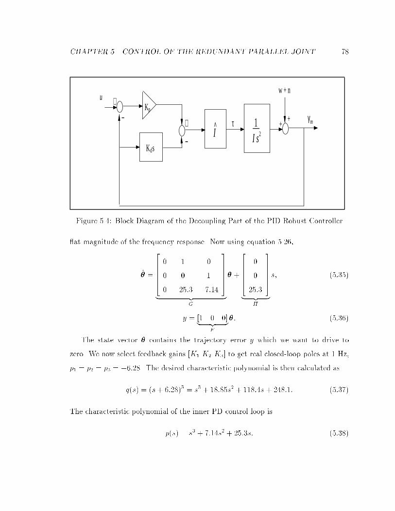
CHAPTER 5. CONTROL OF THE REDUNDANT PARALLEL JOINT 78
K s
K
1__
u
I I s
p
d
2
γτ
+
− +
−
^ m
w + n
++
Figure 5.4: Block Diagram of the Decoupling Part of the PID Robust Controller
at magnitude of the frequency response. Now using equation 5.26,
_ =
26666640 1 0
0 0 1
0 25:3 7:14
3777775
| z G
+
2666664
0
0
25:3
3777775
| z H
s; (5:35)
y = [1 0 0]| z F
: (5:36)
The state vector contains the trajectory error y which we want to drive to
zero. We now select feedback gains [K1 K2 K3] to get real closed-loop poles at 1 Hz,
p1 = p2 = p3 = 6:28. The desired characteristic polynomial is then calculated as
q(s) = (s+ 6:28)3 = s3 + 18:85s2 + 118:4s + 248:1: (5:37)
The characteristic polynomial of the inner PD control loop is
p(s) = s3 + 7:14s2 + 25:3s: (5:38)

CHAPTER 5. CONTROL OF THE REDUNDANT PARALLEL JOINT 79
yyyyvK
K
K
K
K
K
p
d
p
1
2
3
−
−−
+
−−
ud +
s s s1 1 1’’’
Figure 5.5: State Space Diagram of the PID Robust Control System
By referring to Figure 5.5, we see that the feedback gains must be picked such
that
K1Kp = 248:1;
K2Kp = 118:4 25:27 = 93:13;
K3Kp = 18:85 7:14 = 11:71:
And nally, the PID gains are computed
~Kp = Kp +KpK2 = 25:27 + 93:13 = 118:4;
~Kd = Kd +KpK3 = 7:14 + 11:71 = 18:85;
~Ki = KpK1 = 248:1:
Note that the resulting PID gains are equal to the coecients of the desired
characteristic polynomial in this case. The control is given by
= I[ des+118:4( des m)+18:85( _ des _ m)+248:1Z t
0( des() m())d]: (5:39)
The Bode plot of the cascaded plant and controller is shown in Figure 5.6 while the

CHAPTER 5. CONTROL OF THE REDUNDANT PARALLEL JOINT 80
-50
0
50
100
150
10-1 100 101 102
Gai
n dB
Frequency (rad/sec)
Bode Plot of C(s)G(s), Kp=118.4 Kd=18.85 Ki=248.1
-300
-250
-200
-150
-100
-50
10-1 100 101 102
Frequency (rad/sec)
Phas
e (d
eg)
Figure 5.6: Bode Plot of the Cascaded PID Controller and Plant (Open-Loop)
Nyquist plot is shown in Figure 5.7. From the latter gure, it is not possible to con-
clude that the system is stable because it does not show the loops at innity, but the lo-
cus actually crosses the real axis twice clockwise to the left of the critical point (at -1)
and hence the system is stable (see [Vidyasagar, Bertschmann and Sallaberger, 1988]).
The gain margin is about -18 dB while the phase margin is close to 70. Therefore
the system should show robustness against unmodeled phase lag but not in the face
of uncertainty in the joint's inertia, especially if it is underestimated.
5.2.3 An H1-Optimal Robust Controller
Theory
The second method investigated for the robust position control of the revolute joint
is the H1 sensitivity minimization method which originated in the work of Zames in

CHAPTER 5. CONTROL OF THE REDUNDANT PARALLEL JOINT 81
-25
-20
-15
-10
-5
0
5
10
15
20
25
-30 -25 -20 -15 -10 -5 0
Real Axis
Imag
Axi
s
Nyquist Plot of Cascaded PID Controller and Plant
Figure 5.7: Nyquist Plot of the Cascaded PID Controller and Plant (Open-Loop)
[Zames, 1981]. The problem is the following: given a single-input, single-output linear
time-invariant plant aected by external disturbances and of which we have only an
approximate model, can we design a controller such that the maximum value of the
weighted sensitivity of the closed-loop system on the j!-axis is minimized? This
corresponds to a minimax problem of the sensitivity function which is the transfer
function from the eect of perturbations in plant's parameters and disturbance to the
output. A block diagram of the closed-loop system where the disturbance is taken to
be the main input is shown in Figure 5.8. The transfer function from w to is easily
calculated to be:
Hw(s) =1
1 + C(s)G(s): (5:40)
The transfer function from the input des to the output is simply
H(s) =C(s)G(s)
1 + C(s)G(s): (5:41)

CHAPTER 5. CONTROL OF THE REDUNDANT PARALLEL JOINT 82
G(s) C(s)
γ
γ
w
n
dτ
+
++ +
−
+
γ−
es
Figure 5.8: Block Diagram of the H1-Optimal Control System
Now the sensitivity S(s) is dened as follows:
S(s) =@H(s)=H(s)
@G(s)=G(s): (5:42)
and carrying out the calculations we nd
S(s) =1
1 + C(s)G(s); (5:43)
which is identical to Hw(s). Thus we see that minimizing the weighted sensitivity has
two advantages: it desensitizes the system from variations in the plant's parameters
and it attenuates the eect of the disturbance (see [Zames and Francis, 1983]).
The H1 method often leads to a conservative design in terms of tracking perfor-
mance since it is the solution to a worst-case problem. Nevertheless, the controller
will guarantee great robustness as long as the disturbance aecting the system lies in
the L2 space, i.e. if w(t) is a nite-energy signal.
In our previous design, we assumed that the eect of uncertainty and disturbance
was a constant signal although we recognized the fact that the resulting PID controller
works also well for slowly-varying disturbances. Here we have to assume that the

CHAPTER 5. CONTROL OF THE REDUNDANT PARALLEL JOINT 83
disturbance is varying but eventually dies out. This is not so bad an assumption if
we consider that the revolute joint is programmed to follow a trajectory and then
stops, which is often the case in robotics. Then the disturbance would come mainly
from dynamic eects like viscous friction in the bearings or other unmodeled dynamics
while the joint follows its trajectory.
It is important to note that an H1-optimal compensator is often not practical if
the weighting function is not chosen carefully, because it might not take into account
the limitations imposed by the actuator dynamics and the sensor noise. For example,
anH1 design sometimes results in a closed-loop magnitude that does not go to zero as
! tends to innity, thereby demanding an enormous amount of power to be delivered
at high frequencies. Nevertheless, an H1-optimal design can be a good starting point
if the weighting function is chosen carefully and if the high frequency behavior can
be xed without disturbing too much the sensitivity function in the passband.
First of all, let us recall the so-called interpolation conditions that are required for
internal stability of the closed-loop system, assuming that the compensator C(s) and
the plantG(s) are represented by minimal realizations. These interpolation conditions
are directly derived from the internal stability conditions stating that S(s), G(s)S(s)
and H(s)=G(s) must all be stable, and they must be satised when G(s) has poles
or zeros in the closed right-half plane.

CHAPTER 5. CONTROL OF THE REDUNDANT PARALLEL JOINT 84
condition 1:
If G(s) has a closed right-half plane pole of multiplicity m at p0, S(s) must have a
zero of same multiplicity at the same location.
S(p0) =dS(s)
ds
s=p0
=d2S(s)
ds2
s=p0
= : : : =dm1S(s)
dsm1
s=p0
= 0: (5:44)
condition 2:
If G(s) has a closed right-half plane zero of multiplicitym at z0, then S(s) must equal
one at that point, and the (m 1) rst derivatives of S(s) evaluated at z0 must be
zero.
S(z0) = 1; (5:45)
diS(s)
dsi
s=z0
= 0; i = 1; : : : ;m 1: (5:46)
For a plant with no closed right-half plane poles and zeros, the design of the
compensator is as follows: pick a desirable sensitivity function (or, equivalently, a
closed-loop transfer function) and calculate the controller from
C(s) =H(s)
S(s)G(s): (5:47)
If we assume that we have perfect actuators and perfect sensors, we see that we
have total freedom over the choice of S(s) (or H(s)). For example, we could use an
H1-optimal sensitivity function corresponding to a certain weighting function W (s)
which will be described later. For the case where G(s) has closed right-half plane
poles or zeros, the interpolation conditions pose constraints on the choice of S(s).
Now assume we pick a minimum-phase, proper, rational weighting function W (s)
and we seek to minimize the H1 norm of the weighted sensitivity S(s)W (s):
minimize = kSWk1 = sup!jS(j!)W (j!)j: (5:48)
We have to use a weighting function because for a strictly proper plant G(s), the H1
norm of the sensitivity is always greater or equal to 1 (see [Zames and Francis, 1983])

CHAPTER 5. CONTROL OF THE REDUNDANT PARALLEL JOINT 85
as we now show.
lim!!1
S(j!) = 1 lim!!1
G(j!)
"C(j!)
1 + C(j!)G(j!)
#= 1; (5:49)
since G(s) is strictly proper and C(s)=(1 + C(s)G(s)) is proper. Therefore
kSk1 1: (5:50)
By using a weighting function, we can make jS(j!)j small at the frequency bands
of interest by choosing a large jW (j!)j at those frequencies. This fact comes from
the nature of the optimal weighted sensitivity which is a Blaschke product:
S(s)W (s) = kBG(s) B(s): (5:51)
This result is derived from functional analysis. The Blaschke product BG(s) is formed
with the open RHP poles of G(s). Suppose these poles are denoted as pi, i = 1; : : : ; r,
then BG(s) is
BG(s) =rYi=1
s+ pis+ pi
: (5:52)
Note that BG(s), like any Blaschke product, is stable and all-pass, i.e. jBG(j!)j = 1.
The Blaschke product B(s) is needed only if the plant has RHP zeros which is not
the case for the revolute joint. Therefore, B(s) = 1 for our purposes and the constant
k can be made as small as desired.
It should be noted that the product S(s)W (s) is in H1 even though W (s) does
not necessarily belong to this space. The restriction is, if G(s) has poles on the
j!-axis, W (s) must have these poles with at least the same multiplicity; this is just
a restatement of the rst interpolation condition when equation 5.51 holds: S(s)
is required to have cancelling zeros for these poles but since the magnitude of the
Blaschke product in the right-hand side of (5.51) is 1 on the j!-axis, W (s) must be
innite at those points. This guarantees that the product S(s)W (s) belongs to H1
as long as the weighting function W (s) is not allowed to have poles or zeros in the
open right-half plane.

CHAPTER 5. CONTROL OF THE REDUNDANT PARALLEL JOINT 86
Controller Design
Now we are ready to design a desirable optimal sensitivity function by picking a
suitable weightingW (s). First we notice that jW (j!)j inverts jS(j!)j and that W (s)
must have two poles at s = 0 since the plant model is G(s) = 1=Is2. We also observe
that BG(s) = 1 because G(s) has no open RHP poles. Hence S(s) = k=W (s), so
that the sensitivity is just the inverse of the weighting function. Knowing this and
recalling that the closed-loop transfer function possess the same poles as the sensitivity
function, reasonable zeros are selected for W (s) which become the closed-loop poles.
Finally, after a few trials, we chose W (s) to be:
W (s) =(s=!a + 1)3
s2(s=b+ 1): (5:53)
The magnitude of this weighting function is plotted in Figure 5.9. The corre-
sponding optimal sensitivity is
S(s) =ks2(s=b+ 1)
(s=!a + 1)3: (5:54)
The gain k is now adjusted such that S(j!) ! 1 as ! ! 1 to make sure that
jH(j!)j rolls o at high frequencies as fast as the second order plant. Thus the
actuators will not be delivering too much power at high frequencies.
S(j!) =k!2(j!=b + 1)
(j!=!a + 1)3; (5:55)
lim!!1
S(j!) =k!3
a
b= 1; (5:56)
k =b
!3a
: (5:57)
We now calculate the closed-loop transfer function H(s). Its Bode plot is shown
in Figure 5.10.
H(s) = 1 S(s) =(s=!a + 1)3 b
!3a
s2(s=b+ 1)
(s=!a + 1)3: (5:58)

CHAPTER 5. CONTROL OF THE REDUNDANT PARALLEL JOINT 87
-40
-30
-20
-10
0
10
20
30
40
10-1 100 101 102 103
freq. (rad/s)
Magnitude of W(s)
(dB
)
w = 15 rad/sa
b = 45 rad/s
Figure 5.9: Magnitude of the Weighting Function W (s) on the j!-axis
We pick b = 3!a, hence k = 3=!2a, and
H(s) =3s=!a + 1
(s=!a + 1)3: (5:59)
A low sensitivity at frequencies below !a and a well-behaved closed-loop frequency
response are obtained. The sensitivity is
S(s) =3s2(s=3!a + 1)
!2a(s=!a + 1)3
: (5:60)
We now proceed to obtain the controller C(s):
C(s) =H(s)
G(s)S(s); (5:61)
C(s) =I!2
a(3s=!a + 1)
3(s=3!a + 1): (5:62)
C(s) turns out to be a classical lead controller. This may seem surprising at rst, but
the H1 procedure, being the solution to a worst-case problem, bears some analogy

CHAPTER 5. CONTROL OF THE REDUNDANT PARALLEL JOINT 88
-80
-60
-40
-20
0
20
10-1 100 101 102 103
Frequency (rad/sec)
Gai
n dB
-200
-150
-100
-50
0
10-1 100 101 102 103
Frequency (rad/sec)
Phas
e de
g
Bode Plot of H(s)
Figure 5.10: Bode Plot of the Closed-Loop Transfer Function H(s)
with the classical approach using the gain and phase margins, which is also a worst-
case approach (see [Zames and Francis, 1983]). But, of course, it is clear that the
structure of the controller always depends on the choice of the weighting function
W (s).
The controller must be transformed to the z-domain because it will be imple-
mented on a digital computer. For that purpose, we use the bilinear transformation
because it is simple and yields a controller whose frequency response on the unit disc
closely matches the frequency response of the analog controller.
s 2(1 z1)
Ts(1 + z1); (5:63)
where Ts is the sampling period. The expression for the discrete-time controller is
C(z) =I!2
a(6 + !aTs)(1 +!aTs6!aTs+6
z1)
(2 + 3!aTs)(1 +3!aTs23!aTs+2
z1)
: (5:64)

CHAPTER 5. CONTROL OF THE REDUNDANT PARALLEL JOINT 89
The Bode plot of the cascaded plant and (continuous-time) controller is shown in
Figure 5.11 with !a = 15rad/s while the Nyquist plot is shown in Figure 5.12. The
Nyquist locus does not cross the real axis to the left of the critical point and the
system is thus stable. It can also be observed that the phase margin is a little more
than 50 while the gain margin is innite, which shows good robustness properties.
The sensitivity magnitudes of the three controllers developed so far are plotted
in Figure 5.13, and it can be seen that, paradoxically, the H1-optimal controller
yields the worst sensitivity magnitude of the three designs. This is due to its low
bandwidth set by !a = 15 rad/s. The lead controller could not be applied at higher
frequencies on the real system without causing the actuator force loops to break into
limit cycles. More interestingly, it can be noticed that, even though the H1-optimal
design displays the poorest sensitivity magnitude, it is, on the other hand, more
robust to variations in the joint's inertia than the PID design because it has an innite
gain margin. This is an important remark since the joint's inertia is likely to vary
signicantly in many applications. Furthermore, it reveals what may be a weakness
of the sensitivity magnitude minimization approach which does not seem to capture
all the information contained in the classical gain and phase margins approach.
5.3 A Variable Bandwidth, Nonlinear Controller
In Chapter 2, it was shown that the actuator dynamics exhibit four types of nonlin-
earities, namely valve hysteresis, valve static force characteristic, hydraulic damping,
and friction. Nonlinearities in a system are often seen as major limitations for con-
trol system performance, but here we have adopted a more positive approach and
tried to see what benets could be obtained from the nonlinear hydraulic damping
characteristic.

CHAPTER 5. CONTROL OF THE REDUNDANT PARALLEL JOINT 90
-100
-50
0
50
100
10-1 100 101 102 103
Frequency (rad/sec)
Gai
n dB
-180
-160
-140
-120
10-1 100 101 102 103
Frequency (rad/sec)
Phas
e de
g
Bode Plot of C(s)G(s)
Figure 5.11: Bode Plot of the Open-Loop Transfer Function C(s)G(s)
-8
-6
-4
-2
0
2
4
6
8
-20 -18 -16 -14 -12 -10 -8 -6 -4 -2 0
Real Axis
Imag
Axi
s
Nyquist Plot of C(s)G(s)
Figure 5.12: Nyquist Plot of the Open-Loop Transfer Function C(s)G(s)

CHAPTER 5. CONTROL OF THE REDUNDANT PARALLEL JOINT 91
-120
-100
-80
-60
-40
-20
0
20
10-1 100 101 102 103
(dB
)
frequency (rad/s)
Sensitivity Function Magnitudes for the Three Controller Designs
PD : _
PID : - -
H-infinity : ...
Figure 5.13: Sensitivity Magnitudes for the PD, PID and H1 Control Systems
Looking back at Figure 2.9, we can see that one of the interesting features of the
family of curves is that the characteristic is shifted to the right as the valve opens up.
This has the eect of reducing the hydraulic damping force at constant velocity and
thus it increases the open-loop force bandwidth, possibly allowing the use of higher
feedback gains.
In robotics, it is desirable to maintain a high force bandwidth as contact with the
environment occurs, but this bandwidth is often limited by the actuators themselves
since the inertial eects of the structure get negligible after contact. With the ASI
hydraulic actuators, it appears possible to modulate the bandwidth by using the
valve position, but altering xv of course changes the output force. This is where the
antagonistic nature of the redundantly-actuated joint comes into play: given a desired
torque, an innite number of solutions is available for the actuator forces. If a solution
vector with high force magnitudes is picked, the valves will open up, thereby shifting

CHAPTER 5. CONTROL OF THE REDUNDANT PARALLEL JOINT 92
the damping characteristics to the left and extending the open-loop bandwidth.
It is tempting to try to establish an analogy with a pair of antagonistic muscles ac-
tuating a human joint: for fast movements, the antagonistic muscles generally operate
at high forces which, for the most part, cancel each other (see [Gottlieb et al., 1990]),
i.e. a signicant component of the vector of forces is in the nullspace of the transposed
jacobian which maps forces to output torque.
However, the Hill dynamic model of the muscle, used by a large number of re-
searchers in biomechanics (see for example [Winters, 1990]), assumes that the non-
linear damping term representing the viscosity of a contracting muscle varies with a
fractional power of the velocity, whereas in our model it grows exponentially up to
a certain velocity. Furthermore, the elasticity of muscles is their dominant property,
not the damping. Hence, the analogy can not be carried any further since hydraulic
actuators and muscles possess quite dierent macroscopic properties.
5.3.1 Implementation
The variable bandwidth controller can be implemented very easily and is in fact just
an enhancement of any of the three linear controllers already developed for the revo-
lute joint. The only additional computation to be done is to calculate the nullspace
of the 1x2 transposed jacobian JT . An expression for a unit vector n lying in N (JT )
was given in the previous chapter (equation 4.31).
After calculations of the control torque and either the optimal 2-norm or 1-
norm control forces have been completed by the linear controller, the nonlinear part
calculates a vector of forces lying in the nullspace of the transposed jacobian. These
two force vectors are then added together to produce the actual vector of desired
actuator forces.
The choice of the norm Fn of the vector of forces lying in N (JT ) which is one-
dimensional can be based on the following heuristic: pick a magnitude Fn such that

CHAPTER 5. CONTROL OF THE REDUNDANT PARALLEL JOINT 93
the absolute values of the resulting control forces are equal to, or greater than, some
force Fa, i.e.
pick Fn 2 R such that min(jfc1 + Fnn1j; jfc2 + Fnn2j) = Fa; (5:65)
where fc1 and fc2 are the control forces calculated by the linear controller.
With this, we make sure that the valves operate at or above the desired opening
specied by the lower force limit Fa since we know the static relationship between F
and xv.
To implement the above scheme on a digital computer, suppose n has already
been calculated and the lower bound on the absolute values of the actuator forces is
Fa. We seek a magnitude Fn such that the following inequalities are both satised
with one of the two actually becoming an equality.
jfc1 + Fnn1j Fa; (5:66)
jfc2 + Fnn2j Fa: (5:67)
First, we check if jfc1j and jfc2j are both greater than Fa. If it is the case, no
change to the vector of control forces is required as it already satises equations 5.66
and 5.67 with Fn = 0. Otherwise the following Fni's and Fn are computed.
Fn1 =Fa fc1n1
; Fn2 =Fa fc1
n1; Fn3 =
Fa fc2n2
; Fn4 =Fa fc2
n2;
Fn = maxi=1;:::;4
(Fni): (5:68)
5.4 Impedance Control of the Joint
In this section, we will consider the impedance control problem of the parallel revolute
joint, and more specically, we will analyze the compliance provided by the three
linear position controllers discussed in Section 5.2. Let us rst consider the PD

CHAPTER 5. CONTROL OF THE REDUNDANT PARALLEL JOINT 94
γ
τ
ρ
ρ+ +
−+
−+
KK
IJoint and Actuator
DynamicsForce
Optimizer
f
Kinematics
γ
γ
(J J) JT −1^ ^ ^T
dp
^ −
−
−
K( )^
0
τd
des
+
+
^
^
Figure 5.14: Block Diagram of the PD Control System Seen as an Impedance ControlSystem
control law. The impedance of a mechanical system is dened as the transfer function
between an external force or torque input and a linear or angular velocity output. If
we look at the PD controller as an impedance controller, the block diagram of this
new control system with an external torque d as input and the angular velocity _ as
output can be drawn as shown in Figure 5.14.
Assuming that the models are exact, that is
K() K(); (5.69)
J J ; (5.70)
I I; (5.71)
and neglecting the actuator dynamics, we can calculate the transfer function between

CHAPTER 5. CONTROL OF THE REDUNDANT PARALLEL JOINT 95
s (s) and d(s), which turns out to be the second-order impedance of a mass-spring-
damper system.s (s)
d(s)=
1Is
s2 +Kvs+Kp: (5:72)
This impedance has the most useful form and its damping factor and undamped
natural frequency can be adjusted at will with Kp and Kd.
Now suppose we add an integral term ~Ki to get a PID compensator. We show
that the resulting impedance gets undesirably sti .
s (s)
d(s)=
1Is2
s3 + ~Kvs2 + ~Kps+ ~Ki
: (5:73)
If d(s) is a constant torque disturbance (d(s) = d=s), the nal value of is:
limt!+1
(t) =
"dIs
s3 + ~Kvs2 + ~Kps+ ~Ki
#s=0
= 0: (5:74)
This represents an innitely sti system at low frequencies. Hence, in the passage
from free space motion to contact, the integral term should be disabled to regain
the compliance oered by the PD control law for a smooth interaction with the
environment.
Finally, we calculate the impedance oered by a lead controller assuming the
kinematic and dynamic models are exact. Suppose the lead compensator is written
as
C(s) =IKc(s=a+ 1)
s=b+ 1; b > a: (5:75)
Then the corresponding impedance is
s (s)
d(s)=
1Is(s=b+ 1)
1bs3 + s2 + Kc
as+Kc
: (5:76)
If d(s) is a constant torque disturbance (d(s) = d=s), the nal value of is:
limt!+1
(t) =
"dI(s=b+ 1)
1bs3 + s2 + Kc
as+Kc
#s=0
=d
IKc: (5:77)

CHAPTER 5. CONTROL OF THE REDUNDANT PARALLEL JOINT 96
Thus the static compliance is 1IKc
. We see that equation 5.76 is similar to the
one obtained with the PD controller when b is large enough, hence the system should
behave nicely as contact with the environment occurs. This is not surprising since at
the limit when b tends to +1, the lead controller degenerates into a PD controller.
For the previously developed H1 lead compensator, the impedance is
s (s)
d(s)=
1Is( 1
3!as+ 1)
13!a
s3 + s2 + !as+!2a3
: (5:78)
Neglecting the term in s3 in the denominator, the damping factor of the resulting
second-order system isp3=2 = 0:866, so that the response to an external torque
disturbance is nicely damped, without showing any overshoot. Moreover this damping
factor is independent of the choice of the frequency !a. However the static compliance
does depend on !a since its value is3I!2a
.
5.5 Experimental Results
In this section, experimental results are shown and compared for dierent position,
impedance and force control experiments using the controllers developed so far.
In all the position control experiments, the trajectories are composed of linear
segments with parabolic blends, except in the step response experiments. The main
property of these trajectories is that the angular acceleration is discontinuous at
the junctions between the linear and parabolic segments. In most manipulators,
these trajectories would induce undesirable structural vibrations since the control
torques would also be discontinuous if the desired angular acceleration is used as a
feedforward term. But the parallel joint has almost all of its exibility lumped in
the force sensors, thus the vibrations can be measured and controlled. Hence the use
of linear trajectories with parabolic blends seems more interesting for performance
assessment. Furthermore, the actuators force bandwidth is sucient to allow fast

CHAPTER 5. CONTROL OF THE REDUNDANT PARALLEL JOINT 97
changes in the control torque signal.
5.5.1 Position Control Experiments
The rst set of trajectory tracking experiments involves the PD controller developed
in Section 5.2.1. The angular velocity signal is calculated from the linear actuator
velocities by using the jacobian. These actuator velocities are calculated as the sum
of analog derivatives of the signals coming from the lvdts and digital derivatives of
the force sensor de ections obtained by dividing the measured forces by the corre-
sponding sensor stiness. The digital dierentiators are implemented as sixth-order
FIR lters. The actuator velocities had to be ltered at 10 Hz, otherwise it would
excite a resonance around 60 Hz to 80 Hz in the actuator closed-loop force responses.
A second-order digital all-pole low-pass lter with a double pole at z = :9391 elim-
inated that instability problem. The two dierent optimal vector of actuator forces
are used and the inertia I is set to two dierent values in order to test the closed-loop
robustness. Figure 5.15 shows the angle calculated from the actuator displacement
measurements using the calibrated direct kinematics. The force sensor de ections
xfs1 and xfs2 are also taken into account in 1m and 2m, i.e. im = LV DT xfsi,
where xfsi = Fsi=Ksi; i = 1; 2. The 2-norm optimal vector of forces is calculated in
real time, and a sampling frequency of 1000 Hz is used, for this and all the other
experiments. Also, the actuator force controllers are the analog lead-lag compensator
presented in Chapter 2.
The tracking performance shown in Figure 5.15 is quite satisfying, although there
are small jumps in the angle measurement at the passage from a linear to a parabolic
segment. This is due to the sudden application of high forces (see Figure 5.18) coming
from the feedforward of the angular acceleration. These forces create a torque on the
shaft linking the actuators to the moment arm, and since it was a bit loose, the
actuators could travel almost freely for a very short time, hence creating the illusion

CHAPTER 5. CONTROL OF THE REDUNDANT PARALLEL JOINT 98
-0.2
-0.1
0
0.1
0.2
0.3
0.4
0.5
0.6
0 0.5 1 1.5 2 2.5
PD controller
join
t ang
le g
amm
a (r
ad)
time (s)
--- : desired trajectory
Figure 5.15: PD control of the angle : I = I = 0:71, 2-norm optimal vector of forces
that the joint angle undergoes a fast change on the plots. Figure 5.16 shows the
actuator lengths 1 and 2 where we can also see these abrupt changes. This eect is
analogous to backlash, however it depends on the joint angle and on the magnitude
of the forces applied by the actuators.
The torque applied at the joint and shown in Figure 5.17 is found using equation
4.1 where the jacobian is calculated with the calibrated kinematic parameters. The
dashed curve represents the computed control torque, and it is also the noisiest of
the two plotted signals. We see that the actual torque follows the desired torque
reasonably well although it does not quite reach the peaks, and drifts a bit past
t = 1 s. It is easier to see where the error comes from by looking at the actuator
forces in Figure 5.18.
We see that the actuators do not respond fast enough to the sharp peaks, and we
also observe that the drifting is due to actuator 2, but it is unclear what causes it. It
was shown in Chapter 2 that when the hydraulic actuators are position constrained,

CHAPTER 5. CONTROL OF THE REDUNDANT PARALLEL JOINT 99
0.222
0.224
0.226
0.228
0.23
0.232
0.234
0.236
0 1 2 3
time (s)
actua
tor le
ngth
rho1 (
m)
PD controller
0.22
0.225
0.23
0.235
0.24
0.245
0 1 2 3
PD controller
time (s)
actua
tor le
ngth
rho2 (
m)
Figure 5.16: Actuator lengths 1 and 2: PD controller, I = I = 0:71, 2-norm optimalvector of forces
-10
-8
-6
-4
-2
0
2
4
6
8
10
0 0.5 1 1.5 2 2.5
time (s)
torq
ue ta
u (N
m)
PD controller
--- : desired control torque
Figure 5.17: Joint torque : PD controller, I = I = 0:71, 2-norm optimal vector offorces

CHAPTER 5. CONTROL OF THE REDUNDANT PARALLEL JOINT 100
-250
-200
-150
-100
-50
0
50
0 1 2 3
time (s)
actua
tor 1
force
(N)
PD controller
--- : desired force
-200
-150
-100
-50
0
50
100
0 1 2 3
PD controller
actua
tor 2
force
(N)
time (s)
--- : desired force
Figure 5.18: Actuator forces: PD controller, I = I = 0:71, 2-norm optimal vector offorces
they can track fast desired force trajectories accurately, but when they move, hy-
draulic eects take place and might become signicant. Furthermore, when the force
control experiments were conducted in Chapter 2, only one actuator was actually
loading the pump. But in the position control experiments, both actuators move,
thereby demanding more ow from the pump, which might cause pressure drops in
the lines. One possible solution to this would be to put an accumulator close to each
valve.
In the next experiment the same PD controller is used, the only change is the real-
time optimization of forces: the 1-norm optimal vector of forces is tested. Figure
5.19 shows the tracking performance which is pretty close to the performance obtained
using the 2-norm optimal vector of forces.
Figures 5.20 and 5.21 show the control torque and forces respectively. The com-
puted and actual torques look like the ones measured in the previous experiment,
thus showing that (1) the computed jacobian is close to the true one, and (2) force
optimization is feasible and useful. Looking at the control forces, one may notice

CHAPTER 5. CONTROL OF THE REDUNDANT PARALLEL JOINT 101
-0.2
-0.1
0
0.1
0.2
0.3
0.4
0.5
0.6
0 0.5 1 1.5 2 2.5
join
t ang
le g
amm
a (r
ad)
--- : desired trajectory
PD controller
time (s)
Figure 5.19: PD control of the angle : I = I = 0:71, 1-norm optimal vector offorces
that their magnitudes are always equal, a property of the minimum1-norm vector
of forces that was pointed out in Section 4.2.2. It is also interesting to see how force
tracking gets better when an actuator gets close to being singular. For example, ac-
tuator 1 closely follows its desired force input at the beginning of the trajectory (rst
peak) where it is almost singular, but the tracking error gets larger around t = 1 s
(negative peak). Exactly the opposite happens for actuator 2. This phenomenon can
again be attributed to hydraulic eects (e.g. the nonlinear hydraulic damping eect
discussed in Chapter 2) and we can make the general statement that force tracking
performance degrades as the magnitude of the piston velocity grows larger.
In Section 4.2.3, a method to generate a pre-load force on the joint was developed
and experimental results are now presented for a desired pre-load force of 50 N pushing
along the moment arm towards the joint axis. It can be observed in Figure 5.22 that
there is a degradation in the angle tracking performance, although a large part of it
may be attributed to the previously discussed torque eect on the shaft linking the
actuators to the moment arm.

CHAPTER 5. CONTROL OF THE REDUNDANT PARALLEL JOINT 102
-10
-8
-6
-4
-2
0
2
4
6
8
10
0 0.5 1 1.5 2 2.5
time (s)
PD controller
torq
ue ta
u (N
m)
--- : desired control torque
Figure 5.20: Joint torque : PD controller, I = I = 0:71, 1-norm optimal vector offorces
-200
-150
-100
-50
0
50
100
150
200
250
0 1 2 3
actua
tor 1
force
(N)
time (s)
PD controller
--- : desired force -250
-200
-150
-100
-50
0
50
100
150
200
0 1 2 3
time (s)
actua
tor 2
force
(N)
PD controller
--- : desired force
Figure 5.21: Actuator forces: PD controller, I = I = 0:71, 1-norm optimal vectorof forces

CHAPTER 5. CONTROL OF THE REDUNDANT PARALLEL JOINT 103
-0.2
-0.1
0
0.1
0.2
0.3
0.4
0.5
0.6
0 0.5 1 1.5 2 2.5
PD controller
time (s)
join
t ang
le g
amm
a (r
ad)
--- : desired trajectory
Figure 5.22: PD control: I = I = 0:71, 50 N pre-load force
Figures 5.23 and 5.24 show the actuator forces and the pre-load force on the joint.
We rst notice that actuator 2 started oscillating at high frequency around t = :8 s
for a short while which suggests that the linear lead-lag force controller might not be
very robust. It can also be noticed that the internal force is not accurate, but this
is not the main objective. Rather, the objective is to keep the force bias along the
moment arm of the same sign at all times to avoid backlash at the joint.
The closed-loop robustness of the PD control system is tested by changing the
joint's inertia to I = :36. The minimum 2-norm vector of control forces is used. The
angle is plotted in Figure 5.25, showing only a slight dierence from the response
obtained when I = I = 0:71. This is not surprising since the PD control system is
quite similar to the H1-optimal control system, thus it should possess a comparable
sensitivity, and hence be robust to perturbations in the inertial parameters.
The control torque and forces are plotted in Figures 5.26 and 5.27 respectively.
We now turn our attention to the robust position control problem as we will
compare experimental results obtained from the two designs developed in Sections

CHAPTER 5. CONTROL OF THE REDUNDANT PARALLEL JOINT 104
-250
-200
-150
-100
-50
0
50
100
150
200
0 1 2 3
time (s)
PD controller
--- : desired force
actua
tor 1
force
(N)
-400
-300
-200
-100
0
100
200
0 1 2 3ac
tuator
2 for
ce (N
)
time (s)
PD controller
--- : desired force
Figure 5.23: Actuator forces: PD controller, I = I = 0:71, 50 N pre-load force
0
20
40
60
80
100
120
0 0.5 1 1.5 2 2.5
pre-
load
forc
e (N
)
PD controller
time (s)
--- : desired pre-load force
Figure 5.24: Pre-load force: PD controller, I = I = 0:71, 50 N pre-load force

CHAPTER 5. CONTROL OF THE REDUNDANT PARALLEL JOINT 105
-0.2
-0.1
0
0.1
0.2
0.3
0.4
0.5
0.6
0 0.5 1 1.5 2 2.5
time (s)
PD controller
join
t ang
le g
amm
a (r
ad)
--- : desired trajectory
Figure 5.25: PD control of the angle : I = 0:71, I = 0:36, 2-norm optimal vector offorces
-6
-4
-2
0
2
4
6
0 0.5 1 1.5 2 2.5
PD controller
time (s)
torq
ue ta
u (N
m)
--- : desired control torque
Figure 5.26: Joint torque : PD controller, I = 0:71, I = 0:36, 2-norm optimal vectorof forces

CHAPTER 5. CONTROL OF THE REDUNDANT PARALLEL JOINT 106
-140
-120
-100
-80
-60
-40
-20
0
20
40
0 1 2 3
PD Controller
time (s)
actua
tor 1
force
(N)
--- : desired force-120
-100
-80
-60
-40
-20
0
20
40
60
0 1 2 3
actua
tor 2
force
(N)
PD Controller
time (s)
--- : desired force
Figure 5.27: Actuator forces: PD controller, I = 0:71, I = 0:36, 2-norm optimalvector of forces
5.2.2 and 5.2.3, namely the robust PID controller and the H1-optimal controller.
The rst controller to be examined is the PID, which has the same digital lter on
the actuator velocities as the PD controller. The desired and actual trajectories d
and are shown in Figure 5.28. The 2-norm optimal vector of forces is implemented
for this experiment.
The response looks a bit sluggish but that is to be expected since the open-
loop crossover frequency of the PID control system is less than that of the PD, but
comparable to that of the H1 design. The control torque and forces are shown in
Figures 5.29 and 5.30 respectively.
The same experiment is repeated with the H1-optimal controller and the trajec-
tories are plotted in Figure 5.31. We notice that the tracking performance is perhaps
slightly better in this case, but it is not as good as the performance attained with
the PD controller. This is due to the unstable behavior of the actuators when the
frequency !a in the H1-optimal controller is raised beyond 15 rad/s: the bandwidth
of the H1 control system is limited to this frequency whereas the bandwidth of the

CHAPTER 5. CONTROL OF THE REDUNDANT PARALLEL JOINT 107
-0.2
-0.1
0
0.1
0.2
0.3
0.4
0.5
0.6
0 0.5 1 1.5 2 2.5
Robust PID controller
time (s)
join
t ang
le g
amm
a (r
ad)
--- : desired trajectory
Figure 5.28: PID control of the angle : I = I = 0:71, 2-norm optimal vector offorces
-8
-6
-4
-2
0
2
4
6
8
0 0.5 1 1.5 2 2.5
Robust PID controller
time (s)
torq
ue ta
u (N
m)
--- : desired control torque
Figure 5.29: Joint torque : PID controller, I = I = 0:71, 2-norm optimal vector offorces

CHAPTER 5. CONTROL OF THE REDUNDANT PARALLEL JOINT 108
-200
-150
-100
-50
0
50
0 1 2 3
Robust PID Controller
time (s)
actua
tor 1
force
(N)
--- : desired force-200
-150
-100
-50
0
50
0 1 2 3
actua
tor 2
force
(N)
Robust PID Controller
time (s)
--- : desired force
Figure 5.30: Actuator forces: PID controller, I = I = 0:71, 2-norm optimal vector offorces
PD control system is approximately 25 rad/s (see Figure 5.2). The control torque
and the control forces are plotted in Figures 5.32 and 5.33. It can be noticed that
the force control signals sent to the actuators by the computer are much more noisy
in this experiment than in the previous one, but their magnitudes are smaller.
In the next trajectory tracking experiments with the two robust controllers, the
feedforward of the desired angular acceleration is disabled for a better comparison.
The PID-controlled angle is plotted in Figure 5.34 while the H1-controlled angle
is shown in Figure 5.35. The 2-norm optimal vector of forces is used.
Under these conditions, the PID controller performs better, and it is clear that
in this case the feedforward of the desired angular acceleration helps a lot for good
tracking of a trajectory, independently of the structure of the controller used.
In the discussion on the robustness of the PID control system in Section 5.2.2,
we pointed out that the system would not be robust in the face of uncertainty in the
inertia. Looking at the Bode plot of Figure 5.6, we see that if the inertia I is larger
than its estimated value I, then the open-loop gain is less than expected and the

CHAPTER 5. CONTROL OF THE REDUNDANT PARALLEL JOINT 109
-0.2
-0.1
0
0.1
0.2
0.3
0.4
0.5
0.6
0 0.5 1 1.5 2 2.5
Robust H-infinity controller
time (s)
--- : desired trajectory
join
t ang
le g
amm
a (r
ad)
Figure 5.31: H1 control of the angle : I = I = 0:71, 2-norm optimal vector of forces
-6
-4
-2
0
2
4
6
0 0.5 1 1.5 2 2.5
time (s)
Robust H-infinity controller
torq
ue ta
u (N
m)
--- : desired control torque
Figure 5.32: Joint torque : H1-optimal controller, I = I = 0:71, 2-norm optimalvector of forces
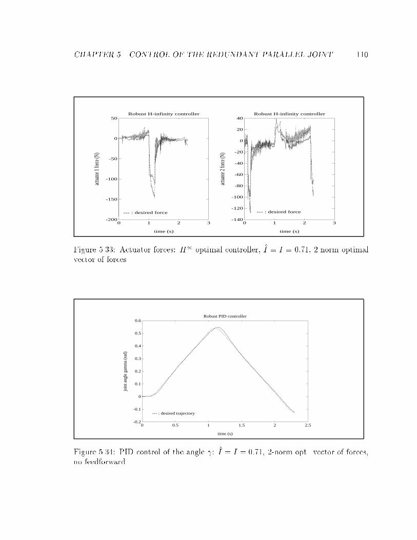
CHAPTER 5. CONTROL OF THE REDUNDANT PARALLEL JOINT 110
-200
-150
-100
-50
0
50
0 1 2 3
time (s)
Robust H-infinity controller
--- : desired force
actua
tor 1
force
(N)
-140
-120
-100
-80
-60
-40
-20
0
20
40
0 1 2 3ac
tuator
2 for
ce (N
)
Robust H-infinity controller
time (s)
--- : desired force
Figure 5.33: Actuator forces: H1-optimal controller, I = I = 0:71, 2-norm optimalvector of forces
-0.2
-0.1
0
0.1
0.2
0.3
0.4
0.5
0.6
0 0.5 1 1.5 2 2.5
Robust PID controller
time (s)
join
t ang
le g
amm
a (r
ad)
--- : desired trajectory
Figure 5.34: PID control of the angle : I = I = 0:71, 2-norm opt. vector of forces,no feedforward

CHAPTER 5. CONTROL OF THE REDUNDANT PARALLEL JOINT 111
-0.2
-0.1
0
0.1
0.2
0.3
0.4
0.5
0.6
0 0.5 1 1.5 2 2.5
Robust H-infinity controller
time (s)
join
t ang
le g
amm
a (r
ad)
--- : desired trajectory
Figure 5.35: H1 control of the angle : I = I = 0:71, 2-norm opt. vector of forces,no feedforward
crossover frequency is lower, which decreases the phase margin and could eventually
destabilize the system. We can observe this phenomenon in Figure 5.36, where the
estimated value of the inertia I = 0:71 is set to I = 0:2. No feedforward is used and
the 2-norm optimal vector of forces is chosen.
The next two experiments are designed to evaluate and compare the robustness of
the PID and the H1-optimal controllers for an overestimated inertia, that is I = 0:36
while I = 0:71. The trajectories are plotted in Figures 5.37 and 5.38. TheH1-optimal
controller clearly oers more robustness and better tracking performance under these
conditions.
In Section 5.3, a variable-bandwidth, nonlinear controller exploiting the hydraulic
damping nonlinear characteristic of the actuator was developed, and a set of step
response experiments are performed to test its eectiveness. The desired step d is
at the middle of the workspace and goes from 0.2 rad to 0.4 rad at t = 1 s. We rst
test the nonlinear controller combined to the PID, and the step responses with and
without the nonlinear controller are shown in Figure 5.39. It should be noted that

CHAPTER 5. CONTROL OF THE REDUNDANT PARALLEL JOINT 112
-0.2
-0.1
0
0.1
0.2
0.3
0.4
0.5
0.6
0.7
0 0.5 1 1.5 2 2.5
Robust PID controller
time (s)
join
t ang
le g
amm
a (r
ad)
--- : desired trajectory
Figure 5.36: PID control of the angle : I = 0:2, I = 0:71, 2-norm opt. vector offorces, no feedforward
-0.2
-0.1
0
0.1
0.2
0.3
0.4
0.5
0.6
0 0.5 1 1.5 2 2.5
time (s)
Robust PID controller
join
t ang
le g
amm
a (r
ad)
--- : desired trajectory
Figure 5.37: PID control of the angle : I = 0:71, I = 0:36, 2-norm opt. vector offorces

CHAPTER 5. CONTROL OF THE REDUNDANT PARALLEL JOINT 113
-0.2
-0.1
0
0.1
0.2
0.3
0.4
0.5
0.6
0 0.5 1 1.5 2 2.5
Robust H-infinity controller
time (s)
join
t ang
le g
amm
a (r
ad)
--- : desired trajectory
Figure 5.38: H1 control of the angle : I = 0:71, I = 0:36, 2-norm opt. vector offorces
there is no feedforward of the desired angular velocity _ d (an impulse). The control
forces for the nonlinear controller combined to the PID and for the PID only are
plotted in Figures 5.40 and 5.41.
Looking at Figure 5.39, it is seen that the step response obtained with the nonlin-
ear controller rises slightly faster than the one obtained with the linear PID controller,
however the settling time of the former appears to be longer. It can also be observed
that the high forces produced by the nonlinear controller tend to create high stress on
the mechanism which results in undesirable discontinuities in the angle measurement.
Figure 5.40 clearly shows that the forces are always less than -200 N and that the
force tracking is quite good when the joint moves in the middle of its workspace.
The nonlinear controller is now combined to the H1-optimal controller and the
procedure is repeated. The step responses are plotted in Figure 5.42 and the control
forces are shown in Figures 5.43 and 5.44. Here it is not clear whether the rise
time is actually less for the nonlinear controller considering the distortion in the

CHAPTER 5. CONTROL OF THE REDUNDANT PARALLEL JOINT 114
0.15
0.2
0.25
0.3
0.35
0.4
0.45
0 0.5 1 1.5 2 2.5
PID + Nonlinear Controller
time (s)
join
t ang
le g
amm
a (r
ad)
... : desired trajectory
--- : PID controller only
Figure 5.39: Nonlinear Controller + PID: I = I = 0:71, Fa = 200 N, 2-norm opt.vector of forces
-600
-500
-400
-300
-200
-100
0
100
0 1 2 3
PID + Nonlinear Controller
time (s)
actua
tor 1
force
(N)
--- : desired force
-600
-500
-400
-300
-200
-100
0
0 1 2 3
actua
tor 2
force
(N)
PID + Nonlinear Controller
time (s)
--- : desired force
Figure 5.40: Actuator forces: nonlinear controller + PID, I = I = 0:71, Fa = 200 N,2-norm optimal vector of forces

CHAPTER 5. CONTROL OF THE REDUNDANT PARALLEL JOINT 115
-150
-100
-50
0
50
100
150
200
250
0 1 2 3
PID controller
time (s)
actua
tor 1
force
(N)
--- : desired force-500
-400
-300
-200
-100
0
100
0 1 2 3
actua
tor 2
force
(N)
PID controller
time (s)
--- : desired force
Figure 5.41: Actuator forces: PID controller only, I = I = 0:71, 2-norm optimalvector of forces
angle measurement. But again, the settling time is considerably shorter for the H1-
optimal controller alone and the step response it produces is better. In both cases the
computed control forces reach high magnitudes well beyond the saturation forces of
the actuators, but that is to be expected since the lead controller is essentially a digital
bandlimited dierentiator which acts on the error between d and . Consequently,
this error being discontinuous at t = 1 s, the computed control torque contains a
pulse that must be produced by the control forces.
Although it is demonstrated that the variable-bandwidth, nonlinear controller
could produce slightly shorter rise times in step responses, the benets obtained
are outweighted by the problems occuring because of the high forces applied on the
mechanism. A stronger, more rigid prototype of the mechanism for which higher
values of the lower bound on the force magnitudes Fa could be used would have to
be built in order to test further the properties of this controller.

CHAPTER 5. CONTROL OF THE REDUNDANT PARALLEL JOINT 116
0.15
0.2
0.25
0.3
0.35
0.4
0.45
0 0.5 1 1.5 2 2.5
H-infinity + Nonlinear Controller
time (s)
joint
angle
gamm
a (rad
)
... : desired trajectory
--- : H-infinity only
Figure 5.42: Nonlinear Controller + H1: I = I = 0:71, Fa = 200 N, 2-norm opt.vector of forces
-600
-500
-400
-300
-200
-100
0
100
0 1 2 3
H-infinity + Nonlinear Controller
time (s)
actua
tor 1
force
(N)
--- : desired force
-3000
-2500
-2000
-1500
-1000
-500
0
0 1 2 3
actua
tor 2
force
(N)
H-infinity + Nonlinear Controller
time (s)
--- : desired force
Figure 5.43: Actuator forces: nonlinear controller + H1, I = I = 0:71, Fa = 200 N,2-norm optimal vector of forces

CHAPTER 5. CONTROL OF THE REDUNDANT PARALLEL JOINT 117
-200
0
200
400
600
800
1000
1200
0 1 2 3
H-infinity Controller
time (s)
actua
tor 1
force
(N)
--- : desired force-2500
-2000
-1500
-1000
-500
0
500
0 1 2 3
actua
tor 2
force
(N)
H-infinity Controller
time (s)
--- : desired force
Figure 5.44: Actuator forces: H1-optimal controller only, I = I = 0:71, 2-normoptimal vector of forces
5.5.2 Impedance and Force Control Experiments
Unstable interactions between a robot and its environment have been a major source
of concern for many researchers in robotics. One way to deal with this class of
problems is to actively control the impedance of the manipulator [Whitney, 1977].
The impedance oered by the PD and the H1-optimal controllers was analyzed in
Section 5.4, and two experiments were designed to verify the theoretical results. The
two experiments are essentially the same as the position control experiments except
that they involve a desired trajectory which goes past a rigid object introduced in
the workspace. No special contact detection algorithm is implemented, thus, after
contact, the actuators just apply increasingly higher forces as the trajectory error
rises. The point of contact is at the end of the rod, about 0.49 m away from the joint
axis. The trajectory is plotted in Figure 5.45 for the PD control system. It can be
noticed that the environment (a long beam made of aluminum) bends signicantly
after contact is made. Nevertheless, no bouncing is apparent on this gure which is

CHAPTER 5. CONTROL OF THE REDUNDANT PARALLEL JOINT 118
quite satisfying. The forces are shown in Figure 5.46 and we can see that actuator 2
saturates.
-0.4
-0.35
-0.3
-0.25
-0.2
-0.15
-0.1
-0.05
0
0.05
0.1
0 0.5 1 1.5 2 2.5
PD Controller
time (s)
joint
angle
gamm
a (rad
)
--- : desired trajectory
Figure 5.45: Contact experiment, PD controller: I = I = 0:71, 2-norm optimal vectorof forces
Figure 5.47 shows the trajectory when the H1-optimal controller is used in the
contact experiment. Again there is no apparent bouncing at the instant where con-
tact occurs, and the environment bends less than it did in the previous experiments
because the open-loop gain of the H1 control system is lower than that of the PD
control system. The control forces produced by the H1-optimal controller are shown
in Figure 5.48, and we can see that they are about ve times smaller than the control
forces produced by the PD controller.
After contact with the environment has been made and detected, it is usually
desirable to regulate the force the robot applies or to make its end-eector track
desired force trajectories. The next experimental results are obtained from basically
the same experiment as before, except that after contact the position controller is
disabled and the force applied on the environment by the end of the rod attached to

CHAPTER 5. CONTROL OF THE REDUNDANT PARALLEL JOINT 119
-50
0
50
100
150
200
250
300
350
400
450
0 1 2 3
PD Controller
time (s)
actua
tor 1
force
(N)
--- : desired force-200
0
200
400
600
800
1000
1200
1400
1600
1800
0 1 2 3
actua
tor 2
force
(N)
PD Controller
time (s)
--- : desired force
Figure 5.46: Actuator forces: contact experiment with PD controller, I = I = 0:71,2-norm optimal vector of forces
-0.4
-0.35
-0.3
-0.25
-0.2
-0.15
-0.1
-0.05
0
0.05
0.1
0 0.5 1 1.5 2 2.5
H-infinity Controller
time (s)
joint
angle
gamm
a (rad
)
--- : desired trajectory
Figure 5.47: Contact experiment, H1-optimal controller: I = I = 0:71, 2-normoptimal vector of forces

CHAPTER 5. CONTROL OF THE REDUNDANT PARALLEL JOINT 120
-20
-10
0
10
20
30
40
50
60
70
0 1 2 3
H-infinity Controller
time (s)
actua
tor 1
force
(N)
--- : desired force-50
0
50
100
150
200
250
300
0 1 2 3ac
tuator
2 fo
rce (N
)
H-infinity Controller
time (s)
--- : desired force
Figure 5.48: Actuator forces: contact experiment with H1-optimal controller, I =I = 0:71, 2-norm optimal vector of forces
the joint (see picture in Figure 3.2) is regulated by the analog lead-lag force controllers.
Contact detection is implemented as a simple check on the dierence between two
samples of the force applied by actuator 2. When this dierence exceeds a threshold
of 10 N, the digital position controller is disabled and the minimun 2-norm vector
of forces corresponding to a torque of -4.91 Nm is used as input to the analog force
controllers, such that the force applied on the environment is approximately 10 N. This
detection scheme is not meant to be general but works well in this case. The rst plot
(Figure 5.49) shows the force applied on the aluminum beam based on measurements
of forces applied by the actuators. Of course these measurements do not indicate
what is really happening at the interface between the beam and the robot's endpoint
because the mechanism is not perfectly rigid. Hence, a ner regulation requires that
a force sensor be mounted at the endpoint.

CHAPTER 5. CONTROL OF THE REDUNDANT PARALLEL JOINT 121
-5
0
5
10
15
20
0 0.5 1 1.5 2 2.5
H-infinity Controller
time (s)
force
(N)
--- : desired force on environment
Figure 5.49: Regulation of force applied on the environment with H1-optimal con-troller, 2-norm optimal vector of forces
The nonlinear controller is also tried in combination with the H1-optimal con-
troller to see if a faster regulation occurs, but this is not the case. The force applied
on the beam is plotted in Figure 5.50.

CHAPTER 5. CONTROL OF THE REDUNDANT PARALLEL JOINT 122
-5
0
5
10
15
20
25
30
0 0.5 1 1.5 2 2.5
H-infinity + Nonlinear Controller
time (s)
force
(N)
--- : desired force on environment
Figure 5.50: Regulation of force applied on the environment with H1-optimal andnonlinear controller, 2-norm optimal vector of forces

Chapter 6
Conclusion
In Chapter 2, a brief comparative analysis of two dierent actuator technologies for
high performance robotics was presented. Electric motors were compared to hydraulic
actuators in terms of their merits on important characteristics such as torque to mass
ratio, torque bandwidth and linearity. Hydraulic actuators with fast suspension-type
valves were found to be superior mainly because of their high torque to mass ratios,
but also because of their extended force bandwidth. Moreover, their force or torque
characteristic can be linearized by feedback.
A high performance hydraulic actuator commercialized by asi was then analyzed
and its highly nonlinear dynamics were modeled. A software simulator implementing
the model in a force control loop demonstrated its usefulness to predict the force
response of the actual system. A simple analog lead-lag force controller was shown
to yield good force bandwidth (100 Hz) and good tracking accuracy.
In Chapter 3, a robotic revolute joint mechanism actuated in-parallel by two
antagonistic hydraulic actuators was designed, built and tested. This mechanism
was shown to oer many advantages over a non-redundant design, such as a large
workspace free of singularities, well-conditioned torque and angle sensing, and the
123

CHAPTER 6. CONCLUSION 124
possibility of controlling internal forces. Although the parallel joint is not truly direct-
drive since the forces are transmitted through a moment arm, it compares nonetheless
favorably to any direct-drive electric motor currently available. For example, its
torque to mass ratio is almost ten times larger than it is for most DC motors.
The kinematics of the parallel joint were derived and an autonomous kinematic
calibration scheme that requires no external measurement of the joint angle was
developed and tested. The kinematic parameters of the prototype were successfully
identied even though the measurement matrix was signicantly noisy. This was
achieved by constraining the nonlinear search to a smaller region in parameter space
by xing (i.e. measuring) two length parameters.
The mapping from actuator forces to joint torque is onto, and hence, an innity
of solutions for the vector of actuator forces exist for a given output torque. This
allowed the calculation of two dierent optimal solutions in the form of minimum-
norm vectors of forces in Chapter 4. The rst minimum-norm vector was a least-
squares solution minimizing the internal force in the joint. The second minimum-norm
vector minimized the maximummagnitude of the actuator forces. It was characterized
and calculated using the theory of dual Banach spaces. Both optimal solutions were
shown to have simple expressions suitable for real-time control. In Chapter 5, it was
demonstrated that these optimal force commands could be easily calculated in less
than 1 ms on a sky Challenger C30 TM computer.
Finally, three position controllers were designed in Chapter 5, of which one was
a simple PD controller while the other two were robust controllers|one based on
the Internal Model Principle and the other based on single-input single-output H1
sensitivity minimization theory. Although the design based on the Internal Model
Principle was carried out in state space, the result was shown to be a simple PID con-
troller for a constant uncertainty model. This controller is robust to slight variations
in the state space model but this has no physical meaning in terms of input-output

CHAPTER 6. CONCLUSION 125
behavior. Hence, the H1 optimal controller appears to be better from the robustness
standpoint because it is robust to variations in the input-output map, i.e. the transfer
function. This explains partly why H1 theory is so popular at the moment.
A series of position control experiments were conducted to assess performance of
the three controllers. The PD controller displayed the best tracking performance,
mainly because the resulting closed-loop system had a larger bandwidth (4 Hz) than
with the other two robust controllers (2.5 Hz). The PID controller showed reasonable
tracking performance, but it was not as robust as the H1 lead controller when bad
estimates of the inertia were used. The angle response of the H1-optimal control
system followed the desired trajectory satisfyingly. Feedforward of the desired angu-
lar acceleration was shown to help greatly trajectory tracking independently of the
structure of the controller, even though the linear trajectory with parabolic blends
displayed discontinuities in its angular acceleration.
A nonlinear controller was designed to modulate the system's bandwidth by im-
posing a lower limit on the valve position magnitudes. This has the eect of shifting
the nonlinear damping characteristic to the right, and hence, it reduces the hydraulic
reaction force for a given piston velocity. Antagonistic actuation allowed the imple-
mentation of this idea on the joint since the vector of actuator forces computed by
the nonlinear controller lies in the nullspace of the transposed jacobian. Only slightly
faster rise times were recorded in the angle step responses with this nonlinear con-
troller, but some problems occured due to the high forces applied by the actuators.
These problems outweighted the small increase in bandwidth obtained.
When a robot makes contact with a sti environment, its impedance determines
how the end-eector will react to the sudden impact. Thus the impedance of the
three joint position control systems were calculated in Chapter 5. The PD controller
and the lead controller yielded impedances similar to that of a nicely damped mass-
spring-damper system, which is what we want. On the other hand, the impedance

CHAPTER 6. CONCLUSION 126
obtained from the PID controller was shown to be undesirably sti at low frequency
because of the integral term|a well-known fact.
Contact experiments were designed and conducted to see if the system would re-
main stable at all, and satisfying angle responses were observed, showing no apparent
bouncing of the end-eector on the hard surface. Force control was also implemented
by detecting the collision and specifying a desired constant torque command, which
was then translated to actuator force commands to the analog force controllers. These
experiments also proved to be successful as the force applied at the endpoint would
rapidly settle to the desired value without showing excessive oscillations.
6.1 Suggestions for Further Research
6.1.1 Modeling of the ASI Hydraulic Actuator
Further investigation into the identication of the linear dynamics of the actuator is
required to ascertain whether the non-minimumphase zeros in the model are artefacts
of the system identication technique, or whether they can be related to specic
distributed-parameter components of the overall system. Since non-minimum phase
zeros place absolute limits on the achievable sensitivity minimization using feedback
control, establishing the physical meaning of these zeros would be of relevance in
further rening the actuator design to achieve even higher performance.
Better experiments will have to be designed for more satisfying models of the
hydraulic damping and friction characteristics. The hydraulic actuator model could
be used to assess the attainable range of mechanical impedance. It would also be
desirable to see the eect of reducing the model order by neglecting some of the uid
high frequency dynamics. The system's ability to act as a force servo or regulator
while the piston is moving will also have to be better assessed and improved.

CHAPTER 6. CONCLUSION 127
Given the fact that the model developed in this research for the asi hydraulic ac-
tuator seems reasonably faithful, it would be interesting to build more sophisticated
linear or possibly nonlinear digital force controllers for it. For example, a nonlinear
observer-based controller could be developed for the model and tested on the real
actuator in order to see to what extent the model can be used as an observer of
the system states, and to nd out if the performance attained would surpass that
obtained by using a simple analog lead-lag compensator. Of course, such a controller
would require a very fast computer and therefore might not be practical. Yet, prelim-
inary experiments have shown that two single-input single-output digital lead force
controllers could be implemented easily on a sky Challenger C30TM computer at a
sampling frequency of 1000 Hz.
The simple linear lead-lag controller used in this research did not show good
robustness properties as it would sometimes make the system break into a limit
cycle for a short time without apparent reason. Hence a more robust force control
law should be developed before a higher level control scheme can be condently
implemented on a multi-actuator mechanism.
6.1.2 Parallel, Redundant Revolute Joint
The mechanism we dealt with in this research has essentially linear dynamics if we
neglect the actuators, but multi-DOF parallel manipulators generally possess highly
nonlinear dynamics. The two linear robust control methods investigated in Chapter 5
could be extended to these mechanisms after implementation of a linearization scheme
performed by feeding back the nonlinear terms of the dynamic equations, as done in
the computed torque method. A convenient characterization of the uncertainty and
disturbance vectors aecting the output of the linearized system should then lead to
an ecient closed-loop control system with nice robustness properties.
A simulator including the nonlinear actuator dynamicmodel could be developed to

CHAPTER 6. CONCLUSION 128
test dierent position and impedance control laws for hydraulically actuated parallel
manipulators.
The autonomous kinematic calibration procedure tested on the parallel revolute
joint could be extended to more complex parallel mechanisms with closed kinematic
chains and partially constrained endpoints. An interesting problem is when there is
no closed-form solution to the direct kinematics of a parallel mechanism: how can one
prove convergence when two iterative schemes are used at the same time to calculate
the endpoint position and to estimate the kinematic parameters?
Finally, new criterions could be used in the force optimization problem, and an-
tagonistic actuation should be investigated further as it has already proven to be a
promising idea in robotics.

Bibliography
[An, Atkeson, Hollerbach, 1988] An, C. H., Atkeson, C. G., Hollerbach, J. M. Model-
Based Control of a Robot Manipulator. Cambridge, Massachusetts: The mit
Press, 1988.
[ASI, 1991] Animate Systems Incorporated (asi) 1991. Advanced Robotic Controller
System Manual. Salt Lake City, Utah.
[Astrom, 1983] Astrom, K. J., Theory and Applications of Adaptive Control|A Sur-
vey. Automatica, Vol. 19, pp. 471486, September 1983.
[Bennett and Hollerbach, 1991] Bennett, D. J., Hollerbach, J. M., Autonomous Cali-
bration of Single-Loop Closed Kinematic Chains Formed by Manipulators with
Passive Endpoint Constraints. ieee Transactions on Robotics and Automation,
Vol. 7, No. 5, October 1991.
[Blackburn, Reethof and Shearer, 1960] Blackburn, J. F., Reethof, G., Shearer, J. L.
(Eds.) 1960. Fluid Power Control. Cambridge: The mit Press.
[Bobrow and Desai, 1990] Bobrow, J. E., Desai, J. 1990. Modeling and Analysis of
a High-Torque, Hydrostatic Actuator for Robotic Applications. Experimental
Robotics I, the First Int. Symp. V. Hayward, O. Khatib (Eds.) Springer-Verlag,
pp. 215228.
129

BIBLIOGRAPHY 130
[Davison and Ferguson, 1981] Davison, E. J., Ferguson, I. J., The Design of Con-
trollers for the Multivariable Robust ServomechanismProblemUsing Parameter
Optimization Methods. ieee Transactions on Automatic Control, Vol. AC-26,
No. 1, February 1981.
[Desa and Roth, 1985] Desa, S., Roth, B., Synthesis of Control Systems for Manipu-
lators Using Multivariable Robust Servomechanism Theory. The International
Journal of Robotics Research, Vol. 4, No. 3, Fall 1985.
[Eppinger and Seering, 1987] Eppinger, S. D., Seering, W. P., Understanding Band-
width Limitations in Robot Force Control. Proc. of the IEEE Conf. on Robotics
and Automation, Vol. 2, 1987.
[Frame, Mohan and Liu, 1982] Frame, J. G., Mohan, N., Liu, T., Hysteresis Model-
ing in an Electromagnetic Transients Program. ieee Trans. on Power Apparatus
and Systems Vol. pas-101, No. 9, September 1982, pp. 34033411.
[Francis and Wonham, 1976] Francis, B. A., Wonham, W. M., The Internal Model
Principle of Control Theory. Automatica, Vol. 12, pp. 457-465, 1976.
[Gille, Decaulne and Pelegrin, 1985] Gille, J. C., Decaulne, P., Pelegrin, M., Dy-
namique de la commande lineaire. Paris: Dunod, 1985. (in french)
[Gottlieb et al., 1990] Gottlieb, G. L., Corcos, D. M., Agarwal, G. C., Latash, M.
L., Principles Underlying Single-Joint Movement Strategies. Multiple Muscle
Systems, Biomechanics and Movement Organization J. M. Winters and S. L.-
Y. Woo (Eds.), New-York: Springer-Verlag, 1990.
[Hayward, 1988] Hayward, V. An Analysis of Redundant Manipulators from Several
View-points. nato Advanced Research Workshop, Robots with Redundancy:
Design, Sensing and Control, A. K. Bejczy (Ed.), Springer-Verlag, 1988.

BIBLIOGRAPHY 131
[Hayward, 1991] Hayward, V. Borrowing Some Design Ideas From Biological Manip-
ulators to Design an Articial One. Robots and Biological Systems, NATO Ad-
vanced Research Workshop. Dario P., Sandini, G., Aebisher, P. (Eds.), Springer-
Verlag, 1991.
[Hollerbach, Hunter and Ballantyne, 1991] Hollerbach, J. M., Hunter, I. W., Bal-
lantyne, J., A Comparative Analysis of Actuator Technologies for Robotics.
Robotics Review 2, O. Khatib, J. Craig, T. Lozano-Perez (Eds.), Cambridge:
MIT Press, Massachusetts, 1991.
[Hunt, 1983] Hunt, K. H., Structural Kinematics of In-Parallel-Actuated Robot
Arms, Trans. ASME, J. Mech., Transmission, Automat. Design., Vol 105, pp.
705712. 1983.
[Jacobsen et al., 1991] Jacobsen, S. C., Smith, F. M., Backman, D. K., Iversen, E.
K., High Performance, High Dexterity, Force Re ective Teleoperator II. ANS
Topical Meeting on Robotics and Remote Systems, Albuquerque, NM, Feb. 24
27, 1991.
[Kerr and Roth, 1986] Kerr, J., Roth, B., Analysis of Multingered Hands The In-
ternational Journal of Robotics Research, Vol. 4, No. 4, Winter 1986.
[Khatib, 1987] Khatib, O. A Unied Approach for Motion and Force Control of Robot
Manipulators: The Operational Space Formulation. ieee Journal of Robotics
and Automation, Vol. RA-3, No. 1, February 1987.
[Kuo and Wang, 1991] Kuo, C.-Y., Wang, S.-P. T., Robust Position Control of
Robotic Manipulator in Cartesian Coordinates. ieee Transactions on Robotics
and Automation, Vol. 7, No. 5, October 1991.

BIBLIOGRAPHY 132
[Kurtz, 1990] Kurtz, R. L. Kinematic and Optimization of a Parallel Robotic Wrist
MechanismWith Redundancy.McGill Research Center for Intelligent Machines
Technical Report TR-CIM-90-2, January 1990.
[Luenberger, 1969] Luenberger, D. G., Optimization by Vector Space Methods. New-
York: John Wiley & Sons, 1969.
[Luh, Walker and Paul, 1980] Luh, J. Y. S., Walker, M. W., Paul, R. P. C., Resolved-
Acceleration Control of Mechanical Manipulators. ieee Trans. on Automatic
Control, Vol. AC-25, No. 3, June 1980.
[McLain et al., 1989] McLain, T. W., Iversen, E. K., Davis, C. C., Jacobsen, S. C.,
Development, Simulation, and Validation of a Highly Nonlinear Hydraulic Ser-
vosystem Model. Proc. of the 1989 American Control Conference, aacc. Pis-
cataway: ieee, 1989.
[Nahon, 1990] Nahon, M., Optimization of Force Distribution in Redundantly-
Actuated Robotic Systems. Ph.D. Thesis, Department of Mechanical Engineer-
ing, McGill University, 1990.
[Paul, 1972] Paul, R. C., Modeling Trajectory Calculation and Servoing of a Com-
puter Controlled Arm. Stanford Articial Intelligence Laboratory A.I. Memo
177, Stanford University, Stanford, CA, September 1972.
[Shearer, 1983] Shearer, J. L., Digital Simulation of a Coulomb-Damped Hydraulic
Servosystem. Trans. asme, J. Dyn. Sys., Meas., Contr. Vol. 105, December
1983, pp. 215221.
[The Math Works Inc., 1990] The Math Works Inc. 1990. simulab: A Program for
Simulating Dynamic Systems. (user's guide)

BIBLIOGRAPHY 133
[Slotine, 1985] Slotine, J.-J. E., The Robust Control of Robot Manipulators. The
International Journal of Robotics Research, Vol. 4, No. 2, Summer 1985.
[Spong and Vidyasagar, 1987] Spong, M. W., Vidyasagar, M., Robust Linear Com-
pensator Design for Nonlinear Robotic Control. ieee Journal of Robotics and
Automation, Vol. RA-3, No. 4, August 1987.
[Spong and Vidyasagar, 1989] Spong, M. W., Vidyasagar, M., Robot Dynamics and
Control. New-York: John-Wiley & Sons, 1989.
[Threlfall, 1978] Threlfall, D. C., The Inclusion of Coulomb Friction in Mechanisms
Programs with Particular Reference to dram. Mech. and Mach. Theory Vol.
13, 1978, pp. 475483.
[Vidyasagar, Bertschmann and Sallaberger, 1988] Vidyasagar, M., Bertschmann, R.
K., Sallaberger, C. S., Some Simplications of the Graphical Nyquist Criterion.
ieee Transactions on Automatic Control, Vol. AC-33, pp. 301305, 1988.
[Vischer and Khatib, 1990] Vischer, D., Khatib, O., Design and Development of
Torque-Controlled Joints. Experimental Robotics I, the First Int. Symp. V. Hay-
ward, O. Khatib (Eds.), pp. 271286, Springer-Verlag, 1990.
[Walters, 1967] Walters, R., Hydraulic and Electro-Hydraulic Servo Systems. Cleve-
land: crc Press, 1967.
[Whitney, 1977] Whitney, D. E., Force Feedback Control of Manipulator FineMotion.
ASME Journal of Dyn. Systems, Measurement, and Control, June 1977, pp. 91-
97.
[Whitney, Lozinski, Rourke, 1986] Whitney, D. E., Lozinski, C. A., Rourke J. M.,
Industrial Robot Forward Calibration Method and Results. asme J. of Dyn.
Syst., Meas., and Cont., Vol. 108, March 1986.

BIBLIOGRAPHY 134
[Winters, 1990] Winters, J. M., Hill-Based Muscle Models: A Systems Engineering
Perspective.Multiple Muscle Systems, Biomechanics and Movement Organiza-
tion, J. M. Winters and S. L.-Y. Woo (Eds.), New-York: Springer-Verlag, 1990.
[Zames, 1981] Zames, G., Feedback and Optimal Sensitivity: Model Reference Trans-
formations, Multiplicative Seminorms, and Approximate Inverses. ieee Trans-
actions on Automatic Control, Vol. AC-26, No. 2, April 1981.
[Zames and Francis, 1983] Zames, G., Francis, B. A., Feedback, Minimax Sensitivity,
and Optimal Robustness. ieee Transactions on Automatic Control, Vol. AC-28,
No. 5, May 1983.
[Francis, Helton and Zames, 1984] Francis, B. A., Helton, J. W., Zames, G., H1-
Optimal Feedback Controllers for Linear Multivariable Systems. ieee Transac-
tions on Automatic Control, Vol. AC-29, No. 10, October 1984.

Appendix A
Partial Derivatives of FB
These expressions can be used only when > 0.
@FB@k1
= 2 cos
1 r2 21
21
! 2 sin
0@ 21r
21 + r2 21
!2
1
1A1=2 1 r2 21
21
!
@FB@k2
= 22 + cos
1(21 + r2 21) + 2r sin
0@1
21 + r2 21
21r
!21A1=2
@FB@r
= 2k2 4r + cos
"(k1 k2)
1 +
r2 2121
!+ 22
1 +
r
1
#
+ 2 sin
264(k2 + 2r)
0@1
21 + r2 21
21r
!21A1=2
2
0@ 21r
21 + r2 21
!2
1
1A1=2 (k1 + 2r)(21 k21)
2r21
!375
135

APPENDIX A. PARTIAL DERIVATIVES OF FB 136
@FB@10
= 221
cos 1 +22 sin 1
1
0@ 21r
21 + r2 21
!2
1
1A1=2
@FB@20
= 22
@FB@
= 21
sin (21 + r2 21) + 22r cos
0@1
21 + r2 21
21r
!21A1=2

Appendix B
Calibration Algorithm
Implemented on MatlabTM
% This command file implements the Levenberg-Marquardt algorithm to
% calibrate the kinematic parameters of the parallel revolute joint given
% a reasonable estimate. The matrix rhomeas must be in the workspace.
% The file kincalibjoint.mex4 calculates the partial derivatives of FB
% and also FB itself.
% The parameters r (parmest(3)) and lambda2 (parmest(2))
% must be measured accurately because they scale the mechanism.
sigma = 1e-8;
alpha = .001; % This constant controls the speed of convergence
% and gets us through the singularities.
epsilon=.0000001;
FBmin = 1;
i=0;
137

APPENDIXB. CALIBRATIONALGORITHM IMPLEMENTEDONMATLABTM138
normFB = 2*sigma;
% Make sure that the results of the squareroot operations in
% kincalibjoint.mex4 are real
if (parmest(1)-parmest(3)) >= (parmest(4)-max(-rhomeas(:,1)))
parmest(1)=parmest(4)-max(-rhomeas(:,1))-epsilon+parmest(3);
end
while ( (normFB > sigma) & (i < 10000) )
% Calculate the jacobian matrix C and FB
for i=1:50
C(i,:)=kincalibjoint(parmest',rhomeas(i,:));
end
% Calculate deltaparm and new estimate
FB=C(:,7);
C=[C(:,1) C(:,4:6)];
D=inv(C'*C+alpha*eye(4));
deltaparm=-D*C'*FB;
parmest=[(parmest(1)+deltaparm(1));parmest(2);parmest(3); ..
(parmest(4:6)+deltaparm(2:4))];
if max(abs(1000*FB)) < alpha
alpha = alpha/1000;
end

APPENDIXB. CALIBRATIONALGORITHM IMPLEMENTEDONMATLABTM139
normFB=max(abs(FB))
if normFB < FBmin
FBmin = normFB;
bestparmest = parmest;
end
% Make sure that the results of the squareroot operations in
% kincalibjoint.mex4 are real
if (parmest(1)-parmest(3)) >= (parmest(4)-max(-rhomeas(:,1)))
parmest(1)=parmest(4)-max(-rhomeas(:,1))-epsilon+parmest(3);
end
clear C
i=i+1;
end
parmest


![3. Nat. OL Kandersteg 2019 56.Thuner-OL - olg-thun.ch · [Hier eingeben] 3. Nat. OL Kandersteg 2019 56.Thuner-OL Sonntag 25. August 2019 Nationaler OL Langdistanz Lauf zur OL-Nachwuchsmeisterschaft](https://img.dokumen.tips/doc/110x75/5d672ac688c99340518b57c4/3-nat-ol-kandersteg-2019-56thuner-ol-olg-thunch-hier-eingeben-3-nat.jpg)


![3. Nat. OL Kandersteg 2019 / 56.Thuner-OL - olg-thun.ch · [Hier eingeben] Die OLG Thun lädt alle OL-Läufer und OL-Läuferinnen herzlich ein zum: 3. Nat. OL Kandersteg 2019](https://img.dokumen.tips/doc/110x75/5e09501c1231581f421642dc/3-nat-ol-kandersteg-2019-56thuner-ol-olg-thunch-hier-eingeben-die-olg.jpg)