Embed Size (px)
Citation preview

Oil Prices, Geography and Endogenous Regionalism:
Too Much Ado About (Almost) Nothing∗
Daniel Mirza†
Habib Zitouna‡
Abstract
This paper studies the effect of oil prices on the geography of international trade. We modeltransport costs as a function of variable and fixed costs. By affecting the first cost component,oil prices can then modify the structure of transportation costs across partners. This, we argue,acts as a factor of distortion in relative prices, thereby creating a reallocation of trade at theexpense of remote countries. In that respect, an increase in oil prices should favor regionalism.This mechanism is empirically tested using data on US bilateral imports and transportationcosts. The empirical results are consistent with the theoretical intuition. But, the elasticity offreight rates to oil prices, directly linked to geographical distance, appears to be low: between0.088 for close to US countries and 0.103 for faraway ones. We then estimate the contributionof the dramatic increase in oil prices, in recent years, to relative changes in the countries’probability to export to the US (extensive margins) along with their relative market shares(intensive margins). We find that the recent oil price increases that took place after 1999 havehad only a maigre contribution: the last oil shock had contributed marginally to increase Canadaand Mexico’s relative performance.
JEL classification: F15, F19, F20, L91Keywords: Regionalism, Oil Prices, Geography, Transport
∗We wish to thank Florent Pigeon and Emmanuel Milet for excellent research assistance as well as MatthieuCrozet for his very helpful comments on an earlier draft of this paper.
†GERCIE-University Francois Rabelais and GERCIE (Tours, France), CEPII (Paris), email:[email protected]
‡High School of Economic and Commercial Sciences of Tunis(ESSECT) Tunisia, email:[email protected]

1 Introduction
In less than a decade, nominal oil prices have been multiplied by 7, raising from about 20US$
per barrel to reach a peak of 146$ during July 2008. Since then, oil market prices have been
experiencing a sharp return. The 2008 financial crises and the expected dramatic effects it
may produce on the real economy, reversed the expectations on oil capacity supply, ending by
the same token the speculation on oil prices. Many observers note, however, that the drop is
temporary. After recovery, it is probable that oil resources will experience a shortage, shifting
prices upward again.1
What are the implications for globalization of changes in oil prices? Some observers already
note that one effect of oil shocks is to reverse globalization by reallocating flows in favor of more
regionalism. 2 Although the idea is appealing it has never been tested. In the trade literature,
three analytical papers we are aware of link oil prices to trade. The first is that of Backus and
Crucini (2000) who look at the impact of oil shocks on the trade balance through changes in
the terms of trade. On the link going through transportation costs, two other papers discuss
the impact by considering implicitly or explicitly, that oil price shocks can act as a global tax,
affecting freights and trade flows at the same pace. Hummels (2007) shows regression results of
freight costs where an oil price explanatory variable is independently included. It appears with
a positive and statistically significant coefficient. More recently, Bridgman (2008) simulates a
Ricardian model of trade where energy is used as an input in the shipping technology of trading
the industrial good. In the simulated model, he shows that transportation costs slow the growth
1Hamilton’s (2008) work is consistent with such a prediction. He tends to show very clearly that the scarcityof oil resources has been more relevant to explain recent years price increases than ever before.
2Rubin and Tal (2008) is one policy brief article we know about that considers the impact of oil prices onglobalization. But the authors work remain too much descriptive to be able to draw out some solid conclusionson the nature and the extent of the link between oil prices, transportation and global/regional trade.
1

of international trade: during the seventies and beginning of the eighties oil shocks period, the
simulated effect even offset that of the decline in tariffs.
This paper considers a different view. We examine the hypothesis that oil prices affect
differently transportation costs across partners, leading to more regionalism. By distorting
relative prices of goods, an increase in oil values provokes a reallocation of resources across
countries and thus have implications for national and global welfare. More intuitively, if one
believes that an increase in oil prices makes more distant partners less competitive, then one
would expect oil prices to favor regionalism, thus acting as a resistance force against long distance
trade. Oil price increases might then act on welfare as regional trade agreements (RTAs) would
do. They would divert trade flows from more efficient (or low cost) partners to less efficient
partners, resulting in a welfare loss for the importing country. For close exporters however,
oil price increases would then be welfare creating. Nevertheless, there are two main differences
between oil effects and RTAs effects. First, oil shocks would favor regionalism in an endogenous
manner through market forces, while RTAs are government type interventions. The second
difference is a corollary of the first one: oil price increases act as a tax on consumers’ revenue,
although without any compensation via government revenues.
The regionalism effect of oil prices has also implications for health and the environment.
Although greenhouse gas emissions would be lowered globally because of less volumes shipped
over long distances, the relocation of production should increase, in turn, local air pollution.
More rigourously, how can oil prices affect trade costs and thereby the distribution of trade
flows? Under the assumption that transport costs are proportionally linked to oil prices, trade
theory suggests that an increase in the value of oil decreases imports from the rest of the world
but without changing import distribution across partners. That is because a global oil shock
2

should increase all prices proportionally, thus leaving all relative prices in the manufacturing
sector unaffected.
If, however, transport costs do not respond proportionally to oil prices the distribution of
trade costs and trade flows among partners can be altered. In this paper, we consider a general
transport cost function whereby the cost of shipping a good implies variable but also fixed costs
and then take it to the test. This simple although realistic assumption makes the impact of oil
shocks depend on the extent to which transport is governed by variable costs relative to fixed
ones. We then discuss how oil prices in this more general form can be affecting the geography
of trade. It turns out that more distant economies suffer more from an increase in oil prices
than closer trading partners. That is because oil prices affect variable costs, which share in total
costs increases with longer distance.
In a second step, we embody this new technology function of transport into a gravity equation
and discuss how oil prices affect trade flows through changes in transportation charges.
In order to estimate empirically the oil impact on trade geography, we use Robert Feenstra’s
US bilateral imports and freight charges data at the SITC4 product level (over 1000 products).
Alternatively, in order to account for transport modes in our equations, we use the same type
of data by mode of transport kindly provided by David Hummels. The two series are available
for the period 1974-2001. We first find that the elasticity of transport costs to oil prices to
be around 0.1, where an observed country is at a median distance from the US. However, it is
around 0.103 for long distance exporters (more than 10,000 kilometers) and around 0.088 for
closer ones (less than 3,000 kilometers). Oil price changes lower then close countries’ relative
transport costs at the expense of distant partners. This has implications for trade flows. After
estimating an elasticity of export to US market shares to freight rates to be around 1.12, we
3
estimate an elasticity of relative market shares to oil prices to be around 0,013 for close to
the US countries and -0,004 for faraway ones. We then simulate the contribution of last years
dramatic changes in oil prices to market share changes into the US market. We find that the
recent oil shock have had a maigre contribution: it marginally narrowed the observed decrease
in Canada and Mexico’s shares and had a small if not almost insignificant negative contribution
on India and China’s relative growth shares. Besides, we also look at the extensive margins
by trying to estimate and then simulate the impact of the shock on the relative probability to
export. Here too, we find that Canada and Mexico increase their relative propensity to export
following the shock compared to India and China’s likelihood of exports. But these changes are
very small with respect to the huge increase in oil prices observed during the last shock.
The paper is organized as follows: section 2 displays the theoretical framework and develops
the empirical specification. In section 3, the data used is described and some stylized facts are
presented. The econometric results are then presented in section 4. Section 5 estimates the
contribution of oil price increases in recent years to total market share changes. The last section
concludes.
2 The Analytical framework
2.1 The oil-price effect on transport costs
In this section, we propose a theoretical formulation of transport costs in which we highlight
the importance of fixed costs of transport as a source of the non proportional response to oil
prices.
Transport costs in our framework are born out of variable costs, V C, and fixed costs, FC.
Consider first, variable costs. As in Hummels and Skiba (2004), the freight charge per unit
4

transported from i to a given importing country, say the US, involves two types of variable
costs: a price-related component and a non-price related component. Secondly, let us assume
that some fixed costs FC are spent over the year say, for vessel management and maintenance.
The higher the quantities q that are shipped, however, the lower are the fixed costs to bear per
ton of transport. Hence, assume the following additive unit transport cost function (or per ton
cost function):
uci,US = ci,US + pβi +
FC
qi,US(1)
where uci,US is the total cost of transporting one ton of merchandize and ci,US represents
the technology for transporting any given ton of good from i independently of its FOB price
pi. Besides, pβi is a premium charged that is function of the price (with β ≥ 0). In fact, prices
reveal the quality of the goods to be shipped and high quality goods ask for higher insurance
and handling costs in transportation.
Next, let us assume that the non-price related component ci,US is proportional to distance.
Indeed, if the shipping distance doubles one expects to use twice as more oil and, say, labor
hours. Thus, let ci,US = disti,US.f(poil, w) where disti,US represents the distance between i and
the US, and f being a technology function of transport per km, positively related to oil prices
poil and on-board factor prices w. This specification is intuitive: for a zero distance, neither oil
nor on-board labour are used to ship the merchandize.
Thus, oil affects the variable component ci,US through its impact on the technology cost
f(.). Nevertheless, the pass-through to the total cost of transportation uci,US depends on the
extent to which the latter is governed by variable costs relative to fixed costs in the transport
sector. Let sc equals the variable share in total costs of shipping. A simple computation of the
5

elasticity of transportation costs to oil prices gives the following:
ǫuc/poil=
d(uc)/uc
d(poil)/poil= sc.
d(ci,US)/ci,US
d(poil)/poil
= sc.d(f(.))/f(.)
d(poil)/poil
How can geographical distance affect the sensitivity of transport costs to oil prices ? Distance
can make transport costs more sensitive to oil prices through sc. The explanation is simple: an
increase in the shipping distance of a given quantity and at a given price, increases the variable
costs while leaving fixed costs unaffected. As the share of variable costs is higher for distant
partners than for close ones, transportation costs from distant partners become more sensitive
to oil shocks than transportation charge of goods that are shipped from close sources.
For estimation purposes, let us divide equation 1 by the price of the good. We obtain an
expression of freight rates, fr:
fri,US =1
pi
[ci,US + pβ
i +FC
qi,US
](2)
From 2, and expressing the fixed costs component by fci,US = (FC/qi,US) (i.e. fixed costs per
ton of exported good), we can compute the proportional change in freight rates as a function of
changes in variable and fixed rates and changes in the price of the good. Hence, let sfc represent
the share of fixed costs in total costs, and sp represent the share of the good’s price component
of freight costs. We thus obtain:
d(fri,US)
fri,US= sc.
d(ci,US)
ci,US+ (sfc).
d(fci,US)
fci,US+ (β.sp − 1)
d(pi)
pi(3)
6

Equation 3 inspires our econometric specification. It tells that every increase in the variable
costs component (ci) due to oil price increases is passed through freight rates. This pass-through
is higher when the share of this component to total costs is high. Geographical distance, as
mentioned earlier, increases this share. Besides, because of returns to scale born by fixed
costs, an increase in quantities that are shipped reduces the fixed costs of transport thereby
reducing the freight charges. Finally, considering the reasonable assumption that the elasticity
of transport costs to the prices of shipped goods to be lower than unity (0 < β < 1), the
corresponding elasticity of freight rates should be then negative and between 0 and -1. The
lower the parameter β and the share of the price component in total costs of transports are,
however, the higher is the negative relationship between prices and freight rates. In the extreme
case where prices do not affect transport charges per ton, all increases in prices should then
proportionally reduce freight rates (i.e. cost of transport per dollar of the good).
To sum up, freight rates should depend positively on factor costs bared over the whole
distance trip and negatively on the quantities and prices of the goods to be shipped. Thus,
after adding a time subscript t and a product subscript k where suitable and removing the US
subscript to simplify notations, we estimate the following log linear equation:
ln(fri,k) = β1+β2.ln(disti)+β3.ln(poil)t.ln(disti)+β4ln(quantityit,k)+β5ln(UVit,k)+controls+eit,k
(4)
As already mentioned, oil prices affect trade costs through distance: at 0 distance, oil is not
used and oil prices should not enter the equation anymore. Besides, factors other than oil, also
related to distance, are used in the transport technology f (like the number of hours worked by
on-board personnel). As we do not have access to prices of factors other than oil we introduce
7

distance on its own to capture the variation of these other factors3. The quantity variable
representing the quantity that is shipped, should capture economies of scale in the transport
technology while Unit Values (UV ), represent prices of goods and should reduce freight rates
as mentioned above.
Note that we include some control variables: First, we add a contiguity variable (contiguity),
a dummy variable indicating if partners share a common border to take into account the fact
that across border countries might have more developed transportation networks between them,
thus exhibiting further reduction in transport costs. In order to cover better the differences in
transport technologies and their impact on costs, however, we add 3 transport modes dummies
(vessel, land and air). We also add a time trend to our equation and where suitable, account
for some product and/or exporting countries effects.4
For small variation of oil prices, the corresponding elasticity of transport cost is:
dln(frkjt)
dlnpoil= β3.ln(distj)
However, in section 5, we apply our coefficients to estimate the contribution of oil shocks to
regionalizing trade. Oil shocks imply large variations of oil prices, however. As log differences
cannot be interpreted as growth rates in periods of large variations of oil prices, an adjustment
is needed in this case5. The proportional change in freight rates can be then estimated by:
3We do not have access to prices of factors other than oil. One could imagine introducing wages in thetransport sector for each partner country to represent on-board labour costs. This is not, however, a good ideabecause a big proportion of international transportation is served by ships and carriers that do not have the samenationality than the country of exports and/or imports.
4Ideally, we would have liked to include time fixed effets instead of a trend. Unfortunately, the inclusion oftime effects exhibited high multicollinearity with the distance and the interaction term (distance x oil prices)variables, with a variation inflation factor (VIF) largely exceeding acceptable values.
5see proof in appendix A.
8
d(frkjt)
(frkjt)=
(1 +
d(poil)
poil
)β3.ln(dist)
− 1
2.2 The trade equation
We are interested in studying the impact of oil prices on export market shares, through changes
in transport costs. To this end, we need to model a trade equation as a function of transportation
costs, from which we can infer an impact on market shares.
We use a traditional standard monopolistic model of trade. Assume a representative US
consumer with CES preferences over a given differentiated product k produced in different
varieties v. The sub-utility function can be represented by:
Uk,US =
[∑
i
∫
vq(σ−1)/σi,v dv
]σ/(σ−1)
, i = 1..I v = 1..V ∈ k
Where qi,v is consumption of variety v originating from country i.
Assume pi is the FOB exporter’s price of any variety v produced in country i (prices of all vari-
eties equal at equilibrium) and τi,k > 1 is the trade cost (one plus ad-valorem costs) associated
to exporting some variety of a product k to the US.
Maximizing the utility subject to budget constraint yields the following demand function
per variety:
qi,v = qi =
(τi,kpi
PUS,k
)−σ YUS,k
PUS,k(5)
where PUS,k =(∑
i
∫v(pi,vτi,k)
−(σ−1)) −1
σ−1 is the CES price index and YUS,k is the importer’s
expenditure that is spent on all varieties of the product k.
Recall that in the standard model each of the ni,k firms in the market produce and export
9

1 variety of good k from country i to the US market. After introducing a time subscript, total
quantities of good k imported from i at time t is then given by the following expression:
mikt = ni,k,tτiktqit = niktτ−(σ−1)ikt p
(−σ)ikt
YUS,kt
P 1−σUS,kt
(6)
Note that many variables can approximate the trade costs (τikt): along with the transport
costs (frikt), we approach these costs by ad-valorem tariff rates (tariffikt) and a series of
country and year effects. For more tractability, we assume τ to take the following functional
form ln(τikt) = aln(frikt)+bln(tariffikt)+fei +fet where a and b are two positive parameters
while fei and fet are country and year fixed effects. Besides, we can ideally capture theYUS,kt
PUS,kt
term by (product*time) cross effect (fekt). But in most specifications we were constrained by
STATA’s difficulties of processing very big matrix calculations, and thus opted for a simple
product effect fek as an alternative to our cross effect.
Taking the log of each variable, approximating the number of exporting firms by the GDP of
the exporting country (GDPit), the prices by unit values (UVikt), we can estimate the following
basic equation:
ln(mikt) = −a.(σ−1)ln(frikt)−b.(σ−1)ln(tariffikt)+(−σ)ln(UVikt)+λln(GDPit)+fei+fek+fet
(7)
This specification holds as long as freights are exogenous. But, the preceding section shows
that they are not: freight charges depend in turn, on quantities and unit values. Besides, freight
charges and trade flows might be related to some common unobservable factors (think of the
quality of reporting data at the US borders or a macroeconomic shock in some US partner
10

country, hitting its transporters and producers alike). We handle these difficulties by running
3SLS regressions where both equations 7 and 4 are run simultaneously and where the residuals
of both equations are taken to be also correlated to each other.
However, our main purpose here is to link the variability of oil prices to changes in market
shares, not changes in absolute values of trade flows. In other words, we do not want to look at
how Canadian or Mexican exports to the US are being affected in absolute values by oil shocks.
Instead, we are more interested here in how Canadian and Mexican trade shares compared to
those of other exporting countries to the US are being affected after a jump in oil prices. In
what follows, we define a strategy that allows to do this work by estimating a relative (rather
than absolute) equation of trade.
Let us transform first, each of the variables into (geometric) means. The last equation
becomes:
m.,k = n.,kτ−(σ−1).,k p
(1−σ).,k
(YUS,k
P 1−σUS,k
)(8)
where for each variable y: y.,k =∏
i y1/Ii,k presents the geometric mean over all exporting
countries to the US.
Then, divide (6) by (8) in order to obtain a relative market shares equation:
Rmi,k = Rni,k Rτ−(σ−1)i,k Rp
(−σ)i,k (9)
where for each variable y, Ryik =yi,k
y.k. Notice from above that the term
YUS,k
PUS,kdisappears
when expressed in terms of the average exporter.6.
6As all exporters face the same demand (from US) and the same market price index, YUS,k and PUS,k willthen equal respectively YUS,k and PUS,k
11

Again, we approximate each of the theory variables by their observable counterparts (prices
by unit values, trade costs by freights, tariffs and country fixed effects, etc...) express them in
relative terms, add a time index, to obtain the following alternative specification to run:
ln(Rmikt) = −a(σ − 1)ln(Rfrikt)− b(σ − 1)ln(Rtariffikt)− σln(Rpikt) + λln(RGDPit) + Rfei
(10)
Hence, whether we run the gravity specification in absolute values (7) or in relative values
(10), the theory suggests that the coefficients one should obtain have to be comparable. From
there, one can either compute changes in relative trade shares by using the coefficients obtained
from running equation (7) or by using the coefficients obtained from running equation (10).
Nevertheless, in the last equation too, one still has to account for the endogeneity of trans-
portation costs. We had actually tried to run again a 3SLS where both equations of trade and
transport cost were being expressed in relative terms. But it turned out that in the transport
equation, changes in the interaction variable (Oil prices*distance) and changes in distance, when
they were both expressed in relative terms, were highly collinear7. Instead, we account for endo-
geneity here by using an instrumental variable specification where freights are instrumented by
variables which are supposed to shift the freight equation while being orthogonal to the residual
of the trade share equation. For instance, the modes of transport variables are good candidates
since they affect freights via the supply side of the international transport market and without
shifting a priori the trade shares’ curve (and a fortiori its residual). More on this issue in the
econometric section.
7The VIF computed in STATA reached around 100.
12

Recall by now that the objective of our paper is to estimate the impact of oil prices on
relative market shares through their induced effect on freight rates. The oil-price effect on
relative imports will be then estimated in reference to the following formulae:
dln(R.mikt)
d(poil)t=
dln(R.mikt)
dln(R.frikt).dln(R.frikt)
dln(poil)t= − a(σ − 1)β3.ln(R.disti)
In large variation periods, however (see annex) we can estimate the effect by:
dR.mikt
R.mikt= − a(σ − 1)
[(1 +
dpoil
poil
)β3.ln(R.disti)
− 1
](11)
3 Data and Stylized Facts
For our stylized facts as well as the econometric study, we use Robert Feenstra’s NBER US
bilateral imports dataset. Bilateral imports are reported - in FOB values and physical quantities
(tons)- along with freight charges data at the SITC 4-digits product level (over 1000 products).8
The data is available from 1974 to 2001. We drop all the observations for which quantities cannot
be converted to tons. Besides, we are mainly interested in oil as an input in the international
transport sector, not as an output to be traded. Hence, we exclude from the empirical analysis
all oil-type products (sitc2 sectors 33 and 34).
Feenstra’s dataset does not distinguish between modes of transportation, generally made by
Air, Sea and/or Land. It lists flows of goods and transport aggregated over all of these modes.
Each mode implies a different technology of transport, however. In order to control for this
in our empirical freight equation, we complete Feenstra’s data by adding a mode of transport
8Data is made available on the NBER website: http://www.nber.org/data/. It is described in Feenstra et al.(2001).
13

information provided by the US Bureau of Transportation Statistics and readily made available
by David Hummels. These data distinguish between Air and Sea transportation to the US and
is observed from each exporting country and for each SITC 4-digits level product reported over
the considered period.9 Finally, by merging both datasets and comparing figures, we could easily
guess the products that were also shipped by Land. So, we will add, in our regressions three
dummy variables (land, vessel and air) taking on 1 whenever positive flows for each transport
mode are observed and 0 otherwise10.
Finally, we use the CEPII’s database on distances freely available online.11 As for macro
variables, such as GDP, we use the World Development Indicators published by the worldbank.
Figure 1: Relative average freight rates & oil prices
0.5
11.5
2
10 15 20 25 30 35
a/ Close = distance <5000 Km and Remote = distance >5000 Km
b/ Weighted average fret rates (per Ton/km) computed over all partners to US
oil price
We
igh
ted
av
era
ge
fre
t ra
tes
for
clo
se c
ou
ntr
ies
We
igh
ted
av
era
ge
fre
t ra
tes
for
rem
ote
co
un
trie
s
9The data is readily available from http://www.mgmt.purdue.edu/faculty/hummels10By cross-checking Feenstra’s data with that of Hummels we noticed that from 1982 to 1988, the aggregated
data for Mexico and Canada reported in Feenstra did not include land transport for these years. This is anotherreason why it has been important to include transport-mode dummy variables in our transport costs regressions.We have removed, however, these problematic observations from the stylised facts below.
11http://www.cepii.fr/francgraph/bdd/distances.htm
14

Figure 2: relative average transport costs per Ton & oil prices
0.5
11.5
10 15 20 25 30 35
oil price
a/ Close = distance <5000 Km and Remote = distance >5000 Km
b/ Weighted average transport costs (per Ton/km) computed over all partners to US
We
igh
ted
av
era
ge
tra
nsp
ort
co
sts
for
clo
se c
ou
ntr
ies
We
igh
ted
av
era
ge
tra
nsp
ort
co
sts
for
rem
ote
co
un
trie
s
Figure 3: Market shares & oil prices
.2.4
.6.8
10 15 20 25 30 35oil price
Close = distance <5000 Km and Far = distance >5000 Km
Distance to US Close Far
Ma
rke
t sh
are
15

Before turning to the econometric study, we display some stylized facts. Our main argument
is that transport costs and market shares should not respond proportionally to oil-prices varia-
tions across exporting countries to the US. More specifically, higher oil prices should favor more
close countries by reducing their relative costs and increasing their market shares with respect
to remote ones.
We thus split the countries into two groups: One far from the US group and another close to
the US group and compute their relative average transport costs and market shares.
The close countries’ (resp. far) group comprises all countries which are at a distance that is
less (resp. more) than 5000 km from the US. Then, we compute for each year average transport
costs of close countries in terms of faraway countries12. We expect relative transportation costs
of close countries to decline with oil prices. Figure 1 confirms the negative relationship between
relative freight rates of close countries and oil-prices. In order to check for robustness, figure
2, offers the same picture by replacing freight rates by a measure of transportation charges per
ton13.
In figure 3, using the same data, we illustrate the relationship between market-shares and
oil-prices. Again, countries are divided into the same two groups than previously. Figure 3
provides a message consistent with that revealed by the prior figures: an increase in oil-prices
seems to be associated with increases in the market share of close countries at the expense of
faraway countries.
12Note that transport costs and freight rates are observed at the year, product and export country levels. Inorder to obtain a time varying representative indicator of transport costs over the whole samples of close andfaraway countries, we double average over the product and partner dimensions.
13In fact, a third graph not reported here shows that transportation charges per Ton, when plotted indepen-dently for close and faraway countries, both move upward when the oil price increases. The slope is flatter,however, for close countries.
16

4 Econometric Results
4.1 Results of the Freight Equation
We want to assess the impact of oil prices on the distribution of trade costs and flows more
properly by running econometric regressions. The first phase of our econometrics is to begin
running different formulations of the freight equation.
Results are reported in Table 1. Note that in all formulations, we control for heteroscedas-
ticity by adjusting standard errors for intragroup correlations.
Table 1: The Transport Cost Equation
(1) (2) (3) (4) (5) (6) (7) (8) (9)quantity -0.126a -0.126a -0.114a -0.126a -0.126a -0.108a -0.113a -0.104a -0.113a
(0.001) (0.001) (0.001) (0.001) (0.001) (0.001) (0.001) (0.001) (0.001)unit value -0.431a -0.431a -0.425a -0.518a -0.517a -0.471a -0.492a -0.493a -0.482a
(0.001) (0.001) (0.001) (0.001) (0.001) (0.001) (0.001) (0.001) (0.002)distance 0.640a 0.622a 0.109a 0.169a 0.160a 0.183a 0.087a 0.109a 0.055c
(0.003) (0.004) (0.004) (0.004) (0.004) (0.004) (0.017) (0.018) (0.032)trend -0.001a -0.001a -0.002a -0.002a -0.002a -0.002a -0.002a -0.007a -0.025a
(0.000) (0.000) (0.000) (0.000) (0.000) (0.000) (0.000) (0.000) (0.001)dist.poil 0.006a 0.007a 0.006a 0.008a 0.008a 0.008a 0.010a 0.011a
(0.001) (0.001) (0.001) (0.001) (0.001) (0.001) (0.000) (0.001)contiguity -1.484a -0.531a
(0.008) (0.019)vessel -0.120a -0.120a -0.128a -0.132a -0.202a -0.078a
(0.005) (0.005) (0.005) (0.005) (0.005) (0.007)land -1.047a -0.982a -1.038a -0.983a -0.686a
(0.020) (0.019) (0.018) (0.019) (0.041)air 0.504a 0.504a 0.440a 0.490a 0.507a 0.597a
(0.003) (0.003) (0.004) (0.004) (0.003) (0.006)contig.poil -0.203a -0.176a -0.311a -0.052c
(0.006) (0.006) (0.014) (0.030)Constant -6.467a -6.461a -1.909a -2.356a -2.319a -2.733a -2.276a -2.383a -1.728a
(0.029) (0.029) (0.037) (0.036) (0.035) (0.035) (0.184) (0.195) (0.318)Observations 385859 385859 385859 385859 385859 385859 385859 357401 141337R2 0.33 0.33 0.38 0.43 0.43 0.36product fixed effects – – – – – YES YES YES YEScountry random effects – – – – – – YES YES YESAll variables, except dummies are in logsRobust standard errors in parenthesesc significant at 10%; b significant at 5%; a significant at 1%
We first show the results of a benchmark equation where we do not include oil prices (column
(1)). The sign of the coefficents on quantities, unit values and distance appear to be in line with
the framework presented in subsection 2.1. Besides, and except for distance, the magnitude of
17

these variables remain robust across all specifications. In particular, note that the transport
technology exhibits scale economies (ie. negative coefficient on quantities). The coefficient is
of about the same magnitude than that estimated in Hummels and Skiba (2004). Next, and
as expected from our theory, the unit value coefficient is between 0 and -1, which means that
prices of the goods play some role in increasing the cost of shipment but these costs increase
less than proportionally than prices (another result that is line with that of Hummels and Skiba
(2004)). Hence, while unit values should increase the charge of transport per Ton, the cost
per dollar of a shipped good (i.e. its corresponding freight rate) ends-up decreasing.14 Finally,
distance appears with the expected sign and an elasticity of 0.64. This coefficient might be
biased by some country and mode of transport composition effects, however: at small distances
from the US, mainly the case of Mexico and Canada, most of the transportation is made by
land and the road networks are extremely developed while at distances faraway from the US,
the transportation mode is mainly made by Sea and/or Air. Hence, due to distance but also
to the mode of transportation, small distances might be associated with relatively small freight
charges while long distances could be, in comparison, related to high transport charges not
solely due to distance but to a shift in the mode of transportation. Thus, without accounting
for these factors the distance elasticity could be then overestimated.
Before correcting for the distance elasticity in colomns (3) and (4), column (2) introduces
oil prices in an interaction term with distance as proposed by our theoretical framework. The
interaction term enters with a positive coefficient and is statistically significant. Oil prices
matter in explaining shipping costs. and this effect is the more important the more countries
14We have run, further, a regression where the freight rate dependant variable was replaced by the transportcharge per ton and retrieved a positive effect of unit values as expected. The rest of the variables exhibitqualitatively the same result.
18

are remote from the market to reach. The elasticity of the interaction term surrounds 0.006.
Columns (3) and (4) introduce progressively contiguity and modes of transport to try to
correct for the composition effects revealed by the distance discussed above. While contiguity
appears with a negative sign as expected, the Land mode seems to be associated with the lowest
freight rates, followed by Sea and then Air transportation. Further, note interestingly that the
introduction of the contiguity variable in particular reduces drastically the distance coefficient
but does not affect the coefficient on the interaction term, which value remains robust to all the
remaining specifications.
Column (5) interacts contiguity with oil prices. As much as the distance interaction term
should be associated with a positive coefficient, the new contiguity interaction term should –in
a symmetric way– have a negative effect on freight rates. Our findings confirm this intuition.
An increase in oil prices results in around 20% lower freight rates for Mexico and Canada with
respect to freight charges sourced from the rest of the world.
Columns (6) and (7) include progressively product fixed effects and country random effects15
The results remain mostly similar however with, in particular, a quasi unchanged elasticity of
freight costs to the distance interaction term around 0.008. Taking the log of median distance
to the US to be around 9, we estimate a median elasticity of oil prices to be around 0.07 again.
Some might argue that our effect of oil prices is underestimated because we do not take
into account the changes in the technologies of transportation due to price increases. Some
exporters might want to switch from Air to Sea, Air to Land or Land to Sea transportation,
the latter being less costly than Land, itself being less costly than Air for similar distances.
Hence, the relatively small impact of oil prices we obtain might be due to this unobservable
15We could not include country fixed effects because we would have produced multicollinearity problems withdistance and contiguity, both varying across the country dimension only.
19

switch in technology modes. One way to account partly for these switching modes argument
in our estimations is to run a regression where Canada and Mexico are excluded. By doing so,
we exclude at least the possibility of switching between alternative modes for countries that are
very close to the US. For the rest of the countries, where the number of switching combinations
is reduced to Air vs Sea, the switch to Sea is rather unlikely after an oil price jump because
products being already transported by Air to the US, are known to be very sensitive to time of
shipping (see Hummels 2001). Column (8) presents the results of a similar specification than
(7), except that Canada and Mexico are now being removed from the country sample at hand16.
The coefficient of the variable of interest obtained is still very small although it is now slightly
higher as it jumps up to 0.010.
Some researchers (Blanchard and Gali (2007)) have shown that the recent oil shock have had
less macroeconomic impacts in the 1990s than in the 1970s because, among other reasons, of
the use of less oil-intensive technologies in their production activities. This can also be true for
changes towards oil-saving technologies in the transport industry as well, and within a particular
mode of transportation. Trucks and Sea Cargoes in the 1990s might have become less intensive
in oil input than their pairs in the 1970s. If this is true, it means that in the 1990s the impact of
oil price increases has been affecting less transportation costs. Column (9) shows the result of
a specification replicating column (7) but where we consider only the period 1995 to 2001. As
it can be seen from table 2, for each additional kilometer run by a transporter, the coefficient
on oil prices (interaction term) has been rather stable if not slightly higher not lower than its
counterpart in column (7) (coefficient around 0.011).
What can we learn from all these results? As the log of median distance to the US is around
16For obvious reasons, contiguity and/or its coniguity-interaction variable have been removed from theregression
20

9, then we estimate the median elasticity of freight rates to oil prices to be around 0.1: Every
10% increase in oil prices rises freight rates of the median distant country from the US by about
1% (0.11*9).
Besides, the variance of these elasticities with respect to geographical distance does not
appear to be high neither: a simple calculation shows an elasticity of around 0.088 for close to
US countries (say around 3,000 km) and of 0.103 for faraway ones (say around 10,000 km).
4.2 Results of the Trade Equation
We turn next to the gravity equation. In the theory section, we presented two different equations
of trade flows: one in absolute value terms (trade flows specification) and another in relative
terms (trade shares specification). The trade flows specification corresponds to equation (7)
section while the trade shares one is that of (10). Table 2 presents the main results relative to
these two specifications.
We begin with the trade flows specification. Before accounting for endogeneity of transport
costs, column (1) describes first a fixed effects regression where freight costs are deliberately
assumed to be exogenous to trade. They enter the equation as they are observed. All the
variables appear with the expected sign and are all statistically significant. In particular, the
relative GDP coefficient is positive while the parameters on freights, FOB unit values and tariffs
are negative. In particular, the estimated σ on the unit values variable is higher than 1, which is
what the theory predicts17. However, as long as we are particularly interested in the coefficient
on freights, we focus in what follows on this coefficient.
Columns (2) and (3) present the results of the 3SLS regression. Here, the transport and
17see Erkel-Rousse and Mirza (2002) for a survey on price and substitution elasticities.
21

Table 2: The Trade Flows Equation
Trade Flows Eq. Trade Shares Eq.Fixed Effects 3SLS Deviation from Means
(1) (2) (3) (4)imports transport costs imports Rimports1
price -1.624a -0.578a -1.783a -1.613a
(0.003) (0.002) (0.005) (0.004)freight -0.795a -1.454a -1.124a
(0.004) (0.017) (0.012)tariffs -2.078a -1.445a -3.191a
(0.091) (0.070) (0.085)GDP 0.339a 0.354a 0.796a
(0.026) (0.020) (0.008)quantity -0.182a
(0.002)distance 0.149a
(0.004)dist.poil 0.008a
(0.001)contig.poil -0.175a
(0.005)vessel -0.419a
(0.006)land -1.146a
(0.016)air 0.174a
(0.004)trend 0.003a
(0.000)Constant 0.549 -1.198a 2.193a 0.245a
(4054.266) (0.038) (0.702) (0.007)R2 0.56 0.39 0.52 0.46
Method OLS 3SLS 3SLS IV 2
time effects YES – YES YEScountry effects YES – YES –product effects YES – YES –product-country effects – – – YES1 all explanatory variables are expressed in deviation from the means2Instruments: unit value, trend, vessel, land, air, distance,dist.poil and contig.poil
Standard errors in parenthesesc significant at 10%; b significant at 5%; a significant at 1%
22

imports equations are run together. Column (2) presents the results of the transport equation
delivered by the 3SLS, where the coefficents appear to be comparable again, in sign and magni-
tude, to those produced in table 1 above. Column (3) shows the coefficients of the trade equation
delivered by 3SLS. In particular, the freight coefficient appears to be more than 50% higher now,
which suggests that the impact of freights on imports would have been underestimated if freights
had been considered exogenous to trade flows. An omitted variable in both equations might
have caused this underestimation (think for instance of some unobserved product and country
specific demand shock which increases at the same pace freight charges and trade flows). More
plausibly however, it might be that the underestimated coefficient obtained on freights –when
endogeneity is not accounted for– reflects a mix of a (two way) causality between freights and
flows where it appears from the 3SLS to be negative in both directions.
The results for the Relative trade shares’ equation are reported in column (4). As explained
earlier in the text (see theory section), to correct again for the endogeneity of freights, an IV
specification has been undertaken here. Freight costs are instrumented by variables from the
freight equation (except obviously, import quantities). Hence, modes of transportation dummies,
unit values and distance along with the interaction terms (distance*oil prices and contiguity*oil
prices) were taken as instruments18. Here, the coefficients appear to be qualitatively similar to
those obtained from the 3SLS regression. The parameter on freights is estimated to be around
-1.12, again higher than the coefficient obtained in column (1) where freight was considered to
be exogenous. However, it appears lower than the estimate obtained in the 3SLS regression.
However there are two main reasons why we prefer the trade shares’ specification: Firstly, we
are more interested in this article in market shares’ changes not trade flows changes, even if
18We have also run IV specifications where subsets of these instruments were considered. The results are verysimilar and are available upon request.
23

one can still derive the impact on shares while using the coefficients obtained from the ’flows’
equation; Secondly, we also believe that the ’shares’ specification is more in line with the theory
because it accounts for factors that are only partly accounted for in the 3SLS specification. For
instance, while US demand and the US price index at product levels are perfectly accounted for
as they are swept out from the trade shares equation (see deviation from means, theory section),
they are only approximated by 2-digits industry level and time fixed effects in the trade flows
equation (columns (1) and (3)).
If we consider −1.12 as to be the elasticity of trade shares to relative freight rates, the
oil-price effect on relative imports will then be:
dln(R.mkjt)
d(poil)t= (0.011).(−1.12).ln(R.distj )
The sign of the elasticity depends on that of ln(R.distj). For countries located nearby the
US, the relative distance is smaller than 1, and the impact on their market shares becomes
positive. The contrary applies to faraway countries. Thus, for close to US countries (say under
3,000 km), the elasticity value of relative market shares to oil-prices is around 0.013. On the
opposite, for far to US countries (say above 12,000 km), the elasticity value of relative market
shares to oil-prices is around -0.004.
In large variation periods we can estimate the effect by:
dR.mkjt
R.mkjt= −1.12
[(1 +
dpoil
poil
)0.011(ln(R.distj ))
− 1
]
24

4.3 Oil prices, the Extensive Margins of Trade and Selection Bias
A jump in oil prices might also affect the extensive margins of trade flows. For instance,
some existing flows in the past might have ceased to exist after an oil shock. Symmetrically,
reductions in oil prices might have produced new flows. This has two implications for our study,
one conceptual and the other technical: On the conceptual side, it seems important to estimate
not only the impact of oil prices on ex-post observed market shares but also their contribution
to the changes in the probability of exporting to some markets. On the technical side, oil prices
like other variable and fixed costs factors might be contributing to self select positive flows which
might produce inefficient estimators if this selection bias is not accounted for. We deal with
the first concern by running a probit equation where the probability of exporting a particular
product from one country to the US is investigated. As for the second concern, we use the
results of the probit regression to construct a Mills ratio which is then inserted insert into our
market shares equation. By doing so, we would be controlling for the selection bias by treating
it as an omitted variable (Heckman specification).
The new new trade literature focusing on firm heterogeneity shows how variable but also
fixed costs should affect the status of an exporting firm. By a symmetric reasoning, one can
think of a situation where countries selling some product k on the US market are heterogenous
in their variable (but also possibly) fixed costs. Hence, at some given distribution of fixed
costs, an exogenous shock on variable costs might drive some producing-k countries out of the
US market, leaving only those more productive and/or higher quality export countries in the
market. We approach variable costs by distance, distance*oil prices and a trend. We also
introduce a common language variable that should capture a bit of both variable and fixed
costs.
25

The fixed costs are difficult to observe in general. We consider three different proxies, each
representing a particular type of fixed costs. The first proxy is chosen in order to capture an
exporter and product specific fixed cost. The choice of the second is drawn to approach costs
that are importer and product specific. The last one is considered to capture a fixed cost born
by trading pairs. All three measures vary over time.
Table 3: Extensive and Intensive Margins
Probit Equation Heckman Specification(1) (2) (3) (1’)1,2 (2’)1,2 (3’)1,2
distance -0.032a tariffs -3.264a -3.191a -3.134a
(0.001) (0.086) (0.085) (0.084)dist.poil -0.004a GDP 0.786a 0.797a 0.774a
(0.000) (0.008) (0.008) (0.008)language 0.002a freights -1.131a -1.120a -1.068a
(0.001) (0.012) (0.012) (0.011)Rel. destinations served (by pdt and cty) 0.081a price -1.614a -1.613a -1.587a
(0.001) (0.004) (0.004) (0.004)trend 0.012a mills1 1.108a
(0.000) (0.030)country min value (by pdt) -0.003b mills2 -1.680a
(0.001) (0.161)pdt. min value (by cty) -0.025a mills3 -4.641a
(0.000) (0.043)Constant 1.180a -0.995a -3.188a
(0.027) (0.119) (0.033)Observations 1296140 1035840 1035840 368944 378083 378083(pseudo) R2 0.08 0.08 0.09 0.46 0.46 0.48time effects – YES YES YES YES YEScountry effects – YES YES – – –product effects YES YES YES – – –product-country effects – – – YES YES YESMarginal effects reported.1 all explanatory variables are expressed in deviation from the means2Instruments: unit value, trend, vessel, land, air, distance, dist.poil and contig.poil
Standard errors in parenthesesc significant at 10%; b significant at 5%; a significant at 1%
Let us present the first proxy. Pick first a measure representing the number of destinations
served by an exporting country, for a given product. We think that when a product from one
country reaches more destinations, the likelihood to serve the US market becomes higher. Now
of course, this measure does not only capture fixed costs, it might also capture variable costs
like factor and geography costs. Indeed, the more central is a country location the higher the
26

destinations it can reach and the more it exports to each of these destinations. One way to
condition out factor and geography costs, is to express this variable with respect to the average
number of destinations served by a country, computed across exported products. Hence, our
first measure to enter the probit regresssion as a proxy for fixed costs is the ratio of the number
of destinations a product reaches to the average number of destinations reached by all of the
products exported from a given country. We conjecture that the higher is this ratio, the lower
would be the fixed cost beared by an exporter to sell out this product to foreign countries.19
We also consider two other alternative measures of fixed costs. To do so, we follow a recent
article by Crozet et al 2009 who propose a new way to capture fixed costs. While they apply
it on firm level data, we believe that the same method could also work at the product level.
They show indeed that the fixed costs for French Champaign to be exported to some destination
market can be simply approximated by the minimum value of exports (minimum revenue from
exporting) that might well have covered these costs. Under this value, no flow is observed:
precisely lower revenues are not high enough to cover the fixed costs. The minimum value of
exports, by construction, designs the cut-off between firms which export and firms which do
not. Such intuition can also be transposed to product-level data: suppose for now that the
fixed costs are product and import country specific. If so, then for a given product shipped to
the United States (the importing country), as long as the revenue from exporting exceeds some
minimum value that equals that of the fixed costs, it is worth it. Otherwise, the product is not
shipped to the US. Thus, for a given product k, one can reasonably consider the minimum value
of k-exports across all exporting countries to proxy the fixed costs. The cross-country minimum
value for product k, presents then a cutoff between those countries that export the product to
19To construct this variable, we use the International Trade Database at the Product Level (BACI) from CEPII(http://www.cepii.fr/anglaisgraph/bdd/baci.htm).
27

the US (positive country flows) and the countries that do not (zero country flows).
Alternatively, assume now that the fixed costs are not product specific, but country-pairs
specific. We can then define a cross-product minimum value per country exporting to the US.
It would represent the cutoff between those products which export revenue passes the fixed cost
(positive product flows) and those which not (zero product flows).
Before presenting the estimation results for the probit regression, it is important though to
explain how our zero flows have been generated. In fact, we have US bilateral import data at
the product level. It is obvious that all countries cannot trade all products not only because
of trade barriers but simply because of production capacities and mix of resources. France is
unable to export diamonds to the US just because it does not produce diamonds. As our main
concern here is to look at how trade costs and in particular, how oil prices affect exports to the
US through transport costs, the zero flows that interest us are those that could be potentially
positive if variable and fixed trade costs were to be sufficiently low. One simple way to capture
potential exporters is to pick at least one particular year where we observe a positive flow of
some product exported by a given country. When so, we treat the country as potential exporter
of that product by incrementing the dataset with corresponding zero flows for the whole period
at hand. For instance, if we observe that Egypt export potatoes to the US in say, 1986 and
1987, we then consider that Egypt is potentially capable to export its potatoes to the US every
year from 1974 to 1986 and from 1988 to 2001. We then add 12 zero lines for Egypt’s trade in
potatoes for years below 1986 and 14 another zero lines after 1987.
Table 4 shows the result of the probit regressions in columns (1), (2) and (3) where marginal
effects at the sample means were computed. Before going through the results, note that we
could not introduce the distance, language, trend and the interaction terms in specifications
28
2 and 3 because they were multicollinear to the product-minimum value variable that varies
across time and country. We have replaced them by country, year and product fixed effects.
Column (1) shows first and as expected, that while distance affects negatively the probability to
export, common language affects it positively. More interestingly though, the effect of oil prices
appears to be negatively related to the likelihood of exporting and the effect is again increasing
with distance. In particular, a 10% increase in the price of oil for a median distant country
reduces the probability to export by 0.36% (0.04%*9). This effect is actually similar to that
of distance itself (ie. coefficient on distance=0.32%). It is as if, after an increase in oil prices
of about 10%, a median distant country becomes 10% farer away from the US. Finally, as also
conjectured above, the number of destinations variable increases the likelihood to export.
Columns (2) and (3) present the results of the probit specification including the minimum
value variables. Here again, as expected, both variables appear with the same negative effect
on the propensity to export. The higher the minimum value observed, the higher the fixed cost
is to export and the lower is the probability for a good to be exported from one country to the
United States.
Columns (1’) to (3’) in table 3 reproduce the IV relative market share specification already
presented in table 2, but now it is augmented with the Mills ratios obtained correspondingly
from columns (1) to (3) (respectively noted mills1 to mills3). Importantly, while these ratios are
statistically significant, which suggests a selection bias that has to be handled, the coefficients
of the variables of interest (especially that of freights) are almost not altered. This means that
these variables are simply not correlated with those provoking the selection bias. In particular,
while oil prices seem to be affecting the probability to export they do not seem to be responsable
for the selection bias.
29

5 Contribution of oil prices to regional trade
In this section, we want to estimate the contribution of the oil-price shock to the North-American
regional trade in the recent years. More precisely, by using the coefficients estimated in our
market share equation and those estimated from the probability to export equation we can
estimate by how much market shares and the relative probability to export have been affected
by the oil shock between 1999 (date before the shock) and 2006 (last observation we have). Note
that during this period, oil prices have been multiplied by 4.5.
We first simulate the impact of the increase in oil prices on each country’s probability to
export. Prices went up from 20 dollars in 1999 to around 90 dollars in 2006. By applying
this change, and holding all other variables equal, the following figure shows the changes in
the relative probability to export for some countries of interest20. The relative probability of
exporting is obtained for a given year (say 1999) by computing the estimated propensity to
export for a given country and then dividing it by the mean estimated probability of exporting
(computed over the whole sample in that year ).
As it stands, Canada, Mexico, Great Britain and France had in 1999 propensities to export
to the US that were above the average (since the relative probability to export in this year is
greater than 1) while the relative probabilities for the rest of the countries represented here were
below unity. After the shock, the simulated change in the probability of exporting indicates a
maximum gain of around 4% for Canada and 3.5% for Mexico. On the other extreme of the
spectrum, China looses 0.8%, Japan 0.6% and India 0.1%. The rest of the countries are almost
unaffected. Thus, a multiplication by a factor of 4.5 of oil prices does not appear to change
much the probabilities of exporting to the US.
20We do not present the outcomes for all the countries in order to save space. They are available upon request.
30

Figure 4: Oil Shock and Changes in the Relative Probability to Export
0
0,2
0,4
0,6
0,8
1
1,2
1,4
CAN CHN DEU FRA GBR IND JPN MEX
1999 2006 Contribu!on
Next, we turn to the observed trade shares and try to estimate the contribution of the shock
to changes in these shares. The following bar chart graph (Figure 5) compares the variation of
the observed relative shares for some countries with the estimated relative shares that would
have prevailed in the absence of a shock. The difference between both bars is the contribution
of oil price increases. It is represented by an additional bar in the graph. We estimate the shock
contribution to each country’s share by using the formulae 11 in the theoretical section above.
Thus we chose the coefficient on oil prices obtained from table 1 for the 1995-2001 period (see
last column 9, coefficient=0.011). We interact it then with the average coefficient we obtain
on freights in table 3 (coefficient=-1.12) together with the relative distance to the US of the
considered country.
As it stands, oil prices did not contribute much to all the partner countries’ shares into the
US in general, and in particular to Canada’s and Mexico’s relative market shares. Between
31
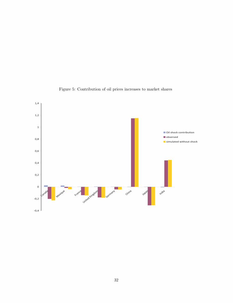
Figure 5: Contribution of oil prices increases to market shares
-0,4
-0,2
0
0,2
0,4
0,6
0,8
1
1,2
1,4
Canada
Mexiq
ue
France
United K
ingdom
Germany
China
Japan
India
Oil shock contribu!on
observed
simulated without shock
32

1999 and 2006, these shares decreased respectively by around 20% and 1.8% and would have
decreased anyway by a bit more (23% and 4%) had the shock never took place. At most, oil
prices have been a factor of small resistance to globalization, but could not contribute at all
to reverse it. Pick India and China as remarkable examples. Their relative share went up
respectively by 44% and 115% over the period. Such figures are extremely high and could easily
resist the very weak (negative) contribution of oil prices (-0.4 and -0.7% respectively).
6 Conclusion
This paper contributes to the debate regarding the effects of oil prices. We study the link with
the geography of trade flows.
Our theoretical idea states that because of the existence of fixed costs, prices of shipping a good
do not respond proportionally to oil prices. This alters the distribution of trade costs and trade
flows among partners: Close countries should benefit from oil shocks at the expense of faraway
countries. This should reverse globalization and leads to a relocation of activities in regional
markets.
We then test this intuition on US bilateral imports data from 1974 to 2001. For a country
located at a median distance to the US, we find a low elasticity of freight rates to oil prices
(around 0.011). The variance of these elasticities across countries’ locations does not appear to
be high neither: we find an elasticity of 0.088 for close to US countries (under 3,000 km) and
0.103 for faraway ones (above 10,000 km). We then apply an estimation strategy to correctly
assess the induced impact on market shares of these countries. We estimate an elasticity value
of relative market shares to oil-prices around 0.013 for close to US countries around -0.004 for
faraway countries. If one considers the sign related to these figures, one can deduce easily that
33

they are consistent with the idea that oil prices are regionalizing trade. But as it stands, the
magnitude of these figures is very small.
To have a better idea of the driving force of regionalism behind oil price increases, we estimate
the contribution of oil prices, in recent years, to changes in the extensive and intensive margins of
the relative shares of US partners. We find that the recent oil price increases from 1999 to 2006
have had a maigre contribution. The oil shock contributed positively to Mexico and Canada’s
export shares by 2.2 to 3 percentage points and had a small if not almost insignificant negative
contribution on India and China’s market shares (between -0.4 to -0.7 percentage points). It
also increased Canada and Mexico’s relative likelihood of exporting by almost similar amounts
(3.5 to 4 percentage points) while leaving Japan, India and China’s exports propensity almost
unaffected with reductions that did not exceed 0.8%
Hence, one should not look anymore at oil prices as if they can contribute extensively at
regionalizing trade. Globalization forces seem much stronger and appear to resist easily to oil
shocks.
A Computation of proportional changes in freight rates for big
oil price changes (price shocks)
Define fr as the freight rate and poil the oil price. Define β′ = β.ln(dist). We can present the
freight equation as follows:
ln(fr) = β′ln(poil) + V
where V represents all other explaining variables.
In period 0, before changes in oil prices, poil, we have the following relation: fr0 = eβ′.ln(poil)0 .eV
34

In period 1, after the oil price change, we have the following relation: fr1 = eβ′.ln(poil)1 .eV .
The growth rate of fr due to a change in oil prices, leaving all other things equal, equals:
dfr
fr=
e(β′.ln(poil)1) − e(β′.ln(poil)0)
e(β′.ln(poil)0)=
((poil)1(poil)0
)β′
− 1
Recall β′ = β.ln(dist). Besides, prices in time 1 are actually the sum of prices in time 0
plus the change in prices that has occurred (i.e. (poil)1 = (poil)0 + dpoil). After removing the 0
subscript we thus obtain:
dfr
fr=
(1 +
dpoil
poil
)β.ln(dist)
− 1
References
Backus, D. and M. Crucini (2000). Oil prices and the terms of trade. Journal of International
Economics 50 (1), 185–213.
Blanchard, O. and J. Gali (2007). The macroeconomic effects of oil price shocks: Why are the
2000s so different from the 1970s? NBER Working Paper 13368 .
Bridgman, B. (2008). Energy prices and the expansion of world trade. Review of Economic
Dynamics 11 (4), 904–916.
Crozet, M., K. Head, and T. Mayer (2009). Quality sorting and trade: Firm-level evidence for
french wine. CEPII Working Paper 2009-14 .
Erkel-Rousse, H. and D. Mirza (2002). Import price elasticities: reconsidering the evidence.
Canadian Journal of Economics 35 (2), 282–306.
35
Feenstra, R. C., J. Romalis, and P. K. Schott (2001). U.s. imports, exports ans tariff data,
1989-2001. NBER Working Paper 9387 .
Hamilton, J. D. (2008). Understanding crude oil prices. NBER Working Paper 14492 .
Hummels, D. (2001). Time as a trade barrier. Purdue University, mimeo.
Hummels, D. (2007). Transportation costs and international trade in the second era of global-
ization. Journal of Economic Perspectives 21 (3), 131–154.
Hummels, D. and A. Skiba (2004). Shipping the good apples out: An empirical confirmation of
the alchian-allen conjecture. Journal of Political Economy 112, 1384–1402.
Rubin, J. and B. Tal (2008). Will soaring transport costs reverse globalization? CIBC World
Market, StrategEcon: The New Inflation.
36