Offshore, Nearshore and Foreshore Behavior of Tsunami Waves

New Mexico High School Adventures in Supercomputing Challenge

Final Report

April 24, 2006

Team Number 121 Advanced Computer Studies

Silver High School, Silver City, NM

Team Members: Ben L. Fox, Junior Richard F. Paul, Sophomore Manuel J. Guadiana, Sophomore Teacher: Mrs. Peggy S. Larisch Mentor: Mr. Berry F. Estes

Acknowledgements The authors wish to acknowledge the following individuals for the guidance provided in the selection of a suitable topic, development of the computer code, adaptation to the computer based analyses, review, and understanding of the results, and assistance provided in the overall preparation of this report:

• Mrs. Peggy S. Larish -Teacher, Silver High School Advanced Computers Studies

• Mr. Berry F. Estes – Nuclear Engineer (Retired), Sandia National Laboratories

• Mr. Harold O. Mofjield – Oceanographer, Pacific Marine Environmental Laboratory/NOAA

2

Table of Contents

E.0 Executive Summary--------------------------------------------------------------- 4 1.0 Introduction -------------------------------------------------------------------------- 5 2.0 Project Proposal-------------------------------------------------------------------- 7 3.0 Analytical Methodology ----------------------------------------------------------- 9 4.0 Results-------------------------------------------------------------------------------- 14 5.0 Conclusion --------------------------------------------------------------------------- 16 6.0 Recommendations for Future Work ------------------------------------------ 18 7.0 References -------------------------------------------------------------------------- 19 8.0 Appendix 1 -------------------------------------------------------------------------- 21 Appendix 2 ------------------------------------------------------------------------- 25 Appendix 3 -------------------------------------------------------------------------- 30 Appendix 4 ------------------------------------------------------------------------- 35 Appendix 5 -------------------------------------------------------------------------- 40

3

E.0 Executive Summary

The purpose of this study is to examine the properties of a tsunami wave and

present the mathematical models of the wave based on the dynamics of a

tsunami that is applicable to promoting an understanding of the energy of a

tsunami.

This report is designed to promote a better understanding of a Tsunami wave.

The mechanics of a tsunami wave are investigated and the mathematical

equations and the physical properties describing a tsunami are developed for the

purpose of examining the wave characteristics and studying the change in the

physical properties (kinetics) of the wave.

The mathematical and physical properties of a tsunami wave are studied for

several representative conditions, and a representative real world tsunami is

simulated through computer modeling.

The project develops a model that has the capability of modeling a variety of

tsunami conditions; the mathematics and the physics of a tsunami wave are

studied through parametric simulations of the behavior of a typical tsunami wave.

The computer program is written using the Excel programming language. The

graphs, equations, and charts for a tsunami are studied to understand and create

a typical model of a tsunami wave. Together with a working model of a tsunami

wave, real time visual representations are outputted using the Excel

programming language.

Through the process of mathematical and graphical representation, a tsunami

wave is presented in classical mathematical format. All calculations and

computer outputs are demonstrated to be correct by hand calculations.

4

1.0 Introduction 1.1 Purpose

Tsunami is a Japanese word that means, “harbor wave”. The word tsunami is

now used to refer to any series of long waves that are generated by a rapid,

large-scale disturbance of the sea floor. The purpose of this study is to examine

the properties of a tsunami wave and present the mathematical models of the

wave based on the dynamics of a tsunami that is applicable to promoting an

understanding of the energy of a tsunami.

This report is designed to promote a better understanding of a Tsunami wave.

The mechanics of a tsunami wave are investigated and the mathematical

equations and the physical properties describing a tsunami are developed for the

purpose of examining the wave characteristics and studying the change in the

physical properties (kinetics) of the wave. These properties include wave

velocity, momentum and total energy Kinetic and potential energies) as the wave

approaches and impacts a shoreline. Typically, a tsunami wave strikes a

shoreline several hours (3-5 hours) after the initial onset of the tsunami. Due to

the localization of tsunamis near a given shoreline, this implies that the superior

response near the shoreline is partly due to localized dynamic properties.

Because of the recent seismic activities that have produced large-scale tsunamis

that impact a coastal environment, a need for a better understanding of a

tsunami wave has arisen. This report develops the total energies and

momentum, and shoreline physical characteristics are reviewed for a spectrum of

representative tsunami waves and beach conditions. The mathematical and physical properties of a tsunami wave are studied for

several representative conditions, and a representative real world tsunami is

simulated through computer modeling.

5

1.2 Scope The project develops a model that has the capability of modeling a variety of

tsunami conditions; the mathematics and the physics of a tsunami wave are

studied through parametric simulations of the behavior of a typical tsunami wave.

The kinetics and momentum, based on selected wave velocity and mass are are

analyzed and discussed for a range of input values.

1.3 Computer Program The computer program is written using the Excel programming language. This

language can perform calculations and store an inventory of variables in arrays.

Information is developed from a variety of sources to gain values for basic

equations of state that are assumed to be applicable throughout the entire

modeled system. This implies that the situations are expected to occur for the

conditions as described. The computer program is capable of selecting specific

data values for a typical tsunami, performing the required calculations and

presents the results in a chart format. The graphs, equations, and charts for a

tsunami are studied to understand and create a typical model of a tsunami wave.

All Excel computations are checked by hand calculations for the purpose of

verifying the accuracy of outputted results and conclusions. Together with a

working model of a tsunami wave, real time visual representations are outputted

using the Excel programming language; these aspects are then coupled with the

Power Point program to display the output in both hard data format and a time

dependent wave motion.

6

2.0 Project Proposal 2.1 Project Description This project investigates a typical mid ocean-produced tsunami by conducting

parametric studies such as wave velocity, and beach characteristics. This

program models wave dynamics and the applicable properties, such as wave

velocity, wave momentum, potential energy, and kinetic energy; the dynamic

behavior of a representative tsunami wave is modeled in both the open ocean

and upon impacting a beach. Obstacles in developing a computational model of

a tsunami wave that yields correct inferences for computer wave mechanics are:

• Identification of required input variables

• Technique for selecting applicable parameters

• Understanding both input and output information

• Developing real time visual representation of the mathematical models.

The computer program is designed to describe a typical tsunami wave and

identifies restrictions on the development of the model such that the mechanics

of the equations produce solutions that describe the physics of a typical tsunami

wave impacting on the nearshore (the zone from the shoreline seaward to the

line of breakers) and a foreshore (the portion of the shore lying between the

normal high an low water marks-the inertial zone) areas.

A technique for enhancing knowledge of the mechanics of a tsunami and a

process for evaluating the overall dynamics is the goal of this project. In order to

achieve this, a comprehensive set of equations is developed that describe the

physics of a tsunami wave, which requires that selective variables be identified

that impact the wave dynamics. Parametric equation operations are performed

7

on each individual variable to determine the overall effect of impact each variable

has on the comprehensive solution.

8

3.0 Analytical Methodology

3.1 Mathematical Bases

The Excel program developed to describe the tsunami behavior employs a

working mathematical model that describes the physical dynamics of a tsunami

wave. These equations describe the mechanics of a wave generated by a large-

scale disturbance of the sea and sea floor and the impact of the wave on a

shoreline.

The Excel computer program displays a real time presentation applying values

calculated using the equations developed in this section to describe the motion of

a wave from time of generation until impact on the foreshore of a coast.

The basic equations used to model a tsunami wave are total energy (TE) and

momentum (P):

• TE=KE+PE

• KE=½*M*V2

• PE=M*g*h

• P=M*V

Where:

• KE=kinetic energy of the wave

• PE=potential energy

• P=momentum of the wave,

• M=mass of the water in a specified volume

• V=wave velocity

• g=gravitational constant

• h=height

9

These equations, as developed, show wave action in relation to real time. The

equations to describe wave motion as a function of time and distance are:

y(t)=Asin2π(x(t)/λ-v/λ*t)

or:

y(t)=Asin2π(x(t)/λ-t/T)

where:

• A=amplitude of the wave (assumed to be 0.5 meters (50 cm) in the open

ocean)

• λ=wave length

• T=period (seconds)

• 1/T=v/λ

• v=wave velocity

• y(t)=vertical position as a function of time

• x(t)=horizontal position as a function of time

These variables represent Tsunami wave input parameters.

3.1.1 Conservation of Energy Wave Impacting a Beach The total energy in a “wave”, that is, a mass of water moving at some specified

velocity consists of two distinct energy components. These are: kinetic energy

and potential energy (refer to Figure 1). The basic equations for the mechanics of

wave motion are given in the preceding Section 3.1. The mechanics of a wave

are examined for two controlled conditions. First, the assumption is made that no

loss of energy occurs, second, loss of energy due to friction at the point of

contact between the wave and the ocean floor.

10

Beach

Total Energy

Potential Energy

Kinetic Energy

Slope of Beach

Figure 1 Energy of Wave

Distance

Ene

rgy

(abs

tract

uni

ts)

11

Two case studies are analyzed; first, no loss of energy, second, loss of energy.

Refer to the appendices for complete analyses of these cases.

3.2 Computer Applications This computer program is designed to enhance the knowledge of the properties

of a tsunami wave. Based on equations for energy and momentum as a function

of time, the computer program outputs solutions for the wave mechanics. The

computer models utilized in this program are based on two basic inputs. First, a

model is developed employing a standard sine function to describe the wave

action with no losses of energy. Throughout the analysis, the assumptions are

made that the total energy, kinetic energy, and potential energies are conserved.

Second, a (future) model is (to be) developed implying that loss of kinetic energy

occurs due to friction.

The Excel program is developed using iterated time steps. This method uses two

rows of cells, creating a circular reference. The first row of cells saves the values

of the function from the last step, and the other row calculates the value of the

function at a new time step. This method allows for a specialized program that

represents a tsunami wave and allows the wave to be displayed in real time.

The program is developed to find a solution to the wave based on several

variables:

• Wave Velocity

• Energy and Momentum

• Mass

• Beach Characteristics- such as slope and depth parameters

All calculations received from the Excel program result in the outputting of the

energy and momentum of the wave in open ocean transit and finally as a function

of beach characteristics. Specifically the program develops solutions as a

12

function of the beach slope and distance of the foreshore of the coast. Graphs

are presented to demonstrate the wave behavior as it impacts and travels up the

beach. The Excel program calculates the energy and momentum values for the

wave as a function of beach characteristics; the equations can be then modified

to employ losses, then the same calculations reiterated and modified

incorporating specified dynamic loss functions to demonstrate the resultant wave

behavior (refer to Section 6.0). Comparisons can be then made between the two

sets of data to represent energy loss and illustrate changes in the waves physical

appearance.

13

4.0 Results The calculations performed by the computer program accurately represent the

properties of a tsunami wave. Calculations also represent the total energies of

the wave and respective relationships between kinetic and potential wave

energy. Parametric equations are constructed to infer conclusions about certain

case conditions. By changing one variable at a time, observations to the different

output values can be made. These calculations are based on the assumption that

the wave shape follows a standard sine function.

4.1 Calculations The computer calculations are shown to be correct by comparing calculations

performed by the computer programs to matching hand calculations. A significant

difficulty encountered in the initial development of the program was the

adaptation of the computer model to accept the input variables:

• Wave velocity

• Wave mass

• Friction factor (between point of contact of water and beach)

• Beach characteristics (depth parameters, beach length, and beach slope)

The computer program utilizes selected complex interrelationships between the

above noted variables; these final relationships are:

• Wave energy

• Wave momentum

• Change of energy states (kinetic and potential)

The equations are developed to show both energy and momentum for a defined

tsunami wave. Refer to the Appendices for complete calculations.

14

4.2 Charts and Figures A Microsoft Excel program is used to calculate the respective equations for wave

energy and momentum. The output (solutions) as a function of selected input

variables are given in Appendices; and special solution for selected energy

losses (refer to Section 3.0) are also presented in two dimensional format as a

function of time for input conditions selected to demonstrate the versatility of the

program.

Figures corresponding to these input/output conditions are created using

Microsoft Excel. The equations describing the time dependent motion of the

wave (refer to section 3.0) are formatted into the Microsoft Excel programming

language to show wave motion as a function of time and demonstrate the

versatility of the program in displaying unique functions.

The figures present several unique conditions (selected especially for this study);

these figures model a representative set of tsunami conditions that demonstrate

the capabilities of this program to show “real time” motion of the wave.

15

5.0 Conclusions 5.1 Mathematical Models Through the process of mathematical and graphical representation, a tsunami

wave is presented in classical mathematical format. All calculations and

computer outputs are demonstrated to be correct by hand calculations.

5.2 Computer Program Calculating the mechanics of the wave requires basic selected inputs, value

parameters characterized as equations of motion in a series of specific

equations. The computer program initially prompts the user to input easily

referenced variables from the reference text and journal articles. Using these

basic variables to specify the unique characterization of the tsunami, the program

selects values from the referenced documents in order to provide the equations

with accurate information on how the wave reacts under the specified input

conditions. These are known as the dynamics of the wave. Combining these

equations and the variable input parameters defined by the user, Excel

calculations are performed to examine wave dynamics for beach characteristics

and wave dynamics (refer to Appendices for complete set of calculations).

5.3 Results The program employs the basic dynamics of wave action to develop solutions for

wave characteristics, in this case a tsunami, as the wave impacts on a specified

shore. Wave action is specified for selected input conditions and resultant output

values are calculated. Purpose of these calculations is to demonstrate that a set

of output can be correctly determined for a specified set of input conditions (in

this case, a defined tsunami wave), and the calculated values for energy and

momentum can be employed to characterize wave behavior.

16

5.4 Word Processor Program The written portion of the program is created using Microsoft Word; the

calculations are performed using a modified Excel program for the purpose of

displaying the tsunami wave in real time motion.

17

6.0 Recommendations for Future Work To improve the project beyond what has been accomplished to date, it is

recommended that improvements be made on the cross section view of a

specified tsunami wave for a larger wave section. The program should also be

written to represent a plan view of the wave and a specified coastline. Loss of

energy and changes in wave characteristics due to reflection, refraction and

energy loss, and deflection should also be added to represent more realistic

behavior.

18

7.0 References 1. Gonzàlez, F.I., K. Satake, E.F. Boss, H. O. Mofjeld. Edge Wave and Non-

Trapped Modes of the 25 April 1992 Cape Mendocino Tsunami.

2. Mofjeld, H.O., V.V. Titov, F.I. Gonzàlez, J.C. Newman. Analytic Theory of

Tsunami Wave Scattering in the Open Ocean with Application to

the North Pacific. NOAA Technical Memorandum OAR PMEL-116.

January 2000.

3. Thurman, Harold V. Introductory Oceanography. Columbus: Bell & Howell,

1975.

19

8.0 Appendices

20

Appendix 1

Equations to Describe Wave Motions as a Function of Time

21

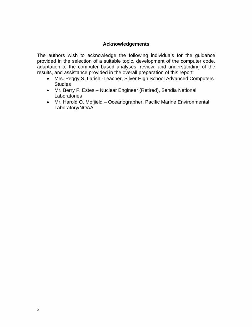
These equations describe wave motion as a function of time. The following

equation describes the basic for of wave motions.

y(t)=Asin2π(x(t)/λ-v/λ*t)

or:

y(t)=Asin2π(x(t)/λ-t/T)

For tsunami wave input parameter:

• = wave length = 400 m = 40,000 cm.

• T = period (seconds)

• I/t = v/λ = 1670/40000 = 0.042 sec-1

• V = wave velocity = 600 km/hr = 600000/3600 = 16700 cm/sec

• Y(t) = vertical position as a function of time (cm)

• X(t) = horizontal position as a function of time (cm)

Substituting these values: into the equation for y(t), the vertical displacement of

the wave as a function of horizontal distance is:

Y(t) = A sin 2π (x(t)/40000 – 16700/40000 * T)

= A sin 2π (x(t)/40000 0.42 T)

The amplitude of the wave is given by A and for this example the wave height

(amplitude) is assumed to b 0.40 meters or 40 cm.

Y(t) = 40 2π (x(t)/40000 0.42 T)

= 40 2π (1.57 * 10-4 x(t) – 2.62T)

22

This equation describes the vertical displacement (or motion) of the wave as a

function of time and downrange position – x(t).

As example, assumes the a following value, for x(t) and t:

• X(t)= 10000 cm.

• T(t)= 100sec.

The vertical displacement of the wave is.

Y(t) = 40 Sin [ 1.57-4 * (10000) – 2.62 (100)]

= 40 Sin [1.57 - 262.0]

=(-260.4)

Where the argument of the sine function is in radians, solving for y(t).

Y(t) = [40 0.317]

=12.67 cm

In other words, at the specified time (100 seconds) and downrange distance

(10000cm) the height of the wave is 12.67cm for the assumed input conditions.

The vertical velocity of the wave can be determined by differentiating the basic

equations for y(t).

y(t) = 40 sin [1.57 x 10-4 (x(t)) –2.62t]

dy(t)/dt = vertical velocity =Vv(t)

=d {40 sin [1.57 x 10-4 (x(t)) –2.62t]}/ dt

The variable to be differentiated is 2.62t since that is the term containing time as

a variable, thus:

dy (t)/dt = Vv (t)

23

= 40 {-2.62{cos[(1.57 x 10-4 (10000) –2.62 t(t)]}}

= -104.80{cos[1.57 x 10-4 x (t) –2.62 t (t)]}

Substituting the ordinal assumed value: for x (t) and t(t) [x(t) = 10000cm and t(t)

= 100sec] the vertical or transverse wave velocity is

Vv(t) = -104.80 {cos[1.57 x 10-4 (10000) –2.62 (100)]}

= -104.80 cos [ 1.57 – 2.62]

= -104.80 cos (-260.43)

= -104.80 (-0.948)

= 99.4 cm/sec ( upward w/repeat to horizontal plane )

[ Note : A minus sign would indicate a downward velocity]

Consequently, for the assumed input conditions, at a downrange distance of x(t)

= 10000cm, time t(t) = 100sec, the following conditions of wave are:

y(t) = 12.67 cm

x(t) = 10000 cm

v(t) = 16700 cm/sec

vv(t) = 99.4 cm/sec

24

Appendix 2

Conservation of Energy Wave Impacting a Beach

25

The total energy in a “wave”, that is mass of water moving at some specified

velocity consists of two distinct energy components. There are kinetic energy and

potential energy. The mechanics of a wave is presented below for the condition

of no energy losses [a follow-on study is planned to examine energy loss due to

friction between the wave (or mass of water) and the ocean floor (as it rises to

the beach level)]. A plot of these two terms is represented in Figure 1.

Total energy in wave Start of beach Potential energy Underwater Slope Kinetic Energy E

nerg

y (a

rbitr

ary

units

)

Distance of Slope of Beach Figure 1- Energy of Wave

As illustrated in Figure 1 (which is a hypothetical representation of the energy

distribution), as the wave enters the zone of the below-surface region (0 – x), the

kinetic energy and the potential energy change in magnitude but for the no-loss-

of-energy condition the total energy remains constant. This is analyzed in the

following section .

No Loss of Energy

26

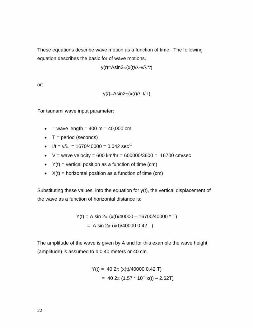
A slug of water is assumed to encounter the bottom or leading edge of the

submerged beach as shown in Figure 2.

Sea level

L

d

θ Reference

plane h h

The mass of water in the elemental volume, ΔV, is given by:

Mass of water = m w = ρsw * vol. of sample slug

= ρsw * h t w

Where w is the width of the slug of water but for purposes of this analysis it is

assumed to be of unit length (that is,1) so that the mass of water can be re-

written as:

m w = ρsw * h t

The kinetic energy of the slug of water is given by:

KE slug = ½ m * v2

Where v = the velocity of the slug of water as is travels up the slope.

The potential energy of the slug of water is given by:

PE = mg H

27

Where H is the height of the center of mass of the slug above the reference

plane. Since the water mass is assumed uniform and dimensionally constant, the

potential energy can be written in terms of total sub – surface height h as:

PE= ½ mgh

As previously noted, the total energy of the wave is assumed too remain constant

(for care 1); hence

Total Energy (TE) = Kinetic Energy (KE) + potential energy

(PE)

Or TE = KE + PE

And substituting for these terms:

TE = ½ mv2 + ½ mgh

Next, the solution must account for the underwater slope of the beach, or angle

θ. Introducing the change in height of the slug of water as it traverses up the

underwater slope, the term for h is modified as follows:

H = L sin θ

This term allows the equation to account for the length or “run” of the underwater

distance the slug of water travels as is rises to the top of the beach. Also, the

down-range distance d, which is the horizontal distance the wave travels as the

wave travels up the slope of the beach is given by:

d = L cos θ

or using another expression

d = h / tan θ

28

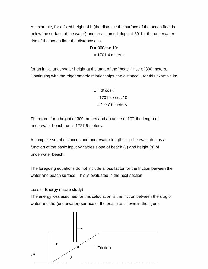
As example, for a fixed height of h (the distance the surface of the ocean floor is

below the surface of the water) and an assumed slope of 30o for the underwater

rise of the ocean floor the distance d is:

D = 300/tan 10o

= 1701.4 meters

for an initial underwater height at the start of the “beach” rise of 300 meters.

Continuing with the trigonometric relationships, the distance L for this example is:

L = d/ cos θ

=1701.4 / cos 10

= 1727.6 meters

Therefore, for a height of 300 meters and an angle of 10o; the length of

underwater beach run is 1727.6 meters.

A complete set of distances and underwater lengths can be evaluated as a

function of the basic input variables slope of beach (θ) and height (h) of

underwater beach.

The foregoing equations do not include a loss factor for the friction beween the

water and beach surface. This is evaluated in the next section.

Loss of Energy (future study)

The energy loss assumed for this calculation is the friction between the slug of

water and the (underwater) surface of the beach as shown in the figure.

29

Friction

θ

Appendix 3

Review of the Total Energy In the Wave

30

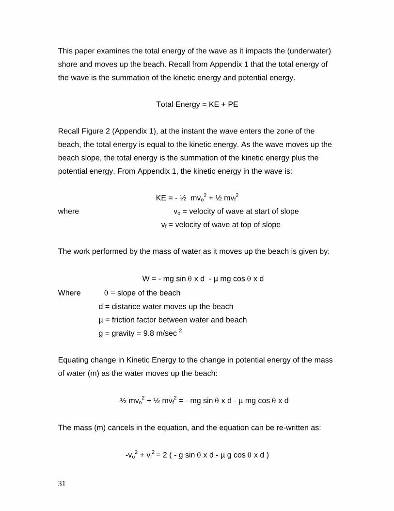
This paper examines the total energy of the wave as it impacts the (underwater)

shore and moves up the beach. Recall from Appendix 1 that the total energy of

the wave is the summation of the kinetic energy and potential energy.

Total Energy = KE + PE

Recall Figure 2 (Appendix 1), at the instant the wave enters the zone of the

beach, the total energy is equal to the kinetic energy. As the wave moves up the

beach slope, the total energy is the summation of the kinetic energy plus the

potential energy. From Appendix 1, the kinetic energy in the wave is:

KE = - ½ mvo2 + ½ mvf

2

where vo = velocity of wave at start of slope

vf = velocity of wave at top of slope

The work performed by the mass of water as it moves up the beach is given by:

W = - mg sin θ x d - µ mg cos θ x d

Where θ = slope of the beach

d = distance water moves up the beach

µ = friction factor between water and beach

g = gravity = 9.8 m/sec 2

Equating change in Kinetic Energy to the change in potential energy of the mass

of water (m) as the water moves up the beach:

-½ mvo2 + ½ mvf

2 = - mg sin θ x d - µ mg cos θ x d

The mass (m) cancels in the equation, and the equation can be re-written as:

-vo2 + vf

2 = 2 ( - g sin θ x d - µ g cos θ x d )

31

The velocity vf at the top of the beach is:

vf2 = vo

2 - 2gd ( sin θ + µ cos θ)

Divide by cos θ and rearranging terms:

vf2 = vo

2 - 2gd cos θ (µ + tan θ)

or

vf = [vo2 – 2gd cos θ ( µ + tan θ)] ½

This equation describes the velocity of the wave as the wave moves up the

underwater beach of slope “θ”. If, as example, it is assumed that there is no

friction, that is µ = 0, the above equation reduces to:

Vf = [ vo2 – 2gd sin θ ] ½

As shown in Appendix 1 for an assumed set of input conditions, namely:

D = 300/sinθ = 300/sin10o = 1727.6 m.

θ = 10*

µ = 0.01

Vf = [(166.67)2 – 2(9.8)(1727.6)(cos10o)(0.01 + tan 10o)]½

= 146.9 m/sec.

This is the velocity or the water ( or wave front ) as it reaches the end of the

underwater beach.

32

The change in Kinetic Energy of the wave is given by :

KE = KE @ start – KE @ top

= ½ mvo2 – ½ mvi

2

= ½ m [(166.7)2 – (146.9)2]

= m x 3106.7 Joules

This represent the LOSS in Kinetic Energy as the wave proceeds up the

underwater beach. This value also represents the change in potential energy

which can be equated to the change in Kinetic Energy. The change in potential

energy is given by

PE = mgd sin θ + µ mgd cos θ

= m(9.8)(1727.6)[sin 10o + 0.01 cos 10o]

= m x 3106.7 Joules

This basically agrees with the KE term above.

If there is no friction factor assumed then the change in the Potential Energy

(PE) in given by:

PE = mgd sinθ

And the final velocity at the top of the underwater beach is given by:

- vo2 + vf

2 = - 2dg sinθ

or:

vf2 = vo

2 –2dg sinθ

= [(166.67)2 – 2 (9.8)(1727.6) sin10o]

33

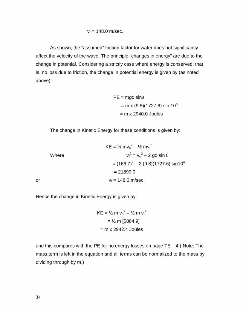
vf = 148.0 m/sec.

As shown, the “assumed” friction factor for water does not significantly

affect the velocity of the wave. The principle “changes in energy” are due to the

change in potential. Considering a strictly case where energy is conserved, that

is, no loss due to friction, the change in potential energy is given by (as noted

above):

PE = mgd sinθ

= m x (9.8)(1727.6) sin 10o

= m x 2940.0 Joules

The change in Kinetic Energy for these conditions is given by:

KE = ½ mvo2 – ½ mvf

2

Where vf2 = vo

2 – 2 gd sin θ

= (166.7)2 – 2 (9.8)(1727.6) sin10o

= 21899.0

or vf = 148.0 m/sec.

Hence the change in Kinetic Energy is given by:

KE = ½ m vo2 – ½ m vf

2

= ½ m [5884.9]

= m x 2942.4 Joules

and this compares with the PE for no energy losses on page TE – 4 ( Note: The

mass term is left in the equation and all terms can be normalized to the mass by

dividing through by m.)

34

Appendix 4

Excel Calculations

35

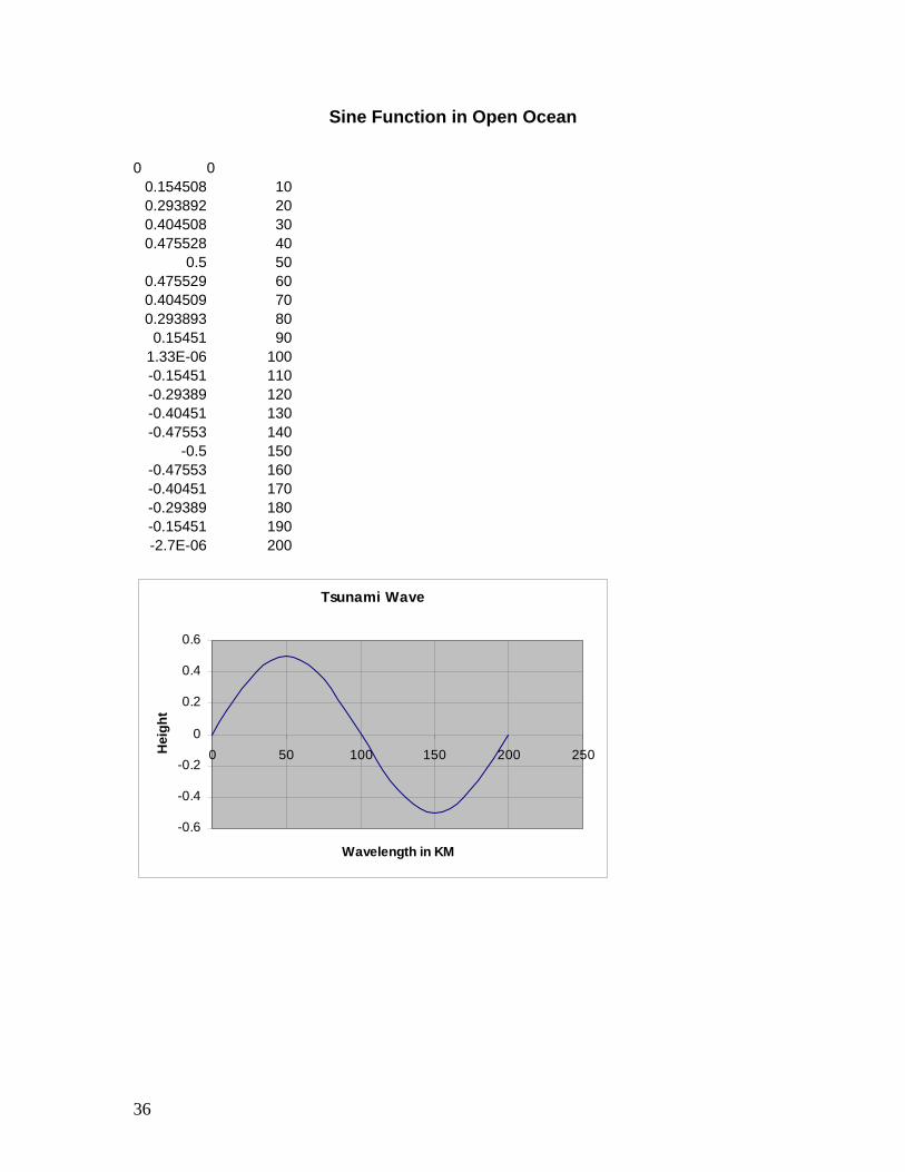
Sine Function in Open Ocean 0 0

0.154508 100.293892 200.404508 300.475528 40

0.5 500.475529 600.404509 700.293893 80

0.15451 901.33E-06 100-0.15451 110-0.29389 120-0.40451 130-0.47553 140

-0.5 150-0.47553 160-0.40451 170-0.29389 180-0.15451 190-2.7E-06 200

Tsunami Wave

-0.6

-0.4

-0.2

0

0.2

0.4

0.6

0 50 100 150 200 250

Wavelength in KM

Hei

ght

36

Wave Behavior (Impacting Beach)

10 Beach Slope

0.174533 0 0 0

85.06923 15.00188 15.15639170.1385 29.98863 30.28252255.2077 44.94661 45.35112340.2769 59.865 60.34053425.3461 74.73684 75.23684510.4154 89.55974 90.03527595.4846 104.3361 104.7406680.5538 119.0728 119.3667

765.623 133.7808 133.9353850.6923 148.4737 148.4737935.7615 163.1665 163.0121020.831 177.8745 177.5806

1105.9 192.6113 192.20681190.969 207.3876 206.91211276.038 222.2105 221.71051361.108 237.0824 236.60681446.177 252.0008 251.59621531.246 266.9587 266.66481616.315 281.9455 281.7911701.385 296.9474 296.9474

Wave Behavior (1 degree slope)

050

100150200250300350

0 500 1000 1500 2000

Beach Length

Wav

e H

eigh

t

Series1 Series2

37

100 Beach Slope

0.017453 0 0 0

859.451 15.15474541 15.309251718.902 30.29436649 30.588262578.353 45.40521938 45.809733437.804 60.47647625 60.9524297.255 75.5011852 76.001195156.706 90.47695074 90.952486016.157 105.4061683 105.81076875.608 120.2957898 120.58977735.059 135.156643 135.3112

8594.51 150.0023717 150.00249453.961 164.8481003 164.693610313.41 179.7089531 179.415111172.86 194.598574 194.194112032.31 209.5277909 209.052312891.77 224.5035556 224.003613751.22 239.5282637 239.052714610.67 254.5995198 254.19515470.12 269.7103722 269.416516329.57 284.8499929 284.695517189.02 300.0047381 300.0047

Wave Behavior (10 degree slope)

050

100150200250300350

0 5000 10000 15000 20000

Beach Length

Wav

e H

eigh

t

Series1 Series2

38

Wave Momentum and Kinetic Energy Calculations Velocity Km/hr velocity m/sc KE in MKS KE in Enginering Mass in MKS Velocity in ft/sc

600 166.67 4.26E+10 1.01E+12 3066000 546.92620 172.22 4.55E+10 1.08E+12 3066000 565.15640 177.78 4.85E+10 1.15E+12 3066000 583.39660 183.33 5.15E+10 1.22E+12 3066000 601.62680 188.89 5.47E+10 1.30E+12 3066000 619.85700 194.44 5.80E+10 1.37E+12 3066000 638.08720 200.00 6.13E+10 1.45E+12 3066000 656.31740 205.56 6.48E+10 1.53E+12 3066000 674.54760 211.11 6.83E+10 1.62E+12 3066000 692.77780 216.67 7.20E+10 1.70E+12 3066000 711.00800 222.22 7.57E+10 1.79E+12 3066000 729.23820 227.78 7.95E+10 1.88E+12 3066000 747.46840 233.33 8.35E+10 1.98E+12 3066000 765.69860 238.89 8.75E+10 2.07E+12 3066000 783.92880 244.44 9.16E+10 2.17E+12 3066000 802.15900 250.00 9.58E+10 2.27E+12 3066000 820.39

velocity m/sc Momentum in MKS

166.67 5.11E+08172.22 5.28E+08177.78 5.45E+08183.33 5.62E+08188.89 5.79E+08194.44 5.96E+08200.00 6.13E+08205.56 6.30E+08211.11 6.47E+08216.67 6.64E+08222.22 6.81E+08227.78 6.98E+08233.33 7.15E+08238.89 7.32E+08244.44 7.49E+08250.00 7.67E+08

39

Appendix 5 Excel Program

Typical Sine Function

40

Time 1.00Init Flag TRUE

1 -1.00

0 -0.0975451 10 0.0587686 20 0.2093297 30 0.3394001 40 0.4362478 50 0.4903925 60 0.4965343 70 0.4540719 80 0.3671619 90 0.2443116 100 0.0975464 110 -0.0587673 120 -0.2093285 130 -0.3393992 140 -0.4362471 150 -0.4903923 160 -0.4965345 170 -0.4540725 180 -0.3671628 190 -0.2443127 200 -0.0975477

Sin Function Model

-0.6000000

-0.4000000

-0.2000000

0.0000000

0.2000000

0.4000000

0.6000000

0 50 100 150 200 250

41