Embed Size (px)
Citation preview

Technological University Dublin Technological University Dublin
ARROW@TU Dublin ARROW@TU Dublin
Doctoral Engineering
2015-4
Offshore Electrical Networks and Grid Integration of Wave Energy Offshore Electrical Networks and Grid Integration of Wave Energy
Converter Arrays - Techno-economic Optimisation of Array Converter Arrays - Techno-economic Optimisation of Array
Electrical Networks, Power Quality Assessment, and Irish Market Electrical Networks, Power Quality Assessment, and Irish Market
Perspectives Perspectives
Fergus Sharkey Technological University Dublin, [email protected]
Follow this and additional works at: https://arrow.tudublin.ie/engdoc
Part of the Other Electrical and Computer Engineering Commons, and the Power and Energy
Commons
Recommended Citation Recommended Citation Sharkey, F. (2015). Offshore Electrical Networks and Grid Integration of Wave Energy Converter Arrays - Techno-economic Optimisation of Array Electrical Networks, Power Quality Assessment, and Irish Market Perspectives. Doctoral Thesis. Technological University Dublin. doi:10.21427/D7VG7F
This Theses, Ph.D is brought to you for free and open access by the Engineering at ARROW@TU Dublin. It has been accepted for inclusion in Doctoral by an authorized administrator of ARROW@TU Dublin. For more information, please contact [email protected], [email protected].
This work is licensed under a Creative Commons Attribution-Noncommercial-Share Alike 4.0 License

Offshore Electrical Networks and Grid
Integration of Wave Energy Converter Arrays Techno-economic Optimisation of Array Electrical Networks, Power
Quality Assessment, and Irish Market Perspectives
Fergus Sharkey, BEng
A thesis submitted for the Doctor of Philosophy
to the Dublin Institute of Technology
Supervised by
Prof. Michael Conlon and Mr. Kevin Gaughan
School of Electrical and Electronic Engineering
Dublin Institute of Technology
Kevin Street
Dublin 8
April 2015

i

ii
Abstract
Wave energy is an emerging industry and faces many challenges before commercial
wave energy converter (WEC) arrays are installed. One of these challenges is the grid
integration of WEC arrays. This includes offshore electrical networks, grid compliance, and
access to electrical markets. This must be achieved in a technically viable manner and also at
an acceptable cost. As electrical networks are expected to make up a large proportion of the
overall WEC array CAPEX, perhaps up to 25%, this area is critical to the long term
competitiveness of wave energy.
The objectives of this thesis are to develop technically and economically acceptable
electrical network designs for WEC arrays, evaluate voltage flicker issues for WEC arrays
and develop design tools to analyse same, and evaluate the market scale for wave energy in
Ireland, considering electrical integration issues in both the domestic and export markets.
This thesis presents the optimum design for WEC array electrical networks. By
building from the industry state of the art, including offshore wind experience, a
comprehensive techno-economic optimisation process is undertaken. This includes
optimising the key electrical interfaces between the WEC and the array electrical network,
optimising the array network configuration, assessing efficiency of the network, and
demonstrating that the network can be achieved at a cost which will allow competitiveness.
Some challenges to the economics of WEC array electrical networks and some strategies for
improving the economics are presented in this research also. The results provide timely
guidance to WEC and WEC array developers.
This research also demonstrates the critical link between voltage flicker emissions
from WECs and the primary resource, i.e. ocean waves. Some practical assessment tools for
the evaluation of this power quality issue are shown to assist in quantifying the problem.
Also the full flicker performance of a candidate WEC is assessed helping characterise this
link further.
In this thesis both the domestic and export markets for Ireland’s wave energy resource
are assessed as, although Ireland has an enviable wave energy resource, it is unclear where
the market for this resource lies. This analysis shows that the medium term market for wave

iii
energy in Ireland is an export market. Also, although technically feasible, there is an
additional cost for export transmission which must be considered in evaluating export
markets.
Some of the critical grid integration issues have been evaluated and addressed in this
thesis. Future work is recommended in the areas of weather risk to cable installation at high
energy wave sites, evaluating the benefits of shared electrical infrastructure across a range of
renewable projects, designing offshore substations for WEC arrays, and quantifying the
benefits of the addition of wave energy to the Irish renewable energy mix.

iv
Declaration
I certify that this thesis which I now submit for examination for the award of Doctor of
Philosophy, is entirely my own work and has not been taken from the work of others save and
to the extent that such work has been cited and acknowledged within the text of my work.
This thesis was prepared according to the regulations for post graduate study by research of
the Dublin Institute of Technology and has not been submitted in whole or part for an award
in any other Institute or University.
The work reported on in this thesis conforms to the principles and requirements of the
Institute’s guidelines for ethics in research.
The Institute has permission to keep, to lend or to copy this thesis in whole or in part, on
condition that any such use of the material of the thesis be duly acknowledged.
Signature______________________________________ Date________________________
Candidate

v

vi
Acknowledgements
It is with the utmost pleasure that I submit my PhD thesis. I have undertaken an
incredible journey by completing this work and have emerged as a better engineer and more
critical thinker. I can’t imagine how I would have reached this stage without the help and
support of the below people. I simply cannot express my gratitude enough.
My wife, Jen, has been a constant support and cheerleader for me over the course of
this research. She is always by my side, and I owe her so much. She is also a great proof-
reader; I just hope I haven’t bored her too much! My family, the Sharkeys and the Murphys,
have also kept me motivated and egged me onwards when the going got tough. I’d also like
to thank my good friends, Eoin and John, for persevering with proofing this text.
My supervisors in DIT, Michael and Kevin, have been extraordinarily supportive
from the moment I approached them about this research. I have taken a huge amount from
our regular meetings, and I appreciate the forthrightness and good humour that characterised
our work together. I also acknowledge the assistance that Kevin Honer provided to the work
presented in Chapter 7 of this thesis.
Within ESB I have had tremendous support from across the organisation and feel
privileged to have been allowed to pursue this ambition while working. I particularly want to
thank John Fitzgerald for encouraging me to take on this challenge, providing guidance, and
for the flexibility he has afforded me to complete it. Put simply, I would not have achieved
this without him. I also want to thank Mick Mackey, Michael Quigley, Colm deBurca,
Brendan Barry, and Cera Slevin for their support for this research. Joe MacEnri, ex-ESB,
contributed a lot of his time to assist my understanding of power quality and his expertise and
guidance was much appreciated.
From 2009 to 2011 I was seconded to Wavebob Ltd., a wave energy technology
development company. The work that I began with this company contributed massively to
this body of research. I would specifically like to thank Andrew Parish, then CEO of
Wavebob, and Elva Bannon, for her massive contribution and MatLab expertise.

vii
viii
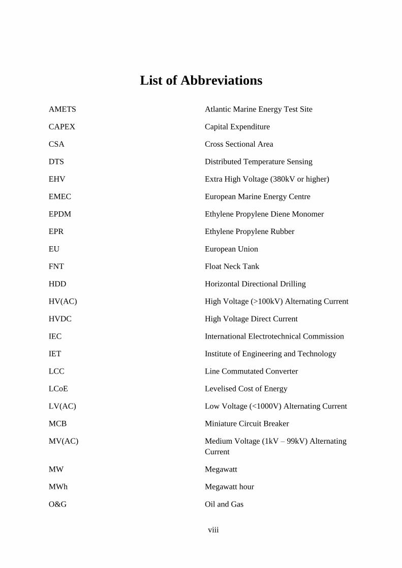
List of Abbreviations
AMETS Atlantic Marine Energy Test Site
CAPEX Capital Expenditure
CSA Cross Sectional Area
DTS Distributed Temperature Sensing
EHV Extra High Voltage (380kV or higher)
EMEC European Marine Energy Centre
EPDM Ethylene Propylene Diene Monomer
EPR Ethylene Propylene Rubber
EU European Union
FNT Float Neck Tank
HDD Horizontal Directional Drilling
HV(AC) High Voltage (>100kV) Alternating Current
HVDC High Voltage Direct Current
IEC International Electrotechnical Commission
IET Institute of Engineering and Technology
LCC Line Commutated Converter
LCoE Levelised Cost of Energy
LV(AC) Low Voltage (<1000V) Alternating Current
MCB Miniature Circuit Breaker
MV(AC) Medium Voltage (1kV – 99kV) Alternating
Current
MW Megawatt
MWh Megawatt hour
O&G Oil and Gas

ix
OPEX Operational Expenditure
OPT Ocean Power Technologies
OSS Offshore Sub-station
OWC Oscillating Water Column
PMG Permanent Magnet Generator
POC Point of Connection
PTO Power Take Off
RES Renewable Energy Source
RMU Ring Main Unit
ROV Remotely Operated Vehicle
RTTR Real Time Thermal Rating
SCIG Squirrel Cage Induction Generator
SEAI Sustainable Energy Authority of Ireland
SEM Single Electricity Market
SNSP System Non-Synchronous Penetration
VSC Voltage Source Converter
WEC Wave Energy Converter
WTG Wind Turbine Generator
XLPE Crossed Linked Polyethylene

x
Contents
Abstract .......................................................................................................................... ii
Declaration .................................................................................................................... iv
Acknowledgements ....................................................................................................... vi
List of Abbreviations ................................................................................................. viii
List of Figures .......................................................................................................... xviii
List of Tables .............................................................................................................. xxi
1. Introduction .......................................................................................................... 1
1.1 Research Problem ............................................................................................. 1
1.1.1 Research Objectives ................................................................................... 2
1.1.2 Novel Academic Contribution, and Technologic Advances in this Thesis 3
1.1.3 Thesis Outline ............................................................................................ 4
1.1.4 Status of the Wave Energy Industry ........................................................... 6
1.1.5 Experience and Plans for WEC Arrays ...................................................... 6
1.1.6 The European and Irish Energy Market ..................................................... 8
1.1.7 Competitive Wave Energy ......................................................................... 9
1.2 Wave Energy Introduction ............................................................................. 10
1.2.1 The Wave Energy Resource ..................................................................... 13
1.2.2 Conversion of Wave Energy into Electrical Energy ................................ 14
1.3 Wave Energy Converters ............................................................................... 15
1.3.1 WEC Types .............................................................................................. 15
1.3.2 Wavebob................................................................................................... 22
2 Literature Review .................................................................................................. 23
2.1 Introduction .................................................................................................... 23
2.2 Notable Publications ...................................................................................... 24
2.3 Generators for Wave Energy Converters ....................................................... 25

xi
2.4 Grid Integration of Wave Energy ................................................................... 26
2.5 Power Quality and Energy Storage ................................................................ 28
2.6 WEC Array Electrical Networks .................................................................... 29
2.7 Offshore Wind Electrical Networks & Economics ........................................ 32
2.8 Array Layout .................................................................................................. 33
2.9 Dynamic Rating.............................................................................................. 33
2.10 Literature Review Summary ....................................................................... 34
3 State of the Art in WEC Array and Offshore Wind Electrical Networks .............. 35
3.1 Introduction .................................................................................................... 35
3.2 WEC On-Board Electrical Systems ............................................................... 36
3.2.1 Generators ................................................................................................ 36
3.2.2 Switchgear and Protection ........................................................................ 41
3.2.3 Transformers ............................................................................................ 42
3.3 WEC Array Electrical Components ............................................................... 45
3.3.1 Submarine Cables ..................................................................................... 45
3.3.2 Submarine Connectors ............................................................................. 49
3.3.3 Submarine Electrical Equipment .............................................................. 52
3.3.4 Offshore Substations ................................................................................ 57
3.4 WEC Test Sites and Electrical Infrastructure ................................................ 57
3.4.1 European Marine Energy Centre (EMEC) ............................................... 58
3.4.2 Atlantic Marine Energy Test Site (AMETS)............................................ 60
3.4.3 Wavehub................................................................................................... 61
3.4.4 Other Test Sites ........................................................................................ 63
3.5 WEC Prototype Electrical Infrastructure ....................................................... 66
3.5.1 Aguçadoura Wave Farm........................................................................... 66
3.5.2 AW Energy at Peniche ............................................................................. 67
3.5.3 Seabased at Lysekil .................................................................................. 67
xii
3.5.4 Ocean Power Technologies ...................................................................... 69
3.6 Offshore Wind Electrical Networks and Transfer to WEC Arrays ................ 70
3.6.1 Offshore Wind Electrical Networks ......................................................... 70
3.6.2 Array Configuration and Protection ......................................................... 72
3.6.3 Redundancy and Sectionalising ............................................................... 77
3.6.4 Submarine Cable Installation ................................................................... 78
3.6.5 Offshore Substations ................................................................................ 81
3.6.6 HVDC Transmission for Offshore Wind ................................................. 83
3.6.7 Efficiency of Offshore Wind Collection and Transmission Systems ...... 86
3.7 Crossover and Differences between Offshore Wind Farms and WEC Array
Electrical Networks .............................................................................................................. 86
3.8 Conclusion ...................................................................................................... 88
4 Techno-economic Analysis of Electrical Networks for WEC Arrays ................... 89
4.1 Introduction .................................................................................................... 89
4.1.1 Technical, Functional and Economic Factors .......................................... 89
4.1.2 Methodology ............................................................................................ 90
4.2 Wave Energy Cost Breakdown and Target Cost ............................................ 93
4.3 WEC Array Design Considerations, Constraints and Assumptions .............. 94
4.3.1 The Wavebob Wave Energy Converter ................................................... 94
4.3.2 Site Locations ........................................................................................... 95
4.3.3 Resource and Generation Distribution ..................................................... 96
4.3.4 Array Spatial Configuration ..................................................................... 98
4.3.5 Generators .............................................................................................. 100
4.3.6 Dynamic Cables ..................................................................................... 100
4.3.7 Target Electrical Network Efficiency .................................................... 101
4.3.8 Availability ............................................................................................. 101
4.3.9 Cable Losses ........................................................................................... 102

xiii
4.3.10 Cable Selection and Calculation .......................................................... 104
4.3.11 Cable Parameters .................................................................................. 104
4.3.12 Cable Cost Model ................................................................................. 105
4.3.13 WEC Array Capacity ........................................................................... 119
4.4 Key Electrical Interfaces .............................................................................. 120
4.4.1 Dynamic Cable to WEC Interface .......................................................... 122
4.4.2 Dynamic Cable to Static Cable Interface ............................................... 124
4.4.3 WEC MV Switchgear Interface ............................................................. 127
4.4.4 Offshore Substation ................................................................................ 130
4.4.5 Submarine Hubs and Substations ........................................................... 131
4.5 Array Electrical Network Configuration Evaluation ................................... 132
4.5.1 Simple Radial (A)................................................................................... 134
4.5.2 Single Return Ring (B) ........................................................................... 136
4.5.3 Single Sided Ring (C) ............................................................................ 138
4.5.4 Double Sided Ring (D) ........................................................................... 139
4.5.5 Star Cluster (E) ....................................................................................... 141
4.5.6 Overcoming Radial Limitations ............................................................. 143
4.6 Techno-Economic Optimisation .................................................................. 145
4.6.1 Least Cost Solution ................................................................................ 145
4.6.2 Maximum Functionality Solution .......................................................... 146
4.6.3 Optimised Solution ................................................................................. 147
4.7 Array Voltage and Efficiency Analysis ....................................................... 149
4.7.1 WEC Array 1 .......................................................................................... 149
4.7.2 WEC Array 2 .......................................................................................... 156
4.7.3 WEC Array 3 .......................................................................................... 160
4.7.4 Summary ................................................................................................ 165
4.8 Achieving CAPEX Targets .......................................................................... 166

xiv
4.9 Conclusion .................................................................................................... 167
5 Economic Challenges and Cost Reduction Strategies for WEC Array Electrical
Networks 171
5.1 Introduction .................................................................................................. 171
5.2 Economic Challenges for WEC Array Electrical Networks ........................ 171
5.2.1 Redundancy and Star Cluster Networks................................................. 172
5.2.2 WEC Array Spacing ............................................................................... 173
5.2.3 Individual WEC ratings .......................................................................... 173
5.2.4 Device Capacity Factor .......................................................................... 174
5.2.5 Submarine Connectors and other Submarine Electrical Systems .......... 176
5.2.6 Array and Export Voltage ...................................................................... 176
5.2.7 Cable Installation and Export Distance .................................................. 178
5.2.8 WEC Dynamic Response ....................................................................... 179
5.3 Maximising Value from WEC Array Electrical Networks .......................... 180
5.3.1 Strategies for Maximising Value of WEC Array Electrical Networks .. 180
5.3.2 Detailed Analysis and Results ................................................................ 183
5.4 Conclusion .................................................................................................... 196
6 Resource Induced Flicker Assessment for Wave Energy Converters ................. 199
6.1 Introduction .................................................................................................. 199
6.1.1 Power Quality and Flicker...................................................................... 200
6.1.2 IEC Existing and Emerging Power Quality Standards........................... 202
6.1.3 Rationale for Flicker Assessment Tool .................................................. 203
6.2 Wave Energy Resource Induced Flicker ...................................................... 203
6.2.1 Flicker Curve .......................................................................................... 203
6.2.2 Voltage Flicker Emission from Wave Energy Converters ..................... 204
6.3 Flicker Assessment ....................................................................................... 205
6.3.1 Basic Flicker Assessment ....................................................................... 205

xv
6.3.2 Flicker Assessment Tool ........................................................................ 205
6.3.3 Examples of Flicker Assessment Chart Use .......................................... 210
6.3.4 Flicker Measurement Standards ............................................................. 211
6.4 Case Study: Wavebob .................................................................................. 213
6.4.1 Basic Flicker Assessment ....................................................................... 213
6.4.2 Flicker Assessment Charts ..................................................................... 213
6.4.3 Full Flicker Assessment ......................................................................... 214
6.5 Array Cancellation Effect............................................................................. 217
6.6 Flicker Mitigation ......................................................................................... 218
6.6.1 Energy Storage/Smoothing: ................................................................... 218
6.6.2 Spatial Configuration (Cancellation Effect) ........................................... 218
6.6.3 Control Strategy ..................................................................................... 219
6.6.4 Reactive Power Compensation............................................................... 219
6.6.5 Increasing Short Circuit Power .............................................................. 219
6.7 Conclusion .................................................................................................... 220
7 The Domestic and Export Market for Irish Wave Energy................................... 221
7.1 Introduction .................................................................................................. 221
7.2 Wave Energy Resource and Location in Ireland .......................................... 221
7.3 Hypothetical WEC Arrays for Analysis ....................................................... 222
7.4 2020 Targets and Wind Development in Ireland ......................................... 224
7.5 Wave Energy Opportunities in the Irish Market .......................................... 226
7.5.1 Non-Concurrence and Diversity............................................................. 226
7.5.2 Additional Interconnection and Storage in the System .......................... 227
7.5.3 Re-use of redundant infrastructure. ........................................................ 227
7.5.4 Synchronous Wave Energy Converters.................................................. 228
7.5.5 Irish Domestic Market for Ocean Energy Summary .............................. 229
7.6 Export Market Opportunities ....................................................................... 229

xvi
7.6.1 HVDC Technology and Costs ................................................................ 229
7.7 Case Study: Wave Array Export Transmission to UK and France .............. 231
7.8 Conclusion .................................................................................................... 233
8 Conclusions and Future Work ............................................................................. 235
8.1 Discussion, Conclusion, and Contribution of Thesis ................................... 235
8.1.1 Techno-Economic Optimisation ............................................................ 236
8.1.2 Voltage Flicker Evaluation..................................................................... 238
8.1.3 Irish Market Evaluation .......................................................................... 239
8.1.4 Summary and Key Conclusions ............................................................. 239
8.2 Future Work ................................................................................................. 241
Bibliography .............................................................................................................. 244
Appendices ................................................................................................................. 258
Appendix A – List of Publications......................................................................... 260

xvii

xviii
List of Figures
Figure 1.1 Characteristics of Regular Ocean Waves [14] (courtesy National Oceanic and
Atmospheric Administration) .................................................................................................. 11 Figure 1.2 European Wave Energy Resource [15] .................................................................. 13 Figure 1.3 Conversion Steps of Wave Energy to Grid Connected Electrical Energy ............. 14 Figure 3.1 Hydraulic PTO with SCIG Connection Schematic ................................................ 38
Figure 3.2 Hydraulic PTO with SCIG and Power Converter Connection Schematic ............. 39
Figure 3.3 Digital Displacement Hydraulic PTO With Synchronous Generator Connection
Schematic ................................................................................................................................. 39
Figure 3.4 Linear Generator with Power Electronic Converter Connection Schematic .......... 41 Figure 3.5 Left to right: Dry Type, Oil Filled and Synthetic Fluid Filled (Courtesy Pelamis
Wave Power Ltd.) Transformers............................................................................................. 43 Figure 3.6 Typical Three Core Medium Voltage Submarine Cable [84] ................................ 46
Figure 3.7 Potential Configuration for Dynamic Cables [85].................................................. 47 Figure 3.8 Dynamic Cable Cross Section (Courtesy JDR Cables) .......................................... 48
Figure 3.9 Submarine Power Cable Joint Assembly (Courtesy wardoperations.com.au) ....... 50 Figure 3.10 J&S Ltd. Splice Housing (Courtesy J&S Ltd) ..................................................... 50 Figure 3.11 Dry Mate Cable Connectors. Left (Courtesy Hydrogroup), Right (Courtesy
MacArtney) .............................................................................................................................. 51
Figure 3.12 MacArtney 11kV Wet-Mate Cable Connector (Courtesy MacArtney) ............... 51 Figure 3.13 MacArtney MV Submarine Switchgear Concept (Courtesy MacArtney) ........... 54 Figure 3.14 Passive options from MacArtney (Courtesy MacArtney) .................................... 55
Figure 3.15 OPTs Underwater Substation Pod – 1.5MW construction and test deployment
(Courtesy ocean power technologies) ...................................................................................... 55
Figure 3.16 Seabased Substation Installation Photo and Electrical System Concept (Courtesy
seabased.com) .......................................................................................................................... 56 Figure 3.17 Wavehub Connection Device (Courtesy Wavehub.co.uk) ................................... 57
Figure 3.18 EMEC Wave Test Site Schematic (Source: emec.org.uk) ................................... 59 Figure 3.19 J&S Submarine Splice Housing / Connector in use at EMEC (Courtesy J&S Ltd.)
.................................................................................................................................................. 59 Figure 3.20 Schematic Showing Details of AMETS Test Site (Source: seai.ie) ..................... 61
Figure 3.21 Schematic Showing Details of Wavehub Site (Source: wavehub.co.uk) ............. 62 Figure 3.22 Wavehub Unit During Installation (L) and HydroGroup Dry-Mate Connector (R)
(Courtesy Wavehub and Hydrogroup) ..................................................................................... 63 Figure 3.23 Schematic showing Details of BiMEP Test Site [53] .......................................... 64 Figure 3.24 Schematic of SEM-REV Test Site Location and Cable Route (Source: semrev.fr,
Ecole Centrale Nantes) ............................................................................................................ 65 Figure 3.25 Schematic of Pilot Zone Location (Source: REN.PT, OceanPlug.com) .............. 66
Figure 3.26 Schematic Representation of Pelamis Electrical Network at Aguçadoura
(Courtesy Pelamis Wave Power) ............................................................................................ 67 Figure 3.27 Seabased Low Voltage Marine Substation (LVMS) Shell and Foundation (Top
Left), Medium Voltage (MVMS) and LVMS (top Right) and Electrical Schematic (Bottom)
(Source: Seabased.com) ........................................................................................................... 68
Figure 3.28 OPT’s Undersea Substation Pod (USP) Interior Switchgear (L) and Installation
(R) (Source: oceanpowertechnologies.com) ............................................................................ 69

xix
Figure 3.29 Typical Offshore Wind Farm Electrical Array Configuration (Courtesy ABB) .. 73 Figure 3.30 Offshore Wind Farm Electrical Schematics: Horns Rev (Top Left, Courtesy
Dongenergy.dk), North Hoyle (top Right) and Thanet (Bottom, Courtesy Vattenfall.co.uk) . 74 Figure 3.31 Typical Generator and Switchgear Arrangements for Offshore Wind. ................ 75 Figure 3.32 Typical Connection for Offshore Wind Farm Radial ........................................... 76
Figure 3.33 Redundancy concepts for offshore wind farm arrays ........................................... 77 Figure 3.35 Offshore Substations (From Top Left Clockwise) – Barrow (2006, 450t, 90MW,
Courtesy Wikichops), Sherringham Shoal (2011, 875t, 316MW), BorWin Beta (HVDC – Self
Install) (2014, 10,000t, 800MW, Courtesy Waerfelu). Dolwin Beta (HVDC – Self Install)
(2014, 20,000T+, 900MW, Courtesy Sten Dueland) ............................................................... 82
Figure 3.36 Line Commutated Converter (LCC) HVDC Transmission Scheme [63] ............ 84 Figure 3.37 Voltage Source Converter (VSC) HVDC Transmission Scheme [63] ................ 84
Figure 3.38 Transmission Concepts based on Distance (to shore) and Capacity of Offshore
Wind Farms [63] ...................................................................................................................... 85 Figure 4.1 Graphical Representation of Techno-Economic Optimisation Process ................. 91 Figure 4.2 1:4 Scale Wavebob Device in Galway BAY (L) and Device Drawing (Courtesy
Wavebob Ltd.) ......................................................................................................................... 94
Figure 4.3 100m depth contour (first red line off the west coast of Ireland) [Source MIDA] 96 Figure 4.4 Belmullet Scatter Diagram [94].............................................................................. 97
Figure 4.5 Wavebob at Belmullet - Annual Distribution of Energy Yield by % Output ........ 97 Figure 4.6 Wavebob at Belmullet - Annual Distribution of Generation Hours by % output .. 98
Figure 4.7 Installed Normalised cable cost by voltage and CSA ......................................... 117 Figure 4.8 Comparison of Lundberg Model and Recalibrated Model ................................... 118 Figure 4.9 Dynamic Cable / WEC interface options for WEC .............................................. 122
Figure 4.10 Dynamic / Static Cable Connection Options for WEC ...................................... 126
Figure 4.11 Switchgear Options for Floating WEC............................................................... 128 Figure 4.12 Possible Network Configurations ....................................................................... 133 Figure 4.13 Simple Radial Configuration (Numbers below Inter-WEC Cables Denote CSA)
................................................................................................................................................ 134 Figure 4.14 Single Return Ring Configuration (Numbers below Inter-WEC Cables Denote
CSA) ...................................................................................................................................... 136 Figure 4.15 Single Sided Ring Configuration (Numbers below Inter-WEC Cables Denote
CSA) ...................................................................................................................................... 138
Figure 4.16 Double Sided Ring Configuration (Numbers below Inter-WEC Cables Denote
CSA) ...................................................................................................................................... 139
Figure 4.17 Star Cluster Configuration (Numbers below Inter-WEC Cables Denote CSA). 141
Figure 4.18 ‘Optimised’ Star Cluster Configuration ............................................................. 143
Figure 4.19 Techno-Economic Optimised Key Interfaces .................................................... 148 Figure 4.20 WEC array 1 Electrical Configuration ............................................................... 150 Figure 4.21 Recommended maximum transmission capacities given in [112] ..................... 151 Figure 4.22 Efficiency of WEC array 1 versus overall WEC array output ........................... 154 Figure 4.23 WEC array 1 ....................................................................................................... 155
Figure 4.24 WEC array 2 Electrical Configuration ............................................................... 156 Figure 4.25 Efficiency of WEC array 2 versus overall WEC array output ........................... 158 Figure 4.26 WEC array 3 Electrical Configuration ............................................................... 161 Figure 4.27 Efficiency of WEC array 3 versus overall WEC array output ........................... 163 Figure 4.28 Achievable Network Efficiency for WEC Arrays 1-3 ....................................... 165
Figure 4.29 Increase in Array Cable Length from Increased Spacing. .................................. 166
Figure 5.1 Candidate, 40MW WEC Array 2 ......................................................................... 172 Figure 5.2 Relative Cost of 40MW array electrical cabling based on device rating ............. 174

xx
Figure 5.3 Relative Cost of 40 device array electrical cabling based on device capacity factor
................................................................................................................................................ 175 Figure 5.4 Cost Difference between 20kV and 33kV Voltage for 40 Device Farm Electrical
Cabling by WEC Capacity Factor .......................................................................................... 178 Figure 5.5 Representation of WEC and PTO Model for Analysis of Array Output .............. 184
Figure 5.6 Concept of Array for Analysis (θ = angle of incidence, λ = wavelength) ............ 185 Figure 5.7 MatLab Simulink Model For Analysis ................................................................. 186 Figure 5.8 MatLab Code for Calculation of WEC Array Output .......................................... 187 Figure 5.9 Belmullet Scatter Diagram [94]............................................................................ 188 Figure 5.10 Average Monthly Seawater Temperature at Malin Head 1961-1990 (source: Met
Eireann) .................................................................................................................................. 192 Figure 5.11 Average Monthly Air Temperature Range at Belmullet 1961-1990 (source: Met
Eireann) .................................................................................................................................. 192 Figure 5.12 Seasonal Ampacity of 20kV Cables ................................................................... 194 Figure 5.13 Seasonal Ampacity of 33kV Cables ................................................................... 195 Figure 6.1 Simple representation of generator connected to the grid. ................................... 202 Figure 6.2 Voltage Fluctuation corresponding to flicker emission unity threshold for 120V
and 230V lamp. ...................................................................................................................... 204 Figure 6.3 Maximum Permissible ∆Sn/Sk for Pst = 1.0 ......................................................... 208
Figure 6.4 Maximum Permissible ∆Sn/Sk for Pst = 0.8 ......................................................... 208 Figure 6.5 Maximum Permissible ∆Sn/Sk for Pst = 0.35 ....................................................... 209
Figure 6.6 Example Use of Chart with points for Example 1 & 2 shown (Wavebob Case
Study also shown – See Section 6.4.2) .................................................................................. 211 Figure 6.7 Block Diagram of Flickermeter from [119] ......................................................... 212
Figure 6.8 Scatter Diagram from EMEC adapted from [128] ............................................... 214
Figure 6.9 c(Ψk) for Wavebob, (Ψk = 50°)............................................................................. 215 Figure 6.10 Wavebob c(Ψk) for various X/R Ratios and Power Factors .............................. 217 Figure 7.1 Global Annual Wave Energy Resource (kW/m) (source: oceanenergy.ie) .......... 222
Figure 7.2 Locations of Marine Institute Data Buoys (www.marine.ie) ............................... 223 Figure 7.3 Locations of Three 2GW Candidate WEC Arrays ............................................... 224
Figure 7.4 Location of Moneypoint and Route of 400kV lines Towards Dublin .................. 228 Figure 7.5 Typical HVDC Transmission System (Courtesy Wikipedia) .............................. 230 Figure 7.6 Locations of Candidate WEC Arrays and Potential Connections to Export Markets
................................................................................................................................................ 232

xxi
List of Tables
Table 1.1 Practical Accessible Wave Energy Resource on European Western SeaBoard ........ 6 Table 1.2 Planned Small Array Projects in Europe ................................................................... 8 Table 1.3 Characteristics of a Regular Ocean Wave ............................................................... 11 Table 1.4 Statistical Parameters and Characteristics of a Real Seastate .................................. 12 Table 1.5 Description and Examples of WECs by Location ................................................... 15
Table 3.1 Major Types and Subtypes of Electrical Generators for Wave Energy ................... 37
Table 3.2 Characteristics of Offshore Wind Projects up to 2012 (Source: 4coffshore.com and
Developer Websites). ............................................................................................................... 71
Table 3.3 Trends in Electrical Networks for Offshore Wind Farms........................................ 72 Table 4.1 Cost Constants from Lundberg .............................................................................. 107 Table 4.2 Euro Installed Submarine Cable Costs Derived from Lundberg ........................... 108 Table 4.3 Normalised Submarine Cable (Excluding Installation) from Lundberg Model .... 109
Table 4.4 Normalised Lundberg Model (Voltage Only – 10kV Base) .................................. 110 Table 4.5 Normalised Lundberg Model (CSA Only – 95mm
2 Base) .................................... 110
Table 4.6 Submarine Cable Cost (€) Information from Selected References ........................ 111 Table 4.7 Repopulated Normalised Lundberg Model (Voltage Only – 10kV Base) ............. 112 Table 4.8 Repopulated Normalised Lundberg Model (CSA Only – 95mm
2 Base) ............... 112
Table 4.9 Normalised costs for cables based on voltage rating ............................................. 114
Table 4.10 Normalised costs for cables based on CSA ......................................................... 115 Table 4.11 Normalised costs for cables based on installation ............................................... 116 Table 4.12 Normalised Costs for Submarine Cables. ............................................................ 117
Table 4.13 Characteristics of Small Scale Arrays ................................................................. 119 Table 4.14 Characteristics of Medium Scale Arrays ............................................................. 119
Table 4.15 Characteristics of Large Scale Arrays ................................................................. 119 Table 4.16 Characteristics of WEC Array 1 .......................................................................... 120 Table 4.17 Characteristics of WEC Array 2 .......................................................................... 120
Table 4.18 Characteristics of WEC Array 3 .......................................................................... 120 Table 4.19 Indicative Relative Costs for WEC to Dynamic Cable Interface ........................ 124
Table 4.20 Indicative Relative Costs for Dynamic Cable to Static Cable Interface .............. 127 Table 4.21 Indicative Relative Costs for Dynamic Cable to Static Cable Interface .............. 130
Table 4.22 Cost of Alternative Array Network Configurations ............................................ 144 Table 4.23 Least Cost Solution Proposed Options ................................................................ 146
Table 4.24 Maximum Functionality Solution Proposed Options .......................................... 147 Table 4.25 Optimised Solution Proposed Options ................................................................. 148 Table 4.26 Calculation of Losses for WEC Array 1 (100% Output) – 200, 300 & 400m
spacing ................................................................................................................................... 153 Table 4.27 Summary of network efficiencies for full rated output ........................................ 153
Table 4.28 Summary of annual Network Efficiency ............................................................. 154 Table 4.29 Cable CSA (mm
2) required to achieve Network efficiency of 96%. ................... 155
Table 4.30 Calculation of Losses for WEC array 2 (100% Output) – 200, 300 & 400m
spacing ................................................................................................................................... 157 Table 4.31 Summary of network efficiencies for full rated output ........................................ 158
Table 4.32 Summary of Network efficiency.......................................................................... 158 Table 4.33 Cable CSA (mm
2) required to achieve Network efficiency of >97%.................. 159

xxii
Table 4.34 Calculation of Losses for WEC array 3 (100% Output) – 200, 300 & 400m
spacing ................................................................................................................................... 162 Table 4.35 Summary of network efficiencies for full rated output ........................................ 163 Table 4.36 Summary of Network efficiency.......................................................................... 164 Table 4.37 Cable CSA (mm
2) required to achieve Network efficiency of >98.8% (* 132kV
cable for transmission) ........................................................................................................... 164 Table 4.38 Estimated Cost for Techno-Economic Optimised WEC Array 2 ........................ 167 Table 5.1 Cable CSA for array based on maximum continuous current ............................... 185 Table 5.2 Annual output Occurrence and annual energy output proportion for analysed data
................................................................................................................................................ 188
Table 5.3 Hypothetical ‘break-even’ calculation ................................................................... 189 Table 5.4 Ampacity of Rated and Next CSA down for WEC Array ..................................... 191
Table 6.1 Flicker Severity Limits for Distribution (MV) Connections ................................. 201 Table 6.2 Flicker Severity Limits for Transmission (HV) Connections ................................ 201 Table 6.3 Theoretical examples using flicker guidance curves. ............................................ 210 Table 6.4 Parameters for Case Study ..................................................................................... 213 Table 6.5 Parameters for Cf Calculation ................................................................................ 215
Table 7.1 Cost References for HVDC Transmission ............................................................. 231 Table 7.2 Capital Costs for HVDC Transmission System for WEC Array Export ............... 233
Table 8.1Key Conclusions from this Research ...................................................................... 240

1
1. Introduction
Chapter 1
Introduction
1.1 Research Problem
The wave energy industry is presently in the advanced stages of single device
prototype testing. No commercial arrays of wave energy converters (WECs) have been
installed to date. There are numerous plans to develop WEC arrays once the technology has
reached suitable maturity and acceptable cost [1]. Ultimately, WEC arrays will need to
compete with other equivalent renewable energy sources (RES), a natural benchmark being
offshore wind. This entails economic competitiveness and technology competitiveness.
Economic competitiveness relates to the capital cost of a plant (CAPEX) and performance,
i.e. operational cost (OPEX), availability, and capacity factor. This is sometimes represented
as cost per Megawatt (€/MW) or levelised cost of energy (LCoE, €/MWh). Technology
competitiveness relates to functionality, scale, resource predictability, grid connectivity and
compliance, and market access.
A major challenge for wave energy, and other ‘wet’ renewables such as offshore wind
and tidal energy, is the integration of these renewables into the electrical grid. For offshore
wind farms the electrical array and export system can make up 25% of the overall project
capital expenditure (CAPEX) [2]. The same proportion, possibly more given inherent
challenges outlined in this thesis, is anticipated for wave energy [3]. There are some key
differences and additional challenges over offshore wind which must be considered,
including electrical connection to floating structures, removal of WECs for maintenance, an
inherently harsh marine environment, and lower device ratings. Grid integration for wave
energy refers to the generation of grid compliant electrical power, the collection and export of
this power from the WEC array to shore, and the connection to a grid which has sufficient
market demand for this renewable resource. The focus of this thesis is on this challenge of
how WEC arrays can be integrated into the electrical grid technically and cost effectively.
WEC designs are diverse in their designed location and also in how they absorb and
convert wave energy. WECs can be located onshore (in a seawall or cliff-face), nearshore (in

2
shallow water, less than 20m depth), or offshore (in deep-water, greater than 75m depth).
The focus of this research is on offshore, floating, WECs located in deep-water. In many
cases the Wavebob WEC [4] has been used as a candidate device for some analysis in this
thesis. This device is outlined in detail in Chapter 4.
This thesis addresses the following key research problems:
What electrical components are typical of, and what are the design requirements of, a
deep-water WEC array?
What is the techno-economic optimum electrical network design for WEC arrays?
What economic challenges and potential cost reductions exist for WEC array
electrical network designs?
How can resource induced flicker emissions, which are inherent to the wave energy
resource, be evaluated during the WEC design process and how can they be
mitigated?
What is the scale of the domestic Irish market for wave energy and the cost and
technical challenges of accessing export market opportunities?
1.1.1 Research Objectives
Given the current status of the emerging wave energy industry and the market context
in Ireland and the EU, this thesis aims to explore grid integration of wave energy converter
arrays. This thesis will outline the development of competitive grid integration solutions for
wave energy including addressing electrical network design for WEC arrays, power quality
and access to markets of scale.
The primary research objectives of this thesis are outlined below:
Develop technically and economically acceptable electrical network designs for
WEC arrays considering;
o Economic constraints
o Array technical requirements
o Array functional requirements
o Experience to date from both the offshore wind industry and the wave energy
industry
o Potential strategies for improving economics for WEC electrical networks

3
Evaluate voltage flicker issues for WEC arrays and develop design tools to analyse
same.
Evaluate the market scale for wave energy in Ireland, considering electrical
integration issues in both the domestic and export markets.
A complementary objective of this thesis is to provide design guidance and tools.
This will help technology and project developers understand the implications of design
decisions, which impact on grid integration aspects of a project, at an early stage. Early
design decisions can lead to adverse implications for the grid integration elements of a project
and can affect a project’s or technology’s commercial viability. These can be decisions made
during the design of WECs themselves and also WEC arrays. The objective is to guide
decisions to allow wave energy be suitably competitive within the EU market, focussing on
the grid integration elements.
1.1.2 Novel Academic Contribution, and Technologic Advances in this Thesis
The purpose of original research is to provide novel research and conclusions which
will advance the knowledge base in the specific topic. In the previous section the Research
Objectives have been outlined. Below some of planned outcomes of this research are
presented which represent novel academic contributions to the sector, i.e. have not been
previously published, provide particular technologic advances or solutions to technologic
uncertainties.
A holistic approach to optimising WEC array electrical network design including
practical functional and commercial requirements
Demonstration of sensitivity of WEC array electrical network cost to elements such as
WEC ratings, capacity factors, inter-WEC spacing.
Demonstration of methodologies for reducing WEC array electrical network cost to
enhance the competitiveness of the industry
Clearly demonstrating the mechanism by which WEC devices will cause voltage
flicker, and demonstration the link between wave resource conditions and flicker
severity
Development of novel, WEC specific, assessment tools for voltage flicker assessment
4
Assessment of potential domestic market for wave energy in Ireland, given saturation
of renewable energy market by onshore wind.
Assessment of technical and economic feasibility of wave energy export from Ireland
to the UK and France
The above outcomes of this research are novel, resolve technological uncertainties,
and are of significant value to the academic body of knowledge. In the Conclusions section
of this thesis the success of meeting these outcomes is assessed.
1.1.3 Thesis Outline
The thesis initially presents two introductory chapters. This chapter, Chapter 1,
develops the context and rationale for the research, and the primary research objectives and
methodologies. In Chapter 2 a comprehensive review of literature is undertaken which looks
at the body of research that has been undertaken around electrical systems for ocean energy,
particularly wave energy. The literature review outlines prior research in particular around
the primary research objectives given in Section 1.1.1.
Chapter 3 is a review of the components which make up a WEC array. This
introduces the state of the art in the electrical components for both the WEC on-board
electrical system and the WEC array electrical network. An understanding of the required
components for WEC on-board electrical systems and WEC array electrical networks is
required for the analysis in subsequent chapters. Also in Chapter 3 the state of the art from
offshore wind electrical network design is introduced to provide context and potential cross-
over to WEC array electrical network design. Although not extensive, given the maturity of
the industry, any experience with WEC electrical networks from prototype test sites to early
stage arrays is also examined in Chapter 3.
Chapters 4 through 7 outline the original research of this thesis. Each of these
chapters begins with an introduction of the specific research objective and discusses the
methodology for the analysis being undertaken. The analysis and results are outlined in
detail in the chapter in a manner that they can be reproduced. In each chapter the results are
discussed and the main conclusions are presented.
In Chapter 4 a techno-economic analysis of WEC array electrical network
configurations is carried out. This begins by examining the economic and functional
requirements of WEC array electrical networks. State of the art electrical network design

5
from the more mature offshore wind industry guides some of the early conclusions in this
analysis. However, key differences and distinct challenges for WEC array electrical network
designs are introduced and examined. Non-electrical requirements and constraints for WEC
array design are evaluated such as array spatial configurations and device output
characteristics. Key interfaces between the electrical network and the WEC are identified
and some potential options for these interfaces examined.
Chapter 4 continues by evaluating a variety of possible array electrical network
configurations from both an economic and functional perspective. The identified key
interfaces are also considered. A techno-economic optimisation is undertaken to identify a
suitable array electrical network configuration which has the required functionality at an
acceptable cost. Chapter 4 concludes by undertaking detailed analysis of the optimised WEC
array electrical network and examining voltage levels and efficiency.
In Chapter 5 the economic challenges for WEC array electrical networks are
described in detail. The effect that several challenges will have on the WEC array electrical
network economics is quantified. Some strategies to improve the economics of the array
electrical network are also analysed.
In Chapter 6 the connection between the wave energy resource and voltage flicker
emissions is introduced. Some early stage design tools for analysing the potential flicker
emission from a WEC are developed. A detailed flicker analysis, in line with international
standards, is carried out on a candidate WEC output. Some strategies to mitigate potential
flicker emissions are also outlined.
In Chapter 7 the potential market for the large Irish wave energy resource is
examined. The domestic market is evaluated in line with renewable energy targets, system
constraints and plans in the onshore wind market. Export markets may provide demand for
additional renewables and this opportunity is already being explored by some project
developers. HVDC technology will enable the access to these markets technically. However,
the additional cost of this export infrastructure will challenge the economics of wave energy
further. This potential additional cost is evaluated and quantified for a number of scenarios in
Chapter 7.
In Chapter 8 the analysis and results from the previous sections are evaluated and
discussed. The main conclusions from the original research are presented along with the
contribution of the thesis. Any future work which can build on this research is outlined here.

6
1.1.4 Status of the Wave Energy Industry
Wave energy converters have been proposed for over 200 years with some known
patents from as far back as 1799 [5]. However since that time only a small number of WEC
developers have demonstrated successful prototypes with generated power being exported to
the electrical grid [1]. Many more WEC developers, with a variety of technology concepts,
have ambitions to develop commercial technology. There have been few commercial
applications for wave energy to date, with the most advanced installations being the Pelamis
array at Aguçadoura, Portugal and the WaveGen-Mutriku Wave Energy Plant at Mutriku,
Spain. These projects are detailed in Section 1.1.5 and some other prototype testing activity
is explained Chapter 3.
The available wave energy resource in the UK and Ireland is significant with further
potential resource accessible along the western seaboard of continental Europe. The practical
accessible resource in some of these areas is shown in Table 1.1. The availability of such a
large scale resource has led to the development of large scale project opportunities. This is
particularly the case in the UK where capacity for up to 600MW of wave energy projects, and
1000MW of tidal energy projects was leased by The Crown Estate in 2010 [6].
Presently there are opportunities to begin developing projects when the WEC
technology has matured and reaches an acceptable cost. Successful prototyping is required to
achieve these ambitions with early stage, ‘pre-commercial’, projects also required to provide
a bridging market to larger arrays.
TABLE 1.1 PRACTICAL ACCESSIBLE WAVE ENERGY RESOURCE ON EUROPEAN WESTERN SEABOARD
Location Practical Accessible Wave Energy Resource
(TWh / annum)
Source
Ireland 21 TWh [7]
UK 32-42 TWh [8]
France 40TWh [9]
Norway/Sweden/Denmark 65TWh [10]
1.1.5 Experience and Plans for WEC Arrays
There is little experience available from operational WEC arrays. There are plans for
small scale arrays in several countries. However, minimal development has taken place
beyond site characterisation activities (surveys, resource measurements, and other consenting

7
activities). Prototyping activity is generally taking place at demonstration facilities
(described in Section 3.4). Beyond the current prototyping activities small arrays are
expected to be developed initially to further demonstrate the technology and allow larger
commercial projects to be progressed. These initial small arrays are expected to be rated at
less than 10MW installed capacity. Below is a brief summary of some of the project
activities which have taken place or are currently planned in this ‘small array’ category.
Following on from the successful testing of a prototype machine, Pelamis Wave
Power secured an order from Portuguese electricity utility Enersis to build the world’s first
wave farm off the northwest coast of Portugal at Aguçadoura. The three machine farm had
an installed capacity of 2.25MW. The three machines were installed and operated in 2008,
generating sustained power to the grid. However, the project ended earlier than planned, with
the three machines returning to harbour, due to financial difficulties in Enersis’s parent
company, Babcock & Brown. Two main technical issues were encountered. The first
affected the foam buoyancy attached to the subsea quick connection system. The second
involved the cylindrical bearings of the machine where online instrumentation detected a
higher wear rate than was expected. This was discovered to be due to faulty lateral
movement of the cylindrical bearing face which was subsequently resolved.
Wavegen have demonstrated a prototype oscillating water column (OWC) device in
Islay, Scotland for over a decade with over 75,000 operating hours. Following on from this
experience Wavegen installed their first plant at the Mutriku breakwater project at Mutriku,
Spain. This project took advantage of plans for a breakwater at Mutriku harbour. Wavegen
integrated 16 OWC turbines into the breakwater for a total capacity of ~300kW. This project
has been operating since 2011.
Apart from the two projects given above all other demonstration of WEC technology
to date would be classified as single device prototyping. There are plans for other small array
projects throughout Europe with some examples being shown in Table 1.2.

8
TABLE 1.2 PLANNED SMALL ARRAY PROJECTS IN EUROPE
Project Country Capacity Project
Developer
WEC
Technology
WestWave Ireland 5MW ESB TBC
Aegir UK 10MW Vattenfall Pelamis
Lewis UK 3MW Aquamarine
Power
Aquamarine
Oyster
Bernera UK 10MW Pelamis Pelamis
Sotenas Sweden 10MW Fortum Seabased
Ultimately, these projects will be required to provide a bridging market to larger scale
projects and further demonstrate the WEC technology for larger commercial projects. As
economies of scale cannot be achieved for these projects there will be additional ‘out of
market’ grant funding required to complete these projects. This is a key difference between
the economics of early projects in offshore wind and wave energy as WEC technology cannot
be proved sufficiently onshore before migrating offshore.
1.1.6 The European and Irish Energy Market
In terms of large scale electricity generation market, offshore renewable energy
projects must compete with other forms of renewable energy. However, competitiveness
must be considered within the context of:
a) Increasing demand for secure and low carbon forms of electricity to meet government
targets.
b) Terrestrial constraints to the widespread deployment of onshore wind, hydro and other
renewables that are already close to competing with conventional generation.
This has resulted in the introduction of market incentives favouring the importing of
renewable electricity from increasingly remote locations back to more densely populated load
centres that require it. These incentives are required to overcome the increased costs of the
generation technology as well as transmission of electricity over longer distances. Offshore
wind is currently the vanguard in this trend and is commercially viable in a number of
jurisdictions, including the UK under current incentives of 2 Renewable Obligation
Certificates (ROCs) falling to 1.8 ROCs by 2017 [11]. Over 2GW of offshore wind is now

9
operational in the UK alone [11]. There is potential for over 50GW of offshore wind to be
further developed under seabed leasing rounds in the UK and it is expected to make a strong
contribution to meeting UK renewable energy targets, where there are constraints to onshore
developments in densely populated areas of southern Britain. As EU energy markets
integrate and renewable targets evolve, such offshore wind opportunities offer the potential to
meet the demands of more densely populated regions across Northern Europe.
In the medium term, there are no obvious constraints to offshore wind’s expansion
though there are risks to accessing the deeper water sites identified to meet future
requirements. Renewable UK expects that costs of offshore wind to remain at circa
£3m/MW (~€4m/MW1) up to 2022 with levelised cost of energy (LCoE) reducing to
£130/MWh (~€160/MWh) during that period [12]. This LCoE assumes a project lifetime of
25 years, a 10% return on CAPEX and OPEX, and annual average wind speeds of
approximately 10ms-1
. Given the potential scale of offshore wind expansion, in order for
other forms of offshore renewable energy to gain significant penetration in the market, they
will need to achieve similar or lower cost levels. Furthermore, given that ocean energy is
operating in a similar or more severe environment than offshore wind and shares similar
marine foundation and transmission costs, it is likely that ocean energy will also require
economies of scale similar to offshore wind for long term viability.
1.1.7 Competitive Wave Energy
In the context of Ireland and the EU, wave energy must compete against other forms
of renewables. Offshore wind is a natural benchmark for competitiveness. Competitiveness
in this context does not refer to economic competitiveness alone. Competitiveness of wave
energy can be considered in the context of a number of categories, namely;
a) Cost and Performance Competitiveness
- Capital and operational expenditure (CAPEX and OPEX)
- Performance – capacity factor and availability (including, and of critical
importance, reliability)
b) Technology Competitiveness
- Functionality – the ability to operate and maintain the plant without adverse
safety or environmental effects
- Scale - available scale
1 Conversion rate of £1 = €1.25 is assumed

10
- Public acceptance – allowing available scale to be achieved
- Grid compliance, system stability, and ancillary services (e.g. black start,
voltage regulation)
- Diversity – value of diverse energy portfolio
- Energy security - value of indigenous energy sources
- Location – geographic proximity to load centres
- Predictability.
Competitive wave energy must be considered in the context of these categories. This
thesis focuses on distinct areas such as electrical networks, power quality and market access
which will be a challenge for wave energy competitiveness, both economic and technical.
1.2 Wave Energy Introduction
Wave energy is concentrated solar energy. Ocean waves are created by the
interaction of the wind with the surface of the sea. Winds, generated by the differential
heating of the earth, pass over open bodies of seawater, transferring some of their energy to
form waves [13].
The amount of energy transferred from the wind to the waves and hence the energy in
the resulting waves depends on a number of factors;
Wind speed
Distance of open water over which the wind blows, known as fetch
Width of an area effected by the wind
Duration which the wind blows for
Water depth
The wave climate or ‘sea-state’ at a particular coastal location is typically made up of
two types of ocean wave.
1. Swell: These are waves which were generated by winds some distance from
the location and have travelled a long distance with little energy loss.
2. Wind Wave: These are waves which are generated close to the location by
local winds.

11
A regular ocean wave can be represented by a sinusoidal shape with wavelength,
height and period. The characteristics of a regular ocean wave are given in Table 1.3 and
Figure 1.1.
TABLE 1.3 CHARACTERISTICS OF A REGULAR OCEAN WAVE
Parameter Symbol Definition Unit
Height H Height between wave crest and trough m
Wavelength λ Length between two consecutive crests m
Period T Time between two consecutive crests s
Frequency f 1/T Hz
Velocity V λ/T m/s
Wave Power Pw (ρg2/32π)H
2T
ρ = seawater density = 1025 kg/m3
g = gravitational acceleration = 9.81 m/s2
W/m
FIGURE 1.1 CHARACTERISTICS OF REGULAR OCEAN WAVES [14] (COURTESY NATIONAL OCEANIC AND
ATMOSPHERIC ADMINISTRATION)

12
Regular, sinusoidal, ocean waves are not common in nature and would only really be
possible to create in a controlled environment like a wave tank. In a real sea-state there
would be a combination of waves with varying heights, periods, and directions. In a given
sea-state at a given time these combinations are represented as statistical parameters. Some
of these statistical parameters are shown in Table 1.4
TABLE 1.4 STATISTICAL PARAMETERS AND CHARACTERISTICS OF A REAL SEASTATE
Parameter Symbol Definition Unit
Water
Displacement
arms Root mean square value of the water
displacement relative to the mean water
level
arms = √∑yt2/n
yt = water level at instant t
n = mean water level
m
Significant
Wave Height
Hs Hs = 4 arms m
Zero Crossing
Period
Tz Average time between upward movements
of the sea level through the mean sea level
s
Energy Period Te Te = 1.12 Tz s
Wave Direction θ Direction of average wave power (°)
Wave Power Pw (ρg2/64π)Hs
2 Te
= 490 Hs2 Te
ρ = seawater density = 1025 kg/m3
g = gravitational acceleration = 9.81 m/s2
W/m

13
1.2.1 The Wave Energy Resource
The previous section outlined some of the physical characteristics and parameters that
are of importance to wave energy. Wave energy resource in a particular area is normally
given in annual average wave power per metre (kW/m), and often in annual theoretical
energy and annual practical, accessible energy (TWh). In Section 1.1.4 the practical,
accessible energy of some European countries is outlined.
The western seaboard of Europe is in an ideal location for wave energy being at the
end of a long, stormy fetch of water (the Atlantic Ocean). In Figure 1.2 the expected annual
wave power per metre for Europe is given. This shows Ireland and the UK to be one of the
prime locations for wave energy resource in the world.
FIGURE 1.2 EUROPEAN WAVE ENERGY RESOURCE [15]
The nature of wave energy is that it can have a very high peak to average ratio. This
is a huge challenge for the design of wave energy converters as the devices must absorb
energy efficiently in lower sea-states and survive extreme sea-states.
14
1.2.2 Conversion of Wave Energy into Electrical Energy
One of the preeminent writers in wave energy, Falnes, states that “a good wave
absorber must be a good wave maker” [16]. A design of a wave energy converter must have
a wave absorber, which can be a float, flap, oscillating column or other type. See Section 1.3
for more detail on absorber types. The absorber converts the kinetic and potential energy in
the wave into another form of energy. Wave energy can be converted via the absorber to
mechanical energy, rotational energy, pneumatic energy, hydraulic energy or directly to
electrical energy.
Following the absorber a wave energy converter typically has an intermediate system,
termed a power take off (PTO) which converts the absorbed mechanical energy to electrical
energy. The PTO system can be a hydraulic system, pneumatic system, direct electrical
system amongst others. See Section 1.3 for more detail on PTO types. The electrical energy
is then connected to the grid through some grid connection infrastructure which comprises
offshore electrical collection and transmission and onshore infrastructure to connect to the
electrical grid.
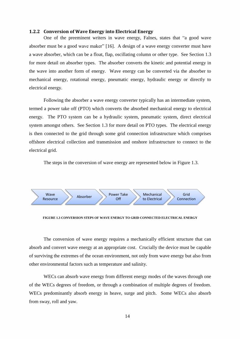
The steps in the conversion of wave energy are represented below in Figure 1.3.
FIGURE 1.3 CONVERSION STEPS OF WAVE ENERGY TO GRID CONNECTED ELECTRICAL ENERGY
The conversion of wave energy requires a mechanically efficient structure that can
absorb and convert wave energy at an appropriate cost. Crucially the device must be capable
of surviving the extremes of the ocean environment, not only from wave energy but also from
other environmental factors such as temperature and salinity.
WECs can absorb wave energy from different energy modes of the waves through one
of the WECs degrees of freedom, or through a combination of multiple degrees of freedom.
WECs predominantly absorb energy in heave, surge and pitch. Some WECs also absorb
from sway, roll and yaw.
Wave Resource
Absorber Power Take
Off Mechanical to Electrical
Grid Connection

15
1.3 Wave Energy Converters
Wave energy converters are designed to convert wave energy into other forms of
energy, normally electrical energy. In this section some broad categories of wave energy
converters are introduced with notable examples of each category presented.
The types of power take off (PTO) system typically found in these various categories
of WEC are also examined in this section. In Chapter 3 the type of generators for these PTOs
is discussed.
1.3.1 WEC Types
There are numerous divergent concepts for WEC devices and it would not be possible
to discuss these comprehensively here. WECs can be categorised in a variety of ways, the
most common being on the location of the WEC and the absorber type.
1.3.1.1 WEC Location:
WEC Locations can generally be categorised as onshore, nearshore and deep-water.
As outlined in previous sections this thesis focuses on deep-water WECs with electrical
transmission. However, some results and conclusions, particularly from Chapters 6 and 7,
will also be applicable to certain categories of onshore and nearshore WECs.
TABLE 1.5 DESCRIPTION AND EXAMPLES OF WECS BY LOCATION
Onshore
WEC
WECs are built into the shoreline or a
man-made breakwater and so are
accessible from land. This type of
WEC benefits from 24/7 accessibility
and close proximity to electrical
networks with the drawbacks of a
lower energy resource due to the
shallow water next to land, tidal range

16
issues, and also less scalability due to
terrestrial constraints. Onshore
devices are predominantly oscillating
water column type (see next section)
or a variant of a point absorber. Some
examples are shown opposite.
Top: WaveGen (Courtesy Peter
Church), Bottom: Wavestar (Courtesy
Sebastian Nils Swiatecki)
Nearshore
WEC
WECs are generally fixed structures
in depths less than 25m. These
structures are either piled to the
seabed or can be held in place with
gravity only. Thus this type of WEC
can take advantage of the increased
surge component in the wave at this
depth, more evenly spread
directionality, and also shorter
transmission distances (and the option
of hydraulic or pneumatic
transmission). Like onshore devices
the resource energy will be lower than
in deep-water and tidal ranges will be
an issue. Some examples are shown
opposite
Top: Aquamarine Oyster 800 (Courtesy
Aquamarine Power Ltd.), Bottom:
Oceanlinx Mk. II (Courtesy Oceanlinx)

17
Offshore
WEC
WECs are generally floating, moored
devices located in deep-water which,
for this thesis, is categorised as deeper
than 75m. This type of WEC can take
advantage of high energy resource
and also the possibility for very large
arrays due to large ocean areas. With
higher energy comes higher extremes
so survivability and accessibility for
this type of device will be
challenging. These devices will also
need extensive electrical systems for
collection and export of generated
power. Some examples are shown
opposite
Top: Pelamis P2 (Courtesy Pelamis
Wave Power Ltd.), Bottom: Wello
Penguin (Courtesy Wello Oy)
1.3.1.2 Absorber Type
WEC absorber types are relatively divergent and not all WECs can be put into a
specific category. Some of the main categories of WEC absorber are introduced in this
section.
Attenuators: Floating devices that are aligned perpendicular to the waves. These devices
capture energy from the relative motion of the two arms as the wave passes them
An example of an attenuator is the Pelamis device which has multiple sections which
articulate along the devices length. The articulated joints capture the wave energy in the
pitch and yaw modes. A hydraulic PTO is used within the device. At each joint hydraulic
cylinders provide damping force and convert the absorbed mechanical power to hydraulic
power. The hydraulic power can be smoothed via accumulators and converted to rotational
power via hydraulic motors. These in turn can be connected to electric generators.

18
Left: Attenuator Operating Concept (Courtesy Aquaret) and Right: Example (Courtesy
Pelamis Wave Power Ltd.)
Point Absorbers: Floating structures that can absorb energy from all directions. They covert
the motion of the buoyant top relative to the base into electrical power
An example of a point absorber is the Ocean Power Technologies (OPT) device which has
two bodies which have different natural responses to the wave resource. As a result of the
difference responses a relative linear motion between the bodies is induced by the wave
resource. A hydraulic PTO is used within the device to capture energy from the relative
motion. The hydraulic power can be smoothed via accumulators and converted to rotational
power via hydraulic motors. These in turn can be connected to electric generators.
Point Absorber Operating Concept and Example (Courtesy Ocean Power Technologies)

19
Submerged Pressure Differential: Devices capture energy from pressure change as the
wave moves over the top of the device causing it to rise and fall.
An example of a submerged pressure differential device is the Carnegie CETO device which
has a buoyant actuator connected to a hydraulic cylinder on the sea bed. The buoyant
actuator will react to the changing pressure differential as the wave resource passed over the
device. A hydraulic PTO is used within the device to capture energy from the buoyant
actuator. The hydraulic power can be transmitted to shore via high pressure pipelines and
converted to electrical power in a hydro-electrical plant.
Submerged Pressure Differential Operating Concept and Example (Courtesty Carnegie Wave
Energy Ltd.)
Oscillating Wave Surge Converters: Near-surface collectors, mounted on an arm which
pivots near the sea bed. The water particles in the waves cause the arm to oscillate and
generate power.
An example of an oscillating wave surge converter is the Aquamarine Oyster which has a
hinged buoyant flap, connected at the hinge to the sea bed. The buoyant flap reacts to the
passing wave resource and hydraulic cylinders connected to the flap capture the energy from
the resource. The hydraulic power can be transmitted to shore via high pressure pipelines and
converted to electrical power in a hydro-electrical plant. Alternatively an offshore oil-electric
PTO can be used to convert to electrical power allowing electrical transmission to shore.

20
Oscillating Wave Surge Converter Operating Concept and Example (Courtesy Aquamarine
Power Ltd.)
Oscillating Water Column (OWC) technologies convert the rise and fall of waves into
movements of air flowing past turbines to generate power.
An example of an oscillating water column is the Ocean Energy Buoy which is a floating
OWC. The Ocean Energy Buoy captures entrained air in an OWC chamber within the hull of
the device. This air is driven in and out of the chamber through a bi-directional air turbine.
The air turbine is coupled to a generator which generates electrical power for transmission to
shore.
Oscillating Water Column Operating Concept and Example (Courtesy Ocean Energy Ltd.)

21
Overtopping devices have a wall over which waves break into a storage reservoir which
creates a head of water. The water is released back to the sea through a turbine to generate
power.
An example of an overtopping device is the Wave Dragon which is a large buoyant structure
with a ramp facing the wave resource. The waves overtop, via the ramp, into a reservoir on
the structure. The reservoir is then drained, via low-head hydro-electric turbines, back to the
sea. The hydro-electric turbines are coupled to a generator which generates electrical power
for transmission to shore.
Overtopping Device Operating Concept and Example (Courtesy Erik Friis-Madsen)
Internal Rotating Mass Two forms of rotation are used to capture energy by the movement
of the device heaving and swaying in the waves. This motion may drive an eccentric weight
or a gyroscope causes precession. In both cases the movement is attached to an electric
generator inside the device.
An example of an internal rotating mass device is the Wello Penguin which is a large buoyant
structure shaped to induce motion in pitch and roll. A large concentric mass is located within
the hull of the device and the induced motion causes this mass to rotate. The concentric mass
is coupled to a low speed generator which generates electrical power for transmission to
shore.

22
Internal Rotating Mass Operating Concept and Example (Courtesy Wello Oy)
1.3.2 Wavebob
This thesis was undertaken with the support of Wavebob Ltd. The Wavebob device is
a point absorber type WEC which is under development. During the course of this research
the Wavebob device was used as a candidate device for some analysis. In particular the
expected generation characteristics and power output time series of the Wavebob device are
used in Chapters 4, 5 and 6. Although the Wavebob device was used as a candidate the
research is applicable to a wide variety of WEC concepts, in particular deep-water WEC
devices. Some of the research may be applicable also to other WEC concepts and potentially
for the tidal energy and floating offshore wind industries also.
Further details on the Wavebob device are given in Section 4.3.1.

23
2 Literature Review
Chapter 2
Literature Review
2.1 Introduction
A summary of the academic and industrial literature covering the main research
questions of this thesis is presented in this Chapter:
What electrical components are typical of, and what are the design requirements of, a
deep-water WEC array?
What is the techno-economic optimum electrical network design for WEC arrays?
What economic challenges and potential cost reductions exist for WEC array
electrical network designs?
How can resource induced flicker emissions, which are inherent to the wave energy
resource, be evaluated during the WEC design process and how can they be
mitigated?
What is the scale of the domestic Irish market for wave energy and the cost and
technical challenges of accessing export market opportunities?
Literature which focuses on these research questions and topics is presented and
critiqued in this Chapter. Any existing research which can be built on, or provides important
inputs to the research objectives of this thesis, is highlighted.
The topic of electrical networks and grid integration for WEC arrays has been
relatively underexplored in academia until now. There are several reasons for this. Firstly,
the main knowledge of this topic lies within WEC technology development companies and
the specific electrical systems are often seen as part of the company’s intellectual property.
This is problematic in itself as it prevents convergence of technology in the industry.
Secondly, the major concentration of the sector has been on prototyping single
demonstrator devices to date where the focus is not on economics of large scale commercial
installations. Also the electrical infrastructure usually belongs to a third party such as a test
site operator.

24
Thirdly, there is sometimes an assumption that the same offshore electrical networks
as offshore wind will be sufficient for WEC arrays. As will be demonstrated in this thesis,
while there is some relevant cross-over from offshore wind, there are important differences
which must be addressed.
To date the predominant focus of research around electrical systems has been in four
distinct areas namely;
Generators for WECs
Grid connection issues such as grid code compliance
Power Quality
Storage
The main objectives of this thesis relate to these areas and some elements from
literature are brought into the research and explored or critiqued. However, the volume of
literature in the analysis of electrical network design is comparatively small.
A comprehensive literature review ranging from early stage developments in wave
energy through to the most up to date publications has been undertaken to inform the original
research in this thesis. Some of the major publications, authors and themes are introduced,
evaluated, and critiqued in the subsequent sections.
2.2 Notable Publications
At the beginning of this research there was no authoritative publication in the area of
electrical systems for ocean energy. In 2013 a comprehensive book, “Electrical Design for
Ocean Wave and Tidal Energy Systems”, was published by the Institute of Engineering and
Technology (IET) [17]. The author of this thesis is a contributor to this book as shown in
Appendix A.
This book is an excellent reference for electrical design issues and brings together the
international research community in this area to provide a comprehensive text. Topics
covered within the book include; generators, cabling umbilical and array layout, power
system interaction, energy storage, control systems, modelling and simulation, and
economics.

25
The IET book is essentially a compilation of a range or researcher’s previous
publications. The most relevant sections to this thesis are Chapter 3, ‘Cabling umbilical and
array layout’ (P. Ricci and J.L. Media), and Chapter 5, ‘Grid integration: part 2 – power
quality issues’ (A. Blavette and J. MacEnri).
In Chapter 3 of the IET book Ricci et al present potential array layouts but do not
undertake a techno-economic analysis and, in fact, refer to the author of this thesis’ work as a
potential solution for techno-economic evaluation. There is also an evaluation of efficiency
for AC transmission schemes which has been conducted in a more comprehensive manner in
this thesis, see Chapter 4 of this thesis. Ricci et all present an evaluation of the ‘key
interfaces’ which are outlined in this thesis in Chapter 4. This evaluation, as will be
demonstrated in this thesis, makes several assumptions which devalue its contribution;
notably the requirement for subsea connection units (‘hubs’) and also the requirement for
fixed platform offshore substations. Ricci et al also conduct an analysis of the requirements
for dynamic cables which is a well researched piece of work.
In Chapter 5 of the IET book Blavette et al present a range of power quality
parameters and grid code requirements and evaluate their importance to wave and tidal
energy converters. This work is relatively high level and does not outline the relationship
between voltage flicker and WEC power output appropriately which has been
comprehensively presented in Chapter 6 of this thesis.
2.3 Generators for Wave Energy Converters
There has been a natural research focus on generators for wave energy converters due
to the current development stage of the industry. With wave energy converters there is a
variety of concepts for absorbing wave energy and a variety of concepts for converting the
absorbed energy to electrical energy as outlined in Chapter 1. Hence there is some interest in
generators for a variety of power take off (PTO) systems from hydraulics, air turbines, and
water turbines. Linear generators and low speed generators are also a topic of much interest
in wave energy due to their attraction in ‘direct drive’ conversion applications.
During the 1970s, the early days of wave energy system development, there was a
focus on generators at the University of Edinburgh as part of the Edinburgh Wave Energy
Project [18]. This project investigated generator types for the ‘Salter Duck’ type WEC.

26
Presently the leading research in the area of rotary generators for wave energy
converters is being undertaken by O’Sullivan [19], [20], [21] with a focus on generators for
OWC air turbines. Another prominent researcher in the area is Mueller who examines the
technical issues associated with selecting various types of rotary and linear generators [22]
and also focusses on generators for ‘direct drive’ WECs with a particular emphasis on linear
generators [23], [24]. Mueller also contributes to studies on the operation of generators with
seawater immersed windings [25].
With a predominant focus on linear generators, research undertaken at Uppsala
University focusses on the linear generator for the Seabased WEC. Leijon leads the work on
developing linear generator based WECs explaining the construction and testing of the linear
generator and associated equipment [26], [27], [28], [29]. Leijon is also a prominent
researcher of WEC electrical networks and submarine infrastructure, which is particularly
relevant to this thesis, as outlined in Section 2.6. There is also a large body of research from
Uppsala University on the subject of linear generator construction and testing [30], [31], [32].
The Uppsala/Seabased concept is unique to the wave energy industry and the output of this
group certainly represents the primary research in the area of linear generators for wave
energy.
Although generators for WECs is not a core research objective of this thesis some
generators for hydraulic PTO’s and direct drive PTO’s are discussed in Chapter 3 and the
topic relates somewhat to the overall design of electrical networks for WEC arrays. In
particular, the original research on voltage flicker presented in Chapter 6 is an important
addition to the knowledge base for PTO and generator selection. PTO design and generator
selection is currently undertaken without a accurate reference to voltage flicker impacts of the
selection. Therefore, while a PTO may be designed and a generator may be selected which
allow for highly efficient conversion of wave energy to electrical energy, this may introduce
power quality issues in the form of voltage flicker.
2.4 Grid Integration of Wave Energy
The topics of grid connection of WECs and WEC arrays, power quality, and energy
storage are interlinked and some researchers address a combination of these topics. In
general the focus of literature in these topics is around the effects wave plants will have on
the power system. These can be grid integration issues and grid code compliance or can be

27
more focussed on specific power quality issues, specifically steady state voltage control or
voltage flicker. In this section the major literature contributions, which have particular
relevance to this research, are discussed.
Santos [33], Boehme [34], Khan [35] and Ahmed [36] evaluate the capacity of the
grid infrastructure to allow large scale integration of ocean energy. Santos [33] presents a
case study of a number of WECs connected to the distribution system and evaluates the
steady state voltage effects at a variety of locations on the electrical network. Santos also
examines power losses and grid code compliance issues such as low voltage ride through.
Santos also presents the smoothing effect on the output power from aggregation effects which
are relevant to later discussions in Chapter 6. This work presents relevant studies which
would be conducted in a project development (for wind, wave, tidal etc.) so does not provide
any insight into the particularities of wave energy on voltage control.
Boehme [34] investigates load flow and constraint issues from the integration of large
scale wave and tidal energy in the Orkney Island electrical systems. An optimised load flow
is presented to maximise renewable energy resource while remaining within the thermal and
voltage limits of the existing power system. This again is a very specific study and provides
no insights into any particular impacts of wave energy on the electrical network.
Khan [35] undertakes a load flow analysis to determine the capacity of the Oregon
(U.S.A) electrical grid for wave energy, and to identify any potential bottlenecks in the
system and optimum points of connection to the system. Again this is a very specific study
and provides no insights into any particular impacts of wave energy on the electrical network.
Ahmed [36] investigates the effect of WEC arrays on the system voltage in the UK
with some analysis of fixed speed and variable speed generators for WECs. This paper
introduces the idea that voltage control will be particularly difficult for direct drive WECs but
the analysis is not very detailed into the real relationship between WEC resource and voltage
flicker emissions.
O’Sullivan [19] examines some of the challenges to the grid integration of WEC
arrays. This paper focuses on areas such as connection charging regimes, use of system
charges, grid code compliance and presents a costed case study 20MW wave farm. This
paper is a useful overview of some of the regulatory issues associated with grid connection
and how they may affect wave energy economics. Blavette and O’Sullivan [37] examine grid

28
compliance issues in more detail and present some control strategies for WECs to ensure
compliance. Blavette and O’Sullivan also [38] undertake a case study of grid connected
WEC arrays in Ireland with a focus on load flow, steady state voltage limits and grid code
compliance. While this work is somewhat relevant to particular project assessment it is
routine analysis for connection of renewable generation and does not particularly advance the
knowledge of WEC array grid integration.
2.5 Power Quality and Energy Storage
The topic of power quality has perhaps the largest volume of literature in the research
area of electrical systems for wave energy. The focus is mainly on voltage quality issues
caused by the connection of wave energy converters to the electrical grid and areas such as
voltage regulation, flicker, and mitigation effects are investigated. One of the solutions to
flicker is energy storage which is evaluated by a number of researchers.
Nambiar and Kiprakis et al investigate voltage effects, array configurations effects
and other mitigation approaches to power quality [39], [40], [41], [42]. In these papers
Nambiar presents a ‘wave-to-wire’ model which can simulate the power output of a WEC or
WEC array with a variety of spatial configuration options. Nambiar evaluates physical
spatial aggregation effects from WEC arrays and the mitigation effects this will have on the
voltage at the point of connection. Nambiar focusses on the steady state voltage effects and
does not address flicker directly. The spatial model that is presented gives physical
aggregation effects only and does not consider hydrodynamic interference effects. This
research is a useful basis for further assessment but primarily focuses on the control strategies
for steady state voltage.
Blavette and O’Sullivan have completed studies around power quality also in areas
such as flicker and voltage regulation. Blavette et al [43] present the potential flicker output
from a number of OWC type WECs. These WECs exhibit constantly varying power output
at twice the resource frequency (as the air flows through the turbine twice per wave period)
and due to this cause flicker issues at the point of connection. This was the first publication
which correctly linked voltage flicker and wave resource and was followed by a paper from
the author of this thesis with similar conclusions. This paper outlines the potential issue with
flicker from ‘direct drive’ WECs and shows that the smoothing expected from other RES
sources such as wind turbines may not be seen with WEC arrays.

29
Blavette [44] also presents a dynamic model for assessment of power quality of both
wave and tidal energy converters and highlights some inadequacies in grid codes for ocean
energy devices.
The issue of energy storage to mitigate power fluctuations and hence flicker from a
wave energy plant is investigated also by Murray [45] and Muthukumar [46], [47] which
suggest various energy storage techniques to smooth the output from wave energy arrays to
the electrical grid. Murray investigates the use of supercapacitors as a storage medium
concluding that lifespan may be an issue. Muthukamar investigates the addition of inertia
energy storage to an OWC type WEC concluding that this has a smoothing effect on power
fluctuations. Neither researcher consider at the lifetime costs of the storage devices, nor at
their impact on overall efficiency.
Blavette and O’Sullivan also present a generic study of storage for mitigation of
flicker emissions [48].
Although power quality and flicker have been extensively covered to date it is
concluded that the issue has not been simplified sufficiently to feed into the plans of WEC
designers. This issue of ‘resource induced’ flicker has not been explored in as detailed a
manner and the sea-states that are likely to cause the greatest flicker issues have not been
analysed. A more comprehensive understanding of the voltage flicker issues with WECs
would be an extremely valuable addition to the knowledge base.
Therefore, power quality, specifically resource induced flicker, has been included as a
research objective in this thesis. The intention is to develop practical, understandable tools
for WEC designers to assist in understanding and characterise the flicker issue further. This
research is presented in Chapter 6 of this thesis.
2.6 WEC Array Electrical Networks
A central research objective for this thesis is the techno-economic analysis of WEC
array electrical networks. There is little research on this topic; a gap exists which is
addressed in this thesis.
As with electrical generators for WECs, earlier work on WEC array electrical
networks was undertaken as part of the Edinburgh Wave Energy Project in the 1970s. This

30
work investigated the electrical networks for connecting multiple ‘Salter Ducks’ together in a
‘spine’ and exporting the power to shore [49], [50]. This work is extremely interesting but
there have been huge advances in electrical infrastructure since the 1970s and offshore wind
has pioneered the way in this regard as shown in Chapter 3. The drivers of this research,
however, are similar; focussing on cost effective electrical network designs.
Ricci has produced and contributed to a number of important papers around electrical
networks for WEC arrays. In [51] both HVAC and HVDC export schemes are assessed for
large WEC arrays. The cost and efficiency of these schemes are evaluated and presented.
Costs for three WEC array electrical networks are calculated (9.75MW, 19.5MW and
48.75MW). Although this is a useful study, no comparison of array configurations is
undertaken and the key interface components are not considered. Offshore substations are
also required which may present a design challenge for WEC arrays, particularly in deep-
water, as outlined in this thesis (see Chapters 4 and 5). In [52] electrical network
configuration is introduced as an important factor in the spatial configuration of WEC arrays.
Ricci also published one of the more practical analyses of wave energy electrical systems,
particularly at the interface level [53]. This looks at a variety of concepts for connecting the
devices to the electrical network and is a useful and insightful publication. The major
drawback of this work is that it only considers submarine/floating ‘hubs’ as integration and
does not consider the practical or economic aspects of using same. In this thesis a strong case
is built that submarine ‘hubs’ should not be necessary for WEC array electrical networks.
Ricci also contributed to a study on the dynamic performance of a WEC dynamic cable
which is of interest, but not central, to this work [54]
Lopez et al present a review of potential WEC array electrical networks with a focus
on transmission technology [55]. This gives a comparison of various HVAC and HVDC
transmission systems. The array electrical network is assumed to mirror that of an offshore
wind farm with some potential solutions proposed within these constraints.
Igic et al examined the potential WEC array electrical network for the Wavedragon
WEC [56]. The focus in this study was the possibility of combining the inverter side of the
generator power converter into a single unit, i.e. individual WECs would connect together on
the DC bus. Similar research has also been conducted for offshore wind but DC aggregation
systems have not been shown to be cost effective.

31
Kenny [57] developed multiple connection schemes for wave energy and endeavoured
to build a cost model to compare the various options. This work was a very good baseline for
some of the material analysed in this thesis but the methodology was not comprehensive. A
review of available technologies was undertaken and these technologies were ‘bolted’
together to develop electrical configurations. No critical analysis was undertaken as to
whether these technologies were appropriate in the first instance.
Through Uppsala University and Seabased, Leijon also focussed on wave energy
electrical networks for wave farms [58], [59], [60]. The focus of this research is on the linear
generator based technology which is at the kW rating and is not wholly applicable to large
scale arrays. The focus of the Uppsala research is also on submarine substations and power
conversion equipment. The viability of this approach is evaluated further within the work
and a strong case made against it.
Outside of academic literature there are some important reports which are relevant to
this thesis. The Equimar project is an EU FP7 project which ran from 2008 to 2011 exploring
performance, cost and environmental impact of marine energy devices. Deliverable 5.1 was
“Guidance Protocols on Choosing of Electrical Connection Configurations” [61]. This
deliverable gave a high level view of the issues surrounding the grid integration of marine
energy such as grid codes, test site infrastructure, elements of the electrical system, and some
possible AC and DC connection configurations. The Equimar work lacked some practical
application and did not comprehensively compare the various network configurations.
WaveNet [62] also investigated electrical networks but at an early stage in the industry. The
current DTOcean project is exploring techno-economics of electrical network configurations
in detail but is incomplete at this time.
Finally, there are a number of test centres operational around Europe which offer grid
connected ‘berths’ for testing wave and tidal technologies. The most developed of these is
the European Marine Energy Centre (EMEC) in Orkney, Scotland. The practical experience
in electrical network installation from these test centres is presented in Chapter 3 and
referenced throughout the thesis as these locations are the only real deployment of electrical
networks to date in the wave energy industry.
From a thorough review of the research literature for electrical networks for WEC
arrays it is evident that significant gaps exist. Therefore a comprehensive research thesis on

32
this topic was identified as extremely valuable to the industry and research community.
Hence, WEC array electrical networks are the primary focus of the research in this thesis.
2.7 Offshore Wind Electrical Networks & Economics
As a much more mature industry, there is a vast amount of literature available which
has analysed the electrical network configurations for offshore wind farms. This provides an
excellent baseline for the research into electrical networks for WEC arrays, and the body of
research is generally more practical and based on real applications and experience. Below is
an outline of some useful sources from the large body of available literature.
The state of the art thinking has been summarised in books by Ackermann [63] and
Twiddell [64]. From these books it is clear that there has been significant convergence in the
design of electrical networks for offshore wind and the industry has moved towards 33kV
radial array networks with HVAC export transmission from offshore substations with a more
recent move to HVDC export transmission. This has proved the least costly option with all
of the required functionality. However, there are characteristics of wave energy which will
mean that offshore wind farm electrical systems cannot simply be replicated. Nevertheless,
the rationale behind this convergence was used as a guide for wave energy electrical
networks.
Although electrical network configuration has converged there are still alternative and
new ideas presented in the literature. In [65] some alternative array electrical network
configurations for offshore wind are evaluated showing potential benefits from non-radial
configurations and additional sectionalising of the electrical protection system, albeit with
additional cost. Switching overvoltages, earthing and reliability of various configurations are
also evaluated. In [66] HVAC and HVDC configurations are evaluated for the connection of
offshore renewables to the grid and an excellent overview of cables and offshore substations
is given including some costs. In [67] the cost and performance of the collection and export
system for offshore wind farms is examined.
[68], [69], [70], and [71] are excellent review papers covering electrical network
redundancy, reliability, losses, and capacity factors for offshore wind.
In the analysis conducted throughout this thesis offshore wind is used as a baseline
reference in each case. In particular, the economics of offshore wind served as a useful

33
guideline for economic modelling. Further details on the cross-over areas from offshore wind
to WEC arrays are given in Chapter 3.
2.8 Array Layout
The spatial layout of WEC arrays is an important factor in understanding the
requirements for the electrical network techno-economic analysis. The layout of arrays is a
complex topic requiring knowledge of hydrodynamics, wave resource, mooring systems, and
control systems amongst others. To develop a full understanding of all these areas would be
outside the scope of this research. However some of the relevant literature was reviewed to
endeavour to characterise the issue.
C. Fitzgerald [72] outlines the hydrodynamic separation requirements for optimum
performance of a WEC array. J. Fitzgerald [73] and [74] assesses the mooring requirements
for WEC separation and also evaluates the array spacing for WEC arrays.
Child [75], Ricci [76], and Cruz [77] present array spatial configurations analyses
which provide some guidance as to WEC separation requirements. Westphalen [78]
demonstrates how the control of WECs within an array can also influence the required spatial
configuration. In Chapter 4 the analysis of spatial configuration requirements is used to
inform the design of an optimum WEC array electrical network.
2.9 Dynamic Rating
Another research objective in this thesis was to apply the emerging technologies in
the dynamic or real time ratings area to WEC array electrical networks as a means of
improving the economics of these networks. The area of dynamic ratings is predominantly
used in the transmission and distribution industry and this was where the literature was
concentrated. Some case studies and analysis using dynamic and real time ratings for
transmission systems are given in [79], [80], [81], and [82].

34
2.10 Literature Review Summary
From a comprehensive review of the literature it is evident that much of the research
in electrical systems for wave energy has been concentrated on the generator and grid
connection level including a focus on power quality. There is a lack of in-depth research
undertaken on the practical implementation of electrical networks for wave energy arrays.
Prominent researchers in this areas are Ricci and Leijon. Ricci’s work has been of particular
interest in this thesis, and is built upon and improved. Leijon’s work is very focussed on the
Seabased technology concept and is not as relevant to generic offshore WECs.
There are also gaps in the existing research on power quality issues, particularly
voltage flicker. Blavette in particular has advanced the research in this topic significantly.
However, particular value to the knowledge base can be added by better characterising
voltage flicker in relation to WEC power output, and by providing practical tools for
assessing voltage flicker at the design stage,
Therefore, the main objectives of this thesis have gaps in the knowledge base and
provide significant scope for novel and original research. This practical, industrial, thesis is
aimed at filling these knowledge gaps and will be a valuable addition to the industry’s
knowledge base. At the present time the industry is developing from prototype testing
towards commercial projects. This thesis, its results, and conclusions will be timely in this
regard.
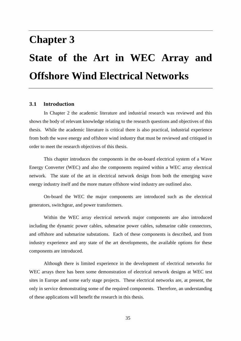
35
3 State of the Art in WEC Array and Offshore Wind Electrical Networks
Chapter 3
State of the Art in WEC Array and
Offshore Wind Electrical Networks
3.1 Introduction
In Chapter 2 the academic literature and industrial research was reviewed and this
shows the body of relevant knowledge relating to the research questions and objectives of this
thesis. While the academic literature is critical there is also practical, industrial experience
from both the wave energy and offshore wind industry that must be reviewed and critiqued in
order to meet the research objectives of this thesis.
This chapter introduces the components in the on-board electrical system of a Wave
Energy Converter (WEC) and also the components required within a WEC array electrical
network. The state of the art in electrical network design from both the emerging wave
energy industry itself and the more mature offshore wind industry are outlined also.
On-board the WEC the major components are introduced such as the electrical
generators, switchgear, and power transformers.
Within the WEC array electrical network major components are also introduced
including the dynamic power cables, submarine power cables, submarine cable connectors,
and offshore and submarine substations. Each of these components is described, and from
industry experience and any state of the art developments, the available options for these
components are introduced.
Although there is limited experience in the development of electrical networks for
WEC arrays there has been some demonstration of electrical network designs at WEC test
sites in Europe and some early stage projects. These electrical networks are, at present, the
only in service demonstrating some of the required components. Therefore, an understanding
of these applications will benefit the research in this thesis.

36
In the offshore wind industry there is vast experience of design of electrical networks
which have converged allowing specific installation vessels, installation procedures and
interface designs to be used for any large offshore wind farm. With larger offshore wind
farms being developed further from shore there is a move to HVDC export systems to allow
for the large power and long transmission distances. The wave energy industry can learn
from the offshore wind industry in order to achieve early convergence in the design of WEC
array electrical networks and, as a consequence, cost reduction.
3.2 WEC On-Board Electrical Systems
Within the wave energy converter device itself electrical components are required to
convert mechanical power to electrical power, condition the generated power to grid
compliant requirements, step up the voltage for export, provide auxiliary supplies, isolation
for maintenance, and electrical protection from faults.
3.2.1 Generators
An electrical generator is required to convert captured mechanical power into
electrical power. The selection of a generator for a WEC depends on the type of power take
off (PTO) system. Environmental factors and grid code compliance must also be considered.
For example in the case of a hydraulic PTO the generator would be coupled to a rotating
hydraulic motor. In the case of a direct drive PTO this could be a linear generator or rotary
generator coupled via a mechanical linear to rotary conversion system such as a rack and
pinion.
3.2.1.1 Generator Types
There are numerous types of electrical generator which are used in various WEC
designs. Within the power system all large thermal and hydroelectric power plants use
synchronous generators and these have certain characteristics that support the operation of
large electrical power systems. The majority of wind turbines use double fed induction
generators to allow for variable speed operation but there is a move to direct drive generators,
particularly offshore, to allow for the removal of the gearbox from the wind turbine, which
can be a major source of failures and maintenance. Even within the different types of

37
generator there are different subtypes and even still variations on the subtypes, mostly in
construction or flux linkage type.
The selection of a generator for a WEC is a complex task. Some of the main types
and subtypes of generator are given in Table 3.1. Some more details on these various types
of generators can be found in [63].
TABLE 3.1 MAJOR TYPES AND SUBTYPES OF ELECTRICAL GENERATORS FOR WAVE ENERGY
Generator Type Generator Subtype
Synchronous Field Wound with Static Excitation
Field Wound with Brushless Excitation
Field Wound with PMG Excitation
Permanent Magnet Field
Asynchronous Squirrel Cage Induction
Wound Rotor Induction
Double Fed Induction
Permanent Magnet Generators See Synchronous – Permanent magnet
field Switched Reluctance Generators
DC Generators
High Voltage Generator (Powerformer)
Table 3.1 applies to rotary machines but can also apply to linear generators with
permanent magnet and switched reluctance being two relatively common types of linear
generator in the literature.
In the following section the type of generator for several distinct PTO cases are
discussed briefly. This gives a cross section of the type of generator which would be required
for a given PTO at various stages of development.
3.2.1.2 Directly Connected SCIG with Hydraulic PTO
The choice of generator for a prototype WEC with a hydraulic PTO, and all pre-
commercial, one-off hydraulic PTO prototypes would be a fixed speed squirrel cage
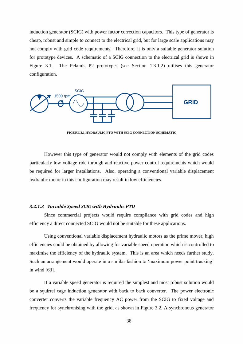
38
induction generator (SCIG) with power factor correction capacitors. This type of generator is
cheap, robust and simple to connect to the electrical grid, but for large scale applications may
not comply with grid code requirements. Therefore, it is only a suitable generator solution
for prototype devices. A schematic of a SCIG connection to the electrical grid is shown in
Figure 3.1. The Pelamis P2 prototypes (see Section 1.3.1.2) utilises this generator
configuration.
FIGURE 3.1 HYDRAULIC PTO WITH SCIG CONNECTION SCHEMATIC
However this type of generator would not comply with elements of the grid codes
particularly low voltage ride through and reactive power control requirements which would
be required for larger installations. Also, operating a conventional variable displacement
hydraulic motor in this configuration may result in low efficiencies.
3.2.1.3 Variable Speed SCIG with Hydraulic PTO
Since commercial projects would require compliance with grid codes and high
efficiency a direct connected SCIG would not be suitable for these applications.
Using conventional variable displacement hydraulic motors as the prime mover, high
efficiencies could be obtained by allowing for variable speed operation which is controlled to
maximise the efficiency of the hydraulic system. This is an area which needs further study.
Such an arrangement would operate in a similar fashion to ‘maximum power point tracking’
in wind [63].
If a variable speed generator is required the simplest and most robust solution would
be a squirrel cage induction generator with back to back converter. The power electronic
converter converts the variable frequency AC power from the SCIG to fixed voltage and
frequency for synchronising with the grid, as shown in Figure 3.2. A synchronous generator
1500 rpm
GRID
SCIG

39
could also be used here giving some benefits (such as a simpler rectifier); however the SCIG
is considered simpler than a synchronous generator, i.e. no excitation or brushgear
requirements. The Aquamarine Oyster (see Section 1.3.1.1) onshore hydroelectric plant uses
this generator configuration, albeit with a water hydraulic Pelton wheel turbine.
FIGURE 3.2 HYDRAULIC PTO WITH SCIG AND POWER CONVERTER CONNECTION SCHEMATIC
However, the use of axial piston type digital displacement (DD) hydraulic motors
such as those developed by Artemis Intelligent Power [83] could achieve high efficiencies in
the hydraulic system at fixed speed and use conventional synchronous generators, as shown
in Figure 3.3. Brushless synchronous generators may be more suitable to the marine
environment. This would comply with the requirements of the grid codes and also remove
the need for a power electronics converter for interfacing with the grid.
FIGURE 3.3 DIGITAL DISPLACEMENT HYDRAULIC PTO WITH SYNCHRONOUS GENERATOR CONNECTION
SCHEMATIC
In the case of variable and fixed-speed, other generator options could be explored but
would not give any major benefits over those selected here. No current working WEC
prototypes use this configuration.
1000-
1600 rpm
GRID
SCIG
Power Converter
1500 rpm
GRID
Synch Gen DD Motor

40
3.2.1.4 Linear Direct Drive PTO
Another type of direct drive PTO which has been considered for many WEC concepts
is a linear direct drive PTO. This PTO uses a linear generator to convert the linear motion
directly to electrical power.
Linear generators operate under the same principle of rotary generators, only instead
of the electromagnetic flux being cut by an angular rotation motion it is cut by a linear
motion. Essentially the linear generator is a section of rotary generator with a very large
radius or a rotary generator rolled out flat.
Linear generators have long been of interest to the ocean energy community with a
number of pilot projects and seagoing devices already tested. In particular they lend
themselves very well to point absorber type WECs as the linear reciprocal motion can be
converted to electrical power.
As with rotary generators there are various types of linear generators. The most
developed are permanent magnet linear generators and switched reluctance linear generators.
Again there are a variety of subtypes of each of these generators with a particular emphasis
on the construction of the stator and translator of the generator
There are a number of potential benefits of using a linear generator such as having
less mechanical parts (within the overall WEC) and high wave to wire efficiency. However,
there are also several drawbacks as the technology is relatively immature, the machines can
be extremely large due to low speed operation (in comparison to a rotary equivalent) and
there are mechanical challenges in bearings and linear guidance systems. Issues with power
quality also exist with this concept as detailed in Chapter 6.
A linear generator requires a power electronic converter interface with the grid. This
allows the variable frequency, variable voltage output from the linear generator to be
converted to a fixed frequency, fixed voltage output to the electrical grid. Figure 3.4 shows a
typical connection schematic for a linear generator PTO WEC. The Seabased WEC concept
(see Figure 3.16) uses this generator configuration.
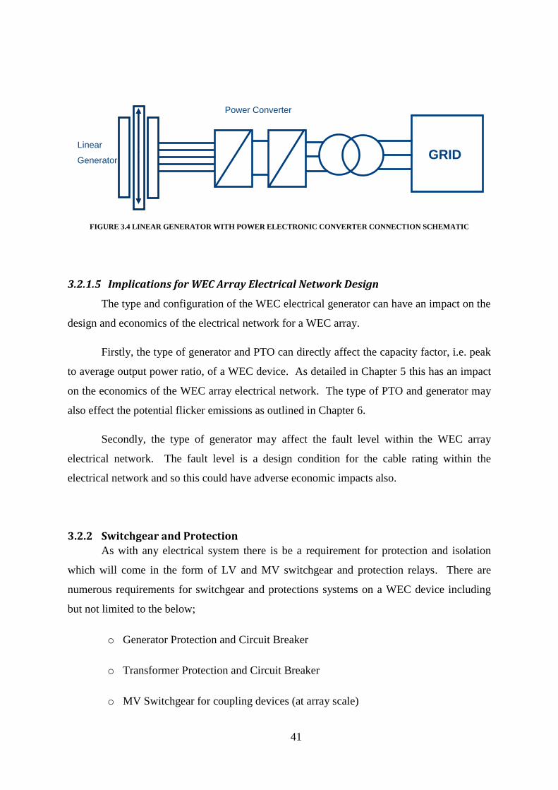
41
FIGURE 3.4 LINEAR GENERATOR WITH POWER ELECTRONIC CONVERTER CONNECTION SCHEMATIC
3.2.1.5 Implications for WEC Array Electrical Network Design
The type and configuration of the WEC electrical generator can have an impact on the
design and economics of the electrical network for a WEC array.
Firstly, the type of generator and PTO can directly affect the capacity factor, i.e. peak
to average output power ratio, of a WEC device. As detailed in Chapter 5 this has an impact
on the economics of the WEC array electrical network. The type of PTO and generator may
also effect the potential flicker emissions as outlined in Chapter 6.
Secondly, the type of generator may affect the fault level within the WEC array
electrical network. The fault level is a design condition for the cable rating within the
electrical network and so this could have adverse economic impacts also.
3.2.2 Switchgear and Protection
As with any electrical system there is be a requirement for protection and isolation
which will come in the form of LV and MV switchgear and protection relays. There are
numerous requirements for switchgear and protections systems on a WEC device including
but not limited to the below;
o Generator Protection and Circuit Breaker
o Transformer Protection and Circuit Breaker
o MV Switchgear for coupling devices (at array scale)
GRID
Linear
Generator
Power Converter

42
o Auxiliary Switchgear
o Consumer Units (MCBs)
o DC Consumer Units (MCBs)
The auxiliary switchgear and consumer units are simple equipment used in standard
industrial applications and require no further mention here.
The generator protection is likely to be low voltage (LV <1000V) due to the size of
the generators. Medium voltage switchgear shall be required to connect multiple devices
together in an array.
3.2.2.1 Implications for WEC Array Electrical Network Design
The MV switchgear within a WEC array electrical network allows for isolation for
installation, maintenance, or post faults. The MV switchgear will also operate in the event of
a fault. These are crucial functions to the operation of the WEC array and the MV switchgear
is identified as a ‘key interface’ and explored in detail in Chapter 4. Whereas in offshore
wind the MV switchgear is always located in the wind turbine itself there may be a rationale
for separating this from the WEC within WEC arrays. However, separating the MV
switchgear from the WEC device may also present challenges both economically and
technically. In Chapter 4 this is analysed in detail.
3.2.3 Transformers
Because of the present power rating of WECs it is likely that they will generate at low
voltage (LV) within the WEC itself. However in order to export the generated power to the
electrical system the voltage level will have to be stepped up via a transformer to medium
voltage (MV). This facilitates both the transmission from the WEC to shore and also the
connection to the local electrical grid. A transformer is therefore required to step up the
voltage from LV to MV.

43
3.2.3.1 Transformer Types
The subject of power transformers is a comprehensive topic but in general
transformers can be classified in a number of ways:
o Insulation Medium
o Cooling Method
o Vector Group
Due to the environment within which the WEC is located, the critical issue for
transformer selection for WEC devices is the insulation medium. There are three main
insulation mediums for power transformers, shown in Figure 3.5:
o Dry Type (E.g. Cast Resin or Open Wound (‘dip and bake’))
o Oil Filled
o Synthetic Fluid Filled
FIGURE 3.5 LEFT TO RIGHT: DRY TYPE, OIL FILLED AND SYNTHETIC FLUID FILLED (COURTESY PELAMIS WAVE
POWER LTD.) TRANSFORMERS
3.2.3.2 On-board Transformers
The main requirement for an on-board transformer would be to step the voltage up for
transmission. The voltage would be stepped up from LV to MV. Typical MV voltage levels
(sometimes country specific) are 10kV, 11kV, 20kV, 33kV & 38kV. Typical LV generator
voltage levels are 400V, 415V, 480V and 690V. The choice of voltage is dependant on
equipment ratings and the overall design of the WEC array electrical network.

44
Another function of the transformer would be to step the voltage up or down for
supply of on-board auxiliary loads. This would be a low power transformer (10’s of kW) so
would be considered a relatively minor piece of plant.
Oil filled transformers would most likely be unsuitable due to the environmental risks
of an oil spill or potential fire risks. More likely are Dry Type and Synthetic Fluid Filled.
Dry type transformers use a solid dielectric such as cast resin as insulation around the
core and windings. Therefore heat losses are dissipated directly to the air meaning a large
surface area is required. These transformers are simple and robust; however they usually
require an additional housing as power parts are generally exposed. As the transformer is air
cooled it is possible that this housing will require air conditioning of some type which could
mean that the transformer is exposed to the saline atmosphere. This type of transformer is
simple and robust but the additional requirements may make it challenging for installing
within the WEC itself. There is considerable experience in the use of dry type transformers
in the marine industry.
Synthetic Fluid Filled transformers are especially useful where there is an
environmental or fire concern such as within a building, train tunnel or on an offshore
platform. The silicon based synthetic fluid is used as the dielectric and cooling medium so a
tank is also required and therefore they appear identical to an oil filled transformer. The
synthetic fluid would have a high fire point (>300°C), high moisture tolerance, and be
environmentally biodegradable. Midel 7131 is an example of this fluid (www.midel.com). A
synthetic fluid filled transformer is used in the Pelamis device. It has the advantages of an oil
filled transformer in that it is self contained (no housing required) and could be water cooled
to avoid air ingress into the dry compartments.
3.2.3.3 Implications for WEC Array Electrical Network Design
The transformers within a WEC array electrical network shall increase the voltage to
a suitable level for export. Whereas in offshore wind the transformer is always located in
each wind turbine itself there may be a rational for separating this from the WEC within
WEC arrays. However, separating the transformer from the WEC device may also present
challenges both economically and technically. In Chapter 4 this is analysed in detail.
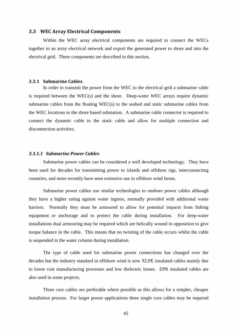
45
3.3 WEC Array Electrical Components
Within the WEC array electrical components are required to connect the WECs
together in an array electrical network and export the generated power to shore and into the
electrical grid. These components are described in this section.
3.3.1 Submarine Cables
In order to transmit the power from the WEC to the electrical grid a submarine cable
is required between the WEC(s) and the shore. Deep-water WEC arrays require dynamic
submarine cables from the floating WEC(s) to the seabed and static submarine cables from
the WEC locations to the shore based substation. A submarine cable connector is required to
connect the dynamic cable to the static cable and allow for multiple connection and
disconnection activities.
3.3.1.1 Submarine Power Cables
Submarine power cables can be considered a well developed technology. They have
been used for decades for transmitting power to islands and offshore rigs, interconnecting
countries, and more recently have seen extensive use in offshore wind farms.
Submarine power cables use similar technologies to onshore power cables although
they have a higher rating against water ingress, normally provided with additional water
barriers. Normally they must be armoured to allow for potential impacts from fishing
equipment or anchorage and to protect the cable during installation. For deep-water
installations dual armouring may be required which are helically wound in opposition to give
torque balance in the cable. This means that no twisting of the cable occurs whilst the cable
is suspended in the water column during installation.
The type of cable used for submarine power connections has changed over the
decades but the industry standard in offshore wind is now XLPE insulated cables mainly due
to lower cost manufacturing processes and low dielectric losses. EPR insulated cables are
also used in some projects.
Three core cables are preferable where possible as this allows for a simpler, cheaper
installation process. For larger power applications three single core cables may be required

46
due to the required current carrying capacity. Three single cores also allows for cheaper
redundancy as a fourth single core cable can be installed as a redundant phase where a second
full three core cable is required for redundancy in a three core application.
A fibre optic cable can be installed within the submarine power cable to allow for
communications. Figure 3.6 shows the typical construction of a medium voltage XLPE
submarine power cable. The fibre optic cable is not shown but would be installed within the
filler (8)
FIGURE 3.6 TYPICAL THREE CORE MEDIUM VOLTAGE SUBMARINE CABLE [84]
3.3.1.2 Dynamic Power Cables
Dynamic Cables (sometimes referred to as risers or umbilicals) are a specialised type
of submarine power cable that connect the electrical system on the floating WEC to the static
cable on the seabed. The dynamic cable is designed for the rigorous duty of being suspended
in the water column and undergoing the cyclic forces which are induced by the movement of
the WEC.
As shown in Figure 3.7 the dynamic cable configuration can vary. The free hanging
catenary is the simplest configuration but there will be loading on the full cable and scour
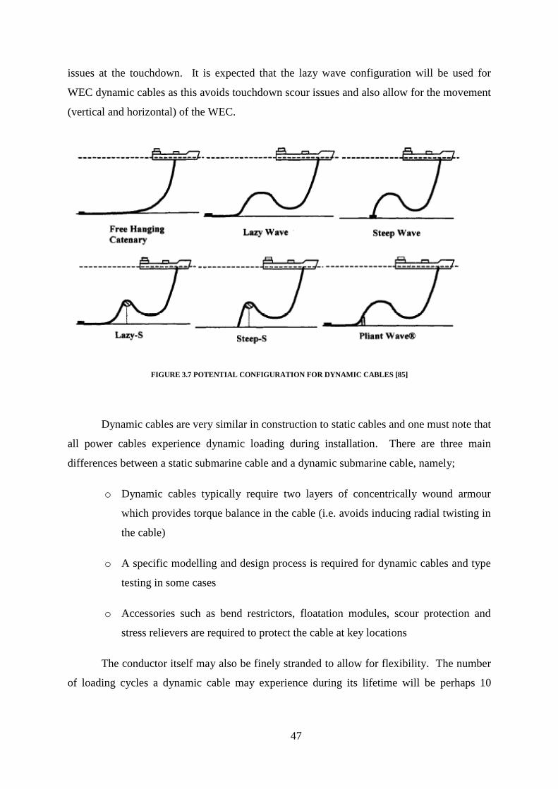
47
issues at the touchdown. It is expected that the lazy wave configuration will be used for
WEC dynamic cables as this avoids touchdown scour issues and also allow for the movement
(vertical and horizontal) of the WEC.
FIGURE 3.7 POTENTIAL CONFIGURATION FOR DYNAMIC CABLES [85]
Dynamic cables are very similar in construction to static cables and one must note that
all power cables experience dynamic loading during installation. There are three main
differences between a static submarine cable and a dynamic submarine cable, namely;
o Dynamic cables typically require two layers of concentrically wound armour
which provides torque balance in the cable (i.e. avoids inducing radial twisting in
the cable)
o A specific modelling and design process is required for dynamic cables and type
testing in some cases
o Accessories such as bend restrictors, floatation modules, scour protection and
stress relievers are required to protect the cable at key locations
The conductor itself may also be finely stranded to allow for flexibility. The number
of loading cycles a dynamic cable may experience during its lifetime will be perhaps 10

48
million or more. Specialist companies, such as JDR Cables, have expressed confidence in
their analysis tools to allow the cable survive the rigorous duty expected.
Figure 3.8 shows a cross section of a 3.3kV, 6 x 60mm2 cable which was developed
by JDR Cables for the OPT Powerbuoy. This shows the dual armouring, finely stranded
copper conductors (and two conductors per phase) and fibre optic cables in the central filler.
The insulation material chosen is ethylene propylene diene monomer (EPDM) rubber in this
case which has good flexibility properties.
FIGURE 3.8 DYNAMIC CABLE CROSS SECTION (COURTESY JDR CABLES)
3.3.1.3 Cable Installation and Connection
Methods for cable installation and post protection are well established in offshore
wind and outlined in Section 3.6. In general WEC arrays will be able to use the same
methods. However, there are some different installation requirements and risks for WEC
arrays which should be noted.

49
Firstly, offshore WEC arrays are likely to be in deep-water, at least 75m depth.
Presently, as outlined in Section 3.6 most offshore wind farms are located in depths of 10-
30m. This presents an additional challenge for installation particularly where any diving
activities are required.
Secondly, the weather risk associated with installation contracts for WEC arrays will
be large. In general offshore wind farm sites have been selected to be in relatively benign
sites to reduce the weather risk. WEC array sites will be in high energy areas such as the
western European seaboard. This is necessary for energy yield from the WEC arrays but is a
challenge to the installation of submarine cables.
Thirdly, offshore WECs are floating structures, unlike wind turbines. This means that
a dynamic cable is required to allow cable connection while the WEC moves freely to absorb
energy. The devices must be connected to these dynamic cables, most likely at the site itself.
The dynamic cables also have to be connected to the static submarine cable (see next
section). These areas have also been identified as ‘key interfaces’ and are explored in detail
in Chapter 4.
3.3.2 Submarine Connectors
The dynamic cable is a specialised cable and so is only used for the connection
between the WEC and the seabed where the dynamic cable is connected to a static submarine
cable. Therefore a connection needs to be made between the two types of cable. There is
also a possibility that a cable may be required to connect to a submarine component such as a
hub or substation. There are a variety of submarine cable connection options but they
broadly fall into four categories
1. Splice Connection (Figure 3.9) – A permanent splice/joint is made to join the
dynamic cable to the static cable. This could be done during cable manufacture. If
the cable is to be separated again it would require the joint being physically cut.

50
FIGURE 3.9 SUBMARINE POWER CABLE JOINT ASSEMBLY (COURTESY WARDOPERATIONS.COM.AU)
2. Splice Housing (Figure 3.10) – A splice is made in a prefabricated housing. In this
case the two ends of the dynamic and static cable would be lifted onto a work vessel
and the splice made over a number of hours. The connection is then lowered onto
the seabed. The splice can be undone and the cable capped with a similar
procedure.
FIGURE 3.10 J&S LTD. SPLICE HOUSING (COURTESY J&S LTD)
3. Dry-Mate Connection (Figure 3.11) – A connector is prefabricated in two parts and
the dynamic and static cables are spliced into either part during fabrication or on
site. Once the two parts of the dry-mate connector are spliced they can both be
lifted onto a work vessel and the connection made in a number of hours. The
connection can then be lowered onto the seabed. The connection can be lifted and
opened / closed numerous times without any further cable jointing work required

51
FIGURE 3.11 DRY MATE CABLE CONNECTORS. LEFT (COURTESY HYDROGROUP), RIGHT (COURTESY
MACARTNEY)
4. Wet-Mate Connection (Figure 3.12) – Like the dry mate connector this is a re-
usable connector, however it is located on the seabed. The connection can be
opened / closed numerous times on the seabed, however most likely requires the use
of a dynamic positioning class vessel.
FIGURE 3.12 MACARTNEY 11KV WET-MATE CABLE CONNECTOR (COURTESY MACARTNEY)
The connectors are generally expected to be more expensive and require more
expensive installation processes going from 1-4 above. Most of the connectors have been
developed up to 10-11kV, with some already available up to 36kV.
Connectors can be considered an expensive but necessary component of a WEC array
electrical network so a system design that keeps the use of these connectors to a minimum
will prove less costly and so may be desirable. This is detailed in Chapter 4.

52
3.3.3 Submarine Electrical Equipment
There is some interest in the use of submarine electrical equipment as aggregation
points, or hubs, in WEC array electrical networks. While this technology has been developed
for wellhead systems in the Oil and Gas (O&G) industry it is not certain what, if any, role this
may play for wave energy systems.
Some WEC developers and component suppliers have developed submarine electrical
hubs which form part of their WEC array electrical network design concept.
Submarine electrical systems, specifically submarine switchgear may be unsuitable
for wave energy systems due to the expected costs (both CAPEX and OPEX) of such a
system and the safety systems required within power plants of any type.
3.3.3.1 Oil and Gas
There have been several applications for submarine electrical systems developed for
the oil and gas industry. These systems are specifically developed for wellhead production
where it is more economical to install the wellhead equipment on the seabed than on a fixed
or semi-fixed rig. Companies such as Siemens, ABB, GE-Vetco Gray have developed
submarine transformers, switchgear, variable speed drives, submarine cable connectors, and
motors for these wellhead systems.
These technologies may be suitable for the wave energy industry but there are several
issues which must be considered and evaluated before the crossover of technology can occur.
o The cost of this type of equipment is likely to be high as the O&G industry
economics are fundamentally different to offshore renewables.
o The design requirements are extremely onerous as this equipment is expected to
operate in very deep water (>1km). However, some elements of the technology
may be expected to cross over to wave energy.
o Active electrical components (switchgear, relays, and power electronics) require
maintenance. The cost of recovering the submarine equipment for maintenance
may outweigh any benefits accrued from its use.

53
o Electrical safety is critical to the operation and maintenance activities of any
power plant. Guidance given by the renewables industry in the UK [86] state
that “Machinery must be fitted with means to isolate it from all energy sources.
Such isolators must be clearly identified. They must be capable of being locked
if reconnection could endanger persons. Isolators must also be capable of
being locked where an operator is unable, from any of the points to which he
has access, to check that the energy is still cut off”. What this means is that the
point of isolation should be locked open and the applied earths should be locked
on. This would be extremely impractical and difficult to achieve in the case of
submarine switchgear and is an important consideration in the design of the
plant.
Therefore although the equipment is of interest it may not be cost effective to use in
WEC array electrical networks and has maintenance and safety issues associated with it.
3.3.3.2 Ocean Energy
Some WEC developers and component suppliers have developed systems specifically
for use in WEC array electrical networks. These systems have mostly been developed by
WEC developers in response to the research problems addressed in this thesis. Component
suppliers have also responded to demand from WEC developers. However, it is unclear
whether they have considered the practical and long term commercial implications of the use
of these technologies. Some examples are shown below.

54
3.3.3.2.1 MacArtney MV Submarine Switchgear Hub
FIGURE 3.13 MACARTNEY MV SUBMARINE SWITCHGEAR CONCEPT (COURTESY MACARTNEY)
As shown in Figure 3.13, this is an active device with on-board circuit
breakers/disconnectors which allow for the WEC to be teed off from the circuit, i.e. it acts as
a ring main unit (RMU). The advantage of this system is that a radial circuit can be kept live
while a WEC is maintained or removed, as it can be switched at the submarine switchgear.
This is at concept stage only by MacArtney and has not been developed further. Projected
costs are in the region of €215k per hub with installation costs (including foundation,
deployment vessels and mooring lines) estimated at approx. €1m [57].
MacArtney also have other ‘passive’ solutions such as inline connectors, Y-
connectors and Y-splitout junction boxes (left to right respectively in Figure 3.14)

55
FIGURE 3.14 PASSIVE OPTIONS FROM MACARTNEY (COURTESY MACARTNEY)
3.3.3.2.2 OPT Underwater Substation Pod
Ocean Power Technologies (OPT) have specifically developed a bespoke underwater
substation pod (USP) for their Powerbuoy devices. The design allows for several (up to 10
for the device shown in Figure 3.15) 150kW WECs to be connected to the USP at relatively
low voltage (3.3kV). The outputs of the devices are connected together and stepped up to a
higher medium voltage (11-15kV) for transmission to shore.
The details of the USP are proprietary but it is evident that the device uses relatively
standard switchgear and transformer assemblies and installs them in a watertight housing and
frame for installation on the seabed. This is an interesting concept and the current design by
OPT means that one USP is be required for every 10, 150kW, devices.
FIGURE 3.15 OPTS UNDERWATER SUBSTATION POD – 1.5MW CONSTRUCTION AND TEST DEPLOYMENT
(COURTESY OCEAN POWER TECHNOLOGIES)
3.3.3.2.3 Seabased Underwater Substation
Seabased developed an underwater substation to collect and condition the power from
three linear generator based WECs and step the voltage up to MV for transmission to shore.
The current device is rated for relatively low power, approx. 100kVA. Seabased are

56
developing higher power units for initial projects. Their overall electrical system concept is
for multiple small linear generator based WECs connected to intermediate submarine
substations, Low Voltage Marine Substations (LVMS), and several LVMS’s connected to a
Medium Voltage Marine Substation (MVMS). This is shown in an artist’s impression in
Figure 3.16.
FIGURE 3.16 SEABASED SUBSTATION INSTALLATION PHOTO AND ELECTRICAL SYSTEM CONCEPT (COURTESY
SEABASED.COM)
3.3.3.2.4 Wavehub
The Wavehub test site in Cornwall, UK is a wave energy test facility with four test
berths grid connected at 11kV (see more details in Section 3.4.3). The four test berth cables
are joined together at the ‘Wavehub’, a submarine connection box, and a single cable (albeit
with 6 cores) is connected to the shore substation and into the national grid at 33kV.
The ‘Wavehub’ could be considered a passive device as it is simply a junction box to
split the single cable from shore into four individual circuits to the test berths. There are no
switching components in the device. The device was deployed in 2011 but has yet to be
utilised by any WEC, see Figure 3.17.
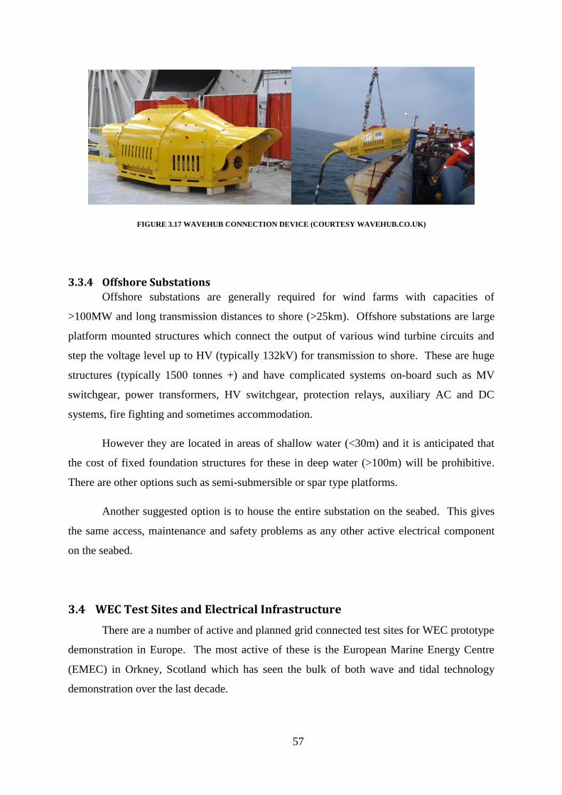
57
FIGURE 3.17 WAVEHUB CONNECTION DEVICE (COURTESY WAVEHUB.CO.UK)
3.3.4 Offshore Substations
Offshore substations are generally required for wind farms with capacities of
>100MW and long transmission distances to shore (>25km). Offshore substations are large
platform mounted structures which connect the output of various wind turbine circuits and
step the voltage level up to HV (typically 132kV) for transmission to shore. These are huge
structures (typically 1500 tonnes +) and have complicated systems on-board such as MV
switchgear, power transformers, HV switchgear, protection relays, auxiliary AC and DC
systems, fire fighting and sometimes accommodation.
However they are located in areas of shallow water (<30m) and it is anticipated that
the cost of fixed foundation structures for these in deep water (>100m) will be prohibitive.
There are other options such as semi-submersible or spar type platforms.
Another suggested option is to house the entire substation on the seabed. This gives
the same access, maintenance and safety problems as any other active electrical component
on the seabed.
3.4 WEC Test Sites and Electrical Infrastructure
There are a number of active and planned grid connected test sites for WEC prototype
demonstration in Europe. The most active of these is the European Marine Energy Centre
(EMEC) in Orkney, Scotland which has seen the bulk of both wave and tidal technology
demonstration over the last decade.

58
Although grid connected test sites are primarily designed for WEC prototyping, there
is the additional benefit of demonstration of the grid integration infrastructure and
measurement of power quality. Critically, however, the economics rationale for electrical
systems for test sites is not be as challenging as those for commercial projects.
An outline of some of the existing and planned wave energy test sites is given in this
section. This includes details of the electrical network within the test site, cable installation,
cable accessories, submarine connectors and operational experience if appropriate.
3.4.1 European Marine Energy Centre (EMEC)
EMEC has been in operation since 2003 and provides grid connected wave and tidal
facilities, scale test sites, site monitoring and office facilities to WEC developer clients. At
the Billia Croo wave test site EMEC provides seven grid connected berths, 5 offshore and 2
nearshore.
Figure 3.18 shows the layout of the wave test facility at EMEC. Each offshore berth
is connected by an 11kV submarine cable to shore. Offshore berths are located in
approximately 50-70m water depth and are 2km from shore. The nearshore berths are grid
connected onshore as the devices using these berths, Aquamarine Power and Seatricity,
utilise hydraulic transmission to shore.
The 11kV cables have 50mm2 conductors, dual steel armouring, pilot signal cables,
and fibre optic communications cables. The power cables are laid on the seabed from the
offshore berths to around 15m water depth. From here they are protected with ductile iron
cable protectors until they enter a trench at the shoreline. They are then connected to a local
11kV substation which is connected to the Orkney electrical grid. There are facilities at the
substation to operate the cables at other voltages than 11kV, e.g. Pelamis connect their
devices at 6.6kV at EMEC requiring a transformer onshore to step up the voltage to 11kV.
The offshore power cables are capped at the berth with one half of a submarine splice
housing, or connector, manufactured by J&S. WEC developers must connect a dynamic cable
from their WEC to the other half of the splice housing and make the final connection between
the two halves of the connector during WEC installation at the berth. The submarine
connector in use in EMEC is shown in Figure 3.19.

59
FIGURE 3.18 EMEC WAVE TEST SITE SCHEMATIC (SOURCE: EMEC.ORG.UK)
FIGURE 3.19 J&S SUBMARINE SPLICE HOUSING / CONNECTOR IN USE AT EMEC (COURTESY J&S LTD.)

60
EMEC is considered an extremely successful test site with multiple wave and tidal
devices prototyping at the site. The performance of the electrical system has been good with
lessons being learned in the protection of power cables and the use and reliability of
submarine connectors. EMEC have also developed guideline documents including a grid
connection guidance document [87].
3.4.2 Atlantic Marine Energy Test Site (AMETS)
The Sustainable Energy Authority of Ireland (SEAI) is planning a grid connected test
site, AMETS, off Annagh Head, near Belmullet, Co. Mayo, Ireland. AMETS will allow the
testing of pre-commercial WEC prototypes in extreme Atlantic conditions. SEAI are in the
advanced stages of securing a foreshore lease and planning permission for offshore and
onshore elements of the project.
AMETS plans to have two separate test areas, or berths. A deep-water berth (Test
Area A) will be located in 100m water depth and an intermediate depth berth (Test Area B)
will be located in 50m water depth. The deep-water berth is located around 16km from shore
and the intermediate berth is located around 6km from shore. Four 10kV submarine cables
will be installed to these berths, two to each berth. These four cables will be routed to a
substation at the head of Belderra Strand where they will be connected to a 10kV substation
and subsequently to the Irish electrical grid at 20kV. Some details of the proposed test site
are shown in Figure 3.20.
As AMETS has yet to be built the final details of the offshore electrical system, such
as cable specification and submarine connectors, are not finalised. AMETS will provide a
facility that experiences some of the most extreme conditions expected in the Atlantic for
WEC arrays. AMETS will provide an important proving ground for later stage WEC
prototypes.

61
FIGURE 3.20 SCHEMATIC SHOWING DETAILS OF AMETS TEST SITE (SOURCE: SEAI.IE)
3.4.3 Wavehub
Wavehub is a wave energy test site located off Hayle, on the Cornwall Coast in
southwest England. It consists of an electrical ‘hub’ on the seabed 16km from shore. The
hub is connected to an onshore substation by 25km of 33kV power cable, which is operated
presently at 11kV. From the onshore substation the site is connected to the electrical grid.
From the hub four berths are served, each in approximately 50m water depth with a capacity
for 4-5MW. If operated at 33kV Wavehub has the capacity for up to 50MW within the
existing infrastructure. A schematic of the site is shown in Figure 3.21.
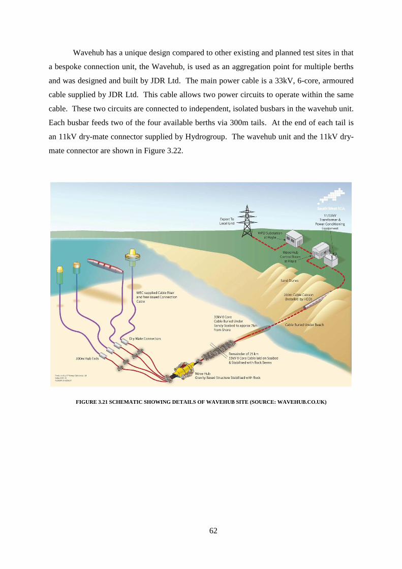
62
Wavehub has a unique design compared to other existing and planned test sites in that
a bespoke connection unit, the Wavehub, is used as an aggregation point for multiple berths
and was designed and built by JDR Ltd. The main power cable is a 33kV, 6-core, armoured
cable supplied by JDR Ltd. This cable allows two power circuits to operate within the same
cable. These two circuits are connected to independent, isolated busbars in the wavehub unit.
Each busbar feeds two of the four available berths via 300m tails. At the end of each tail is
an 11kV dry-mate connector supplied by Hydrogroup. The wavehub unit and the 11kV dry-
mate connector are shown in Figure 3.22.
FIGURE 3.21 SCHEMATIC SHOWING DETAILS OF WAVEHUB SITE (SOURCE: WAVEHUB.CO.UK)

63
FIGURE 3.22 WAVEHUB UNIT DURING INSTALLATION (L) AND HYDROGROUP DRY-MATE CONNECTOR (R)
(COURTESY WAVEHUB AND HYDROGROUP)
Although installed since 2010, Wavehub has not had any WEC prototype deployed at
the site at the time of writing. They have, however, had a number of WEC developers
expressing interest and designing prototypes for the site. More recently Wavehub have begun
to focus on offshore floating wind testing opportunities as an alternative use for the site.
3.4.4 Other Test Sites
Beyond the UK and Ireland there are a number of other wave energy test sites planned
around Europe.
3.4.4.1 Biscay Marine Energy Platform (BiMEP)
The Biscay Marine Energy Platform (BiMEP) is being developed by Ente vasco de la
Energía (EVE), a Basque government body. The site is located off the coast from Armintza,
Bizkaia, Spain. BiMEP has a total capacity of 20MW with four 13kV power cables
connected from an onshore substation to offshore ‘hubs’ which can feed multiple devices.
The exact design of the cables and these ‘hubs’ is not available at this time. A schematic of
the planned test site is given in Figure 3.23.
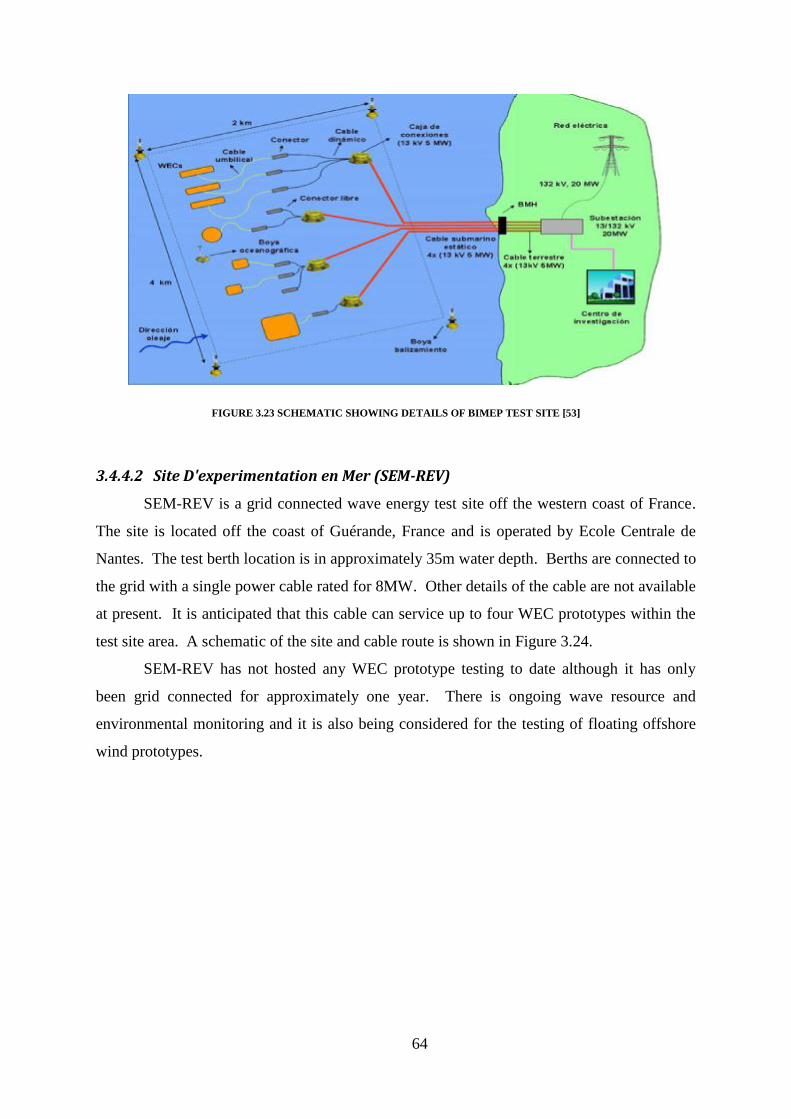
64
FIGURE 3.23 SCHEMATIC SHOWING DETAILS OF BIMEP TEST SITE [53]
3.4.4.2 Site D'experimentation en Mer (SEM-REV)
SEM-REV is a grid connected wave energy test site off the western coast of France.
The site is located off the coast of Guérande, France and is operated by Ecole Centrale de
Nantes. The test berth location is in approximately 35m water depth. Berths are connected to
the grid with a single power cable rated for 8MW. Other details of the cable are not available
at present. It is anticipated that this cable can service up to four WEC prototypes within the
test site area. A schematic of the site and cable route is shown in Figure 3.24.
SEM-REV has not hosted any WEC prototype testing to date although it has only
been grid connected for approximately one year. There is ongoing wave resource and
environmental monitoring and it is also being considered for the testing of floating offshore
wind prototypes.

65
FIGURE 3.24 SCHEMATIC OF SEM-REV TEST SITE LOCATION AND CABLE ROUTE (SOURCE: SEMREV.FR, ECOLE
CENTRALE NANTES)
3.4.4.3 Pilot Zone / Ocean Plug
In Portugal a test site for ocean energy has been proposed for a number of years. The
Pilot Zone, which is being developed by electrical utility REN, extends to 320km2 of leased
area off the coast north of Nazare, Portugal. The location of the project is shown in Figure
3.25.
The test site is expected to be developed in phases with the first phase consisting of
four 3MW berths connected at 15kV. Later, commercial phases are envisaged at the site up
to 250MW. The first phase is expected to have two, ‘interwoven’ cables from the shore to
the site area. From here the cables will be split into four individual links to the four 3MW
berths. Exact details of the connection scheme are not available at this time.
The project has obtained a concession (lease) for 45 years for the project area.
Projected timelines for the pilot zone are phase one by 2013; however some delays are
anticipated at this time.
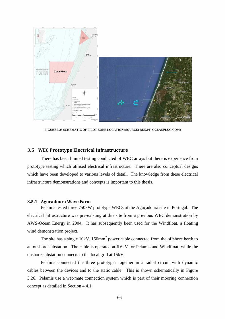
66
FIGURE 3.25 SCHEMATIC OF PILOT ZONE LOCATION (SOURCE: REN.PT, OCEANPLUG.COM)
3.5 WEC Prototype Electrical Infrastructure
There has been limited testing conducted of WEC arrays but there is experience from
prototype testing which utilised electrical infrastructure. There are also conceptual designs
which have been developed to various levels of detail. The knowledge from these electrical
infrastructure demonstrations and concepts is important to this thesis.
3.5.1 Aguçadoura Wave Farm
Pelamis tested three 750kW prototype WECs at the Aguçadoura site in Portugal. The
electrical infrastructure was pre-existing at this site from a previous WEC demonstration by
AWS-Ocean Energy in 2004. It has subsequently been used for the Windfloat, a floating
wind demonstration project.
The site has a single 10kV, 150mm2 power cable connected from the offshore berth to
an onshore substation. The cable is operated at 6.6kV for Pelamis and Windfloat, while the
onshore substation connects to the local grid at 15kV.
Pelamis connected the three prototypes together in a radial circuit with dynamic
cables between the devices and to the static cable. This is shown schematically in Figure
3.26. Pelamis use a wet-mate connection system which is part of their mooring connection
concept as detailed in Section 4.4.1.

67
FIGURE 3.26 SCHEMATIC REPRESENTATION OF PELAMIS ELECTRICAL NETWORK AT AGUÇADOURA (COURTESY
PELAMIS WAVE POWER)
3.5.2 AW Energy at Peniche
AW Energy deployed a nearshore WEC at Peniche in Portugal in 2012. This 300kW
‘Waveroller’ generates power on-board via a hydraulic PTO. The device is connected to
shore via a low voltage 1kV cable operating at 690V. The WEC is located in the nearshore
regime so the cable is approximately 1km in length.
3.5.3 Seabased at Lysekil
Seabased are a spin-out company from Uppsala University which develop linear
generator based WECs. Some detail is given in Section 3.3.3.2.3. They have operated a test
site at Lysekil since 2002 and have deployed numerous test prototypes. They have also
installed an underwater substation which houses power electronic converters and low voltage
switchgear. This low voltage marine substation (LVMS) is shown in Figure 3.27 along with
schematics for large LVMS and MVMS.
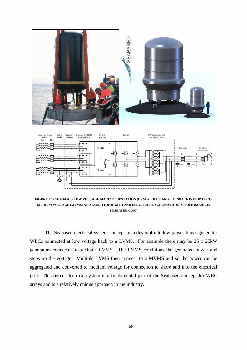
68
FIGURE 3.27 SEABASED LOW VOLTAGE MARINE SUBSTATION (LVMS) SHELL AND FOUNDATION (TOP LEFT),
MEDIUM VOLTAGE (MVMS) AND LVMS (TOP RIGHT) AND ELECTRICAL SCHEMATIC (BOTTOM) (SOURCE:
SEABASED.COM)
The Seabased electrical system concept includes multiple low power linear generator
WECs connected at low voltage back to a LVMS. For example there may be 25 x 25kW
generators connected to a single LVMS. The LVMS conditions the generated power and
steps up the voltage. Multiple LVMS then connect to a MVMS and so the power can be
aggregated and converted to medium voltage for connection to shore and into the electrical
grid. This tiered electrical system is a fundamental part of the Seabased concept for WEC
arrays and is a relatively unique approach in the industry.
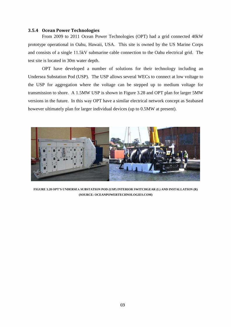
69
3.5.4 Ocean Power Technologies
From 2009 to 2011 Ocean Power Technologies (OPT) had a grid connected 40kW
prototype operational in Oahu, Hawaii, USA. This site is owned by the US Marine Corps
and consists of a single 11.5kV submarine cable connection to the Oahu electrical grid. The
test site is located in 30m water depth.
OPT have developed a number of solutions for their technology including an
Undersea Substation Pod (USP). The USP allows several WECs to connect at low voltage to
the USP for aggregation where the voltage can be stepped up to medium voltage for
transmission to shore. A 1.5MW USP is shown in Figure 3.28 and OPT plan for larger 5MW
versions in the future. In this way OPT have a similar electrical network concept as Seabased
however ultimately plan for larger individual devices (up to 0.5MW at present).
FIGURE 3.28 OPT’S UNDERSEA SUBSTATION POD (USP) INTERIOR SWITCHGEAR (L) AND INSTALLATION (R)
(SOURCE: OCEANPOWERTECHNOLOGIES.COM)

70
3.6 Offshore Wind Electrical Networks and Transfer to WEC Arrays
Offshore wind is a useful knowledge base for understanding the electrical networks
for WEC arrays. There are some applicable areas of transfer between the two, particularly
with the optimal configuration of WEC array electrical networks and installation processes.
There are also some key differences, particularly around the interface between the WEC and
the electrical network. This section outlines the potential areas of transfer and key
differences.
3.6.1 Offshore Wind Electrical Networks
Offshore wind farms have been commercially developed since the first, Vindeby
Wind Farm, was developed in 1991 off the coast of Lolland, Denmark. The main driver for
going offshore was for increased wind speeds and site availability [63]. Early offshore wind
farms utilised identical turbines to onshore wind farms although the components were
‘marinised’ and the foundation designs altered to allow for installation at sea. The electrical
system would also be identical to onshore wind farms with array cabling linked to a
substation (initially onshore and subsequently offshore) and connected to the electrical grid.
These early wind farms were built on shallow water sandbanks with typical water
depths <5m. Transmission distance to shore would also have been small (<5km). As larger
offshore wind farms were built they were pushed into deeper water areas further from shore
with offshore wind farms typically being installed presently in water depths of >20m with
transmission distances of >30km. Some of the characteristics of the world’s largest offshore
wind farms, as of 2013, are shown in Table 3.2.
The electrical network of a large offshore wind farm essentially consists of two
stages. There is a medium voltage (MV) array collection system, which is subsequently
connected to an offshore substation. This offshore substation steps the voltage up to high
voltage (HV) for export to shore. In the case of a HVDC connection the offshore substation
has a converter which converts the stepped up voltage from AC to DC.

71
TABLE 3.2 CHARACTERISTICS OF OFFSHORE WIND PROJECTS UP TO 2012 (SOURCE: 4COFFSHORE.COM AND
DEVELOPER WEBSITES).
What can be seen from Table 3.2 is that up to 2012 the majority of offshore wind
farms were installed less than 15km from shore and in less than 20m water depth. As the
installed capacity and distance from shore increased there was a requirement for offshore,
platform based, substations in order to step the voltage up to HVAC (>100kV) for
transmission to shore. Since 2010 there is a trend for offshore wind farms with much longer
transmission distances (up to 50km) and in deeper water (around 30m). This has meant
offshore wind farms with multiple offshore substations and/or multiple HVAC connections to
shore. With larger transmission distances and greater capacity some wind farms are
developing HVDC transmission systems such as the Borwin (400MW) and Helwin (576MW)
HVDC connection projects [88]. There are also development projects on deep-water wind
farms [89] and floating wind turbines [90].
Name Turbines Capacity Year
Distance
from Shore
/ POC
Max
Water
Depth
Inter
Array
Offshore
Substation
Shore
Connection AC / DC
# Cables
to Shore
London Array 175 630MW 2012 53km 25m 33kV Yes (2) 150kV HVAC 4
Greater Gabbard 140 504MW 2012 45km 32m 33kV Yes 132kV HVAC 3
Thornton Bank II 30 184MW 2012 39km 28m 33kV Yes 150kV HVAC 1
Sherringham Shoal 88 316MW 2012 22km 22m 33kV Yes 132kV HVAC 2
Ormonde 30 150MW 2012 43km 22m 33kV Yes 132kV HVAC 1
Walney Phase 2 51 183MW 2012 44km 30m 33kV Yes 132kV HVAC 1
Walney Phase 1 51 183MW 2011 43km 28m 33kV Yes 132kV HVAC 1
Thanet 100 300 MW 2010 11km 25m 33kV Yes 132kV HVAC 1
Rosand 2 90 207MW 2010 4km 10m 33kV Yes 132kV HVAC 1
Robin Rigg 60 180MW 2010 10km 9m 33kV Yes 132kV HVAC 1
Gunfleet Sands 48 172MW 2010 7km 15m 33kV Yes 132kV HVAC 1
Donghai Bridge 34 110MW 2010 10km 10m 35kV No 35kV MVAC 1
Vänern 10 30MW 2010 7km 22m 33kV No 33kV MVAC 1
Horns Rev 2 91 209 MW 2009 15km 17m 33kV Yes 150kV HVAC 1
Ryll Flats 25 90MW 2009 8km 12m 33kV No 33kV MVAC 3
Alpha Ventus 12 60MW 2009 45km 33m 30kV Yes 150kV HVAC 1
Lynn and Inner Dowsing 54 194MW 2008 5km 18m 33kV No 33kV MVAC 6
Princess Amalia 60 120MW 2008 23km 24m 22kV Yes 150kV HVAC 1
Lillgrund 48 110MW 2008 10km 8m 33kV Yes 138kV HVAC 1
Kemi Ajos 10 30MW 2008 11km 7m 20kV Yes 110kV HVAC 1
Thornton Bank I 6 30MW 2008 28km 27m 33kV Yes 150kV HVAC 2
Burbo Bank 25 90MW 2007 7km 8m 36kV No 36kV MVAC 3
Egmond aan Zee 36 108MW 2006 10km 18m 34kV No 34kV MVAC 3
Barrow 30 90MW 2006 27km 20m 33kV Yes 132kV HVAC 1
Kentish Flats 30 90MW 2005 8.5km 5m 33kV No 33kV MVAC 3
Nysted 72 166MW 2004 8km 12m 33kV Yes 132kV HVAC 1
Scroby Sands 30 60MW 2004 2.5km 15m 33kV No 33kV MVAC 3
Arklow Bank 7 25MW 2004 10km 5m 38kV No 38kV MVAC 1
North Hoyle 30 60MW 2003 7km 11m 33kV No 33kV MVAC 2
Samsø 10 23MW 2003 4km 13m 30kV No 30kV MVAC 1
Horns Rev 1 80 160MW 2002 14km 17m 36kV Yes 150kV HVAC 1
Mittelgrunden 20 40MW 2001 3.5km 6m 30kV No 30kV MVAC 1
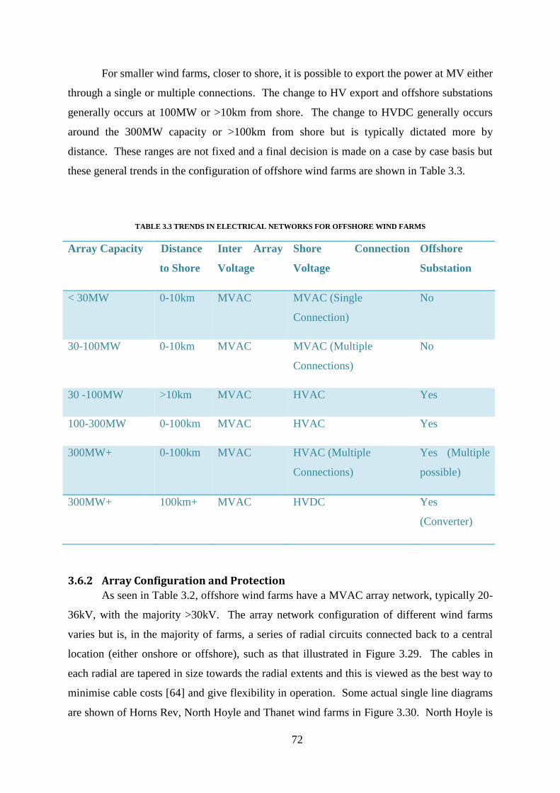
72
For smaller wind farms, closer to shore, it is possible to export the power at MV either
through a single or multiple connections. The change to HV export and offshore substations
generally occurs at 100MW or >10km from shore. The change to HVDC generally occurs
around the 300MW capacity or >100km from shore but is typically dictated more by
distance. These ranges are not fixed and a final decision is made on a case by case basis but
these general trends in the configuration of offshore wind farms are shown in Table 3.3.
TABLE 3.3 TRENDS IN ELECTRICAL NETWORKS FOR OFFSHORE WIND FARMS
Array Capacity Distance
to Shore
Inter Array
Voltage
Shore Connection
Voltage
Offshore
Substation
< 30MW 0-10km MVAC MVAC (Single
Connection)
No
30-100MW 0-10km MVAC MVAC (Multiple
Connections)
No
30 -100MW >10km MVAC HVAC Yes
100-300MW 0-100km MVAC HVAC Yes
300MW+ 0-100km MVAC HVAC (Multiple
Connections)
Yes (Multiple
possible)
300MW+ 100km+ MVAC HVDC Yes
(Converter)
3.6.2 Array Configuration and Protection
As seen in Table 3.2, offshore wind farms have a MVAC array network, typically 20-
36kV, with the majority >30kV. The array network configuration of different wind farms
varies but is, in the majority of farms, a series of radial circuits connected back to a central
location (either onshore or offshore), such as that illustrated in Figure 3.29. The cables in
each radial are tapered in size towards the radial extents and this is viewed as the best way to
minimise cable costs [64] and give flexibility in operation. Some actual single line diagrams
are shown of Horns Rev, North Hoyle and Thanet wind farms in Figure 3.30. North Hoyle is

73
unusual in that the network has some redundancy built into the design which is discussed in
Section 3.6.3. Thanet shows a more optimised forked radial configuration which has a
centrally located offshore substation and multiple forked radials which minimises the cost of
the electrical network.
FIGURE 3.29 TYPICAL OFFSHORE WIND FARM ELECTRICAL ARRAY CONFIGURATION (COURTESY ABB)
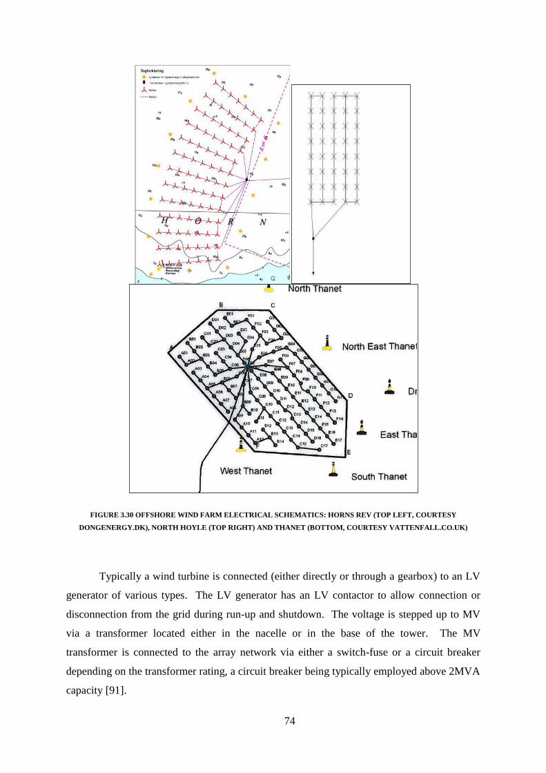
74
FIGURE 3.30 OFFSHORE WIND FARM ELECTRICAL SCHEMATICS: HORNS REV (TOP LEFT, COURTESY
DONGENERGY.DK), NORTH HOYLE (TOP RIGHT) AND THANET (BOTTOM, COURTESY VATTENFALL.CO.UK)
Typically a wind turbine is connected (either directly or through a gearbox) to an LV
generator of various types. The LV generator has an LV contactor to allow connection or
disconnection from the grid during run-up and shutdown. The voltage is stepped up to MV
via a transformer located either in the nacelle or in the base of the tower. The MV
transformer is connected to the array network via either a switch-fuse or a circuit breaker
depending on the transformer rating, a circuit breaker being typically employed above 2MVA
capacity [91].

75
In most cases the connection to the cable is done through a simple switch disconnect
with a cable earthing facility although in some cases a direct connection to the cable from the
busbar is employed, sometimes a combination of the two (see Figure 3.32) to reduce cost.
Some typical connection arrangements are shown in Figure 3.31.
FIGURE 3.31 TYPICAL GENERATOR AND SWITCHGEAR ARRANGEMENTS FOR OFFSHORE WIND.
Figure 3.31 (a): Transformer protection: MV switch fuse
Cable connection: switch-disconnect.
Figure 3.31 (b): Transformer protection: MV circuit breaker
Cable connection: switch-disconnect.
Figure 3.31 (c): Transformer protection: MV circuit breaker
Cable connection: direct connection.

76
In the event of a cable fault the cable is protected by the MV fuse or circuit breaker.
This disconnects the wind turbine generator and the circuit breaker at the substation (i.e. the
beginning of the radial) thus disconnecting the fault from the electrical grid. The cable
switch-disconnects are used for isolating (and earthing) a cable for maintenance, and post
fault.
FIGURE 3.32 TYPICAL CONNECTION FOR OFFSHORE WIND FARM RADIAL
For example in Figure 3.32, (which shows a combination of cable switch disconnect
and direct connection) if a fault occurred at point ‘A’ on the submarine cable between WTG3
and WTG4, the main circuit breaker at the offshore substation connected to WTG7 would
open and the generators (1-7) would be disconnected from the network. The faulty cable
would be isolated by opening the cable switch in WTG4. Then the radial could be re-
energised from the offshore substation, however only WTG 5, 6 & 7 could generate as the
radial circuit is now broken until the cable can be repaired. This results in lost generation
capacity and is an inherent weakness of radial network configurations. Also as the generators
are all disconnected for the fault at point ‘A’, there is also lost generation during the
reconfiguration of the radial after the fault. In order to overcome this some redundancy and
sectionalising have been proposed.

77
3.6.3 Redundancy and Sectionalising
Yang et al concluded [68] that with reasonable investment in redundancy the
reliability of an offshore wind farm improves. Ackermann presents a selection of layouts for
offshore collector systems [63] introducing different redundancy concepts, shown in Figure
3.33.
Redundancy in the circuit can be achieved in a variety of ways, the simplest being the
connection of two radials together at their extents. However, this means that each radial must
(in a worst case scenario) carry the additional rated power from the other radial, meaning a
requirement for larger cables in both radials. Therefore the increased security and reliability
comes at the expense of additional, larger cables and switchgear. A compromise can be
achieved by not rating the redundant cabling at full capacity and curtailing generation to the
circuit limit should that limit occur while the alternative circuit is in place. This allows a
reduction in cable size in the redundant circuit. To date the vast majority of offshore wind
farms have employed a simple radial circuit with no redundancy, this being viewed as the
most economical option.
FIGURE 3.33 REDUNDANCY CONCEPTS FOR OFFSHORE WIND FARM ARRAYS

78
In [65] Franken et al establish that increased availability can be achieved using
redundant circuits, however this availability can be increased further given a sectionalising
approach to protection. Franken et al conclude that the equivalent of up to 2 wind turbines
generated annual energy can be saved with the addition of redundancy and sectionalising.
This was based on a 160MW wind farm (40 x 4MW Turbines).
3.6.4 Submarine Cable Installation
The method of cable installation in an offshore wind farm has developed rapidly with
the evolution of the industry and there are now custom built vessels for this purpose. The
total cable installation consists of the following steps (considering a wind farm with offshore
substation)
1. Transmission cable shore end operation
2. Transmission cable to offshore substation installation
3. Transmission cable pulling into offshore substation
4. Array cable installation
5. Array cable pulling into turbine bases
6. Array cable pulling into offshore substation
This is completed with a combination of ships, barges, ROVs, ploughs, and divers.
From a WEC array perspective steps 1, 2 and 4 would be identical as to an offshore wind
farm, although there will be some site specific constraints and peculiarities. Therefore the
areas of interest are steps 3 and 5.
Step 3: This involves the pulling of the cable using a pull wire into the substation
through a j-tube. The cable is installed up to a point adjacent to the substation base and extra
cable is played out onto the seabed (to allow for connection into the substation). The cable is
then cut and a pulling nose fitted to the cable end. From the offshore substation a pull wire is
passed down the j-tube where it is picked up (by ROV or diver.) and connected to the cable

79
pulling nose. The cable is then winched up into the offshore substation where it is prepared
for termination to the switchgear.
Step 5: This involves the pulling of the cable using a pull wire into the wind turbine
base through a j-tube. The cable is installed up to a point adjacent to the wind turbine base
and extra cable is played out onto the seabed (to allow for connection into the wind turbine).
The cable is then cut and a pulling nose fitted to the cable end. From the wind turbine a pull
wire is passed down the j-tube where it is picked up (by ROV or diver) and connected to the
cable pulling nose. The cable is then winched up into the wind turbine where it is prepared
for termination to the switchgear.
For the cable installation, the use of specialist vessels and equipment is critical. The
cable installation and protection depends on numerous factors including the location, seabed
conditions, and expected marine traffic. The cable installation process cost can typically be
higher than the cable cost itself [66], sometimes a multiple of the cable cost.
There are several possible methods of cable installation which are briefly outlined
below:
1. Cable installation on seabed: This is the simplest installation procedure whereby the
cable is laid onto the seabed and simply kept in place by its own weight. This would
rarely be used for power cables in offshore wind farms as the cables are subject to
damage by currents, trawlers, anchorage and marine life. It is used in very deep water
for long distance communications cables.
2. Pre trenching and installation: This method involves trenching before the cable is
installed and then installing the cable into the trench and closing the trench. This
procedure is not normally utilised in offshore wind farms.
3. Cable installation and post installation trenching: This method involves the cable
being installed on the seabed. Following installation the cable is trenched and buried
to a specified depth. The trenching and burial is normally undertaken by an ROV
using a jetting system. This is the normal procedure for installing short lengths of
cable in shallow water such as the infield cables in an offshore wind farm.
4. Combined cable installation and burial: This method involves the cable being
installed on the seabed, trenched and buried simultaneously. The trenching and burial
is undertaken with a plough which is towed behind the cable installation vessel. This

80
is the normal procedure for installing long lengths of cable in shallow water such as
the transmission cable to shore in an offshore wind farm.
5. Cable installation and post protection: This method involves the cable being installed
on the seabed. Following installation the cable is protected using rock dumping or
concrete mattresses. This is suitable for where the seabed conditions do not permit
burial or where the cable must cross over another cable/pipe.
6. Cable installation and pre protection: This method involves some mechanical
protection being installed on the cable as it is installed. This protection could be some
ducting system like Uraduct. This is used for specialised protection application such
as the touchdown point where the cable enters the wind turbine J-tube and may be
subject to scouring.
7. Horizontal Directional Drilling: This method involves HDD from shore to a
connection point. A duct is then inserted into the HDD hole and the cable is drawn
through the duct. The length of the HDD is limited to a few km so it is not practical
for offshore wind farms. It has been used for tidal energy devices due to the high
currents in the area of installation.
Array cabling is normally installed using method 3 whereby the cable is laid and
subsequently buried. Method 5 or 6 may be used for the exposed part of the array cable
around the J-tube to reduce scour or cable damage at the J-tube entrance.
Export cabling is normally installed using method 4 whereby the cable is laid and
simultaneously buried. Method 5 or 6 may be used for the exposed part of the cable around
the J-tube (at the offshore substation) to reduce scour or cable damage at the J-tube entrance.
The shore end of the cable is normally floated to shore, using buoyancy modules, and
then buried after installation by excavators or by ROV to the low water line.
The main section of the cable is installed by a cable plough. The cable plough can
start to install the cable from the high water line. The plough is pulled behind the cable lay
vessel and simultaneously cuts a trench and lays the cable in this trench. There are two types
of cable plough, displacement and non displacement. Displacement ploughs cut a large
trench and lay the cable in the trench which is subsequently backfilled. Non-displacement

81
ploughs cut a small slice into the seabed with a blade like ‘shear’. The cable is
simultaneously fed into this slice and immediately buried as the slice naturally closes in.
Ploughs can bury cables in a larger variety of seabed soils than jetting ROVs including hard
clays and loose shale or stones.
3.6.5 Offshore Substations
For wind farms with capacities of >100MW or sometimes transmission distances of
>10km an offshore substation is required to step up the MV array voltage to HV for export.
This reduces export losses and export cable sizes. It is not practical that the voltage could be
stepped up to HV in each of the turbines. In order to collect the power from the radials in the
wind farm and step it up to HV an offshore substation is required.
An offshore substation typically contain the following components:
MV Switchgear for collection of the array power
Oil Filled Step Up Transformer to step the voltage up to HV for connection to
shore
Fire and Blast Protection for Transformer
HV Switchgear for protection and isolation of transformer and HV export cable
Line Reactors
Protection and Metering Relays
Auxiliary and Emergency Power Systems
Accommodation Quarters and Workshop facilities
Medical and Rescue Equipment
Helipad
For HVDC systems the offshore substation also contains the converter to convert the
voltage from HVAC to HVDC for export. HVDC offshore substations are significantly
larger and heavier as a result.
HVAC offshore substations are delivered as a single unit and can weigh over 2000t
and have an area of up to 800m2. Typically a single HVAC offshore substation would be

82
rated for a maximum of 500MW. For large wind farms multiple substations are required
each with their own export cable to shore giving some redundancy to the export system.
HVDC offshore substation can weigh more than 10,000t and are beyond the
capability of most heavy lift vessels. These platforms must be self installing structures which
are floated to site and jacked up into position. HVDC offshore substations up to 690MW are
installed with individual platforms up to 900MW in planning.
Offshore substation foundations can be similar to that for an offshore wind turbine
although with a different load pattern. For small offshore substations a monopile foundation
is suitable. For large offshore substations distributed piles or a jacket foundation is more
suitable. For very large HVDC offshore substation the foundation must self install as no
heavy lift is possible for this scale of substation. Some photos of offshore substations are
shown in Figure 3.34.
FIGURE 3.34 OFFSHORE SUBSTATIONS (FROM TOP LEFT CLOCKWISE) – BARROW (2006, 450T, 90MW, COURTESY
WIKICHOPS), SHERRINGHAM SHOAL (2011, 875T, 316MW), BORWIN BETA (HVDC – SELF INSTALL) (2014, 10,000T,
800MW, COURTESY WAERFELU). DOLWIN BETA (HVDC – SELF INSTALL) (2014, 20,000T+, 900MW, COURTESY STEN
DUELAND)

83
3.6.6 HVDC Transmission for Offshore Wind
The first HVDC links of significant scale were developed in the 1970s and the
transmission technology has developed significantly in the intervening decades. HVDC
systems do not suffer from reactive losses and so are more suitable for long distance,
however as they require a converter station at both ends they are expensive relative to HVAC
and therefore they are only economical for large capacities/distances. HVDC links were
initially used to connect remote generators (such as hydroelectric stations) to load centres,
interconnecting countries, and also connecting systems of different frequencies (such as the
south and north of Japan). In recent years, however, they have gained attention for
connecting large offshore wind farms due to the increasing capacity and export distances for
planned wind farms.
HVDC systems can be broken into two categories, LCC (Line Commutated
Converter) and VSC (Voltage Source Converter)
LCC Systems have the advantage that they have a long and proven track record with
most HVDC systems installed in the world being LCC based. They have the disadvantage of
requiring a large footprint due to the component size and also requiring a very stable AC grid
at both ends to operate. For offshore wind farms this can mean a diesel generator or StatCom
(Static Compensator) is required to support the offshore grid in times of low wind. LCC
systems have an overall efficiency of 97-98%.
The basic LCC system uses monopole transmission, i.e. a single cable is used with the
sea as the return path. This reduces system cost but has other negative effects such as
electrochemical reactions on other subsea services such as gas pipelines, electro-chlorination
and navigation impact on ships. This is not normally acceptable so a monopole with a
separate of integrated return path is normally used for monopole configurations (see Figure
3.35). The other option is to use a bipole configuration which requires two separate HVDC
cables but allows a larger voltage across the two poles, as one is positive and the other is
negative.
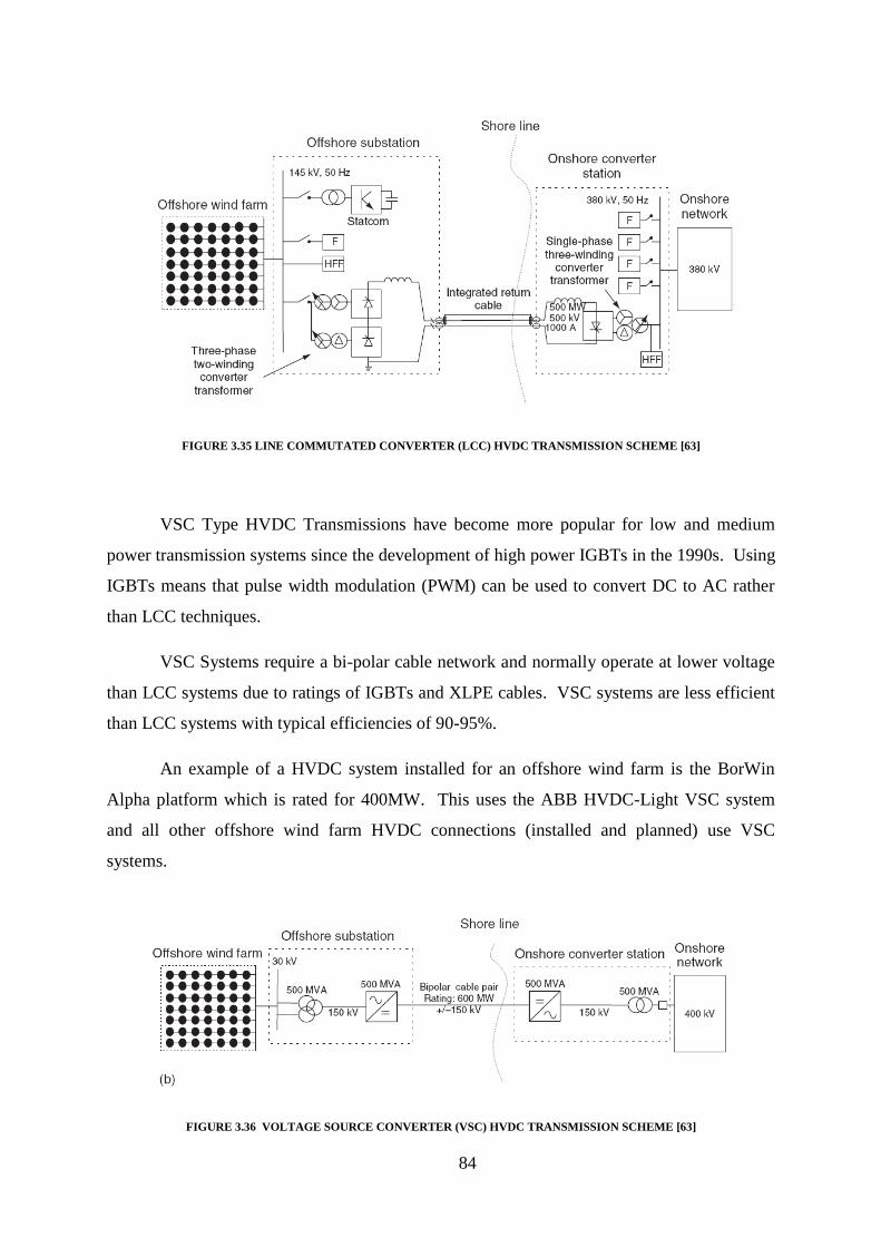
84
FIGURE 3.35 LINE COMMUTATED CONVERTER (LCC) HVDC TRANSMISSION SCHEME [63]
VSC Type HVDC Transmissions have become more popular for low and medium
power transmission systems since the development of high power IGBTs in the 1990s. Using
IGBTs means that pulse width modulation (PWM) can be used to convert DC to AC rather
than LCC techniques.
VSC Systems require a bi-polar cable network and normally operate at lower voltage
than LCC systems due to ratings of IGBTs and XLPE cables. VSC systems are less efficient
than LCC systems with typical efficiencies of 90-95%.
An example of a HVDC system installed for an offshore wind farm is the BorWin
Alpha platform which is rated for 400MW. This uses the ABB HVDC-Light VSC system
and all other offshore wind farm HVDC connections (installed and planned) use VSC
systems.
FIGURE 3.36 VOLTAGE SOURCE CONVERTER (VSC) HVDC TRANSMISSION SCHEME [63]

85
The choice of when to use HVDC over HVAC depends on numerous factors
including the overall cost of the solution. However the predominant factors are the capacity
of the wind farm and the distance to shore. The likely transmission concept for a
combination of these two factors is shown in Figure 3.37. As can be seen any offshore wind
farm with an installed capacity over 400MW or a distance of greater than 100km from shore
would be considered a candidate for HVDC transmission. In reality any wind farm with a
transmission distance of greater than 100km would need to have a capacity greater than
400MW for a variety of other economic reasons. The choice between HVAC and HVDC at
the extents of these limits will be down to cost and efficiency.
FIGURE 3.37 TRANSMISSION CONCEPTS BASED ON DISTANCE (TO SHORE) AND CAPACITY OF OFFSHORE WIND
FARMS [63]
There are still risks associated with the availability of these HVDC systems as they
introduce numerous additional ‘active’ electrical systems which have multiple failure modes.

86
3.6.7 Efficiency of Offshore Wind Collection and Transmission Systems
In [92], [70]& [93] the active power losses and efficiency of offshore wind farms are
evaluated and it is shown that up to 98% efficiency can be achieved for certain theoretical
configurations, however 96-97% is more typical for the majority of offshore wind farms
which have a similar electrical configuration as shown in Figure 3.29.
3.7 Crossover and Differences between Offshore Wind Farms and WEC
Array Electrical Networks
There is certainly a crossover of knowledge possible between offshore wind farm and
WEC array electrical network design. This is particularly so in the selection of optimal
network configuration, export solutions for various scales of WEC arrays, submarine cable
installation processes, and offshore substation design.
Offshore wind farms electrical network configurations have converged on radial
designs. More recently optimisation programmes are used to give the most efficient and
lowest cost electrical network and locate the offshore substation for same. The rationale for
radial networks is primarily economic as the literature has shown that redundant network
configurations would increase availability.
Cable installation procedures and vessels for offshore wind will, for the most part
cross over to WEC arrays. WEC array sites, as will be shown, may be in deeper water and
more energetic locations. This is a challenge for WEC array electrical networks which is
discussed in Chapter 5.
The export solutions for a range of offshore wind farm capacities and transmission
distances (Table 3.3) will be relevant to WEC array electrical networks and this is reflected in
Chapter 4.
There are key differences between offshore wind farm and WEC array electrical
network design. These are outlined briefly below and solutions to deal with these are
presented in later sections.
1. At present the majority of WEC prototypes are rated around 1MW. This is a
lower rating than a typical offshore wind turbine which is rated around 3-4MW

87
with larger turbines in development. Smaller individual WEC ratings will present
challenges for the economic design of WEC array electrical networks
2. WEC designs are divergent unlike offshore wind turbines, which are almost all
three bladed, horizontal axis. This can mean that a generic solution for WEC
array electrical networks will be more challenging until such time as WEC
technology designs converge.
3. Some ‘direct drive’ WEC concepts have a high peak to average output power
ratio, i.e. a low capacity factor. This presents challenges for the economic design
of WEC array electrical networks and also may cause power quality issues (See
Chapters 5 and 6)
4. The water depth at potential WEC array sites is likely to be much deeper than
offshore wind sites which presents challenges for offshore substation foundation
design and also for submarine cable installation.
5. In order to access deeper water depths the export distance to shore may be greater
for WEC arrays. This is geographically dependent.
6. Unlike offshore wind farms, in WEC arrays the devices require removal from site
for maintenance activities. This requires connection and disconnection
functionality but also may break the electrical circuit for upstream devices.
7. WECs are not fixed structures like offshore wind turbines and therefore require
dynamic cable connections to the electrical network
8. The array spatial configuration for WEC arrays is driven by different factors than
that of an offshore wind farm.
9. As WEC array sites are high energy wave sites the installation and protection of
submarine cable systems will be challenging
10. WEC technology is not proven onshore, as is the case with offshore wind.
Therefore smaller initial WEC arrays are expected which will be economically
challenging.
In the next Chapter the state of the art technologies for WEC arrays and the crossover
knowledge from offshore wind will be utilised to undertake a techno-economic optimisation
of WEC array electrical networks

88
3.8 Conclusion
Electrical network design for WEC arrays is a novel research problem but is critical to
the delivery of cost effective WEC arrays. An understanding of the electrical components
and systems on-board the WEC devices, within the WEC array electrical network, and any
experience from WEC test sites or WEC prototypes is invaluable for developing a techno-
economic analysis of future WEC array electrical networks. Some of these electrical
networks for test sites and prototypes may have developed sub-optimally and show signs of
divergence in configuration, components and concept.
The offshore wind industry is relatively mature and electrical network designs have
converged. There is certainly opportunity for cross-over of knowledge from offshore wind to
wave industries. However, the differences and novel challenges which WEC array electrical
networks present must be acknowledged and addressed.
There are key differences between offshore wind and WEC array electrical networks.
These differences are primarily in the areas of device ratings, site characteristics,
maintenance strategies and around the key interfaces between the WEC and the electrical
network. Optimising these key interfaces to allow for the required functionality but at an
acceptable cost is explored in the next chapter.
89
4 Techno-economic Analysis of Electrical Networks for WEC Arrays
Chapter 4
Techno-economic Analysis of Electrical
Networks for WEC Arrays
4.1 Introduction
There is minimal experience in the wave energy or utility industry of designing and
installing electrical networks for WEC arrays, with the closest comparison being offshore
wind farms. The offshore wind industry has developed to the stage that very large wind
farms (>500MW) have been installed, with larger projects in development. There is some
potential knowledge transfer from offshore wind to WEC array electrical network design as
outlined in Chapter 3. It has been shown also, in Chapter 3, that there are some key
differences between the array electrical network requirements of both offshore wind and
wave, which require original designs to be developed.
In this chapter, a techno-economic analysis of electrical networks for WEC arrays is
undertaken. Critical design factors, constraints, and assumptions are examined by
considering WEC array layout factors, economic and performance targets, and key interfaces
between the WEC and the array electrical network.
4.1.1 Technical, Functional and Economic Factors
Techno-economic analysis must consider the economic, technical and functional
factors in the context of the cost competitiveness of the entire solution. These are listed
below but outlined in detail in the subsequent sections.
Economic factors include:
o Capital cost of equipment
o Installation costs
o Operational costs
o Decommissioning costs

90
Technical factors include:
o WEC ratings
o Capacity factor
o Array Scale
o Site characteristics (water depth, distance to shore)
o Array spatial layout
o Key interfaces
Functional factors include:
o Connection and disconnection for installation and maintenance
o Continuity of network during maintenance and faults
o Safe operability
o Electrical protection
The factors given above must be considered when optimising the design of the
electrical network for WEC arrays. A balance must be struck between a technically superior
solution and one which is economically competitive. For WEC test facilities, such as those
described in Section 3.4, the balance is in favour of technically superior solutions as there is
less commercial pressure on the electrical network design.
The scale of the array being evaluated must also be considered. One challenge for
WEC arrays is that the technology is novel and cannot be proven onshore. Therefore it is
likely that smaller arrays, perhaps less than 10MW, will be required initially. Early offshore
wind projects took proven onshore technologies into the offshore environment and therefore
did not require small initial wind farms to prove the technology. These smaller arrays will
challenge the economics further as economies of scale cannot be achieved.
4.1.2 Methodology
As outlined there are many factors which must be considered for a techno-economic
analysis of WEC array electrical networks. The methodology for optimisation is outlined
below and in Figure 4.1 and ensures that all design requirements, constraints and assumptions
are considered in the development of optimal electrical networks for WEC arrays.

91
FIGURE 4.1 GRAPHICAL REPRESENTATION OF TECHNO-ECONOMIC OPTIMISATION PROCESS
The first step is to analyse wave energy in the European market context to understand
what the competitive costs for wave energy are. From this the available, or target CAPEX for
Capex Information
from Offshore Wind
Defined Capex
Target
Offshore Wind Electrical
Network Knowledge and
Key Differences to WEC
array electrical networks
Candidate WEC
Arrays for Analysis
Definition of WEC
Array Design
Criteria
Analysis of the State of the
Art in WEC array design to
provide constraints and
assumptions
Definition of WEC
Array Functional
Requirements
Analysis of Key
Interface
Alternatives
Analysis of Array
Electrical Network
Configurations
Submarine Cable
Cost Model
Techno-Economic
Optimisation
Inputs to Optimisation Optimisation Steps

92
electrical systems can be estimated. This target cost guides the optimisation process from an
economic aspect.
An analogue to WEC array electrical networks is the evolution of electrical networks
for offshore wind, which was analysed in Chapter 3. This examined how designs converged
and the driving factors behind this convergence. Importantly, while analysing where offshore
wind can cross over to wave energy, the key differences have been identified between the
two. Solutions which allow for these key differences while acknowledging crossover areas
will be critical to the optimisation process.
The technical and functional factors which are outlined briefly in Section 4.1.1 are
analysed in detail. This provides an understanding of the characteristics of a WEC array in
terms of array spatial layout, device separation, water depth, distance from shore, WEC
nameplate ratings, and capacity factors amongst others. Some assumptions must be made
here to allow for an optimisation process, and these are outlined.
The functional requirements and constraints as outlined in Section 4.1.1 are analysed
in detail. Examples include installation requirements, operational requirements, maintenance
requirements, and protection/safety requirements.
Critical design elements are the key interfaces between the WEC and the array
electrical network. Components at these interfaces can fulfil connection and disconnection
functions, in addition to protection functions. The components at the key interface include
submarine connectors, switchgear, and hull penetrations. These are critical but potential high
cost components. There are a variety of potential methods for realising these components
and these methods are also analysed in the context of the overall WEC array electrical
network cost and functionality.
Using all the analyses from the previous steps, a techno-economic optimisation of the
array electrical network can be undertaken, and suitable designs evaluated from an economic,
technical and functional perspective. This allows an optimised design to be selected for
further analysis.
The optimised electrical network design can be evaluated for efficiency at various
voltage levels, with efficiency calculated over the annual output of a typical WEC allowing
the annual energy losses to be calculated for a typical array.

93
Throughout this chapter the techno-economic optimisation and subsequent evaluation
is undertaken using a combination of statistical analysis, frequency domain analysis, time
domain analysis, and economic modelling. In some cases some subjective analysis of
alternatives is undertaken under predetermined criteria.
4.2 Wave Energy Cost Breakdown and Target Cost
Electrical systems for offshore wind farms can typically cost 20-25% of the overall
system CAPEX [2], and the same is anticipated for commercial WEC arrays [3]. For pre-
commercial arrays the percentage of CAPEX for electrical systems will be lower as the cost
of the actual converters will be much higher. Renewable UK [12] expects investment costs
of offshore wind to remain at circa £3m/MW (~€4m/MW) up to 2022 with levelised cost of
energy (LCoE) reducing to £130/MWh (€160/MWh) during that period.
As outlined in Chapter 1 wave energy must be competitive with other comparable
renewable energy sources if it is to obtain a significant market. So if the target cost of WEC
arrays is that of offshore wind farms and the proportion of that cost for electrical systems is
20-25% of the overall cost then the following costs for WEC array electrical systems would
be expected. This assumes that similar capacity factors can be achieved for wave farms as
for current offshore wind farms.
Wave Energy Target Installed Costs: €4 m/MW [12]
WEC Array Electrical Systems Target Costs: €1m/MW (25% of the above)
Therefore the electrical system in the WEC array must cost less than €1m/MW to be
comparable in cost to offshore wind. Although the cost of the WEC is expected to come
down dramatically as the industry reaches maturity, the cost of the electrical elements are
predominantly mature at present as mature technologies are expected to be utilised. There
are however some design criteria which may increase the electrical system costs and also
some potential strategies for reducing costs which are discussed in Chapter 5.
The challenge, and objective of this section, is to design a WEC array electrical
network which can provide the required functionality within the technical and economic
constraints outlined.

94
4.3 WEC Array Design Considerations, Constraints and Assumptions
To facilitate the techno-economic analysis of WEC array electrical networks this
section outlines major design considerations, technical constraints and working assumptions
for the WEC array. This information, coupled with the state-of-the-art knowledge from
offshore wind electrical network design shown in Section 3.6, allows the development of a
credible outline and roadmap for wave energy converter arrays. The following sections
describe important factors in this optimisation.
4.3.1 The Wavebob Wave Energy Converter
The WEC used as a candidate for part of this research is the Wavebob device shown
in Figure 4.2. However, the results and conclusions are generally applicable to any deep-
water floating WEC. The results may also be somewhat applicable to other types of WEC,
floating offshore wind and tidal energy converter arrays.
FIGURE 4.2 1:4 SCALE WAVEBOB DEVICE IN GALWAY BAY (L) AND DEVICE DRAWING (COURTESY WAVEBOB
LTD.)
The Wavebob device is a self reacting point absorber type WEC [4]. The device is
made up of two main structures, the torus and the float-neck-tank (FNT), connected by a
power take off (PTO) system. This device has been tested at various scales up to 1:4 scale.

95
A full scale device was planned for deployment off the west coast of Ireland2. The general
characteristics for the full scale Wavebob device are given below.
Geometry: Torus Diameter: 22m, Height: 65m, Freeboard: 20m
Design water depth: >100m
Device Electrical Rating: 1MW
4.3.2 Site Locations
The full scale Wavebob device is designed for operation off the west coast of Ireland
in >100m water depth. The 100m contour off the west coast of Ireland is shown in Figure
4.3. The 100m contour mostly lies between 10km and 25km from the nearest landfall
depending on the location. Areas of counties Mayo, Galway and Kerry have landfall within
10km of the 100m contour and may be utilised in the first deep-water arrays, although there
will also be an emphasis on the availability of grid connection capacity, which may be better
in some locations. Later arrays can be expected to be more than 20km from landfall.
2 In 2013 Wavebob was put into administration and the technology development has not continued as
planned

96
FIGURE 4.3 100M DEPTH CONTOUR (FIRST RED LINE OFF THE WEST COAST OF IRELAND) [SOURCE MIDA]
4.3.3 Resource and Generation Distribution
To understand the generation characteristics of the Wavebob WEC off the west coast
of Ireland the scatter diagram from the Belmullet test site off the coast of Mayo, Ireland is
analysed in detail and the Wavebob frequency domain model is utilised. The scatter diagram
is shown in Figure 4.4. The scatter diagram shows the occurrences (in the case below
10,000) of significant wave height, Hs, and wave period, Tp, over a particular period
(typically one year). The scatter diagram characterises the resource at a particular site.

97
FIGURE 4.4 BELMULLET SCATTER DIAGRAM [94]
Using this scatter diagram and a frequency domain simulation model of the Wavebob
device, the distribution of the annual generated power for the Wavebob device at the
Belmullet site is determined. Two results of interest are shown in Figure 4.5 and Figure 4.6.
FIGURE 4.5 WAVEBOB AT BELMULLET - ANNUAL DISTRIBUTION OF ENERGY YIELD BY % OUTPUT
0.00%
5.00%
10.00%
15.00%
20.00%
25.00%
0-10 10-20 20-30 30-40 40-50 50-60 60-70 70-80 80-90 90-100
Ene
rgy
Yie
ld (
%)
Generated Power (% Output)
Annual Energy Yield (MWh) Distribution

98
FIGURE 4.6 WAVEBOB AT BELMULLET - ANNUAL DISTRIBUTION OF GENERATION HOURS BY % OUTPUT
Figure 4.5 and Figure 4.6 illustrate the generation characteristics of the Wavebob
WEC at the Belmullet site. It can be seen, in Figure 4.5, that ~45% of the annual energy
yield is produced when the WEC generates above 70% of the rated power. Also, in Figure
4.6, it can be seen that the WEC generates below 70% of rated output for ~80% of the year.
Therefore ~45% of the energy comes from ~20% of the operation time.
An understanding of this variability allows the calculation and optimisation of the
efficiency of the WEC array electrical network in Section 4.7.
4.3.4 Array Spatial Configuration
The spatial configuration of an array of WECs will be determined from a number of
factors, including:
1. Maximising energy capture and reducing destructive interference
2. Minimising the overall area used by the array and taking account of local bathymetry
0.00%
5.00%
10.00%
15.00%
20.00%
25.00%
0-10 10-20 20-30 30-40 40-50 50-60 60-70 70-80 80-90 90-100
Ge
ne
rati
on
Ho
urs
(%
)
Generated Power (% Output)
Annual Generation Hours Distribution

99
3. Mooring footprint and installation requirements
4. Marine operations such as vessel access for deployment and maintenance
5. Reduction in electrical losses and cable costs
The spatial configuration and device interaction of WEC arrays is a critical research
topic for wave energy. C. Fitzgerald and Thomas [72] reference the q-factor, which is the
ratio of the absorbed energy by a single device versus the absorbed energy from the same
device operating within an array, i.e. its ‘array efficiency’. Where q > 1 constructive
interference is taking place within the array; where q < 1 destructive interference is taking
place. Ricci et al. conclude [76] that device performance becomes practically independent
for spacing larger than four radii of the absorber in question. However, this is for a single
row array. This is contradicted by Westphalen et al [78] who show that for irregular waves
negative interference occurs up to approx. 15 diameters of the device.
On the issues of array capture efficiency, J. Fitzgerald calculates [73] that for an
‘intermediate efficiency’ array the minimum spacing for an array of 1.5MW devices, 6
devices deep, would be 225m. This rises to 525m for arrays which are 14 devices deep. J.
Fitzgerald and Bergdahl also conclude on the issue of moorings [74] that with a typical
mooring scope (mooring line length to water depth ratio) of 5:1 in 50m of water the mooring
would have a footprint of approximately 300m diameter for a catenary configuration with
surface buoy. It can be envisaged that for 100m of water this footprint would be double,
therefore approximately 600m. There are many dependants in mooring design and Wavebob
have assessed vertically loaded suction anchors which would reduce the mooring footprint in
100m deep water to approximately 150m diameter, although it is unclear whether the seabed
conditions required for this type of mooring will be readily available on potential sites.
One also has to consider the requirements of different vessels to operate within the
array, both for device deployment and for mooring, cable and maintenance activities.
It can be seen that there are multiple views on the spatial configuration given different
criteria. For an array electrical network the shorter distance is preferable from an electrical
efficiency and economic perspective. However, given the requirement for dynamic cables,
enough space between devices must exist to allow for the dynamic cable configuration.

100
From a review of the literature it is established that for capture efficiency the required
spacing in 100m depth water for an absorber with a 22m diameter can range from 44m –
525m between absorbers, and is dependant on the ‘depth’ of the array, i.e. how many rows of
devices there are. For mooring installation the required spacing can range from 75-300m,
and is dependant on what type of mooring can be deployed given the seabed conditions at the
site. It could be envisaged that, given a requirement for catenary moorings, the spatial
requirement for resource capture would become prominent only in arrays with more than 6
rows, but only if vertically loaded mooring solutions are not possible which is not the topic of
this thesis.
It is proposed that the linear separation between devices in arrays to be evaluated in
this work are 200m, 300m and 400m. This allows for closely- to widely-spaced arrays and
still consider the movement of vessels within the array.
4.3.5 Generators
The type of generator in the WEC has an impact on the short circuit level within the
network. The short circuit level may in turn affect the design requirements for the cables
within the network. Networks containing generators which contribute a higher level of fault
current may have higher short circuit fault levels meaning that the cable capacities may need
to be increased to cater for this. From [95] the fault currents (in per unit (p.u.)) to be
expected for the generators being examined are;
Synchronous (Fixed Speed): Up to 6 p.u.
Induction (Fixed Speed): Up to 6 p.u.
Power Electronic Converter Interfaced (Variable Speed): 1-2 p.u.
It can be seen that power electronic connected generators have a lower short circuit
contribution, and this will be desirable for limiting short circuits current within the array.
However, this is not the only consideration when selecting a generator so any offset in cost
must be assessed as part of a holistic design of the generator for the WECs within the array.
4.3.6 Dynamic Cables
Dynamic cables fundamentals are outlined in Chapter 3. The use of dynamic cables
for WEC has been confined to prototypes and early stage arrays, typically rated for <2MW

101
and around 10kV. There are some examples of high power umbilicals in the offshore oil and
gas industry. In the oil and gas industry up to 3 x 500mm2 have been installed (Maari Field)
and up to 115kV (Gjoa platform).
Two important considerations for the network configuration study are the maximum
CSA of cable that can be used at a given voltage and the maximum amount of umbilicals that
can be connected to a single WEC. For the purposes of this research it is assumed that the
maximum CSA is 3 x 500mm2 up to 90kV and the maximum amount of umbilicals is four (4)
(unless a star cluster configuration is utilised)
4.3.7 Target Electrical Network Efficiency
The only revenue which the WEC array operator receives is for the power delivered at
the actual POC (Point of Connection). This is at the shore based substation. Therefore it is
important to reduce active power losses within the array and export electrical network. From
[92] it can be seen that the electrical network efficiency of an offshore wind farm could be as
high as 98% given a certain configuration, however this is based on a 6km transmission
length which is not possible for offshore WEC arrays in Ireland. For the purposes of this
study a minimum required efficiency of 96% is targeted.
The electrical network efficiency is defined further by regarding it as an annual
average efficiency rather than a maximum instantaneous efficiency. The efficiency of the
WEC array electrical network changes as the output of the individual devices varies. As a
WEC array owner does not get paid for instantaneous power delivered (MWs) but for energy
delivered (MWh) they are concerned with the average annual network efficiency, Ƞnetwork.
4.3.8 Availability
The only revenue the WEC array owner receives is for energy delivered, although
there are some market changes occurring across Europe where ‘system services’ could also
deliver revenue for WEC array owners. There will be periods of planned maintenance where
a device is removed for overhaul. Forced outages must be kept to a minimum and this also
applies to the electrical network. In later sections options for increasing the availability and
security of the electrical network are introduced and evaluated. The potential economic
impact of these options on the electrical network is also assessed.

102
4.3.9 Cable Losses
There are three sources of losses in AC power cables, namely:
1. Conductor Losses (I2R losses)
2. Dielectric Losses (Capacitive losses)
3. Sheath/Armour Losses (Induced Losses in the cable sheath and armour)
4.3.9.1 Conductor Losses
Conductor losses (Ohmic losses) are dependant primarily on the conductor material
(copper or aluminium), cross sectional area, and operating temperature. The conductor losses
are simply I2R losses, i.e. a function of the cable current (I), the cable a.c. resistance (Rθ) and
the number of cores (n), i.e.:
RInWc 2 EQUATION 4.1
The losses in aluminium cables are higher due to the higher resistance, however the
costs of aluminium cables is significantly (up to 6 times) lower. No proximity effects are
considered.
4.3.9.2 Dielectric Losses
Dielectric losses are losses caused by the inherent capacitance of power cables. They
depend on the construction of the cable and the operating voltage. They are a product of the
capacitance of the cable (C), the system frequency (ω), system voltage (Uo), and the dielectric
power factor (tanδ), i.e.:
tan od UCnW EQUATION 4.2

103
Dielectric losses are insignificant at medium voltage but can be much larger for long
distance HVAC cables [70]. For long HVAC cables the losses can be compensated by
inductive reactance at either or both ends (or distributed along the length). Dielectric losses
are included in our calculation of losses as some cables are HVAC. From IEC 60287 tanδ is
0.004 for XLPE cables below 36kV, and 0.005 for XLPE cables above 36kV. These values
are used in the analysis.
4.3.9.3 Sheath & Armour Losses
The losses caused by induced currents in the sheath and armour are highly dependent
on numerous factors such as the bonding arrangement, sheath and armour material, physical
construction of the cable, and core arrangement. The mechanism of the losses is different for
the sheath and the armour.
From [96], power losses in the sheath,1 consist of losses caused by circulating
currents, '
1 , and eddy currents, ''
1 , i.e.:
''
1
'
11 EQUATION 4.3
or
8
2
2
22
22 10
2
3
S
d
RXR
XRIW m
SmS
mSS
EQUATION 4.4
where SR = sheath resistance
mX = mutual reactance
md = mean diameter of sheath
S = distance between cable centres

104
Power losses in the armour,2 , consist of losses caused by circulating currents, '
2 ,
and, for magnetic amour, hysteresis, ''
2 , i.e.
''
2
'
22 EQUATION 4.5
However, as explained in [97], the sheath losses in three-core cables may be ignored
when the sheaths are bonded at both ends and earthed at one end. Also, armour losses are
shown to have very little significance as a proportion of overall losses. All cables are
considered to be three-core here and hence the sheath and armour losses are not calculated,
although their existence is acknowledged.
4.3.10 Cable Selection and Calculation
Using the equations in Section 4.3.9 the efficiency of the WEC array electrical
network can be calculated. Power factor is considered to be unity for all calculations.
Cabling is not be the only component in the power collection and transmission
system; transformers and compensating equipment may also be required amongst other
components. Typical efficiency ratings for the transformers and compensating equipment are
used in the calculations. However, in [70] it is shown that the cabling causes 87% of the
losses in a typical HVAC transmission system with offshore and onshore transformer and
compensation. Therefore, cable losses represent the majority of overall losses in the system.
There are other important factors such as short circuit studies, protection coordination
and load flow analysis which feed into the electrical network design. These factors are
discussed in this chapter but not calculated.
4.3.11 Cable Parameters
For the MVAC cables the data shall be, for the most part, obtained from the Nexans
submarine power cable brochure [84], supplemented where necessary with cable data
obtained from [97]. Current carrying capacity is calculated according to [98] and the
following assumptions:

105
o Max conductor temperature at continuous load 90°C
o Frequency 50Hz
o Max Ambient Temperature 20°C
o Screens bonded at both ends and connected to earth
o Cable Burial Depth 1.0 m
o Thermal Resistivity of Surroundings 1.0 K.m/W
For the HVAC cables the data shall be, for the most part, obtained from the ABB
XLPE submarine cable systems brochure [99] and supplemented where necessary with cable
data obtained from [97]. From [99] the same installation characteristics are used as the
MVAC cables above.
4.3.12 Cable Cost Model
In order to accurately compare the economics of the electrical networks and potential
cost reductions in the electrical network capital expenditure (CAPEX), reliable costs must be
established for the submarine cables in the network.
Modelling the cost of submarine cables accurately is extremely challenging but a
representative tool for this task is critical to the objectives of this thesis. The cost model
developed in this section is based on the best available information at the time of publication.
It is not considered practical to develop a cable cost model which is 100% accurate in all
circumstances. Therefore, the cost model developed is considered sufficiently accurate to
establish relative, ‘order of magnitude’ comparisons of electrical network configurations.
However, there are potential sources of error in the cost model, and some assumptions and
simplifications have been made to enable the development of a cost modelling tool, specific
for WEC array electrical network configuration. The source information for the cost model,
assumptions, potential sources of error, and simplifications are outlined below for clarity.
The cost of submarine cables is extremely volatile in that there are numerous factors
that can affect the overall cost of the cable and its installation; namely materials cost
(particularly copper and steel), mobilisation costs (significant for remote sites), seabed
conditions (affecting installation method), downtime (determined by prevalent weather) and
availability of equipment. Therefore, it is difficult to put a price on cables that will remain

106
relevant. Another approach is to look at the factors which make up the installed price of a
cable, and develop a normalised cost model which is sufficiently accurate for a wide range of
array configurations. The following assumptions, simplifications, and potential sources of
error should be noted.
All cables are assumed to be 3-core XLPE cables with copper conductors and a single
layer of armouring. This type of cable is common in the offshore wind industry.
All cables are considered to be installed in ideal conditions for cable burial; i.e. soft
clays, sands or mud where installation can be conducted with low cost methods such
as ploughing.
Additional protection of the cable with rock dumping or other means is not
considered.
Contract strategies like bulk purchasing or a multi-project purchasing approach are
not considered.
No economies of scale for purchasing are considered; e.g 500m of cable is considered
to cost the same per metre as 50km of cable.
No economies of scale for installation are considered; e.g the installation of 500m of
cable is considered to cost the same per metre as 50km of cable.
Installation vessel type is not considered; i.e. the availability of various installation
vessels, speed of installation, and cost of same.
The cost model does not consider the cable installation location and the proximity to
manufacturing facilities, and suitable port facilities.
The cost model does not consider the metocean conditions or time of year at the
installation site which could significantly impact potential installation down time.
No reactive compensation equipment is considered in the costs.
4.3.12.1 Cable Cost Components
The normalised cost model was developed primarily by using the formulae given by
Lundberg in [100] which was validated and then calibrated against numerous sources such as
[67], [57], [101], [102], [103], [104] and [105]. Even within these sources there is
inconsistency and disagreement and so some compromise is needed to develop a single
normalised cost model. This is described in the next section.

107
4.3.12.2 Evaluation and Calibration of the Lundberg cost model
Lundberg developed a cost model for evaluation of wind farm electrical network costs
[100]. The cost model developed by Lundberg is specifically based on the power capacity of
the submarine cable, i.e. it is a cost by capacity model. Lundberg developed formula to
match the trend of cable costs available across a range of projects. The formula developed by
Lundberg are reproduced below.
𝐶𝑜𝑠𝑡𝐴𝐶 = 𝐴𝑝 + 𝐵𝑝 × 𝑒(𝐶𝑝𝑆𝑛108
) EQUATION 4.6
Where:
CostAC Cost of the cables (SEK/km)
Ap, Bp, Cp Cost constants
Sn Rated power of the cable (VA)
Note that this does not include an estimated installation costs of 2400SEK/m for all
submarine cables.
TABLE 4.1 COST CONSTANTS FROM LUNDBERG
Rated Voltage Ap (106) Bp (10
6) Cp
10kV* 0.154 0.57 11
22kV 0.284 0.583 6.15
33kV 0.411 0.596 4.1
132kV 1.971 0.209 1.66
*extrapolated

108
Using the above formula and cost constants the Lundberg the installed costs for
submarine cables across a range of voltages and cross sectional areas (CSA) are calculated.
The results are presented in Euro (exchange rate of 1SEK – €0.11) in Table 4.2.
TABLE 4.2 EURO INSTALLED SUBMARINE CABLE COSTS DERIVED FROM LUNDBERG
Cable CSA (mm
2)
Current Carrying Capacity (A)
10kV 20kV 33kV 132kV
Cost / m
35 168 €367.29 €386.97 €406.40 €524.31
50 201 €372.90 €393.65 €414.21 €530.11
70 245 €380.94 €403.32 €425.62 €539.07
95 292 €390.31 €414.70 €439.17 €550.45
120 330 €398.52 €424.78 €451.28 €561.25
150 368 €407.35 €435.70 €464.51 €573.73
185 413 €418.66 €449.83 €481.78 €591.03
240 475 €435.93 €471.66 €508.77 €620.27
300 564 €464.57 €508.49 €555.05 €676.32
400 627 €487.99 €539.12 €594.16 €729.12
500 699 €518.43 €579.55 €646.54 €807.15
630 777 €556.48 €630.95 €714.19 €919.58
There are a number of potential sources of error which should be highlighted about
the Lundberg model. Firstly, the model was developed from 2003 costs so is over a decade
old and arguably dated. Therefore, the Euro (or SEK) costs may not be accurate today, or
into the future. Secondly, the model uses a fixed installation cost for all cables, regardless of
the size of the cable. To address these potential source of error the following steps are taken
to ‘recalibrate’ the cost model.
The installation costs are removed for now and the costs are normalised. For this
normalised cost model a base case is needed. This base case will be a 10kV, 95mm2 cable.
This cable has a normalised installed cost of 1.0 with all other cables referenced against this
base cost.
Once normalised the relative components costs are examined. The main components
affecting the cable cost are:

109
1. The voltage rating of the cable (i.e. the insulation rating)
2. The cross sectional area (CSA) of the conductor
3. The installation costs (which are not considered in Table 4.3 but are added to the
normalised costs later)
The relative costs identified from the Lundberg model are then recalibrated based on
more up-to-date costs from [67], [57], [101], [102], [103], [104] and [105] which also include
variable installation costs.
In Table 4.3 the normalised relative costs of submarine cables only, with installation
costs removed.
TABLE 4.3 NORMALISED SUBMARINE CABLE (EXCLUDING INSTALLATION) FROM LUNDBERG MODEL
Cable CSA (mm
2)
10kV 20kV 33kV 132kV
Normalised cost (/m)
35 0.80 0.97 1.14 2.16
50 0.85 1.03 1.21 2.21
70 0.92 1.11 1.31 2.29
95 1.00 1.21 1.42 2.39
120 1.07 1.30 1.53 2.48
150 1.15 1.39 1.64 2.59
185 1.25 1.52 1.79 2.74
240 1.40 1.71 2.03 2.99
300 1.64 2.02 2.43 3.48
400 1.85 2.29 2.77 3.94
500 2.11 2.64 3.22 4.62
630 2.44 3.09 3.81 5.59
To calibrate this according to the first two relative cost components described above, i.e.
voltage rating and CSA the Lundberg normalised cost model is presented in Table 4.4 and
Table 4.5 with relative costs based on Voltage rating only, and on CSA only respectively.

110
TABLE 4.4 NORMALISED LUNDBERG MODEL (VOLTAGE ONLY – 10KV BASE)
Cable CSA (mm
2)
10kV 20kV 33kV 132kV
Normalised cost (/m)
35 1.00 1.21 1.42 2.70
50 1.00 1.21 1.42 2.61
70 1.00 1.21 1.42 2.49
95 1.00 1.21 1.42 2.39
120 1.00 1.21 1.43 2.32
150 1.00 1.21 1.43 2.26
185 1.00 1.22 1.44 2.20
240 1.00 1.22 1.45 2.15
300 1.00 1.23 1.48 2.12
400 1.00 1.24 1.50 2.13
500 1.00 1.25 1.53 2.19
630 1.00 1.26 1.56 2.29
TABLE 4.5 NORMALISED LUNDBERG MODEL (CSA ONLY – 95MM2 BASE)
Cable CSA (mm
2)
10kV 20kV 33kV 132kV
Normalised cost (/m)
35 0.80 0.80 0.80 0.91
50 0.85 0.85 0.85 0.93
70 0.92 0.92 0.92 0.96
95 1.00 1.00 1.00 1.00
120 1.07 1.07 1.07 1.04
150 1.15 1.15 1.15 1.08
185 1.25 1.25 1.26 1.15
240 1.40 1.41 1.42 1.25
300 1.64 1.67 1.71 1.46
400 1.85 1.89 1.94 1.65
500 2.11 2.18 2.26 1.93
630 2.44 2.55 2.68 2.34
Recalibrating the Lundberg model with more up to date references is challenging as
references often contradict each other (and themselves), and are normally derived from
specific project costs, which by their nature have project specific cost information. Also
insufficient detail in terms of voltage rating, CSA and installation conditions is common. The
range of costs given is also relatively limited. From the selected references in [67], [57],
[101], [102], [103] , [104] and [105] the cost information has been extracted and is presented
in Table 4.6. Colour coding is added where voltage information is available for MV cables.

111
TABLE 4.6 SUBMARINE CABLE COST (€) INFORMATION FROM SELECTED REFERENCES
CSA [67] [67] [103] [105]
MV Cable Installation Cable Installation Cable Installation Cable Installation
35
50
200 160
70
95 114 140 341 140
200 160
120
258 140 150 171 140 370 140
185
240
300
354 140 400 286 140 457 140
500
HV
240
300
400
450 140
500
630 567 140 645 140 578 140
[102] [57] [101] [104]
MV Cable Installation Cable Installation Cable Installation Cable Installation
35
315 227
50
70
95
120 155 160
150
185
240
300
400
500 490 600
HV
240
300
400
500
630 560 600 330 225 385 190
10kV
20kV
33kV
In Table 4.6 the variability in absolute, €, costs from different references can be
observed. Therefore the absolute costs are not utilised. However, any relative cost

112
information which can be taken from Table 4.6 is critical in recalibrating the Lundberg
model. Using this information the Lundberg model is repopulated based on actual relative
costs (for both Voltage CSA) available from the selected references. In Table 4.8 and Table
4.11 the repopulated cells are highlighted in yellow. It must be acknowledged that even with
eight references there was a wide range of values for some of the relative costs. Also, a
significant repopulation of the Lundberg model was not possible.
However, two observations were made. Firstly, the relative costs based on voltage
from the Lundberg underestimate the relative cost of increasing voltage. Also this is
somewhat CSA dependant unlike the Lundberg model. Secondly, the relative costs based on
CSA from the Lundberg underestimate the relative cost effect of increasing CSA.
TABLE 4.7 REPOPULATED NORMALISED LUNDBERG MODEL (VOLTAGE ONLY – 10KV BASE)
Cable CSA (mm
2)
10kV 20kV 33kV 132kV
Normalised cost (/m)
35 1.00 1.21 1.42 2.70
50 1.00 1.21 1.42 2.61
70 1.00 1.21 1.42 2.49
95 1.00 1.21 1.42 2.39
120 1.00 1.21 1.43 2.32
150 1.00 1.21 1.43 2.26
185 1.00 1.22 1.44 2.20
240 1.00 1.22 1.45 2.15
300 1.00 1.23 1.48 2.12
400 1.00 1.7 1.50 2.13
500 1.00 1.25 1.53 2.19
630 1.00 1.26 1.56 1.89 - 4.9
TABLE 4.8 REPOPULATED NORMALISED LUNDBERG MODEL (CSA ONLY – 95MM2 BASE)
Cable CSA (mm
2)
10kV 20kV 33kV 132kV
Normalised cost (/m)
35 0.80 0.80 0.80 0.91
50 0.88 0.85 0.85 0.93
70 0.92 0.92 0.92 0.96
95 1.00 1.00 1.00 1.00
120 1.07 1.07 1.07 1.04
150 1.15 1.15 1.1 – 1.5
1.08
185 1.25 1.25 1.26 1.15
240 1.40 1.41 1.42 1.25
300 1.64 1.67 1.5 1.46
400 1.85 1.89 1.3 – 1.65

113
2.5
500 2.11 2.18 2.26 1.93
630 2.44 2.55 2.68 2.1
Taking account of the above observations the Lundberg model is recalibrated in the
following section. What is also observed from the cost references is a general increasing
installation cost for larger CSA/Voltage cables. This is also built into a recalibrated Lundberg
model.
4.3.12.3 Recalibrated Normalised Cost Model
From the observations of the sources of error in the Lundberg model, and the
observations on a repopulated model and a range of cost references, a recalibrated
Normalised Cost Model is proposed. This normalised cost model is developed by using the
relative trends demonstrated in the Lundberg model and adjusting these based on the
observations from a range of cost references. Where contradictory observations are made
some judgement must be applied. Also, a lot of extrapolation must be undertaken to populate
the normalised cost model fully.
As outlined in the previous section, each component of the cable cost is evaluated and
a normalised cost model is established. The main components affecting the cable cost are:
4. The voltage rating of the cable (i.e. the insulation rating)
5. The cross sectional area (CSA) of the conductor
6. The installation costs
1. The voltage rating of the cable (i.e. the insulation rating)
The insulation rating of the cable determines the permissible operating voltage of the
cable. For MVAC cables there is an expected increase in price between the different voltage
ratings, i.e. the cable itself is more expensive due to a higher level of insulation required. As
more insulation is required for larger CSA cables this cost is expected to vary with CSA also.
The increase in cost as a result of an increase in voltage rating is relatively small compared to
the other components. Table 4.9 shows the proposed normalised costs that are applied to the
cables here.
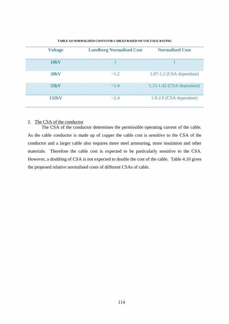
114
TABLE 4.9 NORMALISED COSTS FOR CABLES BASED ON VOLTAGE RATING
Voltage Lundberg Normalised Cost Normalised Cost
10kV 1 1
20kV ~1.2 1.07-1.2 (CSA dependant)
33kV ~1.4 1.15-1.42 (CSA dependant)
132kV ~2.4 1.9-2.0 (CSA dependant)
2. The CSA of the conductor
The CSA of the conductor determines the permissible operating current of the cable.
As the cable conductor is made up of copper the cable cost is sensitive to the CSA of the
conductor and a larger cable also requires more steel armouring, more insulation and other
materials. Therefore the cable cost is expected to be particularly sensitive to the CSA.
However, a doubling of CSA is not expected to double the cost of the cable. Table 4.10 gives
the proposed relative normalised costs of different CSAs of cable.

115
TABLE 4.10 NORMALISED COSTS FOR CABLES BASED ON CSA
CSA (mm2) Lundberg Normalised
Cost
Normalised Cost
35 ~0.8 0.78
50 ~0.85 0.82
70 ~0.92 0.9
95 1 1.0
120 ~1.07 1.1
150 ~1.15 1.2
185 ~1.25 1.3
240 ~1.4 1.5
300 ~1.6 1.8
400 ~1.9 2.1
500 ~2.2 2.5
630 ~2.5 3
3. The installation costs
The installation costs in this case include mobilisation and demobilisation costs,
vessel costs, standby costs, installation of the cable itself, termination and testing of the
cables, onshore installation and termination. These costs can be highly volatile as they are
dependent on vessel availability, location of project, weather conditions during the
installation, proximity of port facilities, seabed conditions, and equipment issues. It can also
be stated that the vessel required will vary for the length and CSA of a given cable to be
installed, and a larger cable presents more difficult handling and installation issues, therefore
making that cable installation more expensive. Longer cables may require jointing between
single lengths which is considered to be factored into the cost.

116
Therefore, with all else being equal on the site, normalised costs for installation are
proposed which are primarily based on the cable CSA. For simplicity, cables are grouped
together in CSA ranges. These are given in Table 4.11.
TABLE 4.11 NORMALISED COSTS FOR CABLES BASED ON INSTALLATION
CSA Range (mm2) Lundberg Normalised
Cost
Normalised Costs
35-70 1 0.8
95-150 1 1
185-300 1 1.2
300+ 1 1.5
Total normalised costs for all submarine cables used in this research is shown in Table
4.12. This is also shown graphically in Figure 4.7. These normalised costs are used for the
economic analysis throughout this section. For comparison the normalised Lundberg cost
model and the normalised cost model developed for this research are shown together in
Figure 4.8.

117
TABLE 4.12 NORMALISED COSTS FOR SUBMARINE CABLES.
Installed Cable Cost
Voltage
Cable CSA (mm2) 10kV 20kV 33kV 132kV
35 0.79 0.82 0.85 1.38
50 0.81 0.85 0.88 1.42
70 0.85 0.89 0.94 1.5
95 1.00 1.05 1.11 1.6
120 1.05 1.11 1.18 1.7
150 1.10 1.17 1.25 1.8
185 1.25 1.34 1.43 1.91
240 1.35 1.46 1.58 2.12
300 1.65 1.80 1.97 2.45
400 1.80 1.99 2.21 2.79
500 2.00 2.25 2.53 3.25
630 2.25 2.55 2.89 3.75
FIGURE 4.7 INSTALLED NORMALISED CABLE COST BY VOLTAGE AND CSA
0.00
0.50
1.00
1.50
2.00
2.50
3.00
3.50
4.00
35 50 70 95 120 150 185 240 300 400 500 630
Inst
alle
d C
able
No
rmal
ise
d C
ost
Cable CSA (mm2)
10kV
20kV
33kV
132kV

118
FIGURE 4.8 COMPARISON OF LUNDBERG MODEL AND RECALIBRATED MODEL
Example:
As outlined in the previous sections, at a normalised cost of 1.0, a 10kV, 95mm2 cable
is the base case for the normalised cable cost model. The following calculation shows what
the difference is between a 33kV, 240mm2 cable and the base case:
Total Normalised Cost = (1*1.5(1)
*(1.1468*1.1373)(2)
) + 1*1.2(3)
)/2
Total Normalised Cost = 1.58
Note:
(1) Difference between 95mm2 and 240mm
2 cable cost
(2) Difference between 10kV 240mm2 and 33kV 240mm
2 cost
(3) Difference between 95mm2
cable installation and 240mm2

119
This shows that a 33kV, 240mm2 cable is 58% more expensive than a 10kV, 95mm
2
cable. Therefore if the installed cost of a 10kV, 95mm2 cable is €350/m then a 33kV,
240mm2 cable costs €553/m.
4.3.13 WEC Array Capacity
No commercial projects are in the latter stages of planning at this time. Therefore, the
‘typical’ rated capacity of a WEC array is uncertain. It is likely that some smaller ‘pre-
commercial’ WEC arrays will be required to provide a bridging market to commercial
projects. By looking at the constraints and the information from the offshore wind industry
the following three stages of development are anticipated.
1. Small scale arrays (pre-commercial demonstrators)
TABLE 4.13 CHARACTERISTICS OF SMALL SCALE ARRAYS
Capacity: 1-10MW
Distance from shore: 10-15km
Transmission voltage: MVAC
Number of transmission connections: 1
2. Medium scale arrays (commercial)
TABLE 4.14 CHARACTERISTICS OF MEDIUM SCALE ARRAYS
Capacity: 10-100MW
Distance from shore: 10-15km
Transmission voltage: MVAC
Number of transmission connections: 2 or more
3. Large scale arrays (commercial)
TABLE 4.15 CHARACTERISTICS OF LARGE SCALE ARRAYS
Capacity: 100MW+
Distance from shore: 15-25km
Transmission voltage: HVAC
Number of transmission connections: 1
For the purposes of this thesis three hypothetical WEC arrays are chosen for detailed
analysis.

120
WEC Array 1 - Small scale array (pre-commercial demonstrator)
TABLE 4.16 CHARACTERISTICS OF WEC ARRAY 1
Capacity: 10MW
Distance from shore: 12km
Transmission voltage: MVAC
Number of transmission connections: 1
WEC Array 2 - Medium scale array (commercial)
TABLE 4.17 CHARACTERISTICS OF WEC ARRAY 2
Capacity: 40MW
Distance from shore: 15km
Transmission voltage: MVAC
Number of transmission connections: 2
WEC Array 3 - Large scale array (commercial)
TABLE 4.18 CHARACTERISTICS OF WEC ARRAY 3
Capacity: 150MW
Distance from shore: 20km
Transmission voltage: HVAC
Number of transmission connections: 1
In the context of this thesis these three WEC array scenarios represent the stages in
the development of WEC arrays. This is a similar development path taken to the
development of large commercial offshore wind farms so it can be reasonably assumed that
WEC arrays will also develop in this manner.
4.4 Key Electrical Interfaces
Before optimising the electrical network configuration the key electrical interfaces
between the array electrical network and the WEC need to be analysed. These key interfaces
are one of the important differences between offshore wind and WEC array electrical
networks outlined in Chapter 3. These key interfaces between the WEC and the electrical

121
network also form part of the overall techno-economic optimisation process, and a balance
between the functionality of these interfaces and cost is required.
These key interfaces are detailed in later sections but are identified as:
1. Dynamic Cable to WEC interface
2. Dynamic Cable to Static Cable interface
3. WEC MV Switchgear interface
4. Offshore Substation
There is a level of functionality required at the key interfaces between the electrical
system and the WECs. In this section these interfaces are considered from the required
functionality within the electrical system. The required functionality includes the following:
Multiple Connection / Disconnection of the WEC
Initial Cable Installation
Electrical Protection
Electrical Isolation (and earthing)
WEC/Cable Hull Penetration
Circuit Continuity (i.e. redundancy)
Various types of WEC will lend themselves better to some of the presented options
than others. The focus here, as already outlined, is on a generic offshore floating WEC array.
Although maximum functionality in the key electrical interfaces would be desirable,
the cost of the key interfaces must also be minimised. Some relative costs are indicated in
these sections based on information from [57] and other various sources. The costs are
indicative only but are expected to be sufficiently accurate for the techno-economic
optimisation undertaken in Section 4.6. The expected costs may limit the functionality that
can be viably achieved in the key interfaces. The balance of cost and functionality is
important and an optimal solution is developed in Section 4.6.

122
4.4.1 Dynamic Cable to WEC Interface
The method by which the dynamic cable is connected to the WEC is of critical
importance to the deployment and retrieval strategy of the WEC array. Some developers
have already considered this, with Pelamis developing a proprietary connection system so the
cable can be connected automatically to the device as it is latched to its moorings [106]. OPT
have developed a floating connection system in cooperation with JDR cables so the cable can
be connected without a diver/ROV to the WEC. It is possible that the main method for
connection / disconnection is to use the submarine connector as detailed in Section 4.4.2.
The system used for the interface between dynamic cable and the WEC should be
simplistic in order to avoid lengthy offshore operations, and flexible in order to allow for
quick connection / disconnection. It should also be noted that for commercial projects the
WECs should ideally remain on station for long periods of time between maintenance so
reliable operation after long periods is required also.
If the system is designed so that the cable can be pre-installed at the site and brought
into the device during deployment, this could allow for the dynamic to static cable connection
to be made during manufacture of the cable, thus reducing the requirement for submarine
cable connectors and hence reducing cost. This is discussed further in the next section.
Some possible dynamic cable to WEC connection schemes are shown for a generic
floating WEC device in Figure 4.9 and the options shown are evaluated.
FIGURE 4.9 DYNAMIC CABLE / WEC INTERFACE OPTIONS FOR WEC

123
(1) Cable routed above the waterline and through a ‘downtube’ to the bottom of the WEC.
The downtube could be internal or external to the WEC hull. A stress reliever would be
required at the bottom of the downtube to avoid stress, kinking or cable damage. If
properly designed this system could allow the cable to be drawn into the device on site
and the cable terminated within the WEC, similar to an offshore wind turbine connection.
This process may be difficult to achieve on a floating WEC. This would mean that when
the cable was disconnected from the device it would need to be capped before it is left
disconnected in situ.
(2) Cable routed directly out through a hull penetration. This would involve a submarine hull
penetration including a stress reliever and seals, in order to maintain hull integrity. This
would mean that the dynamic section of cable would need to be connected during onshore
construction and transported to the site where it would be connected to the static section
of cable already installed.
(3) Cable routed directly out through a hull penetration with a submarine connector. This
would involve a submarine hull penetration including a stress reliever and seals in order
to maintain hull integrity. On the ‘wet’ side of this penetration one half of a submarine
connector would be fixed to the hull. This would mean that the dynamic section of cable,
with the other half of a submarine connector, would need to be connected on site during
installation. This could be by diver, ROV, or an automated system. Pelamis use a system
similar to this for connection of their mooring and power cable simultaneously [106].
Table 4.19 gives indicative relative costs of the various options presented. The
relative costs shown here and in Sections 4.4.2 and 4.4.3 are indicative only, as there is no
available cost information to allow comparison. The least cost option is likely to be (1)
where no hull penetration and sealing is required. Option (2) would require hull penetration
and (3) requires a submarine connector which gives rise to the increase in relative cost.

124
TABLE 4.19 INDICATIVE RELATIVE COSTS FOR WEC TO DYNAMIC CABLE INTERFACE
Option Relative Cost
(1) 1.0 (Base Case)
(2) 1.5
(3) 2.5
4.4.2 Dynamic Cable to Static Cable Interface
The method by which the dynamic cable is connected to the static cable is also of
critical importance to the deployment and retrieval strategy of the WEC array. There are
multiple options for submarine connectors which differ primarily in the ease and speed of
connection, and as a result, cost. Further detailed descriptions are given in Section 3.3.2.
Submarine connectors can be broadly separated into the categories given below.
4.4.2.1 Non-‘Mate-able’ Connector
Permanent/Factory Cable Splice: This is a permanent splice between two cables. This
is the type of splice that is regularly used in factories or in cable repair operations. Once the
splice is made it cannot be separated without cutting the cable. This type of connection can
only be done in very dry and controlled conditions. The cost of these connectors is expected
to be approximately €30,000-40,000 per unit.
4.4.2.2 ‘Mate-able’ Connector
Splice Housing: This is a ‘mate-able’ splice which can be separated and re-connected.
The connector is essentially a housing in which a temporary cable splice can be made. This
type of connection is undertaken on board a service vessel. The cost of these connectors is
expected to be approximately €75,000-100,000 per unit.
Dry-Mate Connector: This is a ‘mate-able’ connector which can be separated and re-
connected numerous times. The dry-mate refers to the fact that this type of connection can
only be undertaken outside of the water on-board a vessel. The cost of these connectors is
expected to be approximately €100,000-150,000.

125
Wet-Mate Connector: This is a ‘mate-able’ connector which can be separated and re-
connected numerous times. The wet-mate refers to the fact that this type of connection can
be undertaken under water on the seabed. The cost of these connectors is expected to be
approximately €200,000-300,000.
The system for interfacing dynamic cable and the static cable should be simplistic in
order to avoid lengthy offshore operations, and flexible in order to allow for multiple quick
connections / disconnections. Some possible dynamic cable to static cable connection
schemes are shown for a generic floating WEC in Figure 4.10.

126
FIGURE 4.10 DYNAMIC / STATIC CABLE CONNECTION OPTIONS FOR WEC
(1) As per option (3) in Figure 4.9, a mate-able connector would be installed at the hull
penetration. This connector would serve a dual purpose as a hull penetration and cable
connector. From the connector the dynamic cable is configured in a lazy-wave to the
seabed where it is connected to the static cable through a permanent/factory splice. The
splice between the static and dynamic cable could be made onshore during cable
manufacture to allow for a simpler installation process. This option however may require
diver, ROV activities, or an automated connection system.
(2) From the WEC standard hull penetration (option (2) in Figure 4.9) the dynamic cable is
configured in a lazy-wave to the seabed where it is connected to the static cable through a

127
mate-able connector such as those outlined in Section 4.4.2. This option could also be
used with option (1) in Figure 4.9 where the cable is routed directly into the WEC on site
without the need for a mate-able connector (the dynamic/static cable interface could be a
permanent splice).
(3) From the WEC a short length (~50m) of dynamic cable is connected to a floatation
module containing a mate-able connector. This floatation module may be part of the
WEC mooring system if a clash between cable and mooring line can be avoided. From
the floatation module the dynamic cable is configured in a lazy-wave to the seabed where
it is connected to the static cable through a factory made joint such as that described in
option (1) above. The short length of dynamic cable to connect to the floatation module
would also be pre-installed before deployment.
Table 4.20 gives indicative relative costs of the various options presented. The least
cost option is (1) where the submarine connector forms part of the WEC to dynamic cable
interface and the dynamic to static cable interface is the lowest cost splice connection. Option
(2) would be slightly more expensive depending on the type of ‘mate-able’ connector used.
Option (3) would be the most expensive depending on the connector used.
TABLE 4.20 INDICATIVE RELATIVE COSTS FOR DYNAMIC CABLE TO STATIC CABLE INTERFACE
Option Relative Cost
(1) 1.0 (Base Case)
(2) 1.2 – 2
(3) 1.3 – 2.5
4.4.3 WEC MV Switchgear Interface
In order to connect the WECs in a radial circuit, MV switchgear is required for
protection of the WEC electrical system and cables, and also for isolation purposes. A
similar switchgear arrangement to offshore wind farms is required in a WEC array.

128
If submarine switchgear is employed this can be coupled with a mate-able connector
system. Submarine switchgear systems have been developed by Siemens [107], ABB [108],
GE Vetco Gray [109], MacArtney [110] and OPT [111]. With the exception of MacArtney
and OPT these have been predominantly designed for offshore Oil and Gas applications
where the economics are of a different order of magnitude to offshore energy generation.
Hence they are designed for extreme deep-water operation (>1000m).
Some possible switchgear configuration schemes are shown for a generic floating
WEC device in Figure 4.11.
FIGURE 4.11 SWITCHGEAR OPTIONS FOR FLOATING WEC

129
(1) From the onboard transformer a dynamic cable is connected (optionally with an onboard
MV circuit breaker) to a submarine switchgear unit (‘hub’), which includes a protection
circuit breaker for the WEC electrical system and dynamic cable, and switch disconnects
for isolation of the cable section. In this way all protection and isolation functions are
done within the subsea module, which would contain protection relays also. This has the
advantage of only one dynamic cable being required for connection to the WEC, but has
issues with regard to electrical safety and maintenance of submarine electrical equipment.
Connectors would also be required to be added to the switchgear unit to allow a
connection / disconnection function also.
(2) From the onboard transformer a cable is connected to onboard switchgear, which includes
a protection circuit breaker for the WEC electrical system, and switch disconnects for
isolation of the dynamic and static cable sections. This system would require two
dynamic cables for WECs connected in a radial network.
(3) From the onboard transformer a cable is connected to onboard switchgear, which includes
a protection circuit breaker for the WEC electrical system and dynamic cable, and switch
disconnects for isolation of the cable section. One dynamic cable is connected to a ‘T’
connector on the seabed (submarine connection ‘hub’). This means that only one dynamic
cable is required for devices connected in arrays. However, to isolate the dynamic cable
section, the entire circuit (including all WECs on the radial) must be switched out and
isolated.
Table 4.21 gives indicative relative costs of the various options presented. The least cost
option is (2) where the switchgear is contained within the WEC itself although this requires
two dynamic cables per WEC. Option (3) is the next most expensive due to the requirement
for additional submarine connectors and a submarine ‘T’ connector. Option (1) is considered
the most expensive due to the requirement for additional submarine connectors and
submarine switchgear.

130
TABLE 4.21 INDICATIVE RELATIVE COSTS FOR DYNAMIC CABLE TO STATIC CABLE INTERFACE
Option Relative Cost
(1) 3 – 5
(2) 1.0 (Base Case)
(3) 2 – 3
4.4.4 Offshore Substation
In offshore wind farms, an offshore substation would be required for arrays over
100MW or those located further than 10km from shore, as these are considered the breakeven
points where the cost of the substation is less than the cost of multiple MV connections. Also
important in the consideration of an offshore wind farm is the voltage for connecting to the
grid, which would normally be HV (>100kV) for large generators.
There are at least 20 offshore substations installed on existing offshore wind farms
with further projects in development or construction. These substations are normally
installed in up to 35m water depth. More detail on offshore wind substations can be found in
Chapter 3.
As offshore WEC arrays are likely be located in 100m water depth, although the
required offshore substation ‘topside’ will be identical, the type of foundations typically used
in offshore wind farm substations will not be practical, i.e. monopile, tripod and gravity-base.
Jacket structures have also been used for ‘deep-water’ sites such as in [89]; however this is
still only 45m depth. Much deeper jacket structures have been deployed in the oil and gas
industry so the technology is feasibly, yet potentially adds a large additional cost to the
project. So the choices for an offshore substation in 100m water depth would be the
following:
Deep-water jacket or compliant-tower type structure such as that in use for oil
platforms. This additional cost will change the breakeven point between multiple MV
connections and a single HV connection.
Strategically locating the WEC array in proximity to a <50m water depth location and
locating the offshore substation at a midpoint between the WEC array and the shore

131
Building the substation on a floating platform such as the semi-submersible, tension
leg or spar type structures in use for oil platforms
Locating the offshore substation on the seabed
The choice of substation design will be a matter of cost and feasibility. The
technologies in use for oil platforms are well proven but the economics of O&G is very
different than that for offshore WEC arrays so may prove too expensive for use in this
industry. Locating the offshore substation on the seabed would solve the foundation platform
issue; however, this has only been achieved on a small power scale and also in the O&G
industry. There would be the same access, maintenance, and safety concerns for this
equipment if this was the case. Sites that have a shallow water location in the vicinity could
possibly be utilised but the economics of the longer MV cables may outweigh the benefits of
this approach. Essentially, a cost benefit analysis must be undertaken on this aspect and this
will not be undertaken accurately until such time as a project at this scale is in development.
It is very likely that the cost of the foundation for a deep-water offshore substation
would be significantly higher than that of a foundation in 0-40m water depth. The full cost
would include the construction and installation including potentially expensive deployment
vessels. The topside of the substation would be approximately the same cost, although some
increase in protection may be necessary to deal with wave loading and installation may also
be more expensive. Therefore it is very likely that the breakeven point for an offshore
substation for a WEC array will be higher than 100MW. It is currently difficult to establish
what the exact breakeven point will be as there are numerous variables in a cost model but
detailed financial models of a specific large wave energy project could establish this.
4.4.5 Submarine Hubs and Substations
Other bespoke solutions have been proposed which all fall into a general category of
‘submarine hubs’ utilising star cluster type network configurations. Star clusters are
considered as a potential network configuration in Section 4.5. The proposed submarine hubs
in general collect the generated power from several WECs and condition it for transmission
to shore. These hubs can contain one or all of the below equipment:
Power Electronic Converters
LV & MV Switchgear

132
Power Transformers
Energy Storage Solutions
Battery Chargers and Auxiliary Systems
The hubs may also be completely passive such as the Wavehub (see Section 3.3.3.2.4
for details). In this case they are acting as a junction box for the aggregation of power from
several WECs.
Although these ‘hubs’ are not evaluated in detail here there are several major
challenges that must be overcome in order to make these types of solutions viable. They are
the same challenges that apply to larger submarine offshore substations (Section 4.4.4). These
challenges are outlined here for information only:
Access to complicated equipment such as power electronic converters, digital
protection relays, and battery chargers would be required in the event of even a simple
fault. This operation alone would result in a large operational cost.
There are safety implications from having a point of isolation and earthing in a
location where it can not be verified or secured (locked out). Some detail on this is
provided in Section 3.3.3.
The practicalities of connecting multiple LV and MV cables to a submarine hub are
onerous. This would require multiple expensive mate-able connectors and/or ROV
operations.
The potential construction and installation costs of a submarine hub are very large and
there is little experience here apart from in the oil and gas industry.
There are other, less technically and economically challenging, options for electrical
connection schemes which should be explored first.
4.5 Array Electrical Network Configuration Evaluation
The array network configuration is a major factor in the cost and functionality of the
array electrical network. There are a variety of possible configurations as shown in Figure
4.12. For WEC arrays some proposals have been made for submarine ‘hubs’ which could act

133
as an aggregation point in a star network. These are discussed in Section 4.4.5 and star
cluster networks are analysed in this section.
FIGURE 4.12 POSSIBLE NETWORK CONFIGURATIONS
In order to evaluate the possible configurations a candidate array, WEC array 2, is
selected from Section 4.3.13. This candidate WEC array is evaluated using the alternative
configurations as shown in Figure 4.12 under a number of economic and functional criteria.
- Economic:
o This considers the increase in the cable cost (relative to configuration (A)) by
a change in the configuration. Costs are taken from Section 4.3.12. A
physical grid layout is considered for all electrical configurations to calculate
the cable lengths and hence costs.
- Functional
o Installation: This considers the complexity of the cable laying operation
compared to a simple radial network scenario. Aspects such as the cable
laying duration and complication are considered.

134
o Operation: This considers the effect of the configuration on the operation of
the WEC array, in particular its availability.
o Maintenance: This considers the ease of maintenance of WECs within the
arrays and the loss of energy when WECs are removed from the array.
o Protection: This considers the location of protection equipment and the ease of
installation and maintenance of same.
The following assumptions are made in addition to those given in Section 4.3:
20kV voltage level is considered for all cases in this section.
Each WEC (node) is 1MW in all cases with unity power factor.
For simplicity only 400m inter-WEC spacing is considered here.
A physical grid layout of the devices is assumed to be maintained, with the
exception of the optimised star-cluster layout.
Redundant circuits are assumed to be rated for worst case full load, i.e. they are
100% redundant.
No bespoke equipment such as submarine switchgear is considered at this stage in
the economic calculations.
All switching operations are assumed to be contained within the WEC or in the
onshore substation.
4.5.1 Simple Radial (A)
FIGURE 4.13 SIMPLE RADIAL CONFIGURATION (NUMBERS BELOW INTER-WEC CABLES DENOTE CSA)
As shown in Figure 4.13 this is the simplest configuration, and as outlined in Chapter
3 this has shown to be the most cost effective for offshore wind farms. In the case of the
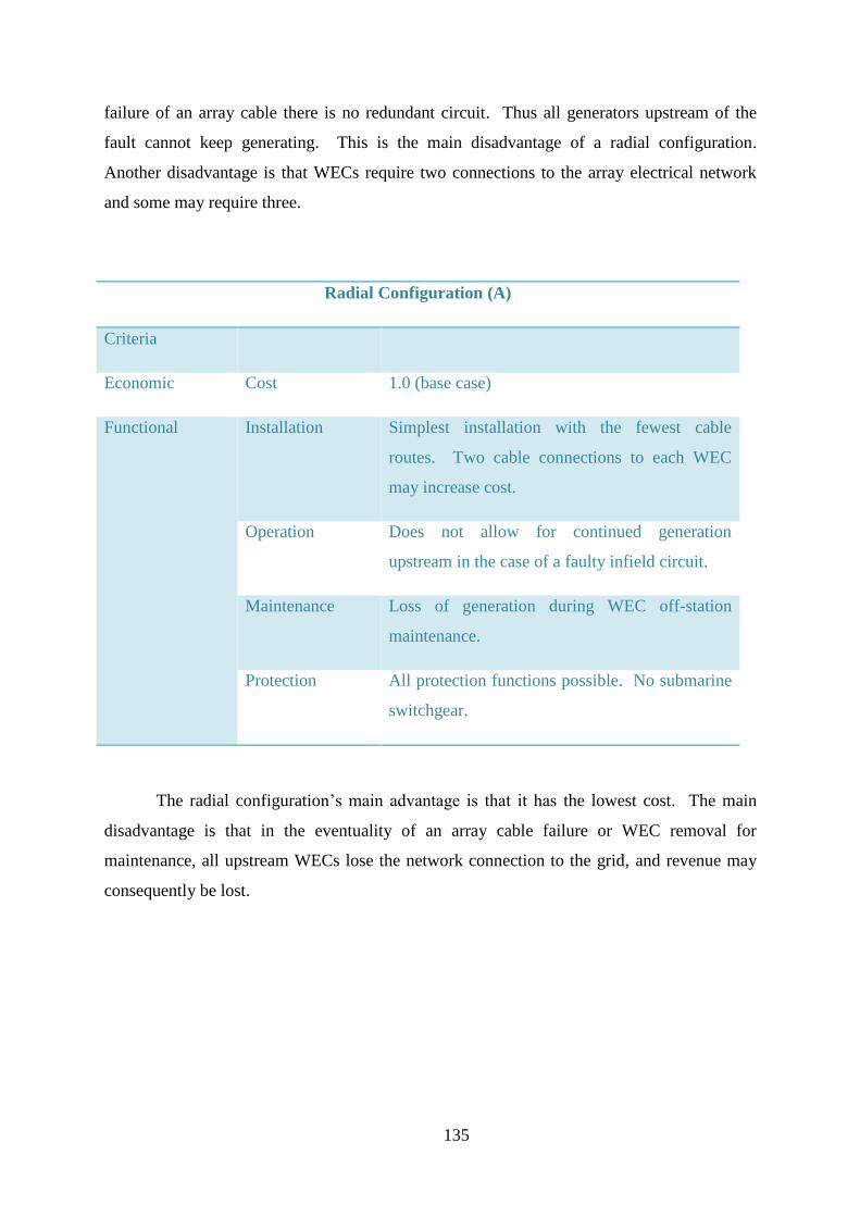
135
failure of an array cable there is no redundant circuit. Thus all generators upstream of the
fault cannot keep generating. This is the main disadvantage of a radial configuration.
Another disadvantage is that WECs require two connections to the array electrical network
and some may require three.
Radial Configuration (A)
Criteria
Economic Cost 1.0 (base case)
Functional Installation Simplest installation with the fewest cable
routes. Two cable connections to each WEC
may increase cost.
Operation Does not allow for continued generation
upstream in the case of a faulty infield circuit.
Maintenance Loss of generation during WEC off-station
maintenance.
Protection All protection functions possible. No submarine
switchgear.
The radial configuration’s main advantage is that it has the lowest cost. The main
disadvantage is that in the eventuality of an array cable failure or WEC removal for
maintenance, all upstream WECs lose the network connection to the grid, and revenue may
consequently be lost.

136
4.5.2 Single Return Ring (B)
FIGURE 4.14 SINGLE RETURN RING CONFIGURATION (NUMBERS BELOW INTER-WEC CABLES DENOTE CSA)
As shown in Figure 4.14 this configuration gives an alternative circuit to shore in the
case of a fault within the array network or the removal of a WEC. Thus all generators can
keep generating once the circuit is reconfigured. The redundant circuit in this case would be
rated to carry the power of one radial. The radial cables’ capacity would need to be increased
to allow for the bi-directionality of this circuit.

137
Single Return Ring Configuration (B)
Criteria
Economic Cost 2.58 x (A)
Functional Installation No more difficult than (A), however it will
require additional time for redundant circuits.
This configuration may influence physical layout
as the array ends may need to be in close
proximity.
Operation Allows for continued generation in the case of a
faulty array or export circuit. Also allows for the
failure of one of the main export cables with
continued (although curtailed) generation.
Maintenance Allows for WEC off-station maintenance with
no loss of generation.
Protection All protection functions possible. No submarine
switchgear.
The single return ring allows the availability of a redundant circuit in case of array or
export cable failure or WEC removal thus overcoming the disadvantage of the simple radial
circuit. This comes at a high cost, as potentially the electrical network cost is 258% of the
cost of the radial configuration.

138
4.5.3 Single Sided Ring (C)
FIGURE 4.15 SINGLE SIDED RING CONFIGURATION (NUMBERS BELOW INTER-WEC CABLES DENOTE CSA)
As shown in Figure 4.15 this configuration gives an alternative circuit for each radial
in the case of a fault of an array cable of WEC removal. This is connected to the beginning
of the radial and not to the shore. Thus all generators can keep generating once the circuit is
reconfigured. The redundant circuit in this case would be rated to carry the power of one
radial. The radial cables’ capacity would need to be increased to allow for the bi-
directionality of this circuit.

139
Single Sided Ring Configuration (C)
Criteria
Economic Cost 1.8 x (A)
Functional Installation May be difficult to accurately run cable circuits
in close proximity to each other. Additional time
will be required for redundant circuits.
Operation Allows for continued generation in the case of a
faulty array circuit or WEC removal.
Maintenance Allows for continued generation in the case of a
faulty array circuit or WEC removal.
Protection All protection functions possible. No submarine
switchgear.
The single sided ring configuration overcomes the disadvantage of the radial
configuration with less additional cost than the single return ring. The cost of this
configuration is still 180% of the radial. There are multiple additional cables required within
the array, which may be difficult to install within an array with small inter device separation.
4.5.4 Double Sided Ring (D)
FIGURE 4.16 DOUBLE SIDED RING CONFIGURATION (NUMBERS BELOW INTER-WEC CABLES DENOTE CSA)

140
As shown in Figure 4.16 this configuration gives an alternative circuit, through the
adjacent radial, for each radial, in the case of a fault within the array circuit or the removal of
a WEC. Thus all generators can keep generating once the circuit is reconfigured. Each radial
in this case would need to be rated to carry the power of two radials in one direction and its
own power in both directions. The radial cables’ capacity would need to be increased to
allow for the bi-directionality and increased capacity of this circuit.
Double Sided Ring Configuration (D)
Criteria
Economic Cost 1.69 x (A)
Functional Installation No more difficult than (A) but will require
additional time for redundant circuits.
Operation Allows for continued generation in the case of a
faulty array cable or WEC removal.
Maintenance Allows for WEC off-station maintenance with
no loss of generation.
Protection All protection functions possible. No submarine
switchgear.
The double sided ring overcomes the disadvantage of the radial configuration for the
least additional cost. The double sided ring still costs 169% of the radial configuration.

141
4.5.5 Star Cluster (E)
FIGURE 4.17 STAR CLUSTER CONFIGURATION (NUMBERS BELOW INTER-WEC CABLES DENOTE CSA)
As shown in Figure 4.17 this configuration gives a separate circuit for almost all
WECs. The exception is the ‘hub’ WECs which could be WECs or simply submarine or
floating hubs/substations. Thus all generators can keep generating if one of the cables to a
WECs fails once there is protection and isolation equipment in the ‘hub’. This also means
that these cables only need to be rated for a single WEC. However, if the same physical grid
layout is maintained some array cables may be relatively long in comparison to radial
network configurations.

142
Star Cluster Configuration (E)
Criteria
Economic Cost 1.54 x (A)
1.06 x (A) when physically optimised – see
below
Functional Installation Could be very difficult to connect multiple
cables to a single WEC or even a single hub.
Cable routes would be complex for vessels to
complete. Cables may have to cross each other.
Operation Allows for continued generation in the case of a
faulty WEC cable. However some cables in the
network would still cause a disconnection of
multiple WECs.
Maintenance Allows for WEC off-station maintenance with
no loss of generation. However if WECs are
used for hubs this may be difficult.
Protection All protection functions possible but hub may
require large amount of switchgear which could
create difficulties. Further issues with
switchgear if submarine hub used.
The star cluster is the least cost option after the radial network, and has a major
benefit of only having a single cable connection to the majority of WECs. The major
disadvantage of the star cluster arrangement is that multiple connections must be made to the
star ‘hub’ which could be a WEC or a submarine/floating ‘hub’. Both of these options could
be difficult to achieve and crucially the system still has a higher cost than a radial
configuration at 154% relative cost.
If the star cluster network is optimised to reduce the length of the connection to the
star ‘hub’ this breaks the physical grid layout of the array but reduce the overall cost of the

143
star cluster network. With nine (9) connections to four hubs (also WECs) and maintaining
the 400m device separation, an optimised star cluster would be almost comparable to a radial
configuration at 106% relative cost. This is illustrated in Figure 4.18.
FIGURE 4.18 ‘OPTIMISED’ STAR CLUSTER CONFIGURATION
4.5.6 Overcoming Radial Limitations
Table 4.22 shows the relative cost of the array only, and the array and export cabling
for the various alternative configurations detailed in Figure 4.12 and the previous sections.
This shows that the radial network is the least cost solution from an array configuration
perspective. This is primarily due to the additional cabling required for the proposed
alternatives. Also to allow redundancy in the circuits the cross sectional area (CSA) of some
of the cables must be increased, thereby also increasing cost.
Spacing
15km 15km
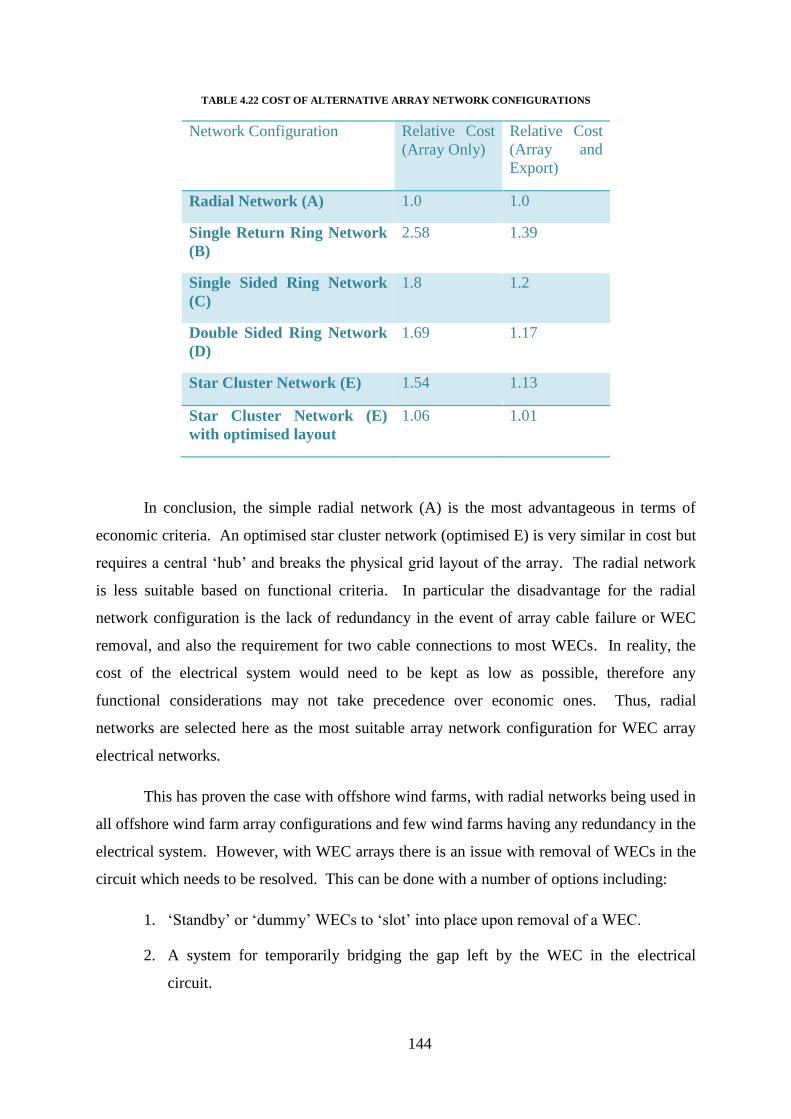
144
TABLE 4.22 COST OF ALTERNATIVE ARRAY NETWORK CONFIGURATIONS
Network Configuration Relative Cost
(Array Only)
Relative Cost
(Array and
Export)
Radial Network (A) 1.0 1.0
Single Return Ring Network
(B)
2.58 1.39
Single Sided Ring Network
(C)
1.8 1.2
Double Sided Ring Network
(D)
1.69 1.17
Star Cluster Network (E) 1.54 1.13
Star Cluster Network (E)
with optimised layout
1.06 1.01
In conclusion, the simple radial network (A) is the most advantageous in terms of
economic criteria. An optimised star cluster network (optimised E) is very similar in cost but
requires a central ‘hub’ and breaks the physical grid layout of the array. The radial network
is less suitable based on functional criteria. In particular the disadvantage for the radial
network configuration is the lack of redundancy in the event of array cable failure or WEC
removal, and also the requirement for two cable connections to most WECs. In reality, the
cost of the electrical system would need to be kept as low as possible, therefore any
functional considerations may not take precedence over economic ones. Thus, radial
networks are selected here as the most suitable array network configuration for WEC array
electrical networks.
This has proven the case with offshore wind farms, with radial networks being used in
all offshore wind farm array configurations and few wind farms having any redundancy in the
electrical system. However, with WEC arrays there is an issue with removal of WECs in the
circuit which needs to be resolved. This can be done with a number of options including:
1. ‘Standby’ or ‘dummy’ WECs to ‘slot’ into place upon removal of a WEC.
2. A system for temporarily bridging the gap left by the WEC in the electrical
circuit.

145
3. Submarine switchgear allowing continued operation of the infield circuit (see
Section 4.4.3).
It is probable that that option 2 here would be the least cost solution to this issue.
For the disadvantage of having two cables connected to most WECs and three to some
the additional cost of this must be more than the additional cost of the star cluster
configuration plus any additional costs inherent in the ‘hub’ required for the star cluster
network. It is possible, but unlikely, that the star cluster configuration would be more
economically competitive than the radial given the higher cost of the network and the
potential hub costs. There are also some methods for overcoming the requirement for two
cables to each WEC such including:
1. The use of submarine switchgear or a passive ‘T’ junction box allowing a single
cable from a radial circuit to the WEC (see Section 4.4.3).
2. The bundling of the two dynamic cables to a single hull penetration into the
device.
3. The bundling of two three-phase cables into a single six core (2 x three phase)
cable through submarine switchgear or a passive ‘T’ junction box.
4.6 Techno-Economic Optimisation
It has been shown in Section 4.5 that a radial array network configuration is the least
cost option for WEC arrays, with the star cluster configuration comparable if the electrical
network design can dictate the physical array layout. The radial configuration, however,
lacks redundancy in the network to cater for WEC removal and a possible requirement for
two cables connected to most WECs. However, solutions are proposed for this in Section
4.5.6. The optimisation of WEC array electrical networks therefore comes through the
selection and design of appropriate interfaces between the WEC and the radial electrical
network. These interfaces must balance cost and functionality.
4.6.1 Least Cost Solution
The least cost solution should involve minimising the use of any potentially expensive
components in the system such as submarine hubs or submarine connectors. Although
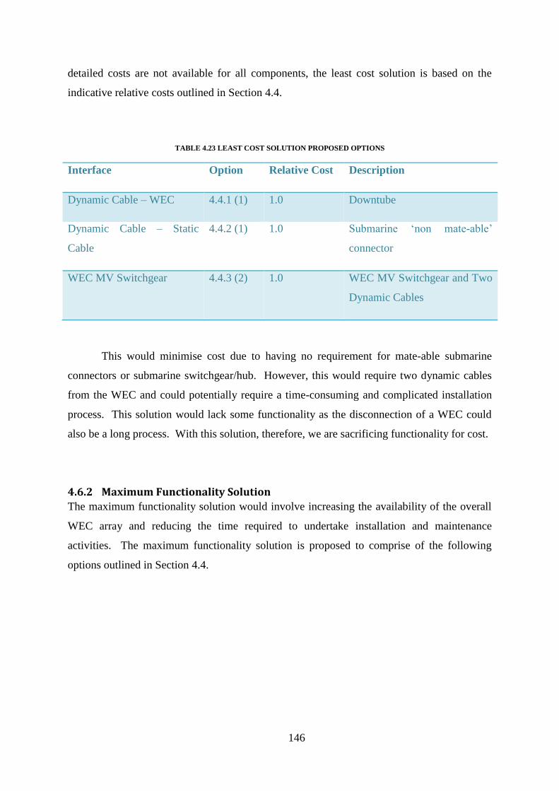
146
detailed costs are not available for all components, the least cost solution is based on the
indicative relative costs outlined in Section 4.4.
TABLE 4.23 LEAST COST SOLUTION PROPOSED OPTIONS
Interface Option Relative Cost Description
Dynamic Cable – WEC 4.4.1 (1) 1.0 Downtube
Dynamic Cable – Static
Cable
4.4.2 (1) 1.0 Submarine ‘non mate-able’
connector
WEC MV Switchgear 4.4.3 (2) 1.0 WEC MV Switchgear and Two
Dynamic Cables
This would minimise cost due to having no requirement for mate-able submarine
connectors or submarine switchgear/hub. However, this would require two dynamic cables
from the WEC and could potentially require a time-consuming and complicated installation
process. This solution would lack some functionality as the disconnection of a WEC could
also be a long process. With this solution, therefore, we are sacrificing functionality for cost.
4.6.2 Maximum Functionality Solution
The maximum functionality solution would involve increasing the availability of the overall
WEC array and reducing the time required to undertake installation and maintenance
activities. The maximum functionality solution is proposed to comprise of the following
options outlined in Section 4.4.

147
TABLE 4.24 MAXIMUM FUNCTIONALITY SOLUTION PROPOSED OPTIONS
Interface Option Relative Cost Description
Dynamic Cable – WEC 4.4.1 (3) 2.5 Hull Penetration /
Connector Combination
Dynamic Cable – Static Cable 4.4.2 (1) 1.0 Submarine ‘non mate-able’
connector
WEC MV Switchgear 4.4.3 (1) 3-5 Submarine MV Switchgear
‘hub’
This solution would allow for easy isolation and removal of the WEC for maintenance
activities while keeping the electrical circuit integrity for upstream devices to continue
generating. Although detailed costs are not available for components, this solution would be
expected to be at least three times the cost of the least cost solution from Section 4.6.1.
4.6.3 Optimised Solution
The optimised solution seeks to maximise functionality at the lowest relative cost. It
is proposed here that circuit continuity (i.e. redundancy) is achieved with a system such as
that proposed in Section 4.5.6. Therefore the only functionality required is to disconnect the
WEC quickly and at the lowest possible cost. The optimised solution is proposed to comprise
of the following options outlined in Section 4.4.
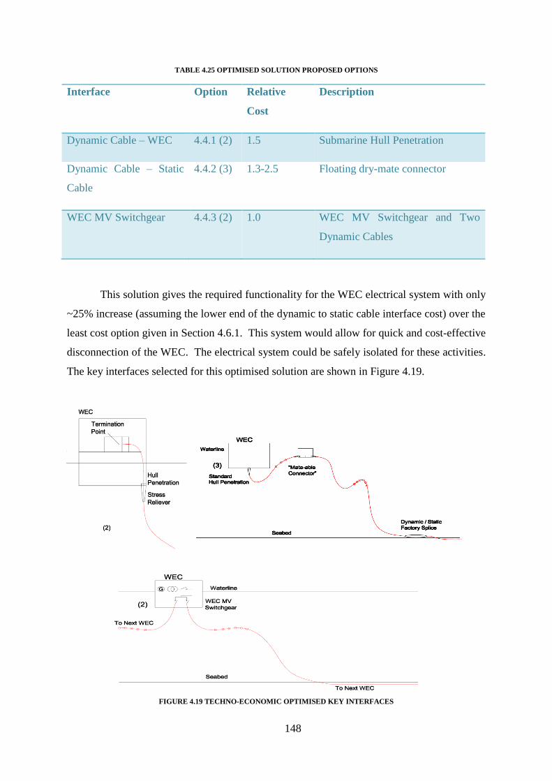
148
TABLE 4.25 OPTIMISED SOLUTION PROPOSED OPTIONS
Interface Option Relative
Cost
Description
Dynamic Cable – WEC 4.4.1 (2) 1.5 Submarine Hull Penetration
Dynamic Cable – Static
Cable
4.4.2 (3) 1.3-2.5 Floating dry-mate connector
WEC MV Switchgear 4.4.3 (2) 1.0 WEC MV Switchgear and Two
Dynamic Cables
This solution gives the required functionality for the WEC electrical system with only
~25% increase (assuming the lower end of the dynamic to static cable interface cost) over the
least cost option given in Section 4.6.1. This system would allow for quick and cost-effective
disconnection of the WEC. The electrical system could be safely isolated for these activities.
The key interfaces selected for this optimised solution are shown in Figure 4.19.
FIGURE 4.19 TECHNO-ECONOMIC OPTIMISED KEY INTERFACES
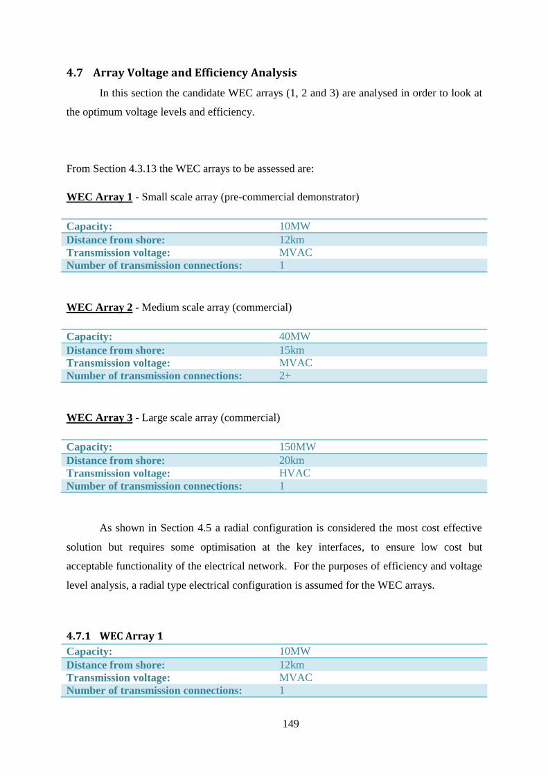
149
4.7 Array Voltage and Efficiency Analysis
In this section the candidate WEC arrays (1, 2 and 3) are analysed in order to look at
the optimum voltage levels and efficiency.
From Section 4.3.13 the WEC arrays to be assessed are:
WEC Array 1 - Small scale array (pre-commercial demonstrator)
Capacity: 10MW
Distance from shore: 12km
Transmission voltage: MVAC
Number of transmission connections: 1
WEC Array 2 - Medium scale array (commercial)
Capacity: 40MW
Distance from shore: 15km
Transmission voltage: MVAC
Number of transmission connections: 2+
WEC Array 3 - Large scale array (commercial)
Capacity: 150MW
Distance from shore: 20km
Transmission voltage: HVAC
Number of transmission connections: 1
As shown in Section 4.5 a radial configuration is considered the most cost effective
solution but requires some optimisation at the key interfaces, to ensure low cost but
acceptable functionality of the electrical network. For the purposes of efficiency and voltage
level analysis, a radial type electrical configuration is assumed for the WEC arrays.
4.7.1 WEC Array 1
Capacity: 10MW
Distance from shore: 12km
Transmission voltage: MVAC
Number of transmission connections: 1

150
The deployment of a 10MW WEC array would most likely be a pre-commercial
demonstrator or early commercial type project in order to prove the deployment of multiple
devices on an array scale. The business case to be made for such a project may be slightly
different to a commercial project due to grant funding and/or a favourable energy tariff.
There would be other aspects of the project where economies of scale would be lost such as
vessel mobilisation and dockside costs. The requirement for high efficiency may not be of
highest priority for this scale of project. High availability may be a more important
consideration.
The electrical configuration in this case is a single radial of ten (10) 1MW WECs.
Figure 4.20 shows the configuration of the 10 devices. If the site configuration permitted, the
main transmission cable could enter the array in the centre (e.g. WEC 6), thus allowing a
tapering of the cable CSA to both sides from this point which would reduce the overall cost
of the cable used within the array.
FIGURE 4.20 WEC ARRAY 1 ELECTRICAL CONFIGURATION
Methodology:
The WEC array electrical network is arranged in radial circuits. For larger arrays a
‘forked’ radial is utilised as this further reduces cable CSA in the radials. The methodology
is as follows:
Cables (array and export) are sized based on maximum continuous current at
10kV, 20kV & 33kV and, for WEC array 3, 132kV. Practical limitations are
observed (see below).
For a given circuit, active power losses are calculated for the range of 0-100% (at
intervals of 10%) wave farm output power for each voltage level using Equation
4.1 and Equation 4.2 given in Section 4.3.9. For clarity these equations calculate
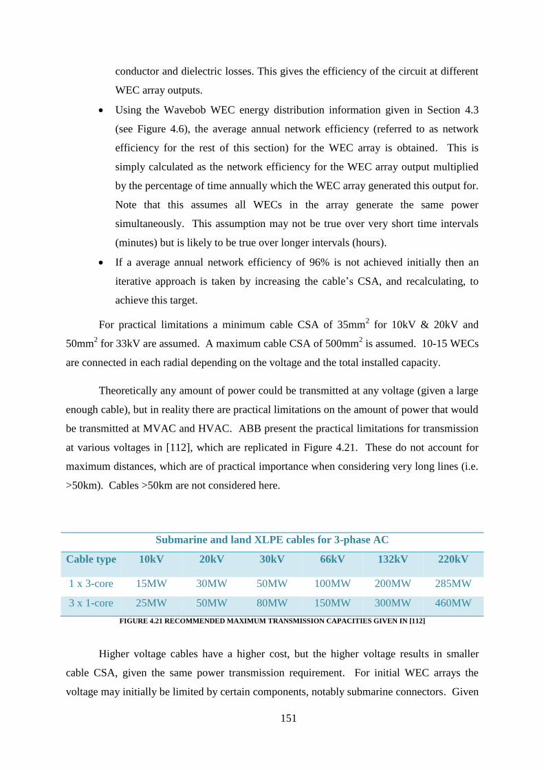
151
conductor and dielectric losses. This gives the efficiency of the circuit at different
WEC array outputs.
Using the Wavebob WEC energy distribution information given in Section 4.3
(see Figure 4.6), the average annual network efficiency (referred to as network
efficiency for the rest of this section) for the WEC array is obtained. This is
simply calculated as the network efficiency for the WEC array output multiplied
by the percentage of time annually which the WEC array generated this output for.
Note that this assumes all WECs in the array generate the same power
simultaneously. This assumption may not be true over very short time intervals
(minutes) but is likely to be true over longer intervals (hours).
If a average annual network efficiency of 96% is not achieved initially then an
iterative approach is taken by increasing the cable’s CSA, and recalculating, to
achieve this target.
For practical limitations a minimum cable CSA of 35mm2 for 10kV & 20kV and
50mm2 for 33kV are assumed. A maximum cable CSA of 500mm
2 is assumed. 10-15 WECs
are connected in each radial depending on the voltage and the total installed capacity.
Theoretically any amount of power could be transmitted at any voltage (given a large
enough cable), but in reality there are practical limitations on the amount of power that would
be transmitted at MVAC and HVAC. ABB present the practical limitations for transmission
at various voltages in [112], which are replicated in Figure 4.21. These do not account for
maximum distances, which are of practical importance when considering very long lines (i.e.
>50km). Cables >50km are not considered here.
Submarine and land XLPE cables for 3-phase AC
Cable type 10kV 20kV 30kV 66kV 132kV 220kV
1 x 3-core 15MW 30MW 50MW 100MW 200MW 285MW
3 x 1-core 25MW 50MW 80MW 150MW 300MW 460MW
FIGURE 4.21 RECOMMENDED MAXIMUM TRANSMISSION CAPACITIES GIVEN IN [112]
Higher voltage cables have a higher cost, but the higher voltage results in smaller
cable CSA, given the same power transmission requirement. For initial WEC arrays the
voltage may initially be limited by certain components, notably submarine connectors. Given

152
the demand, these components would become available at higher voltages; however, it must
be established how cost effective they are.
The cables are sized as outlined in Section 4.3.10 in order to give the optimum
solution for a given voltage level. In this instance 10kV and 20kV are assessed, as the rated
power of the array is considered too low for a 33kV connection. Table 4.26 shows the
detailed cable sizing and loss calculation for the 10MW array, for 200, 300 and 400m device
separation.
Although the device separation is assumed to be 200, 300 and 400m, the cables
lengths examined are 400, 500 and 600m. This is due to the requirement for additional cable
from the seabed into the device. In 100m water depth, an additional 100m at both ends is
assumed.

153
TABLE 4.26 CALCULATION OF LOSSES FOR WEC ARRAY 1 (100% OUTPUT) – 200, 300 & 400M SPACING
The overall network efficiencies for full rated output of the WEC array are given in
Table 4.27.
TABLE 4.27 SUMMARY OF NETWORK EFFICIENCIES FOR FULL RATED OUTPUT
Spacing 200m 300m 400m
Voltage 10kV 20kV 10kV 20kV 10kV 20kV
Efficiency 91.05% 95.10% 90.75% 94.87% 90.45% 94.64%

154
The network efficiency is dependent on the output of the WEC array and will be
higher for lower output power. The network efficiency over the full range of output power is
shown in Figure 4.22 for the 10MW array. It can be seen that the network efficiency of the
10kV network falls rapidly (due to I2R losses) as the WEC array output increases when
compared to the 20kV network.
FIGURE 4.22 EFFICIENCY OF WEC ARRAY 1 VERSUS OVERALL WEC ARRAY OUTPUT
The energy yield distribution of the Wavebob device at the Belmullet site was
determined in Section 4.3.3. Using this, the network efficiency can be calculated.
TABLE 4.28 SUMMARY OF ANNUAL NETWORK EFFICIENCY
Spacing 200m 300m 400m
Voltage 10kV 20kV 10kV 20kV 10kV 20kV
Network
Efficiency
96.21% 97.92% 96.08% 97.82% 95.95% 97.72%
10MW Array Efficiency
90.00%
91.00%
92.00%
93.00%
94.00%
95.00%
96.00%
97.00%
98.00%
99.00%
100.00%
0.00% 20.00% 40.00% 60.00% 80.00% 100.00%
Array Output (%)
Eff
icie
nc
y (
%)
10kV - 200m
20kV - 200m
10kV - 300m
20kV - 300m
10kV - 400m
20kV - 400m

155
This means that, although on initial inspection there would appear to be a 4%
difference in efficiency between a 10kV and 20kV system efficiency, the ‘real’ effect of this
is around 2% difference in annual average network efficiency. This illustrates the importance
of understanding the characteristics of the WEC to establish the true network efficiency.
It also means that, although both 10kV and 20kV initially appear not to have achieved
the 96% efficiency target set out in Section 4.3.7, once the energy distribution of the site and
WEC system is taken into account, the network efficiency is approximately 96% for the
10kV system and over 97.5% for the 20kV system.
From Figure 4.22 it appears that the spacing has minimal impact on the network
efficiency. In fact, from 200 to 400m spacing the difference in network efficiency is 0.26%
for 10kV and 0.2% for 20kV. Spacing would appear not to be critical in the network
efficiency calculation.
Therefore 96% network efficiency can be achieved using the circuit in Figure 4.23
and the cable sizes in Table 4.29.
FIGURE 4.23 WEC ARRAY 1
TABLE 4.29 CABLE CSA (MM2) REQUIRED TO ACHIEVE NETWORK EFFICIENCY OF 96%.
Circuit Section
Voltage 1-2 2-3 3-4 4-5 5-6 6-7 7-8 8-9 9-10 10-Shore
10kV 35 35 70 95 120 185 240 300 300 400
20kV 35 35 35 35 50 50 70 95 95 185
As would be expected the 20kV network requires significantly smaller CSA cables
and this also results in approximately 1.5-2% improvement in energy efficiency over the
10kV system. Using the normalised cable cost model from Section 4.3.12, the relative cost
difference between the 10kV and 20kV network is calculated. In this case, the 20kV system
has a relative cost which is 79% of the 10kV system. Therefore, although the same CSA
cable would be more expensive for 20kV than 10kV, the 20kV network is less costly in this

156
instance as the CSA required for the array and export network is smaller. In this case then
the more efficient operating voltage (20kV) results in a lower relative cost. This does not
consider other component costs such as transformers, switchgear or submarine connectors
which may be more expensive given a 20kV system.
4.7.2 WEC Array 2
Capacity: 40MW
Distance from shore: 15km
Transmission voltage: MVAC
Number of transmission connections: 2+
The deployment of a 40MW WEC array would be a commercial project using proven
WECs on an array scale. The business case to be made for such a project may be helped due
to a favourable, but sustainable, energy tariff. At this size of array, economies of scale would
be possible on common costs. The requirement for high efficiency would be critical at this
point for a viable business case.
The electrical configuration in this case would be four (4) radials of ten (10) 1MVA
WECs. The radials would be connected together at the nearest WEC to shore, and then two
cables would connect the array to the grid. Figure 4.24 shows the configuration of the 40
devices.
FIGURE 4.24 WEC ARRAY 2 ELECTRICAL CONFIGURATION
The cables are sized as outlined in Section 4.3.10 in order to give the optimum
solution for a given voltage level. In this instance 20kV and 33kV are assessed, as the rated
power of the array is considered too high for a practical 10kV network, particularly for

157
transmission to shore. Table 4.30 shows the detailed cable sizing and loss calculation for the
40MW array, for 200, 300 and 400m device separation. Only one half of the array is
assessed (WECs 1-20) but since the other half of the array is a mirror the overall network
efficiency is identical.
TABLE 4.30 CALCULATION OF LOSSES FOR WEC ARRAY 2 (100% OUTPUT) – 200, 300 & 400M SPACING
The overall network efficiencies for full rated output of the WEC array are given in
Table 4.31.

158
TABLE 4.31 SUMMARY OF NETWORK EFFICIENCIES FOR FULL RATED OUTPUT
Spacing 200m 300m 400m
Voltage 20kV 33kV 20kV 33kV 20kV 33kV
Efficiency 94.66% 95.23% 94.52% 95.16% 94.38% 95.08%
The network efficiency is dependent on the output of the WEC array and will be
higher for lower output power. The network efficiency over the full range of output power is
shown in Figure 4.25 for the 40MW array. It can be seen that the network efficiency of the
20kV network is very similar to the 33kV array.
FIGURE 4.25 EFFICIENCY OF WEC ARRAY 2 VERSUS OVERALL WEC ARRAY OUTPUT
The energy yield distribution of the Wavebob device at the Belmullet site was
determined in Section 4.3.3. Using this, the network efficiency can be calculated.
TABLE 4.32 SUMMARY OF NETWORK EFFICIENCY.
Spacing 200m 300m 400m
Voltage 20kV 33kV 20kV 33kV 20kV 33kV
Network
Efficiency
97.73% 97.97% 97.67% 97.94% 97.61% 97.91%
40MW Array Efficiency
94.00%
95.00%
96.00%
97.00%
98.00%
99.00%
100.00%
0.00% 20.00% 40.00% 60.00% 80.00% 100.00%
Array Output (%)
Eff
icie
nc
y (
%)
20kV - 200m
33kV - 200m
20kV - 300m
33kV - 300m
20kV - 400m
33kV - 400m
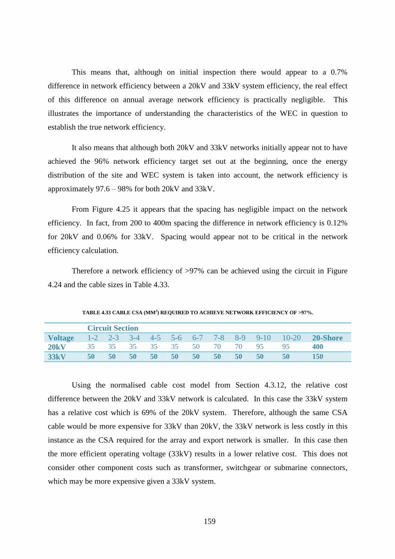
159
This means that, although on initial inspection there would appear to a 0.7%
difference in network efficiency between a 20kV and 33kV system efficiency, the real effect
of this difference on annual average network efficiency is practically negligible. This
illustrates the importance of understanding the characteristics of the WEC in question to
establish the true network efficiency.
It also means that although both 20kV and 33kV networks initially appear not to have
achieved the 96% network efficiency target set out at the beginning, once the energy
distribution of the site and WEC system is taken into account, the network efficiency is
approximately 97.6 – 98% for both 20kV and 33kV.
From Figure 4.25 it appears that the spacing has negligible impact on the network
efficiency. In fact, from 200 to 400m spacing the difference in network efficiency is 0.12%
for 20kV and 0.06% for 33kV. Spacing would appear not to be critical in the network
efficiency calculation.
Therefore a network efficiency of >97% can be achieved using the circuit in Figure
4.24 and the cable sizes in Table 4.33.
TABLE 4.33 CABLE CSA (MM2) REQUIRED TO ACHIEVE NETWORK EFFICIENCY OF >97%.
Circuit Section
Voltage 1-2 2-3 3-4 4-5 5-6 6-7 7-8 8-9 9-10 10-20 20-Shore
20kV 35 35 35 35 35 50 70 70 95 95 400
33kV 50 50 50 50 50 50 50 50 50 50 150
Using the normalised cable cost model from Section 4.3.12, the relative cost
difference between the 20kV and 33kV network is calculated. In this case the 33kV system
has a relative cost which is 69% of the 20kV system. Therefore, although the same CSA
cable would be more expensive for 33kV than 20kV, the 33kV network is less costly in this
instance as the CSA required for the array and export network is smaller. In this case then
the more efficient operating voltage (33kV) results in a lower relative cost. This does not
consider other component costs such as transformer, switchgear or submarine connectors,
which may be more expensive given a 33kV system.

160
4.7.3 WEC Array 3
Capacity: 150MW
Distance from shore: 20km
Transmission voltage: HVAC
Number of transmission connections: 1
The deployment of a 150MW array would be a major commercial project using
proven WECs on an array scale. The business case to be made for such a project may be
helped due to a sustainable energy tariff. At this size of array economies of scale would be
possible on common costs. The requirement for high efficiency would be critical at this point
for a viable business case.
The electrical configuration in this case would be ten (10) radials of fifteen (15)
1MVA devices. The radials would be connected together in pairs at the nearest device to
shore and then five (5) cables would connect the array an offshore substation. As discussed
previously the breakeven point for the use of an offshore substation (versus multiple MV
export connections) in the offshore wind industry is around 100MW. It is expected that this
breakeven point would be higher for WEC arrays but this is dependent on the design of
offshore substations for deep water. 150MW is assumed here to be the point where a deep-
water offshore substation would be economically viable, however it is possible that this
would be higher. The offshore substation aggregates the collected power from all the radials
and steps the voltage up to HVAC for export. Figure 4.26 shows the configuration of the 150
devices. The distance from the offshore substation to the outlying radials is assumed to be 4
times the spacing distance, 2 times the spacing for the next closest radials, and 1 times for the
closest radial.

161
FIGURE 4.26 WEC ARRAY 3 ELECTRICAL CONFIGURATION
The cables are sized as outlined in Section 4.3.10 in order to give the optimum
solution for a given voltage level. In this instance 20kV and 33kV are assessed for the array
circuits, as the rated power of the circuits is considered too high for a practical 10kV network.
The voltage for the transmission to shore is assessed as 132kV, being a typical transmission
voltage used in offshore wind farms. Table 4.34 shows the detailed cable sizing and loss
calculation for the 150MW array, for 200, 300 and 400m device separation.

162
TABLE 4.34 CALCULATION OF LOSSES FOR WEC ARRAY 3 (100% OUTPUT) – 200, 300 & 400M SPACING
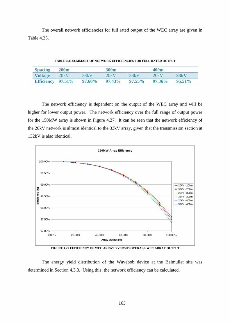
163
The overall network efficiencies for full rated output of the WEC array are given in
Table 4.35.
TABLE 4.35 SUMMARY OF NETWORK EFFICIENCIES FOR FULL RATED OUTPUT
Spacing 200m 300m 400m
Voltage 20kV 33kV 20kV 33kV 20kV 33kV
Efficiency 97.51% 97.60% 97.43% 97.55% 97.36% 95.51%
The network efficiency is dependent on the output of the WEC array and will be
higher for lower output power. The network efficiency over the full range of output power
for the 150MW array is shown in Figure 4.27. It can be seen that the network efficiency of
the 20kV network is almost identical to the 33kV array, given that the transmission section at
132kV is also identical.
FIGURE 4.27 EFFICIENCY OF WEC ARRAY 3 VERSUS OVERALL WEC ARRAY OUTPUT
The energy yield distribution of the Wavebob device at the Belmullet site was
determined in Section 4.3.3. Using this, the network efficiency can be calculated.
150MW Array Efficiency
97.00%
97.50%
98.00%
98.50%
99.00%
99.50%
100.00%
0.00% 20.00% 40.00% 60.00% 80.00% 100.00%
Array Output (%)
Eff
icie
nc
y (
%)
20kV - 200m
33kV - 200m
20kV - 300m
33kV - 300m
20kV - 400m
33kV - 400m

164
TABLE 4.36 SUMMARY OF NETWORK EFFICIENCY.
Spacing 200m 300m 400m
Voltage 20kV 33kV 20kV 33kV 20kV 33kV
Network
Efficiency
98.91% 98.95% 98.87% 98.93% 98.84% 98.91%
This shows that once the energy distribution of the site and WEC system is taken into
account the network efficiency is approximately 98.81 – 98.95% for both 20kV and 33kV
array network and the 132kV transmission network.
From Figure 4.27 it appears that the spacing has negligible impact on the network
efficiency. In fact, from 200 to 400m spacing the difference in network efficiency is 0.11%
for 20kV and 0.04% for 33kV. Spacing would appear not to be critical in the network
efficiency calculation.
Therefore network efficiency of >98.8% can be achieved using the circuit in Figure
4.26 and the cable sizes in Table 4.37.
TABLE 4.37 CABLE CSA (MM2) REQUIRED TO ACHIEVE NETWORK EFFICIENCY OF >98.8% (* 132KV CABLE FOR
TRANSMISSION)
Circuit Section
Voltage 1-2 2-3 3-4 4-5 5-6 6-7 7-8 8-9 9-10
20kV 35 35 35 35 35 50 70 70 95
33kV 50 50 50 50 50 50 50 50 50
Circuit Section
Voltage 10-11 11-12 12-13 13-14 14-15 15-30 30-OSS OSS-Shore*
20kV 120 120 150 185 185 240 2 x 240 500
33kV 50 50 70 70 95 95 300 500
Using the normalised cable cost model from Section 4.3.12, the relative cost
difference between the 20kV and 33kV network is calculated. In this case the 33kV system
has a relative cost which is 95% of the 20kV system. Therefore, although the same CSA
cable would be more expensive for 33kV than 20kV, the 33kV network is less costly in this
instance as the CSA required for the array and export network is smaller. In this case then,
the marginally more efficient operating voltage (33kV) results in a lower relative cost. This
does not consider other component costs such as transformers, switchgear or submarine
connectors which may be more expensive given a 33kV system.

165
4.7.4 Summary
The results are summarised in Figure 4.28 showing the achievable network efficiency
for the candidate WEC arrays 1, 2 and 3 presented in this section. It is important to note that
these network efficiencies are achievable for the generation characteristic introduced in
Section 4.3.3. However, it is also important to note that the real network efficiency for an
electrical network cannot be calculated without an understanding of the generation
characteristic of the WEC devices.
FIGURE 4.28 ACHIEVABLE NETWORK EFFICIENCY FOR WEC ARRAYS 1-3
Also of note from Figure 4.28 is that array spacing has negligible impact on the
network efficiency of the WEC array electrical network. However, as shown in Figure 4.29,
increased array spacing increases the length of cable required within the array and this has an
impact on the economics of the WEC array electrical network. This is explored further in
Chapter 5.

166
FIGURE 4.29 INCREASE IN ARRAY CABLE LENGTH FROM INCREASED SPACING.
4.8 Achieving CAPEX Targets
In this chapter, a techno-economic optimisation exercise has been carried out in order
to assess the best technical solution that can be achieved within the target costs of €1m/MW
as introduced in Section 4.2. However, normalised (or relative) and indicative costs have
been used. This acknowledges that actual costs are difficult to quantify in a generic sense
and are also volatile over time. The following costs are assumed for the cable and key
interface components in WEC array 2, the 40MW array.
Base case cable cost (10kV, 95mm2) of €350/m installed
Base case cost for key interfaces:
1. Dynamic Cable to WEC: €100k
2. Dynamic Cable to Static Cable: €40k
3. WEC MV Switchgear: €0k (included in WEC cost)
4. Offshore Substation: N/A
Using the above estimated base cost, the total cost for WEC array 2 electrical network
is shown in Table 4.24. Note that 400m array spacing and 33kV voltage are assumed.
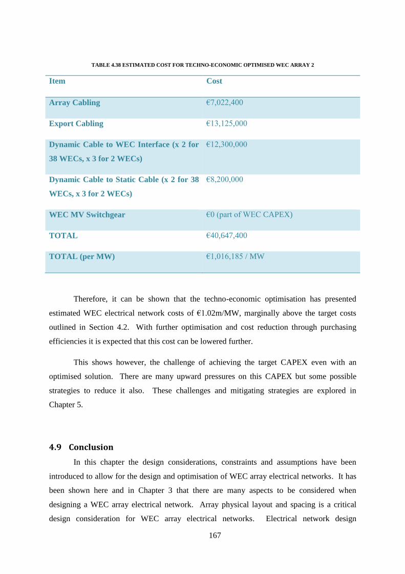
167
TABLE 4.38 ESTIMATED COST FOR TECHNO-ECONOMIC OPTIMISED WEC ARRAY 2
Item Cost
Array Cabling €7,022,400
Export Cabling €13,125,000
Dynamic Cable to WEC Interface (x 2 for
38 WECs, x 3 for 2 WECs)
€12,300,000
Dynamic Cable to Static Cable (x 2 for 38
WECs, x 3 for 2 WECs)
€8,200,000
WEC MV Switchgear €0 (part of WEC CAPEX)
TOTAL €40,647,400
TOTAL (per MW) €1,016,185 / MW
Therefore, it can be shown that the techno-economic optimisation has presented
estimated WEC electrical network costs of €1.02m/MW, marginally above the target costs
outlined in Section 4.2. With further optimisation and cost reduction through purchasing
efficiencies it is expected that this cost can be lowered further.
This shows however, the challenge of achieving the target CAPEX even with an
optimised solution. There are many upward pressures on this CAPEX but some possible
strategies to reduce it also. These challenges and mitigating strategies are explored in
Chapter 5.
4.9 Conclusion
In this chapter the design considerations, constraints and assumptions have been
introduced to allow for the design and optimisation of WEC array electrical networks. It has
been shown here and in Chapter 3 that there are many aspects to be considered when
designing a WEC array electrical network. Array physical layout and spacing is a critical
design consideration for WEC array electrical networks. Electrical network design

168
economics is just one consideration for the physical layout and spacing, and any implications
on criteria such as interference, moorings or vessel access must be considered.
From the analysis in Chapter 3 the key differences between offshore wind electrical
networks and WEC array electrical networks have been identified. In particular the key
interfaces of the WEC array electrical network have been introduced and analysed. These
key interfaces are critical to the functionality of a WEC array electrical network but may be
high cost items. Several alternative designs have been proposed for these key interfaces and
have been assessed for functionality and relative cost.
The array network configuration alternatives have also been assessed from an
economic and functional perspective. It is concluded that the radial network would be the
optimum network as it is likely to be the lowest cost. There are deficiencies with a radial
network for a WEC array, and these have been addressed with some solutions proposed to
overcome these deficiencies.
Star cluster networks overcome these limitations at a comparable cost. There is,
however, a requirement for a collector ‘hub’ within star cluster networks. These hubs have
been proposed involving complex power equipment located in submarine hubs on the
seafloor. This is feasible, but presents economic, technical, and safety concerns. Radial
networks may be easier to implement in a more cost effective and safe manner in the
medium-term.
For a radial network a techno-economic optimisation has been undertaken which
defines the least cost key interfaces while maintaining the necessary functionality in the WEC
array electrical network. This optimised solution allows the WEC array electrical network to
be achieved at costs which are within the target envelope for commercial WEC arrays.
Some candidate WEC arrays from 10MW – 150MW have been evaluated to
understand the achievable annual average network efficiency of the WEC array electrical
network. This shows that network efficiencies of >96% and up to 99% can be achieved for
the presented WEC array electrical network designs. Higher voltage ratings increase network
efficiency and result in lower cable cost but this may be negated by higher cost transformers,
switchgear and submarine connectors. Increased spacing has negligible effects on network
efficiency but has an economic penalty as will be discussed in Chapter 5.

169
The optimised electrical network has been shown to be achievable within the
presented target costs for the electrical networks for commercial WEC arrays, i.e. €1m/MW

170

171
5 Economic Challenges and Cost Reduction Strategies for WEC Array Electrical Networks
Chapter 5
Economic Challenges and Cost
Reduction Strategies for WEC Array
Electrical Networks
5.1 Introduction
In this chapter economic challenges, unique to wave energy electrical network design,
are introduced. These challenges are analysed to quantify the impact of design decisions on
the techno-economic performance of WEC array electrical networks. The optimised array
network which is outlined in Chapter 4 is used as a candidate in analysis.
There are also potential strategies to improve the economics of the WEC array
electrical network. The strategies for maximising the value of the WEC array electrical
network are introduced and evaluated for the optimised candidate network.
5.2 Economic Challenges for WEC Array Electrical Networks
As there is likely to be significant pressure on the overall business case for early stage
WEC arrays, it is necessary to reduce the costs of major capital expenditure such as the
electrical network. However, designers must be wary not to compromise critical safety and
functionality in order to meet this downward cost pressure.
The ‘medium’ size, 40MW, WEC array is taken from Section 4.7.2 as a candidate
array. This is shown in Figure 5.1. This candidate array has the following assumptions for
analysis in this chapter:
Each WEC (node) is rated at 1MW with unity power factor
Each WEC has a 30% capacity factor

172
The inter-WEC spacing is 400m (array cables are 400m + twice the depth)
The water depth is 100m
The export distance is 15km
Operating voltage is 20kV unless otherwise stated
This is used in conjunction with the normalised cable cost model given in Section
4.3.12 in order for an economic analysis to be undertaken.
FIGURE 5.1 CANDIDATE, 40MW WEC ARRAY 2
5.2.1 Redundancy and Star Cluster Networks AS OUTLINED IN SECTION 4.5, RADIAL NETWORKS RESULT IN THE LOWEST COST BUT LACK REDUNDANCY.
REDUNDANCY. REDUNDANCY CAN BE ADDED TO THE NETWORK CONFIGURATION BUT AT A COST. IN SECTION
4.5 THIS COST IS QUANTIFIED FOR VARIOUS NETWORK CONFIGURATIONS WITH THE RELATIVE COSTS GIVEN IN
Table 4.22.
Star cluster networks may be attractive, as when they are physically optimised, they
can have costs similar to radial networks. There are additional challenges associated with the
necessary ‘hubs’ in star cluster configurations. These challenges may increase costs of the
array electrical network substantially. This is detailed in Section 4.4.5. Ultimately, WEC
array electrical network designs which utilise star cluster networks with submarine ‘hubs’
may not achieve target costs.

173
5.2.2 WEC Array Spacing
In Section 4.7.4 the potential additional cost of increasing WEC spacing from 200m
to 400m is introduced. This shows that, for certain arrays, doubling the spacing from 200m
to 400m could increase the circuit length (and hence costs) by up to 37% (see Figure 4.29).
There is a balance between optimizing the array spacing for hydrodynamic
interference and also reducing the electrical system costs. The increased cost associated with
increasing array spacing must be offset by the resultant potential increased yield or lower
losses though interference.
5.2.3 Individual WEC ratings
At the current stage of the industry’s maturity there is a trend, both in the wave and
tidal sectors, towards devices with ratings of 1MW. Individual WEC ratings of 1MW are
therefore used as the base case in any analysis done in this thesis. There are, however, a
number of exceptions to this trend. Offshore wind turbines are mostly rated around 3-4MW
with a trend towards higher power turbines (5MW and larger). These smaller device ratings
present a challenge to the economics of WEC array electrical systems as each device in an
array requires dynamic cables (floating WEC), submarine connectors, and a cable connection
to the next device in the array. More devices in the array means additional cost for the array,
certainly on a per MW level.
The costs of the dynamic and static submarine cables only is evaluated here, as the
export cable cost would not change given the same array rating. The relative cost of the array
electrical network (versus the base case) is established for a 40MW WEC array with 250kW,
500kW, 1MW (base case), 2MW, and 4MW individual WEC ratings. The overall rating of
the array remains at 40MW in all cases, i.e. the quantity of WECs changes depending on the
WEC rating. Therefore, for 250kW WECs there are 160 WECs in the array, for 500kW there
are 80 WECs, for 2MW there are 20 WECs, for 3MW there are 13 WECs, and for 4MW
there are 10 WECs. The array and export voltage is also 20kV in all cases.
As lower rated WECs are likely to require less spacing between devices, the array
spacing is adjusted using a scaling factor (approximate Froude scaling). Therefore, for
250kW WEC spacing is 268m, for 500kW spacing is 328m, for 2MW spacing is 480m, for
3MW spacing is 544m, and for 4MW spacing is 592m.

174
The relative cost as a multiple of the base case is calculated by re-assessing the cable
CSA requirements for the array network in each case, and calculating the relative cost using
the normalised submarine cable cost model (Section 4.3.12). The results are shown in Figure
5.2. The relative cost is shown for the array electrical network only and the full electrical
system (i.e. array and 15km export cable). This shows that the relative cost of the array
electrical network is higher given smaller WECs in the network and lower given larger
WECs. The increase can be as much as 3 times for the array cable costs. It should be noted
that the costs do not decrease as significantly for larger individual WECs, with decreases to
as low as 0.4 times possible for the array cable costs.
FIGURE 5.2 RELATIVE COST OF 40MW ARRAY ELECTRICAL CABLING BASED ON DEVICE RATING
The focus here is on the electrical network cables only. However, it is worth noting
that lower WEC ratings increase other elements of CAPEX such as installation and moorings.
5.2.4 Device Capacity Factor
The capacity factor of offshore wind turbines is typically in the region of 30-40% [71]
depending on turbine type, location, and yearly wind speed. Given the variety of WEC

175
concepts available, it is unclear what capacity factors these WECs will have. For ‘direct
drive’ WECs, the capacity factor could be very low; <20%, due to the need for a high peak
power rating (relative to the average) to absorb wave energy.
The relative cost of the array electrical network (versus the base case) is established
for the candidate array with capacity factors of 10%, 20%, 30% (base case), 40%, 50% and
60%. In order to allow a comparative analysis, the annual energy from the array remains
constant. Therefore, the average output of the array remains at 12MW (base case 40MW x
30%) in all cases but the peak power output changes with the capacity factor. E.g. an array
with 10% capacity factor has a peak output of 120MW but an average output of 12MW.
The relative cost as a multiple of the base case is calculated by re-assessing the cable
CSA requirements for the array network in each case, and calculating the relative cost using
the normalised submarine cable cost mode (Section 4.3.12). The results are shown in Figure
5.3. The relative cost is shown for the full electrical network only (i.e. array and 15km export
cable). This is because capacity factor affects the cost of both array and export systems. The
relative cost is assessed at two voltage levels (20kV and 33kV). This shows that the relative
cost of the electrical network is higher for WECs with lower capacity factor, and lower for
WECs with higher capacity factor. Halving the capacity factor from 30% to 15% would
almost double the cost of the electrical network. Doubling the capacity factor from 30% to
60% would decrease the costs by up to 40%.
FIGURE 5.3 RELATIVE COST OF 40 DEVICE ARRAY ELECTRICAL CABLING BASED ON DEVICE CAPACITY FACTOR

176
5.2.5 Submarine Connectors and other Submarine Electrical Systems
In offshore wind farms the cables are routed, through J-tubes, straight into the turbine
tower. This is not the case with WEC arrays as the devices are required to be removed for
maintenance on a regular basis. This presents a number of issues including redundancy in the
electrical network, which is discussed in Section 4.5. For floating WECs, there is a
connection required between the dynamic cable and the static cable. In some cases there is a
requirement for the device to be quickly and repeatedly connected and disconnected from the
electrical network, although more so at prototype stage. Therefore, some type of connector is
required. These connectors are discussed in Sections 3.3 and 4.4.
However, as these connectors are a requirement for WEC array electrical networks,
which does not exist in offshore wind, they add to the overall cost of the electrical network.
In some cases, where a radial circuit is used, there is a requirement for two connectors per
device. As mentioned in Section 4.2, the electrical network has a target cost of €1m/MW.
Also. Section 4.4.2 shows that electrical connectors could cost anywhere from €30-€300k
per installed connector. To avoid exceeding the threshold of €1m/MW two €250k connectors
may not be feasible, i.e. €0.5m/WEC on connectors alone. If the individual WECs are larger
than 1MW this may help to reduce the ‘per MW’ cost of the submarine connectors.
Although wet-mate connectors may increase the functionality of the device, they may
be unfeasible in the medium-term due to cost. Ultimately, submarine connectors are required
and it is simply a matter of trying to balance the cost with the functionality of the connector.
This has been discussed in Section 4.6.
5.2.6 Array and Export Voltage
The voltage of the array and export system is an important design factor when
considering the cost of the electrical network. The array voltage can be dictated by the WEC
design or the availability of key interface components such as submarine connectors. It is
desirable for the array and export system voltage to be as high as possible, but this is
constrained by economic considerations and component availability.
Typical offshore wind farm array systems operate at 33kV [64], with a move towards
array systems at up to 66kV. Typically the array system is connected in multiple radials to a

177
fixed offshore substation where the voltage is stepped up to high voltage (132kV+) for export
to shore. For WEC arrays it is likely that lower voltages will be used initially due to the
rating of individual WECs and limited array sizes. Eventually, voltages of up to at least
33kV will be required for WEC arrays although array voltages may need to be higher to
avoid the complications of offshore substations in deeper water as outlined in Section 3.3.4.
It is difficult to quantify a generic cost difference for various array and export
voltages, as each WEC array will have different considerations depending on a variety of
factors including number of WECs, WEC ratings, array spacing, distance to shore, and grid
connection voltage. Although increasing the voltage rating of a particular cable increases the
cost of that cable (if the cross sectional area (CSA) remains the same), an increased voltage
rating allows a lower current rating and hence a smaller CSA. Therefore, in certain
circumstances, and notably for larger arrays, an increase in voltage can ultimately decrease
the electrical network costs, particularly for the cable element of this cost. Increase in
voltage of the network, however, causes an increase in cost of other equipment like
switchgear and transformers.
As an example, the information presented in Figure 5.3 (which shows relative figures
only) is reproduced in Figure 5.4, illustrating the absolute difference in cost between 20kV
and 33kV array and export cable systems for a variety of WEC capacity factors. The cost
difference can be up to 33% for low capacity factors (where high CSA is required at lower
voltages); however, this can reduce to almost 0% difference for 40% capacity factors. For
clarity, this means that the 33kV system can be up to 33% less costly than a 20kV system at
lower capacity factors and is not more costly for our candidate array.
In conclusion, selecting the optimum system voltage can have an impact on the
economics of the electrical system but each array must be evaluated separately.

178
FIGURE 5.4 COST DIFFERENCE BETWEEN 20KV AND 33KV VOLTAGE FOR 40 DEVICE FARM ELECTRICAL CABLING
BY WEC CAPACITY FACTOR
It is also worth noting that increasing the system voltage may have impacts on the key
interfaces such as the submarine connector discussed in Section 5.2.5.
5.2.7 Cable Installation and Export Distance
Seabed characteristics have a significant impact on the cost of submarine cable
installations with the ideal conditions for cable laying and protection being soft mud, sand or
clay where the cable can be ploughed into the sand and buried to a depth where it is protected
(typically 2 metres). Conveniently, this would also be an ideal condition for drag embedment
anchors for WEC mooring. However, not all sites have these conditions, particularly high
energy (wave and tidal) sites that may have little or no sediment cover or mobile sediment
[113]. Cable installations might be required in sites that have swept rock, cobble, reefs,
boulder fields, glacial till, or other characteristics. In some cases the cable route may cross
several distinctly different seabed conditions.
The impact this can have on the economics of the electrical system cannot be
underestimated. Trenching methods requiring rock saws radically increase installation costs.
Post-installation protection using rock dumping or concrete mattresses could cost more than
the installed cable itself and therefore could potentially double the costs [57]. These costs are
not quantified here but the economics of the cable installation and protection forms an
Cost Difference between 20kV and 33kV Voltage for 40 WEC Array
Electrical System by WEC Capacity Factor
0.00%
5.00%
10.00%
15.00%
20.00%
25.00%
30.00%
35.00%
0% 10% 20% 30% 40% 50% 60% 70%
Capacity Factor (%)
Co
st
Dif
fere
nce

179
integral part of the site selection process. Sites which allow lower cost cable installations will
ultimately be more competitive. A number of installed wave and tidal facilities have required
these measures such as:
EMEC (Armour Casings and Concrete Mattresses)
Wavehub (Rock Dumping)
MCT SeaGen (Horizontal Directional Drilling)
Careful selection of sites with sediment is one way of avoiding expensive cable
installation methods. This could go hand in hand with mooring requirements for wave
energy arrays.
There is also a challenge in the protection of dynamic power cables as this requires
numerous additional components such as bend restrictors, stress relievers, floatation module
and scour protection. Again, this adds to the cost of the electrical system. Nevertheless, this
increase is expected to be relatively modest.
Export distance also has a very understandable impact on the cost of the electrical
system. This does not need to be quantified and it should be obvious that longer export
systems, which should be noted to include the offshore distance from the WEC array to the
shore landing as well as the onshore distance to the grid connection point, increases costs.
This should also form an integral part of the site selection process and some sites will benefit
from short export distances and grid connection points close to the cable landing point.
Finally, offshore substations may be cost-prohibitive to install at deep-water WEC
array sites and require expensive foundation solutions such as jacket structures, or
alternatively, semi-submersible, spar or submarine installation. These requirements increase
the cost of an offshore substation dramatically and very large arrays may be required before
such an expense can be justified.
5.2.8 WEC Dynamic Response
As with the site characteristics, the effect of the WEC dynamic response on the
economics can be difficult to quantify as there are many factors which must be considered in
the design of a dynamic cable. The response amplitude operator (RAO) of the device
describes the behaviour of the device in real sea-states. There is no doubt that WECs with a

180
lower dynamic response cause less stress, acceleration and fatigue loading on the cable,
which in turn enable the construction cost of the cable to be lower.
Fatigue lifetime of materials is an important design consideration of dynamic cables
[85] and there are considerations to be made at pinch points of the cable. For example, the
connection to the WEC where a stress reliever is required and the cable accessories including
buoyancy module, vortex induced vibration strakes, and scour protection. All of these
elements add to the cost of the dynamic cable and consequently to the overall electrical
system cost.
It is anticipated that the impact of this on the overall electrical network cost is
relatively limited, although certainly not insignificant.
5.3 Maximising Value from WEC Array Electrical Networks
In this section strategies to reduce the CAPEX of the electrical network of WEC
arrays are introduced, i.e. strategies to maximise the value of the electrical network asset with
particular emphasis on the cabling system. This in turn reduces the overall CAPEX of WEC
arrays and help allow cost competitive wave energy to be realised.
There are a number of strategies explored here in order to achieve this increase in
value from the WEC array electrical network. In some cases, comparison is made to offshore
wind to provide context. However, it should be noted that WEC devices have very different
characteristics than offshore wind turbines.
5.3.1 Strategies for Maximising Value of WEC Array Electrical Networks
5.3.1.1 Addressing Economic Challenges
There are numerous challenges to the economics of WEC array electrical networks
introduced throughout Chapter 4 and in Section 5.2. It is noted that through careful design of
WEC devices and WEC arrays these challenges can be addressed. Optimum design of WEC
devices in terms of device rating, capacity factor, and device response characteristics reduce
the costs for WEC array electrical networks. Costs can also be reduced through optimum

181
design of WEC arrays in terms of array spacing, electrical network configuration, key
interfaces, and site characteristics.
Some of these cost reduction opportunities are outlined in Chapter 4 and in Section
5.2. The sections below describe additional strategies that may allow some reduction in the
costs of WEC array electrical networks.
5.3.1.2 Less Than 100% Rating Based on Statistical Data
It is expected that a WEC Array would reach 100% output for only a small proportion
of its annual operation. This leads to the hypothesis that the electrical export system could be
rated at less than 100% of the ‘nameplate’ rating of the WEC array. In this case the rating
means that the export cable is under-rated when the WECs do reach maximum output
simultaneously, leading to either output curtailment or a combination of one of the techniques
described in Section 5.3.1.3 and 5.3.1.4. However any potential loss in generated energy
revenue may be offset by the savings gained from using a lower rated cable.
The UK National Grid & Crown Estate established the optimum economic case for
electrical export systems for offshore wind farms in [114]. This concluded that the optimum
wind farm capacity is 112% of the export cable capacity, i.e. the optimum export cable
capacity is 89.3% of the wind farm capacity. This finding is based on the optimum
MWh/£GB CAPEX, taking into account availability and overall lifetime economics of the
wind farm. The report acknowledged that curtailment of generation would be necessary at
certain times. The same conclusions may not be true for WEC arrays with different
generation characteristics but this demonstrates the viability of exploring the concept for
wave energy.
By simulating a small WEC array, the effect that <100% rating of the cabling has on
the proportion of time that the cable limits are exceeded can be evaluated. From this, the
effect on the annual energy yield of the array can be established and it can be seen whether
this is offset by the savings in the CAPEX of the electrical network. This analysis is
presented in Section 5.3.2.1.

182
5.3.1.3 Dynamic Rating Based on Environmental Data
The current carrying capacity, or ampacity, of power cables is calculated according to
IEC60287 [98]. The maximum permissible continuous current is based on the maximum
conductor operating temperature as defined by the cable manufacturer. For XLPE insulated
cables this temperature is typically 90°C but can be lower. The cable must dissipate heat
during normal operation so the maximum permissible current is calculated based on the
thermal properties of all of the components of the cable (insulation, screens, sheaths, filler,
armour, and serving), the cable geometry, and the thermal properties of the surroundings.
The current ratings given in submarine cable specifications such as [84] use assumed
values for the ambient conditions and surroundings such as those given below:
Ambient temperature of 20°C
Sheaths bonded at both ends and earthed
Burial depth of 1 metre
Thermal resistivity of surroundings of 1 Km/W
The ambient temperature, burial depth and thermal resistivity of the surroundings are
somewhat within the control of the designer. These vary over time and over the length of the
cable route. Therefore the maximum permissible current similarly varies over time and
across the route.
5.3.1.4 Dynamic Rating Based on Real-Time Measurement
Dynamic or Real Time Thermal Rating (RTTR) systems have been developed in
order to utilise the ‘headroom’ available in transmission assets to increase the capacity at a
given location. These systems monitor the environmental conditions (such as temperature
and humidity) and/or measure/model the temperature of the conductors themselves so as to
allow dynamic constraints to be set on the system. This has been shown to allow 10-30%
increased capacity over the static thermal rating of overhead lines [79].
To date this has been utilised successfully, with varying levels of sophistication, on
transmission systems in a number of countries. It has also been utilised for offshore wind
farm export cables [82].
These measurement technologies ensure that an accurate figure of the cable ampacity
is maintained at all times, thus allowing the cable asset to be utilised to its actual full

183
permissible rating when required. Similar to the methodology in Section 5.3.1.3, this would
give greater accuracy and confidence regarding the actual maximum current rating at any
given time.
5.3.1.5 Other Methods
Other methods which could potentially be employed include gas or liquid cooling,
and burial methods (such as backfilling with low thermal resistivity aggregate), but these are
considered outside the scope of this study as they are expected to be cost prohibitive.
Also of note is the study in [104] which looks at the ‘sharing’ of an export cable
between an offshore wind farm and a WEC array. This is a novel idea and is shown to be
advantageous in [104]; however it is not explored further here.
5.3.2 Detailed Analysis and Results
Below is the detailed analysis performed for the strategies presented above. The
method used is outlined in each section and the analysis is performed on the candidate WEC
array, Figure 5.1, with the exception of 5.3.2.1 which uses a 5 device array to reduce the
complexity of the calculations.
5.3.2.1 Less Than 100% Rating Based on Statistical Data
A small WEC array is examined to assess the possibility of lowering the rating of
some of the cables, thus realising cost savings. For simplicity a 5-WEC array is considered
here. It should be noted that this is a much simplified, idealised model of the system which is
intended to demonstrate the principle only. It is noted that each WEC has a different
characteristic and the potential for this solution must be evaluated on a case by case basis.
Unlike the candidate WEC array (Figure 5.1), the physical spatial arrangement of the
devices is considered here (Figure 5.6). All WECs are considered identical and interference
between WECs, either destructive or constructive, is not taken into account. Interference is
an area of significant interest to the wave energy industry; however it is not considered to be
sufficiently developed to be included in this analysis.

184
Since interference is not considered, if all 5 WECs were in a row parallel to the
approaching wavefront, they would all react identically and simultaneously. If each
individual WEC is generating 100% output, then the WEC array is also generating 100%
output.
A JONSWAP wave spectrum is used to generate an irregular wave elevation time
series. This is fed into the a WEC time domain model, derived from the time domain model
in [115], which in turn gives a captured mechanical power time series for each WEC. In
order to convert this captured mechanical power to an output electrical power, a simple
power-take-off (PTO) is modelled; first introducing a storage element by continuously
averaging the captured mechanical power over half a wave period (i.e. TP/2), and then
allowing an assumed (conservative) 70% conversion efficiency. The output is then limited to
a maximum of 1MVA per device. This model is shown graphically in Figure 5.5. Note again
that this simplified model is used to demonstrate the principle only and is not representative
of any particular WEC device.
FIGURE 5.5 REPRESENTATION OF WEC AND PTO MODEL FOR ANALYSIS OF ARRAY OUTPUT
For simplicity, a two dimensional long crested irregular wave is considered to be
incident on the array. In order to avoid simultaneous operation, the array layout is staggered
so that some devices are out of phase with others regardless of the angle of incidence. This
means that the 5 WECs may not react simultaneously to the oncoming wavefront, although
there may be a combination of wave period and approach angle that allows this to occur. In a
real sea-state, short-crested waves would provide additional smoothing, so the case
considered here may provide slightly more instantaneous peaks than in a more realistic sea-
state. This array is shown in Figure 5.6.

185
FIGURE 5.6 CONCEPT OF ARRAY FOR ANALYSIS (Θ = ANGLE OF INCIDENCE, Λ = WAVELENGTH)
The base case is established by sizing the cables in the array based on nameplate
(100%) output current. This assumes each WEC having a 1MVA rating. The electrical
network voltage is 10kV in this case, as a higher voltage would not be necessary due to this
array capacity. The cable cross sectional areas (CSA) required are shown in Table 5.1.
TABLE 5.1 CABLE CSA FOR ARRAY BASED ON MAXIMUM CONTINUOUS CURRENT
Cable Link
Required
Capacity
Rated Capacity CSA
1-2 (400m) 1MVA 2.9MVA 35mm2
2-3 (400m) 2MVA 2.9MVA 35mm2
3-4 (400m) 3MVA 3.4MVA 50mm2
4-5 (400m) 4MVA 4.15MVA 70mm2
5-Grid
(10km)
5MVA 5MVA 95mm2
It should be noted that this configuration gives large active power losses at 100%
output, which would normally be unacceptable. However, losses are ignored here as they do
not dictate the cable CSA selection in larger arrays at higher voltage.
For the export cable only (i.e. WEC 5-Grid), reducing the cable CSA from 95mm2 to
70mm2 would reduce the export capacity from 5MVA to 4.15MVA, or 83% of the rated array

186
output. From the normalised cost model in Section 4.3.12, this gives a saving of 15% for the
export cable. The time series output from the five device array is assessed to calculate the
energy generated when the array output exceeds 4.15MVA. This allows a cost benefit
analysis to be carried out to see if the potential savings outweigh the possible loss of energy
from the array.
A model of the array, which incorporates the power conversion shown in Figure 5.5
for each WEC, was built in MatLab®. The angle of incidence of the approaching wavefront
can be varied to give the total output of the five devices for any sea state and any angle of
incidence. This MatLab model, and associated code, is shown in Figure 5.7 and Figure 5.8.
Spacing is 400m between WECs. The combined output of all of the devices in the array
gives the output power across the export cable (WEC 5-Grid). As mentioned previously,
cables losses are not considered here. It should be noted however, that cable losses would be
higher for the same power export, given a reduced CSA cable.
FIGURE 5.7 MATLAB SIMULINK MODEL FOR ANALYSIS

187
% Script for looking at power output from 5 device array
profile on
fields=fieldnames(Power); A=[];
B=[];
C=[]; D=[];
E=[];
for ff=1:length(fields)
name = fields{ff};
t = Time.(name); Pwrpu = Power.(name);
[token remain] = strtok(name,'Hs');
[token remain] = strtok(token,'Tp'); Hs = str2double(token)/100;
[token remain] = strtok(remain,'Tp');
Tp = str2double(token)/100;
clear token remain
Ang = 0;
sim PhaseShifting3; index = find(yout(1:13091,1)>4.149);
index1 = find(yout(1:13091,1)>4.99);
index2 = find(yout(1:13091,1)>3.39); a = length(index1)/length(yout(1:13091,1)); % Percentage of time maximum output of array
b = length(index)/length(yout(1:13091,1)); % Percentage of time >83% (>4.15MW) output of array
c = length(index2)/length(yout(1:13091,1)); % Percentage of time >67% (>3.4MW) output of array d = (mean(yout(1:13091,1))); %mean output power of array from each cell
%e = ((mean(yout(1:13091,3))-4.149)/(5-4.149))/(mean(yout(1:13091,1))); % of energy >4.15MW
e = ((mean(yout(1:13091,1)))-(mean(yout(1:13091,4))))/(mean(yout(1:13091,1))); % of energy from >83% output of the array A = [A,a];
B = [B,b];
C = [C,c]; D = [D,d];
E = [E,e];
disp(['Hs= ',num2str(Hs),' Tp= ',num2str(Tp)])
end
profile off
profile viewer
FIGURE 5.8 MATLAB CODE FOR CALCULATION OF WEC ARRAY OUTPUT
The angle of incidence is 0° when the wavefront is parallel to the line dissecting
WECs 1, 3 and 5. Therefore, the wavefront meets these three WECs simultaneously and also
WECs 2 and 4 simultaneously, though out of phase with WECs 1, 3 and 5. This would be
considered the worst case scenario, and this was confirmed by analysing the output of the
array between 0° and 90° angle of incidence. In all cases the worst case output, i.e. the
output with the highest occurrence of array peak power, was given at 0°.
The percentage of time (over a finite time series) that the array generates maximum
output (5MVA), and the percentage of time the array generated more than 83% output
(>4.15MVA) were evaluated for all sea-states (i.e. all combinations of Hs and Tp in the scatter
diagram). These percentages were multiplied by the percentage occurrence of these cells
from the Belmullet (West Mayo, Ireland) scatter diagram, as shown in Figure 5.9, to give the
annual percentage for each value. The percentage of energy generated during the period
where the array output was greater than 4.15MW was also calculated. These values were all

188
taken at 0° angle of incidence. Results are shown in Table 5.2. The total energy generated at
100% output cannot be calculated, but the total energy generated when the array is producing
more that 83% output can.
FIGURE 5.9 BELMULLET SCATTER DIAGRAM [94]
TABLE 5.2 ANNUAL OUTPUT OCCURRENCE AND ANNUAL ENERGY OUTPUT PROPORTION FOR ANALYSED DATA
100% Output
(5MVA)
>83% Output
(>4.15MVA)
Total Annual Output
(% of year)
3.20% 6.20%
Total Annual Energy
Generated (MWh)
N/A 2.98%
It is evident that in the course of a year the output power of the full array is 100%
(5MVA) for 3.2% of the year, and greater than 83% (>4.15MVA) for 6.2% of the year.
However, the energy generated in the time that the array output is >83% (>4.15MVA)
is only 2.98% of the total annual energy output. This means, that if the cable was 70mm2
instead of 95mm2, less than 3% of the overall energy (MWh) would need to be curtailed, i.e.
would be lost.

189
To analyse the financial implications of this, the exact costs of the cable, the revenue
expected, and the cost of capital would be required. For the purpose of demonstration it is
assumed that a 95mm2 cable costs €350/m installed and that the revenue for energy is
€200/MWh. Also a 10% cost of capital is assumed. The ‘discounted years to break even’ is
defined as the time in which the CAPEX saved by reducing the export cable CSA, plus the
potential interest on this saved CAPEX, is offset by lost revenue due to curtailment from the
reduction in CSA. This is a simple ‘present value’ annuity calculation solved for the number
of payments (i.e. number of years) as shown in Equation 5.1 and can be repeated with the
=NPER() function in MS Excel. Table 5.3 shows the relevant calculated results.
TABLE 5.3 HYPOTHETICAL ‘BREAK-EVEN’ CALCULATION
Annual energy (with 30% capacity
factor):
13,140MWh
Annual revenue no curtailment €2.628m
Annual revenue with curtailment of
2.98%:
€2.550m
Lost revenue per annum with
curtailment
€78,314.40 (D)
CAPEX for 10km of 95mm2 cable €3.5m
CAPEX for 10km of 70mm2 cable (-
15%)
€2.975m
Savings from CSA reduction €525k (A)
Cost of Capital 10% (B)
Discounted years to break even ~10 years (C)
01)1(
)1()1(
B
BBDBA
CC
EQUATION 5.1 - SOLVED FOR C
This calculation shows that the initial savings in CAPEX gained from utilising a
smaller CSA for the export cable is offset within 10 years by the lost revenue. Over a typical
25 year project this would not make financial sense.
This calculation assumes 100% availability, and high revenue which may fall over
time, and neglects active power losses. Because of these factors revenue will be lower. Also
the figures established above are based on 0° angle of incidence, which is the worst case

190
scenario and uses idealised wave conditions. In reality any given site will have a prevailing
wave direction, and also a spread of angles for the incoming wave. To reduce the likelihood
of devices reacting simultaneously to an oncoming wave, the WEC array could be orientated
away from the prevailing wave direction. Therefore, the percentage annual energy generated
when the array output is >4.15MVA could be lowered. These factors would make the
financial case for reducing the export cable CSA more favourable, making this approach a
viable option.
Other techniques, such as detuning individual WECs to change their response
characteristic and further staggering of the array to increase the phase shifting between
devices, could also allow for further reductions in potential energy curtailment. As an
example the row of WECs 1, 3 and 5 were taken out of phase by putting a constant time delay
of 2 seconds between WECs 1 and 3, and 4 seconds between WECs 1 & 5. In this case, the
energy curtailed for a 70mm2 cable drops from 2.98% to 1.96%. This leads to a 28 year
‘discounted years to break even’ when the calculation shown in Table 5.3 is repeated with
this lower curtailment percentage. Therefore, by staggering the array further, the amount of
energy to be curtailed can be reduced and the economics will become more favourable.
Using simplified models and a number of assumptions, the principle of this strategy
for cable system cost reduction shows promise. However, the conclusions here are only
based on the simplified PTO model given in Figure 5.5 and the simplified array given in
Figure 5.6. With more reliable device and array modelling including interference, detailed
cost benefit analysis based on expected revenues, availability data, confirmed cable costs and
calculated cable losses, a business case could be made to employ this methodology to the
WEC array electrical system.
Note that the ampacity ratings are taken from IEC 60287, which is based on 100%
load factor. Additional short term ampacity would be available in the cable by employing
methods from IEC 60853, which looks at cyclic loading and emergency current ratings [116].
This may allow the cable to be utilised above its ampacity rating for short periods, thus
reducing potential curtailment further still.
This strategy could also be combined with one of the strategies below, thus reducing
the amount of potential curtailment to a negligible level.

191
5.3.2.2 Dynamic Rating Based on Environmental Data
As mentioned previously, the ampacity of a cable is a function of its ability to
dissipate heat. This is based on a number of factors, some of which vary both over time, and
across the route of the cable as it passes from one zone to another. These factors are based on
environmental data such as sea-water and air temperature, and route conditions such as burial
depth and seabed/soil conditions. These conditions can be accurately established from
historical data and site investigation, allowing the setting of seasonal ratings and the
calculation of accurate ampacity.
By focussing on the candidate WEC array (Figure 5.1), and in particular the export
cables which are 400mm2 for 20kV and 150mm
2 for 33kV, the effect of lowering the cable
CSA is evaluated. Table 5.4 shows the ampacity of these cables (and the next smallest CSA)
at the assumed values (see Section 5.3.1.3).
TABLE 5.4 AMPACITY OF RATED AND NEXT CSA DOWN FOR WEC ARRAY
Voltage Required
Ampacity
Cable CSA Ampacity (assumed
environmental conditions)
20kV 567 A 400mm2
627A
300mm2
(next smallest
CSA)
564 A
33kV 347 A 150mm2
368 A
120mm2
(next smallest
CSA)
330 A
Focussing on the west coast of Ireland, Figure 5.10 shows that the sea-water
temperature varies seasonally from approximately 6-15°C. The air temperature for the land-
based portion of the cable is also important (shown in Figure 5.11) and varies seasonally from
approximately 3-17°C, although with some extremes. This implies that the cable ampacity
varies throughout the year due to ambient temperatures.

192
FIGURE 5.10 AVERAGE MONTHLY SEAWATER TEMPERATURE AT MALIN HEAD 1961-1990 (SOURCE: MET
EIREANN)
FIGURE 5.11 AVERAGE MONTHLY AIR TEMPERATURE RANGE AT BELMULLET 1961-1990 (SOURCE: MET EIREANN)
It is assumed for this analysis that the worst thermal resistivity along the route is 1.0
Km/W, and that the burial depth is 1.0 m along the entire cable route. From this information,
the available and required ampacity across the year for the selected cable and the next
smallest CSA cable are evaluated.

193
The seasonally adjusted ampacity is calculated according to IEC60287 using the
equations and constants outlined below. Some assumptions, detailed below, were made about
the cable configuration and dimensions to undertake this calculation. The air temperature
(Figure 5.11) is used in the calculation, as it has higher extremes than the seawater
temperature and the land section of the submarine cable would be expected to be a
‘bottleneck’ as a result.
Calculation of Ampacity (IEC 60287)
From IEC60287-1-1 the permissible current rating (ampacity) of a power cable is given as:
𝐼 = √∆𝜃 −𝑊𝑑[0.5𝑇1 + 𝑛(𝑇2 + 𝑇3 + 𝑇4)]
𝑅𝑇1 + 𝑛𝑅(1 + 𝜆1)𝑇2 + 𝑛𝑅(1 + 𝜆1 + 𝜆2)(𝑇3 + 𝑇4) EQUATION 5.2
The above figures must be calculated for each cable CSA by firstly developing a
physical cross sectional model of the cable to ensure that all dimensions can be calculated.
Secondly T1 to T4 are calculated according to the equations and graphs in IEC 60287-2-1.
Thirdly λ1 and λ2 are calculated according to IEC 60287-1-1. Finally, the ampacity of the

194
cable can be calculated by adjusting Δθ for a variety of ambient temperatures as per Figure
5.11.
Figure 5.12 shows the results of the seasonal adjustment for a 20kV system. Based on
the adjustment of the seasonal temperatures alone, it is shown that a 300mm2
cable is more
suitable for this application. The output of the array almost reaches the ampacity limit in the
summer months. However, this is only when the output of the array is 100%. Thus by
understanding the environmental data, the cable CSA has decreased versus the CSA required
using the assumed values.
FIGURE 5.12 SEASONAL AMPACITY OF 20KV CABLES
Figure 5.13 shows the results of the seasonal adjustment for a 33kV system. Based on
the adjustment of the seasonal temperatures alone, it is shown that a 120mm2
cable is not
suitable for this application. The output of the array exceeds the ampacity limit of the
120mm2 cable from May through October. However, this is only when the output of the
array is greater than 95%. Thus, from this analysis, a 150mm2 cable is more suitable.
However, one of the other methods, such as that outlined in Section 5.3.2.1, may be applied
to allow the use of a 120mm2
cable.

195
FIGURE 5.13 SEASONAL AMPACITY OF 33KV CABLES
For the 20kV array, the reduction in cost of the export cable by reducing the cable
from 400mm2 to 300mm
2 would be approximately 10%. For the 33kV array, the cost savings
from reducing the export cable from 150mm2 to 120mm
2 would be approximately 6%. These
savings only consider the export cables. Further savings on the overall network system costs
could be made by reducing the array cables’ CSA, particularly those nearest the export side,
using the same methodology.
5.3.2.3 Dynamic Rating Based on Real Time Measurement
The methodology in Section 5.3.2.2 carries a certain amount of risk, as there may be
times when the air temperature is significantly higher than the average for a given month.
Therefore, the system is normally designed for extremes in order to introduce a factor of
safety.
In order to remove this risk, real time measurement may be utilised to ensure that the
ampacity of the cable is calculated in real time and the cable is never at risk of becoming
overloaded. This can be done by simply measuring the ambient temperatures at several
locations along the route and using a model of the cable to calculate ampacity. However this
does not give actual real-time data about the conductor temperature and simply gives a

196
calculated ampacity at a given time. More complex distributed temperature sensing (DTS)
systems, which measure the actual temperature of the conductor across the entire cable route,
allows a very high degree of certainty in the loading at a given time.
DTS systems can use fibre optic technology which, through a combination of back
scattered light intensity and time domain reflectometry, can measure the temperature to one
metre resolutions in cables up to 30km in length [82], [117]. This can give a temperature
profile of the entire length of the cable, thus allowing accurate loading of the cable, i.e.
accurate dynamic ampacity ratings, and identification of hotspots along the route. While the
DTS fibre optic cable can be installed after cable manufacture, it is preferable to install the
sensing cable during manufacture as this improves response time, and makes the system
integral to the power cable.
Such a real time system would allow the operator to use the strategies given in this
chapter, with full confidence that the power cable asset is maintained within safe limits. It
also means that any output curtailment is kept to an absolute minimum. Such a system
increases the costs of the installation, but this would be expected to be a marginal increase,
potentially offset by savings through the reduction of cable CSAs.
5.4 Conclusion
In this chapter, the major economic challenges and potential strategies for improving
WEC electrical network economics have been introduced and evaluated. It is clear that
design decisions can be made, both for the WEC and the WEC array, which ultimately could
increase WEC array electrical network costs by several multiples. WEC technologies can be
developed and design decisions made which, ultimately, lead to the design of a WEC array
electrical system which is unfeasible at a competitive cost.
Design issues such as WEC device rating, WEC capacity factor, array spacing, and
site conditions, all influence the economics of the WEC array electrical network. Design
choices may be made to reduce cost, or otherwise improve WEC device or WEC array
performance with no regard for the impact this may have on WEC array electrical system
cost.
Importantly, design decisions can also be made to radically reduce electrical system
costs and assist in making wave energy competitive with other forms of offshore renewables.

197
If wave energy converters with a capacity factor of approximately 30% are installed
in an array, the utilisation factor of the electrical network, and in particular the export cable,
would also be 30%. A number of strategies are proposed to increase the utilisation of the
power cables for a WEC array, which would mean a reduction in cost for the electrical
network.
Increasing the capacity factor of the individual WECs would increase the utilisation
factor and thus reduce the cost of the electrical network. Savings of up to 40% of the cost of
the cable network could be achieved. Conversely, if the WECs have a capacity factor of less
than 20%, the costs could be expected to rise significantly. The design of the WEC device
itself dictates the capacity factor, but device developers should note the economic penalties of
a low capacity factor device within an array.
Modelling and simulation of an array of WECs can assist in providing statistical data
of the WEC array power output. This permits the assessment of the utilisation of the
electrical infrastructure, and reduction in export cable capacity by 10-20%, to allow reduction
in costs of the electrical network. This may require some curtailment of the array output
power, but this should be a very small percentage of annual energy from the WEC array.
Strategic spacing of the WECs within the array may be required to achieve this effect, but
could be further optimised to reduce energy curtailment. This strategy, coupled with other
methods described here, could potentially lead to no loss of energy whatsoever within the
array, while reducing CAPEX.
The use of detailed environmental data from the site location could allow the
ampacity of a cable to be modelled annually. This would allow the maximum utilisation of
the cable at all times of the year and curtailment at times when the cable design limits may
exceeded. Through this, a reduction in export cable capacity by 10-20% may also be
achieved, thus further reducing CAPEX.
Real time distributed temperature sensing (DTS) provides a constantly updating
profile of temperature across the entire length of the cable. This allows accurate and reliable
dynamic ampacity of the cable to be calculated, thus allowing the full utilisation of the cable
at all times. It also serves to identify hotspots along the cable route and protect the cable over
the long term.

198
These strategies have been shown to allow for cost reductions and increased
utilisation of the power cables. The choice of strategy depends on the overall economics of
the project and the information available to the designer while specifying the electrical
network. It should be noted that the strategies listed, although demonstrated on power cables,
would also have applications in other power system components in the WEC array electrical
network, such as power transformers, power converters and switchgear.

199
6 Resource Induced Flicker Assessment for Wave Energy Converters
Chapter 6
Resource Induced Flicker Assessment
for Wave Energy Converters
6.1 Introduction
For wave energy converters the input resource, in the form of ocean waves, has a
typical period range of 5-20 seconds. This varies depending on the site location and
dominant sea-states. Wave energy converters, which drive power take off systems from
oscillating motions, absorb mechanical power twice per wave cycle and therefore, depending
on the energy storage or smoothing available, the electrical power output has half the period
of the input resource. This is particularly the case in ‘direct drive’ wave energy converters
that have no inherent storage capability.
Voltage flicker is a power quality problem caused by regular changes in active and
reactive power either to a load or from a generator. The regular power changes induce a
voltage change at the point of connection (POC) which is proportional to the amplitude of the
power change and at the same frequency. The impedance of the grid (grid strength) at the
POC is a factor in the amplitude of the voltage change.
The frequency of interest for flicker assessment is between 1mHz and 20Hz, and is
most severe at 8.8Hz [118]. The frequency of the primary resource for wave energy
converters lies within this range. Therefore, the coupling of the input resource to the output
power of a wave energy converter will cause voltage flicker at the point of connection, which
may exceed the permitted limits under specific conditions.
In this chapter, the nature of the flicker issue from wave energy converters is
established. Some practical tools for the evaluation of flicker from a device are introduced.
These tools are suitable for early stage flicker assessment to assist in the design process of
WECs. They are not meant as substitutes for existing codes and standards outlined in this

200
chapter. Some potential strategies for overcoming resource induced flicker from WECs are
presented also.
6.1.1 Power Quality and Flicker
6.1.1.1 Flicker
Voltage flicker, or just flicker, refers to the subjective impression that is experienced
by humans to changes occurring to the illumination intensity of light sources [118]. These
changes are caused by rapid, regular changes to the voltage level of the electrical supply to
the light source in question, typically an incandescent light bulb. It is the human element of
flicker that makes it difficult to evaluate. Flicker may induce discomfort in the form of
nausea, headaches, annoyance and distraction. In extreme cases, flicker may even induce
epileptic fits.
The rapid voltage variations are caused by devices connected to the electrical system.
These are mainly loads but can also be caused by generators, particularly renewable
generators with fast changing input resources. The voltage variations are caused by a
fluctuation in the power consumed or generated by a load or generator respectively, more
severely for reactive power fluctuations. Therefore, for a generator; the rapid, regular
changes of the output power have the potential to manifest itself as a flicker problem.
Flicker is measured in flicker severity (unitless) and is normally given in short-term
flicker, Pst, and long term flicker, Plt. The weighted average flicker severity over 10 minutes
is Pst, and the cube root of the cubed average over 120 minutes is Plt [119].
6.1.1.2 Grid Code Requirements
As the issue of flicker affects all users of the power system, including power
generators and consumers, all electrical power system operators have flicker limits within
their respective grid codes. The limits are broadly similar across jurisdictions. The limits for
flicker from the Irish and UK grid codes are given in Table 6.1 and Table 6.2 along with
those recommended in IEC 61000-3-7. They are separated into distribution connected (MV)
and transmission connected (HV). Note that a limit of flicker severity of 1.0 means that it is

201
at the level of perception (Note: not everyone perceives flicker at this level. but 50% of
subjects in controlled studies). There is some disparity between the distribution connected
limits, with Irish limits being relatively low and hence more restrictive. The transmission
connected limits are identical.
TABLE 6.1 FLICKER SEVERITY LIMITS FOR DISTRIBUTION (MV) CONNECTIONS
Ireland [120] UK [121] IEC [122]
Pst 0.35 1.0 0.9
Plt 0.35 0.8 0.7
TABLE 6.2 FLICKER SEVERITY LIMITS FOR TRANSMISSION (HV) CONNECTIONS
Ireland [120] UK [121] IEC [122]
Pst 0.8 0.8 0.8
Plt 0.6 0.6 0.6
6.1.1.3 Voltage Fluctuation Calculation
The fluctuation in voltage across the electrical power system is caused by power
flows (both active and reactive) within the system. In reality, as reactance is normally much
larger than resistance within the power system, reactive power flows create much greater
fluctuation in voltage than active power flows. However, this is not strictly true at ‘weaker’
parts of the network where the network may be more resistive. For a generator connected to
the grid the amplitude of voltage fluctuation at its POC is caused by several factors [63]
namely:
1. The amount of active and reactive power (S = P + jQ) to/from the generator
2. The impedance (Z = R + jX) of the grid (sometimes given as a fault level or fault
current) at the POC

202
3. The impedance phase angle, ψk (the ratio of the resistance (R) to reactance (X) within
the grid impedance, i.e. tan-1
(X/R)). This is also referred to as the X/R Ratio
This is illustrated in Figure 6.1.
FIGURE 6.1 SIMPLE REPRESENTATION OF GENERATOR CONNECTED TO THE GRID.
There are a variety of possible methods for calculating voltage change at a node
caused by a load or generator into that node. Voltage fluctuation (∆U) calculations in this
chapter have been carried out according to Equation 6.1. This equation is a simplified
voltage fluctuation equation using an infinite bus circuit but is shown in [123] to closely
model a full load flow equation with minimal error. Therefore, it is sufficiently accurate for
this analysis.
baaU
ZQPb
XQRPU
a n
2
222
2
2
Equation 6.1
6.1.2 IEC Existing and Emerging Power Quality Standards
Within the International Electrotechnical Commission (IEC) there is a Technical
Committee (TC) preparing international standards for marine energy conversion systems.
TC114 will develop IEC standards under IEC 62600. One of these standards is IEC 62600-
S = P + jQ Z = R + jX Un
U∠δ°
Grid
Representation
POC
WEC
Generator

203
30, “Marine Energy - Wave, tidal and other water current converters - Part 30: Electrical
power quality requirements for wave, tidal and other water current energy converters” [124].
IEC 62600-30 is currently preparing the first draft of the standard. This standard will
provide guidance on the power quality requirements, including voltage flicker, and how to
measure same. In general, this standard will provide the same guidance as the equivalent
existing wind power quality standard, IEC 61400-21 [125]
Ultimately, any WEC is required to comply with relevant industrial standards and
norms. Therefore, it is expected that commercial scale WECs will comply with IEC 62600-
30 once published.
However, resource induced flicker is a unique issue for WECs and the likelihood is
that relevant standards are not applied until after the WEC is designed and prototype tested.
Flicker is also difficult to quantify at an early stage as it is site specific. As such, there is a
requirement for an earlier stage design tool that allows WEC designers to assess flicker
implications at an earlier stage in technology development.
6.1.3 Rationale for Flicker Assessment Tool
Ultimately, as stated, the use of international standards and norms are the fundamental
method for assessing and characterising flicker from a commercial WEC. These standards
should be adopted by any WEC developer before commercial devices are offered to the
market.
However, there is a need for an initial assessment tool for early stage characterisation
of flicker during the design and testing of WEC devices. This tool is described in detail in
Section 6.3.2. The flicker assessment tool can be considered a ‘pre-commercial’ tool and
should not be substituted for compliance with relevant existing and emerging standards and
norms.
6.2 Wave Energy Resource Induced Flicker
6.2.1 Flicker Curve
The flicker emission is unity (i.e. 1.0) when it is at the threshold of perception, i.e.
greater or equal than 1.0 means the flicker can be perceived (by 50% of subjects in controlled

204
tests). The flicker emission unity threshold is shown in Figure 6.2 at the 230V level (for
rectangular voltage changes). This illustrates the allowable percentage voltage fluctuation
(ΔU/U) at various frequencies. It is evident in Figure 6.2 that at 8.8Hz the flicker unity
threshold is very low at ~0.3% (ΔU/U); however, it is over 1% for frequencies below
100mHz and above approx. 20Hz. The flicker curve given in Figure 6.2 is taken from [126].
Similar curves are also available from [121], [122] & [127]
FIGURE 6.2 VOLTAGE FLUCTUATION CORRESPONDING TO FLICKER EMISSION UNITY THRESHOLD FOR 120V
AND 230V LAMP.
6.2.2 Voltage Flicker Emission from Wave Energy Converters
The area of particular interest in the flicker curve for wave energy is at the frequency
of the primary resource, typically 0.05-0.2Hz (i.e. Tp = 5-20 seconds. In actual fact, as the
power output is only positive, the WEC effectively ‘half-wave rectifies’ the resource and so
the frequency of the output power is twice that of the primary resource. Therefore, the area
of interest is 0.1-0.4Hz. This range is highlighted in Figure 6.2 and, as can be seen, the limit
of voltage fluctuation (ΔU/U) to give unity flicker emission in this range is ~0.85-1.3%.
Other sources of flicker are also possible such as from potential switching operations
(generators connecting and disconnecting) and control system effects but this chapter is
primarily focused on the ‘resource induced’ flicker concerns for WECs.
Area of Interest 0.1-0.4Hz
0.83mHz 8.33mHz 83.3mHz 0.83Hz 8.33Hz 83.3Hz
Frequency, f (Hz)
U
U (%)
1.3%
0.85%

205
6.3 Flicker Assessment
6.3.1 Basic Flicker Assessment
In [121] a simple, first pass, assessment of potential flicker is given. This shows that
the percentage voltage change for balanced 3-phase systems can be defined as shown in
Equation 6.2.
%
100(%)
k
n
S
SU
Equation 6.2
Equation 6.2 gives the generator nominal power, Sn (in MVA), as a percentage of the
grid fault level, Sk (in MVA). This is useful for an initial assessment and as illustrated in the
previous section if this value is greater than 0.85-1.3% then it is obvious that the generator in
question may exceed flicker limits. However, this simplified measure makes a number of
assumptions, in particular about the grid conditions, making it only useful as a first pass, high
level calculation.
6.3.2 Flicker Assessment Tool
Flicker emission levels, given in Pst and Plt, can be relatively difficult to calculate and
for the purposes of developing WEC devices it would be particularly beneficial to have a
more accurate tool for first-pass analysis of the likely flicker issues associated with a
particular technology.
As such, flicker assessment charts have been developed that allow a quick but
relevant assessment to be conducted. The following assumptions have been made in the
development of the charts:
1. The power output is assumed to be continuously oscillating, i.e. with a fixed
amplitude and frequency. This would not necessarily be the case in reality as the
amplitude and period of the wave resource would change over time but is considered
a worst case scenario.

206
2. The power factor is assumed to be constant while the power output is oscillating. In
reality, it may be difficult to maintain a constant power factor while active power is
continuously oscillating.
3. The power oscillation is assumed to occur at the more flicker sensitive frequency in
the area of interest (see Figure 6.2), i.e. 0.4Hz – giving unity flicker at 0.85% ∆U/U.
This would not be the case in reality and so can be considered a worst case scenario.
4. The power oscillation is assumed to be rectangular, which is the most severe, or
worst, case. This would not be the case in reality and the fluctuating output power
from a WEC would more likely be sinusoidal or triangular in shape. These
correction factors are not applied here.
Therefore, the flicker assessment charts have some inherent safety factors built-in due
to the use of worst case scenarios.
The charts are developed by calculating the maximum ∆Sn/Sk which, given the
assumptions above, causes the maximum permissible ∆U/U for a range of X/R ratios and
power factors. As mentioned above, a maximum 0.85% ∆U/U applies to a unity flicker, i.e.
Pst of 1.0, at 0.4Hz. Therefore, for a Pst of 0.8, a ∆U/U of 0.68% (0.85% x 0.8) is the
maximum permissible. For a Pst of 0.35, a ∆U/U of 0.2975% (0.85% x 0.35) is the maximum
permissible ∆U/U.
The maximum ∆Sn/Sk is calculated using Equation 6.1 for a number of X/R ratios (1-
25, in increments of 1) and at three power factors (unity (1.0), 0.95 lagging, and 0.95
leading). These ranges should cater for most scenarios WEC technology developers may
consider.
For the avoidance of doubt note that ‘lagging’ power factor implies that the generator
is exporting active power and reactive power. ‘Leading’ power factor implies that the
generator is exporting active power but importing reactive power. This is the normal
convention for generators.

207
The following information is ideally required to utilise the charts:
1. Grid fault level, Sk – This can be derived from the grid impedance, Z, or short circuit
current, Ik.
2. Grid X/R ratio, or impedance phase angle, ψk.
3. WEC max fluctuating power (∆Sn). Note that this may be a percentage of the WEC
nominal power, Sn, and may even be greater than the Sn (in the case of a PTO which
absorbs power from the grid during the wave cycle, i.e. complex conjugate control).
4. WEC output power factor (cosθ).
5. Site resource scatter diagram (optional).
6. Pst and Plt limits in the jurisdiction.
All of these items are not strictly necessary and some can be derived from guidance
given in the IEC standards, as outlined in the following steps.
The following steps are required to utilise the charts:
1. If known, the ∆Sn\Sk ratio is calculated, i.e. the ratio of the fluctuating generator
power to the grid fault level. If the grid fault level is not known then it can be
substituted for a ‘typical’ multiple of Sn ( [119] recommends multiples in the range of
20-50).
2. The power factor (cosθ) is noted. If PF not known then it can be substituted for a
typical case (0.95 lagging -1.0).
3. The Pst and Plt applicable limits are noted. If not known then these can be substituted
for a typical value (0.8 would be prudent in most cases).
4. The X/R ratio is noted. If not known then these can be substituted for a typical value
(1-4 is prudent).
5. A suitable chart (given the Pst and Plt limits) is chosen from Figure 6.3, Figure 6.4 and
Figure 6.5 and the intersection of ∆Sn\Sk & X/R is marked.
6. If that intersection lies above the applicable power factor line then there is a potential
issue with flicker for the chosen configuration and a further, detailed, study is
required. If that point lies below the line then there is no issue with flicker for the
chosen configuration, even in the worst case scenario.

208
FIGURE 6.3 MAXIMUM PERMISSIBLE ∆SN/SK FOR PST = 1.0
FIGURE 6.4 MAXIMUM PERMISSIBLE ∆SN/SK FOR PST = 0.8
Maximum ΔS/Sk :- Pst = 1, f = 0.4Hz
0.00%
2.00%
4.00%
6.00%
8.00%
10.00%
12.00%
14.00%
16.00%
18.00%
20.00%
22.00%
24.00%
0 2 4 6 8 10 12 14 16 18 20 22 24
X/R Ratio
ΔS
/Sk
Ra
tio
cosθ : 1
cosθ : 0.95 Lagging
cosθ : 0.95 Leading
Maximum ΔS/Sk :- Pst = 0.8, f = 0.4Hz
0.00%
2.00%
4.00%
6.00%
8.00%
10.00%
12.00%
14.00%
16.00%
18.00%
20.00%
22.00%
0 2 4 6 8 10 12 14 16 18 20 22 24
X/R Ratio
ΔS
/Sk
Ra
tio
cosθ : 1
cosθ : 0.95 Lagging
cosθ : 0.95 Leading

209
FIGURE 6.5 MAXIMUM PERMISSIBLE ∆SN/SK FOR PST = 0.35
Two observations are apparent from Figure 6.3, Figure 6.4 and Figure 6.5.
Firstly, the 0.95 lagging power factor curve allows much lower power fluctuation
(∆Sn/Sk) than that for unity power factor. This is due to the fact that the reactive current flows
from generator to grid in this case and contributes to the voltage variation amplitude.
Secondly, there is a large peak around the X/R ratio of 4 for the 0.95 leading power
factor curve. This allows much higher power fluctuation (∆Sn/Sk) than that for unity power
factor. This peak only occurs at low X/R ratios and from X/R=6 onwards the 0.95 leading
power factor allows lower power fluctuation than for unity power factor. This is due to the
fact that the reactive current flows from grid to generator in this case. For low X/R ratios this
has the effect of cancelling out the voltage variation from the active power flow (from
generator to grid). When the X/R ratio becomes larger, the reactive current causes the voltage
to drop more than the active current causes it to rise. This means that the voltage dips to the
point that it exceeds the flicker emission limit.
Maximum ΔS/Sk :- Pst = 0.35, f = 0.4Hz
0.00%
2.00%
4.00%
6.00%
8.00%
10.00%
12.00%
14.00%
0 2 4 6 8 10 12 14 16 18 20 22 24
X/R Ratio
ΔS
/Sk
Ra
tio
cosθ : 1
cosθ : 0.95 Lagging
cosθ : 0.95 Leading

210
6.3.3 Examples of Flicker Assessment Chart Use
Two theoretical examples using Figure 6.3 are given in Table 6.3 and illustrated in
Figure 6.6.
TABLE 6.3 THEORETICAL EXAMPLES USING FLICKER GUIDANCE CURVES.
Example 1 Example 2
Grid Fault Level (Sk) 40 MVA 30 MVA
WEC Max Fluctuating Power (∆Sn) 1 MVA 1 MVA
ΔSn/Sk 2.5 % 3.3 %
Pst and Plt limits in the jurisdiction 1.0 1.0
Grid X/R Ratio 2 5
WEC Power Factor (cosθ) 1 1
Site Scatter Diagram Tp min: 5 s Tp min: 5 s
Potential Flicker Issue Yes. Detailed
Study Required
No. No Flicker
Study Required

211
FIGURE 6.6 EXAMPLE USE OF CHART WITH POINTS FOR EXAMPLE 1 & 2 SHOWN (WAVEBOB CASE STUDY ALSO
SHOWN – SEE SECTION 6.4.2)
The examples shown in Table 6.3 and Figure 6.6 illustrate that even though the WEC
in Example 2 is connected to a weaker grid, i.e. one with a lower fault level, because it has a
higher X/R ratio, the same WEC fluctuating power, ∆Sn, can be connected to it without
exceeding a Pst limit of 1.0. This is shown as the Example 1 point (red circle) which is above
the “cosθ : 1” line. Example 2 (purple square) is shown below this line. The Wavebob Case
Study is also shown in Figure 6.6 (brown triangle) and is explained in Section 6.4.2.
6.3.4 Flicker Measurement Standards
Flicker is a known issue associated with a number of renewable generators. Industry
standards exist for the assessment of flicker as outlined in Section 6.1.2. Notable power
quality standards are IEC 61400-21 for wind energy [125] and IEC 62600-30 [124], which
are being developed by the IEC Technical Committee TC114 for wave and tidal devices.
It is not the intention to replace these standards. The tools given in this chapter are
meant to be practical, user-friendly tools that can be used at the design stage. The application
of these tools assists with compliance with relevant standards such as IEC. The compliance
Maximum ΔS/Sk :- Pst = 1, f = 0.4Hz
0.00%
2.00%
4.00%
6.00%
8.00%
10.00%
12.00%
14.00%
16.00%
18.00%
20.00%
22.00%
24.00%
0 2 4 6 8 10 12 14 16 18 20 22 24
X/R Ratio
ΔS
/Sk
Ra
tio
cosθ : 1
cosθ : 0.95 Lagging
cosθ : 0.95 Leading
Example 1
Example 2
Wavebob @ EMEC
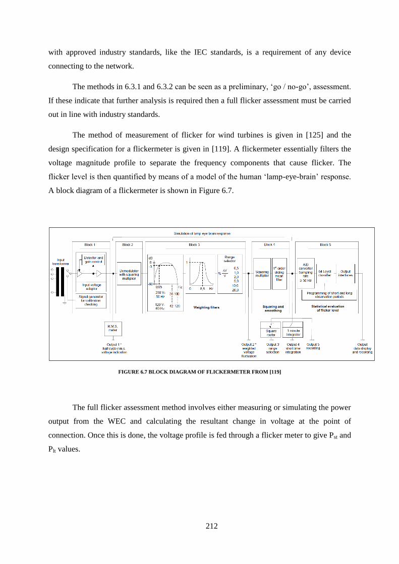
212
with approved industry standards, like the IEC standards, is a requirement of any device
connecting to the network.
The methods in 6.3.1 and 6.3.2 can be seen as a preliminary, ‘go / no-go’, assessment.
If these indicate that further analysis is required then a full flicker assessment must be carried
out in line with industry standards.
The method of measurement of flicker for wind turbines is given in [125] and the
design specification for a flickermeter is given in [119]. A flickermeter essentially filters the
voltage magnitude profile to separate the frequency components that cause flicker. The
flicker level is then quantified by means of a model of the human ‘lamp-eye-brain’ response.
A block diagram of a flickermeter is shown in Figure 6.7.
FIGURE 6.7 BLOCK DIAGRAM OF FLICKERMETER FROM [119]
The full flicker assessment method involves either measuring or simulating the power
output from the WEC and calculating the resultant change in voltage at the point of
connection. Once this is done, the voltage profile is fed through a flicker meter to give Pst and
Plt values.

213
6.4 Case Study: Wavebob
A case study is undertaken here to show the use of the flicker assessment tools
discussed in Section 6.3 and also to assess, for an actual grid connected wave energy
converter, the severity of the flicker for the entire scatter diagram. This illustrates the sea-
states that induce the largest flicker emission levels.
The case study considers the Wavebob WEC at the European Marine Energy Centre
(EMEC) test site. The characteristics for the case study are given in Table 6.4. These values
are derived from information provided by Wavebob and EMEC.
TABLE 6.4 PARAMETERS FOR CASE STUDY
Wavebob @ EMEC
ΔSn/Sk 0.00164 %
Pst and Plt limits in the jurisdiction 1.0
Grid X/R Ratio 1.87
WEC Power Factor (cosθ) 1
6.4.1 Basic Flicker Assessment
Using Equation 6.2, the potential voltage variation ΔU/U is calculated as 0.164%.
This is below the level of any issue with flicker, 0.85%. Therefore, this basic assessment
shows that the case study WEC does not present any issue with flicker. There are, however,
issues with this basic assessment method that make it unsuitable and the flicker assessment
charts should be used.
6.4.2 Flicker Assessment Charts
The relevant flicker assessment chart is given in Figure 6.3 where the Pst limit is 1.0
and is reproduced with the result in Figure 6.6 in Section 6.3.3. The ΔSn/Sk percentage in this
case is 0.00164% and the X/R ratio is 1.87. This means that the intersection point for these
values is below the line for ‘cosθ = 1’. Therefore, from the flicker assessment charts it is

214
apparent that the case study WEC does not present any issue with flicker. This is expected as
the ratio of Sn/Sk is very small in this case study. Normally, this would indicate that no further
assessment is required.
6.4.3 Full Flicker Assessment
No further assessment would normally be required for this case study due to the large
Sk/Sn ratio and hence no flicker issue.
Nevertheless, in order to investigate the flicker emissions from the WEC further, a
full assessment was carried out with the grid fault level/WEC rated power ratio (Sk/Sn) set to
1.0 and the X/R ratio set to 1.2 (ψk = 50°). This gives the ‘flicker coefficient’, c (Ψk), for all
the sea-states at the site. The X/R ratio chosen is one of several recommended X/R ratios
given in [125].
The ‘flicker coefficient’, c(Ψk) , is a non site specific (i.e. generic) value and can be
divided by the actual Sk/Sn ratio for any site to give the actual Pst values, at the same
impedance phase angle (Ψk), for that site.
The assessment was carried out using time domain simulations of the Wavebob WEC
(un-tuned) at the EMEC test site. The original scatter from [128] is adapted to use custom
intervals for Hs and Tp values, suitable for the Wavebob in-house simulations tools and is
shown in Figure 6.8. This shows that the highest occurring sea-states are at lower period (Tp :
5.5-8.5 seconds)
FIGURE 6.8 SCATTER DIAGRAM FROM EMEC ADAPTED FROM [128]
5.75 0.01 0.03 0.19 0.36 0.50 0.25 0.12 0.08
5.25 0.00 0.01 0.03 0.42 0.37 0.10 0.04 0.01 0.01
4.75 0.01 0.10 0.32 0.55 0.41 0.08 0.03 0.01 0.02
4.25 0.01 0.01 0.40 1.29 0.66 0.26 0.06 0.04 0.02 0.02
3.75 0.01 0.31 0.96 2.03 0.80 0.21 0.06 0.02 0.01 0.01
3.25 0.02 0.09 1.44 2.22 1.64 0.60 0.14 0.07 0.03 0.02 0.02
2.75 0.14 0.73 2.53 2.95 0.85 0.37 0.14 0.09 0.05 0.02 0.02
2.25 0.06 0.76 3.49 3.37 2.28 0.81 0.40 0.20 0.12 0.06 0.02 0.02
1.75 0.71 2.12 5.12 3.65 1.73 0.77 0.41 0.19 0.09 0.03 0.01 0.02
1.25 2.27 4.89 5.16 3.49 1.81 0.84 0.42 0.17 0.07 0.04 0.01 0.02
0.75 6.26 9.13 6.34 3.69 1.75 0.81 0.46 0.26 0.15 0.07 0.02 0.01
5.50 6.50 7.50 8.50 9.50 10.50 11.50 12.50 13.50 14.50 15.50 16.50
Annual Occurrence % (Total = 100%)
Tp [s]
Hs [m]

215
A 10 minute simulated power output time series from the device was evaluated and
the c(Ψk) calculated for each of the cells in the scatter diagram, i.e. each sea-state. The
voltage variation was calculated using the same formula from [123] presented Section 6.1.1.3
and the Pst value was calculated using a third party IEC flicker assessment software program
[129], [130]. This software program calculates the Pst value in line with the relevant IEC
standard.
The flicker coefficient for the scatter diagram is presented in Figure 6.9 with the
characteristics shown in Table 6.5.
TABLE 6.5 PARAMETERS FOR CF CALCULATION
Wavebob @ EMEC
ΔSn/Sk 100% (make ΔSn = Sk for c(Ψk) calculation)
Grid X/R Ratio 1.2 (ψk = 50°)
WEC Power Factor (cosθ) 0.98 lagging
FIGURE 6.9 C(ΨK) FOR WAVEBOB, (ΨK = 50°)
What is evident in Figure 6.9 is that the more severe flicker occurs at the lower period
(higher frequency) sea-states (<10 seconds). This is expected as the flicker limits are lower
5.75 31.86 29.78 23.4 19.31 14.85 13.02 8.58 7.17
5.25 33.34 30.56 25.03 21 16.46 12.78 9.84 8.49 6.72
4.75 30.98 26.17 20.88 18.79 15.08 10.46 8.96 7.25 5.93
4.25 29.96 27.07 22.45 21.23 15.62 11.69 8.54 7.21 5.32 4.17
3.75 26.63 24.41 18.72 15.29 13.11 8.82 8.8 5.89 4.83 3.42
3.25 28.19 23.27 19.13 15.55 13.25 8.87 6.89 5.4 4.01 2.96 2.6
2.75 20.82 18.48 16.48 10.71 8.74 7.35 5.14 3.94 3.31 2.65 1.74
2.25 14.55 15.79 15.1 11.28 9.17 5.04 4.58 3.72 2.63 2.26 1.83 1.48
1.75 10.7 12 8.29 6.58 4.87 3.43 2.95 2.12 1.77 1.29 0.92 0.87
1.25 6.28 6.66 5.44 3.96 2.6 2.17 1.7 1.06 1 0.65 0.64 0.45
0.75 2.73 2.22 2.03 1.43 1.06 0.97 0.48 0.4 0.34 0.26 0.25 0.23
5.50 6.50 7.50 8.50 9.50 10.50 11.50 12.50 13.50 14.50 15.50 16.50
Tp (s)
Hs (m)
Flicker Coefficient, c(ψk)

216
for higher frequencies in the area of interest shown in Figure 6.2. As the significant wave
height, Hs, becomes larger and therefore the sea-state contains more energy, the flicker
becomes more severe at higher period (low frequency) sea-states. However, this is only to a
point as the highest period (lowest frequency) sea states exhibit a drop off in flicker severity,
even for large Hs values.
In Figure 6.9 the highest flicker coefficient is 33.34 (Hs = 5.25, Tp = 8.5). For a Pst
limit of 1.0, what can be inferred is that the Wavebob device exceeds the flicker limits for
any Grid Fault Level/WEC Rated Power Ratio (Sk/Sn) of less than 33.34, given an X/R ratio
of 1.2 (ψk = 50°) and power factor of 0.98 lagging. Using this c(Ψk) value for the EMEC case
study shown in Table 6.4 it is clear that the maximum flicker emission, Pst , at EMEC for the
Wavebob device would be 0.0546 (c(Ψk) / (Sk/Sn) = 33.36/610), for Ψk of 50°, which is well
below the limit of 1.0. This verifies our initial assessments in 6.4.1 and 6.4.2
It should be noted that this simulation is a ‘un-tuned’ Wavebob WEC. The Wavebob
WEC can be tuned with the opening, partial opening and closing of its submerged tank.
When tuned, the response of the WEC could be reduced for higher energy sea-states meaning
a potential reduction in the maximum flicker coefficient witnessed.
For this worst case cell (Hs = 5.25, Tp = 8.5) other X/R ratios and power factors are
evaluated. As per [125] a range of typical X/R Ratios are evaluated, namely 0.57 (ψk = 30°),
1.2 (ψk = 50°), 2.7 (ψk = 70°), and 11.4 (ψk = 85°). Also a range of power factors are
evaluated between 0.95 lagging and 0.95 leading. The results are plotted in Figure 6.10.
Figure 6.10 shows that the flicker coefficient becomes smaller as the X/R ratio
becomes larger and also, that as the power factor changes from lagging to leading the flicker
coefficient becomes smaller. This coincides with the results shown in the flicker assessment
charts in Figure 6.3, Figure 6.4 and Figure 6.5.
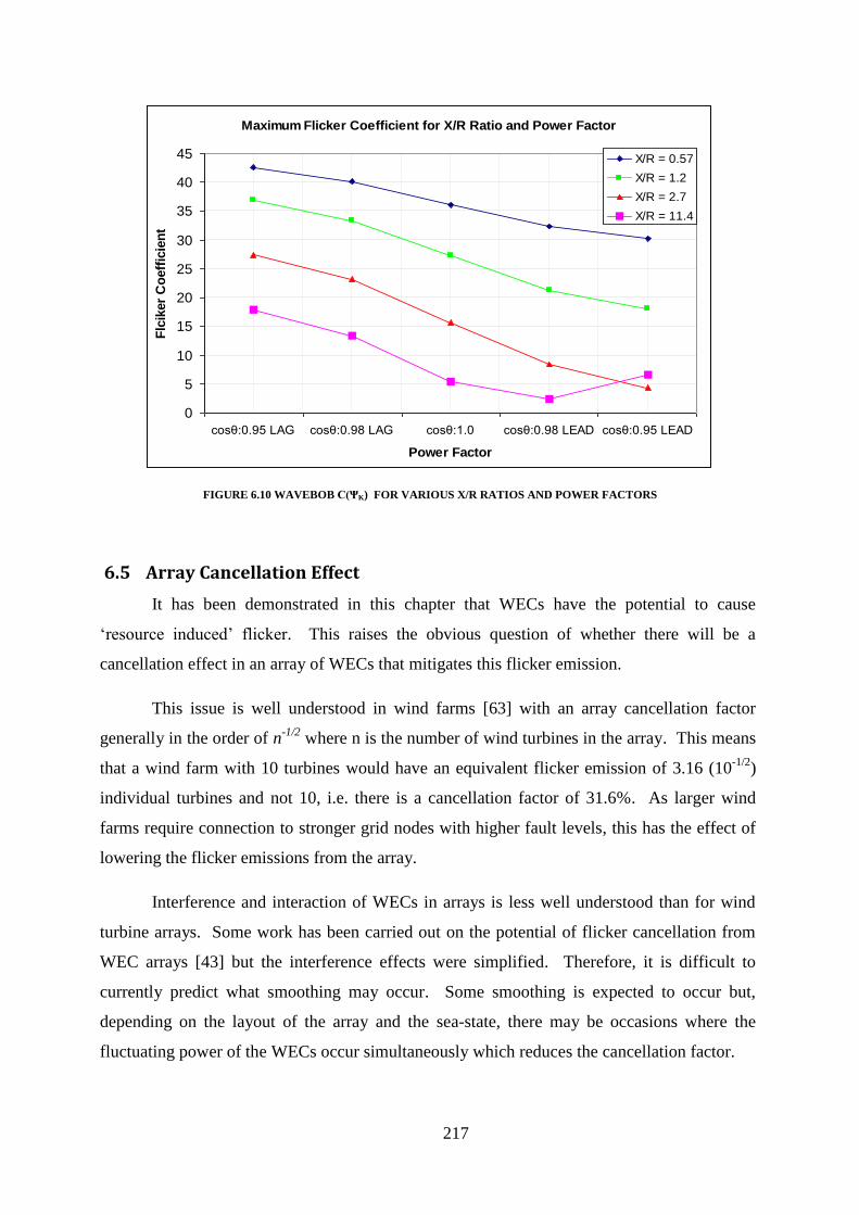
217
FIGURE 6.10 WAVEBOB C(ΨK) FOR VARIOUS X/R RATIOS AND POWER FACTORS
6.5 Array Cancellation Effect
It has been demonstrated in this chapter that WECs have the potential to cause
‘resource induced’ flicker. This raises the obvious question of whether there will be a
cancellation effect in an array of WECs that mitigates this flicker emission.
This issue is well understood in wind farms [63] with an array cancellation factor
generally in the order of n-1/2
where n is the number of wind turbines in the array. This means
that a wind farm with 10 turbines would have an equivalent flicker emission of 3.16 (10-1/2
)
individual turbines and not 10, i.e. there is a cancellation factor of 31.6%. As larger wind
farms require connection to stronger grid nodes with higher fault levels, this has the effect of
lowering the flicker emissions from the array.
Interference and interaction of WECs in arrays is less well understood than for wind
turbine arrays. Some work has been carried out on the potential of flicker cancellation from
WEC arrays [43] but the interference effects were simplified. Therefore, it is difficult to
currently predict what smoothing may occur. Some smoothing is expected to occur but,
depending on the layout of the array and the sea-state, there may be occasions where the
fluctuating power of the WECs occur simultaneously which reduces the cancellation factor.
Maximum Flicker Coefficient for X/R Ratio and Power Factor
0
5
10
15
20
25
30
35
40
45
cosθ:0.95 LAG cosθ:0.98 LAG cosθ:1.0 cosθ:0.98 LEAD cosθ:0.95 LEAD
Power Factor
Flc
iker
Co
eff
icie
nt
X/R = 0.57
X/R = 1.2
X/R = 2.7
X/R = 11.4

218
It is likely that the cancellation factor for WEC arrays is somewhere between n-1/2
and
1 (i.e. no smoothing), depending on numerous factors in the configuration of the array.
6.6 Flicker Mitigation
If the resource induced flicker from a WEC exceeds the local emission limits then
there are several possibilities for overcoming this. Some of these have been discussed
previously in [131].
6.6.1 Energy Storage/Smoothing:
An energy storage system could be installed either on the WEC device itself or at the
point of connection (POC) to smooth the power fluctuations and hence reduce flicker if
necessary. There are several options available for energy storage. Mechanical storage
solutions are available such as flywheels or hydraulic accumulators. Electrical and
electrochemical storage solutions are also possible such as capacitors or battery energy
storage. Each storage solution has characteristics which dictate its suitability, or
unsuitability, for overcoming flicker from a WEC. The suitability of a storage solution for
operation in the marine environment shall also be an important factor if the storage system is
to be installed within the WEC.
The storage system has to be fast acting and rated for the amplitude of the power
fluctuation. It is also subjected to multiple cycles during its lifetime. The addition of storage
inevitably means additional cost and an efficiency reduction in the overall system which
needs to be factored into any techno-economic analysis of the overall WEC system.
6.6.2 Spatial Configuration (Cancellation Effect)
As discussed in Section 6.5 when the cancellation effects in WEC arrays are better
understood, it may be possible to reduce flicker by an appropriate spatial design of the array.
219
6.6.3 Control Strategy
A control strategy could be implemented in certain situations that not only reduces
power fluctuation from individual devices [132] but also varies the characteristic responses of
devices in a WEC array to avoid a statistical summing of power fluctuations and maximise
the flicker cancellation factor.
In general, control systems may control a WEC for maximum energy absorption and
conversion or could control a WEC for continuous power output (i.e. minimise fluctuations).
A storage system, or inherent storage (e.g. hydraulic accumulators), may be required to allow
the control of the WEC for continuous power output. Controlling a WEC to minimise power
fluctuations at the output could reduce overall energy production for a WEC at a given site.
This should be factored into the overall techno-economic analysis of the WEC system.
6.6.4 Reactive Power Compensation
Another possibility to counter a power fluctuations problem is the addition of a
controlled reactive power device such as a STATCOM at the POC [133], [134]. This can
instantaneously control the import and export of reactive power (VARs) from/to the grid and
hence control the voltage level to be sufficiently smooth at the POC. So as the active power
from the WEC fluctuates the reactive power from the STATCOM also fluctuates
proportionally. The net result would be that even though the active power from the WEC
continues to fluctuate, the STATCOM negates the effect this has on voltage at the POC.
Like energy storage, this solution means additional costs and losses in the overall
system. This must be factored into the overall techno-economic analysis of the WEC system.
6.6.5 Increasing Short Circuit Power
By reconfiguring the network at the POC or by the reinforcing the network up to the
POC, the fault (short circuit) level can be increased meaning that the power fluctuations
would not affect the voltage as severely. This would typically mean the installation of
additional overhead lines and transformers to strengthen the connection to the WEC array.
Any costs for additional overhead lines, transformers or switchgear would typically be
passed onto the project developer. Therefore, this solution is likely to be the most costly of
those suggested in this section.

220
6.7 Conclusion
Flicker is a power quality issue that any renewable power generator needs to consider.
Flicker is of particular interest in wave energy due to the fact that ‘resource induced’ flicker
lies in the frequency range of the flicker curve.
As flicker assessment can be complicated and specialised a number of options for
assessing flicker are presented. These range from a preliminary calculation, the use of
bespoke flicker assessment charts, and a full flicker assessment. The simplicity of the flicker
assessment charts should allow for any party to evaluate the potential flicker from a wave
energy converter at a given site. This facilitates an understanding of flicker impacts at an
early stage in the design process.
A case study was undertaken to show the use of these methods. However, the case
study WEC was shown, with the flicker assessment graphs, to not have a flicker issue at the
specified site. This is due to the very large Sk/Sn ratio.
The flicker coefficient, c(Ψk), was evaluated for the case study WEC according to IEC
standards. The flicker coefficient can be used to evaluate flicker at different sites in the
future. This flicker coefficient showed that the ‘resource induced’ flicker is higher at lower
period waves and particularly at high energy (high Hs), low period (low Tp) waves.
There are several possibilities for mitigating these flicker issues and the cancellation
of flicker within an array is not yet fully understood. However, most mitigation strategies
would have a cost and efficiency penalty on the overall system.

221
7 The Domestic and Export Market for Irish Wave Energy
Chapter 7
The Domestic and Export Market for
Irish Wave Energy
7.1 Introduction
There is an abundant wave energy resource surrounding Ireland and, given mature
and cost effective technology, this could be accessed as renewable electrical energy. A
concentrated effort is underway in the wave energy industry to develop reliable and efficient
conversion technology and begin to develop early stage projects.
In Ireland, the renewable generation industry is dominated by onshore wind and this
industry looks set to continue to grow even to a saturation point in terms of energy demand,
and power system stability. The wind industry in Ireland is already looking to export markets
for future growth.
Assuming that the right technology is available in the future to exploit the abundant
wave energy resource in Ireland, this chapter examines where the market for this generated
energy may be, and what technical, and economic, barriers exist to accessing this market.
7.2 Wave Energy Resource and Location in Ireland
The energy density of a given sea-state is calculated as a function of the wave height
(in metres) and the wave period (in seconds). The annual average wave energy resource is
expressed as kilowatts per metre (kW/m) and the resource off the west coast of Ireland is one
of the highest energy resources in the world with a deep-water annual average resource of
70kW/m or higher off the west coast. This is shown in Figure 7.1.

222
FIGURE 7.1 GLOBAL ANNUAL WAVE ENERGY RESOURCE (KW/M) (SOURCE: OCEANENERGY.IE)
It is important to differentiate between the theoretical resource and the practical or
accessible resource. The theoretical resource is the energy that is available in the ocean
waves and assumed unlimited deployment of wave energy converters (WECs) absorbing all
available energy. The practical accessible resource is the energy that can be extracted and
converted to electrical energy and is a small fraction of the theoretical resource. The practical
resource is constrained by the WEC technology utilised and any local constraints such as
shipping lanes, fishing zones, or areas of conservation.
A comprehensive study of the wave energy potential in Ireland was undertaken by
ESB International [7] indicating that the theoretical annual wave energy resource in Ireland
was 525TWh. This is within an electrical energy market with an annual demand of 34.5TWh
in 2012 [135]. Thus, the available theoretical energy far exceeds the domestic Irish demand.
However, from ESB International’s report [7], the practical accessible resource is 21TWh.
This represents 4% of the theoretical resource but over 60% of the total electrical energy
demand of Ireland in 2012.
7.3 Hypothetical WEC Arrays for Analysis
The practical accessible resource of 21TWh corresponds to an annual average power
output of around 2.4GW. Assuming a potential capacity factor of 40% for WEC arrays off
the Irish west coast, this corresponds to a total practical installed capacity of 6GW. This

223
represents the full exploitation of the practical resource in Ireland. It should be noted that the
definition of practical resource may change based on market conditions, i.e. deeper water
sites may become commercially viable or technology performance improves.
For the purposes of analysis this total capacity of 6GW is split into three candidate
WEC arrays off the Irish west coast, each with a peak capacity of 2GW which, as explained
in Section 7.6.1 is a viable transmission rating for HVDC transmission. The three areas for
the WEC arrays were chosen to be roughly at the location of the Marine Institute data buoys
M4 (NW Array), M1 (W Array) and M3 (SW Array). See Figure 7.2 for the location of these
data buoys.
The Marine Institute data buoys are located in deeper water than would be expected
for WEC arrays. The chosen locations of the three candidate WEC arrays can be seen in
Figure 7.3 and are located around the 100m depth contour.
Although the candidate arrays are 2GW per array, it is expected that a 2GW array
would not be installed as a first project in a single location. The scenario here is a
hypothetical maximum utilisation of the practical accessible resource.
FIGURE 7.2 LOCATIONS OF MARINE INSTITUTE DATA BUOYS (WWW.MARINE.IE)

224
FIGURE 7.3 LOCATIONS OF THREE 2GW CANDIDATE WEC ARRAYS
7.4 2020 Targets and Wind Development in Ireland
In 2010, the gross final energy use from renewable sources in Ireland was 5.5% with
the percentage of electrical generation capacity from renewables at 15% [136]. The 2020
target for gross final energy use under the EU Renewable Energy Directive 2009/28/EC is
16% for Ireland. In order to achieve this, 40% of electrical generation capacity must be from
renewable sources by 2020. Based on the median demand forecast it is expected that 3.5-
4GW of renewable energy will be required to meet this level of electrical generation from
renewables.
In 2014, the EU began the process of defining the approach to emission reductions
and renewable energy for 2030 [137]. The targets within the framework are not as clearly
defined as the 2020 targets but call for an EU reduction in greenhouse gas emissions of 40%
(over 1990 levels) by 2030, an increase in renewable energy to 27% of total energy usage,
and an increase in energy efficiency by 30%. It remains to be seen how these EU wide
targets will be translated into policy and renewable energy targets at a national level.
Ireland is on course to meet our 2020 target from onshore wind alone, and this has
certainly been the focus of domestic energy policy. There is over 2GW of wind energy
currently installed within the single electricity market (SEM). There is close to an additional

225
4GW planned within the group processing approach known as Gate 3 (3.2GW of onshore
wind and 0.8GW of offshore wind) [138].
Beyond Gate 3 there is a further 12GW of planned onshore wind in the ‘queue’,
sometimes referred to informally as Gate 4. Gate 4 projects will not be processed until Gate
3 has been completed.
On top of the projects in Gate 3 and Gate 4, there are additional projects planned that
involve onshore wind in Ireland with direct export to the UK. Projects such as Greenwire
[139], Energy Bridge [140], Marex [141] and Natural Hydro Energy [142] plan to offer wind
energy to the UK market at a more competitive price than the UK would have to pay for
offshore wind in its own territory. These projects have potential of up to 10GW beyond what
is in Gate 3 and Gate 4. However, these projects are yet to receive clear approval from the
Irish or UK government as of 2014.
It is clear then that Ireland has enough wind in planning to meet and far exceed its
2020 targets and not only provide enough renewable energy for the domestic market but
potentially exploit this renewable energy for export. It is expected, however, that some of the
proposed wind generation capacity in Gate 3, Gate 4 and the export projects will not be
developed. The development of these projects depends on the market conditions, success in
planning permission, and grid access among many other factors.
In order to facilitate the proposed volume of wind energy on the Irish electricity
system, some important changes are currently taking place. Firstly, the transmission system
needs to be upgraded to accommodate large volumes of wind in locations remote from
demand centres. Secondly, the system needs to be designed to operate securely with large
proportions of non-synchronous generation.
Eirgrid's Grid25 strategy [143] provides for the reinforcement of the transmission
system in Ireland to assist in the exploitation of wind energy. Much of this reinforcement
work is presently taking place to facilitate Gate 3 connections.
Another issue with high levels of wind on the system is the power system stability
from high penetration of non-synchronous generation. High penetration of non-synchronous
generation means a low system inertia that can cause system frequency stability issues during
loss of generation or faults.

226
At present there is an imposed limit for non-synchronous generation. This requires
that system non-synchronous penetration (SNSP) must not exceed 50% of the instantaneous
system demand. This means that if non-synchronous generation capacity, predominantly
wind, is more than 50% of instantaneous system demand, the instantaneous wind generation
must be curtailed thus losing potential generation and revenue for wind farm owners. In
2012, 2.1% of all potential renewable energy generation in the SEM was curtailed [144].
Eirgrid [145] outlines a plan to enable this limit to be increased to 75%. However,
even with this strategy some curtailment is still likely, and, as the capacity of wind generation
grows, curtailment may increase and the revenue of wind plant would thus be reduced,
perhaps to the point where investment in new renewable generation will suffer.
7.5 Wave Energy Opportunities in the Irish Market
In Section 7.4, the current market for wind in Ireland was outlined. There is currently
around 16% wind energy as a proportion of total generation in Ireland and there are plans to
increase this to 40%. At present, some curtailment of wind energy, due to system stability
issues, is already in place and this may increase with further wind capacity. Wind farm
developers are now looking to export markets for opportunities as the Irish market may
provide limited opportunities beyond what is planned.
It is not certain, therefore, where wave energy fits into this market. Certainly it is
expected that large scale WEC arrays are not be possible until after 2020 as WEC technology
is still developing. The Irish domestic renewables market may be heavily saturated with
wind energy when the time comes to begin large scale WEC arrays.
From this information it seems that the domestic market for wave energy may be
limited, certainly over the next two decades. There may, however, be some opportunity for
wave energy in the domestic Irish market as outlined in the scenarios below.
7.5.1 Non-Concurrence and Diversity
Waves are, like wind, an intermittent renewable source. Nevertheless, the physics of
wave generation are different than wind energy and the intermittency may be non-concurrent
with wind energy. So high and low outputs of WEC arrays may not occur with highs and
lows of wind farms. This can be exploited in a number of ways:

227
Firstly, the addition of diversity into the renewable energy mix is likely to reduce
overall intermittency and the need for thermal backup [104], [146]. It should be noted
that diversity of renewables, will not allow a higher SNSP, if all renewables remain
non-synchronous.
Secondly, expensive transmission infrastructure, for bringing remote output from
wind farms to demand centres, can be shared with wave installations thus increasing
the utilisation of the infrastructure [104].
There is likely to be several system wide benefits by adding wave energy to the
domestic renewable energy mix. In the long term this could allow a more secure and cost
effective electrical system.
7.5.2 Additional Interconnection and Storage in the System
Albeit, mostly focussed on market integration, the addition of more interconnection
into the Irish system from neighbouring markets (UK and France) will certainly reduce the
requirements for curtailment and allow greater penetration of renewables in the Irish
domestic market [147]. HVDC interconnectors may also have the ability to provide
‘synthetic’ inertia, to increase the limits for non synchronous generation still further.
Large scale energy storage, such as pumped storage facilities, may allow the
conversion of non-synchronous intermittent generation into dispatchable synchronous
generation within the Irish market. Power-to-gas type schemes may also permit inter-
seasonal storage. Large scale energy storage has the potential to dramatically change the
market for renewables in Ireland and Europe, but the economic case to support this is not
currently viable.
There are a number of ways a fully integrated system could develop with
interconnection, storage and large penetration of renewables; however this is not the topic of
this chapter.
7.5.3 Re-use of redundant infrastructure.
Some transmission infrastructure may become redundant as thermal plants on the
west coast of Ireland are decommissioned. An example of this is the Moneypoint power

228
station which was commissioned in the mid 1980s and has recently undergone a retrofit and
installation of flue gas abatement systems. It is possible that the existing Moneypoint plant
will be decommissioned in the mid-2020s, as it will be 40 years old by this point, and there
are two dedicated 400kV lines from the plant (located on the west coast) to Dublin (the main
load centre in Ireland) as shown in Figure 7.4.
The decommissioning of a station like Moneypoint may provide a ready asset for
transmission; however the market and system issues will still apply.
FIGURE 7.4 LOCATION OF MONEYPOINT AND ROUTE OF 400KV LINES TOWARDS DUBLIN
7.5.4 Synchronous Wave Energy Converters
Wind turbines use non-synchronous generators and WECs are also expected to be
non-synchronous generators based on current designs of prototypes. If WECs can be
designed with synchronous generators then they would assist in system frequency support
and may not be limited by curtailment. This may be possible for some hydraulic PTO type
WECs as described in Section 3.2.1.3.

229
7.5.5 Irish Domestic Market for Ocean Energy Summary
As outlined in the above sections there is likely to be only a limited domestic market
for wave energy in Ireland given the current market outlook. The addition of wave energy to
the renewables mix may reduce intermittency, and could increase utilisation of exiting
transmission infrastructure. If there is a limited domestic market for wave energy then an
export market must be explored.
7.6 Export Market Opportunities
If the abundant wave energy resource off the west coast of Ireland cannot be exploited
domestically, due to market and system issues, then an export solution must be explored. The
UK is the geographically closest market to Ireland with France being the next closest.
2020 targets for gross energy from renewable sources are 15% in the UK and 23% in
France. In the UK, this dictates a target of 30% of electricity generation from renewable
sources by 2020. In France, this target is 27%. As of 2010, the UK reached 6.7% (towards a
target of 30%) and France reached 14.5% (towards a target of 27%) of electrical generation
from renewables [148].
These 2020 targets may present a challenge for both the UK and France, and imports
of renewable electricity generation from Ireland could help them meet their 2020 targets and
beyond. This is an opportunity for export of renewable energy from Ireland that is already
being considered by the wind export projects presented in Section 7.4. It is important to note
however that the cost of importing these renewables to the importing nation will be a critical
factor to the potential of an export market for Irish renewables.
If wave energy cannot access the domestic market in Ireland, for the reasons outlined
in previous sections, then it may require access to these export markets.
7.6.1 HVDC Technology and Costs
There are two ways in which wave energy off the west coast of Ireland can access
export markets. Firstly, through an integrated export network through the Irish system which
would require multiple interconnections between the Irish and export markets. This is a
likely scenario to develop over the longer term.

230
Secondly, through dedicated transmission infrastructure from the WEC array to the
export market. As explained previously, a fully integrated system may evolve in a number of
ways and is not the topic of this chapter. Dedicated transmission for WEC array export
systems however will be evaluated further here.
Due to the large submarine distances and large power capacities required for the
candidate WEC arrays, High Voltage Direct Current (HVDC) transmission would be the only
potential transmission solution for connecting Irish WEC arrays directly to the UK and
France. HVDC transmission systems allow the long distance overland or submarine transfer
of bulk electrical power. Over long distances they are more efficient and cost effective than
High Voltage Alternating Current (HVAC) systems. HVDC transmission involves
converting electrical power from AC to DC for transmission, then back to AC for connection
to the grid at the other end. Figure 7.5 shows a representative HVDC transmission system,
FIGURE 7.5 TYPICAL HVDC TRANSMISSION SYSTEM (COURTESY WIKIPEDIA)
HVDC cabled transmission systems are possible up to around 2.5GW per system
[149], which is at the upper limit of the converter and cable technology. This was part of the
rationale for splitting the 6GW of potential wave energy capacity into three 2GW WEC
arrays for analysis.
The cost elements of HVDC systems to transmit power from WEC array projects with
export to the UK would fall into the following categories:
HVDC Converter Stations

231
Offshore Platform – At WEC array end only
Offshore cables
Onshore cables
From [149], [150], [151], [152] & [153] reference costs were established for these
components and are presented in Table 7.1. All reference costs are for 2GW systems only.
Note that component costs are for reference only and there can be large variations across
projects depending on market conditions, route characteristics, vessel requirements among
many other aspects. Note also that a cost of €20m is estimated for an offshore platform for
HVDC converter, i.e. the platform structure only.
TABLE 7.1 COST REFERENCES FOR HVDC TRANSMISSION
Component Reference
Cost
Unit
HVDC Converter
Stations
0.15 m€/MW
Offshore Platform 20 m€/platform
Offshore HVDC Cables 2.0 m€/km
Onshore HVDC Cables 2.2 m€/km
There would also be a large cost for the WEC array electrical network that would
involve the connection of the WECs in circuits to a central offshore substation and
connection from that substation to the HVDC export transmission system. The cost of this
array’s electrical system is not considered here as this would also be required for a typical
WEC array connected to the local grid and therefore is not an additional cost.
7.7 Case Study: Wave Array Export Transmission to UK and France
The previous sections demonstrated that a limited domestic market in Ireland may
lead to exploring export markets and HVDC transmission would be an enabling technology

232
for this. This section outlines the projected costs of such transmission systems for accessing
export markets.
In Figure 7.6 the three proposed 2GW WEC arrays are shown (‘NW’, ‘W’ and ‘SW’
WEC Arrays from Figure 7.3) and five export access zones are shown (Z1-5). These access
zones are chosen as the closest location to the WEC arrays that have access to Extra High
Voltage (EHV – 380kV or higher) grids. As illustrated in Figure 7.6 seven routes were
evaluated between the WEC arrays and the various zones.
FIGURE 7.6 LOCATIONS OF CANDIDATE WEC ARRAYS AND POTENTIAL CONNECTIONS TO EXPORT MARKETS
The distance between the WEC Arrays and the relevant access zones was calculated
using an online mapping tool. Straight line distances were calculated but these are increased
by 20% to allow for expected route length increase over point to point distances. Within each
zone there may be several connection nodes to the EHV grid and the range of costs given are
for the closest node and the furthest node within the zone.
Table 7.2 shows the calculated capital costs for the seven export routes depicted in
Figure 7.6. This presents the total cost of the offshore platform (€20m) at the WEC array, the
offshore HVDC converter, the total cable route length (including onshore and offshore), and
NW
W
SW
Z1
Z2
Z3
Z4
Z5

233
the onshore HVDC converter at the access zones. The costs presented in Table 7.1 are used
to establish these capital costs.
TABLE 7.2 CAPITAL COSTS FOR HVDC TRANSMISSION SYSTEM FOR WEC ARRAY EXPORT
From WEC
Array
To Zone Capital Cost
Total
Capital Cost per MW
(2GW system)
NW Z1 €1.3 – 1.47bn €0.65 – 0.74m
NW Z2 €1.22bn €0.61m
NW Z3 €1.55 – 1.58bn €0.77 – 0.79m
W Z3 €1.55bn €0.77m
SW Z3 €1.68bn €0.84m
SW Z4 €1.55 – 1.91bn €0.78 – 0.96m
SW Z5 €2.19bn €1.1m
Note that the per-MW figures are based on a 2GW system. It is expected that these
costs do not scale linearly so would not be valid for a 500MW system, for example. This
shows that for an export market to be exploited large scale WEC arrays are necessary to
dilute the additional cost of the export system
7.8 Conclusion
It is well documented that Ireland has an abundant wave energy resource and with
suitable and cost effective WEC technology this can be exploited for renewable electrical
power generation.
Ireland has other abundant renewable resources, notably wind power. It is likely that
onshore wind can meet Irish domestic demand for renewable electrical generation up to 2020.
Domestic demand for renewables will be dictated by the growth in electrical demand and also

234
by how much non-synchronous generation can be tolerated before power system stability
becomes an issue.
The domestic market for wave energy may be limited in Ireland through saturation
with onshore wind, system stability issues, or other causes. There is opportunity to export to
neighbouring markets, namely the UK and France, to assist these countries increasing their
penetration of renewable energy resources. Viable HVDC technology can connect the long
distances and large power capacities to these neighbouring markets. However, there is an
additional cost, for transmission systems, associated with accessing these export markets.
The cost of such systems could range from €1.2 – 2bn depending on the distance
between the WEC array and the export market. This adds €0.6 – 1.1m / MW onto the capital
cost of a WEC array project, which may be an unacceptable increase. This is based on a
2GW capacity and this scale of transmission is required to minimise the costs per MW which
would increase for smaller capacities.
In order for wave energy from Ireland to be an attractive proposition for export
markets, it is expected that it must be as commercially attractive as other forms of renewable
energy. In this regard, offshore wind is a good benchmark. Current capital costs of offshore
wind are approximately €4m / MW [151]. Therefore, in order to be commercially attractive
for export, wave energy projects, including the cost of export transmission, must compete
with these costs. The export system alone could comprise 25% or higher of the overall
capital costs of potential projects. Thus, the challenge for cost effective WEC arrays may
become more difficult given the additional ‘export premium’ cost.
Ireland has an enviable wave energy resource and there are many challenges in
exploiting this, including developing cost effective WEC technology. A major challenge is in
understanding where the long-term market lies for wave energy from Ireland. This chapter
concludes that for large scale wave energy, the long-term market is an export one. This
brings additional cost to any proposed large scale WEC array.
235
8 Conclusions and Future Work
Chapter 8
Conclusions and Future Work
8.1 Discussion, Conclusion, and Contribution of Thesis
In this thesis, a comprehensive analysis has been undertaken of some key grid
integration issues for WEC arrays. This thesis enhances the knowledge base in the subject
area of WEC array electrical networks, WEC voltage flicker emission assessment, and the
domestic and export market for wave energy in Ireland.
The objectives of this thesis are set out in Chapter 1 and in this Chapter it is assessed how
these objectives have been met. The objectives are reproduced below.:
Develop technically and economically acceptable electrical network designs for
WEC arrays considering;
o Economic constraints
o Array technical requirements
o Array functional requirements
o Experience to date from both the offshore wind industry and the wave energy
industry
o Potential strategies for improving economics for WEC electrical networks
Evaluate voltage flicker issues for WEC arrays and develop design tools to analyse
same.
Evaluate the market scale for wave energy in Ireland, considering electrical
integration issues in both the domestic and export markets.

236
8.1.1 Techno-Economic Optimisation
Objective:
Develop technically and economically acceptable electrical network designs for
WEC arrays considering;
o Economic constraints
o Array technical requirements
o Array functional requirements
o Experience to date from both the offshore wind industry and the wave energy
industry
o Potential strategies for improving economics for WEC electrical networks
This objective has been achieved by firstly developing a comprehensive
understanding of a wide range of considerations to be made when designing an optimum
electrical network for WEC arrays. These are introduced in Chapter 3 and Chapter 4.
In Chapter 3, the state-of-the-art in WEC on-board systems and components, WEC
array components, and WEC test sites and prototype electrical networks has been introduced
and analysed. The state-of-the-art in offshore wind farm electrical networks has also been
introduced and analysed. Although there are divergent concepts in the area of WEC
electrical networks, there is much more convergence in electrical network design in the
offshore wind industry and there is certainly cross-over possible, particularly the rationale
behind design convergence, and with installation vessels and processes. The key differences
between offshore wind farm and WEC array electrical networks have been shown to occur at
‘key interfaces’ which are critical in the techno-economic optimisation outlined in Chapter 4.
A techno-economic analysis of WEC array electrical network concepts has been
detailed in Chapter 4. At the beginning of Chapter 4, the technical and economic
considerations for the design and optimisation of WEC array electrical networks have been
outlined. By introducing and analysing potential options for both the key interfaces and the
WEC array electrical network configurations, a techno-economic optimisation has been
carried out.

237
It has been concluded that radial network configurations are the optimum
configuration for WEC arrays. However, some deficiencies with this configuration must be
addressed, notably the lack of redundancy. Strategies for addressing these deficiencies have
been introduced. Optimised key interfaces for a radial network have been presented that
allow a WEC array electrical network to be realised within target costs while maintaining
critical functionality.
The annual average network efficiency has been calculated for a number of candidate
WEC arrays (10MW, 40MW and 150MW). This has demonstrated that network efficiency
of up to 99% can be expected for the optimised WEC array electrical network. It has been
noted that an understanding of the generation characteristic of the WECs within the array is
critical to calculate network efficiency. Array spacing and operating voltage have negligible
impact on efficiency, but affect the economics of the array.
The expected costs for the optimised array electrical network have been calculated
and are shown to be on target for commercial WEC arrays, i.e. €1m/MW.
The economic challenges for WEC array electrical networks are introduced and some
strategies to improve the economics analysed has been shown in Chapter 5. Design criteria
such as WEC device rating, WEC capacity factor, array spacing, and site conditions have
been shown to influence the economics of the WEC array electrical network. These design
criteria can increase or decrease WEC array electrical network cost. Therefore, WEC and
WEC array designers must balance the impact any design decisions have on the WEC array
electrical network economics against any potential benefits.
Also in Chapter 5, some strategies for improving the economics of WEC array
electrical networks have been introduced and evaluated. By understanding the characteristics
of the WEC array, the electrical network can be under-rated to allow lower cost with minimal
curtailment. Also, by applying dynamic ratings on the electrical network or using more
sophisticated real time thermal rating systems, the electrical network can be utilised fully
without risk of exceeding safe operating conditions. This may result in the reduction of
electrical network ratings and hence a reduction in cost.
The objective to Develop technically and economically acceptable electrical network
designs for has been achieved within Chapters 3-5 of this thesis.

238
8.1.2 Voltage Flicker Evaluation
Objective:
Evaluate voltage flicker issues for WEC arrays and develop design tools to analyse
same.
The issue of voltage flicker is prevalent for any renewable generator with a variable
input resource. It has been demonstrated in Chapter 6 that for wave energy, there is a
potential coupling of input resource, ocean waves, to output power. As the input resource lies
within the frequency of interest for voltage flicker, it has been shown that it is highly likely
that WEC devices will create flicker emissions.
The assessment and quantification of flicker emissions is a requirement for any
renewable generator but the process is complicated. In order to allow early assessment of
flicker emissions at design stage, a flicker assessment tool has been developed and its use is
also outlined in Chapter 6. This tool is not a substitute for international standards but is a
design tool.
A full flicker evaluation case study has also been undertaken in Chapter 6 to further
understand the relationship between the resource and potential flicker emissions. It has been
demonstrated that flicker emissions are higher at lower period (high frequency) input
resource. In particular low period, high energy (i.e. high Hs) resource causes the highest
levels of flicker emission. There are potential mitigation strategies for flicker but it has been
shown that these may incur a cost or efficiency penalty.
The objective to Evaluate voltage flicker issues for WEC arrays and develop design
tools to analyse same has been achieved within Chapter 6 of this thesis.
239
8.1.3 Irish Market Evaluation
Objective:
Evaluate the market scale for wave energy in Ireland, considering electrical
integration issues in both the domestic and export markets.
In Chapter 7, the potential domestic and export market for wave energy in Ireland has
been assessed. In this chapter, the renewables market in Ireland is presented and it has been
shown that onshore wind may saturate and limit the market for renewables in Ireland over the
coming decades. Neighbouring markets such as the UK and France present an export
opportunity for wave energy from Ireland.
Due to the distances to these export markets, HVDC transmission technology has
been shown to be an enabling technology. This would enable access to export markets, but at
a cost. It is concluded that these transmission systems would costs €0.6-1.1m/MW depending
on transmission distance. Large WEC arrays would be required to dilute the cost of this
transmission infrastructure.
The objective to Evaluate the market scale for wave energy in Ireland, considering
electrical integration issues in both the domestic and export markets has been achieved
within Chapter 7 of this thesis.
8.1.4 Summary and Key Conclusions
The major important conclusions of this thesis are presented in Table 8.1. This
summarises the most important outcomes of the research in this thesis.

240
TABLE 8.1KEY CONCLUSIONS FROM THIS RESEARCH
Key Conclusions
Radial networks are the optimal network configuration for offshore WEC array electrical
networks
Electrical networks for WEC arrays can be achieved with high efficiency and at a cost to
allow a competitive wave energy industry
This competitiveness can be improved further by applying strategies to reduce the WEC array
electrical network capex.
Voltage flicker is demonstrated to be inherent and potentially severe for WEC output
Practical tools for assessing voltage flicker emissions from WECs have been presented
Voltage flicker is shown to be particularly severe for lower period sea states with large
significant wave height
While Ireland has an enviable wave resource, integrating this into the Irish electricity system
is challenging
Export markets are technically accessible but the cost of transmission is a barrier to
competitiveness
All of the above conclusions can be considered novel academic contributions and
provide solutions to important questions being asked by the wave energy industry. This
thesis provides guidance to WEC designers and WEC array designers and developers. This
achieves the objectives set out in Chapter 1 of this thesis and assures that this work adds
significantly to the knowledge base of the industry.
The thesis concludes that there are great challenges for wave energy in the area of
grid integration. Through careful design, optimisation and analysis, it is evident that cost
effective and technically suitable WEC arrays can be achieved.

241
8.2 Future Work
This thesis is practically focussed and therefore needs practical demonstration of the
research conclusions. This is not possible to do within the confines of this thesis as the costs
of demonstrating the suggested solutions would be excessive. As the wave energy industry
moves from the current prototyping focus towards commercial array deployment, there will
be an opportunity to review the findings of this research against practical applications. At
that time, a clearer understanding of some of the issues in this work will be possible.
It is apparent that the targeted sites for WEC array installation of the western seaboard
of Europe are exposed to extreme wave conditions. While this means that there is a large
wave energy resource to be exploited, it also presents challenges to the installation of
submarine electrical networks. A suggested follow-on research topic would be to analyse the
wave energy at a proposed site in order to understand the weather risk to cable installation.
This would involve exploring the requirements of cable installation vessels and undertaking a
persistence analysis on the site wave resource. Weather risk is likely to be a large challenge
and contractual issue for commercial arrays and a deeper understanding of this would be
valuable to the industry.
Another major challenge for large scale WEC arrays will be the realisation and cost of
offshore substations in deep water locations, which has been briefly assessed in this thesis. It
is suggested that the technical solutions and economics of offshore substations for WEC
arrays in 100m water depth should be explored as a detailed research topic. This is critical to
understand the competitiveness of wave energy in the longer term.
Radial networks are proposed in this work as the optimal solution for WEC array
electrical network configurations. There are deficiencies of radial networks in the areas of
redundancy and requirements for multiple connections to devices. Some strategies to
overcoming these deficiencies are presented in this research. A suggested follow on piece of
research would be to undertake a techno-economic evaluation of these, and other potential,
strategies to further understand the impact of this on the WEC array electrical system
economics and performance. Some practical demonstration of these solutions should form
part of this research.
It is clear from this work that the design of cost effective electrical networks will be
challenging. The sharing of this expensive offshore electrical infrastructure with either
offshore wind, solar, or tidal energy may ultimately improve the economics for wave energy.

242
A suggested follow-on piece of research would be to analyse the wind, wave, tidal and solar
energy potential at a number of sites to assess the viability of a ‘shared’ electrical network
approach.
From this research, it is also clear that Ireland’s renewable energy mix is heavily
dependant on onshore wind energy and this has begun to influence system stability. The
introduction of wave energy to the Irish renewables mix may assist in reducing intermittency
within the power system and help with system stability. It has also been documented that
wave energy is a more predictable renewable resource. A suggested follow-on piece of
research would be to assess the value of adding a range or proportions of wave energy to the
Irish renewable energy mix.

243

244
Bibliography
[1] International Energy Agency - Ocean Energy Systems, “Ocean Energy Systems
Annual Report 2012,” IEA-OES, 2012.
[2] R. Green and N. Vasilakos, “The Economics of Offshore Wind,” Energy Policy,
vol. 39, pp. 496-502, 2010.
[3] RenewableUK, “Channelling the Energy - A Way Forward for the UK Wave &
Tidal Industry Towards 2020,” 2010.
[4] W. Dick, “Wave Energy Converter”. U.S.A. Patent 6857266, 2005.
[5] A. Clement and et al, “Wave energy in Europe: current status and perspectives,”
Renewable and Sustainable Energy Reviews, vol. 6, no. 5, pp. 405-431, 2002.
[6] The Crown Estate, “Wave and Tidal Energy in the Pentland Firth and Orkney
Waters: How the Projects Could be Built,” The Crown Estate, 2011.
[7] ESBI, “Accessible Wave Energy Resource Atlas: Ireland: 2005,” 2005.
[8] Carbon Trust, “UK Wave Energy Resource,” 2012.
[9] V. deLaleu, Électricité de France, 2009. [Online]. Available: http://www.inter-
mines.org/docs/0904140804PR_090319_DeLaleu.pdf. [Accessed November
2013].
[10] Elfosk, “Wave Power - Surveilance Study of the Development,” 2011.
[11] RenewableUK, “Wind Energy in the UK. State of the Industry Report,” 2012.
[12] RenewableUK, “Offshore Wind Forecasts of future costs and benefits,” 2011.
[13] T. W. Thorpe, “An Overview of Wave Energy Technologies: Status, Performance
and Costs,” in IMECHE Seminar - Wave Power - Moving Towards Commercial
Viability, 1999.
[14] National Oceanic and Atmospheric Administration, “Ocean Service Education,”

245
[Online]. Available:
http://oceanservice.noaa.gov/education/kits/currents/media/supp_cur03a.html.
[Accessed July 2014].
[15] European Commission, “Wave Energy Brochure,” [Online]. Available:
http://ec.europa.eu/energy/res/sectors/doc/ocean/wave_energy_brochure.pdf.
[Accessed July 2014].
[16] J. Falnes, Ocean Waves and Oscillating Systems, Cambridge University Press,
2002.
[17] R. Alcorn and D. O Sullivan, Electrical Design for Ocean Wave and Tidal Energy
Systems, Institute of Engineering and Technology, 2013.
[18] R. Speirs, D. Wilson and H. Whittingtom, “Electrical Generation Systems Suitable
for Use in Wave Power Schemes,” in Edinburgh Wave Power Project, 1977.
[19] D. O'Sullivan and G. Dalton, “Challenges in the Grid Connection of Wave Energy
Devices,” in 8th European Wave and Tidal Energy Conference (EWTEC), 2009.
[20] D. O'Sullivan and A. Lewis, “Generator Selection for Offshore Oscillating Water
Column Wave Energy Converter,” in 13th Power and Motion Control Conference,
2008.
[21] D. O'Sullivan and A. Lewis, “Electrical Machine Options in Offshore Floating
Wave Energy Converter Turbo Generators,” in World Renewable Energy
Congress, 2008.
[22] M. Mueller, H. Polinder and N. Baker, “Current and Novel Electrical Generator
Technology for Wave Energy Converters,” in IEEE International Electric
Machines & Drives Conference, 2007.
[23] M. A. Mueller, “Electrical Generator for Direct Drive Wave Energy Converters,”
Generation, Transmission and Distribution, vol. 109, no. 4, pp. 446-456, 2002.
[24] J. Shek, D. Macpherson, M. Mueller and J. Xiang, “Reaction force control of a
linear electrical generator for direct drive wave energy conversion,” IET
Rewewable Power Generation, vol. 1, no. 1, pp. 17-24, 2007.

246
[25] J. Fletcher, T. Judendorfer, M. Mueller, N. Hassanain and M. Muhr, “Electrical
issues associated with sea-water immersed windings in electrical generators for
wave and tidal current-driven power generation,” IET Renewable Power
Generation, vol. 3, no. 2, pp. 254-264, 2009.
[26] M. Leijon, O. Danielsson, M. Eriksson, K. Thorburn, H. Bernhoff, J. Isberg, J.
Sundberg, I. Ivanova, E. Sjostedt, O. Agren, K. Karlsson and A. Wolfbrandt, “An
electrical approach to wave energy conversion,” Renewable Energy, vol. 31, no. 9,
pp. 1309-1319, 2006.
[27] M. Leijon, C. Bostrom, O. Danielsson, S. Gustafsson, K. Haikonen, O.
Langhammer, E. Stromstedt, M. Stalberg, J. Sundberg, O. Svensson and R. W. S.
Tyrberg, “Wave Energy from the North Sea: Experiences from the Lysekil
Research Site,” Surveys in Geophysics, vol. 29, no. 3, pp. 221-240, 2008.
[28] O. Danielsson, M. Leijon and E. Sjostedt, “Detailed study of the magnetic circuit
in a longitudinal flux permanent-magnet synchronous linear generator,” IEEE
Transactions on Magnetics, vol. 41, no. 9, pp. 2940-2495, 2005.
[29] C. Bostrom, B. Ekergard, R. Waters, M. Eriksson and M. Leijon, “Linear
Generator Connected to a Resonance-Rectifier Circuit,” IEEE Journal of Oceanic
Engineering, vol. 38, no. 2, pp. 255-262, 2013.
[30] O. Danielsson, “Wave Energy Conversion - Linear Synchronous Permanent
Magnet Generator - PhD Thesis,” Uppsala University, Stockholm, 2006.
[31] M. Eriksson, “Modelling and Experimental Verification of Direct Drive Wave
Energy Conversion - Buoy-Generator Dynamics - PhD Thesis,” Uppsala
University, Stockholm, Sweden, 2007.
[32] R. Waters, “Energy from the Ocean Waves - Full Scale Experimental Verification
of a Wave Energy Converter - PhD Thesis,” Uppsala University, Stockholm,
Sweden, 2008.
[33] M. Santos, D. B. Haim, F. Salcedo, J. Villate and Y. Torre-Enciso, “Grid
Integration of Wave Energy Farms: Basque Country Study,” in 3rd International
Conference on Ocean Energy, Bilbao, Spain, 2010.

247
[34] T. Boehme, G. Harrison and A. Wallace, “Assessment of distribution network
limits for non-firm cconnection of renewable generation,” IET Renewable Power
Generation, vol. 4, no. 1, pp. 64-74, 2010.
[35] J. Khan, D. Leon, A. Moshref, S. Arabi and G. Bhuyan, “Electricity System
Scenario Analysis to Determine Level of Wave Power that Can be Integrated: a
Case Study,” in 3rd International Conference on Ocean Energy, Bilbao, Spain,
2010.
[36] T. Ahmed, K. Nishida and M. Nakaoka, “The Potential for Grid Power Integration
of Offshore Ocean Wave Energy in the UK,” in International Power Electronics
Conference, 2010.
[37] A. Blavette, D. O'Sullivan, M. Egan and A. Lewis, “Grid Compliance of Ocean
Energy Converters: Control Strategies and Reccomendations,” in European Wave
and Tidal Energy Conference, 2011.
[38] A. Blavette, D. O'Sullivan, M. Egan, A. Lewis and R. Alcorn, “Wave Energy Grid
Integration in Ireland – A Case Study,” in 3rd International Conference on Ocean
Energy (ICOE), Bilbao, Spain, 2010.
[39] A. Nambiar, A. Kiprakis, D. Forehand and A. Wallace, “Effects of Array
Configuration, Network Impacts and Mitigation of Arrays of Wave Energy
Converters Connected to Weak, Rural Electricity Networks,” in 3rd International
Conference on Ocean Energy (ICOE), Bilbao, Spain, 2010.
[40] A.Kiprakis, A. Nambiar, D. Forehand and A. Wallace, “Modelling Arrays of Wave
Energy Convertes Connected to Weak Rural Electrical Networks,” in International
Conference on Sustainable Power Generation and Supply, 2009.
[41] A. Nambiar, A. Kiprakis and A. Wallace, “Voltage quality control of a 1MW wave
farm connected to weak, rural electricity networks,” in 45th International
Universities Power Engineering Conference (UPEC), 2010.
[42] A. Nambiar, A. Kaprakis and A. Wallace, “Quantification of voltage fluctuations
caused by a wave farm connected to weak, rural electrical networks,” in 14th
International Conference on Harmonics and Power Quality, 2010.

248
[43] A. Blavette, D. O'Sullivan, A. Lewis and M. Egan, “Impact of a Wave Farm on its
Local Grid: Voltage Limits, Flicker Level and Power Fluctuations,” in IEEE/MTS
OCEANS Conference, Yeosu, South Korea, 2012.
[44] A. Blavette, D. O'Sullivan, A. Lewis and M. Egan, “Grid Integration of Wave and
Tidal Energy,” in ASME 30th International Conference on Ocean, Offshore and
Arctic Engineering, Rotterdam, The Netherlands, 2011.
[45] D. Murray, M. Egan, J. Hayes and D. O'Sullivan, “Applications of Supercapacitor
Energy Storage for a Wave Energy Converter System,” in 8th European Wave and
Tidal Energy Conference, Uppsala, Sweden, 2009.
[46] S. Muthukumar, S. Kakumanu, S. Sriram and V. Jayashankar, “Energy Storage
Considerations for a Standalone Wave Energy Plant,” in IEEE International
Conference on Electric Machines and Drives, San Antonio, Texas, 2005.
[47] S. Muthukumar, S. Kakumanu, S. Sririam, R. Desai, A. Babar and V. Jayashankar,
“On Minimizing the Fluctuations in the Power Generated from a Wave Energy
Plant,” in IEEE International Conference on Electric Machines and Drives, San
Antonio, TX, 2005.
[48] A. Blavette, D. O'Sullivan, A. Lewis and M. Egan, “Dimensioning the Equipment
of a Wave Farm: Energy Storage and Cables,” in 8th International Conference and
Exhibition on Ecological Vehicles and Renewable Energies (EVER), 2013.
[49] University of Edinburgh, “Wave Energy Report on the Electrical Aspects of the
Edinburgh University Wave Energy Device,” Edinburgh Wave Power Project,
1979.
[50] A. Wallace, “Design Considerations of Submarine Power Links,” Edinburgh Wave
Power Project, 1976.
[51] J. Lopez, P. Ricci, J. Villate, A. Bahaj, L. Myers, C. Retzler and J. Dhedin,
“Preliminary economic assessment and analysis of grid connection schemes for
ocean energy arrays,” in 3rd International Conference on Ocean Energy (ICOE),
Bilbao, Spain, 2010.
[52] L. Myers, A. Bahaj, C. Retzler, P. Ricci and J. Dhedin, “Inter-device spacing

249
issues within wave and tidal energy converter arrays,” in 3rd International
Conference on Ocean Energy (ICOE), Bilbao, Spain, 2010.
[53] P. Ricci, B. Counago, A. Rico, J. Villante and Y. Torre-Enciso, “Alternatives for
the Design of Grid Connection Infrastructures for Wave Energy,” in 3rd
International Conference on Ocean Energy (ICOE), Bilbao, Spain, 2010.
[54] L. Martinelli, A. Lamberti, P. Ruol, P. Ricci, P. Kirrane, C. Fenton and L.
Johanning, “Power Umbilical for Ocean Renewable Energy Systems - Feasibility
and Dynamic Response Analysis,” in 3rd International Conference on Ocean
Energy (ICOE), Bilbao, Spain, 2010.
[55] I. Lopez, J. Andreu, S. Ceballos, I. M. d. Alegria and I. Kortabarria, “Review of
wave energy technologies and the necessary power-equipment,” Renewable and
Sustainable Energy Reviews, vol. 27, pp. 413-434, 2013.
[56] P. Igic, Z. Zhou, W. Knapp, J. MacEnri, H. Sorensen and E. Friis-Madsen, “Multi-
megawatt offshore wave energy converters - electrical system configuration and
generator control strategy,” IET Renewable Power Generation, vol. 5, no. 1, pp.
10-17, 2011.
[57] M. Kenny, “Electrical Connection Issues for Wave Energy Arrays - Masters
Thesis,” University College Cork, 2010.
[58] K. Thorburn, H. Bernhoff and M. Leijon, “Wave energy transmission system
concepts for linear generator arrays,” Ocean Engineering, vol. 31, pp. 1339-1349,
2004.
[59] M. Rahm, C. Bostrom, O. Svensson, M. Grabbe, F. Bulow and M. Leijon,
“Offshore underwater substation for wave energy converter arrays,” IET
Renewable Power Generation, vol. 4, no. 6, pp. 602-612, 2009.
[60] C. Bostrom, E. Lejerskog, M. Stalberg, K. Thorburn and M. Leijon, “Experimental
results of rectification and filtration from an offshore wave energy system,”
Renewable Energy, vol. 34, pp. 1381-1387, 2008.
[61] Equimar, “Deliverable 5.1 - Guidance protocols on choosing of electrical
connection configurations,” 2009.

250
[62] Wavenet, “Deliverable F3 - Power transmission from Wave Power Plants,” 2003.
[63] T. Ackermann, Wind Power in Power Systems, John Wiley and Sons, 2005.
[64] J. Twidell and G. G, Offshore Wind Power, Multi-Science Publishing, 2007.
[65] B. Franken, H. Breder, M. Dahlgren and E. Nielsen, “Collection Grid Topologies
for Offshore Windparks,” in 18th International Conference on Electricity
Distribution, 2005.
[66] I. M. d. Alegria, J. Martin, I. Kortabarria, J. Andreu and P. I. Ereno, “Transmission
Alternatives for Offshore Electrical Power,” Renewable and Sustainable Energy
Reviews, vol. 13, no. 5, pp. 1027-1038, 2009.
[67] J. Green, A. Bowen, L. Fingersh and Y. Wan, “Electrical Collection and
Transmission Systems for Offshore Wind Power,” in Offshore Technology
Conference, 2007.
[68] J. Yang, J. O'Reilly and J. Fletcher, “Redundancy Analysis of Offshore Wind Farm
Collection and Transmission Systems,” in International Conference on
Sustainable Power Generation and Supply, 2009.
[69] O. Holmestrom and N. Negra, “Survey of Reliability of Large Offshore Wind
Farms,” in European Wind Energy Conference, Milan, Italy, 2007.
[70] N. Negra, J. Todorovic and T. Ackermann, “Loss Evaluation of HVAC and HVDC
Transmission Solutions for Large Offshore Wind Farms,” Electric Power Systems
Research, vol. 76, no. 11, pp. 916-927, 2006.
[71] N. Boccard, “Capacity Factor of Wind Power Realized Values versus Estimates,”
Energy Policy, vol. 37, pp. 2679-2688, 1009.
[72] C. Fitzgerald and G. Thomas, “A Preliminary Study on the Optimal Performance
of an Array of Wave Power Devices,” in 7th European Wave and Tidal Energy
Conference (EWTEC), Porto, Portugal, 2007.
[73] J. Fitzgerald, “Position Mooring of Wave Energy Converters - PhD Thesis,”
Chalmers University, 2009.
[74] J. Fitzgerald and L. Bergdahl, “Considering Mooring Cables for Offshore Wave

251
Energy Converters,” in 7th European Wave and Tidal Energy Conference
(EWTEC), Porto, Portugal, 2007.
[75] B. Child and V. Venugopal, “Optimal Configuration of Wave Energy Device
Arrays,” Journal of Ocean Engineering, vol. 37, no. 16, pp. 1402-1417, 2010.
[76] P. Ricci, J. Saulnier and A. Falcao, “Point Absorber Arrays: A Configuration
Study off the Portugese West Coast,” in 7th European Wave and Tidal Energy
Conference, Porto, Portugal, 2007.
[77] J. Cruz, R. Sykes, P. Siddorn and R. Taylor, “Estimating the loads and Energy
Yields of Arrays of Wave Energy Converters under Realistic Seas,” IET
Renewable Power Generation, vol. 4, no. 6, pp. 488-497, 2010.
[78] J. Westphalen, G. Bacelli, P. Balitsky and J. Ringwood, “Control Strategies for
Arrays of Wave Energy Converters,” in European Wave and Tidal Energy
Conference, 2011.
[79] T. Seppa, “Increasing Transmission Capacity by Real Time Monitoring,” in IEEE
Power Enegineering Society Winter Meeting, 2002.
[80] S. Walldorf, A. Ernst and S. Pancholi, “A Cost Effective Solution for Increasing
Ratings on Underground Transmission Cables - A Case Study,” in IEEE
Transmission and Distribution Conference, 1999.
[81] B. Grotenhuis, J. Jaspers, A. Kerstens, A. v. d. Wey and F. Wild, “Increasing the
Capacity of Cable Systems Using Cable Asset Management Based on Thermal and
Mechanical Properties,” in IEEE International Conference on Electrical
Distribution, 2001.
[82] J. Downes and H. Leung, “Distributed Temperature Sensing Worldwide Power
Circuit Monitoring Applications,” in International Conference on Power Systems
Technology, 2004.
[83] “Artemis Intellegent Power,” [Online]. Available: http://www.artemisip.com/.
[Accessed August 2013].
[84] Nexans, “Submarine Power Cables Specifications,” 2008.

252
[85] L. Stenberg, “Wave Power Cable Connection - Masters Thesis,” Royal Institute of
Technology, Sweden, 2009.
[86] RenewableUK, “Offshore Wind and Marine Energy Health and Safety
Guidelines,” 2013.
[87] “Guidelines for Grid Connection of Marine Energy Conversion Systems,”
European Marine Energy Centre, 2009.
[88] C. Bartzsch, H. Huang, T. Westerweller and M. Davies, “HVDC Plus and SVC
Plus; Reliable and Cost-Effective Power Transmission Solutions with Modular
Multilevel Converters,” in Cigre Study Committee B4 - HVDC and Power
Electronics Colloquium 2011, 2011.
[89] “Beatrice Offshore Wind Demonstrator,” [Online]. Available:
www.beatricewind.co.uk. [Accessed August 2013].
[90] S. Breto and G. Moe, “Status, Plans and Technologies for Offshore Wind Turbines
in Europe and North America,” Renewable Energy, vol. 34, pp. 646-654, 2009.
[91] H. Landsverk, O. Granhuag, P. Skrten and S. Ranfoss, “36kV Vacuum Circuit
Breaker Panel - The Perfect Switchgear for Wind,” in 20th International
Conference on Electricity Distribution, Prague, Czech Republic, 2009.
[92] Z. Li, M. Zhao and Z. Chen, “Efficiency Evaluation for Offshore Wind Farms,” in
International Conference on Power System Technology, 2006.
[93] H. Brakelmann, “Efficiency of HVAC Power Transmission from Offshore
Windmills to the Grid,” in IEEE Power Tech Conference, Bologna, Italy, 2003.
[94] D. Mollison, “Ireland's Wave Power Resource - A report to the National Board for
Science and Technology and Electricity Supply Board,” NBST, 1982.
[95] J. Keller and B. Kroposki, “Understanding Fault Characteristics of Inverter-Based
Distributed Energy Resources,” National Renewable Energy Laboratory (NREL),
2010.
[96] G. J. Anders, Rating of Electric Power Cables - Ampacity Computations for
Transmission, Distribution and Industrial Applications, McGraw Hill, 1997.

253
[97] C. Moore, BICC Electrical Cables Handbook - 3rd Edition, Blackwell, 1997.
[98] International Electrotechnical Commission, “IEC 60287. Electrical Cables –
Calculation of the Current Rating”.
[99] ABB, “XLPE Submarine Cable Systems - Attachement to XLPE Land Cable
Systems - User's Guide,” 2010.
[100] S. Lundberg, “Performance Comparison of Wind Park Configurations - PhD
Thesis,” Chalmers University, 2003.
[101] The Centre for Sustainable Electricity and Distributed Generation, “Cost Benefit
Methodology for Optimal Design of Offshore Transmission Systems,” 2008.
[102] Department of Trade and industry (UK), “Study of the Costs of Offshore Wind
Generation,” 2007.
[103] M. Banzo and A. Ramos, “Stochiastic Optimisation Model for Electric Power
System Planning for Offshore Wind Farms,” IEEE Transactions on Power
Systems, vol. 26, no. 3, pp. 1338-1348, 2010.
[104] E. Stoutenburg and M. Jacobson, “Optimizing Offshore Transmission Links for
Marine Renewable Energy Farms,” in OCEANS, 2010.
[105] ESB International, “Atlantic Marine Energy Centre Cable Options Report,” 2009.
[106] “Pelamis Installation System,” [Online]. Available:
http://www.pelamiswave.com/our-technology/installation. [Accessed August
2013].
[107] “Siemens Subsea Power Grid,” [Online]. Available:
http://www.energy.siemens.com/hq/en/industries-utilities/oil-
gas/applications/subsea-power-grid.htm. [Accessed August 2013].
[108] “ABB – Controlled Subsea Electric Power Distribution with SEPSIS,” [Online].
Available:
http://www05.abb.com/global/scot/scot271.nsf/veritydisplay/84915130ebc8aa87c1
256ef50045878f/$File/36-42%20-%20M147.pdf. [Accessed August 2013].
[109] “GE Vetco Gray - Subsea Power Systems,” [Online]. Available: http://www.ge-

254
energy.com/products_and_services/products/subsea_power_and_processing_syste
ms/index.jsp. [Accessed August 2013].
[110] “MacArtney Medium Voltage Hub,” [Online]. Available:
http://www.macartney.com/systems/infrastructure/terminations/medium-voltage-
hub. [Accessed August 2013].
[111] “Ocean Power Technologies - Underwater Subsation Pod,” [Online]. Available:
http://www.oceanpowertechnologies.com/pod.html. [Accessed August 2013].
[112] ABB, “Cables for Offshore Wind Brochure”.
[113] J. Beale, “Transmission Cable Protection and Stabilisation for the Wave and Tidal
Energy Industries,” in 10th European Wave and Tidal Energy Conference
(EWTEC), Southampton, UK, 2011.
[114] National Grid (UK), “Round 3 Offshore Wind Farm Connection Study,” 2010.
[115] J. Candido and J. Justino, “Frequency, stochastic and time domain models for an
articulated wave power device,” in ASME 27th International Conference on
Offshore Mechanics and Arctic Engineering (OMAE), 2008.
[116] International Electrotechnical Commission, “IEC 60853. Calculation of the Cyclic
and Emergency Current Ratings of Cables”.
[117] M. Luton, G. Anders, J. Braun, N. Fujimoto, S. Rizzetto and J. Downes, “Real
Time Monitoring of Power Cables by Fibre Optic Technologies. Tests,
Applications and Outlook,” in International Conference on Insulated Power
Cables, 2003.
[118] A. Baggini, Handbook of Power Quality, John Wiley & Sons, 2008.
[119] International Electrotechnical Commission, “IEC 41000-4-15. Electromagnetic
compatibility (EMC) - Part 4: Testing and Measurement Techniques - Section 15:
Flickermeter: Functional Design and Specification”.
[120] ESB Networks, “Distribution Code - Version 2.0,” 2007.
[121] The Electricity Council, “Engineering Recommendation P28 - Planning Limits for
Voltage Fluctuations Caused by Industrial, Commercial and Domestic Equipment

255
in the United Kingdom,” 1982.
[122] International Electrotechnical Commission, “IEC 61000-3-7. Electromagnetic
compatibility (EMC) - Part 3-7: Limits - Assessment of emission limits for the
connection of fluctuating installation to MV, HV and EHV power systems,” 2008.
[123] A. Larsson, “The Power Quality of Wind Turbines - PhD Thesis,” Chalmers
University, Gothenberg, Sweden, 2000.
[124] International Electrotechnical Commission, “PT 62600-30. Project Team for
Marine energy - Wave, tidal and other water current converters - Part 30: Electrical
power quality requirements for wave, tidal and other water current energy
converters,” Ongoing.
[125] International Electrotechnical Commission, “IEC 61400-21. Wind turbines - Part
21: Measurement and assessment of power quality characteristics of grid
connected wind turbines,” 2008.
[126] European Copper Institute, Power Quality Application Guide - Voltage
Disturbance - Flicker Measurement, 2005.
[127] British Standards Institution, “BS-EN 50160. Voltage Characteristics of Electricity
Supplied by Public Electricity Networks,” 2010.
[128] Equimar, “Deliverable D4.3 - Test Site Catalogue,” 2011.
[129] P. H. Ashmole, “Flicker Simulator Using UK Filter - Version 5.2,” 2000.
[130] P. Ashmole, “Quality of Supply - Voltage Fluctuations,” Power Engineering
Journal, vol. 14, no. 3, pp. 113-119, 2000.
[131] M. Lafoz, M. Blanco and D. Ramirez, “Grid Connection for Wave Power Farms,”
in 2011, Birmingham, UK, 14th European Conference on Power Electronics and
Applications.
[132] M. Santos, E. Tedeschi, P. Ricci, M. Molinas and J. Martin, “Grid Connection
Improvement by Control Strategy Selection for Wave Energy Converters,”
Renewable Energy and Power Quality, vol. 9, pp. 1-6, 2011.
[133] M. Barnes, R. El-Feres, S. Kromlides and A. Arulampalam, “Power Quality

256
Improvement for Wave Energy Converters using a D-STATCOM with Real
Energy Storage,” 1st European Conference on Power Electronic Systems and
Applications, 2004.
[134] A. Wallace and A. Kiprakis, “Reduction of voltage violations from embedded
generators connected to the distribution network by intelligent reactive power
control,” in 5th International Conference on Power System Management and
Control, London, 2002.
[135] Eirgrid plc, “Annual Report,” 2012.
[136] Department of Communications, Energy and Natural Resources, “Strategy for
Renewable Energy: 2012-2020”.
[137] European Commission, “2030 Framework for Climate and Energy Policies,” 2014.
[Online]. Available: http://ec.europa.eu/clima/policies/2030/index_en.htm.
[Accessed October 2014].
[138] Eirgrid plc, “Gate 3 ITC Programme Final Results Scheduled Firm Access
Quantities”.
[139] “Greenwire Project Website,” [Online]. Available: www.greenwire.ie. [Accessed
Auguse 2013].
[140] “Energy Bridge project website,” [Online]. Available: www.energybridge.ie.
[Accessed August 2013].
[141] “Marex project website,” [Online]. Available: www.organicpower.ie. [Accessed
August 2013].
[142] “Natural Hydro Energy project website,” [Online]. Available:
www.naturalhydroenergy.com. [Accessed August 2013].
[143] Eirgrid plc, “Grid25 - A Strategy for the Development of Ireland's Electricity Grid
for a Sustainable and Competitive Future”.
[144] Eirgrid plc, “2012 Curtailment Report,” 2013.
[145] Eirgrid plc, “All Island TSO Facilitation of Renewables Study”.

257
[146] F. Fusco, G. Nolan and J. Ringwood, “Variability reduction through optimal
combination of wind/wave resources - an Irish case study,” Energy, vol. 35, pp.
314-325, 2010.
[147] Eirgrid plc, “Interconnection Economic Feasibility Report,” 2009.
[148] “European Renewable Energy Statistics,” [Online]. Available:
http://epp.eurostat.ec.europa.eu/statistics_explained/index.php/Renewable_energy
_statistics . [Accessed August 2013].
[149] CIGRE, “Technical Brochure 492: Voltage Source Converter (VSC) HVDC for
Power Transmission - Economic Aspects and Comparison with other AC and DC
Technologies,” 2012.
[150] Irish-Scottish Links on Energy Study (ISLES), “Route Development and Cost
Estimation Report”.
[151] The Crown Estate, “Guide to an Offshore Wind Farm,” 2011.
[152] Institute of Engineering and Technology (IET), “Electricity Transmission Costing
Study,” 2012.
[153] National Grid UK, “Offshore Development Information Statement”.

258
Appendices

259

260
Appendix A – List of Publications
Below is a list of publications by the thesis author which relate to the research within this
thesis. Links to an online copy of each publication is provided for reference.
Journal Papers:
1. F. Sharkey, J. MacEnri, E. Bannon, M. Conlon and K. Gaughan, “Resource-induced
voltage flicker for wave energy converters – assessment tools,” IET Renewable Power
Generation,” vol. 7, no. 6, pp 623-630, 2013
http://arrow.dit.ie/engscheleart2/74/
2. F. Sharkey, E. Bannon, M. Conlon and K. Gaughan, “Maximising value of electrical
networks for wave energy converter arrays,” International Journal of Marine Energy,
vol. 1, no. 1, pp 55-69, 2013
http://arrow.dit.ie/engscheleart2/73/
Book Chapters:
1. F. Sharkey, “Electrical Design of Ocean Wave and Tidal Energy Systems – Chapter
10.1,” The Institute of Engineering and Technology, 2013
http://arrow.dit.ie/engschelebk/13/
Conference Papers:
1. F. Sharkey, M. Conlon and K. Gaughan, “Investigation of Wavefarm Electrical Network
Configurations,” in World Renewable Energy Congress, Linkoping, Sweden, 2011
http://arrow.dit.ie/engscheleart/161/
2. F. Sharkey, E. Bannon, M. Conlon and K. Gaughan, “Dynamic Electrical Ratings and the
Economics of Capacity Factor for Wave Energy Converter Arrays,” in 9th
European
Wave and Tidal Energy Conference, Southampton, UK, 2011

261
http://arrow.dit.ie/engscheleart/167/
3. F. Sharkey, M. Conlon and K. Gaughan, “Practical Analysis of Key Electrical Interfaces
for Wave Energy Converter Arrays,” in 4th
International Conference on Ocean Energy,
Dublin, Ireland, 2012
http://arrow.dit.ie/engscheleart/189/
4. F. Sharkey, J. MacEnri, E. Bannon, M. Conlon and K. Gaughan, “Voltage Flicker
Evaluation for Wave Energy Converters – Assessment Guidelines,” in 4th
International
Conference on Ocean Energy, Dublin, Ireland, 2012
http://arrow.dit.ie/engscheleart/188/
5. F. Sharkey, M. Conlon and K. Gaughan, “Impacts on the Electrical System Economics
from Critical Design Factors of Wave Energy Converters and Arrays,” in 10th
European
Wave and Tidal Energy Conference, Aalborg, Denmark, 2013
http://arrow.dit.ie/engscheleart/206/
6. F. Sharkey, K. Honer, M. Conlon, K. Gaughan and E. Robinson, “The Domestic and
Export Market of Large Scale Wave Energy in Ireland and the Economics of Export
Transmission,” in 48th
Universities’ Power Engineering Conference, Dublin, Ireland,
2013
http://arrow.dit.ie/engscheleart/207/

262

263