A Laboratory Evaluation of Unidata's Starflow Doppler Flowmeter and MGD Technologies Acoustic Doppler FlowMeter (ADFM)

By

Tracy B. Vermeyen, P .E. Water Resources Research Laboratory

Acknowledgments

This evaluation was funded by Reclamation's Water Measurement Research Program (project WR99.24). The Starflow equipment was loaned to Reclamation by Mr. Geoff Carrigg from Unidata America. Mr. Carrigg was very helpful in assisting with this evaluation and his agreement to loan Reclamation a Starflow system was greatly appreciated.. This evaluation was conducted because messrs. Brian Sauer (SRA-6414) and Mark Niblack (YA0-6020) were' interested in both acoustic flowmeters and wanted an independent test of the two systems. Mr. Cliff Pugh, Technical Specialist, peer reviewed this report.

Disclaimer: The information contained in this report regarding commercial products or companies may not be used for advertising or promotional purposes and is not to be construed as endorsement of any product or company by the U.S. Bureau of Reclamation.

Introduction

The Starflow ultrasonic Doppler instrument and the ADFM are unique devices which measure water velocity. depth, and temperature and they are integrated with data loggers. They are the first of a new generation of ultrasonic flow measurement systems.

Both systems use digital signal processing techniques, and they are able to perform in a wide range of environments. They can be used to record flows in pipes, channels and small streams and operates in a wide range of water qualities from fresh water to sewage channels.

These instruments represent two distinct types of Doppler instruments available to measure water velocity, they are:

WATER RESOURCES RESEARCH LABORATORY

OFFICIAL FILE COPY

STARFLOW

WATER SURFACE ,• ... · .. ,,•

. WATERVELOCITY .. : ;~,. ,--; .:: .'

..... · .... ,. ... ··~.:~~~ ·.; .~···: ., ...

. ' ... !" : ~

PARTICLE A

Figure I. Schematic of Starllow·s incoherent Doppler velocity measurement technique.

Figure 2. Photograph of the ADFM and Starllow transducers.

• Incoherent (or continuous) Dopplers. like the Startlow system, send out a continuous signal with one transmitter and measures signals n.:turning from scattercrs anywhere and everywhere along the beam \Vith a receiver, sec figures I and 2. The mcasun:d velocities of the particles are resolved to a mean velocity that can be related to a channel velocity at suitable sites. The Startlow system costs ahout S I. 700.

• Coherent (or profiling) Dopplers. like the 1\DFM. transmit encoded pulses with the carrier frequency along four beams and arc ahle to target specific locations (depth cells), and only measure these reflected signals. sec ligures 2 and 3. This allows the velocity in a stream to be profiled. These instruments are generally more complex and expensive when compared to incoherent Doppler systems. The ADFM system costs about $17,000.

Doppler-based Velocity Measurement Technique - During a measuring cycle, a ultrasonic pulse is transmitted at a fixed frequency. called the carrier frequency. A receiver listens for frequency shifts in reflected signals from any targets moving with the water. A measuring circuit detects the frequency changes. A processing system accumulates and analyses these frequency changes and calculates a representative Doppler shi it from the range received. Each Doppler shift is directly related to the water velocity componcnt along the beam. This is a physical relationship and ifyou know the speed of sound in \Vater )OU can calculate the velocity ofthe rellcctor (and thereby the velocity of the surrounding water). In general. the Starflow and ADFM instruments do not need calibration for velocity measurement.

More complete descriptions of both these instruments arc availahle in the appendices of this report.

2

Velocity Profile #1

Depth cells

l'igure 3. Cross section view of typical ADFM application. This figure shows the spatial relationship of the depth cells and the profiles relative to the transducer housing.

Discharge Computation Technique - Water depth (or stage) is measured and is used with a stage-area relationship to determine the cross sectional area of the flow measurement section. This stage-area relationship or cross section shape (e.g. circular or trapezoidal) are programmed into the flowmeter as part of the site information. Of course, the accuracy of this relationship is critical in the accuracy of the discharge computation. Each flowmeter system attempts to measure the average channel velocity using Doppler-based velocity measurement techniques. The cross sectional area and the average velocity measured by the instrument are multiplied to obtain a discharge.

Laboratory Evaluation

The Facilities- A side-by-side evaluation of the Starflow and ADFM was conducted in a flume in Reclamation's Water Resources Research Laboratory in Denver, Colorado. The rectangular flume dimensions are 8.5 ft wide and 4 ft deep and 60 ft long. The acoustic transducers were placed in the center of the channel about 20 ft downstream from the inlet transition. The pumped flow capacity to the flume is about 30 ft3/sec. The depth in the flume are controlled by tailboards used to change the open area of the channel at the end of the flume. The tailboards were located 40 ft downstream from the measurement section.

A second test was conducted in the WRRL's canal automation model. The rectangular canal cross section is 12-in wide and 18-in deep. The flow was set using a variable speed pump and a

3

calibrated propeller flowmeter. The propeller flowmeter was calibrated using a strap-on acoustic flowmeter and has an uncertainty of ±2 percent of the true discharge.

Testing Procedure- The first series of four tests were run over a range of flows and depths in a 8.5 ft wide flume. During each test, a Sontck ADV (acoustic Doppler Velocimeter) was used to measure an independent vertical velocity profile at the same location as the Starflow and ADFM. This ADV -measured profile was collected to determine the average velocity along the flume centerline to compare with the average velocity measured by the two instruments. Likewise, a staff gage was used to determine an independent measure of the depth at the measurement section. The average channel velocity was determined for each test by dividing the discharge by the cross sectional area. The average channel velocity is what the two flow meters need to accurately measure in order to calculate an accurate uncalibrated discharge.

An independent measure of the flowrate was made using the laboratory venturi measurement system which is accurate to ± 0.5%. This model also had flow delivered using auxiliary pumps and piping for tests 2 through 4. The flow through the auxiliary system was measured using a strap-on acoustic flowmeter which has an uncertainty of about ± 1- 2%. The com~ined discharge uncertainty for tests 2 through 4 was estimated to be± 1.4% (based on a 2% uncertainty for the strap-on acoustic flowmeter).

The second test was done in the WRRL's canal automation model with the discharge and depth held constant for 5 hours and 30 minutes. The Starflow was programmed collected data as fast a possible (5 second scan rate). This test was run to see how stable the Starflow's depth, velocity and discharge readings were with time.

Tests- Five tests were conducted in this evaluation. Both flowmeters were programmed to store data every 1 minute. The ADFM collected 160 profiles which were averaged prior to logging the data. The Starflow was set with a scan rate of 15 seconds, with about 500 velocity measurements per scan. The average depth and velocity for the four scans per minute were stored in the Starflow's data logger.

A fifth test was done to examine the long-term performance ofthe Starflow in the WRRL's canal automation model. The model is 12-in wide and 18-in deep. The flow was set at 1.0 ftl/sec and the water level was set at about 0.975 ft deep. Starflow data were logged at 5-second intervals and the scan rate was set to 5 seconds. This test represents the noisiest condition with respect to velocity measurement because it has the shortest sampling period allowable.

Test Results- Table 1 and figure 4 contain a summary of the data collected during the first four tests including percent error in the Starflow and ADFM measurements relative to the laboratory measured values. Table 2 and figure 5 contain a summary of the data collected during the fifth test including percent error in the Starflow measurements relative to the laboratory measured values.

4

Test Duration- For the first series of tests the duration of data collection varied. This is an important factor because acoustic velocity measurements depend on many individual samples to compute an accurate average velocity. In other words, a single Doppler velocity measurement is a degree of uncertainty, but the average of hundreds or thousands of measurements results in an accurate measure of the average velocity for the measurement period. Consequently, the results for these tests depend on the duration of the test and this showed up in the results. The duration of data collection for tests I through 4 were 60, 39, 20, and 50 minutes, respectively. This sampling length explains the difference in the ADFM's discharge uncertainty as presented in table I. The ADFM's discharge uncertainty was within ±3 percent of the laboratory discharge for the long duration tests and significantly greater than ±8 percent for shorter duration tests, namely tests 2 and 3. The average ADFM uncertainty over all four tests was+ 1.33 percent.

The discharge uncertainty for the Starflow meter appears to be inversely proportional to the test duration, which is a very peculiar characteristic. The Starflow's discharge uncertainty was greater than + 18 percent for all four tests. The average uncertainty in Starflow discharges over all four tests was + 26.2 percent.

The Starflow instrument systematically over predicted the depth and velocity for all tests. The ADFM systematically under predicted the depth, but the error in average velocity varied widely from test to test. Figure 6 shows a bar graph of the comparison of discharge, depth and velocity for the four flume tests.

In the fifth test, the Starflow instrument systematically over predicted the velocity. However, the stability of the measurements were very good over the 5 Yz hour test. The data collected during this test are shown in figure 5. A summary of the averaged data and their percent error are shown in table 2.

Depth Measurements- For the first four tests, b~th transducer assemblies were mounted to the marine-grade plywood floor which is level is both directions. The stage measurements were collected to the nearest 0.005 ft at the wall of the flume at the measurement cross section. The reported resolution of the Starflow's pressure sensor, which is used to measure depth, is 0.003 ft (1mm) with an uncertainty of ±0.25%, up to a depth of3.3 ft or 0.008 ft. The Starflow depth measurements were on average 1.37% greater than the staff gage measurements. This discrepancy in depth measurement does not perform up to the specified depth measurement accuracy.

The ADFM's depth measurement operating range is 0.5 to 16.4 ft. The specified long-term uncertainty is 0.5% ±0.033 ft. While the ADFM's uncertainty is greater than the Starflow's, the two performed similarly. The ADFM depth measurements were on average 1.14% less than the staff gage measurements. The ADFM depth sensor performed within the specified depth measurement accuracy.

5

Depth measurement is important for computing the discharge and the Starflow and ADFM meters performed this task with an average uncertainty of+ 1.37 and -l.I4 percent, respectively. Figure 6 shows how the depth measurements compared to the staff gage measurements for all four tests. Both of these errors were systematic in nature which allows them to be corrected for in post processing of the data, if the systematic error is quantified by field calibration.

For the fifth test, the long-term depth reading was very stable (see figure 5). The average depth was 0.975 ft with a standard deviation of ±0.003 ft. A staff gage reading was not taken for comparison during this test.

Depth measurements were made for calm (wave less) water surfaces. Waves will add a degree of uncertainty in the depth measurements for both flowmeters.

Velocity Measurements- Velocity measurements were collected in the center of the flume using the Starflow, ADFM, and the Sontek ADV. The ADFM and ADV collected velocity profiles while the Starflow computes an average velocity. The reported resolution of the Starflow's velocity measurement is 0.003 ft/sec (I mm/sec) with an uncertainty of±2% ofthe measured velocity. The range of accurate velocity measurement is reported to be from ±0.07 to ±I4.8 ft/sec (bidirectional). Tow tank tests [in Australia (Chalk 1995) and by the USGS (Laenen I997)] confirm the Starflow's accuracy claims, but they identified a problem measuring velocities less than 0.07 ftlsec.

It is important to understand that the velocity calibrations for the Starflow instrument were done in tow tanks. For this calibration, the transducer is moving at a constant velocity and the water and acoustic scatterers are stationary. As a result, the velocities measured are not part of a velocity profile, but are constant with respect to the towed transducer. This type of calibration is not representative of open channel or pipe flow where the velocity changes with distance from the boundary. As a result, to ensure accurate discharge measurements the user has to develop a calibration relationship between measured velocity and the average channel velocity. This means the average velocity has to be determined using another method, such as stream gaging. This point is made in the Starflow manual, but they also say "Starflow instruments do not need calibration for velocity measurement." Which in a strict sense is true for a tow tank test, but it is not true for purpose of measuring the average velocity in a channel or pipe.

The ADFM has a reported resolution of velocity measurement is 0.0 I ftlsec with an uncertainty of± I%± 0.02 ftlsec of the measured velocity. The range of accurate velocity measurement is reported to be from ±I6.4 ftlsec (bidirectional). The ADFM's velocity profiling range is 0.5 to 16.4 ft. MGD Technologies reported that calibration tests were conducted in a flume to determine the uncertainty in velocity measurements. The ADFM calibration test setup was similar to the WRRL facilities used for these tests.

The ADV has a reported resolution of velocity measurement is 0.0003 ftl~ec with an uncertainty of ±0.5 of the measured velocity. The range of accurate velocity measurement is reported to be

6

from ±8.2 ft/scc (bidirectional).

For the flume tests, the velocities measured by the Startlow and ADFM and the percent error in the measurement with respect to the ADV velocity arc shown in table I and figure 4. Average velocity measurements are used to compute the discharge and the Startlow and ADFM meters performed this task with an average error of +28.7 and +5.8 percent, respectively when compared to the ADV measured value. A portion of this error is attributed to measuring the velocity in the center of the cross section where velocities are typically higher than the average.

When Starflow and ADFM velocities were compared to the average channel velocity computed using the known discharge and the cross sectional area, the average errors were 24.22 and 2.49 percent, respectively. These results are the most practical way to evaluate the two instruments, because this method is normally used to determine the average channel velocity.

For the fifth test the Starflow velocity was compared to the average velocity computed using the known discharge and the channel's cross sectional area as computed by the Starflow. The average error in the average velocity measurement was 24.7 percent, as shown in table 2. This result agrees closely with the error in the flume tests.

ln my opinion, I thought the Starflow would perform better in the canal model because the acoustic beam covers a large area of the cross section. As a result, the instrument should measure a more accurate average velocity, but the velocity error was slightly worse (0.6 percent) than for the flume tests. However,.kecause the error percentage for the five tests are very similar this indicates that the Starflow can~calibrated. This error percentage will likely change from site X to site, because of changes in water quality and flow conditions. Note: The Starflow's error percentage determined in this evaluation should not be used instead of a field calibration.

Discharge Measurements - As previously mentioned, discharge is computed using the velocity measurements and a depth-to-area relationship specified by the user. All of these tests were done in rectangular channels. As a result, the area calculation is straight forward and subject only to uncertainty in the depth and width measurements. The flume and canal model had measured widths of8.5 ft and I ft, respectively. The width measurements were accurate to the nearest 1/16 of an inch. This represents an uncertainty in width of the flume and canal models is± 0.06 and ±0.5 percent, respectively. This error is quite small compared to the errors in the depth measurements, as described earlier.

For both the flume and canal model tests, the Starflow consistently computed a discharge that was 24 percent larger than the known discharge. For the flume tests, the ADFM's average discharge error was within ±2 percent of the laboratory discharge.

Limitations- Limitations in this comparison which may impact the results of the side-by-side evaluation tests is that the two transducers acoustic signals and subsequent reflected signals might interfere with each other. The Starflow and ADFM transducers transmit acoustic pulses at

7

· 1.56 and 1.23 MHZ, respectively. However, a comparison of side-by-side tests and stand-alone tests in the canal automation model showed that there was a small difference between the two sets of velocity data measured by the Starflow. For example, for a flow of l ftl/sec in the canal model. the errors for the stand- alone and side-by-side velocity measurements were 24.8 and 22.3 percent, respectively. I did not do a similar analysis for the ADFM because it's velocity meas.urements were close to the computed average channel velocity.

The width to depth aspect ratio for the flume tests varied from 3.3 to 5.7, which is typical for small to medium sized canals, but the aspect ratio for large canals can be much greater than what was tested in the laboratory. MGD technologies claims that the ADFM accurately measures discharge for aspect ratios up to I 0: I. For aspect ratios greater than I 0: I, calibration tests are recommended to confirm ADFM's performance.

Water quality in the laboratory setting is much different than a field application. In our laboratory, the particle are primarily small air bubbles and miscellaneous debris. In the field, the particles will likely be sediment and aquatic debris which will likely have an impact on the performance of both the Starflow and ADFM systems. Acoustic flowmeter applications must take into consideration the water quality at the site for all seasons. For example, during spring runoff the sediment load may be substantially higher than later in the year. Sediment may bury the transducer during this time period. In the late summer, algae growing on the transducer or on the channel bottom may interrupt the acoustic signal. In both cases, maintenance will be required to keep the system operating properly. A system to place the transducer back on the bottom of the channel in the proper position is needed to make regular maintenance practical.

Temperature Measurement- Both transducer assemblies are equipped with temperature sensors to measure water temperature. Water temperature is a necessary measurement in order to compute the speed of sound in water. Neither manufacturer specified an uncertainty in their temperature sensors, but both sensors have a resolution of 0.1 °C. The operating range for the Starflow and ADFM temperature sensors are -17 to 60"C and -5 to 35°C, respectively.

For the first set of tests, both temperature sensors followed the changing temperature closely, but the ADFM's temperature sensor consistently measured a temperature 2°C lower than the Starflow's temperature sensor. The average temperatures for the Starflow and ADFM sensors were 21.2 and 19.1 oc, respectively. I did not collect an independent temperature for this evaluation.

The difference between the two temperature measurements results in a difference in 6 m/s in the speed ofsound in water. The speed of sound in fresh water at 20°C is 1482 rnls. Consequently, a 6 rnls difference in the speed of sound represents a potential error of 0.4 percent in the velocity calculations.

For the second test, the long-term temperature reading was very stable. The average temperature was 21.47°C with a standard deviation of ±0.03 °C.

8

Conclusions

• The Startlow consistently computed discharges that were 24 percent greater than the known discharge for tests conducted in 1-ft-wide and 8.5-ft-wide rectangular flumes. The Starflow's velocity measurements were consistently 24 percent greater than the average channel velocity. While this over prediction in discharge is undesirable, the consistency in the percent error suggests that the Starflow should have a stable calibration over a range of flows and depths.

• The ADFM computed discharges that were on average within ±1.3 percent ofthe known discharge for a range of flows and depths in an 8.5-ft-wide flume. The ADFM's velocity measurements were, on average, within ±2.5 of the average channel velocity.

• This evaluation demonstrated that a Starflow flowmeter will probably require a site­specific calibration in order to verify the computed discharge in an open channel application. However, the ADFM performed well enough to be installed without an in situ calibration, if the accuracy requirements are within ±2 to 3 percent ofthe known discharge, if the width to depth ratio is less than 10:1. Accurate ADFM discharge measurements were made without any special consideration to the installation, aside from placing the transducer in the middle of the channel and aligning it with the direction of flow.

• Both instruments require their transducers be installed on the bottom of the open channel and maintenance to keep algae or other debris from collecting on the transducer. This maintenance will require a method to reinstall the transducer in the same position and alignment. This is especially important for a Starflow installation that has been calibrated for a specific location and transducer orientation.

• Variable water quality, sediment transport, and hydraulic conditions at the acoustic flowmeter site can impact the performance of both the Starflow and ADFM. However, the ADFM appears to be more robust in its ability to handle changes in water quality, sediment transport, and hydraulics.

• Depth and temperature sensors in both instruments performed as expected. The ADFM's acoustic depth sensor requires no maintenance; while the Starflow's pressure sensor uses a vent tube opened to the atmosphere. Maintenance of a desiccant-tilled drying cannister is required to keep the vent tube dry and free from condensation. Depth measurements were made for wave less water surfaces. Waves will add a degree of uncertainty in the depth measurements for both flowmeters.

• Both systems require a communications cable between the electronics and the transducer. The cable will likely collect debris and will have to be cleaned. Debris build-up may cause the transducer to move. A solid anchorage for both systems is required to prevent

9

movement. Likewise. vandalism may be another source of transducer movement.

• Both manufacturers claim that their acoustic transducers will not require calibration for ''long-periods." However, this claim is difficult to substantiate without a costly calibration. Consequently. comparisons with another discharge measurement should be done regularly to verify flowmeter accuracy. As long as the transducer faces arc clean and not damaged or worn they should work properly. The life of the waterproof cables are another issue which should be considered.

• Both systems are equipped with data loggers that were easy to program and download data. Both systems can be set up to work with SCADA systems, but this function was not evaluated.

Recommendation

Acoustic flowmeters are a new technology which arc well suited for difficult flowmetering sites where traditional discharge measurement structures (weirs and flumes) are not practical. For example, sites with backwater problems caused by downstream gates and tides. These instruments combine, in a small package, the capability to measure depth, velocity, and temperature, and using this information calculate and log a discharge. Like all electronic systems, acoustic flowmeters require periodic maintenance which will vary from site to site.

I think the Starflow system has a niche in the discharge measurement market. It is capable of logging a continuous record of depths and velocities at a very reasonable price. The hidden cost of the Starflow system is the calibration cost. Depending on the accuracy required, the user should check the Starflow's discharge computation with an independent measurement as frequently as the user would normally stream gage the site until they are comfortable with flowmeter's accuracy and stability. After an acceptable calibration is established, stream gaging should be done monthly, or as frequently as needed, in order to have a record for quality assurance and quality control (QA/QC) purposes. Used in this way, the Starflow logs a continuous discharge record and eventually a reduction in the number of manual discharge measurements.

As previously mentioned, there are many factors which can affect the performance of the Starflow's velocity measurement and depth measurement. Consequently, each installation will have unique performance characteristics that may require more or less attention to address.

At sites which may require unacceptable levels of calibration, I would recommend spending the extra money for the ADFM system. The ADFM is more robust in its ability to accurately measure velocities in variable water quality and hydraulic conditions. For the same site, this system will usually require fewer calibration checks than the Starflow system.

10

Because this technology is new, I do not know how durable these systems are in field applications. Consequently, I would not suggest that a new user purchase several of these systems until the reliability and accuracy are established for a season in order to evaluate the system's ability to meet their specific needs.

References

Chalk, Anastasia, 1995, A review of the theoretical and practical calibration of the Unidata Starjlow ultrasonic Doppler instrument, Water Resources Directorate Surface-water Branch, Instrument Facility Report, Welshpool, Australia.

Unidata, 1998, Starjlow Ultrasonic Doppler Instrument with MicroLogger, User's Manual; No. 6241, Version 3, Revision E, Software, Model6526B, published by Lynn MacLaren Publishing, Australia.

Laenen, Antonius, Information on Low-Cost Doppler for In Situ Measurement, US Geological Survey, WRD Instrument News, Issue No. 79, December 1997.

II

~ ~ Ql Ol :;;

.<:: 0

"' 0

Starflow vs. ADFM Discharge Comparison

50 ~======~--------~~~~~~==~~---------------r

<> Starflow te l fmod4

0 · ADFM 40

30

telfmod1 telfmod2

20

10

0 L-~~~~~~~-L-L-L-L-L-L-L-L-L~~~~~L_~~L-L-~L-~~~~~-L~

09:36 09:54 10:12 10:30 10:48 11 :06 11:24 11 :42 12:00 12:18 12:36 12:54 13:12 13:30 13:48 14:06 14:24 14:42

USSR's TELF Model March 17, 1999

Starflow vs. ADFM Depth and Velocity Com pari son

3 c-~======~------~----------------~----------~~~~ 3 telfmod4

2.5

2

0.5

+ Starflow Depth

• Starftow Velocity

+ ADFM Depth

~ ADFM Velocity telfmod 2

2

09:36 09:54 10:12 10:30 10:48 11:06 11 :24 11:42 12:00 12:18 12:36 12:54 13:12 13:30 13:48 14:06 14:24 14:42

!usSR 's TELF Modell! March 17, 1999

g '5. Ql

0

Figure 4. Discharge (top plot), velocity and depth comparisons from the Starflow and ADFM discharge measurement systems. Note: data from the period from 11:45 to 12:45 were lost because of a power outage.

12

STARFLOW- CANAL MODEL LONG TERM TEST 1.5 2

r-

0 C1l

g >-"" 0 .Q C1l > "0 c

"'

r-

~ -

I-

I--- Vave=1 .0251tfsec

r""'

I- ~· -

r' ' ' I'" T"' ., ~ 'I" ' 'I'' I • 'T · ~"'' 'f ' 1nJT ..,.. ,

I-Qactual=1 .00 cfs ..

I-..

I-

1.5

~ ,£. C1l Ol (;;

.1:: 0 IJ) - 0.5

-f--

l:i .1:: i5.. ~

r- - cufUs -r-

- Depth

0.5

r- -I-

-Velocity

0 l I I I I I 0

09 :36 10:04 10 :33 11:02 11 :31 12 :00 12 :28 12 :57 13 :26 13 :55 14:24

MA.RCH 29, 1999

Figure 5. Plot of discharge, depth and velocity for the long-term Starflow test in the canal model.

13

luation of Starflow and ADFM !lscharge Measurerrents

40

30

10

0

telfmod1 telfmod2 telfmod3 telfmod4

Test

luation of Starflow and ADFM !Rpth Measurerrents

3

2

0

telfmod1 telfmod2 telfmod3 telfmod4

Test

ion of Starflow and ADF Velocity Measurerrents

2

1.5

:s .r::: a. ~

0.5

0

telfmod1 telfmod2 telfmod3 telfmod4

Test

Figure 6. Summary of discharge, depth and average velocity data collected by the Starflow and ADFM systems.

14

Table 1. Summary offlows, depths,and average velocities measured in the flume forfourtestconditons. The percenterrorin the measurements relative to the laboratory measurements are also included.

Lab oratory M e a sure m en ts Tests Flow (cfs) Depth (ft) Avg ADV V e I. (ftlse c) Avg Vel. (ft/sec)

te lfm o d 1 12.04 1 .51 0.84 0.94 te lfm od 2 17.1 0 1 .88 0.95 1.07 te lfm od 3 21.17 2.1 5 1.22 1 .16 te lfm od 4 29.18 2.63 1.38 1 .31

S ta rflow M e a sure m en ts te lfm o d 1 16.18 1.54 1.24 1.24 te lfm od 2 20.34 1.90 1 .26 1.26 te lfm o d 3 26.07 2.18 1.40 1.40 te lfm od 4 37.47 2.64 1.65 1.65

ADFM Me a sure men ts te lfm o d 1 12.39 1.50 0.9 I 0.9 I te lfm o d 2 15.68 1.85 1.00 1.00 te lfm o d 3 23.67 2.12 1 .31 1 .31 te lfm od 4 28.86 2.59 1.31 1 .31

%error in S ta rflow Me a sure men ts Flow (CfS) Depth (ft) Avg ADV Vel. (ttlsec) Avg V e I. (ft/se c)

te lfm o d 1 34.34 1.99 47.44 32.19 te lfm od 2 18.94 1.33 33.19 17.81 te lfm od 3 23.15 1.58 14.46 20.72 te lfm od 4 28.41 0.57 19.83 26.17 average 26.21 1.3 I 28.13 24.22

%error in ADFM Me a sure men ts te lfm o d 1 2.91 -0.66 15.58 3.62 te lfm o d 2 -8.30 -1 .33 4.85 -7.26 te lfm o d 3 11 .81 -1 .21 7.27 13.13 te lfm o d4 -1 .1 0 -1 .33 -4.58 0.48 average 1.33 -1 .14 5.78 2.49

Table 2. Results from long-term Starflow test with canal model's flow and depth held constant.

Discharge Depth {AVE) S ta rflow

vera g e Stan. Dev.

Canal Model Actu a I

% error

{C F S) {ft)

0.03 0.00

1.00 nla

24.60 n/a

Numberofsamples was 2548

Ave. Vel. Temp. {ft/sec) {oC)

0.03 0.27

1.03 n/a

24.66 nla

15

Appendix A

Excerpts from : STARFLOW Ultrasonic Doppler Instrument (version 3.0) User's Manual

1.1. OVERVIEW

By using digital signal processing techniques, STARFLOW is able to perform in a wide range of environments. It is used to record flows in pipes, channels and small streams and operates in a wide range of water qualities from fresh streams to primary sewage channels.

STARFLOW is mounted on (or near to) the bottom of the stream/pipe/culvert and measures the velocity and depth of the water flowing over it.

For the first time, STARFLOW combines water velocity, water depth and water temperature measurement with a powerful data logger. This enables a complete stream study to be undertaken with a single instrument.

ST ARFLOW systems have been tested in small streams and pipes, and the calibration has been verified in a tow tank. However, there is presently very little field experience with the use of acoustics in natural streams. Indications are that different channels have different characteristics and that acoustics can see velocity distributions that, if they are correct, may challenge some conventional concepts.

The instrument is intended for economically recording flows in channels, culverts and pipes. It can also be used where existing techniques are unsuitable or too expensive. It is particularly useful at sites where no stable stage/velocity relationship exists and where flows are affected by variable tailwaterconditions, culvert entry blockages, pipe surcharging, other unstable flow conditions or even reverse flows.

2. OPERATING PRINCIPLES

The ST ARFLOW measures velocity, depth and temperature each scan interval (I 5 to 600 seconds) and logs data to whatever requirements you specify. The measured data are logged and these are scaled and refined during presentation and processing.

Micrologger- The STARFLOW contains a 128K data logger which controls the instrument's operation and logs the result of its measurements. The following parameters can be logged:

• Water Velocity in the vicinity of the STARFLOW is measured acoustically by recording the Doppler shift from particles and microscopic air bubbles carried in the water.

• Water Depth above the STARFLOW is measured by a pressure transducer recording the hydrostatic pressure of water above the instrument.

~ Temperature is measured to refine the acoustic recordings. These arc related to the speed of sound in water, which is significantly affected by temperature.

16

•. Battery Voltage is measured to allow the STARFLOW to stop operating if the supply voltage is below defined limits.

Flow, flow rate and total flow values are computed by ST ARFLOW from user defined channel dimension information.

Alternatively, the flow rate may be computed from the refined logged data using PC based computation of area x mean from each logged point. Total flows are then accumulated as rate x time.

2.1. MICROLOGGER OPERATION

The MicroLogger switches on the STARFLOW instrument once per scan. The scan rate is specified by the user. Each time the ST ARFLOW switches on, it performs the following tasks:

I. Measurement: Each scan interval (user adjustable from 15 seconds to 1 0 minutes) the MicroLogger switches ON the STARFLOW instrument to measure velocity, depth and temperature (see below). These signals are stored in MicroLogger memory.

2. Analysis: The MicroLogger then performs data processing and analysis defined by the user via the Scheme Program. This includes averaging, maximum/minimum and totalizing calculations. Flow computation is also performed at this time.

3. Communications: If a computer is connected to the STARFLOW instrument, the Micro Logger establishes communications via the RS-232 channel. An SDI-12 interrogation sequence will also be initialized at this time. Note: RS-232 and SDI-12 communications will occur simultaneously with other operations 1 ,2 and 4.

4. Data Logging: When the scan occurs at a log interval (from 15 seconds to I week) the MicroLogger records user defined measurement values (velocity, depth, flow, etc) into its memory (log buffer). Here, the data remains until the STARFLOW is unloaded into a computer.

2.2. HOW STARFLOW MEASURES VELOCITY

When sound is reflected from a moving target the frequency of the sound is varied by the velocity of the target. This variation is known as a Doppler shift. To measure water velocity in open channels STARFLOW exploits the particles moving with the water as acoustic targets (or scatterers) from an instrument fixed to the bed or bank.

There are two distinct types of Doppler instruments that can be used to measure water velocity:

• Coherent (or profiling) Dopplers transmit encoded pulses with the carrier and are able to target specific locations, and only measure these reflected signals. This allows the velocity in a stream to be profiled. These instruments are complex and expensive and few arc commercially available.

• Incoherent (or continuous) Dopplers, like the STARFLOW, send out a continuous signal and

17

measure any signals returning from scatterers anywhere and everywhere along the beam. These are

WATER SURFACE -· .. /'... __ .. __ .......__. _____ .. ;A---.,·-¢--:~·~-::-___.-">--- ··--"··- ---··--"·--··-·--"'-... __ _.A--/'~~--~-<

·:::":'• · .. · : ~ ;. :-

··: ... :.·

. :: .. ··.:· ..

·· .. ·:.'WATER VELOCITY • . :~:::;:h)::;::;:~::J .. ( :.;·.~-> :· .. ·. .

.:. ;' -~ •' -~ ·.: . . ~ :··· '•" _:·:::- ~ :-:. ... ·RARTICL~·:A Carri~{~t~JJh~;;:;.: ·. ·. . . plus D.(Jpp(~i ~~lftJrpm A . •· . . ··-.·····.·.·;-:.·".'','. ·· ...

:.:· ··• ·: -·:: .· =·· :~ ·:.::. :_ .

': . -·:-· .· :.' . . . .. · ..... · ·: .··: ':-.

·_: ·:: ~ . ·.;

:: .. ~:- :' ·.·:.·-.=· :. . '. ~. -: . ~ . ·····. ''•: . ..

... ::· : .. ;., __ :.· ....

STAR FLOW

Figure 8. Schematic of STARFLOW's Doppler velocity measurement system.

resolved tn 'I mean velocity that can be related to a channel velocity at suitable sites.

During a measuring cycle, ultrasonic sound is transmitted continuously at a fixed frequency, called a carrier. A receiver listens for reflected signals from any targets. A measuring circuit detects any frequency changes. A processing system accumulates and analyses these frequency changes and calculates a representative Doppler shift from the range received.

Each Doppler shift is directly related to the water velocity component along the beam. This is a physical relationship and if you know the speed of sound in water you can calculate the velocity ofthe reflector (and thereby the velocity of the surrounding water.) STARFLOW instruments do not need calibration for velocity measurement.

The velocity measured is the component along the beam. Because the beam is at an angle to the flow, the Velocity is adjusted by the angle cosine.

2.3. SPEED OF SOUND IN WATER

Doppler velocity measurements arc directly related to the speed of sound in water. which varies with temperature. The factor used to scale STARFLOW velocity measurements is based on the speed of sound in fresh water at 20"C. If the temperature measured by the STARFLOW is different a correction is made in the velocity computations.

2.4. SITE CON SID ERA TIONS

18

The Doppler signal received, and the relevance of the computed velocity, is related to the flow and cross­section characteristics of the site. A suitable site has the following features:

• Flows are laminar and the velocity measured by the transducer can be related to the mean velocity of the channel. Velocity is measured from a limited path in front of and above the acoustic sensors. This area varies with the amount of suspended material in the water and the channel characteristics. The user has to determine the relationship between the measured and mean velocity.

• The channel cross section is stable. The relationship between waterlevel and the cross-sectional area is used as part of the flow computation.

• Velocities are greater than 20 mm/sec. The transducer does not process velocities slower than this. The maximum velocity is S meters I second. The transducer will measure velocities in both directions.

• Reflectors are present in the water such that an adequate velocity signal is produced. Generally the more material in the water the better. ST ARFLOW works well in clean natural streams. Problems may be encountered in very clean water.

• No excessive aeration. Bubbles are good scatterers and occasional small bubbles will enhance the signal. However, the speed of sound can be affected if there are excessive amounts of air entrapped in the flow.

• The bed is stable and STARFLOW will not be buried by sediments: Some coating and partial burying has little effect on the measured velocity, but it should be avoided.

Other site considerations relate to the physical suitability for installation and operation of the instruments.

Safe working environment, particularly if you are measuring wastewater pipes or in confined locations.

Access is possible to obtain check readings of depth and velocity at the transducer location, to verify the data produced.

Secure installation resistant to vandalism and as inconspicuous as possible.

2.5. FACTORS AFFECTING DATA ACCURACY

STARFLOW measures velocity to an accuracy of ±2% of measured velocity and depth to ±0.25% of calibrated range. This is logged to a resolution of I mm/sec and 1 mm, respectively. The transducers have been calibrated and are expected to be stable for long periods provided they are not physically damaged, blocked or buried.

The purpose of the STARFLOW system is to produce flow data. This is the product ofthe cross sectional area (derived from measured depth) and velocity data, each of which are modified by user defined factors before use. There are many opportunities for errors to accrue in the process and degrade the result. These can be reduced or eliminated by aware users. Some of the more significant potential error sources follow.

19

2.5.1 Alignment with Flow

For the calibration to be valid the transducer needs to be horizontally and vertically aligned with the flow. It has been calibrated pointing into the flow. It can be pointed downstream, if fouling ofthe sensor face is a problem, with little loss of calibration accuracy.

Any angled flow in the horizontal plane will reduce the recorded velocity. A I 0 degree angle will reduce the velocity recorded by 1.5%.

More significant errors will result from angled flow in the vertical plane. The sensors are manufactured to project acoustic signals at 30° above horizontal when the sensor is mounted horizontally. A 10° vertical flow angle change will cause errors of approximately +8.5% (@20°) and -11.5% (@40°).

2.5.2 Instantaneous Versus "Averaged" Velocity

When you observe the ST ARFLOW velocities they will be seen to vary by I 0% or more from scan to scan at some sites. Because ST ARFLOW is very sensitive to variations in velocities, you are able to see the natural velocity pulsations in the channel.

v ·J Doppler velocity observati~ns of 2·5/econd periods.

~ .l ·- - . . ··-· fl,tv/1 o ] 1' .~ I o' ij W{

. c I \\. i ,i I DcJ , ' , \til . I'!;) ,,,.. " i ; .:1 ~~~· .,,\ t11i ~ii ,.) t i ~-~ J I ' ti 'v I 1\ f': y - I

1\,t\ ! 't i , v1 In ,, v \

~ .l· : __ . ~-l . ._,J_ ~ vV\J \ 1 . Typical period timed s J by Current meter.

e !Typical averaging period for doppler velocity measurement. c L. ·-- .... --. ..._. . ·. . . .. ..... __ .. ____ ............ -0 1 2 3 4 5

Time in minutes.

Figure 9. Example of velocity fluctuations over a period of 5 minutes.

Although the discharge in a channel may be reasonably constant for a period oftime, the velocity distribution is always changing. Different velocity streams wander from side to side and bed to surface as they progress down the channel.

Turbulent swirls and eddies are carried downstream for long distances while they slowly decay.

Hydrographers will be used to having this action partly buffered out by the mechanical inertia of a current meter and by the period over which a typical measurement is timed. However, all will have noticed that the rate of revolutions of the current meter varies during the timing period.

Continual velocity logging at one location with a STARFLOW will show these cyclic velocity pulsations. The characteristics will be different for different sites and will vary with discharge.

Cycles will typically include short period fluctuations (a few seconds) overlaid on longer cyclic fluctuations (up to many minutes), see figure 9. Longer term pulsations may also be seen particularly in larger streams when in flood.

When comparing STARFLOW velocity and mechanical current meter readings the display should be observed for a sufficient period oftime to estimate the mean of the readings. This should be adopted as the logged velocity to compare with any check measurements.

20

When measuring velocity data STARFLOW samples for several seconds during each I minute scan. It is recommended that all velocity measurements are averaged over the log interval. This smooths out short frequency variations.

2.5.3 Conversion of Logged to Mean Velocity

The logged velocity data may have to be adjusted during post processing to reflect a mean velocity for the channel. The factors used will be site specitic and have to be determined by the operator. This is done by obtaining a mean channel velocity by conventional techniques and comparing it with the average logged velocity. If necessary this process should be repeated at various discharges

Where the relationship is complex or unstable the accuracy of this method is compromised.

In laminar flow conditions the channel mean velocity could be expected to be between 90% and II 0% of the logged velocity.

In small channels (say a SOOmm diameter pipe) the factor maybe close to I 00% as a representative area of flow will have been "seen" by STARFLOW and contributed to the logged velocity.

In larger channels only the area adjacent to STARFLOW will be "seen" and the relationship will depend on how this portion relates to the vertical and horizontal velocity distribution in the channel. An instrument located in the center of the stream would normally be in a higher velocity area. However, in a deep channel ST ARFLOW may only see the slower portion of the velocity profile.

2.6. DEPTH MEASUREMENT

Water depth is measured using a solid state pressure sensor mounted underneath the STARFLOW and vented to atmospheric pressure via a vent tube inside the signal cable.

Water pressure is sensed via a pressure damping manifold whiCh has been designed to sense depth in front of the velocity transducer.

The shape of the sensing manifold is designed to reduce velocity effects on the pressure sensor. These effects are significant at velocities above 2m/sec.

The vent tube is opened to the atmosphere through the signal cable connector and a vent tube desiccant cannister is fitted to ensure moisture does not enter the vent tube.

Note: Vented and non vented extension cables are available (see section 1.3.1).

2. 7 Flow Rate Calculations

Whilst most users will record velocity and depth for analysis by computer programs, STARFLOW does have the capability of performing Flow Rate and Total Flow computations.

From these computed channels you may display and record Flow Rate and Totalized Flow (volumes). See section 7.

21

Appendix 8

Summary of ADFM operations

The Instrument

Figure I 0 shows a typical Pro filer installation for measuring open channel flow in a pipe. A transducer assembly is mounted on the invert of a pipe or channel. Piezoelectric ceramics emit short pulses along narrow acoustic beams pointing in different directions. Echoes of these pulses are backscattered from material suspended in the flow. As this material has motion relative to the transducer, the echoes are Doppler shifted in frequency. Measurement of this frequency shift enables the calculation of the flow speed. A fifth transducer is mounted in the center of the transducer assembly and is used to measure the depth.

The Profiler divides the return signal into discrete regular intervals which correspond to different depths in the flow. Velocity is calculated from the frequency shift measured in each interval. The result is a profile, or linear distribution of velocities, along the direction of the beam. Each of the small black circles in Figure I 0 represent an individual velocity measurement in a small volume known as a depth cell.

The directions of the velocity profiles in Figure I 0 are based on the geometry of the Profiler's transducer assembly. Figure II shows a side view of the transducer assembly. The profiles shown in Figure I I are generated from velocity data measured by an upstream and downstream beam pair. The data from one beam pair arc averaged to generate Profile No. I, and a beam pair on the opposite side of the transducer assembly generates Profile No. 2.

Since Doppler measurements are

Depth cells

Figure 10. Cross section view of typical Profiler application. This figure shows the spatial relationship of the depth cells and the profiles relative to the transducer housing.

directional, only the component of velocity along the direction of the transmit and receive signal is measured, as illustrated in Figure II. Narrow acoustic beams are required to accurately determine the horizontal velocity from the measured component. The narrow acoustic beams of the Profiler insure that this measurement is accurate. Also, the range-gate times are short and the depth cells occupy a small volume- cylinders approximately 5 em (2 in.) long and 5 centimeters in diameter. These small sample volumes insures that the velocity measurements are truly representative of that portion of the flow and potential bias in the return energy spectrum due to range dependent variables is avoided. The result is a very precise measurement of the vertical and transverse distribution of flow velocities.

The velocity data from the two profiles are entered into an algorithm to determine a mathematical

22

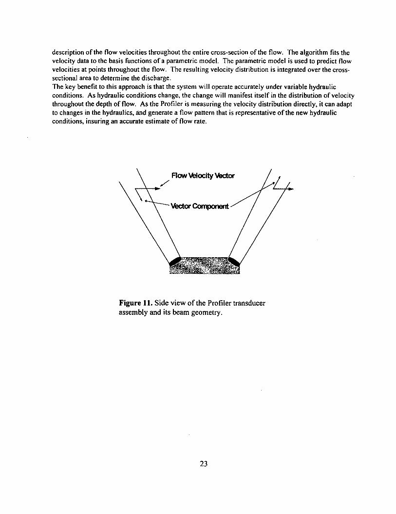
description of the flow velocities throughout the entire cross-section of the flow. The algorithm fits the velocity data to the basis functions of a parametric model. The parametric model is used to predict flow velocities at points throughout the flow. The resulting velocity distribution is integrated over the cross­sectional area to determine the discharge. The key benefit to this approach is that the system will operate accurately under variable hydraulic conditions. As hydraulic conditions change, the change will manifest itself in the distribution ofvelocity throughout the depth of flow. As the Profiler is measuring the velocity distribution directly, it can adapt to changes in the hydraulics, and generate a flow pattern that is representative of the new hydraulic conditions, insuring an accurate estimate of flow rate.

Flow Velocity Vector /

..---+-....

Figure 11. Side view of the Profiler transducer assembly and its beam geometry.

23