Embed Size (px)
Citation preview

Paul Cheshire and Christian A.L. HilberOffice space supply restrictions in Britain: the political economy of market revenge Article (Accepted version) (Refereed) Original citation: Cheshire, Paul and Hilber, Christian A.L. (2008) Office space supply restrictions in Britain: the political economy of market revenge. Economic journal, 118 (529). F185-F221. ISSN 0013-0133 DOI: 10.1111/j.1468-0297.2008.02149.x The definitive version is available at: http://onlinelibrary.wiley.com. © 2008 The authors; published by Wiley-Blackwell on behalf of the Royal Economic Society This version available at: http://eprints.lse.ac.uk/4372/Available in LSE Research Online: February 2011 LSE has developed LSE Research Online so that users may access research output of the School. Copyright © and Moral Rights for the papers on this site are retained by the individual authors and/or other copyright owners. Users may download and/or print one copy of any article(s) in LSE Research Online to facilitate their private study or for non-commercial research. You may not engage in further distribution of the material or use it for any profit-making activities or any commercial gain. You may freely distribute the URL (http://eprints.lse.ac.uk) of the LSE Research Online website. This document is the author’s final manuscript accepted version of the journal article, incorporating any revisions agreed during the peer review process. Some differences between this version and the published version may remain. You are advised to consult the publisher’s version if you wish to cite from it.
Office space supply restrictions in Britain: the political economy of market revenge
Office Space Supply Restrictions in Britain:
The Political Economy of Market Revenge
Paul C. Cheshire and Christian A. L. Hilber
This Version: 15 February 2008
Corresponding author: Paul Cheshire
Professor Paul Cheshire, Dr Christian Hilber
London School of Economics
Department of Geography & Environment
Houghton St
London WC2A 2AE

Office space supply restrictions in Britain: the political economy of market revenge
Office Space Supply Restrictions in Britain:
The Political Economy of Market Revenge
Abstract
Office space in Britain is the most expensive in the world and regulatory constraints are the
obvious explanation. We estimate the ‘regulatory tax’ for 14 British and 8 continental
European office locations. The values for Britain are orders of magnitude greater than any
elsewhere. Exploiting panel data, we provide strong support for our hypothesis that the
regulatory tax varies according to local prosperity and its responsiveness to this depends on
whether an area is controlled by business interests or residents. Our results also imply that
the cost to office occupiers of the 1990 conversion of commercial property taxes from a local
to a national basis – transparently removing any fiscal incentive to local communities to
permit development – exceeded any plausible rise in property taxes.
JEL classification: H3, J6, Q15, R52.
Keywords: Land use regulation, regulatory costs, business taxation, office markets.

Office space supply restrictions in Britain: the political economy of market revenge
1
1 Introduction: The Problem in an International Perspective1
The cost of constructing a m2 of office space in Birmingham, England, in 2004 was
approximately half that in Manhattan.2 This is not very surprising since Birmingham is a
struggling, medium sized city on the flat plains of the British Midlands and Manhattan is big,
topographically constrained, prosperous and highly dynamic. If we were looking for an
American equivalent to Birmingham, maybe, St Louis, Missouri would pop up. When we
couple the cost of construction with the costs of occupation of that same m2, however, we do
get a shock. In the same year, the total occupation costs per m2 were 44% higher in
Birmingham than they were in Manhattan (KingSturge, 2004). Something very odd must be
going on. The obvious anomaly is the intensity and restrictiveness of land use controls in the
UK and this paper sets out to investigate the economic costs of these restrictions and what
drives them.
In the past few years US urban economists have become interested in the analysis of land use
regulation and concerned about increasing regulatory restrictions influencing the supply and
costs of housing3 and perhaps sorting between cities4. Glaeser et al (2005) for example
conclude that regulatory restrictions increase housing prices in the most tightly constrained
metro areas by some 50% and by considerably more in Manhattan. This is potentially of
concern because not only is the effective ‗tax‘ substantial but it has been rising over time.
However, no researcher has yet reported a significant effect of regulatory constraint on the
costs of commercial space in the US. This is no great surprise given the fiscal incentives to
local communities to allow commercial development.
The situation in the UK, however, is several orders of magnitude more restricted. This is
partly because land use regulation in the UK takes the form of universal growth constraints:
and growth constraints applied not just to the total area of urban land take for each city but
individually to each category of land use within each city. So urban ‗envelopes‘ are fixed by
growth boundaries but within these envelopes the areas of land available for retail, offices,
warehouses and industry are all tightly controlled. Although not entirely inflexible,
Greenbelts surrounding cities have been more or less sacrosanct since they were established,
out of town retail is effectively prohibited5, and local planning authorities have been
extremely reluctant to expand the area zoned for commercial space. There are, moreover, a
raft of preservation designations and height controls on buildings. The present pattern of
regulation was essentially set in aspic in 1947 so has been in place for two generations.
1 We thank John Clapp, Robin Goodchild, Colin Lizieri, John Muellbauer, John Quigley, Tsur Somerville and
Sotiris Tsolacos for helpful comments and suggestions. We are grateful to Robin Goodchild, courtesy of Jones
Lang LaSalle, Peter Damesick from UK CB Richard Ellis and Simon Rawlinson from Davis Langdon for kindly
providing essential data. Thanks also to an anonymous referee and the editor of this journal for helpful
comments. Gerard Dericks provided excellent research assistance. The remaining errors are the sole
responsibility of the authors. 2 This uses the ratio of Birmingham office construction costs to those in London from Davis Langdon (see
Section 3 of this paper), the ratio of Davis Langdon‘s London construction cost estimates to those from Gardiner
and Theobald to apply to Gardiner and Theobald‘s construction cost data for New York offices to estimate
figures on a comparable basis for both Birmingham and New York. 3 See, for example, Brueckner (2000); Evenson and Wheaton (2003); Glaeser and Gyourko (2003); Glaeser et al
(2005); Mayer and Somerville (2000); Mayo and Sheppard (2001); Phillips and Goodstein (2000); or Song and
Knaap (2003). 4 See Gyouko et al (2005).
5 On two different grounds: to maintain the economic strength of city centres and to reduce car use. Whether
either objective is actually served by this policy and, in so far as it is, at what cost – is unclear.
Office space supply restrictions in Britain: the political economy of market revenge
2
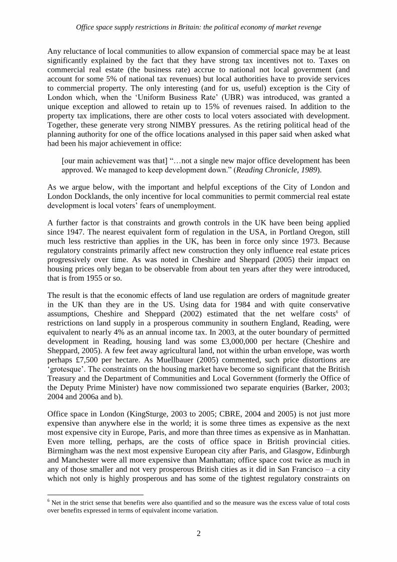
Any reluctance of local communities to allow expansion of commercial space may be at least
significantly explained by the fact that they have strong tax incentives not to. Taxes on
commercial real estate (the business rate) accrue to national not local government (and
account for some 5% of national tax revenues) but local authorities have to provide services
to commercial property. The only interesting (and for us, useful) exception is the City of
London which, when the ‗Uniform Business Rate‘ (UBR) was introduced, was granted a
unique exception and allowed to retain up to 15% of revenues raised. In addition to the
property tax implications, there are other costs to local voters associated with development.
Together, these generate very strong NIMBY pressures. As the retiring political head of the
planning authority for one of the office locations analysed in this paper said when asked what
had been his major achievement in office:
[our main achievement was that] ―…not a single new major office development has been
approved. We managed to keep development down.‖ (Reading Chronicle, 1989).
As we argue below, with the important and helpful exceptions of the City of London and
London Docklands, the only incentive for local communities to permit commercial real estate
development is local voters‘ fears of unemployment.
A further factor is that constraints and growth controls in the UK have been being applied
since 1947. The nearest equivalent form of regulation in the USA, in Portland Oregon, still
much less restrictive than applies in the UK, has been in force only since 1973. Because
regulatory constraints primarily affect new construction they only influence real estate prices
progressively over time. As was noted in Cheshire and Sheppard (2005) their impact on
housing prices only began to be observable from about ten years after they were introduced,
that is from 1955 or so.
The result is that the economic effects of land use regulation are orders of magnitude greater
in the UK than they are in the US. Using data for 1984 and with quite conservative
assumptions, Cheshire and Sheppard (2002) estimated that the net welfare costs6 of
restrictions on land supply in a prosperous community in southern England, Reading, were
equivalent to nearly 4% as an annual income tax. In 2003, at the outer boundary of permitted
development in Reading, housing land was some £3,000,000 per hectare (Cheshire and
Sheppard, 2005). A few feet away agricultural land, not within the urban envelope, was worth
perhaps £7,500 per hectare. As Muellbauer (2005) commented, such price distortions are
‗grotesque‘. The constraints on the housing market have become so significant that the British
Treasury and the Department of Communities and Local Government (formerly the Office of
the Deputy Prime Minister) have now commissioned two separate enquiries (Barker, 2003;
2004 and 2006a and b).
Office space in London (KingSturge, 2003 to 2005; CBRE, 2004 and 2005) is not just more
expensive than anywhere else in the world; it is some three times as expensive as the next
most expensive city in Europe, Paris, and more than three times as expensive as in Manhattan.
Even more telling, perhaps, are the costs of office space in British provincial cities.
Birmingham was the next most expensive European city after Paris, and Glasgow, Edinburgh
and Manchester were all more expensive than Manhattan; office space cost twice as much in
any of those smaller and not very prosperous British cities as it did in San Francisco – a city
which not only is highly prosperous and has some of the tightest regulatory constraints on
6 Net in the strict sense that benefits were also quantified and so the measure was the excess value of total costs
over benefits expressed in terms of equivalent income variation.

Office space supply restrictions in Britain: the political economy of market revenge
3
housing in the US but also has topographical constraints on land supply. Office space in
Birmingham cost 124% more than in fast growing, twice as big and land strapped Singapore.
To date there has been rigorous quantification of the economic effects of land use constraints
on the UK housing sector but not for any category of commercial property. The purpose of
this paper is to address this gap in our knowledge and investigate the costs of land use
regulation for commercial property in the UK in a rather more rigorous way than is possible
when just comparing the rent and occupation costs.
An obvious problem in analysing the economic impacts of land use planning is identifying
exactly what element in total occupation costs – the cost of space to economic agents - may
reasonably be attributed to ‗planning‘ restrictions. This is because i) such restrictions take
many forms over and beyond restricting the supply of land or space; and ii) it is difficult to
offset for the normal factors such as city size etc, that urban economic theory tells one should
be expected to influence the price of land and space. Furthermore, if we want to estimate the
economic impact of any measured increase in space costs resulting from regulation, we would
need to go a second step – not included in this research. We should estimate the impact on
output, employment and incomes generated by the increase in space costs produced by
regulatory constraints. Then offset those costs against any benefits regulation produced.
In the context of the residential sector, a theoretically rigorous methodology was set out in
Cheshire and Sheppard (2002) for estimating both the gross and the net costs of regulatory
restrictions on the supply of residential land and so the net welfare cost these had. This,
however, is demanding on data and research time and depends on being able to explicitly
identify and estimate the economic impacts of the goods/amenities generated by planning, the
impact of regulation on supply and the indirect utility functions of residents/citizens. Even if
it were not so data intensive, it is not clear such a methodology could be adapted to estimating
the economic and welfare impacts of regulation of the supply of non-residential property
because of the difficulty of estimating the relevant production function.
We estimate here, just the first of these elements: a measure of the total cost of regulatory
constraints on the price of office space expressed as a ‗tax‘ – that is as a percentage of
construction costs. To do this we adapt the methodology first developed and applied to the
Manhattan condominium market by Glaeser et al (2005). The value of this measure and its
interpretation is the subject of section 2 of this paper. The Glaeser et al (2005) methodology
has the considerable attraction that it is intellectually coherent, resting on established
microeconomic theory, and it is not too demanding with respect to data and estimation
techniques. Its downside is that it is a ‗black box‘ number in that it does not differentiate
between costs that are imposed by different aspects of regulation and may miss certain types
of cost that regulation imposes. It is an aggregate measure of the gross cost of regulatory
constraints limiting the height and floor area of buildings and – more indirectly – the supply
of land for the use in question. So it reflects the costs of restrictions on land supply, space by
plot ratios or height restrictions, or common forms of conservation designation. It does not,
however, capture costs imposed by compliance complexity or delays in decision making. In
addition, it only gives a ‗cost‘ not a net welfare or net impact on output measure. As is well
known, there are measurable benefits from some aspects of regulation and, since space is
substitutable to a degree in both production and consumption, the effects on output or welfare
can only be estimated if both the benefits and the extent of substitutability are known. So the
regulatory tax estimates are a lower bound estimate of a gross cost of land use regulation in
any location.

Office space supply restrictions in Britain: the political economy of market revenge
4
Glaeser et al (2005) report their results for Manhattan apartments as a price to construction
cost ratio (rather than as a quasi-tax rate; regulatory tax to marginal construction cost). For the
most recent year they had data for, 2002, this ratio was 2.07. In our tax-rate measure and
subject to the caveat that we are explicitly measuring from observed marginal construction
costs, this would translate to a value of 1.07. They also investigated other data which
suggested that the value of the regulatory tax on housing was higher in some West Coast
urban areas, such as the Bay Area and Los Angeles, than it was in the New York urban area
as a whole (it was much higher in Manhattan itself than it was in the New York metro area)
although it was still substantial in the New York area. However, in 10 of the 21 urban areas
investigated there was no measurable impact of regulation on house prices. Nor was there any
indication of a significant ‗regulatory tax‘ on office property in Manhattan. This provides
some standard against which to evaluate the results for office property in the British cities
reported below.
2 An Interpretation of the Regulatory Tax (RT) as a Measure of the
Costs of Restrictions
The key idea of the Regulatory Tax (RT) approach is simple; in a world with competition
among property developers and free market entry and exit, price will equal (minimum)
average cost since this includes ‗normal‘ profit. We would argue that competition between
developers and free entry are reasonable assumptions both because of the low costs of entry to
small scale development, such as converting a single building to office use, and the
international nature of the development industry. In Britain the best known example of
international entry might be Olympia and York, the Canadian developers of Canary Wharf,
but most provincial office locations have examples of buildings developed by Japanese,
German, Dutch or Swedish developers.
Marginal construction costs rise with building height, so in the absence of restrictions on
heights, buildings should rise to a point where the marginal cost of adding an additional floor
equals its market price. If building higher is less profitable per m2 than building over a greater
area, we still should expect the marginal cost of an extra floor to be equal to price: buildings
would just be lower on average but the overall urban land take would be greater. Bertaud and
Brueckner (2005) demonstrate the formal equivalence of height restrictions compared to land
supply restrictions. Any gap between the observed market price and the marginal construction
cost can be interpreted, therefore, as a ‗regulatory tax‘ – the additional cost of space resulting
– in aggregate – from the system of regulation in that particular market. If the sales price of an
additional floor of office space exceeded the marginal cost of building this additional floor
then developers would have an arbitrage opportunity. The difference between the price of
floor space and its cost of construction must be due to some form of regulation.
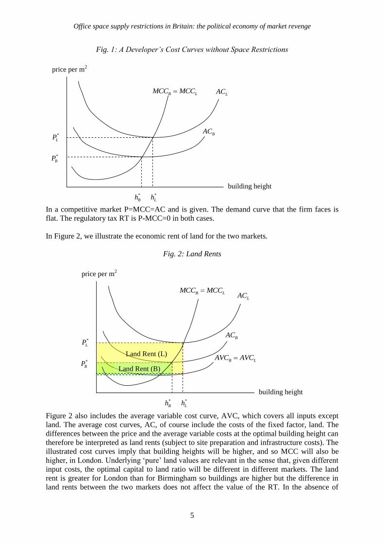
This is illustrated in Figure 1 which depicts the cost curves of representative competitive
developers in (by assumption) two unregulated markets; one relatively prosperous and
‗attractive‘ office market, say, London (L) and one less prosperous and ‗attractive‘ market,
say, Birmingham (B). For illustrative convenience, we assume that the marginal construction
cost curve (MCC) is identical in both markets implying that wages, materials and other
variable costs do not vary regionally. We also assume – quite reasonably – that buildings of a
given type have an optimal floor plan to height ratio (given the price of land). To make the
diagram easier to follow we intentionally exaggerate the extent to which marginal
construction costs rise with building height.
Office space supply restrictions in Britain: the political economy of market revenge
5
Fig. 1: A Developer’s Cost Curves without Space Restrictions
LAC
*
LP
*
BP
BAC
B LMCC MCC
building height
price per m2
*
Bh *
Lh
In a competitive market P=MCC=AC and is given. The demand curve that the firm faces is
flat. The regulatory tax RT is P-MCC=0 in both cases.
In Figure 2, we illustrate the economic rent of land for the two markets.
Fig. 2: Land Rents
B LMCC MCC
*
Bh
*
BP B LAVC AVC
LAC
*
LP
BAC
building height
price per m2
Land Rent (L)
Land Rent (B)
*
Lh
Figure 2 also includes the average variable cost curve, AVC, which covers all inputs except
land. The average cost curves, AC, of course include the costs of the fixed factor, land. The
differences between the price and the average variable costs at the optimal building height can
therefore be interpreted as land rents (subject to site preparation and infrastructure costs). The
illustrated cost curves imply that building heights will be higher, and so MCC will also be
higher, in London. Underlying ‗pure‘ land values are relevant in the sense that, given different
input costs, the optimal capital to land ratio will be different in different markets. The land
rent is greater for London than for Birmingham so buildings are higher but the difference in
land rents between the two markets does not affect the value of the RT. In the absence of
Office space supply restrictions in Britain: the political economy of market revenge
6
restrictions, RT will be zero. This, indeed, is one of the attractions of the RT measure. Since
land costs are an element in fixed costs, they never affect the measured RT. Since land costs
are difficult to measure and it is considerably more difficult still to estimate any impact of
land use regulation on the cost of land, the RT measure of the costs of regulation entirely
avoids a difficult problem.
We can think about this in more detail by considering two cases. Case F is the unregulated
situation while Case R is the regulated one.
Case F: Suppose we have an unregulated world with a competitive development and office
market and the cost of an additional floor rises with building height: then building heights rise
until, per m2 Marginal Cost of Construction (MCC)=Marginal Revenue (MR)=Average Cost
(AC)=Price (P)=Average Revenue (AR). In such a market, therefore, the price per m2
includes all costs for a given building: construction + land + normal profit. Suppose we then
add a hypothetical additional floor. The MCC per m2
is higher for this additional floor than for
the existing highest floor but price is not. The ‗land‘ is already paid for in the existing
building, part of fixed costs and included in AC. There is, then, no appreciable RT.
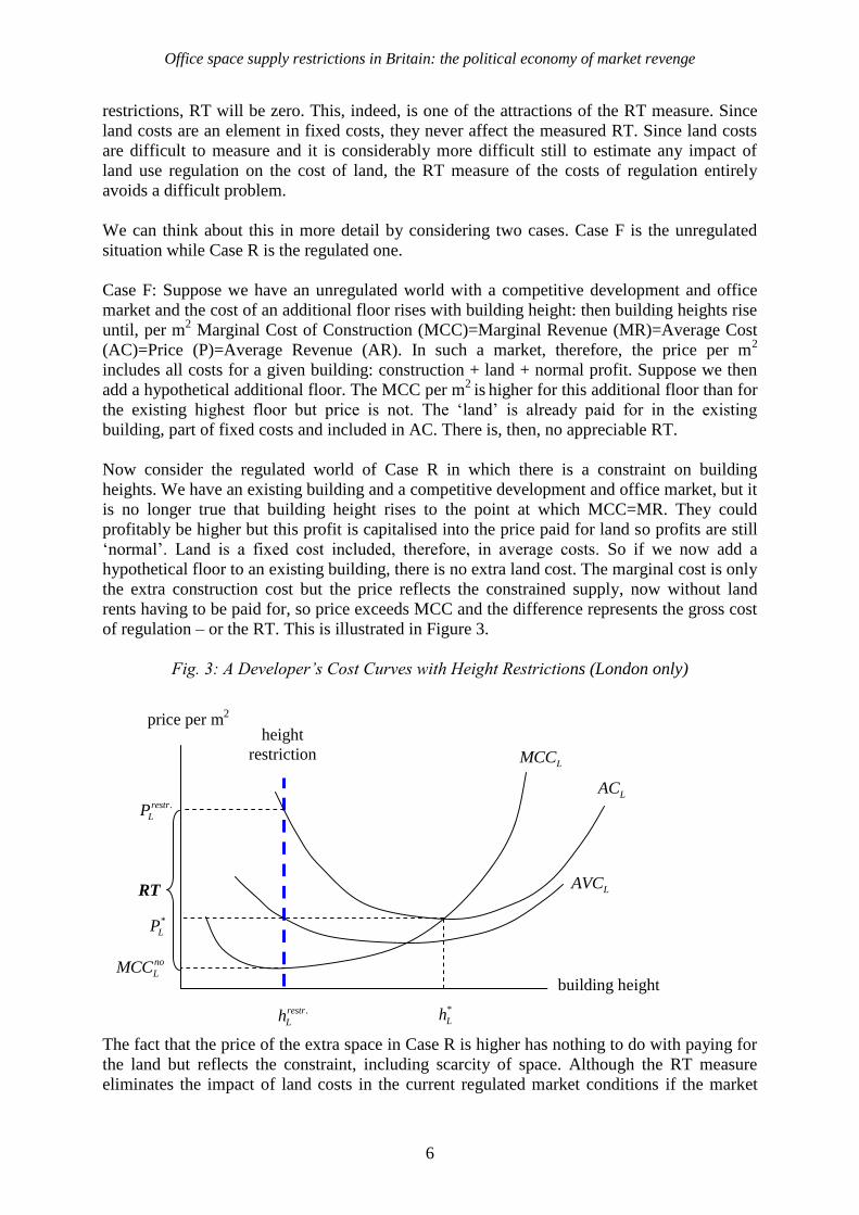
Now consider the regulated world of Case R in which there is a constraint on building
heights. We have an existing building and a competitive development and office market, but it
is no longer true that building height rises to the point at which MCC=MR. They could
profitably be higher but this profit is capitalised into the price paid for land so profits are still
‗normal‘. Land is a fixed cost included, therefore, in average costs. So if we now add a
hypothetical floor to an existing building, there is no extra land cost. The marginal cost is only
the extra construction cost but the price reflects the constrained supply, now without land
rents having to be paid for, so price exceeds MCC and the difference represents the gross cost
of regulation – or the RT. This is illustrated in Figure 3.
Fig. 3: A Developer’s Cost Curves with Height Restrictions (London only)
*
LP
.restr
LP
no
LMCC
height
restriction
LAVC
LAC
LMCC
building height
price per m2
RT
*
Lh .restr
Lh
The fact that the price of the extra space in Case R is higher has nothing to do with paying for
the land but reflects the constraint, including scarcity of space. Although the RT measure
eliminates the impact of land costs in the current regulated market conditions if the market

Office space supply restrictions in Britain: the political economy of market revenge
7
were unregulated, land costs per m2 would be lower: so the observed MCC in a regulated
market is likely to differ from that in an unregulated market.
Other forms of planning imposed constraint are possible, however. Plot ratio constraints (in
the USA floor area ratios) which determine the maximum floor space relative to the size of
the site are common. Again consider first a world without constraints. In the absence of any
regulations the developer would choose an optimal floor plan and corresponding optimal
height such that MCC=AC=P. Moreover, the developer could ignore negative externalities,
such as restricted views the building causes to its neighbours, so would have an incentive to
choose the site just big enough to accommodate the floor plan subject to user preferences and
impacts of plot ratios on the productivity of the building.
Fig. 4: A Developer’s Cost Curves with Plot Ratio Constraints (London only)
no plr
LAC
LMCC
floor space
price per m2
. incr site areaRT
plr
LAC
reduce heightRT
*
Ls plr
Ls
With the plot ratio constraint, however, in order to build the identical property, the developer
would have to either (a) increase the size of the site, keeping the floor plan constant or (b)
reduce the height of the building, again keeping the floor plan constant. Consider case (a)
first. The additional land needed to reduce the plot ratio to reach the threshold level adds fixed
cost, so increases AC, but has no effect on MCC. This effect is illustrated in Figure 4. The RT
in this case is the difference between plrAC and MCC at the original optimal floor space *s .
Alternatively (case b), the developer could reduce the height of the building until the
corresponding floor space reduction (from *s to plrs ) is sufficient to conform to the plot ratio
constraint. This case is equivalent to the height restriction constraint described above. In this
case the RT would be the difference between no plrAC and MCC at the point plrs . The
observed RTs in the two cases will not typically be the same but they will both be strongly
positively correlated with the degree to which the plot ratio is binding.7 Of course, the
7 In fact it can be easily demonstrated for the case of linear MCC curves and land as the only fixed cost that both
RT measures increase with the rigidness of the plot ratio constraint. The RT associated with a height reduction is
always larger than the RT associated with a proportional increase in the site area. For example, if the optimal
floor space needs to be reduced in half to comply with the plot ratio constraint, then the RT associated with the
site increase is exactly 2/3 of the proportional height reduction. The relative difference between the two RT
measures decreases with increasing rigidness of the constraint. In the limit, with the rigidness of the plot ratio
constraint becoming extremely binding, the two RT measures become identical.

Office space supply restrictions in Britain: the political economy of market revenge
8
developer has a third option, to reduce the floor plan itself, keeping the site area and building
height constant. In Figure 4 with floor space on the x-axis this is equivalent to the height-
reduction case.
In reality, however, the two cases are not equivalent since at some point the cost per floor
starts to rise exponentially with the number of floors. To illustrate this argument, consider the
following case: To provide 36,000 m2 of space (a large office building) with a floor plan of
1,200 m2 would imply a 30 storey building and so a height of, say, 100 metres: to get the
same space with a floor plan of only 25m2 per floor would imply 1,440 stories – a building
some 4.75 kilometres high. Clearly, apart from issues of technical feasibility, at some extreme
height the cost of adding an additional storey will become astronomically high.
Now consider another extreme of hypothetical regulation: suppose that there are no
constraints on building or land availability at all, but stringent compliance costs related to,
say, permits, but such costs are a function only of individual buildings so are a fixed cost.
Once the compliance process has been completed, the agreed building can be constructed with
no further compliance costs at all. In such a case, the costs of compliance will appear as a
fixed cost and, if the results related to the incidence of Impact Fees are applicable (Ihlanfeldt
and Shaughnessy, 2004) will be fully (negatively) capitalised into land prices. Thus, there
could be no impact on marginal construction costs or on the price of space. There will be a
deadweight loss, but this loss will fall uniquely on the price of land although given that the
profitability of transferring land from agricultural to urban use will be reduced, it could
reduce the overall supply of urban land and so have some affect on space costs.
For illustrative purposes, the analysis above has been in a partial equilibrium setting from the
perspective of a single developer or building. However, in practice not all regulatory
constraints are as simple as this. In Britain there are simultaneous restrictions imposed on plot
ratios, building heights and on the total area of land on which, in any city, it is permitted to
build offices as well as compliance costs. In these circumstances in any city in which there is
a strong demand for office space, there will be a binding constraint on total space availability
driving up both the price of space and the price of land with permission to develop. It will still
be clear, however, that AC (which includes the costs of land) will be above MCC so the RT
measure will reflect the overall space constraint in the market.
What these examples suggest is that the relationship between measured RT and the actual
gross costs of regulation (if these could be measured exactly) is, in principle, a variable one
and will depend on the precise form the regulatory constraints take. So long as at least an
element of the regulatory constraints takes the form of restrictions on the height of buildings
and plot ratios, however, the measured RT will be strongly and positively correlated with the
actual gross costs of regulatory constraints. The RT measure, however, will likely be a lower
bound estimate of the gross costs because, for example, some of the regulatory constraints
may relate to compliance costs or costs of delay.
Need this concern us particularly in the case of British offices? Restrictions on building
heights take several forms but are applied in all British markets. In the City of London, for
example, no less than eight separate ‗view corridors‘ of St Paul‘s cathedral (both foreground
and background) are protected from building above some 55 metres and five ‗view corridors‘
of the Monument are similarly protected as are four street blocks around the Monument (City
of London, 1991). There are, in addition, extensive ‗Conservation Areas‘ within which very
limited changes to the external appearance of buildings is possible – obviously including

Office space supply restrictions in Britain: the political economy of market revenge
9
height - and, throughout the City – as in all British cities – there are ‗plot ratios‘ controlling
the total size of buildings relative to the size of the site. These were set at 5.1:1 in the City
(City of London, 1991, para. 16.42). There are, in addition, other regulations affecting the
design of buildings which limit height and space within them. Planning policies in London‘s
West End are substantially more restrictive than those in the City, since very large areas –
most of Mayfair and Belgravia – are designated Conservation Areas where it is not possible to
build higher than the existing structure and changes to the external appearance of buildings
are prohibited. If the building is individually listed – as a high proportion of buildings in
London‘s West End are – then even internal alterations are prohibited. Such historic
conservation regulations undoubtedly generate amenity values, not included in a measure of
RT.
In summary, then, the RT measure of the gross costs of regulatory constraints on buildings is
something of a black box in that it will incorporate the cost of restrictions on the supply of
land for the use in question and restrictions on building heights. These may arise from various
sources but are imposed in all British office locations by ‗plot ratio‘ controls. Since land use
planning is a national system in Britain it seems likely that compliance costs and costs of
delay do not vary significantly across locations but such costs will not be fully captured in the
RT measure and may not be captured at all. So we can conclude that estimated RT values will
be strongly and positively correlated with actual gross costs of regulatory constraints but in
absolute terms may be lower bound estimates.
3 Data and methodology
Here we discuss the data used to estimate regulatory tax values which as noted above, we
express as a rate relative to marginal construction costs. The total unemployment rate and
service employment growth rate data used in the subsequent analysis are discussed in Section
6. To estimate the RT we need ‗price‘ and ‗marginal construction cost‘ data. Our empirical
analysis builds on the best available data for the British office market and a number of
continental European cities. After careful and detailed discussion to agree how best to
measure marginal costs of construction (i.e., the estimated cost of adding an additional
hypothetical floor to an existing building) Davis Langdon estimated time-series data for the
agreed definitions by market (per square metre). Davis Langdon is the leading UK producer
of construction cost data for the building industry and produces the Spon Handbooks used by
quantity surveyors and architects (Davis Langdon, 2005). A detailed description of the
methodology Davis Langdon used to derive the marginal cost of construction is explained in
Cheshire and Hilber (2007). Gardiner and Theobald (2006) – Davis Langdon‘s major
competitor – provide (average) construction cost data for our sample of continental European
cities. Unfortunately, comparable time-series data on the market price of office space, in the
sense of capital values, is not readily available; only data on rents, yields, vacancies and rent
free periods can be obtained. CB Richard Ellis (CBRE) the largest property consultancy in the
UK, provided the relevant data for British markets. Similar data (although estimated on a
different basis) were also provided by Jones Lang LaSalle (JLL) for a number of our British
locations and all the continental European ones we report estimates for in Table 2. We used
the common British locations to make the best adjustment we could to a comparable basis.
Only rental not capital values are available because office buildings are treated as income
producing assets that are typically leased floor by floor. We therefore need to impute the
market price per m2 of an additional floor of office space (the ‗capitalised value‘) using the
available information on rents, yields, rent-free periods and vacancy rates. The estimation
Office space supply restrictions in Britain: the political economy of market revenge
10
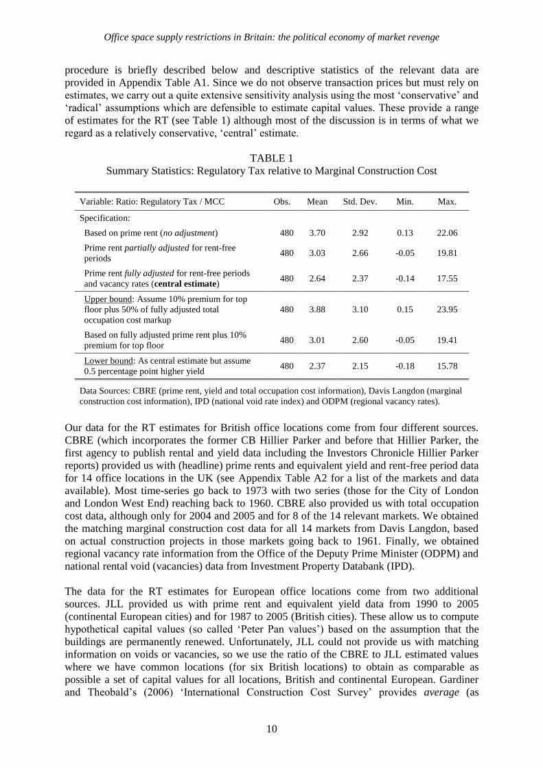
procedure is briefly described below and descriptive statistics of the relevant data are
provided in Appendix Table A1. Since we do not observe transaction prices but must rely on
estimates, we carry out a quite extensive sensitivity analysis using the most ‗conservative‘ and
‗radical‘ assumptions which are defensible to estimate capital values. These provide a range
of estimates for the RT (see Table 1) although most of the discussion is in terms of what we
regard as a relatively conservative, ‗central‘ estimate.
TABLE 1
Summary Statistics: Regulatory Tax relative to Marginal Construction Cost
Variable: Ratio: Regulatory Tax / MCC Obs. Mean Std. Dev. Min. Max.
Specification:
Based on prime rent (no adjustment) 480 3.70 2.92 0.13 22.06
Prime rent partially adjusted for rent-free
periods 480 3.03 2.66 -0.05 19.81
Prime rent fully adjusted for rent-free periods
and vacancy rates (central estimate) 480 2.64 2.37 -0.14 17.55
Upper bound: Assume 10% premium for top
floor plus 50% of fully adjusted total
occupation cost markup
480 3.88 3.10 0.15 23.95
Based on fully adjusted prime rent plus 10%
premium for top floor 480 3.01 2.60 -0.05 19.41
Lower bound: As central estimate but assume
0.5 percentage point higher yield 480 2.37 2.15 -0.18 15.78
Data Sources: CBRE (prime rent, yield and total occupation cost information), Davis Langdon (marginal
construction cost information), IPD (national void rate index) and ODPM (regional vacancy rates).
Our data for the RT estimates for British office locations come from four different sources.
CBRE (which incorporates the former CB Hillier Parker and before that Hillier Parker, the
first agency to publish rental and yield data including the Investors Chronicle Hillier Parker
reports) provided us with (headline) prime rents and equivalent yield and rent-free period data
for 14 office locations in the UK (see Appendix Table A2 for a list of the markets and data
available). Most time-series go back to 1973 with two series (those for the City of London
and London West End) reaching back to 1960. CBRE also provided us with total occupation
cost data, although only for 2004 and 2005 and for 8 of the 14 relevant markets. We obtained
the matching marginal construction cost data for all 14 markets from Davis Langdon, based
on actual construction projects in those markets going back to 1961. Finally, we obtained
regional vacancy rate information from the Office of the Deputy Prime Minister (ODPM) and
national rental void (vacancies) data from Investment Property Databank (IPD).
The data for the RT estimates for European office locations come from two additional
sources. JLL provided us with prime rent and equivalent yield data from 1990 to 2005
(continental European cities) and for 1987 to 2005 (British cities). These allow us to compute
hypothetical capital values (so called ‗Peter Pan values‘) based on the assumption that the
buildings are permanently renewed. Unfortunately, JLL could not provide us with matching
information on voids or vacancies, so we use the ratio of the CBRE to JLL estimated values
where we have common locations (for six British locations) to obtain as comparable as
possible a set of capital values for all locations, British and continental European. Gardiner
and Theobald‘s (2006) ‗International Construction Cost Survey‘ provides average (as

Office space supply restrictions in Britain: the political economy of market revenge
11
opposed to marginal) construction cost data back to 1999 so we can estimate RT values from
1999 to 2005. We use the ratio of marginal to average construction costs from Davis Langdon
and Gardiner and Theobald for the two markets (the City of London and London West End)
for which both sets of data are available to estimate the hypothetical marginal cost of
construction for the continental European office locations.8
Imputing Missing Values
Our raw data come in different time-intervals. The prime rent data, for example, are quarterly
for the City of London and London‘s West End back to 1960; however, they are quarterly,
monthly, half-annually and annually for the other 12 markets, in all but three cases, back to
1973. Similarly, the yield data come in various time intervals. The construction cost data are
annual. Hence, in order to make our data comparable, we use annual numbers when available
and compute annual numbers when not.
Even though we use annualised data, we still have missing values for a number of variables
and markets. For example, we only obtained rent-free period data for two markets (the City
of London and London‘s West End) and only between 1993 and 2006. For the remaining
years and other markets we need to impute the rent-free periods using the available data (see
Cheshire and Hilber, 2007, for details). Similarly, we need to impute equivalent yields prior to
1972 using the available data (again see Cheshire and Hilber, 2007, for details). The imputed
values obviously introduce an additional degree of uncertainty into estimates prior to 1972.
We also have to impute vacancy rates from relatively short time-series of regional data from
ODPM and longer time-series data from IPD; details are again available in Cheshire and
Hilber (2007). Imputing values of yields could, we believe, have a significant impact on the
final estimates of RT. So we should be very cautious with respect to any interpretation of
estimated values of the RT prior to 1972. The absolute differences to estimates resulting from
any plausible alternative values of rent free periods and vacancy rates are, however,
comparatively small. We are confident, therefore, that while the need to impute values for
such data is not entirely satisfactory, the additional margin of error it may introduce into the
estimates is small in relative terms.
We have to impute missing rental values using national rent-index data from Hillier Parker
(today CBRE). The Hillier Parker ICHP national rent-index data is available back to 1965 but
only for three years. This does allow us to impute missing rental values between 1965 and
1972 but for missing years, we assume a linear trend.
Finally, we impute total occupation cost by assuming a constant scaling factor to fully
adjusted prime rents using the ratio: average of the total occupation cost for each market in
2004 and 2005 divided by fully adjusted prime rent. We can match prime rent and total
occupation costs for 8 of the 14 markets. For the remaining 6 markets we assume the ratio of
the geographically closest market for which data are available.
8 This approach is imperfect as it is unlikely, as an anonymous referee pointed out, that the relationship between
average construction cost (ACC) and marginal construction cost (MCC) is constant across markets and over
time. In fact, one can show that to the extent that continental European markets have lower ACC and MCC and
are less strongly regulated (compared to the two London markets) we will overestimate the RT for the low cost
and less rigid markets, suggesting that the true RT for the least regulated market (Brussels) might be even closer
to zero than we estimate. Similarly, to the extent that the true RT in any continental European market is
decreasing (increasing) over time, our approach will tend to understate the change. Observations for the City of
London for which we have the two alternative estimates of the RT appear to confirm the predicted bias; when we
use the actual MCC we estimate quite a steep decline in the RT between 1999 and 2005. When we have to rely
on adjusted ACC information we find a much less steep decline.

Office space supply restrictions in Britain: the political economy of market revenge
12
Our goal is to estimate, as accurately as possible, the magnitude of the RT over time for the
14 local office markets. The RT (expressed as a tax rate) can be formulated as:
1jt jt jt
jt
jt jt
V MCC VRT = =
MCC MCC
(1)
where Vjt is the market value of an additional square metre of office space in market j at time
period t and where MCCjt is the corresponding marginal construction cost of adding one
square metre of an additional floor.
The market value of a square metre of additional office space is estimated using the
‗Equivalent Yield Model‘, which is probably the most commonly used model to value income
producing property in Britain (see Brown and Matysiak, 2000, for details). According to the
equivalent yield model, the property value can be expressed as:
1
jt jt jt
jt
jtjt jt
jt n
I R IV
y y y
(2)
where jtV is the value of the property (in location j at time period t), jty is the corresponding
equivalent yield, jtR is the so called ‗current rental value‘, jtI is the ‗passing income‘ and jtn
is the number of years to the next rent review.
The equivalent yield is equal to the internal rate of return (IRR) of two cash flow streams (a
stream of ‗passing incomes‘ up to the rent review and then a stream of current rental values,
assumed to be constant, in real terms, in perpetuity). The ‗passing income‘ (which is
expressed in nominal terms) only includes the rents that the tenants ‗pass‘ on to their landlord.
Tenants that are still in their rent-free period or non-rented space do not contribute to the
passing income. Hence, in order to get from the (headline) prime rent to the passing income,
adjustments for rent-free periods and vacancies have to be made as follows:
1 1jt jt
jt jt
Rent Free Period Vacancy Rate in %I Prime Rent
Typical Contract Length 100
. (3)
The ‗current rental value‘ is measured in real terms and is assumed to remain constant in
perpetuity. The capitalised value of the current rental value reflects the reversion value at the
time when the current lease expires.
If we make the reasonable assumption that the current rental value (in real terms) equals the
passing income, then the property value can be expressed as
jt
jt
jt
IV
y . (4)
Using equation (3), the estimated value can finally be expressed as:
Office space supply restrictions in Britain: the political economy of market revenge
13
Rent Free Period Vacancy Rate in %Prime Rent 1 1
Typical Contract Length 100
jt jt
jt
jt
jt
Vy
. (4.1)
The main advantage of using the equivalent yield model to estimate the capitalised value of
office space is that it requires estimates of only two unknown variables – passing income and
the equivalent yield. The equivalent yield can be estimated from comparable properties in the
local market place that have recently been sold.
Although the equivalent yield model is simplistic and obviously has a number of serious
economic shortcomings, it provides surprisingly accurate valuations. This is probably for
some combination of two reasons: First, professional valuers (‗appraisers‘ in the US) are
familiar with subtle changes in the market that will influence the choice of yield; and second,
valuers‘ valuations – based on the equivalent yield model – are the basis for transactions.
Hence, even if a valuation does not reflect the ‗true value‘ of a property (reflecting all future
cash flows discounted at the ‗correct‘ rate), as long as buyers and sellers use the same
valuation model, they will end up agreeing on a (transaction) price that reflects the model‘s
predicted value.
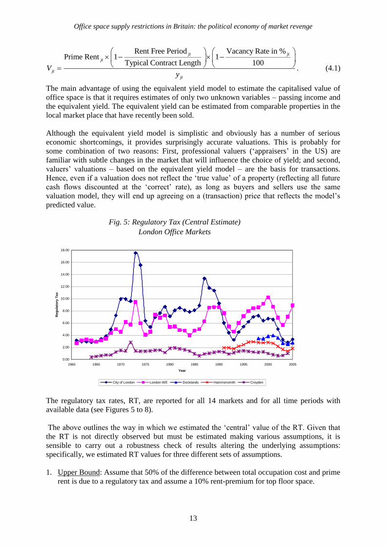
Fig. 5: Regulatory Tax (Central Estimate)
London Office Markets
0.00
2.00
4.00
6.00
8.00
10.00
12.00
14.00
16.00
18.00
1960 1965 1970 1975 1980 1985 1990 1995 2000 2005
Year
Re
gu
lato
ry T
ax
City of London London WE Docklands Hammersmith Croyden
The regulatory tax rates, RT, are reported for all 14 markets and for all time periods with
available data (see Figures 5 to 8).
The above outlines the way in which we estimated the ‗central‘ value of the RT. Given that
the RT is not directly observed but must be estimated making various assumptions, it is
sensible to carry out a robustness check of results altering the underlying assumptions:
specifically, we estimated RT values for three different sets of assumptions.
1. Upper Bound: Assume that 50% of the difference between total occupation cost and prime
rent is due to a regulatory tax and assume a 10% rent-premium for top floor space.
Office space supply restrictions in Britain: the political economy of market revenge
14
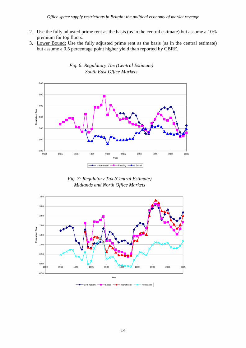
2. Use the fully adjusted prime rent as the basis (as in the central estimate) but assume a 10%
premium for top floors.
3. Lower Bound: Use the fully adjusted prime rent as the basis (as in the central estimate)
but assume a 0.5 percentage point higher yield than reported by CBRE.
Fig. 6: Regulatory Tax (Central Estimate)
South East Office Markets
0.00
1.00
2.00
3.00
4.00
5.00
6.00
1960 1965 1970 1975 1980 1985 1990 1995 2000 2005
Year
Re
gu
lato
ry T
ax
Maidenhead Reading Bristol
Fig. 7: Regulatory Tax (Central Estimate)
Midlands and North Office Markets
-0.50
0.00
0.50
1.00
1.50
2.00
2.50
3.00
3.50
1960 1965 1970 1975 1980 1985 1990 1995 2000 2005
Year
Re
gu
lato
ry T
ax
Birmingham Leeds Manchester Newcastle
Office space supply restrictions in Britain: the political economy of market revenge
15
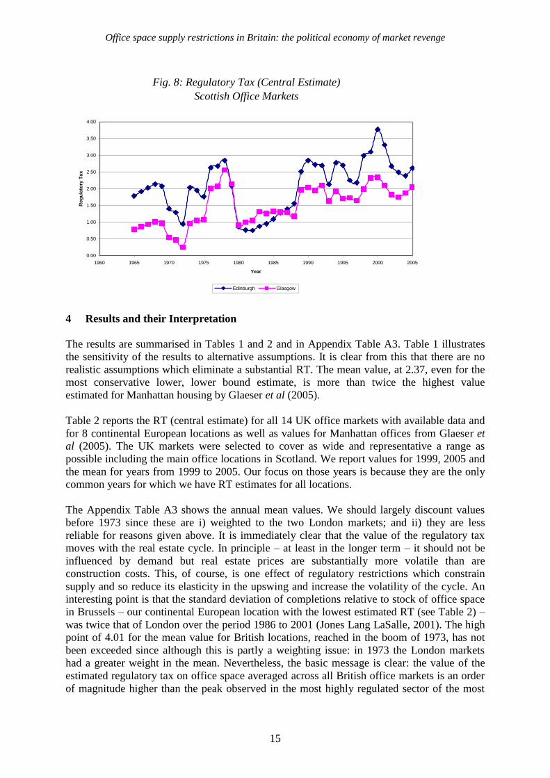
Fig. 8: Regulatory Tax (Central Estimate)
Scottish Office Markets
0.00
0.50
1.00
1.50
2.00
2.50
3.00
3.50
4.00
1960 1965 1970 1975 1980 1985 1990 1995 2000 2005
Year
Re
gu
lato
ry T
ax
Edinburgh Glasgow
4 Results and their Interpretation
The results are summarised in Tables 1 and 2 and in Appendix Table A3. Table 1 illustrates
the sensitivity of the results to alternative assumptions. It is clear from this that there are no
realistic assumptions which eliminate a substantial RT. The mean value, at 2.37, even for the
most conservative lower, lower bound estimate, is more than twice the highest value
estimated for Manhattan housing by Glaeser et al (2005).
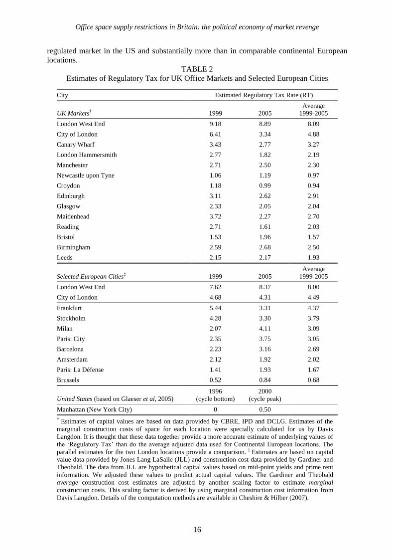
Table 2 reports the RT (central estimate) for all 14 UK office markets with available data and
for 8 continental European locations as well as values for Manhattan offices from Glaeser et
al (2005). The UK markets were selected to cover as wide and representative a range as
possible including the main office locations in Scotland. We report values for 1999, 2005 and
the mean for years from 1999 to 2005. Our focus on those years is because they are the only
common years for which we have RT estimates for all locations.
The Appendix Table A3 shows the annual mean values. We should largely discount values
before 1973 since these are i) weighted to the two London markets; and ii) they are less
reliable for reasons given above. It is immediately clear that the value of the regulatory tax
moves with the real estate cycle. In principle – at least in the longer term – it should not be
influenced by demand but real estate prices are substantially more volatile than are
construction costs. This, of course, is one effect of regulatory restrictions which constrain
supply and so reduce its elasticity in the upswing and increase the volatility of the cycle. An
interesting point is that the standard deviation of completions relative to stock of office space
in Brussels – our continental European location with the lowest estimated RT (see Table 2) –
was twice that of London over the period 1986 to 2001 (Jones Lang LaSalle, 2001). The high
point of 4.01 for the mean value for British locations, reached in the boom of 1973, has not
been exceeded since although this is partly a weighting issue: in 1973 the London markets
had a greater weight in the mean. Nevertheless, the basic message is clear: the value of the
estimated regulatory tax on office space averaged across all British office markets is an order
of magnitude higher than the peak observed in the most highly regulated sector of the most
Office space supply restrictions in Britain: the political economy of market revenge
16
regulated market in the US and substantially more than in comparable continental European
locations.
TABLE 2
Estimates of Regulatory Tax for UK Office Markets and Selected European Cities
City Estimated Regulatory Tax Rate (RT)
UK Markets† 1999 2005
Average
1999-2005
London West End 9.18 8.89 8.09
City of London 6.41 3.34 4.88
Canary Wharf 3.43 2.77 3.27
London Hammersmith 2.77 1.82 2.19
Manchester 2.71 2.50 2.30
Newcastle upon Tyne 1.06 1.19 0.97
Croydon 1.18 0.99 0.94
Edinburgh 3.11 2.62 2.91
Glasgow 2.33 2.05 2.04
Maidenhead 3.72 2.27 2.70
Reading 2.71 1.61 2.03
Bristol 1.53 1.96 1.57
Birmingham 2.59 2.68 2.50
Leeds 2.15 2.17 1.93
Selected European Cities‡ 1999 2005
Average
1999-2005
London West End 7.62 8.37 8.00
City of London 4.68 4.31 4.49
Frankfurt 5.44 3.31 4.37
Stockholm 4.28 3.30 3.79
Milan 2.07 4.11 3.09
Paris: City 2.35 3.75 3.05
Barcelona 2.23 3.16 2.69
Amsterdam 2.12 1.92 2.02
Paris: La Défense 1.41 1.93 1.67
Brussels 0.52 0.84 0.68
United States (based on Glaeser et al, 2005)
1996
(cycle bottom)
2000
(cycle peak)
Manhattan (New York City) 0 0.50
† Estimates of capital values are based on data provided by CBRE, IPD and DCLG. Estimates of the
marginal construction costs of space for each location were specially calculated for us by Davis
Langdon. It is thought that these data together provide a more accurate estimate of underlying values of
the ‗Regulatory Tax‘ than do the average adjusted data used for Continental European locations. The
parallel estimates for the two London locations provide a comparison. ‡
Estimates are based on capital
value data provided by Jones Lang LaSalle (JLL) and construction cost data provided by Gardiner and
Theobald. The data from JLL are hypothetical capital values based on mid-point yields and prime rent
information. We adjusted these values to predict actual capital values. The Gardiner and Theobald
average construction cost estimates are adjusted by another scaling factor to estimate marginal
construction costs. This scaling factor is derived by using marginal construction cost information from
Davis Langdon. Details of the computation methods are available in Cheshire & Hilber (2007).

Office space supply restrictions in Britain: the political economy of market revenge
17
It is more revealing, however, to look at the time series data for the individual markets
reported in Figures 5 to 8 – continuing to focus on the central estimate. The most revealing
point of all is the contrast between the City and West End of London and the role of Canary
Wharf and the development of the Docklands. Until the early 1980s, the City office market
dominated supply and the City was the dominant location, with a quasi-monopolistic control.
It had a highly restrictive planning policy both in terms of height restrictions (which still
endure) and historic designation. Even as late as 1981, 22 conservation areas, affecting 28%
of its land area were designated (Fainstein, 1994). The response to the expansion in demand
for office space from the 1960s was a rapid rise in prices reflecting the supply restrictions.
The estimated value of the RT reached a high point in 1973, only just below a value of 18 (a
‗tax rate‘ of 1800%). This fell back to just more than 5 in the downturn of the mid-1970s.
Another difference between the City and all other office locations except London‘s Docklands
– a special case controlled by the London Docklands Development Corporation (see Section
6) – is that of the political economy of the control on planning. In all locations other than the
City (and Docklands), voting, and so political control, rests with the resident adult population.
As has been cogently argued by Fischel (2001), depending on rates of owner occupation
which are high in the UK, this produces a pressure to restrict development to protect house
owners‘ asset values. This is likely to be re-enforced by the asymmetry of the incidence of
costs and benefits of physical development. The costs - both short term disruption and in
terms of asset value losses - are very localised while benefits are thinly and widely spread. In
the City of London, however, political control of the planning system rests with the City
Corporation which is controlled by the local business community and its interests.9 While
these include property owners and real estate investors, the business community is dominated
by other groups who have a mutual interest in retaining the City as a successful and
competitive location for their businesses.
As is explained by Fainstein (1994), the threat of the deregulation of financial services,
actually introduced in 1986, concentrated the City fathers‘ minds wonderfully.
―….once the economic benefits of restricting growth ended, attitudes towards physical
change easily became more flexible….Financial firms that already possessed space
adjacent to the Bank of England benefited from their monopoly position and had no
motivation to favour expansionary policies. Financial deregulation and competition
changed the stakes. Competitive office development in the nearby Docklands threatened
the interests of… the City ….Once the decision to reverse the previous conservationist
attitudes had been made, the City‘s officers embarked on an active promotional effort.
The planning director solicited advice from firms concerning their space needs and
encouraged developers…to accommodate them…until the 1980s the City did not have a
planning officer but only an architect who concerned himself with design approvals…new
developable land was designated…and floor area ratios were modified to…permit an
average of 25% expansion in the size of buildings.‖ Fainstein (1994, page 40)
The planning system in the City is likely, therefore, to be responsive to the interests of
commercial tenants and threats to local competitiveness. Such threats were visible by the
early 1980s. By the time of the property market recovery of the second half of the 1980s, and
despite the growth of the financial services sector, the City was already under threat from both
9 This goes back to the ancient privileges of the medieval city and the leverage its tax revenues gave it in
negotiating a high degree of independence and local control from the crown.

Office space supply restrictions in Britain: the political economy of market revenge
18
Docklands and other financial centres (including satellite centres such as Reading in which
more office space was constructed during the early 1980s than in the City itself) and its
planning policies were becoming notably more relaxed. Its Unitary Plan, lodged in 1991 (City
of London, 1991), but drawn up in the second half of the 1980s, identified as its first policy
―To encourage office development in order to maintain and expand the role of the City as a
leading international financial and business centre‖ (para. 3.19). By the end of the 1980s,
there were already large scale modern developments in the City, built to the highest
international standards. Broadgate, for example, opened in 1991, provided 360,000 m2 of new
office space.
Moreover, there was a radical change to the taxation of business property introduced in April
1990. Before then business property taxes (the business rates) had been set by local
governments (which were also the Planning Authorities) and - subject to standard procedures
for ‗rate equalisation‘ across the country - the revenues had accrued to local communities.
There was concern in the then Conservative government that anti-business, left wing local
councils were boosting revenues and attempting to run re-distributive local policies funded by
setting ever higher local business rates. This, it was thought, would hinder the long term
competitiveness of British business. So in 1990 the Uniform Business Rate (UBR) was
introduced with national rate-setting and with revenues accruing to central government. There
was one exception, however; the City Corporation (self-evidently not anti-business!) was
allowed to add its own ‗precept‘ to collect its own revenues. Thus from 1990 there has been a
strong and entirely transparent negative fiscal incentive for any local government in Britain,
except the City of London, to permit any commercial development.
While the value of the RT in the City rose during the later 1980s as property values rose
rapidly in the boom, it never reached the high of 1973. Indeed, in contrast to the rest of
Britain, the RT estimate for the City has been on a downward trend since 1973. We can see
from the evidence that is available for the Docklands that the regulatory regime was far less
restrictive there, with an estimate of the RT never exceeding 4 – though that still represents a
quasi-tax rate of 400%. The West End, where there is political control by residents and a
negative fiscal incentive for development, is a market which specialises in sectors other than
financial services. It has much stronger planning protection for conservation reasons, with
height restrictions which are impossible to breach (unlike in the City where, outside the
conservation areas or protected sight lines, employing a ‗trophy architect‘ has been an
emerging mechanism for building higher). As a consequence, the West End has, in contrast to
the City, experienced a steady increase in estimated RT with its high value of 1973 exceeded
in 2000 and with an estimated value of 8.1 for the period 1999 to 2005 – almost twice that in
the City.
The pattern outside the London locations is much as would be expected. The estimated RT
was much lower until quite recently and in Newcastle in the 1980s was negative for a short
time.10 In a representative, prosperous, satellite centre such as Reading, which was a major
10
Although our judgement is that it is safest to use the estimated RT values as an index of regulatory costs, the
fact that in locations where we know planning systems are flexible – most obviously Manhattan, for offices, and
Brussels – absolute values are estimated to be close to, or zero – suggests RT is at least not inconsistent with an
absolute measure. The fact that in a depressed local economy, as Newcastle was in the 1980s, values are
estimated to be around zero also re-enforces this point. Note also that for the one market where we have precise
information on land values (see Cheshire and Sheppard, 2005) and so can estimate average total costs directly –
Reading in 1984 – our calculated RT values are very close to those estimated using the methodology outlined in
section 3: 2.46 or 2.82 (depending on whether one measures for a 6 or 7 storey building) compared to 2.78 as
estimated.
Office space supply restrictions in Britain: the political economy of market revenge
19
recipient of the back office move from London from the late 1960s, the value of the RT was
high during the late 1970s and early 1980s but fell back somewhat as the market expanded.
By 2000, the local market was quite specialised in hi-tech companies and the value of the RT
fell below 2 as the dot.com boom collapsed. It has been creeping up since 2002/2003. The
absolute value varies in provincial centres, with Edinburgh, Birmingham and Leeds
seemingly the most restrictive. But it has been tending to rise in all centres since the mid
1990s and has only been consistently below a value of 2 in Newcastle, in the relatively
depressed North East.
All these numbers relate to our ‗central‘ estimate but, of course, values of measures on
alternative assumptions follow similar trends – just absolute values differ. Perhaps the salient
fact is that even on the most conservative of all assumptions there is a significant positive
estimated value for the RT in all locations for recent years. The lowest – Newcastle – has a
value of more than 1.6 and most major provincial centres are around 2; London‘s West End
has had an estimated value of between 4 and 9 since the early 1970s. These are estimated on
the most conservative assumptions, so are lowest of bounds, and compare with a value not
significantly different from zero for offices in Manhattan (Table 2). Moreover, there may be a
degree of endogeneity between construction costs and planning restrictiveness. In areas like
the City or the West End developers may need an expensive design and a ‗trophy architect‘ to
get planning permission for buildings offering more rentable space per unit area of the site. In
Newcastle during the 1980s, the local community may have been so pleased that any
developer wanted to build that it was correspondingly easier to get permission. This possible
endogeneity will mean that our central estimate systematically tends to understate the value of
the RT rather than overstate it, however, and this should be borne in mind in interpreting the
alternative estimates and selecting the most plausible. Against this we do find zero values in
the least constrained locations (see footnote 10).
5 International Comparison of Regulatory Tax Values
Table 2 also reports estimated RT values for a number of cities across Europe; Amsterdam,
Barcelona, Brussels, Frankfurt, Milan, Paris City, Paris La Défense and Stockholm. We use
essentially the same methodology as described above but different data sources (JLL instead
of CBRE and Gardiner and Theobald instead of Davis Langdon) and have to make a number
of additional adjustments – described in Cheshire and Hilber (2007) – to compute values of
RT as comparable as possible to the more accurately computed values for British locations.
We also report RT values for two British office markets for which both Davis Langdon and
Gardiner and Theobald construction cost data are available – the City of London and London
West End. This provides a cross-check on the comparability of estimates. There is only a
relatively small difference in estimated values (as the mean of the RT between 1999 and
2005) for the two markets; 4.5 versus 4.9 for the City and 8.0 versus 8.1 for the West End.
Overall, the relatively small differences suggest that our estimates for the continental
European markets are quite comparable to those for the British office markets (see also
footnote 8).
When we compare our RT estimates for the various European office markets the first result
that catches one‘s eye is the fact that the two London Markets top the ‗league table‘ with the
West End‘s RT estimate of 8.0 being more than twice that of any continental European city
except Frankfurt with 4.4. Stockholm and Milan also appear to have comparatively high RT
values with 3.8 and 3.1. This is consistent with anecdotal evidence for these markets. For

Office space supply restrictions in Britain: the political economy of market revenge
20
example, Milan is a very tightly regulated city with strict height restrictions in place. Not
surprisingly, suburban locations have started to develop outside Milan; first Milano 2 and
Milano 3 in the late 1960s and 1970s and now Milano Santa Giulia.
As in London, estimated RT values in Paris differ quite substantially within the metro area;
they are much higher in the ‗historic‘ City of Paris, where conservation regulations are tight,
than they are in La Défense, a purpose planned new office and commercial centre on the edge
of the historic centre. Finally, the city that we had expected to have the lowest RT is indeed at
the bottom of the ‗league table‘. Belgium is well known to have a flexible land use regulation
system which imposes little constraint on supply. In Brussels – despite the rapid increase in
demand for office space as a result of the increasing size and influence of the EU institutions -
we estimate a low RT of 0.7, although this value is still higher than that estimated by Glaeser
et al (2005) for the office market of Manhattan.
Overall, the RT comparison for the European office markets suggests (a) that the British
office market is by orders of magnitude more supply constrained by regulation than other
office markets in Europe and (b) that European cities generally seem to be subjected to tighter
regulatory restrictions on supply and consequently higher RT values than those found in the
United States. Below, we turn again to the British office markets in an attempt to explain the
determinants of their restrictiveness.
6 The Political Economy of Planning Restrictiveness
If the estimated value of the RT really represents a measure of the costs of regulatory
restrictiveness – we should be able to model its determinants. As noted above, in areas where
there is control of planning policy by local residents – overwhelmingly owner occupiers – we
should expect a strong resistance to development. Not only are there short run costs to local
residents from large scale construction but there are likely to be environmental costs and
losses of amenity values. Benefits – in the form of more jobs or higher wages – are likely to
accrue as much to non-residents as to residents given the small size of local government areas
in the UK. In addition – re-enforced since the introduction of the UBR in 1990 – there will be
a powerful fiscal disincentive; even before 1990, the impact on local budgets of business
property development was probably unfavourable because of the high proportion of local
revenues coming from central government and rate revenue equalisation across local
communities. Since the introduction of the UBR local communities are, in effect, fined for
allowing any commercial development so the only incentive for local residents to allow the
development of commercial real estate would presumably be perceptions of falling local
prosperity. This is likely to be most plausibly formulated as fear of job loss and
unemployment. Not only is unemployment – at least as measured by the monthly count of the
unemployed – immediately available, unlike any other indicator of local prosperity, it is also
the focus of real media and political interest. It is not chance that it has been continuously
published for both Local Authority Areas and Parliamentary Constituencies since the 1960s.
It is the only economic indicator published monthly for Parliamentary Constituencies and the
House of Commons Library even publishes a separate report, Unemployment by Constituency.
As one of us put it a long time ago:
―For as long as there has been interest in the regional problem…..Unemployment
differences have almost been the regional problem; they have certainly been used as
the key indicator…‖ (Cheshire, 1973 page 1, emphasis in the original)
Office space supply restrictions in Britain: the political economy of market revenge
21
We should expect the City of London and Docklands to behave rather differently, however,
since in these jurisdictions business interests control planning policy. The City has a unique
local governing body, the Corporation of the City of London. This is an historic entity and it
has been exempt from all the major reforms of local government in the modern era, in
particular from both the Municipal Corporations Act of 1835 and the legislation in 1969
which abolished the ‗business‘ vote. The City is, in effect, a Central Business District with a
few thousand residents, so the business electorate (including land owners and property
companies but dominated by financial and other businesses located in the City) controls the
Corporation, the planning authority for the area. Business voting power is weighted by the
number of employees. The London Docklands Development Corporation (LDDC) was
established in 1981. This was a directly appointed body, not an elected and representative
one, with the specific brief to regenerate the large – 8.5 square miles - derelict port area
immediately to the east of the City of London. The LDDC was responsible for all the major
planning for the area until it was abolished in 1998 when planning responsibilities reverted to
the local Boroughs of London. However, by then, the area had been transformed with the
most notable development being Canary Wharf. In total over 2.3 million m2 of office and
industrial floor space had been developed.
Given, therefore, their different controlling interests we should expect these two planning
authorities to be less restrictive of development, other things equal11, and much more
responsive to local economic conditions than resident-controlled planning authorities. For any
given (change in the) level of local prosperity, the business controlled LAs would be expected
to relax their constraints on development substantially more than would the resident
controlled communities. We might, furthermore, expect to observe a change in regulatory
restrictiveness as a result of the introduction of the UBR in early 1990, with all other British
office locations becoming more restrictive relative to the City of London which, alone,
retained the capacity to raise revenues locally from business property.
As noted above the best measure of ‗local economic prosperity‘ would seem to be the
unemployment rate of residents. It has the additional advantage that it is measurable, if with
considerably more difficulty than might be imagined.12 Because of the difficulties of
estimating consistent long term time series for local area unemployment rates for our office
locations, we experimented with four alternative techniques described in Cheshire and Hilber
(2007). Appendix Table A4 provides summary statistics of our preferred unemployment rate
measure used in the empirical analysis below. The very reassuring outcome, however, was
11
But of course, other things are not equal since the restrictions (in terms of plot ratios, for example) are more or
less constant across locations but demand for space is not, so a given restriction is more binding where demand
is greater. This is reflected in the larger location fixed effects observed for the City (Table 3) than for other
locations. 12
There are two basic sources of data on unemployment in the UK: survey based data, conforming to ILO
norms, available from 1973; and count-based, ‗registration‘ data available since the early 20th
Century. The
problem is that prior to 1999 the sample for the survey based data was too small to give reliable results for local
planning authority jurisdictions; and the registration measure is highly sensitive to both the incentives to register
and rules governing who is actually counted. As unemployment rose from the late 1970s politicians could not
resist manipulating the unemployment figures (registration data is released very quickly and is what the media
focus on) by frequently changing both the incentive to register and the rules governing who was counted. Each
of the changes had the effect of reducing measured ‗registered‘ unemployment. To estimate unemployment rates
for our local government units (representing the Local Planning Authorities) we calculated the ratio of survey to
registration unemployment rate for the Government Office regions (NUTS 1) containing the local authority for
each time period and used that to adjust the registration rate for the local authority area to a quasi-survey based
value.

Office space supply restrictions in Britain: the political economy of market revenge
22
that the basic analytical results were essentially unaffected by the particular series for local
unemployment used.
In summary our hypotheses are:
1. As unemployment rises, planning becomes less restrictive: that is, the RT is supply side
determined;
2. The supply elasticity of response to unemployment is stronger in business compared to
resident-controlled LPAs;
3. The City of London would have become less restrictive relative to all other locations
following the introduction of the UBR in 1990;
4. The impact of the UBR on business costs indirectly via the increased fiscal disincentive to
permit development might have more than offset any property tax reduction.
Table 3 shows the results from our first specification, pooling all 480 observations and
including both year and location fixed effects. We estimate the following:
0 1jt jt jtRT U (5)
0 1 2jt jt B jt R jtRT U D U D (6)
Where:
RT = estimated value of Regulatory Tax
U = estimated British Labour Force Survey-equivalent unemployment rate
D = dummies for B, business controlled, and R, resident controlled local government
j,t refer to the location and year
We show results for five separate versions of the specifications in (5) and (6); in columns 1
and 2 we use contemporaneous values of the RT as the dependent variable. Column 1 reports
results for the specification outlined in equation (5). We use the unemployment rate of the
Greater London Area for the City of London, the West End and the Docklands and local
unemployment rates for the actual nearest equivalent planning authority areas for Croydon
and Hammersmith and all other non-London office markets.13 All subsequent columns 2 to 5
report results for the unemployment rate interacted with a dummy for business or resident
control (the estimating specification formulated in equation 6). The models reported in
columns 3 to 5 use a moving average of the RT rather than the contemporaneous measure.
This is one attempt to minimise the potential problem created by the RT measure being
cyclically sensitive. Although in principle the impact of regulatory restrictions should not be
sensitive to demand shocks, because the price of space is far more sensitive to the cycle than
are constructions costs, in fact the RT measure is cyclically sensitive. Using moving averages
of the RT should reduce this effect, albeit at the expense of degrees of freedom. We
experiment with 3-, 5- and 7-year moving averages and using them produces the reassuring
finding that results are, if anything, stronger. In subsequent tables we focus on the 3-year
moving average of the RT as the dependent variable, particularly because we also use 3-year
moving averages in the ‗narrow window‘ specifications discussed below and want to maintain
consistency. The ‗narrow window‘ estimates provide a more stringent test of the pre- and
post-1989 changes in the UBR but to use longer than a 3-year moving average would reduce
13
In the case of Croydon and Hammersmith we experimented using the unemployment rate for the Greater
London Area. However, the alternative unemployment measure made no difference to our findings. Results are
reported in Cheshire and Hilber (2007).

Office space supply restrictions in Britain: the political economy of market revenge
23
TABLE 3
Explaining the Regulatory Tax—Unbalanced Sample with Year Fixed Effects
(Fixed Effects Model, 1961-2005, all locations)
Dependent Variable: Regulatory Tax Rate (RT)
Contemporaneous
3 year
moving av.
5 year
moving av.
7 year
moving av.
Explanatory Variable (1) (2) (3) (4) (5)
Unemployment rate in
local office market†
-10.936
(3.278)***
Unemployment rate†
business controlled (bB)
-27.881 -28.319 -27.937 -26.129
(6.017)*** (5.360)*** (4.729)*** (4.169)***
Unemployment rate†
resident controlled (bR)
-10.531 -9.681 -7.646 -5.610
(3.241)*** (2.930)*** (2.647)*** (2.402)***
City of London 6.187 7.294 7.632 8.066 8.358
(0.303)*** (0.446)*** (0.404)*** (0.362)*** (0.326)***
London West End 5.280 5.338 5.427 5.606 5.729
(0.303)*** (0.299)*** (0.270)*** (0.242)*** (0.218)***
London Docklands
(Canary Wharf)
2.072 3.279 3.486 3.686 3.639
(0.483)*** (0.599)*** (0.563)*** (0.549)*** (0.608)***
Croydon (Outer Suburban
London)
0.008 0.031 0.0964 0.242 0.393
(0.321) (0.318) (0.287) (0.259) (0.234)*
London Hammersmith
(Inner Suburban London)
1.192 1.156 1.256 1.335 1.413
(0.374)*** (0.370)*** (0.339)*** (0.313)*** (0.292)***
Maidenhead (South East) 1.131 1.121 1.200 1.389 1.558
(0.424)*** (0.419)*** (0.381)*** (0.345)*** (0.315)***
Reading (South East) 1.325 1.353 1.436 1.609 1.780
(0.348)*** (0.344)*** (0.312)*** (0.283)*** (0.258)***
Bristol (South West) 0.153 0.150 0.242 0.374 0.514
(0.328) (0.325) (0.292) (0.262) (0.236)**
Birmingham (West
Midlands)
0.984 0.993 0.993 1.023 1.056
(0.270)*** (0.267)*** (0.238)*** (0.210)*** (0.186)***
Leeds (Yorkshire and
Humberside)
0.310 0.310 0.399 0.543 0.679
(0.343) (0.339) (0.308) (0.277)* (0.251)***
Manchester (North West) 0.979 0.949 0.999 1.007 1.003
(0.281)*** (0.278)*** (0.247)*** (0.218)*** (0.194)***
Edinburgh (Scotland) 0.941 0.962 0.999 1.093 1.185
(0.311)*** (0.307)*** (0.276)*** (0.247)*** (0.223)***
Glasgow (Scotland) 1.206 1.195 1.194 1.166 1.131
(0.275)*** (0.271)*** (0.242)*** (0.214)*** (0.190)***
Year Fixed Effects Yes Yes Yes Yes Yes
Constant -2.681 -3.172 -3.271 -3.180 -2.311
(0.887)*** (0.889)*** (0.773)*** (0.666)*** (0.580)***
Observations 480 480 452 424 396
Number of locations 14 14 14 14 14
Adjusted R-squared 0.75 0.76 0.81 0.86 0.90
Notes: Standard errors are in parentheses. *** Significant at 1%; ** significant at 5%; * significant at 1%.
Newcastle is the omitted location. F-tests reject null-hypotheses bB=bR with 99% confidence. White-tests
cannot reject null-hypothesis of homoskedasticity. †The unemployment rate of the Greater London Area
(GLA) is used for the City, the West End and the Docklands. Local unemployment rates are used for
Croydon and Hammersmith. Results are virtually unchanged if we use the unemployment rate of the GLA
for all five London markets. Results are documented in an earlier working paper version of this study (see
Cheshire and Hilber, 2007).

Office space supply restrictions in Britain: the political economy of market revenge
24
the stringency of the test. Results for the 5- and 7-year moving average specifications for the
full balanced sample produce basically the same results and are available from the authors
upon request.
The results in Table 3 show a significant negative relationship between local unemployment
and our measure of planning restrictiveness – the RT. Moreover, as expected, the estimated
value of the parameter is much larger in the business controlled compared to the resident
controlled locations: the estimated value of the coefficient is three to four times as great in
absolute terms in the business controlled locations (in the specifications reported in columns 2
to 5 of Table 3) and an F-test shows that these values are significantly different in statistical
terms. Most location and year fixed effects are statistically significant. A White-test cannot
reject the null-hypothesis of homoskedasticity, so we report normal standard errors.
There are two obvious problems with these results. The first is that estimated values of the RT
become possible at different dates for different locations, with less reliable estimates for the
first few years only being available for the City and the West End so our data are less reliable
and our sample is unbalanced. Thus, the composition of the sample and the implicit weight of
different locations within it change over time. To address this we restrict the data in all
subsequent specifications, reported in Tables 4 and 5, to the 11 locations for which there is
annual data on a continuous basis since 1973 (see Appendix Table A2 for a list of these 11
locations and Appendix Table A4 for summary statistics of the unemployment rates for this
sample).
The second problem is that although we are interpreting local unemployment as a ‗supply
side‘ variable, operating on the restrictiveness of planning constraints via the local political
process, it could also be interpreted as a ‗demand side‘ measure. We would argue that the real
evidence in support of our hypothesis that the intensity of constraints imposed is politically
determined and relaxes only under the pressure of unemployment, is not so much that the
coefficient on the unemployment rate across all office locations (column 1 in Table 3) is
highly significant but that there is much greater sensitivity to unemployment in business
controlled compared to resident controlled locations (columns 2 to 5 in Table 3).
Nevertheless, there is an identification issue perhaps only partly addressed by using the
moving average of the RT as the dependent variable. In the subsequent models we therefore
include as direct a measure of demand for office space as we can find, as an additional
explanatory variable.
The most obvious variable measuring demand for office space is employment growth in
office employing sectors. Changes in employment in office sectors is well established in the
real estate economics literature as a measure of demand in, for example, models of ‗take-up‘
and rents (see, for example, Wheaton et al, 1997, or Hendershott et al, 1999). The r2 between
annual ‗take-up‘ of office space and change in employment in financial and business service
sectors in Greater London between 1984 and 2004 was 0.76 (Tsolacos, 2004).14 Since we
were aiming to measure a demand side variable, we constructed our office employment series
for Local Authority areas and for each of the five London locations individually, rather than
using office employment for Greater London as a whole for any of them. There have been
three significant changes in industrial classification since 1971 affecting local area
14
This does not necessarily imply a strong correlation between growth in office sector employment and the
‗price‘ of office space since that relationship is further mediated from take-up to rents and via yields to capital
values. As we observed in the second half of 2007, it is possible to have stable or growing rents but rapidly
falling capital values.
Office space supply restrictions in Britain: the political economy of market revenge
25
employment statistics. To minimise the impact of these we constructed two alternative series:
one for a broad definition – all service employment. The second series is based on a narrower
definition, covering only financial services, banking, public administration and ‗other‘
services and excluding sectors such as distribution which are not primarily office employing
sectors. Fortunately there is a bridge year available for each change in classification so in
constructing the two office employment indices for each location we used this overlap to scale
one series to the next. Details of how these office employment measures were estimated are
available in Cheshire and Hilber (2007). We report results for the narrower definition of
service employment as this is likely to be more closely related to demand for office space.
However, results for the broad definition are in all cases virtually the same (and are available
from the authors upon request). Summary statistics for the narrow measure of service
employment growth used in the empirical analysis are provided in Appendix Table A4.
Tables 4 and 5 report the results but now fitted only for a balanced sample of 363
observations (or 349 where the three year moving average of the RT is the dependent
variable). The models are as before but now include a control variable for local office
employment growth:
0 1 2jt jt jt jtU SRT (7)
0 1 2 3 4jt B R B Rjt jt jt jt jtU U S SRT D D D D (8)
where other variables are as before and S equals the local service employment growth rate.
Table 4 shows the results first with location but without year fixed effects (columns 1 to 4)
and, then including both fixed effects (columns 5 to 8). As might be expected the results for
the balanced sample are significantly stronger than those for the unbalanced sample and those
with year fixed effects are stronger than those without. Columns 1 to 3 and 5 to 7 show results
for models using the three year moving average of the RT as the dependent variable and – for
comparison – columns 4 and 8 show the full model estimated on the contemporaneous value
of RT. Results are shown for directly comparable models i) excluding and ii) including the
office sector employment growth rate as an additional independent variable. Including service
employment, whether interacted with the business/resident control or not, makes no essential
difference to the results with respect to the unemployment variable. In all models there is a
numerically substantial and statistically significant difference in the size of the estimated
parameters between business and resident controlled locations. In all models with both
location and year fixed effects this difference is significant at the 1% level. The results for the
office employment growth rate are mainly not significant although where they are the
parameter has the ‗correct‘ positive sign. On balance service sector growth seems to have a
slightly more significant impact on RT in the resident controlled locations. This is consistent
with the supply of office space being on average even more inelastic where residents control
the planning process. The results with respect to unemployment are, if anything, even more
significant when the three year moving average of RT is used.
Table 5 shows the results of testing for the introduction of the UBR in a comparable set of
models. As explained above, this change could be expected to have significantly increased the
fiscal disincentive to permit development for all local communities relative to the City of
London. The new basis for business property taxation came into force in April 1990, although
it may have been partly anticipated.. To test the hypothesis we include a dummy for all
markets except the City from the end of 1989.15 We provide two sets of results. Columns 1 to
15
However, results do not change significantly whether we choose 1989 or 1990 as the break point.
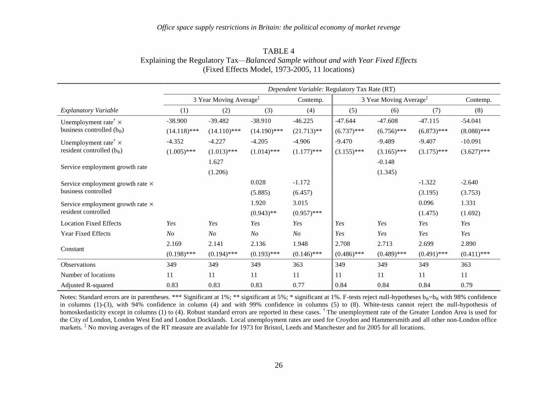
Office space supply restrictions in Britain: the political economy of market revenge
26
TABLE 4
Explaining the Regulatory Tax—Balanced Sample without and with Year Fixed Effects
(Fixed Effects Model, 1973-2005, 11 locations)
Dependent Variable: Regulatory Tax Rate (RT)
3 Year Moving Average‡ Contemp. 3 Year Moving Average
‡ Contemp.
Explanatory Variable (1) (2) (3) (4) (5) (6) (7) (8)
Unemployment rate†
business controlled (bB)
-38.900 -39.482 -38.910 -46.225 -47.644 -47.608 -47.115 -54.041
(14.118)*** (14.110)*** (14.190)*** (21.713)** (6.737)*** (6.756)*** (6.873)*** (8.088)***
Unemployment rate†
resident controlled (bR)
-4.352 -4.227 -4.205 -4.906 -9.470 -9.489 -9.407 -10.091
(1.005)*** (1.013)*** (1.014)*** (1.177)*** (3.155)*** (3.165)*** (3.175)*** (3.627)***
Service employment growth rate 1.627 -0.148
(1.206) (1.345)
Service employment growth rate
business controlled
0.028 -1.172 -1.322 -2.640
(5.885) (6.457) (3.195) (3.753)
Service employment growth rate
resident controlled
1.920 3.015 0.096 1.331
(0.943)** (0.957)*** (1.475) (1.692)
Location Fixed Effects Yes Yes Yes Yes Yes Yes Yes Yes
Year Fixed Effects No No No No Yes Yes Yes Yes
Constant 2.169 2.141 2.136 1.948 2.708 2.713 2.699 2.890
(0.198)*** (0.194)*** (0.193)*** (0.146)*** (0.486)*** (0.489)*** (0.491)*** (0.411)***
Observations 349 349 349 363 349 349 349 363
Number of locations 11 11 11 11 11 11 11 11
Adjusted R-squared 0.83 0.83 0.83 0.77 0.84 0.84 0.84 0.79
Notes: Standard errors are in parentheses. *** Significant at 1%; ** significant at 5%; * significant at 1%. F-tests reject null-hypotheses bB=bR with 98% confidence
in columns (1)-(3), with 94% confidence in column (4) and with 99% confidence in columns (5) to (8). White-tests cannot reject the null-hypothesis of
homoskedasticity except in columns (1) to (4). Robust standard errors are reported in these cases. †
The unemployment rate of the Greater London Area is used for
the City of London, London West End and London Docklands. Local unemployment rates are used for Croydon and Hammersmith and all other non-London office
markets. ‡ No moving averages of the RT measure are available for 1973 for Bristol, Leeds and Manchester and for 2005 for all locations.

Office space supply restrictions in Britain: the political economy of market revenge
27
TABLE 5
Explaining the Regulatory Tax—Balanced Sample with Post 1989 Dummy (Fixed Effects Model)
Dependent Variable: Regulatory Tax Rate (RT)
Entire Period: 1973-2005 Narrow Window Around UBR Introduction: 1985-1994
3 Year Moving Average‡ Contemp. 3 Year Moving Average Contemp.
Explanatory Variable (1) (2) (3) (4) (5) (6) (7) (8)
Unemployment rate†
business controlled (bB)
-38.900 -39.199 -38.910 -46.225 -107.851 -111.489 -127.637 -148.765
(14.139)*** (14.136)*** (14.211)*** (21.744)** (17.821)*** (17.597)*** (18.837)*** (23.676)***
Unemployment rate†
resident controlled (bR)
-3.925 -3.867 -3.856 -4.534 -8.776 -8.758 -8.794 -11.149
(0.812)*** (0.819)*** (0.819)*** (1.066)*** (2.872)*** (3.028)*** (2.805)*** (3.479)***
Service employment
growth rate
0.836 2.851
(1.175) (3.945)
Service empl. growth rate
business contr.
0.028 -1.172 15.507 22.413
(5.894) (6.466) (10.261) (12.666)*
Service empl. growth rate
resident contr.
0.986 2.111 -2.912 -2.877
(0.869) (0.966)** (3.521) (4.039)
Dummy: Post 1989, all
markets except City of L.
0.657 0.648 0.646 0.606 0.481 0.529 0.432 0.400
(0.073)*** (0.073)*** (0.073)*** (0.085)*** (0.118)*** (0.148)*** (0.144)*** (0.172)**
Location Fixed Effects Yes Yes Yes Yes Yes Yes Yes Yes
Year Fixed Effects No No No No No No No No
Constant 1.791 1.782 1.781 1.652 7.185 7.165 7.205 7.438
(0.151)*** (0.151)*** (0.150)*** (0.143)*** (0.606)*** (0.647)*** (0.594)*** (0.675)***
Observations 349 349 349 363 110 110 110 110
Number of locations 11 11 11 11 11 11 11 11
Adjusted R-squared 0.85 0.85 0.85 0.78 0.92 0.92 0.92 0.90
Notes: Robust standard errors are in parentheses. *** Significant at 1%; ** significant at 5%; * significant at 1%. F-tests reject null-hypotheses bB=bR with
98% confidence in columns (1)-(3), with 94% confidence in column (4) and with 99% confidence in columns (5) to (8). White-tests reject the null-
hypothesis of homoskedasticity in all cases. †
The unemployment rate of the Greater London Area is used for the City of London, London West End and
London Docklands. Local unemployment rates are used for Croydon and Hammersmith and all other non-London office markets. We also estimated
specifications using 5 year and 7 year moving averages. The coefficient on the post 1989 dummy variable is virtually unchanged in these cases. ‡ No moving
averages of the RT measure are available for 1973 for Bristol, Leeds and Manchester and for 2005 for all locations.
Office space supply restrictions in Britain: the political economy of market revenge
28
4 report results estimated on data for the whole period with columns 1 to 3 using the three
year moving average of RT and with column 4 using the contemporaneous RT. Columns 5 to
8 show results for exactly comparable models but estimated on just a narrow window of data,
five years either side of 1989. This approach ensures a greater focus on the before-after
transition (by getting rid of the not-so-informative years) and thereby provides a more
demanding test for the hypothesis.16
Comparing the results reported in columns 1 to 3 and 5 to 7 shows that including the office
employment growth rate makes no significant difference to the results for the unemployment
variable. Now with the post-1989 dummy the model continues to perform well but we
observe a significant across the board increase in estimated planning restrictiveness in all
locations compared to the City of London from 1989. The results for the ‗narrow window‘
(columns 5 to 8) confirm this result. The parameter estimate for the post-1989 dummy is
rather smaller but still significant at the 1% level for all except the contemporaneous RT
measure where it is only significant at 5%. The rather smaller value of the dummy parameter
seems intuitively plausible because of the durable nature of real estate. The annual flow of
new office space is small relative to the stock even though, since we are looking at ‗prime‘
office space, the flow will be larger relative to the stock than would be the case of all office
space. Thus one would expect a change which led all locations except the City of London
becoming even more restrictive in their planning policies than previously would have a
cumulative impact on supply, and so prices, over time. The narrow window excludes changes
after 1994 and so is likely to indicate a smaller absolute increase in prices relative to costs (in
other words in the RT) than when the impact of the UBR is estimated over the whole period
for which data are available. Nevertheless, the strong results for the narrow window provide
useful and more direct additional evidence supporting the conclusion that the introduction of
the UBR generated an even stronger incentive for local communities to restrict office
development.
Overall, therefore, these results seem to provide strong support for the interpretations offered
and reinforce our confidence in the RT as a reasonable measure of the impact of planning
restrictiveness on the costs of office space. Although demand and supply may not be fully
identified, the most obvious direct measure of demand – office employment growth – is
hardly significant and, when included in the models, has no impact on the estimated effect of
the unemployment variable, designed to measure local political pressures for the relaxation of
planning restrictiveness. The strongest evidence for the hypotheses, however, is probably
provided by the difference in the estimated impact of the unemployment variable depending
on the form of local political control. The estimates show that business controlled planning
authorities react significantly more strongly to local unemployment than do resident
controlled authorities and that fiscal (dis)incentives for local communities have the expected
impact on permitting development. These results are confirmed whether the contemporaneous
value or a moving average of RT is used as the dependent variable. Since the moving average
measure of RT should minimise the impact of short-term demand shocks this seems to
provide further support for the conclusion that values of RT really do reflect drivers of the
impact of the supply side restrictions.
16
Thanks to an anonymous referee for this suggestion.
Office space supply restrictions in Britain: the political economy of market revenge
29
7 Conclusions
The Regulatory Tax measure of the gross costs of land use regulations for occupiers of
property seems to be a useful one. Although it will not reflect certain forms of regulatory
constraint, such as compliance costs or costs associated with delays and is, therefore, a lower
bound measure, the ease with which it can be estimated is a very substantial advantage. In this
paper, we provide the first estimates for commercial property and show that for office
buildings in British cities the RT is substantially larger than it is in comparable continental
European cities. Despite using different data sources for the international comparison, which
includes the City of London and London West End, we get values for the two London
markets that are very comparable. The conclusion is that supply in the British office market,
like the British residential sector, is highly constrained by regulation and this costs business
occupiers a substantial amount. It is, in effect, a tax on office users. Unless space is perfectly
substitutable in production, therefore, there will be further costs in terms of output and
employment.
We argue that such a level of regulatory restriction – an order of magnitude greater than the
peak observed in the most restricted sector, in the most restricted markets in the US – is to be
expected given the aims of British planning policy, the form of its instruments, the
fragmented geographical scale of decision making (which internalises costs associated with
development but not benefits), and the fiscal disincentive to local communities to allow
commercial development. In this context we would expect differences in regulatory
constraints between those authorities controlled by business interests compared to those
controlled by residents. We are fortunate that the creation of the LDDC and the historical
anomaly of the City of London – controlled by business interests since the middle ages and
exempt from all the major reforms of local government of the modern age – allow us to test
this proposition. We find strong evidence that business control makes a significant difference
to the tightness of regulatory constraints on office building and on the reaction of
restrictiveness to local economic prosperity measured by the unemployment rate. Including a
direct measure of demand for office space and using a moving average to reduce the effect on
RT of demand side shocks makes no difference to the central result, reinforcing our
conclusion that we are observing variation in regulatory constraints – the supply side.
It is also possible to test the hypothesis that regulatory restriction responds to fiscal incentives
and that, in particular, changes in the incentives to allow commercial development resulting
from the introduction of the UBR early in 1990, led to even more restrictive land use
regulation. This, again, is because the City of London was in large measure protected from the
change and continued to be able to levy its own tax on business property. Again, we find
strong evidence that the elimination of any fiscal incentive to permit commercial development
was associated with an increase in the value of the RT in all other British locations relative to
the City of London. This conclusion is confirmed by estimating the models on just a narrow
window of data five years either side of the introduction of the UBR. The UBR, by further
restricting the supply of office space, increased its cost.
Together these findings support our confidence that the RT measure is really capturing – or at
least closely correlated with – the gross costs imposed by land use regulation.
One of the interesting speculations this prompts is about unintended consequences. As
discussed above, the 1980s Conservative government perceived left wing local authorities as
engaged in a concerted effort to frustrate efforts to increase incentives, privatise state

Office space supply restrictions in Britain: the political economy of market revenge
30
industries, sell off social housing and reduce the total tax take. To finance these efforts to
offset the adverse and regressive impact central government actions were perceived as having,
local governments were (perceived to be) increasing their tax revenues from the business rate,
perhaps as part of a punitive anti-business crusade. Central government‘s response was to
introduce the UBR. This removed control of business property taxes from local communities,
turning business property taxes into a national tax. It managed, therefore, not only to
eliminate all tax revenue gains to local communities from commercial real estate development
but to make this fact perfectly transparent. Nevertheless, local governments continued to have
a legal obligation to provide services to local businesses. So it produced a powerful and
transparent fiscal disincentive for local communities to permit any commercial development.
Over time, our results suggest, this has restricted the supply of offices and pushed up the
value of the RT. The increase in business costs this represents may more than offset any costs
that might realistically have been imposed by old-style left wing councils attempting to raise
money from local business rates; especially given the demise of old-style left wing councils
that occurred between 1989 and the present.
TABLE 6
Effect of the Introduction of the Uniform Business Rate
on a Medium Size Office Firm with 1500m2 Space Usage
Increase in Annual Occupation Cost
Based on
3 Year Moving Average RT
(Table 5—Column 3)
Based on
Contemporaneous RT
(Table 5—Column 4)
Office Market in 1989 £ in 2005 £ in 1989 £ in 2005 £
London West End 59823 89555 56119 84010
Croydon 62794 94003 58906 88182
Reading 47251 70736 44326 66356
Bristol 45529 68158 42710 63937
Birmingham 41702 62428 39120 58562
Leeds 41988 62857 39388 58965
Manchester 48639 72813 45627 68304
Newcastle 56926 85219 53401 79942
Edinburgh 36528 54683 34267 51297
Glasgow 38143 57100 35781 53564
Average (all markets) 47932 71755 44964 67312
Indeed, we can quantify this effect because of the fortunate fact that the City of London alone
was given a partial exemption from the UBR. Consider a medium sized firm with about 200
employees. We assume that the firm uses an office building of 1,500 m2. This is about the
smallest office building that can realistically accommodate 200 employees.17 We first ask the
question of how much in UBR such a company would be paying annually, to have a
benchmark against which to compare our results. This calculation is based on an existing
firm/office building in the London Borough of Camden that matches our above brief. The
17
Based on the London Employment Sites Database (Roger Tym & Partners, 2005) the space usage in Inner
London is 19 m2
per office job, suggesting an office building of 3,800 m2 for a medium size firm with 200
employees. Hence, our assumption of 1,500 m2
is a very conservative one, implying that we are underestimating
rather than overestimating the regulation induced increase in annualised occupation cost.

Office space supply restrictions in Britain: the political economy of market revenge
31
building is located at 7/8 Greenland Place, London, NW1 0AP and in 2005 had a rateable
value of £112,250 with the rate multiple set at 42.6p so the firm had a liability for UBR of
£47,819.
Next we explore the (estimated) effect of the UBR on the price of office space via increasing
the RT. Our computations are based on the most conservative and, we believe, most accurate
estimates for the entire balanced sample period (columns 3 and 4 in Table 5): that is a post-
1989 dummy value of either 0.646 or 0.606. Although the estimated impact of the UBR on
our RT measure in our various markets relative to the City of London is assumed to be
uniform (in effect a mean for all markets), the impact on the price of office space in £s in any
given location will vary because the RT is expressed as a quasi-tax relative to MCC, which
varies across markets.
Table 6 illustrates the estimated effect of the UBR on the annual occupation cost of a
hypothetical office building of 1,500 m2 (relative to the City of London) for the two
alternative estimates of the post-1989 dummy. We use market specific yields in 1989 to
transform changes in capital values to changes in annual rent cost or (assuming that other
occupation cost are constant) occupation cost, respectively.
We report the estimated impact both in 1989 terms (when the UBR was introduced) and in
2005 terms, using the Consumer Price all items Index to adjust the values. The latter figure
allows us to compare the regulatory cost imposed by the UBR to the UBR tax itself, that is,
£47, 819 per year for a 1,500 m2
office building in Camden. As is illustrated in Table 6, the
estimated positive impact of the UBR on annual occupation cost is greater across all markets
and both specifications, compared to our benchmark UBR tax estimate.
Thus the implication is that moving to the UBR far from having the intended effect of
reducing business costs had the perverse effect of increasing them. The law of unintended
consequences is powerful indeed.
References
Barker, K. (2003) Review of Housing Supply: Securing our Future Housing Needs: Interim
Report – Analysis, London: HMSO.
Barker, K. (2004) Review of Housing Supply: Final Report - Recommendations, London:
HMSO.
Barker, K. (2006a) Barker Review of Land Use Planning; Interim Report - Analysis, London:
HMSO.
Barker, K. (2006b) Barker Review of Land Use Planning; Final Report - Recommendations,
London: HMSO.
Bertaud, A. and J.K. Brueckner (2005) ‗Analyzing building height restrictions: predicted
impacts and welfare costs‘, Regional Science and Urban Economics, 35 (2), 109-125.
Brown, G.R. and G.A. Matysiak (2000) Real Estate Investment: A Capital Market Approach,
London: FT Prentice Hall.
Brueckner, J.K. (2000) ‗Urban Sprawl: Diagnosis and Remedies‘, International Regional
Science Review, 23, 160-71.
CBRE (2004 & 2005) Global Market Rents, Los Angeles: CB Richard Ellis
Cheshire, P.C. (1973) Regional Unemployment Differences in Great Britain, Regional Papers
II, Cambridge: Cambridge University Press.

Office space supply restrictions in Britain: the political economy of market revenge
32
Cheshire, P.C. (2005) ‗Unpriced Regulatory Risk and the Competition of Rules:
unconsidered implications of land use planning‘, Journal of Property Research, 22,
2/3, 225-244.
Cheshire, P.C. and C.A.L. Hilber (2007) ‗Office Space Supply Restrictions in Britain: The
Political Economy of Market Revenge‘, Munich Personal RePEc Archive (MPRA)
Working Paper, No 5435, April.
Cheshire, P.C. and S. Sheppard (1986) The Economic Consequences of the British Land Use
Planning System: a Pilot Study, Final Report to ESRC.
Cheshire, P.C., and S. Sheppard (2002) 'Welfare Economics of Land Use Regulation', Journal
of Urban Economics, 52, 242-69.
Cheshire, P.C. and S. Sheppard (2005) ‗The Introduction of Price Signals into Land Use
Planning Decision-making: a proposal‘, Urban Studies, 42 (4), 647-663.
City of London (1991) Unitary Development Plan, Department of Planning: Corporation of
London.
Davis Langdon (2005) Spon’s Architects’ and Builders’ Price Book 2005. London: Spon
Press.
Evenson, B. and W.C. Wheaton (2003) ‗Local Variation in Land Use Regulation‘, Brookings-
Wharton Papers 221-260.
Fainstein, S.S. (1994) The City Builders: Property, politics and planning in London and New
York, Blackwell: Oxford.
Fischel, W.A. (2001) The Home Voter Hypothesis: How Home Values Influence Local
Government Taxation, School Finance, and Land-Use Policies, Cambs, Mass:
Harvard University Press.
Gardiner and Theobald (2006) International Construction Cost Survey, London: Gardiner &
Theobald.
Glaeser, E.L. and J. Gyourko (2003) ‗The Impact of Building Restrictions on Housing
Affordability‘, Federal Reserve Bank of New York Economic Policy Review, June.
Glaeser, E.L., J. Gyourko and R.E. Saks (2005) ‗Why is Manhattan so Expensive? Regulation
and the Rise in Housing Prices‘, Journal of Law and Economics, 48 (2), 331-369.
Gyourko, J. and J. Tracey (1991) ‗The Structure of Local Public Finance and the Quality of
Life‘, Journal of Political Economy, 99, 4, 774-806.
Gyourko, J., C. Mayer and T. Sinai (2005) ‗Superstar Cities‘, Working Paper, Wharton
School.
Hendershott, P., C. Lizieri and G. Matysiak (1999) ‗The workings of the London office
market‘, Real Estate Economics 27(2), 365-387.
Hillier Parker (1983) ‗Investors Chronicle – Hillier Parker Rent Index‘, Investors Chronicle,
No. 12, May 1983.
IAURIF (2002) Les Cahiers de L‘IAURIF 135, Paris: IAURIF.
Ihlanfeldt, K. and T. Shaughnessy (2004) ‗An Empirical Investigation of the Effect of Impact
Fees on Housing and Land Markets‘, Regional Science and Urban Economics, 34,
639-661.
Jones Lang LaSalle (2001) Commercial Real Estate Development and the ‘City Offer’,
European Research Report, London JLL.
KingSturge (2003 to 2005) Global Industrial and Office Rents Survey, London: KingSturge.
Mayer, C.J. and C.T. Somerville (2000) ‗Land Use Regulations and New Construction‘,
Regional Science and Urban Economics, 30, 6, 639-662.
Mayo, S. and S. Sheppard (2001) ‗Housing Supply and the Effects of Stochastic Development
Control‘, Journal of Housing Economics, 10, 109-128.
Muellbauer, J. (2005) ‗Property Taxation and the Economy after the Barker Review‘,
Economic Journal, 115 (502), C99-C117.

Office space supply restrictions in Britain: the political economy of market revenge
33
Needham, B. (1992) ‗A Theory of Land Prices when Land is Supplied Publicly: the case of
the Netherlands‘, Urban Studies, 29 (5), 669-686.
Phillips, J. and E. Goodstein (2000) ‗Growth Management and Housing Prices: The Case of
Portland‘, Contemporary Economic Policy, 18, 334-44.
Reading Chronicle (1989), 12 May.
Roger Tym & Partners (2005) Greater London Authority Employment Projections Technical
Paper 2. London Employment Site Database. Technical Notes and Results, London:
Greater London Authority.
Song, Y. and G. Knaap (2003) ‗New urbanism and housing values: a disaggregate
assessment‘, Journal of Urban Economics, 54, 218-238.
Tsolacos, S. (2004) Property Data and Research Themes, mimeo.
Wheaton, W., R. Torto. and P. Evans (1997) ‗The cyclic behaviour of the Greater London
office market‘, Journal of Real Estate Finance and Economics, 15(1), 77-92.

Office space supply restrictions in Britain: the political economy of market revenge
34
Appendix Tables
TABLE A1
Summary Statistics—Data Used to Calculate Regulatory Tax
Variable Obs. Mean Std. Dev. Min. Max.
Unbalanced Sample (1961-2005)
Headline rent per m2 office space (type A, prime),
based on 10 year lease, annualised 480 175.0 157.9 5.60 881.3
Marginal construction cost per m2 (based on prime
office buildings) 480 556.7 357.2 36.9 1472.4
Equivalent yield for office space (type A, prime),
with imputed values prior to 1973† 480 6.69 1.20 4.00 10.56
Vacancy rate (in %), with imputed missing values† 480 9.29 1.60 5.32 15.03
Rent free period in years based on 10 year lease,
annualised average, with imputed missing values† 480 1.55 0.27 0.35 2.40
Imputed capital value per m2 of office space
(adjusted for rent free periods and vacancy rates) 480 2171.5 2291.1 57.9 14554.5
Balanced Sample (1973-2005)
Headline rent per m2 office space (type A, prime),
based on 10 year lease, annualised 363 188.3 159.7 14.0 881.3
Marginal construction cost per m2 (based on prime
office buildings) 363 608.2 307.5 118.5 1472.4
Equivalent yield for office space (type A, prime),
with imputed values prior to 1973† 363 6.48 1.25 4.00 10.56
Vacancy rate (in %), with imputed missing values† 363 9.16 1.61 5.32 15.03
Rent free period in years based on 10 year lease,
annualised average, with imputed missing values† 363 1.56 0.27 0.35 2.40
Imputed capital value per m2 of office space
(adjusted for rent free periods and vacancy rates) 363 2397.0 2416.4 150.3 14554.5
Data Sources: CBRE (prime rent, yield and total occupation cost information), Davis Langdon
(marginal construction cost information), IPD (national void rate index) and ODPM (regional vacancy
rates). †
The methodologies used to impute missing values are described in detail in Cheshire and
Hilber (2007).

Office space supply restrictions in Britain: the political economy of market revenge
35
TABLE A2
Investigated UK Office Markets and Data Availability
Office Market Years with
Available Data
14 Market
Sample
(Unbalanced)
11 Market
Sample
(Balanced)
City of London 1961-2005 Yes Yes
London West End 1961-2005 Yes Yes
London Docklands (Canary Wharf Tower) 1998-2005 Yes No
Croydon (Outer Suburban London) 1965-2005 Yes Yes
London Hammersmith (Inner Suburban London) 1991-2005 Yes No
Maidenhead (South East) 1984-2005 Yes No
Reading (South East) 1965-2005 Yes Yes
Bristol (South West) 1973-2005 Yes Yes
Birmingham (West Midlands) 1965-2005 Yes Yes
Leeds (Yorkshire and Humberside) 1973-2005 Yes Yes
Manchester (North West) 1973-2005 Yes Yes
Newcastle (Upon Tyne) 1965-2005 Yes Yes
Edinburgh (Scotland) 1965-2005 Yes Yes
Glasgow (Scotland) 1965-2005 Yes Yes
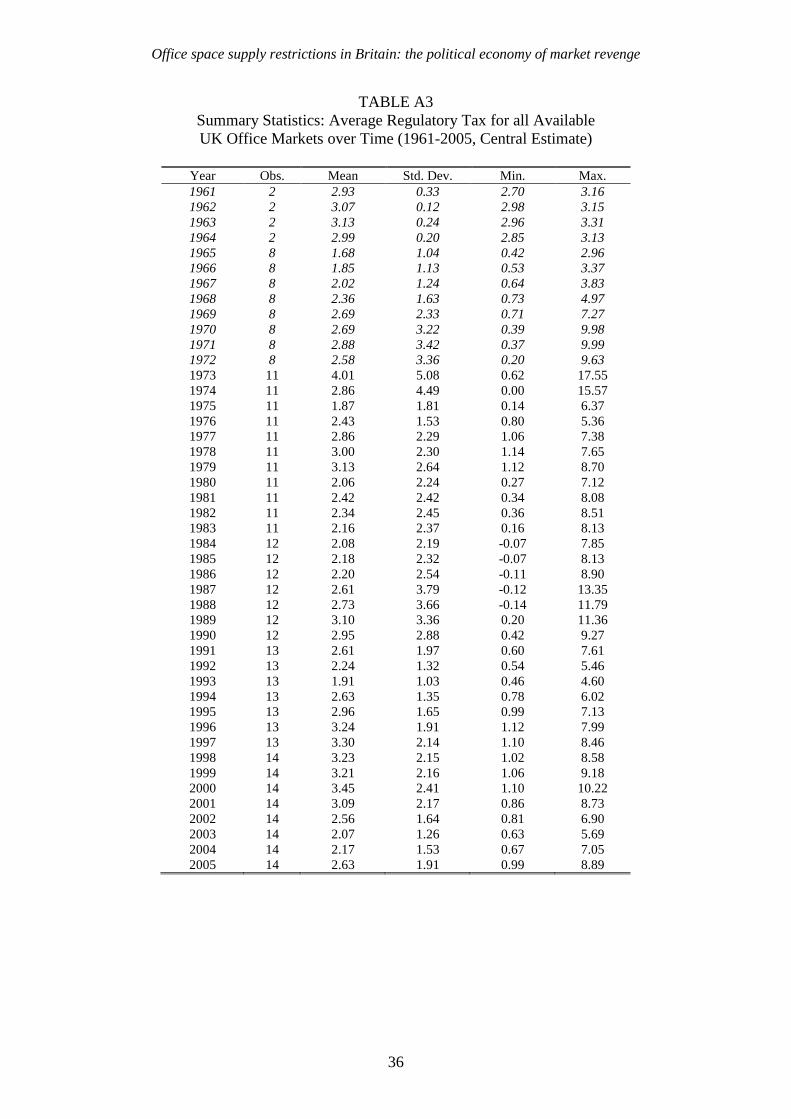
Office space supply restrictions in Britain: the political economy of market revenge
36
TABLE A3
Summary Statistics: Average Regulatory Tax for all Available
UK Office Markets over Time (1961-2005, Central Estimate)
Year Obs. Mean Std. Dev. Min. Max.
1961 2 2.93 0.33 2.70 3.16
1962 2 3.07 0.12 2.98 3.15
1963 2 3.13 0.24 2.96 3.31
1964 2 2.99 0.20 2.85 3.13
1965 8 1.68 1.04 0.42 2.96
1966 8 1.85 1.13 0.53 3.37
1967 8 2.02 1.24 0.64 3.83
1968 8 2.36 1.63 0.73 4.97
1969 8 2.69 2.33 0.71 7.27
1970 8 2.69 3.22 0.39 9.98
1971 8 2.88 3.42 0.37 9.99
1972 8 2.58 3.36 0.20 9.63
1973 11 4.01 5.08 0.62 17.55
1974 11 2.86 4.49 0.00 15.57
1975 11 1.87 1.81 0.14 6.37
1976 11 2.43 1.53 0.80 5.36
1977 11 2.86 2.29 1.06 7.38
1978 11 3.00 2.30 1.14 7.65
1979 11 3.13 2.64 1.12 8.70
1980 11 2.06 2.24 0.27 7.12
1981 11 2.42 2.42 0.34 8.08
1982 11 2.34 2.45 0.36 8.51
1983 11 2.16 2.37 0.16 8.13
1984 12 2.08 2.19 -0.07 7.85
1985 12 2.18 2.32 -0.07 8.13
1986 12 2.20 2.54 -0.11 8.90
1987 12 2.61 3.79 -0.12 13.35
1988 12 2.73 3.66 -0.14 11.79
1989 12 3.10 3.36 0.20 11.36
1990 12 2.95 2.88 0.42 9.27
1991 13 2.61 1.97 0.60 7.61
1992 13 2.24 1.32 0.54 5.46
1993 13 1.91 1.03 0.46 4.60
1994 13 2.63 1.35 0.78 6.02
1995 13 2.96 1.65 0.99 7.13
1996 13 3.24 1.91 1.12 7.99
1997 13 3.30 2.14 1.10 8.46
1998 14 3.23 2.15 1.02 8.58
1999 14 3.21 2.16 1.06 9.18
2000 14 3.45 2.41 1.10 10.22
2001 14 3.09 2.17 0.86 8.73
2002 14 2.56 1.64 0.81 6.90
2003 14 2.07 1.26 0.63 5.69
2004 14 2.17 1.53 0.67 7.05
2005 14 2.63 1.91 0.99 8.89
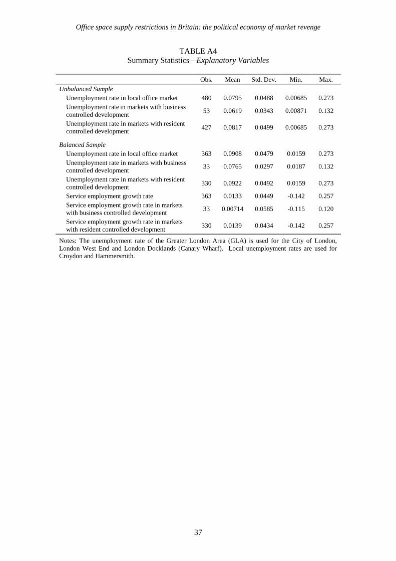
Office space supply restrictions in Britain: the political economy of market revenge
37
TABLE A4
Summary Statistics—Explanatory Variables
Obs. Mean Std. Dev. Min. Max.
Unbalanced Sample
Unemployment rate in local office market 480 0.0795 0.0488 0.00685 0.273
Unemployment rate in markets with business
controlled development 53 0.0619 0.0343 0.00871 0.132
Unemployment rate in markets with resident
controlled development 427 0.0817 0.0499 0.00685 0.273
Balanced Sample
Unemployment rate in local office market 363 0.0908 0.0479 0.0159 0.273
Unemployment rate in markets with business
controlled development 33 0.0765 0.0297 0.0187 0.132
Unemployment rate in markets with resident
controlled development 330 0.0922 0.0492 0.0159 0.273
Service employment growth rate 363 0.0133 0.0449 -0.142 0.257
Service employment growth rate in markets
with business controlled development 33 0.00714 0.0585 -0.115 0.120
Service employment growth rate in markets
with resident controlled development 330 0.0139 0.0434 -0.142 0.257
Notes: The unemployment rate of the Greater London Area (GLA) is used for the City of London,
London West End and London Docklands (Canary Wharf). Local unemployment rates are used for
Croydon and Hammersmith.