User Guide VOLUME 1 – LFS BACKGROUND AND METHODOLOGY 2015

UK Data Archive Study Group Number 33246 - Quarterly Labour Force Survey

Office for National Statistics

1

BACKGROUND AND METHODOLOGY

Contents

SECTION 1 - THE HISTORY OF THE LFS IN THE UK ............................................. 2

SECTION 2 - THE LFS IN NORTHERN IRELAND .................................................... 8

SECTION 3 - SAMPLE DESIGN ................................................................................ 9

SECTION 4 - THE QUESTIONNAIRE ..................................................................... 26

SECTION 5 - FIELDWORK ...................................................................................... 28

SECTION 6 - CODING AND PROCESSING THE DATA ......................................... 42

SECTION 7- NON-SAMPLING ERRORS ................................................................ 45

SECTION 8 - SAMPLING ERRORS AND CONFIDENCE INTERVALS .................. 53

SECTION 9 – NON RESPONSE ............................................................................. 60

SECTION 10 - WEIGHTING THE LFS SAMPLE USING POPULATION ESTIMATES ................................................................................................................................. 62

SECTION 11 - REPORT ON PROXY RESPONSE STUDY BASED ON LFS QUESTIONS ............................................................................................................ 69

SECTION 12 - IMPUTATION IN THE LFS ............................................................... 70

SECTION 13 - CONTINUITY AND DISCONTINUITY ON THE LFS ........................ 75

SECTION 14 – QUALITY ......................................................................................... 85

SECTION 15 - HARMONISATION ........................................................................... 87

SECTION 16 - USES OF THE LFS .......................................................................... 91

SECTION 17 - LFS DISSEMINATION AND PUBLICATIONS .................................. 99

SECTION 18 - LFS DATA FOR SMALL SUB-GROUPS: ANNUAL DATABASES AND AVERAGING OVER SEVERAL QUARTERS ................................................ 103

ANNEX A – PURPOSE LEAFLET ......................................................................... 108

ANNEX B – DERIVATION OF STANDARD ERRORS ON THE LFS ..................... 110

ANNEX C – LABOUR FORCE SURVEY STANDARD ERRORS: JANUARY-MARCH 2015, UNITED KINGDOM ...................................................................................... 112

.

2

SECTION 1 - THE HISTORY OF THE LFS IN THE UK

The Labour Force Survey (LFS) is a survey of households living at private addresses in the UK. Its purpose is to provide information on the UK labour market which can then be used to develop, manage, evaluate and report on labour market policies. The survey is managed by the Social Surveys division of the Office for National Statistics (ONS)1 in Great Britain and by the Central Survey Unit of the Northern Ireland Statistics and Research Agency (NISRA) in Northern Ireland on behalf of the Economic Labour Market Statistics Branch (ELMSB) of the Department of Finance and Personnel. For a more detailed description of the LFS and how it has developed, see:

the August 2006 edition of Labour Market Trends “Reflections on fifteen years of change in using the LFS: How the UK’s labour market statistics were transformed by using the LFS”, by Barry Werner (http://www.ons.gov.uk/ons/rel/lms/labour-market-trends--discontinued-/index.html).

the November 2013 release on “Forty years of change: UK’s biggest survey marks its 40th birthday” http://www.ons.gov.uk/ons/rel/mro/news-release/forty-years-of-change--uk-s-biggest-survey-marks-its-40th-birthday/uk-s-biggest-survey-marks-its-40th-birthday.html which has also been summarised in an infographic http://www.ons.gov.uk/ons/infographics/40-years-of-the-labour-force-survey/index.html

1.1 LFS 1973-1983 The first LFS in the UK was conducted in 1973, under a Regulation derived from the Treaty of Rome. The Statistical Office of the European Union (Eurostat) co-ordinates information from labour force surveys in the member states in order to assist the EC in matters such as the allocation of the European Social Fund. The ONS is responsible for delivering UK data to Eurostat. The survey was carried out every two years from 1973 to 1983 in the spring quarter (March-May) and was used increasingly by UK Government departments to obtain information which could assist in the framing and monitoring of social and economic policy. By 1983 it was being used by the Employment Department to obtain measures of unemployment on a different basis from the monthly claimant count and to obtain information which was not available from other sources or was only available for census years, for example, estimates of the number of people who were self-employed. Published LFS estimates for 1973-1983 refer to the spring quarter and are available on a UK basis.

1 Until 5 July 1995, the LFS was the responsibility of the Employment Department (ED). On that date

ED was abolished and responsibility for the survey passed to the Central Statistical Office (CSO). On 1 April 1996, the CSO merged with the Office for Population Censuses and Survey (OPCS) to form the ONS which now has responsibility for the LFS.

3

1.2 ANNUAL LFS 1984-1991 Between 1984 and 1991 the survey was carried out annually and consisted of two elements:-

(i) A quarterly survey of approximately 15,000 private households, conducted in

Great Britain throughout the year;

(ii) A "boost" survey in the spring quarter between March and May, of over 44,000 private households in Great Britain and 5,200 households in Northern Ireland.

Published estimates for 1984-1991 are available for the UK and are based on the combined data from the “boost” surveys and quarterly surveys in the spring quarters (Mar-May). The quarterly component of the 1984 to 1991 surveys were not published because the small sample sizes meant that the results were not robust. However, the quarterly survey proved to be invaluable in developmental terms, and in making early assessments of seasonality. A fuller description of the survey methodology used in this period is available in the annual results published by ONS (previously by OPCS) - see section 17 for details of these publications. 1.3 QUARTERLY LFS FROM SPRING 1992 In 1992 the sample in GB was increased to cover 60,000 households every quarter enabling quarterly publication of LFS estimates. Whilst it built on the annual survey, there were a number of differences which can be summarised as follows:

(i) panel design – from 1992 the GB survey was based on a panel design where a fifth of the sample each quarter is replaced and individuals stay in the sample for 5 consecutive waves or quarters. A shorter fieldwork period was also introduced which together with the panel nature of the survey led to slightly lower response rates.

(ii) sample design - the major difference was the introduction of an

unclustered sample of addresses for the whole of Great Britain (the sample for Northern Ireland is similarly unclustered). This improved the precision of estimates particularly when making regional analyses. In the case of Scotland a very small bias arises from partial coverage of the population north of the Caledonian Canal. This area contains about five percent of the total population of Scotland.

(iii) additions to the sample - the inclusion of people resident in two

categories of non-private accommodation, namely those in NHS accommodation and students in halls of residence. The students are included through the parental home.

In the winter of 1994/95 a quarterly Labour Force Survey was introduced to Northern Ireland. Each quarter's sample consists of approximately 3,000 household responses spread over five waves - 600 in each wave. A rotational pattern was also

4

adopted, identical to that being operated in the GB LFS. Quarterly UK LFS estimates are available from winter 1994/95. 1.4 LFS QUARTERS The quarterly LFS launched in 1992 in GB and in 1994 in NI operated on a seasonal quarter basis: March-May (Spring), June-August (Summer), September-November (Autumn) and December-February (Winter). The reasons for this were: -

(i) Many activities associated with the labour market occur seasonally and follow the pattern of the school year. This was more the case when the LFS first started at which point more young people left school at Easter than in the summer;

(ii) Easter can cause difficulty as it varies in timing between March and

April – so ensuring that Easter is always covered by the same quarterly survey period avoids this problem.

The first results from the quarterly GB LFS, relating to spring 1992, were published in the LFS Quarterly Bulletin (LFS QB) in September 1992 - that is, about 3½ months after the end of the survey period. From this date, the QB was the main source of LFS data. More timely results were presented in each quarter's ONS 'Labour Force Survey First Release' which provided key results about six weeks after the end of the survey period. Both the QB and the First Release presented GB estimates as Northern Ireland estimates were only available for the Spring quarters until Winter 94/95. 1.5 CALENDAR QUARTERS In May 2006 the LFS moved to calendar quarters (CQ’s). This means the micro data will no longer be available on a seasonal basis (spring – winter). The main reason ONS is moving to CQ’s for the LFS is that it is an EU requirement under regulation2. Eurostat – the body responsible for the EU LFS – has a target structure for the survey with all Member States providing data on a CQ basis which will promote comparability across countries. In addition to conforming to the EU regulation, the switch from seasonal to calendar quarters will also enhance the comparability of the LFS with other quarterly surveys which are mostly conducted on a CQ basis. This is particularly relevant with respect to National Accounts. The following table shows the resultant changes to the quarterly release of micro data.

Seasonal Quarters Calendar Quarters (CQ’s) – from May 2006

Winter (December to February) Q1 = January to March (JM)

Spring (March to May) Q2 = April to June (AJ)

Summer (June to August) Q3 = July to September (JS)

Autumn (September to November) Q4 = October to December (OD)

2 Council Regulation (EC) No 577/98 and associated revisions.

5

This means the spring (March-May) questionnaire will move to the April-June questionnaire (Q2) and the June-August questionnaire will move to the July-September (Q3) and so on. Changes were also made to the interview weeks to align them to CQ’s. A note has been published in the June 2006 (Labour Market Trends http://webarchive.nationalarchives.gov.uk/20160105160709/http://www.ons.gov.uk/ons/rel/lms/labour-market-trends--discontinued-/index.html) which looks at the impact of the move to CQ’s. There is also a CQ version of the Historical Quarterly Supplement (HQS) that was published on 17 May 2006 to coincide with the move. This will have historical data back to 1997 for certain quarters (mostly Q2 and Q4), so that users can look at trends based on CQ’s. A partial series of micro data based on CQs has also been created covering the following periods: Q2 regional datasets 1997, 1999, 2001, and every quarter from then onwards. A full back-series of micro data on a CQ basis has been produced. 1.6 EARNINGS FROM EMPLOYMENT QUESTIONS FROM WINTER 1992/93 Whilst questions in the LFS are continually being added, removed or modified, the major change to the early quarterly survey was the introduction of a section of earnings questions in GB from winter 1992/93 onwards. These questions were only asked of respondents receiving their fifth and final interviews, because of concerns that the questions might have an adverse impact on overall response rates. Results from these earnings questions were first published in the summer 1994 QB (in December 1994), and in the December 1994 Employment Gazette. Earnings questions have been asked in the Northern Ireland LFS since the survey went quarterly in Winter 1994/5 but results were not weighted up until early 1998. LFS earnings data on a UK basis are available for each quarter from Winter 1994/5. 1.7 EARNINGS QUESTIONS FROM SPRING 1997 The LFS is an important source of earnings data, particularly for part-time workers. However, because earnings questions were initially only asked in wave 5 interviews, sample sizes were quite small and associated sampling errors tended to be relatively high. Work was done to test whether asking earnings questions in the first wave would lead to higher non-response in later waves, but no evidence was found to support this. So from Spring 1997 earnings questions were asked in both waves 1 and 5 in GB and NI, doubling the sample size and reducing sampling errors by about 30%. For more detail see ‘Expanding the coverage of the earnings data in the LFS’ in April 1998’s Labour Market Trends. 1.8 MONTHLY PUBLICATION FROM WINTER 1997/8 A major public consultation on labour market statistics was conducted by ONS during 1997, resulting in a new integrated Labour Market Statistical Bulletin (LM SB), (previously called Labour Market Statistics First Release) first published in April 1998 (see February 1998 Labour Market Trends article ‘Improved Labour Market

6

Statistics’). The LM SB, which is published monthly, gives prominence to the ILO measure of unemployment, as measured by the LFS over the administrative claimant count measure and draws together statistics from a range of sources to provide a more coherent picture of the labour market. The claimant count is not an alternative measure of unemployment. LFS results in the LM SB are published on a UK basis, 6 weeks after the end of the survey period, and relate to the average of the latest three-month period. For the latest release see: http://www.ons.gov.uk/ons/rel/lms/labour-market-statistics/index.html Since April 1998, the Economic Labour Market Statistics Branch (ELMSB) of the Department of Finance and Personnel have published a Northern Ireland Labour Market Statistics Release to the same timetable as publication of the Labour Market Statistics First Release 1.9 Enhancements of the LFS in England, Wales and Scotland. Since March 2000 extra respondents have been included as an annual enhancement to the sample size of the LFS. In March 2000 this was just for England, (and was known as the English Local LFS boost (ELLFS)) though was expanded to Wales (WLFS boost) in 2001/02 and Scotland (SLFS) in 2003/04. These boost cases are interviewed annually for four years. More information on this can be found in the Volume 6 (APS) User Guide : https://www.ons.gov.uk/employmentandlabourmarket/peopleinwork/employmentandemployeetypes/methodologies/labourforcesurveyuserguidance#labour-force-survey-lfs-user-guides The aim of the enhancements is to improve labour market information at a local level, as smaller sub-groups of the population can be looked at due to a larger sample. When the results from the enhancements to the LFS in England, Wales and Scotland are combined, it is known as the Annual Local Area Labour Force Survey (ALAFS). More information on the methodology behind the ELLFS can be found in the May 2000 and January 2002 issues of the Labour Market Trends 1.10 The Annual Population Survey In 2004, a further improvement, the Annual Population Survey (APS), was introduced. The APS included all the data of the ALALFS, but also included a further sample boost in more urban areas of England – known as the APS(B) - aimed at achieving a minimum number of economically active respondents, in the sample, in each Local Authority District in England. The respondents included in the boost were not asked all the questions in the main LFS, see user guide Volume 6 for more information.

7

The first APS covered the calendar year 2004 rather than the ALALFS period of March to February. The ALALFS data was only published once a year, whereas the APS data is published quarterly, with each publication including a year's data, In 2006, funding for the APS(B) was withdrawn, and so the structure of the Annual Population Survey reverted to the same as the ALALFS (that is, waves 1 and 5 of the quarterly LFS plus the ELLFS, WLFS, and SLFS). However, the name ‘Annual Population Survey’ has been retained, and the data continues to be published four times a year. Currently a quarterly main LFS dataset contains around 100,000 individuals, and an APS dataset contains around 320,000 individuals.

8

SECTION 2 - THE LFS IN NORTHERN IRELAND

The Northern Ireland Labour Force Survey is the responsibility of Economic Labour Market Statistics Branch (ELMSB) of the Department of Finance and Personnel and fieldwork is carried out by the Central Survey Unit of the of the Northern Ireland Statistics and Research Agency (NISRA). From 1973 - 1983, as in GB, the survey in Northern Ireland was conducted in alternate spring quarters. From 1984 - 1994 it was carried out annually. This annual survey consisted of 5,200 addresses drawn at random from the Rating and Valuation List - approximately 1% of private addresses in Northern Ireland. Over this period interviewing was conducted only in the spring, with no quarterly element. UK LFS estimates are available for Spring quarters from 1973-1994. In the winter of 1994/95 a quarterly Labour Force Survey was introduced to Northern Ireland. Each quarter's sample consists of approximately 3,000 household responses spread over five 'waves' - 600 in each wave. A rotational pattern was also adopted, identical to that being operated in the GB LFS. Respondents at 'wave' 1 are interviewed face-to-face with subsequent interviews at 'waves' 2-5 taking place, where possible, by telephone. Computer assisted interviewing has been used in the Northern Ireland Labour Force Survey since 1992. Quarterly UK LFS estimates are available from winter 1994/95. Income questions have been asked in the Northern Ireland LFS since the survey went quarterly in Winter 1994/5 but results were not weighted up until early 1998. LFS income data on a UK basis is now available for each quarter from Winter 1994/5. From Spring 1997, the income questions in both the GB and NI LFS have been asked of respondents in waves 1 and 5, producing a larger sample size then when previously asked only of wave 1 respondents. Since April 1998, the Economic Labour Market Statistics Branch (ELMSB) have published a Northern Ireland Labour Market Statistics Release to the same timetable as publication of the Labour Market Statistics Bulletin.

9

SECTION 3 - SAMPLE DESIGN The Labour Force Survey (LFS) is the largest regular social survey in the United Kingdom. The Office for National Statistics (ONS) conducts the survey in Great Britain, and its implementation in Great Britain is the responsibility of ONS’ Social Survey Division, which works in close co-operation with ONS’ Methodology Directorate. The Central Survey Unit of the Northern Ireland Statistics and Research Agency (NISRA) conducts the survey in Northern Ireland. The designs of both the Great Britain and Northern Ireland surveys are similar. Though a quarterly survey, the design of the LFS and fieldwork procedures enable estimates of levels, such as the number of people in employment, to be produced for rolling three-monthly periods. Such estimates are published in the monthly Labour Market Statistics statistical bulletin. This section of the User Guide examines the sampling procedures used in the LFS, the sample design has implications on the weighting used in the survey (see Section 10) and calculation of standard errors (Section 8). It also has close links with Fieldwork (Section 5), Non-response (Section 9) and Imputation (Section 12).The National Statistics Quality Review (NSQR) also contains some additional information: http://webarchive.nationalarchives.gov.uk/20160105160709/http://www.ons.gov.uk/ons/guide-method/method-quality/quality/quality-reviews/list-of-current-national-statistics-quality-reviews/nsqr-series--2--report-no--1/index.html 3.1 TARGET POPULATION 3.1.1 Private Households The target population of the LFS is based on the resident population in the United Kingdom. Specifically, the LFS aims to include all people resident in private households, resident in National Health Service accommodation, and young people living away from the parental home in a student hall of residence or similar institution during term time. (This latter group is included in the LFS sample specifically to improve the coverage of young people.) The sample currently consists of around 38,000 responding (or imputed) households in Great Britain every quarter, representing about 0.15% the GB population. Data from approximately 1,500 households in Northern Ireland are added to this, representing about 0.21% of the NI population, allowing analysis of data relating to United Kingdom. For most people, the meaning of residence at an address is unambiguous, and people with more than one address are counted as resident at the sampled address if they regard that as their main residence. The following are also counted as being resident at an address:

1. people who normally live there, but are on holiday, away on business, or in hospital, unless they have been living away from the address for six months or more;

2. children aged 16 and under, even if they are at boarding or other schools;

10

3. students aged 16 and over are counted as resident at their normal term-time address even if it is vacation time and they may be away from it.3

3.1.2 Communal Establishments and Non-Private Households The LFS relates mainly to the population of the UK resident in private households, with the exception of NHS accommodation and student halls of residence. Therefore, this section of the User Guide has been included to assist users who wish to form a more complete picture of the UK population. The 2001 and 2011 Population Census definitions state that communal establishments (CEs) provide managed residential accommodation4. Examples of CEs include residential care homes and university halls of residence. LFS outputs relate almost exclusively to the population living in private households, and, with a couple of notable exceptions, exclude most of the population living in CEs. Of social surveys in the UK, the LFS is not alone in excluding CEs from its sampling frame; the Living Costs and Food Survey (LCF) and the Family Resources Survey do not sample from CEs either. Some departments (for example the Department of Health) do, however, occasionally conduct samples of sub-sets of the CE population. At present, the decennial Population Census is the most reliable source of CE population data. Over recent years ONS has investigated options for surveying CEs on a more regular basis5, but the main statistical obstacle remains the lack of a suitable, comprehensive and readily available sampling frame for all CEs. Comparisons between LFS and Census estimates of the residents of communal establishments suggest that residents of CEs tend to differ from the rest of the population in terms of their demographic characteristics. The main differences are:

there are proportionately more women in CEs

the population is generally older in CEs, especially for women

the economic activity rate is considerably lower amongst CE residents. Table 3.1 provides estimates of the population resident in CEs in Great Britain from the 2011 Census.

3 For the LFS: adult children living in halls of residence will be included at the parental address. For

other ONS surveys a different definition exists The standard ONS instruction for defining a household states ‘Adult children, that is, those aged 16 and over who live away from home should not be included at their parental address’. 4 See Population Definitions for 2001 Census (Census Advisory & Working Groups), Advisory Group

Paper (99)04; and Final Population Definitions for the 2011 Census: http://www.ons.gov.uk/ons/rel/census/2011-census/population-and-household-estimates-for-the-united-kingdom/stb-2011-census--population-estimates-for-the-united-kingdom.html 5 Communal Establishment Survey, Findings of the Pilot Stage: Summary Report, ONS (2009):

11

Table 3.1: Communal Establishments and their resident populations in Great Britain, as recorded by the 2011 Population estimates.

Number of residents

Medical and care establishments 463,055

NHS 14,601

General Hospital 2,317

Mental health hospital/unit

(including secure units) 9,043

Other hospital 3,241

Local Authority 23,551

Children's home (including secure

units) 1,678

Care home with nursing 2,014

Care home without nursing 18,612

Other home 1,247

Registered Social Landlord /

Housing Association 7,150

Home or Hostel 4,939

Sheltered housing only 2,211

Other 417,753

Care home with nursing 174,025

Care home without nursing 223,462

Children's home (including secure

units) 3,023

Mental health hospital/unit

(including secure units) 5,490

Other hospital 2,665

Other establishment 9,088

Other establishments 640,761

Defence 46,661

Prison service 59,243

Approved premises

(probation/bail hostel)1 1,161

Detention centres and other

detention 12,188

Education 425,351

Hotel, guest house, B&B, youth

hostel 30,402

Hostel or temporary shelter for

the homeless 23,601

Holiday accommodation (for

example holiday parks) 3,682

Other travel or temporary

accommodation 4,192

Religious 6,237

Staff/worker accommodation only 4,897

Other 23,146

Total residents 1,103,816 1 Not applicable in Scotland

Type of communal establishment

12

Communal Establishments: The International Dimension Although the LFS is carried out under European Regulation, Eurostat acknowledges the difficulties associated with sampling communal establishments; it recognises that “for technical and methodological reasons it is not possible ... to include the population living in collective households,” (Eurostat, EU LFS Methods and Definitions 2001, p10). The requirement is therefore to provide only results for private households only in the LFS, and many of the Labour Force Surveys run by other European Union member states also exclude communal establishments. In the Labour Force Surveys of Australia, Canada and the USA, the sampling frames for the Labour Force Survey are designed to represent the civilian non-institutional population and therefore exclude:

full-time members of armed forces,

residents of institutions such as prisons and mental hospitals, and

patients in hospitals or nursing homes who have been there at least 6 months. In Australia some effort is made to include non-household residents using a list sample of non-private dwellings such as hotels and motels. The US equivalent of the LFS (the ‘Current Population Survey’) also attempts to include such people; the stratified sampling frame includes a ‘group quarter’ stratum containing those housing units where residents share common facilities or receive formal care.

3.2 SAMPLE DESIGN AND WAVE PATTERNS OF THE LFS The LFS uses a rotational sampling design, whereby a household, once initially selected for interview, is retained in the sample for a total of five consecutive quarters. The interviews are scheduled to take place exactly 13 weeks apart, so that the fifth interview takes place one year on from the first. We define Wave 1 to be the first quarter an address is selected, Wave 2 to be its second quarter in the selection, and so on. Therefore, Wave 5 is the last time that household will be interviewed for the main LFS. We stress here that it is the address that is selected for five quarters and not necessarily the particular people who live there. Therefore, it is possible to ‘find’ people new in the sample in Waves other than Wave 1, though the majority of people are first found in Wave 1. It is also possible for people to drop out of the sample before Wave 5 if they move to a different address. The main reasons for use of a rotating sample design are:

the precision of estimates of change over time is improved where there is overlap in the sample. Thus, better estimates of quarter-on-quarter and quarter on same-quarter-a-year-ago can be produced with this wave pattern;

longitudinal data sets can be produced, which may be used for analysis of gross change (i.e. change in individuals’ circumstances)

The same number of Wave 1 (new) addresses are selected each quarter. So, in any given quarter, about one-fifth of the addresses in the entire sample are in Wave 1, one-fifth in Wave 2, and so on. Thus, between any two consecutive quarters, about 80% of the selected addresses are in common. Figure 3.1 shows this pattern.

13

Figure 3.1: Wave patterns in the LFS.

LF

S

Co

ho

rt 1

LF

S

Co

ho

rt 2

LF

S

Co

ho

rt 3

LF

S

Co

ho

rt 4

LF

S

Co

ho

rt 5

LF

S

Co

ho

rt 6

LF

S

Co

ho

rt 7

LF

S

Co

ho

rt 8

LF

S

Co

ho

rt 9

LF

S

Co

ho

rt 1

0

LF

S

Co

ho

rt 1

1

LF

S

Co

ho

rt 1

2

JM14 W5 W4 W3 W2 W1

AJ14 W5 W4 W3 W2 W1

JS14 W5 W4 W3 W2 W1

OD14 W5 W4 W3 W2 W1

JM15 W5 W4 W3 W2 W1

AJ15 W5 W4 W3 W2 W1

JS15 W5 W4 W3 W2 W1

OD15 W5 W4 W3 W2 W1 The labelling of Cohorts in the diagram is arbitrary, and the same colour represent the same cohort of households. Using JM14 as example, we see that Cohort 5 (the dark green boxes), are having their Wave 1 interviews. In the same quarter, Cohort 4 will be having their Wave 2 interviews, Cohort 3 their Wave 3 interviews, Cohort 2 their Wave 4 interviews, and Cohort 1 their Wave 5 / final interviews. Moving on one quarter to AJ14, and Cohort 5 are now having their Wave 2 interviews, Cohort 4 Wave 3 and so on. Cohort 1 is not interviewed in this quarter, and in it place, Cohort 6 has been selected for the first time and is on Wave 1 interviews. Since each wave contains the same number of selected addresses, there is an 80% overlap between any two consecutive quarters. For example, between JM14 and AJ14, Cohort 2, 3, 4 and 5 are in common, Cohort 1 has been dropped and Cohort 6 is newly selected.

The LFS Waves in Great Britain were first created in the build-up period of the quarterly survey (autumn 1991 and winter 1991/92). Further details of this are reported in the 2009 (and earlier) editions of the LFS User Guide Volume 1. The same pattern of waves is used in both Great Britain and Northern Ireland, but for the latter an additional sample, known as a booster, exists. For the booster, 260 new Northern Ireland addresses (in addition to the usual new sample of 650) are added in Quarter 2 each year, and these are spread evenly amongst the five waves. Thus a booster address assigned to Wave 1 will have four subsequent interviews, whereas one assigned to Wave 5 will have no subsequent interviews. 3.3 SAMPLING FRAMES AND SAMPLE SELECTION Four different sampling frames are used in the UK Labour Force Survey. Great Britain is split into two areas: south of the Caledonian Canal, comprising all of England, Wales and most of Scotland; and north of the Caledonian Canal in Scotland. Northern Ireland has its own sampling frame. A separate list of NHS accommodation in Great Britain is maintained. The Wave 1 sample is selected by first ordering the sampling frames geographically, and then drawing the selection systematically (that is, with a fixed interval). The

14

subsequent waves are not drawn from the frames; the Wave 1 selections are simply retained and become Wave 2 interviews in the next quarter, and so on. For the most part, the LFS may be regarded as a single-stage sample of households each quarter, though changes made in 2010 (see Section 3.5) mean this is no longer strictly the case. The geographical ordering of the frame implicitly stratifies the sample, ensuring a geographic spread of addresses. Since all adults within a household are sampled, the person-level survey may be regarded (mainly) as a one-stage cluster sample of people, with the clusters (or primary sampling units) being the households. We now look in more detail at each of the frames used, and how the selection of the Wave 1 sample is made. The information given refers to the number of addresses that are selected. Of course, not all of the addresses selected lead to a response, and we examine the number of responses in Section 3.7. 3.3.1 Sampling Households South of the Caledonian Canal in Great Britain The sampling frame used for private households in Great Britain south of the Caledonian Canal is the Postcode Address File. The PAF is a computerised list, owned by Royal Mail, of all the addresses to which mail is delivered. The PAF is updated by ONS every six months. The actual frame used for the LFS, and most other ONS social surveys, is the ‘small users file’, a sub-file of the complete PAF. 'Small users' are defined as delivery points which receive relatively few items of mail per day. This automatically excludes from the frame many businesses and other non-household institutions. However, the small users file still contains some non-private and non-residential (therefore ineligible) addresses, which cannot be identified prior to the interviewer making contact. Interviewers have instructions to exclude such institutions and classify them as ineligible. The number of addresses selected from the PAF for Wave 1 each quarter is currently 16,640 – a number that has remained constant for many years now. The selection process currently employed is as follows:

The complete frame of delivery points is first ordered by Postcode, and within that by address.

The sampling interval, k, (required for systematic sampling) is then calculated by dividing the total number of addresses (that is delivery points in England and Wales, and the multi-occupancy size marker in Scotland) by 16,640. This currently gives a 1-in-1586 Wave 1 quarterly sample size.

A random start is chosen from {1, 2, …, k}, and that address and every kth one after it are marked. This selection creates what is called the pre-sample.

To ensure no household is over-burdened, a Used Address File is maintained, such that an address used for sampling in any ONS social survey will not be sampled again for some two years or so after the final interview. To enable this, while also reducing any potential bias in small, local areas, the actual sample is then selected as follows:

15

The number of marked addresses in each Postcode Sector (e.g. AB12 3..) is counted.

A new systematic sample is then drawn separately for each Postcode sector from addresses not on the Used Address File. The sampling interval used in each Postcode sector is calculated so as to select the number of addresses required for that sector, as counted in the pre-sample.

All selected addresses (across all the five waves) are then allotted to pre-determined Interviewer Areas, and within those into weekly stints, 13 of which make up the quarter’s interviews. More detail is given in Section 3.4.2. 3.3.2 Sampling Households North of the Caledonian Canal in Scotland A different approach is taken for sampling north of the Caledonian Canal in Scotland. The canal runs from Corpach near Fort William on the west coast, through the lochs of Great Glen to Inverness on the east coast. The area to the north is sparsely populated, which means that interviewing a single-stage sample of addresses from the PAF face-to-face would be prohibitively expensive. An option of using a two-stage (clustered) sample design was considered, but the ultimate decision was taken to use a one-stage sample drawn from the telephone directory, along with telephone interviewing. The sampling interval used on the main LFS sample south of the Caledonian Canal is used to determine the number of addresses to sample size north of the canal. Currently 80 addresses are selected for Wave 1 each quarter. Addresses are then selected systematically from the appropriate telephone directories, with the first one chosen with a random start, and following on in the directory from where the previous quarter’s sample finished. Additional checks are made to ensure that the selected address is actually located north of the Caledonian Canal, and is not on the Used Address File. The main disadvantage of sampling from telephone directories is the potential bias resulting from non-coverage of people not listed in the directory (e.g. those with no phone at all, a mobile phone only, ex-directory, or in a new-build property that is not yet listed). However, the alternative of a two-stage sample of addresses interviewed face-to-face would still have led to large sampling errors and would also still incur high travel costs in the area. 3.2.3 Sampling Households in Northern Ireland The sampling frame used in the Northern Ireland LFS is POINTER, which is the government's central register of domestic properties. It excludes commercial units. Land & Property Services (LPS) owns and maintains the register, and it is based on addresses held by the Ordnance Survey of Northern Ireland. It is updated two-to-three times a year, by LPS, the Northern Ireland District Councils, the Rates Collection Agency and other sources. A similar selection procedure is used to that on the PAF, except the selection is made in one pass. Addresses that have been used recently for surveys are known as being ‘flagged’ in Northern Ireland, and these cannot be selected for the current

16

period survey. As with the PAF, the frame is sorted geographically, ensuring a regional spread of sample addresses. The frame is sorted first by District Council, then by Ward and then by address. The quarter’s fieldwork is spread over three months, and a new sample is drawn every month. Total monthly sizes for the three months in a calendar quarter are 200, 250 and 200, giving a quarterly total of 650 Wave 1 (new) addresses. This currently represents a 1-in-1185 Wave 1 sample of all domestic properties in Northern Ireland. Additionally, 260 additional (‘booster’) new addresses are added to the sample in Quarter 2 of each year; these are spread equally across the five waves. Allocation to interviewers is on a dynamic basis, and takes into account total interviewing requirements and interviewer-availability. 3.3.4 Sampling NHS Accommodation The sampling frame for NHS accommodation was specially developed for the Labour Force Survey. All district health authorities and NHS trusts were asked to supply a complete list of their accommodation (this accommodation mainly comprises what was once known as 'Nurses Homes', but the coverage is more extensive than that name implies)6. The proportion of addresses to sample is calculated by comparing the list with the PAF. Currently nine units of NHS accommodation in Great Britain are selected for Wave 1 interviews each quarter. 3.4 FURTHER NOTES ON SAMPLING 3.4.1 Multiple-occupancy addresses Different sampling procedures exist at multiple-occupancy addresses, that is at those addresses at which more than one household resides or is likely to reside. Some of the more common examples include apartment blocks with just one front door, or a house which has been converted into flats. In Scotland, the Multiple-Occupancy marker on the PAF serves as a reliable guide to identifying the existence of multiple households behind the one front door. The marker is that used by the Post Office. Within England, Wales, and sometimes still in Scotland and Northern Ireland, it is only when an interviewer first makes contact at the property that its multiple-occupancy structure becomes clear. In these cases, once the number of households present is established, just one of them is selected, at random, for interview. Section 3.5 gives more detail. A slightly different scenario is that of the divided address. Again, typically, these are often one building that has been split into separate addresses. However, each address is listed separately on the PAF, but a marker is provided on all that belong to the one ‘divided address’. In these cases, if it is the address with the highest

6 Information was received from 417 out of the 455 authorities, trusts and teaching hospitals and the

frame is not therefore complete. If the coverage of the frame is proportional to the coverage of authorities etc., then the frame contains 92 per cent of all NHS accommodation.

17

address key (PAF unique identifier) within the building that is selected, the interviewer is asked to check there are no other addresses in existence in the building with the same postcode, that are not listed on the PAF. If there are, again it is just one that is selected for interview. This procedure attempts to ensure that all addresses in existence have a chance of selection. 3.4.2 Interviewer area allocations We give some more details here of the way in which interviews are allocated to interviewers south of the Caledonian Canal. Further detail can be found in Section 5 of this volume of the LFS User Guide.

The selected sample falls within 208 Interviewer Areas. These interviewer areas are split into "quotas", generally 2 in each interviewer area.

For LFS fieldwork each quota is then divided into 13 stints, each stint containing roughly the same number of Delivery points (or MOs for Scotland). The Interviewer Areas are comprised of mainly two quotas, though there are some with one or three quotas (there are 318 quotas in England, 51 in Wales and 43 in Scotland).

The 13 stints are randomly allocated to the 13 weeks of a quarter, and these are labelled 01 to 13. The Stint plus the week number form the quota number the same quota is covered by an LFS interviewer in the same week each quarter. Most interviewers cover two quotas . The design of the stinting is such that quotas are 'paired' so that an interviewer can be given 2 quotas of work they will be neighbouring. For example stint 901 and 902 are paired, so quotas 90101 and 90201 will be next to each other and any addresses which fall in those quotas will be interviewed in week one of the quarter.

All postcodes are plotted on the boundary maps for the quotas, and the quota they fall in is held on the Sampling system. The systematic random sample of addresses selected for the quarter throughout the country is matched to it's quota on postcode to provide a list of addresses to be interviewed each week.

A “Leap Week” is introduced periodically to re-align ‘LFS quarters’ (of 13 weeks) with calendar quarters, which gradually move out of alignment, as four quarters of 13 weeks give only 364 days, just short of a calendar year. The most recent LFS Leap Week was in October 2015 and was included to bring the LFS survey month into line with Eurostat regulations; the previous ones were in 2010 and in 2004. The Leap Week sees no LFS interviews take place (other than those left over from the previous week), and it is contained in neither the reference quarter before nor after.

3.4.3 Data collection modes Most households are interviewed face-to-face at their first inclusion7 in the survey and by telephone, if possible, at quarterly interviews thereafter. Respondents are encouraged to provide a telephone number and agree to interview in subsequent waves via the telephone.

7 The small proportion of households sampled from North of the Caledonian Canal in Scotland are approached by

telephone only.

18

However, where a telephone number can be found and matched against an address selected in Wave 1, the household is first approach by telephone. This change was introduced from January 2011, and about 15% of addresses have their Wave 1 information collected by telephone. In the future, it is hoped to be able to introduce internet data collection as an option on the LFS. 3.5 CHANGES TO THE LFS DESIGN IN 2010 AND ITS IMPLEMENTATION In this section we note two changes made to the design in 2010 that mean the LFS samples in Great Britain and also in Northern Ireland are strictly no longer equal probability samples, although the effect of the changes is relatively small.

The first change concerns multiple-occupancy addresses which are not separately identified as such on the frame. We first need to acknowledge that the PAF is a list of addresses, and that until an interviewer calls at that address, it is not known how many eligible households reside there. In most cases there is just the one household present at the listed address, but occasionally there will be more than one. Until the Q3 (July-September / JS) 2010 survey, all households at such an address were interviewed, and so all households had the same probability of being selected for the LFS (as do all adults within the household.)

From the Q3 2010 survey, only one household has been selected for interview where there was more than one present at the sampled address. The selection of that household is carried out randomly (i.e. by use of random numbers). This change has been introduced to help harmonise ONS social surveys. The effect of the change is that any such household now has a lower probability of selection, which is now reflected by it receiving a higher weight (see Section 10).

This adjustment was first introduced in Q3 2010, and applied to Wave 1 households only. Thus all households in a multi-household address in Wave 1 in Q2 2010 or before continued to be follow-up for all five waves. Thus, the effect incrementally increases from Q3 2010 (Wave 1 only) to Q4 2010 (Waves 1 and 2) to Q3 2011 (all Waves).

The second change in sample design was also introduced for the Q3 2010 interviews. If a household is found that has only adults aged 75+, then no further waves of interviews are conducted. This amendment had an immediate effect from its introduction, i.e. if a household of all 75+ occupants was found in any wave in Q2 2010, then no interview was conducted in Q3 2010 or any subsequent quarters.

The rationale behind this initiative, which makes considerable resource savings, is that such ‘75+’ households tend to be stable in terms of their employment status. A corresponding change to the weighting of such households has been made (see Section 10), and thus a 75+ household found in Wave 1 (as is usually the case), now represents those in Waves 2 to 5 through a increased weight. The trade-off is, of course, that possible changes in employment status are missed, as would any change in the

19

occupancy of the household over the next 12 months (for example if the 75+ households members moved out and another family moved in). Such 75+ households comprise about 8.6% of the Wave 1 sample.

3.6 SAMPLE DESIGN OF THE ANNUAL POPULATION SURVEY 3.6.1 Introduction to the APS and its Design Volume 6 of the LFS User Guide details the Annual Population Survey (APS) and its data sets and data sources. However, as it is intrinsically linked to the LFS and its sample design, we also provide a summary here. The design of the APS enables production of good-quality, annual estimates for relatively small areas of the United Kingdom on a rolling quarterly basis. Much of the data that comprise the APS data set come from the main LFS (Wave 1 and Wave 5 responses are pooled across four quarters); the remainder of the APS data set comes from boost / enhancement surveys in Great Britain. The APS data sets comprises data collected from the following three sources:

Main LFS in the United Kingdom, Waves 1 and 5 only.

The Local Labour Force Survey (LLFS) for England, Wales and Scotland. The LLFS is sometimes referred to as the LFS Boost, or occasionally, and somewhat erroneously, as the APS sample.

The APS Boost, also known as the Annual Local Area Labour Force Survey (ALALFS) in England, which ran in years 2004 and 2005 only.

There is no boost sample in Northern Ireland, though we note that the sampling fraction in the main LFS in Northern Ireland is greater than that in Great Britain. Within Great Britain, small areas for the boost samples are defined as:

Local Authorities in London, of which there are 32.

Local Education Authorities8 elsewhere in England (at least up and including the design of the 2011 boost), of which there are 148.

Local Authorities in Wales and Scotland, of which there are 22 and 32 respectively.

Each such area in Great Britain has a target number of interviews to achieve of Economically Active (EA) people (EA includes both employed and unemployed, according to the ILO definition). In some areas the target is achieved by the Main LFS itself, and no boost is required. (Recall here that the LFS sample is selected systematically from a geographically ordered list, thus the sample size in any given area is approximately proportional to its size.) In other areas, the Main LFS sample results in fewer achieved EA interviews than the target, and thus a boost is applied in that area. The targets were agreed some years ago by the bodies that fund the LLFS in England, Wales and Scotland, respectively the Department for Work and Pensions (DWP) and the Department for Business, Innovation and Skills (BIS), Welsh Government (WG) and Scottish Government (SG).

8 The geographies used to define most areas in the England LFS Boost are currently under review;

LEAs are no longer universally used, and a move to using UAs/LAs (or aggregates thereof) may result for future LFS Boosts.

20

The APS, as its name implies, is an annual survey. Estimates are published each quarter, each being based on a rolling 4-quarter period. So as not to include data relating to the same household twice within any 4-quarter period, only Wave 1 and Wave 5 survey responses from the Main LFS are used in APS data sets. This is illustrated in Figure 3.2. Figure 3.2: Main LFS wave patterns in the APS

LF

S C

oho

rt

1

LF

S C

oho

rt

2

LF

S C

oho

rt

3

LF

S C

oho

rt

4

LF

S C

oho

rt

5

LF

S C

oho

rt

6

LF

S C

oho

rt

7

LF

S C

oho

rt

8

LF

S C

oho

rt

9

LF

S C

oho

rt

10

LF

S C

oho

rt

11

LF

S C

oho

rt

12

JM14 W5 W1

AJ14 W5 W1

JS14 W5 W1

OD14 W5 W1

JM15 W5 W1

AJ15 W5 W1

JS15 W5 W1

OD15 W5 W1

The Main LFS wave patterns and sample design are shown in Figure 3.1, but only data from Wave 1 and Wave 5 go on to form part of the APS data set.

This pattern ensures no household (Cohort) will appear more than once in any rolling 4-quarter (i.e. rolling annual) data set. As an example, the top four rows (JM14 – OD14 inclusive) form the 2014 annual data set, and comprise data from Wave 5 interviews of Cohorts 1, 2, 3 and 4 and Wave 1 interviews from Cohorts 5, 6, 7 and 8.

The LLFS sample is designed with four annual waves (i.e. households sampled will be interviewed four times, each interview being a year a apart), and the fieldwork is spread equally between the four quarters in the year. The wave design means that between any two consecutive year, 75 per cent of the LLFS sample is in common, and 25 per cent is replaced. This is shown in Figure 3.3

21

Figure 3.3: LLFS wave patterns in the APS

LL

FS

Coh

ort

1

LL

FS

Coh

ort

2

LL

FS

Coh

ort

3

LL

FS

Coh

ort

4

LL

FS

Coh

ort

5

LL

FS

Coh

ort

6

LL

FS

Coh

ort

7

JM12

W4 W3 W2 W1

AJ12

JS12

OD12

JM13

W4 W3 W2 W1

AJ13

JS13

OD13

JM14

W4 W3 W2 W1

AJ14

JS14

OD14

JM15

W4 W3 W2 W1 AJ15

JS15

OD15 The APS data set is formed by data from the Main LFS and the LLFS, which has an annual, 4-wave pattern.

The first LLFS interview is by a face-to-face interviewer or on the phone where a number can be found and matched, and subsequent interviews are by telephone where the respondent agrees. 3.6.2 Design of the Local Labour Force Survey in England, Scotland and Wales The LLFS is stratified by local area, with the areas defined in Section 3.6.1. The boost sample size has been selected as required to achieve the target number of EA interviews but, of course, this may not happen in reality due, for example, to changing response rates. The boost sample in each local area is reviewed each year. The process for determining any adjustments to the boost size in each area is summarised as follows:

1. The achieved number of EA interviews from Waves 1 and 5 of the main LFS sample size for the previous year is obtained. If this exceeds to target, no boost is required.

2. For other areas, the combined main LFS Wave 1 and 5 sample size, plus existing LLFS size is considered. Based on assumptions about response rates and wave-to-wave attrition, a projected number of achieved interviews is made for the forthcoming three years, by which time the previous year’s sample size would apply to all the waves. If that projection is within a given tolerance of the target (currently set at 10%), no change to the boost sample is made for the coming year; if it is outside the tolerance, the boost sample size is adjusted

22

(increased or decreased) for the forthcoming year is made, which brings the projection into line with the target in three years’ time.

As the method for determining the boost size is based on actual, and recently achieved interview numbers, changes in response rates are implicitly taken into account, although there is a lag in them being reflected in the new sample sizes. The fall in response observed over recent years has resulted in the overall boost sample size increasing. The LLFS’s stratified design is reflected in the way the APS data are weighted; the local area of the household determines its design weight. APS weighting is described in Section 10.5. 3.7 SAMPLE SIZE INFORMATION: A SUMMARY This section contains details of the sample sizes obtained in 2014 and most of 2015. We give summary information about the number of delivery points selected, the number of eligible households, and response information by Wave (this information is only given for the Great Britain sample). Noting that the final data sets made available contain both actual responses, and imputations, information is given in this section about the number of imputations. For further information, we suggest the following sections of the User Guide:

Response rates over time: Section 5

Proxy responses (included within all responses in this section): Section 5

Imputation: Section 12

3.7.1 Main Labour Force Survey Sample

Size of selected sample

As described in Section 3.3, the number of addresses selected for Wave 1 each quarter is as follows, and changes little over time.

16,640 household addresses from the PAF for Great Britain south of Caledonian Canal. Of these, 14282 are in England, 858 in Wales and 1500 in Scotland (This figures will vary very slightly each quarter), proportionally reflecting the number of delivery points (and multiple-occupancy markers in Scotland) in each country.

80 phone numbers matched for household addresses north of the Caledonian Canal.

650 household address in Northern Ireland.

Nine units of NHS accommodation in Great Britain. Thus, in any one quarter, a total of about 17,380 addresses are newly-selected in the UK for the main LFS (excluding the Northern Ireland boosters).

Since there are five waves in any given quarter, the total number of addresses selected in a given quarter is about 5 x 17,380 = 86,900. Of course, not all of these addresses selected first will be eligible, respond, or agree to take part in subsequent interviews / waves. In Northern Ireland, 260 booster new addresses are added

23

across the waves in Quarter 2 each year. This results in further 104 booster cases Quarter 1, 312 in Quarter 2, 208 in Quarter 3 and 156 in Quarter 4. Size of responding sample Quarterly LFS data sets, comprising all five waves, now contain about 40,000 responding households in the UK and 95,000 people.. Summary information on the number of households and people in the LFS in Great Britain and the UK is shown in Table 3.2. Table 3.2: Household and person responses (including imputations and NHS accommodation)

Numbers Quarter-on-previous quarter

change (%)

Period GB HH GB People

UK HH

UK People

GB HH

GB People

UK HH

UK People

JM14 40,254

95,411

41,800

99,315 0.0 0.6 -0.1 0.4

AJ14 40,053

94,621

41,633

98,668 -0.5 -0.8 -0.4 -0.7

JS14 39,385

92,143

40,865

95,950 -1.7 -2.6 -1.8 -2.8

OD14 39,241

91,953

40,711

95,704 -0.4 -0.2 -0.4 -0.3

JM15 39,216

92,233

40,678

95,941 -0.1 0.3 -0.1 0.2

AJ15 38,770

91,361

40,373

95,359 -1.1 -0.9 -0.7 -0.6

JS15 37,852

89,096

39,343

92,784 -2.4 -2.5 -2.6 -2.7

Source: Table 3.1 of LFS Performance and Quality Monitoring Reports: https://www.ons.gov.uk/employmentandlabourmarket/peopleinwork/employmentandemployeetypes/methodologies/labourforcesurveyperformanceandqualitymonitoringreports

Each quarterly wave now contains, on average, about 7,800 UK although the number in Wave 1 is larger than the number in Wave 5 because of attrition in the sample and the sampling scheme now implemented for over-75 households. Wave information about the Great Britain LFS sample is shown in Table 3.3.

24

Table 3.3: Wave-specific household responses and response rates for the LFS sample in Great Britain

Source: Table 4.3 of LFS Performance and Quality Monitoring Reports: https://www.ons.gov.uk/employmentandlabourmarket/peopleinwork/employmentandemployeetypes/meth

odologies/labourforcesurveyperformanceandqualitymonitoringreports Note that the eligible number of households may increase from one quarter to the next, for example if a

household is found in Wave 2 in what was an unoccupied address in Wave 1. Responses include full and partial response, but exclude imputed households. The sum of ‘responded’

and ‘imputed’ is consistent with the ‘GB HH’ column in Table 3.2 (noting minor discrepancies due to rounding: up to +/-5)

Eligible households, which didn’t respond or were not imputed, may be regarded as other non-response.

3.7.2 Annual Population Survey The sample size of the LLFS in England, Scotland and Wales does not remain constant from year-to-year, unlike that of the main LFS. Over recent years, the size of the LLFS has increased, reflecting decreasing response rates. The size of the 2014 (JD) APS data set of responses is given in Table 3.4. The 2014 data set consists of 319,757 responding or imputed people, from 155,554 households. Of responding households in Great Britain in the data set, 42.1% came from LFS (the rest from LLFS), and of households in the UK, 43.0% (the higher proportion resulting from no boost in Northern Ireland). In terms of people, in Great Britain 47.3% are from the LFS data set, and of the UK, 48.4% are from the LFS.

# % # % # % # % # % # %

JM14 Eligible, of which: 15,372 14,350 14,247 14,270 14,432 72,671

responded 9,086 59.1 7,240 50.5 6,724 47.2 6,335 44.4 6,241 43.2 35,626 49.0

imputed - - 1,482 10.3 1,255 8.8 1,077 7.5 817 5.7 4,631 6.4

AJ14 Eligible, of which: 15,379 14,375 14,312 14,301 14,334 72,701

responded 9,122 59.3 6,830 47.5 6,604 46.1 6,139 42.9 6,145 42.9 34,840 47.9

imputed - - 1,634 11.4 1,388 9.7 1,261 8.8 942 6.6 5,225 7.2

JS14 Eligible, of which: 15,368 14,273 14,376 14,394 14,306 72,717

responded 9,085 59.1 6,845 48.0 6,240 43.4 6,052 42.0 6,026 42.1 34,248 47.1

imputed - - 1,686 11.8 1,304 9.1 1,254 8.7 920 6.4 5,164 7.1

OD14 Eligible, of which: 15,362 14,335 14,215 14,450 14,451 72,813

responded 9,055 58.9 7,002 48.8 6,490 45.7 5,952 41.2 6,172 42.7 34,671 47.6

imputed - - 1,501 10.5 1,170 8.2 1,108 7.7 801 5.5 4,580 6.3

JM15 Eligible, of which: 15,374 14,309 14,314 14,265 14,453 72,715

responded 8,985 58.4 7,152 50.0 6,729 47.0 6,229 43.7 6,157 42.6 35,252 48.5

imputed - - 1,349 9.4 1,035 7.2 926 6.5 654 4.5 3,964 5.5

AJ15 Eligible, of which: 15,385 14,355 14,280 14,379 14,313 72,712

responded 8,600 55.9 6,782 47.2 6,500 45.5 6,089 42.3 6,005 42.0 33,976 46.7

imputed - - 1,514 10.5 1,254 8.8 1,192 8.3 840 5.9 4,800 6.6

JS15 Eligible, of which: 15,343 14,398 14,268 14,317 14,404 72,730

responded 8,511 55.5 6,600 45.8 6,115 42.9 5,911 41.3 5,944 41.3 33,081 45.5

imputed - - 1,477 10.3 1,249 8.8 1,213 8.5 838 5.8 4,777 6.6

Wave 1 Wave 2 Wave 3 Wave 4 Wave 5 Total

25

Table 3.4: Households (responding or imputed) in the APS data set for Jan 14 to Dec 14

Source: direct analysis of the 2014 APS person-level data set. The rows for the main LFS in GB are consistent with Table 3.3, with some minor discrepancies (up to +/- 2 HHs) due to rounding.

Table 3.5: Persons (responding or imputed) in the APS data set for Jan 14 to Dec 14

Source: direct analysis of the 2014 APS person-level data set.

Note on Tables 3.4 and 3.5: The wave patterns used in the main LFS and the LLFS mean that:

the LFS Wave 1 households here were first interviewed in 2014, whereas the Wave 5 households here were first interviewed in 2013.

the LLFS Wave 1 households were first interviewed in the LLFS in 2014, Wave 2 here were first interviewed in 2013, Wave 3 in 2012 and Wave 4 in 2011.

Source Wave England Wales Scotland

Northern

Ireland GB UK

LFS

All waves of

which: 55,225 3,221 5,956 2,525 64,402 66,927

1 31,041 1,817 3,479 1,344 36,337 37,681

5 24,184 1,404 2,477 1,181 28,065 29,246

LLFS

All waves of

which: 57,075 15,506 16,046 - 88,627 88,627

1 13,991 3,567 3,846 - 21,404 21,404

2 15,686 4,175 4,313 - 24,174 24,174

3 14,385 3,968 4,025 - 22,378 22,378

4 13,013 3,796 3,862 - 20,671 20,671

Total 112,300 18,727 22,002 2,525 153,029 155,554

Source Wave England Wales Scotland Northern Ireland GB UK

LFS

All waves of

which: 128,309 7,251 12,818 6,335 148,378 154,713

1 71,694 3,976 7,433 3,033 83,103 86,136

5 56,615 3,275 5,385 6,335 65,275 71,610

LLFS

All waves of

which: 107,699 28,690 28,655 - 165,044 165,044

1 31,770 7,762 8,166 - 47,698 47,698

2 26,876 7,162 7,103 - 41,141 41,141

3 25,440 7,031 6,851 - 39,322 39,322

4 23,613 6,735 6,535 - 36,883 36,883

Total 236,008 35,941 41,473 6,335 313,422 319,757

26

SECTION 4 - THE QUESTIONNAIRE

4.1 MANAGEMENT OF THE LFS QUESTIONNAIRE The questionnaire content is determined by ONS. ONS are responsible for identifying, in conjunction with other government departments, needs for new questions or changes to existing questions (e.g. changes in legislation or new government employment programmes) and for determining priorities, given the constraint of interview length. ONS also have to ensure that European Union data requirements are met. A number of other Government Departments also sponsor LFS questions, including the Department of Transport (travel to work) and the Health and Safety Executive (accidents at work). Discussions between ONS and other Government Departments on the questionnaire content for all the four quarters follow an annual cycle. Typically, the Labour Market Division in ONS and other Government Departments would submit in December an outline for requirements for the survey beginning 13 months from then to the Social Survey Division in ONS. Initial discussions are carried out at the start of the year and a package of questions are tested to see that they are acceptable and understood by respondents. A decision will be made to see if there is a need for cognitive interviewing (to pilot the questions) before the Dress Rehearsal (a further round of testing). The Dress Rehearsal, which usually takes place around July (though this can vary), tests whether potential new questions fit in well with the overall questionnaire. However before any new questions can be added to the questionnaire, room needs to be found to avoid the questionnaire getting any longer. By September, the broad content for the following year would be agreed. Final agreement from the LFS Steering Group is normally required in October. The new questionnaires go in the field a few months later, starting with the January to March quarter. Throughout, the interests and priorities of other government departments are taken into account via the inter-departmental LFS Steering Group, which brings together departments with particular interests in LFS data twice a year. 4.2 QUESTIONNAIRE DESIGN AND STRUCTURE The questionnaire comprises a "core" of questions which are included in every quarter of the survey, together with "non-core" questions which are not asked every quarter. These "non-core" questions provide information that is needed less frequently. Some “non-core questions are only asked in one or two quarters per year, for example, the majority of the questions on a respondents employment pattern are only asked in the second quarter. Other “non-core” questions do not appear every year, but are included in the survey every 2 or 3 years. For example, questions on regional mobility are asked every 3 years.

27

Some questions in the core are only asked at the first interview (wave 1) as they relate to characteristics that do not change over time (e.g. sex, ethnicity, country of birth and nationality). There have also been some more wave 1 questions and a wave 1 weight (EWEIGH**9) added to the Government cuts of the JD APS person datasets (see user guide volume 6 for more information). Since spring 1997, a section on earnings from employment, has been asked in respondents first and fifth interviews (prior to that it was asked only in the fifth interview). The earnings data are processed along with the rest of the data each quarter but are weighted separately.

9 Where ** denotes the year that the weight was published.

28

SECTION 5 - FIELDWORK

5.1 THE CONDUCT OF FIELDWORK Face-to-face and telephone interviewing LFS fieldwork is carried out by the Labour Force Survey interviewing force which is comprised of both face-to-face interviewers, who work from their homes, and by telephone interviewers, who work in a centralised Telephone Operations Unit in Titchfield, Hampshire, where close supervisory control over the conduct and quality of interviews can be maintained. Interviewer managers regularly accompany face-to-face interviewers to ensure that standard procedures are being implemented and the instructions issued to interviewers on the interpretation and coding of responses are being followed. Many of the interviewers work on a part-time basis and there is some spare capacity to allow for cover for sickness and other absences. The majority of first interviews (wave 1) at an address are carried out face-to-face, except those North of the Caledonian Canal (see section 3) and those where the telephone number can be matched to the address (Approximately 15% of LFS main wave 1 cases and 25% of the LFS wave 1 boost cases are dealt within Telephone Operations). If the respondent agrees to it, recall interviews are carried out by telephone. Overall, including wave 1, around 62% of interviews are by telephone, and 38% are face-to-face. Number of interviewers As mentioned above, the interviewing force for the LFS consists of both face-to-face and telephone interviewers. In December 2015, there were approximately 607 interviewers working on the LFS in the field and 216 in the telephone operations. Timing of interviews The bulk of the LFS questionnaire requests information about respondents' activities in a seven day period which ends on a Sunday: this is called a reference week. The majority (about 80%) of interviews are carried out in the week following the reference week, although if this is not possible interviewers are given a further week and two days in which to obtain interviews (known as the hangover period). Face-to-face interviewers only interview in the last two days of the hangover period, whilst the telephone unit interview throughout the hangover period. The hangover period is extended during some weeks leading up to and including Christmas in order to minimise non-contact (in addition, during these periods, face-to-face interviewers use the whole of the hangover period). Fieldwork documents In advance of a first interview a letter is sent to every address in the selected sample explaining that the address has been selected and that an interviewer will be calling. Additionally, in the advance letter, respondents are assured that the information they give will be treated in the strictest confidence and will not be made available to analysts in any form in which individuals, or their households, can be identified.

29

Respondents are also sent a Purpose Leaflet, giving information on summary results and how the LFS data are used (See Annex A for currently used survey documents). 5.2 FIELD MANAGEMENT AND THE LFS SURVEY DESIGN Avoiding within quarter bias In any systematic single stage sample of households spread across 13 weeks there is a need to structure the sample so that fieldwork practice does not inadvertently introduce within-quarter bias. One possibility would be to give up the idea of a quarterly sample and simply take un-clustered weekly samples. However, face-to-face interviews for the first wave as well as households needing a face-to-face interview in subsequent waves would amount to a sample of only about 2,400 addresses each week spread over the entire country. The average distance between addresses would then be so great that it would be necessary to train and equip an enormous number of interviewers each of whom would do very few interviews. They would take a very long time to build up useful experience as interviewers, and with such a large number, adequate monitoring and supervision would be difficult. Alternatively with a smaller number of interviewers each would spend most of his/her time travelling between sampled addresses with little or no time to do recalls, leading to heavy non-response bias. Since neither of these options were acceptable to ONS the sample is designed as a series of weekly two stage samples spread over the 13 weeks such that the whole country is covered in the quarter and therefore the quarter as a whole constitutes a single stage sample. Grouping postcode areas As noted above, the country is divided up into 208 interview areas each containing an equal number of delivery points working systematically across Great Britain and trying to follow existing regional boundaries as far as possible. Within these 208 areas there is a further sub-division into 412 quotas which are then divided further into 13 "stint" areas by grouping postcode sectors. Again the aim is to create weekly stint areas of equal size in terms of their number of delivery points (though geographical size varies considerably). In order to avoid unnecessary travel problems in the weekly areas, ONS attempted to map out areas so as to make a mountain, lake or other geographical obstacles occur on the border of a stint. Inevitably the stints vary in their make up because some of the larger interviewing areas are either very rural or very urban, but where possible the weekly stints are mapped so that they contain a mixture of urban and rural localities. 5.3 DEPENDENT INTERVIEWING AT RECALL WAVES The LFS uses dependent interviewing, where answers given at the previous wave are available to interviewers. The use of dependent interviewing has been shown to provide more accurate results than asking the questions from scratch each time. Methodological investigations by the US Bureau of the Census have shown the considerable improvements in the quality of data produced from dependent interviewing; this technique was recently introduced on their equivalent of the LFS, the Continuous Population Survey (CPS).

30

Core questions For most core questions on the LFS the information from the previous wave is rotated into the next quarter. Interviewers must check this information either by asking the question again or checking that the information given in the last wave is still correct. There are some core questions which have to be asked each quarter without reference to previous answers. These are as follows: SCHM12 Whether on a work scheme in the reference week TYPSCH12 Employer of work scheme YTETJB Whether had paid work in addition to scheme WRKING Whether in paid job JBAWAY Whether temporary away from paid job OWNBUS Whether doing unpaid work for own business LEFTW Whether left last job in reference week OCCT Main job in the reference week HOWGET How current job was obtained HOMED How respondent spent at least one full day at home ACTWKDY Days scheduled to work ILL1PD Period of sickness IL1BEF Period of sickness start day IL2BEF First period of sickness start day ILNXSM Medical reason TOTAC1 Total actual hours worked in main job ACTHR Actual hours worked excluding overtime ACTPOT Actual paid overtime in main job ACTOUT Actual unpaid overtime in main job YLESS6 Reason worked fewer hours than usual in reference week YMORE Reason for working more weekly hours SECJOB Whether had second job in reference week Y2JOB Whether had two jobs because of a change of job in reference week OCCT2 Second job in reference week ACTHR2 Actual hours in second job including overtime DIFJOB Whether looking for a different or additional paid job LOOK4 Whether looking for any kind of paid work LIKEWK Whether would like work METHMP Method of looking for work (employees or Government scheme) METHSE Method of looking for work (self employment) METHAL Method of looking for work (no preference) START Whether could start work within the next two weeks BENFT Whether claiming any state benefits/tax credits UNEMBN Type of unemployment related benefit claiming UCREDIT Reason for claiming Universal Credit INCSUP Whether claiming income support in reference week DISBEN Type of sickness or disability benefit claimed HSNGGB Whether receiving Housing Benefit or Council Tax Benefit ED4WK Job related training or education in the last 4 weeks FUTUR4 Job related training or education in the last 4 weeks

31

5.4 REQUIREMENTS FOR ANSWERS TO QUESTIONS Whilst every effort is made to obtain answers to all relevant questions from each respondent, it is recognised that there will be some cases when a respondent genuinely does not know the answer to a particular question (particularly in the case of responses by proxy - see below) and cases when a respondent does not wish to give the answer to a particular question. In general ONS would not wish to lose such respondents and a "no answer" or "don't know" will be accepted. However, there are a number of key questions in the survey, some of which are fundamental in classifying a respondents' economic status, which, if not answered cause that whole record (though not the whole household) to be dropped. Forced response questions These 'forced response' questions are currently as follows: R1-16 Relationship to head of household and to other household members SEX Sex of respondent AGE Age of respondent HALLRES Whether living in a hall of residence MARSTA10 Marital status LIV12W Whether respondent is living together with someone as a couple HRPID Whether accommodation is owned/rented in respondent’s name SCHM12 Whether respondent on a work scheme in the reference week FUND12 Funding of work schemes TYPSCH12 Employer of work scheme WRKING Whether respondent did any paid work in the reference week JBAWAY Whether respondent was away from a paid job in the reference week OWNBUS Whether respondent did any unpaid work in the reference week for a

business owned by him/herself RELBUS Whether respondent did any unpaid work for a business owned by a

relative STAT Whether respondent was working as an employee or self-employed ILLWK Had days off work because sick or injured TOTUS1 Total usual hours worked excluding lunch breaks (no overtime) USUHR Usual hours worked excluding overtime POTHR Usual hours of paid overtime UOTHR Usual hours of unpaid overtime TOTUS2 Usual hours worked including overtime TOTAC1 Total actual hours (no overtime) ACTHR Actual hours worked excluding overtime ACTPOT Actual hours of paid overtime ACTUOT Actual hours of unpaid overtime TOTAC2 Actual hours worked including paid and unpaid overtime ACTHR2 Actual hours in second job including overtime UNDHRS Number of extra hours would like to work LOOK4 Whether respondent was looking for paid work in the previous 4 weeks

10

In the Blaise questionnaire this question is XMARSTA.

32

LKYT4 Whether respondent was looking for a place on a Government scheme in the previous 4 weeks

METHMP Seeking work as an employee METHSE Seeking work as self employed METHAL Seeking work no preference whether as an employee or self employed MAINME Main method of looking for work as an employee MAINMA Main method of looking for work as either an employee or self

employed MAINMS Main method of looking for work as self employed METHM Main method of looking for work-combined data from the previous 3

variables HPRMB Prompt to ask health questions GROSS99 Gross pay before deductions GRSEXP Gross pay expected USUGPAY What is usual pay received for period covered by last pay NET99 What is take home pay after deductions USUNPAY What would usual amount of net pay for period be HRRATE What is basic hourly rate HRRATE2 Basic hourly rate in second job SECGRO Gross pay before deductions SECEX Expected gross earnings SECNET Net pay after deductions IREND2 Religious denomination 5.5 PROXY INTERVIEWS Acceptability of proxy responses The LFS allows interviewers to take answers to questions by proxy if a respondent is unavailable. This is usually from another related adult who is a member of the same household, although there are exceptions to this rule:

(i) a young person, of the same household, may translate for a non-English speaking relative;

(ii) a carer, of the elderly or infirm, although not related, may answer for

someone in their care if it can be established that they know the respondent well enough;

(iii) anyone can respond by proxy with the personal permission of the head

of household or spouse. Frequency of proxy responses About a third of LFS responses are collected by proxy. This figure includes not only people who were unavailable and on whose behalf a proxy response was made, but also two other groups. The first is those who were unavailable and did not have a proxy response made for them this wave, but did have a proxy response made for them the previous wave, which was brought forward to the current wave. The second

33

group comprises economically inactive individuals aged 70 years or more, for whom proxy responses were given. Hence the third figure includes all informants for whom proxy data was collected. Information on proxy responses can be obtained using the PRXREL variable. Categories 2 and 3 (defined as ‘Spouse/partner proxy’ and other proxy’ respectively) are combined to give the total number of proxy interviews. Information on proxy responses can also be obtained using the variable IOUTCOME; this identifies the informant's status for a particular variable. However, the main (IOUTCOME=2) category of proxy responses does not include cases where proxy data was imputed from the previous wave, or where proxy responses were given for economically inactive 70+ year olds. Tables 5.1 and 5.2 show the proxy response rates for Great Britain for different age, sex, ethnic and economic activity categories. The numbers are percentages. Table 5.1 Proxy response rates (per cent),GB, by age, sex, and ethnicity.

Quarter Total

Age Sex Ethnicity

16-17 18-19 20+ Male Female White Non-white

Q1: JM12 33 87 71 30 39 28 32 41

Q2: AJ12 33 87 72 30 39 28 32 42

Q3: JS12 34 87 72 31 39 29 33 42

Q4: OD12 34 87 72 31 39 29 33 42

Q1: JM13 34 87 73 31 39 29 33 42

Q2: AJ13 34 87 74 31 39 29 33 42

Q3: JS13 34 88 76 31 40 29 33 43

Q4: OD13 34 87 75 31 39 29 33 43

Q1: JM14 34 88 75 31 40 29 33 43

Q2: AJ14 34 88 76 31 40 29 33 44

Q3: JS14 34 88 77 31 40 29 33 44

Q4: OD14 34 87 74 31 39 29 33 42

Q1: JM15 34 88 75 31 39 29 33 42

Q2: AJ15 34 87 75 31 39 29 33 42

Q3: JS15 34 88 75 31 39 29 33 42 Source: Table 4.8 of LFS Performance and Quality Monitoring Reports: https://www.ons.gov.uk/employmentandlabourmarket/peopleinwork/employmentandemployeetypes/methodologies/labourforcesurveyperformanceandqualitymonitoringreports

34

Table 5.2 Proxy response rates (per cent) for GB, by employment status.

Quarter Total

Economic Activity

Employees Self-

Employed Government

schemes

Unpaid family

workers ILO

Unemployed Inactive

Q1: JM12 33 34 35 24 27 35 32

Q2: AJ12 33 34 35 29 23 35 32

Q3: JS12 34 35 35 28 26 38 32

Q4: OD12 34 35 34 29 27 37 32

Q1: JM13 34 35 34 29 23 34 32

Q2: AJ13 34 34 34 29 25 35 32

Q3: JS13 34 35 35 29 26 39 32

Q4: OD13 34 35 35 27 23 38 32

Q1: JM14 34 35 34 27 26 37 33

Q2: AJ14 34 35 34 26 21 37 33

Q3: JS14 34 35 35 31 21 40 32

Q4: OD14 34 35 35 28 22 39 31

Q1: JM15 34 35 34 30 22 35 32

Q2: AJ15 34 35 33 33 18 35 32

Q3: JS15 34 35 35 39 21 37 31 Source: Table 4.8 of LFS Performance and Quality Monitoring Reports: https://www.ons.gov.uk/employmentandlabourmarket/peopleinwork/employmentandemployeetypes/methodologies/labourforcesurveyperformanceandqualitymonitoringreports

Further information about proxies, especially quality of data, can be found in the report ‘A study of proxy response in the Labour Market Survey’ which was an article written by Fiona Dawe and Ian Knight and was published in the Survey Methodology Bulletin (No.40), January 1997. http://webarchive.nationalarchives.gov.uk/20160105160709/http://www.ons.gov.uk/ons/guide-method/method-quality/survey-methodology-bulletin/index.html

5.6 COMPUTER ASSISTED INTERVIEWING (CAI) The LFS interviews are carried out by face-to-face interviewers using laptop computers and by telephone interviewers using networked desktop microcomputers. The questionnaire and edit instrument that they use is identical in both modes. It is produced using the BLAISE CAI software package, which was created by Statistics Netherlands. SSD has designed a computer system which takes the output from BLAISE and uses it to create derived variables, to weight up population estimates and other processes leading to the production of data files for customers. The system also rotates the data for use at the next wave of interviewing. Advantages and disadvantages of CAI The advantages of CAI for the LFS over a paper-and-pencil based system are lower costs, improved speed from fieldwork to analysis and better quality data. Disadvantages such as the initial cost of equipment are outweighed by the advantages for an ongoing, regular survey such as the LFS. Improved quality arises

35

from the completion of editing in the interview, where inconsistencies can be checked with the respondent and the use of automatic routing to ensure that respondents are asked all of the relevant questions. Data capture and editing in the interview, and electronic transmission of the data, are the main contributions to improved speed of delivery results. 5.7 RESPONSE RATES Panel survey non-response As the LFS is a panel survey, the calculation of response rates should take the panel design into account. Households may refuse further participation at any of the five quarterly visits they are due to receive. Households which refuse further participation are not revisited at the next quarter but they remain part of the eligible sample. The response rate for households comprises the ratio of the number of households responding at the current wave to the sum of the number of eligible households found at the same wave at the sampled addresses, plus any households which have refused outright to participate at a previous wave. Outright refusals (as distinct from circumstantial refusals and non-contacts, which are revisited at the next wave) may occur either when the interviewer calls or asks for permission to recall in three months. The simple model above does not take account of such situations as net addition or subtraction of eligible households at sampled addresses at waves after wave 1, for example by a net increase or decrease in occupation of household spaces. However, the definition of household spaces is fluid and does not provide a firm basis for response rate calculations. LFS response rates which take the panel design into account are based on the simple model. Figure 5.1 plots wave specific LFS response rates from Spring 2000 to Q3 2015. This includes both face-to-face and telephone interviewing and applies to cases in Great Britain only. Table 5.3 presents the data underlying this figure.

36

Figure 5.1: LFS Quarterly Survey, wave specific response rates, Great Britain, excluding imputed households MM00 to JS15

Source: Figure 4.2 of LFS Performance and Quality Monitoring Reports: https://www.ons.gov.uk/employmentandlabourmarket/peopleinwork/employmentandemployeetypes/methodologies/labourforcesurveyperformanceandqualitymonitoringreports

40.0

50.0

60.0

70.0

80.0

MM

00

SN

00

MM

01

SN

01

MM

02

SN

02

MM

03

SN

03

MM

04

SN

04

MM

05

SN

05

JM

06

JS

06

JM

07

JS

07

JM

08

JS

08

JM

09

JS

09

JM

10

JS

10

JM

11

JS

11

JM

12

JS

12

JM

13

JS

13

JM

14

JS

14

JM

15

JS

15

perc

enta

ge

Wave 1 Wave 2 Wave 3 Wave 4 Wave 5 Total

37

Table 5.3: LFS Quarterly Survey, wave specific response rates, Great Britain, excluding imputed cases JM06 to JS1511

Source: Table 4.1 of LFS Performance and Quality Monitoring Reports

11 Wave specific response rates for periods before JM06 can be found in the 2011 version of this user guide.

Period Wave 1 Wave 2 Wave 3 Wave 4 Wave 5 Total

per cent

JM06 72.8 63.9 61.5 57.6 55.0 62.1

AJ06 71.2 62.3 58.6 57.6 55.4 61.0

JS06 70.1 61.7 58.5 54.9 55.1 60.0

OD06 70.0 63.0 59.9 56.0 54.4 60.6

JM07 69.9 63.0 60.1 57.0 54.9 60.9

AJ07 69.4 61.4 59.1 55.2 54.4 59.9

JS07 70.5 62.3 57.8 55.6 54.0 60.0

OD07 68.5 63.5 58.7 54.6 54.5 59.9

JM08 69.0 62.8 60.3 56.0 54.2 60.4

AJ08 67.8 59.1 56.4 53.6 52.3 57.8

JS08 67.8 60.4 57.2 54.1 53.6 58.6

OD08 67.4 60.9 56.9 53.1 53.2 58.2

JM09 66.1 60.2 57.8 54.4 52.4 58.1

AJ09 65.0 55.3 54.2 52.6 50.7 55.5

JS09 65.9 56.7 53.6 51.8 51.7 55.9

OD09 62.4 57.5 53.1 50.3 50.1 54.7

JM10 64.6 58.1 55.8 51.3 50.2 55.9

AJ10 64.5 56.9 53.2 50.6 48.8 54.8

JS10 63.9 54.9 49.8 46.3 45.7 52.2

OD10 63.5 52.9 49.5 45.0 44.4 51.2

JM11 61.5 51.9 48.2 44.9 42.7 50.0

AJ11 60.9 48.7 47.3 42.9 42.4 48.6

JS11 62.8 51.7 47.4 46.0 43.9 50.5

OD11 62.6 53.7 49.8 45.4 48.0 51.5

JM12 62.1 52.5 50.4 46.8 44.1 51.3

AJ12 60.9 51.6 48.9 46.5 45.0 50.7

JS12 58.9 51.0 48.5 45.7 45.0 49.9

OD12 56.9 49.5 47.4 44.0 43.7 48.4

JM13 57.3 50.8 48.1 45.0 44.4 49.3

AJ13 56.5 47.7 46.7 44.3 43.5 47.9

JS13 58.9 50.2 46.6 45.1 45.2 49.3

OD13 59.4 50.4 46.5 43.4 43.9 48.8

JM14 59.1 50.5 47.2 44.4 43.2 49.0

AJ14 59.3 47.5 46.1 42.9 42.9 47.9

JS14 59.1 48.0 43.4 42.0 42.1 47.1

OD14 58.9 48.8 45.7 41.2 42.7 47.6

JM15 58.4 50.0 47.0 43.7 42.6 48.5

AJ15 55.9 47.2 45.5 42.3 42.0 46.7

JS15 55.5 45.8 42.9 41.3 41.3 45.5

38

Figure 5.2 and Table 5.4 show the number of responding households over the period MM00 to JS15 while Figure 5.3 and Table 5.5 show the number of responding persons. Both figures and tables separately identify imputed cases from personal interviews. Figure 5.2: LFS Quarterly Survey, achieved number of household interviews, GB and UK, MM00 to JS15

Source: Figure 3.2 of LFS Performance and Quality Monitoring Reports:

Figure 5.3: LFS Quarterly Survey, achieved number of person interviews, GB and UK, MM00 to JS15

Source: Figure 3.3 of LFS Performance and Quality Monitoring Reports

30000

35000

40000

45000

50000

55000

60000

65000

MM

00

SN

00

MM

01

SN

01

MM

02

SN

02

MM

03

SN

03

MM

04

SN

04

MM

05

SN

05

JM

06

JS

06

JM

07

JS

07

JM

08

JS

08

JM

09

JS

09

JM

10

JS

10

JM

11

JS

11

JM

12

JS

12

JM

13

JS

13

JM

14

JS

14

JM

15

JS

15

GB Includes imputed GB Excludes Imputed

UK Includes imputed UK Excludes Imputed

70,000

80,000

90,000

100,000

110,000

120,000

130,000

140,000

150,000

MM

00

SN

00

MM

01

SN

01

MM

02

SN

02

MM

03

SN

03

MM

04

SN

04

MM

05

SN

05

JM

06

JS

06

JM

07

JS

07

JM

08

JS

08

JM

09

JS

09

JM

10

JS

10

JM

11

JS

11

JM

12

JS

12

JM

13

JS

13

JM

14

JS

14

JM

15

JS

15

GB Includes imputed GB Excludes Imputed UK Includes imputed UK Excludes Imputed

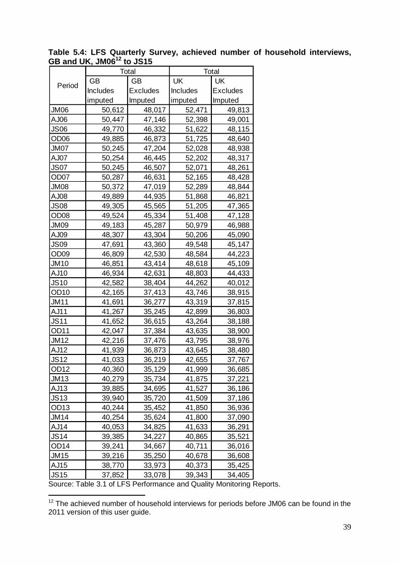
39

Table 5.4: LFS Quarterly Survey, achieved number of household interviews, GB and UK, JM0612 to JS15

Source: Table 3.1 of LFS Performance and Quality Monitoring Reports.

12 The achieved number of household interviews for periods before JM06 can be found in the 2011 version of this user guide.

GB

Includes

imputed

GB

Excludes

Imputed

UK

Includes

imputed

UK

Excludes

Imputed

JM06 50,612 48,017 52,471 49,813

AJ06 50,447 47,146 52,398 49,001

JS06 49,770 46,332 51,622 48,115

OD06 49,885 46,873 51,725 48,640

JM07 50,245 47,204 52,028 48,938

AJ07 50,254 46,445 52,202 48,317

JS07 50,245 46,507 52,071 48,261

OD07 50,287 46,631 52,165 48,428

JM08 50,372 47,019 52,289 48,844

AJ08 49,889 44,935 51,868 46,821

JS08 49,305 45,565 51,205 47,365

OD08 49,524 45,334 51,408 47,128

JM09 49,183 45,287 50,979 46,988

AJ09 48,307 43,304 50,206 45,090

JS09 47,691 43,360 49,548 45,147

OD09 46,809 42,530 48,584 44,223

JM10 46,851 43,414 48,618 45,109

AJ10 46,934 42,631 48,803 44,433

JS10 42,582 38,404 44,262 40,012

OD10 42,165 37,413 43,746 38,915

JM11 41,691 36,277 43,319 37,815

AJ11 41,267 35,245 42,899 36,803

JS11 41,652 36,615 43,264 38,188

OD11 42,047 37,384 43,635 38,900

JM12 42,216 37,476 43,795 38,976

AJ12 41,939 36,873 43,645 38,480

JS12 41,033 36,219 42,655 37,767

OD12 40,360 35,129 41,999 36,685

JM13 40,279 35,734 41,875 37,221

AJ13 39,885 34,695 41,527 36,186

JS13 39,940 35,720 41,509 37,186

OD13 40,244 35,452 41,850 36,936

JM14 40,254 35,624 41,800 37,090

AJ14 40,053 34,825 41,633 36,291

JS14 39,385 34,227 40,865 35,521

OD14 39,241 34,667 40,711 36,016

JM15 39,216 35,250 40,678 36,608

AJ15 38,770 33,973 40,373 35,425

JS15 37,852 33,078 39,343 34,405

TotalTotal

Period

40

Table 5.5: LFS Quarterly Survey, achieved number of person interviews, GB and UK, JM0613 to JS15

Source: Table 3.1 of LFS Performance and Quality Monitoring Reports.

13 The achieved number of person interviews for periods before JM06 can be found in the 2011 version of this user guide.

GB

Includes

imputed

GB

Excludes

Imputed

UK

Includes

imputed

UK

Excludes

Imputed

JM06 116,007 109,086 120,847 113,772

AJ06 115,591 106,321 120,651 111,111

JS06 114,095 104,873 118,920 109,538

OD06 114,442 106,263 119,186 110,835

JM07 115,572 107,126 120,157 111,581

AJ07 115,425 104,696 120,379 109,447

JS07 114,970 104,637 119,605 109,078

OD07 114,562 104,280 119,243 108,747

JM08 114,786 105,524 119,606 110,113

AJ08 113,430 99,433 118,386 104,157

JS08 111,446 101,325 116,222 105,835

OD08 112,618 101,334 117,373 105,900

JM09 111,970 101,075 116,512 105,360

AJ09 109,605 95,767 114,310 100,159

JS09 108,160 96,468 112,784 100,937

OD09 106,112 94,056 110,511 98,237

JM10 106,457 96,889 110,817 101,064

AJ10 106,531 94,061 111,177 98,529

JS10 99,568 87,919 103,943 92,107

OD10 98,801 85,731 102,842 89,560

JM11 97,432 82,763 101,645 86,727

AJ11 96,032 80,069 100,286 84,113

JS11 96,343 82,939 100,543 87,048

OD11 97,950 85,416 102,059 89,328

JM12 98,487 85,630 102,532 89,468

AJ12 98,105 84,124 102,427 88,206

JS12 95,773 82,917 99,901 86,845

OD12 94,378 80,406 98,513 84,350

JM13 94,494 82,219 98,531 85,984

AJ13 93,121 78,994 97,274 82,740

JS13 93,432 82,223 97,380 85,897

OD13 94,826 81,698 98,878 85,435

JM14 95,411 82,706 99,315 86,398

AJ14 94,621 79,818 98,668 83,587

JS14 92,143 77,698 95,950 80,989

OD14 91,953 79,298 95,704 82,717

JM15 92,233 81,356 95,941 84,757

AJ15 91,361 77,816 95,359 81,364

JS15 89,096 75,835 92,784 79,105

Total Total

41

The decline in response rates has been explored in the National Statistics Quality Review : http://webarchive.nationalarchives.gov.uk/20160105160709/http://www.ons.gov.uk/ons/guide-method/method-quality/quality/quality-reviews/list-of-current-national-statistics-quality-reviews/nsqr-series--2--report-no--1/index.html

5.8 QUALITY CONTROL OF FIELDWORK The LFS is a high quality product. This has been achieved over a period of time with methodological research and continued improvements to both fieldwork and management practices. For example, in order to minimise non-response, interviewers call back at non-contactable addresses a minimum of four times, two of which must be in the evening or at weekends. All interviewers have been trained in Achieving Cooperation Training (ACT). Supervision and training are an important determinant of quality control too; the work of all interviewers is regularly monitored in respect of interviewing technique, dealing with the public, response rates, work efficiency, calling patterns (field interviewers only) and the quality of completed work, including the accuracy of coding. Interviewers are provided with both verbal and written feedback on their performance. Where a weakness in performance is identified, additional training and monitoring is carried out. 5.9 NON-ENGLISH SPEAKING RESPONDENTS Measures to meet the Welsh Language Act Since 1985, all sample addresses in Wales are sent advance letters in both Welsh and English. A Welsh translation of the Purpose leaflet is also sent. Where a respondent requests that the interview be conducted in Welsh, arrangements can be made to transfer the household to a Welsh speaking interviewer. However, such requests are rare. Measures to gain response from non-English speakers All face-to-face interviewers are issued with a language identification card, containing a message written in the 22 main foreign languages spoken in Great Britain14. The card is used to identify a time when an English speaking family member or friend can be contacted to explain the survey’s purpose. Where there is no English speaker available, the card also enables interviewers to identify the language spoken so that the interviewer can arrange an interpreter.

14 These languages include: Arabic, Bengali, Chinese (traditional), Chinese (simplified), Czech, Greek, Gujarati, Hindi, Lithuanian, Polish, Portuguese, Punjabi, Romanian, Russian, Serbian, Slovak, Somali, Tamil, Turkish, Urdu, Welsh, Yoruba.

42

SECTION 6 - CODING AND PROCESSING THE DATA

6.1 CODING All coding of data, where required, is carried out by interviewers; some of this is performed using Computer Assisted Coding (CAC) during the interview while the rest is carried out after the interview. The following questions currently require coding and the method currently used is explained:

Variable

Description

Coding method:

BY CAC

DURING

INTERVIEW

by interviewer after interview

CRYO7/CRYSPEC Country of Birth

NATO7/NATSPEC Nationality

NATIDCOD/NATIDO National Identity

ETHO2/ETHDES Ethnicity

RELOCOD/RELOTH Religion

M3CRYO/M3CRYSPEC Country of residence 3 months ago (if outside UK)

M3RESC/M3AREA/M3CTY Place of residence 3 months ago

OYCRYO/OYCRYSPEC Country of residence 1 year ago (if outside UK)

OYRESC/OYAREA/OYCTY Place of residence 1 year ago

WKPL99/WKARBC/ WKTOWN/WKCTY

Workplace of main job

WKPL299/WKTOW2/WKCTY2 Workplace in second job

SMSOC10/SRCHSMSOC/SMOCCT/SMOCCD

Occupation of main wage earner (social mobility)

SUBCODE/SUBJQ Area of study

SNGDEGN/FDSNGDEG/SNGHD/SUBJCTN/FDSUBJ/HDSUBJCT

Subject Area

UGINST/PGINST/FDINST/HDINST Institution studied at

CURCODE/CURSUB Subject of qualification

TSUB4COD/TSUBJ4WK Subject of tuition

43

TIMECODE/TIMEDAYS Time after accident until returned to work

INDD/INDT Industry in main job

OCCT/OCCD Occupation in main job

RDINDD/RDINDT Industry before redundancy

RDOCCT/RDOCCD Occupation before redundancy

INDD2/INDT2 Industry in second job

OCCT2/OCCD2 Occupation in second job

OYINDD/OYINDT Industry in job 1 year ago

OYOCCT/OYOCCD Occupation in job 1 year ago

APPD/APPT Apprenticeship (continuing)

APPIND/APPINT Apprenticeship industry

6.2 DERIVED VARIABLES In order to analyse LFS data, a number of derived variables (DVs) are specified. The survey cannot provide all of the information that users want by asking a simple question, there DVs are created by combining the answers to two or more questions from the questionnaire. These do not vary significantly from year to year, although only those DVs which relate wholly to core data are created each quarter. DVs relating to non-core data are only created in the quarter(s) those non-core questions are included. All DVs are specified for the UK as they are created after the NI data are merged with GB data. Volume 4 contains the latest set of flow diagrams used to specify the current DVs, which can be split into four groups: Person: DVs created for each individual record on the database; Family: DVs created for each family on the database; on a flat file each family

member would carry the same value for each family based DV; Household: DVs created for each household on the database; on a flat file each

household member would carry the same value for each household based DV;

Eurostat: DVs created for each record specifically to meet Eurostat

requirements. These are not currently available to external customers: they are included here for completeness.

44

6.3 DATA CHECKING Whilst some checking is performed in-the-field by the BLAISE survey instrument, other checks are carried out once the data have been received back from interviewers in the field or from the telephone unit. The principles of the checks are to ensure that the data have no duplication of records etc, that the data have the correct household structure, in terms of persons in the household, and that certain key variables have valid values. These checks are important in maintaining the quality of the data. Examples include:

checking that families have been correctly assigned within households by referring to the relationship grid

checking that responses from a previous wave are consistent with the current wave on a number of key variables (eg. AGE, SEX ...). These are known as ‘imputation checks’

country checks to ensure geographies are consistent across variables

checks to ensure each household has a household reference person (HRP)

checks to ensure that there is a record for every member of a household – known as the ‘full house check’

checks to ensure that the household type (HHTYPE6) matches the household composition as defined in the relationship grid

checks on ages for outliers (e.g. very old, old workers etc)

cross checks between variables indicating activity status (e.g. INECAC05 and STATR & INECAC05 and ILODEFR)

.

45

SECTION 7- NON-SAMPLING ERRORS

The following section is drawn from the report ‘Measuring and Improving Data Quality’ by Vera Ruddock published as part of the GSS Methodology Series (no. 14)15. The provision of accurate, timely data which meets the needs of users at minimal cost is at the heart of government statistics. There are two components to accuracy: sampling errors which occur when data from a sample is used to make inferences about the whole population (see section 8) and the so called ‘non-sampling errors’ which affect data from sample surveys, as well as administrative and census data. Non-sampling errors should not be viewed as mistakes, rather they are the result of conscious decisions to produce timely, accurate data at minimum cost. Measuring non-sampling error is much more difficult than measuring sampling error because in many cases the reasons for the non-sampling error are not known, whereas sampling error is a direct result of the survey design and is under the control of the researcher. In some cases it may not be possible to measure non-sampling error or to only give an indication of its possible effect on the survey estimates. Non-sampling errors can also be very expensive to measure. The rest of this section examines how accuracy of survey estimates can be measured and describes the different types of non-sampling error and their occurrence on the LFS. 7.1 MEASURING ACCURACY Users of statistics commonly ask the question ‘Is the estimate accurate?’ The answer to this question influences the value the user attaches to the estimate, and the potential for the estimate to change the user’s beliefs about a given subject. Accuracy is one concept, which defines the quality of a survey estimate. Accuracy reflects the difference between the survey estimate and the population parameter being estimated. The question ‘Is the estimate accurate?’ is only the first part of the underlying question ‘Is the estimate accurate enough for the purpose I want to use it for?’ Discussions of the accuracy of estimates must therefore reflect the context in which they are to be used, but this assessment of the suitability of estimates for addressing specific issues requires some measure of the quality of the data. Accuracy is not usually reported; instead the error in an estimate is described by the bias and variance in that estimate, the two components of the total survey error. Total Survey Error is the inverse of accuracy. A statistic with low accuracy will have high total survey error. Total survey error is measured by the mean square error, which is defined as the sum of all biases and variances: i.e. MSE = variance + bias2

15

http://webarchive.nationalarchives.gov.uk/20160105160709/http://www.ons.gov.uk/ons/guide-

method/method-quality/specific/gss-methodology-series/index.html

46

The biases and variances may be due to sampling error, non-sampling error or both. Reported mean squared errors for survey estimates commonly only include the bias and variance attributable to sampling error. However non-sampling error can lead to biased estimates, for example in surveys people may systematically under report their consumption of alcohol. Similarly slight differences in the way respondents react to different interviewers may lead them to give different answers to different interviewers resulting in interviewer variance. 7.1.1 Bias Sources of bias can be classified into errors of non observation and errors of observation. Errors of non observation include:

coverage error. If the register or sample frame used to select the sample does not represent all the target population then the resulting sample estimate may be biased. For example a random sample of people who are in the telephone directory will exclude both those who:

have no telephone and those who are ex-directory. If the value of a variable being measured in the survey is different for people who are and are not in the telephone directory then the survey estimate will be biased (see Sampling Frames in section 3);

non response. If the people who do not respond to surveys are different from responders then estimates from the achieved sample may be biased estimates of population values - this can be corrected to some extent by weighting the sample.

Errors of observation include:

social desirability effects: an unwillingness of respondents to admit to socially undesirable behaviour. This is most obvious in surveys of sexual experience when men commonly over-report and women under-report the number of sexual partners they have had in their lifetime.

7.1.2 Variance An estimate of the variance of a statistic is based on the variability within the sample, which arises because achieved values differ over the units (e.g. sampled person, interviewers used, questions asked) that are the sources of the error. Sources of variance include:

Sampling variance: In sample surveys only a proportion of the population has been sampled. The sampling variance reflects the fact that the estimate may have been different if a different sample had been selected.

Non-sampling variance: There are a variety of sources of non-sampling variance. For example differences between interviewers may consciously or unconsciously cause variation in the answers given by respondents; this is known as interviewer variance since it is due to differences between interviewers in achieved responses.

47

In the course of designing a survey many decisions are taken which may influence the relative size of different sources of error. These may reduce the bias in an estimate at the expense of an increase in the variance of the estimate. Alternatively survey designs which minimise one source of survey error may lead to an increase in another source of error. For instance, a common trade-off is the issue of whether to allow proxy responses in household surveys. In the LFS adult members of a household are allowed to answer questions on behalf of absent members of the household. This minimises the extent of missing data (item non-response), but the quality of the data from proxy respondents is not always as high as data from the actual intended respondent so respondent error is increased. In contrast to the LFS, proxy responses are not accepted on the Living Costs and Food Survey (LCF), because of the very detailed nature of the survey, the result being a much lower response rate. In some cases the use of proxies may introduce respondent bias into the results if they consistently underestimate variables such as household income, but in others some proxies will underestimate and others overestimate the true value leading to an increase in respondent variance. For more discussion of proxy responses on the LFS, see section 5.5. The following diagram (from Moses) illustrates how bias and precision relate to distinct aspects of sampling procedure.

A Sampling fluctuations Large bias, low precision . . . . ................ . . . . Bias

Population value

B Sampling fluctuations Large bias, higher precision . . . . ........ . . . . Bias

Population value

C Sampling fluctuations No bias, low precision . . . . ................ . . . . Population value

D Sampling fluctuations No bias, higher precision . . . . ........ . . . . Population value

The dots in the diagram represent estimates of the population value derived from repeated application of the given survey procedures i.e. they represent the sampling distribution of the estimates and their mean is the expected value. The population

48

value is what the survey is trying to estimate. The terms ‘large’, ‘low’ etc are, of course, relative. It can be taken that (D), which is unbiased and relatively precise, is the ideal, whereas (A) is to be avoided. In practice the choice is not as simple as this, and there are circumstances in which a sample designer might be prepared to tolerate some bias if precision could markedly be increased. 7.2 TYPES OF NON-SAMPLING ERROR Non-sampling errors - bias and variance - can be classified into three broad categories: 1. a) errors of non observation, which can be broken down into:

coverage error

non-response error 2. b) measurement errors, of which there is:

interviewer error

respondent error

instrument (or questionnaire) error

mode error 3. c) processing errors, consisting of:

systems error

data handling error Each of these is described below, in relation to the LFS. 7.3 ERRORS OF NON-OBSERVATION 7.3.1 Coverage error Coverage error is the error which arises because some units are either excluded or duplicated on the sampling frame used to identify members of the population of interest. A sampling frame has 3 elements :

a list representing all elements in the target population;

further characteristics of these elements (auxiliary information);

the probability of selecting each element on the frame. The coverage ratio is the proportion of the target population included on the sampling frame. It gives an indication of the level of possible under-coverage, but does not measure the impact of under-coverage on survey estimates. Biased estimates can be caused by under coverage and duplicate listings while increased variance of estimates can be caused by inclusion of non population elements in the list and errors in auxiliary information.

49

Coverage bias and variance can be measured by comparing data on the sampling frame with external data and by using special data collection procedures incorporated into the survey. Coverage error is minimised by using accurate up-to-date frames. Out of date lists can have the following impact on data quality:

bias in survey estimates if new elements differing from elements already on the list have not been added to the list;

increase in the variance of estimates if auxiliary information used for stratification or estimation is inaccurate, or it is discovered during a survey that sampled elements should not be on the list;

reduction in survey response rate if elements are untraceable and it is not possible to ascertain that the elements are either old elements which should not be on the sampling frame or elements with inaccurate addresses which cannot therefore be traced.

For more detail on the LFS sampling frame and the way it is kept up-to-date, see section 3 of this volume. 7.3.2 Non Response error There are two types of non-response error:

Unit non-response: failure to obtain any of the substantive measurements from the sampled unit (the unit response rate is the proportion of the sampled population responding to a survey);

Item non-response: failure to obtain specific items of information from an otherwise responding unit.

Non response bias in an estimate has two components:

the proportion of the sample responding to the particular question;

the difference between the true answer to a question in respondents and non respondents.

Even if the response rate is high, large differences in the true answer to a question in respondents and non respondents may lead to substantial non response bias. Non response can reduce the precision of survey estimates - this can be pre-empted at the design stage by increasing the size of the survey sample. Unit non-response There are four sources of information about non-respondents which can be used to examine the existence of unit non-response bias:

information on the sampling frame;

census records for responding and non responding units which can be matched to the sampling frame;

information collected by interviewers in a follow up survey of non respondents;

in panel surveys, information collected from respondents in earlier waves of the survey.

Strategies for minimising unit non-response include:

50

interviewer training to reduce the number of refusals - interviewer training on the LFS is rigorous and all interviewers work solely on the LFS.

encouraging interviewers to call on weekday evenings and at weekends - the timings of the LFS face-to-face and telephone interviews are managed in order to maximise the chances of gaining a response from a household, so much of the interviewing is done in the evenings.

sending an informative well designed advance letter in interview surveys – households chosen for the LFS are sent a letter before their first interview which explains the background to the LFS, that the survey is voluntary and that responses will be treated as confidential, and gives a rough idea of when the interviewer is likely to call.

reducing the burden on the potential respondent - the length of the questionnaire is reviewed regularly in order to keep the interview length down.

offering incentives to respondents - while respondents to the LCF are given a monetary reward for completing a diary of their spending, no incentives or rewards are offered to LFS respondents.

sending follow up reminders for postal questionnaires and making repeat calls in telephone/face-to-face questionnaires. Face-to-face and telephone interviewers will make a number of attempts to contact a household before it is treated as non-response.

For more information on LFS interviewing, see section 5. Weighting is also used on the LFS (see section 10) to compensate for unit non-response. The complicated population weighting allocates a weight to each individual, ensuring that the respondents are representative of the population as a whole, in terms of age, sex and region of residence. It also converts the sample estimates into estimates expressed in terms of the population. Item non-response An indication of the level of item non-response bias can be gained by comparing the characteristics of people responding and not responding to a particular question. Strategies for minimising item non-response include :

clear question design;

computer assisted modes of administering interviews to reduce routing errors and identify possibly erroneous data in the course of the interview - all LFS data is collected by laptop or PC, allowing a number of data checks to take place during the interview.

On the LFS, imputation (see section 12) is used to estimate missing items on a questionnaire so that the potential bias in estimates due to item non response may be reduced. 7.4 MEASUREMENT ERROR There are four types of measurement error:

interviewer error arising from both conscious and unconscious differences in the way interviewers administer a survey, and also from the reactions of respondents to different types of interviewers;

51

respondent error arising from the inability or unwillingness of a respondent to produce a correct answer;

instrument error which reflects the effect of question wording, response categories and form design on responses; and

mode error which describes the effect of different methods of administering a questionnaire on the recorded responses.

Measurement bias can only be accurately measured in record check studies where the true value of a response is matched to the survey response. An indicator of measurement bias can be obtained from split sample studies where one component of the survey design is varied across subgroups of the sample. Different subgroups may :

receive different questionnaires to investigate instrument bias; or

have their interview administered in different ways, for example some may receive a face-to-face interview and others may fill in a self completion questionnaire to investigate mode bias.

cognitive testing methods which ask respondents to questionnaires why they gave certain answers and attempt to understand the process leading to a response may be used to study respondent and instrument bias.

measurement variance is important in interviewer surveys. High interviewer variance can have a large effect on the precision of survey estimates.

The different types of measurement error can be minimised using a variety of methods:

interviewer error is minimised by thorough ongoing interviewer training and the use of small interviewer quotas to reduce the influence of interviewer variance on the precision of survey estimates;

respondent and instrument error are minimised by careful question testing – new questions for the LFS are generally tested twice and feedback from the interviewers taken into account before the questions become part of the survey.

mode error is minimised by using appropriate methods to collect data on sensitive questions - it is hoped that response bias on LFS earnings questions can be evaluated and perhaps reduced by asking respondents to check documentary evidence such as a payslip and recording whether such evidence was provided. There are also small but noticeable differences in the information collected by face-to-face interviewers and by telephone interviewers. Although some of the difference can be explained by respondents getting used to the interviewing process with each successive quarter’s questioning, some of the difference is also due to the mode effect and it is difficult to disentangle the two causes. Estimates of employment are about 1 per cent lower, on average, in first interviews (face-to-face) than in subsequent interviews (telephone). However, as the survey design has not changed in recent years the estimates are consistent over time, and therefore estimates of change are unaffected by these effects.

52

7.5 PROCESSING ERROR There are two types of processing error: systems error and data handling error. Systems errors are errors in the specification or implementation of systems needed to carry out surveys and process results; system errors on the LFS can creep in when derived variables are specified and/or amended. Data handling errors are errors in the processing of survey data. There are various sources of data handling error:

Data capture Information recorded on a paper questionnaire may be inaccurately converted to a format which can be interpreted by a computer. On the LFS, data capture is automatically incorporated into computer assisted interviewing modes of data collection, but interviews themselves may mis-key answers. This type of error on the LFS is minimised by using mainly computer-assisted data capture with inbuilt checks.

Data transmission Electronic data on interviews may be lost in transit between the field and the head office but this can be minimised by using an effective case management system to track the progress of individual packets of data.

Editing Errors may be introduced when raw survey data is transformed into a dataset which can be used for producing estimates. These errors can be minimised by:

incorporating survey edits into computer assisted interviews so that the respondent can be asked about suspect responses - the method used on the LFS;

involving subject matter specialists so that the edits are appropriate for the data;

testing program code used in editing.

Coding Coding is the transformation of textual open-ended responses to survey questions into categories to be used in data analysis. Coding systems may be manual, computer assisted - where the computer suggests a list of possible codes to the human coder, or computer automated. The last two of these methods are used on the LFS, particularly for industry and occupation coding.

Individual coders may unconsciously show preferences for particular codes. The impact of these individual biases in the codes allocated by coders on survey estimates may cancel out, however although the survey estimate may not be biased, the variance of the estimate may be increased. If the individual biases do not cancel out then the coding error will introduce bias into the survey estimate. These types of errors can be minimised by effective training of coders in using the coding system.

Weighting and imputation The use of inappropriate methods of weighting and imputation may introduce errors into survey estimates. See section 10 for more detail on LFS weighting and section 12 on imputation.

53

SECTION 8 - SAMPLING ERRORS AND CONFIDENCE INTERVALS

Surveys are prone to errors arising from a number of sources and processes. Frequently a distinction is drawn between non-sampling errors and sampling errors. Sampling errors result from the fact that only a sample of the population has been selected, and a different sample would probably produce a different estimate. Non-sampling errors are covered in section 7 of this volume. They measure error that is not due to random sampling and would remain even if every case in the population was sampled. Sampling errors relate to the fact that the sample chosen is only one of a very large number of samples which might have been chosen. It follows from this that an estimate of, say, the number of people in employment, is only one of a large number of such estimates which might have been made. The probable spread of these different estimates can be thought of as the precision of our estimate of the number of people in employment. Greater precision is associated with a relatively narrow spread. In general, a larger sample size equates to a smaller spread of probable estimates and therefore greater precision. 8.1 MEASURING PRECISION USING STANDARD ERRORS A measure of the spread of different probable estimates is provided by their standard error. This is the standard deviation (the average amount of variation about the average) of the estimates which would have arisen from the different samples which might have been taken. The smaller the standard error, the more precise is the estimate. The size of standard errors is determined by a number of factors, including the sample size and the variability of the population from which the sample is drawn. The third important factor in determining the size of standard errors is the sample design. Standard errors calculated from simple random samples will differ from those calculated from more complicated sample designs, such as clustered or stratified samples. A useful benchmark to assess the relative magnitude of a standard error is to calculate the ratio of the standard error derived from a particular (complex) sample design with the standard error that would have arisen from a simple random sample of the same size. This ratio (of the standard errors) is the design factor. It indicates the relative gain (or loss) in the estimate of standard error which results from the use of a particular complex sample design compared to a corresponding simple random sample. A design factor (or DEFT) of, say, 1.20 indicates that the standard error of the estimate in question is 20% greater than would have been the case for a simple random sample of the same size. The design factor (DEFT) should not be confused with the design effect (DEFF); the design effect is the design factor squared and is calculated by the ratio of variances instead of standard errors. In the case of the LFS sample design, there is a clustering effect. This reflects the fact that addresses are sampled, but that results are shown for individuals. For example, ethnicity is particularly clustered, since it is likely that all members of a household living at a particular address will share the same ethnicity. This results in,

54

for example, the design factor for the ’Asian or Asian British’ group being 1.58, which is higher than for the other ethnic groups because of the tendency for Asian ethnic groups to live in large households. The design factor for part-time employees on the other hand is 0.97, reflecting the fact that part-time employee status is not clustered within a household. By itself, clustering would tend to increase the design effect of LFS estimates. However, the LFS uses a systematic sample of addresses ordered by postcode sector (see section 3). This means that the sample will be representative geographically, which will reduce standard errors. This effect is referred to as implicit stratification (as opposed to explicit stratification, where a population is split into sub-groups and a sample is taken from each sub-group). The weighting process used on the LFS will also reduce standard errors because it ensures that the weighted dataset is representative of the population (see section 10).

8.2 CALCULATING CONFIDENCE INTERVALS While the standard error and the design factor of estimates are important items of information in their own right - because they indicate the precision of the estimate and the relative efficiency of the sample design in deriving the estimate - they also form the basis for calculating confidence intervals associated with particular estimates. A 95% confidence interval for a population estimate is ±1.96 standard errors around the estimate calculated from the sample. The tables in Annex B to this volume of the LFS User Guide, list a number of estimates from the January 2015 to March 2015 LFS, the standard errors and other related statistics. The standard errors presented in the Labour Market Statistics statistical bulletin, LFS Quarterly Supplement and Annex B are shown for the UK and are calculated using UK design factors. For example, in January-March 2015 the proportion of people in the UK aged over 16 who were estimated to be economically active was 0.63. The number of people aged 16 and over in the UK sample was 73,768 and since the design factor was 0.97, the standard error was 0.0017, calculated as: SE (given LFS design) = Design Factor * SE (assuming simple random sample)

= DEFT * n

pp )1(

= 0.97 * 768,73

37.0*63.0 = 0.0017

Hence a 95% confidence interval would be:

0.63 ± (1.96 * 0.0017) = 0.63 ± 0.0033 = (0.6267, 0.6333) What this means in practice is that in 19 samples out of 20 we would expect the true economic activity rate to lie within the 95% confidence intervals constructed. Only in 1 in 20 samples would we expect the true value of the economic activity rate to be outside the confidence interval around the LFS estimate.

55

The standard error of the total of the estimate is approximately the standard error of the proportion (or rate) multiplied by the population aged 16 and over:

0.0017 * 51,857,166 =88,157 and so the 95% confidence interval for the number of economically active people aged 16 and over would be:

32,818,976 ± 172,787 Note that this method for constructing standard errors for totals can only be used when the base (the total the proportion is based on) is not itself a survey estimate. In practical terms, this means that this method should only be used when the base is a weighting category or a combination of weighting categories – see section 10.2, and is inappropriate when using the income weight – see section 10.5. We use 95% confidence intervals primarily because they are widely used within ONS and elsewhere; they are something of an industry standard. However, other confidence intervals are equally valid, and might help users appreciate the fact that LFS estimates are always subject to error. 8.3 CALCULATING LFS STANDARD ERRORS & CONFIDENCE INTERVALS The standard errors of the UK LFS estimates shown in Annex B are produced using a linearised jackknife approach in order to account for the impact of the calibration weighting on the variance of estimates - calibrated variances will tend to be smaller than non-calibrated variances because calibration ensures that estimates are representative across calibration categories16. Paired addresses (sorted by wave, quarter, quota, week and address number) are used as stratifiers and the address is the primary sampling unit (PSU). This is also the method used for standard errors produced for the first release. It does not take into account the impact of seasonal adjustment on standard errors. The design factors given in the appendix can be used with the formula given in section 8.2 to generate standard errors for key labour market estimates. If other estimates are required, users may wish to calculate their own standard errors. In this case, complex survey commands in statistical software packages can be used – this will account for the survey design but will not account for the reduction in standard errors resulting from calibration weighting, and so this method is likely to produce conservative standard errors. The address identifier should be used as a cluster variable, as LFS person responses are clustered within addresses. Because the LFS uses systematic sampling, a good geographic coverage is ensured – this is called implicit stratification (see section 8.1). This can be accounted for by using a low level of geography as a stratum variable.

16

Holmes, D. J. and Skinner, C. J. (2000), “Variance estimation for Labour Force Survey estimates of

level and change”, No 21, Government Statistical Service Methodology Series, available at http://webarchive.nationalarchives.gov.uk/20160105160709/http://www.ons.gov.uk/ons/guide-

method/method-quality/specific/gss-methodology-series/index.html

56

In the case of totals based on small sample sizes, a useful approximation for the 95% confidence interval of an estimate of ‘M’ is:

1000

92.1**1000

MM

The derivation of this formula is given in appendix B. It implies that, for an LFS estimate of 20,000, the confidence interval will be approximately –

1000

92.1*000,20*1000000,20 = 20,000 ± 6197.

This method may not work for estimates of total employed and total inactive as these tend to have very low design effects due to the effect of post-stratification. 8.4 STANDARD ERRORS AND CONFIDENCE INTERVALS OF ESTIMATES OF CHANGES In the same way that standard errors relating to quarterly estimates of means or proportions can be calculated, so standard errors can be calculated which relate to changes. Standard errors (and hence confidence intervals) of estimates of changes are

calculated as follows; where 1tp is the relevant proportion at time 1, 2tp is the

relevant proportion at time 2, k is the sample overlap (approximately 0.8 for successive quarters) and r is the correlation coefficient -

rkpp

ppkrpppp

tt

tttttt

1varvar

2

varvar2varvarvar

21

21

2121 (1)

2121 var tttt ppppse (2)

This is the method used for standard errors for the main labour market release, with correlation coefficients calculated as detailed in Holmes and Skinner (2000). With the

additional assumption that 21 varvar tt pp it can be simplified further -

Since n

ppdeftp

)1(*var 2

, if 21 varvar tt pp then –

npprkdeftpp tt /)1(*)1(2*var 2

21 (3)

npprkdeftppse tt /)1()1(2*)( 21 (4)

A few key labour market standard errors for two-quarter changes in totals are given in the table below, calculated using formulae (1) and (2) :

57

Table 8.1: Standard error for two-quarter changes for economic activity status, Q1 2010 to Q2 2010

Q1 2010 to Winter Q2 2010 (UK) (not seasonally adjusted)

Quarterly correlation

Quarterly change

Standard error of change in

level

Economically active 0.8 120,526 61,886

Employed 0.8 188,247 65,663

ILO unemployed 0.54 -67,721 42,879

Economically inactive

0.8 -21,544 61,886

As the SE for change in total employment is given as 65,663; then a 95% confidence interval for the change of +188,247 can be calculated as:

128,700 188,247 65,663) * (1.96 188,247

8.5 RELIABILITY THRESHOLDS It is the nature of sampling variability that, when estimating population sizes, the smaller the group whose size is being estimated, or from which an estimate is being derived, the less precise that estimate is. Put another way, the size of the standard error increases with the level of the estimate, so that the larger the estimate the larger the standard error. But the larger the sample estimate, the smaller will be the standard error in percentage terms (relative standard error being the standard error as a percentage of the estimate). Thus, larger sample estimates will be relatively more reliable than smaller estimates–an estimate of 500,000, while having a standard error of 13,800 will have a relative standard error of 3%, compared with an estimate of 25,000 which has a standard error of 3,100 and a relative standard error of 12%. This is because larger estimates will be based on more cases. Before 2005, quarterly LFS estimates of under 10,000 were not published as they are likely to be unreliable. Although this publication policy changed in 2005 (as a result of the Freedom of Information Act), the unreliability of these LFS estimates did not. It is suggested that the 10,000 threshold is used as a guide to identify which cells will be subject to high sampling variability. Users are advised that estimates below 10,000 are subject to a high degree of sampling variability and should therefore be treated with caution. The 10,000 threshold equates to a sample size of about 25 and a relative standard error of about 20%. The graph below shows how, for different values of p (i.e. for different proportions of the population), the standard error rises at a much steeper rate when the sample size is less than 30 - very small estimates, those based on fewer than 25 cases, are subject to such high standard errors (relative to the size of the estimate) as to detract seriously from their value, which is why the reliability threshold is recommended to be around that level. That said, a relative standard error of 20% is a somewhat arbitrary cut-off point, the Australian Bureau of Statistics uses a publication threshold of a relative standard error of 25%. A sample size of fewer than three is potentially disclosive so this information is suppressed even under the Freedom of Information Act.

58

Estimates of 10,000 have associated 95% confidence intervals of 10,000 ±4,000 -so particular care must also be taken in using estimates of change from period to period for these estimates. For example, the estimated size of a particular group may be unchanged at 10,000 in two successive quarters but, because of the unreliability of these estimates, we cannot safely conclude that the true size of the group has not changed between those quarters. A variable with a quarterly correlation of 0.9, would have a 95% confidence interval for its quarterly change of 0 ± 3000. So, even if the estimate does not change, the true size of the group could have changed by up to 3000 in either direction. 8.6 RELIABILITY THRESHOLDS FOR EARNINGS DATA Earnings data from the LFS are based on only a part of the sample and so are subject to a different reliability threshold. Earnings may be regarded as a continuous rather than a discrete variable; other things being equal, estimates of continuous data are more precise than estimates of discrete data. So although earnings estimates are based on a smaller sample size than most other estimates, LFS estimates of gross average hourly or weekly earnings for all employees are usually more precise (in terms of relative standard error) than an estimate of, for example, the number of employees. However, to set an alternative reliability threshold for estimates of earnings (as opposed to estimates of numbers of people), based on maintaining a relative standard error of less than 20% is problematic for two reasons. Firstly, the standard errors of estimates of continuous variables like earnings are not determined by the estimates themselves (unlike estimates of numbers of people), so an appropriate threshold for one continuous variable will not work for another, even if their mean values are the same.

Variation in standard errors according to changes in p and sample size (n)

0.00

0.05

0.10

0.15

0.20

0.25

5 10 20 30 40 50 60 70 80 90 100

Sample size (n)

standard error p=0.1, for example self-employed

p=0.2

p=0.3

p=0.4

p=0.5, for example employees

59

Secondly, standard errors of earnings estimates are dependent on the degree of variation within the sample. Thus, an estimate of earnings of a sub-group whose earnings are similar will have a relatively small standard error, whereas a group with more variable earnings will produce an estimate with a larger standard error, though both estimates may take the same value and be based on similar sample sizes. Estimates derived from discrete variables are affected by variability in a different way since, essentially, there are just two outcomes - whether a respondent is in a specified group or not. Because of these issues, we recommend adopting a conservative approach by treating these estimates as though they were based on discrete counts. The recommended threshold when using LFS earnings data is set at 60,000 people for estimates based on Wave 5 only (for quarters prior to Spring 1997), and at 30,000 for estimates based on combined Waves 1 and 5 (for Spring 1997 onwards). As with non-earnings tables, it is suggested that these thresholds are used as a guide to identify those cells which are subject to a higher degree of sampling error, that a similar warning advising of this is added to the cells in question, and that they should be treated with caution. Both of these recommended thresholds equate to a sample size of about 25 respondents, as before. Much output from earnings analyses is in the form of means or proportions, so users need to be aware of the size of the population on which such estimates are based. 8.7 RELIABILITY THRESHOLDS FOR ANNUAL LFS DATA For Annual LFS data prior to 2000-01 when the survey was enhanced, estimates of fewer than 6,000 are likely to be unreliable. However, since 2000-01, the nature of LFS enhancement has meant that some areas have seen a very large increase in sample size, and others a very small increase or none at all. This means that a single threshold for all areas is no longer appropriate. Following the enhancement in 2000-01, each area in England was allocated to one of three threshold bands – 2,000, 4,000 or 6,000. Annex D of Labour Force Survey User Guide Volume 6 Local Area Data, contains details of how this allocation has been made. For Wales, from 2001-02, each Unitary Authority was allocated to one of four threshold bands - 1,000, 2,000, 3,000, or 4,000. Similarly for Scotland, from 2003-04 each Unitary Authority was given its own threshold ranging from 1,000 to 5,000.. It has long been known that the design effects for ethnic group and for totals segregated by ethnic group are substantially greater than those for most other groups. Following an analysis of the variation in design effects between different ethnic groups and different local areas in England, it is recommended that for most ethnic estimates a single multiplier of 2.5 is applied to the general thresholds. A larger multiplier of 3.5 is recommended for totals of individual minority ethnic groups (e.g. the multiplier of 3.5 would apply to the total Indian adults in Birmingham, whereas a multiplier of 2.5 would apply to the total employed Indian adults in Birmingham). A separate analysis for the Welsh Local Labour Force Survey recommended a multiplier of 4.0 in Cardiff and 2.5 for the rest of Wales.

60

SECTION 9 – NON RESPONSE

This section looks firstly at the results from the Census Non-Response Link Study (CNRLS) on the LFS and then at question specific non-response. 9.1 THE 2011 CENSUS NON-RESPONSE LINK STUDY

Since ONS carry out both the Census and the LFS, a study could be carried out, which involves linking census records with the LFS wave 1 cases (in England and Wales)17 that were sampled between March and July 2011 (in Q1 and Q2). This allows a comparison to be carried out on the characteristics of survey respondents and non-respondents, which enables non-response bias to be estimated. Methods of non-response adjustments could then be evaluated to see whether a non-response weight should be introduced on the LFS. Similar work was carried out following the 1971, 1981, 1991 and 2001 census18 , for these periods, it was found that the addition of non-response adjustment to the existing weighting methods only had a negligible effect on estimates and therefore wasn’t implemented. The results of the census non-response link study can be found in the paper “Non-response weights for the UK Labour Force Survey? Results from the Census Non-response Link Study”. http://webarchive.nationalarchives.gov.uk/20160105160709/http://www.ons.gov.uk/ons/guide-method/method-quality/specific/labour-market/articles-and-reports/index.html

For the 2011 CNRLS, 12,790 households from wave 1 LFS were successful matched to the census records, of these: 62.2% co-operated, 11.6% were non-contacts and 26.2% were refusals. Four logistic regression models were used in the study (univariate model (ethnicity based model), multivariate, tree and quality-check). Details of these models and the results can be found in the report. The conclusion of the study was not to introduce a non-response weight on the LFS at this time, as:

a) non-response adjustments have a negligible impact on estimates for the key publication groups explored, except for Ethnicity. However, while the impact on levels within minority ethnic groups is notable, the impact on rates is negligible.(The number of respondents in ethnic groups other than “White” are rather small, which means that the calculated factors from the CNRLS data may not be very reliable. In the “white ethnic group” non-response adjustment had no impact).

b) response rates have continued to decline which indicates that the response process isn’t stable as shown in section 5 of this user guide and in the PQMs. This can also be seen when comparing the response rates in 2001 and 2011 as in 2011 response rates of unemployed (62.1%) were higher than the employees (61.3%) whereas in 2001 response rates were higher for employees (81.1% compared to 74.6%) as shown in the CNRLS report.

17 Linked census-survey data from Scotland were unavailable at the time of the analysis. 18 Information on the 2001 census linked study can be found in the 2011 version of this user guide.

61

9.2 QUESTION SPECIFIC NON-RESPONSE Sometimes data for a particular question is missing from the results because respondents who are routed to the question do not respond. The figures in table 9.1 represent the number of people who did not answer particular questions as a percentage of those who were routed to the question. Table 9.1 Question specific non-response rates

Variable JM15 AJ15 JS15

EVERWK (Whether ever had a paid job)

0.05 0.04 0.05

EVEROT (Paid or unpaid overtime)

0.17 0.15 0.15

FTPTWK (Whether working FT/PT)

0.08 0.08 0.08

ILLWK (Whether off sick or injured in ref week)

0 0 0

SECJOB (Second job)

0.04 0.04 0.05

Users should be aware of this when undertaking analysis. To conclude, various strategies are available to weight survey data to take account of non response. A census based weighting scheme is one approach. ONS currently uses another approach, a population weighting procedure, which involves weighting data to sub-regional population estimates and then adjusting for the estimated age and sex composition by region. When evaluating whether additional information might improve the performance of a population weighting methodology, it is important not to lose sight of issues such as the availability of up-to-date population data at the sub-regional level and the relative transparency of the method.

62

SECTION 10 - WEIGHTING THE LFS SAMPLE USING POPULATION ESTIMATES The LFS collects information on a sample of the population. To enable us to make inferences from this sample to the entire eligible population we must weight the sample data. This entails assigning each responding or imputed case a weight, which can be thought of as the number of people in the population which that case represents. These weights are calculated such that they sum to a set of known population totals, and the weights of an entire dataset will sum to the eligible population of the UK. Population weighting serves several purposes. It ensures that estimates reflect the sample design so that cases with a lower probability of selection will receive a higher weight to compensate. It also compensates for differential non-response among different sub groups in the population, and as such should help guard against potential non-response bias. The use of weights also allows totals, as well as means and proportions, to be estimated easily; and weights may reduce standard errors when the calibration model is included in the variance estimator. It is therefore important to use the weights when doing most types of analysis on LFS datasets. Failing to do so may introduce bias because the sample design will not be taken into account – for example, over-75s will be under-represented, as they are under-sampled. Not using the weights will also result in estimates that are subject to more non-response bias and will make it difficult to estimate totals. The person-weight variable on LFS datasets is usually named ‘pwtXX’, where ‘XX’ refers to the year in which the population totals were projected (see section 10.3). This is the main weight used for inference to person-level population characteristics such as economic activity rates and totals. A household weight and an income weight can also be found on some datasets and may be more appropriate for some types of analysis; these are described briefly in sections 10.4 and 10.5. 10.1 CALIBRATION WEIGHTING THEORY

The LFS uses calibration weighting to assign a calibration weight kw to each

responding individual k. These calibration weights are set to sum to a set of calibration totals within calibration groups – for example, the weights of all 18-year old males in an LFS dataset (a calibration group) will sum to the population total of eligible 18-year old males in the UK (a calibration total) at the time the survey was taken. Calibration weighting typically involves calculating a design weight, making adjustments for non-response, and finally calibration to population totals. The design

weight kd for each individual k is calculated as the inverse of the probability of

selection kp , so that individuals with a lower probability of selection receive a higher

design weight.

63

kk pd /1

It is possible to modify the design weight by non-response factors in order to account for some sub-groups being less likely to respond than others. Non-response factors are not currently used on the LFS but they may be introduced in the future. See section 9 for more details about non-response. It is desirable for the calibration weight to be as close as possible to the design weight, in order to properly reflect probabilities of selection. The calibration weights

kkk gdw , nk ,....,1 are calculated to minimise the sum of the distances between

the kd and the kw , subject to the calibration constraints (ie summing to the known

totals). In summary - the calibration weight is calculated to sum to calibration totals within calibration groups while minimising the adjustment to the design weight. 10.2 CALIBRATION WEIGHTING ON THE LFS The LFS assigns a calibration weight to all responding or imputed individuals, but does not assign a weight to individuals whose economic activity is unknown (so non-responders do not get a weight). Standard LFS practice in the case of individuals dropping out between waves is to roll their data forward by one quarter – this is a form of imputation, and these individuals receive a weight. LFS design weights are typically constant, as in most cases the LFS sample design ensures an equal probability of selection – see section 3. There are three exceptions to this –

- A different sampling fraction, and therefore a different design weight, is used in Northern Ireland.

- From Q3 2010 onwards, over-75s are only interviewed in Wave 1 (see section 3.4.1 for more details). Their probability of selection is therefore lower and their design weight is increased to compensate.

- From Q3 2010 onwards, where multiple households are resident at a sampled address, only one household is interviewed (see section 3.3.1 for more details). The probability of selection for households in multiple-household addresses is therefore lower and their design weight is higher.

These design weights are then calibrated to sum to population totals using the theory outlined in 10.1. Three sets of calibration groups (called partitions) are used, so that each individual is in three separate calibration groups. Recall that, within each calibration group, weights will sum to population totals. The calibration groups used are – Partition 1: Individual Local Authority Districts There are 433 local authorities used in the weighting, meaning there

are 433 calibration groups in this partition.

64

Partition 2: GB/NI by sex for the ages 0-15, 16, 17, 18, 19, 20, 21, 22, 23, 23, 24 and

25+ This partition is a cross-classification, so that age-bands within sexes and GB/NI are used to form calibration categories. As there are 12 age groups, two sexes and two countries in this partition, there are 12*2*2 = 44 calibration groups.

Partition 3: Male/Female by Government Office Region (GOR) and Age-Groups - GOR: Tyne and Wear Rest of Yorkshire and Humberside Rest of North South and West Yorkshire Rest of North West West Midlands Metropolitan County East Midlands Rest of West Midlands East Anglia Greater Manchester and Merseyside Inner London Outer London South West Rest of South East Strathclyde Rest of Scotland Wales Northern Ireland Age groups: 0-4 5-9 10-15 16-19 20-24 25-29 30-34 35-39 40-44 45-49 50-54 55-59 60-64 65-69 70-74 75-79 80+

Like partition 2, this partition is a cross-classification, so that age-bands within government office regions and sexes are used to form calibration groups. As there are 18 regions, 17 age-bands and two sexes in this partition, there are 18*17*2 = 612 calibration categories.

There are therefore 612 + 44 + 433 = 1089 calibration groups, and each responding/imputed individual will be in three of them. For example, a 24-year old man in Cardiff would be in the Cardiff calibration category in partition one, the 24-year old male category in partition two, and the Welsh 20-24 year old male category in partition three. The weights of all calibration categories will then sum to corresponding population totals – for example, the weights of all responders in the Welsh 20-24 year old male calibration category will sum to the Welsh 20-24 year old male population total. The LFS is calibrated using Statistics Canada’s Generalised Estimation System (GES) software, a set of programs designed for calibration weighting. Prior to 2007/8, a raking ratio method was used instead. Raking ratio sets the weights to sum to the calibration totals for each partition in turn – the first stage corrects for partition one, the second for partition two, and the third for partition three. This is then repeated iteratively until the weights sum (sufficiently closely) to all population totals in all three partitions. This method was replaced by GES in 2007/2008 and GES is viewed as more statistically robust and efficient, calibrates to all partitions simultaneously, and allows good variance estimates. GES was used to re-weight back to 1991/1992, so all post-1992 LFS datasets now available will have a weight calculated using GES.

65

The 2011 census resulted in revisions to ONS population estimates, and in 2014/2015 a re-weighting program was carried out to re-weight historical datasets to updated population totals. 10.3 POPULATION TOTALS AND RE-WEIGHTING The LFS weighting methodology requires estimates of the number of people in LFS-defined households19 for each local authority, with a five-year age-breakdown by sex. Population weighting totals are derived from published population estimates and population projections. All population projections (and estimates) are based, directly or indirectly, on the decennial Census of Population, and use additional information from the NHS Central Register for internal migration, the International Passenger Survey for international migration flows, and registration data for births and deaths. See the Quality Monitoring Information (previously, Summary Quality Reports) for Mid-Year Population Estimates and National Population Projections for more details20. Projections use a variety of assumptions about the rates at which the components of population change will evolve. A number of adjustments are made to the published population estimates by local authority and national population projections data to provide estimates of the number of people in LFS-defined households:

(i) Population projections for local authorities are produced by rolling forward a five-year average growth rate (between estimates) for each LAD, then constraining to the published national population projections.

(ii) Estimates of communal establishment population (that is, those excluded from the LFS-defined population) have been made by assuming that the percentage of people in communal establishments was the same (by quinary age band, sex, and region) as it was in the results of the 2011 Census. Hence, for example, as the number of old people changes, the number of old people in institutions changes in line. Then the LFS-defined population is calculated by subtracting the estimate of communal establishments from the total population figures. See section 3.1.2 on Communal Establishments for more details.

(iii) Monthly estimates are produced from the LFS-defined annual population totals - the mid-year estimate/projection less the communal establishment population - by simple linear interpolation.

Re-weighting exercises give the opportunity to use the most up to date population estimates as a part of LFS weighting. In the interests of timeliness, population projections are used to generate the initial population totals for weighting. Population estimates are published one year following the reference date and it is desirable to re-weight to the resulting LFS-defined population totals g iven by these published estimates. Re-weighting consists of re-calibrating historical data, which had initially been weighted to population projections, to newly available population estimates, and then re-projecting into the future. The year in which the population projections have been updated using the most recent population estimates is reflected in the

19

Household residents and NHS staff and students 20

http://www.ons.gov.uk/ons/rel/pop-estimate/population-estimates-for-uk--england-and-wales--

scotland-and-northern-ireland/mid-2014/index.html

66

weight variable – for example, ‘pwt14’ is based on projecting from 2014 population estimates. A 2010 dataset with ‘pwt14’ is therefore weighted to 2010 population estimates calculated in 2014. 10.4 THE LFS EARNINGS WEIGHT Earnings data are collected at Wave 1 and 5 interviews only (before Spring 1997 at Wave 5 only). A separate weight is needed for analysis because data are only collected at two of the five waves - using the normal person weight would be inappropriate, as the weights would sum to considerably less than the relevant population total. During 1998, income weights for Northern Ireland data were added to existing datasets so that it is possible to analyse earnings data at UK level from Winter 1994/5 onwards. However, the weighting exercise is restricted to employees' earnings, and people with a very high income (over £3500 gross per week) are treated as outliers and do not receive an income weight. Individuals where data is brought forward from a previous quarter will also not receive a weight (because the questions are only asked at waves 1 and 5). The aim of the income weight is to allow inference from the income data to the entire target population. This target population is different to the target population which the normal weight refers to because only employees are eligible for earnings questions. The aim is therefore to weight the earnings data to allow inference to the UK employee population. The best source of information of the size of sub-groups in this employee population is considered to be the full LFS dataset, containing all five waves of data. The weighting procedure therefore attempts as far as possible to replicate the results from the employees in waves 1-5 of the LFS in the weighted earnings data, and as such can be thought of as a form of two-phase weighting. It is worth noting that as the total size of the target (employee) population has to be estimated from LFS data, standard errors will be larger than those from the main LFS. This is because the population totals used in the weighting are themselves estimated from the survey. A small number of variables that are likely to be important determinants of income are used to form calibration categories. GES is used to calibrate the weights of income respondents within these categories to sum to the totals estimated by the weighted full LFS sample of employees. The calibration groups used are - Partition 1: Five-year age bands by sex

There are 10 age bands and each is broken down by sex, so there are 10*2=20 calibration groups in this partition.

Partition 2: Full-time/Part-time by Standard Occupational Classification Major Group

There are 10 Standard Occupational Classification Major Groups and each is broken down by full time/part time, so there are 20 calibration groups in this partition.

Partition 3: Standard Industrial Classification Industry Sector

There are nine Standard Industrial Classification Industry Sectors, so there are nine calibration groups in this partition.

67

Partition 4: Government Office Region (summary) by sex A nine-group aggregation of Government Office Region is used, showed as GOVTOF2 on LFS datasets. There are nine such summarised Government Office Regions and each is broken down by sex, so there are 18 calibration groups in this partition.

Industry and Occupational classifications are periodically updated, and the income weighting is altered to reflect this – since January 2011 the income weighting has used SOC 2010, and since January 2009 it has used SIC 2007. 10.5 OTHER WEIGHTS 10.5.1 Household The primary use of the LFS is producing person-level statistics (such as employment, unemployment and economic inactivity levels and rates) broken down by personal characteristics (such as age, sex and region). However, as the survey collects information about all eligible individuals at responding households, it is also possible to produce person-level characteristics broken down by the characteristics of households in which people live, and to estimate the total number of households of a particular type (for example, the number of workless households). These types of estimates can be thought of as household-level estimates. Using the weight described in section 10.2 (the ‘person-weight’) to do household-level analysis can lead to biased estimates. For this reason, separate LFS datasets designed for household-level analyses are produced for Quarter 2 and Quarter 4 of every year. A description of these datasets and problems of bias in household-level analysis can be found in volume 8 of the LFS User Guide. The household dataset uses a different weighting methodology to the person-level dataset. There are three main differences –

1) All individuals in households with at least one respondent receive a weight. This means that non-responders in partially responding households receive a household weight but not a person weight.

2) The household weight is calculated using integrative calibration, which means that all members of a household receive the same weight, which can also be regarded as the weight for that household.

3) A slightly less detailed set of calibration categories is used. More details of the household weighting methodology can be found in volume 8 of the LFS user guide. 10.5.2 Annual Population Survey The Annual Population Survey (APS) is a composite of LFS and APS boost data published over periods covering a year. For details about the APS datasets and their use see volume 6 of the LFS user guide and section 3.6 of this volume.

68

The APS weighting uses the same basic methodology as the LFS weighting - both the APS and LFS weights are calibrated to population totals using GES. The main difference is that, as more cases are available, it is possible to use a more detailed set of calibration groups when weighting the APS. Additionally, because of the APS sample design, the design weight used as an input to the weighting will vary between local authorities. Like the LFS, the APS design weight is not adjusted for non response before it is calibrated (see section 10.1). A household-level APS dataset is also available for calendar years. This dataset uses a similar weighting methodology to the household-level LFS dataset, but with a more detailed set of calibration groups. For more details, see volume 8 of the LFS user guide. 10.5.3 Longitudinal Analysis The LFS was designed to produce cross-sectional data, however, it is recognised that linking together data on individuals across quarters can produce a rich source of longitudinal data. To this end, longitudinal datasets are made available with individuals linked across two or five consecutive quarters. Two-quarter longitudinal datasets contain individuals who responded in two consecutive quarters and include their responses at each quarter, and five-quarter longitudinal datasets link individuals who responded in five consecutive quarters (i.e. – who responded in waves 1-5). Longitudinal datasets are weighted to allow inference to the eligible population totals in a similar fashion to the person and income weights. A known issue with longitudinal data analysis is that it can be biased by differential attrition – some groups of people are more likely to drop out of the survey between quarters than others. The LFS longitudinal weighting is designed to help guard against this kind of bias. Longitudinal weighting entails calibration of a linked datasets to population totals with additional adjustments to help combat attrition. A summary of the weighting process can be found in the longitudinal user guide (volume 11), with more detail available in a published report in the Government Statistical Service Methodology Series 1721. The report also provides more detail about the methodological development of the longitudinal datasets.

21 Clarke, P S & Tate, P F (1999) ‘Methodological issues in the production and analysis of longitudinal data from the Labour Force Survey’, Government Statistical Service Methodology Series 17, available at http://webarchive.nationalarchives.gov.uk/20160105160709/http://www.ons.gov.uk/ons/guide-method/method-quality/specific/gss-methodology-series/index.html

69

SECTION 11 - REPORT ON PROXY RESPONSE STUDY BASED ON LFS QUESTIONS

In order to maximise response in the short fieldwork period available and to contain the cost of recall interviews, interviewers are allowed to accept information by proxy for those household members not available when the interview takes place (see section 5.5 for more information). Martin and Butcher (1982) ‘The Quality of Proxy Information - Some Results from a Large-scale Study’, The Statistician, Vol 31, No.4 showed that the use of proxy responses has a greater effect on some variables compared to others. In 1995, Social Survey undertook a study on key LFS variables including economic activity, hours worked, second job, income, training, and education. The report “A study of proxy response in the Labour Force Survey” was written by Fiona Dawe and Ian Knight and was published in the Survey Methodology Bulletin (No.40), January 1997. http://webarchive.nationalarchives.gov.uk/20160105160709/http://www.ons.gov.uk/ons/guide-method/method-quality/survey-methodology-bulletin/smb-40/index.html

The report concluded that:

The agreement levels between information given by proxy informants and the

same information given by the subjects themselves were for many key

variables above 80% and several were above 90%. Taking account of the

proportion of LFS responses given by proxy, this implies overall gross error

rates of around 1-5% for these variables.

Those variables requiring less straight-forward information (such as training in

the last week and highest qualification obtained) and those requiring very

detailed numerical information (such as hours worked and income) showed a

less matches between proxy and subject responses which means higher

gross error rates. For example, for gross weekly income, 66% of proxies were

able to give an answer within 10% of the subject's answer and if such data

were taken from spouse proxies only, the level of matching would have been

much higher. A bigger problem for such variables is the high level of “don’t

knows.”

The reliability of proxy data, for areas where the proxy informant is required to

provide precise numerical answers (e.g. hours worked and income), increases

with a decrease in the required level of detail. If the data is used in a banded

form, or to calculate averages the match of proxy and subject data is greatly

increased.

The study also investigated whether it was possible to identify a key relationship of proxy to subject that would guarantee a lower rate of proxy error. Whilst spouse proxies were better for some variables like occupation they were worse for others like qualifications. In general, no single type of household member is able to supply reliable proxy information for all questions, it would seem that the best placed household member to provide proxy information is the person most affected by the subject's actions, though the income variables would be more reliable if restricted to spouse proxies.

70

SECTION 12 - IMPUTATION IN THE LFS

In the earlier section regarding dependent interviews it was noted that for many quarters, responses may be rolled forward (for one quarter only) if a respondent is unavailable. This is referred to as 'imputation'. The following examines some of the implications of this. The first part deals with the situation that arises in the case of non-core questions (which are not asked in every quarter). If a respondent is unavailable in the latest quarter, then the variable will be coded as DNA (Does Not Apply – there will be no data to 'roll forwards'). A procedure has been established to separate these 'non-responding' DNAs from 'genuine' DNAs. The second part of this section looks at the imputation methodology used when new ethnicity questions were introduced in 2011. The final part reports on work conducted to examine the extent to which the use of imputed data on the LFS leads to estimates which depress estimates of change. 12.1 IMPUTATION AND NON-RESPONDING DNAS When running LFS tables the DNA ('Does Not Apply') category may be unexpectedly large. This is because certain questions are not asked every quarter (see list overleaf) and some respondents are not contacted in successive waves. If respondents from one quarter are non-respondents in a subsequent quarter (for wave 2 to wave 5 interviews) then data is carried forward from previous quarters. However, if the question was not asked in the previous quarter there is no data to bring forward, so the response to the question is coded as DNA. As no current data is available for these non-respondents, one way to treat them would be to leave them in the population distribution as effectively “Not known” in the same way as the “Not answered” category is used. Alternatively, if the best estimates for the whole population are required, then by assuming that these cases with missing data have the same distributions as the respondents, they can be eliminated from the survey estimates. To achieve this, an additional weight is required. To check whether there are non-responding DNAs the variable concerned should be cross tabulated with a variable called IOUTCOME to differentiate between 'genuine' DNAs and non-responding DNAs, which will be shown in code 6 of IOUTCOME (data brought forward from the previous quarter). The process of imputing the non-responding DNAs is as follows:

(i) calculate: Valid response total (Valid response total) - (non-responding DNAs)

(ii) multiply each of the valid responses by this factor (exclude DNA)

71

Example of imputation of non-responding DNAs The LFS questionnaire explains which groups of people should be asked each question. For example, in the case of UNION the people asked the question consist of those who are: IF WRKING=1 did paid work in the reference week OR JBAWAY=1 temporarily away from a job in reference week OR TYPSCH12=1,2, 3,5,8 working/temporarily away from an employer/

working for a voluntary organisation//environmental taskforce/ receiving help setting up as self-employed

OR TYPSCH12=9 AND on a project providing work experience /practical training YTETJB=1 had a paid job in addition to scheme

OR YTETJB=1 paid job in addition to scheme

By filtering on these groups it is possible to produce the following table of UNION by IOUTCOME. UK –OD (Q4) 2014

Union Base Personal response Proxy response Data brought forward

Base

30,781,804

16,669,703

9,159,920

4,952,181

Yes

5,659,605

4,018,407

1,641,198 0

No

19,838,522

12,601,770

7,236,752 0

NA

331,496

49,526

281,970 0

DNA

4,952,181 0 0

4,952,181

As we would expect, having filtered on only those groups that are actually asked the question, the only DNAs that are picked up are those where the data has been brought forward due to non contact. This can be used as a check to see that no-one else (who should not be asked the question) is being inadvertently asked the question. It is quite simple to calculate the weight required to adjust the estimates of the non-missing categories and eliminate the non-responding DNAs. The factor is: 30,781,804

= 1.19173 30,781,804-4,952,181 This weight can then be used to multiply the frequencies of the valid codes as follows.

72

UNION Base 30,781,804 Yes 5,659,605 x 1.19173=6,744,692 No 19,838,522 x 1.19173=23,642,060

NA 4952,181 X 1.19173=395,052 DNA 0 Variables that may be, or may have been, affected by non-responding DNAs are:

ACCDAY4 EDINS11 MATLVE SMOCCT TRONJB WCHJB

ACCURH(1-4) FEEIR(1-5) NOBACK9 SMSOC10 TRVDRV WCHJB3

AWARE GOBCK9 NOCUST SMSOC101 TRVMTH

BANK HOLS NUMILL SMSOC103 TRVTME

BHNOTA HOLSB QAPL11 SMSOC104 TUCOV

BHNOTB ILCURR REASOFF9 TFEE10(1-5) TUPRES

BHNOTC ILLWRK ROAD TIMECODE TYPILL

BHPAID LANG SMEARNER TIMEDAYS TYPINJ

BNKH11(01-11) LANGD1 SMHCOMP TMEOFF UNION

BNKHOLF LANGD2 SMOCCD TRHR11 VOCQPL11

12.2 IMPUTATION OF ETHNICITY IN 2011 AND 2001 Changes were made to the ethnicity (as well as national identity and religion) questions in January 2011 to bring them in line with the census data collection on these topics. In April 2011, further changes were made to the ethnicity questions to bring them in line with the Scottish Census data collection. Details of these ethnicity changes on the LFS can be found in the report linked below: http://www.ons.gov.uk/ons/guide-method/method-quality/specific/labour-market/articles-and-reports/2011-changes-to-how-ethnicity-is-asked-on-labour-force-survey.pdf The new questions introduced in 2011 were asked afresh rather than having data rotated into them (as is common practice with all new questions).Therefore where there was a non-contact in JM11 after a successful interview in the previous quarter (OD10), data couldn’t be rotated forward for one wave as usual. Instead these ‘data brought forward’ cases (IOUTCOME=6) had their values imputed, by using their OD10 responses and mapping them across the new JM11 questions as best as possible,. Some of the new JM11 questions had no equivalent in OD10 so no data could be imputed. In 2001 there were also changes made to the ethnicity questions to bring them in line with the 2001 census. Here additional imputation procedures were adopted to ensure the greatest possible number of cases has the new ethnicity information for the spring 2001 quarter. The previous version of this user guide (from 2001) explains the four stages (Augmentation, Re-coding, Modelling, Imputation) used to try to correct the quality issues for this change

73

12.3 IMPUTATION AND ESTIMATES OF CHANGE The practice of imputation in the LFS - rolling forwards information from the previous quarter for non-respondents in the current quarter – can be criticised for depressing measures of change. In order to investigate this issue effectively it is necessary to use linked LFS databases. Consider two consecutive quarters. Then we have full information for respondents contacted in both quarters. However for cases interviewed in the first quarter who failed to respond in the second, imputed values are substituted by rolling forward their answers from the first quarter. For some individuals, these imputations will be correct and for others they will be incorrect. If a large proportion is correct, then including them will lead to an improvement in the quality of the current quarter’s estimates at the cost of only a small bias in the estimates of change from the previous quarter. Alternatively, if a large proportion are incorrect then the quality of both the current estimates and the change estimates will suffer. Although we cannot be certain what the correct value is for a particular non-respondent, we can look at the speed of change among those who respond in successive quarters and at the answers given by these temporary non-respondents in subsequent quarters. It is also important to compare these temporary non-respondents with current respondents in order to assess whether dropping them from the survey, rather than imputing values for them, would create any larger non-response bias. If non-respondents whose values are imputed resemble respondents to the survey (in terms of their employment status characteristics and propensity to change this status, for example), then it would be appropriate to weight for these non-respondents on the basis of the values and patterns of change observed amongst the respondent population – i.e. there would be nothing to gain by imputing values for them. However, if non-respondents and respondents are sufficiently different from each other (on non-demographic factors), then information derived from the respondent population is unlikely to be successful in estimating the characteristics of the whole population. Empirical Evidence The rather limited evidence we have on this derives from a study undertaken using data from three quarters in 1992/93. The data examined were the numbers in the main economic status categories (mainly those in employment) for respondents in winter 1992/3, spring 1993 and summer 1993; and for winter 1992/3 and summer 1993 for the separate group who did not respond in spring 1993 (and whose data for this quarter were imputed). The increase in employment for respondents was from 32,174 in winter 1992/3 (55.2% of respondents) to 32,312 in spring 1993 (55.4%) - an increase of 0.4%. For those non-respondents in spring 1993, who had their values imputed from the previous quarter, there was obviously no (recorded) change – 1290 were recorded

74

as employed in both quarters. As one indicator of the level of real change in this latter group, the answers given in winter 1992/3 and summer 1993 were compared, the implication being that if little change is recorded over the longer 6 month period, then it is unlikely that such changes occurred in the two 3 month periods. The change in employment for respondents was from 32,174 (in winter) to 32,487 (in summer) - up 0.97%. For those people whose data were imputed in spring, the corresponding figures were 1,290 (66.5% of imputed cases) in winter and 1,289 (66.4%) in summer. There was little change in the numbers in employment between winter and summer for those whose spring data were imputed, and the change between winter and spring and between spring and summer for respondents were of the same orders of magnitude (increases of 0.4% and 0.6% respectively), therefore it seems unlikely that there were substantial counter-balancing moves between employment and the other states between winter and spring and between spring and summer for those whose spring data were imputed. Although the effect of the imputation on the change in the sample numbers who were recorded as employed was trivial with these data, there is still an argument for avoiding any increased risk of bias. Rolling forward data from the previous quarter is only one method of dealing with non-response. In a situation like this, where non-response means that no data is available for the current quarter, the only realistic alternative to imputation is to rely on population weighting. This assumes implicitly that the characteristics of non-respondents are broadly similar to those of respondents with respect to economic status etc. For these data, the economic status distribution (in winter) of those interviewed in spring and of those not interviewed and imputed in the spring are different, as shown below:

Winter characteristics of:

those who responded in spring

those whose data were imputed in spring

Employees 47.5% 57.6%

Self-employed 6.7% 7.8%

ILO unemployed

5.8% 8.5%

Inactive 39.0% 25.0%

So, the group who were not interviewed in the spring and whose data were imputed from their winter responses had a substantially higher proportion of economically active individuals than the group who responded to the survey in the spring. The implication of this finding is that to drop these non-responding cases and to rely solely on the population weighting used on the survey to deal with this type of non-response would lose valuable additional information from the survey and hence would probably reduce the quality of the current survey estimates slightly.

75

SECTION 13 - CONTINUITY AND DISCONTINUITY ON THE LFS Minimising the risk and impact of losing LFS continuity As an annual survey up until 1991, the LFS was principally valuable for the in-depth cross-sectional analyses of the labour market (e.g employment, ILO unemployment, total hours worked etc) which it provided. Since its switch from annual to quarterly frequency in 1992, however, a wide range of users of the LFS have increasingly looked towards the survey as a source of time series as well as cross-sectional data. This change in emphasis in the analytical capability of the LFS has increased users’ awareness of, and sensitivity to, loss of continuity. In addition to the use of the LFS for monitoring changes in the labour market - the survey is used for monitoring changes over time in a number of other aspects of people's behaviour which are of interest in various fields of government policy, for example education and training. 13.1 POSSIBLE CAUSES OF DISCONTINUITIES IN LFS DATA The central aim of the LFS is to categorise the adult population according to the main categories of - in employment, unemployed and economically inactive - and sub-divisions of these, defined according to the guidelines promulgated by the International Labour Organisation (ILO). These variables are to be regarded as the LFS “core” and accorded particular care in respect of their continuity. Changes in the administrative arrangements for eligibility for unemployment-related or other social security benefits may have an impact on the LFS measures of employment, unemployment or economic inactivity. For example, the switch from Invalidity to Incapacity Benefit, accompanied by the introduction of a more stringent qualifying medical test, might over a period induce a greater degree of job seeking activity in the labour market. However, such changes can never cause discontinuities in the LFS series, as long as the basis of the survey in terms of the ILO definitions remains constant. ONS will, subject to resource constraints, investigate the impact of administrative changes on LFS estimates. However, it should be recognised that it will almost always be difficult to disentangle such effects from the impact of the general economic or social factors which affect the LFS measures, and that it may not be practically possible to generate useful estimates of the impact of such administrative changes on the LFS estimates. For example for the introduction of Job Seeker’s Allowance, an hypothetical impact over a six month period on the LFS measure of unemployment of the order of 35,000 (which was predicted to have been the approximate impact on the claimant count) would be undetectable in the context of estimates of quarterly changes in ILO unemployment for which the 95% Confidence Limits are ±58,000.

76

Discontinuities in LFS series have arisen in the past, or could arise in future, because of the following: (i) Definitional changes Any changes in the underlying definitions, on which the estimates are based,

could have an impact. For example: the switch to the current ILO definition of unemployment in 1984; and the inclusion of unpaid family workers among the employed population in 1992. In these cases, statistics have been published by ONS describing the impact of the changes on the LFS estimates.

(ii) Questionnaire changes

If the questionnaire is changed in order to collect new data or to improve the

quality of existing items. Effects may most obviously occur in the time series from an existing question if it is changed, more subtle side-effects may occur in the time series for other, related questions as well as to questions where there are alterations in the routing.

For example: in the summer of 1994, the inclusion of a 13-week job-related

training question improved the quality of, but caused a discontinuity in, the existing 4-week job-related training information and more recently changes to the LFS qualifications questions improved the quality of the data collected but also introduced discontinuities. In neither case, does an obvious method of estimating the extent of the discontinuity exist.

(iii) Data processing effects A number of processes need to be implemented in order to convert the raw

returns from LFS interviews into the published estimates. Major changes in the methods or external data used in these processes may in some, but not all, circumstances cause discontinuities in LFS series.

Data editing: a number of minor improvements in LFS editing procedures were introduced at the interviewer stage and this enabled a greater degree of cross-checking of the validity of data with the respondent. The aim was to increase the quality of the LFS data relating to households and families, and no major discontinuities occurred.

Imputation: a particular feature of the LFS - which has been shown to be

beneficial for the quality of the data - is that missing responses for people still resident in the sampled household are substituted by values carried forward from the responses made for the same person in the previous quarter. Where new questions are introduced, or amendments are made, however, this process may not function and a discontinuity may, potentially, arise because of an increased level of question non-response.

Changes in coding frames or classifications: the introduction of a new

standard nomenclature, such as the 2010 Standard Occupational

77

Classification or the 2007 Standard Industrial Classification, can cause disruption to time series Guidance was produced about these changes.

Sample weighting to known population totals: changes to the population

controls used in the survey can have an impact on LFS estimates. Most recently was the 2014 reweighting exercise, which used population estimates based on information from the 2011 census

Future changes in the methodology for sample weighting are a potential risk to continuity. It may be possible to increase the quality of LFS, though a new procedure may simply reduce the sampling errors of the LFS estimates and a discontinuity in the LFS series may not arise.

Seasonal adjustment: a review of LFS seasonally adjusted data is conducted

in the spring of each year and a series of revised estimates is published back. (iv) Impact of switch from annual to quarterly LFS design

The revised 1996 LFS Historical Supplement describes and assesses the

impact of a number of changes that were made in the LFS design, sampling frame and methodology, when the LFS was switched from annual to quarterly frequency. As far as possible, estimates are made of the magnitude of the discrepancies between both the annual and established quarterly surveys and between the introductory and established quarterly surveys.

13.2 CIRCUMSTANCES IN WHICH THE INTRODUCTION OF DISCONTINUITIES MAY BE JUSTIFIED The introduction of discontinuities to the LFS time series (see table 13.1) is, usually undesirable because of the potential disruption which may be caused to users of the data. However, there are circumstances where the advantages of making changes which may cause discontinuities over-ride the disadvantages, or there are external factors outside the control of ONS. One over-arching issue in considering whether a discontinuity might be justified concerns the importance of the series affected. Arguments exist to support the view that virtually all LFS series are "important" to one user or another, but the series from the survey relating to the ILO-defined estimates - employment, ILO unemployment and economic inactivity - yield the “core” information which defines the primary reason for the existence of the LFS. While the benefits of changing any LFS procedures or any part of the LFS questionnaire, therefore, need to outweigh the disadvantages of possible discontinuities, the balance is strongly in favour of Some of the circumstances in which discontinuities may be justified are:

(i) Quality improvements resulting from change Examples of cases where the benefits of quality improvement have been seen

by users to outweigh the problems caused by discontinuities include:

78

- the LFS qualifications questions - where refinements to the questions

have been designed to monitor the National Targets more precisely.

- the LFS disability questions - where the changes have been designed to bring the LFS estimates closer to the concepts of the Disability Discrimination Act.

- the method of determining family and household structure in the LFS - where changes have been made to harmonise the LFS methodology with that used for other household surveys, and hence to improve the quality, and comparability, of the LFS household and family data.

In each of the three examples quoted in the previous paragraph, ONS worked

closely with the Department for Education and Skills to explore the extent of the discontinuities caused and, where possible, to make allowance for them in LFS time series.

(ii) External factors outside ONS control A potential external source of impact on the LFS questionnaire, and hence on

the continuity of LFS series, is a change in the EU Regulation covering the conduct of the LFS. A new Regulation for a continuous LFS was introduced in 1998 which introduces some changes to the LFS questionnaire requirement.

ONS have consistently pursued a vigorous defence of the existing UK LFS

methodology and questionnaire in the discussions of the Eurostat Working Party which led up to the development of the new Regulation. As a result, changes to the existing UK LFS questionnaire needed to conform to the new Regulation will be minimal and will certainly not affect the “core” LFS series.

(iii) Major survey re-design

For example the up-grade of the LFS from an annual to a quarterly survey. (iv) Change of contractor Should a change of contractor occur, there would inevitably be some impact

on the continuity of LFS data, even in the core series, resulting from the well-documented "contractor effect".

13.3 STRATEGY FOR CONSIDERATION OF LFS CONTINUITY

The issues relating to the maintenance of continuous time series from a household survey, such as the LFS, are very complex. No overall prescriptive basis exists for dealing with all the circumstances that may arise, but the guidelines - should be valuable as a basis for future consideration of the issues. The previous version of this user guide from 2011 contains more information on the strategy and guidelines for minimising the risk and impact of a loss of LFS continuity, below is a summary:

79

(i) Attempt to recognise the risks of discontinuity in advance.

If changes to the LFS ( e.g. survey method, questionnaire etc ) are

planned, then part of the planning process should specifically include

an assessment of the potential for discontinuities

(ii) To assess the benefits and disadvantages of changes to the LFS.

Any benefits of changes to the LFS will be assessed along with the

impact these changes may have on the continuity of LFS time series

and, where possible, decisions on the implementation of such changes

will be taken by ONS in consultation with LFS users, in the light of all

the relevant factors.

(iii) To consult with users. ONS will attempt to resolve discontinuities, subject to resource constraints, in consultation with appropriate LFS users. Input from subject-matter specialists within OGDs will be actively encouraged.

(iv) To determine the appropriate response to the discontinuity or risk

of discontinuity

a. By bringing the discontinuity to users’ notice for example by

indicating the discontinuity in LFS tables and user guides (e.g

volume 3 which gives details for each LFS variable)

b. By revising LFS historical series onto a consistent basis e.g

reweighed data, seasonal adjustment, .

c. By publishing dual estimates for one or more benchmark quarters

e.g changes to classifications

d. By indirectly estimating the size of discontinuity

(v) To establish a relevant dialogue with other National Statistical Institutes For sharing knowledge about the potential risks to data continuity and means of dealing with such losses of continuity.

80

13.4 DISCONTINUITIES ON THE LABOUR FORCE SURVEY

Table 13.1: A list of topics where there have been discontinuities on the Labour Force Survey

Topic Time of discontinuity

Employment 1983 Spring 1992

Unemployment 1984 Spring/Summer 1992 Spring 1993

When left last job Redundancies in the last three months

Spring 1992

When started with current employer Spring 1992/Summer 1993

Redundancies in the last three months

Spring 1995

Reasons for economic inactivity Spring 1992/Summer 1993

Long term health problem Summer 1993/4 Spring 1996

Qualifications Spring 1996

Numbers of graduates 1991-1993

Coding of occupations 1991/2001

Coding of industry Winter 1993-94

Household and family data Spring 1992

Job-related training Summer 1994

Ethnic origin and nationality Spring1992/Spring 2001

Irish nationality Winter 1994-95 Autumn 1995

Temporary employees Spring 1992

Northern Ireland qualifications Spring 1996

Education courses Spring 1997

Disability data Spring 1997

Benefits questions October 1999

Sickness absence October 1999

Enhancement reference period Spring 2004

Number of O-level/GCSE etc passes held

Spring 2004

Details of these discontinuities before 2004 can be found in the 2011 version of this user guide. A summary of the changes from 2004 can be found below, the LFS user guide volume 3 (details of the LFS variables) is a useful place to look and will provide more details particularly on the variables:

81

Enhancement survey questions reference period amended from Spring 2004 From March to May, the reference period used for respondents partaking in the enhancements, changed from three years to one year. Thus, respondents are now asked questions with reference to their situation within the last year instead of the last three years.

Education questions regarding number of O-level, GCSE etc passes already held from Spring 2005 Prior to Spring 2004, the LFS provided 3 broad categories to respondents in terms of how many O-level, or GCSE etc passes that they held. From Spring 2004, as requested from the Department for Education and Skills, respondents were given a more detailed set of response options with the hopes of gaining more specific data. It was found that this produced a larger than expected increase in the number of don’t know responses, due to respondents not being able to provide the exact number of passes that they had. The end result showed that there was an increase of about 2% in each category, which could only be explained due to the change in the question. As a result, from Spring 2005, DfES requested that the LFS return to the response options used prior to Spring 2004. There are now follow on questions in place in order to gain the more specific detail.

Type of agreed work agreements Between the first quarter of 2004 and JS13, there was a check in the questionnaire that did not allow respondents to say that they worked shift work at SHFTWK99 and then go on to say that they worked zero hours at FLEX10. However, as SHFTWK99 is only asked in wave 1 and in AJ, this check only affected AJ respondents and all wave 1 respondents. From JS13 onwards, this check has been removed i.e. zero hours contracts and shift work are no longer deemed incompatible. Analysts should be aware of this when doing any analysis surrounding zero hours contracts and are advised to restrict their analysis to OD quarters. Please note that this does not affect data sets prior to 2004 and after AJ13. Standard Industrial Classification The industry class to which people in employment are coded in the LFS switched to SIC 2007 in January 2009. From then on, all cases were assigned an industry code on the new basis. This included respondents who had been surveyed in the previous quarter whose employment situation had not changed. There was no dual coding. The transition to the new classification was accompanied by the implementation of a new automatic coding tool for LFS interviewers. A similar tool had been in place for the coding of occupations to the Standard Occupational Classification for several years, but prior to 2009, industry had been coded manually using a printed volume. The new tool is seen as a significant improvement in the coding of industries in the LFS. Its introduction has brought greater consistency since cases with the same description are more likely to be allocated the same code with the coding tool than with the previous approach. Users should be aware that, for the quarterly time series of employment on a SIC 2007 basis, there are several step changes at Section and Division level between Q4 2008 and Q1 2009. Investigative analysis has shown that these were caused

82

primarily by the introduction of the new coding tool. Some limitations in the mapping between the two classifications also contributed, but to a much lesser extent. Some of the main step changes at Q1 2009 when deriving time series on a SIC 2007 basis can be explained further as follows: • Sections M and N (Professional, Scientific and Technical activities and Administrative & Support Services) gained significantly from people formerly coded to: Manufacturing; Construction; Information and Communication (J); Recreational (R); and Activities of households as employers.

• Manufacturing (Section C) has decreased in size, in particular losing people to various services within Sections M and N: and also to Distribution (G).

• Education (Section P) has gained mostly from people formerly coded to: Public Admin (O); Arts, Entertainment & Recreation (R) and Health & Social Work (Q).

• Section T (Households as Employers) reduced by 55%, losing people mostly to Admin & Support Services (Section N). More details can be found in the LFS user guide volume 3. Disability Discontinuity was identified in disability rates reported in the LFS between quarter four 2009 and quarter one 2010. Analysis generally showed that the characteristics of those who were disabled (and those already in the survey who ‘became’ disabled) did not change significantly over time. The few characteristics that might have been associated with the initial increase in disability were found in subsequent quarters not to be associated with the sustained high levels of disability and were therefore thought to be random. Examination of the survey design, questionnaire wording and routing, and anecdotal evidence from interviewers, did not reveal any significant changes over time. The only change to the administration of the questionnaire was the addition of a short introduction at the start of the disability module: “I should now like to ask you a few questions about your health. These questions will help us estimate the number of people in the country who have health problems.” The impact of this introduction is thought to be positive in that it prepares respondents for the set of disability questions. Any increase caused by this change should result in a more complete measure of actual disability. This change to the introduction added to the disability module in quarter one 2010 is thought to be the key driver of the step increase in disability. The earlier estimates can still be considered ‘best estimates’ for those periods and should give a robust picture of changes over time, however, direct comparisons between pre- and post-Q1-10 estimates should not be made. State Pension Age Between April 2010 and April 2020, women’s State pension age in the UK will increase from 60 to 65, at the rate of one month every two months. From August 2010, ONS publish headline employment and inactivity rates based on the 16-64 population. No change was made concerning the unemployment rate, which was, and is still based on the population aged 16 and over. The LFS definition of pension age has changed from 65 plus for men and 60 plus for women to 65 plus for men

83

and women; all children under 16 years are classified as economically inactive. Therefore, from April 2010 any routing that previously used the population 'males 16-64 and females 16-59' should change to 'all those aged 16-64', and routing that previously used the population 'males 65+ and females 60+ (pension age)' should change to 'all those aged 65+'. Sickness In AJ10 some amendments were made to the LFS questionnaire in order to improve the collection of data on days taken off due to sickness absence. Prior to AJ10, respondents who were employed but had been off for the whole reference week (or longer) were stating at ACTWKDY that they were not working and so didn’t get asked ILLWK or ILLDAYS1-7. A check was introduced at the question ACTWKDY with the purpose of increasing the number of people either self-employed or off work for reasons of sickness or injury disclosing their scheduled work days. Despite improving the accuracy of the data collected the required changes resulted in a discontinuity in the time series. The introduction of the check has led to an increase in people reporting five days or more sickness absence who were previously being missed. Standard Occupation Classification In the development of SOC2010, there is a significant decrease in the numbers coded to the Managers and Senior Officials major group. The increase in the Professional Occupations major group is likely to be the corollary of this decrease. National Identity and Religion Changes were made to the national identity and religion questions in January 2011 to bring them in line with the census. Since these questions were different to those asked in OD10 they were asked afresh and data wasn’t rotated into them (as is common practice with all new questions). Values for the data brought forward cases in JM11 (cases that responded in OD10 but were non-contacts in JM11i.e had an IOUCTOME of 6) were imputed using their OD10 responses and mapping them across the new JM11 questions as best as possible. Some of the new JM11 questions have no equivalent in OD11 so no data could be imputed. Ethnicity Changes were made to the ethnicity questions in January 2011 to bring them in line with the census. In April 2011, further changes were made to the ethnicity questions to bring them in line with the Scottish Census data collection. The new Ethnicity questions introduced in 2011 were asked afresh rather than having data rotated into them Values for the data brought forward cases in JM11 (cases that responded in OD10 but were non-contacts in JM11i.e had an IOUCTOME of 6) were imputed using their OD10 responses and mapping them across the new JM11 questions as best as possible. Some of the new JM11 questions have no equivalent in OD11 so no data could be imputed. More information about the changes to ethnicity can be found in this paper: http://www.ons.gov.uk/ons/guide-method/method-quality/specific/labour-market/articles-and-reports/2011-changes-to-how-ethnicity-is-asked-on-labour-force-survey.pdf

84

Education Due to an error in the routing to the education section in the JM11 and AJ11 questionnaires, the education section which should have been asked of those aged 16-69 or older and in employment was only asked of those aged 16-64 or older and in employment. 65-69 year olds who should have been asked these questions were not and there will be more missing education data in JM11, AJ11 (and some impact on JS11 for DBF cases). This issue should stop impacting the data from OD11. Also from JM11 more information on foreign qualifications that are recognised in the UK was collected; this can be used to assign more accurate levels of highest qualification. Therefore a large number of respondents who previously ended up as ‘other’ on the HIQUAL and LEVQUAL DV’s are now assigned to appropriate qualifications/levels. This means that there is a clear break in the education time series as we see the numbers classified as ‘other’ dropping and from JM11 and certain qualification/levels absorbing these cases which are now assigned to a qualification/level. This should improve the accuracy of the data but affects the comparability of qualifications over time. Disability From JM12, the method calculating the group ‘4 – not disabled’ changed with respondents who answered LNGLIM=1 or 2 not being classed as in category 4 like previously and instead given a value of -9 for DISCURR, this will therefore create a discontinuity in the data. In OD13, the variable DISCURR13 was introduced, however the DDA disabled (current disability) category within DISCURR13 is not the most appropriate one to use. It is not comparable to the corresponding category in DISCURR, prior to AJ13, because of changes to the questions, and it no longer measures the DDA definition of disability. Neither does it measure the latest Equality Act definition of disability, which is available from the DISEA variable instead. Benefits In AJ14 to OD14 there was no CLAIMS variable on the dataset, so there is a break in the series. CLAIMS14 was introduced in JM15. Other recent benefit changes include from AJ13 Universal Credit and Personal Independence Payment was introduced and Council Tax reduction replaced Council Tax Benefits from JS13. Education From JM15 new Scottish qualifications have been added to the education questions, which also affect the derived variables.

85

SECTION 14 – QUALITY

The LFS Performance & Quality Monitoring Report (PQM) The LFS reports quality issues in the LFS Performance and Quality Monitoring (PQM) Report, which is published quarterly on the NS website. The LFS PQM was first produced in 1992 and contains detailed information on aspects of survey quality, including achieved sample size and response rates. The PQM was revised in 2006 to coincide with the first release of LFS data on a calendar quarter basis beginning with the January - March 2006 quarter. There were a number of reasons for revising the PQM at that time. The first was that the format of the PQM had remained largely unchanged since its launch in the early 1990s and its contents were considered to be in need of review. A number of key indicators of data quality were identified as missing from the report, and some of the items being reported on were no longer thought to be of interest. The process of identifying and agreeing changes to the PQM was done in consultation with customers (internal and external) to ensure that it met their requirements. In addition, the format and content of the LFS PQM was brought it into line with the corporate approach to quality reporting which the ONS implemented with the support of the Statistics Commission. PQM Contents Overall, the PQM has adopted the ONS corporate approach to quality reporting in which quality is reported against the six European Statistical System (ESS) dimensions of quality, namely: relevance; accuracy; timeliness & punctuality; accessibility and clarity; comparability; and coherence. Each dimension of quality is defined in the PQM. The PQM contains a 2-page ‘Executive Summary’ that briefly describes the current status of the survey in terms of:

achieved sample size

response rates

delivery dates of data

quarter to quarter changes, including any changes to the survey, such as new or amended questions, and

fieldwork issues, particularly those which are likely to have an impact on data quality.

Specific quality issues reported in detail in the PQM include:

the relevance of the LFS including its primary purpose, users and uses, strengths and limitations, and key definitions.

The accuracy of the LFS including o a time series of achieved number of household and person interviews for

GB & UK. o sampling variability estimates for a number of key LFS variables for the UK o wave-specific response rates and an overall response rate for the quarter

for both GB & UK.

86

o a time series of wave-specific response rates for GB o the composition of non-response and how it has changed over time o wave-specific response rates by Government Office Region for the quarter o proxy response rates for the quarter o income response rates by NS-SEC for the quarter, and o attrition rates by key person level characteristics for the quarter

information on timeliness and punctuality including delivery dates of data

information on accessibility and clarity, including various access points

information on comparability, including definitions, quarter to quarter changes and fieldwork issues

information on coherence with other sources of data on the labour market, including the strengths and limitations of the LFS

a summary of methods used in the LFS

technical definitions, and

website references

PQM Publication Date The PQM is released to coincide with the release of the quarterly LFS data to which it relates. As the PQM contains a small amount of market sensitive data in the form of estimates for key variables, it is released in accordance with the published timetable for the Labour Market Statistics Integrated First Release. This is a requirement of the National Statistics Code of Practice and Protocol on Release Practices. Other Quality Reports relevant to the LFS In addition to the PQM, the LFS also has a Summary Quality Report (SQR) which also provides users with information on fitness for purpose of the LFS, and contains qualitative information covering the six ESS dimensions of quality covered by the PQM, and a summary of methods used to compile the output. What it does not contain, however, is quantitative information relevant to each quarterly release of LFS data, as this is contained in the PQM. In addition to the LFS SQR, quality issues relevant to the LFS can be found in the Labour Market Statistics (LMS) SQR, along with quality issues relating to the other components of labour market statistics. The LFS and LMS SQRs are published on the NS website and are updated only when there is a change to the qualitative information they contain. Website Links Labour Force Survey Performance & Quality Monitoring Report (PQM): Labour Market Statistics Summary Quality Report (SQR): https://www.ons.gov.uk/employmentandlabourmarket/peopleinwork/employmentandemployeetypes/methodologies/labourforcesurveyperformanceandqualitymonitoringreports

87

SECTION 15 - HARMONISATION

Background The United Kingdom conducts a wide range of Government surveys of persons and households, which provide sources of social and economic statistics. These surveys were designed at different times, to meet different needs, and have been commissioned by a range of departments. Consequently, the surveys were developed to a significant degree in isolation from each other. This resulted in a lack of cohesion, with differences arising in concepts and definitions, in design, in fieldwork and processing practices and in outputs. In an attempt to overcome these shortcomings the Social Survey Division of the (then) Office of Population Censuses and Surveys agreed to undertake work to introduce common classifications, definitions and standards for social survey questions, and to improve comparability between social statistics. All this with a view to 'harmonising' the surveys as far as possible without compromising or jeopardising their objectives, and to provide a robust methodological structure within which future developments to these surveys could be framed. Harmonisation concentrated initially on standardising the inputs to surveys and a differentiation was established between 'primary' questions and concepts (i.e. relevant to all surveys) and those of a 'secondary' nature (relevant to a subset of surveys). The current information on harmonisation including the primary and secondary topics can be found here: https://www.ons.gov.uk/methodology/programmesandservices/harmonisationprogramme ONS is increasingly positioning itself to make greater use of administrative data, for example, to support Neighbourhood Statistics. In order to exploit such data it will be important to extend the principles of harmonisation beyond surveys and the Census. This is likely to be the focus of new harmonisation activities over the next few years. Other factors influencing harmonisation activities include: Eurostat requirements – developing harmonised Key Social Indicators Emerging social topics such as social capital, e-society and cultural identity. Harmonisation and the LFS - Inputs - Potential for Discontinuities Whilst the benefits of harmonisation are clear, it is also the case that changing questions or interviewing practices risks the possible introduction of discontinuities. For example, analysis of responses to the harmonised questions on ethnic origin and housing tenure questions in 1996 and further changes ti ethnic origins categories in 1997 showed that they had not caused significant discontinuities.. From Spring 2001, the Labour Force Survey introduced new questions on ethnicity based on recommended output classification of ethnic groups from the 2001 Census. No comparison should be made between the old and new ethnic classifications in the LFS, because not only are the categories different but, the questions and coding of answers underlying the data are also very different. A similar change was made to

88

ethnicity in 2011 to bring the LFS in line with the census further information on this change can be found http://www.ons.gov.uk/ons/guide-method/method-quality/specific/labour-market/articles-and-reports/2011-changes-to-how-ethnicity-is-asked-on-labour-force-survey.pdf Harmonisation and the LFS - Outputs The harmonised output categories for economic status are consistent with those used in the LFS. Their development resulted in an improvement in the routing of the harmonised question on reasons for economic inactivity to allow the classification of all such persons, consistently with the LFS. Since Spring 1996, some harmonised questions have been incorporated in the main LFS, as not all of the topics are relevant to the LFS, as seen in Table 15.1.

89

Table 15.1 Harmonised Questions for Government Social Surveys - LFS (as at December 2015)

Variable Whether harmonised in the LFS

Comments

1. Primary set

Household response unit No See (i) Gender Yes Date of birth Yes Age Yes Legal marital status Yes Living arrangements Yes Who owns or rents accommodation/Tenure

Yes

Household Reference Person (HRP)

Yes

Relationship to HRP Yes Ethnic origin Yes National Identity Yes Economic status No See (ii) Employment status No See (ii) Industry – SIC code No See (ii) Occupation – SOC code No See (ii) National Statistics Socio-economic Classification (NS-SEC)

No See (ii)

Socio-economic group No See (ii) Full-time/part-time work No See (ii) General Health Yes Long lasting health conditions and illnesses

Yes

Impairments No Activity restriction Yes Geography – use of GORs Yes

2. Secondary set Benefits and tax credits No

Income No Housing costs Selected job details No See (ii) Accommodation type of household No Length of residence Yes National Identity Yes Religion No See (iii) Internet Access No Sexual Identity Yes Qualifications Yes Educational attainment No Though can be derived from

input variable (iv) Personal Well-being Yes

90

The following primary topics are not included on the LFS : Agency workers, Carers and Mobile Phone use. The following secondary topics are not included on the LFS: Consumer durables, Household motor vehicles, Rooms available to household, Housing costs and benefits, Crime and fear of crime, Notes: (i) The harmonised definition of the household response unit is “one person living alone or a group of people (not necessarily related) living at the same address who share cooking facilities and share a living room or sitting room or dining area. The LFS definition differs slightly. The LFS adds students who live in halls of residence in term-time and residents in National Health Service accommodation to the coverage allowed in the harmonised definition, but these are clearly identified and the harmonised definition can be derived. (ii) The LFS uses the International Labour Office (ILO) definition of economic status. The harmonised input is based on this definition, but differs in minor respects since the ILO standards depend on more complex questions than are possible for a harmonised question for general social surveys. The minor differences with the LFS affect people who were on a government supported training scheme and the classification between full-time and part-time work. This departure from the harmonised question affects several topics, including economic activity and usual hours in main job. The result of this is while the questions relating to economic activity are mostly harmonised; the outputs differ from the harmonised outputs. (iii) The religion question on the Labour Force Survey for Northern Ireland asks about religious denomination, with the main difference being nine categories, where ‘other protestant’ and ‘other religion’ are combined compared to sixteen on the harmonised principle question. (iv) In 2004, ONS developed a set of simple questions which would measure educational attainment through the highest qualification obtained. However the LFS has a substantive interest in qualifications and have a set of questions which collect all qualifications, the highest qualification in a scale of the analysts choosing can then be derived.

91

SECTION 16 - USES OF THE LFS

Introduction The Labour Force Survey (LFS) began as a condition of UK membership of the European Community and was carried out biennially from 1973 - 1981 and annually from 1984 - 1991. Over this time Government departments, especially the Employment Department, found the information collected in the LFS increasingly valuable in the framing of social and economic policy. In 1990, the Secretary of State for Employment announced the development of a quarterly LFS which began in spring 1992. The main purpose of the quarterly LFS is to provide information needed to develop, manage, evaluate and report on labour market policies. Currently, interviewing takes place in approximately 40,000 households a quarter, yielding labour market and demographic information about some 100,000 individuals. Its main strengths are that it provides a self-contained, integrated source of information about the Labour market activity (or inactivity) of the whole (household) population, based on a large sample size, and that it uses the internationally standard definitions of employment and unemployment recommended by the International Labour Organisation (ILO). Topics covered by the LFS The LFS provides regular information relating to the following topics: - demographic characteristics of the population; - employment, unemployment and inactivity; - qualifications held and in the process of being attained; - job-related training; - trade union membership and the coverage of collective bargaining, - industrial accidents and their causes; - work related illnesses; - earnings and sources of income Macro-economic monitoring The quarterly LFS is highly valuable in helping to assess changes in the labour market. First key results are now published one and a half months after the survey period ends, with full results available two months later. Main indicators regularly published from the LFS include -

ILO unemployment, total employment, ILO unemployment rate and economic activity rate (employment and unemployment as a percentage of the total population), by age group;

employees and self-employed people, full- and part-time workers, second jobs and temporary workers, by industry and occupation;

average actual working hours and total hours worked in the economy;

92

redundancies;

reasons why people are economically inactive (not employed or unemployed) and whether they would like to work, including groups such as:

- discouraged workers - those who say they would like to work but have not looked for work recently because they believe no jobs are available and therefore are excluded from measures of unemployment;

- people (usually women) looking after the family or home; - students; - retired people;

- people unable to work because they are sick or disabled. The LFS is useful as an alternative source of information, relying, on a different collection method, with which to compare the trends shown by the claimant count of unemployment and the surveys of employers about employees. Each source has its own strengths and weaknesses22 in particular, the articulated nature of the LFS means that it can provide important information to explain such unexpected (to the casual observer) phenomena as a fall in unemployment at the same time as a fall, or a smaller rise, in employment. The LFS may be able to show that the difference is explainable, for instance, by an increase in the number of people in full-time education, information which is not available from unemployment or employment records. The LFS also provides estimates for sections of the labour force who are not covered by the employer surveys, such as the self-employed and temporary employees, or the claimant count of unemployment such as those ineligible for unemployment-related benefits (e.g. most under 15 year olds), and those with a low propensity to claim (such as married women). The LFS provides the basis for labour force projections which provide an assessment of the likely chances in the composition of the labour force over the next 10-15 years. These projections assist in the formulation of policies which will take account of predictable chances in the economically active population. The "flexible" labour market The LFS collects a wide range of information about people's employment, and is the only source of quarterly statistics on self-employment, temporary workers and the type of contract they have - fixed period/task, agency work, casual etc, none of which is available as frequently from any other source. Because it is a survey of people not employers, the LFS can show the mix of employment types varying from full-time to part-time and temporary, self-employed and unpaid working for a family business. This basic information can be linked to more in depth results such as the reasons why people work part-time, such as the proportion who do so because they could not get a full-time job. The LFS is also the only regular source of estimates of the extent of home-working.

22 For a comparison between LFS and claimant count estimates of unemployment see Labour Market Trends, February 2004.

93

The survey collects information on usual and actual working hours, including separate figures for overtime, used to show, for example, that this country has the most varied pattern of working hours in Europe. Questions are also asked about evening, Saturday and Sunday work. A research feature in the January 2000 Labour Market Trends explored the data available from the LFS on working patterns, and describes the characteristics of people who work flexibly. Another aspect of the flexibility of the labour market is labour mobility and the LFS helps to monitor this by means of questions asking people about the job they were doing one year earlier, and whether they moved to find work. The survey also asks how long employees have been working with their current employer and if they have left a job recently, people are asked the reason why. It is also possible to identify people who have returned to the labour market since the previous year, such as women returning to work after a break to bring up a family. Regional statistics Regional data have always been available from the LFS and now a limited number of key variables on employment and training are provided for local authority districts and Training and Enterprise Council (TEC) areas. This helps TECs and the Government Offices for the regions to assess local labour markets to inform their planning processes and to advise local people and businesses. Although small area data are not the LFS's strong point, the estimates which are available go some way towards meeting the need for information about areas such as inner cities and rural areas, whose special needs are considered on an interdepartmental basis. The characteristics of the unemployed The information about the characteristics of unemployed people which is available from the LFS, such as marital status and qualifications, complements the information collected about benefit claimants. The LFS is able to identify groups of interest such as disabled people and lone parents who may face particular problems in getting work, and people from ethnic minorities. It also provides information about the duration of unemployment, and the occupations and industries where the unemployed previously worked. The Department for Work and Pensions (DWP) uses information from the LFS to help devise and assess services to help people not in work. They are interested in the reasons why people do or do not seek work, and the methods they use, both to judge the effectiveness of their policies and to encourage active and effective job search. The LFS is the main source for monitoring redundancies. An article ”Redundancies in the UK”, Labour Market Trends, May 2004 describes the characteristics of redundant workers and this information also helps the DWP to improve their understanding of this group and the influences on their chances of returning to work.

94

The LFS uses the internationally standard ILO definition of unemployment23. Respondents are also asked whether they were claiming unemployment related benefits. The LFS helped to inform Government about the number of people who were likely to be affected by the changes from Invalidity Benefit and Sickness Benefit to Incapacity Benefit (introduced in April 1995) and from Unemployment Benefit to the Jobseeker's Allowance in 1996. It helped to monitor the effects of the introduction of Incapacity Benefit and JSA both on the claimant count of unemployment and on the ILO measure from the LFS. Training and qualifications A number of the Department for Education and Skills’ (DfES) publications, including Trends in Education and Skills, make extensive use of the LFS. The survey is a key source of information about the amount and type of training done (particularly job related training). Information on the qualifications and employment status achieved by people in different categories - women and ethnic minority groups, in particular - helps to inform policy on further action in the area of training which may be beneficial in promoting equality of opportunity in the labour market. The Learning and Skills Council is responsible for planning and funding vocational education and training in England and it uses the Labour Force Survey as a major source of information when evaluating their effectiveness. Such information also forms part of a range of indicators used to assess the effectiveness of the Training and Enterprise Councils contracted to manage the provision of training for young people and unemployed adults around the country. Work relating to policies and programmes aimed at increasing adult commitment to learning, (eg, Career Development Loans, Small Firms Training Loans) requires information from the LFS as comparative background information when monitoring the performance of such programmes in terms of participation rates of groups including women, people with disabilities and those from ethnic minorities. The youth labour market The LFS is an important source of information about the youth labour market. In particular, it provides up-to-date, quarterly, information about whether young people are in education, which can be combined with information about their economic activity to reflect the multiple activities that they are often engaged in. The LFS is also the primary source of statistics on apprenticeships. Working conditions The LFS helps to monitor the coverage of the provisions of the employment protection legislation and to assess the number of people who might be affected by proposed changes. The survey provides estimates of the numbers of employees who qualify for the right to go to an Employment Tribunal if they feel they have been

23 The ILO definition of unemployment covers persons: without a job, available to start work in the next fortnight and had actively looked for work in the last four weeks or had found a job and were waiting to start.

95

dismissed unfairly (i.e. having completed one years' service). This helps to forecast the number of cases likely to come to the Employment Tribunals. The LFS also provides information on the number of people in small workplaces, where legislation may create a different burden. The LFS also is the only regular source of information on the holiday entitlements of full- and part-time employees which is of interest in relation to the EU directive on working time. Trade union membership The LFS is an important source of information about the level of trade union membership, filling gaps in other sources. The demographic and employment data collected by the LFS is useful in analysing the extent of trade union membership among different groups in the population (e.g. ethnic minorities), sectors of industry, small workplaces, the public sector etc. The LFS also provides a measure of the extent to which employees’ pay and conditions are determined by collective bargaining arrangements. These data provide a useful adjunct to workplace based estimates of collective bargaining24. An article used to appear every year in Labour Market Trends on this topic. Incomes Since winter 1992/93, the LFS in Great Britain has included questions on employees' earnings and other household income. After careful evaluation, these data were released for public use in December 1994 and described in an article in Employment Gazette. Income questions were included in the LFS in Northern Ireland from Winter 1994/5. There are other sources of earnings data (e.g. the Annual Survey of Hours and Earnings (ASHE)), but the LFS data is largely unique in that it covers groups such as temporary employees, part-timers and the low-paid, who are not necessarily covered by employers' records. For this reason the LFS is a key source of data for the Low Pay Commission when setting the National Minimum Wage25. The LFS has been used extensively to explore the relationship between pay and qualifications26. It has also been used to provide data for the European Union survey on the Structure of Earnings. Equal opportunities at work for women, people from ethnic minorities, people with disabilities and older workers. The LFS is a key source of statistics on the characteristics and labour market status of people from different ethnic groups, women, people with health problems and disabilities and older workers. This information is used in monitoring and promoting equal opportunities regardless of race, sex, disability or age, both in the workplace and in other fields covered by government.

24 For example, see Inside the Workplace: First Findings from the 2004 Workplace Employment Relations Survey, DTI 25 The Annual Report of the Low Pay Commission includes extensive analysis based on LFS earnings data () 26 For example, Walker and Zhu, “Education, Earnings and Productivity: recent UK evidence”, Labour Market Trends, March 2003.

96

The information available from the LFS assists in taking into account relevant factors such as levels of qualification and age when considering the position of particular groups in the labour force, and possible reasons for differences in employment and unemployment levels between them. For example, LFS results contribute to the monitoring of the industrial and occupational segregation of ethnic minority people and women, and their progress in achieving managerial positions. The survey also provides information about the types of work done by people with health problems and disabilities, and the types of work previously done by those who have given up employment. The Equal Opportunities Commission makes great use of the LFS, including many items based on the survey, in their annual publication Facts about Women and Men in Britain. Households and families The LFS records information about all members of a household so it is possible to look at family and household characteristics. This aspect of the data has most commonly been used to monitor labour market participation in households. Information about women with dependent children, including lone mothers, is available from the LFS and is used to monitor their participation in the labour market, and to help assess the support needed by working mothers, through childcare provision and other policies. There is also interest in questions such as whether unemployed people tend to have unemployed partners and whether people on low earnings are often in low income households. Rather more work on employment and earnings at the household or family level has been done by academic researchers, using the LFS over a 10 year period, for example27. Data from the LFS on incomes has contributed to the debate on low income households and the concept of a minimum wage. Work-related accidents and illness The Health and Safety Executive (HSE) requires a benchmark against which to interpret the information on workplace accidents reported by employers, which is known to be incomplete. They are interested to know both the level and trends in workplace accidents and the variation in risks between the main sectors of industry. The LFS results were a major input to a recent review of the reporting regulations and will be used to judge whether or not the revised regulations are working. Data are used to inform the allocation of inspectors based on the level of risks at a detailed industry level, and the Annual Report to the Health and Safety Commission regularly features data from the LFS.

27

For example, Harrop and Moss, “Working parents: trends in the 1980’s”, Employment Gazette, October 1994.

97

Longitudinal analysis The design of the LFS makes it possible to conduct longitudinal analysis. Datasets are produced linking respectively two and five consecutive waves of data, including all people of working age who respond at each of the waves (see user guide volume 11 for more information). To date, analyses of these data has been largely restricted to the study of labour market flows28. Links with International Organisations The LFS is an European Union survey. The UK LFS includes all the questions required by the EU and the data are sent to Eurostat (the Statistical Office of the European Communities) each quarter. The ILO recommended definitions of employment and unemployment, which are used in the LFS are also used in similar surveys in other major nations of the world such as the USA, Canada and Australia. LFS data are also widely used by organisations such as the Council of Europe, the United Nations, ILO and OECD for international comparisons. LFS data are used to work out the cost to the UK of various proposed EU directives relating to employment conditions. Information about foreign nationals living and working in the UK and about corporate transfers required by the European Union to monitor the freedom of movement of workers within the EU is obtained through the LFS. The LFS also asks about people who have worked, or applied for a job abroad in the last five years. Other Government Departments and Agencies The LFS is widely used by Government Departments for analysis of the labour market and to develop government policies in this field. Many also use the LFS for purposes not directly related to the labour market. Some Departments sponsor a limited number of questions in the survey. For example, the Department for Transport sponsor questions on place of work, mode of travel and time taken to travel to work to supplement those collected in the decennial population census. The Home Office makes significant use of the questions on ethnicity and country of birth asked in the LFS to support policy on race and immigration issues. Other Departments who do not sponsor questions in the LFS, use data collected in the survey primarily for different purposes. The LFS is the only statistical source of information between decennial population censuses which gives estimates of the size of the different ethnic minority populations in Great Britain and this information is used by ONS. ONS also uses the LFS to obtain estimates of the numbers, and characteristics, of households and families, especially of one-parent families. The Home Office uses estimates from the LFS as a benchmark against which to monitor different ethnic groups in the criminal justice system. The Department for Education and Skills uses the LFS for assessing the educational participation and qualifications of the population as a whole. HM Treasury is interested in the potential of the LFS to provide information of labour inputs (as hours worked) for calculations of industrial

28

For example, “People leaving economic inactivity: characteristics and flows”, Labour Market Trends, April 2002.

98

productivity. The Monetary Policy Committee who advise the Treasury on the economy, and the Bank of England, also regularly use information from the LFS. Various other departments such as Inland Revenue, Welsh Government and Scottish Government are also regular users of the LFS, Other users include local authorities, the CBI and other employer organisations, the TUC and individual trade unions, by labour market analysts in the City, economics correspondents in the broadsheet newspapers, and researchers in a wide variety of other organisations ranging from the Unemployment Unit to the Institute for Employment Studies, from major retailers to solicitors The Government Statistical Service is committed to providing statistical information as a basis for informing the wider public debate. This article has described many, but not all, of the enormous range of uses to which Labour Force Survey results are used.

99

SECTION 17 - LFS DISSEMINATION AND PUBLICATIONS

17.1 DISSEMINATION Availability of electronic data The following LFS data exist electronically:

annual LFS data for each survey from 1984-91

annual "time series" database covering period 1984 to 1991

each quarter's results since spring 1992 on both a regional and sub-regional basis

household databases for Spring 1990, Spring quarters 1992-95 and Spring and Autumn quarters from 1995 onwards

local area (counties, LADS, TECS, LECs) tabulations from spring 92 onwards (limited set of variables).

2 quarter and 5 quarter longitudinal datasets from winter 92/93. (available as portable SPSS files with a limited set of variables).

Services available from ONS

The LFS Data Service can provide clients with tabulations from the LFS. Tables can

be provided in Excel.

Customers may have full LFS databases sent to them regularly or on an ad hoc

basis for use on PCs at their own site. Databases are currently available in

SPSS, SAS formats.

LFS Data Dissemination, 01633 455678

socialsurveys@ons.gov.uk

Provision of these services may attract a charge, which will be detailed at the time of application.

The Data Archive

Formerly known as the ESRC Data Archive, based at the University of Essex, hold copies of all LFS databases. Academic users can access the data at specially agreed rates.

www.data-archive.ac.uk

Nomis The National On-line Manpower Information System holds local area LFS data.

Nomis, 0191-334-2680 info@nomisweb.co.uk www.nomisweb.co.uk

100

17.2 PUBLICATIONS OF LFS RESULTS The main Labour Market release (which is monthly) can be found here: http://www.ons.gov.uk/ons/rel/lms/labour-market-statistics/index.html This contains links to regularly published labour market releases including: - Regional Labour Market statistics

- Public Sector Employment

- Young People who were Not in Employment, Education or Training (NEET)

- Working and Workless Households

As well as recently published reports on Labour Market topics. Summaries and publications for the Labour Market can be found here: http://www.ons.gov.uk/ons/taxonomy/index.html?nscl=Labour+Market#tab-sum-pub Labour market articles and reports on revisions and guides can be found here: http://www.ons.gov.uk/employmentandlabourmarket/peopleinwork/employmentandemployeetypes/methodologies/labourmarketarticlesandreports Previous publications which used information from the LFS include:

Social trends, (though this was discontinued in 2012)

http://www.ons.gov.uk/ons/rel/social-trends-rd/social-trends/index.html

Regional trends (discontinued in 2011)

http://www.ons.gov.uk/ons/rel/regional-trends/regional-trends/index.html

Labour market trends (which contains tables of historical LFS data, along with

other labour market data) between 2001 and 2006

http://webarchive.nationalarchives.gov.uk/20160105160709/http://www.ons.go

v.uk/ons/rel/lms/labour-market-trends--discontinued-/index.html

.

.

101

17.3 ARTICLES ON LFS METHODOLOGY IN OTHER PUBLICATIONS

In addition, methodological issues and developments have been reported in a number of published articles29: The GSS Methodology Series: http://www.ons.gov.uk/ons/guide-method/method-quality/specific/gss-methodology-series/index.html

- ‘Methodological Issues in the production and analysis of longitudinal data from the Labour Force Survey’, P.S. Clarke and P.F. Tate, GSS Methodology Series, No. 17, 1999

- ‘Variance estimation for Labour Force estimates of Level and change’, D.J Holmes and C.J Skinner, GSS Methodology Series, No 21, 2000 The Survey Methodology Bulletin: http://www.ons.gov.uk/ons/guide-method/method-quality/survey-methodology-bulletin/index.html - ' Interview mode effects in the UK local Labour Force Survey (LFS)', D. Elliot, L. Rainford and J. Eldridge, Survey Methodology Bulletin No. 57, March 2006 - 'Improving migrant participation in the Labour Force Survey (LFS): a review of existing practices in European Union member states', W. Barnes, Survey Methodology Bulletin No. 63, September 2008 - 'Improving migrant participation in the Labour Force Survey (LFS): non-response and attitudes of non-English-speaking migrants to participation', M. Thomas, Survey Methodology Bulletin No. 63, September 2008 - 'Non-response bias in the Labour Force Survey (LFS)', G. Bright, W. Barnes and D. Fletcher, Survey Methodology Bulletin No. 64, March 2009 - 'Pruning the labour force survey: removing respondents aged 75 and above from the Waves 2–5 interviews', K. Ashworth, M. Greenaway and P. Smith, Survey Methodology Bulletin No. 68, March 2011 - 'Design, implementation and testing of Labour Force Survey (LFS) questionnaire features in an online mode – results from the 2010/11 internet pilots', M. Portanti and L. Wilson, Survey Methodology Bulletin No. 70, March 2012 - 'Labour force refusal follow-up study', L. Wilson and N. Parry-Langdon, Survey Methodology Bulletin No. 71, September 2012 - 'A review of the Labour Force Survey longitudinal weighting methodology', F.Ariyibi and M. Greenaway, Survey Methodology Bulletin No. 74, Autumn 2015

29

The 2011 version of this user guide lists the articles from 1989 to 2005, this version of the user guide just list

the most relevant ones.

102

17.4 ALTERNATIVE SOURCES OF LABOUR MARKET DATA A guide to Labour Market Statistics can be found here: http://www.ons.gov.uk/ons/rel/lms/labour-market-guidance/guide-to-labour-market-statistics/guide-to-lm-statistics.html This contains information about the different sources used to measure many different aspects of work and jobs and to provide an insight into the economy. Employment The Workforce in Employment quarterly surveys of employers provides figures for employees in employment. They count jobs not people and are particularly valuable for providing estimates for specific industry sectors. A comparison of jobs from the two surveys - combining main and second employee jobs for the LFS - shows that the workforce series gives lower estimates of the number of employee jobs in the economy than the LFS, and that the gap has widened in recent years. For more details see ‘Comparison of sources of employment data’, Labour Market Trends, December 1997. Unemployment Figures for claimant count are produced every month from records of people claiming unemployment related benefits. These figures are available quickly and can be provided for small areas. The claimant count measure of unemployment and ILO unemployment are defined in different ways, and whilst there is some overlap between them, they could not be expected to correspond exactly. ILO unemployment tends to be higher than the claimant count with the smallest gap (72,000) occurring in spring 1993 when both measures were near a peak, and the largest (422,000) in spring 1990 when both measures were near a trough. For more details see ‘LFS estimates of claimants of unemployment-related benefits: results of an ONS record linkage study’; Penny Pease, Labour Market Trends, November 1997. Earnings & Hours Statistics from the New Earnings Survey (NES) were published for the last time in 2003. A new survey, the Annual Survey of Hours and Earnings (ASHE) has been developed as a replacement. The ASHE survey is based on the same coding frame as NES. The new methodology includes improved coverage of employees and weighting of earnings estimates. The data and variables collected remains broadly the same. Further information about these other surveys can be found here: http://www.ons.gov.uk/ons/guide-method/method-quality/quality/quality-information/labour-market/index.html

.

103

SECTION 18 - LFS DATA FOR SMALL SUB-GROUPS: ANNUAL DATABASES AND AVERAGING OVER SEVERAL QUARTERS

Introduction The quarterly Labour Force Survey (LFS) contains information based on about 40,000 households in the United Kingdom and for many analyses this is sufficient. For small groups in the population such as ethnic minorities and young people, and for small area analyses in general, a single LFS quarter does not provide a large enough sample to give reliable estimates when cross-tabulations of several variables are required. The average of a larger sample contacted over a longer period will provide estimates of greater precision. Users may also wish to calculate annual average values for their own sake, or in order to smooth out seasonal or other variation.

Methods of combining LFS samples A single LFS quarter includes information about some 100,000 individuals. This is sufficient to allow a wide range of labour market, educational and demographic analyses, but does not provide a large enough sample to give reliable results in detailed cross-tabulations for small population sub-groups or for local areas. The nature of sampling variability means that the smaller the group whose size is being estimated, the (proportionately) less precise that estimate is. Basing estimates on data for a larger sample can increase precision. In order to meet the demand for more data at local authority district level, ONS released the first annual LFS Local Area Database (LADB) in May 1996 which covered March 1994 to February 1995. These databases contain a range of key variables together with a unitary authority local authority district (UA/LAD) identifier, which allows users to carry out cross-tabulations at local level for the first time. In 2000 to 2004 onwards additional boost surveys have also been added and conducted to increase the size of the LADB which were renamed the Annual Local Labour Force Survey datasets from 2000 to 2004 and the Annual Population datasets from 2004 onwards. The LFS user guide volume 6 provides some more information Annual databases To explain the concept of an annual database, it is first necessary to describe the panel design of the LFS, usually described as the 'wave' structure of the sample. Each quarter a new group (wave) of households is selected and its members interviewed for the first time. The same people are interviewed four more times at quarterly intervals. In any one quarter, one wave will be receiving their first interview, one wave their second and so on. Up to 1999/2000, the annual LADB was created by taking waves 1 and 5 from each of four consecutive quarters. Selecting waves 1 and 5 ensures that each respondent is included once and only once - a database of ‘distinct cases’. The selected records are weighted according to definitive mid-year population estimates. As a result of the larger sample size (60 per cent more than a quarterly LFS database), the standard errors of estimates (the usual measure of sample variation) from the local area database are about 80 per

104

cent of those for estimates for a single quarter. This resulted in the minimum publication threshold being reduced from 10,000 for a quarter, to 6,000 for annual data. From March 2000, there was a boost to the sample in England - a partnership project between the ONS, the Department for Work and Pensions (DWP) and the Department for Education and Skills (DfES). More details including a summary publication, fact sheets for UA/LADs and counties are available on the National Statistics website - http://www.ons.gov.uk/ons/index.html. Respondents in the boost are interviewed once a year for four years. The increase in sample meant that for some UA/LADs, the publication threshold was reduced to 2,000 or 4,000. From March 2001, there was a similar boost to the LFS sample for Wales – a partnership project between ONS and Welsh Assembly Government. Again, the increased sample resulted in lower publication thresholds for all the UAs in Wales, some as low as 1,000. From March 2003 there was a similar boost to the LFS sample in Scotland – a partnership project between ONS and Scottish Executive. From January 2004 there was an additional boost in England and the LADB (or ALALFS) was renamed the Annual Population Survey (APS). The boost was subsequently discontinued in January 2006 but the survey name remained as the APS. The APS is published quarterly. The overall sample size of the APS is approximately 360,000 individuals. Annual averages An alternative method is simply to add together the weighted estimates for four con-secutive quarters (from the quarterly LFS databases or the time-series database) and divide by four. Such estimates will be averaging both the numerator and denomi-nator. Therefore, the estimate from a 4 quarter average as an estimate of an annual average, will be inconsistent with the preferred APS estimate, as it will differ in certain key aspects. Firstly, the 4 quarter average is exactly that, the average of the 4 quarterly estimates. Therefore, if in say one quarter there were more people in the population than in another quarter, each quarter would be given the same weight in the calculation of the 4 quarter average. In the APS estimate, the annual estimate would give the quarters with the highest population more weight. Due to the panel design of the LFS, databases for consecutive quarters have approximately 80 per cent of their samples in common. Hence the calculation of the precision (standard errors) of annual averages is not straightforward, it is not simply the sum of the four quarterly variances divide by 16. The improvement in accuracy or precision, (i.e. lower standard errors) arising from averaging estimates over a year is illustrated by the reduced thresholds for estimates regarded as sufficiently reliable for publication shown below.

105

Minimum publication thresholds Minimum 95 per cent publication confidence level interval One quarter 10,000 +/- 4,000 Four quarters 6,000 +/- 2,640 Eight quarters 4,000 +/- 1,600 12 Quarters 3,000 +/- 1,200 16 Quarters 2,000 +/- 800 18 Reliability of averaged quarterly estimates As a consequence of the overlap in samples between quarters, the precision of annual averages varies according to the correlation between responses from the same individuals in different quarters. Where responses are likely to change between quarters, as with economic activity variables, the gain from averaging is greater than with an annual database of distinct cases because the latter excludes additional information which has been collected about respondents in waves 2 to 4 each quarter. For variables which cannot change between quarters, such as ethnic origin, there is still a clear advantage, in terms of sampling error, in averaging data over a year compared with using a single quarter's data, although an annual database of distinct cases would produce somewhat more precise estimates than simple annual averages. In practice, users will `often be combining ethnic origin with labour market or education variables, so the difference between annual averages and annual database estimates would not be as great as this suggests. Social Survey Division of ONS has provided some guidance on the level of estimates which would have the same relative precision as estimates of 10,000 in single quarter's LFS database. In other words, these are the smallest estimates which are considered reliable enough to use, based on a criterion of a maximum of 20 per cent coefficient of variation (the standard error as a percentage of the estimate). The recommended lower limits for reliable data for averages of successive quarters are shown in on the previous page. The recommended thresholds are based on the quarter-on-quarter correlation exhibited by total employment and unemployment. They have been rounded up to the next 1,000, partly for simplicity and partly to allow for the additional loss of precision in variables which have virtually 100 per cent correlation. The calculation incorporates some design effects, to reflect the fact that the sample is clustered within addresses. However, these design effects vary widely for different ethnic groups and estimates up to two times these value may, for some groups, have confidence intervals as wide as those given on the previous page. However, since the introduction of the boost surveys, increasing the annual datasets from 180,000 to 360,000 individuals, it is now recommended that the APS datasets are used always in preference from 4 quarterly average.

106

Other benefits and drawbacks of averaging Annual averages can be calculated for any consecutive four-quarter period but combining numbers of quarters other than multiples of four is not recommended unless the data are seasonally adjusted. It is not advisable to calculate averages over periods where the questionnaire has changed. For small area estimates there are other considerations than sampling errors when selecting a method of increasing the available sample size on which to base estimates. Carrying out the weighting of sample estimates to population totals as a last stage, as is done for the UA/LAD in the APS, is likely to produce more robust estimates for small areas than the averages of estimates from independently weighted-up quarterly databases. The UA/LADs also have the benefit of being weighted to the definitive mid-year population estimates rather than to projections as used for the quarterly databases. Hence, for the variables included, they may still be the better source for county estimates, although these are available from the quarterly databases and hence could be averaged. Data for small sub-groups and areas always need to be interpreted with great caution. Differences between annual averages for different periods present a special problem since again there is some overlap in the samples for consecutive periods. In particular, drawing comparisons between annual averages for very small groups for periods ending one quarter apart (e.g. spring 2001 - winter 2001/02 compared with summer 2001- spring 2002) is not recommended. For examining detailed characteristics of special groups, such as ethnic minorities, data could also be combined over two, three or more years. However, such estimates would be centred on a point a year or more in the past, making this less suitable for rapidly changing variables. Whilst there are advantages to using annual averages, flexibility and timeliness, from 2000/01, the increased annual sample has resulted in more reliable estimates. As a result, ONS dramatically increased the amount of annual LFS data available free for local areas on Nomis®. Due to confidentiality constraints, ONS had to withdraw the publicly – available LADBs. However, annual LFS data are available, unrounded and unsuppressed with a disclaimer, from the Sub-National Data Service – contact LFS.dataservice@ons.gov.uk . A charge may be made for this service. The APS datasets also became available from January 2004. Non-standard variables Earnings information is only available up to winter 1996/97 from fifth wave interviews, from spring 1997 it is available from first and fifth wave interviews. It is recommended that single-quarter estimates up to winter 1996/7 based on weighted-up estimates of less than 60,000 employees should not be used. From spring 1997 the threshold is 30,000 employees. When four quarters' earnings data are pooled, the threshold is unchanged as there is no overlap in the data. For annual databases, the thresholds were lower and from 1997/98, the thresholds for earnings data from the annual database are the same as for all other variables.

107

Some LFS variables are only available in two quarters each year (for example, flexible working). The comparative standard errors and reliability thresholds for multi-quarter averages quoted here do not apply to such variables. If there is demand, ONS would consider the appropriate guidance for such variables. For variables which are only available once a year (for example, trade union membership), or indeed for other variables, users may wish to calculate averages of quarters a year apart. Here, the overlap (for the quarterly LFS conducted from 1992 onwards) is about 16 per cent. The appropriate thresholds for publication in this case are: two years: 6,000; three years: 4,000; four or five years: 3,000. Calculation methods Annual averages at national, regional and larger local authority level can be calculated by extracting tabulations of the same data for four quarters and placing them in a spreadsheet for manipulation. Care needs to be taken to check that the variables are consistently defined in all the quarters to be averaged. Uses of multi-quarter averages The value of averaging LFS estimates over four or more quarters is that the larger number of responses on which the estimate is based results in a more reliable estimate. This in turn means that smaller estimates become sufficiently reliable to use. One particular topic where annual averages are already proving to be of great value for this reason is ethnic minority groups. By means of annual averaging, users are able to analyse smaller ethnic minorities and/or smaller sub-groups, such as age groups. One statistic of great interest among policy makers and ethnic minority special interest groups is the youth unemployment rate for different ethnic groups. Annual averages can also make more regional estimates for ethnic minorities available. Aggregation over several years would allow analysis of the ethnic minority populations and other groups and regions in more depth than is possible from four quarters. Such estimates, while not fully up-to-date, would nevertheless be more recent than the 1991 population census. An example of information which is only available from the LFS is people who do unpaid work for a family business. The number of these is small, and up to now no analysis of the types of occupations they are employed in has been published by ONS. Conclusion One of the aims of ONS is to make better use of the statistics collected. Averaging LFS data over several quarters enables reliable estimates to be obtained for smaller groups than are available from the individual quarterly databases. In addition, the increased annual samples have improved the reliability of LFS data for small areas. A wider range of data are now available free on the National

Statistics and Nomis websites and also from the Sub National Data Service. The timeliness of annual data has also been improved.

108

ANNEX A – PURPOSE LEAFLET

Once selected, we cannot replace you with another household . This means your participation is very important to the success of this officia l survey in ensuring that all groups are property represented

Wh o uses t he resu lts? Central and local government use the r(>';u l1:5 to identify how and where they should be using pUblic resources They also use the information to check whether their polici(>'; are work ing and how d ifferent groups in the community are affected by them

The European Union uses the r(>';ults to decide how much f unding they will g ive the UK to improve employment prospects, faCilities and opportunit ies in your local area

Schools and univer<;ities use our statistic; for the study of many different subjects

- 11 ~--,.

• CZ'7

~

(['. (ij}s

• Cl " "·0 JJ;

UNION

•• • .. ~.

109

....... labour Force Survey

Why your help Is Important

ThIS leaflet answers some of the Questiom you may haw about talo:lng part in this survey.

Who are we?

The Offke for National Statistics (ONS) is the government's \argest producer of statistics.

We compile Itldepeodl'flt information about fhp t JI('~ 'IIl<"iooty iW\01l>('tvWVnY whim prrNiriP<; evidence for policy and decision malo:iog. and for dlfecting resources to where they all! needed most. The 10-~ census. rTlI'ds.ures of inflation. the NatiOnal Accounts. and popu\atJOn and m1gratJOn statiStKs are some of our mo<>t high-profi le outpUts_

What is the Labour Force Survey?

The labour Force Survey (lfS) is a survey of the employment circumstances of the UK population. tt Is the largest household s.urvey in the UK and Pfovldes the official measures of employment and uOI'mployment_

The labour Force Survey (US) is conducted throughout the year across the UK.. WIth ffiOfe than 100.000 households selected to talo:e part. AI sectors of society are rep~nted. ens.unng that the results reflect the population of the country.

-,I ~- '

Why does this survey matter?

By taking part in thiS survey, you 1NI11 help us to produce official statistics about manefS which affect the whole community. Induding work. unemployment. training, Il!tirement and looking after the family and home

When you t alo:e part. you ensure that your experil'flces and Circumstances become an important part of the big>ger picture of Irfe in the UK today_

This information is needed to dedcIe how and whe«! public resources should be used_ For example. millions of pounds are available from

(a>n<>nokAnMtyIn_UI< ~""_20'" -

"' ___ '~ ____ §'_'M. _ __ -,,->V14..-_s..n..,.

the European Union f'NI'ry year to help local Job creatloo and to improve faoWties for ewryone in the community. The results of this survey Influence how the money should be spent.

Is the survey confidential?

Yes, the information you give us \\;11 be treated as confidential as directed by the Code of PractiCe for Official Statistics. It will be used to produce statistio that 1NI11 not identify you Of anyone in your household. Survey information is also provided to other approved organisations for statistical purposes only AI such statiStics produced are s.ubject to the Code and the same standards of protection are applied to your information at all times

Why did we choose you?

As It Is not posSIble to ask everyone to take part In the survey. a sample of addn?sses Is selected to represent the entire country

Your address is one of these and was selected at random from a list of private addresses held by the Royal Mail.

We are Interl"Sted In people from all age groups and all parts of the country. whether famUJeS or those who 1Nl' on their own. By talo:lOg part you help us provide an accurate piCtUIl! of haw changes in the economy and gowrnment policy affect you and your community

110

ANNEX B – DERIVATION OF STANDARD ERRORS ON THE LFS

An approximation for the standard error of an estimated count (for example, the number of people of a particular characteristic) We start from the formula for the standard error (SE) of an estimated proportion, p, which is given by:

(1 )SE( )

p pp

n

where n is the sample size.

If the survey design is complex, an additional factor should be included in the formula, the Design Factor, DEFT. DEFT, defined as the square root of the Design Effect (DEFF), is the ratio of the standard error under the complex design to that under a simple random sample design.

Thus, we get: (1 )

SE( )p p

p DEFTn

If N is the total size of the population (i.e. including people of all characteristics), and M is the estimated count of people with a particular characteristic, then we estimate

, or equivalently, M

p M N pN

It follows that SE( ) SE( )

(1 )

1

( )

M N p

p pDEFT N

n

M N MDEFT N

N N n

M N MDEFT

n

An approximation follows, which is appropriate for estimates of relatively small populations. If we now assume:

that M is relatively small in comparison to N (i.e. that (1 – p) is close to 1),

the design factor is also close to 1,

and by replacing the design weight, N / n, by its current value (approximately equal to 580)

then we get

SE( ) 580N

M M Mn

Equivalently,

SE( ) 0.58, where /1000 is the estimated count in thousands.T T TM M M M

Therefore, an approximate 95% confidence interval for MT is given by

111

2 0.58

i.e.

2.32

T T

T T

M M

M M

Standard error of a ratio The sampling variance in the survey was estimated by treating each household as a primary sampling unit (PSU). The method used to estimate the standard error of a ratio R=Y/X (where X might, for example, be the number of men aged 16 and over who are economically active and Y might be the number of them who are unemployed) was that of successive differences. The formulae used were:

Where s represents the stratum, p the PSU, I the individual case, Xs,p and Ys,p the

PSU totals, and Ns the number of PSUs in stratum s.

112

ANNEX C – LABOUR FORCE SURVEY STANDARD ERRORS: JANUARY-MARCH 2015, UNITED KINGDOM

Economic activity status

CharacteristicEstimate

(%)

Standard

Error

Design

FactorBase

All people aged 16+ by Economic Activity:

Economically Active 63.29 0.1721 0.9695 73,768

All in employment 59.79 0.1782 0.9872 73,768

Employees 50.67 0.1855 1.0075 73,768

Self-Employed 8.70 0.1126 1.0848 73,768

ILO Unemployed 3.49 0.0729 1.0782 73,768

Economically Inactive 36.71 0.1721 0.9695 73,768

Men aged 16+ by Economic Activity:

Economically Active 69.16 0.2273 0.9229 35,154

All in employment 65.20 0.2372 0.9335 35,154

Employees 52.61 0.2553 0.9587 35,154

Self-Employed 12.15 0.1804 1.0355 35,154

ILO Unemployed 3.97 0.1112 1.0688 35,154

Economically Inactive 30.84 0.2273 0.9229 35,154

Women aged 16+ by Economic Activity:

Economically Active 57.69 0.2250 0.8947 38,614

All in employment 54.64 0.2300 0.9078 38,614

Employees 48.82 0.2341 0.9204 38,614

Self-Employed 5.41 0.1166 1.0123 38,614

ILO Unemployed 3.04 0.0904 1.0341 38,614

Economically Inactive 42.31 0.2250 0.8947 38,614

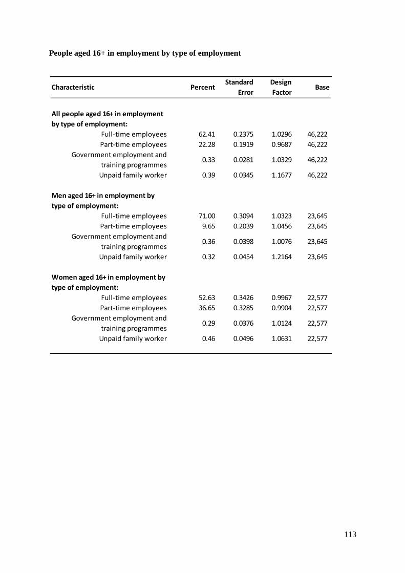
113

People aged 16+ in employment by type of employment

Characteristic PercentStandard

Error

Design

FactorBase

All people aged 16+ in employment

by type of employment:

Full-time employees 62.41 0.2375 1.0296 46,222

Part-time employees 22.28 0.1919 0.9687 46,222

Government employment and

training programmes0.33 0.0281 1.0329 46,222

Unpaid family worker 0.39 0.0345 1.1677 46,222

Men aged 16+ in employment by

type of employment:

Full-time employees 71.00 0.3094 1.0323 23,645

Part-time employees 9.65 0.2039 1.0456 23,645

Government employment and

training programmes0.36 0.0398 1.0076 23,645

Unpaid family worker 0.32 0.0454 1.2164 23,645

Women aged 16+ in employment by

type of employment:

Full-time employees 52.63 0.3426 0.9967 22,577

Part-time employees 36.65 0.3285 0.9904 22,577

Government employment and

training programmes0.29 0.0376 1.0124 22,577

Unpaid family worker 0.46 0.0496 1.0631 22,577

114

People aged 16+ in employment by industry sectors

Characteristic PercentStandard

Error

Design

FactorBase

All people aged 16+ in employment

by industry sector:

Agriculture & Fisheries 1.12 0.0591 1.1786 46,222

Energy & Water 1.83 0.0663 1.0392 46,222

Manufacturing 9.69 0.1494 1.0605 46,222

Construction 7.30 0.1318 1.0638 46,222

Distribution 18.30 0.1994 1.0828 46,222

Transport and Communication 8.96 0.1483 1.0903 46,222

Banking, Finance & Insurance 16.45 0.1914 1.0842 46,222

Public Admin, Health & Education 29.92 0.2245 1.0298 46,222

Other Services 5.80 0.1210 1.0873 46,222

Men aged 16+ in employment by

industry sector:

Agriculture & Fisheries 1.62 0.0899 1.0785 23,645

Energy & Water 2.69 0.1084 1.0145 23,645

Manufacturing 13.73 0.2319 1.0202 23,645

Construction 12.10 0.2249 1.0439 23,645

Distribution 17.53 0.2637 1.0501 23,645

Transport and Communication 12.45 0.2257 1.0350 23,645

Banking, Finance & Insurance 17.19 0.2623 1.0525 23,645

Public Admin, Health & Education 17.01 0.2555 1.0295 23,645

Other Services 5.05 0.1537 1.0627 23,645

Women aged 16+ in employment by

industry sector:

Agriculture & Fisheries 0.56 0.0503 0.9793 22,577

Energy & Water 0.85 0.0632 1.0009 22,577

Manufacturing 5.11 0.1536 1.0137 22,577

Construction 1.84 0.0940 1.0175 22,577

Distribution 19.18 0.2717 1.0025 22,577

Transport and Communication 5.00 0.1570 1.0464 22,577

Banking, Finance & Insurance 15.61 0.2539 1.0160 22,577

Public Admin, Health & Education 44.61 0.3416 0.9983 22,577

Other Services 6.66 0.1779 1.0363 22,577

115

Economically active people 16+ by sex who were ILO unemployed

Characteristic PercentStandard

Error

Design

FactorBase

Economically active people aged 16+

who were ILO unemployed:

All persons 16+ 5.52 0.1142 0.9844 48,765

Men 16+ 5.73 0.1590 1.0666 24,990

Women 16+ 5.27 0.1550 1.0353 23,775

Economically active people aged 16-17

who were ILO unemployed:

All persons 16-17 27.26 1.6483 1.0148 760

Men 16-17 35.33 2.6167 1.0214 348

Women 16-17 20.12 2.0092 1.0072 412

Economically active people aged 18-24

who were ILO unemployed:

All persons 18-24 14.02 0.5165 1.0453 4,916

Men 18-24 15.57 0.7309 1.0113 2,505

Women 18-24 12.30 0.7044 1.0538 2,411

Economically active people aged 25-34

who were ILO unemployed:

All persons 25-34 4.98 0.2377 1.0954 10,041

Men 25-34 5.08 0.3451 1.1069 4,999

Women 25-34 4.87 0.3174 1.0447 5,042

Economically active people aged 35-49

who were ILO unemployed:

All persons 35-49 3.84 0.1555 1.0601 17,147

Men 35-49 3.50 0.2074 1.0538 8,734

Women 35-49 4.21 0.2265 1.0329 8,413

Economically active people aged 50-64

who were ILO unemployed:

All persons 50-64 3.49 0.1631 1.0532 13,937

Men 50-64 3.74 0.2288 1.0252 7,199

Women 50-64 3.22 0.2209 1.0317 6,738

Economically active people aged 65+

who were ILO unemployed:

All persons 65+ 1.84 0.3883 1.0951 1,964

Men 65+ 2.15 0.5319 1.1175 1,205

Women 65+ 1.37 0.4947 0.9844 759

116

People aged 16+ in employment by region of usual residence (GOR)

Characteristic PercentStandard

Error

Design

FactorBase

All persons aged 16+ in

employment:

North East 55.18 0.8566 0.9482 3,321

North West 59.06 0.6424 1.0590 6,726

Merseyside 53.38 1.6754 1.3449 1,395

Yorkshire & Humberside 57.78 0.5843 0.9268 6,617

East Midlands 59.19 0.6302 0.9338 5,523

West Midlands 57.56 0.6140 0.9999 6,013

Eastern 61.74 0.5548 0.9444 7,135

London 63.40 0.5441 1.1076 7,919

South East 62.77 0.4688 0.9731 10,191

South West 60.42 0.6141 0.9932 6,345

Wales 54.67 0.8556 1.0277 3,592

Scotland 59.83 0.6175 0.9941 6,224

Northern Ireland 57.58 0.9628 0.8828 2,767

All persons aged 16+ ILO

unemployed:

North East 4.56 0.3711 0.9795 3,321

North West 3.32 0.2317 1.0486 6,726

Merseyside 4.16 0.6362 1.2752 1,395

Yorkshire & Humberside 3.96 0.2536 1.0193 6,617

East Midlands 3.09 0.2425 1.0204 5,523

West Midlands 3.93 0.2660 1.1021 6,013

Eastern 2.81 0.1991 0.9969 7,135

London 4.16 0.2493 1.2249 7,919

South East 2.81 0.1703 1.0342 10,191

South West 2.73 0.2255 1.0948 6,345

Wales 3.85 0.3512 1.0917 3,592

Scotland 3.72 0.2609 1.0882 6,224

Northern Ireland 3.77 0.3909 0.9303 2,767

All persons aged 16+

economically inactive:

North East 40.26 0.8279 0.9293 3,321

North West 37.63 0.6296 1.0535 6,726

Merseyside 42.46 1.6709 1.3537 1,395

Yorkshire & Humberside 38.26 0.5606 0.9036 6,617

East Midlands 37.72 0.6013 0.9035 5,523

West Midlands 38.51 0.5861 0.9694 6,013

Eastern 35.45 0.5388 0.9319 7,135

London 32.44 0.5260 1.1017 7,919

South East 34.42 0.4564 0.9639 10,191

South West 36.85 0.6032 0.9891 6,345

Wales 41.48 0.8461 1.0269 3,592

Scotland 36.45 0.5907 0.9686 6,224

Northern Ireland 38.66 0.9080 0.8450 2,767

117

People aged 16+ by ethnic origin

Characteristic PercentStandard

Error

Design

FactorBase

White

All persons 16+ 88.73 0.1646 1.4140 73,768

Men 16+ 88.76 0.1991 1.1816 35,154

Women 16+ 88.70 0.1837 1.1405 38,614

Mixed

All persons 16+ 0.94 0.0435 1.2257 73,768

Men 16+ 0.94 0.0588 1.1430 35,154

Women 16+ 0.94 0.0544 1.1092 38,614

Asian or Asian British

All persons 16+ 5.53 0.1330 1.5804 73,768

Men 16+ 5.75 0.1559 1.2557 35,154

Women 16+ 5.32 0.1414 1.2382 38,614

Black or Black British

All persons 16+ 2.61 0.0871 1.4819 73,768

Men 16+ 2.32 0.1000 1.2449 35,154

Women 16+ 2.89 0.1096 1.2847 38,614

Chinese

All persons 16+ 0.50 0.0424 1.6305 73,768

Men 16+ 0.50 0.0622 1.6525 35,154

Women 16+ 0.50 0.0436 1.2110 38,614

Other

All persons 16+ 1.59 0.0711 1.5426 73,768

Men 16+ 1.62 0.0849 1.2595 35,154

Women 16+ 1.57 0.0789 1.2485 38,614