Office for Budget Responsibility Forecast evaluation ...obr.uk/docs/dlm_uploads/Forecast-evaluation-report-October-2016-1.pdf · Printed on paper containing 75% recycled fibre content

Forecast evaluation report

October 2016

Office for Budget ResponsibilityForecast evaluation report

Presented to Parliament pursuant to Section 8 of the Budget Responsibility

and National Audit Act 2011

October 2016

© Crown copyright 2016 This publication is licensed under the terms of the Open Government Licence v3.0 except where otherwise stated. To view this licence, visit nationalarchives.gov.uk/doc/open-government-licence/version/3 or write to the Information Policy Team, The National Archives, Kew, London TW9 4DU, or email: [email protected].

Where we have identified any third party copyright information you will need to obtain permission from the copyright holders concerned.

This publication is available at www.gov.uk/government/publications

Any enquiries regarding this publication should be sent to us at [email protected]

Print ISBN 9781474137591 Web ISBN 9781474137607

ID 28091611 10/16 57096

Printed on paper containing 75% recycled fibre content minimum

Printed in the UK by the Williams Lea Group on behalf of the Controller of Her Majesty’s Stationery Office

Contents

Foreword ................................................................................................................ 1

Chapter 1 Executive Summary .................................................................................................. 3

Chapter 2 The economy .......................................................................................................... 9

Introduction ........................................................................................................ 9

June 2010 economy forecast review .................................................................... 9

The level and growth of GDP ............................................................................. 19

March 2014 and 2015 forecasts in detail ........................................................... 24

The composition of GDP ................................................................................... 25

Developments by sector .................................................................................... 27

The labour market and productivity .................................................................... 35

Potential output ................................................................................................. 37

Chapter 3 The public finances ............................................................................................... 39

Introduction ...................................................................................................... 39

Classification changes ....................................................................................... 39

Public sector net borrowing ............................................................................... 41

June 2010 forecast in detail .............................................................................. 41

March 2014 and 2015 forecasts in detail ........................................................... 48

Chapter 4 Refining our forecasts ............................................................................................ 67

Introduction ...................................................................................................... 67

Lessons to learn ................................................................................................ 67

Review of fiscal forecasting models .................................................................... 68

Annex A Detailed economy and fiscal tables ........................................................................ 79

Annex B Comparison with past official forecasts ................................................................... 99

Index of charts and tables .................................................................................... 107

Foreword

The Office for Budget Responsibility (OBR) was created in 2010 to provide independent and authoritative analysis of the UK public finances. Twice a year – at the time of each Budget and Autumn Statement – we publish a set of forecasts for the economy and the public finances over the coming five years in our Economic and fiscal outlook (EFO). We use these forecasts to assess the Government’s progress against the fiscal targets that it has set itself.

In each EFO, we stress the uncertainty that lies around all such forecasts. We compare our central forecasts to those of other forecasters. We point out the confidence that should be placed in our central forecast given the accuracy of past official forecasts. We use sensitivity and scenario analysis to show how the public finances could be affected by alternative economic outcomes. And we highlight uncertainties in how the public finances will evolve, even if one were to know with confidence how the economy was going to behave – for example, because of uncertain estimates of the cost or yield associated with new policy measures.

Notwithstanding these uncertainties – and the fact that no one should expect any economic or fiscal forecast to be right in its entirety – we believe that it is important to spell out our central forecast in considerable quantitative detail and then to examine and explain after the event how it compares to subsequent outturn data. That is what we endeavour to do in this report.

We believe that it is important to publish the detail of our forecasts for two main reasons:

• the first is transparency and accountability: the whole rationale for contracting out the official fiscal forecast to an independent body is to reassure people that it reflects dispassionate professional judgement rather than politically motivated wishful thinking – even if people disagree with the particular conclusions we have reached. The best way to do that is to ‘show our working’ as clearly as we can; and

• the second is self-discipline: the knowledge that you are going to have to justify your forecast in detail forces you to make only those judgements you are willing to defend. You cannot hide them in the knowledge that no one will ever know.

Assessing the performance of our forecasts after the event is also important for transparency and accountability – and for helping users to understand how they are made and revised. Identifying and explaining forecast errors also helps improve our understanding of the way in which the economy and public finances behave, and hopefully allows us to improve our judgements and forecast techniques for the future. We hope to take that a step further over the coming year as we undertake a systematic review of the forecasting models that are used to help us construct each line of our fiscal forecasts.

1 Forecast evaluation report

Foreword

It is worth noting that when we use the word ‘errors’ in this report we are simply referring to the arithmetic difference between the forecast and the outturn. We are not implying that it would have been possible to avoid them given the information available at the time the forecast was made – differences with outturns may reflect unforeseeable developments after the forecast was made.

In judging our own performance – and in assessing the relative performance of different forecasters – it is also important to remember that the current outturn data represent a relatively early draft of economic history. The stories we have told in previous reports look different after subsequent data revisions. So what appear to have been accurate or inaccurate forecasts today may look very different in the wake of inevitable and often large statistical revisions. This was certainly the experience of the recession and recovery of the 1990s and there continue to be significant revisions to the history of the late 2000s recession and the ongoing recovery.

We have continued the approach used in past reports of trying to understand the underlying stories that have driven our forecast errors. But, as in previous reports and the Treasury’s End of year fiscal reports that preceded them, we also present the detailed decomposition of specific fiscal year forecasts. As with all our reports, we would be very grateful for feedback on its content and for suggestions to improve future reports.

The forecasts we publish represent the collective view of the three independent members of the OBR’s Budget Responsibility Committee (BRC). Our economic forecast is produced entirely by OBR staff working with the BRC. For the fiscal forecast, given its highly disaggregated nature, we also draw heavily on the help and expertise of officials from across Government, most notably in HM Revenue and Customs and the Department for Work and Pensions. We are very grateful for this work and for the analysis that they have contributed to the production of this report. While recognising these valuable contributions, we also stress that the BRC takes full responsibility for the judgements underpinning the forecasts and for the errors presented in this report.

Forecast evaluation report 2

Robert Chote Sir Stephen Nickell Graham Parker CBE

The Budget Responsibility Committee

1 Executive summary

1.1 Forecasts provide an essential basis for setting policy. But since the future can never be known with anything approaching precision, forecasts are surrounded by significant uncertainty and will inevitably prove to be wrong in many respects.

1.2 We stress these uncertainties in every Economic and fiscal outlook (EFO), presenting fan charts around our main forecasts, sensitivity analysis of key assumptions and the fiscal implications of different economic scenarios. And once a year, in our Forecast evaluation report (FER), we compare the latest outturn data for the economy and public finances to our earlier forecasts and try to explain the inevitable differences. (We refer to the arithmetic difference between these forecasts and outturns as ‘errors’, but this does not necessarily mean that they could have been avoided given the information available at the time.)

1.3 The backdrop to this report is:

• a real economy that has been growing at close to historical average rates for the past few years, after a period when it repeatedly disappointed relative to forecast;

• a labour market that has continued to be stronger than expected in employment terms, but weaker in terms of earnings and productivity growth; and

• falls in the budget deficit and a slowing in the pace at which public debt is rising.

1.4 As this report is focused on comparing past forecasts with available outturn data, it should not be affected by any economic and fiscal consequences that follow from the result of the referendum on the UK’s membership of the European Union. We might expect that to become a feature of future FERs.

What questions does this report seek to answer?

1.5 The focus of this year’s report is 2015-16. That was the final year of our first forecast published in June 2010, so we revisit the questions we have asked about that forecast in previous reports. Why did real GDP growth fall short of forecast? Why was nominal GDP growth weaker still? And how did that and other factors explain the much higher-than-expected budget deficit by 2015-16?

1.6 We also carry out our usual detailed analysis of the one- and two-year ahead forecast errors for 2015-16, which this year means looking at our March 2014 and March 2015 forecasts. The questions we ask here are more specific, since the differences between forecast and outturn for headline GDP growth and borrowing are relatively small.


Executive summary

Explaining our forecast errors for 2015-16

June 2010 forecast

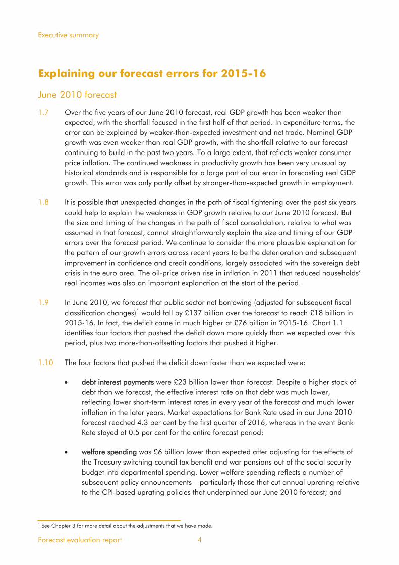
1.7 Over the five years of our June 2010 forecast, real GDP growth has been weaker than expected, with the shortfall focused in the first half of that period. In expenditure terms, the error can be explained by weaker-than-expected investment and net trade. Nominal GDP growth was even weaker than real GDP growth, with the shortfall relative to our forecast continuing to build in the past two years. To a large extent, that reflects weaker consumer price inflation. The continued weakness in productivity growth has been very unusual by historical standards and is responsible for a large part of our error in forecasting real GDP growth. This error was only partly offset by stronger-than-expected growth in employment.

1.8 It is possible that unexpected changes in the path of fiscal tightening over the past six years could help to explain the weakness in GDP growth relative to our June 2010 forecast. But the size and timing of the changes in the path of fiscal consolidation, relative to what was assumed in that forecast, cannot straightforwardly explain the size and timing of our GDP errors over the forecast period. We continue to consider the more plausible explanation for the pattern of our growth errors across recent years to be the deterioration and subsequent improvement in confidence and credit conditions, largely associated with the sovereign debt crisis in the euro area. The oil-price driven rise in inflation in 2011 that reduced households’ real incomes was also an important explanation at the start of the period.

1.9 In June 2010, we forecast that public sector net borrowing (adjusted for subsequent fiscal classification changes) would fall by £137 billion over the forecast to reach £18 billion in 2015-16. In fact, the deficit came in much higher at £76 billion in 2015-16. Chart 1.1 identifies four factors that pushed the deficit down more quickly than we expected over this period, plus two more-than-offsetting factors that pushed it higher.

1.10 The four factors that pushed the deficit down faster than we expected were:

• debt interest payments were £23 billion lower than forecast. Despite a higher stock of debt than we forecast, the effective interest rate on that debt was much lower, reflecting lower short-term interest rates in every year of the forecast and much lower inflation in the later years. Market expectations for Bank Rate used in our June 2010 forecast reached 4.3 per cent by the first quarter of 2016, whereas in the event Bank Rate stayed at 0.5 per cent for the entire forecast period;

• welfare spending was £6 billion lower than expected after adjusting for the effects of the Treasury switching council tax benefit and war pensions out of the social security budget into departmental spending. Lower welfare spending reflects a number of subsequent policy announcements – particularly those that cut annual uprating relative to the CPI-based uprating policies that underpinned our June 2010 forecast; and

1

1 See Chapter 3 for more detail about the adjustments that we have made.


Executive summary

• resource and capital spending by departments (departmental expenditure limits, or RDEL and CDEL) each came in £0.6 billion below forecast, after adjusting for major switches between the categories that the Treasury uses to manage overall spending.

1.11 Two countervailing upward pressures more than offset these factors and left the cash deficit significantly higher overall than we had forecast:

• receipts were £85 billion weaker than expected. The weakness in nominal GDP growth alone would have implied receipts shortfall by 2015-16 of around £70 billion. But they were a further £15 billion below forecast, largely reflecting the fact that the receipts-to-GDP ratio was 0.8 percentage points lower than expected. A much weaker effective tax rate on income tax and NICs explains around £28 billion of that error; and

• there was also a small contribution from other spending being £4 billion higher than expected. After adjusting for significant historical switches between the categories that the Treasury uses to manage overall spending, over half of the underlying error is driven by higher borrowing-financed capital spending by local authorities.

Chart 1.1: June 2010 PSNB forecast error for 2015-16 (in cash terms)

17.6

-6.0 -0.6 -0.6

+3.9

76.5

-22.6

+84.8

-20

0

20

40

60

80

100

June 2010forecast

Debt interest Welfare RDEL CDEL Other spending Receipts Outturn

£ bi

llion

Errors adding to net borrowing

Errors subtracting from net borrowing

Source: ONS, OBRNote: Our June 2010 forecast has been restated for major classification and methodological changes.

1.12 The fall in the deficit was also smaller than we expected as a share of GDP. Rather than

dropping from 11.0 per cent in 2009-10 to 0.9 per cent in 2015-16, the latest outturns show a decline from 10.1 to 4.1 per cent. The unexpected weakness of nominal GDP growth over this period means that all the factors listed above (bar lower debt interest spending) helped keep the deficit higher than we expected. For example, although welfare spending came in £6.0 billion lower than forecast in cash terms, it came in 0.7 percentage

2

2 As set out in Chapter 3, the analysis of errors as a share of GDP presented here has been adjusted to abstract from the effect of the large upward revisions to the level of nominal GDP since our June 2010 forecast. See Chapter 3 for more detail.


Executive summary

points higher than we forecast as a share of GDP. This reflects the fact that average benefit and tax credit awards did not fall as fast as we expected relative to average incomes.

March 2014 and March 2015 forecasts

1.13 Our forecast for real GDP growth changed little between March 2014 and March 2015. Our March 2014 forecast underestimated the extent to which real GDP growth would be driven by private consumption. Both forecasts overestimated the extent to which growth would be supported by private investment and underestimated the contribution of government spending. These compositional errors were slightly greater in March 2014 than in March 2015. Nominal GDP growth was slightly weaker than either forecast predicted, with weakness in nominal private investment and consumer spending growth the biggest factors (particularly relative to our March 2014 forecast).

1.14 In terms of public sector net borrowing in 2015-16:

• our March 2014 forecast was too optimistic: net borrowing was around £5 billion higher than forecast. That difference is more than explained by weak tax receipts, partly offset by lower spending. Weaker receipts were partly driven by tax base effects (with lower average earnings reducing income tax and NICs receipts and a lower oil price hitting North Sea oil revenues) and partly by effective tax rate effects (particularly by weakness at the ‘tax-rich’ top end of the residential property market). The partial offset from lower spending is more than explained by lower debt interest spending, where both inflation and interest rates were much lower-than-expected; and

• our March 2015 forecast was too pessimistic: net borrowing was around £3 billion lower than forecast. Strength in the main receipts lines was partly offset by local authorities drawing down on their reserves by more than expected to boost spending.

Refining our forecasts

Lessons to learn

1.15 It is often the case that the lessons emerging from our FERs have already been acted upon because they were identified during an EFO forecast process. In some areas, that has been repeated this year. Lessons that have been reinforced include:

• the importance of the composition of labour income, noting that employment-driven growth has been less tax-rich than earnings-driven growth would have been;

• savings associated with major reforms of the incapacity and disability benefits systems had fallen short of expectations, due largely to challenges in delivering the reforms;

• the behaviour of local authorities in response to tighter financial settlements. In particular, the addition to and use of reserves has been a source of error in our previous forecasts and has again appeared as an issue in this year’s analysis; and


Executive summary

• in our last FER we identified a persistent source of over-pessimism in the VAT forecast. This was corrected in our November 2015 forecast, so is a factor in explaining the errors in our March 2014 and March 2015 forecasts.

1.16 There are also new issues and themes that have been identified in this year’s evaluation. These include:

• the effect of rising tax-motivated incorporations on our receipts forecast. Flows from employment to incorporation reduce receipts from income tax and NICs and increase corporation tax receipts by a less-than-offsetting amount. We appear to have under-estimated this effect, although there are no outturn data against which to compare our forecasts. We plan to adopt a new model to underpin our next forecast. At this stage it is not clear how large the effect on receipts will be, although it will be negative overall;

• the difficulty in forecasting stamp duty land tax receipts during a period of substantial and regionally varied house price movements, and significant – often pre-announced – policy changes that have generated large behavioural responses from taxpayers; and

• the challenges in forecasting self-assessment income tax receipts. The forecast relies on inputs that are not necessarily closely aligned with the true tax base, which creates uncertainty about the assumptions that need to be fed into the forecasting model. The self-assessment forecast has also had to factor in the effects of a large number of anti-avoidance measures that are particularly difficult to estimate. We evaluated some of these measures in Working paper No.8: Anti-avoidance costings: an evaluation.

Review of fiscal forecasting models

1.17 In this year’s FER we set out our plan for a first systematic review of the fiscal forecasting models that are used in the preparation of our forecasts, based on the analysis of forecast errors in this and previous FERs.

1.18 We use a large number of fiscal forecasting models – varying greatly in size and sophistication – to generate our bottom-up forecasts of tax and spending. These models are typically owned and maintained by other parts of government that are responsible for administering the element of the public finances being forecast. It is important to understand that it is not the forecast model that determines the shape of the forecast it produces; it is the assumptions and judgements that are fed into it by the forecaster. For our forecasts, while the models are typically operated outside the OBR, the assumptions and judgements that are fed into them are determined by the Budget Responsibility Committee.

1.19 Given the large number of models in use, we plan to focus the review on those models that are used to forecast the biggest elements of tax and non-departmental spending and those that have on average exhibited larger errors (once the effects of economy forecast errors, classification changes and subsequent policy announcements have been accounted for – termed ‘fiscal forecasting’ errors in our reports).


Executive summary

1.20 It is important to recognise that while issues with the model used to produce a forecast could explain some of the fiscal forecasting error, the model itself is unlikely to be the only source of that error. Indeed, even though we have excluded economy, policy and classification effects that do not relate to the model, it is still probably more likely that the error will relate to how the model was used rather than something inherent to the model itself. That means that we need to be careful when interpreting the analysis of forecast accuracy that follows, because it will capture a wide range of factors that fall into two main categories:

• factors directly related to the model, such as the specification of the tax system in a microsimulation model or the coefficients used in an econometric equation; or

• judgements that are fed into the model, which could include assumptions about changes in the earnings distribution (which we factor into our income tax and NICs forecast, but do not forecast specifically), the economic determinant chosen as a proxy for a tax or spending base (such as the FTSE All-share index used to proxy equity disposals in the CGT forecast) and other judgements (such as the eligibility and take-up of a social security benefit). These judgements can often reflect events that are highly uncertain, such as the outcome of a litigation case or the emergence of new non-compliance behaviour.

1.21 We need to learn from both sources of forecast error, but in order to take the appropriate remedial action we need to know the true cause. The unexpected loss of a legal challenge might generate a big fiscal forecasting error, but it would not necessarily indicate a modelling issue that needed to be addressed.

Comparison with past official forecasts

1.22 We also compare the size of our forecast errors against past official forecast errors (in Annex B). The exercise has obvious limitations as a guide to relative forecast performance. Most fundamentally, we are not comparing like with like given the many factors that can affect the public finances and that vary significantly over time. And, as the OBR has only produced 14 forecasts so far, the sample is still relatively small. This is particularly true at longer time horizons – we can compare only five of our forecasts at a 4-year horizon and just three at a 5-year horizon. For what it is worth, given the limitations of such comparisons, the errors in our real GDP and borrowing forecasts have, more often than not, been smaller than the average errors in official forecasts over the past 20 years.


2 The economy

Introduction

2.1 The focus of this year’s Forecast evaluation report (FER) is the performance of three of our previous forecasts for the 2015-16 fiscal year. In this chapter:

• we start by considering our June 2010 forecast in isolation, given that initial outturn data are now available for the full period of that forecast. We compare it against the very different path that the economy took over the past five years, drawing on analysis presented in previous FERs (from paragraph 2.2). We look again at whether changes in the path of fiscal consolidation or errors in our assumptions about its effect on the economy might explain the big differences between our forecast and latest outturns (from paragraph 2.11). We explain how real and nominal GDP growth have evolved relative to our forecasts since June 2010 (from paragraph 2.18); and

• we then look at our March 2014 and March 2015 forecasts. We show first how monetary policy has differed from market expectations at the time of our forecasts (from paragraph 2.27) and how other market-derived assumptions (from paragraph 2.28) have evolved. We then assesses developments in the composition of GDP (from paragraph 2.29) and individual sectors of the economy (from paragraph 2.33). Lastly, we consider the behaviour of the labour market and therefore productivity (from paragraph 2.50) and potential output (from paragraph 2.55).

June 2010 economy forecast review

2.2 Now that outturn data are available for the duration of the June 2010 forecast period, it is possible to compare the entirety of that forecast with the latest economy data.

Headline GDP and its components

2.3 Real GDP growth has been weaker than our June 2010 forecast, but the shortfall in nominal GDP growth has been larger, especially after the latest revisions to ONS data. Up to the end of 2012, real GDP growth was lower than we forecast, which was also reflected in lower than expected nominal GDP. From 2013 onwards, real GDP growth has been close to our June 2010 forecast, albeit from a lower starting point. During this latter period, whole economy inflation has been lower than expected, which has further reduced nominal GDP relative to our forecast. This is significant for the public finances, because tax receipts are heavily influenced by nominal GDP, as is the share of GDP devoted to public spending.


The economy

Chart 2.1: Cumulative errors in June 2010 GDP forecasts since 2010Q1

-14

-12

-10

-8

-6

-4

-2

0

2

Q12010

Q3 Q12011

Q3 Q12012

Q3 Q12013

Q3 Q12014

Q3 Q12015

Q3 Q12016

Perc

enta

ge p

oint

s

Real GDP Nominal GDP

Source: ONS, OBR


2.4 In terms of the expenditure components of GDP, private consumption growth has been close to our June 2010 forecast, but investment has been weaker than we expected and net trade has been a drag on growth, having been expected to make a positive contribution. These two errors more than explain our GDP forecast error. They are partly offset by government consumption, which was stronger than expected.

The economy

Chart 2.2: Contributions to real GDP growth since 2010Q1

-25

-20

-15

-10

-5

0

5

10

15

20

25

30

35

40

June 2010 Latest Difference

Perc

enta

ge p

oint

s

Private consumption Total investment Government consumption

Net trade Stocks Valuables

Total

Source: OBR calculations 2.5 While our forecast for real consumption growth was close to the latest outturn data, the

private consumption deflator has been weaker than we expected. The resulting shortfall in nominal private consumption growth explains around a third of our forecast error for nominal GDP. Investment growth has also been weaker than expected, with the error in that case related to its contribution to growth in real GDP rather than the deflator. The same has been true of net trade.

Chart 2.3: Contributions to nominal GDP growth since 2010Q1

-25

-20

-15

-10

-5

0

5

10

15

20

25

30

35

40


Perc

enta

ge p

oint

s

Private consumption Total investment

Government consumption Net trade

Stocks Valuables

Total

Source: OBR calculations


The economy

2.6 The continued weakness in productivity growth has been very unusual by historical standards and as a result productivity growth has fallen well short of our June 2010 forecast. As Chart 2.4 shows, this was responsible for a large part of our error in forecasting real GDP growth. Employment growth has been higher than we forecast in June 2010, due to lower than expected unemployment and higher than expected participation, but in terms of GDP growth this was not enough to offset weaker-than-expected productivity growth.

1

Chart 2.4: Contributions to real GDP growth from labour inputs and productivity since 2010Q1

-15

-10

-5

0

5

10

15

20


Perc

enta

ge p

oint

s

Productivity Average hours Population

Participation Real GDP


2.7 CPI inflation was forecast to return close to the Bank of England’s 2 per cent target by the start of 2012, remaining close to target for the rest of the forecast period. In fact CPI inflation was significantly higher than forecast up to 2013, but has since fallen well below the Bank’s target. Large fluctuations in oil prices were one source of those errors.

2.8 House price inflation was forecast to pick up slowly over 2011 and 2012, before settling at around 5 per cent a year. In fact, the middle of 2010 turned out to be a local peak for house prices, not surpassed again until mid-2013. House price inflation picked up after that, but house price growth was 1.6 percentage points lower than our June 2010 forecast up to the start of 2016.

2.9 World GDP growth has been somewhat weaker than we expected, but world trade growth has been much weaker. That implies a lower trade intensity of global output, so that even accounting for the lower GDP growth, trade growth has been lower than we would have expected. That has fed through to lower-than-expected growth in UK export markets,

1 For an overview of the ‘productivity puzzle’ and some of the possible explanations of its size and persistence, see The UK productivity puzzle, Bank of England quarterly bulletin, June 2014.


The economy

although the error in our forecast for UK export markets is slightly smaller. This is because the shortfall in world trade growth compared with our June 2010 forecast has been disproportionately due to lower trade in economies that have a lower weight in UK export markets.

Chart 2.5: Growth of world economy variables since 2010Q1

0

5

10

15

20

25

30

35

40

45

50

World GDP World trade UK export markets

Per c

ent

June 2010

Latest

Source: IMF, OECD, OBR calculations

2.10 UK exports have fallen short of our forecast by more than would be explained by the weakness of export markets growth, implying a weaker-than-expected path for the UK’s export market share. We also expected the price of exports to rise, but instead they have remained almost unchanged. This weakness in export prices has also reduced the growth in nominal exports since the first quarter of 2010.


The economy

Chart 2.6: Contributions to nominal exports growth since 2010Q1

-30

-20

-10

0

10

20

30

40

50

60


Perc

enta

ge p

oint

s

Export prices UK export markets

UK export market share Nominal exports


Fiscal policy and growth since 2010

2.11 Over the past six years there has been a large discretionary fiscal tightening in the UK. Chart 2.7 shows the discretionary tightening or loosening in each fiscal year, relative to a Budget 2008 baseline, based on the definition used by the Institute for Fiscal Studies (IFS). The chart shows the plans for fiscal consolidation as set out in the June 2010 Budget, together with the IFS’s estimates produced after the March 2016 Budget.

2.12 The IFS’s March 2016 estimates of the fiscal consolidation up to 2015-16 are broadly unchanged from those set out in our 2015 FER. They suggest that the degree of fiscal tightening between 2009-10 and 2010-11 was slightly smaller than originally planned, while the additional tightening in 2011-12 was larger than expected, as departments underspent relative to plans. The degree of tightening was slightly smaller than expected over the period 2012-13 to 2015-16 as a whole. These revisions are small relative to the cumulative fiscal tightening across the period.


The economy

Chart 2.7: Fiscal consolidation relative to Budget 2008 baseline

-2

0

2

4

6

8

10

12

2008-09 2009-10 2010-11 2011-12 2012-13 2013-14 2014-15 2015-16 2016-17 2017-18 2018-19 2019-20 2020-21

Per c

ent o

f GD

P

June 2010 March 2016

Source: IFS

Chart 2.8: Additional fiscal tightening or loosening each year

-1.0

-0.5

0.0

0.5

1.0

1.5

2.0

2.5

3.0

2008-09 2009-10 2010-11 2011-12 2012-13 2013-14 2014-15 2015-16 2016-17 2017-18 2018-19 2019-20 2020-21

Per c

ent o

f GD

P


Source: IFS

2.13 We use estimates of fiscal multipliers, which unwind over time, to calculate the likely effect of changes to discretionary fiscal policy on growth. These imply that a discretionary tightening of 1 per cent of GDP would reduce output by between 1 per cent (in the case of cuts to capital spending) and 0.3 per cent (for income tax and NICs increases) in the first instance, with the impact unwinding over time such that ultimately fiscal consolidation does not reduce long-term potential output. Chart 2.9 shows the impact of discretionary fiscal policy on GDP growth in each year between 2008-09 and 2015-16 on the basis of IFS


The economy

consolidation estimates at the time of successive forecasts. With little revision to the IFS’s estimates of the consolidation over the past six years, the implied effect of the consolidation on GDP over this period remains broadly unchanged from the estimates we published last year – and suggest that the fiscal consolidation may have reduced the level of real GDP in 2015-16 by around 1.2 per cent. The estimated effect on growth in 2015-16 is zero, as the -0.5 percentage point effect of new consolidation in the year was offset by the +0.5 percentage point effect of previous years’ consolidation effects unwinding.

2

Chart 2.9: Implied impacts of discretionary fiscal policy on GDP growth

-1.5

-1.2

-0.9

-0.6

-0.3

0.0

0.3

0.6

2008-09 2009-10 2010-11 2011-12 2012-13 2013-14 2014-15 2015-16

Per c

ent o

f GD

P

June 2010

July 2015

March 2016

Source: OBR

2.14 It remains possible that the larger-than-expected fiscal tightening in 2011-12 could help to explain the weakness of GDP growth in this period relative to our June 2010 forecast. It is also possible that the unexpected strength of growth in 2014 can partly be explained by the smaller than expected tightening in 2014-15. But the size and timing of the changes in the path of fiscal consolidation cannot straightforwardly explain the scale and timing of our errors over the forecast period. We continue to consider the more plausible explanation for the pattern of our growth errors across recent years to be the deterioration and subsequent improvement in confidence and credit conditions, largely associated with the sovereign debt crisis in the euro area. The oil-price driven rise in inflation in 2011 that reduced households’ real incomes was also an important explanation at the start of the period.

2.15 An alternative way to consider the fiscal policy stance is by assessing changes in the estimated structural deficit from one year to the next. One drawback of these measures is that they depend heavily on estimates of the cyclical position of the economy – and therefore on estimates of the economy’s underlying potential. Revisions to estimates of potential output can therefore bring about large changes in the apparent path of fiscal

2 See FER 2015 supplementary release – Implied impacts of discretionary fiscal policy on GDP growth (2008-09 to 2014-15), October 2015.


The economy

consolidation, even in the absence of discretionary policy measures. The structural deficit will also be affected by underlying changes to taxes and spending that are not directly related to policy (e.g. the downward trend in North Sea oil production has led to lower oil and gas receipts, which would be treated as a fiscal loosening under this methodology).

2.16 In June 2010, we forecast that the structural current budget would be in surplus by 2015-16, while our latest estimates point to a structural deficit of just under 2 per cent of GDP. But as Chart 2.7 shows, little of this difference results from changes in the path of discretionary fiscal policy decisions. Rather, our revisions to potential output now imply a much smaller improvement in the structural deficit, and errors in forecasting effective tax rates have led to smaller improvements in the structural deficit across a number of years, (Table 3.16). We do not therefore think this approach provides convincing evidence that changes in the pace of fiscal tightening have been the most important explanation of the errors in our real GDP forecasts. And, given the factors set out here, we consider this approach to be less useful than the IFS methodology over the 2010-2015 period.

Detailed comparison of June 2010 forecast and outturns

2.17 Table 2.1 summarises the cumulative growth of key elements of our economy forecast over the June 2010 forecast period and compares them with the latest outturn data. These developments have been analysed in detail in past FERs.


The economy

Table 2.1: Growth in key economy variables from 2010Q1 to 2016Q1

June 2010 forecast Latest data Difference1

UK economyGross domestic product (GDP) 17.2 12.9 -4.3Nominal GDP 35.2 22.9 -12.4Expenditure components of GDP Domestic demand 12.7 14.8 2.0

Household consumption2 11.7 10.6 -1.1General government consumption -10.5 7.7 18.3Fixed investment 47.1 21.8 -25.3

Business 67.6 25.5 -42.1

General government3 -32.0 -18.0 14.0

Private dwellings3 56.7 49.7 -7.0Exports of goods and services 39.8 22.0 -17.7Imports of goods and services 21.7 22.4 0.7Balance of payments current accountPer cent of GDP 1.1 -3.1 -4.3InflationCPI 13.1 13.2 0.0RPI 21.5 18.6 -3.0GDP deflator at market prices 15.4 8.8 -6.6Labour marketEmployment 4.9 8.8 4.0Productivity per hour 12.8 2.5 -10.2Wages and salaries 28.1 18.6 -9.5

Average earnings4 22.2 10.5 -11.6LFS unemployment -26.0 -33.0 -7.1Claimant count -32.5 -53.0 -20.5Household sectorReal household disposable income 11.0 6.8 -4.2House prices 24.1 22.5 -1.6World economy

World GDP at purchasing power parity5 24.5 18.9 -5.6

Euro area GDP5 10.1 3.0 -7.1

World trade in goods and services5 40.8 20.8 -20.0

UK export markets6 41.3 29.4 -11.91 Percentage points, except for the current account, which is given as a per cent of GDP.

Per cent, unless otherwise stated

6 Other countries' imports of goods and services weighted according to the importance of those countries in the UK's total exports.

2 Includes households and non-profit institutions serving households.3 Includes transfer costs of non-produced assets.4 Wages and salaries divided by employees.5 Published on an annual basis, so growth rates are from 2010 to 2015.


The economy

The level and growth of GDP

Real GDP

2.18 Despite eight years having passed since the worst phase of the financial crisis was triggered in September 2008, the performance of the UK economy, and therefore of our forecasts, is still being affected by the shadow of that crisis and the deep recession that it caused.

2.19 The latest data from the Office for National Statistics (ONS) suggest that real GDP fell by 6.1 per cent from its peak in the first quarter of 2008 to its trough in the middle of 2009. Since then, GDP has increased by a cumulative 14.9 per cent over the subsequent seven years. But at an annualised rate of around 2 per cent – and with year-on-year growth topping 3 per cent in only three quarters – there has not been a period of significantly above-average growth during that time, as you would expect during a post-recession recovery. Consequently the level of GDP remains well below the level that would have been recorded had activity made up sufficient lost ground to return to its pre-crisis trend.

2.20 As Charts 2.10 and 2.11 illustrate, our forecasts have evolved not merely to reflect new information and judgements regarding the future, but also to take account of the rewriting of past history by the ONS. Net upward revisions to the estimated level of GDP have reduced the depth of the recession and have made the recovery look stronger.

2.21 The most significant methodological changes in Blue Book 2016 affected the measurement of prices in a way that pushed up nominal GDP (rather than changing the split of a given nominal GDP estimate between real activity and prices, as is often the case). Blue Book 2016 therefore contained smaller revisions to real GDP since 2008 than in previous years. The revisions to nominal GDP are discussed next.


The economy

Chart 2.10: Forecasts and outturns for real GDP from 2008Q1

92

96

100

104

108

112

Q12008

Q12009

Q12010

Q12011

Q12012

Q12013

Q12014

Q12015

Q12016

2008

Q1

= 1

00

June 2010 March 2011 March 2012 March 2013

March 2014 March 2015 March 2016 Latest

Source: ONS, OBRNote: Solid lines represent the outturn data that underpinned the forecasts at the time (the dashed lines).

Chart 2.11: Forecasts and outturns for real GDP growth

-8

-6

-4

-2

0

2

4

Q12009

Q3 Q12010

Q3 Q12011

Q3 Q12012

Q3 Q12013

Q3 Q12014

Q3 Q12015

Q3 Q12016

Perc

enta

ge c

hang

e on

a y

ear e

arlie

r



Source: ONS, OBR

2.22 One feature of the revisions is that the ONS now thinks that the recession started earlier – with output beginning to fall around the time that oil prices peaked at close to $150 a barrel in the spring of 2008 rather than after the Lehman Brothers collapse in September. As Chart 2.12 shows, initial estimates suggested that output was roughly flat in the second quarter of 2008 and fell by a relatively small amount in the third quarter. At its worst, in the


The economy

estimates published during 2012, real GDP was estimated to have fallen by a cumulative 3.2 per cent in those two quarters. The latest estimate shows a 2.3 per cent fall.

2.23 One thing this illustrates is the challenge faced by the ONS when trying to estimate changes in real GDP growth at turning points in the economic cycle. That may be relevant in the coming months when considering how much confidence to place in the ONS’s initial estimates of UK economic activity following the EU referendum.

Chart 2.12: Successive estimates of GDP growth in 2008Q2 and 2008Q3

-2.5

-2.0

-1.5

-1.0

-0.5

0.0

0.5

2009 2010 2011 2012 2013 2014 2015 2016

Per c

ent

2008Q2 2008Q3

Source: ONS

Nominal GDP

2.24 Public discussion of economic forecasts tends to focus on real GDP – the volume of goods and services produced in the economy. But the nominal or cash value is more important for the behaviour of the public finances. Tax receipts are driven more by nominal GDP and so is the share of GDP devoted to public spending, when a large proportion of that spending is set out in multi-year cash plans (public services, grants and administration) or linked to consumer price inflation (benefits and tax credits). The importance of nominal GDP revisions in explaining our fiscal forecast revisions over the past six years was illustrated in Annex B of our March 2016 Economic and fiscal outlook (EFO).

2.25 The ONS revised up the level of nominal GDP in its latest Blue Book, largely due to a methodological change applying to the estimation of imputed rents. The upward revisions were smaller in recent years, where that change had already been applied, but were more significant in years before 2010.


The economy

Chart 2.13: Nominal GDP revisions in Blue Book 2016

2.0

2.5

3.0

3.5

4.0

4.5

5.0

2000 2001 2002 2003 2004 2005 2006 2007 2008 2009 2010 2011 2012 2013 2014 2015 2016

£ tr

illio

n

Before Blue Book 2016 revisions

After Blue Book 2016 revisions

Source: ONS, OBR

2.26 The profile of the revisions to nominal GDP shown in Chart 2.13 meant that the average growth rate between 2000 and 2015 was revised down from 4.1 to 3.7 per cent a year. Indeed, Chart 2.14 shows that following these revisions, cumulative nominal GDP growth since its pre-crisis peak is now estimated to have been almost as weak as our most pessimistic forecast from March 2013 – in marked contrast to the pattern of revisions to real GDP shown in Chart 2.10. But with the main source of this revision being an imputed element of nominal GDP, which is not taxed, it should have little bearing on our fiscal forecasts.


The economy

Chart 2.14: Forecasts and outturns for nominal GDP from 2008Q1

90

100

110

120

130

140

Q12008

Q3 Q12009

Q3 Q12010

Q3 Q12011

Q3 Q12012

Q3 Q12013

Q3 Q12014

Q3 Q12015

Q3 Q12016

2008

Q1

= 1

00



Source: ONS, OBR

Chart 2.15: Forecasts and outturns for nominal GDP growth

-8

-4

0

4

8

Q12009

Q3 Q12010

Q3 Q12011

Q3 Q12012

Q3 Q12013

Q3 Q12014

Q3 Q12015

Q3 Q12016

Perc

enta

ge c

hang

e on

a y

ear e

arlie

r



Source: ONS, OBR


The economy

March 2014 and March 2015 forecasts in detail

Forecast conditioning assumptions

Monetary policy

2.27 The Bank Rate assumptions underpinning our forecasts are based on market expectations at the time of each forecast, derived from the price of interest rate swaps. At the time of our March 2014 forecast, these implied that Bank Rate would rise after a year and increase steadily thereafter, up to around 1.6 per cent by mid-2016. Following the pattern seen repeatedly since the financial crisis, these expectations were pushed back – this time as inflation fell sharply. By March 2015 markets were not anticipating a rate rise until the end of 2015, although that still proved to be too early, as Bank Rate was held unchanged at 0.5 per cent until mid-2016. In August 2016, the Bank of England cut Bank Rate to 0.25 per cent, and markets are currently pricing in the possibility of further cuts in the near future.

Chart 2.16: Successive market expectations for Bank Rate

0

1

2

3

4

5

6

Q12008

Q3 Q12009

Q3 Q12010

Q3 Q12011

Q3 Q12012

Q3 Q12013

Q3 Q12014

Q3 Q12015

Q3 Q12016

Q3 Q12017

Per c

ent



Source: Bank of England, OBR

Other conditioning assumptions

2.28 Our economic forecasts are conditioned on a number of other market-derived assumptions, including oil, equity and government bond prices. These are important fiscal determinants. Table 2.2 compares our March 2014 and March 2015 assumptions to subsequent outturns for the second quarter of 2016:

• having been relatively stable at above $100 a barrel for over three years, the oil price fell sharply in the second half of 2014. Our March 2014 and March 2015 forecasts


The economy

both overestimated the oil price, although the difference between forecast and outturn more than halved by the March 2015 forecast;

• gilt yields have fallen to all-time lows, reflecting expectations of future monetary policy and the safe haven status of UK government bonds. Low yields are also consistent with weaker expectations of future UK growth prospects. Our market-derived assumptions for the weighted average conventional gilt rate have therefore often been too high, despite significant and successive downward revisions;

• the sterling effective exchange rate index (ERI) steadily appreciated over recent years, in part because, despite being weak by historical standards, the UK’s recovery has been stronger than some other major developed economies, particularly in the euro area. More recently, the exchange rate has fallen in each quarter since late 2015 as the economy slowed and uncertainty about the result of the EU referendum increased. Our March 2014 assumption proved identical to the outturn in the most recent quarter (although the path it took from the start of 2014 to mid-2016 was different). Our March 2015 assumption was too high, reflecting the unexpected depreciation up to mid-2016. Sterling has since depreciated significantly, with the ERI averaging 78.6 in September 2016, down 8 per cent on the Q2 average shown in Table 2.2; and

• our March 2014 and March 2015 assumptions for equity price changes were more than 10 percentage points too high in both cases.

Table 2.2: Other conditioning assumptions for 2016Q2

Oil price($ per barrel)

Equity prices(FTSE All-share)

Gilt rate(per cent)

ERI exchange rate (index)

March 2014 forecast 99.3 4005 3.5 85.4March 2015 forecast 68.8 3885 2.2 90.82016Q2 average 46.0 3515 2.4 85.4

Difference1

March 2014 -53.3 -489.9 -1.1 0.0March 2015 -22.9 -369.9 0.3 -5.3

1 Difference in unrounded numbers.

The composition of GDP

2.29 The composition of nominal GDP is as important for the public finances as its overall level, since the effective tax rates on the different components of income and spending vary widely. So to assess our budget deficit forecast errors, it is helpful to examine how the different components of GDP have evolved over time.

The expenditure composition of GDP

2.30 Our forecast for real GDP growth changed little between March 2014 and March 2015. Table 2.3 shows that both forecasts were close to the latest outturn data. Our March 2014 forecast underestimated the extent to which real GDP growth would be driven by private


The economy

consumption. Both forecasts overestimated the extent to which growth would be supported by private investment and underestimated the contribution of government spending. These compositional errors were slightly greater in March 2014 than in March 2015. Nominal GDP growth was slightly weaker than either forecast predicted, with weakness in nominal private investment and consumer spending growth the biggest factors (particularly relative to our March 2014 forecast). The individual elements of these forecasts are discussed later in the chapter.

Table 2.3: Contributions to real GDP growth from 2013Q4 to 2016Q2

Private consumption

Business investment

Residential investment

Total government

Net tradeStocks and

statistical discrepancy

GDP

March 2014 forecast 3.6 1.8 1.1 -0.2 0.1 -0.2 6.3March 2015 forecast 4.2 1.6 0.5 0.6 -0.2 -0.3 6.4Latest data 4.2 0.4 0.6 1.0 -0.3 0.4 6.4

Difference1

March 2014 0.6 -1.4 -0.5 1.1 -0.4 0.7 0.1March 2015 0.0 -1.1 0.1 0.4 0.0 0.8 0.0

Percentage points


Table 2.4: Contributions to nominal GDP growth from 2013Q4 to 2016Q2

Private consumption

Private investment

Total government

Net tradeStocks and


GDP

March 2014 forecast 7.6 3.4 -0.2 0.2 -0.2 10.8March 2015 forecast 6.3 2.9 0.2 0.2 0.7 10.2Latest data 5.7 1.5 0.8 0.5 1.2 9.7

Difference1

March 2014 -1.8 -1.9 1.0 0.3 1.4 -1.1March 2015 -0.6 -1.4 0.6 0.3 0.5 -0.5

Percentage points


Table 2.5: Growth in National Accounts deflators from 2013Q4 to 2016Q2

Private consumption

Private investment

Total government

Exports Imports GDP

March 2014 forecast 5.5 3.6 -0.1 0.2 0.0 4.3March 2015 forecast 3.0 4.7 -1.9 -7.2 -7.7 3.6Latest data 2.2 3.0 -0.8 -4.5 -6.3 3.1

Difference1

March 2014 -3.4 -0.6 -0.6 -4.7 -6.3 -1.1March 2015 -0.8 -1.7 1.1 2.7 1.4 -0.5

Per cent



The economy

The income composition of nominal GDP

2.31 In addition to breaking down changes in GDP between different categories of expenditure, we can also break them down between different categories of income. This is even more important for the public finances, given the amount of revenue raised from taxes on labour income and profits. As with expenditure, the composition of nominal income matters because different components face different effective tax rates. Later in this chapter we also look at the composition of labour income, which has further implications for the tax take.

2.32 Our March 2014 and March 2015 forecasts for compensation of employees both represented significant downward revisions compared with previous forecasts, but even so still proved optimistic due to continued weaker-than-expected average earnings growth. We also revised down our profits forecast in March 2014 and again in March 2015. Latest data show that profits were slightly higher than we expected.

Table 2.6: Contributions to GDP income growth from 2013Q4 to 2016Q2

Compensation of employees

Corporations' gross operating

surplus

Other income

Taxes on products and

productionGDP

Statistical discrepancy

March 2014 forecast 5.7 1.9 2.0 1.2 10.8 0.0March 2015 forecast 5.3 1.5 2.5 0.7 10.1 0.2Latest data 4.1 2.3 2.6 1.0 9.7 -0.2

Difference1

March 2014 -1.6 0.4 0.5 -0.2 -1.1 -0.2March 2015 -1.2 0.8 0.1 0.3 -0.4 -0.4

Percentage points


Developments by sector

Households

2.33 In March 2014 and March 2015, we forecast that disposable income and labour income would grow by around 10 per cent between the end of 2013 and the second quarter of 2016. Latest data show that disposable income grew by just under 10 per cent over that period, but a more narrow measure of labour income grew by 11 per cent.3

2.34 In March 2015, we revised up our forecast for real consumption growth and this has proved to be broadly in line with the latest data. That was consistent with an upward revision to our forecast for real disposable income, which in turn reflected a lower forecast for inflation.

3 Here we define labour income as wages and salaries plus mixed income less households’ social contributions.


The economy

Table 2.7: Income and consumption growth from 2013Q4 to 2016Q2

Nominal disposable

income

Labour income

Nominal consumption

Increase in price

level

Real disposable

income

Real consumption

Saving ratio (change, per

cent)

Adjusted saving ratio1

March 2014 forecast 10.0 10.5 11.4 5.5 4.3 5.6 -0.8 -1.2March 2015 forecast 10.5 10.9 9.7 3.0 7.3 6.5 -2.0 0.8Latest data 9.6 11.0 8.7 2.2 7.3 6.4 -1.6 0.8

Difference2

March 2014 -0.4 0.5 -2.7 -3.4 3.0 0.8 -0.8 2.1March 2015 -0.9 0.1 -1.0 -0.8 -0.1 -0.1 0.4 0.0


1 Change in the saving ratio, excluding the adjustment for pensions (per cent).2 Difference in unrounded numbers.

2.35 CPI inflation was a little below the Bank of England’s 2 per cent target in March 2014, and we expected a steady return to target over the rest of the year. In the event, sharp falls in global commodity and particularly oil prices precipitated a drop in inflation to just above zero by the beginning of 2015. In March 2015 we forecast a sharp pick-up in inflation at the end of that year as oil prices recovered and unit labour costs increased. Instead oil prices continued to fall, earnings growth disappointed, and the exchange rate appreciated. This resulted in CPI inflation remaining weak, reaching just 0.6 per cent by mid-2016.

2.36 We forecast RPI inflation using our CPI forecast plus our expectation for the RPI-CPI wedge. Our forecast errors for RPI inflation have largely followed those for CPI, with RPI seeing unexpected weakness over the same period. However, the March 2014 forecast also included a rising RPI-CPI wedge, reaching 1.6 percentage points by the second quarter of 2016. That increase has not materialised (it stood instead at 1.1 percentage points), resulting in the RPI over-estimate being even larger than that for CPI. The lower-than-expected path of interest rates, which affect the mortgage interest component of the RPI-CPI wedge, explain part of that difference.


The economy

Chart 2.17: Forecasts and outturns for CPI

-1

0

1

2

3

4

5

6

7

8

Q12008

Q3 Q12009

Q3 Q12010

Q3 Q12011

Q3 Q12012

Q3 Q12013

Q3 Q12014

Q3 Q12015

Q3 Q12016

Perc

enta

ge c

hang

e on

a y

ear e

arlie

r



Source: ONS, OBR

2.37 In June 2016, the ONS published a new house price series based on data from the Land Registry. Relative to the previous series on which the forecasts being reviewed in this report were based, the new index generally shows slower post-crisis increases in house prices. Our March 2014 and March 2015 forecasts for cumulative house price increases were both slightly pessimistic relative to the new index and would have been more so relative to the old index. Neither correctly predicted the sharp acceleration in house prices in the second half of 2015.

2.38 In March 2014 we expected residential property transactions to pick up, following their strong growth in 2013, in order to return to our assumption about their long-run trend. Instead, transactions fell during 2014 (possibly depressed more than we expected by the Mortgage Market Review). In March 2015 we expected the slowdown in transactions to continue until the end of the year, before picking up slightly by the end of 2015.

2.39 Property transactions have been subject to policy-driven volatility in recent months, most notably the surge of transactions in March 2016 as buyers of additional properties sought to avoid paying the 3 per cent stamp duty surcharge that was pre-announced in the November 2015 Autumn Statement. Transactions then fell in the second quarter. We have published a working paper alongside this report which describes the fiscal effects of this forestalling in more detail.4

4 Mathews (2016): Working paper No. 10: Forestalling ahead of property tax changes.


The economy

Table 2.8: Housing market indicators from 2013Q4 to 2016Q2

House price growth Property transactions1

March 2014 forecast 19.1 21.0March 2015 forecast 18.2 -0.6Latest data 20.3 -10.0

Difference2

March 2014 1.2 -31.0March 2015 2.1 -9.5


1 Total change, 000's.2 Difference in unrounded numbers.

Corporations

2.40 The latest ONS data contained smaller revisions to business investment growth since 2008 than in previous years. Data available at the time of our March 2014 forecast suggested that business investment at that time was almost 20 per cent below its pre-crisis peak, whereas by the time of our March 2015 forecast it suggested business investment was 3 per cent above that peak during that same period. In our March 2014 and March 2015 EFOs, we highlighted that our business investment forecasts were subject to particular uncertainty given how volatile and revision-prone the outturn data had been.

2.41 In March 2014, we expected business investment to grow strongly, bringing the flows of investment relative to the capital stock back to historically more normal levels. We revised down this forecast in March 2015, partly reflecting weaker outturn data and a lower forecast for investment in the North Sea, as well as slightly weaker signals from investment intentions surveys at that time. Despite this downward revision, our March 2015 forecast proved optimistic. We forecast that business investment would grow by more than 15 per cent between the end of 2013 and the most recent quarter, but latest data show that it grew by less than 5 per cent over that period.


The economy

Chart 2.18: Forecasts and outturns for business investment from 2008Q1

60

70

80

90

100

110

120

130

140

Q12008

Q12009

Q12010

Q12011

Q12012

Q12013

Q12014

Q12015

Q12016

2008

Q1

= 1

00



Source: ONS, OBR

2.42 Residential investment is the next biggest element of private investment. The errors in our residential investment forecast were smaller in March 2015 than in March 2014. In March 2015 we revised down our residential property transactions forecast based on weak transactions data ahead of that forecast, with mortgage approvals also remaining subdued. The costs associated with property transactions are a component of residential investment, so this reduced our forecast, but latest data show that growth has been even lower than we forecast in March 2015. Owing to its small share of GDP, this explains less of our overall forecast errors than other components of demand.

Table 2.9: Growth in real private investment from 2013Q4 to 2016Q2

Business Other private TotalMarch 2014 forecast 22.3 26.6 23.8March 2015 forecast 15.3 13.3 14.7Latest data 4.7 12.2 7.3

Difference1

March 2014 -17.6 -14.5 -16.5March 2015 -10.6 -1.1 -7.5

Per cent


The external sector and net trade

2.43 In March 2014, we forecast a pick-up in exports growth in 2014, but exports subsequently fell in the second and third quarters of that year according to the latest data. Imports growth was also weaker than our March 2014 forecast, again driven by weaker-than-expected growth in the near term. The error in our exports forecast was larger than the error in our


The economy

imports forecast, so our forecast for the contribution of net trade to GDP growth was too optimistic.

2.44 The errors in our March 2015 forecast were smaller for both exports and imports, but in the case of real exports, this is mainly a result of a lack of growth since the end of 2015. That has brought the latest data into line with our forecast, which had previously looked too pessimistic. These errors are relatively small given the volatility of trade data.

Table 2.10: Growth in trade from 2013Q4 to 2016Q2

Exports ImportsNet trade contribution

(ppts)Trade balance in

2016Q21

March 2014 forecast 12.5 11.4 0.1 -1.0March 2015 forecast 9.7 9.5 -0.2 -1.9Latest data 9.2 9.0 -0.3 -2.6

Difference2

March 2014 -3.3 -2.4 -0.4 -1.6March 2015 -0.5 -0.5 0.0 -0.7


1 Trade in nominal terms, as a per cent of GDP.2 Difference in unrounded numbers.

2.45 In March 2014, we forecast that the income account in the balance of payments would return to surplus during 2014, based on an assumption that rates of return on the UK’s overseas assets had been temporarily depressed and would rise in the near term. We highlighted the significant uncertainty around that forecast. Latest data show that the deficit on the income account has widened since we made that forecast. Chart 2.19 shows that this is the main reason for the unexpected widening of the current account deficit since the end of 2013. This pattern has become even more pronounced since mid-2015.


The economy

Chart 2.19: March 2014 current account forecast errors

-8

-7

-6

-5

-4

-3

-2

-1

0

1

Q42013

Q12014

Q2 Q3 Q4 Q12015

Q2 Q3 Q4 Q12016

Q2

Per c

ent o

f GD

P

Transfers Trade balance Income March 2014 current account Latest

Source: ONS, OBR

2.46 Chart 2.20 shows a similar breakdown of the errors in our current account forecast from March 2015. Data available at that time showed a further deterioration in the current account since our March 2014 forecast and as such we pushed back the speed at which we expected rates of return on UK overseas assets to rise, consistent with the downward revision to our near-term forecast for global growth and movements in global interest rate expectations at that time. A larger deficit on the primary income balance since the end of 2015, coupled with a wider-than-expected trade deficit since the end of 2014, meant that the current account deficit in the most recent quarter was larger than we had forecast.


The economy

Chart 2.20: March 2015 current account forecast errors

-8

-7

-6

-5

-4

-3

-2

-1

0

1

Q42014

Q12015

Q2 Q3 Q4 Q12016

Q2

Per c

ent o

f GD

P

Income Transfers Trade balance March 2015 current account Latest

Source: ONS, OBR

Government

2.47 In our March 2014 and March 2015 forecasts, on the basis of the fiscal plans set out by the Government at those times, we expected government consumption to fall in nominal terms between the end of 2013 and the latest quarter, but latest data show that it increased by 3.0 per cent over that period.

2.48 In March 2014, we forecast that real government consumption would fall by 1.3 per cent over that same period from the end of 2013. In March 2015, we revised up that forecast and expected it to rise by 1.7 per cent. Both of these forecasts underestimated government consumption growth, with the latest data showing that it grew by 4.3 per cent. As we have discussed previously, real-terms estimates for most categories of government consumption are based on direct output measures (for example the number of hospital operations or school pupils) rather than deflating a nominal measure with a price index. These measures of output are not quality-adjusted.

2.49 In March 2014, we expected nominal government investment to fall between the end of 2013 and the latest quarter, but revised up that forecast in March 2015, forecasting that it would grow by 8.3 per cent. Latest data show that nominal government investment grew by 7.1 per cent over that period, lower than our March 2015 forecast. Real government investment growth was weaker than our March 2014 forecast, and much weaker than our March 2015 forecast.


The economy

Table 2.11: Growth in general government consumption and investment from 2013Q4 to 2016Q2

Real Nominal Real Nominal Real NominalMarch 2014 forecast -1.3 -0.8 5.3 -1.5 -0.7 -0.8March 2015 forecast 1.7 -0.2 11.5 8.3 2.6 0.7Latest data 4.3 3.0 4.1 7.1 4.3 3.4

Difference1

March 2014 5.5 3.7 -1.1 8.6 4.9 4.3March 2015 2.6 3.1 -7.3 -1.2 1.6 2.7

Consumption Investment TotalPer cent


The labour market and productivity

2.50 Developments in the labour market are important for the public finances. Labour income is a key source of tax receipts, while on a much smaller scale the level of unemployment influences welfare spending.

2.51 In March 2014 and March 2015 we forecast falls in unemployment as the recovery gained momentum and spare capacity in the economy was used up. Our March 2014 forecast underestimated the pace of the fall in unemployment quite substantially. There was a smaller error in the same direction in March 2015.

2.52 Labour market participation also increased faster than expected. Combined with faster falls in unemployment, this meant that employment was much stronger than expected. Some of this was due to stronger population growth, but it mainly reflected a higher participation rate. A number of factors are likely to have been at play. Policy factors include the removal of the default retirement age and ongoing increases in the state pension age for women. Part-time self-employment is also increasingly being used as a transition to retirement for older workers. It is also likely that unexpectedly weak incomes, particularly savings income in a low-interest rate environment, have encouraged people to work longer hours or continue to work until later in life. Our March 2014 forecast assumed that the long-term downward trend in average hours would re-exert itself, but in the event it did not. That was correctly factored into our March 2015 forecast.

5

5 ONS, Trends in self-employment in the UK: 2001 to 2015, July 2016.


The economy

Table 2.12: Labour market indicators from 2013Q4 to 2016Q2

Total employment

Unemployment (LFS)

Participation PopulationAverage

hours (per cent)

Total hours worked

(per cent)

Claimant count

March 2014 forecast 719 -304 416 780 -1.4 1.0 -204March 2015 forecast 1,094 -647 447 836 0.2 3.9 -542Latest data 1,465 -718 747 970 0.1 4.9 -504

Difference1

March 2014 746 -414 331 190 1.5 4.0 -300March 2015 371 -71 300 134 -0.1 1.1 37Memo: 2016Q2 levels 31,750 1,641 33,391 52,414 32.0 1,017 768

Change in thousands, unless otherwise stated


2.53 As described in previous FERs, employment growth has consistently exceeded our forecasts in recent years. Given that real GDP growth has not, productivity growth – output per person or per hour worked – has fallen well short of our forecasts. This has led us to revise down our assumption for trend productivity growth on a number of occasions, including a substantial change in our March 2016 EFO.

Chart 2.21: Forecasts and outturns for hourly productivity from 2013Q4

96

98

100

102

104

106

108

Q42013

Q12014

Q2 Q3 Q4 Q12015

Q2 Q3 Q4 Q12016

Q2

2013

Q4

= 1

00



Source: ONS, OBR

2.54 Over the long term, productivity growth is the most important driver of average earnings growth. It is therefore not surprising that average earnings growth has also been lower than forecast. In last year’s FER we noted that lower inflation had recently supported real income growth (as measured by the real consumption wage, which deflates earnings by consumer price inflation), but our forecast of continued improvement in real incomes has not materialised as nominal earnings have continued to disappoint.


The economy

Table 2.13: Earnings, productivity and real wage growth from 2013Q4 to 2016Q2

Average earningsProductivity per

workerReal product wage

Real consumption wage

March 2014 forecast 8.1 3.9 3.5 2.5March 2015 forecast 6.5 3.0 2.5 3.5Latest data 4.8 2.2 1.1 1.5

Difference1

March 2014 -3.3 -1.7 -2.4 -1.0March 2015 -1.6 -0.9 -1.4 -2.0

Per cent


Potential output

2.55 The previous section highlighted how productivity growth has consistently fallen short of our forecasts according to the latest data. A key forecast judgement has been to decide how much of that shortfall reflects structural weaknesses in the economy that are not expected to be recovered (at least, not within our 5-year forecast horizon). Since potential output is unobserved, there is no outturn against which we can compare our forecasts and the answer to this question will remain uncertain even in the fullness of time.

2.56 Chart 2.22 shows that the downward revision to trend productivity growth in our March 2016 forecast (described above) was the most significant for some time. Relative to our November 2015 forecast for total potential output growth over the forecast period, it represented a downward revision of 0.9 percentage points. As the latest in a succession of downward revisions, it left our estimate of potential output in 2020 almost 15 per cent lower than a continuation of the assumptions that underpinned the Treasury’s pre-crisis Budget 2008 forecast. Revisions to potential output growth have generally been small – averaging 0.4 percentage points in absolute terms since November 2010. We have tended to make discrete changes when sufficient evidence has built. That includes the revisions to potential output in November 2011 and (to a lesser extent) March 2016, as well as the upward revision in March 2015, where we revised up the extent to which we expected net migration to boost population growth and the trend employment rate.


The economy

Chart 2.22: Revisions to cumulative potential output growth over our forecasts

-3

-2

-1

0

1

Nov2010

Mar2011

Nov2011

Mar2012

Dec2012

Mar2013

Dec2013

Mar2014

Dec2014

Mar2015

Jul2015

Nov2015

Mar2016

Perc

enta

ge p

oint

cha

nge

in c

umul

ativ

e gr

owth

re

lativ

e to

pre

viou

s for

ecas

t

Date of forecastSource: OBR

2.57 Viewed against the stable path for potential output in most recent forecasts, the recovery in GDP growth since early 2013 is judged to have been largely cyclical, rather than structural. Weak productivity growth is consistent with slow underlying total factor productivity growth, and the fall in the unemployment rate also suggests less spare capacity, rather than faster growth in supply. Our March 2016 forecast had the output gap closing by the beginning of 2017, earlier than in our March 2014 and March 2015 forecasts.

Chart 2.23: Successive output gap estimates and forecasts

-5

-4

-3

-2

-1

0

1

2

Q12008

Q3 Q12009

Q3 Q12010

Q3 Q12011

Q3 Q12012

Q3 Q12013

Q3 Q12014

Q3 Q12015

Q3 Q12016

Q3 Q12017

Q3 Q12018

Q3 Q12019

Per c

ent


March 2014 March 2015 March 2016

Source: OBR


3 The public finances

Introduction

3.1 This chapter:

• sets out our approach to classification changes in measuring forecast errors (from paragraph 3.2);

• gives an overview of our public sector net borrowing (PSNB) forecasts since June 2010 (from paragraph 3.7);

• discusses errors from our June 2010 PSNB forecast in more detail (from paragraph 3.8);

• discusses errors in receipts (from paragraph 3.20) and spending (paragraph 3.40) that underlie our March 2014 and March 2015 PSNB forecasts; and

• assesses the errors in our forecasts of some of the main fiscal aggregates (from paragraph 3.57).

Classification changes

3.2 Due to significant definitional changes affecting the public finance statistics that were implemented by the Office for National Statistics (ONS) in 2014 and 2015, we have restated our earlier forecasts to make them as comparable as possible to the latest outturn data. These changes include:

• in September 2014, the ONS aligned the public sector finance statistics with the 2010 European System of Accounts (ESA10), as well as implementing other changes following its own review of the statistics.1 The ONS’s headline measure is now ‘public sector net borrowing excluding public sector banks’. Our forecasts have been produced on that basis since then, but some we are reviewing in this chapter were for ‘public sector net borrowing excluding financial sector interventions’ under the 1995 European System of Accounts; and

1 Chapter 4 of our December 2014 Economic and fiscal outlook detailed the effect of these changes on our fiscal forecasts.


The public finances

• the ONS also announced in October 2015 that it would reclassify ‘private registered providers’ of social housing in England – which includes most housing associations and some for-profit bodies – from the private to the public corporations (PC) sector.2

3.3 So, to ease comparability across forecasts and outturns, we have restated our earlier forecasts to bring them in line with these current definitions. Tables A.15 to A.19 in Annex A provide details on those restated forecasts.

3.4 Some of the changes require us to produce new receipts and spending lines (for example the reclassification of Network Rail into the public sector). We have assumed that past forecasts for these would have been in line with the latest forecasts and outturns, so they do not affect the analysis of forecast errors presented in this report. We assume the same for flows relating to the Asset Purchase Facility (APF), as some past forecasts included projections for these, but others did not. Even when we did forecast these flows in the past, we focused in our analysis and discussion on an ‘underlying’ measure of borrowing that excluded them, since the treatment at the time distorted the path of borrowing across some years. We also excluded the effects of transferring Royal Mail’s historic pension fund to the public sector for the same reason.

3.5 The classification changes tend to reduce estimates of borrowing relative to that underlying measure. Table 3.1 shows the restated June 2010 forecast, highlighting differences of around 0.1 to 0.3 per cent of GDP over the period.

3.6 Estimates of nominal GDP have also been revised up over time, notably in the 2014 Blue Book that took on changes to bring the National Accounts into line with ESA10. Revisions to the level of GDP do not greatly affect our interpretation of how the public finances have evolved. The larger changes over the recent past have been in components that are either not taxed (i.e. the spending and income that is imputed in the National Accounts to reflect the value of the ‘housing services’ owner-occupiers consume, but do not pay for in the form of rent) or that are tax-deductible (i.e. research and development). But the revisions do reduce the ratios of fiscal measures expressed as a share of national income.

Table 3.1: Original and restated June 2010 PSNB forecast

2009-10 2010-11 2011-12 2012-13 2013-14 2014-15 2015-16Original June 2010 forecast 11.0 10.1 7.5 5.5 3.5 2.1 1.1Restated for ESA10 and HAs 11.0 10.1 7.4 5.8 3.3 1.9 0.9Also adjusted for GDP revisions 10.1 9.2 6.8 5.4 3.0 1.7 0.8

Per cent of GDP

2 Annex B of our November 2015 Economic and fiscal outlook detailed the effect of this change on our fiscal forecasts.


The public finances

Public sector net borrowing

3.7 Chart 3.1 shows that the deficit has not narrowed as quickly as we originally forecast:

• PSNB fell by 3.0 per cent of GDP in the two years to 2011-12, less than the 3.6 per cent of GDP decline that we forecast in June 2010 (on a comparable basis);

• deficit reduction then slowed significantly in 2012-13, falling by 0.3 per cent of GDP when the one-off transfer of Royal Mail’s historic pension fund is excluded and otherwise rising by 0.2 per cent of GDP;

• PSNB fell by 0.9 and 0.7 per cent of GDP respectively in 2013-14 and 2014-15 (from a 2012-13 level that excludes Royal Mail). That was in line with our forecast at March 2014, but less than we had expected in earlier forecasts; and

• PSNB has fallen by a slightly faster pace of 1.1 per cent of GDP in 2015-16 on the estimates currently available, broadly in line with most of our forecasts for that year.

Chart 3.1: Restated forecasts and outturns for public sector net borrowing

-2

0

2

4

6

8

10

12

14

2009-10 2010-11 2011-12 2012-13 2013-14 2014-15 2015-16 2016-17 2017-18 2018-19 2019-20 2020-21

Per c

ent o

f GD

P


March 2012 March 2013

March 2014 March 2015

March 2016 Latest

Source: ONS, OBR

June 2010 forecast in detail

3.8 Our first forecast in June 2010 extended to 2015-16, so we now have outturn data for the full forecast period. As we have stated in previous reports, initial data only represent a first draft of economic and fiscal history. It is likely to be revised frequently over time.

3.9 In June 2010, we forecast that public sector net borrowing (adjusted for subsequent fiscal classification changes) would fall by £137.3 billion over the forecast to reach £17.6 billion


The public finances

in 2015-16. In fact, the deficit came in much higher at £76.5 billion in 2015-16. Chart 3.2 shows the drivers behind the higher-than-expected cash deficit.3

3.10 In June 2010 we forecast that PSNB would fall from 11.0 per cent of GDP in 2009-10 to 0.9 per cent of GDP in 2015-16. Around two-thirds of that projected fall was driven by planned cuts to departmental spending. Around a quarter was driven by a rise in the receipts-to-GDP ratio, while other factors made smaller contributions. In outturn, the deficit only fell by around two-thirds – from 10.1 per cent of GDP in 2009-10 to 4.1 per cent of GDP in 2015-16.

3.11 The lower starting point for the deficit in 2009-10 is largely due to upward revisions to the GDP denominator, as discussed in paragraph 3.6. In this analysis, we start by abstracting from this starting point effect to focus on our 2015-16 receipts and spending forecast errors in cash terms, relative to errors in our forecast for the cumulative growth in nominal GDP.

3.12 Charts 3.2 and 3.3 show that the errors subtracting from borrowing in cash terms did not always subtract from it as a share of GDP because of weakness in the nominal GDP growth:

• debt interest payments were £22.6 billion lower than forecast (0.9 per cent of GDP). Despite a higher stock of debt than we forecast, the effective interest rate on that debt was much lower, reflecting lower short-term interest rates in every year of the forecast and much lower inflation in the later years. Market expectations for Bank Rate used in our June 2010 forecast reached 4.3 per cent by the first quarter of 2016, whereas in the event Bank Rate stayed at 0.5 per cent for the entire forecast period;

• welfare spending was £6.0 billion lower than expected after adjusting for the effects of the Treasury switching council tax benefit and war pensions out of the social security budget into departmental spending. Lower spending reflects a number of subsequent policy announcements – particularly those that cut annual uprating relative to the CPI-based uprating policies that underpinned our June 2010 forecast. Despite being lower in cash terms, a much weaker GDP denominator meant that average benefit and tax credit awards did not fall as fast as expected relative to average incomes. So welfare spending was 0.7 per cent of GDP higher than expected; and

• spending from departmental budgets (departmental expenditure limits, or RDEL and CDEL) came in £1.2 billion below forecast once we have adjusted for major historical switches between the categories that the Treasury uses to manage overall spending. Much weaker nominal GDP growth over the period mean that despite the lower cash spending, departmental spending was 1.6 per cent of GDP higher than we expected.4

3 While we have adjusted our forecasts for major classification and methodological changes (described in paragraph 3.2), part of these cash forecasting errors will reflect other smaller revisions to the cash deficit starting point in 2009-10. We have not attempted to adjust for those revisions. Other than the switches between the categories that the Treasury uses to manage overall spending (mentioned below) this analysis is consistent with the detailed receipts and spending cash forecast errors set out in Annex A. 4 The importance of the GDP denominator in explaining the errors in our forecast for spending as a share of GDP accords with our analysis of the much larger errors relative to the Treasury’s Budget 2008 forecast that we described in Working paper No. 7: Crisis and consolidation in the public finances.


The public finances

3.13 The charts also show that two factors more than offset the effects of lower cash spending to leave a higher-than-expected cash deficit. These also contributed to the higher-than-expected deficit as a share of GDP:

• receipts were £84.8 billion weaker than expected. The weakness in nominal GDP growth alone would have implied receipts shortfall by 2015-16 of around £70 billion. But they were another £15 billion below forecast, largely reflecting the fact that the receipts-to-GDP ratio was 0.8 percentage points lower than expected. A much weaker effective tax rate on income tax and NICs explains around £28 billion of that error; and

• there was also a small contribution from other spending being £3.9 billion higher than expected. After adjusting for significant historical switches between the categories that the Treasury uses to manage overall spending, just over half of the underlying error is driven by higher borrowing-financed capital spending by local authorities. Again, much weaker nominal GDP growth over the period meant that other spending was 0.9 per cent of GDP higher than we expected.

Chart 3.2: June 2010 PSNB forecast error for 2015-16 (in cash terms)

17.6

-6.0 -0.6 -0.6

+3.9

76.5

-22.6

+84.8

-20

0

20

40

60

80

100

June 2010forecast

Debt interest Welfare RDEL CDEL Other spending Receipts Outturn

£ bi

llion





The public finances

Chart 3.3: June 2010 PSNB forecast error for 2015-16 (as a share of GDP)

0.9 -0.1

+0.2

+0.9

+0.8

4.1

-0.9

+0.7

+1.5

-1

0

1

2

3

4

5

June 2010forecast

GDP startingpoint effect

Debt interest Welfare RDEL CDEL Otherspending

Receipts Outturn

Per c

ent o

f GD

P



Source: ONS, OBRNote: Our June 2010 forecast has been restated for major subsequent classification and methodological changes.

June 2010 receipts error

3.14 Our June 2010 receipts errors have been dominated by economic factors and compounded by fiscal forecasting errors often indirectly related to developments in the economy. Our 0.8 per cent of GDP error in the receipts-to-GDP ratio is more than explained by the fact that the receipts-to-GDP ratio only rose by 0.9 per cent of GDP between 2009-10 and 2015-16, rather than rising by the 2.4 per cent of GDP forecast at the time.

3.15 Chart 3.4 shows that the 1.4 per cent of GDP error in our forecast for the change in the tax-to-GDP ratio over the forecast period has largely been due to individual taxes under-performing relative to their tax bases:

• the mix of labour income growth, with more through employment and less through earnings, was less favourable for pay as you earn (PAYE) income tax, self-assessment (SA) and NICs receipts than expected. Tax thresholds were also higher relative to earnings, initially due to higher inflation but then also policy measures – in particular further rises in the personal allowance. The distribution of incomes, notably for new workers and among the self-employed, has also been skewed towards the lower end. These lower effective tax rates more than explain the total error, accounting for an estimated 1.5 per cent of GDP relative to forecast;

• oil and gas receipts were close to zero in 2015-16, compared with the 0.5 per cent of GDP forecast. Receipts were depressed by lower prices and production (tax base) and higher tax-deductible costs and losses used (effective tax rate);

5

5 The remainder of the error can be explained by a number of smaller upward revisions to the outturn level of receipts since our June 2010 forecast, other than the major methodological and classification changes (discussed in paragraph 3.2) that we explicitly factor into this analysis.


The public finances

• onshore corporation tax (CT) receipts were 0.2 per cent of GDP below forecast, driven by weaker growth in company profits. Policy decisions to reduce the main rate of CT further to 20 per cent by 2015-16 reduced the effective tax rate relative to the June 2010 forecast; and

• lower-than-expected fuel duty rates took 0.3 per cent of GDP off receipts. Duty rates were cut by 1p a litre in Budget 2011 and have since been frozen, whereas the June 2010 forecast assumed they would be uprated in line with inflation each year in line with the Government’s stated policy on fuel duty revalorisation.

3.16 Partly offsetting those falls were:

• VAT receipts, rising by an additional 0.7 per cent of GDP, in part due to the consumption share of GDP being higher than expected, but also due to a higher effective tax rate. That reflects a higher share of household expenditure on standard rated goods, the VAT gap closing faster than we had assumed and the deductions forecasting error that was identified in last year’s FER process and fixed in our November 2015 forecast; and

• contributions from other taxes, including higher capital gains tax receipts (driven by stronger growth in equity prices up to 2014-15), as well as the effect of a weaker nominal GDP denominator boosting other smaller lines of receipts when expressed as a share of GDP.


The public finances

Chart 3.4: Change in the tax-to-GDP ratio (2009-10 to 2015-16): sources of error

-1.4-3

-2

-1

0

1

2

3

4

5

PAYE Selfassessment

Oil and gas

OnshoreCT

Fuelduties

NICs SDLT Alcohol Tobacco VAT Othertaxes

Otherreceipts

Totalreceipts

Per c

ent o

f GD

P

Not decomposed

Change due to effective tax rate

Change due to tax base

Source: OBR

Change in share of GDP over 2009-10 to 2015-16

0.9

-3

-2

-1

0

1

2

3

4

5

PAYE Selfassessment

Oil and gas

OnshoreCT

Fuelduties


Otherreceipts

Totalreceipts

Per c

ent o

f GD

P

2.4

-3

-2

-1

0

1

2

3

4

5

PAYE Selfassessment

Oil and gas

OnshoreCT

Fuelduties


Otherreceipts

Totalreceipts

Per c

ent o

f GD

P

Forecast

Outturn

Error


The public finances

3.17 In our forecast publications, we routinely illustrate the uncertainty surrounding our central forecast using fan charts. These fan charts do not represent our assessment of specific risks to the central forecast. Instead they show the outcomes that someone might anticipate if they believed that forecast errors in the past offered a reasonable guide to likely forecast errors in the future.

3.18 Chart 3.5 shows that our June 2010 forecast would have signalled a 1 in 5 chance of 2015-16 borrowing being as high as it was in outturn (or worse). In line with Table 3.1, we have adjusted our original PSNB forecast for fiscal classification changes and revisions to the level of nominal GDP. The unadjusted June 2010 forecast is also presented, illustrating the potential impact of classification and other methodological changes when comparing a forecast with latest outturns.

Chart 3.5: June 2010 public sector net borrowing fan chart and outturn

-6

-4

-2

0

2

4

6

8

10

12

2009-10 2010-11 2011-12 2012-13 2013-14 2014-15 2015-16

Per c

ent o

f GD

P

June 2010 forecast (adjusted) Latest June 2010 forecast (unadjusted)

Source: ONS, OBR

June 2010 public sector net debt error

3.19 In Chart 3.6, we present a high-level decomposition in per cent of GDP terms of the difference between the latest estimate of PSND in 2015-16 and our June 2010 forecast for that year after adjusting for major classification and methodological changes. More detail on these classification and methodological changes can be found in Annex A. The outturn was 6.6 per cent of GDP higher than expected, but that margin was less than would be implied by the cumulative errors in forecasts for borrowing and nominal GDP growth. The chart shows that:

• higher-than-expected cash borrowing (also adjusted for major classification changes) more than explains the higher level (adding 9.6 per cent of GDP to the error);


The public finances

• weaker-than-expected nominal GDP growth would have pushed the ratio up (adding 7.9 per cent of GDP), but this was partly offset by the upward revision to the level of nominal GDP in 2009-10 (subtracting 5.9 per cent of GDP);

• auction premia have been another important factor pushing the debt-to-GDP ratio down. As interest rates have fallen to levels well below those assumed in the June 2010 forecast, the Government has on average issued gilts at a premium to their nominal values (subtracting 2.9 per cent of GDP);

• asset sales – including the Royal Mail pension asset disposal and the sale of shares in Lloyds and Royal Bank of Scotland – were announced after the June 2010 forecast, so also partly offset the effect of higher borrowing and weaker GDP growth (subtracting 2.1 per cent of GDP); and

• other factors including differences in lending to student loans and accruals adjustments are relatively small (subtracting 0.1 per cent of GDP).

Chart 3.6: 2015-16 PSND error as a share of GDP

77.6

84.2

+9.6

+7.9

-5.9

-2.9

-2.1 -0.1

70

75

80

85

90

95

100

June 2010forecast

Cash PSNBeffect

Weaker GDPgrowth

Higher GDPstarting point

Auction premia Asset sales Other factors Outturn

Per c

ent o

f GD

P

Errors subtracting from PSND Errors adding to PSND


March 2014 and 2015 forecasts in detail

Receipts

3.20 Our March 2014 and March 2015 errors for 2015-16 were much smaller than our June 2010 errors, in part reflecting the much shorter time horizons. Receipts were around £14 billion below our March 2014 forecast, with more than half of the shortfall explained by the weakness in income tax and NICs receipts. North Sea revenues, stamp duty land tax (SDLT) and interest and dividends receipts were also significantly weaker than expected, but there were positive surprises from VAT and onshore corporation tax (CT).


The public finances

3.21 We made a smaller error in the opposite direction in our March 2015 forecast, with overall receipts being around £4 billion above forecast. While the weakness in SA IT, North Sea revenues and interest and dividends receipts persisted to a smaller degree, the boost from stronger-than-expected PAYE IT, VAT and onshore CT receipts more than offset this.

Table 3.2: 2015-16 receipts forecast errors

£ billionForecast Outturn Error

June 2010

March 2014

March 2015

June 2010

March 2014

March 2015

Income tax (gross of tax credits) 209.9 176.8 170.5 168.9 -41.0 -7.8 -1.6of which:

Pay as you earn (PAYE) 169.2 148.2 143.9 146.2 -23.0 -2.1 2.2Self assessment (SA) 37.1 29.0 26.2 24.3 -12.8 -4.7 -1.9

National insurance contributions 128.4 115.0 113.2 113.4 -14.9 -1.6 0.3Value added tax 111.9 115.0 114.3 116.4 4.5 1.4 2.1Onshore corporation tax 51.4 39.7 42.3 43.9 -7.6 4.2 1.6UK oil and gas revenues 9.7 3.8 0.7 0.0 -9.7 -3.8 -0.7Capital and stamp taxes 25.0 28.6 24.9 26.3 1.3 -2.3 1.4Fuel and excise duties 56.3 48.1 46.6 47.4 -8.9 -0.7 0.8Interest and dividends 10.9 8.8 6.9 6.1 -4.8 -2.7 -0.8Other receipts 159.8 156.4 154.9 155.9 -3.9 -0.5 1.0Current receipts 763.3 692.1 674.2 678.4 -84.8 -13.7 4.2

Income tax and NICs

3.22 Average earnings growth in 2015-16 was once again significantly lower than forecast, depressing growth in PAYE and NICs receipts. That reflected weaker-than-expected productivity growth, as discussed in chapter 2. Higher-than-expected growth in employment partly offset that weakness, but had a smaller effect on receipts.

3.23 Abstracting from the errors in earnings and employment, receipts for 2015-16 were slightly above our March 2014 and March 2015 forecasts. In our March 15 forecast, that reflected an underestimate of receipts for the final two months of the financial year – by £1.4 billion for PAYE and £1.6 billion for NICs. Information on these receipts are not available at the time of our March forecasts and tend to be more volatile, in particular due to the tax that is paid on end-of-year bonuses. Strong earnings growth in the comparatively high-paying business services sector in 2015-16 also supported receipts relative to our forecasts.

3.24 SA income tax receipts were again significantly below forecast. Self-employment income fell short, consistent with evidence that recent growth in self-employment has been concentrated among lower income individuals, while more of those with higher incomes are incorporating their businesses, which reduces the amount of tax they pay on a given amount of income. The March 2014 forecast also considerably overestimated savings income, reflecting lower than expected interest rates.


The public finances

3.25 SA receipts were also affected by several anti-avoidance measures, such as reforms to the taxation of partnership income, legislation tackling employment intermediaries and accelerated payments notices. Evaluations of these measures suggest that they yielded less than forecast in March 2014 and March 2015. Difficulty in forecasting the tax base due to income shifting around changes in the additional rate of income tax will also have contributed to the forecast error.

3.26 Matching the actual SA receipts bases with proxies consistent with the National Accounts – and then projecting them forward – presents a considerable forecasting challenge. For example, dividends subject to SA are more likely to have been paid by unlisted businesses, rather than the large public companies that dominate the aggregate data. And ONS estimates for self-employment income only become consistent with the tax data after long lags. This complicates any attempt to split out our SA errors into economic factors and broader fiscal forecasting errors.

Table 3.3: 2015-16 income tax and NICs forecast errors

£ billionError

Economic factors

Fiscal forecasting

errors

Policy changes

March 2014 forecast Income tax (gross of tax credits) 176.8 168.9 -7.8 -7.3 -0.2 -0.4of which:

Pay as you earn (PAYE) 148.2 146.2 -2.1 -4.6 2.9 -0.3Self assessment (SA) 29.0 24.3 -4.7 -1.1 -3.5 0.0

National insurance contributions 115.0 113.4 -1.6 -2.0 0.4 0.0March 2015 forecastIncome tax (gross of tax credits) 170.5 168.9 -1.6 -1.2 -0.3 -0.1of which:

Pay as you earn (PAYE) 143.9 146.2 2.2 -1.1 3.4 -0.1Self assessment (SA) 26.2 24.3 -1.9 0.2 -2.1 0.0

National insurance contributions 113.2 113.4 0.3 -0.8 1.1 0.0

of which:Forecast Outturn

VAT

3.27 Despite weaker growth in household consumption, VAT receipts in 2015-16 have outperformed both our March 2014 and March 2015 forecasts. Part of the error can be explained by the composition of household spending. Both forecasts assumed a flat or falling share of consumption in goods that are standard rated, i.e. subject to the 20 per cent rate of VAT. In fact, that share increased in 2015-16, with spending on durable goods – which are mostly standard rated – rising from 8.9 to 9.4 per cent of household consumption.

3.28 In last year’s FER, we identified an error in the way we were forecasting VAT deductions. Forecasts prior to November 2015 were projecting deductions in line with past trends, but cuts to public spending have reduced the growth in deductions relating to the government


The public finances

sector. As a result, our March 2014 and March 2015 forecasts were over-forecasting deductions and thus under-forecasting receipts. This has been corrected since our November 2015 forecast, but helps to explain a substantial share of the error in the forecasts being considered here.

Table 3.4: 2015-16 VAT forecast errors

£ billionError

Economic factors

Fiscal forecasting

errors

Policy changes

March 2014 forecast 115.0 116.4 1.4 -1.9 3.8 -0.4March 2015 forecast 114.3 116.4 2.1 -0.7 2.8 0.0


Onshore corporation tax

3.29 Our forecasts for onshore corporation tax (CT) were repeatedly revised down between June 2010 and March 2013, reflecting weaker-than-expected profits and the effect of past losses being carried forward, particularly in the financial sector. Receipts have picked up strongly in recent years, with 2015-16 receipts outperforming both our March 2014 and March 2015 forecasts. Initial analysis of the latest 2014-15 accruals data suggests that the strength in receipts can partly be explained by both stronger-than-expected income and weaker-than-expected deductions (particularly the use of group relief) from the industrial and commercial sector.

3.30 Accelerated payment notices issued by HMRC to bring forward disputed tax from avoidance schemes also yielded more than expected. We also believe that 2015-16 CT receipts have been boosted by an increase in the flow of previously employed individuals incorporating. This trend depresses income tax and NICs receipts, but is partly offset by a boost to CT receipts resulting in a net loss to the exchequer overall. We are reviewing our forecast of these tax-motivated incorporations ahead of our next forecast.

Table 3.5: 2015-16 onshore corporation tax forecast errors

£ billionError

Economic factors

Fiscal forecasting

errors

Policy changes

March 2014 forecast 39.7 43.9 4.2 -0.6 3.0 1.8March 2015 forecast 42.3 43.9 1.6 -0.4 1.6 0.4


UK oil and gas revenues

3.31 Oil and gas receipts fell below zero in 2015-16 (-£24 million according to the latest estimate), with repayments exceeding receipts. Our forecasts have been revised down repeatedly in recent years, but receipts have still continued to underperform. Faster falls in production and higher capital investment (which is fully tax deductible) have been sources of


The public finances

error in our earlier forecasts. While production stabilised in 2014, the steep fall in oil and gas prices at the end of the year produced a sizeable error in our March 2014 forecast. Receipts were much closer to our March 2015 forecast, as oil and gas prices stabilised close to the lower level markets were assuming at that point.

Table 3.6: 2015-16 UK oil and gas revenues forecast errors

£ billionError

Economic factors

Fiscal forecasting

errors

Policy changes

March 2014 forecast 3.8 0.0 -3.8 -3.0 -0.3 -0.5March 2015 forecast 0.7 0.0 -0.7 0.0 -0.7 0.0


Capital taxes

3.32 Capital gains tax (CGT) receipts in 2015-16 outperformed both our March 2014 and March 2015 forecasts, growing 27 per cent on the previous year relative to forecasts of 24 per cent and 15 per cent respectively. This was despite a weaker-than-expected rise in equity prices in 2014-15 (CGT is paid in the financial year following the period of disposal). As discussed in Chapter 4, CGT receipts are difficult to forecast for a number of reasons and have been particularly volatile in previous years. We have selected this model for more detailed scrutiny in our fiscal modelling review over the coming year.

3.33 A higher number of deaths in 2014-15 than was projected by the ONS led to higher inheritance tax receipts than were forecast at both March 2014 and March 2015. The error also reflects payments from a number of high-value estates.

Stamp taxes

3.34 Stamp duty land tax (SDLT) receipts were well below our March 2014 forecast, but this error was much lower for our March 2015 forecast. Box 3.1 outlines some of the challenges in forecasting SDLT, sources of error in previous forecasts and the steps we have taken to address issues that we have identified in our modelling.


The public finances

Table 3.7: 2015-16 capital and stamp taxes forecast errors

£ billionError

Economic factors

Fiscal forecasting

errors

Policy changes

March 2014 forecast Capital and stamp taxes 28.6 26.3 -2.3 -1.1 -0.6 -0.6of which:

Stamp duty land tax 14.4 11.3 -3.2 -0.2 -2.3 -0.7

Stamp duty on shares 3.2 3.3 0.2 -0.2 0.3 0.1

Capital gains tax 6.7 7.1 0.4 -0.7 1.0 0.1

Inheritance tax 4.3 4.7 0.3 -0.1 0.4 0.0

March 2015 forecastCapital and stamp taxes 24.9 26.3 1.4 0.7 0.4 0.3of which:

Stamp duty land tax 10.8 11.3 0.4 1.1 -1.0 0.3Stamp duty on shares 3.3 3.3 0.0 -0.3 0.4 0.0Capital gains tax 6.5 7.1 0.5 -0.1 0.6 0.0Inheritance tax 4.2 4.7 0.4 0.0 0.5 0.0

Forecast Outturn of which:


The public finances

Box 3.1: The challenges faced when forecasting SDLT receipts

Stamp duty land tax (SDLT) is one of the more volatile sources of receipts – the standard deviation of annual growth over the past five years has been 11.9 per cent, compared to just 1 per cent for overall receipts. In recent years, SDLT receipts have been a large source of fiscal forecasting errors. In line with that, we have revised our SDLT forecasts proportionally more than for any other major tax (bar the even-more-volatile CGT and North Sea oil and gas revenues).

There are many reasons why forecasting receipts from a tax like SDLT can be challenging. Three in particular are worth highlighting:

• it is difficult to map our economic determinants to the true tax base. Property transaction taxes involve a very small minority of all potential taxpayers each year. This differs from most other taxable activities, where most potential taxpayers will be actual taxpayers each year. Someone who earns income this year is likely to earn a similar amount of income next year, so in an income tax micro-simulation model the data points representing the tax base are simulations of actual taxpayers. By contrast a house purchased this year is unlikely to be bought and sold again next year. So SDLT micro-simulations are based on a set of properties that are unlikely to transact again in the early years of the forecast. There are around 28 million dwellings in the UK, but only around 1.2 million residential property transactions a year. Any changes in the composition of transactions relative to the simulated tax base will be a source of fiscal forecasting error;

• the tax schedule is very progressive – a £200,000 residential transaction pays £1,500 in tax, whilst a transaction for ten times this price (£2,000,000) pays over one hundred times the tax (£153,750). In 2015-16 around a quarter of revenue came from the top 1 per cent of transactions (which is a similar concentration to income tax). In the past, trends in prices and turnover of a small number of highly priced prime London properties have followed a different trajectory to the market as a whole. This compositional effect has led to a volatile effective tax rate and has been responsible for much of our fiscal forecasting error; and

• the SDLT regime has been subject to large policy changes in recent years. The tax rate for all residential transactions was changed in December 2014 from a ‘slab’, applied on the whole value, to a marginal ‘slice’, applying on the value over a given threshold. Similar changes were made in March 2016 for non-residential property. In November 2015, the Government pre-announced a 3 per cent SDLT surcharge on ‘additional properties’ that would come into effect from 1 April 2016. We have looked into the effects of pre-announcing changes to SDLT in a working paper published alongside this FER. It shows taxpayers react strongly to the chance to bring forward transactions to reduce their tax bill – in the case of the additional properties surcharge, much more so than we expected. These policy changes, especially when they are pre-announced, add uncertainty to our forecasts. They mean that historic relationships are now less useful when producing our new forecasts. The new ‘slice’ regime has further increased the concentration of SDLT receipts among high-priced transactions, meaning the mapping of determinants to the tax base is likely to become even more challenging.a


The public finances

The errors reported in this FER

Our March 2014 forecast for 2015-16 over-estimated revenues by £3.6 billion. In part that was because between March 2013 and March 2014 we revised up our 2015-16 forecast substantially (£5.1 billion or 55 per cent) in response to strong receipts growth at the time from the London property market. Only a small amount of the error (£0.2 billion) reflects weaker-than-expected UK-wide house prices or transactions. The much larger fiscal forecasting error of £2.7 billion mainly reflects off-model adjustments that we made to reflect an assumption of continued strong growth in the top-end of the London property market that did not materialise.

By the time of our March 2015 forecast, both residential SDLT policy and our forecast model had changed considerably. To model the residential ‘slice’ policy change it was necessary to use a micro-simulation model. At the time we used a 10 per cent sample of historic transactions and grew them in line with our price and transactions forecast, correcting for the distortive effects of the ‘slab’ regime as well as applying behavioural elasticities proportional to the tax change.b In March 2015 this policy costing model became our forecasting model. Our time series model had produced higher forecasts than the micro-simulation model, so even if there had been no policy change, the modelling change would have led to a lower forecast. Whilst the overall March 2015 error is much lower this is only because the economic and fiscal forecasting errors were largely offsetting, and a sizeable fiscal forecast error remains. We included an estimate of the greater-than-expected forestalling from the ‘additional properties’ surcharge – described in the accompanying working paper – within the ‘policy error’ part of the decomposition. It appears that around 60,000 transactions were brought forward to avoid paying the new surcharge, an estimate that is subject to considerable uncertainty. a For example, the boroughs of Westminster and Kensington and Chelsea account for approximately 0.01 per cent of the UK’s land area with less than 1 per cent of the population and dwellings. In 2014-15, 10,000 transactions in these boroughs accounted for £0.9 billion (12.5 per cent) of total UK residential SDLT receipts. In 2015-16 the number of transactions decreased to 9,250, but residential yield increased to £1 billion (14.0 per cent of the total). b OBR supplementary release 22 January 2015, Stamp duty land tax policy costing elasticities – December 2014

Fuel and excise duties

3.35 A series of policy decisions to freeze or cut rates mean that fuel duties in 2015-16 were significantly lower than we forecast in June 2010. In our March 2015 EFO, we set out the movement of selected excise duty rates over the last Parliament relative to the default uprating assumptions assumed in our first forecast in June 2010. That analysis showed that the headline fuel duty rate in 2014-15 was around 20 per cent lower than it would have been if default uprating had proceeded in line with the June 2010 forecast and 19 per cent lower than if it had followed actual RPI inflation.

3.36 Abstracting from those policy changes, receipts have tended to out-perform our recent forecasts. Our forecasts are based on a model in which miles driven are related to GDP growth, while fuel consumed per mile is declining due to improvements in vehicle fuel efficiency. The former appears to be the main source of error. Despite ongoing improvements to vehicle efficiency, demand for fuel has risen faster than expected. Vehicle traffic has risen rapidly since 2013, partly reflecting strong car sales – which may reflect the


http://budgetresponsibility.org.uk/download/stamp-duty-land-tax-policy-costing-elasticities-december-2014/

The public finances

recovery of consumer confidence and greater access to credit from car companies’ own financing deals – and lower-than-expected fuel prices.

3.37 Tobacco duties were lower than forecast in March 2014, with lower inflation leading to lower duty rates, but in line with forecast in March 2015. Alcohol consumption was stronger than expected in 2015-16, but the March 2014 forecast was also affected by a freeze in rates and lower-than-expected inflation.

Table 3.8: 2015-16 fuel and excise duties forecast errors

£ billionError

Economic factors

Fiscal forecasting

errors

Policy changes

March 2014 forecast Fuel and excise duties 48.1 47.4 -0.7 -0.2 -0.1 -0.3of which:

Fuel duties 27.2 27.6 0.5 0.4 0.2 -0.1

Tobacco duties 10.1 9.1 -1.0 -0.4 -0.6 0.0

Alcohol duties 10.8 10.7 -0.1 -0.2 0.3 -0.2

March 2015 forecastFuel and excise duties 46.6 47.4 0.8 0.2 0.7 0.0of which:

Fuel duties 27.0 27.6 0.6 0.2 0.4 0.0Tobacco duties 9.1 9.1 0.0 0.0 0.0 0.0Alcohol duties 10.5 10.7 0.2 0.0 0.2 0.0

Forecast Outturn of which:

Other receipts

3.38 Interest and dividend receipts include interest income on the government’s stock of financial assets, which includes student loans and holdings related to financial sector interventions. Both our March 2014 and March 2015 forecasts for interest and dividend receipts were too high. Lower than forecast RPI inflation meant lower accrued interest from post-2011 student loans. The UK Asset Resolution (former Bradford & Bingley and Northern Rock) mortgage book was also run down more quickly than expected.

3.39 A number of environmental levies that we forecast are yet to appear in ONS outturn data, but the larger ones have a neutral effect on the public finances (such as feed-in tariffs), increasing both receipts and spending by the same amounts.

Spending

3.40 In cash terms, our spending forecasts have been far more stable than our forecasts of receipts – and the aggregate errors have tended to be smaller. That in part reflects the fact that much public spending is insulated from economic fluctuations over the short run. One key exception is debt interest, which is sensitive to changes in inflation and interest rates (despite the relatively long average maturity of government debt in the UK). Despite


The public finances

borrowing generally coming in higher than expected, lower interest rates – and the more recent drop in inflation – have seen debt interest fall significantly below forecast. This more than explains total spending coming in below our March 2014 forecast.

3.41 Table 3.9 summarises forecasting errors across some key elements of the aggregate spending forecast. Reflecting lessons identified in previous FERs, our March 2014 and March 2015 forecasts assumed that central government departments would underspend against budgets. This has reduced errors – although calibrating this assumption remains a challenge. Continuing a pattern described in recent FERs, lower debt interest offset higher spending in other areas compared to our March 2014 forecast. Relative to March 2015, total spending was slightly higher than forecast. Welfare spending was also lower than expected, largely reflecting lower spending on tax credits and pensioner benefits. Welfare spending was further reduced relative to our March 2014 forecast by a faster-than-expected fall in the claimant count, which reduced spending on unemployment-related benefits.

Table 3.9: 2015-16 spending forecast errors

Forecast OutturnJune

2010March 2014

March 2015

June 2010

March 2014

March 2015

PSCE in RDEL 316.8 304.8 308.2 309.0 -7.7 4.2 0.8Locally financed current expenditure 31.2 37.0 37.6 41.0 9.9 4.1 3.5Welfare spending 227.9 218.7 216.9 216.1 -11.7 -2.6 -0.7Net debt interest payments 56.1 48.6 33.7 33.4 -22.6 -15.2 -0.3Expenditure transfers to EU institutions 9.9 10.7 11.2 10.5 0.6 -0.3 -0.7Net public service pension payments 11.9 11.7 11.1 11.5 -0.4 -0.2 0.4Other current expenditure 57.2 58.3 58.6 60.2 3.0 2.0 1.7Current expenditure 710.9 689.9 677.2 681.8 -29.1 -8.1 4.6PSGI in CDEL 43.5 44.2 46.1 44.0 0.5 -0.2 -2.0Other capital expenditure 26.4 29.1 30.1 29.0 2.6 -0.1 -1.1Gross investment 69.9 73.3 76.2 73.1 3.1 -0.3 -3.1Less depreciation 37.5 37.4 40.4 39.7 2.1 2.2 -0.7Net investment 32.4 35.9 35.8 33.4 1.0 -2.5 -2.4Total spending 780.8 763.2 753.4 754.9 -25.9 -8.3 1.5

£ billionError

Departmental expenditure limits (DELs)

3.42 The Government sets departmental current and capital spending budgets at Spending Reviews – these budgets are known as departmental expenditure limits (DELs). In previous FERs we noted that departments had underspent against these budgets, so we have included an allowance for these annual shortfalls over Spending Review periods since our December 2012 forecast.

3.43 Table 3.10 shows our errors in forecasting underspends relative to an ‘outturn’ that is measured against the plans set out in the Treasury’s Public Expenditure Statistical Analyses (PESA) 2015 document. After allowing for the classification changes discussed below, any other changes in DEL plans between our initial forecasts and the final PESA plans are


The public finances

treated as policy changes. On that basis, current (or resource) DEL (RDEL) plans were increased by a relatively small amount after the March 2015 forecast and by a larger amount (but still only around 1.5 per cent of total RDEL plans) after the March 2014 forecast. The amounts underspent against these higher plans were smaller than forecast. Capital DEL (CDEL) plans were reduced by £2.5 billion and £1.6 billion since March 2014 and March 2015 respectively. Our March 2015 CDEL underspend assumption was £0.2 billion lower than the outturn figure, whereas we overestimated by how much departments would underspend against their capital budgets in March 2014 by £1.3 billion. The net outcome (excluding classification changes) was £3.9 billion more DEL spending than forecast in March 2014, and £0.7 billion less spending relative to March 2015.

3.44 A number of classification changes have reduced RDEL, including some previously unaccounted-for receipts (treated as negative spending) being reflected in the public finances data. This has been partly offset by Network Rail ‘financial indemnity fees’ receipts moving from RDEL to Network Rail annually managed expenditure (AME).6 The inclusion of subscriptions to multilateral development banks (MDBs) as public spending (previously treated as lending) increased CDEL by £1.1 billion compared to our March 2014 forecast. We anticipated a further £0.3 billion of spending on MDBs in our March 2015 forecast. The ONS announced that it intended to include that further classification change, but it has not yet included it in outturn.

Table 3.10: 2015-16 DEL forecast errors

Error

Economic factors

Fiscal forecasting

errors

Policy changes


March 2014TME in DEL 349.3 353.4 4.0 0.0 1.8 2.0 0.2

PSCE in RDEL 304.8 309.0 4.2 0.0 0.6 4.5 -0.9PSGI in CDEL 44.2 44.0 -0.2 0.0 1.3 -2.5 1.1SUME 0.3 0.3 0.0 0.0 0.0 0.0 0.0

March 2015TME in DEL 354.5 353.4 -1.1 0.0 -0.1 -0.7 -0.4

PSCE in RDEL 308.2 309.0 0.8 0.0 0.2 0.8 -0.2PSGI in CDEL 46.1 44.0 -2.0 0.0 -0.2 -1.6 -0.2SUME 0.2 0.3 0.1 0.0 0.0 0.1 0.0

Forecast Outturn£ billion

of which:

Locally financed current expenditure

3.45 Given the way that we forecast it, there are two broad potential sources of error for self-financed local authority spending: errors in forecasting the income streams that finance this spending, such as council tax and retained business rates, and errors in our assumptions about how much authorities will use their current income to adjust their current reserves or

6 Switches of spending between the categories that the Treasury uses to manage overall spending (AME and DEL) are treated as classification changes, and are neutral within total spending.


The public finances

to repay debt. The first source of error does not directly affect net borrowing, since the errors on the income and spending are offsetting. However, any errors in our assumptions about movements in current reserves or monies set aside to repay debt will have a direct effect on net borrowing, as movements in reserves or in the amounts of current income set aside to repay debt will allow local authorities to spend a higher or lower proportion of their income.

3.46 Our earlier forecasts assumed that local authorities would ease the downward pressure on their spending from tighter financial settlements by drawing down reserves. This was consistent with plans shown in local authorities’ own budgets. But they repeatedly surprised us by underspending against their budgets and adding to reserves. Our March 2014 forecast assumed that reserves would continue to build up, but by March 2015 we had revised down the rate at which that would happen. In the event, the latest provisional outturn data for local authorities’ current spending in England shows that local authorities began to draw on their reserves in 2015-16. (That follows a slowing in net additions to reserves in 2014-15.) Errors in our forecasts for local authorities’ drawdown of reserves accounted for around £2.3 billion and £1.5 billion of the March 2014 and March 2015 errors. Further, we overestimated the amounts of current income that would be used to repay debt, explaining around £0.6 billion and £0.5 billion of the March 2014 and March 2015 errors respectively. We also under-forecast current spending in both the March 2014 and March 2015 forecasts as a result of underestimating receipts from council tax (by £0.7 billion and £0.4 billion respectively).

3.47 Local authority current spending was also affected by two changes that were offset elsewhere. In the March 2015 Budget, changes in the arrangements for devolved spending in Wales meant that £0.9 billion of spending financed by business rates was switched out of Welsh Assembly DEL into locally financed local authority current spending. This is shown as an offsetting classification change in Tables 3.10 and 3.11. The second change was that both the March 2014 and March 2015 Budgets overestimated the amount of capital expenditure that local authorities financed from their revenue accounts, or current spending. This meant that local authorities’ current spending was higher than we forecast (since less was switched to capital) and their capital spending was lower by an offsetting amount. This accounted for £0.4 billion and £1.1 billion of the forecasting errors for the March 2014 and March 2015 forecasts.

Table 3.11: 2015-16 locally financed current expenditure forecast errors

Error

Economic factors

Fiscal forecasting

errors

Policy changes


March 2014 37.0 41.0 4.1 0.0 3.5 -0.3 0.9March 2015 37.6 41.0 3.5 0.0 3.5 0.0 0.0

£ billionof which:Forecast Outturn


The public finances

Welfare cap and other welfare spending

3.48 Spending subject to the welfare cap was slightly above the March 2014 forecast and slightly below the March 2015 forecast. Common errors relative to both forecasts were the slower-than-expected migration of incapacity cases to employment and support allowance (ESA) and of working-age disability cases from disability living allowance (DLA) to the new personal independence payment (PIP), contributing to fiscal forecasting errors of around £3 billion compared to March 2014 and over £1 billion compared to March 2015. Lower spending on pension credit – reflecting higher-than-expected mortality rates – and lower spending on tax credits partly offset these increases compared to March 2014 and more than offset them compared to March 2015.

3.49 Lower tax credits spending partly reflects caseloads being lower than expected, but we have not yet been able to get to the bottom of these errors. This remains an important forecast issue as we look ahead to our November forecast, so we will continue to work with HMRC forecasters to better understand the latest trends in spending and what they imply for spending over the forecast period.

3.50 Outside the welfare cap, spending was lower than predicted compared to both March 2014 and March 2015. Spending on unemployment-related benefits has been lower than expected, reflecting the faster-than-expected fall in unemployment (particularly relative to our March 2014 forecast). Spending on the state pension has also been lower than expected, reflecting the higher mortality rates mentioned above. A number of policy and classification changes broadly offset, with the only notable exception being the £0.8 billion reduction in spending compared to March 2014, largely reflecting a classification change which moved war pensions spending from AME to Ministry of Defence RDEL.

3.51 Our 2016 Welfare trends report, published alongside this document, explores a number of these issues in greater detail.

Table 3.12: 2015-16 welfare spending forecast errors

Error

Economic factors

Fiscal forecasting

errors

Policy changes


March 2014Welfare spending 218.7 216.1 -2.6 -1.8 0.4 -0.4 -0.8

of which:Welfare cap 119.6 120.0 0.4 -0.1 0.8 -0.4 0.0Non-welfare cap 99.1 96.1 -3.0 -1.7 -0.4 0.0 -0.8

March 2015Welfare spending 216.9 216.1 -0.7 0.3 -0.8 -0.3 0.0of which:

Welfare cap 120.7 120.0 -0.7 0.2 -0.5 -0.3 0.0Non-welfare cap 96.2 96.1 -0.1 0.2 -0.2 0.0 0.0



The public finances

Debt interest

3.52 Debt interest payments have been significantly lower than expected in most of our forecasts, much of which can be explained by errors in assumptions about the key underlying determinants. Interest rates – both short-term rates and longer-term gilt yields – have been lower than market expectations (on which we base our assumptions) at the time of each forecast. Lower RPI inflation over the recent past has also contributed to the errors by reducing the effective rate on index-linked gilts.

3.53 Gilt issuance has also been more skewed towards relatively cheaper short-term debt and index-linked gilts than we expected, further reducing spending. We had assumed that the split of issuance would converge towards historical patterns, but now assume that it remains in line with the latest year’s financing remit. Our March 2014 forecast also over-predicted the stock of debt due to an error in the way we modelled the refinancing of gilts at redemption, which contributed around £1 billion to the March 2014 fiscal forecasting error.7 We corrected this in our December 2014 forecast, which in part explains why the March 2015 forecast errors were smaller. But the main reason the March 2015 forecast was more accurate is that the big downward movements in market interest rate expectations and the oil price-driven drop in RPI inflation started in late 2014, so were largely factored into the assumptions underpinning that forecast.

Table 3.13: 2015-16 debt interest forecast errors

Error

Economic factors

Fiscal forecasting

errors

Policy changes


March 2014 48.6 33.4 -15.2 -13.2 -2.1 0.1 0.0March 2015 33.7 33.4 -0.3 -0.6 0.3 0.0 0.0


EU contributions

3.54 The forecasts and outturns being considered in this report precede any effects from the EU referendum result. Even before that, forecasting EU contributions was difficult, given uncertainties around EU budgets and associated negotiations, as well as the implicit need to forecast gross national incomes for 27 other member states, as well as the UK.

3.55 EU spending was lower than forecast in March 2014 and March 2015. Upward historical revisions to the UK’s relative GNI in the 2014 Blue Book led to a large, one-off surcharge that accrued to 2014-15. The UK received a £0.9 billion rebate on this surcharge in 2015-16, which – like the one-off December 2014-15 surcharge itself – was not anticipated in our March 2014 forecast. Elsewhere, a lower draw-forward of payments by the European Commission than anticipated also reduced spending in 2015-16 by about £0.6 billion, with an equal and offsetting effect in 2016-17. These downward pressures were partly offset by

7 We published a detailed breakdown of the various changes to our debt interest forecast in December 2014 in a supplementary release ‘Debt interest changes since our March forecast – December 2014’.


The public finances

a higher-than-expected final EU budget pushing payments up and errors in our forecast of the UK’s VAT base, which pushed up our contributions of VAT to the EU.

Table 3.14: 2015-16 EU contributions forecast errors

Error

Economic factors

Fiscal forecasting

errors

Policy changes


March 2014 10.7 10.5 -0.3 0.0 -0.3 0.0 0.0March 2015 11.2 10.5 -0.7 0.0 -0.7 0.0 0.0

£ billionForecast Outturn of which:

Other spending

3.56 Other points of note in our analysis of spending errors this year include that:

• our forecasts for public service pensions have been volatile. Sources of error and uncertainty over the recent past have included early retirements and redundancies, as well as the response of scheme members to recent policy changes. These changes often permit those approaching retirement to avoid losing out from changes in membership terms and conditions via transitional protection that lets them ‘opt out’ of the changes. Lump sum payments are particularly volatile, as retirement behaviour can be difficult to predict, and even small differences in average values or the number of awards can create sizeable deviations from forecast. Our contributions forecast is tied to our general government employment forecast, which, in turn, is tied to the expected path of departmental spending. This is likely to be a source of considerable error in future years, given significant changes to the path of departmental RDEL spending in recent Budgets and the 2015 Spending Review;

• local authorities’ and public corporations’ capital spending fiscal forecasting errors are comparatively small, where the forecasts underestimated capital spending by £0.8 billion in the March 2014 forecast and overestimated capital spending by £0.6 billion in the March 2015 forecast. The main source of error in the March 2014 forecast was that we overestimated local authorities’ sales of housing by about £1 billion. This error was subsequently corrected in our December 2014 forecast. The public corporations forecast has been restated to include the latest housing associations’ capital spending outturn, while the £0.9 billion classification change for local authorities’ capital spending reflects the capital transfer payments for Welsh Housing Revenue Account (HRA) reform. These are offset by the central government receipts for HRA reform that are recorded as a classification change in other departmental capital spending;

• our comparisons currently show substantial errors in accounting adjustments, particularly on current spending. This is partly offset by lower capital spending, leaving total spending errors of £2.4 billion (March 2014) and £2.3 billion (March 2015). This reflects large, unallocated differences between the outturn estimates we are using for the various detailed components of spending, and the latest total spending outturns included in the September ONS public finances statistical release. This is likely to


The public finances

reflect temporary timing differences when comparing the latest OSCAR and other source data with the data underlying the ONS statistical bulletin, but there could also be genuine, underlying errors. Given these uncertainties, we will be working with the Treasury and ONS to understand the source of these differences as we look ahead to our November forecast; and

• relative to March 2014, we underestimated the amount of depreciation charged on public corporations’ assets. Other capital spending was lower than expected, which largely explains why we overestimated depreciation in March 2015. Relatively small economic errors are attributable to errors in our GDP deflator forecast, which is used as the measure of inflation by which we uprate the value of the capital stock over time. Depreciation does not affect total spending or net borrowing, but does affect the current budget deficit.

8


3.57 Table 3.15 sets out our March 2014 and March 2015 forecast errors for public sector net borrowing (PSNB) in 2015-16. It shows that:

• our March 2014 forecast was too optimistic – net borrowing was around £5 billion above forecast. That error is more than explained by weak tax receipts, partly offset by lower spending. The receipts error was partly driven by tax base effects (with lower average earnings reducing income tax and NICs receipts and a lower oil price depressing North Sea oil revenues) and partly by effective tax rate effects (particularly by weakness at the ‘tax-rich’ top-end of the residential property market). The partial offset from lower spending is more than explained by lower debt interest expenditure, where both inflation and interest rates were much lower-than-expected; and

• our March 2015 forecast was too pessimistic – net borrowing was around £3 billion less than forecast. Stronger PAYE IT, VAT and onshore CT receipts were partly offset by higher-than-expected drawdown of reserves by local authorities.

Table 3.15: 2015-16 receipts, spending and net borrowing forecast errors

March 2014 March 2015 March 2014 March 2015 March 2014 March 2015Forecast 692.1 674.2 763.2 753.4 71.1 79.2Outturn 678.4 678.4 754.9 754.9 76.5 76.5Error -13.7 4.2 -8.3 1.5 5.3 -2.7

Receipts Spending Net borrowing£ billion

3.58 Box 3.2 sets out recent revisions to external forecasts of PSNB and real GDP growth and

contrasts those changes to our own historic forecast revisions.

8 OSCAR (the Online System for Central Accounting and Reporting) is the Treasury’s database that contains departments’ spending data. These residual timing differences are routinely shown for the most recent outturn year in a supplementary fiscal table on accounting adjustments that is published on our website alongside each Economic and fiscal outlook.


The public finances

Box 3.2: External forecasters’ revisions to GDP growth and borrowing

Since the EU referendum result in late June, forecasters have been revising their GDP growth and borrowing forecasts. Chart A presents the revisions between March and July for real GDP growth and public sector net borrowing (PSNB) in 2017-18. The wide range illustrates the uncertainty that forecasters face in trying to predict how the economy and public finances might be affected. The chart shows that there is also considerable variation over the extent to which forecasters expect the public finances to be affected for a given change in real GDP growth. In statistical terms, only around 40 per cent of the variation in the PSNB forecasts is explained by variation in the real GDP forecasts. As the analysis of fiscal forecasting errors in this chapter shows, there are many factors other than GDP growth assumptions that affect the public finances.

The variation shown across forecasts in Chart A is greater than the variation in our own forecast revisions, as set out in Annex B of our March 2016 Economic and fiscal outlook. In that analysis we focused on revisions over a 5-year horizon, so the results are not directly comparable. But using the same statistical metric, we showed that variation in real GDP revisions explained around 70 per cent of the variation in our borrowing revisions. For nominal GDP, which is the more important measure for the public finances, that figure increased to around 80 per cent.

While there is considerable variation in the relationship between growth and borrowing shown in Chart A, it is interesting that on average a 1 percentage point change in real GDP growth leads to around a £12 billion (roughly 0.6 per cent of GDP) change in borrowing. This figure would be smaller if the forecast that included the biggest hit to both GDP and borrowing was excluded.

That £12 billion is close to what would be implied by the cyclical adjustment coefficients that we use in our fiscal forecasts. In ‘Cyclically adjusting the public finances’, we estimated that in response to a 1 per cent change in the output gap borrowing would move by 0.5 per cent of GDP in year one and 0.7 per cent of GDP in year two.

Chart A: Revisions to forecasts of real GDP in 2017 and PSNB in 2017-18

-20

-10

0

10

20

30

40

50

60-4 -3 -2 -1 0

Change in PSN

B forecast (£ billion) (inverted)

Change in real GDP forecast (percentage points)

Lower GDPHigher borrowing

Lower GDPLower borrowing

Source: HM Treasury, OBR


The public finances

Other fiscal aggregates

3.59 In this chapter we have focused our analysis on PSNB, the broadest accrued measure of borrowing. But the Government’s fiscal targets, against which performance was assessed in these forecasts, were defined in terms of the cyclically adjusted current budget (CACB) and public sector net debt (PSND), so it is useful to consider the errors in these forecasts too.

Cyclically adjusted current budget

3.60 Our errors in forecasting net investment have been relatively small, so our current budget deficit (CB) errors have been similar to our net borrowing errors. Our latest estimate of the negative output gap in 2015-16 of 0.3 per cent of potential output (as set out in our March 2016 EFO) is narrower than judged previously. This implies that our CACB forecast errors have been larger than our headline current budget errors.

3.61 In June 2010, we forecast that the CACB (i.e. the structural current budget) would be in surplus in by 2015-16. This surplus was revised to a deficit in December 2012 when we made a big downward revision to the steady-state growth of whole economy prices. The June 2010 CACB errors are explained more by spending which, though not higher in cash terms, was higher as a share of GDP. Weaker receipts also explain some of the error, as effective tax rates did not rise by as much as forecast.

3.62 The split between receipts and spending-induced errors was more balanced for our March 2014 forecast. Cash receipts were below forecast and failed to rise as much as would have been expected given the cyclical recovery in GDP. And spending was again higher than expected relative to potential output.

3.63 Our March 2015 forecast included a structural fall in receipts in 2015-16, partly reflecting a weaker residential property market and a sharp drop in North Sea oil revenues. This fall did not materialise, partly due to cash receipts holding up against weaker potential output. However, again spending was higher relative to weaker potential output, offsetting the receipts effect.

Table 3.16: 2015-16 cyclically adjusted current budget deficit (CACB) errors

Error

Receipts SpendingRevisions to CACB

starting pointMemo: Revisions to

CB starting point

June 2010 -1.5 2.0 3.5 1.6 2.1 -0.2 -0.3

March 2014 1.1 2.0 0.9 0.4 0.6 -0.1 -0.1

March 2015 2.0 2.0 0.0 -0.5 0.5 0.0 0.0

Per cent of GDPForecast Latest

estimateof which:


The public finances

Public sector net debt

3.64 As in previous years’ FERs, in this section we focus on the year-on-year change in debt in 2015-16 for our recent forecasts, rather than its level by the end of the year.

3.65 Relative to our March 2014 forecast, PSND increased by less than expected despite public sector net borrowing coming in slightly higher than expected. Table 3.17 shows that this discrepancy is explained by:

• higher-than-expected gilt premia. We assumed that gilts would continue to be sold at a premium, but that the effect of this on PSND would be more than offset by historic premia on existing debt unwinding over time. Instead, further falls in gilt yields prompted a much bigger increase in the premia on new gilts issued. This matters because PSND rises by the nominal value of gilts issued, rather than their market value, so the prices obtained in gilt auctions have an accounting impact on debt; and

• higher-than-expected UKAR and other asset sales. Our forecast included the expected proceeds from starting to sell the student loan book in 2015-16, but did not include the sale of other financial assets for which firm details were not available at the time. The student loans sales did not materialise, but that effect was more than offset by sales of other assets – notably Lloyds shares and UKAR mortgage assets, but also the first sale of RBS shares and the sale of Eurostar.

3.66 Relative to our March 2015 forecast, the rise in PSND was close to forecast, in this instance despite public sector net borrowing being lower than expected. In part, that reflects the results of detailed work undertaken by the Treasury and ONS to understand an issue that we flagged about the difficult of reconciling changes in PSND with the accruals measure of borrowing. We had found it necessary to include a large downward alignment adjustment to capture the difference between the accrued and cash borrowing estimates. This adjustment was £6 billion in the March 2015 forecast, but by March 2016 had been revised down to £1.1 billion as a variety of small receipts streams were identified that were affecting the cash measures but were not being factored into accrued spending and receipts. The revisions that followed this work help to explain part of the negative public sector net borrowing error and an offsetting part of the positive ‘other’ error.

Table 3.17: Errors in forecasting the change in public sector net debt in 2015-16

March 2014 March 2015 March 2014 March 2015Net borrowing 71.7 79.9 76.5 4.8 -3.4Lending 19.1 16.8 14.4 -4.6 -2.4Asset sales -2.3 -12.7 -13.1 -10.8 -0.4UKAR -7.4 -15.3 -18.6 -11.2 -3.3Gilt premia 2.8 -11.3 -12.2 -15.0 -0.9Other 1.7 -2.2 6.8 5.2 9.0Change in net debt 85.5 55.3 53.9 -31.6 -1.4

Forecast£ billion

ErrorEstimates


4 Refining our forecasts

Introduction

4.1 We strive to provide the greatest possible transparency around our forecasts, in order to facilitate understanding and to ensure that we can be held to account for the judgements we make. Transparency also permits us to scrutinise our own forecasts in detail, examining and explaining the errors that inevitably occur. We hope that this will reassure users that our forecasts are based on impartial professional judgement rather than politically motivated wishful thinking, even if they disagree with our conclusions. The process also affords an opportunity to learn lessons that can be applied in future forecasts.

4.2 In this chapter we:

• identify lessons that have emerged from the evaluation process described in Chapters 2 and 3 – including those that echo lessons from previous evaluations; and

• describe the systematic review of fiscal forecasting models that will be carried out to enhance our ongoing work on refining forecast judgements and methodologies. These models represent the tools that are used – typically operated on our behalf by analysts in other departments – to help us construct each line of our fiscal forecasts.

Lessons to learn

4.3 It is often the case that the lessons emerging from our Forecast evaluation reports (FERs) have already been acted upon because they were identified during an Economic and fiscal outlook (EFO) forecast process. In some areas, that has been repeated this year. Lessons that have been reinforced include:

• the importance of the composition of labour income, noting that employment-driven growth has been less tax-rich than earnings-driven growth would have been;

• savings associated with major reforms of the incapacity and disability benefits systems had fallen short of expectations, due largely to challenges in delivering the reforms; and

• in our last FER we identified a persistent source of over-pessimism in the VAT forecast. This was corrected in our November 2015 forecast, so is a factor in explaining the errors in our March 2014 and March 2015 forecasts.



4.4 There are also new themes and issues that have been identified in this year’s evaluation. These include:

• the effect of rising incorporations on our receipts forecast. Flows from employment to incorporation reduce receipts from income tax and NICs and increase corporation tax receipts by a less-than-offsetting amount. We appear to have under-estimated this effect, although there are no outturn data against which to compare our forecasts. We plan to adopt a new model for our next forecast. It is not clear at this stage how big an effect that could have on receipts, although it will be negative overall;

• the difficulty in forecasting stamp duty land tax receipts during a period of substantial house price movements, with regional variation, and significant – often pre-announced – policy changes that have generated large behavioural responses from taxpayers. (We have published a working paper alongside this FER that reviews six episodes where the pre-announcement of future tax rises caused property transactions to be brought forward to reduce the amount of tax to be paid); and

• the challenges in forecasting self-assessment income tax receipts. The forecast relies on inputs that are not necessarily closely aligned with the true tax base. This creates uncertainty about the assumptions that need to be fed into the forecasting model. On top of that, the self-assessment forecast has had to factor in the effects of a large number of anti-avoidance measures that are particularly difficult to estimate. We evaluated some of these in Working paper No.8: Anti-avoidance costings: an evaluation.

4.5 This year’s FER also illustrates the sensitivity of debt interest spending to changes in interest rates and inflation, which has been a feature of many recent forecasts. The 2-year ahead error in our Budget 2014 forecast was particularly large due to the sharp falls in inflation and interest rates since it was published.

Review of fiscal forecasting models

Background

4.6 The analysis that we undertake in each year’s FER allows us to pinpoint the sources of the errors in each line of the forecasts that have been selected for evaluation. That represents a more in-depth version of the process that is carried out before and during the forecasting rounds for each EFO. We start that forecast process by considering analysis of how our most recent forecast is performing against the flow of monthly data and any other relevant analysis. In doing so, we are frequently able to identify issues that prompt us to refine our judgements in order to produce a central forecast.

4.7 In line with the recommendations of the Treasury’s September 2015 review of the OBR,1 we plan to take a more systematic approach to following up analysis of fiscal forecasting errors

1 HM Treasury review of the Office for Budget Responsibility (2015).



and working with our partners across government on the development of fiscal forecasting models.

4.8 We use a large number of fiscal forecasting models – varying greatly in size and sophistication – to generate our bottom-up forecasts of tax and spending. These models are typically owned and maintained by other parts of government that are responsible for administering the element of the public finances being forecast. It is important to understand that it is not the forecast model that determines the shape of the forecast it produces, it is the assumptions and judgements that are fed into it by the forecaster. For our forecasts, while the models are typically operated outside the OBR, the assumptions and judgements that are fed into them are determined by the Budget Responsibility Committee.

4.9 In last year’s FER, we set out some of the broad criteria – accuracy, plausibility, transparency, effectiveness – that we expected to guide this work. We will add ‘efficiency’ to that list, to reflect the reality of the time-pressured environment in which the models are used as we prepare iterative forecast rounds ahead of a Budget or Autumn Statement. In this year’s FER, we set out our initial plans for this review and set out a summary analysis of historic fiscal forecasting errors that provide an important source of information on which to prioritise subsequent model development work.

Examples of previous modelling changes

4.10 As described above, the process of refining the models and judgements that underpin our fiscal forecasts is an ongoing process that draws on analysis prepared in forecasting rounds and for our FERs. The forthcoming review will therefore build on existing processes and help to ensure that they are more consistent and followed up more systematically.

4.11 Some of the bigger modelling changes that we have implemented over the past few years include:

• the national insurance contributions (NICs) model operated for us by HMRC was overhauled in December 2015. This model lacked transparency, effectiveness and efficiency, making it challenging to scrutinise the model’s outputs effectively within a short timeframe. To improve consistency across our forecasts for taxes on labour income, we aligned the Class 1 NICs forecast with the model used by HMRC to forecast PAYE IT receipts for us. The new model uses the latest ONS data on the income distribution, is much more transparent and gives a more plausible forecast for the amount of income taxed above the upper earnings limit;

• in preparing our October 2015 FER, we discovered an error in our historic VAT forecasts, relating to VAT deductions to the government sector, which had persisted over a number of years due to the lack of transparency in this part of the model. This error meant that previous EFOs had been over-forecasting those deductions. We corrected this error in our November 2015 forecast, which boosted VAT receipts;



• in July 2015, we changed the methodology we use to forecast net spending on public sector pensions. Previously, for years beyond the existing Spending Review period, we had assumed no change in the workforce since no spending plans were in place for those years. But we felt that it would be more consistent with the rest of our forecast if we linked workforce assumptions in the public sector pensions forecast to the general government employment path derived from departmental spending totals and public sector pay policy. Since that implied falling workforce numbers and lower contributions to pensions schemes, it pushed net spending up over the forecast; and

• over several previous forecasts, we have revised up our forecasts for spending on disability and incapacity benefits. The models underpinning these forecasts require a large number of assumptions about the assessment procedures that determine whether individuals are eligible for payments and if so at what rate. Both reforms have progressed more slowly than originally expected while neither has reduced caseloads or average payments by the amounts expected.

Plan for the review

4.12 Over the next year, we plan to review each tax and spending model in line with the following criteria:

• accuracy – how well does the model match outturns? Here we will be looking at the size, direction and bias of fiscal forecasting errors, bearing in mind that some lines of tax and spending are much harder to forecast (i.e. because the underlying stream of tax or spending is more volatile). We also want forecasters to be able to fully explain and decompose those forecasting errors to enable us to draw effective conclusions;

• plausibility – how well do the model outputs align with theory and experience? Here we are looking for evidence that the structure and assumptions underpinning our fiscal forecasting models align with recent experience and economic theory. We also want to ensure that models are able to provide an explanation of the forecast profile and that any assumptions made are consistent with those made elsewhere in our economy and fiscal forecasts;

• transparency – how easily can the model outputs be understood and scrutinised? It is essential that both the inputs and outputs of a model can be scrutinised. We will be looking at models to ensure that the model specification, assumptions, data and other adjustments are made clear. Forecast-to-forecast diagnostics are key in understanding the effect of new economic determinants and judgements, and so we also want to ensure these are effective in each model;

• effectiveness – how well does the model capture the tax or spending system? Here we will be looking at the complexity of the model: is it overly complicated, or is more disaggregation required to capture the tax or spending system effectively? We will also be looking at the quality of data being used in the model; and



• efficiency – is the model capable of providing outputs to short deadlines? Our forecast process requires that fiscal forecasting models can be run and any supplementary information delivered within a short time period. We will be looking to ensure that models can meet these deadlines.

4.13 We plan to prioritise issues arising from the review using a red-amber-green (RAG) rating system. Red would imply larger issues that we aim to resolve as soon as possible. Amber would imply smaller issues that we aim to resolve when resources permit. Each model will be given an overall rating based on the scores across the different categories and those ratings will be published. In next year’s FER, we will use them to set our priorities for work over the coming year and to report on any issues that we have been able to resolve by that time.

4.14 In this year’s FER, we begin by reviewing the accuracy of fiscal forecasts over the past few years, as described in the next section.

Assessing accuracy

4.15 As part of our annual FER process, we assess the performance of our fiscal forecasts by identifying and explaining forecast errors, i.e. the difference between forecast and outturn. We decompose these errors into four categories:

• fiscal errors arising from errors in our economy forecast (i.e. weaker household consumption leading to weaker VAT receipts);

• fiscal errors arising from subsequent policy changes which weren’t reflected in our forecasts at the time;

• fiscal errors arising from classification and methodology changes; and

• the remainder that cannot be captured by those factors, which we describe as our ‘fiscal forecasting’ error.

4.16 It is important to recognise that while issues with the model used to produce the forecast could explain some of what we call the ‘fiscal forecasting’ error, the model itself is unlikely to be the only source of that error. Indeed, even though we have excluded economy, policy and classification effects that do not relate to the model, it is still probably more likely that the error will relate to how the model was used rather than something inherent to the model itself. That means that we need to be careful when interpreting the analysis of forecast accuracy that follows, because it will capture a wide range of factors that fall into two main categories:

• factors directly related to the model, such as the specification of the tax system in a microsimulation model or the coefficients used in an econometric equation; or



• judgements that are fed into the model, which could include assumptions about changes in the earnings distribution (which we factor into our income tax and NICs forecast, but are not part of our economic forecast), decisions about which economic determinant to use as a proxy for a tax or spending base (such as the FTSE All-share index used to proxy equity disposals in the CGT forecast) and other judgements (such as the eligibility and take-up of a social security benefit). These judgements can often reflect events that are highly uncertain, such as the outcome of a litigation case or the emergence of new non-compliance behaviour.

4.17 We need to learn from both sources of forecast error, but in order to take the appropriate remedial action we need to know the true cause. The unexpected loss of a legal challenge might generate a big fiscal forecasting error, but it would not necessarily indicate a modelling issue that needed to be addressed.

4.18 Absolute average errors – i.e. the average size of the error ignoring whether it was positive or negative – provide an indication of the accuracy of the forecast. Simple average errors provide an indication of whether the forecast has been biased in one direction or the other. In the review, we will consider average errors estimated over the past three years’ of FERs.

Methodology for measuring the accuracy of fiscal forecasting models

4.19 In each FER we analyse our one- and two-year ahead fiscal forecast errors for selected March forecasts. This gives us a consistent dataset that can be used to measure the relative accuracy of the components of our fiscal forecasts. We have used this to calculate the one- and two-year ahead mean absolute percentage error (MAPE) across FERs for the fiscal forecasting component of the overall errors for each line of tax and spending in scope of the review. We then make one further adjustment to recognise that some lines of receipts and spending are inherently more difficult to forecast, so some models would never be expected to be as accurate as others.

4.20 Capital gains tax (CGT) provides a good example of a challenging tax to forecast. Growth in CGT receipts has been extremely volatile, with a standard deviation of around 19 per cent over the last five years. That compares with around 2 per cent for PAYE income tax. CGT receipts are highly geared to movements in asset prices, which determine the likelihood that a taxpayer will dispose of an asset as well as the value of the gain on the asset itself. Both changes in asset prices and the behavioural response to those changes are particularly difficult to predict. The CGT model is a time series econometric model estimated over the 27 years from 1987-88. The financial asset component of the model has a coefficient of 2.9 with respect to equity price changes – meaning a 10 per cent rise or fall in the stock market is expected to lead to around a 20 per cent rise or fall in total CGT liabilities2. That reflects the average gearing of liabilities from gains on asset disposals to movements in equity prices. But that gearing is not uniform from year to year: the estimated coefficient has a standard error of 0.3, meaning the relationship is not only highly geared but also uncertain.

2 Around 70 per cent of CGT liabilities arise from financial assets.



4.21 Chart 4.1 plots the average absolute errors against a measure of volatility (the standard deviation of the receipts or spending growth rate over the last five years). The diagonal line represents the average fiscal forecasting error for a given level of volatility. Unsurprisingly, it slopes up from left to right, meaning that forecasts are less accurate when the underlying tax or spending line being forecast is more volatile. We use the difference between the actual average forecast error and the average represented by the diagonal line as our volatility-adjusted measure of accuracy.

4.22 With caveats in mind (mentioned below), this accuracy metric can be used to calibrate a RAG rating for each forecast model. A judgement needs to be made as to where the line is drawn between each, which for the purposes of Chart 4.1 we have set as:

• green: fiscal forecasting errors are below the volatility-adjusted average – i.e. forecasts below the diagonal line;

• amber: fiscal forecasting errors are less than 2 percentage points above the volatility-adjusted average – i.e. forecasts that are just above the diagonal line; and

• red: fiscal forecasting errors are well above the volatility-adjusted average – i.e. those that are further above the diagonal line.

4.23 Petroleum revenue tax (PRT) and EU emissions trading scheme (ETS) receipts have been excluded from this analysis. PRT receipts have been close to zero or negative in recent years, meaning that percentage forecasting errors are not necessarily meaningful. EU ETS receipts are also close to zero and have historically seen larger errors, in part reflecting much lower-than-expected prices for carbon allowances. We will continue to monitor the accuracy of these forecasts outside the framework set out below.

Chart 4.1: Average two-year-ahead forecast errors and underlying volatility

Offshore corporation tax

Capital gains tax

Stamp duty on shares

Climate change levy

Landfill tax

Aggregates levy

Bank levy

Environmental levies

Incapacity benefits

LASFE (current)

LASFE (capital)

0

5

10

15

20

25

30

0 5 10 15 20 25 30 35 40

Acc

urac

y (2

yea

r ahe

ad fi

scal

MA

PE)

Volatility (standard deviation over last 5 years)

Above average errors

Below average errors



4.24 As with any summary measure applied to all forecasts, there are a number of caveats that

must be borne in mind when interpreting the results. Even after abstracting from factors that could be captured by volatility in the tax or spending stream, there are other factors that mean a fiscal variable could be difficult to forecast. (In statistical terms, volatility only explains around half of the variation in average errors shown in Chart 4.1.) These factors may include:

• timeliness of the data: for some items of tax and spending, we receive outturn information with a long lag and so it is more difficult to track developments in performance. For example, with CGT (which is collected alongside self-assessment income tax and NICs) we only receive the first provisional estimates of outturn receipts data around ten months after the end of the previous tax year. These estimates are subject to change until all of the self-assessment returns have been analysed;

• other data issues: in some cases, we do not have detailed information on the drivers of tax or spending changes. For example, we are not able to obtain detailed historic information on stamp duty on shares transactions or average prices; and

• complexity of the tax/spending structure: these vary widely. For example, excise duties are often relatively simple taxes, with a few duty rates applied to the volume of items consumed. By contrast, corporation tax is much more complex, with many deductions and allowances that have to be modelled separately and different regimes applying to different sectors of the economy.

4.25 It is also the case that the averages on which we are basing our analysis reflect performance over the past few years, so in a number of cases the sources of errors will have been analysed already with lessons learned and applied.

4.26 Chart 4.2 summarises those volatility-adjusted average fiscal forecasting errors.



Chart 4.2: Volatility-adjusted average two-year-ahead fiscal forecasting errors

-10 -5 0 5 10 15

Stamp duty on sharesInsurance premium taxJobseeker's allowance

Air passenger dutyLASFE (current)

CG net debt interestBetting and gaming duty

State pensionPublic service pensions

Child benefitCorporation tax credits

Environmental leviesBBC licence fee

Offshore corporation taxVAT

VAT refundsStamp duty land tax

PAYE ITBusiness rates

Fuel dutiesAlcohol duties

Council taxNICs

DepreciationInheritance tax

Vehicle excise dutiesPersonal tax credits

Housing benefitIncome support

Onshore corporation taxStatutory maternity pay

Tobacco dutiesPension credit

Customs dutiesAttendance allowance

Self-assessment ITDLA and PIP

Bank levyCCL and CPF

Capital gains taxLandfill tax

Interest and dividendsLASFE (capital)

Aggregates levyIncapacity benefits

Percentage point difference from average absolute errorSource: OBR

avera

ge a

bso

lute vo

latility a

dju

stederro

r

below average errors

just above average errors

well above average errors

Prioritising the forecasts that should be analysed in greater depth

4.27 Having chosen an accuracy metric, we then consider it relative to the overall size of the forecast. This will help us to prioritise our resources and the requests that we make of the analysts in other departments who support our work.

4.28 In Chart 4.3, we plot the position of each forecast based on:



• its accuracy score, which is the percentage point difference between the 3-year average two-year ahead forecast error and the volatility-adjusted average across all models (represented by the diagonal line in Chart 4.1); and

• its position on a size index, which reflects the absolute size of the receipts or spending stream in 2015-16. That has been done on a scale from 0-100, with PAYE income tax receipts being the largest stream (so 100 in the index). Onshore CT raises around 30 per cent as much as PAYE income tax, so sits at 30 on the index. (The chart uses a log scale for this index because there are a small number of very large items and a larger number of relatively small ones – this is just to make things easier to see.)

4.29 The position of each forecast in Chart 4.3 gives an indication of both its relative performance (on the vertical scale) and its relative importance in our overall fiscal forecast (on the horizontal scale). As such, the highest priority errors that we need to explore – to understand among other things whether the problem lies in the model or what gets put into it – lie in the top right corner.

4.30 Based on their position in Chart 4.3, the priorities for the review are likely to include:

• the models used to forecast incapacity and disability benefits, where errors have been well above the average. As described above – and more fully in our 2016 Welfare trends report published alongside this FER – this is largely due the assumptions fed into the model rather than the model itself. That said, the large number of assumptions that are needed does make it difficult to keep the model sufficiently transparent to scrutinise all the potential sources of error;

• capital gains tax receipts have been subject to large errors in both directions. This partly reflects the factors set out above that are not explicitly captured by our volatility adjustment;

• self-assessment tax receipts have come in lower than forecast over the past few years. This reflects a variety of factors, including the concentration of self-employment growth at the lower end of the income distribution, the rising flow of previously self-employed individuals incorporating and errors in the estimated effects of new policies. But these errors also reflect the inherent difficulties with forecasting SA, in particular the challenges of aligning measures of the tax base with our economic determinants; and

• interest and dividend receipts, which were much weaker in 2015-16 than our March 2014 forecast for that year.

4.31 Other forecast models that will be considered due to their position in Chart 4.3 include onshore corporation tax, the aggregates levy, landfill tax, climate change levy, the bank levy and capital LASFE. Some of these are relatively small, so are unlikely to merit the use of considerable resources. Instead, we will place greater focus on the largest forecasts, despite their below-average errors, since even small percentage errors in those forecasts have the



potential to be material for our overall fiscal forecasts. These include PAYE income tax, NICs and VAT in the receipts forecast and state pensions in the spending forecast.

Chart 4.3: Performance of fiscal forecasting models against the size of the receipts or spending stream (two-year-ahead errors)

PAYE IT

Self assessment IT

NICs

VAT

Onshore CT

Capital gains taxLandfill tax

Aggregateslevy

Bank levy

Interest and dividendreceipts

Incapacity benefits

DLA and PIP

State pension

LASFE (capital)

-8

-6

-4

-2

0

2

4

6

8

10

12

14

16

18

1 10 100

Acc

urac

y in

dex

(per

cent

age

poin

t diff

eren

ce

abov

e/be

low

ave

rage

err

or)

Size index (log scale)

Receipts

Welfare spending

Other spending

Source: OBR

Below average errors, small stream

Above average errors, small stream Above average errors, large stream

Below average errors, large stream


A Detailed economy and fiscal tables

A.1 This annex contains further details of our June 2010, March 2014 and March 2015 errors in forecasting the economy and public finances, including:

• our calendar year GDP growth and deflator forecast errors (Tables A.1 to A.4);

• errors in forecasting the key economic determinants that underpin the fiscal forecast (Tables A.5 to A.6);

• errors for total receipts (Tables A.7 to A.9) and spending (Tables A.10 to A.12), broken down by economic and fiscal forecasting errors, and errors that result from subsequent policy or classification decisions. Our detailed welfare spending forecasts are also broken down in the same way (Tables A.13 to A.14); and

• restated forecasts and the adjustments required within the fiscal forecast to account for the ESA10 and public sector finances (PSF) review classification changes (Tables A.15 to A.19).


Detailed economy and fiscal tables

Table A.1: Contributions to real GDP growth

Private consumption

Business investment

Residential investment

Total Government

Net tradeStocks and


GDP

ForecastsJune 2010

2011 0.8 0.8 0.3 -0.7 0.9 0.4 2.32012 1.1 1.0 0.4 -0.6 0.9 0.0 2.82013 1.3 1.1 0.4 -0.6 0.7 0.0 2.92014 1.4 1.1 0.3 -0.6 0.5 0.0 2.72015 1.4 1.0 0.2 -0.4 0.5 0.0 2.7

March 20142014 1.4 0.6 0.4 0.5 -0.2 0.0 2.72015 1.2 0.8 0.4 -0.1 0.1 0.0 2.3

March 20152015 1.6 0.5 0.1 0.2 -0.1 0.1 2.5

Latest data2011 -0.3 0.4 0.0 -0.1 1.4 0.1 1.52012 1.1 0.6 0.1 0.1 -0.7 0.1 1.32013 1.0 0.2 0.6 0.0 -0.8 0.8 1.92014 1.4 0.4 0.4 0.6 -0.4 0.7 3.12015 1.6 0.5 0.4 0.2 -0.4 -0.2 2.2

Difference1

June 20102011 -1.1 -0.4 -0.3 0.6 0.6 -0.3 -0.82012 0.0 -0.3 -0.3 0.7 -1.6 0.0 -1.52013 -0.3 -0.9 0.2 0.6 -1.4 0.8 -1.02014 0.0 -0.7 0.1 1.2 -0.9 0.7 0.42015 0.2 -0.5 0.2 0.6 -0.9 -0.2 -0.5

March 20142014 0.0 -0.3 0.0 0.1 -0.2 0.6 0.32015 0.4 -0.3 0.0 0.3 -0.4 -0.2 -0.1

March 20152015 0.0 -0.1 0.3 0.0 -0.3 -0.2 -0.3

Percentage points




Table A.2: Contributions to nominal GDP growth

Private consumption

Private investment

Total Government

Net trade Stocks GDPStatistical

discrepancyForecasts

June 20102011 2.8 1.3 -0.1 0.1 0.3 4.4 0.02012 2.8 1.7 -0.1 0.6 0.0 5.0 0.02013 3.1 1.8 0.0 0.6 0.0 5.6 0.02014 3.2 1.7 0.0 0.5 0.0 5.4 0.02015 3.2 1.7 0.2 0.4 0.0 5.5 0.0

March 20142014 2.3 0.3 -0.2 0.6 0.5 3.5 0.02015 2.6 0.3 0.3 -0.7 -0.3 2.0 -0.3

March 20152015 2.4 1.1 0.1 0.1 0.2 4.1 0.3

Latest data2011 2.0 0.7 0.0 1.0 -0.2 3.6 0.02012 2.4 0.9 0.3 -0.6 0.0 2.9 0.02013 2.6 1.1 0.1 -0.1 0.2 3.9 0.02014 2.5 0.9 0.7 0.2 0.5 4.8 0.02015 1.8 1.1 0.2 -0.1 -0.4 2.6 0.1

Difference1

June 20102011 -0.8 -0.6 0.1 0.9 -0.5 -0.9 0.02012 -0.4 -0.8 0.4 -1.2 -0.1 -2.1 0.02013 -0.6 -0.7 0.1 -0.7 0.2 -1.7 0.02014 -0.6 -0.9 0.7 -0.3 0.4 -0.7 0.02015 -1.4 -0.6 0.1 -0.6 -0.4 -2.8 0.1

March 20142014 0.3 0.6 0.9 -0.5 0.0 1.3 0.02015 -0.8 0.8 -0.1 0.5 -0.1 0.7 0.4

March 20152015 -0.6 0.0 0.2 -0.2 -0.6 -1.4 -0.2

Percentage points




Table A.3: Growth in National Accounts deflators

Private consumption

Private investment

Total Government

Exports Imports GDP

ForecastsJune 2010

2011 3.0 2.7 2.4 0.5 2.9 2.02012 2.5 2.7 2.1 1.0 2.1 2.12013 2.7 2.5 2.9 1.5 1.6 2.62014 2.7 2.5 3.0 1.7 1.7 2.72015 2.7 3.2 2.6 1.7 1.7 2.7

March 20142014 2.4 1.1 0.3 -2.3 -3.3 2.32015 2.2 0.9 -0.2 0.7 0.3 1.6

March 20152015 1.1 2.5 -0.5 -4.5 -4.8 1.6

Latest data2011 3.6 2.6 0.4 5.8 6.8 2.02012 1.9 1.3 0.7 -0.2 -0.5 1.52013 2.3 1.6 0.7 2.6 0.4 1.92014 1.7 0.7 0.5 -2.6 -4.1 1.62015 0.3 1.1 0.0 -4.8 -5.2 0.4

Difference1

June 20102011 0.5 -0.1 -2.0 5.3 3.9 0.02012 -0.6 -1.4 -1.4 -1.2 -2.5 -0.62013 -0.4 -0.9 -2.2 1.1 -1.3 -0.72014 -1.0 -1.8 -2.5 -4.3 -5.7 -1.02015 -2.4 -2.1 -2.6 -6.5 -6.9 -2.3

March 20142014 -0.7 -0.4 0.2 -0.3 -0.7 -0.62015 -1.9 0.2 0.2 -5.5 -5.5 -1.2

March 20152015 -0.8 -1.4 0.5 -0.4 -0.4 -1.2

Per cent




Table A.4: Contributions to nominal GDP (income) growth

Compensation of employees

Corporations' gross operating

surplus

Other income

Taxes on products and

productionGDP

Statistical discrepancy

ForecastsJune 2010

2011 1.2 1.6 0.6 1.0 4.4 0.02012 1.7 1.4 1.0 0.9 5.0 0.02013 2.5 1.5 0.9 0.7 5.6 0.02014 2.8 1.4 0.7 0.6 5.4 0.02015 2.7 1.7 0.6 0.5 5.5 0.0

March 20142014 1.9 2.0 0.7 0.6 5.0 0.02015 2.0 0.7 0.7 0.6 4.0 0.0

March 20152015 2.1 0.9 -0.9 0.2 3.5 1.2

Latest data2011 0.7 1.1 0.6 1.1 3.6 0.02012 1.2 0.2 1.1 0.3 2.9 0.02013 1.7 1.2 0.4 0.6 3.9 0.02014 1.2 1.7 1.3 0.6 4.8 0.02015 1.7 0.1 0.6 0.3 2.6 -0.1

Difference1

June 20102011 -0.5 -0.5 0.1 0.1 -0.9 0.02012 -0.5 -1.1 0.1 -0.6 -2.1 0.02013 -0.8 -0.3 -0.5 -0.1 -1.7 0.02014 -1.6 0.3 0.6 0.0 -0.7 0.02015 -1.0 -1.7 0.1 -0.1 -2.8 -0.1

March 20142014 -0.7 -0.3 0.6 0.1 -0.3 0.02015 -0.4 -0.6 -0.1 -0.2 -1.4 -0.1

March 20152015 -0.4 -0.9 1.6 0.1 -0.9 -1.2

Percentage points




Table A.5: March 2014 fiscal determinants errors for 2015-16

Percentage change on a year earlier, unless otherwise statedForecast Outturn Error

GDP and its componentsReal GDP 2.4 2.0 -0.4Nominal GDP (£ billion)1 1788 1883 95Nominal GDP1 3.9 2.6 -1.3Wages and salaries2 4.2 3.4 -0.8Non-oil PNFC profits2, 3 4.9 2.8 -2.1Consumer spending2, 3 4.1 2.8 -1.3Prices and earningsGDP deflator 1.6 0.4 -1.2RPI (September) 3.3 0.8 -2.5CPI (September) 2.0 -0.1 -2.1Whole economy earnings growth 3.3 1.8 -1.5Other key fiscal determinants

Claimant count (millions)4 1.11 0.78 -0.3Employment (millions) 30.7 31.4 0.7VAT gap (per cent)5 9.9 11.4 1.5Financial and property sectorsEquity prices (FTSE All-share index) 3897 3400 -497HMRC financial sector profits1, 3, 6 4.0 2.6 -1.4Residential property prices7 7.4 6.3 -1.1Residential property transactions (000s) 1407 1329 -78Commercial property prices8 2.0 9.6 7.6Commercial property transactions8 3.1 7.2 4.1Oil and gas

Oil prices ($ per barrel)3 102.0 52.4 -49.6Oil prices (£ per barrel)3 61.1 34.3 -26.8Gas prices (p/therm) 63.2 43.0 -20.2Oil production (million tonnes)3 39.2 45.0 5.8Gas production (billion therms)3 12.7 14.0 1.3Interest rates

Market short-term interest rates (per cent)9 1.3 0.6 -0.7Market gilt rates (per cent)10 3.3 1.9 -1.4Euro/Sterling exchange rate 1.22 1.37 0.151 Not seasonally adjusted.2 Nominal.3 Calendar year.4 UK seasonally-adjusted claimant count.5 No outturn available, latest forecast from March 2016

6 HMRC Gross Case 1 trading profits7 Outturn data from ONS House Price Index.8 Outturn data (rUK) from HMRC information on stamp duty land tax.9 3-month sterling interbank rate (LIBOR).10 Weighted average interest rate on conventional gilts.



Table A.6: March 2015 fiscal determinants errors for 2015-16

Percentage change on a year earlier, unless otherwise statedForecast Outturn Error

GDP and its componentsReal GDP 2.4 2.0 -0.4Nominal GDP (£ billion)1 1878 1883 5Nominal GDP1 3.8 2.6 -1.2Wages and salaries2 3.8 3.4 -0.4Non-oil PNFC profits2, 3 6.0 2.8 -3.2Consumer spending2, 3 3.7 2.8 -0.9Prices and earningsGDP deflator 1.4 0.4 -1.0RPI (September) 0.9 0.8 -0.1CPI (September) 0.2 -0.1 -0.3Whole economy earnings growth 2.3 1.8 -0.5Other key fiscal determinants

Claimant count (millions)4 0.75 0.78 0.0Employment (millions) 31.2 31.4 0.2VAT gap (per cent)5 9.9 11.4 1.5Financial and property sectorsEquity prices (FTSE All-share index) 3803 3400 -403HMRC financial sector profits1, 3, 6 3.8 2.6 -1.2Residential property prices7 4.9 6.3 1.4Residential property transactions (000s) 1129 1329 200Commercial property prices8 1.0 9.6 8.6Commercial property transactions8 6.7 7.2 0.5Oil and gas

Oil prices ($ per barrel)3 62.1 52.4 -9.7Oil prices (£ per barrel)3 40.3 34.3 -6.0Gas prices (p/therm) 47.8 43.0 -4.8Oil production (million tonnes)3 38.3 45.0 6.7Gas production (billion therms)3 12.6 14.0 1.4Interest rates

Market short-term interest rates (per cent)9 0.7 0.6 -0.1Market gilt rates (per cent)10 2.1 1.9 -0.2Euro/Sterling exchange rate 1.37 1.37 0.001 Not seasonally adjusted.2 Nominal.3 Calendar year.4 UK seasonally-adjusted claimant count.5 No outturn available, latest forecast from March 2016

6 HMRC Gross Case 1 trading profits7 Outturn data from ONS House Price Index.8 Outturn data (rUK) from HMRC information on stamp duty land tax.9 3-month sterling interbank rate (LIBOR).10 Weighted average interest rate on conventional gilts.



Table A.7: Breakdown of June 2010 receipts errors for 2015-16

Forecast Outturn Error

Income tax (gross of tax credits) 209.9 168.9 -41.0 -19.5of which:

Pay as you earn (PAYE) 169.2 146.2 -23.0 -13.6Self assessment (SA) 37.1 24.3 -12.8 -34.5

National insurance contributions 128.4 113.4 -14.9 -11.6Value added tax 111.9 116.4 4.5 4.1Corporation tax 59.7 44.4 -15.3 -25.6of which:

Onshore 51.4 43.9 -7.6 -14.7Offshore 8.3 0.5 -7.7 -93.5

Corporation tax credits -0.8 -0.8 0.0 2.9Petroleum revenue tax 1.4 -0.6 -1.9 -140.7Fuel duties 34.7 27.6 -7.1 -20.4Business rates 29.5 28.1 -1.4 -4.9Council tax 30.3 29.0 -1.3 -4.2VAT refunds 15.8 14.1 -1.7 -10.6Capital gains tax 4.3 7.1 2.8 65.5Inheritance tax 3.1 4.7 1.6 51.3Stamp duties 17.6 14.6 -3.0 -17.3of which:

Stamp duty land tax 13.5 11.3 -2.2 -16.4Stamp duty on shares 4.2 3.3 -0.8 -20.2

Tobacco duties 10.1 9.1 -1.0 -9.7Alcohol duties 11.6 10.7 -0.9 -7.6Air passenger duty 3.8 3.0 -0.8 -20.4Insurance premium tax 2.9 3.7 0.9 30.3Climate change levy 0.7 1.8 1.1 167.0Other HMRC taxes 6.9 7.2 0.3 4.4of which: 0.0 0.0 0.0 0.0

Landfill tax 1.6 1.0 -0.6 -36.3Aggregates levy 0.4 0.3 0.0 -1.4Betting and gaming duty 1.5 2.8 1.3 87.9Customs duties 3.5 3.1 -0.4 -11.3

Vehicle excise duties 6.4 5.9 -0.5 -7.9Bank levy 2.3 3.4 1.1 46.9BBC licence fee receipts 3.5 3.1 -0.4 -12.1Environmental levies 3.7 4.6 0.9 24.1EU ETS auction receipts 2.3 0.5 -1.8 -78.1Other taxes 6.7 7.3 0.6 8.9National accounts taxes 706.5 627.3 -79.2 -11.2less own resources EU contributions -2.8 -3.1 -0.3 12.1Interest & dividends 10.9 6.1 -4.8 -43.7Gross operating surplus 47.5 45.4 -2.1 -4.5Other receipts 1.1 2.7 1.6 -Current receipts 763.3 678.4 -84.8 -11.1

£ billion Total error (%)



Table A.8: Breakdown of March 2014 receipts errors for 2015-16


Economic factors

Fiscal forecasting

errors

Policy and classification

changes

Total error

(%)Income tax (gross of tax credits) 176.8 168.9 -7.8 -7.3 -0.2 -0.4 -4.4of which:

Pay as you earn (PAYE) 148.2 146.2 -2.1 -4.6 2.9 -0.3 -1.4Self assessment (SA) 29.0 24.3 -4.7 -1.1 -3.5 0.0 -16.2

National insurance contributions 115.0 113.4 -1.6 -2.0 0.4 0.0 -1.4Value added tax 115.0 116.4 1.4 -1.9 3.8 -0.4 1.3Corporation tax 42.3 44.4 2.2 -2.9 3.4 1.6 5.1of which:

Onshore 39.7 43.9 4.2 -0.6 3.0 1.8 10.6Offshore 2.6 0.5 -2.0 -2.3 0.5 -0.2 -79.1

Corporation tax credits -0.8 -0.8 -0.1 0.0 -0.1 0.0 7.5Petroleum revenue tax 1.3 -0.6 -1.8 -0.7 -0.8 -0.3 -145.0Fuel duties 27.2 27.6 0.5 0.4 0.2 -0.1 1.7Business rates 28.4 28.1 -0.3 0.0 0.4 -0.6 -1.0Council tax 28.0 29.0 1.0 0.0 0.9 0.0 3.4VAT refunds 13.9 14.1 0.1 0.4 -0.2 0.0 1.0Capital gains tax 6.7 7.1 0.4 -0.7 1.0 0.1 6.1Inheritance tax 4.3 4.7 0.3 -0.1 0.4 0.0 7.6Stamp duties 17.6 14.6 -3.0 -0.4 -2.0 -0.6 -17.0of which:

Stamp duty land tax 14.4 11.3 -3.2 -0.2 -2.3 -0.7 -21.9Stamp duty on shares 3.2 3.3 0.2 -0.2 0.3 0.1 5.2

Tobacco duties 10.1 9.1 -1.0 -0.4 -0.6 0.0 -9.9Alcohol duties 10.8 10.7 -0.1 -0.2 0.3 -0.2 -1.2Air passenger duty 3.1 3.0 -0.1 0.0 0.0 0.0 -3.5Insurance premium tax 3.3 3.7 0.5 -0.1 0.0 0.5 13.9Climate change levy 2.5 1.8 -0.7 0.0 -1.1 0.5 -27.0Other HMRC taxes 7.0 7.2 0.2 -0.1 0.4 0.0 3.5of which:

Landfill tax 1.2 1.0 -0.2 0.0 -0.2 0.0 -16.1Aggregates levy 0.3 0.3 0.1 0.0 0.1 0.0 26.1Betting and gaming duty 2.5 2.8 0.2 0.0 0.2 0.0 8.4Customs duties 2.9 3.1 0.2 -0.1 0.3 0.0 5.4

Vehicle excise duties 5.8 5.9 0.1 0.0 0.1 0.0 1.7Bank levy 2.9 3.4 0.4 0.0 -0.3 0.7 14.6BBC licence fee receipts 3.2 3.1 0.0 0.0 0.0 0.0 -1.4Environmental levies 5.9 4.6 -1.3 0.0 -0.1 -1.2 EU ETS auction receipts 0.4 0.5 0.1 0.0 0.2 0.0 35.2Other taxes 7.0 7.3 0.3 0.0 0.5 -0.2 4.2National accounts taxes 637.6 627.3 -10.3 -16.0 6.5 -0.8 -1.6less own resources EU contributions -3.0 -3.1 -0.1 0.1 -0.2 0.0 2.1Interest & dividends 8.8 6.1 -2.7 -0.9 -1.8 0.0 -30.2Gross operating surplus 47.4 45.4 -2.1 0.0 -2.1 0.0 -4.3Other receipts 1.3 2.7 1.4 0.0 0.6 0.8 -Current receipts 692.1 678.4 -13.7 -16.8 3.0 0.0 -2.0

£ billionof which



Table A.9: Breakdown of March 2015 receipts errors for 2015-16


Economic factors

Fiscal forecasting

errors


changes

Total error

(%)Income tax (gross of tax credits) 170.5 168.9 -1.6 -1.2 -0.3 -0.1 -0.9of which:

Pay as you earn (PAYE) 143.9 146.2 2.2 -1.1 3.4 -0.1 1.6Self assessment (SA) 26.2 24.3 -1.9 0.2 -2.1 0.0 -7.2

National insurance contributions 113.2 113.4 0.3 -0.8 1.1 0.0 0.2Value added tax 114.3 116.4 2.1 -0.7 2.8 0.0 1.8Corporation tax 43.0 44.4 1.4 -0.4 1.5 0.4 3.4of which:

Onshore 42.3 43.9 1.6 -0.4 1.6 0.4 3.8Offshore 0.7 0.5 -0.2 -0.1 -0.1 0.0 -22.4

Corporation tax credits -0.9 -0.8 0.1 0.0 0.1 0.0 -5.8Petroleum revenue tax 0.0 -0.6 -0.5 0.0 -0.6 0.0Fuel duties 27.0 27.6 0.6 0.2 0.4 0.0 2.4Business rates 28.0 28.1 0.1 0.0 0.1 0.0 0.2Council tax 28.3 29.0 0.7 0.0 0.7 0.0 2.4VAT refunds 13.9 14.1 0.1 -0.1 0.2 0.0 1.0Capital gains tax 6.5 7.1 0.5 -0.1 0.6 0.0 8.3Inheritance tax 4.2 4.7 0.4 0.0 0.5 0.0 10.6Stamp duties 14.1 14.6 0.5 0.8 -0.6 0.3 3.3of which:

Stamp duty land tax 10.8 11.3 0.4 1.1 -1.0 0.3 4.0Stamp duty on shares 3.3 3.3 0.0 -0.3 0.4 0.0 0.7

Tobacco duties 9.1 9.1 0.0 0.0 0.0 0.0 -0.1Alcohol duties 10.5 10.7 0.2 0.0 0.2 0.0 2.0Air passenger duty 3.1 3.0 -0.1 0.0 -0.1 0.0 -2.6Insurance premium tax 3.0 3.7 0.7 -0.1 0.3 0.5 22.7Climate change levy 2.0 1.8 -0.2 0.0 -0.7 0.5 -10.8Other HMRC taxes 6.9 7.2 0.3 0.0 0.3 0.0 4.9of which:

Landfill tax 1.1 1.0 -0.1 0.0 -0.1 0.0 -6.5Aggregates levy 0.3 0.3 0.0 0.0 0.0 0.0 4.2Betting and gaming duty 2.5 2.8 0.2 0.0 0.2 0.0 9.6Customs duties 2.9 3.1 0.2 0.0 0.1 0.0 5.3

Vehicle excise duties 5.8 5.9 0.1 0.0 0.1 0.0 2.1Bank levy 3.6 3.4 -0.2 0.0 -0.2 0.0 -5.6BBC licence fee receipts 3.1 3.1 0.0 0.0 0.0 0.0 0.2Environmental levies 5.9 4.6 -1.3 0.0 -0.1 -1.2 -22.6EU ETS auction receipts 0.3 0.5 0.2 0.0 0.2 0.0 94.6Other taxes 6.6 7.3 0.8 0.0 0.9 -0.1 11.8National accounts taxes 622.1 627.3 5.2 -2.5 7.4 0.3 0.8less own resources EU contributions -2.6 -3.1 -0.5 0.0 -0.5 0.0 19.4Interest & dividends 6.9 6.1 -0.8 -0.1 -0.7 0.0 -11.3Gross operating surplus 46.3 45.4 -0.9 0.0 -0.9 0.0 -2.0Other receipts 1.5 2.7 1.2 0.0 0.3 0.8 -Current receipts 674.2 678.4 4.2 -2.6 5.7 1.1 0.6

£ billionof which



Table A.10: Breakdown of June 2010 spending errors for 2015-16

Forecast Outturn Error Total error

(%)Public sector current expenditure (PSCE)PSCE in RDEL 316.8 309.0 -7.7 -2.4PSCE in Annually Managed Expenditure 394.1 372.8 -21.3 -5.4of which:

Social security benefits 193.4 187.5 -5.9 -3.1Personal tax credits 34.4 28.6 -5.8 -16.8Company & other tax credits 1.2 2.4 1.2 104.4Net public service pension payments 11.9 11.5 -0.4 -3.7

National lottery current grants 0.7 1.3 0.5 77.5BBC current expenditure 4.3 3.6 -0.7 -16.0Network Rail other current expenditure 0.8 0.8 0.0 0.0Other PSCE items in departmental AME 0.2 2.2 2.0 -Expenditure transfers to EU institutions 9.9 10.5 0.6 6.0Locally financed current expenditure 31.2 41.0 9.9 31.7CG net debt interest 56.1 33.4 -22.6 -40.4General government depreciation 29.5 29.4 0.0 0.0Current VAT refunds 14.0 12.1 -1.9 -13.6Public corporations' debt interest 3.6 2.8 -0.9 -23.6Single use military expenditure 0.5 0.3 -0.2 -34.7Environmental levies 4.6 4.3 -0.2 -5.1Local authority imputed pensions 1.8 1.8 0.0 0.0Other National Accounts adjustments -3.8 -0.7 3.1 -

Total public sector current expenditure 710.9 681.8 -29.1 -4.1Public sector gross investment (PSGI)PSGI in CDEL 43.5 44.0 0.5 1.2PSGI in Annually Managed Expenditure 26.4 29.0 2.6 9.9of which:

National lottery capital grants 0.6 0.5 -0.1 -23.3Network Rail capital expenditure 6.4 6.4 0.0 0.0Other PSGI items in departmental AME 0.2 -0.8 -1.0 -Locally financed capital expenditure 3.6 7.0 3.3 91.7Public corporations' capital expenditure 16.8 17.1 0.3 1.5Other National Accounts adjustments -1.2 -1.0 0.2 -

Total public sector gross investment 69.9 73.1 3.1 4.5Less public sector depreciation -37.5 -39.7 -2.1 5.7Public sector net investment 32.4 33.4 1.0 3.1

Total managed expenditure1 780.8 754.9 -25.9 -3.3

£ billion

1 All spending outturns are provisional and subject to change.



Table A.11: Breakdown of March 2014 spending errors for 2015-16


Economic factors

Fiscal forecasting

errors


changes

Total error

(%)Public sector current expenditure (PSCE)PSCE in RDEL 304.8 309.0 4.2 0.0 0.6 3.6 1.4PSCE in Annually Managed Expenditure 385.1 372.8 -12.3 -14.9 4.8 -2.2 -3.2of which:

Social security benefits 189.1 187.5 -1.6 -2.0 1.6 -1.2 -0.9Personal tax credits 29.6 28.6 -1.0 0.2 -1.2 0.0 -3.4Company & other tax credits 2.1 2.4 0.3 0.0 0.3 0.0 12.2Net public service pension payments 11.7 11.5 -0.2 -0.2 1.2 -1.3 -1.9

National lottery current grants 1.4 1.3 -0.1 0.0 -0.1 0.0 -10.2BBC current expenditure 3.5 3.6 0.1 0.0 0.1 0.0 3.3Network Rail other current expenditure 0.8 0.8 0.0 0.0 0.0 0.0 0.0Other PSCE items in departmental AME 1.3 2.2 0.9 0.0 0.9 0.0 70.5Expenditure transfers to EU institutions 10.7 10.5 -0.3 0.0 -0.3 0.0 -2.4Locally financed current expenditure 37.0 41.0 4.1 0.0 3.5 0.6 11.1CG net debt interest 48.6 33.4 -15.2 -13.2 -2.1 0.1 -31.3General government depreciation 30.3 29.4 -0.8 -0.1 -1.4 0.7 -2.8Current VAT refunds 11.9 12.1 0.2 0.4 -0.2 0.0 1.6Public corporations' debt interest 3.3 2.8 -0.5 0.0 -0.5 0.0 -14.7Single use military expenditure 0.3 0.3 0.0 0.0 0.0 0.0 5.6Environmental levies 5.6 4.3 -1.3 0.0 0.0 -1.2 -22.7Local authority imputed pensions 1.8 1.8 0.0 0.0 0.0 0.0 0.0Other National Accounts adjustments -3.9 -0.7 3.2 0.0 3.1 0.1 -

Total public sector current expenditure 689.9 681.8 -8.1 -14.9 5.4 1.4 -1.2Public sector gross investment (PSGI)PSGI in CDEL 44.2 44.0 -0.2 0.0 1.3 -1.4 -0.4PSGI in Annually Managed Expenditure 29.1 29.0 -0.1 0.0 0.4 -0.5 -0.4of which:

National lottery capital grants 0.5 0.5 0.0 0.0 0.0 0.0 -9.1Network Rail capital expenditure 6.4 6.4 0.0 0.0 0.0 0.0 0.0Other PSGI items in departmental AME 0.3 -0.8 -1.1 0.0 0.3 -1.4 -Locally financed capital expenditure 6.5 7.0 0.5 0.0 -0.4 0.9 7.7Public corporations' capital expenditure 15.8 17.1 1.2 0.0 1.2 0.0 7.7Other National Accounts adjustments -0.4 -1.0 -0.6 0.0 -0.6 0.0 -

Total public sector gross investment 73.3 73.1 -0.3 0.0 1.6 -1.9 -0.4Less public sector depreciation -37.4 -39.7 -2.2 0.1 -1.7 -0.7 6.0Public sector net investment 35.9 33.4 -2.5 0.1 0.0 -2.6 -7.0

Total managed expenditure1 763.2 754.9 -8.3 -14.9 7.0 -0.5 -1.11 All spending outturns are provisional and subject to change.

of which£ billion



Table A.12: Breakdown of March 2015 spending errors for 2015-16


Economic factors

Fiscal forecasting

errors


changes

Total error

(%)Public sector current expenditure (PSCE)PSCE in RDEL 308.2 309.0 0.8 0.0 0.2 0.6 0.3PSCE in Annually Managed Expenditure 369.0 372.8 3.8 0.0 5.5 -1.7 1.0of which:

Social security benefits 187.3 187.5 0.2 0.2 0.3 -0.3 0.1Personal tax credits 29.6 28.6 -1.0 0.1 -1.1 0.0 -3.2Company & other tax credits 2.3 2.4 0.1 0.0 0.1 0.0 3.3Net public service pension payments 11.1 11.5 0.4 0.0 0.4 0.0 3.7

National lottery current grants 1.3 1.3 0.0 0.0 0.0 0.0 -2.1BBC current expenditure 3.9 3.6 -0.3 0.0 -0.3 0.0 -7.3Network Rail other current expenditure 1.0 0.8 -0.2 0.0 0.1 -0.3 -20.0Other PSCE items in departmental AME 1.1 2.2 1.1 0.0 1.1 0.0 94.1Expenditure transfers to EU institutions 11.2 10.5 -0.7 0.0 -0.7 0.0 -6.2

Locally financed current expenditure1 37.6 41.0 3.5 0.0 3.5 0.0 9.3CG net debt interest 33.7 33.4 -0.3 -0.6 0.3 0.0 -1.0General government depreciation 29.9 29.4 -0.4 0.4 -0.8 0.0 -1.4Current VAT refunds 11.8 12.1 0.3 -0.1 0.4 0.0 2.6Public corporations' debt interest 3.2 2.8 -0.4 0.0 -0.4 0.0 -13.5Single use military expenditure 0.2 0.3 0.1 0.0 0.0 0.1 53.0Environmental levies 5.6 4.3 -1.3 0.0 0.0 -1.2 -22.7Local authority imputed pensions 2.0 1.8 -0.2 0.0 -0.2 0.0 -9.9Other National Accounts adjustments -3.7 -0.7 3.0 0.0 3.0 0.0 -

Total public sector current expenditure 677.2 681.8 4.6 0.0 5.7 -1.1 0.7Public sector gross investment (PSGI)PSGI in CDEL 46.1 44.0 -2.0 0.0 -0.2 -1.8 -4.4PSGI in Annually Managed Expenditure 30.1 29.0 -1.1 0.0 -1.1 0.0 -3.6of which:

National lottery capital grants 0.5 0.5 -0.1 0.0 -0.1 0.0 -15.6Network Rail capital expenditure 6.4 6.4 0.0 0.0 0.0 0.0 -0.2Other PSGI items in departmental AME -0.1 -0.8 -0.7 0.0 0.2 -0.9 558.8Locally financed capital expenditure 7.0 7.0 0.0 0.0 -0.9 0.9 -0.2Public corporations' capital expenditure 16.7 17.1 0.4 0.0 0.4 0.0 2.2Other National Accounts adjustments -0.4 -1.0 -0.6 0.0 -0.6 0.0 -

Total public sector gross investment 76.2 73.1 -3.1 0.0 -1.3 -1.8 -4.1Less public sector depreciation -40.4 -39.7 0.7 -0.5 1.3 0.0 -1.9Public sector net investment 35.8 33.4 -2.4 -0.5 0.0 -1.8 -6.6

Total managed expenditure1 753.4 754.9 1.5 0.0 4.4 -2.9 0.2

of which

1 All spending outturns are provisional and subject to change.

£ billion



Table A.13: Breakdown of March 2014 welfare spending errors for 2015-16


Economic factors

Fiscal forecasting

errors


changes

Total error

(%)

Future welfare cap

Incapacity benefits 13.6 15.1 1.5 0.0 1.6 -0.1 10.8

Statutory maternity pay 2.4 2.5 0.1 0.0 0.1 0.0 3.9

Income support (non-incapacity) 2.6 2.3 -0.3 0.0 -0.3 0.0 -11.5

Universal credit (not unemployed) 0.0 0.0 0.0 0.0 0.0 0.0 -

Pension credit 6.5 5.9 -0.6 -0.2 -0.4 0.0 -9.0

Cold weather payments 0.1 0.0 -0.1 0.0 -0.1 0.0 -97.0

Disability living allowance 12.2 13.2 1.0 -0.1 0.6 0.5 8.0

Personal independence payments 2.4 3.0 0.6 0.0 1.0 -0.4 23.9

Attendance allowance 5.6 5.5 -0.1 0.0 -0.1 0.0 -2.6

Housing benefit (not on JSA) 22.1 21.8 -0.3 0.1 -0.2 -0.1 -1.2

Child benefit 11.9 11.7 -0.2 0.0 -0.2 0.0 -1.7

Personal tax credits 29.6 28.6 -1.0 0.2 -1.2 0.0 -3.4

Tax-free childcare 0.3 0.0 -0.3 0.0 0.0 -0.3 -

NI social security in welfare cap1 3.4 3.4 0.0 0.0 0.0 0.0 0.7

Other social security in welfare cap 6.9 7.0 0.1 0.0 0.1 0.0 2.1

Total future welfare cap 119.6 120.0 0.4 -0.1 0.8 -0.4 0.3

Welfare spending outside the future welfare cap

Jobseeker's allowance 3.4 2.3 -1.1 -1.2 0.4 -0.3 -31.5

Universal credit (unemployed) 0.0 0.5 0.5 0.0 0.0 0.5 -

State pension 90.0 89.3 -0.6 -0.2 -0.5 0.0 -0.7

Housing benefit (on JSA) 2.8 1.8 -1.0 -0.4 -0.3 -0.2 -34.8

War pensions 0.8 0.0 -0.8 0.0 0.0 -0.8 -

NI social security outside welfare cap1 2.2 2.2 0.0 0.0 0.0 0.0 0.7Total welfare spending outside the future welfare cap 99.1 96.1 -3.0 -1.7 -0.4 -0.8 -3.0

Total welfare2 218.7 216.1 -2.6 -1.8 0.4 -1.2 -1.2

£ billion

of which

2 In relation to the other spending annex tables, this is equal to social security plus personal tax credits.

1 An allocation of error between categories is not available, so we assume all errors are fiscal forecasting errors.



Table A.14: Breakdown of March 2015 welfare spending errors for 2015-16


Economic factors

Fiscal forecasting

errors


changes

Total error

(%)

Future welfare cap

Incapacity benefits 14.7 15.1 0.3 0.0 0.4 0.0 2.4

Statutory maternity pay 2.3 2.5 0.3 0.0 0.2 0.0 11.3

Income support (non-incapacity) 2.5 2.3 -0.2 0.0 -0.2 0.0 -9.0

Universal credit (not unemployed) 0.0 0.0 0.0 0.0 0.0 0.0 -

Pension credit 6.2 5.9 -0.2 0.0 -0.3 0.0 -4.0

Cold weather payments 0.1 0.0 -0.1 0.0 -0.1 0.0 -

Disability living allowance 13.0 13.2 0.2 0.0 0.2 0.0 1.8

Personal independence payments 2.3 3.0 0.6 0.0 0.6 0.0 27.7

Attendance allowance 5.5 5.5 0.0 0.0 0.0 0.0 -0.8

Housing benefit (not on JSA) 22.2 21.8 -0.4 0.0 -0.4 0.0 -1.8

Child benefit 11.7 11.7 0.0 0.0 0.0 0.0 0.1

Personal tax credits 29.6 28.6 -1.0 0.1 -1.1 0.0 -3.2

Tax-free childcare 0.3 0.0 -0.3 0.0 0.0 -0.3 -

NI social security in welfare cap13.5 3.4 0.0 0.0 0.0 0.0 -1.3

Other social security in welfare cap 6.9 7.0 0.1 0.0 0.1 0.0 1.9

Total future welfare cap 120.7 120.0 -0.7 0.2 -0.5 -0.3 -0.6

Welfare spending outside the future welfare cap

Jobseeker's allowance 2.4 2.3 -0.1 0.1 0.1 -0.3 -3.5

Universal credit (unemployed) 0.0 0.5 0.5 0.0 0.0 0.5 -

State pension 89.8 89.3 -0.4 0.0 -0.4 0.0 -0.5

Housing benefit (on JSA) 1.8 1.8 0.0 0.1 0.1 -0.2 -0.3

NI social security outside welfare cap1 2.3 2.2 0.0 0.0 0.0 0.0 -1.3Total welfare spending outside the future welfare cap 96.2 96.1 -0.1 0.2 -0.2 0.0 -0.1

Total welfare2 216.9 216.1 -0.7 0.3 -0.8 -0.3 -0.3

£ billion

of which

2 In relation to the other spending annex tables, this is equal to social security plus personal tax credits.

1 An allocation of error between categories is not available, so we assume all errors are fiscal forecasting errors.



Table A.15: Adjustments to receipts and spending forecasts for ESA10, PSF review and housing associations classification decisions

10-11 11-12 12-13 13-14 14-15 15-16 16-17 17-18 18-19 19-20 20-21Receipts

June 2010 19.3 21.0 23.1 24.2 25.2 26.3November 2010 19.1 19.7 21.4 22.6 23.7 24.8March 2011 19.0 19.8 21.4 22.6 23.6 24.6November 2011 19.7 21.2 22.5 23.5 24.6 25.1March 2012 20.7 22.2 23.6 24.7 25.7 26.2December 2012 22.1 23.1 23.5 23.2 22.6 22.7March 2013 21.2 22.1 22.7 22.7 22.5 23.1December 2013 22.1 22.8 23.8 23.4 23.0 23.2March 2014 21.9 23.2 23.9 23.5 23.1 23.3December 2014 6.5 6.9 6.7 6.8 6.6 6.4March 2015 6.5 6.9 6.7 6.8 6.6 6.4July 2015 6.5 6.9 6.7 6.8 6.6 6.4 6.9

SpendingJune 2010 18.3 19.7 28.6 19.8 21.2 23.4November 2010 18.2 18.3 27.0 18.3 19.7 21.9March 2011 18.1 18.4 27.0 18.3 19.6 21.7November 2011 18.4 26.8 18.2 19.5 21.7 20.8March 2012 18.3 26.7 18.1 19.5 21.6 20.8December 2012 26.6 17.6 18.3 19.1 17.2 15.7March 2013 25.7 16.6 17.5 18.7 17.1 16.1December 2013 16.6 17.6 19.8 18.0 16.0 15.7March 2014 16.4 18.0 19.9 18.1 16.1 15.8December 2014 10.1 10.8 9.9 9.6 9.3 8.7March 2015 10.1 10.8 9.9 9.6 9.3 8.7July 2015 10.1 10.8 9.9 9.6 9.3 8.7 10.1Our forecasts from June 2010 to March 2014 have been restated for ESA10 and PSF review classification changes.

£ billion

Our forecasts from June 2010 to July 2015 have also been restated for the reclassification of ‘private registered providers’ of social housing in England from the private to the public corporations sector. See paragraph 3.2 for more detail.



Table A.16: Restated receipts and spending forecasts for ESA10, PSF review and housing associations classification decisions

10-11 11-12 12-13 13-14 14-15 15-16 16-17 17-18 18-19 19-20 20-21Receipts

June 2010 567.0 605.2 645.0 686.0 725.3 763.3November 2010 568.8 605.9 641.7 681.8 721.7 759.4March 2011 567.6 608.4 641.1 682.9 721.1 759.1November 2011 595.2 615.6 646.1 681.0 718.1 760.2March 2012 591.1 613.7 646.1 683.1 717.7 761.4December 2012 604.5 631.4 655.9 686.6 722.1 757.0March 2013 601.6 622.3 644.7 671.8 710.5 744.7December 2013 628.7 657.3 689.1 728.6 763.3 800.0March 2014 629.6 659.7 692.1 731.6 766.0 801.0December 2014 652.4 677.1 712.5 743.5 775.9 809.5March 2015 653.4 674.2 707.6 738.0 771.0 810.7July 2015 652.9 679.7 717.9 750.6 784.5 820.8 863.0

SpendingJune 2010 715.1 719.5 739.7 741.8 758.7 780.8November 2010 716.4 722.0 738.3 737.6 752.7 774.8March 2011 712.5 728.8 747.2 748.4 763.2 785.5November 2011 721.0 741.3 741.3 755.9 768.3 779.5March 2012 714.7 738.1 738.1 752.9 765.6 777.1December 2012 728.9 737.5 749.3 763.8 772.3 780.9March 2013 727.0 736.6 747.9 763.3 772.0 780.3December 2013 734.5 748.1 763.8 774.3 779.7 790.3March 2014 731.9 749.9 763.2 770.6 775.5 788.6December 2014 747.2 757.0 756.6 760.8 774.6 788.7March 2015 747.2 753.4 750.2 753.5 768.5 806.1July 2015 745.6 753.1 764.2 777.6 793.6 813.1 854.6Our forecasts from June 2010 to March 2014 have been restated for ESA10 and PSF review classification changes.

£ billion




Table A.17: Adjustments to PSNB forecast for ESA10, PSF review and housing associations classification decisions

10-11 11-12 12-13 13-14 14-15 15-16 16-17 17-18 18-19 19-20 20-21Public sector net borrowing

June 2010 -0.9 -1.4 5.6 -4.4 -4.0 -2.9November 2010 -0.9 -1.4 5.6 -4.4 -4.0 -2.9March 2011 -0.9 -1.4 5.6 -4.4 -4.0 -2.9November 2011 -1.4 5.6 -4.4 -4.0 -2.9 -4.3March 2012 -2.4 4.6 -5.6 -5.2 -4.1 -5.4December 2012 4.6 -5.6 -5.2 -4.1 -5.4 -7.0March 2013 4.6 -5.6 -5.2 -4.1 -5.4 -7.0December 2013 -5.6 -5.2 -4.1 -5.4 -7.0 -7.5March 2014 -5.6 -5.2 -4.1 -5.4 -7.0 -7.5December 2014 3.6 3.9 3.2 2.8 2.7 2.3March 2015 3.6 3.9 3.2 2.8 2.7 2.3July 2015 3.6 3.9 3.2 2.8 2.7 2.3 3.2Our forecasts from June 2010 to March 2014 have been restated for ESA10 and PSF review classification changes.

£ billion


Table A.18: Restated PSNB forecast for ESA10, PSF review and housing associations classification decisions

10-11 11-12 12-13 13-14 14-15 15-16 16-17 17-18 18-19 19-20 20-21Public sector net borrowing

June 2010 148.2 114.3 94.7 55.7 33.4 17.6November 2010 147.7 116.1 96.5 55.8 31.0 15.4March 2011 145.0 120.4 106.1 65.4 42.1 26.4November 2011 125.8 125.8 95.1 74.9 50.2 19.3March 2012 123.6 124.5 91.9 69.8 47.9 15.7December 2012 124.5 106.0 93.4 77.2 50.2 23.9March 2013 125.5 114.2 103.2 91.5 61.6 35.7December 2013 105.6 90.8 74.6 45.7 16.4 -9.8March 2014 102.2 90.2 71.1 39.1 9.5 -12.3December 2014 94.8 79.8 44.1 17.3 -1.3 -20.8March 2015 93.7 79.2 42.6 15.5 -2.5 -4.7July 2015 92.7 73.4 46.3 27.0 9.1 -7.6 -8.4Our forecasts from June 2010 to March 2014 have been restated for ESA10 and PSF review classification changes.

£ billion




Public sector net debt (PSND)

A.2 Due to significant classification and methodological changes to the calculation of public sector net debt (PSND), we have restated our June 2010 PSND forecast to make it as comparable as possible with the latest outturn data. These changes include: the alignment of the public sector finance statistics with the 2010 European System of Accounts (ESA10), the ONS PSF review, the reclassification of ‘private registered providers’ of social housing in England into the public corporations sector and UK Asset Resolution into the central government sector. We have taken a similar approach to the PSNB methodology as discussed in paragraph 3.4.

A.3 Table A.19 sets out our original June 2010 PSND forecast and this forecast restated for those major classification and methodological changes. As discussed in paragraph 3.6, recent estimates of nominal GDP have also been revised up in recent years. Table A.19 shows the downward effect of those upward GDP revisions on our June 2010 PSND forecast.

Table A.19: Original and restated June 2010 PSND forecast

2009-10 2010-11 2011-12 2012-13 2013-14 2014-15 2015-16

Original June 2010 forecast 53.5 61.9 67.2 69.8 70.3 69.4 67.4

Restated for major classification and methodological changes

68.6 75.1 78.4 81.9 82.5 80.8 77.6

Also adjusted for GDP revisions 63.4 69.4 72.5 75.7 76.2 74.7 71.7

Per cent of GDP


B Comparison with past official forecasts

B.1 This annex compares the size of the errors in our forecasts for the public finances with the average errors in official forecasts over the 20 years before the OBR was created.

B.2 This exercise has obvious limitations as a guide to relative forecast performance. Most fundamentally, we are not comparing like with like. For example, we may be looking at periods in which the underlying behaviour of the public finances was inherently more or less predictable, in which the size and distribution of unforeseeable shocks was different, or in which policymakers responded differently when the public finances diverged from expectations. And, as the OBR has only produced 14 forecasts so far, the sample is still relatively small. This is particularly true at longer time horizons – we can compare only five of our forecasts at a 4-year horizon and just three at a 5-year horizon.

B.3 In addition to the public finances, we also undertake this comparison for our forecasts of real GDP growth. As we have emphasized throughout this report, real GDP is far from the most important economic determinant of the public finances, but it is the measure that most outside commentators focus on when judging the performance of macroeconomic forecasts.

B.4 For what it is worth, given the limitations of such comparisons, the errors in our forecasts for real GDP and net borrowing have, more often than not, been smaller than the average errors in official forecasts over the 20 years before the OBR was created.

Real GDP growth

B.5 Table B.1 shows our forecasting errors for real GDP growth. When comparing the absolute error between forecast periods, the expected error for forecasts two years out is greater than for one year ahead, and for one year ahead is greater than in-year estimates. You would expect forecasts to be more accurate at short horizons than long ones – the closer you are to the event, the more data become available and the easier it should be to forecast. This intuition is borne out by the evidence from historical forecast errors. However, this information advantage can be complicated by data revisions, which are often substantial, multiple, and continue long after the event.

B.6 When measured in percentage point terms as in Table B.1, the accuracy of real GDP growth forecasts will also be affected by the path of GDP growth itself. In periods of relatively stable growth, forecast errors are likely to be smaller. For example, GDP growth since 2013 has been roughly in line with our June 2010 forecast despite the long time horizon, because output growth in recent years has been relatively stable and relatively close to its assumed potential growth rate in those years.



B.7 Relatively few years in the 13 forecasts evaluated in Table B.1 show larger than average real GDP growth errors. They include:

• our June 2010 and November 2010 forecasts were both particularly over-optimistic regarding GDP growth in 2012, reflecting the fact that real GDP growth slowed in that year, rather than gathering pace as we had assumed on the basis of historical evidence from most previous recoveries. Only by late 2011 did we (and other forecasters) significantly revise down our expectations for GDP growth in 2012, correcting the previous over-optimism to the extent that our November 2011 forecast was slightly too pessimistic regarding growth in 2012; and

• our December 2012 forecast was too pessimistic relative to the latest estimate of growth in 2012. That was despite having initial estimates of GDP growth for the first three quarters of 2012 available at the time. Similarly, our March 2013 forecast was too pessimistic regarding growth in 2013 and 2014. As well as the latest data showing more momentum in the economy than was evident when we produced those forecasts, there were a number of policy developments that may have supported output growth by more than we had assumed – most notably the President of the European Central Bank’s confidence-boosting commitment to ‘do whatever it takes’ to protect the euro.

Table B.1: Forecast errors for real GDP growth

In-year One Two Three Four Five

June 2010 0.7 -0.8 -1.5 -1.0 0.4 -0.5November 2010 0.1 -0.6 -1.3 -1.0 0.3 -0.5March 2011 -0.2 -1.2 -1.0 0.2 -0.6November 2011 0.6 0.6 -0.2 0.4 -0.8March 2012 0.5 -0.1 0.4 -0.8December 2012 1.4 0.7 1.1 -0.1March 2013 1.3 1.3 -0.1December 2013 0.5 0.7 0.0March 2014 0.4 -0.1December 2014 0.1 -0.2March 2015 -0.3July 2015 -0.2November 2015 -0.2Average absolute errors over the previous 20 years

Spring/summer 0.8 1.2 1.3 1.2 1.3 n/a

Autumn 0.7 1.0 1.1 1.1 1.2 1.1

Key:

Smaller than average absolute error

Average sized error

Bigger than average absolute error

Calendar years ahead

Per cent




B.8 The estimated level of nominal GDP has been revised up significantly in recent years. The revisions were particularly large in the 2014 Blue Book that took on changes to bring the National Accounts into line with the 2010 European System of Accounts (ESA10) guidelines, but were significant again in this year’s Blue Book reflecting higher estimates of the imputed rental value of owner-occupiers’ housing. Changes to the level of GDP do not greatly affect our interpretation of how the public finances have evolved, but the revisions have reduced the ratios of fiscal measures expressed as a share of national income. These revisions make comparisons of forecasts expressed as a share of GDP hard to interpret. So, rather than present forecast errors in levels, in this annex we:

• compare cash borrowing (Table B.2) and cash spending (Table B.3) errors normalised by the latest GDP estimates; and

• present the errors we made in forecasting the change in receipts as a share of GDP over time, which abstracts from changes in the level caused by revisions to the denominator (Table B.4).

B.9 We have made sizeable three-, four- and five-year ahead forecast errors for borrowing in the years 2013-14 to 2015-16. But forecasts over such horizons are subject to widening degrees of uncertainty, and our errors were in fact generally smaller than the average of past forecasts over comparable horizons.

B.10 The largest relative errors in our PSNB forecasts mainly relate to our in-year forecasts for 2010-11 and 2011-12 (Table B.2). Our March 2011 and 2012 forecasts are around £8 billion above the latest outturns, although they were closer to the first estimates for each year (indeed the March 2012 forecast was within £25 million).

B.11 New or revised local authority data account for most of the error for each year. Local authorities added to their reserves rather than running them down as assumed at the time, but this only became apparent much later, once firm data became available. We now have access to more timely quarterly data, and have stepped up our engagement with representatives of local authorities to improve this part of the forecast. There are other reasons why estimates of PSNB are revised after the fiscal year has ended: cash receipts that are ultimately accrued back in time are received with a lag and firm data on departmental spending and public corporations are only available some months after the initial outturn estimates have to be made.

B.12 Cash spending has generally fallen below our forecasts by relatively small amounts (Table B.3), although spending was notably lower than our March 2011 forecast in particular. That reflects much lower inflation than we expected in March 2011, which fed into lower debt interest and social security spending. Our debt interest spending forecasts have been revised down more often than up, as interest rates have fallen steadily and, more recently, inflation has been lower than expected.



B.13 Our receipts errors have tended to be more substantial (Table B.4). These errors tended largely to reflect weakness in income tax and NICs receipts, where a less tax-rich composition of labour earnings (through higher employment but weaker average earnings) and policy changes (including successive increases in the income tax personal allowance) have pushed down effective tax rates. Our receipts errors have been much smaller since December 2013.

B.14 The fact that errors in our receipts and spending forecasts have often been partly offsetting, but with larger errors in receipts than spending, is consistent with the analysis of our fiscal forecast revisions that we presented in Annex B of our March 2016 Economic and fiscal outlook. In it, we noted that:

• revisions to receipts forecasts tend to be bigger than revisions to spending forecasts. In absolute terms, receipts revisions have averaged 0.5 per cent of GDP, more than twice the average spending revision of 0.2 per cent of GDP. That is as one might expect, since most receipts are linked to the performance of the economy, whereas around half of public spending (i.e. DELs) is in effect fixed in cash terms; and

• revisions to receipts forecasts are typically offset to some extent by revisions to debt interest spending forecasts. There have only been three forecasts where changes in receipts and debt interest have contributed in the same direction to the overall revision to borrowing. It should come as no surprise that receipts and debt interest forecast changes tend to offset each other since both are likely to be driven by the same underlying factors. In particular, market expectations of future interest rates, which drive our debt interest forecast, will tend to fall/rise when market participants’ expectations of future growth prospects are lowered/raised. If we share that interpretation – as will often be the case – we are likely to revise down/up our nominal GDP growth and receipts forecasts.



Table B.2: Forecast errors for cash PSNB

In-year One Two Three Four FiveJune 20101 0.1 -0.7 0.1 1.8 2.8 3.5November 2010 -0.6 0.0 1.6 2.8 3.6 3.3March 2011 -0.5 -0.3 1.1 2.2 3.0 2.7November 2011 -0.6 -0.1 0.5 1.2 1.5March 2012 -0.5 -0.1 0.6 1.4 1.5December 2012 -0.1 -0.2 0.1 0.0March 2013 -0.1 -0.6 -0.4 -0.8December 2013 -0.1 0.2 0.1March 2014 0.1 0.3 0.3December 2014 0.0 -0.2March 2015 0.1 -0.1July 20151 0.1 0.2December 2015 0.2March 2016 0.2Average absolute errors over the previous 20 years

Spring/summer 0.2 0.9 1.8 2.7 3.0 3.4

Autumn 0.5 1.2 1.8 2.1 2.7 3.11 For comparability, 'in-year' is assumed to be 2009-10 and 2014-15 for the June 2010 and July 2015 forecasts respectively.

Key:


Average sized error


Per cent of outturn GDP

Fiscal years ahead



Table B.3: Forecast errors for cash spending

In-year One Two Three Four FiveJune 20101 0.4 -0.1 -0.2 -0.3 -0.2 -0.3November 2010 -0.1 -0.5 -0.4 0.0 0.0 -0.9March 2011 0.1 -0.9 -0.9 -0.6 -0.6 -1.5November 2011 -0.4 -0.5 -0.2 -0.2 -0.6March 2012 0.0 -0.4 0.0 -0.1 -0.5December 2012 0.2 0.0 0.1 -0.5March 2013 0.2 0.0 0.1 -0.5December 2013 0.1 0.1 -0.5March 2014 0.2 0.0 -0.4December 2014 0.2 -0.1March 2015 0.2 0.1July 20151 0.3 0.1December 2015 0.0March 2016 0.1Average absolute errors over the previous 20 years

Spring/summer 1.0 1.0 1.0 1.3 1.6 1.8


Key:


Average sized error


Per cent of outturn GDP

Fiscal years ahead



Table B.4: Forecast errors for changes in receipts as a per cent of GDP

In-year One Two Three Four FiveJune 20101 -0.1 0.3 -0.1 -1.2 -1.5 -1.9November 2010 0.5 0.2 -0.8 -1.0 -1.4 -0.9March 2011 0.3 -0.2 -0.9 -1.2 -1.6 -1.1November 2011 -0.1 -0.7 -0.7 -1.0 -0.6March 2012 0.2 -0.5 -0.7 -1.1 -0.5December 2012 -0.6 -0.9 -1.2 -0.9March 2013 -0.7 -0.8 -1.0 -0.7December 2013 0.4 0.0 0.1March 2014 0.4 0.1 0.1December 2014 0.2 0.5March 2015 0.1 0.7July 20151 0.1 -0.1December 2015 0.3March 2016 -0.3Average absolute errors over the previous 20 years

Spring/summer 0.5 0.8 1.0 1.1 1.1 1.1


Key:


Average sized error


Per cent of GDP

Fiscal years ahead


Index of charts and tables

Chapter 1 Executive summary

Chart 1.1: June 2010 PSNB forecast error for 2015-16 (in cash terms) ............................. 5

Chapter 2 The economy

Chart 2.1: Cumulative errors in June 2010 GDP forecasts since 2010Q1 ....................... 10

Chart 2.2: Contributions to real GDP growth since 2010Q1 ........................................... 11

Chart 2.3: Contributions to nominal GDP growth since 2010Q1 .................................... 11

Chart 2.4: Contributions to real GDP growth from labour inputs and productivity since 2010Q1 ........................................................................................................... 12

Chart 2.5: Growth of world economy variables since 2010Q1 ....................................... 13

Chart 2.6: Contributions to nominal exports growth since 2010Q1................................. 14

Chart 2.7: Fiscal consolidation relative to Budget 2008 baseline .................................... 15

Chart 2.8: Additional fiscal tightening or loosening each year ........................................ 15

Chart 2.9: Implied impacts of discretionary fiscal policy on GDP growth ......................... 16

Table 2.1: Growth in key economy variables from 2010Q1 to 2016Q1 .......................... 18

Chart 2.10: Forecasts and outturns for real GDP from 2008Q1 ..................................... 20

Chart 2.11: Forecasts and outturns for real GDP growth ................................................ 20

Chart 2.12: Successive estimates of GDP growth in 2008Q2 and 2008Q3 ..................... 21

Chart 2.13: Nominal GDP revisions in Blue Book 2016 ................................................. 22

Chart 2.14: Forecasts and outturns for nominal GDP from 2008Q1 ............................... 23

Chart 2.15: Forecasts and outturns for nominal GDP growth .......................................... 23

Chart 2.16: Successive market expectations for Bank Rate .............................................. 24

Table 2.2: Other conditioning assumptions for 2016Q2 ................................................ 25

Table 2.3: Contributions to real GDP growth from 2013Q4 to 2016Q2 ......................... 26

Table 2.4: Contributions to nominal GDP growth from 2013Q4 to 2016Q2 ................... 26

Table 2.5: Growth in National Accounts deflators from 2013Q4 to 2016Q2 .................. 26

Table 2.6: Contributions to GDP income growth from 2013Q4 to 2016Q2 .................... 27

Table 2.7: Income and consumption growth from 2013Q4 to 2016Q2 .......................... 28

Chart 2.17: Forecasts and outturns for CPI .................................................................... 29

Table 2.8: Housing market indicators from 2013Q4 to 2016Q2 .................................... 30


Chart 2.18: Forecasts and outturns for business investment from 2008Q1 ...................... 31

Table 2.9: Growth in real private investment from 2013Q4 to 2016Q2 .......................... 31

Table 2.10: Growth in trade from 2013Q4 to 2016Q2 ................................................. 32

Chart 2.19: March 2014 current account forecast errors ................................................ 33

Chart 2.20: March 2015 current account forecast errors ................................................ 34

Table 2.11: Growth in general government consumption and investment from 2013Q4 to 2016Q2 ........................................................................................................... 35

Table 2.12: Labour market indicators from 2013Q4 to 2016Q2 .................................... 36

Chart 2.21: Forecasts and outturns for hourly productivity from 2013Q4 ........................ 36

Table 2.13: Earnings, productivity and real wage growth from 2013Q4 to 2016Q2 ........ 37

Chart 2.22: Revisions to cumulative potential output growth over our forecasts ................ 38

Chart 2.23: Successive output gap estimates and forecasts ............................................. 38

Chapter 3 The public finances

Table 3.1: Original and restated June 2010 PSNB forecast ............................................ 40

Chart 3.1: Restated forecasts and outturns for public sector net borrowing ...................... 41

Chart 3.2: June 2010 PSNB forecast error for 2015-16 (in cash terms) ........................... 43

Chart 3.3: June 2010 PSNB forecast error for 2015-16 (as a share of GDP) ................... 44

Chart 3.4: Change in the tax-to-GDP ratio (2009-10 to 2015-16): sources of error ........ 46

Chart 3.5: June 2010 public sector net borrowing fan chart and outturn ......................... 47

Chart 3.6: 2015-16 PSND errors as a share of GDP ...................................................... 48

Table 3.2: 2015-16 receipts forecast errors ................................................................... 49

Table 3.3: 2015-16 income tax and NICs forecast errors ............................................... 50

Table 3.4: 2015-16 VAT forecast errors ........................................................................ 51

Table 3.5: 2015-16 onshore corporation tax forecast errors ........................................... 51

Table 3.6: 2015-16 UK oil and gas revenues forecast errors .......................................... 52

Table 3.7: 2015-16 capital taxes forecast errors ............................................................ 53

Table 3.8: 2015-16 fuel and excise duties forecast errors ............................................... 56

Table 3.9: 2015-16 spending forecast errors ................................................................. 57

Table 3.10: 2015-16 DEL forecast errors ...................................................................... 58

Table 3.11: 2015-16 locally financed current expenditure forecast errors........................ 59

Table 3.12: 2015-16 welfare spending forecast errors ................................................... 60

Table 3.13: 2015-16 debt interest forecast errors .......................................................... 61

Table 3.14: 2015-16 EU contributions forecast errors .................................................... 62


Table 3.15: 2015-16 receipts, spending and net borrowing forecast errors ..................... 63

Chart A.1: Revisions to forecasts of real GDP in 2017 and PSNB 2017-18 ...................... 64

Table 3.16: 2015-16 cyclically adjusted current budget deficit (CACB) errors .................. 65

Table 3.17: Errors in forecasting the change in public sector net debt in 2015-16 ........... 66

Chapter 4 Refining our forecasts

Chart 4.1: Average two-year-ahead forecast errors and underlying volatility ................... 73

Chart 4.2: Volatility-adjusted average two-year-ahead fiscal forecasting errors................ 75

Chart 4.3: Performance of fiscal forecasting models against the size of the receipts or spending stream (two-year-ahead errors) ........................................................... 77

Annex A Detailed economy and fiscal tables

Table A.1: Contributions to real GDP growth ................................................................. 80

Table A.2: Contributions to nominal GDP growth........................................................... 81

Table A.3: Growth in National Accounts deflators .......................................................... 82

Table A.4: Contributions to nominal GDP (income) growth ............................................. 83

Table A.5: March 2014 fiscal determinants errors for 2015-16 ...................................... 84

Table A.6: March 2015 fiscal determinants errors for 2015-16 ...................................... 85

Table A.7: Breakdown of June 2010 receipts errors for 2015-16 .................................... 86

Table A.8: Breakdown of March 2014 receipts errors for 2015-16 ................................. 87

Table A.9: Breakdown of March 2015 receipts errors for 2015-16 ................................. 88

Table A.10: Breakdown of June 2010 spending errors for 2015-16 ................................ 89

Table A.11: Breakdown of March 2014 spending errors for 2015-16 ............................. 90

Table A.12: Breakdown of March 2015 spending errors for 2015-16 ............................. 91

Table A.13: Breakdown of March 2014 welfare spending errors for 2015-16 ................. 92

Table A.14: Breakdown of March 2015 welfare spending errors for 2015-16 ................. 93

Table A.15: Adjustments to receipts and spending forecasts for ESA10, PSF review and housing associations classifications decisions...................................................... 94

Table A.16: Restated receipts and spending forecasts for ESA10, PSF review and housing associations classifications decisions .................................................................. 95

Table A.17: Adjustments to PSNB forecast for ESA10, PSF review and housing associations classification decisions ...................................................................................... 96

Table A.18: Restated PSNB forecast for ESA10, PSF review and housing associations classification decisions ...................................................................................... 96

Table A.19: Original and restated June 2010 PSND forecast .......................................... 97


Annex B Comparison with past official forecasts

Table B.1: Forecast errors for real GDP growth ............................................................ 100

Table B.2: Forecast errors for cash PSNB ..................................................................... 103

Table B.3: Forecast errors for cash spending ............................................................... 104

Table B.4: Forecast errors for changes in receipts as a per cent of GDP ........................ 105


Documents

Office for Budget Responsibility Forecast evaluation ...obr.uk/docs/dlm_uploads/Forecast-evaluation-report-October-2016-1.pdf · Printed on paper containing 75% recycled fibre content