Seminar

Ausgewählte Kapitel der Nachrichtentechnik, WS 2009/2010

LTE:

Der Mobilfunk der Zukunft

OFDM and Downlink Physical

Layer Design

Shahram Zarei

11. November 2009

Abstract � In the last years the tendency to have higher data rates in cellular mo-

bile phone networks, has been growing very rapidly. LTE (Long Term Evolution)

is the current standard, which provides very high data rates having Orthogonal

Frequency Multiplexing (OFDM) as a key feature. In this work �rst is the ques-

tion why OFDM is neccessary for LTE downlink is answered and then topics like

OFDM receiver and transmitter structures and OFDM parameter dimensioning

are introduced. In the second part the physical layer in the downlink is analyzed.

Signal structure in the time domain, resource management, signal generation chain

and Multiple-Input Multiple-Output (MIMO) technique are topics of the second

part.

1 Introduction

Digital cellular communications beginning with GSM called as 2nd generation were servingonly speech communication at the very early versions. Adding GPRS and EDGE as datapacket services gaining higher spectral e�ciency were the �rst steps to make cellular networkscapable of transporting data packets. If we look at the development of the later generations likeUMTS (3G) or extensions like EGDE, EGPRS, EGPRS2 (extension of EDGE with 16QAMinstead of 8PSK and Turbo encoder), HSDPA and HSUPA, we will observe that the maintrend is to achieve higher data rates. LTE (Long Term Evolution) is the current element in thedevelopment chain of digital cellular communication systems with following key design targets:

• Signi�cantly higher peak data rates than older standards (e.g. 100 Mbps in 20 MHzbandwidth Downlink and 50 Mbps in 20 MHz bandwidth Uplink)

2 Shahram Zarei

• Scalable bandwidth for more spectrum �exibility: 1.25, 1.6, 2.5, 5, 10, 15, 20 MHz

• MIMO (Multiple-Input Multiple-Output)

• Low latency (round trip delay < 10 ms)

• Packet oriented data transmission (all IP network)

• High UE (User Equipment) mobility conditions: Up to 350 or even 500 km/h

2 OFDM

2.1 Why OFDM?

One of the central goals of LTE is the signi�cantly higher peak data rate compared to theolder standards like GSM/EDGE or UMTS. For example in the downlink, employing MIMO(Multiple-Input Multiple-Output), data rates of up to 100 Mbps are reachable.

In a single carrier system, where the information is modulated on a single carrier, the data sym-bols will have very short duration compared to the delay caused by the multipath propagation,which causes ISI (intersymbol interference).

This e�ect can be seen in Fig. 1.

Figure 1: Single carrier transmission with short symbols (according to [3])

A very intuitive solution to avoid ISI would be using longer symbols. But if we want to transferthe same data rate, we have to use another resource dimension, for example frequency. Thisleads to the concept of multicarrier communication, which can be seen in Fig. 2.

The concept of multicarrier communication is based on the fact, that data transmission occursin two resource dimensions: time and frequency. Data is transported in form of symbols inthe time domain and each symbol in the time domain consists of several subcarriers in thefrequency domain, each carrying part of the information to be transported.

OFDM and Downlink Physical Layer Design 3

Figure 2: Multicarrier transmission with long symbols (according to [3])

As we can see in the Fig. 2, using longer symbols ISI can be reduced enormously. In multicarriersystems the main data stream is splitted into data streams with lower bit-rates and thus longersymbols. Each sub-data stream is modulated on a subcarrier. Due to the fact that data symbolsare longer, ISI would be much smaller. One very interesting e�ect in multicarrier systems isthat the whole frequency band is divided into much smaller subbands and therefore the channelin each subband can be considered as a �at fading channel because of a very small bandwidthwhich means the channel behaves as a constant complex factor. In this case the channel canbe equalized in the receiver by simply multiplying the samples by the inverse of the DFTcoe�cients of the channel impulse response corresponding to each subband. This e�ect can beseen in Fig. 3.

2.2 OFDM signal structure

OFDM stands for Orthogonal Frequency Division Multiplexing and is a special form of multi-carrier modulation, where the subcarriers are orthogonal to each other.

The OFDM signal in the time domain has the form:

SOFDM(t) =1√T

N2∑n=0

ak[n]ej2πnt+1√T

N−1∑n=N−N1

ak[n]ej2πnt , in the kth interval : kT < t < (k+1)T

(1)

Note, that T is the duration of the modulation symbol and inverse of subcarrier spacing.

We can formulate orthogonality as following:

∫ (k+1)T

kTe−j2π(fn−fν)tdt = 0, for n 6= ν (2)

4 Shahram Zarei

Figure 3: Equalization in multicarrier systems (according to [3])

An interesting point concerning modulation in OFDM systems is, that each subcarrier can havean individual modulation scheme and an individual data rate, depending on the signal quality(e.g. signal-to-noise ratio (SNR) ) in the considered sub-band. That means there are somealgorithms, which can dedicate part of the whole data rate on each carrier, depending on itsSNR: The bigger the SNR, the bigger the data rate dedicated.

Due to the orthogonality of the subcarriers to each other, there isn't any problem regardingthe existing overlapping part between the subbands and therefore there isn't any need for someguard-bands between subcarriers. This makes the OFDM concept more e�cient concerning thebandwidth e�ciency.

2.3 OFDM signal in the frequency domain

In the following discussion it is assumed, that the symbols are i.i.d. (independent and identicallydistributed).

We assume, that the modulation pulse is a rectangular pulse, then we have:

grect(t) =

√

1/T , for 0 ≤ t ≤ T

0, otherwise(3)

The power spectral density of a rectangular pulse is:

|Grect(f)|2 =T sin2(πfT )

(πfT )2(4)

The rectangular pulse in the time domain and its power spectral density can be seen in Fig. 4and Fig. 5.

OFDM and Downlink Physical Layer Design 5

Figure 4: Rectangular pulse in the time domain (according to [3])

Figure 5: Power spectral density of the rectangular pulse (according to [3])

Due to the fact that symbols are i.i.d., the power spectral density of the OFDM signal will bethe sum of shifted versions of the power spectral density of the rectangular pulse:

GOFDM(f) =N2∑n=0

|Grect(f −n

T)|2 +

N−1∑n=N−N1

|Grect(f −n

T)|2 (5)

In Fig. 6 the PSD (power spectral density) of an OFDM signal can be seen.

Figure 6: Power spectral density of an OFDM signal (according to [3])

2.4 OFDM transmitter based on IDFT

The early versions of multicarrier modulators in the 60ies were using oscillator banks. Inversediscrete Fourier transform (IDFT) is today the standard method for generating OFDM signals.If the number of subcarriers is a power of two, then a fast Fourier transform (FFT) can beused, which is a computationally e�cient (fast) variant of the DFT.

6 Shahram Zarei

In the Fig. 7 the general structure of an OFDM transmitter based on the IDFT can be seen.At the very �rst step data symbols coming from earlier modules, e.g. channel encoder, areparallelized using a seria-to-parallel converter. This is done because of the fact that IDFTworks blockwise. After serial-to-parallel converter, comes the mapping module, which mapsthe incoming symbols on complex-valued samples. The mapping schemes in LTE downlinkare QPSK, 16QAM and 64QAM. Then the samples are fed into the IDFT module to get thetime domain samples. An interesting point here is, that usually some carriers are left unused,which is done by simply putting zeros into the IDFT at the corresponding subcarrier position.Using less carriers has the advantage that the �ltering of the OFDM shoulders is much easier.After the IDFT there is a parallel-to-serial converter followed by the DAC (Digital-to-AnalogConverter), which converts the signal from digital to analog form. In order to �lter out theshoulders of the OFDM signal which produce out-of-band emissions, there is a spectral shaping�lter after the DAC. Finally an upconverter module consisting of a mixer and a local oscillatormixes the generated signal from baseband into the RF domain.

Figure 7: OFDM transmitter based on IDFT (according to [3])

2.5 OFDM receiver based on DFT

In the OFDM receiver, after mixing down in the baseband or low IF, the analog signal is�rst matched �ltered and then converted to digital samples with an ADC (Analog-to-DigitalConverter). A very important module here is the synchronization block, which synchronizesthe local oscillator frequency and clock frequency of the ADC using information gained fromthe received samples. Channel estimation and frame synchronization are further tasks of thismodule. As we see later, frequency synchronization is a must in OFDM systems, because of theirvery high sensitivity against frequency shifts. The samples are then parallelized and processedblockwise by the DFT module. Assuming a frequency-selective channel the equalization in thereceiver is simply done by multiplying the samples with the inverse of the corresponding channelcoe�cients. This is one of the most important attractions of OFDM. After equalization there

OFDM and Downlink Physical Layer Design 7

is a decision module, which is a hard desicion slicer here. In scenarios with channel coding,a soft decision is often used, which works with LLRs (Log Likelihood Ratios). A demappingmodule recovers the bits from symbol delivered by the decision module. The bits are �nallyconverted from parallel to serial form. Fig. 8 shows the structure of an OFDM receiver basedon the DFT.

Figure 8: OFDM receiver based on DFT (according to [3])

2.6 Concept of Guard Interval

As we already know, if the data symbols are long enough compared to the longest delay in thechannel, then the ISI would be small but it has not completely vanished. In order to eliminatethe ISI properly, one can use some kind of guard space between adjacant symbols. There areseveral methods to do so, for example putting zeros in the guard space. However the mostpopular way is to use a Cyclic Pre�x (CP), which means the last samples of the OFDM symbolare copied and pasted into the front of it. The number of copied samples or the length of theGuard Interval are important design parameters, which depend on the channel characteristicsand the largest delay existing in the channel. Fig. 9 shows the functionality of the GuardInterval.

The Cyclic Pre�x has following properties:

• Converts linear convolution to circular convolution

• Orthogonality is maintained

8 Shahram Zarei

Figure 9: Guard interval in multicarrier systems (according to [3])

2.7 Matrix representation of multicarrier systems based on DFT and

CP

The model discussed here consists of IDFT in the transmitter, the channel which is describedby a channel coe�cient matrix, additive noise, which for simplicity is not considered here, anda DFT block at the receiver.

a [n] are the complex-valued samples from the mapper, which are processed blockwise by theIDFT module. The mathematical description of the whole process is as follows:

The vector with data symbols is given by:

a = [a[1], ..., a[N ]]T . (6)

After the IDFT we get the samples in the time domain:

x = [x[1], ..., x[N ]]T =1√NWHa. (7)

The DFT matrix is de�ned as:

W =

1 1 · · · 1

1 ω · · · ωN−1

......

. . ....

1 ωN−1 · · · ω(N−1)(N−1)

, (8)

with ω = e−j2πN . (9)

OFDM and Downlink Physical Layer Design 9

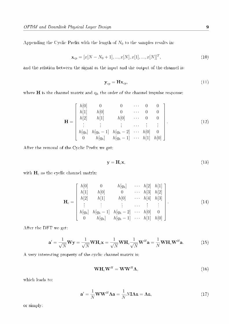
Appending the Cyclic Pre�x with the length of N0 to the samples results in:

xcp = [x[N −N0 + 1], ..., x[N ], x[1], ..., x[N ]]T , (10)

and the relation between the signal at the input and the output of the channel is:

ycp = Hxcp, (11)

where H is the channel matrix and qh the order of the channel impulse response:

H =

h[0] 0 0 · · · 0 0

h[1] h[0] 0 · · · 0 0

h[2] h[1] h[0] · · · 0 0...

...... · · · ...

...h[qh] h[qh − 1] h[qh − 2] · · · h[0] 0

0 h[qh] h[qh − 1] · · · h[1] h[0]

. (12)

After the removal of the Cyclic Pre�x we get:

y = Hcx, (13)

with Hc as the cyclic channel matrix:

Hc =

h[0] 0 h[qh] · · · h[2] h[1]

h[1] h[0] 0 · · · h[3] h[2]

h[2] h[1] h[0] · · · h[4] h[3]...

...... · · · ...

...h[qh] h[qh − 1] h[qh − 2] · · · h[0] 0

0 h[qh] h[qh − 1] · · · h[1] h[0]

. (14)

After the DFT we get:

a′ =1√NWy =

1√NWHcx =

1√NWHc

1√NWHa =

1

NWHcW

Ha. (15)

A very interesting property of the cyclic channel matrix is:

WHcWH = WWHΛ, (16)

which leads to:

a′ =1

NWWHΛa =

1

NNIΛa = Λa, (17)

or simply:

10 Shahram Zarei

a′ = Λ a, (18)

Λ = diag(λ1, λ2, . . . , λN), (19)

λi =qh∑µ=0

h[µ] e−j2πµ(i−1)

N , with i ∈ {1, 2, ..., N}. (20)

The λi are the DFT coe�cients of the channel or the eigenvalues of the channel coe�cientmatrix.

At this point we have derived a very important feature of ODFM with Cyclic Pre�x, namelythat the communication chain reduces to a diagonal matrix with the DFT of the channelcoe�cients as diagonal elements, which means, if we want to equalize the channel, we have tomultiply by the inverse of this diagonal matrix, which is also a diagonal matrix with inverteddiagonal elements. In other words, we can simply multiply each output of the DFT module byits inverted channel coe�cient.

2.8 OFDM system parameter dimensioning

An OFDM system has some key parameters, which have to be designed correctly depending onthe considering scenario. The design parameters of OFDM are:

• ∆f : Subcarrier spacing

⇒ Demand in order to keep Doppler caused ICI low: ∆f � fdmax , fdmax : Max. Dopplershift

• TCP : Length of the Cyclic Pre�x

⇒ To prevent ISI: TCP ≥ Td, Td: Length of the channel impulse response

⇒ Demand for high spectral e�ciency: TCP � T , T: OFDM symbol duration

• N : Number of subcarriers

⇒ N < B∆f , B: OFDM signal bandwidth

The physical layer parameters of the LTE downlink are summarized in Fig. 10.

The technology used in LTE downlink is OFDMA, which stands for Orthogonal FrequencyDivision Multiple Access. In OFDMA, in contrast to OFDM, di�erent subcarriers can beassigned to di�erent users.

OFDM and Downlink Physical Layer Design 11

Figure 10: LTE downlink physical layer parameters

2.9 OFDM drawbacks

OFDM has two main disadvantages:

• PAPR (or crest factor): Stands for Peak-to-Average Power Ratio and can be formulatedas follows:

PAPR =max{|x[n]|2}E{|x[n]|2}

(21)

Power ampli�ers for signals with high PAPR should be highly linear over a broad range.This makes the transmitters expensive. There are several solutions to overcome thisproblem. The �rst and the simplest one is to use power ampli�ers with large back o�e.g. using a 1 kW ampli�er for 100 W output power. This, however, is quite ine�cient.The second solution is to use algorithms, which reduce the PAPR without disturbing themain information content of the signal. Of course there is a certain signal processingcomplexity with PAPR reduction algorithms.

• Sensitivity to frequency o�sets: The second disadvantage of OFDM systems is their highsensitivity to frequency o�sets. This e�ect can be seen in Fig. 11 and 12. As we can see inFig. 12, if there is a frequency o�set between transmitter and receiver, the subcarriers arenot orthogonal to each other anymore and this causes ICI (Inter Carrier Interference). Toavoid this the local oscillator in the receiver should be well synchronized to the transmitterfrequency.

12 Shahram Zarei

Figure 11: Zero ICI

Figure 12: Nonzero ICI if some frequency o�set is present

OFDM and Downlink Physical Layer Design 13

3 Physical layer in downlink

3.1 LTE signal in time domain: Generic frame structure

The LTE signal in time domain is based on frames, which are 10 ms long and consist of 10subframes each of 1 ms duration. The subframes are divided further into two slots each 0.5 mslong. In each slot 7 or 6 OFDM symbols are contained depending on whether normal or shortCyclic Pre�x is used, cf. [1]. The time domain frame structure of the LTE downlink can beseen in the Fig. 13.

Figure 13: LTE downlink signal structure in time domain

3.2 Resource management in LTE downlink physical layer

LTE uses a three dimensional space to manage the resources time, frequency and space (an-tennas). In Fig. 14 only time and frequency dimensions are shown. The smallest unit is theso-called Resource Element (RE), which consists of a time interval of duration of one OFDMsymbol and one subcarrier. Seven OFDM symbols (in case of normal CP length) or 6 symbols(in case of long CP length) build a time slot. The area consisting of 12 subcarriers (180 kHz)and one time slot is called Resource Block and contains 12x7=84 Resource Elements in case ofnormal Cyclic Pre�x.

Figure 14: Resource management in LTE downlink

14 Shahram Zarei

3.3 Downlink reference symbols

In each Resource Block four so-called reference symbols are transmitted. The position of thereference symbols can be seen in the Fig. 15, cf. [7]. The main task of the reference symbolscan be summarized as given below:

• Cell search and initial aquisition

• Channel estimation

• Coherent detection

• Channel quality estimation

Figure 15: Reference symbols in LTE downlink

3.4 LTE downlink signal generation chain

In Fig. 16 the components of the downlink physical layer signal generation chain can be seen.First a 24 bit CRC (Cyclic Redundancy Check) �eld is introduced to detect errors in thereceiver. After the CRC module comes a turbo encoder as forward error correction (FEC)channel coder. The LTE downlink turbo encoder has R = 1/3 as basic code rate and is (canbe) with puncturing. There is an HARQ module following the turbo encoder. HARQ standsfor Hybrid Automatic Repeat Request and is a mechanism based on stop and wait ARQ whichtransmits the packets again in case of errors detected by the CRC. In order to achieve morecoding gain, a scrambling module based on a 31 bit Gold sequence is used after the HARQmodule. The �nal module is the modulator, which can use QPSK, 16QAM or 64QAM in LTEdownlink, cf. [1].

OFDM and Downlink Physical Layer Design 15

In LTE there is the possibility to use MIMO. In this case an antenna mapping module decideson which antenna the packets are to be sent. In LTE downlink up to 4 antennas can be used.

Finally the resource management module selects the appropriate resources, which are in LTEtime slots and subcarriers to transmit the packet.

Figure 16: Signal generation chain in LTE downlink physical layer

3.5 MIMO in LTE

One of the important technologies used in LTE downlink is MIMO. MIMO stands for Multiple-Input Multiple-Output. In MIMO systems, independent parts of a data block are sent overuncorrelated antennas (with a minimum distance greater than e.g. 10λ to ensure uncorrelated-ness). The number of transmit and receive antennas can vary from 1 to 4. For example a 4x4system MIMO has four TX and four RX antennas. MIMO exploits the independency of thescattered signal components in a radio channel und makes some data rate gain possible. Thegreater the independencies between di�erent paths in a channel with scattering, the higher theachieved data rate gains.

Example: Downlink peak data rates (64QAM):

• MIMO (2x2): 172.8 Mbps

• MIMO (4x4): 326.4 Mbps

16 Shahram Zarei

Figure 17: MIMO in LTE

3.6 Summary

• LTE is a high performance technology for mobile broadband services.

• OFDMA is the key core of the LTE downlink physical layer and makes signi�cantly higherdata rates possible.

• With higher order modulation schemes (up to 64QAM), greater spectrum e�ciency isachievable .

• With the MIMO feature, the scattering behavior of the channel is used to increase datarate even more.

References

[1] E. Dahlman, S. Parkvall, J. Sköld, P. Beming: 3G Evolution: HSDPA und LTE formobile broadband, 2007, Academic Press.

[2] S. Sesia, I. Tou�k, M. Baker: LTE - The UMTS Long Term Evolution: From Theoryto Practice, 2009, John Wiley Sons.

[3] W. Koch: Lecture script "Fundamentals of Mobile Communications", 2008, Universityof Erlangen-Nuremberg.

[4] R. Fischer, J. Huber: Skriptum zur Vorlesung "Digitale Übertragung", 2009, Univer-sity of Erlangen-Nuremberg.

[5] U. Barth: 3GPP Long Term Evolution / System architecture evolution overview,2006, Alcatel.

[6] J. Zyren, W. McCoy: Overview of the 3GPP Long Term Evolution physical layer

[7] E. Seidel, V. Pauli: Nomor 3GPP Newsletter, Overview LTE PHY, Nomor Research