Stochastic domain decomposition for the solution

of the two-dimensional magnetotelluric problem

Alexander Bihlo†, Colin G. Farquharson‡, Ronald D. Haynes†

and J. Concepcion Loredo-Osti†

† Department of Mathematics and Statistics, Memorial University of Newfoundland,St. John’s (NL) A1C 5S7, Canada

‡ Department of Earth Sciences, Memorial University of Newfoundland,St. John’s (NL) A1B 3X5, Canada

E-mail: abihlo@mun.ca, cgfarquh@mun.ca, rhaynes@mun.ca, jcloredoosti@mun.ca

Stochastic domain decomposition is proposed as a novel method for solving the two-dimensionalMaxwell’s equations as used in the magnetotelluric method. The stochastic form of the exactsolution of Maxwell’s equations is evaluated using Monte-Carlo methods taking into considerationthat the domain may be divided into neighboring sub-domains. These sub-domains can be natu-rally chosen by splitting the sub-surface domain into regions of constant (or at least continuous)conductivity. The solution over each sub-domain is obtained by solving Maxwell’s equations inthe strong form. The sub-domain solver used for this purpose is a meshless method resting onradial basis function based finite differences. The method is demonstrated by solving a numberof classical magnetotelluric problems, including the quarter-space problem, the block-in-half-spaceproblem and the triangle-in-half-space problem.

1 Introduction

The magnetotelluric method is a standard remote sensing method for inferring the Earth sub-surface electric structure by measuring, at the Earth’s surface, the electro-magnetic fields arisingfrom electric currents induced in the sub-surface by naturally occurring time variations of theEarth’s magnetic field. Due to its potential of probing the sub-surface conductivity structure upto several hundred kilometres, the magnetotelluric method has become a standard technique forexploration surveys aiming at locating mineral and hydrocarbon resources, and for investigatingthe structure and composition of the Earth’s crust and upper mantle [8, 33].

Linking the data obtained from field surveys to the conductivity structure in the groundrequires a numerical solution of Maxwell’s equations. Several techniques have been proposed forthis purpose, including finite difference, finite volume and finite element solvers [35,38]. In thispaper we propose another method suitable for the numerical evaluation of Maxwell’s equations,based on stochastic domain decomposition [1], that is particularly suited to efficient computationvia parallelization and that has the potential to handle arbitrary topography and realisticallycomplex geological interfaces.

Stochastic domain decomposition is a relatively recent domain decomposition method. Intraditional (deterministic) domain decomposition one generally splits the physical domain intosub-domains and alternately (or in parallel) solves the given differential equation over eachsub-domain. Proper interface conditions between the sub-domains ensure convergence of thedomain decomposition procedure to the global solution over the entire domain using an iterationprocedure. The rate of convergence strongly depends on what type of interface conditions arechosen, see e.g. [30], and finding the most optimized interface conditions is usually a challengingtask.

In contrast to traditional domain decomposition, stochastic domain decomposition does notrequire iteration. The main requirement for the applicability of stochastic domain decompositionis that the partial differential equation under consideration possesses a stochastic representationof its exact solution. This is always the case for linear elliptic boundary value problems and

1

arX

iv:1

603.

0931

1v1

[ph

ysic

s.ge

o-ph

] 3

0 M

ar 2

016

linear parabolic initial–boundary value problems [19]. Certain nonlinear differential equationsalso allow for a stochastic representation of their exact solution, see e.g. [2].

The probabilistic form of the exact solution of a differential equation can be evaluated nu-merically using Monte-Carlo methods. While Monte-Carlo methods are known to convergenotoriously slowly and hence only become competitive for higher-dimensional problems [29], thesituation is different in the stochastic domain decomposition framework. Here, one evaluates thestochastic representation of the exact solution only on the interfaces between the sub-domains.Thus, rather than computing the solution of the global problem using the stochastic techniqueat every point, only interface solutions have to be computed. The solution over each individualsub-domain can then be obtained using deterministic methods. Moreover, since the stochasticsolution reproduces the exact solution up to the numerical error (consisting of a time-steppingerror, the boundary hitting error and the Monte-Carlo error [1]), no iteration is required forthe domain decomposition technique to converge. In addition, once the interface solutions areobtained, the sub-domain solutions can be computed over all the sub-domains simultaneouslyand in parallel. Stochastic domain decomposition is thus particularly suited to massively parallelcomputing architectures. Stochastic domain decomposition has been used to solve physical par-tial differential equations in [1–3] and for the generation of moving meshes in partial differentialbased grid generators in [4, 5].

In this paper we apply the stochastic domain decomposition method to the two-dimensionalmagnetotelluric problem, solving the two-dimensional Maxwell’s equation in the time-frequencydomain. The main challenge in applying the method to Maxwell’s equations is the presenceof conductivity jumps. The two-dimensional Maxwell’s equations, as used in the magnetotel-luric method, are a system of differential equations with discontinuous coefficients. This addsanother layer of complexity as most work connecting boundary value problems and stochasticcalculus has been done for equations with continuous coefficients, see e.g. [26]. However, thediscontinuity in the conductivity allows for a natural splitting in sub-domains, namely thosewhere the conductivity is constant (or at least continuous). This enables one to solve Maxwell’sequations in the strong form on each of the sub-domains, which is the route that we will pursuein this paper. For a recent exposition on a deterministic domain decomposition method for thethree-dimensional time-dependent Maxwell’s equations, see [10].

Since the stochastic form of the exact solution of Maxwell’s equations can be evaluated atarbitrary points, and in realistic sub-surface models the conductivity jumps can have arbitraryshape, it is natural to use a deterministic sub-domain solver that can handle a variety of interfacelayouts as well. This makes so-called meshfree methods a natural choice. The use of meshfreemethods in geophysics is relatively recent. The magnetotelluric problem has been consideredquite recently in this light in [36], although there the authors used the Maxwell’s equation inthe weak form. This requires one to use high order numerical integration which can be avoidedif meshless methods in the strong form are invoked. In the present paper, we will use radialbasis function based finite differences (RBF-FD). This is a prominent meshless method [14, 16]that is in some sense a generalization of the traditional finite difference method, replacing thetraditional polynomial basis functions with radial basis functions. The method is truly meshless,i.e. it can be used on arbitrarily distributed nodes.

This paper is organized as follows. In Section 2 we present the mathematical background un-derlying the stochastic domain decomposition method for the two-dimensional Maxwell’s equa-tions. This includes both a discussion of the stochastic representation of the exact solution ofMaxwell’s equations and the description of the numerical evaluation of this representation inthe context of stochastic domain decomposition. Section 3 details the numerical implementa-tion of the stochastic domain decomposition method. This concerns both the choice for thediscretization of the stochastic representation of the exact solution of Maxwell’s equations, andthe implementational details of the RBF-FD method. Numerical results for an analytical so-lution and some simple geophysical examples are presented in Section 4. Although simple,

2

these traditional tests show the potential of the stochastic domain decomposition method. Theconclusion and final thoughts are given in Section 5.

2 Stochastic domain decomposition for thetwo-dimensional Maxwell’s equations

In this section we present the necessary theoretical background underlying the stochastic do-main decomposition for the quasi-static two-dimensional Maxwell’s equations as used in themagnetotelluric method.

2.1 The two-dimensional Maxwell’s equations

The two-dimensional quasi-static Maxwell’s in the time frequency domain read

∇ ·(

1

iωµ∇Ey

)− σEy = 0, ∇ ·

(1

σ∇Hy

)− iωµHy = 0, (1)

where ∇ = (∂x, ∂z) is the two-dimensional gradient operator in the (x, z)-plane, Ey and Hy

are the y-components of the electric and magnetic field vectors E and H, respectively, σ is theelectric conductivity, µ = µ0 = 4 · 10−7 Hm−1 is the magnetic permeability, ω is the angularfrequency, and i =

√−1 is the imaginary unit. The equation for the electric field component

is called the TE-mode, whereas the equation for the magnetic field component is called theTM-mode.

The above system (1) gives the components of the primary fields perpendicular to the planeof the model, from which the secondary field components Ex and Hx in the plane of the modelcan be derived as

Ex =1

σ

∂Hy

∂z, Hx = − 1

iωµ

∂Ey

∂z. (2)

The system for the field components Ex, Ey, Hx and Hy has to be complemented with appro-priate boundary conditions. In the following we will work with Dirichlet boundary conditionsexclusively. More precisely, we will assume that all the boundaries are far away from any regionsof anomalous conductivity so that the one-dimensional half-space boundary conditions can beused on the left and on the right of the domain [34, p. 56; Figure 1]. The top and bottomboundaries are obtained from linear interpolation from the respective top and bottom cornerpoints of the domain, respectively.

x

z

σ(x , z )

σ0

σ1

Figure 1: A sample subsurface structure and computational domain for system (1).

3

The proposed stochastic domain decomposition method can also be applied to other kinds ofboundary conditions, including Neumann and Robin boundary conditions. For further details,see [24].

Once the primary and secondary field components are computed, they can be used to calculatethe apparent resistivities and phases as

ρTEa =

1

ωµ

∣∣∣∣EyHx

∣∣∣∣2 and ϕTE = arg

(Ey

Hx

),

ρTMa =

1

ωµ

∣∣∣∣ExHy

∣∣∣∣2 and ϕTM = arg

(Ex

Hy

).

(3)

2.2 Stochastic analysis for the two-dimensional Maxwell’s equations

For a given domain Ω ⊂ R2, it is well-known that for linear elliptic boundary value problems ofthe form

Lu− λ(x, z)u = 0 in Ω, u|∂Ω = g(x, z), (4)

where λ is non-negative and L = 12aij(x, z)∂i∂j + bi(x, z)∂i is a semi-elliptic operator with

bounded, two times continuously differentiable coefficients (summation over repeated indices isimplied), the exact solution can be written in probabilistic form as

u(x, z) = E

(g(β(τ∂Ω)) exp

(−∫ τ∂Ω

0λ(β(s)) ds

) ∣∣∣β(0) = (x, z)

). (5a)

Here, β(t) = (X(t), Z(t)) denotes the stochastic process associated with the operator L, satis-fying the stochastic differential equation

dβ = b(β)dt+ V (β)dW, (5b)

where the two-dimensional drift vector b has components b1, b2, and the 2×2 matrices V = (Vij)and a = (aij) are related through V V T = a, and W is two-dimensional Brownian motion. Byτ∂Ω we denote the first hitting time of the boundary of Ω for a stochastic process β(t) startingat point (x, z). Eq. (5a) is the celebrated Kac–Feynman formula [26].

The main problem in using the stochastic solution (5) is that the two-dimensional Maxwell’sequations are not of the form of (4) since the conductivity σ is in general not a continuousfunction. It is therefore necessary to study the class of problems given by

1

2∇ · (κ(x, z)∇u)− λ(x, z)u = 0 in Ω, u|∂Ω = g(x, z), (6)

where both κ and λ are discontinuous. For the two-dimensional Maxwell’s equations we haveκ = 2/(iωµ) and λ = σ for the TE-mode and κ = 2/σ and λ = iωµ for the TM-mode. That is, λis discontinuous for the TE-mode and κ is discontinuous for the TM-mode, and both parameterscan be complex-valued. Multiplying the equation for the electric mode with i, it is sufficient toassume that κ ∈ R+ and λ ∈ C.

The stochastic analysis of this class of problems is considerably more elaborate; availabletheoretical results seem to be mostly restricted to one-dimensional and real-valued cases. Whileit follows from applying a regularization argument, see e.g. [20], that the solution of Eq. (6) is stillgiven through the Kac–Feynman formula (5a), finding a suitable stochastic process associatedwith the operator 1

2∇ · (κ(x, z)∇) for general forms of discontinuous κ appears to be an openproblem.

On the other hand, the construction of numerical approximations to this problem for the caseof κ (and λ) being piecewise constant has been the subject of several investigations, especially

4

for the case of λ = 0. See [6,22,24,31] for recent results. Different schemes have been proposed,which include so-called kinetic schemes [21], mixing schemes [22], schemes relying on occupationtimes [20] and schemes using ideas of finite differences [22, 25]. Here, we have chosen this lastapproach and will discuss it in more detail.

The main idea of all the above approaches is to split the domain into sub-domains Ωi overwhich both κ and λ are constant. On each sub-domain, Eq. (6) reduces to

1

2κi∆u− λiu = 0 in Ωi. (7)

This equation is of the form (4) and hence the stochastic solution as given by (5) holds. Moreprecisely, the stochastic differential equation (5b) simplifies to

dβ =√κi IΩi(β) dW, (8)

where here and in the following IA is the indicator function of A. This means that the processcan be simulated via regular Brownian motion when it is away from the interface. If it reachesthe interface, it is possible that for a while the process goes to and fro between adjacent sub-domains before it randomly resolves in either direction. The issue is that when the diffusioncoefficients are different, every time that the process crosses the interface, the regime changes.

The approximation of the β(t) process as it passes through the interface can be based onfinite differences by imposing the condition of continuity of the flux κ∇u across the interface,

κi∇u = κj∇u at γij , (9)

where γij is the interface between the neighboring sub-domains Ωi and Ωj .Without loss of generality, we assume that there is only one vertical interface separating the

two neighboring sub-domains Ω1 and Ω2 located at x = 0. At this interface, the continuity ofthe flux condition (9) can be represented as

κ1 limh1→0

u(h1, z)− u(0, z)

h1= κ2 lim

h2→0

u(−h2, z)− u(0, z)

−h2, ∀(0, z) ∈ γ, (10)

which can be locally solved for u(0, z) yielding

u(0, z) ≈ p1u(h1, z) + p2u(−h2, z), h1, h2 > 0, (11)

with

p1 =κ1h2

κ1h2 + κ2h1, p2 =

κ2h1

κ1h2 + κ2h1.

If h1 = h2 = h, then,

p1 =κ1

κ1 + κ2, p2 =

κ2

κ1 + κ2. (12)

An interpretation of the above formula (11) is that when the β(t) process reaches the interface,locally, u(0, z) can be approximated as the expected value of a random variable taking valuesu(h1, z) and u(−h2, z) with probabilities p1 and p2, respectively. This, in turn, also admitsthe following probabilistic interpretation: after reaching the interface, the process resumes fromeither, a point in the neighborhood of (h1, z) with probability p1, or the neighborhood of (−h2, z)with probability p2. This interpretation provides a straightforward algorithm to deal with theprocess when it hits the interface. Note that formula (11) is not exact as long as h1, h2 are finite.

An alternative to the previous procedure consists of dissecting the behaviour of the processas it moves through the interface by using notions of Skew Brownian motion and Brownianmeander, see [20, 23] for further discussions. An algorithm using this alternative approach iscomputationally more complex and expensive than the one based on finite differences. However,our testing indicates that both algorithms produce qualitatively similar results. For this reason,we choose to present only the procedure which is easier to implement.

5

3 Numerical implementation

In this section we present the details of the novel numerical implementation of stochastic domaindecomposition for the two-dimensional Maxwell’s equations in the frequency domain.

3.1 Stochastic solver

The pointwise stochastic solution procedure consists of simulating realizations of the path β(n),β(n) =

(β

(n)x , β

(n)z

), a discretized version of the solution to the differential equation (8) based

on a modification of the Euler–Maruyama method. The starting position, β0 = (x, z), is thepoint at which the numerical solution is sought and the realization of the process is completedwhen the overall boundary of Ω is reached. Suppose that at the step n the process is in thesub-domain Ωi. Then, we draw a provisional β(n+1) as

β(n+1) = β(n) +√κi ∆tW, W ∼ N (0, I2) (13)

where ∆t = t(n+1) − t(n) is the time step, and N (0, I2) denotes the distribution of a random2-vector of independent standard normal variables. Next, we check if ∂Ω has been reached. Ifso, the realization is completed. Otherwise, we verify whether between the times t(n) and t(n+1)

the interface has been hit. If the process is away from the interface, β(n+1) is retained and ∆tis added to Ti, the occupation time of Ωi, before moving on to the next iteration.

When the process hits an interface point (x, z)|γij , say (xγij , z), if κi 6= κj , we carry out theprocedure laid out in Section 2.2, i.e., by using the probabilities pi and pj = 1 − pi from (12),we randomize to determine whether β(n+1) lies in Ωi or in Ωj . Also, we estimate the occupationtimes between t(n) and t(n+1). First, by either inverting the test for the first hitting time duringan excursion with respect to a Brownian bridge (i.e., when the provisional β(n+1) is on the samesub-domain as β(n)), or approximating the expected value of the first exit time with respect toa Brownian bridge, we estimate the time when the interface was first reached [7,18]. We define

t(n)γij as

t(n)γij =

−2(β

(n)x − xγij )(β

(n+1)x − xγij )

κi logUγ, Uγ ∼ U(0, 1), if β(n), β(n+1) in Ωi

∆t

∣∣∣∣∣ β(n)x − xγij

β(n+1)x − β(n)

x

∣∣∣∣∣ , if β(n) in Ωi and β(n+1) in Ωj ,

(14)

where U(0, 1) denotes the uniform distribution on [0, 1], so that whenever t(n)γij ≤ ∆t, we con-

clude that the process has reached the interface at time t(n) + t(n)γij and, accordingly, proceed to

randomize in order to find the definitive value for β(n+1). This randomization and the updateof the occupation times can be done as follows. Let cij(h) be

cij(h) = h I[β

(n)x ≤xγij

] − h I[β

(n)x >xγij

].Now, if Uα < pi, Uα ∼ U(0, 1), then β(n+1) is drawn randomly from inside a circle of radius

hi and center(xγij − cij(hi), z

), and ∆t − 1

2

(∆t− t(n)

γij

)pi and 1

2

(∆t− t(n)

γij

)pi are added to

Ti and Tj , respectively. Otherwise, β(n+1) is drawn from a circle with radius hj and center(xγij + cij(hj), z

), and t

(n)γij + 1

2

(∆t− t(n)

γij

)pj and 1

2

(∆t− t(n)

γij

)(1 + pj) are added to Ti and Tj ,

respectively. These occupation times estimates are based on approximations of their expectedvalue as the process moves around the interface given γij [20]. When κi = κj and the processhits the γij interface, there is no regime change and we retain β(n+1) obtained through (13).Only the occupation times between t(n) and t(n+1) are updated according to where β(n+1) lies.

6

This process is repeated N times so that the expected value appearing in (5a) can be ap-proximated as

u(x, z) =1

N

N∑r=1

g(βr(τr)) exp

− K∑j=1

λkTrj

,

where βr(τr) denotes the state of the process at the time τr of the rth realization of the discretizedprocess (13), τr is the time estimate at which the overall boundary, ∂Ω, was first reached, K isthe number of sub-domains Ωj with different κj (and/or λj) and T rj is the time spent in the jthsub-domain through the rth realization. When ∂Ω consists of vertical or horizontal barriers, theestimation of τr, the first exit time from Ω for the rth realization of the process, can be carried

through an expression similar to (14) with (x, z)|γij replaced by (x, z)|∂Ω. Thus, when t(n)∂Ω ≤ ∆t,

we conclude that the process has reached the boundary at time τr = t(n) + t(n)∂Ω bringing the rth

realization of the process to an end.

Remark 1. While the main aim of this paper is to put forward a new method for solving thetwo-dimensional Maxwell’s equations over the entire computational domain, the stochastic formof the solution of Maxwell’s equations can also be used to compute the solution in single, isolatedpoints. Thus, if the solution is only required near the measurement sites, the stochastic solutioncan be used for this purpose as well. This is in striking contrast to all deterministic methods,which require the computations to be carried out over the entire domain, even if the solution isonly required in a single point. An example for this use will be presented in Section 4.

3.2 Sub-domain solver

Since we are primarily interested in the application of the stochastic domain decompositionmethods to the two-dimensional Maxwell’s equations for realistic sub-surface models, the singlesub-domains Ωi will generally be of an arbitrary shape. This makes it natural to choose a sub-domain solver that can operate on an arbitrary set of mesh points distributed in a suitable wayover the single sub-domain. This makes meshless methods a suitable choice.

The underlying paradigm of meshless methods is that one does not require a topologicallyconnected mesh in order to compute a numerical solution over a given domain, as is requiredin conventional mesh-based methods such as finite differences, finite volumes or finite elements.In meshless methods, the local approximations of derivatives are formulated directly in terms of(in principle) arbitrarily distributed nodes. Various meshfree methods have been developed overthe past few decades, including smooth particle hydrodynamics, meshless finite differences, ra-dial basis function methods, meshless local Petrov–Galerkin methods and element-free Galerkinmethods [9, 14,26,27].

In this paper we will use the radial basis function based finite differences method (RBF-FD).This method rests on replacing the one-dimensional polynomial test functions that are used toderive regular finite difference formulas by radial basis functions (RBFs) [16]. More precisely,the weights wi at the node locations xi, i = 1, . . . , n required to approximate a linear differentialoperator L at the node x0 are obtained by solving the matrix system

φ(||x1 − x1||) φ(||x1 − x2||) · · · φ(||x1 − xn||)φ(||x2 − x1||) φ(||x2 − x2||) · · · φ(||x2 − xn||)

......

...φ(||xn − x1||) φ(||xn − x2||) · · · φ(||xn − xn||)

w1

w2...wn

=

Lφ(||x− x1||)|x=x0

Lφ(||x− x2||)|x=x0

...Lφ(||x− xn||)|x=x0

.

In other words, the weights are found in the RBF-FD method by requiring that the approx-imation of L is exact when applied to the radial basis functions themselves. Here, xi =

7

(x1i , x

2i , · · · , xdi )T is a point in d-dimensional space, || · || is the Euclidean 2-norm and φ(||x−xi||)

is an RBF centered at the node xi.Common RBFs used in practice include the Gaussian, φ(r) = exp(−(εr)2), the multiquadric,

φ(r) =√

1 + (εr)2, and the inverse multiquadric, φ(r) = (1 + (εr)2)−1/2 [16]. The parameter εis called the shape parameter and it controls the flatness of the RBF. In the following, we willuse the multiquadric for all computations.

For the given RBFs the above matrix system can be solved provided that the nodes xi,i = 1, . . . , n are distinct. Denoting by A the matrix with elements Aij = φ(||xi − xj ||) andby B the square matrix with elements Bij = Lφ(||x − xj ||)|x=xi the differentiation matrix Dapproximating the linear operator L becomes

D = BTA−1.

In other words, for the action of L on a function f(x), we have the following approximationLf(x)|x=x1

Lf(x)|x=x2

...Lf(x)|x=xn

≈ D

f(x1)f(x2)

...f(xn)

.

A main problem with the above procedure is that the differentiation matrix D is a full matrix.Its computation requires O(n3) operations, which is very costly if D has to be re-computed. Thishappens, for example, if the node layout xi changes, which is always necessary for movingmesh methods or if adaptive mesh refinement is used.

A more cost efficient way is achieved by assigning to each of the n nodes, xi, a separate stencilof ns n nodes. These nodes are typically the ns − 1 nearest neighbors of each node x0. Inthis procedure, the differentiation matrix D becomes a sparse matrix having ns non-zero entriesin each of the n rows. This restriction to neighboring nodes yields the RBF-FD method. It isthe exact analogue of the classical finite difference method, using RBFs instead of polynomialsas basis functions in the stencil around each point x0.

For Maxwell’s equations, we require to approximate L = ∆ on each sub-domain with continu-ous conductivity. We do this by creating separate differentiation matrices for L = ∂2

x and L = ∂2z

using ns = 9 nodes per each stencil. These nodes are chosen to be the 8 nearest neighbors andthe center node x0 itself.

The choice of the shape parameter ε is paramount in that it governs the accuracy of the RBF-FD method. It is generally found that the numerical computations become most accurate whenusing almost flat RBFs (i.e. ε being very small). The smaller the parameter ε, however, the moreill-conditioned the matrix systems become [17,37]. In order to overcome the dilemma of choosingbetween accuracy and ill-conditioning, several methods have been proposed, including the useof high precision arithmetics and the RBF-QR method [15], which was mostly developed forGaussian RBFs. We found experimentally that a value of ε = 1/2000 gives satisfying accuracyfor a wide range of grid spacings in the test problems considered in the following section. A morethorough investigation of the optimal shape parameter ε for use within the stochastic domaindecomposition method for Maxwell’s equations should be investigated elsewhere.

4 Results

In this section we present numerical results using the stochastic solution technique for the two-dimensional Maxwell’s equations discussed in the previous section. These examples are well-studied in the literature and serve as a demonstration for the potential of the new method tocorrectly reproduce existing results. More realistic sub-surface models that will also demonstrateof the full potential of the meshless RBF-FD method will be presented in a separate paper.

8

4.1 Analytical test model

To verify numerically our method for evaluating the process as it passes through the interfacefor discontinuous κ and imaginary λ, we consider the Dirichlet problem for the complex-valuedHelmholtz equation

∇ · (κ∇)u+ λu = 0, (15a)

with exact solution

ue = c1(z + c2)

cosh(√

λκ1x), −1 ≤ x < 0

cosh(√

λκ2x), 0 ≤ x ≤ 1.

(15b)

Here we choose c1 = c2 = 1, κ1 = 1, κ2 = 10 and λ = 10i as parameters. The exact solution ue

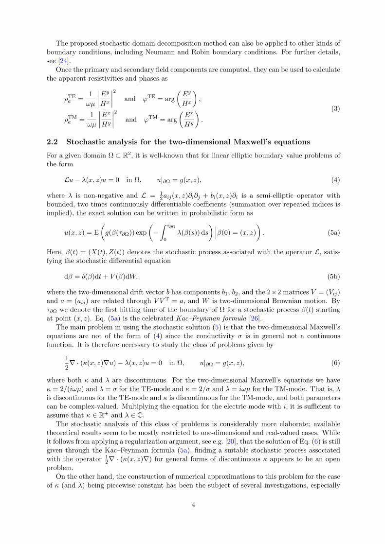
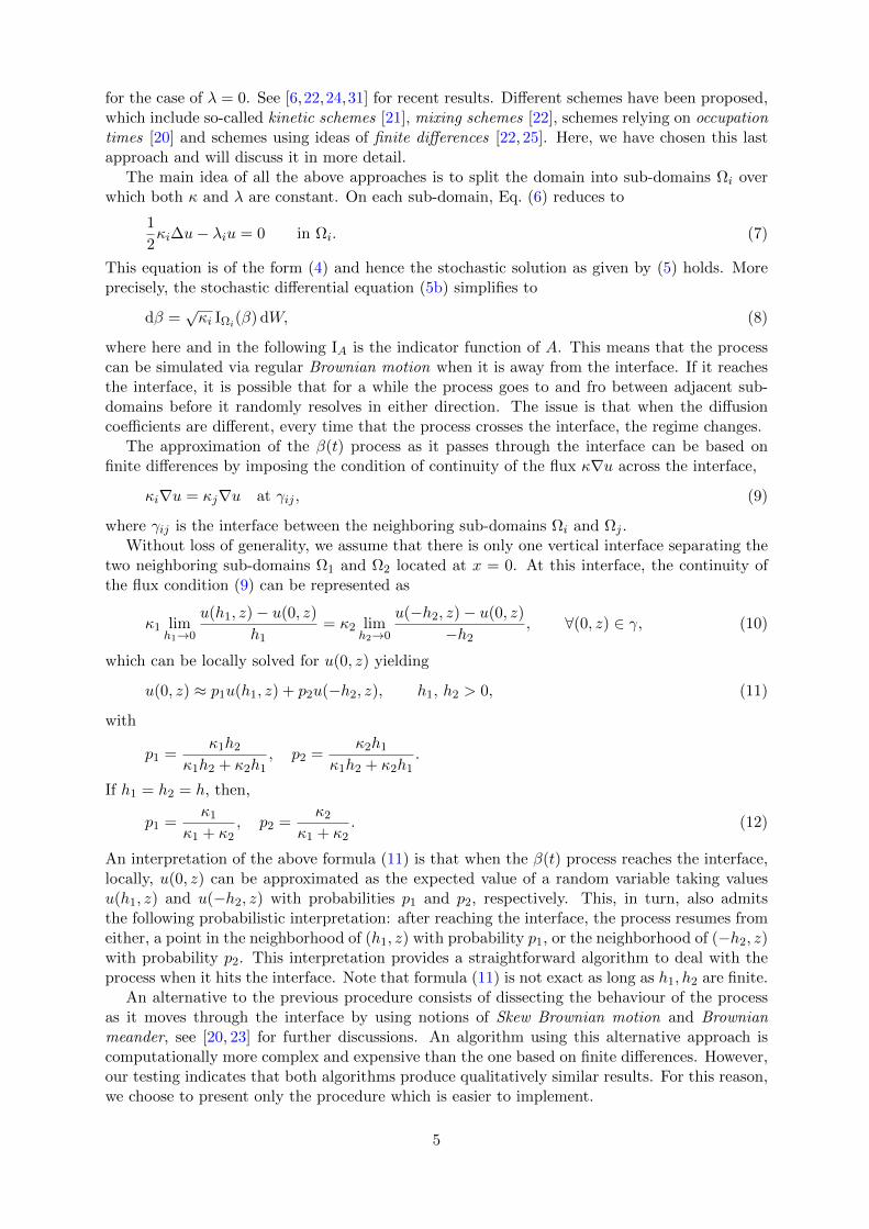
is used as boundary data for the physical domain. The physical domain Ω = [−1, 1] × [−1, 1]is discretized using a uniform mesh with 51 × 51 grid points. The stochastic differential equa-tion (5b) is discretized using the Euler–Maruyama method with time step ∆t ∝ (∆x)2. In Fig. 2we display the numerical solution un obtained from using the stochastic procedure in all gridpoints with N = 10000 Monte-Carlo simulations. The associated point-wise errors are displayedin Fig. 3.

-3

1

-2

-1

0.5 1

0

rea

l(u

n)

1

0.5

z

0

2

x

3

0-0.5

-0.5-1 -1

-4

1

-2

0.5 1

0

ima

g(u

n)

0.5

2

z

0

x

4

0-0.5

-0.5-1 -1

Figure 2: Numerical solution for the analytical test problem using N = 10000 Monte-Carlosimulations. Left: Real part, right: Imaginary part.

In order to show the decrease of the errors as the number of Monte-Carlo simulations, N , isincreased, we present the absolute errors for different values of N in Table 1. Since numericallysolving (15) at every point in Ω is computationally intensive for a study of increasing N , theerrors reported in Table 1 are for the single point (x, z) = (0.6, 0.6) only. While the magnitudeof the error is spatially dependent, the error decrease with increasing N demonstrated below at(0.6, 0.6) remains valid throughout the domain.

Table 1: Absolute errors for the model (15) at point (0.6, 0.6) varying N .

N 1 · 104 1 · 105 1 · 106

<(error) 0.0086 0.0017 7.25 · 10−4

=(error) 0.0067 0.0034 8.95 · 10−4

The convergence results presented in Table 1 should be taken with a grain of salt. Recall thatthe error incurred by numerically evaluating the stochastic representation of an exact solution of

9

-0.04

1

-0.02

0.5 1

0

rea

l(u

n-u

e)

0.5

0.02

z

0

x

0.04

0-0.5

-0.5-1 -1

-0.04

1

-0.02

0

0.5 1

ima

g(u

n-u

e)

0.02

0.5

z

0.04

0

x

0.06

0-0.5

-0.5-1 -1

Figure 3: Error plots for the analytical test problem for N = 10000 Monte-Carlo simulations.Left: Real part, right: Imaginary part.

a linear boundary value problem such as (5) consists of three parts. These are the pure Monte-Carlo error (due to approximating the expected value in Eq. (5a) with the mean value), thetime stepping error (due to discretizing the stochastic differential equation (5b) using a finitetime step), and the error in estimating the first exit time τ∂Ω [1]. Increasing only the numberof Monte-Carlo simulations as done in Table 1 hence will not lead to a convergent numericalscheme unless also the two other sources of errors are controlled, e.g. by using increasingly smalltime steps which will both reduce the time stepping error and improve the estimate for the firstexit time. What Table 1 does demonstrate is that if a reasonably small time step is chosen inthe discretization of the stochastic differential equation (5b) (controlling the second and thirdsources of numerical error), the numerical results obtained can be improved by merely increasingthe number of Monte-Carlo simulations. This also shows that the additional error introduceddue to our approximation strategy at the interface is small enough to prevent error saturationbefore geophysically acceptable accuracy is achieved. This is also explicitly demonstrated in thefollowing examples.

4.2 Quarter-space solution

The quarter-space model for this experiment is identical to the one proposed in [12,13]. It splitsthe region z ≥ 0 into two areas, one with conductivity σ = 0.1S/m (on the left), the other withconductivity σ = 0.01S/m (on the right), see Fig. 4.

z

x

Figure 4: Conductivity model for the quarter-space experiment.

As in [12, 13], we used f = 1 Hz as the frequency. We employed a variable grid spacing with

10

minimum cell sizes being ∆x×∆z = 50 m×50 m near the interfaces and a maximum cell size of∆x×∆z = 300 m×200 m near the boundaries in the ground. A total of N = 5000 Monte-Carlosimulations was used in the stochastic solver, which here and in the following was only usedat the sub-domain interfaces, with the solution over the sub-domains being computed usingthe deterministic, meshless solver. Note that the variable resolution of the model is naturallyhandled using the meshless solver.

The apparent resistivities and phases for the quarter-space model are shown in Fig. 5 and 6,respectively. They align closely with the results presented in [12,13].

−2 −1.5 −1 −0.5 0 0.5 1 1.5 2

x 104

100

101

102

103

x [m]

ρa [

Ω m

]

−2 −1.5 −1 −0.5 0 0.5 1 1.5 2

x 104

100

101

102

103

Figure 5: Apparent resistivities for the TE-mode (left) and the TM-mode (right) for the quarter-space model using f = 1 Hz.

−2.5 −2 −1.5 −1 −0.5 0 0.5 1 1.5 2 2.5

x 104

40

42

44

46

48

50

52

54

56

x [m]

φ [

De

gre

e]

−2.5 −2 −1.5 −1 −0.5 0 0.5 1 1.5 2 2.5

x 104

40

42

44

46

48

50

52

54

56

x [m]

φ [

De

gre

e]

Figure 6: Phases for the TE-mode (left) and the TM-mode (right) for the quarter-space modelusing f = 1 Hz.

4.3 Rectangular block in half-space solution

This experiment coincides with the COMMEMI 2D-1 example [38]. It is given by a symmetrical,rectangular, highly conducting block embedded in an otherwise uniform conducting half-space.More precisely, the rectangular block measures 1000 m in x-direction, 2000 m in z-direction,with its top edge lying at z = 250 m. The conductivity of the block is σ = 2S/m, and theconductivity of the half-space is σ = 0.01S/m. The conductivity model of this test problem isdepicted in Fig. 7. The frequency used in the experiments was f = 10 Hz. We carry out twoexperiments for the COMMEMI 2D-1 model.

11

In the first experiment we obtain a solution to the two-dimensional Maxwell’s equations usingthe stochastic domain decomposition algorithm. For this experiment, the grid cells of the modelwere of size ∆x×∆z = 100 m×125 m throughout the entire domain. The number of Monte-Carlosimulations used in the stochastic solver was N = 5000.

As was outlined in Section 2, the stochastic solution to Maxwell’s equations allows oneto compute the solution at single points only. For the sake of demonstration, in the sec-ond experiment we compute the solution stochastically only in the COMMEMI locations, x ∈0, 500, 1000, 2000, 4000. More specifically, we compute the solution in three points near thesurface at the aforementioned x-locations to be able to compute the required secondary fieldsby evaluating Eqs. (2) using regular centered differences. A total of N = 400000 Monte-Carlosimulations was used in this experiment. This high number of Monte-Carlo simulations ensuresthat the primary fields Ey and Hy are computed with high accuracy to then allow generatingsufficiently accurate approximations for the secondary fields Ex and Hx, yielding accurate valuesfor the apparent resistivities ρTE

a and ρTMa .

2000 m

250 m

1000 m

σ=5 S/m

σ=0.01 S/m

Figure 7: Conductivity model for the COMMEMI 2D-1 experiment.

The apparent resistivities for the TE-mode and TM-mode are shown in Fig. 8.

−5000 0 50000

20

40

60

80

100

120

SDD

Stochastic

COMMEMI

−5000 0 500010

20

30

40

50

60

70

80

90

100

110

SDD

Stochastic

COMMEMI

Figure 8: Apparent resistivities for the TE-mode (left) and the TM-mode (right) for the COM-MEMI 2D-1 experiment using f = 10 Hz.

To give a better comparison with the values reported in the COMMEMI experiments, inTable 2 we list the mean values (and standard deviation) taken from Table B.8 in [38] alongwith the numerical values obtained with our two approaches.

It can be seen from Table 2 that the stochastic domain decomposition method producesvalues that are well within the range of results reported in the COMMEMI experiments. Theonly significant deviation is the value for the TM-mode resistivity at x = 500 m. As can be seen

12

Table 2: Apparent resistivities computed using the SDD method and the purely stochasticalgorithm compared to the original COMMEMI results.

ρa(TM) 0 m 500 m 1000 m 2000 m 4000 m

SDD 10.15 36.01 93.98 98.55 99.78Stochastic 11.58 41.10 93.43 98.52 99.65

COMMEMI 10.13 ± 0.96 48.07 ± 3.65 94.27 ± 0.79 98.40 ± 0.40 99.71 ± 0.64

ρa(TE) 0 m 500 m 1000 m 2000 m 4000 m

SDD 7.44 13.27 51.20 97.58 104.36Stochastic 6.70 12.50 50.84 97.54 103.77

COMMEMI 7.60 ± 1.04 13.92 ± 1.82 50.70 ± 2.48 95.94 ± 2.75 103.92 ± 0.80

from the right plot in Fig. 8, this is the region of highest variability in the resistivity and theCOMMEMI mean is obtained between x = 500 m and the neighboring grid point. Similarly,the point-wise solution obtained using the purely stochastic algorithm also gives results that arewell within the range of the COMMEMI results, demonstrating that if solutions are sought insingle points only, the stochastic algorithm may be a viable alternative compared to standarddeterministic methods that requires the computation of the numerical solution over the entiredomain even if the solution is required at several points only.

4.4 Triangular block in half-space solution

This experiment was previously considered in [11]. It is a bit more general than the COMMEMI2D-1 example and, with the sloping interface of the triangular anomaly, begins to illustratethe capability of the combination of the domain-decomposition solver and the meshless sub-domain solver to take into account arbitrary, complex interfaces. The conductivity model forthis example is illustrated in Fig. 9. The triangle has corners at the three points (−600, 400),(−600, 2500) and (1500, 2500) with conductivity σ = 0.2S/m in a half-space with conductivityσ = 0.01S/m.

The grid cells for this model were of size ∆x×∆z = 100 m×50 m and N = 5000 Monte-Carlosimulations were used for the approximation of the expected values. For this experiment, weused the frequencies f = 1 Hz, f = 3 Hz and f = 10 Hz.

2000 m

500 m

2000 m

σ=0.2 S/m

σ=0.01 S/m

Figure 9: Conductivity model for the triangle in a half-space example.

The conductivities and phases for this experiment are displayed in Fig. 10 and Fig. 11. Herewe present the results using the SDD method and the model developed in [11].

It can be seen from Fig. 10 and Fig. 11 that for the TE-mode the apparent resistivitiesand phases for both methods coincide closely. For the TM-mode the results do not coincide aswell, with the discrepancy increasing as the frequency increases. The reason for this is that the

13

−4000 −3000 −2000 −1000 0 1000 2000 3000 400020

30

40

50

60

70

80

90

100

110

x [m]

ρa [

Ω m

]

SDD 1 Hz

Det 1 Hz

SDD 3 Hz

Det 3 Hz

SDD 10 Hz

Det 10 Hz

−4000 −3000 −2000 −1000 0 1000 2000 3000 400040

50

60

70

80

90

100

110

x [m]

ρa [

Ω m

]

SDD 1 Hz

Det 1 Hz

SDD 3 Hz

Det 3 Hz

SDD 10 Hz

Det 10 Hz

Figure 10: Apparent resistivities for the TE-mode (left) and the TM-mode (right) for the trianglein a half-space experiment. Results from the SDD model (circles) and the deterministic modelpresented in [11] for the frequencies f = 1 Hz, f = 3 Hz and f = 10 Hz.

Figure 11: Phases for the TE-mode (left) and the TM-mode (right) for the triangle in a half-space experiment. Results from the SDD model (circles) and the model presented in [11] for thefrequencies f = 1 Hz, f = 3 Hz and f = 10 Hz.

conductivity model is treated differently by the different methods. For the stochastic domaindecomposition approach presented here, a conductivity is associated with each node, with thisconductivity being implicitly an average over the neighbourhood of the node. For the FD schemeof [11], the conductivity is explicitly considered to be uniform throughout each rectangular cellof the mesh with the approximate values for Ex and Hx solved for at cell centers and cell vertices(for the TE- and TM-modes respectively).

5 Conclusion

The present paper introduced the stochastic domain decomposition method for solving the two-dimensional Maxwell’s equations as required in the magnetotelluric method. The method isnew in that it allows splitting of the sub-surface into regions of constant or continuous conduc-tivity, over which Maxwell’s equations can be solved independently. This splitting also allowsone to use the strong form of Maxwell’s equations and thus the potential costly numerical in-tegrations required in solvers using the weak form can be avoided. The interface solutions forthese sub-domains are naturally found by evaluating the stochastic form of Maxwell’s equations

14

numerically using Monte-Carlo techniques. Once these interface values have been computed,any sub-domain solver can be used to obtain the solution over the entire physical domain. Herewe have used a deterministic sub-domain solver based on radial basis function based finite dif-ferences. We argue that such a solver is suitable for magnetotelluric modeling as it allows one towork with irregularly shaped sub-domains, which arise naturally in realistic sub-surface models.

While Monte-Carlo methods are notoriously costly, invoking them only within the frameworkof stochastic domain decomposition makes for an efficient way of solving partial differentialequations, particularly if massively parallel computing architectures are available. Since thesearchitectures are getting more and more popular, stochastic domain decomposition becomesan attractive alternative to conventional parallelization methods. We also note here that thesingle interface values can be computed independently of each other which is essential for theparallelization of the algorithm. The computational benefits of stochastic domain decompositionwhere already established in several scaling studies, see e.g. [1, 2, 4].

Moreover, there are several possibilities for accelerating the computation of the stochasticpart of the problem, such as computing the stochastic solution only in certain points along theinterface and using interpolation to obtain the remaining interface values. This procedure hasproved successful in the application of the stochastic domain decomposition method to bothsolving physical PDEs [1] and generating adaptive moving meshes [4]. Further speed-up can beobtained by using GPU computing for the solution of the stochastic differential equations, seee.g. [28, 32] for some examples. These avenues will be explored in a forthcoming work.

We should again like to stress that while the bulk of this paper was devoted to the idea ofevaluating the stochastic form of the exact solution of Maxwell’s equations to obtain interfacevalues separating regions of constant conductivity, the point-wise nature of this solution alsoallows one to compute the solution at specific points only. This can be of interest if the solutionto the magnetotelluric problem is only required near measurement sites. As a demonstration ofthis property, we computed the solution for the block-in-half-space example (the COMMEMI2D-1 example) only at regional key points. This property can be attractive if a solution is soughtin distinct points over a large domain, since it bypasses the need to obtain the solution over theentire domain as required in traditional deterministic methods.

The examples studied in the present paper are quite simple. They should be regarded asa proof of the concept and to demonstrate that stochastic domain decomposition is a viablealternative to more traditional ways of discretizing Maxwell’s equations. More realistic sub-surface models are under investigation and will be the subject of a future paper.

Acknowledgements

This research was undertaken, in part, thanks to funding from the Canada Research Chairsprogram (AB) and the NSERC Discovery Grant Program (CGF,RDH,JCLO). The authorsthank Antoine Lejay (INRIA), Scott MacLachlan (MUN) and Paul Tupper (SFU) for helpfuldiscussions.

References

[1] Acebron J.A., Busico M.P., Lanucara P. and Spigler R., Domain decomposition solution of elliptic boundary-value problems via Monte Carlo and quasi-Monte Carlo methods, SIAM J. Sci. Comput. 27 (2005), 440–457.

[2] Acebron J.A., Rodrıguez-Rozas A. and Spigler R., Efficient parallel solution of nonlinear parabolic partialdifferential equations by a probabilistic domain decomposition, J. Sci. Comput. 43 (2010), 135–157.

[3] Acebron J.A. and Spigler R., A new probabilistic approach to the domain decomposition method, in DomainDecomposition Methods in Science and Engineering XVI, Springer, pp. 473–480, 2007.

[4] Bihlo A. and Haynes R.D., Parallel stochastic methods for PDE based grid generation, Comput. Math. Appl.68 (2014), 804–820.

15

[5] Bihlo A., Haynes R.D. and Walsh E.J., Stochastic domain decomposition for time dependent adaptive meshgeneration, J. Math. Study 48 (2015), 106–124.

[6] Bossy M., Champagnat N., Leman H., Maire S., Violeau L. and Yvinec M., Monte Carlo methods for linearand non-linear Poisson–Boltzmann equation, ESAIM: Proceedings and Surveys 48 (2015), 420–446.

[7] Buchmann F.M., Simulation of stopped diffusions, J. Comput. Phys. 202 (2005), 446–462.

[8] Chave A.D. and Jones A.G., Introduction to the magnetotelluric method, in The Magnetotelluric Method:Theory and Practice, edited by A.D. Chave and A.G. Jones, Cambridge University Press, pp. 1–18, 2012.

[9] Ding H., Shu C., Yeo K. and Xu D., Development of least-square-based two-dimensional finite-differenceschemes and their application to simulate natural convection in a cavity, Comput. & Fluids 33 (2004),137–154.

[10] Dolean V., Gander M. and Veneros E., Schwarz methods for second order Maxwell equations in 3d withcoefficient jumps, hal-01067719, 2014.

[11] Farquharson C.G., Constructing piecewise-constant models in multidimensional minimum-structure inver-sions, Geophysics 73 (2007), K1–K9.

[12] Fischer G. and Schnegg P.A., The magnetotelluric dispersion relations over 2-d structures, Geophys. J. Int.115 (1993), 1119–1123.

[13] Fischer G., Szarka L., Adam A. and Weaver J., The magnetotelluric phase over 2-d structures, Geophys. J.Int. 108 (1992), 778–786.

[14] Fornberg B. and Flyer N., A Primer on Radial Basis Functions with Applications to the Geosciences, vol.3529, SIAM Press, Philadelphia, PA, 2015.

[15] Fornberg B., Larsson E. and Flyer N., Stable computations with Gaussian radial basis functions, SIAM J.Sci. Comput. 33 (2011), 869–892.

[16] Fornberg B. and Lehto E., Stabilization of RBF-generated finite difference methods for convective PDEs, J.Comput. Phys. 230 (2011), 2270–2285.

[17] Fornberg B., Lehto E. and Powell C., Stable calculation of Gaussian-based RBF-FD stencils, Comput. Math.Appl. 65 (2013), 627–637.

[18] Gobet E., Weak approximation of killed diffusion using euler schemes, Stochastic Process. Appl. 87 (2000),167–197.

[19] Karatzas I. and Shreve S.E., Brownian motion and stochastic calculus, vol. 113 of Graduate Texts in Mathe-matics, Springer, New York, 1991.

[20] Lejay A., Simulation of a stochastic process in a discontinuous layered medium, Electron. Comm. Probab.16 (2011), 764–774.

[21] Lejay A. and Maire S., Simulating diffusions with piecewise constant coefficients using a kinetic approxima-tion, Comput. Methods Appl. Mech. Engrg. 199 (2010), 2014–2023.

[22] Lejay A. and Maire S., New Monte Carlo schemes for simulating diffusions in discontinuous media, J. Comput.Appl. Math. 245 (2013), 97–116.

[23] Lejay A. and Pichot G., Simulating diffusion processes in discontinuous media: a numerical scheme withconstant time steps, J. Comput. Phys. 231 (2012), 7299–7314.

[24] Maire S. and Nguyen G., Stochastic finite differences for elliptic diffusion equations in stratified domains,hal-00809203, 2013.

[25] Mascagni M. and Simonov N.A., Monte Carlo methods for calculating some physical properties of largemolecules, SIAM J. Sci. Comput. 26 (2004), 339–357.

[26] Milewski S., Meshless finite difference method with higher order approximation—applications in mechanics,Arch. Comput. Methods Eng. 19 (2012), 1–49.

[27] Nguyen V.P., Rabczuk T., Bordas S. and Duflot M., Meshless methods: a review and computer implemen-tation aspects, Math. Comput. Simulation 79 (2008), 763–813.

[28] Preis T., Virnau P., Paul W. and Schneider J.J., GPU accelerated Monte Carlo simulation of the 2D and 3DIsing model, J. Comput. Phys. 228 (2009), 4468–4477.

[29] Press W.H., Teukolsky S.A., Vetterling W.T. and Flannery B.P., Numerical recipes 3rd edition: The art ofscientific computing, Cambridge University Press, Cambridge, UK, 2007.

[30] Quarteroni A. and Valli A., Domain decomposition methods for partial differential equations, Oxford Univer-sity Press, Oxford, 1999.

[31] Tupper P.F. and Yang X., A paradox of state-dependent diffusion and how to resolve it, Proc. R. Soc. Lond.Ser. A Math. Phys. Eng. Sci. 468 (2012), 3864–3881.

16

[32] van Meel J.A., Arnold A., Frenkel D., Portegies Zwart S.F. and Belleman R.G., Harvesting graphics powerfor MD simulations, Molecular Simulation 34 (2008), 259–266.

[33] Vozoff K., The magnetotelluric method, in Electromagnetic Methods in Applied Geophysics, edited byM. Nabighian, Society of Exploration Geophysicists, pp. 641–712, 1991.

[34] Weaver J.T., Mathematical methods for geo-electromagnetic induction, vol. 7, Research Studies Press, Bal-dock, UK, 1994.

[35] Weiss C., The two- and three-dimensional forward problems, in The Magnetotelluric Method: Theory andPractice, edited by A.D. Chave and A.G. Jones, Cambridge University Press, pp. 303–346, 2012.

[36] Wittke J. and Tezkan B., Meshfree magnetotelluric modelling, Geophysical J. Int. 198 (2014), 1255–1268.

[37] Wright G.B. and Fornberg B., Scattered node compact finite difference-type formulas generated from radialbasis functions, J. Comput. Phys. 212 (2006), 99–123.

[38] Zhdanov M.S., Varentsov I.M., Weaver J.T., Golubev N.G. and Krylov V.A., Methods for modelling electro-magnetic fields results from COMMEMI—the international project on the comparison of modelling methodsfor electromagnetic induction, J. Appl. Geophys. 37 (1997), 133–271.

17