1

~ NASA-CR-199390 i

y L V , 7

I / 75 0 3 Final Report /"- 37

Submitted to: NASA Langley Research Center

Grant Title: ROBUST STABILITY OF SECOND-ORDER SYSTEMS

Grant Number: NAG- 1 - 1397

Organization: Georgia Institute of Technology Atlanta, GA 30332-0150

Principal Investigator/ Dr. C.-H. Chuang Project Director: Professor of School of Aerospace Engineering

Georgia Institute of Technology Atlanta, GA 30332-0150 Phone: 404-894-3075

e-mail: ch.chuang@aerospace.gatech.edu Fax: 404-894-2760

Period Covered: February 24,1992 to June 30,1995

Date of Submission: September 29,1995

(NASA-CR-199390) ROBUST S T A B I L I T Y N96-13349 O f SECONO-OROER SYSTEMS F i n a l Report, 2 4 Feb, 1992 - 30 Jun. 1 9 9 5 (Georgia I n s t - of Tech-) 3 9 p U n c l a s

6 3 / 6 3 0067503

Project Conclusions

Research results of this grant (NAG-1-1397) entitled ROBUST STABILITY OF SECOND-ORDER SYSTEMS sponsored by NASA Langley Research Center are included in the following four papers: 1. "Controller Designs for Positive Real Second-Order Systems," Proceedings of 1 st International Conf. on Motion and Vibration Control, Yokohama, September 1992. 2. "A Robust Controller for Second-Order Systems using Acceleration Measurements," Proceedings of AIAA Guidance, Navigation and Control Conference, Monterey, August 1993. 3. "A Passivity Based Controller for Free Base Manipulator," Proceedings of AIAA Guidance, Navigation and Control Conference, Monterey, August 1993. 4. "Nonlinear Control of Space Manipulators with Model Uncertainty," Proceedings of AIAA Guidance, Navigation and Control Conference, Scottsdale, August 1994.

The four papers have been published in the conference proceedings as indicated above and they are either in the review process or to be submitted for technical journal publication. The objectives of this project have been demonstrated in the four papers.

In the paper "Controller Designs for Positive Real Second-Order Systems," necessary and sufficient conditions for positive realness of second-order SISO systems have been derived. For the MIMO case, two designs using different choices of output variables have been presented for the system without velocity output. And a possible control method for such systems has been examined, illustrated by the simple example.

The paper "A Robust Controller for Second-Order Systems using Acceleration Measurements" presented an interesting practical control method. Only acceleration at certain locations of the system needs to be measured by using common available accelerometers. The design is model independent and no knowledge of the constants of the dynamic system is required. Any strictly positive real controller can be used. Thus it is possible to choose one that yields a satisfactory transient response.

In the paper "A Passivity Based Controller for Free Base Manipulator," a control method based on feedback linearization and passivity concepts that was proposed earlier for fixed base robots is modified and extended to the case of space robots. The control law

2

results in asymptotic joint angle tracking in the face of bounded uncertainties. For the first time, closed-loop simulation results are presented using this control method. For the one link and two link manipulator examples illustrated in the paper, the control method shows promising results. Specifically, it was shown that significant simplifications to the nominally complex feedback linearization controller are possible when the proposed robust control method is used for synthesis.

In the paper "Nonlinear Control of Space Manipulators with Model Uncertainty," a nonlinear dynamic model was obtained for space manipulators with uncontrolled base. A robust control method based on feedback linearization and passivity concepts was proposed for space manipulators. The method is applicable to fixed base manipulators as well. The control law results in asymptotic joint angle tracking in the face of bounded uncertainties such as those due to imprecise friction modeling.

Further research is needed to extend the robust stability results of this study to a commercial application. Structure damage is a crucial problem of public safety. The robust stability feature ensures that an installation of active controllers will always improve the safety and performance. If the controllers of this study are validated by experiments, transfer of this robust stability technology to commercial sectors will be accelerated.

3

CONTROLLER DESIGNS FOR POSITIVE REAL SECOND-ORDER SYSTEMS

C.-H. Chuang. Olivier Courouge. and I. N. hang Georgia Institute of Technology, Atlanta, GA 30332, USA.

ABSTRACT

It has been shown recently in [I. 21 how virtual passive 'controllers can be designed for second-order dynamic systems to achieve mbua stability. The vinual conoollen were visualized as systems made up of spring, mass and damping elements. In this paper. a new approach emphasizing on the notion of positive realness to the same second-order dynamic systems is used. Necessary and sufficient conditions for positive realness arc presented for scalar spring-mass-dashpot systems. For multi-input multi-output systems, we show how a mass-spring-dashpot system can be made positive real by properly choosing its output variables. In particular. sufficient conditions are shown for the system without output velocity. Furthermore, if velocity cannot be measured then the system parameters must be precise to keep the system positive real. In practice, system parameters are not always constant and cannot be mcasured precisely. Therefore, in order to be useful positive real systems must be robust to some degrees. This can be achieved with the design presented in this papa.

KEY WORDS: positive nal. atcondorder system. multivariable synem, controller design

1. WIRODUCI'ION

The concept of positive realness was first used in network theory. A function that can realized as the driving point impedance of a passive network is called positive real (PR). In general, a linear system is called positive real (PR) when it is possible to define an energy term that is not generated within the system. PR systems have many imponant applications in control theory; however, much attention has been paid in the literature for finding criteria for positive nalness of linear systems (see 131). PR systems have also been used for shape control of large flexible smctures. Nevertheless, positive realness of multivariable second-order systems was never studied in details. For most PR designs in the literature. the output of the plant is usually a vector of velocity sensors collocated with a set of points actuators.

In this paper. we use a more g e d approach for PR systems and prcsent several possible PR designs. First we review, basic definitions and theorems and clarify the physical meaning of positive nalness. Then we find necessary and sufficient conditions for positive realness of single-input single-output spring-mass-dashpot systems. For multi-input multi-output systems. the Kalman- Yakubovitch Lemma is used to find sufficient conditions. The sufficient conditions state that given a spring-mass-dashpot system it is possible to define an output variable which will make the system PR. Since cemin variables of the system may not be always measurable, we consider the positive realness under restrictions of available measurements. With uncertainty in the system paramcurs the positive realness of a system without velocity output will nol hold anymore. In this case we present a design mehod using a feed-forward loop to achieve positive realness. The robustness of a general positive real second-order system can thus be achieved by using this method. Finally. the design method is demonstrated in a simple example.

2. REVIEW OF DEFINlTlONS AND THEOREMS

2.1 Positive Real Systems

[SI: An nxn matrix is dlcd positive real if it satisfies all the following conditions: 1. G(s) is real rational. 2. G(s) is analytic in Re(s)>O. 3. Poles of G(s) on the imaginary uis me simple and the residues of mew poles arc Hermitian and positive semi- definite. 4. G(jo)+G*(jo) 2 0 for all real o.

The above definition does not have any physical interpretation. Another definition of PR systems is given in the time domain. which uses Ihe concept of passivity and allows a physical interpretation of positive realness. This definition is shown in the following.

[SI: Lct a linear time-invariant system have the a minimum stale space representadon (A.B,C,D). Let u be an mxl convol vector. y be an mxl observation vector. and x be an nxl sa te vector. Then the system is passive if and only if there exist two functions &) and A(x.u) such that the scalv product of input with output can be expressed for all I B t o by

with x(x.u)ZO for all x Md u. Remark 1: y u is the external power input and - A(x.u) is the internal power generation. Equation (2) indicates that the

variation of smed energy is q u a l to the external energy input plus the internal energy generation. Since A(x,u) 2 0. the internal power generation is always negative and so is the internal energy generation at any time 1. As a consequence. passive systems are systems that do not generate energy. Nevenheless. the energy will not always have a physical interpretation. In the above definition C(x) can be my function of x. and it may not have any obvious physical meaning.

I h e following rhcorrm states a relationship between linear PR systems and passive systems. [SI: Consider a time-invariant linear system with uansfer matrix G(s). G(s) is positive real if and only if the

Hence positive rcal linear systems arc linear systems for which the energy is not internally generated by the system. Positive

7

system is passive.

nal matrices can also be characterized in the time domain by using the following Kalrnan-Yakubovich Lemma.

589

- 2

590

[IS]: Lu G(s) k an nxn real rational matrix. with G(-)c-. Let (A,B.C,D) k a minimum nalization of G(s). Then G(s) is positive real if and only if there exist real matrices P. Q. R and S such that:

PA+ A ~ P = -Q , B ~ P + sT = C, D+ D~ R (2)

whereP>Oand[ Q S 1 2 0

S R

2.2 Striclly Positive R+ Systems

[SI': An nxn mViX G(s) is cuiclly positive real (SPR) if t h e exisu a positive number E such that H(s-f) is positive real.

A system with I rtrictly positive aansfn m u i x will be called SPR. In practice, SPR systems are systems that dissipate energy. For such systems. the i n d energy genvation is h c t l y negative whenever there exisu a non-zero external energy input Therefore SPR systems are sometimu called dissipative systems. Howevu. the concept of dissipativeness can also be applied to nonhnear synems. Hence SPR systems are dissipative. but b e converse is not me. The two notions are equivalent on]) for the linear time invariant case.

.

3. NECESSARY AND SUFFICIENT CONDITIONS POR POSITIVE REALNESS OF SECOND-ORDER SCALAR SYSTEMS

Hue we derive mcessary and sufficient conditions for the positive d n e s s of scalar second-order scalar systems fheorrm: A scalar second-order synem described by

m x + c x + k x = u and y=h, i+h ,x+h,x (3)

is PR if and only if

(i) h, 2 O.h, 2 0. h, 2 0 and (ii)m-q 5

Roof: The trpnsfer function of the system in Eq.(3) is

G(s) = h,s2 + h,s+ h, ms2 + cs + k

Conditions 1 and 2 an saIkfied. Conditions 3 and 4 are checked in the following. Rewrite Eq.(5):

(4)

Re[GCjo)] approaches h,/m when IO approaches infinity. Hence h,M. For 04. we obtain hd20. Thus we have the follouing I U O

cases:

(a)h, 20,h,20,and(-mh,+ch,-kh,)LO (b) h, Z 0, h, 2 O.md(-mhd + ch, - kh,) 5 0 (7)

For Case (a), Equation (6) is positive as reen

which implies h&O. Flmhennm. we have q u a l 10 zero, we need to check the following inequality:

the first expression of (6). Note that since ch,2mhd+kh,. we obtain ch,2O

2 d-. For cllse (b). since the square term of the numerator can be made

(8) (-mh, + ch, - kh,)'

4mh, - +kh, 2 0

that is (& - m)' 5 ch, d mh, + kh,. From the left inequality we have ch,,20, which implies hv20. Now laking the squxe roots of the inquality yields

Combining both cases. we have (i) and (ii) of (4). The poles of G rte the solutions of the equation ms2+cs+k4. Double imaginary poles arc only possiMe if c+O ind k=O.

However, from (9) we have h p 0 . Therefore. the z a o pole is simple. As a conclusion, G has no double pole on the imaginary axis. Now it remains to show that the residues of the imaginary poles an real and positive. If k = 0, then the residue of the pole at zero is hv/m, which is t u 1 and positive. If k d , G(s) has some poles on the imaginary axis only when c=O. The poles are

.

591

j m m d - jm. me residue for the both poles is 7

which is real and positive. Hence the th&m is proved.

4. SUFFJCIEh'T CONDITIONS FOR POSITIVE REAJA€SS OF SECOND-ORDER MULTIVARIABLE SYSTEMS

In general, a second-order MIMO system can be made positive real by properly choosing the output variables. For the system with velocity and displacement output. a sufficient condition of the positive realness is the collocation of the bo th outpuls with the controller. Moreover. if only velocity output is available. the collocated system is still positive real. The velocity is an imponant factor of making the system positive real. For example, if only displacement output is available then the system cannot be made positive real. In some space applications, velocity is the most difficult mcasunmmt 10 oblain. Here we discuss condioons for which the system without velocity output can be made positive real.

4.1 Acceleration and Displacement Output

Consider I) system represented by

Mi + DX + Kx = Bu and y = H,X + Hdx

Assume rank(B)=m. and let LB(BTB)-'. Funhemon, define H: =LH, and H; = LH and let P k Ihe 2m x 2m matrix

H:~M H:~K p=i H ; ~ M H ; ~ K 1 -4: If PX). then the system is positive real.

Roof The input-output scalar product can be expressed as

- - Therefore,

(3 T Therefore, we can define A(X, u) = (i

u. and hence the system is positive real.

mavix B will have rank m. Thus Theorem 4 can be applied in general cares.

xT) P . If P is positive semi-definite, then L(X,u) is positive for ever). X and every

Remark 2: If rank(B)cm. a new input vector u of smaller dimension can k defined. and this input will be such that Lhe new

The following theorem can be applied 10 make P positive semidefinite. fheorem: P is positive definite if and only if

B(BTB)- 'H,M- 'LO~dHd =H,M-'K (15)

Proof Assume that P is positive semidefinite. Since M is nonsingular, then exists a positive real number k such that the mauix

H; + k M is non-singular. For such a k assume that the matrix E = K - M(H: + kM)-I(H; + kK) is not equal to zero. Then

there exists a vector x2 such that Ex2 is not zero. Define x i = -(H: + kM)-'(H; + kK) x 2 . As a consequence. i f

X = (x: x:) , we have X P X = -k Iblxl + Kx $ = - k i p X $ which is suiclly negative. This is impossible. As a

consequence, E must be equal to zero , Le. K = M(H:+ LM)-'(H;+ kK). Multiplying through this equality by

T T

(H: + kM)M-' yields H;M-'K = H', . Thus, .

592

Since x1 and xz can k chosen ubirnrily, another neccsmy condition is hat the matrix M-'H;' be positive semidefinite. Hence necessary conditions for positive midefiniteness of P u e

M-'H? 2 OIIld H; = H:M-'K (17)

Those two conditions are Jearly also sufficient conditions. Conditions (17) M be rrvriuen using the initial mamces:

B(B'B)-'H,M-' 2Omd H, = H,M-'K (18)

Combining Theorems 4 and 5 luds to the following theorun. -6: If conditions (IS) at racisfied, then the system represented by Equations (11) is positive real. Remark 3: The conditions sale4 in l b e o n m 6 uc necessary and sufficicn~ in the scalar case. They can be compared to

conditions (4) with hv=O.

4.2 Displacement Output with Feed-Fo~ward Loop

the following theorem can be used instead. In Theorem 6 if no exact values of the matrices M and K arc known, then the theorem cannot be implemented. In this case

-7: Assume lhat the s w m is reprrscntcd by

W + Dir+Kx=Buurd y = H,x+ J u (1%

where K > 0, D > 0. and J is an m x m matrix. Then there exists a positive M I number q such that the system is positive real when

(20) H, = azBT and J = f i BTB

with a p q and b2a: 12.

Roof The idea here is that u is a function of Mi + DX + Kx . Therefore u includes idonnation on the velocity x and adding u to

represented by the following equations: the system output makes the system positive real. Fllnhaore, the input u is measurable in many applications. The system is d

% = A X + B , u Y = C X + D u

0 I 0 where A = [-M-~K -M-~D] . B t = [ M - l B ] . C = [ H , 0 ] m d D = J . H e r e w e u r e t h e K - Y L e m m a . T o m a k e - positive semi-definite, let us choose Q2l and IUSS'. Lec Pl=a2K+a3D. P2=a2M and P3=a3M. This yields

2a2D- 2a,M

Since K>O, there exists a t=t (K) such lhst apt which implies Ql=2ajKLI. Fa 03=a3~>t. w D > 0, there also exisls a posiuve

number qo(a3,D,M) such lhar a 2 2 ~ which implies Q2=2apZa3M2I.. Therefore QU.. Now we want IO have R =D+DT2SST. Let

7 Let H d I a 3B . Then S'S = a:BTB. Therefore, we must have D + DT 2 ai B'B. Select D = p BTB and p .such that

D + DT E. 2 f i BT B 2 a: BTB . This b Wfied whcacva B 2 af / 2 . Finally P m a s k $msitive definite. Since M*O. we can find a positive number ~ I ( ~ ~ ~ . M . K , D ) such hat apql which implies Ro. To finish the proof. Ict ?=max(?o,ql).

5. CONTROL OF POSITIVE REAL SECOND-ORDER SY-S

Consida the following feedback mu01 scheme for the plant

593

1 Yl Y u -

U G *

y2

U Fig. 1

It is easy to show hat the c l ~ - l o o p is positive real if G .nd C IDC positive real. Hence the closed-loop system is stable, but not necessarily strictly stable. Its transfer matrix may have some poles on the imaginary uis. As a consequence, the output of the symm will not necessarily converge to zero when u4. If the systems G and C m strictly positive real, the closed-loop system IS strictly positive real and therefore sIricUy sable. In this case y will go to zero when I gels large. Still this result is,not very useful in practise since it might not k possible to make the plant G mictly positive real in a real application. A very interesting theorem mud in (41 is ihe following.

[4] : If in the feedback system of Fig. 1 G(s) and C(s) arc square transfer matrices, then the closed-loop system IS asymptotically stable in the input/ourput sense if G is PR and if C is SPR. Our conaol objative is to have iim x = 0 when u d . with a CQLain class of controllers. it can be proved that this ObJeCllVe IS

achieved. This w l t is rtwd in the following theorem. 1 - 0

: If thc transfer matrix of the conaollu is constant and positive definite, then lim x = 0 when u=O. 1 - 0

Roof The system is represented by the following equations:

(M + BCH ,)i + ( D + BCH .)i + (K + BCH d)x = B u y = H , i + H,X + H d x

Let

M + BCH ,. Do= D + BCH I and K O = K + BCH,

The representation of the plant with firstordu dynamic equations is now

= A X + B u I" y = C X + D u

(24)

I 1

rx 0 where X=Li], and A = [- M. - lK. - M. - lD. . M' will always 6 non-singular when the output of the system to be

convolled is designed with the melhod in Section 4. Fmhennore. this representation will be minimal for our applications. If u=O,

we have X = AX . Since the system is ruble. all the eigenvalues of A have soictly negative real parts. As a consequence,

lim X =O.Thhmeansthat lim x = O and lim i = O . I + - 1 - 0 1 - 0

6. EXAMPLE

Consider spnng-mass-dashpot system shown in Fig.2.

Fig. 2

The system is governed by:

m i + di + kx = u (27)

The parameters m. k and d m not known precisely. Assume that 2SmS4. 4cdc6 and lckc3. We will design an output y that makes the system positive real ngardlcrs of rhe uncenainty on its parameters. Theorem 7 can be used here, since m, d and k are

I

b

594 \

always saiclly positive. First 2 a , k 2 1 must be chosen. If a , 2: 1 / (2 k m i J , then this condition will be satisfied for kr [ 1 , 31 .

Let a ,= 1 / 2 . Next we want D have a ,d 2: (m + 1) / 2 .If a,> (m,,, + 1) / ( 2dm,) . then this condition will be satisfied

for m c [2 .4 ] a n d dc [4. 61. Hence we select a 2 2 5 / 8 . Now t h e o t h e r condi t ion i s

a , k 2 a : m 2 - a , d . i e . a,2 (m2-2d)/(4k). This condition is satisfied if a 2 2 ( m ~ , , - 2 d m , n ) / ( 4 k m i . ) . Since

(m - 2 d ,,J / (4 k-) = 7 = 2 , this condition i s reduced IO 1x22. Thaefore, a genua1 constraint on 0 2 is a2'22. A possible

choice is a p 2 . Finally a number p 2 a: / 2 must be chosen. B = 2 is a possible choice. As a conclusion, the output of h e system is y=2x+2u. The system is robustly positive rcal with this choice. Any constant controller will stabilize the state x of the system.

7. CONCLUSIONS

..

8

In this paper. necessary and sufficient conditions for positive realness of second-order SlSO systems have been derived. I n the MIMO case, two designs using different choices of ourpur variables have been presented for the sysrem without velociry output Finally a possible control method for such systems has been examined. illustrated by the simple example.

REFERENCES

Papers:

[ I ] I-N. l u n g and M. Phan. Robust Controlla Designs for Second-orda Dynamic Systems: A Vinual Approach, NASA Technical Memorandum TM-102666. May 1990.

121 I-N. Juang. S-C. Wu. M. Phan, and R.W. Longman. Passive Dynamic Controllers for Nonlinear Mechanical Sysrems, NASA Technical Memorandum 104047. March 1991.

[3] D.D. Siljak. New Algebraic Criteria for Positive Realness, in Journal of Franklin Institute, vol. 291. NO. 2. February 1971, pp 109-120.

[4] R.J. Benhabib, R.P. Iwens and R.L. Jackson, S~ability of Large Svucrure Control Systems Using Positivity Concepts, in Journal of Guidance and Control. vol. 4. NO. 5, S E P T . 0 3 . 1981.

Books:

151 Y. D. Landau, Adaptive Control, the Model Reference Approach, 1979.

I

I

I

AIAA-93-3806-CP A ROBUST CONTROLLER FOR SECOND-ORDER SYSTEMS

USING ACCELERATION MEAS- C.-H. Chueng' and Olivw Comugc2

Georgia Institute of Technology, Atlanta, GA 30332 sd

Ja-Nan Juang' NASA Langley Research Carter, Hampton, VA 2 N 5

% A SI'JC(&-

ABSTRACT

~ b i s papa prcsenu a robust &tro~ design using strictly positive redness for secondorder dynamic systems. The robust strictly positive nal controller allows the system to be stabilized with only acceleration measurements. An

system is independent of the system parametas. 'Ihc con001 design connects a virtual system to the given plant. The combined system is positive real regardless of system parameter uncertainty. Then any strictly positive real controllers can be used to achieve robust stability. A spring- mass system example and its computer simulations arc presented to demonstrate this controller design. Robust pafamancepropaty of thisdesign isalsodemonsaatcdina simple example.

hpoxtant popwty of this design is that stabiliation of the

1. INTRODUCTION

Positive real (PR) systems have many applications for shape and vibration control of large flexible structures. In most of those PR dcsigns, the output of the plant is usually assumed to include velocity, and the msors arc assume to be collocared with the actuators. In [l], position and vebcity feedback am used together to control large space structures, and the controllers am strictly positive nal. PR feedback with velocity measurement is CxBmined in [2] for control of 8 flutter modc. [3] pnscnts a robust multivariable control of stmchrres using a passive controller in which the velocity sensors are collocated with the control actuators. Several passive control designs using acceleration, velocity and position measurements arc presented in [4]. [Sl generalizes the designs in [SI to handle nonlinear systems. The method presented in 161 uses displacement sensors. Similarly, [71 examines direct position plus velocity feedback. A feedfaward positive nal design can be sccn from (1 11.

Nevertheless, in some application areas, only lccflQBtion is dinctly measurable. Even though velocity and position can be obtained by integrating the measured d e r a t i o n , exact initial values of velocity and position arc needed to achieve asymptotic stability. The bias in accdcrazion measuruncnt can also decnascs thc integration accuracy. In this study we deveIop a virtual system which is connected to a saictly positive rcal (SPR) controller for

multivariable occond-orda & e m when only lLcctleTation is directly measurable. Although integration is carried out in the virtual system, initial values of the the states of the virtual system can be arbitrary and the closed-loop system is asymptotically stable. Furthermore, the bias in acceleration mGBSUnment can be scaled down by the system maaix of the virtual system. Since any SPR controllers can be cmncctcd to the vinual system, the controller design here is diffmalt from m integral control.

In this papa, wc review some definitions and a theorem associated with dissipativeness and passivity. Dissipativeness and passivity are then related to strictly positive realness and positive realness. Using these backgrounds M develop a virtual system to compute an output which will makc the combined system of the plant with the virtual system positive real. The inputs to the virtual system arc only accclcration and the control force applied to the plant. Man important, the virtual system is model independent, and thus the global system is robustly positive real. Therefore an input(output controller can be ~ ~ n s a u ~ t e d by using any strictly positive real controllers. When the stiffness matrix of the s tcondada system is positive defhte, we show that it is possible to stabilize the displacemerrt if the lctuators arc properly bcated. With this design, the displacement is globally asymptotically stable. A spring-mass example with three masses and no damping i s used to illustrate our design mahod. Robust performance is demonstrated for a spring-mass system with only one mass and one spring. Computer simulations are also pcsend

.

2. PRELIMINARIES

Thc concept of dissipativeness dcscribcs an important input-ouput property of dynamical systems. Consider a systun with input u and output y, whaz u is an mxl vector and y is a pxl vector. A supply rate for the system is defined as follows

Definition 1 [SI: A supply rate is a real function of u mdydcdntdeS

(1) w( u, y) = yTQ y + 2 yTS u + ufR u

1. School of Aaospacc Engineering, Assistant Rofcssor, AIAA Senior Mmber 2. School of Aaospace Engineaing, Graduate Restarch Assistant 3. Spacecraft Dynamics Branch, principal Scientist, A I M Fcllow w g h t 61993 by the A m a i c ~ m Mtute of Aemuutiw md Ilrmnauticr. Inc. All rights w e d .

958

when Q, S. and R arc any constant real matrices with dimensions p q , pxm and mxm nsptctively.

Q and R arc usually symmbc matrices, and w(u,y) is often called the input energy into the system. Dissipativeness is defined with nspect to the supply rate w(u,y) in the following definition.

Defmition 2 181: The system with input u and output y is called dissipative with nsptct to the supply rate w(u,y) if for aU locally integrable u(t) and all 72 to, we have

where x(+O and where w(t)=w(u(t),y(t)) which is evaluated along the trajectory of the system interested.

Eq.(2) means that an initially unexcited system can only absorb energy as long as the system is dissipative. If the supply rate represents the input energy into the system, then Eq.(2) states that a system with no initially stored energy transforms the input energy into either stored energy or dissipated energy. Thus no energy can be generated from a dissipative system. Note that the dissipative system defined by (1) and (2) are not necessary the systems which "dissipate" energy by a usual sense.

Passivity is defined as a special case of dissipativeness defined by (1) and (2).

Definition 3 (81: A system is passive if and only if i t is dissipative with respect to the supply rate

An algebraic condition for passivity can be found if the system is represented by the stau-space equations

x = f(x)+ G(x)u y = h(x)+ J(x)u (4)

when f(x) and h(x) are nal vector functions of the state vector x, with f(O)=O, h(O)=O, and G(x) and J(x) are real matrix functions of x. These four functions are assumed to be infinitely differentiable. We also assume that u and y have the same dimension. The system is furthermore assumed to be completely controllable. fhcorrm 1 provides a test for the passivity of a system written in the form of R. (4).

Theorem 1 [9]: The system is passive if and only if then mist real functions f(x). l(x) and W(x) with 4 0 ) continuous and with

$(x) 2 0, Vx E R" (5)

mi

o(0) = 0

such that

(i) VT+(x)f(x) = -P(x)I(x)

(iii) J(X)+J'(X)=W~(X)W(X), VXER" (ii) -G 1 ( x)V@(X) = h( X) - WT ( X) 1( X) 0

2

Mmvef , if J (x) is a constant maw, then W(x) may be takm to be Constant.

The function f(x) is generally not unique for 8 given passive system. Nevertheless, the function $(x) has a physical meaning which is shown in (91 that

2j:ur(t)Y(t)dt = *tx(T)I-*tx(t,)l +K[l(x)+ W(x)uIT[1(x)+ W(x)u]dt (81

Eq.(8) may be interpreted as the conservation of energy quation. +g(x> is a stored energy for the system. The left- hand side integral of Eq. (8) corresponds to the input energy to the dynamic system. The right-hand integral is proportional to dissipated energy, and it is always non- negative. As a consequence, Fiq.(8) means that the energy input is equal to the variation of stored energy plus the loss of enagy which is a positive function.

A linear system is passive if and only if its transfer matrix is positive real [lo]. Passivity can thus be seen as a generalization of positive realness for nonlinear systems. Since the systems investigated here are linear; we will equivalently use these two concepts for the rest of this Paper.

3. A VIRTUAL SYSTEM DESIGN

7he multivariable system (Plant (P)) is described by

M X + D X + K X = BU (9)

when u is an mxl control vector, x is an nxl state vector, M.is an nxn symmetric positive definite matrix, D and K are nxn symmetric positive scmi-definite matrices, and B is an nxm matrix. Let a virtual system (V) be defined by the following quation

when L is a pxn matrix, B' is a pxm matrix, and x, is a pxp vector. The following theorem allows us to compute an output y that will make the global system (a combined

959

system of the given plant and the virtual system) positive naL Note bat since A has pxn dimensions, the numba of state variables for the virtual system % can be made smaller than tbe number ofthe plant state variables x.

"beorem 2 Let H,, A be chosen such that Lcta candidate forthc W o n f(X) inThwrem 2 be

2H,A=BT B7M: = 2H, 1 1 1 Mx) = - X T ~ X + -x~Kx+- (X , M, (i, - fi)

(19) ' 2 2 2

where 4 is a px p positive scmi4efmite matrix. ~f whac 4 is positive stmi-dtfmite. me sum of the fmt two tmnscorrtsponds to the SMed energy of the plant. The thiid o ~ r m is added to achieve a positive real design. ?he function f(X) can be wrim using the state variables as then the systun with input u and output y is positive ml:

This scheme is illustrated in Fig. 1 MX) = -x:Mx, 1 + -x:K 1 X, + -(x4 1 - AX,)' M, (x, - hZ) 2 2 2 Acceleration

f(X) is a positive function and f(O)=O. It must be checked that there exists a function 1 (x) such that

I " (21) Vf+(X)f(X) = -lT(X)l(X)

This calculation is considerably simplified when we notice that

Figure 1. A Virtual System

Prool: For this proof, i t is useful to represent the system with a state-space rtprtsentafion. Let

(13) T T T T XT = [x, xz x3 x4 ] = [xf XT x: X: J

Asacarsaq-wehave

VT$(X)f(X) = XT(M;+ K x)

'Ihe equations describing the global system m a y be rewritten as 03)

When u = 0, the last two terms cancel out and therefore

X=f(X)+G(X)u (14) Y = h(X)+ J(X)u vT+(X)f(X) = XT(M;+ Kx) I, (24)

'I hus we finally have

1 x2

-M-' D X, - M-' K X,

x3 f(X) =

V+(X)f(X)= -XT DX = -x: Dx, Qs)

Since D is positive semidefinite, it is possible to find a matrix R such that D=RTR. me above equality becomes 1-A M-' DX, - AM-~K XI J

0

AM-'B MZ;B + B' 1 G(X) =

where 1 (X)=Rx2. Thus qual i ty (i) from Theorem 1 is satisfied. Equality (iii) of Eq. (7) reduces to

960

J(X)+Jf(X)= W'(X)W(X)=O (27)

SPR ConmIIer

Tbe function Wor) is therefore equal to m. Equality (ii) of E¶. 0 bexmm

4

Since the fitst and ttrird rows of G(x) are zero, only the partial derivatives with respect to velocity are needed to evaluate Eq. (2s). 'Ihatfore, wt have

The function her) is such that

Obvious simplifications yield

2 h(X) (B' - B7 MT A)x, + B7MT X, (31)

h(X) is equal to H,,x~ if the following equations arc satisfied

B~ - B~ M; A = O 02) B7Mr=2H,

Thost equations can be rewriuen as

2H, A = Bf B7 M i = 2H,

(33).

and the theom is proved

There are several possible ways to solve the above system of equations. Given Hv and B, we can solve for some possible L, Ma and B'. At the end of the calculation, it must be checked that M, is positive semidefinite. Another method consists of choosing B, L and a positive semi- definite M, and then solving for possible B' and H,. Note that the choice of the virtual system in Eq. (10) is independent of the plant parameter M, D, and K. lhis means that the virtual system will make the global system positive real regardless the uncertainty in M, D, and K.

4. CHOICE OF A CONTROLLER

If the output of the global system is chosen according to Theorem 2, then the global system is positive real. Thus the closed-loop system is uniformly asymptotically stable with

zero input if he controlla is strictly positive real [3]. That is, for this case, we have

Our next goal is toletx go t o m . Theorem 3 maybe used to achieve this goal.

Theorem 3: Assume that Theorem 2 is used to make the global system PR. Furthmore assume that

(i) Bf ; = 0 and u = 0 imply = 0. (ii) K is positive definite. (iii) The system is connected to a SPR closed-loop

controller. ?hen limx(t)=O. a+-

Fig.2 shows the control scheme for the plant (p) and virtual system 0.

Acceleration System Y

(v)

U I I ' I

Figure 2. A SPR Controller for the plant and the Virtual System

Theorem 3 allows us to design a robust conmller for P h t (P). No knowledge of the constant mamces M, D and K is rquired. Furthermore, the only measurements needed are acceleration and input. Acceleration may easily be measured for many practical systems by using acccleromctcrs. The input u may be obtained by measuring the output of the SPR conoollu.

7he proof of Theoxem 3 uses the following lemma.

icmma 1: ILct E(t) be a function of time and let E(t) go to zero as time increases. Then if x satisfies the differential equation

0s) D X + K x = e

where D is positive stmidefmite and K is positive definite, then x converges 10 m.

Proof: Let m denote the rank of D. There exists an invertible nxn matrix P such that

961

D ' = P D P - ~ m strictly stable, when y goes to zero. u also goes to zero. Furthemme, we have

2 H, i , = 2H, A ;+ 2 H, B 'u (44) 0 0

"=[O Da] (37) by multiplying Eq.(lO) With 2Q. Since 2H,.h=BT, this aquation may be nwritten

Note that since D is positive semi-definite, the aero eigenvalues appear on D*. P is an orthogonal matrix consisting of the eigenvalues of D mauix. Therefore, is an mxm positivedcfinitcmafrix Let K' bcdefinedas

K' = P K P-' 08 2HVB'u goes to zero 11s u goes to zero. Furthermore, we know that y=H, x, converges to zero as time increases. '

K' may be written 8s Lct % denote the state of the SPR controller. Since the COntrOUCr is linear, the system can be described by

(39) x, = Rx,+ sy Y, = Tx,

Thedynamicalquatimcanbewriaenas where R, S, and T are constant matrices. Therefore, the global system becomes

P DP-' (pi) + P K P-' (Px) = P&(t) (W Mji + BX + Kx = -BTx, j . (H,h)X - (H,B'T)x,

(47) x,=R%,+sy Let y =Px and 1\01 = PE(t). The system is now described by

D' y + K' y = 9(t) (41) 1 . 1 T T T Further define X =[x x X, y 1 . Eq. (47) is rewritten in

the form

where

R S

0 1 0

0 0 0 H , h -H,BT 0

The fmt equation of (42) can be solved in terms of yl. and Eq. (4% reduces to (49)

Since A is constant, the solution for y can be rewritten as

(43)

Note that since K is positive defmitc, Kil is invertible. Dz2 and (IC; - KLK;;' K;) arc positive definite matrices. Thus y2 may be considered as the output of a strictly stable system. The output of the strictly stable system converges to m. The paramam y2 will therefore go to m. The fmt quality in Eq.(43) shows that y1 also goes to Zero. Consequently, y converges to 240 and so dots x.

where ai are complex constants and

p,(t) =-XBit'-' a

t l

Note that n is the number of dimension of matrix A. Since lim y(t) = 0 , ai 0 for dl i. Therefore, I+-

Proof of Theorem 3: Refer to Fig.2, (-u ) is the output of the SPR controller. Since a SPR controller is always

962

AS a consequence, B ~ ; goes to zcro. TIN equations describing the system are linear and consequently

coatinuous. Thus, if BT i and u go to ZQO, x goes to zero accurdhg to assumption (i) in Theonm 3. The dynamics of the closed-loop system is now

D i + K x = B u - M i = e(t) (53)

w h a e &(t) vanishes as time inmases. Using Lcmma 1 we conclude that x (1) goes to ZQO.

5. EXAMPLES

Two spring-mass systems will bc used to demonstrate the controller design.

The first example is a system with three masses, three springs and no dashpots. The example is shown in Fig. 3.

I xl x3

Figure 3. A Spring-Mass System

This system needs to be stabilized as it is not naturally asymptotically stable. With no control and non-zero initial' conditions, the three masses oscillate since there is no damping. The dynamic equations describing the system in Fig3 m

(9) m, ;I+ (k, + k,)x, - k, x, = u1 m, x2-k, x, +(k, + k,)x, - k, x, = u2 m, x,-k, x, + k, x, = u,

'Ihtmatrices M,D and Kare --

M = O ["I O m, OO] 0 0 m,

(5s)

D=O (56)

(57) k,+k, -k2 K=[ -ka

'k,

M and K are positive definite as long as none of the ~ ~ S S C S and the spring constants is qual to zero. several possible conmlla designs can be used here. Although we select m=p in the following example, m + P is allowed for this mtrolla design.

Then an thret control parameters here. A reasonable choice is

and the control vector u i s defined by uT = [u, u, u,]. Obvious solutions to Eq.( 11) an given by

A =Iw, 1 H, = -BI 2

B = 5B 1 M, =- A I,

(59)

where 5 is an arbitmy strictly positive real number. As a msequcncc, the virtual state vector x, is generated by the diff~tialcquatiocr

All the assumptions of Theonm 3 an satisfied. The vector x may therefore be controlled with the help of any SPR fccdback controlla. A simple choice is a COnStant controller. that is a controller with a transfer matrix of the form k I, when I is the identity matrix and k is a Constant.

'Ihe following values an used in the simulation:

m, = m, = m, = l k, = 1 k, = 2 k, = 3

?be initial conditions an arbitrarily chosen to be

For the vector x,, wc choose the simple initial Conditions

x , = o x,=o (6s) f

The constant 5 is selected to be 0.5. The gain of the fecdback controller is k =l. The three displacements of the three masses an shown in Fig. 4. In the following figures, x i is indicated by x2 is indicated by ... and x3 is indicatedby---.

963

‘ O 1

4’ I 0 5 10 u 20 25 30 3s 40

Time

Figure 4 Displacements of x i , x2, and x3

The control goal is achieved since the three displacements vanish with time. Nevertheless, this design nquins that a force be applied to each masses. It is possible to nduce the number of actuators with the following control designs.

Here only two forces are applied to the system. Thus thae are threc possible choices, depending on what masses the forccs arc applied. Let us assume

This choice means that the forces arc applied to the masses ml and m2 only. The control vector u is isu’ = [u, uJ. The vector x, is now a vector with dimension 2. Eq.( 1 1) has the following solution

1 A and the output of the system is Y = -X, . In this example,

the number of the virtual states is less than the number of the plant states.

A SPR controller must be chosen to control the system. Hen again, a constant convofler is a possible choice. Its transfa matrix is k I, when k is a positive constant

It =mains to that Bf i = 0 and u=O imply x=O. If

BT i = 0 and u 4 , then the dynamical equations of the system become

(69) (k, +k,)x, + k,x, = 0

m, i s - k, x2 + k, x, = 0 -k2 XI +(kz + k,)x,-k, X, = O I

By dif€emtiating the second equation and solving for x3, we have

since ;i and it are both cq~al to zero. is is also cq~al to zero. Thus Eq. (69) is reduced to Kx = 0. Since K is positive definite, this yields x = 0. Therefore, all the assumptions of Theorem 3 arc satisfied and we are now assured that x will go to m.

The closed-loop system is simulated with the same parameter choice as before. The three displacements are shown in Fig. 5. Here again the stabilization is achieved since the three displacements vanish as time increases.

when 1 is an arbitrary strictly positive real number, and where I denotes the 2x2 identity matrix. Thus x, can be computed 6rom the following differential quation.

964

strictly positive real number. With this choice x converges OD ZQO.

It should be checked as before that Bf = 0 and u=O

imply x = 0. The proctdure is unchanged and once again thost assumptions yield K x - 0. Since K is assumed to be positive semidefinite, x must be equal to zero.

The simulation is run with the same choice of initial conditions. The constant 5 is still qual to 0.5, and k is equal to 1. The three displacements go to zero as expected which can be sten in Fig. 6.

I 0 5 10 u 10 23 30 3s a

Time 10 - 0 .

i.

It is also possible to stabilize this system with a different disfribution of forccs. For instance, two controllers are applied to mass 2 and mass 3 or two controllers axe applied to mass 1 and mass 3. The results axe all similar to Fig. 5.

H a e we design a control system with only one actuator. lhisacmtor may be located on any of the three masses. La us first apply a force on mass 1, Le. the matrix B is

B=[s3

Eq.( 11) in Theorem 2 has the following obvious solution

A =B? 1 H, =- 2

B’= X 02)

1 M, =- a

where X is an arbitrary strictly positive real number. The state x, is calculated by integrating the differential quation

1 X

.. .. xn.= x;+-u

1 . The output of the system is Y = X, .

03)

Figure 6 Displacements of XI, x2, and x3

The forcc could be applied to mass 3. However, if we choose to apply the force on mass 2, the design cannot be completed. In this case,

” .=[!I It can be checked that condition (i) of Theorem 3 is not satisfied. Thus no controller design can be implemented with the above choice.

To see the robust stability, let’s study the example with m=n=p=3 again. The system is now paturbed to m1=1.5, mp2, m3=3, kp2 , ky1.5, and k3’3.5 while the controller is kept the same as before. The simulation is shown in Fig. 7 which clearly indicates robust stability.

Hat again a SPR conuoller is chosen to be constant. Its transfer matrix is of the form G(s) = k, where k is MY

965

regardless of the initial velocity x(0). Therefore. the

82 1

Figure 7 Displacements of XI, x2, and x3

The second system consists of one spring and one mass. The system is described by

Ifa simple integration of the output acceleration is used for the feedback control, it can be shown that

d lim = -[x(O) - ~(011 1- k 06)

where d is the feedback gain, x(0) is the true initial velocity, and c(0) is the estimated initial velocity. Since velocity is not measurable, c(0) is not qua l to x(0). 'Lbenforc, asymptotic stability is not achieved.

However, if a virtual system is used by selecting

The global system is robustly positive nal. Using a simple constant feedback with 2d as the gain leads to the following closed-loop sysm

. asymptotic stability of this design is independent of the initial velocity.

The performance of the conmller can be obtained by optimization. The nal part of the closed-Imp eigenvalues can be minimized with nspect to the fetdback gain. For m=l and k=l, the optimal feedback gain d is calculated to be dd.52. Fig. 8 shows the response for the optimal feedback gain d4.52, and Fig. 9 shows the response for the feedback gain d=2. It is clear that when d 4 5 2 the system performs bctta than the system with d-2. The robust performance is also demonseated in Fig. 9 in which the mass and spring constants arc patllrbcd to -1.5 and b1.2.

0 5 ' 0 u 1 0 = 3 0 3 5 y ) Time I

Figure 8 Khsplacement f a d10.52

09)

966

2 -

0 -

5 - m x + b = u i , = X + u U = 4. 08) 4.

It can be shown that

l i m r l xdt - (-)~(o)I m + l = o Time

limx(t) I* = 0 figure 9 Khsplaccment for d=2 k I*

Time

Figure 10 Displacement for m=15, k~1.2, and d=0.52

6. CONCLUSIONS

In this paper, a virtual system has been developed for second-order systems with only acceleration output. The combined system of the virtual system and the sccond-order system is positive real which allows infinite uncertainty in mass, spring constant, and damping coefficient. The states of the virtual system arc not necessary the same as the states of the plant. The number of the virtual states can be made smaller than the number of the plant states. Furthermore, any strictly positive real controllers can be used to achieve the asymptotic stability of the closed-loop system. This design is panicular of interest for practical applications since only acceleration measurement is required. Asymptotic stability can be achieved with infinite uncertainty in the system parameters and a large set of SPR controllers can be selected to optimize the performance. Two spring-mass systems have been used to demonstrate the virtual systems and controller designs. Extension to robust performance dong this line of research is possible since one of the examples has been shown with some degree of robust pe€fmance.

REFERENCES

(11 RJ. Benhabib, R.P. Iwcns, and RL. Jackson, "Stability of Large Space Structure Control Systems Using Positivity Concepts," 1. of Guidance, Dynamics and Control, Vol. 4, No. 5, Sept-Oct. 1981. [Z] M. Takahashi and G.L. Slater, "Design of a Flutter Mode Controller Using Positive Real Feedback," J. of G u i h c e , Dynamics and Control, Vol. 9, No. 3, May-June 1986. [3] M. D. McLaren and G. L. Slater, "Robust Multivariable Control of Large Space Structures Using Positivity," J. of Guidance, Dynamics ond Control, Vol. 10, No. 4, July- August 1987.

[4] J-N. Juang and M. Phan, "Robust Controller Designs for Second-order Dynamic Systems: A Virtual Approach," NASA Technical Memorandum TM-102666. May 1990. [SI J-N. Juang, S S . Wu, M. phan, and R.W. Longman, "Passive Dynamic Controllers for Nonlinear Mechanical Systems," NASA Technical Memorandum 104047, March 1991. (61 KA. Morris and 1.N. Juang, "Robust Controller Design for Structures with Displdcement Sensors," Proceedings of the 30th Conference on Decision and Control, December 1991. [7] I. Bar-Kana, R. Fischl, and Paul Kalata, " D m t Position Plus Velocity Feedback Control of Large Flexible Space Struceuns," IEEE Transactionr on Auzomaric Control, Vol. 36, No. 10, October 1991. (31 D. Hill and P. Moylan, "The Stability of Nonlinear Dissipative Systems," IEEE Transactions on Automatic Control, October 1976. [9] PJ. Moylan, "Implications of Passivity in a Class of Nonlinear Systems," IEEE Transactions on Automatic

(101 Q. Wang, J.L. Speyer, and H. Weiss, "System Characterization of Positive Real Conditions," Proceedings ofthc 29th Co&ence on Decision and Control, December 1990. [ll) C.-H. Chuang, 0. Courouge, and J-N Juang, "Controller Designs for positive Real Second-Order Systems," Proceedings of 1 st International Motion and Vibration Control, Sept 1992.

Control, VOI. E-19, NO. 4, August 1974.

967

AIAA-93-3867-CP A PASSIVITY BASED CONTROLLER FOR FREE BASE MANIPULATORS

C. -H. Chuang. and h4anoj Mittale* School of Aerospace Engineering

Atlanta, Georgia

q'>A $1 &53

Georgia Institute of Technology ..

and

Jer-Nan Juangf Spacecraft Dynamics Branch

NASA Langley Research Center Hampton, Virginia

Absaacl A feedback linearization technique is used in

conjunction with passivity concepts to design robust controllers for free base robots. It is assumed that bounded modeling uncertainties exist in the inertia matrix and the vector representing the coriolis, centripetal, and friction forces. Under these assumptions, the controller guarantees asymptotic tracking of the joint variables. A Lagrangian approach is used to develop a dynamic model for space robots. Closed-loop simulation results are illustrated for a simple case of a single link planar space manipulator with freely floating base.

The dynamics of the space manipulators differs from that of the ground based manipulators since their base, the spacecraft, is free to move. The movement of the manipulator produces reaction forces and torques on the base. Therefore the resulting motion of the spacecraft has to be accounted for in the dynamic model for the manipulator. However, it is shown in reference [I1 that a dynamic model for space robots developed by taking into account the motion of its base is similar in structure to dynamic models of fixed base manipulators. For instance, the inertia matrix in each 'case is symmetric and positive definite.

A few concepts have been proposed for joint trajectory control and inertial end tip motion control of space manipulators. Vafh and Dubowsky (21 developed an analytical tool for space manipulators. known as the viroral manipulator concept The virtual manipulator is an idealized kinematic chain connecting its base, the virtual base, to any point on the real manipulator. This point can be chosen to be the manipulator's end

effector, while the virmal base is located at the system Center of mass. which is fixed in inertial space. As the real manipulator moves, the end of the virtual manipulator remains coincident with the selected point on the real manipulator. Additionally, it can be shown that the change in orientation in the virtual manipulator's joints is equal to the change in the orientation of the real manipulator's joints. While these features give the designer the ability to represent a free floating space manipulator by a simpler system whose base is fixed in inertial space, the associated transformation depends on knowing the system parameters exactly. Alexander and Cannon [3] showed that the end tip of the space robot can be controlled by solving the inverse dynamics that includes motion of the base. Their method assumes the mass of the spacecraft to be relatively large compared to that of the manipulator *it carries, and also requires much computational effort to determine the control input. Note that, future systems are expectd to have the manipulator and spacecraft masses of the same order. Umetani and Yoshida [SI proposed the generalized Jacobian matrix that relates the end tip velocities to the pint velocities by taking into account the motion of the base. The control method presented in the above reference is based on the concept of Resolved Motion Rate Control. However, only the kinematic problem was treated. Masutani et. al. [5] proposed a sensory feedback control scheme based on an artificial potential defined in the sensor coordinate frame. This scheme is based on proportional feedback of errors in the end tip position and orientation as well as feedback of joint angular velocities.

In this paper a robust control scheme based on feedback linearization and passivity concepts is proposed for space robots. A similar control scheme has been proposed earlier for fixed base robots 161. The extension to space robots is in the spirit of the [l],

Assistant Professor. AIAA Senior Member. Postdoctorrl Fellow. AIAA Member.

'Copyright 01993 by the Americm Institute of AaoMutics md Astronautics. All rights reserved."

* .* t Rinicipd scientiss AIM ~ e ~ o w .

1499

wbtn it was proposed that due to the striking similarity in the structure of the equations of motion of fixed and free base robots; almost any control scheme used for fixed basc robots can bc applied to free base robots. Tbt control scheme uses inverse dynamics; however, it is robust in the facc of bounded modeling uncertainties which might be due to imprecise modeling and/or intentional simpMcations to the model based control law in order to reduce computational effort. The um~Uerasymptoticallytrackspnsaibedtimevarying joint angle trajectories whose acceleration is bounded in thCL2SpaCC.

The development of the quations of motion for space robots presented here closely follows that given in [SI. A space manipulator system in the Satcllitc orbit can be approximately considered to be floating in a non-gravitational environment. As shown in Figure 1, the manipulator and the base can be treated as a set of n+l rigid bodies connected through n pints. The boditsarenumbaedfrom zcroto n withthebasebciig Oand the end tip being n. Eachjoint is then numbend accordingly from one to n. The angular displacements of the joints can be represented by a joint vector,

(1) T Q = tq1 q2*.*qnI

The mass and inertia tensor of the ith body are denoted by mi and Ii. and the inertia tensor is expressed in the base frame coordinates.

KinmwkS Acoordurate frame fud to the orbit of the satellite

can be considered to be an herrial frame, denoted by XI. In addition to ZI, another COoTdinatc frame ZB is defined that is attached to the base with its origin located at the base m t e r of mass. The anitude of the base itself is given by roll, pitch, and yaw angles. In the sequel, all vectors are expressed in the base fixed coordinate axes.

where rj is the position vector of the ith body with respect to the base center of mass, and vi =ii. VB and

Rg are the linear and angular velocities of the base with w t to theinatial frame. Vi and for each link can be represented by the following forms

The position of the system center of mass with respect to the base frame depends on the joint angles. Given below are two measures related to the system center of mass

wit Inutial Frame

s ecraft f /&YO)

I rc system

+ Centerof

Figurel. AFneBaseSpaceRobot.

Dvnamics The total kinetic energy of the spa= robot can be

written as

1500

1

1 2 (9) T = - q'D( q)q, D E R'"'

whcrc D is the inertia matrix ofthe system and is given bY

It can be shown that D = DT > 0. & is the inertia matrix corresponding to the fixed base manipulator

?he second tern on the right hand side of Equation (10) arises due to the fact that the base of the space robot is free. Since the working environment is non- gravitational and no actuators generating external forces are employed, the linear and angular momenta of the whole system are consaved. Since the inertial frame is fixed to the orbit, the whole system can be assumed to be stationary at the initial state. Thus the above two momenta are always zero for the whole system. Note that it is implicitly implied that the satellite is a non- spinning body. Using the assumption of zero initial - momenta the individual components comprising the second term on the right hand side of Equation (IO) can be written as

H, = mc13x3 , H, E R3x3 . (12)

H n = t I i + $ n ~ ~ [ r ~ x ] ~ [ r ~ ~ I , HnER3x3 (13) i = O i=l

Ha=-mc[rcx], H, E R ~ ~ ~ (14)

H, = i m i J L , H, cRIXn (15)

H4 = t { I i J A i + mi[rix]JL,}, Hq E R3"" (16)

it1

i=l

where for any vector

ffi)

Since there is no potential energy in non- gravitational environment, the Lagrangian, A, is equaJ to the kinetic energy

h = T (19) ..

So the system dynamics are given by

where r is an nxl vector of input torques. Paralleling the development for fixed base robots in [7], the equations of motion for space robots can be written as,

Where

and the elements of the matrix C are given by

The conservation of linear and angular momenta yields expressions for the base translational and angular velocities

Using the above expressions, the evolution of the base position and Orientation with time can be determined as follows

and 13x3 is the 3x3 identity matrix.

1501

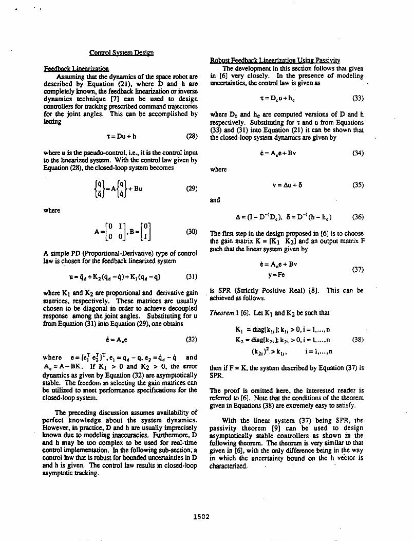
Assuming that the dynamics of the space robot are described by Equation (21). where D and h are completely known, the feedback linearization or inverse dynamics technique (7) can be used to design controllers for tracking prescribed command trajectories for the joint angles. This can be accomplished by

%=Du+h (28)

lccting

where u is the pseudo-mntrol. i.e., it is the control input to the linearized system. With the control law given by Equation (28), the closed-loop system becomes

where

0 1 A=[0 o]*B=[;]

A simple PD (Roportional-Derivative) type of control law is chosen for the feedback linearized system

u = qd+K2(4d -q)+Kl(qd -9) (31)

where K1 and K2 are proportional and daivative gain matrices, respectively. These matrices are usually chosen to be diagonal in order to achieve decoupled response among the joint angles. Substituting for u from Equation (3 1) into Equation (29). one obtains

.

where e=(e, T e,) T T , e ,=qd-q ,e ,=q , -q and A,=A-BK. If K1 > 0 and K2 > 0, the error dynamics as given by Equation (32) are asymptotically stable. The freedom in selecting the gain matrices can be utilized to meet performance specifications for the closed-loop system.

The preceding discussion assumes availability of perfect knowledge about the system dynamics. However, in practice, D and h arc usually imprecisely known due 10 modeling inaccuracies. Furthermore, D and h may bt too complex to be used for d - t i m e control implementation. In the following subsection; a control law that is robust for bounded uncertainties in D and h is given. The control law results in closed-loop asymptotic tracking.

The development in this section follows that given in [a] very closely. In the presence of modeling uncatainties. the control law is given as f .

‘t=D,u+h, (33)

where Dc and hc an computed versions of D and h respectively. Substituting for ‘t and u from Equations (33) and (31) into Equation (21) it can be shown that the closed-loop system dynamics are given by

e=A,e+Bv (34)

where

v=Au+6 (35)

and

Ihe first step in the design proposed in [a] is to choose the gain matrix K = w1 Kz] and an output matrix F such that the linear system given by

i = Ace+ Bv y=Fe (37)

is SPR (Strictly Positive Real) [81. This can be achieved as follows.

Theorem 1 [a]. Ltt K1 and K2 be such that

Kl = diag[kli]; k,i > 0, i = 1 ,..., n K 2 = diag[k,,]; kZi > 0. i = 1. .... n

i = 1, ..., n (38)

(kzj 12.> kli

then if F = K, the system described by Equation (37) is SPR.

The proof is omitted here, the interested reader is xeferred to [6]. Note that the conditions of the theorem given in Equations (38) are extremely easy to satisfy.

With the linear system (37) being SPR, the passivity theorem [9] can be used to design asymptotically stable controllers as shown in the following theorem. The theorem is very similar to that given in [a], with the only difference being in +e way in which the uncertainty bound on the h vector is charactew.

1502

Theorem 2. Let the following two inequalities hold

(39) 1 r

D<-I (r>O)

lD-'(h - hc)k 5 '&I, + d VT >O (c20,drO) (40)

L

Furthennore, let qd E L2. Then if Dc = aI where

(41) C S 1 a>-

r

the closed-loop system is asymptotically stable.

Proof. The closed-loop system as given by Equation (34) can be represented in block diagram fonn 8s shown in Figure 2. It is first shown that the nonlinear block in the feedback path is passive [9].

+ iid Figure 2. Robust Feedback Linearidon Using

Consider

Passivity Theorem.

T I = j-uTvdt (T > 0)

= I-u'(Au + 6)dt

0

T

0

= (-I uTAudt) + (-I ..&It) (42)

Let the first and second integrals on the right hand side be denoted by 11 and 12 respectively. Then

T

0 I, = u ~ ( ~ D " - 1)udt (43)

Noting that

me can obtain

(45)

On the other hand,

Hence

It can be shown that if (ar - c - 1) > 0, then

Hence

T I-uTvdt2- d2 VT>O (49) 4(= - c - 1) 0

Thus a sufficient condition for the nonlinear block to be passive is that a > (c + 1)h.

Additionally, the transfer function of the feedforward block [Ac, B. K] is proper and has no poles on the imaginary axis. Hence it has finite gain [lo]. Since qd E L', then using the passivity theorem P I , one can conclude that the signals u, Ke, and v are bounded. Moreover, since the feedforward block is SPR. Ke(t) = K,e,(t) + K2+(t) goes to zero asymptotically. This in turn implies that el (t) and e#) individually approach zero asymptotically [81.

The first condition of the theorem, given by Equation (39), is easy to satisfy since D is upper bounded. However, the second condition, given by Equation (40). might not be easy to verify in a straightforward manner in all applications.

As an example, nSults arc illustrated for a single link space robot shown in Figure 3. Equation (21) describes the dynamics of this one degree of freedom system. The system inertia, computed using Equation (lo), turns out to be

1503

(54) d = m'(P: + P: + 2P,Plcl) + I, + 1,

(51) jb=-[-p1cv1 m' +;{m+;(~,c, 1 +P,)+IJ- and m ' r moml / (mo + m,). Using Equations (22) and (23). h is dttermined to be

m0

(PlC,, + POCV)]Q1

MY meter) meter) m6g) 1 h . d : - O(Base) 3.0 5.0 30.0 1 (Link) 3.0 6.0 1 .o 3.0

In Equations (50) through (52). c1 = w q , )*% = W q , ) .

Figure 3. A Single Link Pianat Space Robot.

It can bc sfcn tasily that as mg + -,and + -,

D + m,P: + I], h + 0 (53)

Where

Finally, the base attitude dynamics is obtained using Equation (26)

(56) 1 d

\ir = --[mT,(P,cl + PJ + I, Jql

1 - = ~ ' P : + I , r

which lcptsents the case of a fnad base manipulator. Equation (25) is used to dcrermint the evolution of the basc position with time . . (57)

a in Theorem 2 is assumed to be 1.1h for both cases involving uncertainty. The choice of however, is different for the two cases. In the fist case, the

1504

following sixnpliscation to b is used for computing the closed-loop control

The second case corresponds to an even greater simplification to h

1

h, = m’P,P,q, (59)

Figurts 4 through 7 show closed-loop nsults for the nominal case and for the f i t case involving uncertainty. c E 0.01 was choscn to satisfy condition (41) of Theorem 2. d was choscn to be 2.5. Figure 4 shows that asymptotic uacking in tbe pint angle is

Time (seconds)

Figure 4. Joint and Bast Angle Rcsponsts for the Nominal Case and the First Case Involving Uacatainty.

Time (seconds)

Figure 5. Joint Torque Input for the Nominal cast and the First Case Involving Uncertainty.

achieved in the face of uncertainty. This is associated‘ with a slight performance &gadation in the p in t angle response in the sulsc that it has an overshoot. Figure 5 shows that higher magnitudes of joint torque arc required for the case involving uncertainty. Figures4 and 6 show that the base moves in reaction to link motion; this is due to the canservluj~n of linear and angular momentum as discussed previously. However, the joint angle still achieves the right commanded value. Figure 7 shows that the choice of c and d used in this case satisfies condition (40) of Theorem 2.

Time (seconds)

- Figure 6. Motion of the Base Centcr of Mass for the

Nominal Casc and the First Casc Involving Unccxtainty.

Time (seconds)

Figures 8 through 11 show closed-loop results for the nominal case and the second case involving uncertainty. For the second m e , c and d are chosen to

1505

be c = 0.01 and d = 5.0. Trends similar to the previous case axe noticed here also. However, since the extent of mctrtainty is greater. there is more deviation in the nsp0nse.s as compared to the previous case. This is obmed in Figures 8 through 10. Figure 11 confirms that the choice of c and d satisfies the requirements of ’Ibeortm 2.

E cn

i

Y

$

.g

H

h

: Nominal, -- : Uncertainty 0.4 I 1 ,

: Nominal, -- : Uncertainty 1.5 1 1 I

1 1 I I

5 10 15 20 -0.4 ’ 0

Time (seconds)

Figure 10.Motion of the Base Center of Mass for the Nominal Case and the Second Case Involving Uncertainty.

Time (seconds)

Figure 8. Joint and Base Angle Responses for the Nominal Case and the Second Case Involving Uncertainty.

0 5 10 15 20 Time (seconds)

Figure 9. Joint Torque Input for the Nominal Case and the Second Case Involving Uncertainty.

s

A control method based on feedback linearization and passivity concepts that was proposed earlier for fix& base robots is modiried and extended to the case of free base robots. The control law results in

5 10 15 20 Time (seconds)

Figure 11. ’Ihe Quantity c ~ u ~ , + d - ID-’(h - hc)iT for the Second Case Involving Uncertainty.

asymptotic joint angle tracking in the face of bounded uncertainties. For the fmt time, closed-loop simulation nsults are presented using this control method. For the simple example illustrated in the paper, the control method shows promising results.

References

[l]. E. Papadopoulos and S. Dubowsky, “On the Nature of Control Algorithms for Space Manipulators,” Proceedings of the 1990 IEEE International Conference on Robotics and Automation, Cincinnati, Ohio, pp. 1102-1 108.

1506

.. ’ ,

121.2. Vafa and S. Dubowsky, T h e Kinematics and Dynamics of Space Manipulators: The Virtual Manipulator Approach,” The international Journal of Robotics Research, Raleigh, 9(4), August 1990.

131. H. L. Alexander and R.H. Cannon, “Experiments on the Control of a Satellite Manipulator,” Proceedings of the 1987 American Control Conference, Minneapolis, Minnesota.

141. Y. Umetani and K. Yoshida, “Continuous Path Conuol of Space Manipulators Mounted on OMV,”

[SI. Y. Masutani, F. Miyazaki, and S. Arimoto, “Sensory Feedback Control For Space Manipulators,” Proceedings of the 1989 EEE international Conference on Robotics and Automation, Scottsdale, Arizona.

c

Acta Astro~uti~a, 15(12), 1987, p ~ . 981- 986.

[a]. C. Abdallah and R. Jordan, “A Positive-Real Design for Robotic Manipulators,” Proceedings of the 1990 American Control Conference, San Diego, California, pp. 99 1-992.

[7]. M. W. Spong and M. Vidyasagar, Robot Dynamics and Conml, John Wiley, New York, 1989.

[81. J-J. E. Slotine and W. Li, Applied Nonlinear Control, Prentice Hall, New Jersey, 1991, pp, 127,399.

[91. C. A. Desoer and M. Vidyasagar, Feedback Systems: input-Output Properties, Academic Press, New York, 1975, pp. 173-186.

[lo]. J. C. Doyle, B. A. Francis, and A. R. Tannenbaum, Feedback Control Theory, Macmillan, New York, 1992, pp. 16.

1507

AIAA-94-3654-CP

NONLINEAR CONTROL OF SPACE MANIPULATORS WITH MODEL UNCERTAINTY

Manoj Mittal* and C. -H. Chuangf School of Aerospace Engineering Georgia Institute of Technology

Atlanta, Georgia 30332-0150

. and

Jer-Nan Juangs Spacecraft Dynamics Branch

NASA Langley Research Centa Hampton, Virginia

Abstract For robotic manipulators, nonlinear control using

feedback linearization n invase dynamics yields good results in the absence of modeling uncertainty. Howeva, modeling uncertainties such as unknown joint friction coefficients can give rise to undesirable characteristics when these control systems are implunented. In this work, it is shown how passivity concepts can be used to supplement the feedback lineariZation control design technique, in order to make it robust with respect to bounded uncertain effects. Results are obtained for space manipulators with freely floating base; however, they arc applicable to frxed tmsc manipulators as well. The controller guarantees asymptotic tracking of the joint states. Closed-loop simulation rtmlts are illustrated for a planar single link space manipulator.

1. Inwductibn The dynamics of space manipulators differs from

that of fixed base manipulators since their base is frec to move. The base could be either a spacecraft or a satellite. The movement of manipulator arms produces reaction forces and torques on the bast. Therefore the resulting motion of the base has to be accounted for in the dynamic modeling of the manipulator. Howeva, Papadopoulos and Dubowsky1 showed that a dynamic model for space manipulators with a frec base is similar in smcture 10 the dynamic model for fixed base manipulators. An obvious similarity is that rhe inUtia m e in tach case is symmetric and positive definite. In fact, the dynamic model for fixed base manipulators can be viewed as a subset of the model for space Moipulators. In the past, a great deal of attention has been paid by researchers in the area of dynamic modeling of space manipulators. Some interesting

notions have emcrgcd from modeling studies, of significant importance among which is the idea of virtual manipulators2. On the other hand, little effort has been ma& in the 8rea of robust tracking control law synthesis for space manipulators. A few concepts have been praposed for joint trajectory control and inertial end tip motion control of space manipuIators. Alexander and Cannon3 showed that the end tip of a space robot can be controlled by solving the inverse dynamics that includes motion of the base. Their method assumes the mass of the spacecraft to be relatively large compared to that of the manipulator it carries, and also requires much computational effort to determine the control input. Note that some future rpacc systems are expected to have the manipulator and spacecraft masses of the same order. Yoshida and Umetani4 proposed the generalized Jacobian matrix that relates the cad tip velocities to the joint velocities by taking into rmunt the motion of the base. However, robustness of the control scheme with respect to

A nonlinear controller based on feedback linearization and passivity concepts was developed by Chuang, Miaal, and hang5. The feedback linearization technique for nonlinear control system design has been generally accepted to yield good results. However, these type of controllers require full inversion of the nonlinear system model in real-time. This computational imposition can restrict and limit the applicability of the technique. In Ref. 5. it was shown that if simplifications to the nonlinear model are made in a manncz such that the passivity of the closed-loop system is preserved in a cmain sense, the feedback linearization technique retains it's asymptotic stabilization propatjes.

In this paper, a nonlinear dynamic madcl for space manipulators with uncontrolled base is first, derived.

modeling uncertainties was notaddrd .

Poudoctonl Fellow, AUA Member. Arrirtmt hfcrror, AIAA Senior Munkr.

'bpyrigh~ 01994 by the Institute of Amnrutia md AstmuutiU. All rights recaved."

0

t * Rincipd Scientist, AlAA Fellow

1009

The development of the expressions for linur and angular momenta of the system closely follows that givar in Re€. 6; bowtver, the fam of the finnl equations of motion is diffaent It is then shown how passivity concqts un be& in amjunctim with the feedback linuriution technique to design robust aonlinw controllers f a space manipulators. The proposed amtrol scheme can be used for f i x 4 base manipulators also. Tbe control scheme uses i n v m e dynamics; boweva, it is robust in the face of bounded modcling rmceruinties which might Uist due to 8 number of factors including impropw friction modeling. The

p i n t angle uajectories whose rccehtion is bounded in tonmlla 8symptotically tracks prescribed time vuying

thCL2Irpace.

2. & S Y s m

BlseFrame

f f

End A Tip

4 Fig. 1. A Space Robot.

'Ihe bevelopmau of 8 nonlinear dynamic modcl for a rpece manipuktor yscun whoscboe is rmconoolled is discussed in this Section. A t p c e manipulator tystem in a satellite orbit can be approximately considered to be floating in 8 aon-gnviutional environment As shown in Figure 1, the manipulator and the base can be mledrs 8 set of n+l rigid bodies connected through n pints. Tbe bodies IVC numbcred

from zero to n with the hasc king Oand the end tip being n. Each p i n t is then numbued accordingly from a~ to n. "he angular displacemenu of the joints can be repreoented by rjoint vector,

The mass and inertia tensor of the i* body ut denod by mi md Ii; md the kr th ttnsoI is expressed in terms d the base h e wordinates.

.

2 1 A worUte frame fued lo the orbit of the satellite

a n k d d e r e d to bean matial -e, denoted by G. In addition to XI, mother coordinate frame f g is &fined that is aaached to the base with its origin Aocated at the base ccnter of mass. The attitude of the bese itself is given by roll, pitch, and yaw angles. In the aquel, dl vectors u c expressed in the base fixed coordinate ues.

Lu Ri and ri k b e position =tors of the center of mass of the i* link with respect to frames a and ZB, rcsptctively. Then

when RB is the position vector from the origin of the h e Z~to the b s e ccnter of mass. Let Viand ni be the linear and angular velocities of the ctnm of mass of tk ;*link with resptcttoframe Z1 and Vi and %be the linur and angular velocities of the same point with respact to frame &. Then Vi m d n i Can be WitM Bs

(3) a1 'RB +o, (4)

V, = V, +vi +R, x ti

VB and RB lrrc the linear and angular velocities of the base mtu of mass with respect to frame XI. Note rhat for my r p a ~ e manipulator, Vi and for each link c ~ n bc rcptsentcd by the following forms

1010

22- The linear momentum P and the angular

momentum L of the whole system are defined as follows

L= + miRi xV,] i=o

Substituting Equations (2) through (8) into Equations (9) and (10) yields

where

H, = mc13x3, H, E RJx3 H a = - mc[rc x], Hvn E R3x3

H, = Emir,, H, E R"'

(13) (14)

(15) i l

For any vector f =[fl f2 f3f , (f x] is defined as 0 -fj f,

Since the working environment is non-gravitational m d no actuators generating external forces are employed, the linear and angular momenta of the whole system are consmed. Since the inertial frame is fixed to the orbit, the entire system can be assumed to be

otatc. Thus the above two momenta are always z m for the system. Note that it is implicitly implied that the mtellite is a non-spinning body. By using the fact that the linear end angular momenta are zcfo, Equations (1 1)

donary with respect to the inertial frame at the initial

nd (12) nsult in

23

written as The total kinetic energy of the space robot can be

Using Equations (3) through (8) and (1 3) through (1 7) the kinetic energy can be expressed as

where Hq is the inertia matrix corresponding to the b e d base manipulator

H, = $[miJf t JL+J~I iJ~] , Hq E R""" (22) I l l

Equation (21) for thc system kinetic energy can be simplified as follows. Substituting for VB from Equation (1 8) leads to

I 1 T=5@4flB + ~XZJ + -qfWq 2 (23)

Further, substituting for RB from Equation (19). one obtains an expression for the system kinetic energy .solely in t a m s of the joint variables.

I 2 (27) T = -q'D(q)q, DE REX'

when D is the inertia matrix of the system and is given bY

It can be shown that D = DT > 0. It is interesting to note that the system inertia matrix obtained in Reference [I] is of the same form as above. However,

. ( 1 ‘ *

the expressions for W, M, md Z matrices rre dif€amt ’2his is because a diffaent approach, vir, the corrccpt of barycenters, is ased in the model derivation of Reference [l]. It is also noteworthy that the inertia matrix obtained above requires only a 3 x 3 matrix inversion, while that obtained by Masutani, Miyazaki, awl Arimod rcquiresa6x imatrix inversion.

Since there is no potential energy in non- gravitational environmengthe Lagrangian A, is qual to thekineticenergy

A = T (29)

So the system dynamics is given by

matrix consisting of viscous friction coefficients for the manipulatot pints. The vector sgn(q} is defined in a component-wise sense. It turns out that in many manipulator pints, friction also displays 8 dependence on joint position. However, such effects are not eonsidered hen. Then ut other effects like bending effects that m difficult to model and also neglecttd in tbe pnsent model.

Joint Friction Torque Vixolrs

Friction Sratic coulomb’s Friction

Kinetic Coulomb’s Friction

where t i s the a x 1 vector of pint torques. The equation of motion for space manipulators is then obtained by using Equation (30).

Paralleling thc development for fixed base robots given by Spong and Vidyasagar7, the elements of the mauix C are obtained as

yzqwcsau the pint torque vector due 10 friction. As pointed out by CLaig*. the total friction at each pint can be regarded as the sum of Coulomb friction and Viocous friction. Coulomb friction is constant except for 8 dgn dependence on the pint velocity. Viscous fiction, in general, depends on various powers of joint velocity. However, higher powas contribute Signifcantly only at high pint velocities. Manipulam usually do not stain such high velocities. Therefore, it is sufficient to consider only the linear dependence of viscous friction on joint velocity. Figure 2 shows 1 friction model consisting of Coulomb friction and linear viscous friction. Using this model, the joint friction torque =tar CanbC~PreSentCdaS

t f - wn{il)+ril (9)

where X is 8 diagonal matrix consisting of Coulomb friction constants for the pints, and r is a diagonal

Fig. 2. Joint Fiiction Modcl Consisting of Coulomb’s Friction and Linear Viscous Friction.

2.4 The translational vclocity of the base center of

mass can be written in m s of joint velocities by using the expression for f l ~ from Equation (19) in Equation (18).

V, = - H,’ [ H, - H&-’Z]q (35)

Also, tk bast angular velocity &om Equation (1 9) is

Using the above expressions, the evolution of the base position and orientation with time can be determined.

3.

Assuming that the dynamics of the space manipulator is &Scribed by Equation (31), when D and h arc completely hrown, the feedback linearization or inverse dynamics7 technique can be used to design controllers for tracking prescribed command mjectories for the pint angles. This a n k accomplished as outlined in the following subsection.

1012

. I I I

1

. . . 3.1

f m . Let the joint torque vector bc of the following

t = D u + h 0 7 )

what u is the pseudo-control, i.e., it is the control input 10 the resulting linearized fistem. With the control law given by Equation (37), the closed-loop system becomes

E]= A[ 81 + Bu

where

0 1 A=[o o]*B=[;] (39)

A simple PD (Proportional-Derivative) type of conml law is chosen for the feedback linearized system

u = qd +K2(4, - 4) + K1 (qd -9) (40)

when K1 and K2 are proportional and daivative gain matrices, respectively. These matrices are usually chosen to be diagonal in order to achieve decoupled response among the joint angles. Substituting for u from Equation (40) into Equation (38). one obtains

i = Ace (41)

w h e r e CE[e:e:JT,et=qd-4,errqd-q. A,=A-BK,and K=[K, K2]. IfK1 >OandK2> 0, the error dynamics as given by Equation (41) is asymptotically stable. The frecdom in selecting the gain matrices can be utilized to meet performance sptcifications for the closed-loop system.

The pnceding discussion assumes availability of perfect knowledge about the nonlinear system dynamics. Howevw, in practice, D and h are usually imprecisely known due to modeling inaccurixies. For instance, the controller would k designed using the best estimates for friction coefficients. ?he actual joint -friction might be different from that which is assumed 'for the controller design. Thus the controller uses computed versions of D and h. ?he objective here is to design a control law that is robust for bounded Vapiations in D and h due to bounded uncatain dynamic effects. This issue of robust control design is discussed in the following subsection, when it will be seen that the control law results in closed-loop asymptotic tracking.

'V' . . . 3.2 2

control law be givur 8s In the presence of modeling uncertainties, let the

t = h l + i i + w (42)

when 6 and i an computed versions of D and h, respectively. The additional feedback w(t) has been introduced to compensate for the modeling uncertainties. Substituting fort and u from Equations (42) and (40) into Equation (31) it can be shown that the closed-loop system dynamics is given by

e= Ace+Bv (43)

and

'Ihe fim step in the proposed design is to choose the gain matrix K = (K, K2] and an output matrix F such that the linear syslem given by

t- A,e+Bv y=Fe

is SPR (Strictly Positive Rcal). 7his can be achieved as outlined in the following ?heorem. A definition of the concept of Strictly Positive Realness can be found in Slotine and Li9.

Tlvprcm 1[10]. Let K1 q d K2 be such that

KI =diag(k,i) kli >O, i = l ,..., n K2 = diag[k2i); kZi > 0. i = 1. .... n (47)

(k2i l2 > k1i 9 i = ll...,n

then if F = IC, the system dcscribcd by Equation (46) is SPR.

Note that the conditions of the Theorem as prescribed by (47) arc extremely easy to satisfy.

With the linear System (46) being SPR, the Passivity -Theorem11 can be used to design asymptotically stable controllers as shown in the

1013

following 'Ibeacm. Tbe notation lxh = (jxTxdt)lll

is used in the nequel. 0

Thrbrnn. suppose-

meta, E L2. (a) The &sired pajcctory for p in t variables is such

(b) Finite $, and Bt exist such drat thc unccmn * tyin h is bounded as follows.

(c) The additional feedback w(t) in the wnm1 law of Equation (42) is of the following form.

w(t)=au(t) ( a z o ) (49)

Unda thesc conditions, if a is chosen such that

a>*(?)

whac el *a&(D). u2=craX(D-b), A-X,,(D); then

&&. The closed-loop system as given by Equation (43) can be represented in block diagram form as shown in Figure 3. It is first shown that the nonlinear block in the feedback path is passivell.

the closed-bop systcm (43) is asymptotically stable.

SPR

v=Au+S

=[I - D"b]u + D"[h - i - w] .. .

(52)

when x I [D - b]u + h - 6 . Substituting for v from Equation (52) into Equation (5 l), the integral becomes

= D"x - D"w

Let the first and second integrals on the right hand side be denoted by 11 and 12 respectively. Then

1

0 -4 = I ufD"x dt

S IuITID"xh (Holder's Inequality) (54)

Note that

1

0 ID-'xC = / X'D-~D-]X dt

f

0 S A,(D-TD-l)j~T~dt (55)

and

Substituting for Am,x(D-TD-l) from (56) into Inequality (55) and then taking the square toot of both rides. one gels

Passive (58)

1 Fig. 3. Robust Feedback Linearization Using -11 ~,l.lrlxh

Passivity Theorem.

Consider -

Recalling that x=[D-fi]u+h-h. and using Schwan's Inquality,

From Equation (44). v is given as follows.

1014

Inquality (59) be expressed d n g Inqualities Thus a sufficient condition for the nmlincar block to be (48) and (60) as

, passiveisthat a>X I X h S (0, + Pi + 82 (61)

Additionally, it is observed that the transfer

les on the imaginary axis. Hence it has

11 ~ - - [ ( o Z + B ~ ) I U P : + B ~ ~ U R ] (a) m m ad E L2,ttren-ghemivitykXm11, one can conclude that the signaIs u, Ke, and v are bounded. Moreover, since the feedforward block is SPR, Ke(t) = K,el(t) + IC2+([) goes to zero

individually approach zero asymptotically*.

bound for 11 is obtained in the following form. using mualiv (''1 in Inequality (58)* a lower

fUnctian of the f#dforward block [&, B, K] pro^ and has no 6nitc gain* !O . since according to kumption (a) of the 1

"I

Now consider

T m~ympt~t idy. This in turn implies that e1 ( I ) and %(t) 1, = uTD"w dt

0 T

0 = a/ufD"udt

2 aX,, (D-')j uTu dt T

0 (63)

Noting that

an upper bound for I2 is obtained as follows.

nus, using Inqualities (62) and (65) in Equation (53),

It can k shown that if [ ~ - ~ ) > o , t h e n

Remark. (i) Some of the methods proposed in the past for designing robust con0ol)en for robotics problems result in introduction of chattering in the ~ ~ n t r o i f . When the design method is modified to make the conwl smooth. closed-loop asymptotic tracking is generally compromised to some extent, In the control design proposed by 'Ihcam 2, the achievement of robustness can be qualitatively understood as follows. The control law given by Equation (42) comptnsates for the uncertainty due 1~ unknown I) and h by employing additional feedback w. If the choice of w satisfies the assumptions of the Theorem. asymptotic stability for the pint a m states is achieved.

(i) The results of the Theorem are applicable to space manipulators as well as fixed base manipulators. Finally, it should be noted that the control design suggested using the results of the Theorem is not unique. First of all, w(t) need not be restricted to be of the form given by Equation (49) and second, even within Lhc scopc of the suggested design, there is a considerable amount of margin for performance optimization.

4.

7" results of qplying Theonms 1 and 2 in order to llchieve a robust cbnuol design are illustrated for a planar sin le link space manipuhor. Figure 4 shows

A nonlineaf dynamic model for thc robot is obtained using the results of Section 2. Equation (31) describes the dynamics of this onc degree of M o m system. The

(67) ( a 2 /a1

f ( i u ~ 2 -,+j -- such a panar d one link space robot. which in turn would imply

1015

where

O(Base) 3.0 - 5.0 30.0 1 (Link) 3.0 6 .O 1 .o 3.0 .

End Tip

I

Fig. 4. A Single Link Planar Space Robot.

Using Equations (32) through (34). h is found to k

w h e n x and y are respectively the coefficients of Coulomb and viscous friction. In Equations (70) through (73) mol I moml /me, m, = mo + m,, ~1 m C&q1). and t i Sh(q, )

which represents the case of a fixed base manipulator. E q h o n (35) is used to determine the evolution of the base position with time

where Sin& + ql), cv! CONY + ql) . Finally, the base attitude dynamics is obtained using Equation (36):

Assuming that no modeling uncertainty exists, a foulback linearizing conmller is designed for the one link space manipulator using the control law given by Equation (37). Simulation is carried out using automatic step size second and third order Runge- Kutta-Fehlberg integration methods13. Table I lists physical parameters of the example robot used in the simulation. Note that the base and link masses are rssumcd to be of the same order of magnitude. The values of Coulomb and viscous friction coefficients are mkcatobe

Next, it is rssumcd that the value of the Coulomb

(78)

M o n aefficient, x is unknown, but that

0.5 S x 5 0.75

Since uncertainty exists in the h vector, the computed version of h is given by

1

h = hL+i 09)

where = 0.5, which is the nominal value of the Coulomb friction coefficient. The response of the controller with x = 0.75 and without any additional

1016

feedback is shown i n F i p 6 . It canbclcenrhat thae is a steady-state csrot m the pint mgle response. The steady-state a m in this particular instance can be eliminated by adding an integral fecdback term to the control law given by Equation (40); however, this is accompanied by 8 large overshoot. Hence, a need exists for making the control law robust with respect to the uncertainty. The nsults of Theorem 2 arc used for the design. It is fm notid that

Response Without Uncertainty 1

0.8 - 0.6 -

Time (seconds)

5. Joint Angle Response With No Modeling UnCatainty.

Clearly, l h - i l T is maximum when b-iI is maximum. Hence the controller is designed for x = 0.75, and it works far all other values of x lying in the range indicated by (78). The design involves determining a suitable value of a that satisfies Inquality (SO), assuming that finite B1 and 82 exist for the bound given by Inquality (48). Figure 7 shows the variation of system inatia. D, given by Equation (69), with respect to the pint angle. From this plot, it is easily found that X = 10.2273, and 01 = 5.3571. Clearly, by defmition, 02 = 0. Hence the requirement (SO) of Theorem 2 translates to:

a > l.W(B,) (81)

'Ihe wluw of and B2 are obtained in & iterative manner. Starting with an assumed set of values for these parameters, closed-loop simulation is paformed with the resulting value of a as obtained by Condition (81). If the pint crrur states are not asymptotically

stable. dris implies that Inquality (48) must have been violated. The amount by which violation occurs is used as a measure to update the estimates of 81 and 82. ?he process is rcpeated until convergence is obtained. For the present example. it yas found that = 12.5 and p2 = 1.5 satisfy Inquality (48). This resulted in a choice of a = 25.0 for the design. Note that the process implicitly assumes at the outset that condition (b) of Theorem 2 will hold.

:Robust Control, -:Nominal Control

0.6

0 5 10 15 20 Time (seconds)

6. Joint Angle Response With Bounded UaCertainty in Friction Modeling.

l2 g

-4 -2 0 2 4 Joint Angle (rad)

Fig, 7. Variation of System Inertia Matr ix With the Joint Angle.

Figures 6 md Figures 8 through 12 show the ciasbd-loap mponscs for the design, with and without the inclusion of additional feedback. Figure 6 shows drat asymptotic =king in the pint angle is achieved in the face of uncertainty. Figures 9 and IO show b a t the bese moves m reaction to link motion; this is due to the conscrvation of linear and angular momenta as discussed in Section 2. Figure 11 depicts the

1017

a . I 4

:Robust Control, -:Nominal Control 0.4 t- i

0 5 10 15 20 Time (seconds)

Fig. 8.

0 n

-0.1 8 E! ‘f!

-0.2 3 cp

Joint Velocity Response With Bounded Uncertainty in Friction Modeling.

,:Robust Control, -:Nominal Control

-0.3 0 5 10 15 20

Time (seconds)

Fig. 9. Base Attitude Response With Bounded Uncatainty in Friction Modeling.

:Robust Control, --:Nominal Control 0.2 r n E Y

Y.2’ 0 5 10 15 20

Time (seconds)

Fig. 10. Base Position Response With Bounded UncCnainty in Friction Modeling.

0 5 10 15 20 Time (seconds)

Fig. 11. The Quantity f$luiT + Bz -1h - ill, With

:Robust Control, --:Nominal Control Bounded Uncertainty in Friction Modeling.

10

5

- 0 0 5 10 15 20

Time (seconds)

Fig. 12.Joint Torque Input With Bounded Unccnainty in Friction Modeling.

satisfaction of Inequality (48). Figure 12 shows the pint torque input requirements. It was confmed though simulations that the controlla designed works well for any value of 2 within the range indicated by (78). Indeed for my value of x < 0.75, the uncenainty bound on h is wisfied by a greater margin.

5.

A nonlinear dynamic model was obtained for space manipulators with uncontrolled base. A robust control method based on feedback linpabtion and passivity concepts was proposed for space manipulators. The method is applicable to fixed base manipulators as well. The convol law results in asymptotic joint angle tracking in thc face of bounded uncertainties such as those due to imprecise friction modeling.

1018

Rererences

E. Papadopoulos and S. Dubowsky, "on the Nature of Control Algorithms for Space Manipulators," Proceedings of the IEEE International Conference on Robotics and Automation, Cincinnati, Ohio, May 1990, pp. 1102-1108. c 2 Vafa and S. Dubowsky, "The Kinematics and Dynamics of Space Manipulators: The Virtual Manipulator Approach," The Infernational Jownal of Robotics Research, Vol. 9, No. 4,

H. L. Alexanda and R.H. Cannon, "Expaiments on the Control of a Satellite Manipulator," Proceedings of the American Control Conference, Minneapolis, Minnesota, June 1987. K. Yoshida and Y. Umctani, "Control of Space Manipulators with Generalized Jacobian Matrix," in Space Robotics: Dynamics and Control, Eds. Y . Xu and T. Kanade, Kluwer Academic Publishers, Boston, Massachusetts,

C. -H. Chuang, M. Mittal, and J. -N. Juang, Tassivity Based Robust Control of Space Manipulators," Proceedings of the A I M Guidance, Navigation, and Control Confmncc, Monturey, Califarnia, August 1993. Y. Masutani, F. Miyazaki, and S. Arimoto, "Sensory Feedback Control For Space Manipulators," Procetdings of the 1989 IEEE International Conference on Robotics and Automation, Scortsdak, Mzona, M a y 1989, pp. 1346- 135 1. M. W. Spong and M. Vidyasngar, Robot Dynamics Md Control, John Wiley, New Yak, 1989. J. J. Craig, introduction to Robotics Mechanics and Control, Second Edition, Addison-Wesley,

J-J. E. Slotine and W. Li, Applied Nonlinear Control, Rntice Hall, New Jersey, 1991, pp. 127,399. C. Abdallah and R. Jordan, "A Positivc-Real Design for Robotic Manipulators," Proceedings of the 1990 American Control Conference, San Diego, California, M a y 1990, pp. 991-992. C. A. Dcsoer and M. Vidyasagar, Feedback Sysrems: lnpur-Outpuf Properties, Academic

J. C. Doyle, B. A. Francis, md A. R. Tanncnbaum, Feedback Control Theory, Mcmillan, New Yark, 1992, pp. 16. MATLAB Reference Guide, n t e Mathworks

August 1990. p ~ . 3-21.

1993, p ~ . 165-204.

1989, p ~ . 214-215.

RSS, NCW Y e , 1975, p ~ . 173-186.

hc.. A u W 1992. DD. 351-353.

1019