7 O ADGAR9 089 COLD REGIONS RESEARCH AND ENGINEERING LA B HANOVER NH F/G A/12I NVESTGAT NS OF SEA ICE ANISOTROPY, ELECTROMAGNETIC PROPERTIE--ETCL

SEP So A KOVACS, R M MOREY

~MI1

_ Ail~momo

REPORT 80-20

Investigations of sea ice anisotropy,electromagnetic properties, strength, andunder-ice current orientation

DTICjftELCTEC

~77

L

Cover: Example of A Ice crystal structure and related'oitag amplitude anisotropy as determlned byriwdo echo sounding measurements The lighttoned speckling In the photograph shows wherebrine pockets are situated betwen the 1-mm-wide ice platelets that compose an Ice crystal.Individual ice crystals are quite irregular andare represented In this thin section by differentshades of gray. Thin section diameter -7.5 cm.

i "A

I

! CRR1EL -- 2

iI

jnvestgations of sea ice_ nisotropy, -electromagneticproperties, strength, andjunder-ice current orientation

Austin/Kovacs a Rexford M. 4orey/

Sep~

Prepared forOFFICE OF NAVAL RESEARCHandNATIONAL OCEANIC AND ATMOSPHERIC ADMINISTRATIONBy

UNITED STATES ARMYCORPS OF ENGINEERS

.Z " COLD REGIONS RESEARCH AND ENGINEERING LABORATORYHANOVER, NEW HAMPSHIRE, U.S.A.

ApmW for public release; disirtuion unlimited ~? /~-S-

SECURITV CLASSIFICATION OF THIS PAGE (When Data 800eme)________________

REPORT DOCUMENTATION PAGE RRA MBT P0W-REPOR UM-uER 7 GOVT ACCESSION NO: S. RIECIPIENT'S CATALOG NUMSESR

CRREL Report 80-20 ,~ -~/~ ~~ _ _ _ _ _ _ _

14. TITLE find S"dihl) S. TYPE Of REPORT & PEF4OD COVERED

INVESTIGATIONS OF SEA ICE AN ISOTROPY, ELECTROMAGNETICPROPERTIES, STRENGTH, AND UNDER-ICE CURRENTORIENTATION S. PERFORMING ORG. REPORT NUMBER

?7. AUTHONWe 8. CONTRACT OR GRANT NUMNEWa.)

ONR Project NR 307-393Austin Kovacs and Rexford M. Morey NOAA R.D. No. RK4180065

S. PERFORMING ORGANIZATION NAKE AND ADDRESS /10. PROGRAM KLEMJA PROJECT. TASK

U.S. Army Cold Regions Research and Engirneering Laboratory AE OK NT"ma

Hanover, New Hampshire 03755

11. CONTROLLING OFFICE NAME AND ADDRESS 12. REPORT DATE

U.S. Navy, Office of Naval Research September 1980and 12. HNMER OF PAGESU.S. Dept. of Commerce, National Oceanic & Atmospheric Administratio 23

14. MONITORING AGENCY NAME A A00DRESS11(ft WftumI bm CenfrOlfl Office) IS. SECURITY CLASS. (of #do a weft)

Unclassified

a. DECLASSIFICATION/DOWNGRADINGSCHIEDUL

16. DISTRIBUTION STATEMENT (of Ws. Repart)

Approved for public release; distribution unlimited.

17. DISTRIUUTION STATEMENT (of t0 abaft aWII In Black 20. If difeamt horn Rapfit

IS. SUPPLEMENTARY NOTES

is. KEY WORDS (CanthuaeM -V0 'ovm. ait neoearn ad 1denti by wee.k nunw)

Anisotropy, Strength (mechanics)

composed of an array of lossy parallel plate wavegu Ides. The fundametal relation between the average bulk brinevolume of sea ice and its electrical and strength properties Is discuseed as Is the remote detection of under-ice currentalignment. It was found that 1) the average effective bulk dielectric constant Is dependent upon the average bulk brinevolume of the sea Ice; 2) sea ice anisotropy, arising from a bottom structure of crystal platelets with a preferred c-axishorizontal alignment, can be detected by radio echo sounding measurements made not only on the ice surface but alsofrom an airborne platform; 3) the effective coefficient of reflection from the sea ice bottom decreases with increasingaverage effective bulk dielecjic constant of the ice, decreases, with increasing bulk brine volume, and Is typically one tol

PD ~ 103 M~m. O ~ MW 511 SSOETEUnclassmfed

SEDIIRITY CLA1S1FICATIOR OF ThISPA"1ME m, OeRAtet

W pNT CLMIA0 FT" " ~a@SIO

11. Controlling Office Name and Address (cont'd)

Arlington, VA 20390 Fairbanks, AK 99701

20. Abstract (cont'd).

two orders of magnitude lower dhan the coefficient of reflection from the ice surface; and 4) the losses In seaiceIncrease with Increasing average bulk brine wluime.

ii UnclassifiedWCUINTY CLASUPICATFON Of TwaS PA@SfW#Mu Deft bi...

PREFACE

This report was prepared by Austin Kovacs, Research Civil Engineer, Applied Research Branch,Experimental Engineering Division, U.S. Army Cold Regions Research and Engineering Laboratory,and Rexford M. Morey, Morey Research Company, Nashua, New Hampshire (CRREL Expert).

This study was supported by the Office of Naval Research, Project NR 307-393, and in part bythe Bureau of Land Management, through interagency agreement with the National Oceanic andAtmospheric Administration under the Alaska Outer Continental Shelf Environmental AssessmentProgram. The helpful comments of Dr. Wilford F. Weeks of CRREL on the manuscript areacknowledged.

iN

A .

DIt

iri

L -' ,

1

CONTENTS

PAgeA bstract ................................................................................................................................... iPrefar ..................................................................................................................................... iiiIntroduction ............................................................................................................................. 1Field program ........................................................................................................................... 1Results and discussion .............................................................................................................. SConclusions .............................................................................................................................. 15Literature cited ........................................................................................................................ 16Appendix: Data analysis procedures ........................................................................................ 17

ILLUSTRATIONS

Figure1. Map of 1977-1979 impulse radar studies ..................................................................... 22. Relative voltage amplitude of reflected wavelet from the snow and ice surfaces, and

the center frequency of the spectrum of the reflected signal from the snow andice surfaces when the antenna was elevated at site WD-79 .................. 6

3. C-axis direction and center frequency of the spectrum of the reflected signal fromthe ice bottom vs antenna E-field azimuth at site WD-79, when the antenna waselevated and when it was resting on the ice surface .............................................. 7

4. C-axis direction and relative voltage amplitude of the wavelet reflected from the icebottom vs antenna E-field azimuth at site WD-79, when the antenna was elevatedand the ice surface was snow-covered and snow-free ............................................. 7

S. C-axis direction and relative voltage amplitude of the wavelet reflected from the icebottom vs antenna E-field azimuth at site WD-79, when the antenna was restingon the ice surface .................................................................................................. 8

6. Configuration of dual antennas mounted to the helicopter during on-ice and airbornesounding of sea ice ............................................................................................... 9

7. C-axis direction and relative voltage amplitude of the wavelet reflected from the icebottom vs antenna E-field azimuth at site WD-79, when the antenna was air-borne, on the ice surface, and mounted to the helicopter approximately 30 cmabove the ice surface ............................................................................................. 10

8. Graphic records of airborne impulse radar echo sounding of sea ice ............................ 109. C-axis direction and relative voltage amplitude of the wavelet reflected from the ice

bottom vs antenna E-field azimuth at site Tig-79 .................................................. 1110. C-axis direction and relative voltage amplitude of the wavelet reflected from the ice

bottom vs antenna E-field azimuth at the Boulder Patch site ............................... 1111. Ice cores obtained at the Boulder Patch site ............................................................... 1112. C-axis direction and relative voltage amplitude of the wavelet reflected from the ice

bottom vs antenna E-field azimuth for when the antenna was "on" the ice andairborne at site G .................................................................................................. 12

13. Brine volume and salinity distribution vs depth at site WD-79 .................. 1314. Average effective bulk dielectric constant vs average bulk brine volume of ice ............ 13

Iv

Figure Pap15. Transmission losses in ice vs its average bulk brine volume ........................................... 1416. Average effective coefficient of reflection from the ice bottom vs average effective

bulk dielectric constant of the ice ........................................................................ 1417. Average effective velocity of the electromagnetic signal in ice vs its average bulk brine

volum e ................................................................................................................... 1418. Schematic for dual-antenna electromagnetic signal flight paths ................................... 15

TABLES

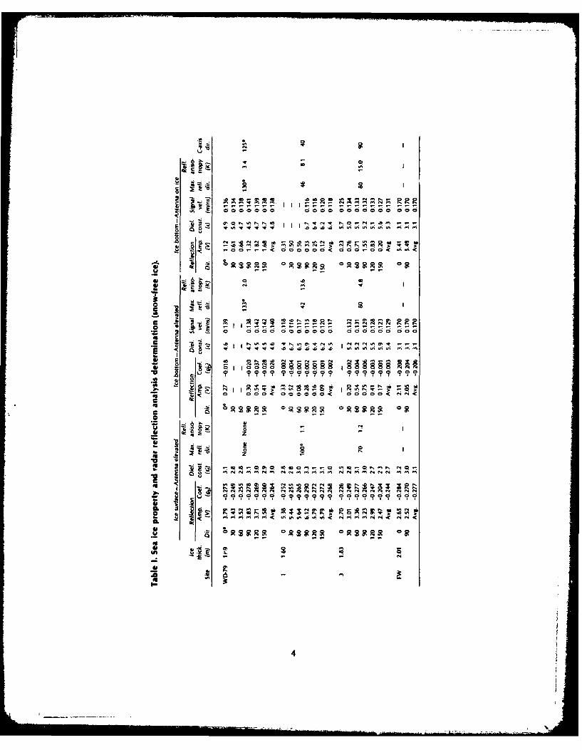
TableI. Sea ice property and radar reflection analysis determination (snow-free ice) ................ 4II. Sea ice property and radar reflection analysis determination (snow-covered ice) ........... 5

Ill. Site average bulk brine volume and minimum effective electromagnetic propagationlosses ................................................................................................................... 5

IV. Site ice thickness, average bulk brine volume and average dielectric constant .............. 13

v

INVESTIGATIONS OF SEA ICE ANISOTROPY,ELECTROMAGNETIC PROPERTIES, STRENGTH, ANDUNDER-ICE CURRENT ORIENTATION

Austin Kovacs and Rexford M. Morey

INTRODUCTION d) the surface of the sea ice had no definite anisotropictrend as determined from EM reflection measurements.

The in situ electromagnetic (EM) properties of sea This paper extends the previous studies on the EMice are important in developing instrumentation for the properties of sea ice as determined with an impulseremote sensing of ice thickness and, indirectly, current radar sounding system operating on the ice surface andorientation at the ice/water interface. Studies using an from an airborne platform, i.e. a helicopter. The fieldimpulse radar sounding system were made in the spring study was made in March 1979, in the area of Prudhoein 1976 and 1977 (Kovacs and Morey 1978) and in Bay, at the sites shown in Figure 1.1978 (Kovacs and Morey 1979a) on the sea ice in thearea of Prudhoe Bay, Alaska. In these studies it wasfound that when the crystal structure at the bottom FIELD PROGRAMof sea ice had a horizontal c-axis with a preferred azi-muthal orientation, this alignment was for all intents During the April 1978 field program, electromagneticand purposes parallel with the short-term (minutes) sounding measurements of sea ice were made using anunder-ice current measurements made at the time. impulse radar sounding system which radiated a time

It was observed that this oriented structure behaved domain wavelet of about 14 ns duration. The centeras an effective polarizer of transverse electromagnetic frequency of the spectrum of the wavelet radiated fromwaves. The resulting effect was shown to reduce or the linearly polarized broadband antenna was abouteliminate the EM signal reflection from the ice bottom 125 MHz, with the -3 db points of the spectrum atwhen the antenna E-field was oriented perpendicular about 75 and 150 MHz. This antenna was used as bothto the preferred c-axis direction of the ice crystal plate- transmitter and receiver. In March 1979, measurementslets. But when the E-field was oriented parallel with were made using linearly polarized antennas with a cen-the preferred crystal c-axis direction a strong signal ter frequercy of the spectrum of the radiated waveletreturn was recorded. of about 280 MHz, with the -3 db points of the spec-

It was also found, in sea ice having a highly ordered trum at about 220 and 350 MHz. One antenna wascrystal structure in which the crystals have a preferred used for transmission and one as a receiver. The radi-horizontal c-axis alignment, that: a) the frequency ated time domain wavelet was about 6 ns in duration.spectrum of the signal reflected from the ice bottom Both antennas were enclosed in one housing; the dis-varied in the horizontal plane, b) the frequency shift tance between the centers of the dipole antennas waswas found to be related to the ice brine volume, c) the about 30 cm.relative change in bulk dielectric constant versus azi- As in previous studies, radar measurements weremuthal angle did not correlate with the coefficient of made with the radar antenna resting on the ice surfaceanisotropy (in other words a travel-time anisotropy and also with the antenna elevated approximately 1.7iws not measured, only a reflecton onisotropy) , and m above the ice surface. In addition, measurements

710 3C, N

Site 3

70045'M

SCurrent

fleaulari S..

Cress 7'30' vi

rs.~

Prudhoe Site 11111

Foggy T\IG.3 70 15 N

Island TONT 10r-7

Mikkalsen13a y

14e 00 147*00

Figure 1. Map of 1977-1979 Impulse radar studies. Sites 1, 2 and Tig were 1977 or 1978 study locatloni Site Gwavsa study location in 1977 1978 and 1979. Sites WD- 79, 8P, Tig 79 and FW were also study locatons In 1-979

2

were made with antennas mounted on the side of a bottom of the ice was again recorded along the sameNOAA (National Oceanic and Atmospheric Adminis- compass headings as when the helicopter was sitting ontration) helicopter. These measurements were made the ice. An ice core obtained at each site was used towith the helicopter resting on the ice surface, during determine, by visual inspection and compass measure-which time the antennas were supported approximately ment, the preferred c-axis azimuth direction at the ice30 cm above the surface, and also while the helicopter bottom.was in flight at an altitude of 10 to 15 m. From x-y plots (see Appendix) of the average of

Radar measurements from the sea ice surface and ten scans, the two-way travel time of the radar signalfrom the helicopter were made at a site about 1 km in the ice and the relative voltage amplitude of the sig-

north of the Prudhoe Bay West Dock (WD-79). At nal reflected at the snow and ice surface and the icethree other sea ice sites sounding measurements were "bottom" were obtained. The effective bulk dielectricmade with the radar mounted on the helicopter, constant e of the sea ice was calculated fromMeasurements were also made on the ice surface of afreshwater lake. At the WD-79 site the measurement =

procedure consisted of marking a 300 increment polar 2Dgrid on the ice surface, making the radar measurements where c = free space electromagnetic signal velocityat each grid azimuth, and obtaining an ice core from D = tape-measured ice thickness minus 5 cmthe center of the grid. Ice core temperature was meas- t = two-way travel time.ured to 0.10C using a thermistor bridge. Measure-ments were made at the 1 -cm and 5-cm depths and at Five centimeters was subtracted from the measuredeach 1 0-cm increment below 5 cm. With the use of a ice thickness because at the impulse radar frequencyconductivity/salinity bridge, the salinity of the ice used in this study the electromagnetic boundary at thewas later determined from the meltwater of the top bottom of growing sea ice has been found to be about1 A cm of the ice surface and each 10-cm section of this distance above the ice/water interface (Campbellthe ice core. Visual observation of the ice core at and Orange 1974), i.e. at or just above the open den-about the 1 -and 1 36-m depths and at the ice bottom dritic ice platelet structure found on the bottom ofrevealed ice crystal structure and c-axis alignment, growing sea ice.Preferred c-axis azimuth orientation was determined The effective wavelet velocity (V,) in the sea icewith the use of a large compass. These determinations was determined from:are believed to be accurate to within I 100. Sea icebrine volume was calculated from the ice core temper- V = 2D- c (2)ature and salinity data. - - .(

Radar measurements were obtained with the radarantenna elevated 1.7 m above the ice surface, on top An analysis of the frequency spectra (see Appendix)of a wooden structure. A 4-m-square metal screen and the relative voltage amplitude of the signal reflectedwas set on the ice or snow surface under the antenna. from the various interfaces provided additional informa-The radiated wavelet reflected from the surface of the tion about the material being sounded and the nature of

screen was recorded on magnetic tape and later used the interfaces. The voltage reflection coefficient of theto provide a known reference reflection. The screen ice surface (ps) was determined by the ratio of the rel-was then removed and the radar reflections from the ative peak-to-peak voltage amplitude of the ice surfacesnow surface and ice bottom were recorded at each and metal screen reflections. The apparent dielectric300 increment on the polar grid. The snow was re- constant (er) of the ice surface was then determinedmoved, and the above sequence of measurements re- from:peated. The antenna was then placed on the ice sur-face and the reflection from the ice bottom recorded, C' = - (3)again at the same 30 grid azimuths. r ' + S

Measurements made with the antennas mounted onthe helicopter were made with the helicopter resting The effective voltage reflection coefficient of theon the ice. The radar reflections from the ice surface ice bottom (Pb) was likewise determined, then cor-and bottom were recorded. Additional readings were rected for the partial reflection of the energy at themade at 300 azimuth increments. This was followed air/ice interface, using:by a series of slow, 10-m altitude flights over the samesite, during which the radar reflection of the top and p = pb(1 -p 2 ) (4)

3

i~* 00000 0000 0000000 c00

Cc

I~0 <~N 0 4.'

- 00

Coco~0 0000000 00 60 0

6a 10 100

0 00000< N 0 0 i0~ 0<

o- m m- " , - >.~ 0 0000 000 000 0000 00

06 <

. I 0

CC

J

Table II. Sea ice property and radar reflection analysis determination (snow-covered ice).

Snow/ice surface -Antenna elevated Ice bottom - Antenna elevatedRell. Rell.

Ice Reflection Diel. Max. aniso- Reflection Diel. Signal Max. aniso. Snowthick. Amp. Coef. cons,. refI. tropy Amp. Coe. const. vel. rell. tropy C-axis thick.

Site (in) Oir. M (as) (a;) dir. 1K) Dir. (VI (@M (c) (n/ns) dk. (K) dir. (cm)

WD-79 1.69 00 3.73 -0.271 3.0 00 0.24 -0.016 4.6 0.13930 3.22 -0.234 2.6 30 - - - -

60 2.96 -0.216 2.4 None None 60 - - - - 1310 2.4 12SO 3.590 3.76 -0.272 3.0 90 0.26 -0.017 4.6 0.137

120 3.33 -0.242 2.7 120 0.45 -0.031 4.5 0.141150 3.12 -0.232 2.6 150 0.38 -0.026 4.6 0.140

Avg. -0.245 2.7 Avg. -0.023 4.6 0.139

Table Ill. Site average bulk brine volume and minimum effective elec-tromagnetic propagation losses.

Avg. min. Ice/water Min. Min.brine two-way interface Spreading two-way one-wayvol. loss loss loss A + S losses A + S losses

Site */.J 1db) 1db) 1db) 1db) 1db/m)

WD-79 47 -2901200 -7 -6 -16 -51 76 -48030- -7 -6 -35 -113 66 -43 @ 900 -7 -7 -29 -8

FW 0 14 -3.5 -7 -3.5 -0.87

where p is the corrected effective voltage reflection Finally, the center frequency of the spectrum ofcoefficient. This coefficient includes losses due to geo- the time-amplitude wavelet reflected from the metalmetric spreading, attenuation, and interface effects. screen, the snow and ice surfaces and the ice bottomAs a check on the measured reflection coefficient Ps was determined using a digital signal analyzer (seefor the lake ice, the theoretical voltage reflection co- Appendix).efficient at the air/ice interface (Rji) was calculatedfrom:

RESULTS AND DISCUSSION

R a/= VeiE -1 (5) Radar reflection results for the Prudhoe Bay WestVej/g+l 1Dock sea ice site in 1979 (WD-79) and for the fresh-

where e, and ea are the dielectric constants for the ice water lake ice site (FW) are listed in Tables I-ill, alongsurface and air, respectively, with similar sea ice results for sites 1 and 3 studied in

Similarly, the theoretical voltage reflection coeffi- 1978 (Kovacs and Morey 1979a). In addition, thecient at the ice/water interface was determined from: WD-79 data are presented on polar coordinate plots

from which a coefficient of anisotropy (K) is obtained,Ri w = I(6) as determined by the ratio of the major-to-minor axisWof the polar plot of the wavelet reflection amplitudes

vs E-field azimuth (see, for example, Figure 5).

where ew is the dielectric constant of fresh water. When the antenna was elevated, the reflection am-Reflection coefficients p. and pb were used to cal- plitude of the signal from the snow and Ice surface

culate signal losses at the ice surface and ice bottom changed slightly with antenna E-fleld azimuth orienta-in db using: tion. These small variations indicated no near-surface

preferred crystal orientation, and therefore no aniso-IpI (db) = 20 lOgholpi. (7) tropy (Fig. 2a and 2b). This was further verified by our

5

o" d'

-i~

2707 a. b.

wiao t Will

lie

c. dFge 2 Relative voltage ampltude of reflected wavelet from the snow (a) and ice (b) surfaces, and thecenter frequency of the spectrum of the reflected signal from the snow (c) and ice (d) surfaces when theantenna was elevated at site WD- 79.

visual inspection of the ice surface crystal structure 2c and 2d. Evidently frequency-dependent absorptionand by more detailed petrographic studies of sea ice effects reduced the amplitude of the higher frequenciesby many other investigators, e.g. Langhorne (in press) in the reflected wavelet. Here, too, the polar plotsand Weeks and Gow (1979). Similarly, polar plots of show that while the center frequency varied slightlycenter frequency vs E-field azimuth orientation do not vs E-field orientation, there was no preferred azimuthalexhibit any frequency shift (Fig. 2c and 2d). These trend.results agree with those of Kovacs and Morey (1978), The same is true for the center frequency of thewho found that "all data gathered to date using im- wavelet reflected from the ice bottom when the anten-pulse radar indicate that the surface of sea ice is either na was elevated and when it was resting on the icenot anisotropic in the horizontal plane or only weakly surface (Fig. 3a and b). These results indicate that theanisotropic." frequency-dependent properties of sea ice are not de-

The center frequency of the spectrum of the re- pendent upon azimuth direction. However, the resultsflected signal from the metal sheet was found to be of Kovacs and Morey (1 979a) showed a frequency de-about 280 MHz. However, the center frequency of pendence vs E-field azimuth at the lower frequencythe reflected signal from the snow and ice surfaces wavelet spectrum used in their study. We do not flllyshifted down to about 200 MHz, as shown in Figures understand the differences between these two results.

6

W-?9 WO-7

a. bFigure 3. C-axis direction and center frequency of the spectrum of the reflected signal from the ice bottomYs antenna E.fleld azimuth at site WD- 79, when the antenna *ws elevated (a) and when it was resting on theice suface (b).

@0°-7

0,6

a. b.

Figure 4. C-axis direction and relative voltage amplitude of the wavelet reflected from the ice bottom asantenna E-field azimuth at site WD-79, when the antenna was elevated and the ice surface was snow-covered (a) end snow-free (b).

The significant difference between the two plots amplitude vs antenna E.field orientation is striking; itshown in Figure 3 is the average of the center frequen- is clear that maximum reflection occurs when the E-cies of the signal reflected from the ice bottom: 174 field is aligned parallel with the predominant c-axisMHz when the antenna was elevated and 131 MHz direction. This is In keeping with earlier findingswhen the antenna was resting on the ice surface. The (Kovacs and Morey 1978,1979a). In light of suchlatter is the result of antenna loading effects which data, it was deduced that the sea ice behaved as an ef-occur when an antenna is brought in contact with fective polarizer of the radiated electromagnetic energy,another material. When this occurs, the beam pattern and is thus anisotropic. The lack of measurable signaland frequency spectrum of the radiated signal are level at the 30-210* and 60-240* azimuth angle pre-modified. cludes construction of an ellipse which may have taken

The relative voltage amplitude of the reflected sig- the form of that in Figure 5. However, an apparent co-nal from the ice bottom vs E-field direction when the efficient of anisotropy was determined from the ellipseantenna is elevated is shown in Figures 4a and b. Also drawn through the available data, as shown in Figuresshown Is the preferred Ice bottom crystal c-axis azi- 4a and b. The resulting apparent coefficient of amso-muth orientation. The variation in the relative voltage tropy is nearly the same (Tables I and 11, WD.79,

7

Cr7

Figure 5. C-axis direction and relative voltage amplitudeof the waelet reflected from the ice bottom vs antennaE-field azImuth at site WD-79, when the antenna wasresting on the ice surface.

antenna elevated), with or without a snow cover on face, mounted on the helicopter with the helicopter onthe ice surface: 2.0 and 2.4, respectively. The rela- the ice, and airborne are 3.4, 5.2 and 2.5, respectively.tive voltage amplitude of the wavelet reflected from These results indicate that the sea ice anisotropy, andthe ice bottom was slightly lower when the ice sur- therefore the prevailing current alignment at the ice/face was covered with 3 cm of snow. water interface, may be more difficult to detect from

The relative voltage amplitude of the reflected sig- an airborne platform than from the surface.nal vs antenna E-field azimuth orientation when the Examples of the impulse radar signal data collectedantenna was resting on the ice surface is shown in during a helicopter flight and displayed on a graphicFigure 5. Again, it is dear that maximum signal re- recorder are shown in Figures ga and b. The longflection amplitude occurs when the antenna E-field period variation in the record is due to gradual changesis aligned parallel with the preferred c-axis direction. in helicopter altitude. The radar signatures from the

The last set of radar measurements at the West ice surface and bottom when the antenna E-field isDock site was made with two antennas fixed to the flown "parallel" to the preferred c-axis direction areNOAA helicopter, as shown in Figure 6a. At this site, apparent (Fig. 8a). The reflected signal from the iceonly information from one of the two antennas bottom when the antenna E-field is not aligned withshown mounted to the helicopter was recorded for the preferred c-axis alignment is not as apparent (Fig.later analysis. Measurements were made while the 8b). As the darkness of the record is a function ofhelicopter was on the ice surface (Fig. 6a) and in flight the voltage amplitude of the reflected signal, it is clear(Fig. 6b). The relative voltage amplitude results for from the records that the reflected signal strength fromthe airborne antenna vs those for when the antenna the ice bottom in Figure 8b was weaker.was resting on the ice surface are shown in Figure 7. Airborne radar sounding measurements were alsoThe agreement between the airborne measuremets made at sites Tig-79, Boulder Patch (BP) and G (Fig. 1).and the static on-ice measurements is apparent, demon- At Tig-79 the ice was covered with 12 cm of snow.strating for the first time that it is possible to detect Ice thickness was 1.59 m and the local c-axis orienta-the existence of a preferred c-axis orientation at the tion was 150 true. The direction of maximum reflec-"bottom" of sea ice from an airborne platform. Be. tion amplitude was 1540 true (Fig. 9). The ice exhib-cause the c-axes are believed to be aligned with the ited a strong coefficient of anisotropy (4.7). Not farlong-term current direction at the ice/water interface from this site, at the 1978 field season location Tig,3(Kovacs and Morey 1979a, Weeks and Gow 1979, (Fig. 1), the under-ice current was found to be fromLanghorne, in press), it should be possible to deter- 1300 true (Kovacs and Morey 1979a).mine, indirectly, this azimuthal alignment from an The ice bottom reflection amplitude data fromairborne platform in remote areas. Site BP (shown in Fig. 10) gave a coefficient of aniso-

The difference in relative voltage amplitude for tropy of 1.4. The direction of maximum signalthe three polar plots shown in Figure 7 is the result strength was 135* true, in ageement with the preferredof various system pin settings used for each of the Cxis orientation of the bottom ice, which was foundmeasurements. The coefficients of anisotropy of the to be 140° true. Snow cover at the site was less thanreflected sinal for the antenna resting on the ice sur- 2 cm. Ice thickness was 1.60 m. Two ice cores from

8

b.Figure 6. Con figuretion of dual antennas mounted to the helicopter during on-ice(a) and airborne (b) sounding of sea Ice. View a also shows emergency field rotordeicing.

9

V Figue 7. C-axIs direction and re/uthe vo/tage ampfituide17" 0 of the wavelet reflected from the ice bottom vs antenna

E-field azimuth at site WD- 79, when the antenna was air-. As an oo Wits)borne, on the ice surface, and mounted to the helicopter

aAn anieSft approximately 30 cm above the Ice surface.

'URFACE

+-BOTTOM

-SURFACE

'-BOTTOM

b.Figure &Graphic records of airborne Impulse rar echo sounding of sea ce. The top return in eachrecord Is fromt the Ice surface and the next return is from the Ace bottom. The long period variationin the record Is due to changing aircraft altitude.

10

0* 0

TIG-79 8o.de, Patch

Figure 9. C-axis direction and relative volt- Figure I0. C-axis direction and relative volt-age amplitude of the wvelet reflected from age amplitude of the wavelet reflected fromthe ice bottom vs antenna E-field azimuth at the Ice bottom vs antenna E-field azimuth atsite Tig-79 (antehn airborne). the Boulder Patch site (antenna airborne).

Figure 11. Ice cores obtained at the Boulder Patch site.

this site are shown in Figure 11. The upper three- oriented at 800 true, which is in agreement with thequarters of the ice was clear; below this was a band of 1979 determination.dirty ice not found at other sites studied in 1979, and At site G, airborne radar soundings were made fromat the bottom there was another layer of clear ice, both of the helicopter-mounted antennas. Each anten-about 5 cm thick. na was operated independently in the transceive mode.

At site G, the snow cover was less than I cm thick, The ice bottom reflection amplitude data are shown inthe ice was 1.55 m thick and the preferred c-axis ori- Figure 12. The difference in wavelet amplitude be-entation was 80 true. In 1977, the current direction tween the two antennas is due, in part, to differentat this site was measured and was found to be from gain srttings. Both sets of antenna data reveal that the80' true, at 4 cm/s. The c-axis was also found to be ice is anisotropic, with the maximum reflection occurring

11

IlL ,

Figure 12. C.axls direction and relative voltageamplitude of the wavelet reflected from the icebottom vs antenna E-fleld azimuth for ven theantenna or antenna were "on" the Ice and air-borne at site G. From the polar plots It appearstht antenna 2 has more directivity then anten-nal.

in the same direction, i.e. at 900 true. This is in agree- The coefficient of reflection from the lake ice bot-ment with local current (Fig. 1) and c-axis direction tom was determined to be -0.206. This value is low inobservations. The latter was again found in 1979 to comparison with the theoretical value of -0.684 (cal-be at 800 true. Also shown in Figure 12 are the radar culated from eq 6 using 3.1 for el and 88 for e,). Thesounding data obtained from antenna 2 when the heli- lower measured value for the coefficient of reflectioncopter was rotated on the ice surface. These data are is believed to be due to bea spreading, signal absorp-in agreement with the airborne data from the same an- tion and scattering (A and S) losses within the lake ice.tenna. The fact that these two sets of data have simi- The A and S losses were calculated and are listed inlar amplitude is a coincidence, as the gain setting was Table Ill, along with those for sea ice locations WD-79lower during the on-ice measurements than during and sites 1 and 2. The loss at the "sea ice/water inter-the airborne measurements, face" was calculated using 12 for el and a relative corn-

Our measurements at the freshwater lake site were plex dielectric constant e* of 310 for ew in eq 6. Thenot intended to detect anisotropy within the ice, but relative complex dielectric constant of the seawaterwere made for control purposes and as a check to vali- was calculated from:date the sea ice measurements. However, measure-ments were made with the antenna E-field oriented e= ew +Jew = e +j(at 0 and 900 true. The resulting radar reflection am- 2irfe)

plitude data are listed in Table I.From equations previously presented, ice surface where ew = real part of the complex dielectric con-

and bottom coefficient of reflection, apparent surface stant of seawater - 88 at -1 0Cand bulk dielectric constants and bulk velocity calcula- ew - imaginary part of the complex dielectrictions were made using the radar reflection amplitude constantand signal flight times vs antenna E-field orientation. a = conductivity of seawater - 3 mhos/m atThese results are listed in Tables I and II for the 1978 -10CWest Dock and lake ice sites, along with similar data f = frequency (175 MHz from Fig. 3a)for sea ice sites 1 and 3, studied in 1978. The latter eo = free space dielectric constant = 8.854x 10-1site information is listed for comparative purposes farads/m.and because the bottom coefficient of reflection hadnot previously been determined. Therefore, ew = 88+/308 and Iew , 310, which is

From the elevated antenna data the average surface an approximate value for use in eq 6 to take into ac-reflection coefficient for the freshwater lake ice (FW) count the very high conductivity of seawater. The re-was determined to be -0.277, from which the apparent suiting value for Ri/w is 0.671. Because the electro-dielectric constant is calculated to be 3.12. This is in magnetic boundary at the sea ice bottom has a higheragreement with accepted published values (3.1 to 3.2) brine volume (Fig. 13), the value selected for el is ourfor freshwater Ice. The effective velocity and bulk di- best estimate at this time. It is based upon the extrapo-electric constant were determined to be 0.170 m/ns lation of the curve in Figure 14 to a brine volume rep-and 3.1, respectively. Again, these values are in agree- resentative of that found at the bottom of ma Ice.met with accepted published values. Future studies are planned to clarify this.

12

(0) Brine WIOne (Me)o40 s0 120 160 200

o

.S

12 16 20

(a) Salinity (%@)

Fiure 13. Brne vo/ume a sdl/n/y dhirt/halon s deptht sie WD-79.

? Table IV. Site ice thickness,

average bulk brine volume

- 14 a ge d tic co.

thick. Vol. diet.

"0:

Site Wm (*/,J const.

to 4 2 s 1 W O-79 169 47 46

0 o I 76 6

Avg. 2i rr oe -.83 Nor6 .4

Figure 14. A Ynp effectium bulk dietrs b d t 2t Nite - . 1

constant vs average bulk brine bkolune of

vc

The total two-way transmission losses, total two- lar to the c-axes (because the voltae amplitude of the

way A and S loss and the one-way A and a loss (from reflected wavelet from the ice bottom decreases sini-

Table 11) are plotted vs the avae bulk brine volume fic~antly in this direction), it is even more unlikely that

of the ice for each site (Table IV) in Figur'e I. These the sea ice bottom could be detected with this E-field

losses wer determined from the elevated antenna data alinmnt For example, at this E-f'ld direction the

and represent the minimum loss which occurred at the total two-way losses at Sites WD-79, I and 3 become

maximum recorded voltae amplitude of the signal -3, -64 and -60 db, respectively. These values are

from the ice bottom. The loss in the se ie is shown sinificantly larer than the losses listed in Table Il.

to increse exponentially with Increasing averae bulk The ice bottom miht still be detectable if the antenna

brine volume. It Is appaent that when the average were restin on the surface, as the spreadin losses

bulk brine volume reaches somethin on the order of would be less. Conversely, the hihk er the antenna is

100%/e, A aid losses become very hih and will above the ice surface, the lower the averae bulk brine

probaby prevent the detection of the sea ice bottom. volume of the Ice need be to prevent "seein" the ice

This woul apply to the radar system used when It Is bottom. Indeed, in the sprin of 1978, from an al-

elevatd 1.5 m above the ice surfae anti to when the tde of approximately I1S m, the ice bottom was not

antnna E-field s alind with One preferrd c-axis d- detectable at site I (Fi. 1), were te ice hd an aver-Fectionfthe ice. Sincethelores -nnnuh ag bulk brine volume ofd-76i; but the bottom was

lose when the antenna Eda Is oriented ppgndicu- Intermittently detectable at site 3 (Fi. 1), where the

13

S - I I

S~ttI .'*" -- FW

WO-7 0

0.

Total 2 - w-Y . " j -.

10 7 WD-79

U

-0.01

(0) Total 2-way Absorption and "Scattering Losses (db) 4t o a o..Site-30

V~() Absorption and Scattering Losses(db/nt) QSit -I

-0.001 1 I I I

0 40 80 Q0 2 4 6 a I0

Avg. Bulk Brine Volume (%. E. Avg. Effective Bulk Dielectric Constant

Figure 15. Transmission losses in ice vs Its average bulk brine Figure 16. Average effective coefficient of re-volume. flection from the ice bottom vs average effec-

tive bulk dielectric constant of the ice.

40.2

I Figure 17. Average effective velocity of the electromag-I D? il netic signal in Ice vs Its average bulk brine volume. The

10 equation for the line passing through the data is Ve =

2G3 ite-l0. 17 - 0.00068v with a correlation coefficient of 0.90.

SiIfi-2 8 TIG-1I0° 20 40 60 0 100

Avg. Bulk Brine Volume (%.)

average brine volume of the ice was on the order of suits of Kovacs and Morey (1 979a) and from the 197966O1eo. field season for ice over 1.6 m thick. Because of the

The average effective coefficient of reflection at the limited scatter in the data, the second parameter shouldice bottom for when the antenna is elevated vs average be easily obtainable from the graph after one parameterbulk dielectric constant (Table I) is shown In Figure 16. is measured.The average effective coefficient of reflection is shown The data in Figure 14 can be replotted as the averageto become smaller as the average effective bulk dielec- effective velocity vs the average bulk brine volume, usingtric constant increases. This again indicates that the eq 2, as shown in Figure 17. It is shown that the aver-ice is becoming more lossy with increasing brine age effective velocity decreases linearly as the averagevolume, bulk brine volume of the ice increases.

Another way of showing this is by the plot of aver- The above findings are significant, for they provide aage effective bulk dielectric constant vs average bulk way to not only measure sea ice thickness, but also tobrine volume, as shown in Figure 14. In this graph, e infer its strength remotely from radio echo sounding in-b shown to Increase linearly with increasing brine vol- formation. This concept has also been sugpsted byume. The data presented are from the 1978 field re- Rossiter et al. (1977). This may be achieved with the

14

Figure 18. Schematic for dualntenqw elect row-

R ec ive me t / s /g a l f ligt p a th &

to t. 0

rr. nferface

use of a dual-antenna ahrangement, as depicted in Fig- ice can be represented by an equation of the form:ure 18. With this arrangement, it is possible to deter-mine the effective velocity of propagation of the elec - b (11)tromagnetic signal in the sea ice, and its effectivedielectric constant, irrespective of its changing proper- where a and b are constants. For example, Vaudreyties due to temperature or thickness variations. One (1977) found the following relationship from beamantenna operates in a transmit-receive mode and the test results:second in a receive-only mode. The antennas areplaced a fixed distance apart on the ice and moved as of = 9.8- 0.62 /rv (12)a unit. The effective propagation velocity (Ve) of thesignal in the ice is then determined by: where of is the flexural strength of sea ice in kg/cm2 .

Thus, with the apparent thickness and strength of sea

V X (9) ice known, it follows that the bearing capacity of thetice may also be approximated by analytical methods

which are beyond the scope of this report, e.g. seewhere x = distance between centers of the two antennas Vaudrey and Katona (1974), Frederking and Gold

td = vertical travel time from transceiver antenna (1976), Nevel (1978, 1979) and Johnson (1980).to and from subsurface Interface

t, = travel time from transceiver antenna to sub-surface interface to receive-only antenna CONCLUSIONS(tx) plus time ta = air-wave travel time be-tween antennas (Fig. 18). This study supports previous work (Kovacs and

Morey 1978, 1979a) which revealed that for sea iceA more detailed description of the methodology asso- with a bottom structure in which the horizontal c-axesciated with use of a dual-antenna system, and some of the ice crystal platelets are aligned, this ordered hot-preliminary results which show that ice thicknesses tom structure is an effective polarizer of transversemeasured in drill holes and those calculated from eq 9 electromagnetic waves. In short, when a linearly polar-can be expected to be within 10%, can be found in ized antenna E-field is aligned parallel with the pre-Kovacs (1977) and Kovacs and Morey (1979b). ferred c-axis azimuth, a maximum signal return is re-

With the velocity of the signal thus determined, it ceived from the ice bottom, but when the antenna Isis possible to determine sea ice thickness from eq 2 and aligned perpendicular to the preferred c-axis orenta-the average bulk brine volume v of the ice by: tion, the signal is significantly reduced or eliminated.

This effect has been attributed to the ordered arruane-0.17- Ve (10) ment of the brine inclusions, which are believed to0.0007 create a unique array of lossy, parallel plate waveguides

at the ice bottom (Kovacs and Morey 1978). Recentwhere eq 10 fits the line passing through the data in laboratory studies of artificial dielectrics with polariz-Figure 17. ing effects similar to sea ice support the concept of a

Since the mechanical properties of sea ice are a func- sea Ice model in which the ice bottom is composed oftion of its brine volume, it follows that a strength prop- such an array of waveguldes (Morey and Kovacs, inerty (a) of the ice may now be estimated remotely by prep.).radio echo sounding. Most strength properties of sea In this study additional data are presented which

i5

I

also verify that the electromagnetic-dependent proper- LITERATURE CITEDties of sea ice vary in the horizontal plane, as does theanisotropy. It is now known that: Campbell, K.J. and A.S. Orange (1974) A continuous profile

1. The average effective bulk dielectric constant, of sea ice and fresh water ice thickness by impulse radar.

and therefore the average effective velocity of the Polar Record, vol. 17, p. 3141.

eused in this study, is dependent Frederking, R.M.W. and L. Gold (19761 The bearing capacityelectroniagnetic pulse used f the s de. of ice covers under static loads. Canadian Journal of Chiiupon the average bulk brine volume of the sea ice. Enginering, vol. 3, no. 2. p. 258-293.2. Sea ice anisotropy may be detected by radio echo Golden, K.M. and S.F. Ackley (in press) Modeling anisotropic

sounding measurements made not only on the ice sur- electromagnetic reflection from sea ice. Proceedins offace but also from an airborne platform. Internationfi Workshop on Me Remote Estlmaton of See

Ice Thickness. Memorial University of Newfoundland,3. The effective coefficient of reflection from the St. Johns.sea ice bottom: Johnson, P. (1980) An ice thicknes-tensile stress relation-

a. decreases exponentially with Increasing aver- ship for load-bearing ice. U.S. Army Cold Regions Researchage effective bulk dielectric constant of the ice, and Engineering Laboratory Special Report 80-9.

b. decreases with increasing bulk brine volume, Kovacs, A. (1977) Sea ice thickness profiling and under Ice oil

and entrapment 9th Annual Offshore Technology Conference,c. is typically one to two orders of magnitude Houston, OTC 2949, 547-SS0.

Kovacs, A. and R.M. Morey (1971) Radar anisotropy of sea icelower than the coefficient of reflection from the due to preferred azimuthal orientation of the horizontalice surface. c-axe .- if ice crystals. Journal of Geophysical Research,4. The losses in sea ice increase "exponentially" vol. 83, no. 12, p. 6037-6046.

with increasing average bulk brine volume. Kovacs, A. and R.M. Morey (1979a) Anisotropic propertiesS. Snow on the ice reduces the voltage amplitude of sea ice in the SO-1 SO MHz range. journal of Geophysical

Research, vol. 84, C9, p. S749-S759.of the electromagnetic wavelet reflected from the ice Kovacs, A. and R.M . Morey (1979b) Remote detection of mas-bottom. sive ice in permafrost along the Alyeska Pipeline and the

The fundamental relationship between the average pump station feeder gas pipeline. Proceedings of the ASCEbulk brine volume of sea ice and its electrical and Specialty Conference on Pipelines in Adverse Environments.strength properties is also discussed. It is shown that, New Orleans, vol. 1, p. 268-280.

Langhome, P. (In press) Crystal anisotropy in sea ice in thein principle, it should be possible to not only determine Beaufort Sea. Proceedinfs of IntermAtional Workshop onsea ice thickness, but also to estimate its strength re- the Remote Estimation of Sea Ice Thickness. Memorialmotely with the use of a properly designed electromag- University of Newfoundland, St. Johns.netic sounding system. Morey, R.M. and A. Kovacs (In prep.) Time domain reflectom-

Implementation of the dual-antenna mode for de- etry measurements of sea Ice.Nevel, D.E. (1978) Bearing capacity of river ice for vehicles.

termining velocity of electromagnetic wave propaga- CRREL Report 78-3. ADA05S244.tion in sea ice may be limited, especially in an air- Nevel, D.E. (1979) Safe loads computed with a pocket cal-borne mode, to flight altitudes of less than twice the culator. Proceedings of Workshop on the Bearing Capacityantenna separation, because of inherent limitations in of Ice Covers, Winnipeg, Manitoba. National Researchaccurately measuring signal flight times of less than Council of Canada, Technical Memorandum No. 123,

p. 205-223.about 0.5 ns. Also, this method assumes that most of Rossiter, J.R., P. Langhorne, T. Ridings and A.J. Allan (1977)the electromagnetic anisotropic effects are occurring Study of sea ice using impulse radar. Proceedings, Fourthin the lower 10% of the ice sheet, as postulated in International Conference on Port and Ocean EngineeringKovacs and Morey (1 979a) and Golden and Ackley under Arctic Conditions. University of Newfoundland,(in press). For example, eq 9 is based upon straight St. Johns, p. 5S667.

Vaudrey, K.D. (1977) ice engineetIng-Study of related proper-ray path propagation in a homogeneous dielectric, ties of floating sea-ice sheets and summary of elastic andwhich sea ice is not. The propagation distance through viscoelastic analyses. Civil Engineering Laboratory, Navalsea ice will not be a straight line but will be bent, Construction Battalion Center, Technical Report R860,based upon Snell's law for a material with increasing 81 p.refractive index (which appears significant for growing Vaudrey, K.D. and M.G. Katona (1974) Finite element analy-

sis of floating ice sheets. ASCE National Structural Engin-winter sea ice only near the ice bottom). Preliminary eering Meeting, Cincinnati. Preprint 223S, p. 1-27.results with the use of the dual antenna system indi- Weeks, W.F. and A.I. Gow (1979) Crystal alignment In the fastcate that ray path bending is not a serious problem ice of arctic Alaska. CRREL Report 79-22,27 p. ADA(Kovacs 1977). Further evaluation of this is planned. 077188.

16

APPENDIX: DATA ANALYSIS PROCEDURES

The radar data were recorded on an analog magnetic analysis, as when the relative peak-to-peak voltageU recorder after down-conversion in the radar re- levels of various reflected wavelets were being com-ceiver. The down-conversion consists of a sampling pared, the effect of the TVG function was removed.process, wherein the nanosecond (ns) time frame is Also, part of the field calibration procedure requiresconverted to a millisecond (ms) time frame for record- calibrating the time base of the radar, using, for ex-ing and display. A typical scan !ishown in Figure Al. ample, a length of coaxial cable exactly 10 ns long, orThe voltage-amplitude vs time plot consists of a series by suspending the antenna a measured distance aboveof wavelets representing reflections from the indicated a large metal reflector.interfaces, e.g. the air/ice interface. The radar receiver A digital signal analyzer was used for laboratorycontains a time-variable-gain (TVG) circuit which am- evaluation of the radar data. The same tape recorderplifias the signal as time increases. The slope of the used in the field to record the data was used to playTVG function was also recorded on tape. During data the data back through the analyzer. An average of ten

Transamit icefmpulse Bottom

2

0

,-

-2

0 10 20 30 40 50 60Time (ms)

rensmit .tee reeIPolse Seretce 8ottom

1.5-

1.0-

0.5

0 0

-*0.5 \

-1.0

-1.50 10 20 30 40 50 60

Time (ms)

Figure Al. Reprenet ire xs obtaned from se ks sounding usag impulse1r w*en wutee wM- W the Ice suWArce (top) #Ad elewed ebove the Ice sur.fac (bottom).

17

LIM

0 L N

_____ .__ -3dib

-5-

VE_-

-20

-250 50 100 150 200 250

Frequency (Hz)

Figure A2. Representative reflected wavelet frequency spectrum as generatedby digital signal analyzer.

scans was created to reduce the effect of random The digital signal analyzer can also calculate t. e 're-noise. Movable cursors in the analyzer were positioned quency spectrum of a wavelet. This was done by "igi-at the same point on each wavelet, e.g. the first zero tizing only the reflected Wavelet from a single interfacecrossing of the air/ice and ice/water interface reflec- and then calculating the frequency spectrum of thattion, and the time difference in milliseconds recorded. wavelet. The spectrum is displayed as the log amplitudeA conversion factor was calculated using the 1 O-ns (in db) vs frequency (in Hz), as shown in Figure A2.period between the calibration pulses as displayed on The -3db points of the spectrum were determined andthe digital signal analyzer. For this example the pulse the center frequency calculated usingperiod on the analyzer is 33 milliseconds; thereforethe conversion factor is 3.3.102+10 " , or 3.3x10'. f, = (fH -fL)/2"

The conversion factor was used to calculate the two-waytravel time in nanoseconds between two wavelets as For example, f, in Figure A2 is 67 Hz. This value isdisplayed on the analyzer. then multiplied by the conversion factor to determine

the actual center frequency, i.e. 3.3x0'x67 Hz=220MHz.

18'

Kovacs, Austin.Investigations of sea ice anisotropy, electromagnetic

properties, strength, and under-ice current orientation /by Austin Kovacs and Rexford M. Morey. Hanover, N.H.: U.S.Cold Regions Research and Engineering Laboratory; Springfield,Va.: available from National Technical Information Service,1980.

v, 18 p., illus.; 28 cm. ( CREEL Report 80-20. )Prepared for U.S. Navy, Office of Naval Research and U.S.

Dept. of Commerce, National Oceanic & Atmospheric Adminis-tration by Corps of Engineers, U.S. Army Cold Regions Researchand Engineering Laboratory.

Bibliography: p. 16.1. Anisotropy. 2. Arctic regions. 3. Electromagnetic.

4. Ocean currents. 5. Sea ice. 6. Strength (mechanics).I. Rexford Morey. II. United States. III. Army Cold RegionsResearch and Engineering Laboratory, Hanover, N.H. IV. Series:CREEL Report 80-20.

U. s. GOvER#IENT PRINTING OFFICE: 198--700-2179--2l