Embed Size (px)
Citation preview

MODELLING AND SIMULATION
OF LIGHTNING DISCHARGE PATTERNS
by
Jillian Cannons
A Thesispresented to the University of Manitoba
in partial fulfilment ofthe requirements of the degree of
Bachelor of Sciencein
the Department of Electrical and Computer EngineeringUniversity of Manitoba
Winnipeg, Canada
Thesis Advisor: W. Kinsner, Ph.D., P.Eng.
March 2000 Jillian Cannons, 2000


→
→

MODELLING AND SIMULATION
OF LIGHTNING DISCHARGE PATTERNS
by
Jillian Cannons
A Thesispresented to the University of Manitoba
in partial fulfilment ofthe requirements of the degree of
Bachelor of Sciencein
the Department of Electrical and Computer EngineeringUniversity of Manitoba
Winnipeg, Canada
Thesis Advisor: W. Kinsner, Ph.D., P.Eng.
March 2000 Jillian Cannons, 2000
(xi + 132 + A59) = 202

_
_
- i -
ABSTRACT
Thunderstorms are an integral component in the Earth's atmospheric system and
have profound influence on a variety of industries. Specifically, the occurrence of
lightning discharges has many negative effects, including the commencement of forest
fires and the delay of aircraft missions, and can even be a cause of death. Consequently,
modelling the patterns of lightning discharges is intended to provide insight into the
thunderstorm processes, and may lead to their improved prediction.
This thesis examines the current progress in the development of lightning models,
both at the microphysical and abstracted numerical levels. These current methods of
simulation tend to result in the use of mathematical equations which are applied to the
tiny particles. Due to the large overall scale of thunderstorms themselves, common
simulation techniques are often quite complicated. Consequently, a new mathematical
model using percolation theory to represent thunderstorm images which were obtained
through space shuttle videos is derived and the results evaluated using the Rényi
dimension spectrum.
Experimentation with the percolation-based system shows that this model is
capable of producing videos which resemble actual shuttle animations both visually and
quantitatively. This accuracy is achieved through the variation of a number of
percolation parameters such as lattice size, spreading probability and the number of
seeds. Results indicate that the use of a 256 × 256 × 1300 three dimensional lattice with
1500 seeds and a spreading probability of 0.725 produces highly representative lightning
discharge simulations.

_
_
- ii -
ACKNOWLEDGEMENTS
I would like to express my sincere thanks to Dr. Kinsner, my advisor, for
suggesting the concept of modelling lightning discharge patterns as observed from the
space shuttle using percolation, and for providing me with the motivation and vision
required to complete this thesis. As well, a large thank you to the graduate students in the
Signal and Data Compression Laboratory, who, over the course of the last year, have
accepted me as a member of their research group and have provided me with invaluable
insight into the research process. In particular, I wish to thank Richard Dansereau who
has patiently answered my numerous questions and problems, and has continuously
supported me during my final year of undergraduate engineering. Also, thank you to my
family for their ongoing encouragement in all my academic endeavors. Finally, to Ryan
Szypowski, who has stood by me unconditionally throughout the years and has believed,
without fail, in my ability to succeed at any task which I attempt.
This research was supported in part by the Natural Sciences and Engineering
Research Council of Canada (NSERC).

_
_
- iii -
TABLE OF CONTENTS
ABSTRACT ........................................................................................................ iACKNOWLEDGEMENTS ...................................................................................iiTABLE OF CONTENTS.....................................................................................iiiLIST OF FIGURES............................................................................................viLIST OF TABLES ...........................................................................................viiiLIST OF ABBREVIATIONS AND ACRONYMS ................................................... ixLIST OF SYMBOLS ...........................................................................................X
I INTRODUCTION..................................................................................... 11.1 Purpose........................................................................................................ 11.2 Problem....................................................................................................... 11.3 Scope........................................................................................................... 3
II BACKGROUND....................................................................................... 42.1 Thunderstorm Creation ............................................................................... 42.2 Lightning Data Acquisition......................................................................... 7
2.2.1 Ground-Based Systems................................................................... 72.2.2 Space-Based Systems.................................................................... 10
2.3 Current Modelling Methods...................................................................... 162.3.1 Axisymmetric Numerical Cloud Model........................................ 172.3.2 3-Dimensional Unsymmetric Electrical Model ............................ 192.3.3 Summary of Current Modelling Methods..................................... 21
2.4 Percolation Theory.................................................................................... 212.5 Fractals and the Rényi Dimension Spectrum............................................ 242.6 Summary................................................................................................... 26
III SYSTEM REQUIREMENTS AND ARCHITECTURE.................................283.1 System Objectives..................................................................................... 283.2 System Structure ....................................................................................... 293.3 Host Environment ..................................................................................... 30
3.3.1 Host Computer .............................................................................. 303.3.2 Development Language ................................................................ 32
3.4 User Interface............................................................................................ 323.5 Image Processing ...................................................................................... 33
3.5.1 Image Attributes............................................................................ 333.5.2 Image File Formats ....................................................................... 34
3.6 Summary................................................................................................... 34
IV SOFTWARE ORGANISATION ...............................................................364.1 Structure of an BMP Image ...................................................................... 364.2 Shuttle Image Sequence Processing.......................................................... 38

_
_
- iv -
4.3 Additional Libraries .................................................................................. 434.4 Percolation Lightning Discharge Model................................................... 44
4.4.1 Theoretical Aspects....................................................................... 444.4.2 Lattice Generation......................................................................... 464.4.3 Layer Compression ....................................................................... 504.4.4 Image Creation.............................................................................. 56
4.5 Successive Difference Creation ................................................................ 594.6 Rényi Dimension Spectrum Calculation................................................... 624.7 Program Interaction and Operation........................................................... 68
4.7.1 Shuttle Image Processing Procedure............................................. 684.7.2 Percolation Image Generation and Processing Procedure ............ 69
4.8 User Interface............................................................................................ 724.8.1 Analysing the Shuttle Images (light.cpp)...................................... 734.8.2 Generating the Percolation Lattice (3dperc.cpp) .......................... 744.8.3 Compressing the Percolation Lattice (Squish.cpp)....................... 754.8.4 Creating the Sequence of Percolation Images (makebmp.cpp) .... 764.8.5 Generating the Sequence of Difference Images (diffs.cpp).......... 774.8.6 Calculating the Rényi Dimension Spectrum (renyi.cpp) .............. 784.8.7 Plotting the Rényi Dimension Spectrum (PlotPercDq.m) ............ 79
4.9 Summary................................................................................................... 80
V EXPERIMENTAL RESULTS AND DISCUSSION ......................................815.1 Purpose of Experimentation...................................................................... 815.2 Software Tools .......................................................................................... 825.3 System Verification .................................................................................. 82
5.3.1 Rényi Dimension Spectrum Calculation....................................... 825.3.2 Shuttle Image Analysis ................................................................. 855.3.3 Percolation Image Generation....................................................... 855.3.4 Summary....................................................................................... 88
5.4 Design of Experiments.............................................................................. 885.5 Presentation and Analysis of Results........................................................ 92
5.5.1 Shuttle Image Analysis ................................................................. 925.5.2 Experiment 1................................................................................. 965.5.3 Experiment 2............................................................................... 1025.5.4 Experiment 3............................................................................... 1085.5.5 Experiment 4............................................................................... 1145.5.6 Percolation Image Coloring Techniques..................................... 1205.5.7 Summary of Results.................................................................... 122
5.6 Summary................................................................................................. 123
VI CONCLUSIONS AND RECOMMENDATIONS........................................1256.1 Conclusions............................................................................................. 1256.2 Recommendations................................................................................... 1276.3 Contributions .......................................................................................... 128
REFERENCES ...............................................................................................130

_
_
- v -
APPENDIX A: SOFTWARE LISTING.............................................................. A1
A.1 InitUnit.h.................................................................................................. A1A.2 FileUnit.h ................................................................................................. A2A.3 FileUnit.cpp ............................................................................................. A3A.4 bmpunit.h ................................................................................................. A4A.5 bmpunit.cpp ............................................................................................. A7A.6 LatUnit.h ................................................................................................ A13A.7 LatUnit.cpp ............................................................................................ A15A.8 light.cpp ................................................................................................. A21A.9 3dperc.cpp.............................................................................................. A29A.10 Squish.cpp.............................................................................................. A38A.11 makebmp.cpp ......................................................................................... A40A.12 diffs.cpp ................................................................................................. A47A.13 renyi.cpp................................................................................................. A50A.14 PlotVidDq.m .......................................................................................... A58A.15 PlotPercDq.m......................................................................................... A59

_
_
- vi -
LIST OF FIGURES
Fig. 2.1. Example image from Doppler radar [Wsic99]. ................................................... 8Fig. 2.2. Example of data obtained using the NLDN [Mill00]. ......................................... 9Fig. 2.3. Example of data collected using the LDAR network [Good99b]. .................... 10Fig. 2.4. Example image from the GOES visual channel [Envi99]................................. 13Fig. 2.5. Example image from the OTD [Dool98b]......................................................... 14Fig. 2.6. Example LIS lightning data [Dool98a]. ............................................................ 15Fig. 2.7. Example frame from a shuttle lightning video [Vaug97].................................. 16Fig. 2.8. Four time steps in the growth of a 2D percolation fractal. ................................ 23Fig. 2.9. Five time steps in the growth of a 3D percolation fractal. ................................ 23Fig. 4.1. Conceptual image data representation............................................................... 37Fig. 4.2. Structure chart for the processing of shuttle lightning images. ......................... 40Fig. 4.3. Sample black and white image for which to group the bright pixels. ............... 42Fig. 4.4. Grouped pixels for sample image in Fig. 4.3. ................................................... 42Fig. 4.5. Structure chart for the generation of a 3D percolation lattice. .......................... 47Fig. 4.6. Structure chart for the recursive section in the lattice creation. ........................ 48Fig. 4.7. Structure chart for lattice compression.............................................................. 52Fig. 4.8. Sample image to be compressed........................................................................ 53Fig. 4.9. Compression procedure for column 5 in the image of Fig. 4.8. ........................ 54Fig. 4.10. Sample black and white image for height-based time value calculation......... 55Fig. 4.11. Resultant time values for the sample image in Fig. 4.10................................. 56Fig. 4.12. Structure chart for image creation. .................................................................. 58Fig. 4.13. Structure chart for the creation of successive difference images. ................... 61Fig. 4.14. Sample successive images, (a) and (b), and their difference image (c)........... 62Fig. 4.15. Structure chart for the Rényi dimension spectrum calculation........................ 65Fig. 4.16. Structure chart for the calculation of a Dq value. ............................................ 66Fig. 4.17. Sample Rényi covering and probability calcuation......................................... 67Fig. 4.18. Structure chart for shuttle image processing. .................................................. 70Fig. 4.19. Structure chart for percolation image generation and processing. .................. 71Fig. 4.20. Screenshot of light.cpp. ................................................................................... 73Fig. 4.21. Screenshot of 3dperc.cpp................................................................................. 74Fig. 4.22. Screenshot of Squish.cpp................................................................................. 75Fig. 4.23. Screenshot of makebmp.cpp............................................................................ 76Fig. 4.24. Screenshot of diffs.cpp. ................................................................................... 77Fig. 4.25. Screenshot of renyi.cpp. .................................................................................. 78Fig. 4.26. Screenshot of PlotPercDq.m............................................................................ 79Fig. 5.1. Rényi dimension spectrum of a completely white image.................................. 83Fig. 5.2. Fractal test image for the Rényi dimension spectrum calculation..................... 84Fig. 5.3. Rényi dimension spectrum of the fractal image. ............................................... 84Fig. 5.4. Two shuttle images and their corresponding black and white representations. 86Fig. 5.5. Test image produced using the percolation model. ........................................... 87Fig. 5.6. Rényi dimension spectrum for percolation model test image. .......................... 87Fig. 5.7. Six successive frames from the shuttle lightning sequence............................... 94Fig. 5.8. Black and white representations of shuttle images in Fig. 5.7. ......................... 95

_
_
- vii -
Fig. 5.9. Rényi dimension spectrum of the black and white shuttle images.................... 96Fig. 5.10. Six successive black and white percolation images for experiment 1............. 98Fig. 5.11. Six successive height-based colored percolation images for experiment 1..... 99Fig. 5.12. Six successive time-based colored percolation images for experiment 1. .... 100Fig. 5.13. Rényi dimension spectrum of the black and white images in experiment 1. 101Fig. 5.14. Six successive black and white percolation images for experiment 2........... 104Fig. 5.15. Six successive height-based colored percolation images for experiment 2... 105Fig. 5.16. Six successive time-based colored percolation images for experiment 2. .... 106Fig. 5.17. Rényi dimension spectrum of the black and white images in experiment 2. 107Fig. 5.18. Six successive black and white percolation images for experiment 3........... 110Fig. 5.19. Six successive height-based colored percolation images for experiment 3... 111Fig. 5.20. Six successive time-based colored percolation images for experiment 3. .... 112Fig. 5.21. Rényi dimension spectrum of the black and white images in experiment 3. 113Fig. 5.22. Six successive black and white percolation images for experiment 4........... 116Fig. 5.23. Six successive height-based colored percolation images for experiment 4... 117Fig. 5.24. Six successive time-based colored percolation images for experiment 4. .... 118Fig. 5.25. Rényi dimension spectrum of the black and white images in experiment 4. 120

_
_
- viii -
LIST OF TABLES
Table 5.1. Percolation parameter values selected for experimentation. .......................... 89Table 5.2. Percolation parameter values selected for experiment 1. ............................... 97Table 5.3. Percolation parameter values selected for experiment 2. ............................. 102Table 5.4. Percolation parameter values selected for experiment 3. ............................. 108Table 5.5. Percolation parameter values selected for experiment 4. ............................. 114

_
_
- ix -
LIST OF ABBREVIATIONS AND ACRONYMS
2D two Dimension(al)
3D three Dimension(al)
3DUEM 3-Dimensional Unsymmetric Electrical Model
ANCM Axisymmetric Numerical Cloud Model
BMP windows BitMaP
CG Cloud-to-Ground
GHRC Global Hydrology Resource Center
GOES Geostationary Operational Environmental Satellite
IR InteR-cloud
IA IntrA-cloud
LDAR Lightning Detection And Ranging
LIS Lightning Imaging Sensor
LMS Lightning Mapping Sensor
MLE Mesoscale Lightning Experiment
NLDN National Lightning Detection Network
NOSL Night-time and daytime Optical Survey of Lighting
OTD Optical Transient Detector
RGB Red-Green-Blue
TRMM Tropical Rainfall Measuring Mission
vels volumetric elements
WSR-88D Weather Surveillance Radar - 1988 Doppler

_
_
- x -
LIST OF SYMBOLS
C percolation compression factor
D turbulence operator
Dq Rényi dimension
E electric field vector
F advection operator
H magnetic field
Hq Rényi entropy
J current density
nj frequency of the jth vel intersecting the fractal
Nr number of vels of radius r
NT total number of points in the vels
p percolation spreading probability
pj probability of finding a point in the jth vel
Q charge
q moment order
r vel radius
S percolation skipping factor
T total number of frames
t time
V mass-weighted terminal fallspeed
W energy
ε dielectric constant / permittivity

_
_
- xi -
Φ electric potential
φ electric potential
σ conductivity

Modelling and Simulation of Lightning Discharge Patterns Chapter 1: Introduction _
_
- 1 -
CHAPTER 1 INTRODUCTION
1.1 Purpose
The purpose of this thesis is to develop a means of simulating lightning discharge
patterns observed in videos recorded during space shuttle missions. This thesis presents
the design and implementation of a percolation-based lightning model and then evaluates
the performance of this system in producing realistic image sequences.
1.2 Problem
Thunderstorms are an essential component in the Earth's atmospheric system,
providing the mechanism through which heat is transferred from the Earth into space.
However, a great deal of devastation can also be brought forth by the presence of
thunderstorms. Heavy rains can result in extensive flooding, while hail is capable of
damaging severely both manmade structures and farmers’ crops. As well, the lightning
associated with these storms can be responsible for disturbances on power lines, the
commencement of forest fires and the delay of aircraft missions. In addition to the
indirect effects lightning has on the wellbeing of humans, these discharges can even be
the direct cause of deaths. Consequently, possessing the ability to predict accurately the
path of thunderstorms is desirable, as earlier warnings could then be issued, and
precautionary measures taken.

Modelling and Simulation of Lightning Discharge Patterns Chapter 1: Introduction _
_
- 2 -
However, thunderstorms are extremely complex processes due to the many
microphysical components from which they are comprised. Hence, models have been
developed to simulate individual components within a storm. For example, a number of
techniques exist for modelling the electrical interactions which create lightning
discharges [HaNK89][LeTz86][YaLT95]. Simulating one such element of a
thunderstorm provides insight into the overall thunderstorm process and assists in the
creation of better prediction methods for thunderstorm displacement patterns.
The majority of lightning models have focused upon the determination of the
dynamics of actual physical and microphysical particles within the storm. These
movements and their electrical effects are then modelled, typically using a variety of
complex mathematical equations. This ideology, however, possesses stringent limitations
due to the relative size of the particles being simulated to the great expanse of the storms
themselves. The resolution of these equations over such a large scale is quite
computationally intensive, and, hence, a more simple model is necessary.
Percolation theory [BuHa91][Fede88] provides an ideal basis for the formulation
of a lightning discharge model. Percolation is a multifractal model which can represent
simply a disordered system. By using a basic algorithm in a three dimensional lattice,
sequences of both black and white and colored images which accurately model lightning
discharge patterns can be produced. This modelling technique is developed and
implemented in this thesis.

Modelling and Simulation of Lightning Discharge Patterns Chapter 1: Introduction _
_
- 3 -
1.3 Scope
This thesis is divided into six chapters. Chapter 1 presents the purpose of the
thesis and provides its motivation through the definition of the problem to be addressed.
Chapter 2 provides a synopsis of the relevant background material for the development of
the percolation lightning discharge model, including general thunderstorm concepts,
lightning data acquisition techniques, current lightning simulation methods, percolation
theory, and fractal metrics. Chapter 3 is responsible for outlining the requirements of the
lightning modelling software and defines the system architecture. Chapter 4 details the
software organisation; specifically the individual components are described in
algorithmic, implementation and usage contexts. Chapter 5 presents the verification of
the lightning system and defines the experiments to be performed using the modelling
software. In addition, this chapter also states and analyses the results of this
experimentation. Finally, Chapter 6 provides the conclusions and recommendations
developed throughout the creation and evaluation of the percolation lighting discharge
model.

Modelling and Simulation of Lightning Discharge Patterns Chapter 2: Background _
_
- 4 -
CHAPTER 2 BACKGROUND
This thesis examines the simulation of lightning discharge patterns using
percolation theory. This chapter commences with a brief review of thunderstorm creation
and the lightning data acquisition process. A concise description and discussion of
current lightning discharge models is also included. Finally, an introduction to
percolation theory, fractals and the Rényi dimension spectrum is presented.
2.1 Thunderstorm Creation
In order to model the lightning discharge patterns in a thunderstorm, one must
have a general understanding of the mechanisms which are responsible for thunderstorm
creation. The purpose of thunderstorms is to remove heat from the Earth and to transfer
it to space [Whip82]. The first requirement for the creation of a thunderstorm is the
presence of unevenly heated air. The warm air will rise above the cooler air, but will
eventually reach a section of extremely cool, dry air. At this point, the vapor within
begins to cool and liquefy, forming puffy white cumulus clouds. As warm air continues
to rise from below, it will now encounter a more hospitable environment where the
previous clouds have formed. This new vapor will combine with the previous clouds to
create even larger formations. Ultimately, the clouds will reach heights where the vapor
in the upward-moving air, now flowing at speeds up to 100 km / hr, is cooled so greatly
that freezing occurs. These frozen particles are too heavy to be suspended in the air, so
they begin to descend, creating strong downdraft winds. This mixing of air particles by

Modelling and Simulation of Lightning Discharge Patterns Chapter 2: Background _
_
- 5 -
vertical flows is known as convection. It is the presence of forceful convective updrafts
and downdrafts which create cumulonimbus, or thunderstorm clouds.
One of the most obvious characteristics of the shape of a thunderstorm cloud is
the presence of an anvil-like formation near the highest portion of the storm. When the
cumulonimbus cloud approaches the point at which air becomes warmer as height
increases (called the tropopause), convection halts as the air above is no longer cooler
than the updraft. The prevailing winds will cause the spreading of the cloud horizontally
at the height of the tropopause, creating an anvil-shaped formation.
Thunder and lightning are the two components which are most commonly
associated with thunderstorms [Micr99]. Lightning is a visible electric discharge
between two locations of different potential. One of these points is the thunderstorm
cloud, which typically contains a net negative charge near the bottom of the cloud and a
net positive charge near the top of the cloud. The cause of this polarisation is not
concretely known, but there are two main classes of explanations, namely those which
involve ice and those which do not. The theories based on ice formation are spurred from
the realisation that lightning does not typically occur until ice has been created in the
upper layers of the clouds. One ice-based theory employs the fact that when a dilute
solution of water is frozen, the ice crystals have a negative charge, while the liquid water
obtains a positive charge. Therefore, since the frozen moisture in the cloud falls lower,
due to its weight, and the liquefied moisture remains in the upper portions of the cloud,
the cloud will achieve the observed polarisation. Another main theory, which is not
related to ice formation, is derived from the idea that polarisation is actually the cause of
the precipitation. The polarisation is thought to be created by the difference in potential

Modelling and Simulation of Lightning Discharge Patterns Chapter 2: Background _
_
- 6 -
between the highest layer of the atmosphere, called the ionosphere, and the Earth. This
gradient is responsible for the polarisation of the cloud. The updrafts carry positively
charged particles to the higher regions of the cloud, attracting negative charge from the
ionosphere. The downdrafts then carry these negatively charged particles and hence, no
neutralisation occurs.
Independent of the method in which the thunderstorm cloud is polarised, it is this
charge displacement which is responsible for lightning discharges. The surface of the
Earth and the negative charge at the bottom of the cloud behave in a manner similar to a
large capacitor. Once the potential difference achieves a value of approximately 10000 V
/ cm, the separating air becomes ionised, creating a visible flash. Each flash begins with
a faint, negatively charged electrical impulse coming downwards from the cloud, called a
step leader. The leader extends towards the ground for 30 meters or more, pauses and
then continues, forming the initial part of a conduction channel in approximately 1/100 of
a second. As this channel draws nearer to the surface, positively charged streamers
appear, usually from the highest point on the Earth's surface. When the streamers come
into contact with the leader, a complete channel is formed and a white hot return stroke
occurs, generally from the ground to the cloud. Typically, the return stroke transfers a
net negative charge to the Earth. It is this return stroke, and approximately a meter of
surrounding superheated air, which illuminates the sky and is commonly referred to as
lightning. This lightning, which occurs between a cloud and the ground, is often referred
to as cloud-to-ground (CG) lightning [Good00a]. Lighting can also form due to similar
polarisations between two clouds, inter-cloud (IR) lightning, or, most commonly, within
a single cloud, intra-cloud (IC) lightning. Recently, another class of lightning has been

Modelling and Simulation of Lightning Discharge Patterns Chapter 2: Background _
_
- 7 -
discovered to transpire above the clouds, appearing in the form of red sprites, blue jets or
emissions of light and very low frequency perturbations from electromagnetic pulse
sources (ELVES) [SeWe93][VaMP98].
Thunder is simply the sound created by the rapid heating and expansion of the
gases within the channel. The rumbling of the thunder is caused by a number of factors
including reflection of the sound waves on the ground and the variable distances to
different parts of the lightning bolt.
2.2 Lightning Data Acquisition
The first phase in attempting to predict the path of a thunderstorm involves the
acquisition of data for analysis. A variety of methods are available to accomplish this
task, including both ground-based techniques as well as space-based programs.
2.2.1 Ground-Based Systems
The wealth of ground-based data acquisition methods can be further grouped into
those whose primary focus is the acquisition of general thunderstorm data pertaining to
properties such as rainfall, wind speeds and cloud height, and those which are responsible
for the detection of lightning.
The primary ground-based technique for the acquirement of general thunderstorm
data in North America is that of Doppler radar, specifically Weather Surveillance Radar -
1988 Doppler (WSR-88D) [Nati00]. The principle behind Doppler radar is known as the
Doppler Effect. The Doppler Effect is employed by the station by sending out sound
waves that are reflected by moisture in the air. The direction in which the disturbance is

Modelling and Simulation of Lightning Discharge Patterns Chapter 2: Background _
_
- 8 -
moving may be determined by analysing the frequency of the sound waves returned.
Lower frequencies indicate systems moving away from the radar station, while higher
frequencies indicate a disturbance moving towards the station. From the data returned by
the radar, the reflectivity, vertically integrated liquid and 30 dBZ thickness may be
determined. An example of an image obtained using Doppler radar is shown in Fig. 2.1.
Fig. 2.1. Example image from Doppler radar [Wsic99].
Ground-based systems are also utilised to detect lightning discharges during
thunderstorms. The two main networks located in the United States are the National
Lightning Detection Network (NLDN) and the Lightning Detection and Ranging (LDAR)
network [Good99a][Good00a][Harr99]. The NLDN is a system implemented by Global
Atmospherics, Inc. and is composed of over 100 magnetic direction finders which are
capable of detecting and recording CG lightning discharges. In 1997 it was announced

Modelling and Simulation of Lightning Discharge Patterns Chapter 2: Background _
_
- 9 -
by the government of Canada that this system was to be expanded in Canada, providing a
complete North American lightning detection network. An example of data obtained
using the NLDN is shown in Fig. 2.2. The LDAR network is a specialised system
employed by NASA at the Kennedy Space Center. The purpose of this group of sensors
is the location of lightning in real-time to assist in space shuttle missions. The data
collected by the network is transmitted to the Global Hydrology Resource Center
(GHRC) on a daily basis. An example of data collected by the LDAR network is given in
Fig. 2.3. These systems enable the determination of the time, location, polarity,
amplitude and duration of lightning discharges.
Fig. 2.2. Example of data obtained using the NLDN [Mill00].

Modelling and Simulation of Lightning Discharge Patterns Chapter 2: Background _
_
- 10 -
Fig. 2.3. Example of data collected using the LDAR network [Good99b].
2.2.2 Space-Based Systems
Similar to ground-based systems, the systems which perform observations from
space may be grouped into those which monitor mainly cloud formations and those
whose mission is to detect lightning.
The major space-based satellites responsible for gathering images of long-lived
atmospheric conditions are the GOES-8/10, where the Geostationary Operational
Environmental Satellite (GOES) is a type of geostationary satellite [Syst99]. Currently,
NASA maintains two such systems in orbit, namely GOES-8 and GOES-10. GOES-8 is
also known as GOES-EAST, and is situated at 75º W allowing for the continuous, real-

Modelling and Simulation of Lightning Discharge Patterns Chapter 2: Background _
_
- 11 -
time observation of the majority of the United States, the lower regions of Canada, and a
large portion of South America. GOES-10, located at 135º W, is responsible for
monitoring the western half of the United States and the Pacific Ocean, and is hence also
called GOES-WEST. Together, the two GOES satellites monitor approximately 60% of
the Earth's surface. Each GOES satellite contains an imager and a sounder. The imager
is capable of producing images of the Earth's surface, including the cloud cover, oceans
and severe storms, in the visible and infrared spectrums. The sounder provides data on
the vertical temperature and moisture levels, layer mean moisture, lifted index and total
precipitable water. In addition, the GOES satellites are capable of operating in a variety
of scanning modes which permit the satellites to focus upon a specific storm to provide
more detailed information when necessary. This flexibility allows GOES to be of great
assistance in storm tracking and prediction. An example of an image generated by GOES
using the visual channel is displayed in Fig. 2.4.
Lightning detection is currently performed by two main spaced-based satellites,
with plans for a third underway, and through shuttle-based thunderstorm videos. These
space-based observation satellites permit the detection of all types of lighting, including
CG, IR and IA lightning. The Optical Transient Detector (OTD) is one of NASA's first
space-based lightning observation projects, and was launched in 1995 [Good00a]. The
OTD is a geosynchronous satellite which is able to detect momentary changes in an
optical picture by comparing the luminance of adjoining frames, indicating the presence
of lightning. This detection is performed under both daytime and night-time conditions.
The orbit of the OTD is 740 km altitude with an inclination of 70 degrees with respect to
the equator. With a field of view of 100 degrees, the OTD is capable of observing an

Modelling and Simulation of Lightning Discharge Patterns Chapter 2: Background _
_
- 12 -
area of approximately 1300 by 1300 km2 at any point in time as it orbits the Earth. The
rate of revolution is approximately 100 minutes per cycle about the planet. This
frequency allows the OTD to observe one point on the Earth's surface for several
minutes, normally allowing for the determination of the lighting flash rate of a given
storm, but insufficient for longer term monitoring of any specific location. The OTD is
capable of classifying its observations into events, groups, flashes and areas, depending
on rates and relative locations of the transients detected. The OTD stores images at a
resolution of 128 by 128 pixels and possesses a detection efficiency ranging from 40 to
65 percent. These images depict lightning discharges superimposed on a background
visual image. Although designed mainly as a prototype for the Lightning Imaging Sensor
(LIS), with a mission length of 2 years, the OTD continues to transmit lightning data to
scientists on Earth. An example of an image recorded by the OTD is given in Fig. 2.5.
The Lightning Imaging Sensor is one component aboard the satellite employed by
the Tropical Rainfall Measuring Mission (TRMM) [Good00a]. The mission of the
TRMM satellite is to collect data pertaining to the rainfall in Earth's tropical regions. The
TRMM satellite is also a geosynchronous satellite, launched in November 1997, which
orbits with a 350 km altitude and an inclination of 35 degrees to the equator. The
purpose of the LIS component is to study the distribution and variability of global
lightning. LIS is capable of observing an area of approximately 600 by 600 km2 at any
point in time as it orbits the Earth, and permits one particular point to be monitored for a
period of nearly 90 seconds. Like the OTD, LIS is capable of recording lightning during
both day and night, however, the detection efficiency of LIS is a much improved 90%.
For each observed event, the LIS records the time, location and radiant energy, which are

Modelling and Simulation of Lightning Discharge Patterns Chapter 2: Background _
_
- 13 -
invaluable parameters in lightning studies. An example of lightning data collected by the
LIS is shown in Fig. 2.6.
Fig. 2.4. Example image from the GOES visual channel [Envi99].
The future plans for satellite lighting detection from space are focused mainly on
the introduction of a Lightning Mapping Sensor (LMS) [Good00a]. The proposed LMS
is a geostationary satellite which would be capable of mapping lightning discharges
during the day and the night for a fixed area of the Earth's surface. The logical placement
the LMSs would be aboard each of the GOES satellites, facilitating total observations of
much of North America, South America and the surrounding oceans. The stationary

Modelling and Simulation of Lightning Discharge Patterns Chapter 2: Background _
_
- 14 -
property of the LMS would allow for the monitoring of an individual storm as it
develops, and would assist forecasters in predicting storm characteristics such as
trajectory and intensity.
Fig. 2.5. Example image from the OTD [Dool98b].
Lightning detection from the space shuttle has occurred since the introduction of
the space program itself, beginning with the Night-time and daytime Optical Survey of
Lighting (NOSL) program [Good00b]. The equipment for this program was flown
onboard early shuttle missions such as STS-2, STS-4 and STS-6, and allowed lightning to
be viewed from above using a lightweight lightning detection and photographic system.
In the late 1980s, the Mesoscale Lightning Experiment (MLE) was introduced to continue
lightning detection from the shuttle. This experiment is an ongoing project which has

Modelling and Simulation of Lightning Discharge Patterns Chapter 2: Background _
_
- 15 -
been included in the payloads of more recent shuttle missions such STS-93 and STS-58.
A low light level camera which is located in a shuttle’s payload bay is controlled by
operators at the Mission Control Center and is used to record lightning displays below the
shuttle. These images may then be digitised and analysed to determine characteristics
such as the lighting flash rate and size, as well as the size of the thunderstorm itself. An
example of a single frame from a shuttle video is displayed in Fig. 2.7. This thesis will
model lightning discharge data of this form.
Fig. 2.6. Example LIS lightning data [Dool98a].

Modelling and Simulation of Lightning Discharge Patterns Chapter 2: Background _
_
- 16 -
Fig. 2.7. Example frame from a shuttle lightning video [Vaug97].
2.3 Current Modelling Methods
A number of lightning discharge models have been developed so that better
thunderstorm prediction techniques may be discovered. The majority of the current
models attempt to simulate the actual physical processes and particles involved in a
thunderstorm, typically at the microphysical level. Generally, three components are
present in lightning discharge models, namely a charge separation mechanism, electric
field generation and a lightning discharge parameterisation. This thesis will focus on
only two current models, namely the Axisymmetric Numerical Cloud Model (ANCM)
[YaLT95] and the 3-Dimensional Unsymmetric Electrical Model (3DUEM) [HaNK89].

Modelling and Simulation of Lightning Discharge Patterns Chapter 2: Background _
_
- 17 -
2.3.1 Axisymmetric Numerical Cloud Model
The ANCM is a cloud electrification model which was developed to simulate the
lightning observed on Jupiter during the Voyager 1 and Voyager 2 missions in 1979
[YaLT95]. However, the principles behind this model can easily be applied to terrestrial
lightning as well. It has been shown [LeBT83][Rinn85] that water clouds are those most
likely to separate charges and generate lightning producing electric fields. To simulate
the movement and growth of cloud particles, a hydrodynamic axisymmetric cloud model
with open boundaries is employed. The dynamical component of this model is
responsible for the larger scale velocities, temperature disturbances, humidity
disturbances and pressure perturbations. A set of prognostic equations may be solved to
determine concentration and masses of water drops and ice crystals. The microphysical
component of this model deals with the growth and interaction of droplets and ice
crystals. A parameterisation is developed based on stochastic equations to obtain
microphysical particle concentration, water mass content and radar reflectivity. For each
time step in the simulation, the dynamical component is solved and then the
microphysical influences are determined based on the obtained dynamics. These two
components are then combined to obtain final values.
The electrical properties of a thunderstorm cloud are modelled using the common
noninductive charge separation mechanism. The rate of space charge build-up due to
collisions between graupel particles and snow or cloud-ice particles is determined by
integrating over the range of diameters for these particles. Once this rate of change of
charge creation due to microphysical particles is determined, the overall charge rate of

Modelling and Simulation of Lightning Discharge Patterns Chapter 2: Background _
_
- 18 -
change may be calculated according to Eq. 2.1, where F is the advection operator, D is
the turbulence operator, Q is the charge and V is the mass-weighted terminal fallspeed.
nsinteractio
)()()(
∂∂+
∂∂−−=
∂∂
t
Q
z
QVQDQF
t
QEq. 2.1
Upon solving Eq. 2.1 for every grid point, the temporal and spatial space-charge
distribution is obtained. The electric potential in Volts is then calculated according to
Poisson’s equation, Eq. 2.2, where ε is the dielectric constant for (Jupiter’s) air.
2
ε=Φ∇ Q
Eq. 2.2
Employing Gauss’s law, Eq. 2.3, the two-dimensional electric field vector in V/m may be
determined.
Φ−∇=E Eq. 2.3
To obtain the energy stored in the electric field, the integral over the entire column is
performed according to Eq. 2.4.
8
1 2∫π= dVEW Eq. 2.4
To determine the locations of the lightning discharges, the value of the electric
field is considered. If this value exceeds a predetermined breakdown value, then a
lightning discharge is said to occur. Hence, this space-time model provides a distribution
of discharges within a thunderstorm.

Modelling and Simulation of Lightning Discharge Patterns Chapter 2: Background _
_
- 19 -
To complete the ANCM model, a method of charge neutralisation after a
lightning discharge must be included. In nature, this neutralisation is performed through
corona discharges and lightning currents. A simple approach is taken in this model,
namely once the breakdown value has been exceeded, the charge is neutralised in a
vertical cylindrical column surrounding the discharge.
2.3.2 3-Dimensional Unsymmetric Electrical Model
The 3DUEM is a higher level electrification model which describes the evolution
of the electric field within a thunderstorm [HaNK89]. The input to this model is the
electrical current density generated by the flow of charged particles. Hence, an
additional, typically microphysical, model is required to model the current density. A
relationship between the input and the electric field is developed through the use of
Maxwell's equations. Specifically, the curl of the magnetic field is given in Eq. 2.5,
where H is the magnetic field, ε is the permittivity, E is the electric field, σ is the
conductivity and J is the current density.
JEt
EH +σ+
∂∂ε=×∇ Eq. 2.5
The divergence of both sides is taken to eliminate H from Eq. 2.5 to obtain Eq. 2.6.
0=⋅∇+σ⋅∇+∂∂⋅∇ε JE
t
EEq. 2.6
Assuming that the time derivative of the magnetic field is zero, the curl of the electric
field will then be zero, and hence E is the gradient of a potential φ. Therefore, Eq. 2.6

Modelling and Simulation of Lightning Discharge Patterns Chapter 2: Background _
_
- 20 -
can be written as
.022
=⋅∇+φ∇+φ∇σ+∂
φ∂∇ε Jt
Eq. 2.7
Performing the substitution φ∇=ψ 2 , Eq. 2.8 is obtained.
0=⋅∇+φ∇⋅σ∇+σψ+∂ψ∂ε Jt
Eq. 2.8
If the Earth is considered to be a perfect conductor, the Dirichlet boundary condition of
the potential being zero at the surface of the Earth, 0)0,,( =φ yx , may be applied. Then,
the solution φ to φ∇=ψ 2 is given by Eq. 2.9.
∫ ψ=φs
ssrGr )(),()( Eq. 2.9
Finally, substituting Eq. 2.9 into Eq. 2.8 yields Eq. 2.10.
0)(),( =⋅∇+ψ∇⋅σ∇+σψ+∂ψ∂ε ∫ JssrGt s
Eq. 2.10
A more basic format for Eq. 2.10 is given by Eq. 2.11, where L is a linear operator and
Jf ⋅∇= .
0=+ψ+∂ψ∂ε fLt
Eq. 2.11
Examining Eq. 2.11, it can be seen that the electric field may be obtained by first
integrating to obtain ψ, evaluating Eq. 2.9 to obtain φ and finally differentiating to yield

Modelling and Simulation of Lightning Discharge Patterns Chapter 2: Background _
_
- 21 -
φ∇=E . Hence, the electric field may be computed given the current density.
Similar to the ANCM model, a lightning discharge is said to occur when the
electric field exceeds a specified breakdown value. To model the discharge process
itself, a new potential field is repeatedly calculated as the conductivity, σ, increases with
the electric field, E.
2.3.3 Summary of Current Modelling Methods
Although the majority of the current models have the benefit of simulating
realistic physical properties, this methodology is responsible for the major limitation of
these models. Due to the small size of the particles involved in the thunderstorm process
as compared with the actual thunderstorm itself, current models tend to be quite large and
complicated. Another limitation of the current models is the lack of representation of the
chaotic nature displayed by the lightning discharge patterns. Consequently, a new model
is required. An ideal candidate for the basis of this model is percolation theory, due to
the similarity between percolation and lightning images, as seen in the next section.
2.4 Percolation Theory
Percolation is a multifractal model which can represent easily a disordered system
[Vics92][Fede88]. The most basic form of percolation is site percolation, which occurs
as follows. Consider a square lattice where each square is either empty, filled or dead. A
number of seeds are placed within the lattice, marking their squares as filled. The
number and location of these seeds may be fixed or random. Percolation is now
permitted to occur for a specified number of time steps. In each time step, the nearest

Modelling and Simulation of Lightning Discharge Patterns Chapter 2: Background _
_
- 22 -
neighbor squares of all filled squares are considered. In two dimensions (2D) these are
the four closest squares, while in three dimensions (3D) they are the six closest. For each
of these nearest neighbor squares, a random number between 0 and 1 is generated. If this
number is greater than a predetermined spreading probability, p, then the square is
marked as filled. Otherwise, the square is marked as dead and therefore can never be
filled during the rest of the simulation. This process is then repeated in the next time
step. Percolation is quite sensitive for a small range of p and will create fractal structures
for these values. When the value of p deviates too greatly from this range, the
percolation is generally uninteresting, as the majority of the lattice is either filled or
empty.
A common real-life example of the percolation process is the spreading of a
contagious disease throughout a population. In this analogy, the seeds are those
individuals which have become infected with the disease. There is a chance that these
people will infect those around them (the nearest neighbor squares). If infection does
occur, then the newly infected individuals may then spread the disease to the people
surrounding them in the next time step. If infection does not occur, then the individual is
said to be immune to the disease.
A simple example of 2D percolation is shown in Fig. 2.8. The four grids
represent four successive time steps in the growth of the percolation fractal. In the first
step, random probabilities are generated for each of the squares in the five by five grid
and an initial seed is placed. Using a spreading probability of p = 0.5, the percolation
fractal spreads outward as shown in the subsequent three grids.

Modelling and Simulation of Lightning Discharge Patterns Chapter 2: Background _
_
- 23 -
���� ���� ���� ���� ����
�����������������
���� ���� ���� ����
����������������
������������������
���� ���� ���� ���� ����
��������������
���� ���� ���� ����
�������������
������������������
���� ���� ���� ���� ����
�����������
���� ���� ���� ����
����������
��������������
���� ���� ���� ����
��������
���� ���� ���� ����
����������
�����������
Fig. 2.8. Four time steps in the growth of a 2D percolation fractal.
A number of variations on the percolation model exist. In addition to slight
modifications to the site percolation algorithm, bond percolation and continuum
percolation are two other types of percolation. As well, although the percolation model is
most easily presented in 2D, it may be slightly modified for three or higher dimensions.
For 3D, the only required change is the inclusion of the upper and lower nearest neighbor
sites when considering the squares around a filled site. A simple example of 3D
percolation with a lattice size of five and a single seed is displayed in Fig. 2.9. The five
images represent the growth of the fractal through five time steps. In each step, the
addition of a new filled nearest neighbor site indicates that the random probability
generated for this square was greater than the spreading probability.
Fig. 2.9. Five time steps in the growth of a 3D percolation fractal.

Modelling and Simulation of Lightning Discharge Patterns Chapter 2: Background _
_
- 24 -
The formations created using percolation are known as multifractals [BuHa91]
and hence, special analysis techniques must be employed to measure their characteristics.
The basic theory of fractals and one fractal metric is described in the following section.
2.5 Fractals and the Rényi Dimension Spectrum
A fractal is a complex structure which does not change in appearance over a wide
range of scales and possesses characteristics which are repeated over all these
magnifications. In other words, fractals are said to be self-similar and scale-invariant,
meaning that a fractal appears to have the same geometrical structure regardless of the
magnification of the object. Many examples of fractals can be found in nature such as
trees, mountains, clouds and snowflakes. One property of a fractal is known as its fractal
dimension. Basic geometric objects have integer dimensions, for example a line is one
dimensional whereas a square is two dimensional. Fractals, on the other hand, are
characterised by dimensions which are not integers. These dimensions describe the
underlying structure of the fractal itself. When more than one fractal dimension is
required to describe a fractal’s structure, the fractal is known as a multifractal. A number
of methods are available for calculating a variety of different fractal dimensions,
however, the multifractal Rényi dimension spectrum [Kins94] will be employed in
analysing the lightning images produced in this thesis.
To calculate the Rényi dimension [PeJS92], we cover an image with Nr 2D
volumetric elements (vels) with a fixed radius, r. If it is assumed that the jth vel
intersects the fractal with a frequency of nj, the probability of finding a point in the jth vel
is given by

Modelling and Simulation of Lightning Discharge Patterns Chapter 2: Background _
_
- 25 -
lim
T
j
rj N
nNp ∞→= Eq. 2.12
where NT is the total number of points in all the vels.
1
∑=
=rN
jjT nN Eq. 2.13
Rényi has generalised Shannon’s entropy (where q = 1) to any exponent, q, Eq. 2.14,
where q is known as the moment order and ∞≤≤∞− q [Kins94].
log1
1
1∑=−
=rN
j
qjq p
qH Eq. 2.14
log1
1 ∑=
−=rN
jjj ppH Eq. 2.15
The Rényi generalised entropy is used in the power-law relationship
~1
1
1
qr D
N
j
qj rp
q ∑=−
Eq. 2.16
to characterise the fractal, yielding the Rényi dimension given by
( )
1log
log
1
10
lim 1
−→=
∑=
r
p
qrD
rN
j
qj
q Eq. 2.17

Modelling and Simulation of Lightning Discharge Patterns Chapter 2: Background _
_
- 26 -
Hence, the Rényi dimension is calculated for a specific q value as r → 0 while the Rényi
dimension spectrum is formed by finding Dq values over a range of q. The resulting
Rényi dimension spectrum is a nonincreasing function and is most easily viewed in a Dq
vs. q plot.
2.6 Summary
This chapter presents the necessary background for the development of a
percolation-based model of lightning discharge patterns. First, a description of the
convective processes responsible for thunderstorm creation is given and some possible
causes of electrical polarisation are examined.
This review also covers some of the methods employed for lightning data
acquisition. These techniques include ground-based systems such as Doppler radar, the
National Lightning Detection Network and the Lightning Detection and Ranging system,
as well as space-based systems including the Geostationary Operational Environmental
Satellite, the Optical Transient Detector, the Lightning Imaging Sensor, the Lightning
Mapping Sensor and the Mesoscale Lightning Experiment.
Next, a brief discussion on current lightning modelling methods is presented.
Two models are focussed upon, namely the Axisymmetric Numerical Cloud Model and
the 3-Dimensional Unsymmetric Electrical Model.
Finally, fractals and multifractals are introduced, including a description of
percolation theory and its creation of multifractal structures. As well, the Rényi
dimension spectrum is explained as a measure of multifractal dimension.

Modelling and Simulation of Lightning Discharge Patterns Chapter 2: Background _
_
- 27 -
This chapter illustrates the need for a new model of lightning discharge patterns
by highlighting the complexities of two representative current lightning models. The
theoretical aspects of percolation are then presented as an ideal foundation upon which to
base a new model. The next stage in development of this simulation technique is the
specification of the requirements and architecture of the percolation model.

Modelling and Simulation of Lightning Discharge Patterns Chapter 3: System Requirements and Architecture _
_
- 28 -
CHAPTER 3 SYSTEM REQUIREMENTS AND ARCHITECTURE
Chapter 2 reviews the physical processes behind thunderstorms and describes
techniques employed to gather data pertaining to lightning discharge patterns. As well,
two representative current lightning modelling methods are outlined, including a
discussion of their strengths and limitations. The fundamentals of fractals and
multifractals, specifically percolation theory, are then presented as a basis for a new
lightning discharge simulation technique. Finally, the use of the Rényi dimension
spectrum as a measure of model accuracy is emphasised.
This chapter focuses on the requirements for a percolation-based lightning
modelling system and develops the architecture for this system. There are three main
components to the software package: (i) the extraction of lightning discharge data from
space shuttle videos, (ii) the simulation of lightning discharges using percolation, and (iii)
the measuring of image complexity for comparison purposes.
3.1 System Objectives
The following list details the objectives for the modelling software:
• Extraction of black and white lightning images from greyscale lightning images.
• Simulation of lightning discharges using percolation.
• Production of both black and white and color percolation-based image
sequences.

Modelling and Simulation of Lightning Discharge Patterns Chapter 3: System Requirements and Architecture _
_
- 29 -
• Changeability of percolation parameters.
• High perceptual accuracy of percolation-based videos.
• Calculation and plotting of the Rényi dimension spectrum for the black and
white videos.
• High degree of similarity between the spectra of the percolation and shuttle
videos.
• Simple user interface.
• Portability of the simulation and analysis software.
• Processing of standard digital image formats.
• Storage of processed shuttle images and percolation generated images.
3.2 System Structure
The structure of the lightning discharge system can be divided into its three main
functions: (i) the extraction of lightning discharge data from space shuttle videos, (ii) the
simulation of lightning discharges using percolation, and (iii) the measuring of image
complexity for comparison purposes.
The purpose of the first component is to extract lightning discharge data from
space shuttle videos. The image sequences obtained from the digitisation of movies
recorded using low level television cameras onboard the shuttle are greyscale images.
Hence, the software system must be capable of analysing these pictures to determine the
locations of lightning discharges and produce representative sequences of black and
white images.

Modelling and Simulation of Lightning Discharge Patterns Chapter 3: System Requirements and Architecture _
_
- 30 -
The next component of the software package comprises the basis of this thesis,
namely the simulation of lightning discharge patterns using percolation. This segment
should produce black and white images which closely resemble the binary sequences
created from the actual shuttle videos. Percolation involves a great number of
parameters, such as lattice size, the number of seeds and the spreading probability, which
affect significantly the fractal structures generated. Consequently, the system must allow
for the easy modification of these variables. As well, color is to be used to demonstrate
the growth of individual lightning discharges during the simulation.
The final component in the system is responsible for providing a means by which
the complexity of the black and white lightning images may be determined. Hence, this
element must be capable of calculating the Rényi dimension spectrum of these images
and displaying the results in a graphical format. By applying this metric to both the
shuttle video images and the simulated video images, the accuracy of the percolation
model may be determined.
3.3 Host Environment
The host environment for the lightning simulation system can be considered to be
comprised of the computer on which the software will be run and the language in which
the software is developed.
3.3.1 Host Computer
The development platform is an important factor in the creation of a software
modelling system. A fundamental requirement for the platform is the ability to view 24-

Modelling and Simulation of Lightning Discharge Patterns Chapter 3: System Requirements and Architecture _
_
- 31 -
bit color images of the selected format, as well as manipulate and display video
sequences. In addition, the use of percolation in the model will allow for the generation
of a variety of qualities of simulation. More complex runs of the software can involve
3D percolation lattices on the order of 256 × 256 × 1300 which can occupy between 400
and 500 MB of memory. As well, the model should allow the number of images in a
given sequence to be varied. Typically simulations involve 300 frames, each of which
can be of an uncompressed size of slightly less than 0.8 MB. Therefore, a moderate
amount of hard disk space is required for file storage and temporary file creation.
Ideally this system would be implemented in a parallel fashion, either on a
parallel machine or on a cluster of workstations. This technique would allow the
percolation to occur much more quickly due to the distribution of the lattice over multiple
processors. As well, the use of a parallel architecture would help ensure the availability
of disk space for image storage. Interaction between the processors could be
accomplished through a message passing system, for example, MPI. However, for the
purpose of simplification, the modelling software shall be developed on a relatively
powerful single processor computer.
The development environment selected is the Unix system, specifically a Sparc
Ultra 10 333 MHz machine running the Solaris 2.7 operating system. The chosen
computer possess a total of 768 MB of memory. These specifications satisfy sufficiently
the outlined requirements, allowing the software to run detailed simulations in a
reasonable amount of time. As well, only minor modifications, primarily to Makefiles,
are required to permit more basic simulations to be run on a Pentium II 400 MHz with 64
MB of RAM running Linux 2.2.12.

Modelling and Simulation of Lightning Discharge Patterns Chapter 3: System Requirements and Architecture _
_
- 32 -
3.3.2 Development Language
In order to increase the portability of the software, the C++ programming
language was selected for development. Although designed for the Unix environment,
programs shall be constructed in a manner which facilitates their migration to other
operating systems, such as Windows 9x.
3.4 User Interface
The software’s user interface provides the means through which various aspects
of the modelling system may be invoked. Since the focus of this thesis is the creation and
testing of a new percolation-based model, the generation of a graphical user interface was
not of high priority. Nevertheless, the command line interface must be simple to use and
permit the following functions:
• Loading of a sequence of images from space shuttle lightning video.
• Extracting a black and white representation of the shuttle images.
• Generating a 3D percolation lattice.
• Saving the 3D percolation lattice.
• Creating a sequence of lightning images from the percolation lattice.
• Saving the percolation-based images in both black and white and color forms.
• Calculating the Rényi dimension spectrum of black and white shuttle and
percolation images.
• Producing a 3D plot of the resulting Rényi dimension spectrum.

Modelling and Simulation of Lightning Discharge Patterns Chapter 3: System Requirements and Architecture _
_
- 33 -
All but the last of these features are facilitated by various C++ programs, while the last
involves the use of a short MatLab program. Further details pertaining to the use of the
software are presented in Chapter 4.
3.5 Image Processing
The requirements of the images which are supported by the modelling software
may be divided into image attribute restrictions and image file type restrictions.
However, it should be noted that the limitations created by these restrictions were
imposed simply for the ease of development, and that the concepts behind the system can
be applied using a wide range of image formats.
3.5.1 Image Attributes
A number of restrictions on the image attributes for both the input shuttle video
sequence and the output percolation sequence are required by the modelling system.
First, the shuttle images must be at least 512 × 512 pixels in size and each side must be a
multiple of 256. This restriction is induced to simplify the covering procedure required
in the calculation of the Rényi dimension spectrum. As well, the shuttle images need be
24-bit red-green-blue (RGB) greyscale images (R = G = B for each pixel) in order to
simplify image processing routines. For the images created by the percolation model, the
same restriction in image size is present due to the Rényi dimension spectrum calculation.
However, the percolation program allows for the use of a smaller lattice to reduce
computational overhead, and a scaling factor is employed to generate larger images.
Again, all images produced by the system are 24-bit RGB images, with both color and

Modelling and Simulation of Lightning Discharge Patterns Chapter 3: System Requirements and Architecture _
_
- 34 -
black and white images being created. Finally, in addition to the size restrictions
imposed by the Rényi dimension spectrum calculation, the algorithm implemented for
this calculation assumes that only black and white 24-bit RGB images are utilised.
3.5.2 Image File Formats
The file format supported by the image loading and saving routines was chosen to
be the uncompressed Windows bitmap (BMP). As mentioned previously, these images
need be 24-bit RGB encoded. This format was selected based on the simple binary file
layout and the prevalence of use and support for BMP images.
3.6 Summary
This chapter describes the requirements of the lightning modelling system. This
specification includes the required functionality, host environment, and image attributes
and formats. The system must be capable of generating and measuring black and white
lightning image sequences based firstly on shuttle video sequences and secondly on
percolation theory. For more detailed simulations, the modelling software requires a
computer with between 400 and 500 MB of RAM, and is designed for the Unix
environment using the C++ programming language. The image type supported by the
system is 24-bit RGB encoded Windows bitmaps (BMPs).
This chapter also discusses the resulting structure of the modelling system.
Specifically, three major modules are required to implement the major features of: (i) the
extraction of lightning discharge data from space shuttle videos, (ii) the simulation of

Modelling and Simulation of Lightning Discharge Patterns Chapter 3: System Requirements and Architecture _
_
- 35 -
lightning discharges using percolation, and (iii) the measuring of image complexity for
comparison purposes.
With the basic requirements and structure of the simulation system outlined, a
complete description of the software organisation is now presented in Chapter 4. This
discussion includes details as to the specific algorithms performed, the implementation of
these algorithms, the module interaction and the use of the resulting software product.

Modelling and Simulation of Lightning Discharge Patterns Chapter 4: Software Organisation _
_
- 36 -
CHAPTER 4 SOFTWARE ORGANISATION
Chapter 3 introduces the lightning modelling system, focusing on its requirements
and architecture. The system objectives and structure are determined and the restrictions
of the design are highlighted. The establishment of these design specifications facilitates
the development of the system implementation.
This chapter presents a detailed description of the organisation of the lightning
modelling system based on the specification provided in Chapter 3. Specifically, the
algorithm development and implementation for the shuttle image analysis, percolation
model and Rényi dimension spectrum modules is examined. As well, the overall system
interaction and usage is discussed.
4.1 Structure of an BMP Image
Since the lightning modelling system is based upon digital images, the structure
of a BMP image must first be outlined. Conceptually, a BMP image is a W × H grid of
pixel values. In the case of 24-bit RGB encoded images, every individual pixel possesses
an 8-bit value for each of the red, green and blue components comprising the color of the
pixel. In the case of greyscale images, the red, green and blue components are all equal.
Since 8 bits are used to represent each of the three composite colors, values between 0
and 255 are possible as 28 = 256. This 8-bit value represents the intensity of the
corresponding color of the pixel. Lower values are mapped to lower intensities (darker

Modelling and Simulation of Lightning Discharge Patterns Chapter 4: Software Organisation _
_
- 37 -
colors) while higher values represent higher intensities (brighter colors). This structure
of the image data is illustrated in Fig. 4.1.
1 0 0 0 0 0 0 0 0 0 0 0 0 1 1 1 1 1 1 1 1
Width (W)
Hei
ght (
H)
0 0 0
R = 128 G = 0 B = 255
light purple
Fig. 4.1. Conceptual image data representation.
In addition to the binary image data stored in a BMP file, two headers are present,
namely the BMP header and the BMP information header. The BMP header is 14 bytes
in length and contains information pertaining to the file type, file size and the location of
the bitmap data. The BMP information header is 40 bytes in length and provides
information about the bitmap data itself such as the height and width of the image. The
raw bitmap data is located in the binary file after these two headers. In implementing
data structures for the BMP headers, three user-defined data types, BYTE, WORD and

Modelling and Simulation of Lightning Discharge Patterns Chapter 4: Software Organisation _
_
- 38 -
DWORD were declared to represent 1, 2 and 4 bytes, respectively. This declaration
provides a degree of platform independence since different standard C types (for
example, integer, long integer, short integer) are represented by varying numbers of bits
across different systems.
One consideration when working with BMP files is that these files are in little
endian format. This method originates from the fact that the BMP file structure was
originally developed for use on Windows-based computers. Hence, care must be taken
when working with these files under Unix to ensure that data is written to the file using
the correct format.
To manage the use of image files in the simulation system, a bitmap unit,
bmpunit.cpp / bmpunit.h, is created which contains a number of useful procedures for the
manipulation of BMP files. For example, procedures exist for the reading and writing of
BMP headers and data (including means of handling the little endian byte orders), as well
as routines for reserving space for a bitmap in memory. In addition, a number of pixel-
based procedures are implemented, including methods of creating pixel data structures,
finding the intensity of a single pixel and finding the intensity of an entire greyscale
bitmap. Encapsulating these image manipulation routines allows the system to be more
modular, as the BMP routines are then utilised easily by different programs.
4.2 Shuttle Image Sequence Processing
The purpose of this portion of the software system, light.cpp, is to convert the
greyscale shuttle lightning images into a format which is usable in the Rényi dimension
spectrum calculation [CaKi00]. Consequently this program translates 24-bit greyscale

Modelling and Simulation of Lightning Discharge Patterns Chapter 4: Software Organisation _
_
- 39 -
images selected by the user into representative 24-bit black and white images. A
structure chart describing this process is illustrated in Fig. 4.2. The analysis methods
employed by this module are similar to the blob and morphological techniques used by
Pitts et al. [PVSH92].
For each video image in the partial sequence, a number of steps are undertaken.
First, the input BMP file is initialised and the headers read using procedures in the
previously described BMP unit. This input procedure also includes the manipulation of
the headers, if necessary, to compensate for the little endian storage format.
Next, if the first image is currently being operated upon, enough memory is
allocated for the storage of the bitmap data. For subsequent images, the memory
previously reserved for bitmap data may simple be overwritten and hence, no new
memory is needed. However, a number of temporary pixel lists (described momentarily)
must be cleared.
The next stage in this process is the reading of the actual bitmap data itself. Since
only greyscale images are being used as input, the little endian storage method is of no
concern.
The average intensity of all the pixels in the bitmap is now calculated. This value
provides a reference point from which pixels corresponding to lightning flashes can be
determined. Hence, the lightning location process is independent of the overall
luminescence of the shuttle images.

Modelling and Simulation of Lightning Discharge Patterns Chapter 4: Software Organisation _
_
- 40 -
�����
������������� ������ ����
����������� �������������� ������
������������������������� �����
��������������������� ������
� ���������� ������������
������� ���������� !"��������
������������������ ������
��������������������� #�����
�������������� !"�����
� ��
��������� !"�����
� ������ !"��$���#�� �� ���
� �������������# �� ������#�������� ������$���#�� �� ���
������� �������#��������
� ������� ������������������
%�����������&� !"�����������������#����������������������������
� ���� �������
'�
(��
'�
(��
Fig. 4.2. Structure chart for the processing of shuttle lightning images.

Modelling and Simulation of Lightning Discharge Patterns Chapter 4: Software Organisation _
_
- 41 -
At this point, the bright pixels may be located. A pixel is said to be bright if its
intensity exceeds a threshold value, which is equal to a constant multiplied by the average
bitmap intensity. This constant value is set to 2.4 based on experimentation, however it
may be altered easily. The co-ordinates of the bright pixels are stored in a list
implemented using the vector class from the C++ Standard Template Library.
The next two stages in the conversion process are undergone for informative /
debugging purposes only. Using the locations of the bright pixels in the image, grouping
may be performed so that individual lightning flashes may be located. The grouping
process is done by selecting a pixel from the bright list and checking to determine if its
nearest and next nearest neighbors are also bright pixels. If so, then the bright neighbor is
removed from the bright pixel list and placed into the group. Recursion is then used to
examine the appropriate neighbors of the new-found group member. The grouped data is
stored in a 2D matrix (a vector of vectors) where each row corresponds to a group and
each element represents the members of a group.
An example of this grouping procedure is given in Fig. 4.3 and Fig. 4.4. The first
of these figures shows a sample image for which the bright pixels are to be grouped. This
image is a black and white example, however the grouping technique functions in the
same manner for both black and white and greyscale images. The second diagram
illustrates the resulting 2D matrix of grouped bright pixels.

Modelling and Simulation of Lightning Discharge Patterns Chapter 4: Software Organisation _
_
- 42 -
)
*
+
,*
,+
) * + ,* ,+
����
���
Fig. 4.3. Sample black and white image for which to group the bright pixels.
�*-*� �*-.� �*-/� �.-.� �.-/� �/-/� �/-0�
�,*-1� �,.-1� �,.-2� �,.-*� �,/-1� �,/-2� �,0-1� �,0-2� �,3-1� �,3-2� �,+-1�
�,)-+� �,)-,)��,,-,)��,1-,)� �,2-+� �,2-,)��,2-,,�
�2-,0� �*-,/� �*-,0� �*-,3� �.-,/� �.-,0� �.-,3� �/-,0�
�,*-,0��,.-,0�
������,
������1
������2
������*
������.
Fig. 4.4. Grouped pixels for sample image in Fig. 4.3.
The other portion of the procedure done for informative / debugging purposes is
the determination of the centers of lightning flashes based on the 2D grouping matrix.
For each group, the average x and y co-ordinates are calculated and are said to represent
the center of the flash. A vector of flash centers is formed for the current image, and this

Modelling and Simulation of Lightning Discharge Patterns Chapter 4: Software Organisation _
_
- 43 -
list is inserted into a 2D matrix of flash centers for the entire selected image sequence,
where each row corresponds to one frame. These values are extremely useful in
determining whether the translation process is functioning correctly. One need only
compare the calculated flash centers with those visible in the shuttle images to determine
the accuracy of the translation.
The final stage of the greyscale to black and white conversion of a single image is
the generation of the actual black and white bitmap. The resulting bitmap is solid black
in color, with all bright pixels being set to white.
The application of this procedure to the sequence of 24-bit greyscale shuttle
lightning images creates a corresponding series of 24-bit black and white images which
are suitable for use in the calculation of the Rényi dimension spectrum.
4.3 Additional Libraries
In addition to the major programs used in the modelling system, a number of
library files are employed. The first of these such units, FileUnit.cpp, is a module which
contains various file input and output routines. Second, a unit, LatUnit.cpp, is defined to
encapsulate the LatticeType data structure. This library provides a multitude of
procedures for accessing and operating on a lattice. Finally, an initialisation file,
InitUnit.h, is created which contains system wide definitions of constants which are
relevant to the entire software package.

Modelling and Simulation of Lightning Discharge Patterns Chapter 4: Software Organisation _
_
- 44 -
4.4 Percolation Lightning Discharge Model
This thesis focuses on the development of a percolation-based model for
simulating lightning discharge patterns [CaKi00]. In the following subsections, the
theoretical basis for this model is detailed and the implementations of the model
components are described.
4.4.1 Theoretical Aspects
The basis of the new lightning discharge model is the representation of lightning
discharge locations and growth using percolation. The first step in simulation is the
generation of a 3D percolation lattice, as described previously in Section 2.4, where the
filled squares correspond to lightning activity. The z dimension in the lattice is in the
vertical direction, while the x and y dimensions form a horizontal plane. Hence, one
image can be obtained by selecting a single x-y plane while holding z constant. Once this
lattice is created, a number of options exist for the generation of a sequence of lightning
images.
The simplest means of generating successive images is to run a new percolation
for each frame required, and consider the top-most layer to be the required frame.
Conceptually, this idea corresponds well to the actual physical charge processes involved
in thunderstorms. However, this method results in a lack of correlation between lightning
flashes in two successive frames. In the shuttle images, lightning flashes are seen to
persist and develop over a number of frames, whereas with this technique, it is unlikely

Modelling and Simulation of Lightning Discharge Patterns Chapter 4: Software Organisation _
_
- 45 -
that a flash in one frame will still be present in the next. Effectively, this method models
the birth of new lightning discharges but not their individual development with time.
To achieve this observable flash development, a means of correlating successive
frames must be introduced into the percolation model. This task is accomplish by
selecting the sequence of images using a progression of layers from a single 3D
percolation lattice. The most obvious approach is to select the required number of layers
from a middle portion of the lattice and utilise successive layers to represent successive
frames. This process will provide a good deal of correlation between consecutive frames
in the output image sequence. Alternately, a skipping factor may be incorporated so that,
for example, every second layer of the lattice is selected when generating the sequence of
frames. Increasing this skipping factor will continuously decrease the degree of
correlation between frames, however larger skipping factors will require the use of a
larger lattice for the same number of frames.
Due to the intricacy of the structures produced using percolation, a final technique
may be used to produce more realistic lightning growth patterns. Since during the
percolation process it is possible for a square to become dead (or immune in the disease
analogy), small black dots may appear in the middle of a lightning flash. However, due
to the physical properties of actual thunderstorms, this situation does not occur in the
shuttle images. Hence, a means of reducing the number of such occurrences is desired.
Since percolation is based on random probabilities, there is a good chance that the square
directly above or below one such black square will be filled. Therefore, if a number of
successive frames are compressed together to represent one frame, this noise could be

Modelling and Simulation of Lightning Discharge Patterns Chapter 4: Software Organisation _
_
- 46 -
reduced. In using this technique an effective sliding window is employed, where a square
is set as filled if it is filled in any of the frames in the window.
Finally, the inclusion of color in the images resulting from the percolation
simulation can prove to be quite illustrative. Color can be used to represent the growth of
an individual lightning discharge. Pixels in the discharge which are newly filled are
known as “hot spots” and should be colored red. Over time, these pixels should change
to more blue shades as they “cool”. One method of implementing the lightning coloring
is to keep track of the time when a square is filled during the percolation simulation.
These times can then be translated, using a linear mapping, to color values. Alternately,
when the correlation method using only one 3D lattice is used, time in the simulation
corresponds to height in the percolation lattice. Therefore the number of successively lit
pixels in a vertical column of the lattice represents the length of time which an individual
pixel is lit. To determine the appropriate color for a filled pixel in each frame, the height
of the pixel relative to the column of consecutively lit pixels is considered. If a pixel is
close to the top of a connected column, it is colored more red, while if it is near the
bottom of a connected column, it is colored more blue.
4.4.2 Lattice Generation
This portion of the system software, 3dperc.cpp, is responsible for the creation of
a 3D percolation lattice. The percolation itself is run and then a binary file describing the
contents of the lattice is generated. As well, a binary file containing time data used in
coloring is also output. A structure chart for this module is displayed in Fig. 4.5 with the
recursive percolation component highlighted in Fig. 4.6.

Modelling and Simulation of Lightning Discharge Patterns Chapter 4: Software Organisation _
_
- 47 -
The first steps in the creation of a 3D percolation lattice are to reserve enough
memory for the lattice itself, and to initialise all of the lattice squares to Empty. A loop is
then used to perform a number of tasks for each of the percolation seeds. The total
number of seeds is declared as a constant in this program and may easily be changed.
�����
������������ �� ����������24������
����4������������ �������,
��4������������� �������������
�
5�����������������6����������������������������
�� ���������� ��������������
�����
������6����7�����
��������������6����
� ���� �4����� ��
'�
(��
(��
'�
�������� �����������6����
����$�� ���
'�������������������������������������
� ���� ��4����
�����&�� #�� ���������� �������
��$�������������������������������� ���������������� ��� �����������
Fig. 4.5. Structure chart for the generation of a 3D percolation lattice.
To develop the percolation fractal, recursion is now employed. The recursive
procedure EvaluatePixel is called on all six of the seed’s nearest neighbors. This routine
considers the input square to determine the square’s status. If the square is Empty, then a

Modelling and Simulation of Lightning Discharge Patterns Chapter 4: Software Organisation _
_
- 48 -
random number is generated. If this number is greater than the spreading probability, the
square is marked as filled and its fill time recorded. Again, the time counter is
incremented and the square is added to the filled list. At this time, recursion is invoked
by calling this same EvaluatePixel routine on the newly filled square’s nearest neighbors.
If the random number generated for a square does not exceed the spreading probability,
or if the square is already Dead, then no further recursive calls are made.
�����
�����6����7�����
�� ���������� ���� �����
5���������������7$������"���
(��
'�
�� �����
8������� #���������
�
�������� �����6����
5���������������7$������"���
(��
'�
7$������"�����'�#���� #��6�����/
/
7$������"�����'�#���� #��6�����
�����
� ��
9�� ����������$�������������������
Fig. 4.6. Structure chart for the recursive section in the lattice creation.
For each of the percolation seeds, a random location is chosen within the lattice.
As well, a list which is used to store co-ordinates of all of the squares filled by the
spreading of one seed is cleared and a time counter for the current seed is reset. The

Modelling and Simulation of Lightning Discharge Patterns Chapter 4: Software Organisation _
_
- 49 -
selected square is then marked as filled and its fill time is recorded. The time counter is
also incremented and the seed co-ordinates are placed in the list of filled pixels.
Ultimately the recursion will terminate once all nearest neighbor squares have
been considered and the individual recursive calls ended. At this time a form of noise
removal is employed. The length of time for which percolation on a seed persisted is
examined. If this time does not exceed a declared constant noise threshold, then the
pixels in the filled list are set to Dead. The noise removal procedure eliminates the
presence of extremely small percolation fragments which do not resemble natural looking
lightning discharges as seen from the shuttle.
The final operation performed for each seed is the normalisation of the time
values for the square filled by the current seed. This normalisation alters the time fields
so that the times are scaled to be within a predetermined range. By forcing all times in
the simulation to be between a time boundary, the full color progression is achieved for
each seed. If this action is not performed, longer lasting seeds will cause short-lived ones
to remain nearly one solid color.
Once the above procedure has been fulfilled for each seed, the user is requested to
provide the skipping factor (for selecting layers from the lattice) and the compression
factor (the size of the sliding window). With these values, appropriate layers may be
selected from the percolation lattice for output. The layers chosen reflect the use of the
skipping factor, however, layer compression using the sliding window is not yet
represented. The lattice generation program produces two binary output files.

Modelling and Simulation of Lightning Discharge Patterns Chapter 4: Software Organisation _
_
- 50 -
The first file, Stat0000.sta, describes the status of each pixel in all of the output
frames. Since each pixel may either by filled or empty, only a 1 or a 0 is needed to
provide this information. Hence, the status of eight pixels can be represented by one byte
through the use of bit operations. The first integer in this file is reserved to hold the
number of layers to be compressed into one frame (the compression factor).
The second binary file produced, Time0000.tim, is used to store the time at which
each filled pixel was set. Hence, one entry in the time file exists for each 1 in the lattice
portion of the status file. By only storing times for those squares which are actually
filled, the size of the time file required to describe the frames is reduced considerable.
These times are each one WORD in length, and the maximum time, a constant due to
normalisation, is included as the first WORD in the time file.
Using the status and time binary files, a complete description of the frames
generated by the 3D percolation lattice is achieved. Hence, these two files are the
minimum that need be saved to represent fully a lightning simulation. This information
can now be utilised in the sliding window layer compression technique.
4.4.3 Layer Compression
This program in the modelling system performs the sliding window lattice
compression technique, generating a new status file as well as a new time file based on
relative heights of vertically connected pixels. This algorithm will reduce the number of
occurrences of black pixels amidst a group of filled pixels. Note that since a sliding
window is used, the resulting lattice is of the same size as the original lattice (minus the
extra layers utilised to compress the topmost layer). Hence the term compression is used

Modelling and Simulation of Lightning Discharge Patterns Chapter 4: Software Organisation _
_
- 51 -
to refer not to the reduction of the amount of data, but rather to the blending of data
together. A structure chart outlining the flow of this program is given in Fig. 4.7.
The first step in compressing the lattice is to initialise the input and output data
files. The input file to this program is the lattice status file created in the above
percolation program, while the output is a new lattice status file which reflects the
compressed lattice and a corresponding time-based color file. Memory is reserved for the
input lattice and the data is read from the file. Next, enough memory is allocated for a
copy of the lattice, since it is quite difficult to attempt to compress the lattice in-place. A
loop index, z, is now set to the uppermost frame layer and the sliding window is located
upwards, beginning at this height. With these structures and files established, the lattice
compression may occur.
For each of the squares in the current horizontal z layer, the new status must be
determined. This task is accomplished by considering each of the squares in the
corresponding vertical column, at heights within the sliding window. If any of these
squares are marked as Filled, the square at the current z level is set to Filled in the new
lattice. This process is repeated with the current z layer and sliding window each being
decremented by one. Once the bottom-most layer is operated upon, the new compressed
lattice will have been completely generated.

Modelling and Simulation of Lightning Discharge Patterns Chapter 4: Software Organisation _
_
- 52 -
�����
� ������ ��������������
� �����������������������
� ���������������#������� #����
4����� ��:
!�$��������� #�� ������� ����� �������
� ��
'�
(��
������������ �� ������ ���������
����� ������������������
������������ �� ��������������� ��������
����:��������� ����������������;�,
������� #�� ���������������� �:�� ��:�<�������������������;�1
��:�8��)�
���������6������������#$� �:�$����-��&���� ���6��������������� ���������� ����������� #�� ���
� �����������6����=������������� #��
����� ����������������
������������ � ����������-���&���� ��������� �������������-
� �����������������6����-��������������������� #������������$�������
��� ����������� � #�$��������������� ������� ��
��$������������ �����������6�������������������������-������ #��� �������������
�����))))>������ ���� ������������?#�))))>�#��
Fig. 4.7. Structure chart for lattice compression.

Modelling and Simulation of Lightning Discharge Patterns Chapter 4: Software Organisation _
_
- 53 -
An example of the compression procedure is shown in Fig. 4.8 and Fig. 4.9. The
first of these images displays a 2D cross section (holding y constant) of a lattice which is
to be compressed. The desired image has x and y side lengths of 20 pixels, and 20 such
frames shall be generated. The size of the sliding window is 5 layers. Hence, the z
dimension ranges between 0 and 23, with layers 20 through 23 being used only for
compression when generating pixels in layer 19. The latter image contains column 5
from the lattice and illustrates the movement of the sliding window to determine the
resultant pixel’s value for the compressed column.
12
,+
,*
+
*
) * + ,* ,+
�
: )
Fig. 4.8. Sample image to be compressed.

Modelling and Simulation of Lightning Discharge Patterns Chapter 4: Software Organisation _
_
- 54 -
With the compression of the lattice complete, it is now possible to generate the
binary time file for coloring purposes. Since in this coloring scheme color is correlated
with square height, each vertical column of the compressed lattice is considered
individually. Beginning at the top, each column is walked through towards the bottom.
When a Filled square is encountered after a series of Empty squares, the height is noted
and the time field of this square is set to 1. For all squares directly connected to this
starting Filled pixel, their time fields are set according to their relative distance from the
location of the initial Filled square.
12
,+
,*
+
*
.
: )
,+
,*
+
*
.
)
,+
,3
,0
,/
,.
,*
,2
,1
,,
,)
+
3
0
/
.
*
2
1
,
)
@ ��������� 5���������
��� #��
����
Fig. 4.9. Compression procedure for column 5 in the image of Fig. 4.8.

Modelling and Simulation of Lightning Discharge Patterns Chapter 4: Software Organisation _
_
- 55 -
An example of the technique used to determine the time values based on column
height is shown in Fig. 4.10 and Fig. 4.11. The first image shows a sample black and
white image for which to determine the height values. The latter shows the values which
are stored in the time fields for each lattice square, with black squares indicating a 0
value.
,+
,*
+
*
)
) * + ,* ,+
�
:
Fig. 4.10. Sample black and white image for height-based time value calculation.
The final stage in the compression process is the saving of the new lattice and
time structures to binary files (Stat0000.sta and Hgt0000.hgt, respectively). The same
procedure is invoked as in the previous status and time file creation procedure, resulting
in identical file layouts.

Modelling and Simulation of Lightning Discharge Patterns Chapter 4: Software Organisation _
_
- 56 -
The creation of the status and time binary files using the lattice compression
program signifies the completion of the percolation process. Actual bitmap images of
lightning discharges may now be produced in both black and white and color formats.
,+
,*
+
*
)
) * + ,* ,+
�
:
,1
,,
,)
+
3
0
/
.
*
2
1
,
,,
,)
+
3
0
/
.
*
2
1
,
/
.
*
2
1
,
0
/
.
*
2
1
,
0
/
.
*
2
1
,
0
/
.
*
2
1
,
,)
+
3
0
/
.
*
2
1
,
,)
+
3
0
/
.
*
2
1
,
,)
+
3
0
/
.
*
2
1
,
.
*
2
1
,
.
*
2
1
,
2
1
,
Fig. 4.11. Resultant time values for the sample image in Fig. 4.10.
4.4.4 Image Creation
The purpose of this program, makebmp.cpp, is to read the binary files describing
the lattice status and color information, and produce a sequence of bitmaps. A structure
chart describing this process is shown in Fig. 4.12.

Modelling and Simulation of Lightning Discharge Patterns Chapter 4: Software Organisation _
_
- 57 -
The initialisation section of this module is quite extensive, since the user is
permitted to select that either color or black and white bitmaps be created. If the color
option is desired, the user is prompted to choose either coloring based on percolation
times or based on connected column heights. Once this information has been obtained,
the appropriate files can be initialised. If the black and white option is to be performed,
the status file from the lattice compression program is used. Hence, this compression
routine should be run even if the desired number of layers used to create a single frame is
one. If the color option is selected, the compression status and time files are utilised if
height-based coloring is selected, while the raw percolation status and time files are
utilised if time-based coloring is chosen. With this information present, the bitmap
generating program initialises the appropriate input files. Since only one bitmap is
created at a time, only enough memory for a 2D lattice need be reserved. For each of the
frames in the sequence, a number of steps are undertaken to generate the BMP files.
First, one layer’s worth of status data is read in from the current location in the
status file. This process involves the use of bit manipulation to “unpack” each byte into a
binary representation so that the status of individual squares may be determined. Next,
the bitmap headers are generated and written using routines in the BMP unit, including
compensation for little endian storage, if necessary. The 2D lattice is then scanned and
an appropriate pixel output for each square. If black and white images are being created,
the Filled squares are represented by white pixels, while Empty / Dead squares are
colored black. If color is to be employed, a time value is read from the initialised file for
each Filled square encountered. This time is then translated into a color using a linear
mapping. A time value of 0 will be colored pink and increasing time values will progress

Modelling and Simulation of Lightning Discharge Patterns Chapter 4: Software Organisation _
_
- 58 -
through the spectrum from pink to blue to green to yellow to red and finally, the
maximum time value will map back to pink. The computed color is then output to the
BMP file. In the case of an Empty or Dead square, a black pixel is written.
�����
� ��������������������������� ��������������������������
%��������� !"��
� ������������#��;�������������
���������������
���������
������ ��������������
�
������������ �� �����14������������ �������
� ��
'�
(��
'�
������������ �������)
(��
5����������� ����
(��'�
� �������������;�������������
������ �������=������������������������������������ �������14������
%��������� !"��
5������� ������� !"�������������� ��������
(��
5������� ������� !"�������������� ��������
'�
���������6������ ����������-�����������&������������6������� ��������-������������������������������� ������6����=������� �������������
���������6������ ����������-�����������&������������6������� ��������-����������������������
� ���� �������
����� ������������� ����������� ������������� ������
Fig. 4.12. Structure chart for image creation.
An additional feature added to the bitmap creation program is the ability to scale
the input binary lattice when generating the BMP files. A declared constant scaling

Modelling and Simulation of Lightning Discharge Patterns Chapter 4: Software Organisation _
_
- 59 -
factor is applied to both the image height and width of the lattice. Hence, if a scaling
factor of 2 is used, one lattice square is used to generate 4 pixels in the bitmap.
The image creation program is capable of generating a sequence of images based
on two binary data files representing the status of the lattice squares and their color.
These images represent the final product of the 3D percolation lightning discharge model.
With their creation complete, measuring techniques may now be applied to assess the
quality of the model.
4.5 Successive Difference Creation
To evaluate the accuracy of the percolation model, the Rényi dimension spectrum
shall be employed as a metric [CaKi00]. However, this measure shall not be applied to
the lightning images themselves, but rather to black and white images representing the
changes between successive frames in both actual and percolation lightning sequences.
These difference images will be fractal in nature. Hence, the purpose of this program,
diffs.cpp, is simply to generate a sequence of difference frames. A structure chart for this
program is displayed in Fig. 4.13.
The initial section of the difference creation program is the determination of the
files to be operated upon. Since sequences of successive difference must be created for
both the percolation and shuttle lightning images, the user is requested to specify the
names of the files to be used, including the upper and lower frame numbers. Since
differences between frames are being found, the number of frames created is one less
than the number of frames in the original sequence. For two successive frames, the
following steps are performed to generate a difference bitmap.

Modelling and Simulation of Lightning Discharge Patterns Chapter 4: Software Organisation _
_
- 60 -
First, the two files are initialised and their headers read. Next, enough memory is
allocated to store the raw BMP data from the two input images, and the data is read.
Following this action, the output file is initialised. The enumeration on the output file is
such that a difference file number of i represents the difference between frames i and i +
1. Since this program is only responsible for taking a difference between two bitmaps in
a sequence, both these images, as well as the output image, shall possess identical BMP
headers. Hence, these headers are simply written verbatim to the output file. At this
time, the actual pixel values may be computed using an absolute value, and written to the
output file. Three cases exist when corresponding pixel intensities are subtracted.
Firstly, both pixels could be black with an intensity equal to 0 and hence the output pixel
will be black as |0 - 0| = 0. Secondly, one of the pixels may be white while the other is
black. As a result, the output pixel will be white, since |255 - 0| = |0 - 255| = 255,
indicating a difference between the two frames. Finally, both pixels could be white in
color and hence the output pixel is black as |255 - 255| = 0. Therefore white pixels in the
output represent changes between the frames. Having computed the new value for each
pixel, the storage space for the bitmap data is now freed and the entire process is repeated
to generate the next difference image.
Two example successive images and their successive difference image are shown
in Fig. 4.14. These black and white images are selected from the shuttle video sequence.
The successive difference image creation program is capable of generating a
sequence of difference frames for a series of input black and white images. These images
can now be utilised in the Rényi dimension spectrum calculation to measure correctness
of the model.

Modelling and Simulation of Lightning Discharge Patterns Chapter 4: Software Organisation _
_
- 61 -
�����
������������� ������ ����
����������� �������������� ������
������������������������� �����
���������
����������� ������
� ������������������ ��������<�,
������������������ !"��������������� ��������
������������������ !"�����
� ��
� ��������������������
9�������� !"��������
������������� �������#�-������������������� �� �����6�������������������$������������ �� ���������� �������� �������� � #������
��������������������������;���������<�,��
���������������������������� !"�����
� ���� �������
'�
(��
A������������������������������� !"�����
Fig. 4.13. Structure chart for the creation of successive difference images.

Modelling and Simulation of Lightning Discharge Patterns Chapter 4: Software Organisation _
_
- 62 -
(a) (b)
(c)
Fig. 4.14. Sample successive images, (a) and (b), and their difference image (c).
4.6 Rényi Dimension Spectrum Calculation
Although a visual inspection of the degree of similarity between shuttle lightning
videos and those created using percolation can be quite useful, a more precise metric is
required to evaluate the percolation model [CaKi00]. Since the lightning discharge
patterns are non-stationary, the multifractal Rényi dimension spectrum is employed to

Modelling and Simulation of Lightning Discharge Patterns Chapter 4: Software Organisation _
_
- 63 -
measure the complexity of the images of the differences between successive frames. A
structure chart outlining the Rényi dimension spectrum program, renyi.cpp, is shown in
Fig. 4.15 with the calculation of the Dq value enhanced in Fig. 4.16.
The implementation of the Rényi dimension spectrum calculation is a fairly
intricate procedure. First, the user is requested to enter the location and name of the
images upon which to calculate the spectrum. As well, an upper and lower frame number
must be entered by the user. The program then proceeds to calculate the Rényi
dimension spectrum for each image.
The first stage in calculating the Rényi dimension spectrum is to determine the
fractal intersection probabilities resulting from the covering of vels. Beginning with a
side length of 2 and increasing up to 256 (hence the earlier mentioned requirement that
image sides must be divisible by 256), the image is divided into a number of squares of
the specified radius. Each of these squares represents one vel. For each of the vels, a
weighted sum is computed, where white pixels contribute a large value to the sum and
black pixels contribute very little. This method of “counting” filled pixels is employed
instead of a strict summation to avoid undefined probabilities in the case of a completely
black image. To determine an intersection probability for each square, the weighted
summation for the square in question is divided by the summation of all weighted sums
in the image. Hence, a grid of probabilities is produced for the 8 different radii
considered. These grids are stored in a list for future ease of use.
A covering using an r value of 64 for a 512 × 512 sample image is shown in Fig.
4.17. As well, the non-weighted counting and resulting probabilities are illustrated.

Modelling and Simulation of Lightning Discharge Patterns Chapter 4: Software Organisation _
_
- 64 -
Now that the probability grids have been calculated, the Dq values based upon
them may be determined according to Eq. 2.17. Dq values are computed over a range of
-20 ≤ q ≤ 20 with a q increment of 0.2. Each dimension value is given by the slope of the
line formed by plotting Hq vs.
r
1log , where Hq is the Rényi entropy given in Eq. 2.14.
In this equation, Nr represents all the vels of radius r and pj represents the probability
associated with the jth square vel. Since probability grids are calculated for eight distinct
radius values, a total of eight data points are used in the line to determine the Dq value.
The accuracy of the computation of the Rényi dimension could be increased through
either the implementation of a more precise line fitting algorithm or by increasing the
number of vel radii included in the calculation. The Rényi dimension values over the
range of moment orders, q, comprises the Rényi dimension spectrum for a given image.
These Dq values are output to a text file entitled DqX.txt, where X represents the frame
number of the difference image being evaluated.
The Rényi dimension spectrum is a nonincreasing function whose slope is
greatest in absolute value about the q = 0 point. Since the fractals to which the metric is
being applied are embedded in two dimensions, Dq values can be expected to range
between 1 and 2. That is, the dimension of the fractal is somewhere between that of a
solid line, 1, and that of a solid box, 2. However, due to computational error, the
spectrum can occasionally be seen to increase slightly above 2 and decrease slightly
below 1.

Modelling and Simulation of Lightning Discharge Patterns Chapter 4: Software Organisation _
_
- 65 -
�����
������������� ������ ����
����������� �������������� ������
������������������������� �����
��������������������� ������
� ���������� ������������
����1
�������1./
�
5�$�����#�������6��������������� #����
� ��
4����� ������ ��������������������������6����
5���������6����������������������� ��6������� ���� ���������� �
A�������������#������#������
������B�1
� ������46����������������
��������������������#���� �����������#������
� ���� �������
'�
(��
(��
'�
6���;1)
��6����1)
�
� ��� �������46
6���6�<�)>1
(��
'�
Fig. 4.15. Structure chart for the Rényi dimension spectrum calculation.

Modelling and Simulation of Lightning Discharge Patterns Chapter 4: Software Organisation _
_
- 66 -
�����
������������������ ��������
����1
�������1./
�
��C� �������D�����#��,�E���
����������������$�������������#����������� ���
������B�1
� ��
�����$�>����� ������$�>���#��,�E�����$������������ ������������46
�������� ��������
'�
(��
��C� �������D���,�E��,�;�6��B���#�����F6����� �����
Fig. 4.16. Structure chart for the calculation of a Dq value.
The remaining step in the measurement of the accuracy of the percolation model
is to produce a 3D plot of the Rényi spectra over all frames. This graphical display is
created by amalgamating all of the output text files into one large data file. This file is
then read in by a MatLab program and the mesh function is utilised to produce a 3D plot.

Modelling and Simulation of Lightning Discharge Patterns Chapter 4: Software Organisation _
_
- 67 -
168
120120124
88 24 104
0.2246
0.16040.16040.1658
0.1176 0.0321 0.1390
Fig. 4.17. Sample Rényi covering and probability calcuation.

Modelling and Simulation of Lightning Discharge Patterns Chapter 4: Software Organisation _
_
- 68 -
By examining the Rényi dimension spectrum plots produced by this program, the
percolation model may be evaluated against the actual shuttle images using a quantitative
metric. This metric is especially suited for evaluating the complexity of the difference
images due to their displayed fractality. Using the Rényi dimension spectrum measure in
conjunction with qualitative analysis, a concise assessment of the percolation model may
be obtained.
4.7 Program Interaction and Operation
The interaction between the various programs in the lightning modelling system
has been alluded to throughout the previous subsections. This subsection presents a
clearer, more compact representation of the connection between various system modules.
The software package can be divided into two distinct components, namely that
responsible for the analysis of the shuttle images and that which generates images using
the percolation model.
4.7.1 Shuttle Image Processing Procedure
A structure chart outlining the process involved for the shuttle images is shown in
Fig. 4.18. The operation on these shuttle images begins with the analysis of the greyscale
shuttle images using the light.cpp program. The result of this analysis is a sequence of
representative black and white images. This sequence is then input into the difference
generation program to create a series of difference images. Next, the difference images
are used by the Rényi dimension spectrum calculation program, renyi.cpp. The output of
this program is a sequence of text files containing Dq values. Using the Unix command

Modelling and Simulation of Lightning Discharge Patterns Chapter 4: Software Organisation _
_
- 69 -
% cat Dq0*.txt > Dq.txt
the separate text files may be amalgamated into one large file. This file is then used as a
data file for the MatLab program PlotVidDq.m which generates a color 3D plot of the
Rényi dimension spectrum, PlotDq.ps.
4.7.2 Percolation Image Generation and Processing Procedure
A structure chart describing the generation and processing of percolation
lightning images is given in Fig. 4.19. The first step in this procedure is the generation of
a percolation lattice, using 3dperc.cpp, whose status and time-based coloring information
are stored in respective binary files. At this point, a decision must be made as to whether
lattice compression should be employed. Lattice compression is used when creating
black and white images or height-based color images. Lattice compression is not used
when generating percolation time-based color images.
4.7.2.1 Absence of Lattice Compression Option
If the lattice compression option is not used, color bitmaps based on percolation
time will be generated. The lattice status file and time files are read as input by the image
creation program, makebmp.cpp, which produces a sequence of time-based colored
images.

Modelling and Simulation of Lightning Discharge Patterns Chapter 4: Software Organisation _
_
- 70 -
� ��
�����
��������$����� �������#��>���
%�����G;����&�� ���������6�� ��))))>�������)1+0>����
� ���G;����&�� ���������6�� ��))))>�������)1+0>����
�����$�������� ������� �����>���
%�����G;������� ����6�� �
���))))>���������)1+/>����
� ���G;������� ����6�� �
���))))>���������)1+/>����
�� ����������������� ��� �>���
%�����G;���� �� ���6�� �
�46))))>�������46)1+/>����
� ���G;���� �� ���6�� �
�46))))>�������46)1+/>����
����� ��� ��� �H����46)B>����8�46>����
%�����G;���� ���46����
�46>����
%�����G;���� ���46����
�46>����
�� ��������������� #�"���I�46>��
%�����G;�24�������������
�"���46>���
� ���G;�#����������6�� �
�))))>�������)1+0>����
Fig. 4.18. Structure chart for shuttle image processing.

Modelling and Simulation of Lightning Discharge Patterns Chapter 4: Software Organisation _
_
- 71 -
�����
J�����#� ����� �2����>���
%�����G;�������������2����E����))))>����;����������2����EK��))))>���
� ���G;�������������2����E����))))>����;����������2����EK��))))>���
� ���G;��������������6���E����))))>����;�����������6���E?#�))))>�#��
���#��5����� ���&����>���
%�����G;���#����������6�� ��))))>�������1++>����
� ���G;�����������
��6���E����))))>����
���#��5����� ���&����>���
%�����G;����&�� ���������6�� ��))))>�������)1++>����
� ��
� ���G;���#����������6�� ��))))>�������1++>����
� ��
�����$�������� ������� �����>���
%�����G;������� ����6�� �
���))))>���������)1+3>����
� ���G;������� ����6�� �
���))))>���������)1+3>����
�� ����������������� ��� �>���
%�����G;���� �� ���6�� �
�46))))>�������46)1+3>����
� ���G;���� �� ���6�� �
�46))))>�������46)1+3>����
����� ��� ��� �H����46)B>����8�46>����
%�����G;���� ���46����
�46>����
%�����G;���� ���46����
�46>����
�� ��������������� #�"���"��46>��
%�����G;�24�������������
�"���46>���
� ���G;����&�� ���������6�� ��))))>�������)1++>����
���#��5����� ���&����>���
%�����G;����;�������������6�� ��))))>�������1++>����
� ��
� ���G;�����������
�2����E����))))>����
J������������� ��6���>���
%�����G;��������������6���E����))))>����;�����������6���EK��))))>���
Fig. 4.19. Structure chart for percolation image generation and processing.
4.7.2.2 Use of Lattice Compression Option
If compression is used, the compression program, Squish.cpp, reads the status file
and produces a new status file reflecting the compression operation. As well, a height-
based color time file is generated. Once again, one of two options must now be selected;

Modelling and Simulation of Lightning Discharge Patterns Chapter 4: Software Organisation _
_
- 72 -
either black and white images may be generated or height-based color images may be
created.
If black and white images are to be formed, the image creation program,
makebmp.cpp, only reads in the compressed lattice status file and outputs a sequence of
images. These images are then used as input for the successive difference image
generation program, diffs.cpp, which produces a sequence of difference images. The
difference images are analysed by the Rényi dimension spectrum program, renyi.cpp.
The result of this program is a sequence of text files containing Dq values. These files
may be concatenated together using the Unix command
% cat Dq0*.txt > Dq.txt
to produce one large Dq.txt file. This file forms the input to a MatLab program,
PlotPercDq.m, which generates a color 3D plot of the Rényi dimension spectrum,
PlotDq.ps.
If color images are to be generated, the image creation program, makebmp.cpp,
reads in the compressed lattice file and the height-based time color file. The output of
this program is a sequence of colored images where color is based on connected column
height.
4.8 User Interface
The following subsections contain screenshots describing the Unix commands
used to run the programs in the modelling package as well as sample inputs to these

Modelling and Simulation of Lightning Discharge Patterns Chapter 4: Software Organisation _
_
- 73 -
programs. Since the programs in the modelling package are text-based, most common
terminal programs may be used in their invocation.
4.8.1 Analysing the Shuttle Images (light.cpp)
Fig. 4.20. Screenshot of light.cpp.

Modelling and Simulation of Lightning Discharge Patterns Chapter 4: Software Organisation _
_
- 74 -
4.8.2 Generating the Percolation Lattice (3dperc.cpp)
Fig. 4.21. Screenshot of 3dperc.cpp.

Modelling and Simulation of Lightning Discharge Patterns Chapter 4: Software Organisation _
_
- 75 -
4.8.3 Compressing the Percolation Lattice (Squish.cpp)
Fig. 4.22. Screenshot of Squish.cpp.

Modelling and Simulation of Lightning Discharge Patterns Chapter 4: Software Organisation _
_
- 76 -
4.8.4 Creating the Sequence of Percolation Images (makebmp.cpp)
Fig. 4.23. Screenshot of makebmp.cpp.

Modelling and Simulation of Lightning Discharge Patterns Chapter 4: Software Organisation _
_
- 77 -
4.8.5 Generating the Sequence of Difference Images (diffs.cpp)
Fig. 4.24. Screenshot of diffs.cpp.

Modelling and Simulation of Lightning Discharge Patterns Chapter 4: Software Organisation _
_
- 78 -
4.8.6 Calculating the Rényi Dimension Spectrum (renyi.cpp)
Fig. 4.25. Screenshot of renyi.cpp.

Modelling and Simulation of Lightning Discharge Patterns Chapter 4: Software Organisation _
_
- 79 -
4.8.7 Plotting the Rényi Dimension Spectrum (PlotPercDq.m)
Fig. 4.26. Screenshot of PlotPercDq.m.
Note that if the MatLab program were to be run using an XTerminal, a new
window would be created displaying the plot as opposed to the error messages being
displayed in the terminal window. In either case, the output PostScript file is created
correctly.
The Rényi dimension spectrum for the shuttle video is plotted in exactly the same
manner, except the PlotVidDq.m program is utilised.

Modelling and Simulation of Lightning Discharge Patterns Chapter 4: Software Organisation _
_
- 80 -
4.9 Summary
This chapter presents a detailed description of the lightning modelling package.
Emphasis is placed upon the discussion of the algorithms utilised and their
implementation in software. In addition, a synopsis of the interaction between the
individual programs as well as their usage is provided.
With the development and implementation of the modelling software now
complete, verification must be performed to ensure the validity of the system. Once this
efficacy is established, properly designed experiments may be run to determine the
capabilities of the system. These two major tasks comprise the basis of Chapter 5 of this
thesis.

Modelling and Simulation of Lightning Discharge Patterns Chapter 5: Experimental Results and Discussion _
_
- 81 -
CHAPTER 5 EXPERIMENTAL RESULTS AND DISCUSSION
The previous chapter in this thesis provides an elaborate description of the
organisation and implementation of the lightning software package. Each program in the
suite is discussed individually in the algorithmic, implementation and usage contexts. As
well, the overall system operation and interaction is outlined.
The focus of this chapter is the verification and use of the modelling system. The
purpose of experimentation is given, including the method by which the system is
verified. As well, experiments are designed to determine the range of results that the
percolation model is capable of producing. Finally, these trials are run, and the results
are presented and analysed.
5.1 Purpose of Experimentation
The purpose of the experimentation with the lightning discharge modelling
system is twofold. First, tests must be performed for which the expected outcome is
known so that the system may be verified. Second, a number of trials shall be run where
the model parameters are varied. Specifically, the effects of altering the percolation
spreading probability, the number of seeds, the skipping factor and the compression
factor are sought. These experiments will determine the capabilities of the percolation
model in simulating actual lightning images.

Modelling and Simulation of Lightning Discharge Patterns Chapter 5: Experimental Results and Discussion _
_
- 82 -
5.2 Software Tools
The major software employed in the experiments consists of those programs
described in Chapter 4. The source code for the system is provided in Appendix A. As
well, a third party animation tool is used to generate QuickTime movies from the
resulting sequences of images.
5.3 System Verification
The verification of the modelling system can be decomposed into its three distinct
components, namely the Rényi dimension spectrum measurement module, the shuttle
image analysis module and the percolation module. The verification of these constituents
shall be performed individually, with the overall evaluation of percolation as a lightning
modelling technique being done through experimentation.
5.3.1 Rényi Dimension Spectrum Calculation
To determine the validity of the program responsible for the computation of the
Rényi dimension spectrum, two images for which the shape of the Rényi curve is known
are selected as test cases. The first such image is a completely white image. A plot of
the Rényi dimension spectrum produced for this image is shown in Fig. 5.1. It can be
seen that the dimension for all values of q is equal to two. This result is accurate since
the dimension of a filled box is indeed two.

Modelling and Simulation of Lightning Discharge Patterns Chapter 5: Experimental Results and Discussion _
_
- 83 -
Fig. 5.1. Rényi dimension spectrum of a completely white image.
The second test image is one which contains a fractal structure, as shown in Fig.
5.2. The dimension of this picture should range between that of a line and that of a box,
namely 1 and 2, and should be a nonincreasing function. The result of the Rényi
dimension spectrum calculation is plotted in Fig. 5.3. It can be seen that the Rényi
program does indeed produce conforming results. Only a slight inaccuracy is present in
the form of overshoots when the slope of the curve changes considerably. It is believed
that these deviations occur due to the use of a least squares line fitting algorithm in
calculating the Rényi dimension. Hence, a more robust algorithm would likely reduce
these errors.
These two test cases demonstrate that the computation of the Rényi dimension
spectrum is indeed being performed correctly.

Modelling and Simulation of Lightning Discharge Patterns Chapter 5: Experimental Results and Discussion _
_
- 84 -
Fig. 5.2. Fractal test image for the Rényi dimension spectrum calculation.
Fig. 5.3. Rényi dimension spectrum of the fractal image.

Modelling and Simulation of Lightning Discharge Patterns Chapter 5: Experimental Results and Discussion _
_
- 85 -
5.3.2 Shuttle Image Analysis
In order to calculate the Rényi dimension spectrum of shuttle lightning images,
these images are first converted into representative black and white images. To verify
this process, a simple comparison between the locations of lightning discharges in the
greyscale images with those in the black and white images is performed. Two distinct
shuttle images are shown in Fig. 5.4(a) and Fig. 5.4(b) and their corresponding black and
white versions are given in Fig. 5.4(c) and Fig. 5.4(d). It is clearly visible that the
lightning discharges have been located and converted correctly.
5.3.3 Percolation Image Generation
The remaining major component to be verified is the percolation program itself.
To test this system, a percolation lattice is generated and a representative single frame is
selected. The Rényi dimension spectrum for this image is then calculated to determine if
the complexity of the image is fractal. The chosen image is displayed in Fig. 5.5 while
the corresponding Rényi dimension spectrum is shown in Fig. 5.6. The resulting Rényi
plot is typical for a fractal embedded in two dimensions, and hence, the percolation
module is verified.

Modelling and Simulation of Lightning Discharge Patterns Chapter 5: Experimental Results and Discussion _
_
- 86 -
(a) (b)
(c) (d)
Fig. 5.4. Two shuttle images and their corresponding black and white representations.

Modelling and Simulation of Lightning Discharge Patterns Chapter 5: Experimental Results and Discussion _
_
- 87 -
Fig. 5.5. Test image produced using the percolation model.
Fig. 5.6. Rényi dimension spectrum for percolation model test image.

Modelling and Simulation of Lightning Discharge Patterns Chapter 5: Experimental Results and Discussion _
_
- 88 -
5.3.4 Summary
The previous three subsections have verified the correctness of the major
components of the modelling software. With this fact established, experimental results
may now be gathered and examined.
5.4 Design of Experiments
In order to view the full range of capabilities of the percolation lightning model,
experiments must be designed meticulously. This section outlines the experiments
chosen to illustrate the key features of the model, and describes the reasoning behind
their selection.
The percolation model possesses six major parameters:
• Lattice side length.
• Lattice height.
• Spreading probability.
• Number of percolation seeds.
• Lattice compression factor.
• Skipping factor.
To manage this wide range of flexibility provided by the percolation model, a number of
simulations are run to establish viable ranges for each of the parameters. These ranges
are based upon the visual effects produced by the varying of each parameter. Using this
information, four main experiments are designed which span appropriate ranges for the

Modelling and Simulation of Lightning Discharge Patterns Chapter 5: Experimental Results and Discussion _
_
- 89 -
lightning simulation, as shown in Table 5.1. The remainder of this section describes the
influences of each of these six parameters.
Table 5.1. Percolation parameter values selected for experimentation.
Experiment Lattice Lattice Spreading Number of CompressionNumber Side Length Height Probability Seeds Factor
1 256 1300 0.730 1000 52 256 1300 0.725 1000 53 256 1300 0.725 1500 54 256 1300 0.700 1500 5
Although the lattice side length need not determine the size of the percolation
images produced (due to the ability to scale the lattice when generating bitmaps), this
value does impact the image appearance. When a smaller lattice size is used, the images
must be scaled more to increase their size to 512 × 512 for use in the Rényi dimension
spectrum calculation. Consequently, the percolation fractals appear more blocky and less
detailed. However, the larger the side length used, the more space required to store the
lattice, both in memory and in the status file. Therefore, a lattice size of 256 is selected
for all of the experiments.
The next major parameter is the height of the percolation lattice. Since seeds are
placed randomly throughout the lattice, this factor is not of drastic importance to the
actual images produced. However, it is desirable to choose frames slightly away from the
top and bottom edges of the lattice. This selection is preferred since percolation which is
too close to these edges can die out prematurely due to lack of room in which to spread.
The other main factor which controls the selection of a lattice height is simply the need to
ensure that enough layers are available from which to output the required number of

Modelling and Simulation of Lightning Discharge Patterns Chapter 5: Experimental Results and Discussion _
_
- 90 -
frames, including the use of the skipping factor. A formula which provides a general idea
of the lattice height required is given in Eq. 5.1, where S is the skipping factor, T is the
total number of frames and C is the compression factor. This equation is not precisely
accurate, however it does provide a good estimate of the necessary height.
2)(2)1)((2Height +−−+> TCTS Eq. 5.1
The next parameter upon which attention should be focused is the spreading
probability, p, used when percolation occurs. As discussed in Section 2.4, the percolation
process is quite sensitive for a small range of p values and otherwise produces fairly
uninteresting structures. Through a number of trials, this range is determined to be
around a probability of 0.725, with larger values significantly reducing the amount of
spreading and lower values producing fairly large percolation clusters. Hence spreading
probabilities of 0.7, 0.725 and 0.73 are selected for extensive experimentation.
The number of seeds used during percolation is another factor which can be
varied in the percolation model. By observing a number of initial simulations, typical
seed numbers appear to be approximately 1250 seeds. However, this variable tends not
to have the extreme effects one might expect on the resulting images for typically sized
lattices. For example, if a lattice of size 256 × 256 × 1300 is used, a typical seed value of
1500 comprises just 0.00176% of the total number of squares. Since a seed value of 1000
on the same lattice fills 0.00117% of the total squares, notable, but not extreme,
differences would be visible in the output image sequences. Consequently, the number of
seeds used in the main four system experiments includes both 1000 seeds and 1500 seeds.

Modelling and Simulation of Lightning Discharge Patterns Chapter 5: Experimental Results and Discussion _
_
- 91 -
The compression factor parameter refers to the size of the sliding window utilised
when compressing the lattice. Effectively this value controls the quantity of black
speckles within a lightning flash. If this factor is too low, then a large number of
speckles are present. However, if this parameter is increased too greatly, it may exceed
the actual vertical portion of the lattice occupied by the flash in question. This effect
causes the flash to appear in the image sequence for too long a period of time, in a
somewhat frozen state. For typical values of the other simulation parameters, a
compression factor of five appears to provide an acceptable balance between excessive
speckles and persistence, and hence this value is used in all four main experiments.
The final variable in the percolation model is the skipping factor, which describes
the amount of space between the lattice layers output as image frames. For example, a
skipping factor of three indicates that every third layer in the lattice is to be used as an
output bitmap. The effects of the variation of this parameter are mainly apparent when
the sequences of images are combined into a movie format. As the value of the skipping
factor is decreased, the resultant videos appear to progress more slowly. In other words,
lightning persists for too long of a period of time and new lightning flashes are not born
quickly enough. Increasing the skipping factor causes movement through the lattice to be
quicker, resulting in the videos appearing to move at a faster rate. However, if this value
is increased too greatly, successive images will lose their correlation, resulting in
disjointed videos. Based on a number of trial percolation simulations, a value of three is
selected for experimentation purposes, as it appears to generate videos at a reasonable
speed while still maintaining frame correlation.

Modelling and Simulation of Lightning Discharge Patterns Chapter 5: Experimental Results and Discussion _
_
- 92 -
Since the percolation parameters to be used in the major system experiments have
been determined, the experimentation process may now commence. Each experiment
consists of the generation of a 300 frame sequence of lightning discharge images using
the percolation model. The differences between successive frames are then computed
and 299 difference images are generated. These images are then used as input into the
Rényi dimension spectrum calculation program, and 3D plots of the spectra over all
frames are produced. For each experiment, both a qualitative and quantitative
comparison is performed against the shuttle lightning images in order to assess the
performance of the percolation model.
5.5 Presentation and Analysis of Results
The results gathered from the use of the modelling software can be separated into
five sections. The first is the images resulting from the processing of the greyscale
shuttle lightning sequence. The remaining components are comprised of the four main
experiments with the percolation model outlined in Section 5.4. The following
subsections provide and analyse these results [CaKi00].
5.5.1 Shuttle Image Analysis
A selection of six successive images from the greyscale shuttle sequence is shown
in Fig. 5.7. The corresponding black and white equivalent images are displayed in Fig.
5.8. As noted at the time of system verification, these output images correctly isolate and
represent the lightning flashes in the original images. For example, in image Fig. 5.7(a),

Modelling and Simulation of Lightning Discharge Patterns Chapter 5: Experimental Results and Discussion _
_
- 93 -
a total of four distinct flashes can be seen, and image Fig. 5.8(a) includes these discharges
in the appropriate locations.
The Rényi dimension spectrum for the sequence of black and white shuttle
difference images is displayed in Fig. 5.9. This plot displays the relationship between Dq,
q and frame number for the given image sequence. It can be seen that the Rényi spectra
of the shuttle images conform to the typical curve structure expected for such a fractal,
namely the dimension values range primarily between 0.8 and 2, with a drastic drop
occurring about q = 0. It is the presence of this significant gradient in the slope which
indicates the multifractal nature of the images. When the Dq values for negative q are
considered, it may be seen that the actual lightning video is quite constant with a value of
2. However, when the dimensions for positive q values are examined, the actual video
possesses a Dq range from approximately 0.8 to 1.2, indicating the non-stationarity of the
discharge patterns. The occurrence of these ripples demonstrates that the actual video
images are sensitive predominantly to higher pj values (positive q values). However,
there exist a small number of exceptions to the general shape of the spectra of the actual
lightning video, where Dq remains constant at a value of 2 for all q values. This anomaly
results from the fact that the image does not contain any filled pixels, which is caused by
the lack of change between two successive video frames. Hence, the shuttle lightning
video contains approximately three sets of frames for which no difference is apparent in
the black and white images.

Modelling and Simulation of Lightning Discharge Patterns Chapter 5: Experimental Results and Discussion _
_
- 94 -
(a) (b)
(c) (d)
(e) (f)
Fig. 5.7. Six successive frames from the shuttle lightning sequence.

Modelling and Simulation of Lightning Discharge Patterns Chapter 5: Experimental Results and Discussion _
_
- 95 -
(a) (b)
(c) (d)
(e) (f)
Fig. 5.8. Black and white representations of shuttle images in Fig. 5.7.

Modelling and Simulation of Lightning Discharge Patterns Chapter 5: Experimental Results and Discussion _
_
- 96 -
Fig. 5.9. Rényi dimension spectrum of the black and white shuttle images.
5.5.2 Experiment 1
In the first experiment, the percolation parameters shown in Table 5.2 were used.
To illustrate the types of images obtained using percolation in this trial, Fig. 5.10 through
Fig. 5.12 contain six successive frames from the sequence in black and white, height-
based color and time-based color, respectively. The resultant Rényi dimension spectrum
for the entire black and white sequence is displayed in Fig. 5.13.

Modelling and Simulation of Lightning Discharge Patterns Chapter 5: Experimental Results and Discussion _
_
- 97 -
Table 5.2. Percolation parameter values selected for experiment 1.
Experiment Lattice Lattice Spreading Number of Compression SkippingNumber Side Length Height Probability Seeds Factor Factor
1 256 1300 0.730 1000 5 3
To begin the analysis of these results of the percolation lightning model, a visual
inspection of the black and white still images is performed. The first observation which
is made is that the size of lightning discharges, relative to the shuttle images, is
comparable, but perhaps slightly too small. This fact suggests that the spreading
probability is too great. As well, the model produces flashes which are somewhat less
solid than those seen in the shuttle images, indicating that increasing the compression
factor may be necessary. Another point deserving attention is that the number of
discharges present in the percolation images is noticeably less than that seen in the actual
lightning frames. This discrepancy is likely caused by the number of seeds being too
low, and, to some extent, the spreading probability being too high.
The next phase in analysing the results of experiments 1 is the evaluation of the
video produced from the sequence of images. When this animation is compared against
that of the black and white shuttle sequence, the lack of a sufficient number of flashes is
even more apparent. As well, the size of the flashes themselves is confirmed to be
somewhat on the small side. A final comment pertaining to the percolation video is that
even with the use of a skipping factor of three, the percolation video does appear to run at
a slower rate than the shuttle video, even though the frame rates of both videos are equal.
It is possible that this speed variation may be rectified by increasing slightly the skipping
factor.

Modelling and Simulation of Lightning Discharge Patterns Chapter 5: Experimental Results and Discussion _
_
- 98 -
(a) (b)
(c) (d)
(e) (f)
Fig. 5.10. Six successive black and white percolation images for experiment 1.

Modelling and Simulation of Lightning Discharge Patterns Chapter 5: Experimental Results and Discussion _
_
- 99 -
(a) (b)
(c) (d)
(e) (f)
Fig. 5.11. Six successive height-based colored percolation images for experiment 1.

Modelling and Simulation of Lightning Discharge Patterns Chapter 5: Experimental Results and Discussion _
_
- 100 -
(a) (b)
(c) (d)
(e) (f)
Fig. 5.12. Six successive time-based colored percolation images for experiment 1.

Modelling and Simulation of Lightning Discharge Patterns Chapter 5: Experimental Results and Discussion _
_
- 101 -
Fig. 5.13. Rényi dimension spectrum of the black and white images in experiment 1.
The final form of analysis performed is the quantitative evaluation based on the
Rényi dimension spectrum, Fig. 5.14, of successive difference frames. The first obvious
observation is the presence of the variation in dimension values (between approximately
2 and 0.8) with q, which confirms the multifractal nature of the difference images. The
next remark which may be made pertaining to the spectrum for experiment 1 is that
significantly more frames exist for which the dimension remains fixed at two over all q
values. These occurrences indicate the presence of all black frames, and collaborate the
previous visual assessment that not enough lightning activity is present in these results,

Modelling and Simulation of Lightning Discharge Patterns Chapter 5: Experimental Results and Discussion _
_
- 102 -
likely due to the high spreading probability and lower number of seeds. Finally, it can be
seen that in the Rényi dimension spectrum for experiment 1, the drastically changing
values of the curves on the positive side of q = 0 occur at a more varied rate, with respect
to frame number, than those in the shuttle images. This variation indicates even more of
a sensitivity to high values of pj than that seen in the shuttle sequence.
5.5.3 Experiment 2
For the second of the four major experiments, the percolation parameters utilised
are given in Table 5.3. Six representative successive frames from the percolation-
generated image sequence are displayed in black and white, height-based color and time-
based color in Fig. 5.14, Fig. 5.15 and Fig. 5.16, respectively. The resultant Rényi
dimension spectrum plot over all frames is given in Fig. 5.17.
Table 5.3. Percolation parameter values selected for experiment 2.
Experiment Lattice Lattice Spreading Number of Compression SkippingNumber Side Length Height Probability Seeds Factor Factor
2 256 1300 0.725 1000 5 3
To commence the evaluation of the percolation lightning model with this
experiment, the black and white still images are considered. As seen in experiment 1, the
size of the lightning discharges is quite similar to those appearing in the shuttle images,
indicating that the spreading probability is close to a desirable value. However, it appears
that the number of lightning discharges is again insufficient when compared with the
actual lightning images. This deviation can possibly be corrected by increasing the
number of seeds used in the model, and perhaps decreasing the spreading probability just

Modelling and Simulation of Lightning Discharge Patterns Chapter 5: Experimental Results and Discussion _
_
- 103 -
slightly. With the use of a lower spreading value than in experiment one, the percolation
clusters are allowed to expand more, which results in fewer black speckles in a given
lightning flash for the same compression factor.
Next, the video produced from the sequence of lightning images in experiment 2
is compared against the black and white equivalent to the greyscale shuttle video. This
viewing confirms the belief that the size of the lightning flashes created by percolation
closely resembles those of the shuttle video. In fact, a few larger flashes are observed in
the shuttle video and similar occurrences are seen in the percolation-based animation. As
well, the video allows the growth and decay of individual flashes to be observed more
easily. It is seen that the percolative growth and decay generated by the simulation is an
accurate replica of that present in the actual lightning animation. Although the amount of
lightning activity in the video is increased over that in experiment one, due to the
decrease in spreading probability, a lack of discharges remains with respect to the shuttle
video. Again, this discrepancy may be corrected through the use of more seeds in the
simulation. Finally, the speed at which the video of this experiment moves also appears
to be less then the rate of the shuttle video. Hence, a higher value for the skipping factor
may be required.

Modelling and Simulation of Lightning Discharge Patterns Chapter 5: Experimental Results and Discussion _
_
- 104 -
(a) (b)
(c) (d)
(e) (f)
Fig. 5.14. Six successive black and white percolation images for experiment 2.

Modelling and Simulation of Lightning Discharge Patterns Chapter 5: Experimental Results and Discussion _
_
- 105 -
(a) (b)
(c) (d)
(e) (f)
Fig. 5.15. Six successive height-based colored percolation images for experiment 2.
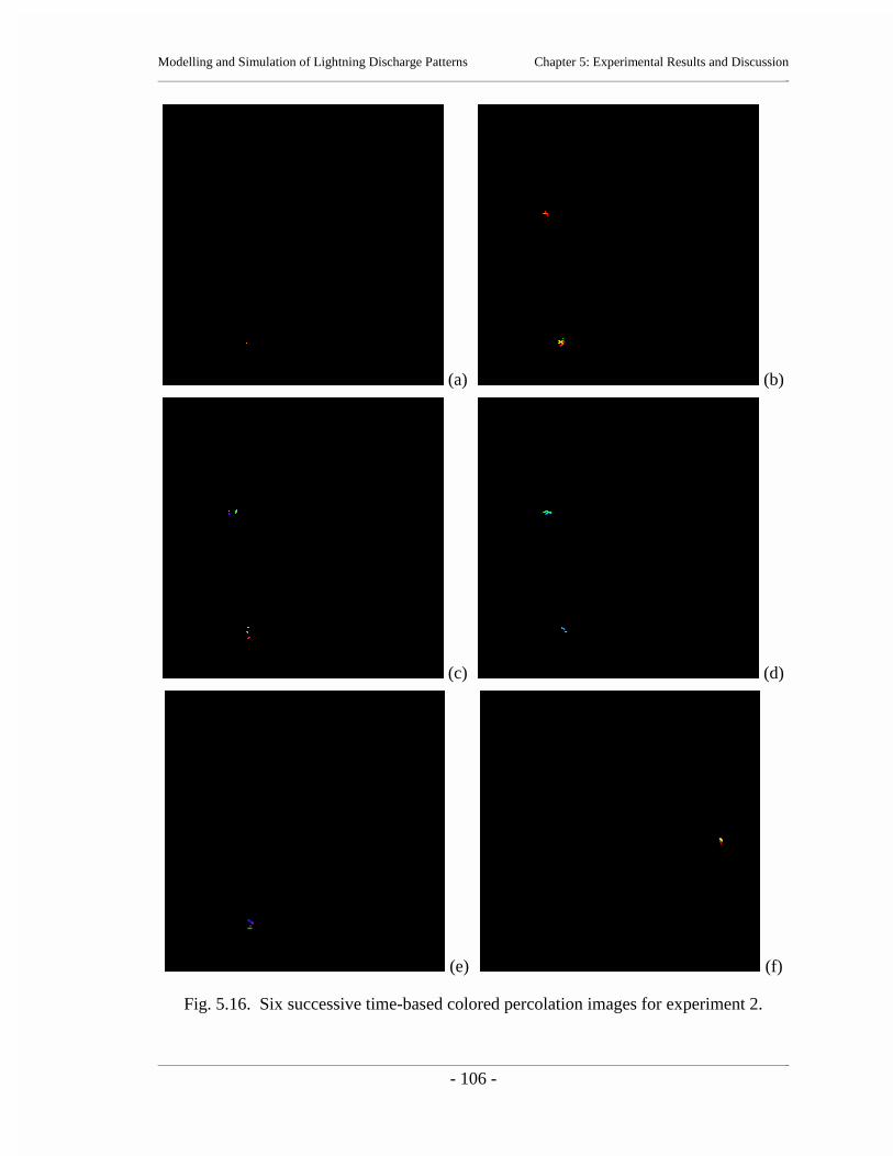
Modelling and Simulation of Lightning Discharge Patterns Chapter 5: Experimental Results and Discussion _
_
- 106 -
(a) (b)
(c) (d)
(e) (f)
Fig. 5.16. Six successive time-based colored percolation images for experiment 2.

Modelling and Simulation of Lightning Discharge Patterns Chapter 5: Experimental Results and Discussion _
_
- 107 -
Fig. 5.17. Rényi dimension spectrum of the black and white images in experiment 2.
The remaining type of analysis to be performed for experiment two is the
quantitative examination using the Rényi dimension spectrum, Fig. 5.17. The first
observation which should be made is the occurrence of the standard dimension curve,
with Dq values ranging primarily between 0.75 and 2. As well, the large change in the
slope of the curve is present about q = 0, confirming the multifractality of the difference
images. Next, it is apparent that the number of frames for which a constant Dq value of
two is present is greater than in the shuttle sequence. This observation substantiates the
earlier conclusion based on visual evidence that the percolation sequence does not

Modelling and Simulation of Lightning Discharge Patterns Chapter 5: Experimental Results and Discussion _
_
- 108 -
contain a sufficient amount of lightning activity. Increasing the number of seeds will
assist in the reduction of these sets of frames for which no changes occur. On the other
hand, the amount of ripple present in the dimension value, with respect to frame number,
for negative values of q, is very little, as seen in the shuttle sequence spectrum. When
positive q values are considered, the ripple produced by the change in the dimension
slope, with respect to frame number, is slightly greater than in the shuttle images. This
increased ripple establishes that the images generated through percolation in this
experiment are more sensitive to the pj probability values than the actual shuttle images.
5.5.4 Experiment 3
The third main experiment in this thesis is very similar to the second, as only an
increase in the number of seeds used in percolation is present. The major percolation
parameters employed in this trial are given in Table 5.4. Three sets, black and white,
height-based coloring and time-based coloring, of six successive images from the
resulting sequences are shown in Fig. 5.18, Fig. 5.19 and Fig. 5.20, respectively. As
well, the computed Rényi dimension spectrum over the entire sequence is plotted in Fig.
5.21.
Table 5.4. Percolation parameter values selected for experiment 3.
Experiment Lattice Lattice Spreading Number of Compression SkippingNumber Side Length Height Probability Seeds Factor Factor
3 256 1300 0.725 1500 5 3
Once again, the analysis process for experiment three shall begin with the
examination of the still images resulting from the percolation simulation. First, it is noted

Modelling and Simulation of Lightning Discharge Patterns Chapter 5: Experimental Results and Discussion _
_
- 109 -
that the size of the lightning flashes is consistent with those seen in the shuttle video,
which is expected since the spreading probability has not changed between experiments
two and three. Next, it is noted that the solidity of each flash is more representative of
actual lightning discharges due to the reduced spreading probability and the use of the
compression factor. The major improvement of this experiment over those previous is
the presence of an increased number of discharges. This expansion activity is generated
from the use of a greater number of seeds in the simulation.
At this point, the results of experiment three are reviewed in their video format.
An initial observation made through the viewing of the animation sequences is that the
number of lightning flashes present in this experiment does indeed more closely match
the number in the shuttle videos, as discerned earlier from the still images. In addition,
the size of the discharges is seen to be more representative of actual lightning flashes.
Once again, the occasional larger bursts of lightning which occur in the shuttle video may
also be seen in the simulation sequence. Since the same spreading probability is used in
both experiments three and two, the percolative growth and decay of flashes is clearly
visible in these results and provides a proper representation of the movement of actual
lightning discharges, as seen in the black and white shuttle video. The only significant
apparent discrepancy between the percolation video and the shuttle video is, again, the
seemingly different frame rates of the two animations. Correction of this observed speed
difference may be possible with an increase in the skipping factor. However, the size of
the lattice required to perform such a simulation is approximately 256 × 256 × 1850,
which would likely require between 450 and 500 MB of memory to maintain high
execution speeds.

Modelling and Simulation of Lightning Discharge Patterns Chapter 5: Experimental Results and Discussion _
_
- 110 -
(a) (b)
(c) (d)
(e) (f)
Fig. 5.18. Six successive black and white percolation images for experiment 3.

Modelling and Simulation of Lightning Discharge Patterns Chapter 5: Experimental Results and Discussion _
_
- 111 -
(a) (b)
(c) (d)
(e) (f)
Fig. 5.19. Six successive height-based colored percolation images for experiment 3.

Modelling and Simulation of Lightning Discharge Patterns Chapter 5: Experimental Results and Discussion _
_
- 112 -
(a) (b)
(c) (d)
(e) (f)
Fig. 5.20. Six successive time-based colored percolation images for experiment 3.

Modelling and Simulation of Lightning Discharge Patterns Chapter 5: Experimental Results and Discussion _
_
- 113 -
Fig. 5.21. Rényi dimension spectrum of the black and white images in experiment 3.
Finally, a quantitative analysis of the results obtained in experiment three is
undertaken using the plot of the Rényi dimension spectrum, as seen in Fig. 5.21. The
characteristic Rényi curve is apparent with dimension values occurring between 0.8 and
2, and rapid descent about q = 0, confirming the multifractality of the lightning difference
images. Another point of interest in the Rényi dimension spectrum of experiment three is
an observable decrease in the number of frames for which the dimension is constant at a
value of two. This reduction confirms the belief that more lightning activity is present,
since these frames with constant Dq equal to 2 are indicative of the lack of change
between frames caused by sparse lightning occurrences. However, the number of such

Modelling and Simulation of Lightning Discharge Patterns Chapter 5: Experimental Results and Discussion _
_
- 114 -
frames is still slightly higher than visible in the shuttle spectrum, meaning that lightning
activity should be increased slightly further. Similar to the previous experiments, the
degree of rippling with respect to frame number for negative values of q is quite low, as
in the shuttle plot. In addition, the Rényi dimension spectrum in this experiment more
closely matches the desired spectrum when the dimension variation, with respect to frame
number, is considered for positive values of q. Hence, modelling using this set of
parameters, with the increase in seeds over experiment two, provides a closer
approximation of the sensitivity to higher pj values and discharge non-stationarity
displayed in the shuttle video.
5.5.5 Experiment 4
The last of the major experiments performed using the percolation lightning
discharge model is now presented and discussed. The percolation parameters chosen for
this simulation are listed in Table 5.5. Six frames from each of the resulting black and
white, height-based color and time-based color images are given in Fig. 5.22, Fig. 5.23
and Fig. 5.24, respectively. The plot of the Rényi dimension spectrum of the entire
sequence of frames is displayed in Fig. 5.25.
Table 5.5. Percolation parameter values selected for experiment 4.
Experiment Lattice Lattice Spreading Number of Compression SkippingNumber Side Length Height Probability Seeds Factor Factor
4 256 1300 0.700 1500 5 3
The first form of analysis performed on this experiment is the assessment of the
selected six images from the sequence. It is immediately apparent that the decrease in the

Modelling and Simulation of Lightning Discharge Patterns Chapter 5: Experimental Results and Discussion _
_
- 115 -
spreading probability has lead to an increase in the size of the percolation clusters.
Consequently the size of the lightning flashes is somewhat large when compared with
those in the shuttle images. As well, the combination of the low spreading probability
and the high number of seeds has caused the number of discharges to be increased
substantially. However, in actuality, this observed rate is not significantly higher than
that seen in the shuttle sequence. When one individual flash is examined, it can be
noticed that a fairly large portion of black speckles is present, likely due to the lower
spreading probability, which allows percolation to form more complex patterns. To
compensate for this fact, a greater compression factor may be required.
The next segment of analysis for experiment four is based upon the video created
from the sequence of percolation images. As expected, the percolation video clearly
demonstrates the presence of quite large lightning flashes caused by the low value for the
spreading probability. As well, the number of discharges is seen to be larger than in
previous experiments, due to the lower spreading probability and the higher number of
seeds, although not unreasonably larger than that in the shuttle video. The growth and
decay of the individual lightning flashes in this video is extremely fractal in nature, and
as a result, too much movement in space is present. This effect, too, is a result of the
spreading probability of 0.7. The appearance of nonsolid lightning flashes as a result of
the complex percolation formations is even more noticeable in the video than in the still
images. Finally, the video in this experiment also suffers from the seemingly different
frame rate than the shuttle video, however, this effect is somewhat masked by the wealth
of lightning activity occurring.

Modelling and Simulation of Lightning Discharge Patterns Chapter 5: Experimental Results and Discussion _
_
- 116 -
(a) (b)
(c) (d)
(e) (f)
Fig. 5.22. Six successive black and white percolation images for experiment 4.

Modelling and Simulation of Lightning Discharge Patterns Chapter 5: Experimental Results and Discussion _
_
- 117 -
(a) (b)
(c) (d)
(e) (f)
Fig. 5.23. Six successive height-based colored percolation images for experiment 4.

Modelling and Simulation of Lightning Discharge Patterns Chapter 5: Experimental Results and Discussion _
_
- 118 -
(a) (b)
(c) (d)
(e) (f)
Fig. 5.24. Six successive time-based colored percolation images for experiment 4.

Modelling and Simulation of Lightning Discharge Patterns Chapter 5: Experimental Results and Discussion _
_
- 119 -
The examination of the Rényi dimension spectrum of the percolation sequence of
experiment four, Fig. 5.25, reveals a number of interesting features. Although the
dimension curves shown in this plot conform to the typical Rényi dimension curves,
including the dominating slope gradient about q = 0, the dimensions themselves range
between values of approximately 1.1 and 2.1 in this experiment. This variance is
indicative of the large percolation clusters visible in the images caused by the lower
spreading probability. Since these structures cause occupation of a more significant
portion of the difference images, the fractal structure is beginning to possess an
appearance closer to that of a solid box, which has a dimension of 2. In addition, the lack
of frames with a constant dimension value of two is visible in the spectrum plot. This
absence confirms the presence of a large amount of lightning activity, since no two
successive frames in the sequence are the same. A final noteworthy point for the Rényi
graph deals with occurrence of fairly severe variation in Dq values, with respect to frame
number, for both negative and positive values of q. These ripples are not nearly as
extreme in the shuttle images and their presence in the percolation spectrum reflects the
intense non-stationarity seen in the video.

Modelling and Simulation of Lightning Discharge Patterns Chapter 5: Experimental Results and Discussion _
_
- 120 -
Fig. 5.25. Rényi dimension spectrum of the black and white images in experiment 4.
5.5.6 Percolation Image Coloring Techniques
In the case of coloring using column heights, as seen in Fig. 5.11, Fig. 5.15, Fig.
5.19 and Fig. 5.23, it can be noted that flashes first appear in the images with colors
which are more “hot” (reds, yellows and greens), and as they fade away, the color
progresses through the cooler shades (blues, purples and pinks). Another visible effect
which can be seen in the images is the predominance of cooler colors. This occurs
because a global maximum connected column height is maintained and used in the
mapping from height to color, as opposed to normalising the values in each individual

Modelling and Simulation of Lightning Discharge Patterns Chapter 5: Experimental Results and Discussion _
_
- 121 -
column with respect to the local maximum height. Consequently, the majority of pixels
are mapped to cooler shades, as their slight variation in heights over time is fairly
insignificant when compared to the large maximum which was likely generated by one or
two widely spreading flashes. Although this method of coloring does not reflect the
growth of individual portions of a flash with time, it does provide a description of the
overall persistence of the lightning discharge through time.
The use of color based on percolation filling time, as shown in Fig. 5.12, Fig.
5.16, Fig. 5.20 and Fig. 5.24, produces significantly different results than the height-
based scheme. An initial observation made from these figures is that a more diverse use
of color is obtained with the time-based method than with the height-based method. This
feature is due to the percolation times being normalised to the local maximum spreading
time for each seed. Although some progression through the spectrum from reds to
purples can be seen, the use of color appears mostly random in these images. This
observation suggests that the time in which a square was filled during the percolation
does not correlate particularly well with the growth of lightning flashes in the sequence
over time. This fact is not entirely surprising, since the source of time progression in the
sequence is solely height-based. In percolation, time is somewhat related to spatial
spreading from a seed, but not entirely representative of this growth since the percolation
process may backtrack or form long offshoots due to the degree of randomness in the
algorithm. The filling time in percolation is determined more by the presence of a fixed
time step clock. As a result, the use of coloring based on percolation filling time is not
overly effective as a indicator of flash growth with time in the image sequences.

Modelling and Simulation of Lightning Discharge Patterns Chapter 5: Experimental Results and Discussion _
_
- 122 -
However, one interesting aspect of the percolation model can be observed through
comparison of the lightning locations and sizes in the two coloring methods, namely the
direct effects of the compression factor. The height-based colored images are generated
using the compressed lattice while for ease of computation, the time-based images are
constructed before the lattice is compressed. By examining corresponding images, it is
seen that the compressed-based images produce lightning flashes which are much more
full and less speckled than those seen in the uncompressed images. Hence, the use of the
compression factor does indeed produce lightning images which more closely resemble
those gathered from shuttle videos.
5.5.7 Summary of Results
The results and analysis of the experiments presented in the previous subsections
allow a number of comments to be made pertaining to the parameter variation trends and
the overall usability of the percolation system.
To begin, the value of the spreading probability is seen to play an integral role in
the output images. The primary effect of altering this parameter is a change in size of the
lightning flashes. An ideal value appears to be 0.725. Even small deviations from this
value cause rather large or quite small discharges to be produced.
The other major parameter which is varied throughout the course of the four
experiments is the number of percolation seeds used. Rather large changes in this value
are required to create noticeable differences in the output. A value of 1500 is found to
generate a reasonable number of lightning discharges.

Modelling and Simulation of Lightning Discharge Patterns Chapter 5: Experimental Results and Discussion _
_
- 123 -
The remaining major parameters of lattice size, compression factor and skipping
factor are not varied through the experiments, yet the effects of these variable are clearly
visible. The skipping factor alters the perceived frame rate of the resulting videos. A
value of three is used for this factor due to memory limitations, however, the output
videos still appear slow in comparison with the shuttle video. The compression factor is
responsible for the elimination of some of the observed black speckles within a given
lightning flash, due to the complexity of percolation. The value for this factor is selected
to be five, and appears to perform adequately for the more optimal values of the other
percolation parameters.
The four experiments outlined in the previous subsections are all within the realm
of possible lightning storms. The sequence of experiment one is representative of a storm
for which little lightning activity is present. Experiments two and three produce results
which could be used to describe a medium sized storm with moderate lightning. Finally,
experiment four presents the model of an extremely intense thunderstorm.
5.6 Summary
This chapter is responsible for the verification of the lightning modelling system,
as well as experimentation with its usage to ascertain the types of simulations which the
percolation model is capable of producing.
The system is verified based upon its major components, while their interaction is
proven during the experimental phase. This validation is achieved by analysing the
Rényi dimension spectrum program, the shuttle image processing program and the
percolation program.

Modelling and Simulation of Lightning Discharge Patterns Chapter 5: Experimental Results and Discussion _
_
- 124 -
This chapter then develops the experiments which are to be run using the
modelling software. The experiments are designed carefully, based upon basic trial runs
to establish reasonable parameter values, so as to determine the various formations which
can be generated, while still remaining in the relevant domain of lightning discharges.
The experimentation portion of this chapter is divided into five distinct
components, namely the use of the shuttle image analysis program and four percolation
experiments. The purpose of the shuttle experiment is to illustrate further the output of
this component of the system. The four experiments contain different sets of percolation
parameter values. These trials establish trends caused by the variation of these
parameters and isolate a particular set which generates quite accurate lightning discharge
simulations.

Modelling and Simulation of Lightning Discharge Patterns Chapter 6: Conclusions and Recommendations _
_
- 125 -
CHAPTER 6 CONCLUSIONS AND RECOMMENDATIONS
6.1 Conclusions
The purpose of this thesis is to develop and implement a model which is capable
of simulating lightning discharge patterns observed from above during space shuttle
missions. The motivation for the creation of such a system is the insight which it will
provide into thunderstorm processes themselves. This knowledge may then be used to
assist in the pursuit of the ultimate goal of thunderstorm trajectory prediction.
The basis for the new lightning model described in this thesis is selected to be
percolation theory. With only slight refinements, the standard percolation process may
be used in three dimensions to generate sequences of images which model black and
white versions of space shuttle lightning videos. A number of experiments are undergone
to establish the capabilities of the percolation model, and a quantitative fractal
comparison of the resulting images with a representative shuttle sequence is performed.
These experiments illustrate that a wide range of lightning simulations can be
produced by the percolation model simply by varying a few key parameters.
Specifically, the effects of varying the percolation spreading probability and the number
of seeds utilised are studied, and general trends are found. The percolation model is
sensitive to even slight changes in the spreading probability, with the most accurate
results being produced with a value of 0.725. Through the variation of this parameter,
different sized lightning discharges can be generated. Higher values of the spreading

Modelling and Simulation of Lightning Discharge Patterns Chapter 6: Conclusions and Recommendations _
_
- 126 -
probability, such as 0.73, result in simulations which can be used to demonstrate storms
for which little lightning activity is present. Lower values of the spreading probability,
for example 0.7, produce sequences for which extensive electrical activity is occurring.
The other focal parameter in the percolation simulations is the number of seeds used.
This parameter must be varied by significantly greater amounts to produce noticeable
changes in output bitmaps. Experiments are run using values of 1000 and 1500 seeds,
and this parameter is determined to influence the number of lightning discharges present
in the sequences. The experiments in which 1500 seeds are chosen resulted in the
creation of lightning videos with moderate sized storms.
The quantitative metric of the Rényi dimension spectrum is used to concretely
verify the visual conclusions drawn by observing both still images and video sequences.
This measure is applied to images representing differences between successive lightning
frames. It is found that the experiment using a spreading probability of 0.725 and 1500
seeds conforms to the spectrum of the selected shuttle sequence. This spectrum is one in
which dimension values vary approximately between 1 and 2, with almost no variation
over time for negative moment orders and slight ripples over time for positive moment
orders. Hence, the Rényi dimension spectrum illustrates the multifractality of lightning
discharges in both space and time. As well, this spectrum contains a small portion of
completely black frames, representing no change in the actual lightning sequence for two
successive frames.
The experimental results presented in this thesis clearly demonstrate that the
percolation model can generate lightning image sequences which are both qualitatively
and quantitatively representative of those fractal patterns visible for typical

Modelling and Simulation of Lightning Discharge Patterns Chapter 6: Conclusions and Recommendations _
_
- 127 -
thunderstorms. As well, the percolation lightning discharge model has the ability to
create sequences portraying both unrealistically large and small thunderstorms,
demonstrating the behavioral characteristics and conditions behind these natural
phenomena.
6.2 Recommendations
A number of recommendations are possible as to the future research extensions in
the use of percolation to model lightning discharge patterns. A selection of these
suggestions are as follows:
• The implementation of the Rényi dimension spectrum calculation contains some
inefficiencies which are used simply to increase the ease of coding. However, the
resulting program does not run as quickly as desired. Hence, this code could be
optimised to decrease the computation time required by this program.
• Since the focus of this thesis is the development and implementation of the
percolation model itself to test the feasibility of its use as a lightning discharge
simulation technique, a graphical user interface is not developed. With the promise
of the model now established, the creation of a GUI would significantly increase the
system’s usability.
• Although the major functionality of the percolation model has been displayed through
the four major experiments in this thesis, only a small fraction of the available
combinations of the percolation parameters have been examined. Hence, further

Modelling and Simulation of Lightning Discharge Patterns Chapter 6: Conclusions and Recommendations _
_
- 128 -
testing of the capabilities of the percolation model would likely prove quite
enlightening.
• The purpose of the use of color in the percolation image sequence is to illustrate the
growth of individual lightning discharges with time. The height-based coloring does
provide an indication of the position within the overall lifespan of a given flash,
however, it does not illustrate the growth of the discharge on a smaller, say single
time step, basis. Consequently, refinements to the coloring algorithms could be made
to better reflect this procession.
• This thesis demonstrates that the percolation model is successful in accurately
representing the lightning discharge patterns observed from the space shuttle.
However, only one such shuttle video is used for comparison purposes. Although it is
believed that this technique does model the underlying structure common to
thunderstorms in general, the system should be tested against other shuttle sequences
to determine the percolation parameters required and the relative accuracy of the
system.
6.3 Contributions
The contributions made by the research and development of this thesis may be
summarised as follows:
• The brief summarisation and commentary on the current techniques used to model
lightening discharge patterns.

Modelling and Simulation of Lightning Discharge Patterns Chapter 6: Conclusions and Recommendations _
_
- 129 -
• The development and implementation of a percolation-based model capable of
simulating lightning sequences recorded from the space shuttle.
• The experimentation using the percolation modelling software to determine the
operation range of the model and the effects of the various parameters.
• The expanse of the diversity of applications for which percolation may be employed.
• The development of my personal image processing and modelling skills as well as my
understanding of fractals and disordered systems.

Modelling and Simulation of Lightning Discharge Patterns References _
_
- 130 -
REFERENCES
[Aren96] L. Arendt, “Stochastic modelling and multifractals characterisation ofdielectric discharges using Laplacian fractals,” M.Sc. Thesis, Dept.Electrical & Computer Engineering, University of Manitoba, Sept. 1996,311 pp.
[BuHa91] A. Bunde and S. Havlin, Fractals and Disordered Systems. New York,NY: Springer-Verlag, 1991, 350 pp.
[CaKi00] J. Cannons and W. Kinsner, “Modelling of lightning discharge patterns asobserved from space,” Mathematical Modelling and Scientific Computing,vol. 10, 2000, 8 pages submitted.
[Dool98a] D. Dooling, “Space science news,”http://science.msfc.nasa.gov/newhome/headlines/essd19may98_2.htm, asof 21 February 2000.
[Dool98b] D. Dooling, “Space science news,”http://science.msfc.nasa.gov/newhome/headlines/essd24aug98_2.htm, asof 21 February 2000.
[Envi99] Environment Canada, “Satellite images,”http://www.cmc.ec.gc.ca/cmc/htmls/satellite.html, as of 7 June 1999.
[Fede88] J. Feder, Fractals. New York, NY: Plenum Press, 1988, 283 pp.
[Good99a] M. Goodman, “Lightning detection and ranging (LDAR) datasetsummary,” http://wwwghrc.msfc.nasa.gov/uso/readme/ldar.html, as of 4March 2000.
[Good99b] S. Goodman, “LDAR browse calendar,”http://thunder.msfc.nasa.gov/lightning-cgi-bin/ldar/ldar_browse.pl, as of30 May 1999.
[Good00a] S. Goodman, “Lightning detection from space, A lightning primer,”http://thunder.msfc.nasa.gov/primer/, as of 4 March 2000.
[Good00b] S. Goodman, “Space research and observations, Space shuttle lightningexperiments,” http://thunder.msfc.nasa.gov/shuttle.html, as of 4 March2000.

Modelling and Simulation of Lightning Discharge Patterns References _
_
- 131 -
[Harr99] S. Harrison, “National lightning detection network (NLDN) of improvedperformance from combined technology (IMPACT) radio frequencyantenna system,”http://ghrc.msfc.nasa.gov:5721/sensor_documents/NLDN_antenna.html,as of 4 March 2000.
[HaNK89] W. W. Hager, J. S. Nisbet, and J. R. Kasha, “The evolution and dischargeof electric fields within a thunderstorm,” J. of Computational Physics, vol.82, pp. 193-217, 1989.
[Kins94] W. Kinsner, “Fractal and Chaos Engineering,” Course Notes, Dept.Electrical & Computer Engineering, University of Manitoba, 1994.
[LeBT83] Z. Levin, W. J. Borucki, and O. B. Toon, “Lightning generation inplanetary atmospheres,” Icarus, vol. 56, pp. 80-115, 1983.
[LeTz86] Z. Levin and I. Tzur, “Models of the development of the electricalstructure of clouds,” in The Earth’s Electrical Environment, Studies inGeophysics. Washington, D.C.: National Academic Press, pp. 131-145,1986.
[Mcgu91] M. McGuire, An Eye for Fractals. Redwood City, CA: Addison-Wesley,1991.
[Micr99] Microsoft Corporation, “Microsoft Encarta Encyclopaedia 99”, 1999.
[Mill00] T. Miller, “Optical transient detector,”http://wwwghcc.msfc.nasa.gov/OTD/images/OKstorm_OTDflash_NLDNflash.gif, as of 21 February 2000.
[Moll00] A. Moller, “Lightning,”http://ww2010.atmos.uiuc.edu/(Gh)/guides/mtr/svr/dngr/light.rxml, as of21 February 2000.
[Nati00] National Weather Service, “The WSR-88D doppler radar,”http://www.jannws.state.ms.us/wsr88d1.html, as of 4 March 2000.
[NoBL91] K. Norville, M. Baker, and J. Latham, “A numerical study of thunderstormelectrification: Model development and case study,” J. of GeophysicalResearch, vol. 96(D4), pp. 7463-7481, 1991.
[PeJS92] H. Peitgen, H. Jürgens, and D. Saupe, Chaos and Fractals. New York,NY: Springer-Verlag, 1992.
[PVSH92] D. E. Pitts, O. H. Vaughan Jr., C. A. Sapp, D. Helms, M. Chambers, P.Jaklitch, and M. Duncan, “Analysis of lightning flash video from the spaceshuttle using blob and morphological techniques,” InternationalGeoscience and Remote Sensing Symposium, vol. 2, pp. 1556-1558, 1992.

Modelling and Simulation of Lightning Discharge Patterns References _
_
- 132 -
[Rinn85] K. Rinnert, “Lightning on other planets,” J. of Geophysical Research, vol.90(D4), pp. 6225-6237, 1985.
[SeWe93] D. Sentman and E. Wescott, “Observations of upper atmospheric opticalflashes recorded from an aircraft,” Geophysical Research Letters, vol. 20,no. 24, pp. 2857-2860, 1993.
[Stac94] G. Stacey, “Stochastic fractals modelling of dielectric discharges,” M.Sc.Thesis, Dept. Electrical & Computer Engineering, University of Manitoba,Nov. 1994, 308 pp.
[Syst99] Systems Acquisition Office, National Oceans and AtmosphericAdministration, “Geostationary operational environmental satellite(GOES) acquisition,” http://www.sao.noaa.gov/goes/goes.html, as of 4March 2000.
[VaMP98] J. Valdivia, G. Milikh, and K. Papadopoulos, “Model of red sprites due tointracloud fractal lightning discharges,” Radio Science, vol. 33, no. 6, pp.1655-1668, 1998.
[Vaug97] O. H. Vaughan, Jr., “Space shuttle observations of lightning - Mesoscalelightning experiment,” http://www.ghcc.msfc.nasa.gov/skeets.html, as of21 February 2000.
[Vics92] T. Vicsek, Fractal Growth Phenomena. River Edge, NJ: World Scientific,1992 (2nd ed.), 488 pp.
[Whip82] A. Whipple, Storm. Alexandria, Virginia: Time-Life Books, 1982.
[Wsic99] Weather Services International, http://www.wsicorp.com, as of 2September 1999.
[YaLT95] Y. Yair, Z. Levin, and S. Tzivion, “Lightning generation in a Jovianthundercloud: Results from an axisymmetric numerical cloud model,”Icarus, vol. 115, pp. 421-434, 1995.

Modelling and Simulation of Lightning Discharge Patterns Appendix A: Software Listing _
_
- A1 -
APPENDIX A: SOFTWARE LISTING
A.1 InitUnit.h
/* This unit contains type definitions and constants used by the majority of the simulation programs. */
/* include files */
#ifdef PC32 #include <windows.h> /* For 32-bit machines only */#endif
/* type */
#ifdef PC16 //typedef unsigned short int WORD; /* TypeDef WORD to 16 bits, only VC */ typedef unsigned int WORD; /* TypeDef WORD to 16 bits, only TC */ typedef unsigned long int DWORD; /* TypeDef DWORD to 32 bits */ typedef unsigned char BYTE; /* TypeDef BYTE to 8 bits */ #endif
#ifdef LINUX typedef unsigned char BYTE; /* TypeDef BYTE to 8 bits */ typedef unsigned short int WORD; /* TypeDef WORD to 16 bits */ typedef unsigned int DWORD; /* TypeDef DWORD to 32 bits */ #endif
#ifdef UNIX typedef unsigned char BYTE; /* TypeDef BYTE to 8 bits */ typedef unsigned short int WORD; /* TypeDef WORD to 16 bits */ typedef unsigned int DWORD; /* TypeDef DWORD to 32 bits */ #endif
/* const */
#define XMax 256 #define YMax 256 #define ZMax 1300 /* x, y and z y max of lattice */ /* NOTE: Make sure that XMax * YMax is divisible by 8!! */
#define Scale 2 /* Factor by which to scale the output bmps */
#define Dead 3 #define FilledND 2 #define FilledD 1 #define Empty 0 /* Map pixel states to integers: */ /* dead, filled and not done, filled and done, empty */
#define TotFrames 300 /* Total number of frames generated */

Modelling and Simulation of Lightning Discharge Patterns Appendix A: Software Listing _
_
- A2 -
A.2 FileUnit.h
/* This unit contains all type and procedure / function declarations used in the managing of the files. */
/* interface */
#include <stdio.h>
#ifdef PC32 #include <windows.h> /* For 32-bit machines only */#endif
/* type */
#ifdef PC16 //typedef unsigned short int WORD; /* TypeDef WORD to 16 bits, only VC */ typedef unsigned int WORD; /* TypeDef WORD to 16 bits, only TC */ typedef unsigned long int DWORD; /* TypeDef DWORD to 32 bits */ typedef unsigned char BYTE; /* TypeDef BYTE to 8 bits */ #endif
#ifdef LINUX typedef unsigned char BYTE; /* TypeDef BYTE to 8 bits */ typedef unsigned short int WORD; /* TypeDef WORD to 16 bits */ typedef unsigned int DWORD; /* TypeDef DWORD to 32 bits */ #endif
#ifdef UNIX typedef unsigned char BYTE; /* TypeDef BYTE to 8 bits */ typedef unsigned short int WORD; /* TypeDef WORD to 16 bits */ typedef unsigned int DWORD; /* TypeDef DWORD to 32 bits */ #endif
void InitFile (char *DirName, int Frame, FILE * & File, char *RW);/* This procedure initializes the file. */

Modelling and Simulation of Lightning Discharge Patterns Appendix A: Software Listing _
_
- A3 -
A.3 FileUnit.cpp
/* This unit contains all type and procedure / function declarations used in the managing of the files. */
/* implementation */
#include "FileUnit.h"#include <stdio.h>#include <stdlib.h>#include <string.h>
/* ----------------------------------------------------------------------- */
void InitFile (char *DirName, int Frame, FILE * & File, char *RW)/* This procedure initializes the file. */
{ char Temp [256] = ""; /* Temporary string for fopen */ int Digit; /* Temporary current digit of frame number */ char Letter [2]; /* Temporary string value of current digit */ int Index; /* Loop counter to pull off digits */
strcat (Temp, DirName); /* Add on directory */
for (Index = 1000; Index >= 1; Index = Index / 10) { /* For each of the 4 digits in the frame number starting at left */ Digit = (Frame / Index) % 10; /* Pull off correct digit */ Letter [0] = '0' + Digit; /* Convert to char */ Letter [1] = 0; /* Add null termination */ strcat (Temp, Letter); /* Add to string */ }
if (! strcmp (RW, "wb") || ! strcmp (RW, "rb")) /* If is a binary file */ if (strstr (Temp, "Stat") != NULL) /* check if is a status file */ strcat (Temp, ".sta"); else if (strstr (Temp, "Time") != NULL) /* check if a time file */ strcat (Temp, ".tim"); else if (strstr (Temp, "Hgt") != NULL) /* if height file */ strcat (Temp, ".hgt"); else strcat (Temp, ".bmp"); /* else assume bmp */ else strcat (Temp, ".txt"); /* else add txt extension */ File = fopen (Temp, RW); /* Open the file */ if (File == NULL) { printf ("Can't open file"); fflush (stdout); exit (0); }} /* InitFile */

Modelling and Simulation of Lightning Discharge Patterns Appendix A: Software Listing _
_
- A4 -
A.4 bmpunit.h
/* This unit contains all type and procedure / function declarations used in the managing of bitmap files. */
/* interface */
#include <stdio.h>
#ifdef PC32 #include "..\InitUnit\InitUnit.h"#endif
#ifdef UNIX #include "../InitUnit/InitUnit.h"#endif
#ifdef LINUX #include "../InitUnit/InitUnit.h"#endif
/* type */
#ifdef PC32 #pragma pack (push, 1) /* For 32-bit machines only */ #endif
#ifdef UNIX #pragma pack (1) /* For UNIX */ #endif
#ifdef LINUX #pragma pack (1) /* For LINUX */ #endif
typedef struct _BmpHeaderType /* Record type for a 3.x bmp header */ { WORD ImageFileType; /* Image file type, always 424Dh ("BM") */ DWORD FileSize; /* Physical file size in bytes */ WORD Reserved1; /* Always 0 */ WORD Reserved2; /* Always 0 */ DWORD ImageDataOffset; /* Start of image data offset in bytes */ } BmpHeaderType;
typedef struct _BmpInfoHeaderType { /* Record type for a 3.x bmp info header */ DWORD HeaderSize; /* Size of this header */ DWORD ImageWidth; /* Image width in pixels */ DWORD ImageHeight; /* Image height in pixels */ WORD NumberofImagePlanes; /* Number of planes (always 1) */ WORD BitsPerPixel; /* Bits per pixel (1, 4, 8 or 24) */ DWORD CompressionMethod; /* Compression method used (0, 1, or 2) */ /* 0 = uncompressed, 1 = 8-bit RLE, 2 = 4-bit RLE */ DWORD SizeOfBitmap; /* Size of the bitmap in bytes */ DWORD HorizRes; /* Horizontal resolution in pixels per meter */ DWORD VertRes; /* Vertical resoltion in pixels per meter */ DWORD NumColorsUsed; /* Number of colors in the image */ DWORD NumSigColors; /* Number of important colors in palette */ } BmpInfoHeaderType;
typedef struct _RGBType /* Record type for one RGB pixel */

Modelling and Simulation of Lightning Discharge Patterns Appendix A: Software Listing _
_
- A5 -
{ BYTE R; /* One byte for */ BYTE G; /* each of R, G and B */ BYTE B; /* For "grayscale", R = G = B */ } RGBType;
#ifdef PC32 #pragma pack (pop) /* For 32-bit machines only */ #endif
typedef struct _BmpDataType /* Record type for bmp data */ { RGBType **Array; /* 2D array of bmp pixels (of RGBType) */ DWORD Width; /* Width of array */ DWORD Height; /* Height of array */ } BmpDataType;
void ReadBmpHeaders (FILE *InFile, BmpHeaderType & BmpHeader, BmpInfoHeaderType & BmpInfoHeader);/* This procedure reads in the bmp header and info header from InFile. */
void FixBmpHeaders (BmpHeaderType & BmpHeader, BmpInfoHeaderType & BmpInfoHeader);/* This procedure fixes the BigEndian / LittleEndian conflict for Unix boxes. */
void CreateBmpHeaders (BmpHeaderType & BmpHeader, BmpInfoHeaderType & BmpInfoHeader, DWORD Height, DWORD Width);/* This procedure creates the bmp header and info header. */
void WriteBmpHeaders (BmpHeaderType BmpHeader, BmpInfoHeaderType BmpInfoHeader, FILE *OutFile);/* This procedure writes the bmp header and info header to the OutFile. */
void WriteBmpData (FILE *OutFile, BmpDataType BmpData);/* This procedure writes the bmp data to the file. */
void PrintBmpData (BmpDataType BmpData);/* This procedure prints the bmp data to the screen. */
void WriteBmpPixel (FILE *OutFile, RGBType Pixel);/* This procedure writes the bmp pixel to the file. */
void ReadBmpPixel (FILE *InFile, RGBType & Pixel);/* This procedure reads a bmp pixel from the file. */
void PrintBmpHeaders (BmpHeaderType BmpHeader, BmpInfoHeaderType BmpInfoHeader);/* This procedure prints out the contents of the two bmp headers. */
void SetWidthAndHeight (BmpDataType & BmpData, BmpInfoHeaderType BmpInfoHeader);/* This procedure sets the height and width fields in BmpData as specified in BmpInfoHeader. */
void GetBmpDataSpace (BmpDataType & BmpData);/* This procedure allocates an amount of memory for the bmp data as calulated from the image height and width. */
void FreeBmpDataSpace (BmpDataType & BmpData);/* This procedure frees the memory allocated for the bmp array. */

Modelling and Simulation of Lightning Discharge Patterns Appendix A: Software Listing _
_
- A6 -
void ReadBmpData (FILE *InFile, BmpDataType BmpData, DWORD ImageDataOffset);/* This procedure reads the bmp data of the specified size, beginning at the specified offset, from the image file into BmpData. */
RGBType PixelGen (BYTE R, BYTE G, BYTE B);/* This function take in the RGB values for a pixel and return the pixel. */
int PixelIntensity (RGBType Pixel);/* This function takes in a pixel and returns it's intensity. */
void FindAvBmpIntensity (BmpDataType BmpData, int & BmpAvIntensity);/* This procedure finds the average intensity of the bmp and stores it in BmpAvIntensity. */

Modelling and Simulation of Lightning Discharge Patterns Appendix A: Software Listing _
_
- A7 -
A.5 bmpunit.cpp
/* This unit contains all type and procedure / function declarations used in the managing of bitmap files. */
/* implementation */
#include "bmpunit.h"#include <stdio.h>#include <stdlib.h>#include <malloc.h>
/* ----------------------------------------------------------------------- */
void ReadBmpHeaders (FILE *InFile, BmpHeaderType & BmpHeader, BmpInfoHeaderType & BmpInfoHeader)/* This procedure reads in the bmp header and info header from InFile. */
{ fread (& BmpHeader, sizeof (BmpHeaderType), 1, InFile); /* Read header */ fread (& BmpInfoHeader, sizeof (BmpInfoHeaderType), 1, InFile); /* Read the info header */} /* ReadBmpHeaders */
/* ----------------------------------------------------------------------- */
void ChangeMeShort (long *var)/* This procedure converts short variables (WORDs) between BigEndian and LittleEndian. */
{ char tmp; /* Temp var for swapping bytes */
tmp = ((char *) var)[0]; ((char *) var)[0] = ((char *) var)[1]; ((char *) var)[1] = tmp;} /* ChangeMeShort */
/* ----------------------------------------------------------------------- */
void ChangeMeLong (long *var)/* This procedure converts long variables (DWORDs) between BigEndian and LittleEndian. */
{ char tmp; /* Temp var for swapping bytes */
tmp = ((char *) var)[0]; ((char *) var)[0] = ((char *) var)[3]; ((char *) var)[3] = tmp;
tmp = ((char *) var)[1]; ((char *) var)[1] = ((char *) var)[2]; ((char *) var)[2] = tmp;} /* ChangeMeLong */
/* ----------------------------------------------------------------------- */
void FixBmpHeaders (BmpHeaderType & BmpHeader, BmpInfoHeaderType & BmpInfoHeader)

Modelling and Simulation of Lightning Discharge Patterns Appendix A: Software Listing _
_
- A8 -
/* This procedure fixes the BigEndian / LittleEndian conflict for Unix boxes. */
{ ChangeMeShort ((long *) & BmpHeader.ImageFileType); /* Fix the header */ ChangeMeLong ((long *) & BmpHeader.FileSize); ChangeMeShort ((long *) & BmpHeader.Reserved1); ChangeMeShort ((long *) & BmpHeader.Reserved2); ChangeMeLong ((long *) & BmpHeader.ImageDataOffset);
ChangeMeLong ((long *) & BmpInfoHeader.HeaderSize); /* Fix info header */ ChangeMeLong ((long *) & BmpInfoHeader.ImageWidth); ChangeMeLong ((long *) & BmpInfoHeader.ImageHeight); ChangeMeShort ((long *) & BmpInfoHeader.NumberofImagePlanes); ChangeMeShort ((long *) & BmpInfoHeader.BitsPerPixel); ChangeMeLong ((long *) & BmpInfoHeader.CompressionMethod); ChangeMeLong ((long *) & BmpInfoHeader.SizeOfBitmap); ChangeMeLong ((long *) & BmpInfoHeader.HorizRes); ChangeMeLong ((long *) & BmpInfoHeader.VertRes); ChangeMeLong ((long *) & BmpInfoHeader.NumColorsUsed); ChangeMeLong ((long *) & BmpInfoHeader.NumSigColors);} /* FixBmpHeaders */
/* ----------------------------------------------------------------------- */
int PixelIntensity (RGBType Pixel)/* This function takes in a pixel and returns it's intensity. */
{ /* NOTE: Assume 24-bit grayscale image (R = G = B) */ return ((unsigned char)Pixel.R);} /* PixelIntensity */
/* ----------------------------------------------------------------------- */
void CreateBmpHeaders (BmpHeaderType & BmpHeader, BmpInfoHeaderType & BmpInfoHeader, DWORD Height, DWORD Width)/* This procedure creates the bmp header and info header. */
{ BmpHeader.ImageFileType = 0x4d42; /* Hex meaning it is a bmp */ BmpHeader.FileSize = Height * Width * 3 + 54; /* NOTE: Assumes 24-bit color */ BmpHeader.Reserved1 = 0; /* Always 0 */ BmpHeader.Reserved2 = 0; /* Always 0 */ BmpHeader.ImageDataOffset = 54; /* 54 bytes to data */
BmpInfoHeader.HeaderSize = 40; /* Info header is 40 bytes long */ BmpInfoHeader.ImageWidth = Width; /* Width in pixels */ BmpInfoHeader.ImageHeight = Height; /* Height in pixels */ BmpInfoHeader.NumberofImagePlanes = 1; /* Always 1 */ BmpInfoHeader.BitsPerPixel = 24; /* NOTE: Assumes 24-bit color */ BmpInfoHeader.CompressionMethod = 0; /* NOTE: Assumes umcompressed */ BmpInfoHeader.SizeOfBitmap = Height * Width * 3; /* NOTE: Assumes 24-bit color */ BmpInfoHeader.HorizRes = 0; /* Just because */ BmpInfoHeader.VertRes = 0; BmpInfoHeader.NumColorsUsed = 0; BmpInfoHeader.NumSigColors = 0;} /* CreateBmpHeaders */
/* ----------------------------------------------------------------------- */

Modelling and Simulation of Lightning Discharge Patterns Appendix A: Software Listing _
_
- A9 -
void WriteBmpHeaders (BmpHeaderType BmpHeader, BmpInfoHeaderType BmpInfoHeader, FILE *OutFile)/* This procedure writes the bmp header and info header to the OutFile. */
{ fwrite (& BmpHeader, sizeof (BmpHeaderType), 1, OutFile); /* Write header */ fwrite (& BmpInfoHeader, sizeof (BmpInfoHeaderType), 1, OutFile); /* Write the info header */
} /* WriteBmpHeaders */
/* ----------------------------------------------------------------------- */
void WriteBmpData (FILE *OutFile, BmpDataType BmpData)/* This procedure writes the bmp data to the file. */
{ DWORD Row; /* Loop counter for current row */ DWORD Col; /* Loop counter for current column */
/* NOTE: Assume 24-bit image with no compression */ /* Write in one pixel at a time from the 2D array */ for (Row = 0; Row < BmpData.Height; Row++) for (Col = 0; Col < BmpData.Width; Col++) fwrite (& BmpData.Array [Col][Row], sizeof (RGBType), 1, OutFile);} /* WriteBmpData */
/* ----------------------------------------------------------------------- */
void PrintBmpData (BmpDataType BmpData)/* This procedure prints the bmp data to the screen. */
{ DWORD Row; /* Loop counter for current row */ DWORD Col; /* Loop counter for current column */
/* NOTE: Assume 24-bit image with no compression */ /* Write in one pixel at a time from the 2D array */ for (Row = 0; Row < BmpData.Height; Row++) { for (Col = 0; Col < BmpData.Width; Col++) if (PixelIntensity (BmpData.Array [Col][Row]) == 255) printf ("1 "); else printf ("0 "); printf ("\n"); } printf ("\n\n");} /* PrintBmpData */
/* ----------------------------------------------------------------------- */
void WriteBmpPixel (FILE *OutFile, RGBType Pixel)/* This procedure writes the bmp pixel to the file. */
{ fwrite (& Pixel, sizeof (RGBType), 1, OutFile);} /* WriteBmpPixel */
/* ----------------------------------------------------------------------- */
void ReadBmpPixel (FILE *InFile, RGBType & Pixel)

Modelling and Simulation of Lightning Discharge Patterns Appendix A: Software Listing _
_
- A10 -
/* This procedure reads a bmp pixel from the file. */
{ fread (& Pixel, sizeof (RGBType), 1, InFile);} /* ReadBmpPixel */
/* ----------------------------------------------------------------------- */
void PrintBmpHeaders (BmpHeaderType BmpHeader, BmpInfoHeaderType BmpInfoHeader)/* This procedure prints out the contents of the two bmp headers. */
{ #ifdef PC32 printf ("Image file type: %hx \n", BmpHeader.ImageFileType); printf ("File size: %lu \n", BmpHeader.FileSize); printf ("Reserved 1: %hu \n", BmpHeader.Reserved1); printf ("Reserved 2: %hu \n", BmpHeader.Reserved2); printf ("Image data offset: %lu \n", BmpHeader.ImageDataOffset); printf ("Header size: %lu \n", BmpInfoHeader.HeaderSize); printf ("Image width: %lu \n", BmpInfoHeader.ImageWidth); printf ("Image height: %lu \n", BmpInfoHeader.ImageH printf ("Number of image planes: %hu \n", BmpInfoHeader.NumberofImagePlanes); printf ("Bits per pixel: %hu \n", BmpInfoHeader.BitsPerPixel); printf ("Compression method: %lu \n", BmpInfoHeader.CompressionMethod); printf ("Size of bitmap: %lu \n", BmpInfoHeader.SizeOfBitmap); printf ("Horizontal resolution: %lu \n", BmpInfoHeader.HorizRes); printf ("Vertical resolution: %lu \n", BmpInfoHeader.VertRes); printf ("Number of colors used: %lu \n", BmpInfoHeader.NumColorsUsed); printf ("Number of significant colors: %lu\n",BmpInfoHeader.NumSigColors); #endif #ifdef UNIX printf ("Image file type: %hx \n", BmpHeader.ImageFileType); printf ("File size: %u \n", BmpHeader.FileSize); printf ("Reserved 1: %u \n", BmpHeader.Reserved1); printf ("Reserved 2: %u \n", BmpHeader.Reserved2); printf ("Image data offset: %hu \n", BmpHeader.ImageDataOffset); printf ("Header size: %hu \n", BmpInfoHeader.HeaderSize); printf ("Image width: %u \n", BmpInfoHeader.ImageWidth); printf ("Image height: %u \n", BmpInfoHeader.ImageHeight); printf ("Number of image planes: %u \n", BmpInfoHeader.NumberofImagePlanes); printf ("Bits per pixel: %u \n", BmpInfoHeader.BitsPerPixel); printf ("Compression method: %hu \n", BmpInfoHeader.CompressionMethod); printf ("Size of bitmap: %hu \n", BmpInfoHeader.SizeOfBitmap); printf ("Horizontal resolution: %hu \n", BmpInfoHeader.HorizRes); printf ("Vertical resolution: %hu \n", BmpInfoHeader.VertRes); printf ("Number of colors used: %hu \n", BmpInfoHeader.NumColorsUsed); printf ("Number of significant colors: %hu\n",BmpInfoHeader.NumSigColors); #endif} /* PrintBmpHeaders */
/* ----------------------------------------------------------------------- */
void SetWidthAndHeight (BmpDataType & BmpData, BmpInfoHeaderType BmpInfoHeader)/* This procedure sets the height and width fields in BmpData as specified in BmpInfoHeader. */
{ BmpData.Width = BmpInfoHeader.ImageWidth; BmpData.Height = BmpInfoHeader.ImageHeight;

Modelling and Simulation of Lightning Discharge Patterns Appendix A: Software Listing _
_
- A11 -
} /* SetWidthAndHeight */
/* ----------------------------------------------------------------------- */
void GetBmpDataSpace (BmpDataType & BmpData)/* This procedure allocates an amount of memory for the bmp data as calulated from the image height and width. */
{ DWORD Index; /* Loop counter for array index */
/* Dynamically get space for 2D array pf pixels */ BmpData.Array = (RGBType **) malloc (BmpData.Width * sizeof (RGBType *)); for (Index = 0; Index < BmpData.Width; Index++) { BmpData.Array [Index] = (RGBType *) malloc (BmpData.Height * sizeof(RGBType)); if (BmpData.Array [Index] == NULL) { printf("Error: Not enough memory available for data space\n"); exit (1); } }} /* GetBmpDataSpace */
/* ----------------------------------------------------------------------- */
void FreeBmpDataSpace (BmpDataType & BmpData)/* This procedure frees the memory allocated for the bmp array. */
{ DWORD Index; /* Loop counter for array index */
for (Index = 0; Index < BmpData.Width; Index++) /* For all columns */ free ((void *) BmpData.Array [Index]); /* Free row memory */ free ((void *) BmpData.Array); /* Free column list */ BmpData.Array = NULL; /* Set pointer to null */ BmpData.Width = 0; /* and height and width to 0 */ BmpData.Height = 0;} /* FreeBmpDataSpace */
/* ----------------------------------------------------------------------- */
void ReadBmpData (FILE *InFile, BmpDataType BmpData, DWORD ImageDataOffset)/* This procedure reads the bmp data of the specified size, beginning at the specified offset, from the image file into BmpData. */
{ DWORD Row; /* Loop counter for current row */ DWORD Col; /* Loop counter for current column */
fseek (InFile, ImageDataOffset, SEEK_SET); /* Moves file pointer to start of data */
/* NOTE: Assume 24-bit image with no compression */ /* Read in one pixel at a time into the 2D array */ for (Row = 0; Row < BmpData.Height; Row++) for (Col = 0; Col < BmpData.Width; Col++) fread (& BmpData.Array [Col][Row], sizeof (RGBType), 1, InFile);} /* ReadBmpData */
/* ----------------------------------------------------------------------- */

Modelling and Simulation of Lightning Discharge Patterns Appendix A: Software Listing _
_
- A12 -
RGBType PixelGen (BYTE R, BYTE G, BYTE B)/* This function take in the RGB values for a pixel and return the pixel. */
{ RGBType Temp; /* Temporary pixel */
Temp.R = R; /* Set RGB values */ Temp.G = G; Temp.B = B; return (Temp);} /* PixelGen */
/* ----------------------------------------------------------------------- */
void FindAvBmpIntensity (BmpDataType BmpData, int & BmpAvIntensity)/* This procedure finds the average intensity of the bmp and stores it in BmpAvIntensity. */
{ int RunAv; /* Running average intensity of the bmp */ long int RunSum; /* Running sum of intensity for current row */ DWORD Row; /* Loop counter for current row */ DWORD Col; /* Loop counter for current column */
RunAv = 0; /* Initialize running average to 0 */ for (Row = 0; Row < BmpData.Height; Row++) { RunSum = 0; /* Initialize for current row */ for (Col = 0; Col < BmpData.Width; Col++) RunSum = RunSum + PixelIntensity (BmpData.Array [Col][Row]); /* Add current pixel's contribution */ RunAv = RunAv + RunSum / BmpData.Width; /* Add current row's contribution */ } BmpAvIntensity = (RunAv / BmpData.Height);} /* AvBmpIntensity */
/* ----------------------------------------------------------------------- */

Modelling and Simulation of Lightning Discharge Patterns Appendix A: Software Listing _
_
- A13 -
A.6 LatUnit.h
/* This unit contains all type and procedure / function declarations used in the managing of the 3D lattice type. */
/* interface */
#include <stdio.h>
#ifdef PC32 #include <windows.h> /* For 32-bit machines only */ #include "..\InitUnit\InitUnit.h"#endif
#ifdef UNIX #include "../InitUnit/InitUnit.h"#endif
#ifdef LINUX #include "../InitUnit/InitUnit.h"#endif
#ifdef PC32 #pragma pack (push, 1) /* For 32-bit machines only */#endif
#ifdef UNIX #pragma pack (1) /* For UNIX */#endif
#ifdef LINUX #pragma pack (1) /* For LINUX */#endif
/* type */
typedef struct _LatSqType /* Record type for a 3D lattice square */ { int Status; /* Status of square (Dead, FilledND, FilledD, Empty) */ WORD Time; /* Time at which square was filled, initially 0 */ } LatSqType;
#ifdef PC32 #pragma pack (pop) /* For 32-bit machines only */ #endif
void InitLattice (LatSqType *** Lattice, DWORD X, DWORD Y, DWORD Z);/* This procedure initializes the lattice to all empty squares. */
void GetLatticeSpace (LatSqType **** Lattice, int x, int y, int z);/* This procedure dynamically gets enough space for the lattice. */
void GetIntLatticeSpace (int **** Lattice, int x, int y, int z);/* This procedure dynamically gets enough space for the lattice. */
void SaveLattice (LatSqType *** Lattice);/* This procedure saves the relevant part of the lattice to a file. Assuming black and white bitmaps, 8 pixels are encoded into 1 byte and then written to the file. */

Modelling and Simulation of Lightning Discharge Patterns Appendix A: Software Listing _
_
- A14 -
void SaveLatticeColor (LatSqType *** Lattice, FILE * & StatFile, FILE * & TimeFile, WORD MaxTime, DWORD LowZ, DWORD HighZ, int LayersPerFrame, int SkipFactor);/* This procedure saves the time at which a square was filled (0 = not filled) to a file. The first WORD is the maximum time step / maximum height reached in the simulation.
This procedure also saves the pixel status information to another file. The first integer in this status file is the number of layers per frame.*/
int Status (LatSqType *** Lattice, DWORD x, DWORD y, DWORD z);/* This function returns the status of the requested pixel in the lattice. */
WORD Time (LatSqType *** Lattice, DWORD x, DWORD y, DWORD z);/* This function returns the time of the requested pixel in the lattice. */
void SetStatus (LatSqType *** Lattice, DWORD x, DWORD y, DWORD z, int Status);/* This procedure set the status of the requested pixel in the lattice. */
void SetTime (LatSqType *** Lattice, DWORD x, DWORD y, DWORD z, WORD Time);/* This procedure set the time of the requested pixel in the lattice. */
void ReadLatticeStat (LatSqType *** Lattice, FILE *StatFile, int LayersPerFrame);/* This procedure reads in the lattice status data stored in the status file into the lattice. */
void SquishLattice (LatSqType **** Lattice, int LayersPerFrame);/* This procedure generates a new lattice (of the same dimensions) where each layer is the OR of LayersPerFrame neighboring laters. */

Modelling and Simulation of Lightning Discharge Patterns Appendix A: Software Listing _
_
- A15 -
A.7 LatUnit.cpp
/* This unit contains all type and procedure / function declarations used in the managing of the 3D lattice type. */
/* implementation */
#include "LatUnit.h"#include <stdio.h>#include <stdlib.h>#include <malloc.h>#include <string.h>
#ifdef PC32 #include "..\FileUnit\FileUnit.h" #include "..\InitUnit\InitUnit.h"#endif
#ifdef UNIX #include "../FileUnit/FileUnit.h" #include "../InitUnit/InitUnit.h"#endif
#ifdef LINUX #include "../FileUnit/FileUnit.h" #include "../InitUnit/InitUnit.h"#endif
/* ---------------------------------------------------------------------- */
void InitLattice (LatSqType *** Lattice, DWORD X, DWORD Y, DWORD Z)/* This procedure initializes the lattice to all empty squares. */
{ DWORD Loop1; /* Loop counters */ DWORD Loop2; DWORD Loop3;
for (Loop1 = 0; Loop1 < X; Loop1++) /* For entire lattice */ for (Loop2 = 0; Loop2 < Y; Loop2++) /* set squares */ for (Loop3 = 0; Loop3 < Z; Loop3++) /* to empty */ { Lattice [Loop1][Loop2][Loop3].Status = 0; Lattice [Loop1][Loop2][Loop3].Time = 0; }} /* InitLattice */
/* ----------------------------------------------------------------------- */
void GetLatticeSpace (LatSqType **** Lattice, int x, int y, int z)/* This procedure dynamically gets enough space for the lattice. */
{ int Loop1, Loop2; /* Temp loop counters */
printf ("Getting memory for the lattice %dx%dx%d", x, y, z); *Lattice = (LatSqType ***) malloc (x * sizeof (LatSqType **)); if (*Lattice == NULL) { printf ("Can't allocate memory for lattice x dimension");

Modelling and Simulation of Lightning Discharge Patterns Appendix A: Software Listing _
_
- A16 -
exit (0); } for (Loop1 = 0; Loop1 < x; Loop1++) { printf ("."); fflush (stdout); (*Lattice) [Loop1] = (LatSqType **) malloc (y * sizeof (LatSqType *)); if ((*Lattice) [Loop1] == NULL) { printf ("Can't allocate memory for lattice y dimension"); exit (0); } for (Loop2 = 0; Loop2 < y; Loop2++) { (*Lattice) [Loop1][Loop2] = (LatSqType *) malloc (z * sizeof (LatSqType)); if ((*Lattice) [Loop1][Loop2] == NULL) { printf ("Can't allocate memory for lattice z dimension"); exit (0); } } } printf ("\nGot memory for the lattice\n");} /* GetLatticeSpace */
/* ----------------------------------------------------------------------- */
void GetIntLatticeSpace (int **** Lattice, int x, int y, int z)/* This procedure dynamically gets enough space for the lattice. */
{ int Loop1, Loop2; /* Temp loop counters */
printf ("Getting memory for the lattice "); *Lattice = (int ***) malloc (x * sizeof (int **)); if (*Lattice == NULL) { printf ("\nCan't allocate memory for lattice x dimension\n"); exit (0); } for (Loop1 = 0; Loop1 < x; Loop1++) { printf ("."); fflush (stdout); (*Lattice) [Loop1] = (int **) malloc (y * sizeof (int *)); if ((*Lattice) [Loop1] == NULL) { printf ("\nCan't allocate memory for lattice y dimension\n"); exit (0); } for (Loop2 = 0; Loop2 < y; Loop2++) { (*Lattice) [Loop1][Loop2] = (int *) malloc (z * sizeof (int)); if ((*Lattice) [Loop1][Loop2] == NULL) { printf ("\nCan't allocate memory for lattice z dimension\n"); exit (0); }

Modelling and Simulation of Lightning Discharge Patterns Appendix A: Software Listing _
_
- A17 -
} } printf ("\nGot memory for the lattice\n");} /* GetIntLatticeSpace */
/* ----------------------------------------------------------------------- */
void SaveLattice (LatSqType *** Lattice)/* This procedure saves the relevant part of the lattice to a file. Assuming black and white bitmaps, 8 pixels are encoded into 1 byte and then written to the file. */
{ FILE *OutFile; /* File to output lattice to */ DWORD x, y, z; /* Loop counters for lattice */ BYTE Temp; /* Current byte to be written */ BYTE Bit; /* Value of 1 only in the current bit */
InitFile ("Stat", 0, OutFile, "wb"); Temp = 0; /* Initialize temp byte to 0 */ Bit = 0x80; /* Set to first bit */
for (z = ZMax / 2 - 1; z > ZMax / 2 - 1 - (DWORD) TotFrames; z--) /* For required layers */ for (y = 0; y < YMax; y++) /* For all y values */ for (x = 0; x < XMax; x++) /* For all x values */ { if (Lattice [x][y][z].Status == FilledD) /* If filled */ Temp = Temp | Bit; /* Set current bit in Temp to 1 */ Bit = Bit >> 1; /* Move to next bit */ if (Bit == 0) /* If finished a byte */ { Bit = 0x80; /* Reset to first bit */ fwrite (& Temp, sizeof (BYTE), 1, OutFile); Temp = 0; /* Reset next BYTE to 0 */ } }} /* SaveLattice */
/* ----------------------------------------------------------------------- */
void SaveLatticeColor (LatSqType *** Lattice, FILE * & StatFile, FILE * & TimeFile, WORD MaxTime, DWORD LowZ, DWORD HighZ, int LayersPerFrame, int SkipFactor)/* This procedure saves the time at which a square was filled (0 = not filled) to a file. The first WORD is the maximum time step / maximum height reached in the simulation.
This procedure also saves the pixel status information to another file. SkipFactor is used to output, for example, every second layer of the lattice only. The appropriate starting and ending layers (using a skipping factor of 1) are received as input to the procedure. The first integer in this status file is the number of layers per frame.*/
{ DWORD x, y, z; /* Loop counters for lattice */ BYTE Temp; /* Current byte to be written */ BYTE Bit; /* Value of 1 only in the current bit */
printf ("Saving the lattice in color\n"); fwrite (& LayersPerFrame, sizeof (int), 1, StatFile); Temp = 0; /* Initialize temp byte to 0 */

Modelling and Simulation of Lightning Discharge Patterns Appendix A: Software Listing _
_
- A18 -
Bit = 0x80; /* Set to first bit */
fwrite (& MaxTime, sizeof (WORD), 1, TimeFile); /* Write max time */
/* Save layers starting at the middle and going down */ /* Also save LayersPerFrame - 1 extra layers so can perform */ /* squishing for the first frame */ for (z = LowZ; z <= HighZ; z++) /* For required layers */ { printf ("%u ", LowZ + (z - LowZ) * SkipFactor); fflush (stdout); for (y = 0; y < YMax; y++) /* For all y values */ for (x = 0; x < XMax; x++) /* For all x values */ { if (Lattice [x][y][LowZ + (z - LowZ) * SkipFactor].Status == FilledD) /* If filled */ { Temp = Temp | Bit; /* set current bit in Temp to 1 */ fwrite (& Lattice [x][y] [LowZ + (z - LowZ) * SkipFactor].Time, sizeof (WORD), 1, TimeFile); } Bit = Bit >> 1; /* Move to next bit */ if (Bit == 0) /* If finished a byte */ { Bit = 0x80; /* Reset to first bit */ fwrite (& Temp, sizeof (BYTE), 1, StatFile); Temp = 0; /* Reset next BYTE to 0 */ } } } printf ("\n");} /* SaveLatticeColor */
/* ----------------------------------------------------------------------- */
int Status (LatSqType *** Lattice, DWORD x, DWORD y, DWORD z)/* This function returns the status of the requested pixel in the lattice. */
{ return (Lattice [x][y][z].Status);} /* Status */
/* ----------------------------------------------------------------------- */
WORD Time (LatSqType *** Lattice, DWORD x, DWORD y, DWORD z)/* This function returns the time of the requested pixel in the lattice. */
{ return (Lattice [x][y][z].Time);} /* Time */
/* ----------------------------------------------------------------------- */
void SetStatus (LatSqType *** Lattice, DWORD x, DWORD y, DWORD z, int Stat)/* This procedure set the status of the requested pixel in the lattice. */
{ Lattice[x][y][z].Status = Stat;} /* SetStatus */
/* ----------------------------------------------------------------------- */

Modelling and Simulation of Lightning Discharge Patterns Appendix A: Software Listing _
_
- A19 -
void SetTime (LatSqType *** Lattice, DWORD x, DWORD y, DWORD z, WORD Time)/* This procedure set the time of the requested pixel in the lattice. */
{ Lattice [x][y][z].Time = Time;} /* SetTime */
/* ----------------------------------------------------------------------- */
void ReadLatticeStat (LatSqType *** Lattice, FILE *StatFile, int LayersPerFrame)/* This procedure reads in the lattice status data stored in the status file into the lattice. */
{ DWORD x, y, z; /* Current x, y and z values of the lattice */ int CurrByte; /* Current byte of layer */ BYTE Bit; /* Value of 1 only in the current bit */ int Loop; /* Current bit of current byte */ BYTE Temp; /* Current byte read */
for (z = 0; z < TotFrames + (DWORD) LayersPerFrame - 1; z++) { x = 0; /* Initialze lattice indexes to 0 */ y = 0; for (CurrByte = 0; CurrByte < XMax * YMax / 8; CurrByte++) { /* For all bytes making up one layer */ fread (& Temp, sizeof (BYTE), 1, StatFile); /* Read byte */ Bit = 0x80; /* Set to looking at first bit */ for (Loop = 0; Loop < 8; Loop++) /* For all bits in byte */ { if ((Bit & Temp) != 0) /* If current bit in temp is 1 */ Lattice [x][y][z].Status = FilledD; /* Set filled */ else Lattice [x][y][z].Status = Empty; /* else set to empty */ Bit = Bit >> 1; /* Move to next bit */ x++; /* Increament x index */ if (x == XMax) /* If hit end of row */ { x = 0; /* Reset x */ y++; /* Move to next row */ } } } }} /* ReadLatticeStat */
/* ----------------------------------------------------------------------- */
void FreeLattice (LatSqType **** Lattice, DWORD X, DWORD Y, DWORD Z)/* This procedure free the memory occupied by the lattice. */
{ DWORD Loop1, Loop2; /* Loop indices */
for (Loop1 = 0; Loop1 < X; Loop1++) /* For all x values */ { for (Loop2 = 0; Loop2 < Y; Loop2++) /* For all y values */ free ((*Lattice) [Loop1][Loop2]); /* Free a z column */ free ((*Lattice) [Loop1]); /* Free a y column */ } free (*Lattice); /* Free the row of x's */ (*Lattice) = NULL;

Modelling and Simulation of Lightning Discharge Patterns Appendix A: Software Listing _
_
- A20 -
} /* FreeLattice */
/* ----------------------------------------------------------------------- */
void SquishLattice (LatSqType **** Lattice, int LayersPerFrame)/* This procedure generates a new lattice (of the same dimensions) where each layer is the OR of LayersPerFrame neighboring laters. */
{ DWORD x, y, z; /* Current x, y and z values in the lattice */ LatSqType **** NewLat = NULL; /* Temporary squished lattice */ /* 4 *s to avoid lattice address being on stack */ int Stat; /* Temp status var for current x, y square */ DWORD CurrLayer; /* Current layer (between 0 and LayersPerFrame - 1) */
printf ("Squishing the lattice\n"); NewLat = (LatSqType ****) malloc (sizeof (LatSqType ***)); /* Get space on heap for the lattice pointer */ GetLatticeSpace (NewLat, XMax, YMax, TotFrames + LayersPerFrame - 1); /* Note: Don't pass & NewLat since declared as **** */ printf ("Total frames: %d Layers per frame: %d \n", TotFrames, LayersPerFrame); InitLattice ((*NewLat), XMax, YMax, TotFrames + LayersPerFrame - 1); for (y = 0; y < YMax; y++) { for (x = 0; x < XMax; x++) { for (z = TotFrames - 1; (int) z >= 0; z--) { Stat = Empty; /* Init to empty */ CurrLayer = LayersPerFrame; /* Look at newest in lat */ while (Stat != FilledD && CurrLayer > 0) /* Check if this x, y filled in any of layers */ if ((*Lattice) [x][y][z + CurrLayer - 1].Status == FilledD) Stat = FilledD; else CurrLayer--; switch (Stat) /* Set pixel in squished lattice */ { case FilledD: (*NewLat) [x][y][z].Status = FilledD; break; case Empty: (*NewLat) [x][y][z].Status = Empty; break; } } } } FreeLattice (Lattice, XMax, YMax, TotFrames + LayersPerFrame - 1); (*Lattice) = (*NewLat); /* Set lattice pointer to new squished lattice */} /* SquishLattice */

Modelling and Simulation of Lightning Discharge Patterns Appendix A: Software Listing _
_
- A21 -
A.8 light.cpp
// This program allows the user to enter the path of a sequence of// greyscale bmp images (from a shuttle lightning video)// which are named blah000, blah001, etc where blah is also entered by// the user. The user must also specify the index number of the first// frame and that of the last frame. The bright pixels in the image// are selected as those which exceed a threshold value multiplied// by the average intensity of the bitmap. Adjacent pixels are then// grouped into lists. Each of these lists that exceeds a constant// number of pixels is said to be a "lightning flash" and// a new sequence of black and white bmp images are created// which contain white pixels only for the lightning flashes.
#include <stdio.h>#include <stdlib.h>#include <string.h>#include <vector>
#ifdef PC32 #include <windows.h> #include <io.h> #include "..\BmpUnit\bmpunit.h" #include "..\InitUnit\InitUnit.h" #include "..\FileUnit\FileUnit.h"#endif
#ifdef UNIX #include "../BmpUnit/bmpunit.h" #include "../InitUnit/InitUnit.h" #include "../FileUnit/FileUnit.h"#endif
#ifdef LINUX #include "../BmpUnit/bmpunit.h" #include "../InitUnit/InitUnit.h" #include "../FileUnit/FileUnit.h"#endif
using namespace std;
/* const */ #define Threshold 2.4 /* Intensity threshold (as a decimal) for identifying bright spots */ #define PixelsPerFlash 5 /* Number of pixels required to make up a flash */ /* Should change with resolution */
/* type */
class CoordType /* Class for one coordinate */ { public: DWORD Row; /* The row */ DWORD Col; /* The column */ CoordType () {Row = 0; Col = 0;} /* Constructor */ int operator< (const CoordType Coord2) const { if (Row < Coord2.Row || Row == Coord2.Row && Col < Coord2.Col)

Modelling and Simulation of Lightning Discharge Patterns Appendix A: Software Listing _
_
- A22 -
return (1); else return (0); } int operator== (const CoordType Coord2) const { if (Coord2.Row == Row && Coord2.Col == Col) return (1); else return (0); } int operator!= (const CoordType Coord2) const { if (Coord2.Row == Row && Coord2.Col == Col) return (0); else return (1); } /* Dummy overloading so can use vector class of CoordType */ };
/* ----------------------------------------------------------------------- */
void GetDirName (char *DirName)/* This procedure reads in the directory name where the images are located. */
{ char Pref [10]; /* Temporary string for first part of file name */
printf ("Please enter the directory name and path: "); gets (DirName);
printf ("Enter the preface of the file name: "); /* Get preface */ gets (Pref); strcat (DirName, Pref);} /* GetDirName */
/* ----------------------------------------------------------------------- */
void FindBrightPixels (BmpDataType BmpData, int BmpAvIntensity, vector <CoordType> & BrightPixels)/* This procedure finds and stores the coordinates of all the pixels having intensities greater than Threshold * the average intensity (lightning candidates). */
{ DWORD Row; /* Loop counter for current row */ DWORD Col; /* Loop counter for current column */ CoordType Temp; /* Temporary coordinate */
//printf ("Bright pixels: \n"); for (Row = 0; Row < BmpData.Height; Row++) /* For each pixel, */ for (Col = 0; Col < BmpData.Width; Col++) /* check intensity */ if (PixelIntensity (BmpData.Array [Col][Row]) > Threshold * BmpAvIntensity) { //printf ("(%d, %d) ", Col, Row); Temp.Row = Row; /* Add the pixel */ Temp.Col = Col; /* to the end of the list */ BrightPixels.insert (BrightPixels.end (), Temp); }} /* FindBrightPixels */
/* ----------------------------------------------------------------------- */

Modelling and Simulation of Lightning Discharge Patterns Appendix A: Software Listing _
_
- A23 -
int IsNeighbor (CoordType Pixel1, CoordType Pixel2)/* This function returns 1 iff pixel1 and pixel2 are neighbors. */
{ if (abs (Pixel1.Row - Pixel2.Row) <= 1 && abs (Pixel1.Col - Pixel2.Col) <= 1) return (1); else return (0);} /* IsNeighbor */
/* ----------------------------------------------------------------------- */
int InVector (CoordType Pixel, vector <CoordType> List)/* This function takes in a pixel to look for in the list. It returns the index of the pixel if it is found or else returns -1. */
{ DWORD Index; /* Current index */
Index = 0; /* Prime the loop */ while (Index < List.size () && List [Index] != Pixel) Index++; /* Continue while haven't checked whole list and haven't found match */ if (Index < List.size ()) /* If found match */ return ((int) Index); /* return Index */ else return (-1); /* else return -1 */} /* InVector */
/* ----------------------------------------------------------------------- */
CoordType UpNeighbor (CoordType Pixel)/* This function returns the coordinate of the upward neighbor of the specified pixel. */
{ CoordType Temp; /* Temporary pixel */
Temp.Row = Pixel.Row + 1; Temp.Col = Pixel.Col; return (Temp);} /* UpNeighbor */
/* ----------------------------------------------------------------------- */
CoordType DownNeighbor (CoordType Pixel)/* This function returns the coordinate of the downward neighbor of the specified pixel. */
{ CoordType Temp; /* Temporary pixel */
Temp.Row = Pixel.Row - 1; Temp.Col = Pixel.Col; return (Temp);} /* DownNeighbor */
/* ----------------------------------------------------------------------- */
CoordType LeftNeighbor (CoordType Pixel)/* This function returns the coordinate of the left neighbor of the specified pixel. */
{

Modelling and Simulation of Lightning Discharge Patterns Appendix A: Software Listing _
_
- A24 -
CoordType Temp; /* Temporary pixel */
Temp.Row = Pixel.Row; Temp.Col = Pixel.Col - 1; return (Temp);} /* LeftNeighbor */
/* ----------------------------------------------------------------------- */
CoordType RightNeighbor (CoordType Pixel)/* This function returns the coordinate of the right neighbor of the specified pixel. */
{ CoordType Temp; /* Temporary pixel */
Temp.Row = Pixel.Row; Temp.Col = Pixel.Col + 1; return (Temp);} /* RightNeighbor */
/* ----------------------------------------------------------------------- */
CoordType URNeighbor (CoordType Pixel)/* This function returns the coordinate of the upper right neighbor of the specified pixel. */
{ CoordType Temp; /* Temporary pixel */
Temp.Row = Pixel.Row + 1; Temp.Col = Pixel.Col + 1; return (Temp);} /* URNeighbor */
/* ----------------------------------------------------------------------- */
CoordType ULNeighbor (CoordType Pixel)/* This function returns the coordinate of the upper left neighbor of the specified pixel. */
{ CoordType Temp; /* Temporary pixel */
Temp.Row = Pixel.Row + 1; Temp.Col = Pixel.Col - 1; return (Temp);} /* ULNeighbor */
/* ----------------------------------------------------------------------- */
CoordType DRNeighbor (CoordType Pixel)/* This function returns the coo specified pixel. */
{ CoordType Temp; /* Temporary pixel */
Temp.Row = Pixel.Row - 1; Temp.Col = Pixel.Col + 1; return (Temp);} /* DRNeighbor */

Modelling and Simulation of Lightning Discharge Patterns Appendix A: Software Listing _
_
- A25 -
/* ----------------------------------------------------------------------- */
CoordType DLNeighbor (CoordType Pixel)/* This function returns the coordinate of the lower left neighbor of the specified pixel. */
{ CoordType Temp; /* Temporary pixel */
Temp.Row = Pixel.Row - 1; Temp.Col = Pixel.Col - 1; return (Temp);} /* LLNeighbor */
/* ----------------------------------------------------------------------- */
void CheckPixel (CoordType Pixel, vector <CoordType> & BrightCopy, DWORD GroupNum, vector < vector <CoordType> > & BrightGroups)/* This procedure is called recursively. It checks if the pixel specified is still in the bright pixel list copy and if it is it: inserts it into the group specified, removes it from the bright list copy, and recurses on the nearest and next nearest neighbors. */
{ int FoundIndex; /* Index where found pixel, -1 if not found */
FoundIndex = InVector (Pixel, BrightCopy); /* Get index if found */ if (FoundIndex != -1) /* If is still in bright pixel list copy */ { BrightGroups [GroupNum].insert (BrightGroups [GroupNum].end (), Pixel); /* Put in matrix */ BrightCopy.erase (& BrightCopy [(DWORD) FoundIndex]); /* Remove from list copy */ CheckPixel (UpNeighbor (Pixel), BrightCopy, GroupNum, BrightGroups); CheckPixel (LeftNeighbor (Pixel), BrightCopy, GroupNum, BrightGroups); CheckPixel (RightNeighbor (Pixel), BrightCopy, GroupNum, BrightGroups); CheckPixel (DownNeighbor (Pixel), BrightCopy, GroupNum, BrightGroups); CheckPixel (URNeighbor (Pixel), BrightCopy, GroupNum, BrightGroups); CheckPixel (ULNeighbor (Pixel), BrightCopy, GroupNum, BrightGroups); CheckPixel (DRNeighbor (Pixel), BrightCopy, GroupNum, BrightGroups); CheckPixel (DLNeighbor (Pixel), BrightCopy, GroupNum, BrightGroups); /* Recurse on neighbors */ }
} /* CheckPixel */
/* ----------------------------------------------------------------------- */
void GroupBrightPixels (vector <CoordType> BrightPixels, vector < vector <CoordType> > & BrightGroups)/* This procedure takes in the vector list of bright pixels and groups neighboring pixels into a 2D array. Each row contains all those pixels which may make up one flash (provided there are enough of them). */
{ vector <CoordType> BrightCopy; /* Copy of bright list so can change */ DWORD GroupNum; /* Current flash group number */ DWORD Index; /* Loop counter for copying */

Modelling and Simulation of Lightning Discharge Patterns Appendix A: Software Listing _
_
- A26 -
vector <CoordType> Temp; /* Temporary vector to set up matrix row */
GroupNum = 0; /* Initialize group number */ for (Index = 0; Index < BrightPixels.size (); Index++) /* Copy to temp */ BrightCopy.insert (BrightCopy.end (), BrightPixels [Index]);
while (BrightCopy.size () != 0) /* While still pixels in list copy */ { BrightGroups.insert (BrightGroups.end (), Temp); /* Set up row */ CheckPixel (BrightCopy [0], BrightCopy, GroupNum, BrightGroups); /* Check first pixel and recursively pull out all pixel in flash */ GroupNum++; /* Done with that group so increment */ }} /* GroupBrightPixels */
/* ----------------------------------------------------------------------- */
CoordType FlashCenter (vector <CoordType> OneRow)/* This function takes in one row with each element being a bright pixel and return the approximate center coordinate for the group. */
{ CoordType Temp; /* Value returned */ DWORD Index; /* Loop counter for vector */ DWORD RowSum; /* Running sum of row coordinates */ DWORD ColSum; /* Running sum of column coordinates */
RowSum = 0; /* Initialze row and column */ ColSum = 0; /* sums to 0 */ for (Index = 0; Index < OneRow.size (); Index ++) /* For each pixel */ { RowSum = RowSum + OneRow [Index].Row; /* Add coordinates to */ ColSum = ColSum + OneRow [Index].Col; /* running totals */ } Temp.Row = (DWORD) (RowSum / OneRow.size ()); /* Divide by number of */ Temp.Col = (DWORD) (ColSum / OneRow.size ()); /* pixels to get averages */ return (Temp);} /* FlashCenter */
/* ----------------------------------------------------------------------- */
void FindFlashes (vector < vector <CoordType> > BrightGroups, vector <CoordType> & FlashList)/* This procedure takes in the 2D array of grouped pixels and checks each row to determine if there are enough elements to constitute a flash. If there are, the center coordinate of the flash is found and stored in the flash list. */
{ CoordType Temp; /* Temporary var to store flash center */ DWORD Row; /* Row index */
printf ("Flash centers: \n"); for (Row = 0; Row < BrightGroups.size (); Row++) /* For all rows */ if (BrightGroups [Row].size () >= PixelsPerFlash)/* If enough pixels */ { Temp = FlashCenter (BrightGroups [Row]); /* Find center */ FlashList.insert (FlashList.end (), Temp); /* Insert in list */ printf ("(%d, %d) ", Temp.Col, Temp.Row); }} /* FindFlashes */
/* ----------------------------------------------------------------------- */

Modelling and Simulation of Lightning Discharge Patterns Appendix A: Software Listing _
_
- A27 -
void FindLightning (BmpDataType BmpData, int BmpAvIntensity, vector <CoordType> & BrightPixels, vector < vector <CoordType> > & BrightGroups, vector <CoordType> & FlashList)/* This procedure finds the coordinates of the center most pixel of each of the lightning discharges in the bmp. */
{ FindBrightPixels (BmpData, BmpAvIntensity, BrightPixels); GroupBrightPixels (BrightPixels, BrightGroups); FindFlashes (BrightGroups, FlashList);} /* FindLightning */
/* ----------------------------------------------------------------------- */
void FreeLists (vector <CoordType> & BrightPixels, vector < vector <CoordType> > & BrightGroups, vector <CoordType> & FlashList)/* This procedure clears all the temporary vectors used to find and group the bright pixels. */
{ DWORD Index; /* Loop counter */
BrightPixels.clear (); FlashList.clear (); for (Index = 0; Index < BrightGroups.size (); Index++) BrightGroups [Index].clear (); BrightGroups.clear ();} /* FreeLists */
/* ----------------------------------------------------------------------- */
void WriteBrightPixels (vector <CoordType> BrightPixels, int Frame, DWORD Height, DWORD Width)/* This procedure writes a 2 color bmp of the bright pixels. */
{ FILE *OutFile; /* Output file buffer */ BmpHeaderType BH; /* Temporary bmp header */ BmpInfoHeaderType BIH; /* Temporary bmp info header */ DWORD Loop1, Loop2; /* Temporary loop counters */ CoordType Pixel; /* Current coordinate */ RGBType Temp; /* Temporary pixel to be written */
InitFile ("", Frame, OutFile, "wb"); CreateBmpHeaders (BH, BIH, Height, Width); #ifdef UNIX FixBmpHeaders (BH, BIH); #endif WriteBmpHeaders (BH, BIH, OutFile); for (Loop1 = 0; Loop1 < Height; Loop1++) /* For each pixel */ for (Loop2 = 0; Loop2 < Width; Loop2++) /* in new image */ { Pixel.Row = Loop1; /* Generate the coordinate */ Pixel.Col = Loop2; if (InVector (Pixel, BrightPixels) != -1) /* Write color */ Temp = PixelGen (0xff, 0xff, 0xff); /* White if bright */ else Temp = PixelGen (0x00, 0x00, 0x00); /* Else black */ WriteBmpPixel (OutFile, Temp); } fclose (OutFile);

Modelling and Simulation of Lightning Discharge Patterns Appendix A: Software Listing _
_
- A28 -
} /* WriteBrightPixels */
/* ======================================================================= */
void main (void)
{
/* var */
char DirName [256] = ""; /* Directory name entered by user */ FILE *InFile; /* Input bmp file buffer */ BmpHeaderType BmpHeader; /* The bmp header */ BmpInfoHeaderType BmpInfoHeader; /* The bmp info header */ BmpDataType BmpData; /* The bmp pixel data */ int BmpAvIntensity; /* The average intensity of the bmp */ vector <CoordType> BrightPixels; /* List of bright pixels in the bmp */ vector < vector <CoordType> > BrightGroups; /* 2D array of bright */ /* pixels where each row contains neighbors */ vector <CoordType> FlashList; /* List of center corrdinates */ /* of all flashes in the image */ int Frame; /* Current frame in sequence */ vector < vector <CoordType> > FlashMatrix; /* 2D array where each row */ /* contains flash centers for the frame number of the row index */ int LowFrame; /* Low frame number to be written */ int HighFrame; /* High frame number to be written */
/* main program */
GetDirName (DirName); printf ("Please enter the lower frame number: "); scanf ("%d", & LowFrame); printf ("Please enter the upper frame number: "); scanf ("%d", & HighFrame); for (Frame = LowFrame; Frame <= HighFrame; Frame++) { printf ("\n\nFrame %d \n", Frame); InitFile (DirName, Frame, InFile, "rb"); ReadBmpHeaders (InFile, BmpHeader, BmpInfoHeader); #ifdef UNIX FixBmpHeaders (BmpHeader, BmpInfoHeader); #endif SetWidthAndHeight (BmpData, BmpInfoHeader); //PrintBmpHeaders (BmpHeader, BmpInfoHeader); if (Frame == LowFrame) GetBmpDataSpace (BmpData); else FreeLists (BrightPixels, BrightGroups, FlashList); ReadBmpData (InFile, BmpData, BmpHeader.ImageDataOffset); FindAvBmpIntensity (BmpData, BmpAvIntensity); FindLightning (BmpData, BmpAvIntensity, BrightPixels, BrightGroups, FlashList); FlashMatrix.insert (FlashMatrix.end (), FlashList); fclose (InFile); WriteBrightPixels (BrightPixels, Frame, BmpInfoHeader.ImageHeight, BmpInfoHeader.ImageWidth); /* Make BW image */ }
printf ("\n\nDONE \n");} /* main */

Modelling and Simulation of Lightning Discharge Patterns Appendix A: Software Listing _
_
- A29 -
A.9 3dperc.cpp
// This program creates a 3D lattice of pixels using percolation. The// size of the lattice is given by XMax x YMax x ZMax. A number of// seeds given by NumSeeds are placed randomly within the lattice. For// each of the seeds the percolation is run using recursion. The resulting// lattice status (filled or empty) is saved in a binary file named// Stat0000.sta and the times at which squares were filled (if they are// filled) are saved in a binary file called Time0000.tim. The first WORD// in the time file is the maximum time step reached in the percolation.
#include <stdio.h>#include <stdlib.h>#include <malloc.h>#include <time.h>#include <iostream.h>#include <math.h>#include <string.h>#include <vector>
#ifdef PC32 #include "..\BmpUnit\BmpUnit.h" #include "..\LatUnit\LatUnit.h" #include "..\FileUnit\FileUnit.h" #include "..\InitUnit\InitUnit.h"#endif
#ifdef UNIX #include "../BmpUnit/bmpunit.h" #include "../LatUnit/LatUnit.h" #include "../FileUnit/FileUnit.h" #include "../InitUnit/InitUnit.h"#endif
#ifdef LINUX #include "../BmpUnit/bmpunit.h" #include "../LatUnit/LatUnit.h" #include "../FileUnit/FileUnit.h" #include "../InitUnit/InitUnit.h"#endif
/* const */
#define ps 0.725 /* Percolation spreading probability, higher = harder */ #define Bias 0.0 /* Bias probability for upward / downward spreading */ /* Positive = easier spreading upward / downward */ #define NumSeeds 1500 /* Number of percolation seeds per frame */
#define NoiseThreshold 50 /* Number of time steps percolation on one seed */ /* must exceed to be considered not noise */
/* type */
class CoordType /* Class for one coordinate */ { public: DWORD x; /* The x coordinate */

Modelling and Simulation of Lightning Discharge Patterns Appendix A: Software Listing _
_
- A30 -
DWORD y; /* The y coordinate */ DWORD z; /* The z coordinate */ CoordType () {x = 0; y = 0; z = 0;} /* Constructor */ int operator< (const CoordType Coord2) const { if (sqrt (x*x + y*y + z*z) < sqrt (pow (Coord2.x, 2) + pow (Coord2.y, 2) + pow (Coord2.z, 2))) return (1); else return (0); } int operator== (const CoordType Coord2) const { if (Coord2.x == x && Coord2.y == y && Coord2.z == z) return (1); else return (0); } int operator!= (const CoordType Coord2) const { if (Coord2.x == x && Coord2.y == y && Coord2.z == z) return (0); else return (1); } /* Dummy overloading so can use vector class of CoordType */ };
/* ----------------------------------------------------------------------- */
void LatticeToBmp (LatSqType *** Lattice, FILE *OutFile, int Layer)/* This procedure converts the specefied layer of the lattice into the RGB pixels and writes them to the bmp file. */
{ DWORD x; /* x loop index */ DWORD y; /* y loop index */ RGBType Temp; /* Temporary pixel to be written */
for (y = 0; y < YMax; y++) /* For entire lattice */ for (x = 0; x < XMax; x++) { switch (Status (Lattice, x, y, Layer)) /* Switch on square state */ { /* and write colored data accordingly */ case Empty: Temp = PixelGen (0x00, 0x00, 0x00); break; /* Hex for black */ case FilledD: Temp = PixelGen (0xff, 0xff, 0xff); break; /* Hex for white */ case FilledND: Temp = PixelGen (0x37, 0x37, 0x37); break; /* Hex for grey */ case Dead: Temp = PixelGen (0x00, 0x00, 0x00); break; /* Hex for black */ } WriteBmpPixel (OutFile, Temp); }} /* LatticeToBmp */
/* ----------------------------------------------------------------------- */
void PrintBmp (LatSqType *** Lattice, FILE *OutFile, int Layer)/* This procedure prints the specefied layer of the lattice as a bmp file. */
{ BmpHeaderType BmpHeader; /* Temporary bmp header */

Modelling and Simulation of Lightning Discharge Patterns Appendix A: Software Listing _
_
- A31 -
BmpInfoHeaderType BmpInfoHeader; /* Temporary bmp info header */
CreateBmpHeaders (BmpHeader, BmpInfoHeader, YMax, XMax); #ifdef UNIX FixBmpHeaders (BmpHeader, BmpInfoHeader); #endif WriteBmpHeaders (BmpHeader, BmpInfoHeader, OutFile); LatticeToBmp (Lattice, OutFile, Layer);} /* PrintBmp */
/* ----------------------------------------------------------------------- */
CoordType UpNeighbor (CoordType Pixel)/* This function returns the coordinate of the upward neighbor of the specified pixel. */
{ CoordType Temp; /* Temporary pixel */
Temp.x = Pixel.x; Temp.y = Pixel.y; Temp.z = Pixel.z + 1; return (Temp);} /* UpNeighbor */
/* ----------------------------------------------------------------------- */
CoordType DownNeighbor (CoordType Pixel)/* This function returns the coordinate of the downward neighbor of the specified pixel. */
{ CoordType Temp; /* Temporary pixel */
Temp.x = Pixel.x; Temp.y = Pixel.y; Temp.z = Pixel.z - 1; return (Temp);} /* DownNeighbor */
/* ----------------------------------------------------------------------- */
CoordType LeftNeighbor (CoordType Pixel)/* This function returns the coordinate of the left neighbor of the specified pixel. */
{ CoordType Temp; /* Temporary pixel */
Temp.x = Pixel.x - 1; Temp.y = Pixel.y; Temp.z = Pixel.z; return (Temp);} /* LeftNeighbor */
/* ----------------------------------------------------------------------- */
CoordType RightNeighbor (CoordType Pixel)/* This function returns the coordinate of the right neighbor of the specified pixel. */
{ CoordType Temp; /* Temporary pixel */

Modelling and Simulation of Lightning Discharge Patterns Appendix A: Software Listing _
_
- A32 -
Temp.x = Pixel.x + 1; Temp.y = Pixel.y; Temp.z = Pixel.z; return (Temp);} /* RightNeighbor */
/* ----------------------------------------------------------------------- */
CoordType ForwardNeighbor (CoordType Pixel)/* This function returns the coordinate of the right neighbor of the specified pixel. */
{ CoordType Temp; /* Temporary pixel */
Temp.x = Pixel.x; Temp.y = Pixel.y + 1; Temp.z = Pixel.z; return (Temp);} /* ForwardNeighbor */
/* ----------------------------------------------------------------------- */
CoordType BackwardNeighbor (CoordType Pixel)/* This function returns the coordinate of the right neighbor of the specified pixel. */
{ CoordType Temp; /* Temporary pixel */
Temp.x = Pixel.x; Temp.y = Pixel.y - 1; Temp.z = Pixel.z; return (Temp);} /* RightNeighbor */
/* ----------------------------------------------------------------------- */
int PixelInLattice (CoordType Pixel)/* This function returns 1 iff the pixel is a coordinate within the lattice. */
{ if (Pixel.x < XMax && Pixel.y < YMax && Pixel.z < ZMax) return (1); /* Check if in lattice */ else return (0);} /* PixelInLattice */
/* ----------------------------------------------------------------------- */
void NormaliseTime (LatSqType *** Lattice, WORD PixelMaxTime, vector <CoordType> & PixelList)/* This procedure normalises the times of the pixels stored in the pixel list to between 0 and 120. */
{ CoordType Pixel; /* Current pixel removed from list */
while (PixelList.size () != 0) /* While still pixels in list */ { Pixel = PixelList.back (); /* Copy back pixel */ PixelList.pop_back (); /* Remove back pixel */

Modelling and Simulation of Lightning Discharge Patterns Appendix A: Software Listing _
_
- A33 -
Lattice [Pixel.x][Pixel.y][Pixel.z].Time = (WORD) (120.0 * Lattice [Pixel.x][Pixel.y][Pixel.z].Time / PixelMaxTime); /* Normalise and save that pixel's time */ }} /* NormaliseTime */
/* ----------------------------------------------------------------------- */
void EvaluatePixel (LatSqType *** Lattice, CoordType Pixel, float p, WORD Time, WORD & PixelMaxTime, vector <CoordType> & PixelList)/* This procedure checks the current pixel. If it is filled and not done it is marked as done and this procedure is called recursively on the neighboring pixels. If it is empty, a random number is generated and if it is greater than the spreading probability, the pixel is marked as done and this procedure is called recursively on the neighboring pixels. All pixels which are filled from one seed are recorded in the pixel list. The time at which a pixel is filled is also stored. */
{ float Number; /* Random number for chance to fill site */
if (Status (Lattice, Pixel.x, Pixel.y, Pixel.z) == FilledND) { /* If filled and not done */ SetStatus (Lattice, Pixel.x, Pixel.y, Pixel.z, FilledD); /* Mark as done */ PixelList.insert (PixelList.end (), Pixel); SetTime (Lattice, Pixel.x, Pixel.y, Pixel.z, Time); Time++; /* Increment the time */ if (PixelInLattice (UpNeighbor (Pixel))) /* Recurse on */ EvaluatePixel (Lattice, UpNeighbor (Pixel), ps - Bias, Time, PixelMaxTime, PixelList); if (PixelInLattice (DownNeighbor (Pixel))) /* nearest */ EvaluatePixel (Lattice, DownNeighbor (Pixel), ps - Bias, Time, PixelMaxTime, PixelList); if (PixelInLattice (LeftNeighbor (Pixel))) /* neighbor */ EvaluatePixel (Lattice, LeftNeighbor (Pixel), ps, Time, PixelMaxTime, PixelList); if (PixelInLattice (RightNeighbor (Pixel))) EvaluatePixel (Lattice, RightNeighbor (Pixel), ps, Time, PixelMaxTime, PixelList); if (PixelInLattice (ForwardNeighbor (Pixel))) EvaluatePixel (Lattice, ForwardNeighbor (Pixel), ps, Time, PixelMaxTime, PixelList); if (PixelInLattice (BackwardNeighbor (Pixel))) EvaluatePixel (Lattice, BackwardNeighbor (Pixel), ps, Time, PixelMaxTime, PixelList); } else if (Status (Lattice, Pixel.x, Pixel.y, Pixel.z) == Empty) { /* If empty */ Number = (float) (rand ()) / (float) (RAND_MAX); if (Number >= p) /* If random number is greater than p */ { /* mark as filled & not done and recurse, else dead */ SetStatus (Lattice, Pixel.x, Pixel.y, Pixel.z, FilledD); /* Set and put in list */ PixelList.insert (PixelList.end (), Pixel); SetTime (Lattice, Pixel.x, Pixel.y, Pixel.z, Time); Time++; /* Increment the time step */ /* Recurse on nearest neighbours */ if (PixelInLattice (UpNeighbor (Pixel))) EvaluatePixel (Lattice, UpNeighbor (Pixel), ps - Bias, Time, PixelMaxTime,

Modelling and Simulation of Lightning Discharge Patterns Appendix A: Software Listing _
_
- A34 -
PixelList); if (PixelInLattice (DownNeighbor (Pixel))) EvaluatePixel (Lattice, DownNeighbor (Pixel), ps - Bias, Time, PixelMaxTime, PixelList); if (PixelInLattice (LeftNeighbor (Pixel))) EvaluatePixel (Lattice, LeftNeighbor (Pixel), ps, Time, PixelMaxTime, PixelList); if (PixelInLattice (RightNeighbor (Pixel))) EvaluatePixel (Lattice, RightNeighbor (Pixel), ps, Time, PixelMaxTime, PixelList); if (PixelInLattice (ForwardNeighbor (Pixel))) EvaluatePixel (Lattice, ForwardNeighbor (Pixel), ps, Time, PixelMaxTime, PixelList); if (PixelInLattice (BackwardNeighbor (Pixel))) EvaluatePixel (Lattice, BackwardNeighbor (Pixel), ps, Time, PixelMaxTime, PixelList); } else SetStatus (Lattice, Pixel.x, Pixel.y, Pixel.z, Dead); } if (Time > PixelMaxTime) /* If this pixel's time is greater than max */ PixelMaxTime = Time; /* save new max time */} /* EvaluatePixel */
/* ----------------------------------------------------------------------- */
void GetRandSeed (CoordType & Seed)/* This procedure generates coordinates for a random seed. */
{ Seed.x = (DWORD) ((rand () / (double) RAND_MAX) * XMax); /* Generate */ Seed.y = (DWORD) ((rand () / (double) RAND_MAX) * YMax); /* valid */ Seed.z = (DWORD) ((rand () / (double) RAND_MAX) * ZMax); /* x, y, z */} /* GetRandSeed */
/* ----------------------------------------------------------------------- */
int Done (int Frame)/* This function returns 1 iff all frames have been done. */
{ if (Frame == TotFrames) return (1); else return (0);} /* Done */
/* ----------------------------------------------------------------------- */
void RemoveNoise (LatSqType *** Lattice, WORD & PixelMaxTime, vector < CoordType > & PixelList)/* This procedure sets the pixels contained in the pixel list to empty if the total time for a percolation seed is less than NoiseThreshold. */
{ CoordType Pixel; /* Current pixel removed from list */
if (PixelMaxTime < NoiseThreshold) /* If didn't percolate long enough */ { while (PixelList.size () != 0) /* While still pixels in list */ { Pixel = PixelList.back (); /* Copy back pixel */ PixelList.pop_back (); /* Remove back pixel */

Modelling and Simulation of Lightning Discharge Patterns Appendix A: Software Listing _
_
- A35 -
Lattice [Pixel.x][Pixel.y][Pixel.z].Time = 0; Lattice [Pixel.x][Pixel.y][Pixel.z].Status = Dead; /* Reset pixel's time and status */ } PixelMaxTime = 0; }} /* RemoveNoise */
/* ----------------------------------------------------------------------- */
void PercolateCor (LatSqType *** Lattice)/* This procedure is the main percolation loop. Each frame is generated by taking sucessive layers of the lattice. */
{ int Dummy; /* Loop counter */ CoordType Seed; /* Percolation seeds */ FILE *StatFile; /* Output file buffer for status */ FILE *TimeFile; /* Output file buffer for time */ WORD MaxTime; /* Maximum time step for all seeds */ WORD PixelMaxTime; /* Maximum time step for current seed */ vector <CoordType> PixelList; /* Pixels set by current seed */ int LayersPerFrame; /* Number of layers to be ORed to form one frame */ int SkipFactor; /* 1 or 2 based on YesSkip */
printf ("Percolating \n"); InitLattice (Lattice, XMax, YMax, ZMax); /* Initialize the lattice */ MaxTime = 0; /* Initialise max time step */
for (Dummy = 1; Dummy <= NumSeeds; Dummy++) /* For all seeds */ { PixelList.clear (); /* Init list to empty */ GetRandSeed (Seed); /* Get random coordinate */ if (Status (Lattice, Seed.x, Seed.y, Seed.z) != FilledD) { /* If not done pixel */ PixelMaxTime = 0; /* Initialize the max time for this seed */ SetStatus (Lattice, Seed.x, Seed.y, Seed.z, FilledND); SetTime (Lattice, Seed.x, Seed.y, Seed.z, 1); /* Set time */ EvaluatePixel (Lattice, Seed, ps, 1, PixelMaxTime, PixelList); /* Percolate */ } if (PixelMaxTime > MaxTime) /* If found new max time */ MaxTime = PixelMaxTime; /* save it */ RemoveNoise (Lattice, PixelMaxTime, PixelList); if (PixelMaxTime != 0) printf ("End Time: %u ", PixelMaxTime); NormaliseTime (Lattice, PixelMaxTime, PixelList); } printf ("\n"); MaxTime = 120;
/* Number of layers to squish into one bitmap */ printf ("Please enter the number of layers per frame: "); scanf ("%d", & LayersPerFrame); printf ("Please enter the number of layers to skip by: "); scanf ("%d", & SkipFactor); /* Output every X layer of lattice */
InitFile ("Stat", 0, StatFile, "wb"); InitFile ("Time", 0, TimeFile, "wb");
/* Save TotFrames + LayersPerFrame - 1 frames from the middle */ /* of the lattice. Low frame numbers correspond to lower z values. */ SaveLatticeColor (Lattice, StatFile, TimeFile, MaxTime,

Modelling and Simulation of Lightning Discharge Patterns Appendix A: Software Listing _
_
- A36 -
ZMax / 2 + LayersPerFrame - 1 - (TotFrames + LayersPerFrame - 1) + 1, ZMax / 2 + LayersPerFrame - 1, LayersPerFrame, SkipFactor);} /* PercolateCor */
/* ----------------------------------------------------------------------- */
void Percolate (LatSqType *** Lattice)/* This procedure is the main percolation loop. Each frame is generated independently of the others. */
{ int Dummy; /* Loop counter */ int Frame; /* Current frame number */ CoordType Seed; /* Percolation seeds */ FILE *OutFile; /* Output bmp file buffer */ WORD MaxTime; /* Maximum time step for all seeds */ WORD PixelMaxTime; /* Maximum time step for current seed */ vector <CoordType> PixelList; /* Pixels set by current seed */
Frame = 0; while (! Done (Frame)) { printf ("Frame %d \n", Frame); InitFile ("", Frame, OutFile, "wb"); InitLattice (Lattice, XMax, YMax, ZMax); /* Init the lattice */ MaxTime = 0; /* Initialise max time step */
for (Dummy = 1; Dummy <= NumSeeds; Dummy++) /* For all seeds */ { GetRandSeed (Seed); /* Get random coordinate */ Seed.z = 0; if (Status (Lattice, Seed.x, Seed.y, Seed.z) != FilledD) { /* If not done pixel */ PixelMaxTime = 0; /* Init the max time for this seed */ SetStatus (Lattice, Seed.x, Seed.y, Seed.z, FilledND); SetTime (Lattice, Seed.x, Seed.y, Seed.z, 1); EvaluatePixel (Lattice, Seed, ps, 2, PixelMaxTime, PixelList); /* Fill & perc */ } NormaliseTime (Lattice, MaxTime, PixelList); if (PixelMaxTime > MaxTime) /* If found new max time */ MaxTime = PixelMaxTime; /* save it */
} // PrintLatticeTop (Lattice); PrintBmp (Lattice, OutFile, ZMax - 1);
fclose (OutFile); /* Close the file */ Frame++; }} /* Percolate */
/* ======================================================================= */
void main (void)
{
/* var */

Modelling and Simulation of Lightning Discharge Patterns Appendix A: Software Listing _
_
- A37 -
LatSqType ***Lattice = NULL; /* Pixel lattice */
/* main program */
srand (time (NULL)); /* Set up randomization */
GetLatticeSpace (& Lattice, XMax, YMax, ZMax); // Percolate (Lattice); PercolateCor (Lattice);
printf ("\nDONE\n");} /* main */

Modelling and Simulation of Lightning Discharge Patterns Appendix A: Software Listing _
_
- A38 -
A.10 Squish.cpp
// This program takes in the .sta file created by the 3dperc program which is// located at ../3DPerc/Stat0000.sta and generates a new .sta file. The new// file is generated by squishing a number of layers together to form one// layer in the new lattice. Effectively a sliding window is used. The// number of layers to compress is the first integer of the original .sta// file. This number is also saved to the new .sta file. Also, a coloring// file is created entitled Hgt0000.hgt. The time values in this file (which// will later be mapped to colors) are related to the relative height of a// filled pixel to other filled pixels (to which it is connected) in the same// column.
#include <stdio.h>
#ifdef PC32 #include "..\InitUnit\InitUnit.h" #include "..\FileUnit\FileUnit.h" #inlcude "..\LatUnit\LatUnit.h"#endif
#ifdef UNIX #include "../InitUnit/InitUnit.h" #include "../FileUnit/FileUnit.h" #include "../LatUnit/LatUnit.h"#endif
#ifdef LINUX #inlcude "../InitUnit/InitUnit.h" #inlcude "../FileUnit/FileUnit.h" #inlcude "../LatUnit/LatUnit.h"#endif
/* ----------------------------------------------------------------------- */
void FindConnectedHeights (LatSqType *** Lattice, WORD & MaxHeight, int LayersPerFrame)/* This procedure calculates the time fields in lattice to hold the number of pixels to which the current pixel is connect (striaght upwards). The default (non connected) value is 1 since it is connected to itself. */
{ int ColStart; /* Current connected column start height */ DWORD x, y, z; /* Loop indices for the lattice */
MaxHeight = 0; for (y = 0; y < YMax; y++) /* For each x, y square */ for (x = 0; x < XMax; x++) { ColStart = -1; /* Initialisation for current column */ for (z = TotFrames - 1; /* For all layers */ (int) z >= 0; z--) /* being saved */ { if (Lattice [x][y][z].Status != Empty) /* If not empty */ { if (ColStart == -1) /* If was empty square above */ ColStart = z; /* Set start of connected col */ Lattice [x][y][z].Time = ColStart - z + 1; /* Set field */ if (ColStart - z + 1 > MaxHeight)

Modelling and Simulation of Lightning Discharge Patterns Appendix A: Software Listing _
_
- A39 -
/* If found a new */ MaxHeight = ColStart - z + 1; /* tallest column, save */ } else { ColStart = -1; /* If empty then reset */ Lattice [x][y][z].Time = 0; /* Set field */ } } }} /* FindConnectedHeights */
/* ======================================================================= */
void main (void)
{
/* var */
LatSqType ***Lattice = NULL; /* Pixel lattice */ FILE *StatInFile; /* Input lattice status file from 3dperc */ FILE *StatOutFile; /* Output squished lattice status file */ FILE *HeightFile; /* Output file of connected column heights */ WORD MaxHeight; /* Tallest connected column of pixels */ int LayersPerFrame; /* Number of layers to be squished to one frame */
/* main program */
#ifdef UNIX /* Initialise all the files */ InitFile ("../3DPerc/Stat", 0, StatInFile, "rb"); #endif #ifdef LINUX InitFile ("../3DPerc/Stat", 0, StatInFile, "rb"); #endif #ifdef PC32 InitFile ("../3DPerc/Stat", 0, StatInFile, "rb"); #endif InitFile ("Stat", 0, StatOutFile, "wb"); InitFile ("Hgt", 0, HeightFile, "wb"); fread (& LayersPerFrame, sizeof (int), 1, StatInFile); MaxHeight = 0; /* Initialisation */
GetLatticeSpace (& Lattice, XMax, YMax, TotFrames + LayersPerFrame - 1); InitLattice (Lattice, XMax, YMax, TotFrames + LayersPerFrame - 1); ReadLatticeStat (Lattice, StatInFile, LayersPerFrame); SquishLattice (& Lattice, LayersPerFrame); FindConnectedHeights (Lattice, MaxHeight, LayersPerFrame); SaveLatticeColor (Lattice, StatOutFile, HeightFile, MaxHeight, 0, TotFrames - 1, LayersPerFrame, 1);
fclose (StatInFile); fclose (StatOutFile); fclose (HeightFile);} /* main */

Modelling and Simulation of Lightning Discharge Patterns Appendix A: Software Listing _
_
- A40 -
A.11 makebmp.cpp
// This programs reads in the lattice status file and generates a sequence of// bitmaps. The user may specify whether color is to be used or not. If// black and white images are desired, the lattice file// ../Squish/Stat0000.sta is used. If color is desired, either time-based or// height-based coloring must be chosen. If time-based is chosen, the// status file ../3DPerc/Stat0000.sta and the time file// ../3DPerc/Time0000.tim are used. If height-based color is chosen, the// status file ../Squish/Stat0000.sta and the time file ../Squish/Hgt0000.hgt// are used.
// In all of the three above cases, a 2D image is created for each of the// layers in the status file, and pixel coloring is applied as necessary.// The Scale constant may be used to scale the layers when producting the// bitmaps.
#include <stdio.h>#include <malloc.h>#include <string.h>#include <stdlib.h>
#ifdef PC32 #include "..\BmpUnit\BmpUnit.h" #include "..\InitUnit\InitUnit.h" #include "..\FileUnit\FileUnit.h" #inlcude "..\LatUnit\LatUnit.h"#endif
#ifdef UNIX #include "../BmpUnit/bmpunit.h" #include "../InitUnit/InitUnit.h" #include "../FileUnit/FileUnit.h" #include "../LatUnit/LatUnit.h"#endif
#ifdef LINUX #include "../BmpUnit/bmpunit.h" #include "../InitUnit/InitUnit.h" #include "../FileUnit/FileUnit.h" #include "../LatUnit/LatUnit.h"#endif
/* ----------------------------------------------------------------------- */
void Get2DLatticeSpace (int *** Lattice, int x, int y)/* This procedure dynamically gets enough space for a 2D lattice. */
{ int Loop1; /* Temp loop counter */
*Lattice = (int **) malloc (x * sizeof (int *)); if (*Lattice == NULL) { printf ("Can't allocate memory for lattice x dimension"); exit (0); } for (Loop1 = 0; Loop1 < x; Loop1++) { (*Lattice) [Loop1] = (int *) malloc (y * sizeof (int));

Modelling and Simulation of Lightning Discharge Patterns Appendix A: Software Listing _
_
- A41 -
if ((*Lattice) [Loop1] == NULL) { printf ("Can't allocate memory for lattice y dimension"); exit (0); } }} /* Get2DLatticeSpace */
/* ----------------------------------------------------------------------- */
void Get2DTimeLatticeSpace (RGBType *** Lattice, int x, int y)/* This procedure dynamically gets enough space for a 2D time lattice. */
{ int Loop1; /* Temp loop counter */
*Lattice = (RGBType **) malloc (x * sizeof (RGBType *)); if (*Lattice == NULL) { printf ("Can't allocate memory for lattice x dimension"); exit (0); } for (Loop1 = 0; Loop1 < x; Loop1++) { (*Lattice) [Loop1] = (RGBType *) malloc (y * sizeof (RGBType)); if ((*Lattice) [Loop1] == NULL) { printf ("Can't allocate memory for lattice y dimension"); exit (0); } }} /* Get2DTimeLatticeSpace */
/* ----------------------------------------------------------------------- */
void ReadLayer (FILE *StatFile, LatSqType ***Lattice)/* This procedure reads in one layers worth of data from the infile and stores it in the lattice. */
{ DWORD x, y; /* Current x and y values of the lattice */ int CurrByte; /* Current byte of layer */ BYTE Bit; /* Value of 1 only in the current bit */ int Loop; /* Current bit of current byte */ BYTE Temp; /* Current byte read */
x = 0; /* Initialze lattice indexes to 0 */ y = 0; for (CurrByte = 0; CurrByte < XMax * YMax / 8; CurrByte++) { /* For all bytes making up one layer */ fread (& Temp, sizeof (BYTE), 1, StatFile); /* Read one byte */ Bit = 0x80; /* Set to looking at first bit */ for (Loop = 0; Loop < 8; Loop++) /* For all bits in byte */ { if ((Bit & Temp) != 0) /* If current bit in temp is 1 */ Lattice [x][y][0].Status = FilledD; /* Set to filled */ else Lattice [x][y][0].Status = Empty; /* else empty */ Bit = Bit >> 1; /* Move to next bit */ x++; /* Increament x index */ if (x == XMax) /* If hit end of row */ { x = 0; /* Reset x */ y++; /* Move to next row */

Modelling and Simulation of Lightning Discharge Patterns Appendix A: Software Listing _
_
- A42 -
} } }} /* ReadLayer */
/* ----------------------------------------------------------------------- */
void ReadLayers (FILE *StatFile, int ***Lattice, int Frame, int LayersPerFrame)/* This procedure reads in LayersPerFrame layers worth of data from the infile and stores it in the lattice. */
{ DWORD x, y; /* Current x and y values of the lattice */ DWORD CurrLayer; /* Current layer (between 0 and LayersPerFrame - 1) */ int CurrByte; /* Current byte of layer */ BYTE Bit; /* Value of 1 only in the current bit */ int Loop; /* Current bit of current byte */ BYTE Temp; /* Current byte read */
fseek (StatFile, XMax * YMax / 8 * Frame + sizeof (int), SEEK_SET); for (CurrLayer = 0; CurrLayer < (DWORD) LayersPerFrame; CurrLayer++) { /* For all LayersPerFrame layers */ x = 0; /* Initialze lattice indexes to 0 */ y = 0; for (CurrByte = 0; CurrByte < XMax * YMax / 8; CurrByte++) { /* For all bytes making up one layer */ fread (& Temp, sizeof (BYTE), 1, StatFile); /* Read byte */ Bit = 0x80; /* Set to looking at first bit */ for (Loop = 0; Loop < 8; Loop++) /* For all bits in byte */ { if ((Bit & Temp) != 0) /* If current bit in temp is 1 */ Lattice [x][y][CurrLayer] = FilledD; else Lattice [x][y][CurrLayer] = Empty; Bit = Bit >> 1; /* Move to next bit */ x++; /* Increament x index */ if (x == XMax) /* If hit end of row */ { x = 0; /* Reset x */ y++; /* Move to next row */ } } } }} /* ReadLayers */
/* ----------------------------------------------------------------------- */
void ReadTime (FILE *TimeFile, WORD & Time)/* This procedure reads the next time from the time file. */
{ fread (& Time, sizeof (WORD), 1, TimeFile);} /* ReadTime */
/* ----------------------------------------------------------------------- */
void TimeToColor (WORD Time, WORD MaxTime, BYTE & R, BYTE & G, BYTE & B)/* This procedure converts the time into RGB color values. Earlier times are mapped to blue shades and later times are mapped to red shades. */
{

Modelling and Simulation of Lightning Discharge Patterns Appendix A: Software Listing _
_
- A43 -
float Slope; /* Slope of color lines */
Slope = 255 / (MaxTime / 6.0); /* Set slope */
if (Time > 0 * MaxTime / 6.0 && Time <= 1 * MaxTime / 6.0) /* Pink-blue */ { R = (BYTE) (255 - Slope * (Time - (0 * MaxTime / 6.0 + 1))); G = 0; /* Decrease red linearly, rest */ B = 255; /* constant *///printf ("Time: %u R: %d G: %d B: %d pink-blue\n", Time, (int)R, (int)G,// (int)B); } if (Time > 1 * MaxTime / 6.0 && Time <= 2 * MaxTime / 6.0) /* Blue-teal */ { R = 0; /* Increase green linearly, */ G = (BYTE) (Slope * (Time - (1 * MaxTime / 6.0 + 1))); /* rest */ B = 255; /* constant *///printf ("Time: %u R: %d G: %d B: %d blue-teal\n", Time, (int)R, (int)G,// (int)B); } if (Time > 2 * MaxTime / 6.0 && Time <= 3 * MaxTime / 6.0)/* Teal-green */ { R = 0; /* Decrease blue */ G = 255; /* linearly, rest constant */ B = (BYTE) (255 - Slope * (Time - (2 * MaxTime / 6.0 + 1)));//printf ("Time: %u R: %d G: %d B: %d teal-green\n", Time, (int)R, (int)G,// (int)B); } if (Time > 3 * MaxTime / 6.0 && Time <= 4 * MaxTime / 6.0) { /* Green-yellow */ R = (BYTE) (Slope * (Time - (3 * MaxTime / 6.0 + 1))); G = 255; /* Increase red linearly, rest */ B = 0; /* constant *///printf ("Time: %u R: %d G: %d B: %d green-yellow\n", Time, (int)R, (int)G,// (int)B); } if (Time > 4 * MaxTime / 6.0 && Time <= 5 * MaxTime / 6.0) { /* Yellow-red */ R = 255; /* Decrease green linearly */ G = (BYTE) (255 - Slope * (Time - (4 * MaxTime / 6.0 + 1))); B = 0; /* rest constant *///printf ("Time: %u R: %d G: %d B: %d yellow-red\n", Time, (int)R, (int)G,// (int)B); } if (Time > 5 * MaxTime / 6.0 && Time <= 6 * MaxTime / 6.0) /* Red-pink */ { R = 255; /* Increase blue */ G = 0; /* linearly, rest constant */ B = (BYTE) (Slope * (Time - (5 * MaxTime / 6.0 + 1)));//printf ("Time: %u R: %d G: %d B: %d red-pink\n", Time, (int)R, (int)G,// (int)B); }} /* TimeToColor */
/* ----------------------------------------------------------------------- */
void LatticeToBigColorBmp (LatSqType *** Lattice, FILE *OutFile, FILE *TimeFile, WORD Max)/* This procedure converts the lattice into the color RGB pixels and writes them to the bmp file. */
{

Modelling and Simulation of Lightning Discharge Patterns Appendix A: Software Listing _
_
- A44 -
DWORD x; /* x loop index */ DWORD y; /* y loop index */ DWORD Loop1, Loop2; /* Temp loop counters */ WORD Time; /* Time at which current filled pixel was set */ BYTE R, G, B; /* Color values corresponding to current time */ RGBType Pixel; /* Current pixel to be written */
for (y = 0; y < YMax; y++) /* For all y of lattice */ for (Loop1 = 0; Loop1 < Scale; Loop1++) /* Scale y values */ for (x = 0; x < XMax; x++) /* For all x of lattice */ for (Loop2 = 0; Loop2 < Scale; Loop2++) /* Scale x values */ { if (Loop1 == 0 && Loop2 == 0 && /* If "base" square */ Lattice [x][y][0].Status ==FilledD) /* and filled */ { ReadTime (TimeFile, Time); /* Read time */ Lattice [x][y][0].Time = Time; } switch (Lattice [x][y][0].Status) /* Switch on */ { /* state and write colored data accordingly */ case Empty: Pixel = PixelGen (0x00, 0x00, 0x00); break; /* Hex for black */ case FilledD: { TimeToColor (Lattice [x][y][0].Time, Max, R, G, B); /* Convert time to color */ Pixel = PixelGen (B, G, R); /* Reverse B and R values to fix since bmps are always little endian */ } // case break; } // switch WriteBmpPixel (OutFile, Pixel); }} /* LatticeToBigColorBmp */
/* ----------------------------------------------------------------------- */
void LatticeToBigBmp (LatSqType *** Lattice, FILE *OutFile)/* This procedure converts the lattice into the RGB pixels and writes them to the bmp file. */
{
DWORD x; /* x loop index */ DWORD y; /* y loop index */ DWORD Loop1, Loop2; /* Temp loop counters */ RGBType Temp; /* Temporary pixel to be written */
//printf ("\n\n\n"); for (y = 0; y < YMax; y++) /* For all y of lattice */ for (Loop1 = 0; Loop1 < Scale; Loop1++) /* Scale y values */ for (x = 0; x < XMax; x++) /* For all x of lattice */ for (Loop2 = 0; Loop2 < Scale; Loop2++) /* Scale x values */ {//if (Stat == FilledD) printf ("*"); else printf (".");//if (x == XMax - 1 && Loop2 == Scale - 1) printf ("\n"); switch (Lattice [x][y][0].Status) /* Switch on */ { /* square state & write colored data accordingly */ case Empty: Temp = PixelGen (0x00, 0x00, 0x00); break; /* Hex for black */ case FilledD: Temp = PixelGen (0xff, 0xff, 0xff); /* Hex for white */

Modelling and Simulation of Lightning Discharge Patterns Appendix A: Software Listing _
_
- A45 -
break; } WriteBmpPixel (OutFile, Temp); }} /* LatticeToBigBmp */
/* ----------------------------------------------------------------------- */
void PrintBigBmp (LatSqType *** Lattice, FILE *OutFile)/* This procedure prints the lattice as a bmp file Scale times its size. */
{ BmpHeaderType BmpHeader; /* Temporary bmp header */ BmpInfoHeaderType BmpInfoHeader; /* Temporary bmp info header */
CreateBmpHeaders (BmpHeader, BmpInfoHeader, YMax * Scale, XMax * Scale); #ifdef UNIX FixBmpHeaders (BmpHeader, BmpInfoHeader); #endif WriteBmpHeaders (BmpHeader, BmpInfoHeader, OutFile);
LatticeToBigBmp (Lattice, OutFile);} /* PrintBigBmp */
/* ----------------------------------------------------------------------- */
void PrintBigColorBmp (LatSqType *** Lattice, FILE *OutFile, FILE *TimeFile, WORD Max)/* This procedure prints the lattice as a bmp file Scale times its size. */
{ BmpHeaderType BmpHeader; /* Temporary bmp header */ BmpInfoHeaderType BmpInfoHeader; /* Temporary bmp info header */
CreateBmpHeaders (BmpHeader, BmpInfoHeader, YMax * Scale, XMax * Scale); #ifdef UNIX FixBmpHeaders (BmpHeader, BmpInfoHeader); #endif WriteBmpHeaders (BmpHeader, BmpInfoHeader, OutFile);
LatticeToBigColorBmp (Lattice, OutFile, TimeFile, Max);} /* PrintBigColorBmp */
/* ======================================================================= */
void main (void)
{
/* var */
FILE *StatFile; /* Input status file for the lattice */ FILE *TimeFile; /* Input time file for the lattice */ FILE *OutFile; /* Output file for the bmp */ int LayersPerFrame; /* Number of layers to be ORed to form one frame */ int Frame; /* Current frame number */ char Color; /* y if bmps to be printed in color */ char ColorMethod; /* h if color based on heigh, t if based on time */ WORD Max; /* Maximum time step / conected column height in sim */ LatSqType ***Lattice; /* "2D" lattice for current frame */
/* main program */

Modelling and Simulation of Lightning Discharge Patterns Appendix A: Software Listing _
_
- A46 -
printf ("Generate color bitmaps (y/n)? "); scanf ("\n%c", & Color); if (Color =='y') { printf ("Generate color using heights (h) or times (t): "); scanf ("\n%c", & ColorMethod); if (ColorMethod == 'h') InitFile ("../Squish/Stat", 0, StatFile, "rb"); else InitFile ("../3DPerc/Stat", 0, StatFile, "rb"); } else InitFile ("../Squish/Stat", 0, StatFile, "rb"); fread (& LayersPerFrame, sizeof (int), 1, StatFile);
if (Color == 'y') { if (ColorMethod == 'h') InitFile ("../Squish/Hgt", 0, TimeFile, "rb"); else InitFile ("../3DPerc/Time", 0, TimeFile, "rb"); ReadTime (TimeFile, Max); /* Read max step time / col height */ }
GetLatticeSpace (& Lattice, XMax, YMax, 1); /* Really 2D lattice */ InitLattice (Lattice, XMax, YMax, 1); printf ("\nGenerating bitmaps "); for (Frame = 0; Frame < TotFrames; Frame++) { printf ("."); fflush (stdout); InitFile ("", Frame, OutFile, "wb"); ReadLayer (StatFile, Lattice); if (Color == 'y') PrintBigColorBmp (Lattice, OutFile, TimeFile, Max); else PrintBigBmp (Lattice, OutFile); fclose (OutFile); system ("gzip *.bmp"); } if (Color =='y') fclose (TimeFile); printf ("\n");} /* main */

Modelling and Simulation of Lightning Discharge Patterns Appendix A: Software Listing _
_
- A47 -
A.12 diffs.cpp
// This program allows the user to enter the path of a sequence of// greyscale bmp images (from a [simulated] shuttle lightning video)// which are named blah000, blah001, etc where blah is also entered by// the user. The user must also specify the index number of the first// frame and that of the last frame. A sequence of images is generated// names dif0000, dif0001, etc where each pixel in dif000n is given the// value as computing using corresponding pixels as blah000n - blah000o.
#include <stdio.h>#include <string.h>#include <malloc.h>#include <math.h>
#ifdef PC32 #include <windows.h> #include "..\BmpUnit\BmpUnit.h" #include "..\FileUnit\FileUnit.h"#endif
#ifdef UNIX #include "../BmpUnit/bmpunit.h" #include "../FileUnit/FileUnit.h"#endif
#ifdef LINUX #include "../BmpUnit/bmpunit.h" #include "../FileUnit/FileUnit.h"#endif
/* ----------------------------------------------------------------------- */
void InitInputBmps (int Frame, BmpHeaderType & BH1, BmpHeaderType & BH2, BmpInfoHeaderType & BIH1, BmpInfoHeaderType & BIH2, BmpDataType & BD1, BmpDataType & BD2, char DirName [200])/* This procedure opens and reads the two successive bmps. */
{ FILE *InFile1; /* Input file buffer for lower frame */ FILE *InFile2; /* Input file buffer for higher frame */
InitFile (DirName, Frame, InFile1, "rb"); InitFile (DirName, Frame + 1, InFile2, "rb"); ReadBmpHeaders (InFile1, BH1, BIH1); ReadBmpHeaders (InFile2, BH2, BIH2); #ifdef UNIX FixBmpHeaders (BH1, BIH1); FixBmpHeaders (BH2, BIH2); #endif SetWidthAndHeight (BD1, BIH1); SetWidthAndHeight (BD2, BIH2); GetBmpDataSpace (BD1); GetBmpDataSpace (BD2); ReadBmpData (InFile1, BD1, BH1.ImageDataOffset); ReadBmpData (InFile2, BD2, BH2.ImageDataOffset); fclose (InFile1); fclose (InFile2);} /* InitInputBmps */

Modelling and Simulation of Lightning Discharge Patterns Appendix A: Software Listing _
_
- A48 -
/* ----------------------------------------------------------------------- */
void InitOutputBmp (int Frame, BmpHeaderType BH, BmpInfoHeaderType BIH, FILE * & OutFile)/* This file opens the output file and writes the bmp headers. */
{ InitFile ("dif", Frame, OutFile, "wb"); #ifdef UNIX FixBmpHeaders (BH, BIH); #endif WriteBmpHeaders (BH, BIH, OutFile); /* NOTE: Assumes all bmps in the sequence have the same headers */} /* InitOutputBmp */
/* ======================================================================= */
void main (void)
{
/* var */
int Frame; /* Current frame number */ FILE *OutFile; BmpHeaderType BH1, BH2; BmpInfoHeaderType BIH1, BIH2; BmpDataType BD1, BD2; DWORD x, y; int IDif; char Pref [10]; /* String for first part of file name */ char DirName [200]; /* String for directory name */ int LowFrame; /* Low frame number to be written */ int HighFrame; /* High frame number to be written */
/* main program */
printf ("Please enter the directory name and path: "); gets (DirName); printf ("Please enter the preface of the file name: "); /* Get preface */ gets (Pref); strcat (DirName, Pref); printf ("Please enter the lower frame number: "); scanf ("%d", & LowFrame); printf ("Please enter the upper frame number: "); scanf ("%d", & HighFrame); for (Frame = LowFrame; Frame < HighFrame; Frame++) { InitInputBmps (Frame, BH1, BH2, BIH1, BIH2, BD1, BD2, DirName); InitOutputBmp (Frame, BH1, BIH1, OutFile); for (y = 0; y < BIH2.ImageHeight; y++) /* For each pixel */ for (x = 0; x < BIH2.ImageWidth; x++) { /* Find the intensity diff: lower frame - higher frame */ IDif = (int) fabs (PixelIntensity (BD1.Array [x][y]) - PixelIntensity (BD2.Array [x][y])); WriteBmpPixel (OutFile, PixelGen ((BYTE) IDif, (BYTE) IDif, (BYTE) IDif)); } /* Write intensity diff to output bmp */ fclose (OutFile); FreeBmpDataSpace (BD1); FreeBmpDataSpace (BD2); }

Modelling and Simulation of Lightning Discharge Patterns Appendix A: Software Listing _
_
- A49 -
} /* main */

Modelling and Simulation of Lightning Discharge Patterns Appendix A: Software Listing _
_
- A50 -
A.13 renyi.cpp
// This program allows the user to enter the path of a sequence of// black and white bmp images (from a [simulated] shuttle lightning video)// which are named blah000, blah001, etc where blah is also entered by// the user. Each image represents the difference between two successive// images in the video sequence. The user must also specify the index number// of the first frame and that of the last frame.
// For each frame, the Renyi spectrum is calculated. First, a grid list is// generated where each entry is a 2D array defining the covering// probabilities for a specific r value. Next, the Dq values for a range of q// values and a range of r values are calculated for the current frame.// These Dq values are written to a text file, called// Dq<FrameNumber>.txt. If these Dq files are combined into one large// text file in increasing frame number order, MatLab scripts may be used// to plot the Renyi spectra.
// It is also possible to generate files entitled// x<FrameNumber>.txt and y<FrameNumber>.txt, containing the log10 (1 / r)// and entropy values, respectively, used to compute a Dq value (for a// specific r and q value). Two files containing a list of the q values and// the frame numbers maybe also be created, called q.txt and F.txt// respectively.
#include <stdio.h>#include <string.h>#include <malloc.h>#include <math.h>
#ifdef PC32 #include <windows.h> #include "..\BmpUnit\BmpUnit.h" #include "..\InitUnit\InitUnit.h" #include "..\FileUnit\FileUnit.h"#endif
#ifdef UNIX #include "../BmpUnit/bmpunit.h" #include "../InitUnit/InitUnit.h" #include "../FileUnit/FileUnit.h"#endif
#ifdef LINUX #include "../BmpUnit/bmpunit.h" #include "../InitUnit/InitUnit.h" #include "../FileUnit/FileUnit.h"#endif
/* const */
#define Threshold 2.4 /* Intensity threshold (as a decimal) for identifying bright spots */
/* type */
typedef struct _GridType /* Record type for 2D grid */ { double **Array; /* The actual grid */ DWORD Width; /* The grid width */

Modelling and Simulation of Lightning Discharge Patterns Appendix A: Software Listing _
_
- A51 -
DWORD Height; /* The grid height */ } GridType;
/* ----------------------------------------------------------------------- */
void PrintGridSum (GridType Grid)/* This procedure prints the sum of all the grid squares to the screen. */
{ DWORD x, y; /* Loop counters */ double Temp; /* Running sum */
Temp = 0; for (y = 0; y < Grid.Height; y++) for (x = 0; x < Grid.Width; x++) Temp = Temp + Grid.Array [x][y]; printf ("%f \n", Temp);} /* PrintGridSum */
/* ----------------------------------------------------------------------- */
void PrintGrid (GridType Grid)/* This procedure prints the grid to the screen. */
{ DWORD x, y; /* Loop counters */
for (y = 0; y < Grid.Height; y++) { for (x = 0; x < Grid.Width; x++) printf ("%.4f ", Grid.Array [x][y]); printf ("\n"); } printf ("\n \n");} /* PrintGrid */
/* ----------------------------------------------------------------------- */
void GetGridSpace (GridType & Grid)/* This procedure dynamically gets enough space for the grid. */
{ DWORD Loop1; /* Temp loop counter */
Grid.Array = (double **) malloc (Grid.Width * sizeof (double *)); for (Loop1 = 0; Loop1 < Grid.Width; Loop1++) Grid.Array [Loop1] = (double *) malloc (Grid.Height * sizeof (double));} /* GetGridSpace */
/* ----------------------------------------------------------------------- */
void GetFilledCounts (GridType & Grid, int & TotalFilled, BmpDataType BmpData, float PixelsPerSide)/* This procedure goes through the bmp data and counts the number of filled pixels per grid square. It also returns the total number of filled pixels. */
{ DWORD x, y; /* Loop counters for the grid */ DWORD Loop1, Loop2; /* Temporary loop counters for the bmp */ int SquareCount; /* Running total of filled pixels in current square */
for (y = 0; y < Grid.Height; y++) /* For each grid square */

Modelling and Simulation of Lightning Discharge Patterns Appendix A: Software Listing _
_
- A52 -
for (x = 0; x < Grid.Width; x++) { SquareCount = 0; /* Initialize counter */ if (PixelsPerSide >= 1.0) /* If coarser grid */ { for (Loop1 = 0; Loop1 < (DWORD) (PixelsPerSide); Loop1++) for (Loop2 = 0; Loop2 < (DWORD) (PixelsPerSide); Loop2++) if (PixelIntensity (BmpData.Array [(DWORD) (x * PixelsPerSide) + Loop2] [(DWORD) (y * PixelsPerSide) + Loop1]) >= 255) SquareCount = SquareCount + 250; else SquareCount++; } else /* If finer grid */ if (PixelIntensity (BmpData.Array [(DWORD) (x * PixelsPerSide)] [(DWORD) (y * PixelsPerSide)]) >= 255) SquareCount = SquareCount + 250; else SquareCount++; Grid.Array [x][y] = SquareCount; TotalFilled = TotalFilled + SquareCount; }} /* GetFilledCounts */
/* ----------------------------------------------------------------------- */
void ConvertToProbs (GridType & Grid, int TotalFilled)/* This procedure converts the grid of occurrences to a grid of probabilities. */
{ DWORD x, y; /* Temporary loop counters for grid */
for (y = 0; y < Grid.Height; y++) /* For each grid square */ for (x = 0; x < Grid.Width; x++) /* divide by total to get prob */ Grid.Array [x][y] = Grid.Array [x][y] / TotalFilled;} /* ConvertToProbs */
/* ----------------------------------------------------------------------- */
void GetGridProbs (GridType & Grid, float PixelsPerSide, int Frame, char *DirName)/* This procedure reads in the input file and calculates the grid probabilities. */
{ FILE *InFile; /* Input file buffer */ BmpHeaderType BmpHeader; /* Temporary bmp header */ BmpInfoHeaderType BmpInfoHeader; /* Temporary bmp info header */ BmpDataType BmpData; /* Temporary bmp data */ int TotalFilled; /* Total number of filled pixels */
TotalFilled = 0; InitFile (DirName, Frame, InFile, "rb"); ReadBmpHeaders (InFile, BmpHeader, BmpInfoHeader); #ifdef UNIX FixBmpHeaders (BmpHeader, BmpInfoHeader); #endif SetWidthAndHeight (BmpData, BmpInfoHeader); GetBmpDataSpace (BmpData);

Modelling and Simulation of Lightning Discharge Patterns Appendix A: Software Listing _
_
- A53 -
ReadBmpData (InFile, BmpData, BmpHeader.ImageDataOffset); fclose (InFile);
Grid.Width = (DWORD) (BmpInfoHeader.ImageWidth / PixelsPerSide); Grid.Height = (DWORD) (BmpInfoHeader.ImageHeight / PixelsPerSide); GetGridSpace (Grid); GetFilledCounts (Grid, TotalFilled, BmpData, PixelsPerSide); ConvertToProbs (Grid, TotalFilled); FreeBmpDataSpace (BmpData);} /* GetGridProbs */
/* ----------------------------------------------------------------------- */
#define SQR(a) (a == 0.0 ? 0.0 : a*a)
/* ----------------------------------------------------------------------- */
void Fit (double *x, double *y, int ndata, double *sig, int mwt, double *a, double *b, double *siga, double *sigb, double *chi2, double *q)/* Given a set of data points x[1..ndata], y[1..ndata] with individual standard deviations sig[1..ndata], fit them to a straight line y=a +bx by minimizing chi square. Returned are a,b and their respective probable uncertainties siga and sigb, the chi-square chi12, and the goodness-of-fit probability q (that the fit would have chi2 this large or larger). If mwt=0 on input, then the standard deviations are assumed unavailble: q is returned as 1.0 and the normalization of chi12 is to unit standard deviation on all points.
Taken from Numerical Reciped in C. */
{ int i; double wt, t, sxoss, sx=0.0, sy=0.0, st2=0.0, ss, sigdat;
*b = 0.0; if (mwt) { ss = 0.0; for (i = 0;i <= ndata - 1; i++) { wt = 1.0 / SQR (sig [i]); ss += wt; sx += x [i] * wt; sy += y [i] * wt; } } else { for (i = 0; i <= ndata - 1; i++) { sx += x [i]; sy += y [i]; } ss = ndata; } sxoss = sx / ss; if (mwt) for (i = 0; i <= ndata - 1; i++) { t = (x [i] - sxoss) / sig [i]; st2 += t * t; *b += t * y [i] / sig [i]; }
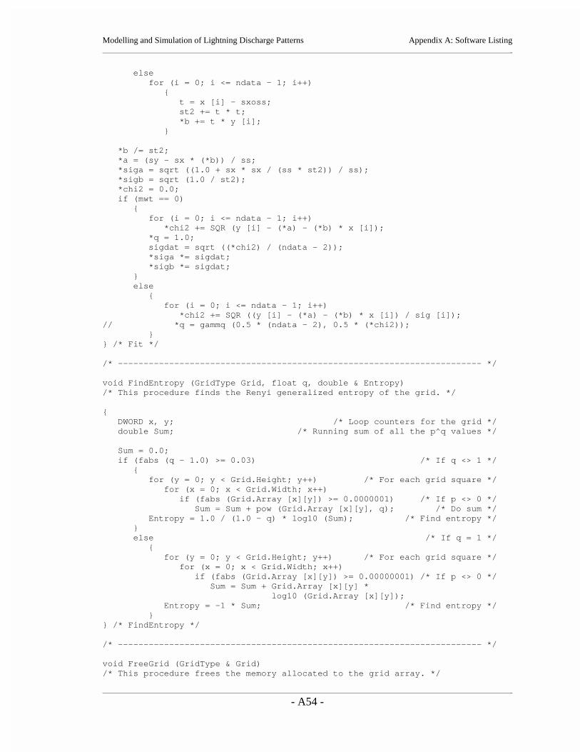
Modelling and Simulation of Lightning Discharge Patterns Appendix A: Software Listing _
_
- A54 -
else for (i = 0; i <= ndata - 1; i++) { t = x [i] - sxoss; st2 += t * t; *b += t * y [i]; }
*b /= st2; *a = (sy - sx * (*b)) / ss; *siga = sqrt ((1.0 + sx * sx / (ss * st2)) / ss); *sigb = sqrt (1.0 / st2); *chi2 = 0.0; if (mwt == 0) { for (i = 0; i <= ndata - 1; i++) *chi2 += SQR (y [i] - (*a) - (*b) * x [i]); *q = 1.0; sigdat = sqrt ((*chi2) / (ndata - 2)); *siga *= sigdat; *sigb *= sigdat; } else { for (i = 0; i <= ndata - 1; i++) *chi2 += SQR ((y [i] - (*a) - (*b) * x [i]) / sig [i]);// *q = gammq (0.5 * (ndata - 2), 0.5 * (*chi2)); }} /* Fit */
/* ----------------------------------------------------------------------- */
void FindEntropy (GridType Grid, float q, double & Entropy)/* This procedure finds the Renyi generalized entropy of the grid. */
{ DWORD x, y; /* Loop counters for the grid */ double Sum; /* Running sum of all the p^q values */
Sum = 0.0; if (fabs (q - 1.0) >= 0.03) /* If q <> 1 */ { for (y = 0; y < Grid.Height; y++) /* For each grid square */ for (x = 0; x < Grid.Width; x++) if (fabs (Grid.Array [x][y]) >= 0.0000001) /* If p <> 0 */ Sum = Sum + pow (Grid.Array [x][y], q); /* Do sum */ Entropy = 1.0 / (1.0 - q) * log10 (Sum); /* Find entropy */ } else /* If q = 1 */ { for (y = 0; y < Grid.Height; y++) /* For each grid square */ for (x = 0; x < Grid.Width; x++) if (fabs (Grid.Array [x][y]) >= 0.00000001) /* If p <> 0 */ Sum = Sum + Grid.Array [x][y] * log10 (Grid.Array [x][y]); Entropy = -1 * Sum; /* Find entropy */ }} /* FindEntropy */
/* ----------------------------------------------------------------------- */
void FreeGrid (GridType & Grid)/* This procedure frees the memory allocated to the grid array. */

Modelling and Simulation of Lightning Discharge Patterns Appendix A: Software Listing _
_
- A55 -
{ DWORD Index; /* Temporary loop counter */
for (Index = 0; Index < Grid.Width; Index++) /* For all columns */ free ((void *) Grid.Array [Index]); /* Free row memory */ free ((void *) Grid.Array); /* Free columns list */ Grid.Height = 0; /* Reset height and width */ Grid.Width = 0; Grid.Array = NULL;} /* FreeGrid */
/* ----------------------------------------------------------------------- */
void FindDq (float q, double & Dq, int Frame, GridType GridList [20])/* This procedure finds the Dq value for the grid for the current q value. */
{ double *y; /* List of entropy values */ double *x; /* List of log10 (1 / r) values */ float r; /* Current r value */ int Index; /* Loop index */ double Entropy; /* Current entropy value */// FILE *OutFile1; /* Output file for log10 (1 / r) values */// FILE *OutFile2; /* Output file for entropy values */ double a; /* y-intercept of line fit to entropy vs log10 (1 / r) graph */ double siga; /* Standard deviation of the y-intercept - unused */ double sigb; /* Standard deviation of the slope (Dq) - unused */ double chi2; /* For fitting - unused */ double GoodFit; /* For fitting - unused */
x = (double *) malloc (20 * sizeof (double)); /* Get space for lists */ y = (double *) malloc (20 * sizeof (double)); if (x == NULL || y == NULL) { printf ("Can't allocate memory in FindDq"); exit (0); } Index = 0; /* Initialize index counter */ if (fabs (q + 20.0) <= 0.00003) /* Initialize files only for q = -20 */ {// InitFile ("x", Frame, OutFile1, "w");// InitFile ("y", Frame, OutFile2, "w"); } for (r = 2; r < 256.03; r = r * 2) /* For a range of r values */ { FindEntropy (GridList [Index], q, Entropy); /* Find entropy */ x [Index] = log10 (1 / r); y [Index] = Entropy; if (fabs (q + 20.0) <= 0.00003) /* If q = -20 */ { /* Write */// fprintf (OutFile1, "%.4f ", log10 (1 / r)); /* log10(1 / r) */// fprintf (OutFile2, "%.4f ", Entropy); /* & entropy to files */ } Index++; } if (fabs (q + 20.0) <= 0.00003) /* If q = -20 */ {// fclose (OutFile1);// fclose (OutFile2); } Fit (x, y, Index, NULL, 0, & a, & Dq, & siga, & sigb, & chi2, & GoodFit); /* Fit the entropy vs. log10 (r) plot to a line with Dq as the slope */

Modelling and Simulation of Lightning Discharge Patterns Appendix A: Software Listing _
_
- A56 -
free ((void *) x); free ((void *) y);} /* FindDq */
/* ----------------------------------------------------------------------- */
void FindRenyiSpectrum (int Frame, char *DirName)/* This procedure finds the Renyi spectrum for the bmp. */
{ float q; /* Moment order */ double Dq; /* Renyi dimension value */ FILE *OutFileQ; /* Output file for q values */ FILE *OutFileDq; /* Output file for Dq values */ FILE *OutFileF; /* Output file for frame numbers */ GridType GridList [20]; /* List of grids for all r values */ float r; /* Current r value */ int Index; /* Array index for GridList */
Index = 0; for (r = 2; r < 256.03; r = r * 2) /* For a range of r values */ { GetGridProbs (GridList [Index], r, Frame, DirName); Index++; }
InitFile ("Dq", Frame, OutFileDq, "a");// InitFile ("q", Frame, OutFileQ, "w");// InitFile ("F", Frame, OutFileF, "w"); for (q = -20.0; q < 20.03; q = q + 0.2) /* For a range of q values */ { FindDq (q, Dq, Frame, GridList); /* Find Dq */// printf ("(%.2f, %.2f) ", q, Dq); fflush (stdout); fprintf (OutFileDq, "%.4f ", Dq);// fprintf (OutFileQ, "%.4f ", q); /* Write q to a file */// fprintf (OutFileF, "%d ", Frame); /* Write Frame to a file */ } fclose (OutFileDq);// fclose (OutFileQ);// fclose (OutFileF);
Index = 0; for (r = 2; r < 256.03; r = r * 2) /* For a range of r values */ { FreeGrid (GridList [Index]); /* Free grid memory */ Index++; }} /* FindRenyiSpectrum */
/* ----------------------------------------------------------------------- */
void GetDirName (char *DirName)/* This procedure reads in the directory name where the images are located. */
{ char Pref [10]; /* Temporary string for first part of file name */
printf ("Please enter the directory name and path: "); gets (DirName);
printf ("Please enter the preface of the file name: ");

Modelling and Simulation of Lightning Discharge Patterns Appendix A: Software Listing _
_
- A57 -
gets (Pref); strcat (DirName, Pref);} /* GetDirName */
/* ======================================================================= */
void main (void)
{
/* var */
int Frame; /* Current frame number */ int LowFrame; /* Low frame number to be written */ int HighFrame; /* High frame number to be written */ char DirName [256] = ""; /* Directory name entered by user */
/* main program */
GetDirName (DirName); printf ("Please enter the lower frame number: "); scanf ("%d", & LowFrame); printf ("Please enter the upper frame number: "); scanf ("%d", & HighFrame); for (Frame = LowFrame; Frame <= HighFrame; Frame++) { printf ("\nFrame %d \n", Frame); FindRenyiSpectrum (Frame, DirName); }} /* main */

Modelling and Simulation of Lightning Discharge Patterns Appendix A: Software Listing _
_
- A58 -
A.14 PlotVidDq.m
x = 1:296;y = -20:0.2:20;load Dq.txt;z = Dq;
Index3 = 1;for Index = 1:296, for Index2 = 1:201, z1(Index2,Index) = z(Index3); Index3 = Index3 + 1; end;end;
mesh (x, y, z1);view (52.5, 25);xlabel ('Frame');ylabel ('q');zlabel ('Dq');title ('Renyi Spectrum');%print -dpsc PlotDq.ps;

Modelling and Simulation of Lightning Discharge Patterns Appendix A: Software Listing _
_
- A59 -
A.15 PlotPercDq.m
x = 1:299;y = -20:0.2:20;load Dq.txt;z = Dq;
Index3 = 1;for Index = 1:299, for Index2 = 1:201, z1(Index2,Index) = z(Index3); Index3 = Index3 + 1; end;end;
mesh (x, y, z1);view (52.5, 25);xlabel ('Frame');ylabel ('q');zlabel ('Dq');title ('Renyi Spectrum');print -dpsc PlotDq.ps;