Embed Size (px)
Citation preview

EN251-0295/2012
Odemba Ian Walumasi
ECE 2304 HYDRAULICS 1
LABORATORY REPORT FOR V-NOTCH EXPERIMENT, BROAD-CRESTED WEIR
EXPERIMENT, HYDRAULIC JUMP EXPERIMENT AND SLUICE GATE EXPERIMENT.
By ODEMBA IAN WALUMASI
EN251-0295/2012
Supervised by Dr. Kazungu Maitaria
As part of fulfillment towards the award of Bachelor in Science degree in
CIVIL ENGINEERING from
DEPARTMENT OF CIVIL, CONSTRUCTION AND ENVIRONMENTAL ENGINEERING,
COLLEGE OF ENGINEERING AND TECHNOLOGY,
JOMO KENYATTA UNIVERSITY OF AGRICULTURE AND TECHNOLOGY.
THIRD YEAR, FIRST SEMESTER
2014/2015 Academic Year
December 2014

EN251-0295/2012
Odemba Ian Walumasi
EXPERIMENT OF THE V-NOTCH
ABSTRACT
The following is a detailed report on the V-notch. Hydraulic structures are devices used to
regulate or measure flow in an open channel, useful for purposes of distribution, management
and use of flowing water. The V-Notch weir is a type of hydraulic structure called a sharp-crested
weir used to measure or regulate volumetric flow in open channel hydraulics. The experiment of
the V-notch (triangular sharp-crested weir), was conducted under the condition of uniform flow.
Data was collected with values of head for flow and actual discharge being observed. Using
standard equations values for theoretical discharge and coefficient of discharge could be
determined. The main purpose of the V-notch experiment is to compare actual discharge and
theoretical discharge and therefore calibrate the V-notch to measure discharge.
INTRODUCTION
Background Information
In open channel flows the knowledge of discharge is important in order to solve simple open flow
equations. A sharp crested (thin plate) weir is a restrictive plate placed vertically across the whole
span of an open channel raising upstream water level enabling measurement of discharge.
Various geometries and sizes can thus be used on the thin plate depending on the precise
application of the weir.
The weir under consideration in this case is the V-notch also known as the triangular/v-shaped
sharp crested weir. The V-notch has advantage over the rectangular shaped thin plate because
the shape of the nappe does not change with head so the coefficient of discharge does not vary
so much. The V-notch controls flow such that water head must reach a given head before flow
occurs over it. It also serves as a discharge measurement device as the head upstream increases
the discharge across the V-notch also increases thus discharge can be determined by measuring
the head upstream.
Knowledge in Relation to Experiment
1. Theoretical discharge (Qt) is given by:
Qt = 8/15 (√2g) H5/2 tan Ѳ = K’ H5/2 …… eq.1
Where g = gravitation acceleration.
H = head above notch. Ѳ = half angle of notch.
K’ = 8/15(√2g) tan Ѳ.
However in the experiment Ѳ = 45˚; thus tan 45˚ = 1.

EN251-0295/2012
Odemba Ian Walumasi
2. Coefficient of discharge (Cd) is given by:
Cd = Qa / Qt …… eq.2
Where Qa represents the actual discharge obtained by the discharge measurement device (gravimetric method)
3. Conversion of the head into the real discharge:
Qa = Cd * Qt = 8/15 Cd (√2g) H5/2 = Cd K’ H5/2 …… eq.3
Replacing 8/15 Cd (√2g) by K:
Qa = KH5/2 …… eq.4
In the experiment, Qa and H are measured. K can be obtained from the following equation:
K = Qa / H5/2 …… eq.5
When logarithmic scale paper is applied to eq.4 K is determined based on an H-Q graph. Applying the logarithmic operation to eq.4:
Log Qa = log K + 5/2 log H …… eq.6
Therefore, when the experimental data are joined by a straight line with a gradient of 5/2 the actual discharge corresponding H = 1 m gives the value of K.
4. Formulae according to the British Standards (BS 3680, part 4A);
According to the BS 3680 part 4A the discharge equation for a V-notch with the angle between 20o and the 100o is as:
Qa = 8/15 CB (√2g) HB5/2 tan Ѳ …… eq.7
Where: CB = coefficient of discharge varying with the value of Z/B and H/Z as
shown in fig.3, and HB= head which allows for the effects of viscosity and surface
tension.
Using kh for effects:
HB = h + kh …… eq.8
Using kh is the constant value of 0.00085m for a corresponding range of values of
H/Z and H/B in fig.3 since K is very small, it is neglected in the experiment.

EN251-0295/2012
Odemba Ian Walumasi
Relationship between CB and H/Z (fig.3)
The objectives of the V-notch experiment
a) To observe the state of flow through a V-notch.
b) To determine the relationship between the discharge and the head above the notch.
c) To compare theoretical discharge and the actual discharge.
d) To compare the coefficient of discharge obtained with BS requirements.
For the experiment of the V-notch, the head upstream of the V-notch is expected to increase with
increase in discharge after condition of steady uniform flow is established. The relationship between the
theoretical and actual discharge gives the coefficient of discharge for the V-notch.
MATERIALS AND METHODS
Apparatus (Materials)
1. A steady water supply system
2. An approach channel with a hook gauge
3. A sharp- edged V-notch
4. A discharge measurement device (a bucket, steel container and a weighing balance)
5. Stopwatch
6. Thermometer

EN251-0295/2012
Odemba Ian Walumasi
Set up of the experiment (fig. 1)
Details of V-notch plate and baffle (fig.2)

EN251-0295/2012
Odemba Ian Walumasi
Procedure (Method)
1. The width of the approach channel and the height of the crest were measured with a steel
tape.
2. The temperature of the water was taken.
3. The crest level of the V-notch was measured using a hook gauge. It was taken after the
approach channel was filled up to the crest with water.
4. The operation was started with a steady water supply and a small discharge set with the
gate valve.
5. After the water became steady, the water level was measured with a hook gauge
6. The discharge was measured with a bucket and a weighing balance.
7. The discharge was increased a little and procedures 5and 6 repeated. A steel container
was used instead of a bucket when the discharge became so large.
RESULTS
The following requirements were met for presentation of the results for the experiment of the
V-notch;
1) Sketching a flow over V-notch (choose one flow). Especially the experimenter should
observe the contraction of flow.
2) Preparing an arrangement table (table 2) and filling in the columns with the data.
3) Calculating the following values and filling up the table (table2);
a) Constant value of V-notch (K´)
b) Actual discharge (Qa)
c) Theoretical discharge (Qt)
d) Coefficients of discharge for each stage (Cd)
e) Coefficient for each stage (K)
4) Plotting the head (H) on abscissa and the actual discharge (Qa) on ordinate on the log-log
graph and drawing the equality: Qt = K’ H5/2.
5) Finding the mean value of the coefficient of discharge and the mean value of the coefficient,
casting aside doubtful data.
6) Plotting the theoretical discharge (Qt) on abscissa and the actual discharge (Qa) on ordinate
on part paper.
7) Plotting the coefficient of discharge (Cd) on abscissa and on ordinate on section paper.

EN251-0295/2012
Odemba Ian Walumasi
Sketch of flow over the V-notch (fig.4)
The flow over the V-notch was observed to have a
free nappe before data was collected.
Data Sheet
Fundamental data (table1)
PROPERTIES OF WATER Temperature (˚C) 21
Density (ρ)(Kg/m3) 1000
MASS OF BUCKET (Kg) 0.6
PROPERTIES OF V-NOTCH Width of channel (B) (m) 0.6
Height of crest (m) 0.12
Half angle of notch (Z) (degrees) 45
K’ ( = 8/15(√2g) tan Ѳ) 2.3624
Crest level reading (m) 0.2205

EN251-0295/2012
Odemba Ian Walumasi
Operation Data and Calculated values (table2) st
age
Actual Discharge Manometer
H/Z
theo
reti
cal d
isch
arge
( *
10
3m
3/s
)
Cd
K to
tal m
ass
(Kg)
mas
s o
f w
ater
(K
g)
volu
me
( *1
03 m
3)
tim
e (s
ec)
dis
char
ge (
* 1
03 m
3/s
)
mea
n d
isch
arge
( *
10
-3 m
3/s
)
read
ing
(m)
hea
d (
H)
(m)
1 6.5 5.9 5.9 3.54 1.67 1.64 0.158 0.0625 0.5208 2.31 0.71 1.677
11.1 10.5 10.5 6.41 1.64
9.2 8.6 8.6 5.33 1.61
2 9.9 9.3 9.3 4.67 1.99 2.00 0.15 0.0701 0.5842 3.07 0.65 1.539
10.6 10.0 10.0 5.19 1.93
11.0 10.4 10.4 4.97 2.09
3 10.7 10.1 10.1 4.14 2.44 2.43 0.145 0.0755 0.6292 3.70 0.66 1.552
12.3 11.7 11.7 4.93 2.37
9.5 8.9 8.9 3.58 2.49
4 10.5 9.9 9.9 3.23 3.07 2.96 0.136 0.0844 0.7033 4.89 0.61 1.43
10.2 9.6 9.6 3.30 2.91
11.6 11.0 11.0 3.79 2.9
5 13.1 12.5 12.5 3.53 3.54 3.57 0.132 0.0886 0.7217 5.52 0.65 1.528
12.7 12.1 12.1 3.32 3.64
12.6 12.0 12.0 3.39 3.54
6 13.4 12.8 12.8 3.17 4.04 4.15 0.126 0.0945 0.7875 6.49 0.64 1.511
9.2 8.6 8.6 2.09 4.11
10.5 9.9 9.9 2.31 4.29
Mean values Cdm =
0.65
Km =
1.5400
The following graphs were drawn from the data acquired and computed

EN251-0295/2012
Odemba Ian Walumasi
Graph 1: Discharge against head on section graph
Graph 2: Discharge against Head on log-log graph
1.642
2.43
2.96
3.57
4.15
2.31
3.07
3.7
4.89
5.52
6.49
0
1
2
3
4
5
6
7
0.05 0.055 0.06 0.065 0.07 0.075 0.08 0.085 0.09 0.095 0.1
Dis
char
ge (
*10
-3m
3/s
)
Head (H) (m)
Discharge against Head
Actual discharge against HeadTheoretical discharge against Head
0.1
1
1
Log
Q(D
isch
arge
)
Log H(Head)
Log Q against Log H
log Qa against Log H Log Qt against Log H
Linear (log Qa against Log H) Linear (Log Qt against Log H)

EN251-0295/2012
Odemba Ian Walumasi
Graph 3: Actual discharge against theoretical discharge on section graph
Graph 4: H/Z against Coefficient of discharge (Cd)
y = 0.6024x + 0.1832
0
1
2
3
4
5
6Q
a(*1
0-3
m3/s
)
Qt(*10-3m3/s)
Qa against Qt
Qa against Qt Linear (Qa against Qt)
0.5208
0.5842
0.6292
0.70330.7217
0.7875
0.4
0.45
0.5
0.55
0.6
0.65
0.7
0.75
0.8
0.85
0.6 0.62 0.64 0.66 0.68 0.7 0.72
H/Z
Cd
H/Z against Cd
H/Z against Cd

EN251-0295/2012
Odemba Ian Walumasi
DISCUSSION
The following considerations were made for the discussion
1. Deriving Eq.1 from the continuity equation and Bernoulli’s equation;
Consider a small elemental strip of flow across the V-notch with thickness dh and breadth b, as
shown in fig.5 below.
The width of the strip changes with depth such that
b = 2(H - h) tan (Ѳ/2)
Q = 0 ʃ H u.bdh = 2(√2g) tan (Ѳ/2) 0 ʃ H (H - h) h1/2 dh
Q = 2(√2g) tan (Ѳ/2) 0 ʃ H (Hh1/2 - h3/2) dh
Q = 2(√2g) tan (Ѳ/2) [2/3 H5/2 – 2/5H5/2]
Q = 2(√2g) tan (Ѳ/2) [4/15H5/2]
Thus theoretical discharge is given by: Qt = 8/15 (√2g) H5/2 tan (Ѳ/2) …… (eq.9)
Comparing eq.9 to eq.1; Ѳ/2 = Ѳ, thus Qt = 8/15 (√2g) H5/2 tan Ѳ …… (eq.1)
2) Explaining why the actual discharge is smaller than the theoretical discharge. And stating the
significance of the coefficient of discharge;
The value of actual discharge is smaller than the theoretical discharge due to head losses. These
head losses include:
Head losses due to friction. This is the main cause of head losses in the V-notch
experiment.
Head losses due to contraction due to the geometry of the V-notch.
Head losses due to variation of pressure and velocity with the V-notch being a barrier to
flow.

EN251-0295/2012
Odemba Ian Walumasi
The coefficient of discharge enables the determination of actual discharge from theoretical
discharge and thus enabling a calibrated V-notch (whose Cd has been established) to be used
for measurement of actual discharge.
3) Inquiring on sources of error;
Possible sources of error include errors in observing readings for examples observing and
recording mass, time and head readings. Errors may also originate from fluctuations in
temperature which vary the properties of water.
4) Comparing fig.3 and the figure of Graph 4 and describing the accuracy of the experimental
data;
The shape obtained on Graph 4 is polynomial in nature compared to the exponential curves on
fig.3.However, if similarly plotted the polynomial graph is somewhat similar to what would have
been obtained; given the value of Z/B = 0.2, therefore the V-notch experiment was acceptably
precise in calibration of the V-notch.
5) Explaining why the edge of the notch is sharpened at 45°;
The edge of the notch is sharpened to reduce drag on flow as a flat surface increases resistance
to flow causing formation of eddies thus causing drag and also it limits formation of a free nappe.
CONCLUSION
As seen from the comparison between the graphs obtained from the experiment with the
expected graphs from British Standards, the experiment was successful in the calibration of the
V-notch with a Cdm value of 0.65 being obtained. Values for theoretical and actual discharge were
successfully obtained thereby fulfilling all the objectives of the experiment.
CITED LITERATURE
Lecture notes
Manual for Hydraulics and Water resources JKUAT, School of Civil Construction and
Environmental Engineering
ECE2304 Hydraulic Structures, Dr. Kazungu Maitaria, Civil Engineering Department
JKUAT.
Hydrology Tutorial- Flow in Open Channels,www.freestudy.co.uk

EN251-0295/2012
Odemba Ian Walumasi
EXPERIMENT OF THE BROAD - CRESTED WEIR
ABSTRACT
In contrast to plate weirs long- based weirs are larger and generally more heavily constructed.
The broad crested (rectangular) weir is a type of long-based weir used in measurement of
discharge. They are usually designed for use in the field and are thus usually subject to large
discharges. The broad crested weir acts an obstacle to flow and thus applying the principle of
conservation of energy, the depth and velocity of flow at weir can be determined for a given
discharge, depending on the nature of discharge. The broad crested weir can thus be calibrated
for measurement of discharge. In the experiment of the broad crested weir, the weir was set to
give a condition of critical flow thus flow over the weir was critical flow (specific energy =
minimum). The following is detailed description of the experimental procedure, presentation
and analysis of the results and a final conclusion of the analysis for the broad-crested weir.
INTRODUCTION
Basic Information
When an obstacle is introduced to a uniform open channel flow system, there is a drop in the
specific energy (see fig.1, fig.2). The change in depth varies according the type of flow
upstream. If the flow is subcritical, and the height of the obstacle (Z) is small in comparison to
the depth of flow upstream (y1), then the depth of flow at the obstacle (y2) is smaller than the
depth upstream as shown in fig.2. If the flow is supercritical, and the height of the obstacle (Z)
is small in comparison to the depth of flow upstream (y1), then the depth of flow at the
obstacle (y2) is greater than the depth upstream.
Effect of an obstacle to open channel uniform flow (fig.1)

EN251-0295/2012
Odemba Ian Walumasi
Effect of obstacle on the specific energy and depth of flow (fig.2)
However when the height of the obstacle is great in comparison to the depth of flow upstream,
for a specific discharge, there is a given height (Zc) that causes the flow over the barrier to be
critical, as shown in fig.2. A further increase in the height of the obstacle does not change the
state of flow and thus the depth of flow over the barrier is critical depth (yc). The broad crested
weir under consideration was pre-conditioned to create critical flow condition. The channel
lining and slope which affect velocity of flow as per manning’s equation can be shown to have
the following effect on the critical flow depth for a rectangular broad-crested weir. Where ξ =
√(S)/η, S = Slope of channel, η = manning’s roughness coefficient (fig.3)
Variation of critical depth with channel conditions (fig.3)

EN251-0295/2012
Odemba Ian Walumasi
Knowledge in Relation to the Experiment
1. Actual Discharge;
In this experiment, the actual discharge (Qa) is measured by the V-notch. It is given as follows:
…… eq.1
…… eq.2
Where HV = Head above the V-notch.
Cdv = Coefficient of discharge of V-notch.
Ѳ = Half angle of V-notch.
KV = Coefficient of V-notch.
The values of Cd and KV been obtained in the previous V- notch experiment.
2. Specific Energy;
The total head reckoned from the crest level of the broad crested weir at section 1 (E) is as:
……eq.3
Where H1 = depth at section 1.
Z = height of the weir.
V1 = velocity of flow at section 1 (approaching velocity).
B = width of weir.
The specific energy at the weir is equal to the total head (E).
There is a relationship between the specific energy (E) and the depth at the control section
(critical depth, HC) as follows:
…… eq.4
If the critical depth is measured, it is very easy to calculate the specific energy and the discharge
over the weir. However, it is difficult to find out the critical section.

EN251-0295/2012
Odemba Ian Walumasi
In this experiment, to determine the coefficient of discharge of the broad crested weir, the
upstream depth and the approaching velocity which is calculated as Qa/ (BH1) are adopted.
3. Discharge Equation;
The theoretical discharge over a broad crested weir (Qt) is given as:
…… eq.5
The coefficient of discharge (Cd) is found as the ratio of the actual discharge (Qa) to the
theoretical discharge (Qt):
…… eq.6
According to the British Standards (BS 3680, PART 4F), the coefficient of discharge is
theoretically given as:
……eq.7
Where Cdt = theoretical coefficient of discharge.
L = length of flat portion of the weir.
Actually in the field it is important to find the relationship between the depth at section 1 (H1)
and the actual discharge (Qa) since the water level is measured in a gauge well-constructed in
the upstream of the weir.
4. Froude Number;
When the actual discharge (Qa) and the depth (H) are known he Froude number (Fr) is
calculated as follows:
…… eq.8

EN251-0295/2012
Odemba Ian Walumasi
……eq.9
The flows are classified into 3 states according to Froude number
i. Fr < 1.0: subcritical flow
ii. Fr = 1.0: critical flow
iii. Fr > 1.0: subcritical flow
The following assumptions were made during the experiment;
The flow falls freely over the weir such that a free nappe occurs and that there is no
external interference to the rate of flow of water.
The streamlines above the weir are horizontal, for easier collection and computation of
data.
There are absolutely no energy and head losses. Energy losses in form of noise, friction
losses and internal energy losses are taken to be negligible.
The velocity approach over the weir is also taken to be uniform and parallel to the
channel floor.
Objectives of the experiment
1) To observe the change of the state of flow.
2) To calibrate a laboratory -scale round nose broad-crested weir.
3) To compare the coefficient of discharge obtained by the experiment with that by the
British Standard (BS 3680, Part 4F).
MATERIALS AND METHODS
Apparatus (materials)
1) A round -nose broad crested weir with rubber packings
2) A steady water supply system
3) An adjustable -slope rectangular open channel with point gauges
4) A v-notch with a hook gauge
5) A steel tape measure
6) A thermometer

EN251-0295/2012
Odemba Ian Walumasi
Set up of experiment apparatus (fig.4)
Detail of broad-crested weir (fig.5)

EN251-0295/2012
Odemba Ian Walumasi
Procedure (method)
1) The dimensions of the broad- crested weir were measured and the distance from
section 2A to 2B - section 2F taken.
2) The open channel horizontal was set horizontal.
3) The temperature of the water was measured.
4) The crest level of the broad- crested weir and the level of the channel bed were
measured with the point gauge.
5) The crest level of the v-notch was measured with the hook gauge, pouring the water up
to the crest level.
6) The operation of the steady water supply system was started and the discharge set to
be small.
7) The head above the v-notch was measured after the flow become steady.
8) The depth of the flow in the upstream where the weir does not exert influence on the
water surface (section 1) was measured
9) The change of the state of flow by the broad- crested weir was observed and the section
where the control section occurs was established, letting a drop of water fall on the
surface of flow.
10) The discharge was increased a little and procedure 7 and 8 repeated.
11) One flow was selected and the depths of flow at section 2A-section 2F measured.
RESULTS
The following requirements were met for presentation of the results;
1) Sketching a flow over the broad-crested weir (choose one flow) (see fig.6).
2) Preparing arrangement tables (table 1, 2, 3 and 4) and filling in the columns with the data.
3) Calculating the following values and fill in the table 2;
a) Actual discharge (Qa)
b) Approaching velocity
c) Velocity head (V12/2g)
d) Specific energy (E)
e) Theoretical discharge (Qt)
f) Coefficient of discharge ( Cd)
g) Value of L/(H1-Z)
h) Theoretical coefficient of discharge ( Cdt)
4) Plotting the specific energy (E) on the abscissa and the actual discharge (Qa) on ordinate on
log-log graph, and drawing eq.5.

EN251-0295/2012
Odemba Ian Walumasi
5) Finding the mean value of the coefficient of discharge (Cdm) after setting aside doubtful data,
on referring to the graph completed in step (4).
6) Plotting the upstream depth (H1) on abscissa and the actual discharge (Qa) on ordinate on
section paper and draw the equality Qt= 1.705B (H1-Z) in which the approaching velocity is
neglected.
7) Plot H1 on abscissa and the coefficient of discharge (Cd) on the ordinate on the section graph
on which the graph of eq.7 had been already shown.
8) Calculating the following values for section 2A-section 2F and fill the table 2
1) Velocities of flow (V2A, V2B ……V2F).
2) Propagation velocities of long waves (U2A, U2B……U2F).
3) Froude numbers (Fr2A, Fr2B…… Fr2F).
9) Drawing the profile of flow over the weir, plotting the data of the depths at section 2A to
section 2F, and presuming the location of the control section
Data Sheet I
Fundamental data I (table 1)
Properties of water Temperature 21 °C
Density (ρ) 1000 Kg/m3
Dimension of Broad- Crested weir
Width (B) 0.30m
Length (L) 0.30m
Height (Z) 0.15m
1 – {(0.006L) /B} 0.994
Crest level (point gauge) 0.626m
Property of channel Bed level (point gauge) 0.476
Half angle of v-notch 45 °
Coefficient of discharge (Cdv) 0.65
Coefficient (KV) 1.5355
Crest level (hook gauge) 0.2193m

EN251-0295/2012
Odemba Ian Walumasi
Operation data I (table 2)
Stag
e
V-notch Section 1
(H1 –
Z)
(m)
L/ (
H1 -
Z)
Specific Energy
Theo
reti
cal d
isch
arge
(*
10-3
m3 /
s)
Cd
Cdt Rea
din
g (m
)
Hea
d (
HV)
(m)
Dis
char
ge (
Qa)
(*1
0-3
m3 /
s)
Rea
din
g (m
)
Dep
th (
H1)
(m)
Vel
oci
ty o
f fl
ow
(V1)
(*1
0-3 m
/s)
Vel
oci
ty H
ead
(V
12 /
2g)
(*1
0-6
m)
Spec
ific
en
ergy
(E)
(m
)
1 0.1450
0.0743
2.311
0.652
0.176
0.026
11.5
43.77
97.65 0.02609
2.149
1.075
0.9428
2 0.1446
0.0747
2.342
0.652
0.176
0.026
11.5
44.36
100.3 0.02610
2.15 1.089
0.9428
3 0.1416
0.0777
2.584
0.654
0.178
0.028
10.7
48.39
119.35
0.02812
2.405
1.074
0.9465
4 0.1359
0.0834
3.084
0.657
0.181
0.031
9.68
56.80
164.44
0.03116
2.805
1.099
0.9510
5 0.1259
0.0934
4.094
0.663
0.187
0.037
8.11
72.98
271.46
0.03727
3.67 1.116
0.9580
6 0.1202
0.0991
4.747
0.667
0.191
0.041
7.32
82.84
349.77
0.04135
4.284
1.108
0.9614
7 0.1136
0.1057
5.578
0.672
0.196
0.046
6.52
94.86
458.64
0.04646
5.107
1.092
0.9650
8 0.1013
0.1180
7.344
0.680
0.204
0.054
5.56
120.00
733.94
0.05473
6.530
1.125
0.9693
9 0.0908
0.1285
9.089
0.688
0.212
0.062
4.84
142.90
1040.80
0.06304
8.072
1.126
0.9724
10 0.0701
0.1492
13.200
0.705
0.229
0.079
3.80
192.14
1881.64
0.08088
11.70
1.128
0.9771
Mean values Cdm
= 1.103
Cdtm =
0.9586

EN251-0295/2012
Odemba Ian Walumasi
The following graphs were drawn;
Graph 1: Log Qa against Log E
Graph 2: Theoretical discharge against (H1-Z)
0.1
1
1
Log
Qa(
Act
ual
dis
char
ge)
Log E(Specific energy)
Log Qa against Log E
Log Qa against Lof E Linear (Log Qa against Lof E)
y = 0.5093x + 4E-050
2
4
6
8
10
12
14
16
0 0.01 0.02 0.03 0.04 0.05 0.06 0.07 0.08 0.09
Theo
reti
cal d
isch
arge
(*1
0-3
m3
/s)
(H1-Z) (m)
Theoretical discharge against (H1-Z)
Qt against (H1-Z) Q' t against (H1-Z)
Expon. (Qt against (H1-Z)) Linear (Q' t against (H1-Z))

EN251-0295/2012
Odemba Ian Walumasi
Graph 3: Coefficient of Discharge (Cd) against Depth of flow upstream (H1)
Data sheet II
Fundamental data II (table 3)
Selected stage Stage 10
Actual discharge Qa 13.2 * 10-3 m3/s
Crest level of weir 0.626m
Width of the weir (B) 0.30m
Operational data II (table 4)
section Distance from 2A (m)
Water level (point gauge)
Depth (H)(m)
Velocity of flow (v) (m/s)
Propagation velocity (u) (m/s)
Froude number (Fr)
2A 0.0 0.696 0.070 0.629 0.829 0.7587
2B 0.05 0.686 0.060 0.730 0.767 0.9518
2C 0.10 0.679 0.053 0.830 0.721 1.1512
2D 0.15 0.675 0.049 0.898 0.693 1.2958
2E 0.20 0.671 0.045 0.978 0.664 1.4729
2F 0.25 0.659 0.033 1.333 0.569 2.3427
0.8
0.85
0.9
0.95
1
1.05
1.1
1.15
1.2
0 0.05 0.1 0.15 0.2 0.25
Cd
(co
effi
cien
t o
f d
isch
rage
)
H1(Depth of flow upstream)
Cd against H1
Cd against H1 Log. (Cd against H1)

EN251-0295/2012
Odemba Ian Walumasi
DISCUSSION
The following considerations were made for discussion and analysis;
1) Given the critical depth is 2.00cm, finding the discharge by applying the mean coefficient of
discharge (Cdm):
Q = Cdm * 1.70 * B * E3/2 but E = 3/2HC
Q = 1.103 * 1.70 * 0.3 * 3/2(0.02)3/2
Q = 0.0029m3/s
2) Stating the facts discovered in the graph completed above:
For the broad-crested weir under consideration, critical flow occurs when Froude’s number
(Fr) = 1. This occurs between section 2B and 2C. Critical depth is approximately 0.057m for Q =
13.2 * 10-3 m3/s. The weir has rounded edges to reduce drag to flow and head losses. The
change in the type of flow is as shown in the fig.6 below:
Sketch of flow profile over the broad-crested weir (fig.6)
3) Stating the relationship between upstream depth (H1) and the discharge.
Graph 2 shows the relationship between theoretical discharge and depth of flow above the
crest of the broad-crested weir described by an exponential graph trend. The relationship
between actual discharge and depth of flow upstream(H1) follows the same exponential trend
with discharge increasing exponentially with increase in depth of flow given that actual
discharge is given by (see eq.5 and eq.6):
Qa = Cd * 1.70 * B * {(H1 – Z) + 1/2g (Qa/B.H1)2}3/2 …… eq.10
Where Cd = coefficient of discharge of weir
H1 = depth of flow upstream
B = Internal breadth of rectangular-section channel

EN251-0295/2012
Odemba Ian Walumasi
Possible sources of Errors 1. Error in observing hook gauge and point gauge readings 2. Large head and energy losses occurring. 3. Errors in calibration affecting the reliability of the characteristic discharge coefficient (Cd) CONCLUSION The experiment was successful as the objectives of the experiment were met. The critical depth was established to be approximately 0.057m The flow over the broad-crested weir was observed (fig.6), the broad-crested weir was calibrated (Cdm = 1.103), and flow compared to British Standards with graphs from experimental and computed data drawn. CITED WORK
Lecture notes
Manual for Hydraulics and Water resources JKUAT, School of Civil Construction and
Environmental Engineering
ECE2304 Hydraulic Structures, Dr. Kazungu Maitaria, Civil Engineering Department
JKUAT.
Civil Engineering hydraulics(Essential Theory and Worked Examples), R.E. Featherstone
and C. Nalluri, Third Edition 1998

EN251-0295/2012
Odemba Ian Walumasi
EXPERIMENT OF THE HYDRAULIC JUMP
ABSTRACT
Hydraulic jump is a phenomenon in open channels commonly observed when a supercritical
flow meets a subcritical flow, resulting in transitional rapid flow which involves a substantial
amount of energy loss. The hydraulic jump experiment was conducted in a laboratory to aid in
analysis of a hydraulic jump. This includes determination of specific energy for the hydraulic
jump and application of the momentum equation in determining the energy losses in the
hydraulic jump. The hydraulic jump is a significant structure in open channel hydraulics with the
following applications:
Dissipation of energy of water flowing over dams and weirs – to prevent possible
erosion and scouring due to high velocities
Raising water levels in canals to enhance irrigation practices and reduce pumping heads
Reducing uplift pressure under the foundations of hydraulic structures
Creating special flow conditions to meet certain special needs at control sections such as
gaging stations, flow measurement and flow regulation
INTRODUCTION
Basic Theory
A hydraulic jump occurs when water in an open channel is flowing supercritical and is slowed by
a deepening of the channel or obstruction in the channel causing the water surface to rises
abruptly, and changing into subcritical flow with considerable to large energy loss. There are
several types of hydraulic jumps
a) Undular jump (1.0 <Fr1 <1.7): The jump exhibits slight undulation. The conjugate
depths of the jump are close and transition is less abrupt with slightly ruffled water.
b) Weak jump (1.7 <Fr1 <2.5): There is formation of eddies and rollers at the surface of
the jump, with small energy loss. The ratio of final depth to initial depth is between
2.0 and 3.1. The velocity throughout is fairly uniform, and the energy loss is low.
c) Oscillating jump (2.5 <Fr1 <4.5): A jet oscillates from top to bottom generating
surface waves that persist beyond the end of the jump. The ratio of final depth to
initial depth is 3.1 to 5.0.
d) Stable/Steady jump (4.5 <Fr1 <9.0): The downstream extremity of the surface
roller and the point at which the high velocity jet tends to leave the flow occur at
practically the same vertical section. The energy dissipation ranges from 45 to 70%.
e) Strong /Rough jump (Fr1 >9.0): The high-velocity jet grabs intermittent slugs of water
rolling down the front face of the jump, generating waves downstream, and a rough
surface can prevail. The jump action is rough but effective since the energy
dissipation may reach 85%.

EN251-0295/2012
Odemba Ian Walumasi
A hydraulic jump may occur in the following conditions
1) When a steep slope flow encounters a mild slope flow. The sequent depth can be
compared to normal depth of flow over the mild slope.
2) When flow transitions from a steep slope to an adverse slope (sloping in an opposite
direction). This a complicated case and the jump may occur on either slope.
3) Due to change in profile caused by a sluice gate. A hydraulic jump may occur upstream
(for a steep slope) or downstream (for a gentle slope) of the sluice gate.
Specific energy of a hydraulic jump (fig.1)
Consider the hydraulic jump as shown in fig.1 above
The specific energy at the initial depth (H1) is given by E1 = h1 + v12/ 2g
The specific energy at the sequent depth (H2) is given by E2 = h2 + v22/ 2g
However when projected using equivalent specific energy of the initial depth, the depth
expected (alternate depth) is greater than the depth observed during the hydraulic jump
(sequent depth). Therefore as seen in fig.1, E1 > E2 there is energy loss during the hydraulic
jump (ΔE).
Considering fig.1 above where for the respective sections 1 and 2: h1, h2 = depths of flow, V1, V2
= mean velocity of flow, Fr1, Fr2 = Froude’s number, Q = discharge and b = Breadth of
rectangular section;

EN251-0295/2012
Odemba Ian Walumasi
The loss of energy head due to the occurrence of the hydraulic jump is the difference between
the specific-energy heads at sections:
ΔES = ES1 – ES2 = (h1 + v12/ 2g) - (h2 + v2
2/ 2g)
ΔES = (h1 – h2) {(v12 - v2
2)/ 2g} …… eq.1
But q = v/h where q = mass flux for a rectangular section channel q = Q/b
ΔES = (h1 – h2) {q2 (h22 – h1
2)}/ (2g.h12h2
2) (1)
However q2/2g.h1h2 = (h1 + h2)/2 therefore:
ΔES = (h1 – h2) {(h1 + h2)/4h1h2} * (h22 – h1
2) (2)
ΔES = 1/4h1h2 {3h12h2 – 3h1h2
2 + h23 – h1
3} (3)
ΔES = (h2 – h1)3 / 4h1h2 …… eq.2
Due to these head losses and internal energy losses the principle of conservation of energy
cannot be used in the analysis of the hydraulic jump and as a result, the principle of
conservation of momentum is used in the analysis of a hydraulic jump. In this case Newton’s
second law of motion is employed.
Consider fig.2 below where for the respective sections 1 and 2: h1, h2 = depths of flow, F1, F2 =
force at section, P1, P2 = Hydrostatic pressure, V1, V2 = mean velocity of flow, Fr1, Fr2 = Froude’s
number, q = mass flux (mass per second) and b = Breadth of rectangular section.
Analysis of a hydraulic jump (fig.2)
In the flow direction;

EN251-0295/2012
Odemba Ian Walumasi
Force F1 = ρgh1 (h1/2) from P1 and F2 = ρgh2 (h2/2) from P2
The net force (F1 - F2) is equivalent to the change in hydrostatic pressure force from P1- P2
given by:
F1 – F2 = ρg {h12/2) – h2
2/2)} But w (specific weight) = ρg, thus
F1 – F2 = w {h12/2) – h2
2/2)} …… eq.3
Change in momentum (M1 – M2) is given by
M1 – M2 = (𝒘𝒒/g) (v1 – v2) where g = gravitational acceleration, q = mass flux
However we know from continuity v = q/h thus replacing for v1 and v2;
M1 – M2 = (wq/g) {(q/h2) - (q/h1)}
M1 – M2 = (wq2/g) {(h1 – h2)/h1h2} …… eq.4
We Know from Newton’s second law of motion that the change in momentum is equal to the
force acting at a given point thus equating eq.1 and eq.2
F1 – F2 = M1 – M2 (1)
w {h12/2) – h2
2/2)} = (wq2/g) {(h1 – h2)/h1h2} (2)
1/2 (h12 – h2
2) = q2/g (h1 – h2)/h1h2 (3)
(h12 – h2
2) = 2q2/g (h1 – h2)/h1h2 (4)
(h1 + h2) (h1 – h2) = (2q2/g.h1h2) (h1 - h2) (5)
h1 + h2 = 2q2/g.h1h2 (6)
h22 + h1h2 = (2q2/g.h1) (7)
h22 + h1h2 - (2q2/g.h1) = 0 …… eq.5
Solving the quadratic equation above for h2 and ignoring the negative result
h2 = -h1 /2 + [h12/4 – 2q2/g.h1]1/2
However 2q2/g.h1 = 2Fr12h1
2 thus;
h2 = -h1 /2 + h1 {[1/4 + 2Fr1] 1/2 – 1/2}
Multiplying with 2
h2 = h1/2 {(1 + 8Fr1)1/2 - 1} …… eq.6

EN251-0295/2012
Odemba Ian Walumasi
Knowledge with respect to the experiment
1) Actual discharge;
In this experiment, the actual discharge (Qa) is measured by the v-notch .It is given as follows:
……eq.7
Where HV=head above V-notch.
Cdv = Coefficient of discharge of V-notch
Ѳ = half angle of v-notch
KV = coefficient of discharge
The values of Cdv and KV have been obtained in experiment on the v-notch
(2) Specific energy;
Since the channel s horizontal the specific energy (E) is given by:
……eq.8
Where H = depth of flow.
α = Energy coefficient (= 1.0 to 1.1 in laboratory).
V = mean velocity of flow.
B = breadth of rectangular channel.
3) State of flow;
Based on fig.3, the flow with a certain value of specific energy (E) can form two types of flow:
subcritical flow with larger flow depth (Hsp) and supercritical flow with smaller flow depth (Hsp).
When specific energy equal Ec, the flow becomes critical. We know that critical flow occurs over
the broad crested weir and critical mean velocity is given by:
……eq.9
Where HC represents critical flow depth

EN251-0295/2012
Odemba Ian Walumasi
Depth (H) against specific energy (E) for constant discharge (fig.3)
Froude’s number is calculated in order to classify flow. The table 1 below shows the
relationship between the Froude’s number and state of flow.
Relationship between Froude’s number and state of flow (table 1)
Velocity of flow
Depth of flow
Propagation of wave velocity (u)
Froude’s number
Subcritical Vsb Hsb √(g.Hsb) Fr = Vsb/√(g.Hsb) < 1.0
Critical Vc Hc √(g.Hc) Fr = Vc/√(g.Hc) = 1.0
Supercritical Vsp Hsp √(g.Hsp) Fr = Vsp/√(g.Hsp) > 1.0
4) Change in depth due to hydraulic jump;
The relationship between the depth upstream of the hydraulic jump (H1) and downstream of
the hydraulic jump (H2) is:
…… eq.10

EN251-0295/2012
Odemba Ian Walumasi
…… eq.11
5) Head loss due to jump;
From eq.2 the theoretical energy loss from the jump (hj) is given by:
…… eq.12
Consider fig.1 the actual energy loss (ΔE) is given by:
……eq.13
Objectives of the experiment
1) To observe a hydraulic jump
2) To understand the relationship between the depth and the specific energy under the
constant head
3) To understand the relationship between Froude number of flow in the upstream of the
hydraulic jump and the change in depth due to the jump
4) To estimate the head loss due to hydraulic jump.
MATERIALS AND METHODS
Apparatus (Materials)
1. An adjustable-slope rectangular open channel with point gauge
2. A steady water supply system
3. A v-notch with a hook gauge
4. A sluice gate with a hook gauge
5. An adjustable-height suppressed weir
6. A steel tape measure
7. A thermometer

EN251-0295/2012
Odemba Ian Walumasi
Set up of the Experiment apparatus (fig.3)
Procedure (Method)
1) The sluice gate was put on the open channel and the rubber pickings was put in the
space between the gate and the channel wall.
2) The channel was set horizontal.
3) The width of the channel was measured with a steel tape measure and the channel bed
levels at section 1(about 0.5m downstream of the gate) was measured with a point
gauges.
4) The temperature of water was measured
5) The crest level of the v-notch, pouring water into the approach channel was measured.
6) The operation of the water supply was started and a hydraulic jump at 1.0m
downstream of the sluice gate was produced by adjusting the opening height of the gate
and the height of the gate and the height of the suppressed weir.
7) The head above the v-notch was measured.
8) The water surface level at section 1 and 2 was measured with a point gauges.
9) The changes of flow were observed.
10) The opening height of the sluice gate was increased a little (increment of 2-4 mm) and
another hydraulic jump was created by adjusting the height of the suppressed weir.
11) Procedure 8 was repeated.
12) Procedure (10) and (11) was also repeated.
13) The discharge was increased and procedure (7) to (12) was repeated.

EN251-0295/2012
Odemba Ian Walumasi
RESULTS
The following requirements were met for presentation of the results
1) Sketching the state of the hydraulic jump.
2) Preparing an arrangement table and filling in the columns with data
3) Calculating the following values and filling in the table
a) Discharge (Qa)
b) Depth of flow at each section (H1 and H2)
c) Mean velocity of flow at each section
d) Specific energy at each section (E1 and E2)
e) Froude’s number at each section (Fr1 and Fr2)
f) Ratio of downstream depth to upstream depth of flow (H2/H1)
g) Theoretical ratio from eq.8 (H2/H1)
h) Actual head loss (ΔE)
i) Theoretical head loss (hj)
4) Finding the equation for the relationship between depth and specific energy under constant
discharge at each stage (eq.8).
5) Drawing the graph of the relationship above (4) on section graph.
6) Plotting specific energy on abscissa and corresponding depth on ordinate for each stage on
section paper, and showing the change of state of flow due to hydraulic jump (see fig.3).
Data Sheet
Fundamental data (table 2)
Properties of water Temperature 24 °C
Density (ρ) 1000 Kg/m3
Dimensions of channel Width (B) 0.30 m
Channel bed level Section1 0.477 m
Section2 0.477 m
Properties of V-notch Half angle of V-notch (Ѳ) 45 °
Coefficient of discharge (Cdv) 0.65
Coefficient (KV) 1.5355
Crest level 0.2150 m

EN251-0295/2012
Odemba Ian Walumasi
Operational data (table 3) st
ate
op
enin
g (m
)
v-notch Reading of point gauge
Depth
read
ing
(m)
hea
d (
HV
) (m
)
dis
char
ge
(*1
0-3
m3
/s)
sect
ion
1
(m)
sect
ion
2
(m)
sect
ion
1
(H1
) (m
)
sect
ion
2
(H2
) (m
)
A 0.15 0.134 0.081 2.867 0.487 0.517 0.01 0.04
B 0.13 0.486 0.52 0.009 0.043
C 0.11 0.484 0.517 0.007 0.04
A 0.15 0.114 0.101 4.978 0.488 0.541 0.011 0.064
B 0.13 0.486 0.544 0.009 0.067
C 0.11 0.484 0.536 0.007 0.059
Calculation (table 4)
Stag
e
Stat
e
Op
enin
g (m
)
velocity velocity head
specific energy
Froude's number
Act
ual
H2/H
1
Theo
reti
cal H
2/H
1
Act
ual
hea
d lo
ss (
ΔE)
Theo
reti
cal h
ead
loss
(h
j)
sect
ion
1 (
v 1)
(m/s
)
sect
ion
2 (
v 2)
(m/s
)
sect
ion
1 (
v 12/2
g) (
m)
sect
ion
2 (
v 22/2
g) (
m)
sect
ion
1 (
E 1)
(m)
sect
ion
2 (
E 2)
(m)
sect
ion
1 (
Fr1)
sect
ion
2 (
Fr2)
1 A 0.15
0.956
0.239
0.0466
0.0029
0.0566
0.0429
3.052
0.382
4.00
3.85 0.0537
0.0675
B 0.13
1.062
0.222
0.0575
0.0025
0.0665
0.0455
3.574
0.342
4.78
4.58 0.0640
0.1016
C 0.11
1.365
0.239
0.0950
0.0029
0.1020
0.0429
5.209
0.382
5.71
6.88 0.0565
0.1283
2 A 0.15
1.508
0.259
0.1159
0.0034
0.1249
0.0674
4.591
0.327
5.82
6.01 0.0575
0.2115
B 0.13
1.844
0.248
0.1733
0.0031
0.1823
0.0701
6.206
0.306
7.44
8.29 0.1122
0.2647
C 0.11
2.37 0.281
0.2863
0.0040
0.2933
0.0630
9.044
0.369
8.43
12.3 0.2303
0.3405
The following graphs were drawn;

EN251-0295/2012
Odemba Ian Walumasi
Graph 1: Depth of flow against Specific energy for stage 1
Graph 2: Depth of flow against Specific energy for stage 2
0
0.02
0.04
0.06
0.08
0.1
0.12
0 0.02 0.04 0.06 0.08 0.1 0.12 0.14
Dep
th o
f fl
ow
(h
) (m
)
Specific energy (E) (m)
Depth against Specific energy (Q1)
Depth against Specific energy (Q1)
0
0.05
0.1
0.15
0.2
0.25
0.3
0 0.05 0.1 0.15 0.2 0.25 0.3 0.35
Dep
th o
f fl
ow
(H
) (m
)
specific energy (E) (m)
Depth against Specific energy (Q2)
Depth agaisnt specific energy (Q2)

EN251-0295/2012
Odemba Ian Walumasi
DISCUSSION
The following considerations were to be fulfilled for adequate discussion and analysis;
1) Deriving eq.10, eq.11 and eq.12;
The above equations are fully discussed and derived in the introduction as eq.2 (for eq.12) and
eq.6 (for eq.10) the derivation of eq.11 simply is the similar to that of eq.10 with values being
reversed.
2) Stating causes for difference in values for actual H2/H1 and theoretical H2/H1 as well as
theoretical and actual head loss;
The difference in values for actual H2/H1 and theoretical H2/H1 is caused by some additional
causes of head loss that are taken to be negligible during the hydraulic jump. Such causes of
head loss include energy loss due to noise, energy loss due to friction with the channel surface
and internal energy losses due to drag and formation of eddies. As a result, the actual values of
actual H2/H1 are generally lower than theoretical H2/H1. Also many assumptions made during
derivation of theoretical H2/H1 (see introduction) result in accumulated error transfer.
However, the theoretical head loss is obtained entirely from specific energy and is a function of
the depths of flow (see eq.2), and therefore the values obtained for actual head loss are smaller
from values obtained from the theoretical head loss. Errors in calibration affecting the reliability
of the characteristic discharge coefficient (Cd) may have resulted in the difference.
CONCLUSION
The experiment was successful as the objectives were met with the profile of a hydraulic jump
being observed, the relationship between depth of flow and specific energy being drawn on
graphs, and the relationship between Froude’s number and change in depth being appreciated
through derivations and analysis of experimental data.
CITED WORK
Lecture notes
Manual for Hydraulics and Water resources JKUAT, School of Civil Construction and
Environmental Engineering
ECE2304 Hydraulics of uniform flows, Dr. Kazungu Maitaria, Civil Engineering
Department JKUAT.
Civil Engineering hydraulics(Essential Theory and Worked Examples), R.E.
Featherstone and C. Nalluri, Third Edition 1998

EN251-0295/2012
Odemba Ian Walumasi
EXPERIMENT OF SLUICE GATE
ABSTRACT
The aspect of control of flow is an important part in open channel hydraulics. Various types of
gates, valves and other hydraulic structures are used to control flow in an open channel flow
system. Common types of gates of gates used to control open channel flow such as the vertical/
sluice gate, the radial/ Tainter gate and the drum/ roller gate. Choice of gate depends on nature
of application, however the drum gates being most expensive to install are least preferred for
economic reasons.
In this experiment flow across a vertical/ sluice gate was considered. The flow was considered
under the two categories; free flow condition and submerged flow condition across the sluice
gate. The flow was calibrated to determine the coefficients of discharge, contraction and
velocity for a sluice gate in both conditions enabling the determination of discharge across a
sluice gate for a given aperture dimension. It is important to note that due to its structure, the
vertical gate is subject to hydrostatic pressure and must be designed to counter the forces it is
subjected to.
INRODUCTION
Basic Theory
A sluice gate is similar to an inverted sharp-crested weir. The sluice gate partially blocks the
flow of water in a rectangular channel producing a subcritical flow upstream of the gate, while
the flow downstream flow, uncontrolled, is supercritical given the opening height is usually less
than critical depth. If the gate remains above the critical depth, there will be little energy loss
and the downstream depth will remain at nearly normal depth. If supercritical flow can be
achieved in the channel, placing stop logs at the channel exit may raise the water depth at the
downstream end of the channel so that the flow becomes subcritical there. The transition from
supercritical to subcritical flow takes place through a hydraulic jump. The occurrence of the
hydraulic jump determines if the flow from the sluice gate is submerged or not.
Types of flow across a vertical gate (fig.1)

EN251-0295/2012
Odemba Ian Walumasi
1) Free outflow conditions
This condition is the flow which is freely jet flow through the sluice gate without compression
and the surface contact with atmosphere so, the water surface has the pressure equal to
atmospheric pressure. This flow can occurs at the vena contracta which is the point in a fluid
stream where the diameter of the stream is the least, and fluid velocity is at its maximum, just
as the stream issuing out of the opening of the sluice gate.
2) Submerged outflow conditions
This condition, the water flows through the gate and is compressed by water at downstream
and submerged under the surface. The toe of the sluice gate is covered by water and the
atmosphere has no direct access to the body of the jump. This forms Eddy currents which is the
swirling of a fluid and the reverse current created when the fluid flows past the sluice gate. This
mass of fluid swirls but with no net motion downstream.
Knowledge with respect to the experiment
1) Discharge
The discharge is measured by the V-notch
…… eq.1
…… eq.2
Where KV = Coefficient
Cdv = Coefficient of discharge
HV = Head above V-notch
Ѳ = Half angle of V-notch
The values of KV and Cdv are obtained from the experiment of the V-notch.
2) Under condition of free flow
a) Coefficient of contraction (Cc);
The actual depth of flow downstream (H2) is measured. Therefore the coefficient of contraction
(Cc) is given by:

EN251-0295/2012
Odemba Ian Walumasi
…… eq.3
Where a represents the opening height of the sluice gate.
Condition of Free outflow (fig.2)
b) Coefficients of velocity and discharge;
Employing the coefficient of velocity (Cv) the discharge through the gate (Q) which is equal to
the discharge over the V-notch is:
…… eq.4
Where B = width of rectangular section channel
E1 = Specific energy at section 1
Specific energy (E1) is given by:

EN251-0295/2012
Odemba Ian Walumasi
…… eq.5
Where α = Energy coefficient (1.0 substituted in experiment)
H1 = Depth of flow at section 1
Since H2 = Cc * a from eq.3:
……eq.6
Cd above is the coefficient of discharge and is the product of Cc and Cv. In this experiment H1,
H2, B, a and Q are measured. Cd and Cv are calculated as follows:
…… eq.7
…… eq.8
Where Qt is theoretical discharge through the sluice gate.
C) Coefficient of loss due to outflow;
If the head loss due to outflow (ΔE) is denoted as fo. V22/ (2g), in which fo represents the
coefficient of loss due to outflow, the specific energy at section 1 is expressed as:
…… eq.9
EN251-0295/2012
Odemba Ian Walumasi
Therefore the discharge (Q) is given by:
…… eq.10
Comparing eq.10 with eq.6:
…… eq.11
d) Practical discharge;
Generally in the field the discharge equation for the sluice gate is expressed as follows since
upstream depth is usually measured:
…… eq.12
Where:
……eq.13
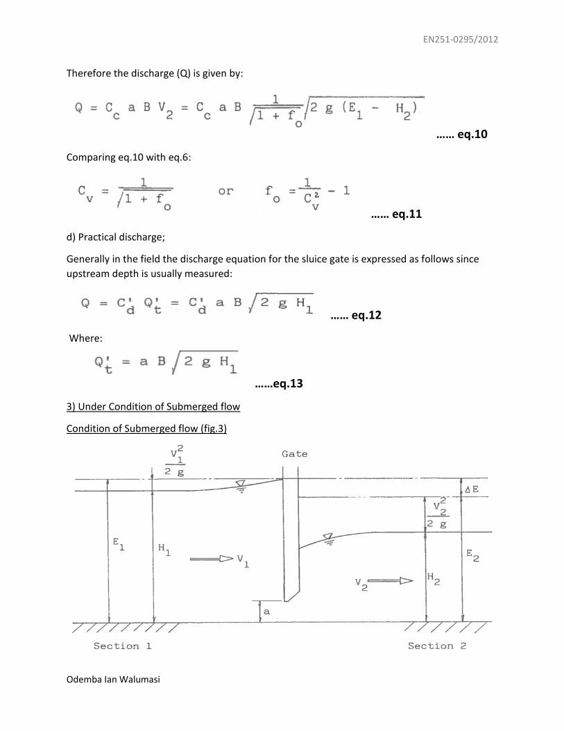
3) Under Condition of Submerged flow
Condition of Submerged flow (fig.3)

EN251-0295/2012
Odemba Ian Walumasi
a) Discharge equation;
The discharge through the sluice gate under the condition of submerged flow (fig.3) is given by
……eq.14
…… eq.15
And
…… eq.16
eq.14 is the same as that of a submerged orifice.
b) Experiments by Henry;
H.R. Henry suggested the following equation to find discharge through a sluice gate and the
coefficient of discharge (C’d) H1/a values and H2/a values as shown in fig.4:
……eq.17
…… eq.18
H.R. Henry’s equation graphical illustration (fig.4)

EN251-0295/2012
Odemba Ian Walumasi
Objectives of the experiment
To determine coefficient of discharge for the sluice gate
To understand the difference in coefficient f discharge for condition of free outflow and
submerged outflow.
MATERIALS AND METHODS
Apparatus (Materials)
1. An adjustable-slope rectangular open channel with point gauges.
2. An adjustable height suppressed weir
3. A steady water supply system
4. A V-notch with hook gauge
5. A sluice gate with rubber packings
6. A steel tape measure
7. A thermometer
Set up of experiment apparatus (fig.5)

EN251-0295/2012
Odemba Ian Walumasi
Procedure (Method)
1) The width of channel and temperature of water was measured.
2) The channel was set horizontal.
3) The opening height of the sluice gate was set between 2.5cm and 3.0cm and measured
accurately using the tape measure.
4) The crest level of the V-notch was recorded with the hook gauge.
5) The channel bed levels upstream (section 1) and downstream (section 2) of the sluice
gate were measured with a point gauge.
6) The steady water supply system operation was started and discharge set to be small.
7) After the flow became steady (free outflow) the depths at section 1 and section 2 were
measured.
8) Head above the V-notch was measured.
9) The state of flow through the sluice gate was observed, and contraction of flow
confirmed.
10) Discharge was increased so that another free flow can be observed repeating steps (7),
(8) and (9). The discharge at section 1 should not be too large.
11) The discharge was set small again, and the gate opening height set between 3.0cm and
4.0cm then adjusted such that a suppressed submerged outflow occurred.
12) Step (8) was executed, and steps (7) and (9) repeated at least five times, changing the
downstream depth using suppressed weir.
13) Discharge was increased such that a submerged outflow is observed, and step (12)
repeated.
RESULTS
The following requirements were met for presentation of results;
1) Condition of Free outflow
1) Preparing an arrangement table (table 2) and filling in the columns with data.
2) Calculating the following values and filling in the table;
a) Discharge (Qa)
b) Velocity of flow at section 1 (V1)
c) Velocity of flow at section 2 (V2)
d) Specific energy at each section (E1)
e) Coefficient of contraction (Cc)
f) Theoretical discharge (Qt)

EN251-0295/2012
Odemba Ian Walumasi
g) Coefficient of discharge (Cd)
h) Coefficient of velocity (Cv)
i) Coefficient of loss due to outflow (fo)
j) Theoretical discharge obtained from the depth at section 1(eq.13)(Q’t)
k) Coefficient of discharge produced by eq.12 (C’d)
3) Plotting values of H1/a on abscissa and coefficient of discharge (Cd) on ordinate on section
graph.
4) Plotting the depth at section 1 (H1) on abscissa and discharge (Q) on ordinate on log-log
graph. Draw the equation Q’t = aB√ (2g.H1).
5) Plotting H1/a on abscissa and coefficient of loss due to outflow (fo) on ordinate on section
graph.
6) Plotting H1/a on abscissa and coefficient of contraction (Cc) on ordinate on section graph.
2) Condition of submerged outflow
1) Preparing an arrangement table (table 5) and filling in the columns with data.
2) Calculating the following values and filling in the table;
a) Discharge (Qa)
b) Velocity of flow at section 1 (V1)
c) Specific energy at each section (E1)
d) Ratio of depth at section 1 to depth at section 2 (H1/H2)
e) Ratio of depth at section 1 to the opening height of gate (H1/a)
f) Ratio of depth at section 2 to the opening height of gate (H2/a)
g) Theoretical discharge (Qt)
h) Coefficient of discharge (Cd)
i) Theoretical discharge obtained from depth at section 1 (eq.18) (Q’t)
j) Coefficient of discharge produced by eq.12 (C’d)
3) Plot value of H1/H2 on abscissa and coefficient of discharge on ordinate.
4) Plot value of H1/a on abscissa and coefficient of discharge (Cd) and coefficient of discharge
(C’d) introduced in eq.17 on ordinate on section graph.

EN251-0295/2012
Odemba Ian Walumasi
Data Sheet (Free outflow conditions)
Fundamental data I (table 1)
Properties of water Temperature 24 °C
Density (ρ) 1000 Kg/m3
Dimensions of channel Width (B) 0.30 m
Channel bed
level
Section1 0.478 m
Section2 0.477 m
Properties of V-notch Half angle of V-notch (Ѳ) 45 °
Coefficient of discharge (Cdv) 0.65
Coefficient (KV) 1.5355
Crest level 0.2150 m
Dimensions of sluice gate Width (B) 0.30 m
Opening height (a) 0.026 m
Operation data I (table 2)
stag
e
v-notch point gauge depth
velo
city
at
sect
ion
1
(V1)
(m/s
)
velo
city
hea
d
(V1
2/2
g) (
m)
spec
ific
en
ergy
(E 1
)
(m)
Fro
ud
e's
nu
mb
er a
t
sect
ion
1 (
Fr1)
Fro
ud
e's
nu
mb
er a
t
sect
ion
2 (
Fr2)
read
ing
(m)
hea
d (
HV)
(m)
dis
char
ge (
Q)
(*1
0-3
m3/s
)
sect
ion
1 (
m)
sect
ion
2 (
m)
sect
ion
1 (
H1)
(m)
sect
ion
2 (
H2)
(m)
1 0.115
0.1 4.856
0.552
0.493
0.074
0.016
0.2187
0.0024
0.0764
0.066
6.52
2 0.109
0.106
5.617
0.599
0.494
0.121
0.017
0.1547
0.0012
0.1222
0.02 7.27
3 0.107
0.108
5.886
0.567
0.494
0.089
0.017
0.2204
0.0025
0.0915
0.055
7.99
4 0.104
0.111
6.303
0.577
0.494
0.099
0.017
0.2122
0.0023
0.1013
0.046
9.16
5 0.101
0.114
6.738
0.588
0.494
0.11 0.017
0.2042
0.0021
0.1121
0.039
10.46
6 0.099
0.116
7.037
0.608
0.494
0.13 0.017
0.1804
0.0017
0.1317
0.026
11.42

EN251-0295/2012
Odemba Ian Walumasi
Calculation I (table 3) St
age
dis
char
ge (
Q)
(*1
0-3
m3 /s
)
H1/a
coe
ffic
ien
t o
f co
ntr
acti
on
(Cc
= H
2/a
)
Theo
reti
cal d
isch
arge
(Q
t)
(*1
0-3
m3/s
)
coe
ffic
ien
t o
f d
isch
arge
(C
d)
coe
ffic
ien
t o
f ve
loci
ty (
Cv)
coe
ffic
ien
t o
f lo
ss d
ue
to
ou
tflo
w (
f o)
Theo
reti
cal d
isch
arge
fro
m
equ
atio
n (
Q' t)
(*1
0-3
m3/
s)
coe
ffic
ien
t o
f d
isch
arge
(C
' d)
1 4.856 2.846 0.6154 8.49 0.572 0.9295 0.1574 9.4 0.5166
2 5.617 4.654 0.6538 11.21 0.5011 0.7664 0.7025 12.02 0.4673
3 5.886 3.423 0.6538 9.43 0.6243 0.9549 0.0967 10.31 0.5709
4 6.303 3.808 0.6538 10.03 0.628 0.9605 0.0839 10.87 0.5799
5 6.738 4.231 0.6538 10.65 0.6327 0.9677 0.0679 11.46 0.588
6 7.037 5 0.6538 11.7 0.6015 0.9254 0.1677 12.46 0.5648
Data sheet II (Submerged outflow conditions)
Fundamental data II (table 4)
Dimensions of sluice gate Width (B) 0.30 m
Opening height (a) 0.034m
Properties of V-notch Coefficient (KV) 1.5355
Crest level 0.2150 m
Channel bed level Section1 0.478 m
Section2 0.477 m

EN251-0295/2012
Odemba Ian Walumasi
Operation data II (table 5)
stage
v-notch point gauge depth
velo
city
at
sect
ion
1
(V1)
(m)
velo
city
hea
d a
t se
ctio
n
1 (
V1
2/2
g) (
m)
spec
ific
en
ergy
(E 1
) (m
)
Rea
din
g (m
)
hea
d (
H)
(m)
dis
char
ge (
Q)
(*1
0-3
m3/s
)
sect
ion
1 (
m)
sect
ion
2 (
m)
sect
ion
1 (
H1)
(m)
sect
ion
2 (
H2)
(m)
1 A 0.117 0.098 4.617 0.58 0.542 0.102 0.065 0.1509 0.0012 0.1032
B 0.567 0.534 0.089 0.057 0.1729 0.0015 0.0905
C 0.533 0.53 0.055 0.053 0.2798 0.004 0.059
D 0.549 0.529 0.071 0.052 0.2168 0.0024 0.0734
E 0.546 0.528 0.068 0.051 0.2263 0.0026 0.0706
2 A 0.102 0.113 6.591 0.634 0.558 0.156 0.081 0.1408 0.001 0.157
B 0.63 0.547 0.152 0.07 0.1445 0.0011 0.1531
C 0.623 0.543 0.145 0.066 0.1515 0.0012 0.1462
D 0.605 0.535 0.127 0.058 0.173 0.0015 0.1285
E 0.591 0.535 0.113 0.058 0.1944 0.0019 0.1149
Calculation II (table 6)
stage
dis
char
ge (
Q)
(*1
0-3
m3/s
)
H1/H2
H1/a
H2/a
Theo
reti
cal d
isch
arge
(Q
t)
(*1
0-3
m3/s
)
coe
ffic
ien
t o
f d
isch
arge
(Cd)
Henry's Experiment
Theo
reti
cal d
isch
arge
fro
m e
qu
atio
n
(Q' t)
(*1
0-3
m3/s
)
coe
ffic
ien
t o
f
dis
char
ge (
C' d
)
1 A 4.617 0.637 3 1.91 8.83 0.5229 14.43 0.32
B 0.64 2.62 1.6 8.27 0.5583 13.48 0.3425
C 0.964 1.61 1.56 3.5 1.319 10.6 0.4356
D 0.732 2.08 1.53 6.61 0.6985 12.04 0.3835
E 0.75 2 1.5 6.32 0.7305 11.78 0.3919
2 A 6.591 0.519 4.59 2.38 12.46 0.529 17.84 0.3694
B 0.461 4.47 2.06 13.02 0.5062 17.61 3743
C 0.455 4.26 1.94 12.7 0.519 17.2 0.3832
D 0.457 3.73 1.71 11.87 0.5553 16.1 0.4094
E 0.513 3.32 1.71 10.6 0.6218 15.19 0.4339 The following graphs were drawn

EN251-0295/2012
Odemba Ian Walumasi
Graph 1: Q against H1/a; free outflow
Graph 2: Log Q against Log H1; free outflow
0
1
2
3
4
5
6
7
8
9
0 1 2 3 4 5 6 7 8
Dis
char
ge(Q
) (*
10
-3m
3/s
)
H1/a
Discharge(Q) against H1/a
Discharge(Q) against H1/aLinear (Discharge(Q) against H1/a)
0.6
0.8
Log
Q(D
isch
arge
)
Log H1
Log Q against Log H1
Log Qa against Log H1 Log Q' t against Log H1

EN251-0295/2012
Odemba Ian Walumasi
Graph 3: Fo against H1/a; free outflow
Graph 4: Cc against H1/a; free outflow
0
0.1
0.2
0.3
0.4
0.5
0.6
0.7
0.8
1.5 2 2.5 3 3.5 4 4.5 5 5.5
F o
H1/a
Fo against H1/a
Fo against H1/a
0.61
0.615
0.62
0.625
0.63
0.635
0.64
0.645
0.65
0.655
0.66
0 1 2 3 4 5 6
Cc
H1/a
Cc against H1/a
Cc against H1/a

EN251-0295/2012
Odemba Ian Walumasi
Graph 5: Cd against H1/H2; submerged outflow
Graph 5: Cd and C’d against H1/a; submerged outflow
0
0.2
0.4
0.6
0.8
1
1.2
1.4
0 0.2 0.4 0.6 0.8 1 1.2 1.4
Cd
H1/H2
Cd against H1/H2
Cd against H1/H2 Log. (Cd against H1/H2)
0
0.2
0.4
0.6
0.8
1
1.2
1.4
0 0.5 1 1.5 2 2.5 3 3.5 4 4.5 5
dis
char
ge c
oef
fici
ent
H1/a
Discharge coefficient against H1/a
Cd against H1/a C' d against H1/a

EN251-0295/2012
Odemba Ian Walumasi
DISCUSSION
The following consideration were made for discussion
1) Deriving eq.12 for discharge;
Bernoulli’s Equation is energy equation for an ideal fluid (friction and energy losses assumed negligible.) which is derived to the question for using to calculation in this laboratory as follow:
𝐙𝟏+ 𝐕𝟐
𝟐𝐠+ 𝐏
𝛄 = 𝐙𝟐+ 𝐕
𝟐
𝟐𝐠+ 𝐏
𝛄 …… eq.19
Velocity→ discharge, Q, Q=AV
𝐙𝟏 +(𝐐𝟏𝐀𝟏
)𝟐
𝟐𝐠 = 𝐙𝟐 +
(𝐐𝟐𝐀𝟐
)𝟐
𝟐𝐠 (1)
𝒚𝟏 +(𝑸𝟏𝑨𝟏
)𝟐
𝟐𝒈 = 𝒚𝟐 +
(𝑸𝟐𝑨𝟐
)𝟐
𝟐𝒈 (2)
Unit discharge, 𝑞 = 𝑄
𝐵
From (1);
𝐪𝟐
𝟐𝐠𝐲𝟏𝟐 − 𝐪𝟐
𝟐𝐠𝐲𝟐𝟐 = 𝒚𝟐 − 𝒚𝟏 (3)
(𝒒𝟐
𝟐𝒈) ( 𝟏
𝒚𝟏𝟐 −
𝟏
𝒚𝟐𝟐) = 𝒚𝟐 − 𝒚𝟏 (4)
(𝒒𝟐
𝟐𝒈) (𝒚𝟐
𝟐−𝒚𝟏𝟐
𝒚𝟏𝟐𝒚𝟐
𝟐 ) = 𝒚𝟐 − 𝒚𝟏 (5)
(𝒒𝟐
𝟐𝒈) ((𝒚𝟐+𝒚𝟏)(𝒚𝟐−𝒚𝟏)
𝒚𝟏𝟐𝒚𝟐
𝟏 ) = 𝒚𝟐 − 𝒚𝟏 (6)
𝒒𝟐 = (𝒚𝟏
𝟐𝒚𝟐𝟐)×(𝒚𝟐−𝒚𝟐)×𝟐𝒈
(𝒚𝟐+𝒚𝟏)(𝒚𝟐−𝒚𝟏) (7)
𝒒𝟐 = (𝒚𝟏
𝟐𝒚𝟐𝟐×𝟐𝒈)
(𝒚𝟐+𝒚𝟏) (8)
Q = √𝒚𝟏
𝟐𝒚𝟐𝟐×𝟐𝒈
𝒚𝟐+𝒚𝟏 (9)
Q = 𝒚𝟏𝒚𝟐√𝟐𝒈
𝒚𝟐+𝒚𝟏 (10)
Q = 𝑪𝒅𝑾√𝟐𝒈𝒚𝟏 (11)
Cd = Coefficient of discharge

EN251-0295/2012
Odemba Ian Walumasi
𝐪(𝐚𝐜𝐭𝐮𝐚𝐥)
𝐪(𝐭𝐡𝐞𝐨𝐫𝐲) = Cd< 1 (12)
𝑪𝒅 = 𝒒
𝑾√𝟐𝒈𝒚𝟏
Bernoulli’s Equation:
𝒚𝟏 + 𝑽𝟐
𝟐𝒈 = 𝒚𝟐 + 𝑽𝟐
𝟐𝒈 (13)
𝒚𝟏 + 𝒒𝟐
𝟐𝒈𝒚𝟏 = 𝒚𝟐 + 𝒒𝟐
𝟐𝒈𝒚𝟏 (14)
Momentum Equation: F = ma (15)
𝒚𝟐𝟐
𝟐+ 𝒒𝟐
𝒈𝒚𝟐 = 𝒚𝟑
𝟐
𝟐+ 𝒒𝟐
𝒈𝒚𝟑 (16)
Free Flow
Q = 𝑪′𝒅𝑾√𝟐𝒈𝒚𝟏 …… eq.20
Submerged Flow
q = 𝑪𝒅𝑾√𝟐𝒈𝒚𝟏 …… eq.21
Compare eq.20 with eq.12
2) Stating the facts:
The graphs of coefficients of discharge against H1/a (graph 5) for submerged outflow and graph
2 as a predictor for free outflow followed the expected trend laid by H.R. henry equations used
in the analysis (fig.4)
3) Finding Froude’s number at each section for free outflow: (table 2)
CONCLUSION
Objectives of experiment were met Cdm = 0.564 for submerged outflow and Cdm = 0.612 for free
outflow.
CITED WORK
Lecture notes
Manual for Hydraulics and Water resources JKUAT, School of Civil Construction
and Environmental Engineering
Gate Lip Hydraulics under Sluice Gate, Department of Dam and Water Resources,
College of Electronic Engineering, University of Mosul, Mosul, Iran


