Embed Size (px)
Citation preview

Ch 4. Shear Flow Dispersion
4-1
Chapter 4 Shear Flow Dispersion
Contents
4.1 Dispersion in laminar Shear Flow
4.2 Dispersion in Turbulent Shear Flow
4.3 Dispersion in Unsteady Shear Flow
4.4 Dispersion in Two Dimensions
Objectives:
1) Derive shear flow dispersion equation using Taylor’ analysis (1953, 1954)
- laminar flow in pipe
- turbulent flow
→ apply Fickian model to dispersion
→ reasonably accurate estimate of the rate of longitudinal dispersion in rivers
and estuaries
2) Extend dispersion analysis to unsteady flow and two-dimensional flow
Taylor, Geoffrey – English fluid mechanician

Ch 4. Shear Flow Dispersion
4-2
4.1 Dispersion in Laminar Shear Flow
4.1.1 Introductory Remarks
∙ Taylor's analysis (1953) in laminar flow in pipe
Consider laminar flow in pipe with velocity profile shown below.
Assume two molecules are being carried in the flow; one in the center and one near the wall.
1) Rate of separation caused by the difference in advective velocity ≫ separation by molecular motion
2) Because of molecular diffusion, each molecule moves at random walk back
and forth across the cross section
3) Fickian diffusion equation can describe the
.
→ motion of single molecule is the sum of a series of independent steps of
random length.
spread of particles along the axis
of the pipes, except that since the step length and time increment are much
different from those of molecular diffusion. We expect to find a different value
of diffusion coefficient.
0u
a
Ch 4. Shear Flow Dispersion
4-3
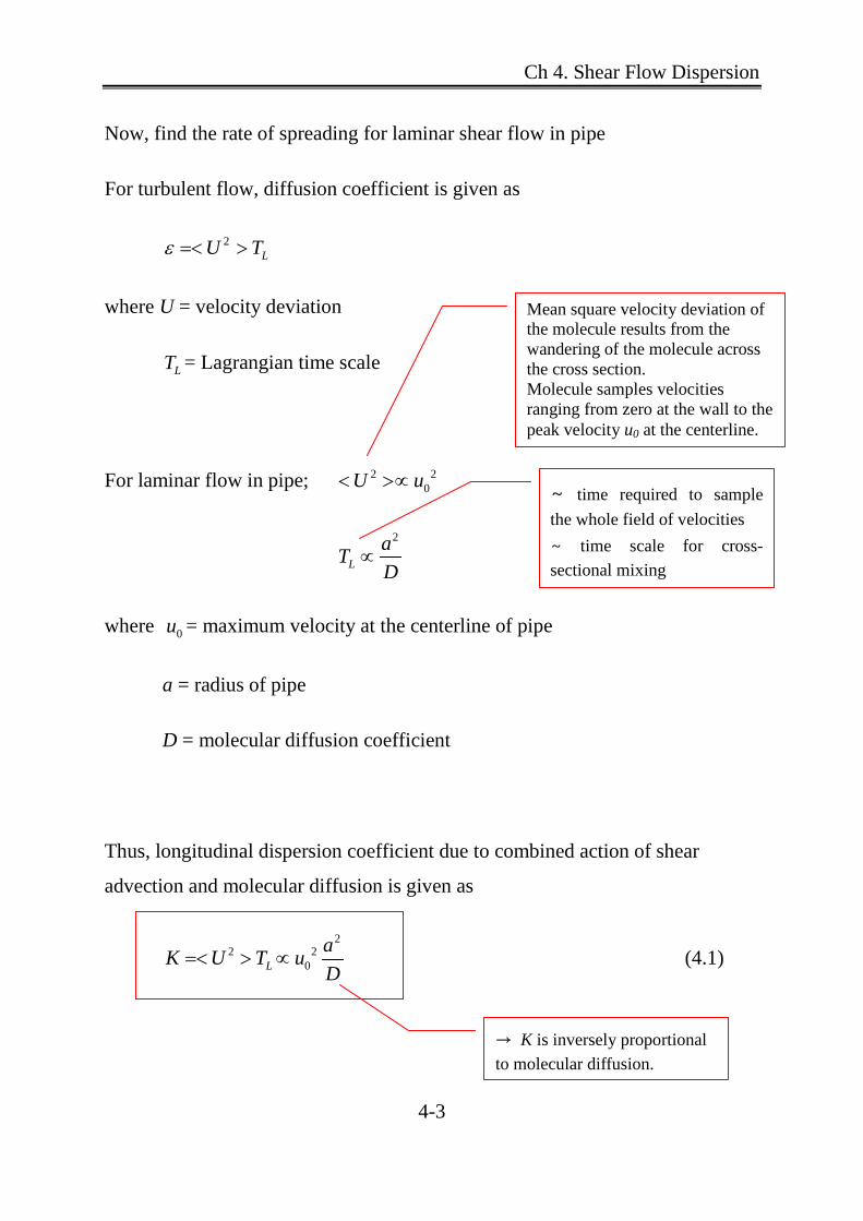
Now, find the rate of spreading for laminar shear flow in pipe
For turbulent flow, diffusion coefficient is given as
2LU Tε =< >
where U = velocity deviation
LT = Lagrangian time scale
For laminar flow in pipe; 2 20U u< >∝
2
LaTD
∝
where 0u = maximum velocity at the centerline of pipe
a = radius of pipe
D = molecular diffusion coefficient
Thus, longitudinal dispersion coefficient due to combined action of shear
advection and molecular diffusion is given as
22 2
0LaK U T uD
=< > ∝ (4.1)
∼ time required to sample the whole field of velocities ∼ time scale for cross-sectional mixing
Mean square velocity deviation of the molecule results from the wandering of the molecule across the cross section. Molecule samples velocities ranging from zero at the wall to the peak velocity u0 at the centerline.
→ K is inversely proportional to molecular diffusion.

Ch 4. Shear Flow Dispersion
4-4
4.1.2 A Generalized Introduction
(a) example velocity distribution (b) transformed coordinate system
moving at the mean velocity
Consider the 2-D laminar flow with velocity variation u(y) between walls
Define the cross-sectional mean velocity as
0
1 hu udy
h= ∫ (4.2)
Then, velocity deviation is
( )'u u y u= − (4.3)
Let flow carry a solute with concentration C(x, y) and molecular diffusion
coefficient D.
Define the mean concentration at any cross section as
( )0
1 , ( )h
C Cdy C f x f yh
= = ≠∫ (4.4)
Then, concentration deviation is

Ch 4. Shear Flow Dispersion
4-5
( )' ' ', ( , )C C y C C C x y= − = (4.4a)
Now, use 2-D diffusion equation with
2 2
2 2
C C C C Cu v D Dt x y x y
∂ ∂ ∂ ∂ ∂+ + = +
∂ ∂ ∂ ∂ ∂
only flow in x-direction (v =0)
(1)
Substitute (4.2)~(4.4) into (1)
( )2 2
' ' ' ' '2 2( ) ( ) ( ) ( )C C u u C C D C C C C
t x x y ∂ ∂ ∂ ∂
+ + + + = + + + ∂ ∂ ∂ ∂ (4.5)
Now, simplify (4.5) by a transformation of coordinate system whose origin
moves at the mean flow velocity
1x ut ux tξ ξξ ∂ ∂
= − → = = −∂ ∂
0 1tx tτ ττ ∂ ∂
= → = =∂ ∂
Chain rule
x x xξ τ
ξ τ ξ∂ ∂ ∂ ∂ ∂ ∂= + =
∂ ∂ ∂ ∂ ∂ ∂ (b)
ut t t
ξ τξ τ ξ τ
∂ ∂ ∂ ∂ ∂ ∂ ∂= + = − +
∂ ∂ ∂ ∂ ∂ ∂ ∂ (c)
Substitute Eq. (b)-(c) into Eq. (4.5)
0Cy
∂=
∂

Ch 4. Shear Flow Dispersion
4-6
( )2 2 '
' ' ' ' '2 2( ) ( ) ( ) ( ) Cu C C C C u u C C D C C
yξ τ ξ ξ ∂ ∂ ∂ ∂ ∂
− + + + + + + = + + ∂ ∂ ∂ ∂ ∂
2 2 '' ' ' '
2 2( ) ( ) ( ) CC C u C C D C Cyτ ξ ξ
∂ ∂ ∂ ∂+ + + = + + ∂ ∂ ∂ ∂
(4.8)
→ view the flow as an observer moving at the mean velocity
→ 'u is only observable velocity
Now, neglect longitudinal diffusion because rate of spreading along the flow
direction due to velocity difference greatly exceed that due to molecular
diffusion
2' ' '
2( ) ( )u C C D C Cξ ξ∂ ∂
+ +∂ ∂
.
' ' 2 '' '
2
C C C C Cu u Dyτ τ ξ ξ
∂ ∂ ∂ ∂ ∂+ + + =
∂ ∂ ∂ ∂ ∂ (4.9)
→ This equation is still intractable because 'u varies with y.
→ General solution cannot be found because a general procedure for dealing
with differential equations with variable coefficients is not available.
Now introduce Taylor's assumption
→ discard three terms to leave the easily solvable equation for
' ( )C y
2 ''
2
C Cu Dyξ
∂ ∂=
∂ ∂ (4.10)

Ch 4. Shear Flow Dispersion
4-7
[Re] Derivation of Eq. (4.10) using order of magnitude analysis
Take average over the cross section of Eq. (4.9)
→ apply the operator 0
1 ( )h
dyh ∫
' ' 2 '' '
2
C C C C Cu u Dyτ τ ξ ξ
∂ ∂ ∂ ∂ ∂+ + + =
∂ ∂ ∂ ∂ ∂
Apply Reynolds rule of average '
' 0C Cuτ ξ
∂ ∂+ =
∂ ∂ (4.11)
Subtract Eq.(4.11) from Eq.(4.9)
' ' ' 2 '
' ' '2
C C C C Cu u u Dyτ ξ ξ ξ
∂ ∂ ∂ ∂ ∂+ + − =
∂ ∂ ∂ ∂ ∂
Assume ',C C are well behaved, slowly varying functions and 'C C>>
Then ' '
' ' ',C C Cu u uξ ξ ξ∂ ∂ ∂
>>∂ ∂ ∂
Thus we can drop ' '
' ',C Cu uξ ξ
∂ ∂∂ ∂
' 2 ''
2
C C CD uyτ ξ
∂ ∂ ∂= −
∂ ∂ ∂ (d)
' Cuξ∂
−∂
= source term of variable strength
→ Net addition by source term is zero because the average of 'u is zero.

Ch 4. Shear Flow Dispersion
4-8
Assume that Cξ∂∂
remains constant for a long time, so that the source is constant.
Then, Eq. (a) can be assumed as '
0Cτ
∂=
∂
steady state.
→
Then (a) becomes 2 '
'2
C Cu Dyξ
∂ ∂=
∂ ∂
(A) (B)
→ same as Eq. (4.10)
→ cross sectional concentration profile '( )C y is established by a balance
between longitudinal advective transport and cross sectional diffusive transport.
<Fig. 4.3> The balance of advective flux versus diffusive flux
In balance, net transport = 0
longitudinal advective transport
cross sectional diffusive transport
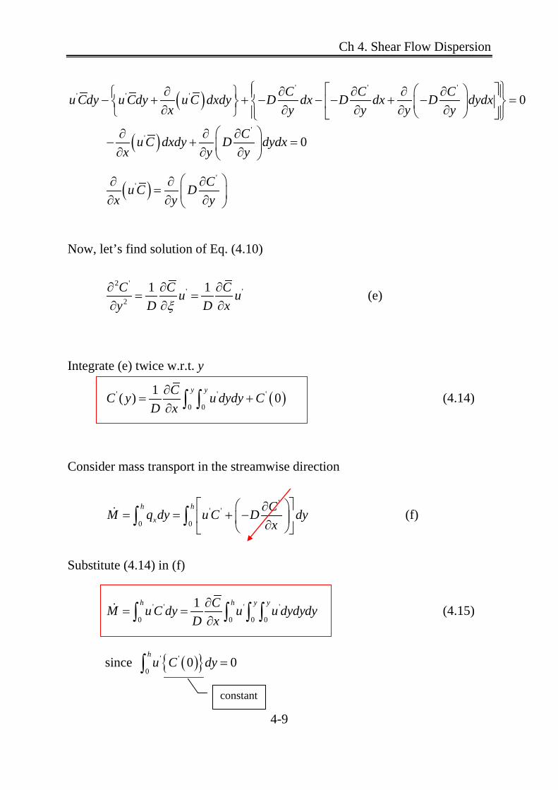
Ch 4. Shear Flow Dispersion
4-9
( )' ' '
' ' ' 0C C Cu Cdy u Cdy u C dxdy D dx D dx D dydxx y y y y
∂ ∂ ∂ ∂ ∂ − + + − − − + − = ∂ ∂ ∂ ∂ ∂
( )'
' 0Cu C dxdy D dydxx y y
∂ ∂ ∂− + = ∂ ∂ ∂
( )'
' Cu C Dx y y
∂ ∂ ∂= ∂ ∂ ∂
Now, let’s find solution of Eq. (4.10)
2 '
' '2
1 1C C Cu uy D D xξ
∂ ∂ ∂= =
∂ ∂ ∂ (e)
Integrate (e) twice w.r.t. y
( )' ' '
0 0
1( ) 0y yCC y u dydy C
D x∂
= +∂ ∫ ∫ (4.14)
Consider mass transport in the streamwise direction
'
' '
0 0
h h
xCM q dy u C D dyx
∂= = + − ∂ ∫ ∫ (f)
Substitute (4.14) in (f)
' ' ' '
0 0 0 0
1h h y yCM u C dy u u dydydyD x∂
= =∂∫ ∫ ∫ ∫ (4.15)
since ( ){ }' '
00 0
hu C dy =∫
constant

Ch 4. Shear Flow Dispersion
4-10
→ Eq. (4.15) means that total mass transport in the streamwise direction is
proportional to the concentration gradient
CMx
∂∝∂
in that direction.
(g)
→This is exactly the same result that we found for molecular diffusion.
Cq Dx
∂= −
∂
But this is
q
diffusion due to whole field of flow.
Let = rate of mass transport per unit area
1M Cq K
h x∂
= = −× ∂
per unit time
Then, (g) becomes
(h)
where h = depth = area per unit width of flow
K = longitudinal dispersion coefficient (= bulk transport coefficient)
→ express as the diffusive property of the velocity distribution (shear flow)
Then, (h) becomes
CM hKx
∂= −
∂ (4.16)
Comparing Eq. (4.15) and Eq. (4.16) we see that
' '
0 0 0
1 h y yK u u dydydy
hD= − ∫ ∫ ∫ (4.17)
Ch 4. Shear Flow Dispersion
4-11
1KD
∝
Now, we can express this transport process due to velocity distribution as a one-
dimensional Fickian-type diffusion equation in moving coordinate system.
2
2
C CKτ ξ
∂ ∂=
∂ ∂ (4.18)
Return to fixed coordinate system 2
2
C C Cu Kt x x
∂ ∂ ∂+ =
∂ ∂ ∂ (4.19)
→ 1-D advection-dispersion equation
C , u = cross-sectional average values
▪ Balance of advection and diffusion in Eq. (4.10)
Suppose that at some initial time t = 0 a line source of tracer is deposited in the
flow (Fig. 4.4a).
→ Initially the line source is advected and distorted by the velocity profile.
At the same time the distorted source begins to diffuse across the cross section.
→ Shortly we see a smeared cloud with trailing stringers along the boundaries
(Fig. 4.4b).
During this period, advection and diffusion are by no means in balance.

Ch 4. Shear Flow Dispersion
4-12
→ Taylor’s assumption does not apply.
→ Cross-sectional average concentration is skewed distribution (Fig. 4.4c).
If we wait much longer time, the cloud of tracer extends over a long distance
C
in
the x direction.
→ varies slowly along the channel, and Cx
∂∂
is essentially constant over a
long period of time.
→ 'C becomes small because cross-sectional diffusion
2
0.4 htD
<
evens out cross-
sectional concentration gradient.
Chatwin (1970) suggested
i) Initial period:
→ advection > diffusion
ii) Taylor period: 2
0.4 htD
>
→ advection ≈ diffusion
→ can use Eq. (4.19)
→ The initial skew degenerates into the normal distribution. 2
2Ktσ∂
=∂

Ch 4. Shear Flow Dispersion
4-13
4.1.3 A Simple Example
Consider laminar flow between two plates → Couette flow
Fig. 4.5 Velocity profile and the resulting concentration profile
( ) yu y Uh
=
2
2
1 0h
hyu U dy
h h−= =∫
'u u∴ =
Suppose 2ht
D> → tracer is well distributed
→ Taylor’s analysis can be applied
From Eq. (4.14)
( )' ' '
0 0
1 (0)y yCC y u dydy C
D x∂
= +∂ ∫ ∫
'
2 2
1 ( )2
y yh h
C Uy hdydy CD x h− −
∂= + −
∂ ∫ ∫ (a)
0.042
Ch 4. Shear Flow Dispersion
4-14
2 '
22
1 ( )2 2
yyh
h
C U hy dy CD x h−
−
∂ = + − ∂ ∫
2'
2
1 ( )2 8 2
yh
C Uy Uh hdy CD x h−
∂= − + − ∂
∫
3'
2
1 ( )6 8 2
y
h
C Uy Uh hy CD x h
−
∂= − + − ∂
3 2 2'1 ( )
6 8 48 16 2C Uy Uh Uh Uh hy C
D x h ∂
= − + − + − ∂
3 2 3'1
2 3 4 12 2C U y h h hy C
D x h ∂ = − − + − ∂
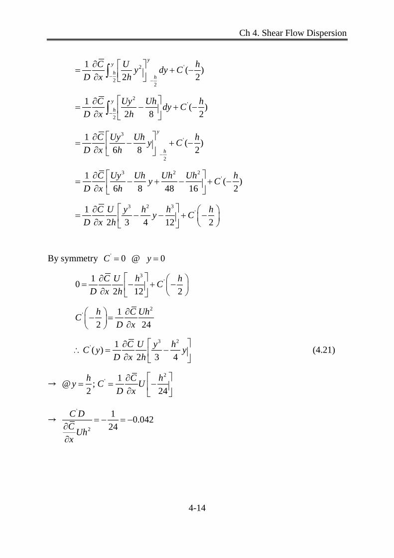
By symmetry ' 0 @ 0C y= =
3'10
2 12 2C U h hC
D x h ∂ = − + − ∂
2' 1
2 24h C UhC
D x∂ − = ∂
3 2' 1( )
2 3 4C U y hC y y
D x h ∂
∴ = − ∂ (4.21)
→ 2
' 1@ ;2 24h C hy C U
D x ∂
= = − ∂
→ '
2
1 0.04224
C DC Uhx
= − = −∂∂
Ch 4. Shear Flow Dispersion
4-15
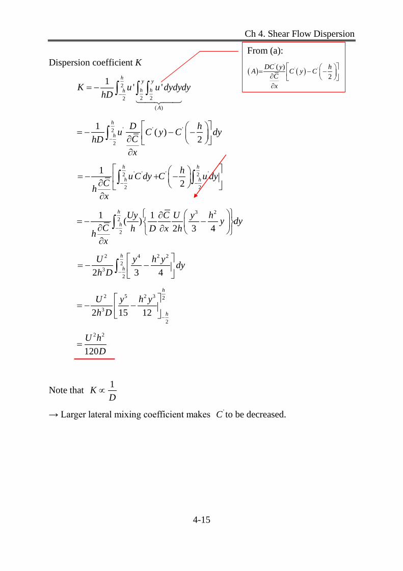
Dispersion coefficient K
2
2 22
( )
1 ' 'h y y
h hh
A
K u u dydydyhD −
= − ∫ ∫ ∫
' ' '2
2
1 ( )2
h
hD hu C y C dyChDx
−
= − − − ∂ ∂
∫
' ' ' '2 2
2 2
12
h h
h hhu C dy C u dy
Chx
− −
= − + − ∂ ∂
∫ ∫
3 22
2
1 1( )2 3 4
h
hUy C U y h y dy
C h D x hhx
−
∂= − − ∂ ∂
∂
∫
2 4 2 22
322 3 4
h
hU y h y dyh D −
= − −
∫
2 5 2 3 2
3
22 15 12
h
h
U y h yh D
−
= − −
2 2
120U h
D=
Note that 1KD
∝
→ Larger lateral mixing coefficient makes 'C to be decreased.
From (a):
( ) ( )'
' '( )2
DC y hA C y CCx
= − − ∂ ∂

Ch 4. Shear Flow Dispersion
4-16
4.1.4 Taylor's Analysis of Laminar Flow in a Tube
Consider axial symmetrical flow in a tube → Poiseuille flow
Tracer is well distributed over the cross section.
( )2
0 21 ru r ua
= −
→ paraboloid (a)
Integrate u to obtain mean velocity
2dQ u rdrπ≅
2
0 202 1
a rQ r u dra
π ∴ = −
∫

Ch 4. Shear Flow Dispersion
4-17
212
0 202 1r r ru a d
a a aπ
= −
∫12 2
0 02 (1 )u a z z dzπ= −∫
12 2
20
0
22 4z zu aπ
= −
2
02a uπ
=
By the way, 2Q u aπ= ⋅
0
2uu∴ =
2-D advection-dispersion equation in cylindrical coordinate is
2 2 2
0 2 2 2
11C r C C C Cu Dt a x r r r x
∂ ∂ ∂ ∂ ∂+ − = + + ∂ ∂ ∂ ∂ ∂
(b)
Shift to a coordinate system moving at velocity 0
2u
Neglect Ct
∂∂
and 2
2
Cx
∂∂
as before
Let , ,rz x ut taξ τ= = − =
Decompose C, then (b) becomes 2 2 ' '
202
1 1( )2
u a C C CzD z z zξ
∂ ∂ ∂− = +
∂ ∂ ∂
'
0Cz
∂=
∂ at 1z =
Integrate twice w.r.t. z

Ch 4. Shear Flow Dispersion
4-18
2' 2 40 1
8 2u a CC z z const
D x∂ = − + ∂
(c)
' '1
A
MK u C dAC CA Ax x
= − = −∂ ∂∂ ∂
∫
(d)
Substitute (a), (c) into (d), and then perform integration 2 2
0
192a uK
D=
[Example] Salt in water flowing in a tube 5 210 / secD cm−=
0 1 / secu cm=
2a mm=
( )6
(0.01) 0.00440 2000
1 10eudRv −= = = <<
× → laminar flow
( ) ( )( )
2 22 22 60
5
0.2 121 / sec 10
192 192 10a uK cm D
D −= = = ≈
☞ Initial period
( )( )
22
0 5
0.4 0.20.4 1600sec 27min
10atD −
= = = =
00 0 02
ux ut t= =
( )( )0.5 1600 800cm= =
800 40000.2
a= =
0x x> → 1-D dispersion model can be applied

Ch 4. Shear Flow Dispersion
4-19
Homework Assignment No. 4-1
Due: Two weeks from today
A hypothetical river is 30 m wide and consists of three "lanes", each 10m
in width. The two outside lanes move at 0.2 m/sec and the middle lane at
0.4m/sec. Every tm seconds complete mixing across the cross section of the river
(but not longitudinally) occurs. An instantaneous injection of a conservative
tracer results in a uniform of 100mg/ℓ in the water 2 m upstream and
downstream of the injection point. The concentration is initially zero elsewhere.
As the tracer is carried downstream and is mixed across the cross-section of the
stream, it also becomes mixed longitudinally, due to the velocity difference
between lanes
1) Mathematically simulate the tracer concentration profile
(concentration vs. longitudinal distance) as a function of time for
several (at least four) values of tm including 10 sec.
, even though there is no longitudinal diffusion within lanes. We
call this type of mixing "dispersion".

Ch 4. Shear Flow Dispersion
4-20
2) Compare the profiles and decide whether you think the effective
longitudinal mixing increases or decrease as tm increases.
This "scenario" represents the one-dimensional unsteady-state advection
and longitudinal dispersion of an instantaneous impulse of tracer for which the
concentration profile follow the Gaussian plume equation
( )2
44x UtMC exp
KtKtπ
− = −
in which x = distance downstream of the injection point, M = mass injected
width of the stream, K = longitudinal dispersion coefficient, U = bulk velocity
of the stream (flowrate/cross-sectional area), t = elapsed time since injection.
3) Using your best guess of a value for U, find a best-fit value for K for
each and for which you calculated a concentration profile. Tabulate of
plot the effective K as a function tm of and make a guess of what you
think the functional form is.

Ch 4. Shear Flow Dispersion
4-21
◆ Dispersion mechanism in a hypothetical river
1) 3 lanes of different velocities
2) Every tm seconds complete mixing occurs across the cross section of the river
(but not longitudinally) occurs, after shear advection is completed.
→ sequential mixing model
0xC
x xε∂ ∂ → ∂ ∂
2
my
Wtε
≅
3) Instantaneous injection
mt = 10 s; au =0.2 m/s; x∆ =2 m
W

Ch 4. Shear Flow Dispersion
4-22
t=tm +: After lateral mixing
0 67 100 33 0
0 67 100 33 0
0 67 100 33 0
(iii) t= 2 tm -: After shear advection t= 2 tm
+: After lateral mixing
0 0 67 100 33 0 0 0 45 89 55 11 0
0 0 0 67 100 33 0 0 45 89 55 11 0
0 0 67 100 33 0 0 0 45 89 55 11 0
ii) t=tm -

Ch 4. Shear Flow Dispersion
4-23

Ch 4. Shear Flow Dispersion
4-24
[Re] Longitudinal Dispersion in 2-lane river
α = Area fraction of river
occupied by slow lane
0 1α≤ ≤
Su u=
Fu u u= + ∆
u = cross-sectional mean velocity
( )( )1u u uα α= + − + ∆
Consider deviations:
( )( )( )
1
1S Su u u u u u u
u u u u u u u
α α
α α α α
′ = − = − − − + ∆
= − − − ∆ + + ∆ = − − ∆
( )( )1F Fu u u u u u u u u u uu
α αα
′ = − = + ∆ − = + ∆ − − − + ∆
= ∆
(i) Before any processes
mx u t∆ = ∆ ⋅
1 α−
α
u u+ ∆
u
Fast
Slow
1 α−
α
uC
uC
F
S
dC
dC
x∆ x∆
Ch 4. Shear Flow Dispersion
4-25
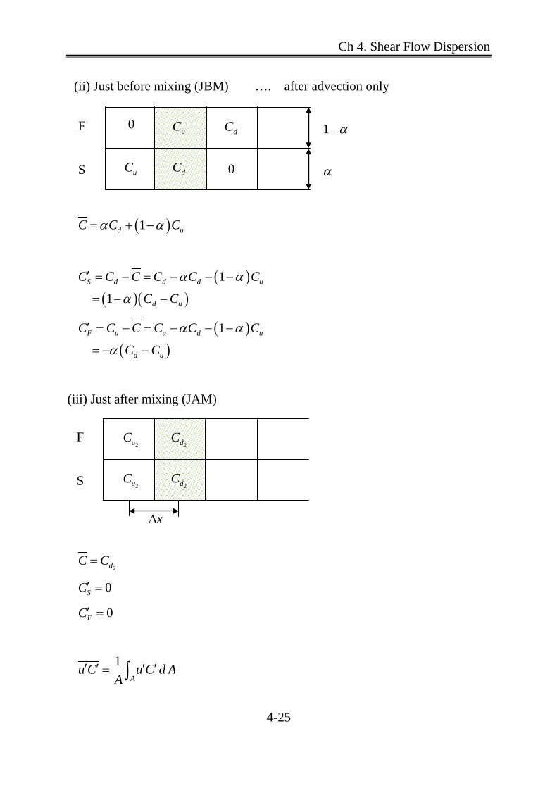
(ii) Just before mixing (JBM) …. after advection only
( )1d uC C Cα α= + −
( )( )( )
1
1S d d d u
d u
C C C C C C
C C
α α
α
′ = − = − − −
= − −
( )( )
1F u u d u
d u
C C C C C C
C C
α α
α
′ = − = − − −
= − −
(iii) Just after mixing (JAM)
2dC C=
0SC′ =
0FC′ =
1A
u C u C d AA
′ ′ ′ ′= ∫
1 α−
α
0
uC
F
S
uC
dC
dC
0
2uC
2uC
F
S
2dC
2dC
x∆

Ch 4. Shear Flow Dispersion
4-26
( ) ( ){ }( ) ( )( ){ }
( ) ( )( ){ ( )[ ] ( )( ) }
( ) ( )
JBM JAM
2
121 121 1 1 1212
S F
d u d u
d u
u C u C u C
u C u C
u C C u C C
u C C
α α
α α α α α α
α α
′ ′ ′ ′ ′ ′≅ +
′ ′ ′ ′= + −
= − − ∆ − − + − ∆ − −
= − ∆ −
d u
m
C C Cx ut
∂ −≈
∂ ∆
( ) ( )( )
( )( )
2
22
12
12
d u
d u
m
m
u C Cu CKC CC
utx
u t
α α
α α
− ∆ −′ ′= − =
−∂∆∂
= − ∆
<Example>
23
α = ; 0.2u∆ = ; 10 secmt =
( )2
21 2 2 0.2 0.00442 3 3 m mK t t = − =
5mt = 10 20 30
0.0222K = 0.0444 0.0889 0.1333

Ch 4. Shear Flow Dispersion
4-27
4.1.5 Aris's Analysis
Aris (1956) proposed the concentration moment method in which he obtain
Taylor’s main results without stipulating the feature of the concentration
distribution.
Begin with 2-D advective-diffusion equation in the moving coordinate system
to analyze the flow between two plates (Fig. 4.5)
2 2'
2 2
C C C Cu Dyτ ξ ξ
∂ ∂ ∂ ∂+ = + ∂ ∂ ∂ ∂
(4.29)
(1) (2) (3) (4)
Now, define the thp moments of the concentration distribution
( ) ( ),pPC y C y dξ ξ ξ
∞
−∞= ∫ (4.30)
Define cross-sectional average of thp moment
1 ( )p P PAM C C y dA
A= = ∫
Take the moment of Eq. (4.29) by applying the operator ( )P dξ ξ∞
−∞∫
(1) pp p CC d Cdξ ξ ξ ξτ τ τ
∞ ∞
−∞ −∞
∂∂ ∂= = =
∂ ∂ ∂∫ ∫ ← Leibnitz rule
[Re] Leibnitz formula
1 1
0 0
u u
u u
f ddx fdxdα α
∂=
∂∫ ∫
Ch 4. Shear Flow Dispersion
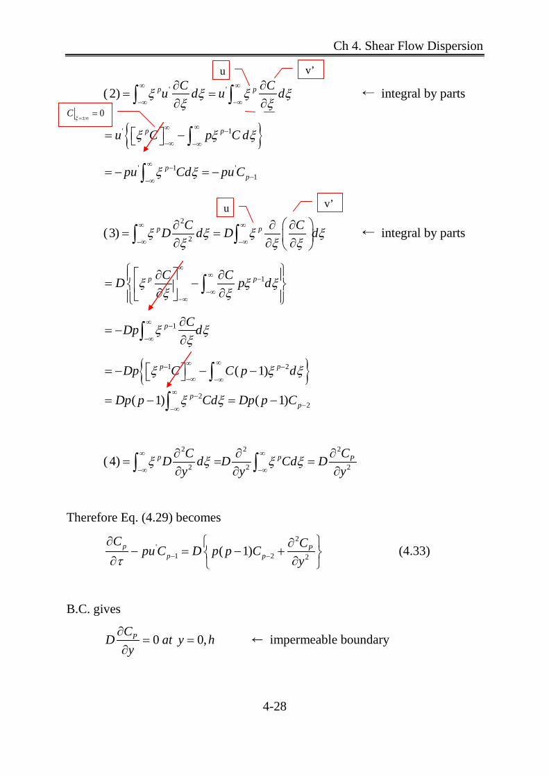
4-28
( ' '2) p pC Cu d u dξ ξ ξ ξξ ξ
∞ ∞
−∞ −∞
∂ ∂= =
∂ ∂∫ ∫ ← integral by parts
{ }' 1p pu C p C dξ ξ ξ∞∞ −
−∞ −∞ = − ∫
' 1 '1
pppu Cd pu Cξ ξ
∞ −−−∞
= − = −∫
(2
23) p pC CD d D dξ ξ ξ ξξ ξ ξ
∞ ∞
−∞ −∞
∂ ∂ ∂= = ∂ ∂ ∂ ∫ ∫ ← integral by parts
1p pC CD p dξ ξ ξξ ξ
∞∞ −
−∞−∞
∂ ∂ = − ∂ ∂ ∫
1p CDp dξ ξξ
∞ −
−∞
∂= −
∂∫
{ }1 2( 1)p pDp C C p dξ ξ ξ∞∞− −
−∞ −∞ = − − − ∫
22( 1) ( 1)p
pDp p Cd Dp p Cξ ξ∞ −
−−∞= − = −∫
(2 2 2
2 2 24) p p PC CD d D Cd Dy y y
ξ ξ ξ ξ∞ ∞
−∞ −∞
∂ ∂ ∂= = =
∂ ∂ ∂∫ ∫
Therefore Eq. (4.29) becomes 2
'1 2 2( 1)p P
p p
C Cpu C D p p Cyτ − −
∂ ∂− = − + ∂ ∂
(4.33)
B.C. gives
0 0,PCD at y hy
∂= =
∂ ← impermeable boundary
u v’
0Cξ =±∞
=
u v’

Ch 4. Shear Flow Dispersion
4-29
Take cross-sectional average of Eq. (4.33)
2'
1 2 2( 1)p Pp p
C Cpu C D p p Cyτ − −
∂ ∂ − = − + ∂ ∂
'1 2( 1)p
p p
dMpu C p p DM
dτ − −− = − (4.34)
Eq. (4.34) can be solved sequentially for p = 0, 1, 2, …
Equation Consequences as t →∞
0p = 0 / 0dM dτ = Mass is conserved
0 01 1( )
A AM C y dA Cd dA
A Aξ
∞
−∞=∫ ∫ ∫
(4.33) → 2
0 02
C CDyτ
∂ ∂=
∂ ∂
1p = '10
dM u Cdt
= 1M consant→
(4.33) → 2
'1 10 2
C Cu C Dyτ
∂ ∂− =
∂ ∂
2p = '21 02 2dM u C DC
dt= +
2
2 2d K Ddtσ
= +
→ molecular diffusion and shear flow dispersion are additive
Aris’ analysis is more general than Taylor’s analysis in that it applies for low
values of time.
2 2
2 2 0P P PC C Cy y y y
∂ ∂ ∂ ∂= = = ∂ ∂ ∂ ∂
Ch 4. Shear Flow Dispersion
4-30
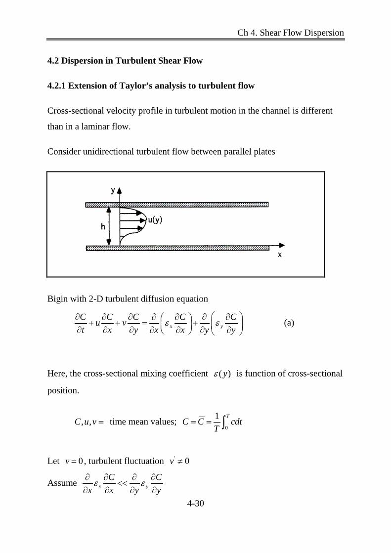
4.2 Dispersion in Turbulent Shear Flow
4.2.1 Extension of Taylor’s analysis to turbulent flow
Cross-sectional velocity profile in turbulent motion in the channel is different
than in a laminar flow.
Consider unidirectional turbulent flow between parallel plates
Bigin with 2-D turbulent diffusion equation
x yC C C C Cu vt x y x x y y
ε ε ∂ ∂ ∂ ∂ ∂ ∂ ∂ + + = + ∂ ∂ ∂ ∂ ∂ ∂ ∂ (a)
Here, the cross-sectional mixing coefficient ( )yε is function of cross-sectional
position.
, ,C u v = time mean values; 0
1 TC C cdt
T= = ∫
Let 0v = , turbulent fluctuation ' 0v ≠
Assume x yC C
x x y yε ε∂ ∂ ∂ ∂
<<∂ ∂ ∂ ∂
Ch 4. Shear Flow Dispersion
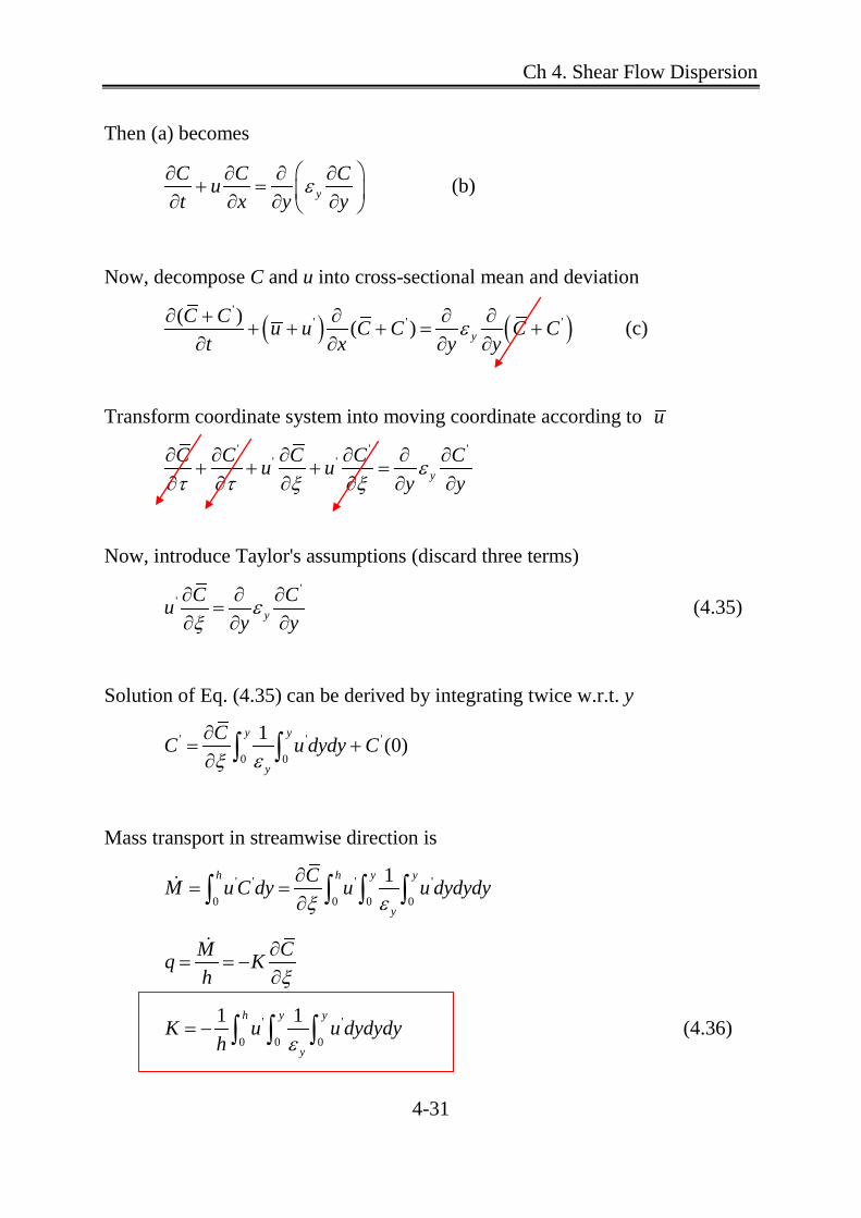
4-31
Then (a) becomes
yC C Cut x y y
ε ∂ ∂ ∂ ∂
+ = ∂ ∂ ∂ ∂ (b)
Now, decompose C and u into cross-sectional mean and deviation
( ) ( )'
' ' '( ) ( ) yC C u u C C C C
t x y yε∂ + ∂ ∂ ∂
+ + + = +∂ ∂ ∂ ∂
(c)
Transform coordinate system into moving coordinate according to u ' ' '
' 'y
C C C C Cu uy yε
τ τ ξ ξ∂ ∂ ∂ ∂ ∂ ∂
+ + + =∂ ∂ ∂ ∂ ∂ ∂
Now, introduce Taylor's assumptions (discard three terms) '
'y
C Cuy yε
ξ∂ ∂ ∂
=∂ ∂ ∂
(4.35)
Solution of Eq. (4.35) can be derived by integrating twice w.r.t. y
' ' '
0 0
1 (0)y y
y
CC u dydy Cξ ε∂
= +∂ ∫ ∫
Mass transport in streamwise direction is
' ' ' '
0 0 0 0
1h h y y
y
CM u C dy u u dydydyξ ε∂
= =∂∫ ∫ ∫ ∫
M Cq Kh ξ
∂= = −
∂
' '
0 0 0
1 1h y y
y
K u u dydydyh ε
= − ∫ ∫ ∫ (4.36)
Ch 4. Shear Flow Dispersion
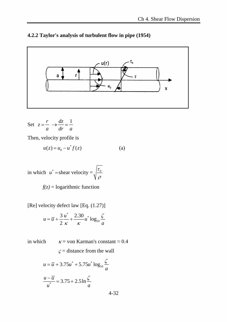
4-32
4.2.2 Taylor's analysis of turbulent flow in pipe (1954)
Set 1r dzza dr a
= → =
Then, velocity profile is *
0( ) ( )u z u u f z= − (a)
in which *u =shear velocity = 0τρ
f(z) = logarithmic function
[Re] velocity defect law [Eq. (1.27)] *
*10
3 2.30 log2
uu u uaζ
κ κ= + +
in which κ = von Karman's constant ≈ 0.4
ς = distance from the wall
* *103.75 5.75 logu u u u
aζ
= + +
* 3.75 2.5lnu uu a
ζ−= +

Ch 4. Shear Flow Dispersion
4-33
The cross-sectional mixing coefficient can be obtained from Reynolds analogy.
→ The mixing coefficients for momentum and mass transports are the same.
i) momentum flux through a surface
ur
τ ερ
∂= −
∂ ☜ Daily & Harleman (p. 56)
ii) mass flux - Fickian behavior
Cqr
ε ∂= −∂
qC ur r
τε∴ = =∂ ∂
− −∂ ∂
(b)
For turbulent flow in pipe, shear stress is given
0 0r za
τ τ τ= = (c)
Differentiate (a) w.r.t. r
* *( ) 1u df z dz dfu ur dz dr dz a∂
= − = −∂
(d)
Divide (c) by (d)
0
* 1z
u dfur dz a
ττ=
∂−
∂
(e)
Kinematic eddy viscosity

Ch 4. Shear Flow Dispersion
4-34
Substitute (e) into (b) *
0 0
* *
( / )1
z az azuu df df dfu ur dz a dz dz
τ τ ρτερ ρ
∴ = − = = =∂∂
Now, it is possible to tabulate ' ( ) ( ) , ( )u r u r u rε= − (f)
And, numerically integrate Eq. (4.39) [Taylor’s equation in radial coordinates]
to obtain ' ( )C r using ( )rε obtained in (f)
2 ' ''
2
1C C Cur r r
εξ
∂ ∂ ∂= + ∂ ∂ ∂
(4.39)
Again, numerically integrate Eq. (4.36) to find K *10.1K au= (4.40)
in which a = pipe radius
( )2*u

Ch 4. Shear Flow Dispersion
4-35
4.2.3 Elder's application of Taylor's method (1959)
Consider turbulent flow down an infinitely wide inclined plane
*' '( ) (1 ln )uu y y
κ= +
assuming von
Karman logarithmic velocity profile
(a)
where *
''
1 1du uu u udy y dκ
= − → = (b)
' /y y d=
d = depth of channel
For open channel flow, shear stress is gives
'0 (1 )du y
dyτ ρε τ= = − (c)
' '' *0 0
*
'
(1 ) (1 )( ) '(1 )1 1
y yy y y dudu udy y d
τ τε κρ ρ
κ
− −= = = − (d)
Substitute Eq. (a) and Eq. (d) into Eq. (4.36) and integrate
'2 2
1
1( ( ) 0.648)n
n
C d d yCx n dκ
∞
=
∂ −= −∂ ∑ (4.44)
*3
0.404K duκ
= (4.45)
Input 0.41κ = *5.93K du= (4.46)
0dudy
=
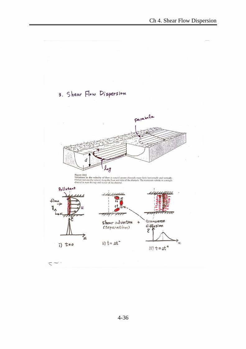
Ch 4. Shear Flow Dispersion
4-36
d

Ch 4. Shear Flow Dispersion
4-37
▪General form for the longitudinal dispersion coefficient
Introduce dimensionless quantities
' ' ',yy y hy dy hdyh
= → = = (a)
''' ' '' '2
2'
uu u u uu
= → = (b)
' 'EEεε ε ε= → = (c)
where E = cross-sectional average of ε 'u = velocity deviation from cross-sectional mean velocity
'2u = 12' 2
0
1 ( )h
u dyh
∫
= intensity of the velocity deviation (different from turbulent intensity)
= measure of how much the turbulent averaged velocity deviates throughout the
cross section from its cross-sectional mean
Substitute (a) ~ (c) into Eq. (4.36) 1 ' ''' '2 '' '2 3 ' ' '
'0 0 0
1 1y yK u u u u h dy dy dy
h Eε= − ∫ ∫ ∫
1 ' ''2 '2 3 '' '' ' ' ''0 0 0
1 1 1y yu u h u u dy dy dy
h E ε= − ∫ ∫ ∫
'2 2 1 ' ''' '' ' ' ''0 0 0
1y yu h u u dy dy dyE ε
= − ∫ ∫ ∫ (d)

Ch 4. Shear Flow Dispersion
4-38
Set 1 ' ''' '' ' ' '
'0 0 0
1y yI u u dy dy dy
ε= −∫ ∫ ∫ (4.48)
Then (d) becomes
2 '2h uK IE
= (4.47)
▪Range of values of I for flows of practical interest
0.054 ~ 0.10I = → 0.10I ≅
Flow Velocity profile
Charac.
length,
h
I K
(i)Laminar flow in a tube 2
0 2(1 )ru ua
= − a 0.0625 2 2
0
192a u
D
(ii)Laminar flow at depth
down on inclined plane
2
0 22 y yu ud d
= −
d 0.0952 2 2
08945
d uD
(iii)Laminar flow with a
linear velocity profile
across a spacing
yu Uh
= h 0.10 2 2
120U h
D
(iv)Turbulent flow in a
pipe empirical a 0.054 *10.1 au
(v)Turbulent flow at
depth down an inclined
plane
*
(1 ln )u yu udκ
= + + d
0.067 *5.93du
Ch 4. Shear Flow Dispersion
4-39
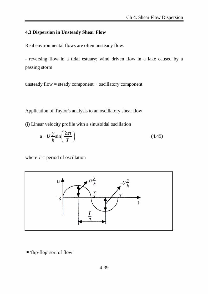
4.3 Dispersion in Unsteady Shear Flow
Real environmental flows are often unsteady flow.
- reversing flow in a tidal estuary; wind driven flow in a lake caused by a
passing storm
unsteady flow = steady component + oscillatory component
Application of Taylor's analysis to an oscillatory shear flow
(i) Linear velocity profile with a sinusoidal oscillation
2siny tu Uh T
π =
(4.49)
where T = period of oscillation
▪'flip-flop' sort of flow

Ch 4. Shear Flow Dispersion
4-40
- reversing instantaneously between yu Uh
= and yu Uh
− = after every time
interval 2T
→ after each reversal the concentration profile has to be reversed
→ substitute – y for y in Eq. (4.21)
→ but enough time bigger than mixing time ( 2 /cT h D≈ ) is required before the
concentration profile is completely adopted to a new velocity profile.
(1) CT T>>
- concentration profile will have sufficient time to adopt itself to the velocity
profile in each direction
- time required for to reach the profile given by Eq.(4.21) is short compared to
the time during which has that profile.
→ dispersion coefficient will be
CT T<<
the same as that in a steady flow
→ dispersion as if flow were steady in either direction
(2)
- period of reversal is very short compared to the cross-sectional mixing time
- concentration profile does not have time to respond to the velocity profile
- 'C will oscillate around the mean of the symmetric limiting profiles, which is 'C =0.
→ dispersion coefficient tends toward zero
→ no dispersion due to the velocity profile

Ch 4. Shear Flow Dispersion
4-41

Ch 4. Shear Flow Dispersion
4-42
▪ Fate of an instantaneous line source when CT T<<
Solution of Eq. (4.13) by Carslaw and Jaeger (1959)
' 2 ''
2
C C CD uyτ ξ
∂ ∂ ∂− = −
∂ ∂ ∂
' 2sin ( 0)y tu u U uh T
π= = =
B.C. '
02
C hat yy
∂= = ±
∂
I.C. '( ,0) 0C y =
Taylor ’s equation for unsteady flow
yu Uh
− =
unsteady source term

Ch 4. Shear Flow Dispersion
4-43
Replace unsteady source term ' Cuξ∂∂
by a source of constant strength
0t t=
by setting
* 2 *
02
2sin( )
tC C y CD Uy h x T
πτ
∂ ∂ ∂− = −
∂ ∂ ∂
*
02
C hat yy
∂= = ±
∂
* ( ,0) 0C y =
where *C = distribution resulting from a suddenly imposed source distribution
of constant strength
As diagrammed in Fig. 2.8, the solution for a series of sources of variable
strength, can be obtained by
' *0 0 00
( , ) ( , ; )t
C y t C y t t t d tt∂
= −∂∫
For large t
' *0 0 0( , ) ( , ; )
tC y t C y t t t d t
t−∞
∂= −
∂∫
*C can be expressed by the sum
*( , ) ( ) ( , )C y t u y w y t= +
( , )w y t can be solved by separation of variables and Fourier expansion.
Further integration of the result leads to

Ch 4. Shear Flow Dispersion
4-44
( )
2'
231
2 ( 1) sin(2 1)2 1
n
nc
Uh T C yC nD T x hn
ππ
∞
=
∂ −= −
∂ −∑
( )1
2 2
2 122 1 1 sin
2 nc
T tnT T
π π θ−
−
× − + +
where ( )
12 2
212 1
1sin 2 1 12n
c
TnT
θ π
−
−−
= − − +
Average over the period of oscillation of K
' '20
2
1 /hT
hCK u C dy h dt
T x−
∂= − ∂
∫ ∫
( )
122 22 22 2
41
2 1 (2 1) 12nc c
U h T Tn nD T T
ππ
−
∞−
=
= − − +
∑
2 2
0
, 0
1,240
c
c
T T K
U hT T KD
<< →→ >> =
[Re] Case of cT T>>
For a linear steady velocity profile, sinyu Uh
α=
2 221 sin
120stU hK
D Dα
=
→ 2 2
01
240U hK
D= is an ensemble average of stK over all values of α
Ch 4. Shear Flow Dispersion
4-45
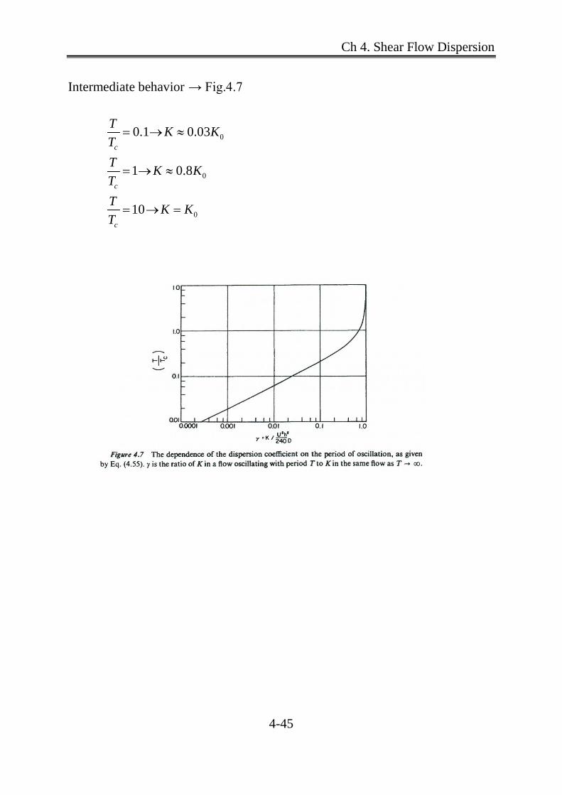
Intermediate behavior → Fig.4.7
0
0
0
0.1 0.03
1 0.8
10
c
c
c
T K KTT K KTT K KT
= → ≈
= → ≈
= → =

Ch 4. Shear Flow Dispersion
4-46
(ii) Flow including oscillating and a steady component
→ pulsating flow found in blood vessel
( ) ( ) ( )1 2sin 2 /u y u y t T u yπ= +
1 2 /u u Uy h= =
Assume that the results by separate velocity profile are additive
' ' '1 2C C C= +
.
Let is solution to ( )' 2 '
2
C C Cu tt x y
ε∂ ∂ ∂+ =
∂ ∂ ∂
Then 1 'C is solution to the equation
' 2 '1 1
1 2sin(2 / )C C Cu t Tt x y
π ε∂ ∂ ∂+ =
∂ ∂ ∂
2 'C is solution to the equation
' 2 '2 2
2 2
C C Cut x y
ε∂ ∂ ∂+ =
∂ ∂ ∂
cycle-averaged dispersion coefficient
' '21 2 1 20
2
1 1 2sin ( )hT
htK u u C C dydt
CT Thx
π−
= − + + ∂ ∂
∫ ∫
' '2 21 1 2 20
2 2
1 1 2sinh hT
h htu C dydt u C dy
C T Thx
π− −
= − + ∂
∂
∫ ∫ ∫
1 2K K= +
where 1K = result of oscillatory profile = ( / )cf T T → Fig. 4.7
2K = result of steady profile

Ch 4. Shear Flow Dispersion
4-47
▪ Application to tidal rivers and estuaries
Consider shear effects in estuaries and tidal rivers
Flow oscillation - flow goes back and forth.
Consider effect of oscillation on the longitudinal dispersion coeff.
0 ( )K K f T ′= (7.1)
where ( )f T ′ is plotted in Fig. 4. 7.
/ cT T T′ = = dimensionless time scale for
T =
cross-sectional mixing
tidal period ∼12 hrs
CT = cross-sectional mixing time = 2 / tW ε
0K = dispersion coefficient if T Tc
• For wide and shallow cross section with no density effects
20 CK Iu T′= (5.17)
where I = dimensionless triple integral 0.1≈ (Table 4.1)
Combine Eq. (7.1) and Eq. (5.17)
( ) ( )20.1 1/K u T T f T′ ′ ′= (7.2)

Ch 4. Shear Flow Dispersion
4-48
Function ( ) ( )1/ T f T′ ′ is plotted in Fig.7.4
i) CT is small (narrow estuary) 2
Ct
WTε
=
1C
TTT
′ = >> → K is small
ii) CT is very large (very wide estuary)
1C
TTT
′ = << → K is smallest
iii) ( ) ( )1 : 1/ 0.8CTT T f TT
′ ′ ′= ≈ ≈
2max 0.08K u T′∴ =
[Ex] 2 212.5 hrs, 0.3 m/s, 0.2T u u u′= = =
2max 0.08 0.2(0.3) (12.5 3600)K = × × × 260 m /s≈
Max = 0.8
Ch. 5

Ch 4. Shear Flow Dispersion
4-49
4.4 Dispersion in Two Dimensions
In many environmental flows velocity vector rotates with depth
( ) ( )u iu z jv z= +
where u = component of velocity u
in the x direction
v = component of velocity u
in the y direction
( )'c z
▽ x u(z) y v(z) z Fig. 4.8 skewed shear flow in the surface layer of Lake Huron
• Taylor’s analysis applied to a skewed shear low with velocity profiles
The 2-D form of Eq. (4.10) for turbulent flow is
'
' 'C C Cu vx y z z
ε∂ ∂ ∂ ∂+ =
∂ ∂ ∂ ∂ (4.61)
'
0Cz
∂=
∂ at 0,z h= (water surface & bottom)
Ch 4. Shear Flow Dispersion
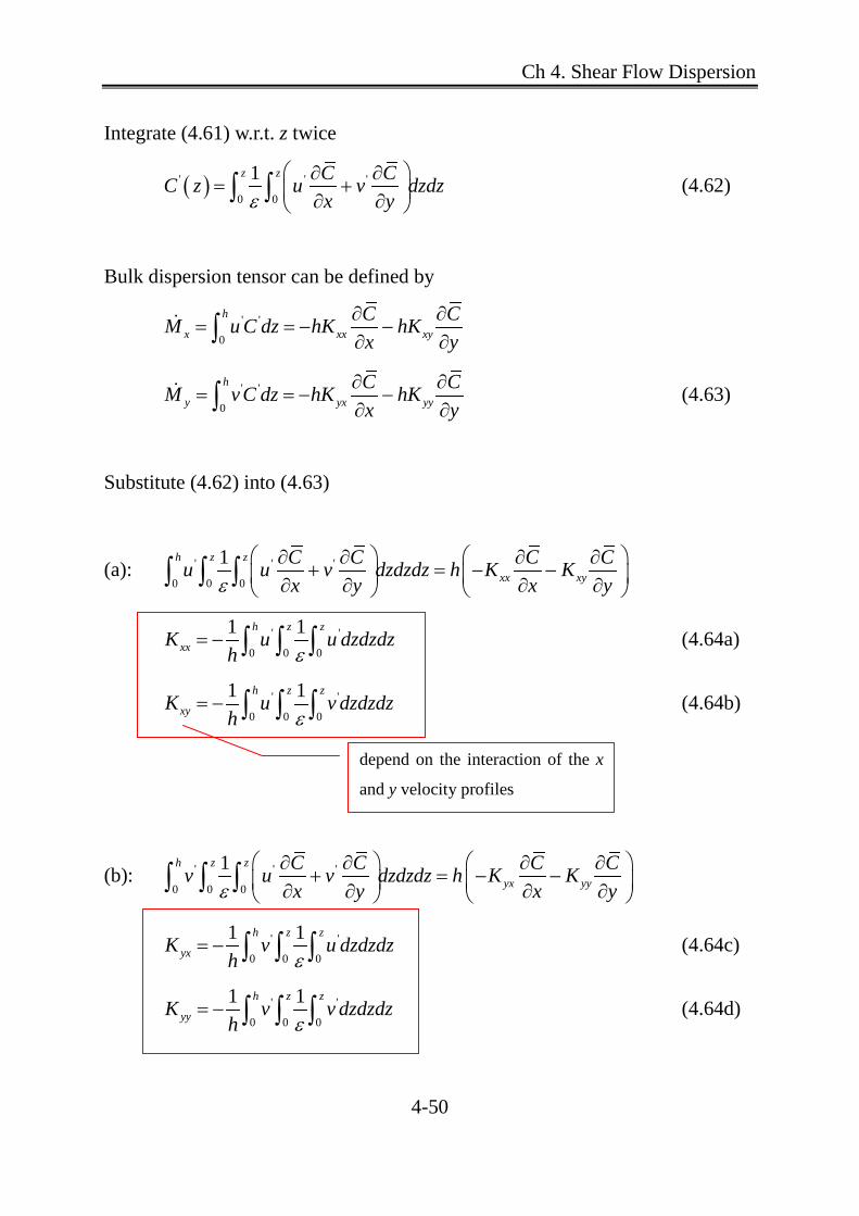
4-50
Integrate (4.61) w.r.t. z twice
( )' ' '
0 0
1z z C CC z u v dzdzx yε
∂ ∂= + ∂ ∂ ∫ ∫ (4.62)
Bulk dispersion tensor can be defined by
' '
0
h
x xx xyC CM u C dz hK hKx y
∂ ∂= = − −
∂ ∂∫
' '
0
h
y yx yyC CM v C dz hK hKx y
∂ ∂= = − −
∂ ∂∫ (4.63)
Substitute (4.62) into (4.63)
(a): ' ' '
0 0 0
1h z z
xx xyC C C Cu u v dzdzdz h K Kx y x yε
∂ ∂ ∂ ∂+ = − − ∂ ∂ ∂ ∂
∫ ∫ ∫
' '
0 0 0
1 1h z z
xxK u u dzdzdzh ε
= − ∫ ∫ ∫ (4.64a)
' '
0 0 0
1 1h z z
xyK u v dzdzdzh ε
= − ∫ ∫ ∫ (4.64b)
(b): ' ' '
0 0 0
1h z z
yx yyC C C Cv u v dzdzdz h K Kx y x yε
∂ ∂ ∂ ∂+ = − − ∂ ∂ ∂ ∂
∫ ∫ ∫
' '
0 0 0
1 1h z z
yxK v u dzdzdzh ε
= − ∫ ∫ ∫ (4.64c)
' '
0 0 0
1 1h z z
yyK v v dzdzdzh ε
= − ∫ ∫ ∫ (4.64d)
depend on the interaction of the x
and y velocity profiles

Ch 4. Shear Flow Dispersion
4-51
The velocity gradient in the x direction can produce mass transport in the y
direction and vice versa.
xyK = x-dispersion coefficient due to velocity gradient in the y direction
yxK = y-dispersion coefficient due to velocity gradient in the x direction
▪ Mean flow on a continental shelf (Fischer, 1978)
y (offshore)
0v V=
x (alongshare)
2d u
z=d 0U 0v V= −
22
0 0 0
20 0 0
/ 120 5 /192
5 /192 /120
U U VdKU V Uε
=
(4.65)
1.2km y 5t days= 5 /u cm s= x=22km 0 5 /U cm s= ( )ut= 72.6° 0 5 /V cm s= x 28 km Source
Distribution of concentrated slug of dye after 5 days

Ch 4. Shear Flow Dispersion
4-52
[Re] Derivation of 2-D dispersion equation yq x xq dx dy x
xqq xx
∂+ ∆∂
y y
y
qq y
y∂
+ ∆∂
(i) Conservation of mass
yxx x y y
qC qx y q q x y q q y xt x y
∂ ∂ ∂ ∆ ∆ = − + ∆ ∆ + − + ∆ ∆ ∂ ∂ ∂
yx qC qt x y
∂∂ ∂∴ = − −
∂ ∂ ∂ (1)
(ii) Apply Taylor’s Analysis on 2-D shear flow
( )' ' ' ' ' ' '
0
1h
x xC Cq M u C h u C dz u u v dzdzdzx yε
∂ ∂= = = = + ∂ ∂
∫ ∫ ∫ ∫
xx xyC CK Kx y
∂ ∂= − −
∂ ∂ (2)
( )' ' ' ' ' ' '
0
1h
y yC Cq M v c h v c dz v u v dzdzdzx yε
∂ ∂= = = = + ∂ ∂
∫ ∫ ∫ ∫
yx yyC CK Kx y
∂ ∂= − −
∂ ∂ (3)
(iii) Substitute (2) & (3) into (1)
xx xy yx yyC C C C CK K K Kt x x y y x y
∂ ∂ ∂ ∂ ∂ ∂ ∂= − − − − − − ∂ ∂ ∂ ∂ ∂ ∂ ∂

Ch 4. Shear Flow Dispersion
4-53
(iv) Return to fixed coordinate system containing mean advective velocities
xx xy yx yyC C C C C C Cu v K K K Kt x y x x y y x y
∂ ∂ ∂ ∂ ∂ ∂ ∂ ∂ ∂+ + = + + + ∂ ∂ ∂ ∂ ∂ ∂ ∂ ∂ ∂
In general xyK and yxK are small compared with xxK and yyK . Thus, those
two terms are often neglected. Then, 2-D depth-averaged transport equation
becomes
xx yyC C C C Cu v K Kt x y x x y y
∂ ∂ ∂ ∂ ∂ ∂ ∂ + + = + ∂ ∂ ∂ ∂ ∂ ∂ ∂
[Cf] 2-D depth-averaged models (ASCE, 1988; vol.114, No.9)
∙ Scalar transport equation forΦ
( ) ( ) ( ) ( ) ( )1 1x y
HU HVHHJ HJ
t x y x yρ ρ∂ Φ ∂ Φ∂ Φ ∂ ∂
+ + = +∂ ∂ ∂ ∂ ∂
' ' ' '1 1
dispersion dispersion
U dz V dzx y
ρ ρρ ρ∂ ∂
+ Φ + Φ∂ ∂∫ ∫
where ' 'xJ u dzρ φ= −∫ turbulent diffusion in x-dir
' 'yJ u dzρ φ= −∫ turbulent diffusion in y-dir
'u u U= − → time fluctuation
'φ φ= −Φ

Ch 4. Shear Flow Dispersion
4-54
'U U U= − → depth deviation
'Φ =Φ −Φ
If dispersion >> turbulent diffusion
→ neglect turbulent diffusion or incorporate turbulent diffusion into dispersion.


![편경영과학적방법론 - ocw.snu.ac.krocw.snu.ac.kr/sites/default/files/NOTE/2288.pdf선형계획모형(2) 선형계획문제의특징 [1] 목적함수와제약조건들이변수의선형관계로표현된다](https://img.dokumen.tips/doc/110x75/5e4ffd96fb45fe01ca1702d8/eeeee-ocwsnuackrocwsnuackrsitesdefaultfilesnote2288pdf.jpg)