Embed Size (px)
Citation preview

Ocean wave measurements by TerraSAR-X Waves Travelling into Sea Ice
East Greenland Case S. Lehner, J. Gemmrich, A. Pleskachevsky, C.Gebhardt J. Bidlot, W. Rosenthal

2007
2010
Stripmap 30km ScanSAR 100km Wide ScanSAR 250km SpotLight 10km
1m Resolution
3m Resolution
16m Resolution
35m Resolution
10km
-Radar signal penetrates clouds -No sun light is necessary
Wide ScanSAR: 35m resolution StripMap: 3m resolution
Satellites: X-band SAR (Synthetic Aperture Radar) TerraSAR-X and TanDEM-X

Sea State and Eddies at the Sea Ice Boundary
30 km x 50 km subscene
Sequence of TS-X images off the coast of Eastern Greenland, strip 300 km acquired on Feb.5th,2013, 8:40 UTC, From top to bottom, typical signatures of -ice floes and solid ice, -pancake ice, -frazil ice (dark)


Page

Page


Left: Stripmap image which is part of the TS-X scene shown . Right: Classification of ice types for the image shown on the left. Blue is open water/nilas, magenta is young ice, bright green is thin first year ice, and dark green is thick first year ice.

wave spectra from ECMWF long and short/young swell consistent with TS-X shown
Wave Model Spectrum ECMWF
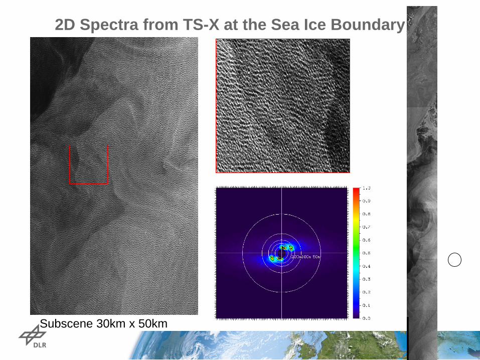
2D Spectra from TS-X at the Sea Ice Boundary
Subscene 30km x 50km

Fourier power spectrum showing 2 maxima: swell waves of more than 300 m length travelling close to azimuth direction, shorter waves of ca. 180 m length travelling more in range direction
Maxima of TS-X Spectrum

peak wavelength of 358 m and 367 m, travelling to NE
TS-X Cross Spectrum Swell Peak of > 300 m waves

Peak Wavelength of SW travelling ~ 180 m Waves

swell waves of 150 to 200 m length travelling in South-western direction, Again velocity dispersion is observed
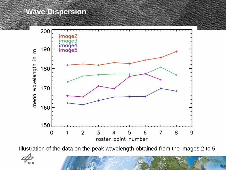
Illustration of the data on the peak wavelength obtained from the images 2 to 5.
Wave Dispersion

Velocity Dispersion of Swell at a fixed time (contrary to a fixed place)
For storm distance D to the location of measurement there is the relation For wave length L, group velocity v and travel time τ we have the relation: D (L, τ) = v(L) τ = 0.5 sqrt(1.56 * L) τ = 0.63 sqrt(L) τ (1) For wave length L and fixed τ , the distance D changes dD/dL = 0.32 τ / sqrt (L). (2) For the considered case in open water we measure typical values dD/dL~ 1000. That gives the travel distance from (2) for L=400 m: τ = 3.12 *sqrt (L) (dL/dx)-1 ~ 3.12 * sqrt(400) * 1000 = 62 400 s. The distance D from the storm center is D =1600 km For the short peak L = 200m a similar calculation gives D = 372 km. In Snodgrass et all : „Swell across the Pacific“, a similar relation was derived to explain the shift of peak frequency for anchored wave sensors (at a fixed place).

Wave Length change due to ice sheet Thickness (after Wadhams and Squire)
is recommended by Squire et al (1995). h is the thickness of the ice sheet. Wadhams massload approximation is (g/ ω2 - λ / (2 π)) = hρ´/ρ For constant ω the differences in h for two locations are proportional to differences in λ :
(λ0 − λ)(ρ´/ρ) / (2π) = dh = h – h0
In a continuos sheet of sea ice floating in infinite deep water the dispersion relation


Swh starts from 3-4 m in the South in free open ocean Decreases below 1m in the ice Largest gradient of swh on the left Dark appearance of grease ice on SAR image on the right are clearly related to Hs
Significant Wave Height at the Sea Ice Boundary
XWAVE_Coast_1.9

Summary and Conclusions -Spatial Ocean Wave Measurements over 300 km x 30 km between Greenland and Iceland in February 2013 -Measurements of 2D Spectra, Peak Wavelength and Direction, Significant Wave Height - Comparison to ECMWF Wave Model -Velocity Dispersion observable – leads to estimation of storm distance and ice thickness -2 Peaks observed, with wave length 380m and 180m -Measurement of behaviour in sea ice