Ocean carbon and nitrogen isotopes in CSIRO Mk3L-COAL ... · The CSIRO Mk3L-COAL couples a computationally efﬁ-cient climate system model (Phipps et al.,2013) with bio-geochemical

Geosci. Model Dev., 12, 1491–1523, 2019https://doi.org/10.5194/gmd-12-1491-2019© Author(s) 2019. This work is distributed underthe Creative Commons Attribution 4.0 License.

Ocean carbon and nitrogen isotopes in CSIRO Mk3L-COALversion 1.0: a tool for palaeoceanographic researchPearse J. Buchanan1,2,3,a, Richard J. Matear2,3, Zanna Chase1, Steven J. Phipps1, and Nathan L. Bindoff1,2,3,4

1Institute for Marine and Antarctic Studies, University of Tasmania, Hobart, Tasmania, Australia2CSIRO Oceans and Atmosphere, CSIRO Marine Laboratories, G.P.O. Box 1538, Hobart, Tasmania, Australia3ARC Centre of Excellence in Climate System Science, Hobart, Tasmania, Australia4Antarctic Climate and Ecosystems Cooperative Research Centre, Hobart, Tasmania, Australiaanow at: the Department of Earth, Ocean and Ecological Sciences, University of Liverpool, Liverpool, UK

Correspondence: Pearse J. Buchanan ([email protected])

Received: 11 September 2018 – Discussion started: 27 November 2018Revised: 22 March 2019 – Accepted: 26 March 2019 – Published: 16 April 2019

Abstract. The isotopes of carbon (δ13C) and nitrogen (δ15N)are commonly used proxies for understanding the ocean.When used in tandem, they provide powerful insight intophysical and biogeochemical processes. Here, we detail theimplementation of δ13C and δ15N in the ocean component ofan Earth system model. We evaluate our simulated δ13C andδ15N against contemporary measurements, place the model’sperformance alongside other isotope-enabled models anddocument the response of δ13C and δ15N to changes inecosystem functioning. The model combines the Common-wealth Scientific and Industrial Research Organisation Mark3L (CSIRO Mk3L) climate system model with the Carbonof the Ocean, Atmosphere and Land (COAL) biogeochemi-cal model. The oceanic component of CSIRO Mk3L-COALhas a resolution of 1.6◦ latitude× 2.8◦ longitude and resolvesmultimillennial timescales, running at a rate of ∼ 400 yearsper day. We show that this coarse-resolution, computation-ally efficient model adequately reproduces water column andcore-top δ13C and δ15N measurements, making it a usefultool for palaeoceanographic research. Changes to ecosystemfunction involve varying phytoplankton stoichiometry, vary-ing CaCO3 production based on calcite saturation state andvarying N2 fixation via iron limitation. We find that largechanges in CaCO3 production have little effect on δ13C andδ15N, while changes in N2 fixation and phytoplankton sto-ichiometry have substantial and complex effects. Interpre-tations of palaeoceanographic records are therefore open tomultiple lines of interpretation where multiple processes im-print on the isotopic signature, such as in the tropics, where

denitrification, N2 fixation and nutrient utilisation influenceδ15N. Hence, there is significant scope for isotope-enabledmodels to provide more robust interpretations of the proxyrecords.

1 Introduction

Elements that are involved in reactions of interest, such asexchanges of carbon and nutrients, experience isotopic frac-tionation. Typically, the heavier isotope will be enrichedin the reactant during kinetic fractionation, in more oxi-dised compounds during equilibrium fractionation and in thedenser form during phase state fractionation (i.e. evapora-tion). Because fractionation against one isotope relative tothe other is minuscule, the isotopic content of a sample isconventionally expressed as a δ value (δhE), where the ratioof the heavy to light element in solution (hE:lE) is comparedto a standard ratio (hEstd:

lEstd) in units of per mille (‰).

δhE =

( hE : lEhEstd : lEstd

− 1)· 1000 (1)

The strength of fractionation against the heavier isotopeduring a given reaction, ε, is also expressed in per millenotation. Fractionation with an ε equal to 10 ‰, for exam-ple, will involve 990 units of hE for every 1000 units oflE at a hypothetical standard ratio (hEstd:

lEstd) of 1 : 1. Atmore realistic standard ratios ≪1 : 1, say 0.0112372 : 1 fora δ13C value of 0 ‰, a fractionation at 10 ‰ would involve

Published by Copernicus Publications on behalf of the European Geosciences Union.

1492 P. J. Buchanan et al.: Ocean δ13C and δ15N in CSIRO Mk3L-COAL v1.0

∼ 0.0111123(

0.010 · 0.01123721.0112372

)units of 13C per unit of 12C.

Slightly greater preference of one isotope over another inthis case involves a preference for the lighter carbon isotope(12C) over the heavier (13C), which enriches the remainingdissolved inorganic carbon (DIC) in 13C and depletes theproduct. Certain isotopic preferences, or strengths of frac-tionation, therefore allow certain reactions to be detected inthe environment.

The measurement of the stable isotopes of carbon (δ13C)and nitrogen (δ15N) have been fundamental for understand-ing how these important elements cycle within the ocean (e.g.Schmittner and Somes, 2016; Menviel et al., 2017a; Rafteret al., 2017; Muglia et al., 2018). We will now briefly intro-duce each isotope in turn.

The distribution of δ13C is dependent on air–sea gas ex-change, ocean circulation and organic matter cycling. Thesecontributions make the δ13C signature difficult to interpret,and several modelling studies have attempted to elucidatetheir roles (Tagliabue and Bopp, 2008; Schmittner et al.,2013). These studies have shown that preferential uptake of12C over 13C by biology in surface waters enforces stronghorizontal and vertical gradients in δ13C of DIC (δ13CDIC),greatly enriching surface waters, particularly in subtropi-cal gyres where vertical exchange with deeper waters is re-stricted (Tagliabue and Bopp, 2008; Schmittner et al., 2013).Meanwhile, air–sea gas exchange and carbon speciation con-trol the δ13CDIC reservoir over longer timescales (Schmittneret al., 2013). Because air–sea and speciation fractionationare temperature dependent, such that cooler conditions tendto elevate the δ13CDIC of surface waters, they also tend tosmooth the gradients produced by biology by working antag-onistically to them. Despite this smoothing, biological frac-tionation drives strong gradients at the surface, which im-parts unique δ13C signatures to the water masses that arecarried into the interior. These insights have provided clearevidence of reduced ventilation rates in the deep ocean dur-ing glacial climates (Tagliabue et al., 2009; Menviel et al.,2017a; Muglia et al., 2018).δ15N is determined by biological processes that add or re-

move fixed forms of nitrogen. It therefore records the rel-ative rates of sources and sinks within the marine nitrogencycle (Brandes and Devol, 2002). Dinitrogen (N2) fixation isthe largest source of fixed nitrogen to the ocean, the bulk ofwhich occurs in warm, sunlit surface waters and introducesnitrogen with a δ15N of approximately −1 ‰ (Sigman et al.,2009). Denitrification is the largest sink of fixed nitrogenand occurs in deoxygenated water columns and sediments.Denitrification fractionates strongly against 15N at ∼ 25 ‰(Cline and Kaplan, 1975). Fractionation during denitrifica-tion is most strongly expressed in the water column whereample nitrate (NO3) is available, making water column den-itrification responsible for elevating global mean δ15N abovethe −1 ‰ of N2 fixers (Brandes and Devol, 2002). Mean-while, denitrification occurring in the sediments only weakly

fractionates against 15N (Sigman et al., 2009), providing onlya slight enrichment of δ15N above that introduced by N2 fix-ation. Variations in δ15N can therefore tell us about globalchanges in the ratio of sedimentary to water column denitri-fication, with increases in δ15N associated with increases inthe proportion of denitrification occurring in the water col-umn (Galbraith et al., 2013), but it can also reflect regionalchanges in N2 fixation and denitrification (Ganeshram et al.,1995; Ren et al., 2009; Straub et al., 2013).

However, nitrogen isotopes are also subject to the effectof utilisation, which makes the interpretation of δ15N morecomplicated. Basically, when nitrogen is abundant, the pref-erence for 14N over 15N increases but when nitrogen is lim-ited this preference disappears (Altabet and Francois, 2001).Complete utilisation of nitrogen therefore reduces fractiona-tion to 0 ‰. While this adds complexity, it also imbues δ15Nas a proxy of nutrient utilisation by phytoplankton. As nitro-gen supply to phytoplankton is controlled by physical de-livery from below, changes in δ15N can be interpreted aschanges in the physical supply (Studer et al., 2018). Phy-toplankton fractionate against 15N at ∼ 5 ‰ (Wada, 1980)when bioavailable nitrogen is abundant. If nitrogen is utilisedto completion, which occurs in much of the low to midlat-itude ocean, then no fractionation will occur and the δ15Nof organic matter will reflect the δ15N of the nitrogen thatwas supplied (Sigman et al., 2009). However, in the casewhere nitrogen is not consumed towards completion, whichoccurs in zones of strong upwelling/mixing near coastlines,the Equator and high latitudes, the bioavailable nitrogen poolwill be enriched in 15N as phytoplankton preferentially con-sume 14N. As the remaining bioavailable N is continually en-riched in 15N, the organic matter that settles into sedimentsbeneath a zone of incomplete nutrient utilisation will bearthis enriched δ15N signal. In combination with modelling(Schmittner and Somes, 2016), the δ15N record is able toprovide evidence for a more efficient utilisation of bioavail-able nitrogen during glacial times (Martinez-Garcia et al.,2014; Kemeny et al., 2018) and a less efficient one duringthe Holocene (Studer et al., 2018).

Complimentary measurements of δ13C and δ15N providepowerful, multi-focal insights into oceanographic processes.δ13C is largely a reflection of how water masses mix awaythe strong vertical and horizontal gradients enforced by biol-ogy, while δ15N simultaneously reflects changes in the ma-jor sources and sinks of the marine nitrogen cycle and howeffectively nutrients are consumed at the surface. However,the interpretation of these isotopes is often difficult. They aresubject to considerable uncertainty because there are multi-ple processes that imprint on the measured values. Our goalis to equip version 1.0 of the Commonwealth Scientific andIndustrial Research Organisation Mark 3L (CSIRO Mk3L)climate system model with the Carbon of the Ocean, Atmo-sphere and Land (COAL) Earth system model with oceanicδ13C and δ15N such that this model can be used for in-terpreting palaeoceanographic records. First, we introduce

Geosci. Model Dev., 12, 1491–1523, 2019 www.geosci-model-dev.net/12/1491/2019/

P. J. Buchanan et al.: Ocean δ13C and δ15N in CSIRO Mk3L-COAL v1.0 1493

CSIRO Mk3L-COAL. Second, we detail the equations thatgovern the implementation of carbon and nitrogen isotopes.Third, we assess our simulated isotopes against contempo-rary measurements from both the water column and sed-iments and compare the model performance against otherisotope-enabled models. Finally, as a first test of the model,we take the opportunity to document how changes in ecosys-tem functioning affect δ13C and δ15N.

2 CSIRO Mk3L-COAL v1.0

The CSIRO Mk3L-COAL couples a computationally effi-cient climate system model (Phipps et al., 2013) with bio-geochemical cycles in the ocean, atmosphere and land. Themodel is therefore based on the CSIRO Mk3L climate sys-tem model, where the “L” denotes that it is a low-resolutionversion of the CSIRO Mk3 model that contributed towardsthe third phase of Coupled Model Intercomparison Project(Meehl et al., 2007) and the Fourth Assessment Report ofthe Intergovernmental Panel on Climate Change (Solomonet al., 2007). See Smith (2007) for a complete discussion ofthe CSIRO family of climate models. The land biogeochem-ical component represents carbon, nitrogen and phospho-rus cycles in the Community Atmosphere Biosphere LandExchange (CABLE) (Mao et al., 2011). The ocean compo-nent currently represents carbon, alkalinity, oxygen, nitro-gen, phosphorus and iron cycles. The atmospheric compo-nent conserves carbon and alters its radiative properties ac-cording to changes in its carbon content. For this paper, wefocus on the ocean biogeochemical model (OBGCM).

Previous versions of the OBGCM have explored changesin oceanic properties under past (Buchanan et al., 2016),present (Buchanan et al., 2018) and future scenarios (Matearand Lenton, 2014, 2018). These studies demonstrate that themodel can reproduce observed features of the global car-bon cycle, nutrient cycling and organic matter cycling in theocean. The OBGCM offers highly efficient simulations ofthese processes at computational speeds of ∼ 400 years perday when the ocean general circulation model (OGCM) isrun offline (compared to ∼ 10 years per day in fully coupledmode). The ocean is made up of grid cells of 1.6◦ in latitudeby 2.8◦ in longitude, with 21 vertical depth levels spaced by25 m at the surface and 450 m in the deep ocean (Table 1).The OGCM time step is 1 h, while the OBGCM time step is1 d. The ability of the OBGCM to reproduce large-scale dy-namical and biogeochemical properties of the ocean coupledwith its fast computational speed makes the OBGCM usefulas a tool for palaeoceanographic research.

2.1 Ocean biogeochemical model (OBGCM)

The OBGCM is equipped with 13 prognostic tracers (Fig. 1).These can be grouped into carbon chemistry fields, oxygenfields, nutrient fields, age tracers and nitrous oxide (N2O).

Carbon chemistry fields include DIC, alkalinity (ALK),DI13C and radiocarbon (14C). Radiocarbon is simulated ac-cording to Toggweiler et al. (1989). Oxygen fields includedissolved oxygen (O2) and abiotic dissolved oxygen (Oabio

2 ),a purely physical tracer from which true oxygen utilisation(TOU) can be calculated (Duteil et al., 2013). Nutrient fieldsinclude phosphate (PO4), dissolved bioavailable iron (Fe),nitrate (NO3) and 15NO3. Although we define the phospho-rus and nitrogen tracers as their dominant species, being PO4and NO3, these tracers can also be thought of as total dis-solved inorganic phosphorus and nitrogen pools. Reminer-alisation, for instance, implicitly accounts for the processof nitrification from ammonium (NH4) to NO3 (Paulmieret al., 2009) and therefore implicitly includes NH4 and ni-trite (NO2) within the NO3 tracer. Age tracer fields includeyears since subduction from the surface (Agegbl) and yearssince entering a suboxic zone where O2 concentrations areless than 10 mmol m−3 (Ageomz). Finally, N2O in µmolm−3

is produced via nitrification and denitrification according tothe temperature-dependent equations of Freing et al. (2012).All air–sea gas exchanges (CO2, 13CO2, O2 and N2O) andcarbon speciation reactions are computed according to theOcean Modelling Intercomparison Project phase 6 protocol(Orr et al., 2017).

Because the isotopes of carbon and nitrogen are influencedby biological processes and there is as yet no accepted stan-dard for ecosystem model parameterisation in the community(see Hülse et al., 2017, for a more detailed discussion), weprovide a thorough description of the ecosystem componentof the OBGCM in Sect. A in the Appendix. Default param-eters for the OBGCM are further provided in Sect. B in theAppendix. Briefly, the ecosystem model simulates the pro-duction, remineralisation and stoichiometry (elemental com-position) of three types of primary producers: a general phy-toplankton group, diazotrophs (N2 fixers) and calcifiers.

3 Carbon and nitrogen isotope equations

3.1 δ13C

The OBGCM explicitly simulates the fractionation of 13Cfrom the total DIC pool, where for simplicity we make theassumption that the total DIC pool represents the light iso-tope of carbon and is therefore DI12C. Fractionation occursduring air–sea gas exchange, equilibrium reactions and bio-logical consumption in the euphotic zone.

The air–sea gas exchange of 13CO2 is calculated as the ex-change of CO2 with additional fractionation factors appliedto the sea–air and air–sea components (Zhang et al., 1995;Orr et al., 2017). The flux of 13CO2 across the air–sea inter-face, F(13CO2), therefore takes the form of CO2 with addi-tional terms that convert to units of 13C in both environments.Without any isotopic fractionation, the equation requires thegas piston velocity of carbon dioxide in m s−1 (kCO2 ), the

www.geosci-model-dev.net/12/1491/2019/ Geosci. Model Dev., 12, 1491–1523, 2019


Figure 1. A conceptual representation of the ocean biogeochemical model (OBGCM). The bottom panel shows organic matter cycling in-volving the isotopes of carbon and nitrogen. (1) Carbon chemistry reactions. (2) Air–sea gas exchange. (3) Biological uptake of nutrientsand production of organic and inorganic matter. Particulate organic carbon (POC) is produced by the general phytoplankton group and N2fixers (diazotrophs), while particulate inorganic carbon (PIC) as calcium carbonate (CaCO3) is produced by calcifiers. Export of POC by thegeneral (G) phytoplankton group and N2 fixers (D; diazotrophs) is herein referred to as CG

org and CDorg (see Sect. A1 in the Appendix), respec-

tively. (4) Remineralisation of sinking organic matter under oxic and suboxic conditions. (5) Sedimentary oxic and suboxic remineralisation.(6) Nitrous oxide production and consumption.

concentration of aqueous CO2 in both mediums at the air–sea interface in mmol m−3 (COair

2 and COsea2 ) and the ratios

of 13C:12C in both mediums (Ratm and Rsea):

F(13CO2)= kCO2 ·

(COair

2 ·Ratm − COsea2 ·RDIC

), (2)

where

RDIC =DI13C

DI13C+DI12C

Ratm =13CO2

13CO2+ 12CO2= 0.011164381.

A transfer of 13C into the ocean is therefore positive and anoutgassing is negative. The Ratm is set to a preindustrial at-mospheric δ13C of −6.48 ‰ (Friedli et al., 1986).

The fractionation of carbon isotopes during air–sea ex-change involves three components. These are (ε

13Ck ), a ki-

netic fractionation that occurs during transfer of gaseous CO2

into or out of the ocean; (ε13Caq←g), a fractionation that oc-



curs as gaseous CO2 becomes aqueous CO2 (is dissolved insolution); and (ε

13CDIC←g), an equilibrium isotopic fractiona-

tion as carbon speciates into DIC constituents (H2CO2 ⇔

HCO−3 ⇔ CO2−3 ). The kinetic fractionation during transfer,

ε13Ck , is constant at 0.99912, thus reducing the δ13C of car-

bon entering the ocean by 0.88 ‰. Conversely, carbon out-gassing increases the δ13C of the ocean. The fractionationsduring dissolution (ε

13Caq←g) and speciation (ε

13CDIC←g) are both

dependent on temperature. Fractionation during speciation isalso dependent on the fraction of CO2−

3 relative to total DIC(fCO2−

3). These fractionation factors are parameterised as

ε13Caq←g =

0.0049 · T − 1.311000

+ 1 (3)

ε13CDIC←g =

0.0144 · T · fCO2−3− 0.107 · T + 10.53

1000+ 1. (4)

Dissolution of CO2 into seawater (ε13Caq←g) therefore prefer-

ences the lighter isotope and lowers δ13C by between 1.32 ‰and 1.14 ‰, while the speciation of gaseous CO2 into DICinstead prefers the heavier isotope and raises δ13C by be-tween 10.7 ‰ and 6.8 ‰ for temperatures between −2 and35 ◦C.

These fractionation factors are applied to the gaseous ex-change of CO2 (Eq. 2) to calculate carbon isotopic fraction-ation.

F(13CO2)= k · ε13Ck · ε

13Caq←g

·

(COair

2 ·Ratm −COsea

2 ·RDIC

ε13CDIC←g

)(5)

Because fractionation to aqueous CO2 from DIC (ε13Caq←DIC)

is equal toε

13Caq←g

ε13CDIC←g

, a strong preference to hold the heavy iso-

tope in solution exists (ε13Caq←DIC =−11.9 ‰ to −7.9 ‰ be-

tween −2 and 35 ◦C). Aqueous carbon that is transferred tothe atmosphere is hence depleted in 13C. It is therefore theequilibrium fractionation associated with carbon speciationthat is largely responsible for bolstering the oceanic δ13C sig-nature above the atmospheric signature, as it tends to shift13C towards the oxidised species (CO2−

3 ), a tendency thatstrengthens under cooler conditions.

In the default version of CSIRO Mk3L-COAL v1.0, thefractionation of carbon during biological uptake (ε

13Cbio ) is set

at 21 ‰ for general phytoplankton, 12 ‰ for diazotrophs(e.g. Carpenter et al., 1997) and at 2 ‰ for the formation ofcalcite (Ortiz et al., 1996). However, a variable fractionationrate for the general phytoplankton group may be activatedand depends on the aqueous CO2 concentration (CO2(aq)in mmol m−3) and the growth rate (µ in d−1, as a functionof temperature and limiting resources) following Tagliabueand Bopp (2008):

ε13Cbio =

(0.371−

µ

CO2(aq)

)/0.015. (6)

An upper bound of 25 ‰ exists within Eq. (6) when µCO2(aq)

approaches zero but a lower bound does not. We chose tolimit ε

13Cbio to a minimum of 15 ‰ given the reported varia-

tions of ε13Cbio from culture studies (e.g. Laws et al., 1995).

ε13Cbio =max

(15,ε

13Cbio

)(7)

Biological fractionation of 13C is then applied to the uptakeand release of organic carbon.

1DI13C= RDIC ·Corg ·(

1−ε

13Cbio

1000

)(8)

Because biological fractionation is strong for the generalphytoplankton group, which dominates export productionthroughout most of the ocean, this imparts a negative δ13Csignature to the deep ocean. Subsequent remineralisation re-leases DIC with no fractionation. Finally, the concentrationof DI13C is converted into a δ13C via

δ13C=(

DI13CDIC

·1

0.0112372− 1

)· 1000, (9)

where 0.0112372 is the Pee Dee Belemnite standard (Craig,1957).

3.2 δ15N

The OBGCM explicitly simulates the fractionation of 15Nfrom the pool of bioavailable nitrogen. For simplicity, wetreat this bioavailable pool as nitrate (NO3), where total NO3is the sum of 15NO3 and 14NO3. We therefore chose to ignorefractionation during reactions involving ammonium, nitriteand dissolved organic nitrogen, which can vary in their iso-topic composition independent of NO3 but represent a smallfraction of the bioavailable pool of nitrogen.

The isotopic signatures of N2 fixation and atmospheric de-position, and the fractionation during water column denitri-fication (ε

15Nwc ) and sedimentary denitrification (ε

15Nsed ) deter-

mine the global δ15N of NO3 (Brandes and Devol, 2002).Biological assimilation (ε

15Nbio ) and remineralisation are inter-

nal exchanges of the oceanic nitrogen cycle and affect thedistribution of δ15NO3. N2 fixation and atmospheric deposi-tion introduce 15NO3 to the ocean with δ15N values of−1 ‰and −2 ‰, respectively, while biological assimilation, watercolumn denitrification and sedimentary denitrification frac-tionate against 15NO3 at 5 ‰, 20 ‰ and 3 ‰, respectively(Sigman et al., 2009, Fig. 1).

The accepted standard 15N:14N ratio used to measure vari-ations in nature is the average atmospheric 15N:14N ratioof 0.0036765. To minimise numerical errors caused by theOGCM, we set the atmospheric standard to 1. This scales upthe 15NO3 such that a δ15N value of 0 ‰ was equivalent to a15N:14N ratio of 1 : 1.

Because we simulate NO3 and 15NO3 as tracers, our calcu-lations require solving for an implicit pool of 14NO3 during



each reaction involving 15NO3. The introduction of NO3 ata fixed δ15NNO3 of −1 ‰ due to remineralisation of N2 fixerbiomass provides a simple example with which we can beginto describe our equations. Setting the isotopic value of newlyfixed NO3 to−1 ‰ is simple because it removes any compli-cations associated with fractionation. We note, however, thatin reality the nitrogenase enzyme does fractionate during itsconversion of aqueous N2 (+0.7 ‰) to ammonium and thebiomass that is subsequently produced can vary substantiallydepending of the type of nitrogenase enzyme used (vanadiumversus molybdenum based) (McRose et al., 2019). However,we choose to implicitly account for these transformations andconsiderably simplify them by setting the δ15N of N2 fixerbiomass equal to −1 ‰, which reflects the biomass of N2fixers associated with the more common Mo-nitrogenase.

A δ15NNO3 of −1 ‰ is equivalent to a 15N:14N ratio of0.999 in our approach, where 0 ‰ equals a 1 : 1 ratio of15N:14N. If the amount of NO3 being added is known along-side its 15N:14N ratio, in this case 0.999 for N2 fixation, weare able to calculate how much 15NO3 is added. We beginwith two equations that describe the system.

NO3 =15NO3+

14NO3 (10)

δ15NNO3 =

( 15NO3/14NO3

15Nstd/14Nstd− 1

)· 1000 (11)

Ultimately, we need to solve for the change in 15NO3 associ-ated with an introduction of NO3 by N2 fixation. Our knownvariables are the change in NO3, the δ15N of that NO3 andthe 15Nstd/

14Nstd. Our two unknowns are 15NO3 and 14NO3.We must solve for 14NO3 implicitly by describing it accord-ing to 15NO3 by rearranging Eq. (11).

14NO3 =15NO3/

((δ15NNO3

1000+ 1

)·

15Nstd/14Nstd

)(12)

This allows us to replace the 14NO3 term in Eq. (10), suchthat

NO3 =15NO3+

15NO3/

(( δ15NNO3

1000+ 1

)·

15Nstd/14Nstd

). (13)

In our example of N2 fixation, we know the δ15N of the newlyadded NO3 as being −1 ‰. We also know 15Nstd/

14Nstd asequal to 1 : 1, or 1. Our equation is simplified.

NO3 =15NO3+

15NO3/0.999 (14)

We can now solve for 15NO3 by rearranging the equation.

15NO3 =0.999 ·NO3

1+ 0.999(15)

The same calculation is applied to NO3 addition via atmo-spheric deposition, except at a constant fraction of 0.998(δ15N=−2 ‰), and can be applied to any addition or sub-traction of 15NO3 relative to NO3 where the isotopic signa-ture is known.

Fractionating against 15NO3 during biological assimila-tion (ε

15Nbio ), water column denitrification (ε

15Nwc ) and sedimen-

tary denitrification (ε15Nsed ) involves more considerations be-

cause we must account for the preference of 14NO3 over15NO3. We begin with an ε of 5 ‰ for biological assimi-lation. This is equivalent to a 15NO3:

14NO3 ratio of 0.995when our atmospheric standard is equal to 1 : 1 using the fol-lowing equation.

ε =( 15N/14N

15Nstd/14Nstd− 1

)· 1000 (16)

Note that a positive ε value returns a 15NO3:14NO3 ratio< 1,

while a negative δ15N in the previous example with N2 fix-ation also returned a 15NO3:

14NO3 ratio < 1. This worksbecause the reactions are in opposite directions. N2 fixationadds NO3, while assimilation removes NO3. This means that0.995 units of 15NO3 are assimilated per unit of 14NO3. Aswe have seen, a more useful way to quantify this is per unit ofNO3 assimilated into organic matter. Using Eq. (15), we findthat ∼ 0.4987 units of 15NO3 and ∼ 0.5013 units of 14NO3are assimilated per unit (1.0) of NO3 when ε equals 5 ‰. Bi-ological assimilation therefore leaves slightly more 15N inthe unused NO3 pool relative to 14N, which increases theδ15N of NO3 while creating more 15N-deplete organic matter(δ15Norg).

However, we must also account for the effect that NO3availability has on fractionation. The preference of 14NO3over 15NO3 strongly depends on the availability of NO3,such that when NO3 is abundant the preference for the lighterisotope will be strongest. This preference (fractionation) be-comes weaker as NO3 is depleted because cells will absorbany NO3 that is available irrespective of its isotopic com-position (Mariotti et al., 1981). Thus, as NO3 is utilised, u,towards 100 % of its availability (u= 1), the fractionationagainst 15NO3 decreases to an ε of 0 ‰. This means thatwhen u is equal to 1, no fractionation occurs and equal parts15N and 14N (0.5 : 0.5 per unit NO3) are assimilated. As weare interested in long timescales, we chose the accumulatedproduct equations (Altabet and Francois, 2001) to approxi-mate this process, where

u=min(

0.999,max(0.001,

Norg

NO3

))(17)

εu = ε ·1− uu· ln(1− u). (18)

For numerical reasons, we limited the domain of u to(0.001,0.999) rather than (0,1), such that the utilisation-affected εu has a range of −4.997 to −0.035 ‰ for an ε of5 ‰. εu is then converted into ratio units by dividing by 1000and added to the ambient 15N:14N of NO3 in the reactant poolto determine the 15N:14N of the product. In this case, it is the15N:14N of newly created organic matter but could also beunused NO3 effluxed from denitrifying cells in the case for



denitrification.

15Norg:14Norg =

15NO3:14NO3+ εu (19)

We then solve for how much 15NO3 is assimilated into or-ganic matter using Eq. (15) because we now know the changein NO3 (1NO3) and the 15N:14N of the product, which is15Norg/

14Norg in our example of biological assimilation.

115NO3 =15Norg/

14Norg ·1NO3

1+ 15Norg/14Norg(20)

Here, the change in 15NO3 is equivalent to that assimilatedinto organic matter. Following assimilation into organic mat-ter, the release of 15NO3 through the water column duringremineralisation occurs with no fractionation, such that thesame δ15N signature is released throughout the water col-umn.

We apply these calculations to each reaction in the ni-trogen cycle that involves fractionation (assimilation, watercolumn denitrification and sedimentary denitrification). Theycould be applied to any form of fractionation process withknowledge of ε, the isotopic ratio of the reactant, the amountof reactant that is used and the total amount of reactant avail-able.

4 Model performance

CSIRO Mk3L-COAL adequately reproduces the large-scalethermohaline properties and circulation of the ocean underpreindustrial conditions in numerous prior studies (Phippset al., 2013; Matear and Lenton, 2014; Buchanan et al., 2016,2018). Rather than reproduce these studies, we concentratehere on how the biogeochemical model performs relative tomeasurements of δ13C and δ15N in the water column (Eideet al., 2017, δ15NNO3 data courtesy of the Sigman Lab atPrinceton University) and in the sediments (Tesdal et al.,2013; Schmittner et al., 2017). We make these model–datacomparisons alongside other isotope-enabled ocean generalcirculation models (Table 1).

All analyses of model performance were undertaken usingthe default parameterisation of the biogeochemical model,which is summarised in the tables of Sect. B in the Ap-pendix. Each experiment was run towards steady state un-der preindustrial atmospheric conditions over many thou-sands of years. All results presented in this paper thereforereflect tracers that have achieved an equilibrium solution. Wepresent annual averages of the equilibrium state in the fol-lowing analysis.

4.1 δ13C of dissolved inorganic carbon (δ13CDIC)

The recent reconstruction of preindustrial δ13CDIC by Eideet al. (2017) provides a large dataset for comparison. Wechose this dataset over the compilation of point location wa-ter column data of Schmittner et al. (2017) because it offers agridded product where short-term and small-scale variabilityare smoothed, making for more appropriate comparison withmodel output.

Predicted values of δ13CDIC from CSIRO Mk3L-COALbroadly replicated the preindustrial distribution. The pre-dicted global mean of 0.41 ‰ reflected that of the recon-structed mean of 0.42 ‰ (Table 2). Spatial agreement wasacceptable with a global correlation of 0.80 (G marker inFig. 2). Regionally, the Southern Ocean performed well withthe lowest root mean square (rms) error of 0.42 ‰, whilea greater degree of disagreement in the values of δ13CDICexisted in the middle and lower latitudes of each majorbasin, particularly in the Atlantic where model–data agree-ment (correlation, rms error and normalised standard devi-ation) was poorest. Subsurface δ13CDIC was too low in thetropics of the major basins by ∼ 0.2 ‰ and too high in theNorth Pacific and North Atlantic by 0.4 ‰ to 0.6 ‰ (Fig. 3).

These inconsistencies were likely related to physical andbiological limitations of CSIRO Mk3L-COAL. δ13CDIC insubsurface tropical waters was too low because restrictedhorizontal mixing and high carbon export drove very neg-ative δ13CDIC values. The very negative δ13C values wereassociated with very large oxygen minimum zones and werethus a product of poorly represented, fine-scale equatorial dy-namics. Coarse-resolution OGCMs are known to have weakequatorial undercurrents that lead to oxygen minimum zonesthat are too large (Matear and Holloway, 1995; Oschlies,2000) and CSIRO Mk3L-COAL is no exception. Alterna-tively, the large oxygen minimum zones could be due toour conservative treatment of organic matter remineralisa-tion (Sect. A in the Appendix), where remineralisation isprevented when O2 and NO3 are unavailable. Organic mat-ter therefore falls deeper into the interior through oxygen-deficient zones, leading to their vertical expansion. Almostcertainly, however, it was the poorly represented dynam-ics within the Pacific basin that were responsible for highδ13CDIC in the subsurface North Pacific, which contains lowO2 and low δ13CDIC water due to northward transport fromthe tropics.

Another inconsistency was a positive bias in the upper200–500 m, with values exceeding 2 ‰ in many areas of thelower latitudes. However, values as high as 2 ‰ have beenmeasured in the upper 500 m of the Indo-Pacific (Schmittneret al., 2017). Given the difficulties associated with account-ing for the Suess effect (invasion of isotopically light fossilfuel CO2), it is possible that the upper ocean values of Eideet al. (2017) underestimate the preindustrial δ13CDIC surfacefield.



Table 1. Models assessed against isotope data. The University of Victoria – Model of Ocean Biogeochemistry and Isotopes (UVic-MOBI)fields taken from Schmittner and Somes (2016). Pelagic Interactions Scheme for Carbon and Ecosystem Studies (PISCES) fields providedby Laurent Bopp. LOch–Vecode-Ecbilt-CLio-agIsm Model (LOVECLIM) fields taken from Menviel et al. (2017a). The isotope-enabledCommunity Earth System Model (iCESM) fields for δ13C (low resolution) provided by Alexandra Jahn (Jahn et al., 2015) and those forδ15N (high resolution) provided by Simon Yang (Yang and Gruber, 2016). PISCES and CESM model resolutions have a range of longitude–latitude spacings to reflect regions of finer resolution, including the Equator and polar regions.

Model Group Long × lat Vertical levels

CSIRO Mk3L-COAL Commonwealth Scientific and Industrial Research Organisation 2.8125◦×∼ 1.6◦ 21UVic-MOBI Oregon State University/GEOMAR Kiel 3.6◦× 1.8◦ 19PISCES Nucleus for European Modelling of the Ocean 1◦×∼ 0.05− 0.95◦ 75LOVECLIM Université catholique de Louvain 3◦× 3◦ 20iCESM-low National Center for Atmospheric Research ≤ 3.4◦×∼ 3.6◦ 60iCESM-high National Center for Atmospheric Research ≤ 1.1◦×≤ 0.6◦ 60

Table 2. Comparison of global and region mean δ13CDIC between observations (Eide et al., 2017) and model simulations. Means are annualaverages and do not include the Arctic or the upper 200 m of the water column. All data were regridded onto the CSIRO Mk3L-COAL gridspace.

Global Southern Ocean Atlantic Pacific Indian

Eide et al. (2017) 0.44 ‰ 0.61 ‰ 0.97 ‰ 0.11 ‰ 0.39 ‰

CSIRO Mk3L-COAL 0.41 ‰ 0.61 ‰ 0.87 ‰ 0.17 ‰ 0.21 ‰CSIRO Mk3L-COAL (vary-ε

13Cbio ) 0.67 ‰ 0.81 ‰ 1.04 ‰ 0.47 ‰ 0.53 ‰

LOVECLIM 0.44 ‰ 0.57 ‰ 0.74 ‰ 0.23 ‰ 0.45 ‰UVic-MOBI 0.65 ‰ 0.74 ‰ 1.15 ‰ 0.37 ‰ 0.66 ‰PISCES 0.40 ‰ 0.57 ‰ 0.89 ‰ 0.09 ‰ 0.44 ‰iCESM-low 0.37 ‰ 0.61 ‰ 0.84 ‰ 0.01 ‰ 0.45 ‰

It is also equally possible that a fixed biological fraction-ation (ε

13Cbio ) of 21 ‰ may have driven unrealistic enrich-

ment in the simulated field. High growth rates are thoughtto lower the strength of fractionation during carbon fixation(Laws et al., 1995). To explore the possibility of model–data mismatch caused by our choice to fix ε

13Cbio at 21 ‰,

we implemented biological fractionation that is dependenton phytoplankton growth rate and aqueous CO2 concentra-tion (Eq. 6). We found the implementation of a variable ε

13Cbio

reduced high values in the upper part of the low-latitudeocean but that this reduction was small (Fig. 4). The over-whelming effect was an increase in δ13CDIC throughout theinterior, itself caused by weaker fractionation in the tropi-cal ocean. Global mean δ13CDIC subsequently increased by0.25 ‰. Meanwhile, model skill was unaffected (see CSIROMk3L-COAL (vary-ε

13Cbio ) in Fig. 2). Neither fixed nor vari-

able biological fractionation could reproduce the low upperocean values of the data.

It is helpful to place our predicted δ13CDIC alongsidethose of other global ocean models (Fig. 2; Table 2), bothfor skill assessment and to further understand the causeof the positive bias in the upper ocean. We take annu-ally averaged, preindustrial δ13CDIC distributions from theUVic-MOBI, PISCES, LOVECLIM and iCESM-low bio-

geochemical models, most of which have been used in signif-icant palaeoceanographic modelling studies (Menviel et al.,2017a; Tagliabue et al., 2009; Schmittner and Somes, 2016).Predicted δ13CDIC performs adequately in CSIRO Mk3L-COAL relative to these state-of-the-art models. LOVECLIMshowed good fit in terms of global and regional means (Ta-ble 2) but had lower correlations (Fig. 2), suggesting thatits values were accurate but its distribution biased. UVic-MOBI had high correlations, but it consistently overesti-mated the preindustrial field by ∼ 0.2 ‰. Interestingly, thebias of UVic-MOBI, which treats biological fractionation asa function of growth rate and aqueous CO2, is similar toCSIRO Mk3L-COAL when this form of fractionation wasactivated (vary-ε

13Cbio ). PISCES and iCESM-low were the best

performing models, equally demonstrating high correlations,low biases, accurate regional and global means and the low-est rms errors. This is perhaps not surprising consideringthe significantly finer vertical resolutions of these OGCMsand their more complex horizontal grid structure that enablesan improved representation of ocean dynamics (Table 1).However, all models performed most poorly in the AtlanticOcean, with poor correlations, high variability and greaterbiases.

Returning to the consistent positive bias in the upperocean, most models (except iCESM-low) predicted upper



Figure 2. Global and regional fits between data (Eide et al., 2017) and simulated δ13C of dissolved inorganic carbon displayed as Taylordiagrams (Taylor, 2001). Shading of the markers represents normalised bias. G indicates global; S indicates Southern Ocean (90–40◦ S); Aindicates Atlantic (40◦ S–70◦ N); P indicates Pacific (40◦ S–70◦ N); I indicates Indian Ocean (40◦ S–70◦ N). Measures of fit do not includethe Arctic or the upper 200 m of the water column. All data were regridded onto the CSIRO Mk3L-COAL grid space before comparison.

ocean δ13CDIC≥ 2.0 ‰ (Figs. S1, S2, S3 and S4 in the Sup-plement) similar to CSIRO Mk3L-COAL. As each model hasa unique representation of the marine ecosystem and con-sequently a unique treatment of biological fractionation, thecommon prediction of high upper ocean δ13C once more sug-gests that the upper ocean values between 200 and 500 m ofEide et al. (2017) may be too low. The underestimation ofδ13CDIC may be due to a neglect of biology introducing an-thropogenic, isotopically depleted carbon to surface and sub-surface layers via remineralisation (the biological Suess ef-fect). This would in turn suggest that a higher global mean of0.73 ‰ generated from a global compilation of foraminiferalδ13C (Schmittner et al., 2017) is perhaps a more accurate rep-resentation of preindustrial δ13C values.

Overall, CSIRO Mk3L-COAL performed acceptably interms of its mean values and correlations but had consis-tently greater rms errors in major basins outside of the South-ern Ocean. This indicates that CSIRO Mk3L-COAL exag-gerated regional minima and maxima as discussed. Despitethe regional biases of CSIRO Mk3L-COAL, the compari-son demonstrates that all models have strengths and weak-nesses. Given its low resolution and computational effi-

ciency, CSIRO Mk3L-COAL performs adequately amongother biogeochemical models in its simulation of δ13CDIC.

4.2 δ13C of Cibicides foraminifera (δ13CCib)

We extended our assessment of modelled δ13CDIC by com-paring it to a compilation of benthic δ13C measured withinthe calcite of foraminifera from the genus Cibicides (Schmit-tner et al., 2017), a genus on which much of the palaeoceano-graphic δ13C records are based. For this comparison, we ad-justed our predicted δ13CDIC to predicted δ13CCib using thelinear dependence on carbonate ion concentration and depthsuggested by Schmittner et al. (2017):

δ13CCib = 0.45+ δ13CDIC− 2.2× 10−3

·CO3− 6.6× 10−5· z. (21)

This adjustment accounts for slight fractionation during in-corporation of DIC into foraminiferal calcite and is foundto be partly explained by the concentration of CO2−

3 ionsand pressure. A one-to-one comparison between δ13CDIC andδ13CCib hence introduces some degree of error since thisfractionation is not accounted for. Because we are interestedin applying simulated δ13CDIC to a palaeoceanographic con-



Figure 3. Zonal mean observed (a, b, c) and modelled (d, e, f) δ13C of DIC produced by CSIRO Mk3L-COAL for each major basin. The reddashed line marks the upper 175 m and is used for comparison between observed and modelled distributions. Replicate figures for the othermodels are available in the Supplement.

Figure 4. The introduction of variable carbon fractionation by phytoplankton (a) and the consequent change in δ13CDIC represented as azonal mean (b) relative to a case where ε

13Cbio is fixed at 21 ‰.



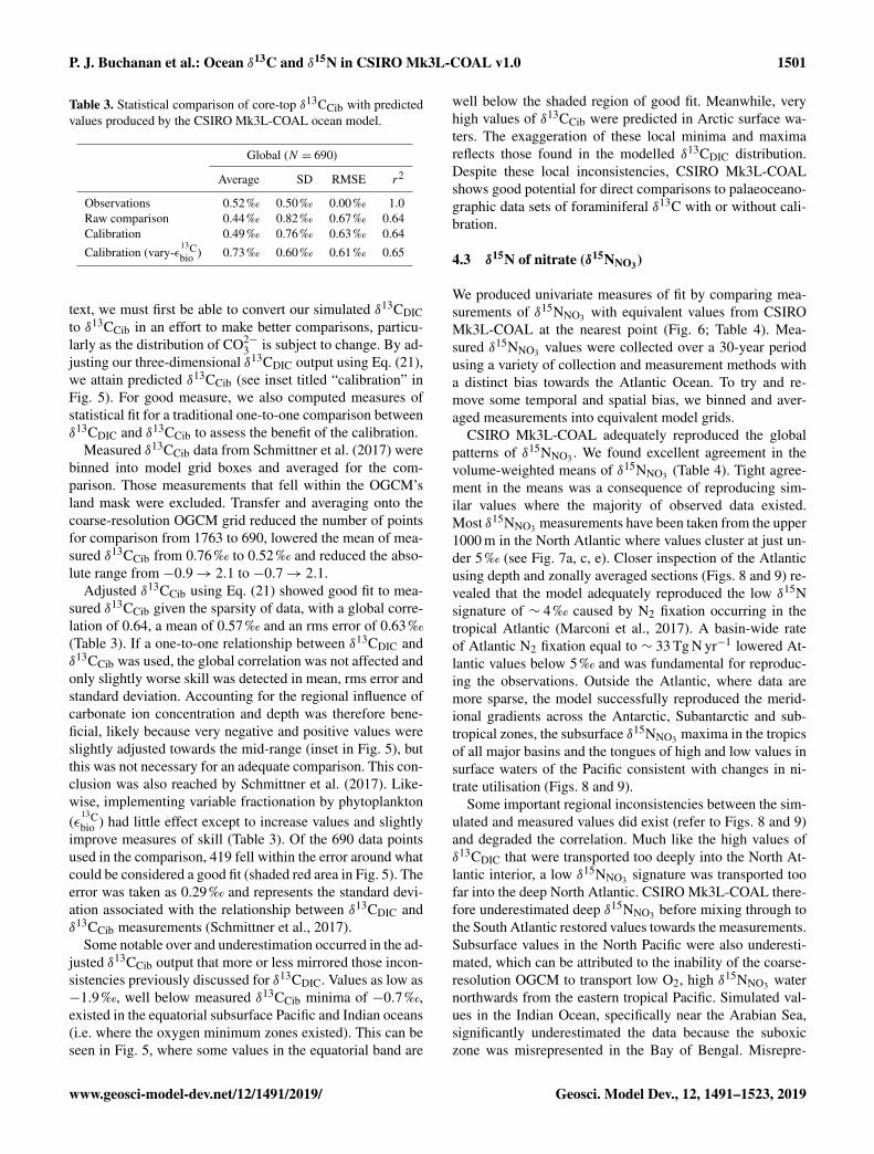
Table 3. Statistical comparison of core-top δ13CCib with predictedvalues produced by the CSIRO Mk3L-COAL ocean model.

Global (N = 690)

Average SD RMSE r2

Observations 0.52 ‰ 0.50 ‰ 0.00 ‰ 1.0Raw comparison 0.44 ‰ 0.82 ‰ 0.67 ‰ 0.64Calibration 0.49 ‰ 0.76 ‰ 0.63 ‰ 0.64Calibration (vary-ε

13Cbio ) 0.73 ‰ 0.60 ‰ 0.61 ‰ 0.65

text, we must first be able to convert our simulated δ13CDICto δ13CCib in an effort to make better comparisons, particu-larly as the distribution of CO2−

3 is subject to change. By ad-justing our three-dimensional δ13CDIC output using Eq. (21),we attain predicted δ13CCib (see inset titled “calibration” inFig. 5). For good measure, we also computed measures ofstatistical fit for a traditional one-to-one comparison betweenδ13CDIC and δ13CCib to assess the benefit of the calibration.

Measured δ13CCib data from Schmittner et al. (2017) werebinned into model grid boxes and averaged for the com-parison. Those measurements that fell within the OGCM’sland mask were excluded. Transfer and averaging onto thecoarse-resolution OGCM grid reduced the number of pointsfor comparison from 1763 to 690, lowered the mean of mea-sured δ13CCib from 0.76 ‰ to 0.52 ‰ and reduced the abso-lute range from −0.9→ 2.1 to −0.7→ 2.1.

Adjusted δ13CCib using Eq. (21) showed good fit to mea-sured δ13CCib given the sparsity of data, with a global corre-lation of 0.64, a mean of 0.57 ‰ and an rms error of 0.63 ‰(Table 3). If a one-to-one relationship between δ13CDIC andδ13CCib was used, the global correlation was not affected andonly slightly worse skill was detected in mean, rms error andstandard deviation. Accounting for the regional influence ofcarbonate ion concentration and depth was therefore bene-ficial, likely because very negative and positive values wereslightly adjusted towards the mid-range (inset in Fig. 5), butthis was not necessary for an adequate comparison. This con-clusion was also reached by Schmittner et al. (2017). Like-wise, implementing variable fractionation by phytoplankton(ε

13Cbio ) had little effect except to increase values and slightly

improve measures of skill (Table 3). Of the 690 data pointsused in the comparison, 419 fell within the error around whatcould be considered a good fit (shaded red area in Fig. 5). Theerror was taken as 0.29 ‰ and represents the standard devi-ation associated with the relationship between δ13CDIC andδ13CCib measurements (Schmittner et al., 2017).

Some notable over and underestimation occurred in the ad-justed δ13CCib output that more or less mirrored those incon-sistencies previously discussed for δ13CDIC. Values as low as−1.9 ‰, well below measured δ13CCib minima of −0.7 ‰,existed in the equatorial subsurface Pacific and Indian oceans(i.e. where the oxygen minimum zones existed). This can beseen in Fig. 5, where some values in the equatorial band are

well below the shaded region of good fit. Meanwhile, veryhigh values of δ13CCib were predicted in Arctic surface wa-ters. The exaggeration of these local minima and maximareflects those found in the modelled δ13CDIC distribution.Despite these local inconsistencies, CSIRO Mk3L-COALshows good potential for direct comparisons to palaeoceano-graphic data sets of foraminiferal δ13C with or without cali-bration.

4.3 δ15N of nitrate (δ15NNO3 )

We produced univariate measures of fit by comparing mea-surements of δ15NNO3 with equivalent values from CSIROMk3L-COAL at the nearest point (Fig. 6; Table 4). Mea-sured δ15NNO3 values were collected over a 30-year periodusing a variety of collection and measurement methods witha distinct bias towards the Atlantic Ocean. To try and re-move some temporal and spatial bias, we binned and aver-aged measurements into equivalent model grids.

CSIRO Mk3L-COAL adequately reproduced the globalpatterns of δ15NNO3 . We found excellent agreement in thevolume-weighted means of δ15NNO3 (Table 4). Tight agree-ment in the means was a consequence of reproducing sim-ilar values where the majority of observed data existed.Most δ15NNO3 measurements have been taken from the upper1000 m in the North Atlantic where values cluster at just un-der 5 ‰ (see Fig. 7a, c, e). Closer inspection of the Atlanticusing depth and zonally averaged sections (Figs. 8 and 9) re-vealed that the model adequately reproduced the low δ15Nsignature of ∼ 4 ‰ caused by N2 fixation occurring in thetropical Atlantic (Marconi et al., 2017). A basin-wide rateof Atlantic N2 fixation equal to ∼ 33 Tg N yr−1 lowered At-lantic values below 5 ‰ and was fundamental for reproduc-ing the observations. Outside the Atlantic, where data aremore sparse, the model successfully reproduced the merid-ional gradients across the Antarctic, Subantarctic and sub-tropical zones, the subsurface δ15NNO3 maxima in the tropicsof all major basins and the tongues of high and low values insurface waters of the Pacific consistent with changes in ni-trate utilisation (Figs. 8 and 9).

Some important regional inconsistencies between the sim-ulated and measured values did exist (refer to Figs. 8 and 9)and degraded the correlation. Much like the high values ofδ13CDIC that were transported too deeply into the North At-lantic interior, a low δ15NNO3 signature was transported toofar into the deep North Atlantic. CSIRO Mk3L-COAL there-fore underestimated deep δ15NNO3 before mixing through tothe South Atlantic restored values towards the measurements.Subsurface values in the North Pacific were also underesti-mated, which can be attributed to the inability of the coarse-resolution OGCM to transport low O2, high δ15NNO3 waternorthwards from the eastern tropical Pacific. Simulated val-ues in the Indian Ocean, specifically near the Arabian Sea,significantly underestimated the data because the suboxiczone was misrepresented in the Bay of Bengal. Misrepre-



Figure 5. Measured versus modelled δ13CCib (N = 690) of CSIRO Mk3L-COAL coloured by latitude. Red shading about the 1 : 1 line isan estimate of the variability implicit in the relationship between δ13CCib and δ13CDIC of Schmittner et al. (2017). The inset on the bottomright shows the effect of the calibration of Eq. (21).

Table 4. Comparison of global and region mean δ15NNO3 between observations and model simulations. Model means are annual averages.All data were regridded onto the CSIRO Mk3L-COAL grid space. The δ15N data (5330 measurements courtesy of the Sigman Lab, PrincetonUniversity) were binned into corresponding grid boxes and averaged for direct comparison, which reduced the data to 2532 points. Morethan one data point of δ15N may therefore contribute to each simulated value.

Global Southern Ocean Atlantic Pacific Indian

Data 5.4 ‰ 5.3 ‰ 4.8 ‰ 6.8 ‰ 6.7 ‰

CSIRO Mk3L-COAL 5.5 ‰ 5.4 ‰ 4.7 ‰ 7.8 ‰ 5.2 ‰UVic-MOBI 6.6 ‰ 5.5 ‰ 6.2 ‰ 7.6 ‰ 7.4 ‰PISCES 4.3 ‰ 4.6 ‰ 3.7 ‰ 5.6 ‰ 5.1 ‰iCESM-high 6.2 ‰ 5.3 ‰ 5.2 ‰ 8.6 ‰ 6.2 ‰

sentation of the northern Indian Ocean was responsible forvery poor model–data fit in the Indian Ocean (Fig. 6). Mean-while, the deep (> 1500 m) eastern tropical Pacific tended tooverestimate the data, due to a large, deep, unimodal suboxiczone. These physically driven inconsistencies in the oxy-gen field are common to other coarse-resolution models (Os-chlies et al., 2008; Schmittner et al., 2008) and, like the δ13Cdistribution, were the main cause of the misfit between simu-lated and observed δ15NNO3 . The correlations reflected theseregional under- and overestimations, particularly in the In-dian Ocean.

Finally, we placed CSIRO Mk3L-COAL in the context ofother isotope-enabled global models: UVic-MOBI, PISCESand iCESM-high (Table 1). This comparison demonstratedthat the modelled distribution of δ15NNO3 was adequatelyplaced among the current generation of models. The globaland regional means were more accurately reproduced byCSIRO Mk3L-COAL than for UVic-MOBI, PISCES andiCESM-high (Table 4; also see shading in Fig. 6). Atlanticδ15NNO3 was best reproduced by CSIRO Mk3L-COAL.Meanwhile, correlations tended to be slightly lower for

CSIRO Mk3L-COAL than UVic-MOBI and iCESM-high,and consistently lower than PISCES (Fig. 6). UVic-MOBIunderestimated the data but produced high correlations inthe Southern Ocean and globally. Regionally, PISCES wasbest correlated to the measurements of δ15NNO3 of the threemodels, although it had a consistent positive bias. iCESM-high was acceptably correlated with the data in the globalsense but was highest in rms errors, particularly in the Pacific.CSIRO Mk3L-COAL therefore showed an acceptable mea-sure of fit to the noisy and sparse δ15NNO3 data and repro-duced most regional patterns, albeit with misrepresentationin the Indian Ocean and some exaggerations of local min-ima/maxima as discussed. Future model–data comparisonswith CSIRO Mk3L-COAL should therefore take these limi-tations into account. Overall, however, we find that CSIROMk3L-COAL broadly reproduced the δ15NNO3 data. Annualrates of N2 fixation, water column denitrification and sedi-mentary denitrification at roughly 122, 52 and 78 Tg N yr−1,respectively, produced this agreement.

An important caveat to the δ15NNO3 routines of CSIROMk3L-COAL should be noted. CSIRO Mk3L-COAL under-



Figure 6. Global and regional fits between observations and simulated δ15NNO3 displayed as Taylor diagrams (Taylor, 2001). Shading ofthe markers represent normalised bias. G indicates global; S indicates Southern Ocean (90–40◦ S); A indicates Atlantic (40◦ S–70◦ N); Pindicates Pacific (40◦ S–70◦ N); I indicates Indian Ocean (40◦ S–70◦ N). The δ15N data (5330 measurements courtesy of the Sigman Lab,Princeton University) were binned into corresponding grid boxes and averaged for direct comparison, which reduced the data to 2532 points.More than one data point of δ15N may therefore contribute to each simulated value.

went significant tuning of water column and sedimentarydenitrification parameterisations in order to reproduce knownvalues of δ15NNO3 during development. One important pa-rameter is the lower threshold of NO3 concentration at whichpoint water column denitrification is shut off (Sect. A2.3).In CSIRO Mk3L-COAL, this is set at 30 mmol m−3, whichis an arbitrary limit that was implemented to prevent wa-ter column denitrification from reducing NO3 to zero in thelarge suboxic zones. Hence, a caveat of the current modelis an inability for water column and sedimentary denitrifi-cation to realistically adjust as suboxia changes. However,the parameterisation does allow for targeted experimentswhere the ratio of water column to sedimentary denitrifica-tion can be controlled if, for instance, it is unclear how wa-ter column and sedimentary denitrification respond to cer-tain conditions. This is currently the case during the LastGlacial Maximum, where expansive suboxic zones in the Pa-

cific (Hoogakker et al., 2018) were counter-intuitively as-sociated with reduced rates of water column denitrification(Ganeshram et al., 1995). We have, in this version, chosen tokeep this parameterisation and note that future developmentswill focus on dynamic responses to variations in suboxia.

4.4 δ15N of organic matter (δ15Norg)

CSIRO Mk3L-COAL tracks the δ15N signature of organicmatter (δ15Norg) that is deposited in the sediments. We com-pared the simulated δ15Norg to the core-top compilation ofTesdal et al. (2013) with 2176 records of δ15Norg. Theserecords were binned and averaged onto the CSIRO Mk3L-COAL ocean grid, such that the 2176 records became 592.When comparing sediment core-top measurements of δ15Nto that of the model, it is necessary to consider how δ15Norgis altered by early burial. As records in the compilation of



Figure 7. Observed (a, c, e) and modelled (b, d, f) δ15N of NO3 data (N = 5004) plotted against depth (a, b), latitude (c, d) and longitude (e,f). Colour shading represents the density of data, such that the darker a mass of data points is, the more data are represented there.

Figure 8. Depth-averaged sections of modelled (colour contours) and observed (overlaid markers) δ15NNO3 .

Tesdal et al. (2013) are from bulk nitrogen, we can assumethat the “diagenetic offset” as described by Robinson et al.(2012) is active. The diagenetic offset involves an increasein the δ15N of sedimentary nitrogen of between 0.5 ‰ and4.1 ‰ relative to that of sinking particulate organic matterand appears to be related to pressure (Robinson et al., 2012),although the reasoning behind this relationship remains to bedefined.

In light of the diagenetic offset, we make three compar-isons with the compilation of Tesdal et al. (2013). A raw

comparison is made, alongside an attempt to account for thediagenetic offset using two depth-dependent corrections (Ta-ble 5 and Fig. 10):

δ15Ncor:1org =

{δ15Norg, if z(km) < 1km

δ15Norg+(

1 · z(km)+ 1), if z(km)≥ 1km

(22)

δ15Ncor:2org = δ

15Norg+ 0.9 · z(km). (23)



Figure 9. Zonally averaged sections of modelled (colour contours) and observed (overlaid markers) δ15NNO3 . The global zonal averageencompasses all basins.

The first correction (δ15Ncor:1org ) is taken from Robinson

et al. (2012), while the second (δ15Ncor:2org ) originates from

how Schmittner and Somes (2016) treated sedimentary nitro-gen isotope data in their study of the Last Glacial Maximum.Both are based on the observation that the diagenetic offsetincreases with pressure, in this case represented by depth (z)in kilometres (km).

Following binning and averaging onto the model grid, theraw comparison immediately showed a consistent underesti-mation of the core-top data, with a predicted mean of 2.7 ‰well below the observed mean of 4.7 ‰. Our correlation was0.27, which indicates a limited ability to replicate regionalpatterns. This underestimation and low correlation is easilyseen when predicted values are compared directly to the core-top data in Fig. 10. Like the nitrogen isotope model of Someset al. (2010), we find that the offset between simulated andobserved core-top bulk δ15Norg is roughly equivalent to theobserved average diagenetic offset of∼ 2.3±1.8 ‰. This in-dicates that diagenetic alteration of δ15Norg is active duringearly burial in the core-top data.

Including a diagenetic offset therefore improved agree-ment between our predicted δ15Norg and the core-top dataconsiderably (Table 5 and Fig. 10). Both corrections ac-counted for the enrichment of δ15N in deeper regions andthe minor diagenetic alteration in areas of high sedimenta-tion that typically occurs in shallower sediments. The aver-age δ15Norg increased to 4.5 ‰ for δ15Ncor:1

org and 5.2 ‰ forδ15Ncor:2

org . Correlations increased from 0.27 to 0.47 and 0.53,respectively. The improvement was clearly observed in theSouthern Ocean, where both the magnitude and spatial pat-tern of δ15Norg were well replicated by the model. Changesin the Southern Ocean over glacial–interglacial cycles reflectshifts in the global marine nitrogen cycle and nutrient util-

isation (Martinez-Garcia et al., 2014; Studer et al., 2018),and the ability of CSIRO Mk3L-COAL to account for thesepatterns in the core-top data is encouraging for future study.We suggest that future palaeoceanographic model–data com-parisons of δ15Norg use the depth correction of Schmittnerand Somes (2016) as it provided the best correlations and re-produced Southern Ocean δ15Norg at 0.5 ‰ greater than theglobal mean (see Table 5).

5 Ecosystem effects

As a first test of the isotope-enabled ocean model, we under-took simple ecosystem experiments to assess the effect onδ13C and δ15N. For reference, the assessment of model per-formance described above used model output with variablestoichiometry activated, a fixed 8 % rain ratio of CaCO3 toorganic carbon and a strong iron limitation of N2 fixers thatenforced a low degree of spatial coupling between N2 fixersand denitrification zones. A summary of the biogeochemicaleffects of the different experiments is provided in Table 6.

5.1 Variable versus Redfieldian stoichiometry

Enabling variable stoichiometry (see Sect. A3 in the Ap-pendix) of the general phytoplankton group (PG

org) overa Redfieldian ratio (C : N : P : Orem

2 : NOrem3 = 106 : 16 : 1 :

−138 : −94.4) altered the rate and distribution of organicmatter export. Organic matter had more carbon and nitrogenper unit phosphorus in regions with low PO4, such as theAtlantic Ocean (Fig. 11a), which elevated O2 and NO3 de-mand during oxic and suboxic remineralisation (denitrifica-tion), respectively. Lower ratios were produced in eutrophicregions such as the subarctic Pacific, Southern Ocean and



Table 5. Statistical comparison of core-top δ15Norg with predicted values of the CSIRO Mk3L-COAL ocean model. The corrected vales(δ15Ncor:1

org and δ15Ncor:2org ) account for alteration during early diagenesis following burial.

Global (N = 592) Southern Ocean (N = 81)

Average SD r2 Average SD r2

Observations 4.7 ‰ 3.1 ‰ 1.0 5.2 ‰ 1.7 ‰ 1.0Raw comparison 2.7 ‰ 3.2 ‰ 0.27 1.1 ‰ 1.6 ‰ 0.13δ15Ncor:1

org 4.5 ‰ 3.8 ‰ 0.47 4.3 ‰ 1.8 ‰ 0.45δ15Ncor:2

org 5.2 ‰ 4.2 ‰ 0.53 5.7 ‰ 1.9 ‰ 0.47

Figure 10. Direct comparison of observed versus modelled δ15Norg incident on the sediments. Panels (a), (c) and (e) show spatial distributionof simulated δ15Norg overlain by core-top data from the compilation of Tesdal et al. (2013). Panels (b), (d) and (f) compare all core-top dataagainst simulated δ15Norg. Panels (a) and (b) depict raw output of the model, while panels (c)–(f) depict the predicted values of the modelfollowing two depth-dependent offsets (Eqs. 22 and 23) that account for diagenetic alteration.

tropical zones of upwelling. Overall, global mean C : P in-creased from the Redfieldian 106 : 1 to 117 : 1 and causedan increase in carbon export from 7.6 to 8.0 Pg C yr−1. Ap-proximately 0.1 Pg C yr−1, or 25 % of the increase, was at-tributed purely to organic carbon export from N2 fixation,which increased from 107 to 122 Tg N yr−1 as higher N : Pratios in the tropics broadened their competitive niche. Thetotal contribution of N2 fixation to the increase in carbon ex-

port was likely greater than 25 %, as NO3 also became moreavailable to NO3-limited ecosystems in the lower latitudes(Moore et al., 2013). The increase in carbon export undervariable stoichiometry as compared to a Redfieldian oceanwas therefore felt largely in the lower latitudes between 40◦ Sand 40◦ N (Fig. 11b). Export production decreased polewardof 40◦, particularly in the Southern Ocean, because C : P ra-tios were lower than the 106 : 1 Redfield ratio (Fig. 11a).



Table 6. Summary of the biogeochemical effects of the different treatments of the ecosystem in CSIRO Mk3L-COAL. Corg is the total organiccarbon exported from the euphotic zone composed of both general and diazotrophic phytoplankton groups (CG

org + CDorg; see Sect. A1 in the

Appendix), while CCaCO3 is the total export of CaCO3 out of the euphotic zone. The sum of Corg and CCaCO3 are equal to the global rateof carbon export referred to in the text. Sed : WC refers to the sedimentary to water column denitrification ratio. Note that the global meanδ13CDIC is higher than reported in Table 2 because it includes the upper 200 m and the Arctic.

Corg CCaCO3 N2 fix Sed : WC O2 Suboxia DIC δ13CDIC δ15NNO3

Pg C yr−1 Tg N yr−1 ratio mmol m−3 % ocean Pg C ‰

Variable versus Redfieldian stoichiometry (Sect. 5.1)

Redfield 7.08 0.52 107 1.5 187 1.5 33 908 0.47 5.1Variable 7.42 0.54 122 1.5 193 2.1 33 870 0.51 5.6

Calcifier dependence on calcite saturation state (Sect. 5.2)

Fixed (8 % of CGorg) 7.42 0.54 122 1.5 193 2.1 33 870 0.51 5.6

Variable (η = 0.53) 7.41 0.32 122 1.5 193 2.1 34 010 0.52 5.6Variable (η = 0.81) 7.41 0.47 122 1.5 193 2.1 33 916 0.50 5.6Variable (η = 1.09) 7.42 0.68 122 1.5 193 2.1 33 783 0.48 5.6

Strength of coupling between N2 fixation and denitrification (Sect. 5.3)

Weak 7.42 0.54 122 1.5 193 2.1 33 870 0.51 5.6Moderate 7.72 0.48 144 1.9 188 2.5 34 079 0.45 5.2Strong 7.59 0.46 154 2.1 187 2.7 34 182 0.42 5.0

Distributions of both isotopes were affected by the changein carbon export and the marine nitrogen cycle. Global meanδ13CDIC increased from 0.47 ‰ to 0.51 ‰ and δ15NNO3 in-creased from 5.1 ‰ to 5.6 ‰. These are not great changeson the global scale and they had little influence on model–data measures of fit. However, the spatial distribution of theseisotopes was significantly altered. Intermediate waters leav-ing the Southern Ocean were depleted in δ13CDIC by up to0.1 ‰ and δ15NNO3 by up to 1 ‰, while the deep ocean, par-ticularly the Pacific, was enriched in both isotopes to a sim-ilar degree (Fig. 12). Depletion of both isotopes in waterssubducted between 40 and 60◦ S reflected the local loss inexport production as a result of lower C : P and N : P ratios,such that biological fractionation was unable to enrich DICand NO3 in the heavier isotope to the same degree as surfacewaters travelled north. Enrichment of δ13C in the deep oceanwas the result of reduced carbon export in the Antarctic zonedue to low C : P ratios, while enrichment of δ15N in the deepocean was the result of increased tropical production that in-creased water column denitrification (ε

15Nwc = 20 ‰). Lower

C : P and N : P ratios in both the Antarctic and Subantarcticzones therefore elicited divergent isotope effects in deep andintermediate waters leaving the Southern Ocean.

Meanwhile, each isotope showed a different response inthe suboxic zones of the tropics where variable stoichiome-try increased the volume of suboxia (O2 < 10 mmol m−3) by0.5 %. The increase in water column denitrification causedby the expansion of suboxia increased δ15NNO3 , while the lo-cal increase in carbon export that drove the increase in watercolumn denitrification reduced δ13CDIC in the same waters

(Fig. 12). Overall, the increase in low-latitude carbon exportcaused an expansion of water column suboxia and eliciteddiverging behaviours in the isotopes, whereby δ15NNO3 in-creased and δ13CDIC decreased.

5.2 Calcifier dependence on calcite saturation state

The rate of calcification of planktonic foraminifera and coc-colithophores is dependent on the calcite saturation state(Zondervan et al., 2001). In previous experiments, the pro-duction of CaCO3 was fixed at a rate of 8 % per unitof organic carbon produced in accordance with the mod-elling study of Yamanaka and Tajika (1996) and produced0.54 Pg CaCO3 yr−1. Now we investigate how spatial vari-ations in the CaCO3 : Corg ratio (RCaCO3 in Eq. A17) af-fected δ13CDIC and δ13CCib (see Sect. A1.3 in the Appendix).We applied three different values of η to Eq. (A18) to alterthe quantity of CaCO3 produced per unit of organic carbon(CG

org) given the calcite saturation state (�ca). The η coeffi-cients were 0.53, 0.81 and 1.09. These numbers are equiva-lent to those in the experiments of Zhang and Cao (2016).

Mean RCaCO3 was 4.5 %, 6.6 % and 9.5 %, and annualCaCO3 production was 0.32, 0.47 and 0.68 Pg CaCO3 yr−1

in the three experiments. Although different in total CaCO3production, the three experiments shared the same spatialpatterns. Low-latitude waters were high in RCaCO3 , partic-ularly the oligotrophic subtropical gyres, while high lati-tudes were low, particularly the Antarctic zone where mix-ing of old waters into the surface depressed the calcite sat-uration state (Fig. 13). These regional patterns in RCaCO3



Figure 11. Simulated difference in the C : P ratio of exported organic matter due to variable stoichiometry as compared to Redfield stoi-chiometry (a) and the resulting change in carbon export out of the euphotic zone (b).

Figure 12. Differences in δ13CDIC (a) and δ15NNO3 (b) as a result of variable stoichiometry as compared to Redfield stoichiometry. Valuesare zonal means.



Figure 13. Global distribution of CaCO3 export as a percentage of organic carbon (Corg) export (a) and the change in the CaCO3 productionfield as a result of making CaCO3 production dependent on calcite saturation state (η = 1.09) compared to when it was a fixed 8 % ofCorg (b). Areas where export production does not occur due to severely nutrient limited conditions are masked out.

Figure 14. Changes in the distribution of carbon isotopes (δ13CDIC and δ13CCib; a) and carbon chemistry (dissolved inorganic carbon andalkalinity; b) as a result of increasing CaCO3 production in surface waters between 40◦ S and 40◦ N.



therefore had the largest effect in areas of high export pro-duction. Productive, high-latitude areas like the SouthernOcean, subpolar Pacific and North Atlantic waters all pro-duced less CaCO3 when compared to an enforced 8 % rainratio, while CaCO3 production between 40◦ S and 40◦ N rel-ative to a fixed RCaCO3 of 8 % was dependent on η. The high-est η coefficient of 1.09 achieved greater export of CaCO3 inthe mid- to lower-latitude regions of high export production(Fig. 13). The consequence of increasing CaCO3 productionin the middle–lower latitudes was a loss of upper ocean alka-linity, subsequent outgassing of CO2 and losses in the DICinventory. Losses in global DIC were 95 and 130 Pg C asRCaCO3 increased from 4.6→ 6.6→ 9.5 % (Table 6), equiv-alent to one-fifth of the glacial increase in oceanic carbon(Ciais et al., 2011).

Despite the significant changes associated with the im-plementation of �ca-dependent CaCO3 production, effectswere negligible on both δ13CDIC and δ13CCib. Global meanδ13CDIC was 0.51 ‰, when RCaCO3 was fixed at 8 %, andthis changed to 0.52 ‰, 0.50 ‰ and 0.48 ‰ under η coeffi-cients of 0.53, 0.81 and 1.09 (Table 6). Likewise, global meanδ13CCib was 0.59 ‰, when RCaCO3 was fixed at 8 %, and thischanged to 0.60 ‰, 0.58 ‰ and 0.55 ‰. Minimal change inδ13CCib indicated minimal change in the CO2−

3 concentra-tion (see Eq. 21), which varied by ≤ 2 mmol m−3 betweenexperiments. Visual inspection of the change in δ13CDIC andδ13CCib distributions showed an enrichment of these isotopesin the upper ocean north of 40◦ S. Subsequent increases inη, which increased low-latitude CaCO3 production, mag-nified the enrichment. Enrichment of δ13CDIC and δ13CCibwas caused by outgassing of CO2 as surface alkalinity de-creased in response to greater CaCO3 production (Fig. 14).The change, however, was at most 0.1 ‰, which lies wellwithin 1 standard deviation of variability known in the proxydata (Schmittner et al., 2017). We therefore find little scopefor recognising even large variations in global CaCO3 pro-duction (0.32 to 0.68 Pg CaCO3 yr−1) in the signature of car-bon isotopes despite considerable effects on the oceanic in-ventory of DIC.

However, we stress that version 1.0 of CSIRO Mk3L-COAL does not include CaCO3 burial or dissolution fromthe sediments according the calcite saturation state of over-lying water (Boudreau, 2013). To neglect ocean–sedimentCaCO3 cycling is to neglect of an important aspect of theglobal carbon cycle active on millennial timescales (Sigmanet al., 2010). Changes in CaCO3 burial and dissolution couldhave a non-negligible effect on δ13C through altering wholeocean alkalinity and thereby air–sea gas exchange of CO2,which would in turn affect surface δ13C as we have seen.While we do not address these effects here, we aim to doso in upcoming versions of the model equipped with carboncompensation dynamics.

Figure 15. Changes in the distribution of marine N2 fixation causedby altering how limiting iron is to the growth of N2 fixers via the co-efficient KDFe in Eq. (A12). Iron limitation is sequentially relaxedfrom top to bottom.

5.3 Strength of coupling between N2 fixation anddenitrification

The degree to which N2 fixers are spatially coupled to thetropical denitrification zones is controlled by altering thedegree to which N2 fixers are limited by iron (KDFe ) inEq. (A12) (see Sect. A1.2 in the Appendix). DecreasingKDFe

ensures that N2 fixation becomes less dependent on iron sup-ply and as such is released from regions of high aeolian de-position, such as the North Atlantic, to inhabit areas of lowNO3 : PO4 ratios. Areas of low NO3 : PO4 exist in the tropicsproximal to water column denitrification zones. Releasing N2fixers from Fe limitation therefore increases the spatial cou-pling between N2 fixation and water column denitrificationand increases the global rate of N2 fixation.

We steadily decreased iron limitation (KDFe ) to increasethe strength of spatial coupling between N2 fixers and thetropical denitrification zones (Fig. 15). As N2 fixers coupledmore strongly to regions of low NO3 : PO4, the rate of N2 fix-ation increased from 122 to 144 to 154 Tg N yr−1 (Table 6).An expansion of suboxia from 2.1 % to 2.5 % to 2.7 % ofglobal ocean volume in the tropics accompanied the increasein N2 fixation, as did a decrease in global mean δ13CDIC of0.06 ‰ and 0.1 ‰, since greater rates of N2 fixation stimu-



Figure 16. Change in δ15NNO3 caused by a stronger coupling between N2 fixation and tropical regions of low NO3 : PO4 concentrations(i.e. tropical upwelling zones with active water column denitrification). Panel (a) shows the global zonal mean change, while panel (b) showsthe average change in the euphotic zone, here defined as the top 100 m. Areas with very low NO3 (< 0.1 mmol m−3) are masked out.

lated tropical export production. Due to the expansion of thealready large suboxic zones, which occurred in both horizon-tal and vertical directions, the amount of organic carbon thatreached tropical sediments (20◦ S to 20◦ N) increased from0.35 to 0.46 to 0.51 Pg C yr−1.

The overarching consequence for δ15NNO3 due to an ex-pansion of the suboxic zones was an increase in the sedimen-tary to water column denitrification ratio from 1.5 to 1.9 to2.2, which decreased mean δ15NNO3 from 5.6 ‰ to 5.2 ‰to 5.0 ‰ (Table 6). The increase in N2 fixation (δ15Norg =

−1‰) and sedimentary denitrification (ε15Nsed = 3‰) in the

tropics was felt globally for δ15NNO3 (Fig. 16). Lowerδ15NNO3 by 0.5 ‰ and 0.9 ‰ permeated water columns inthe Southern Ocean and tropics, respectively. Meanwhile,δ15NNO3 was up to 10 ‰ lower in surface waters of thetropical and subtropical Pacific, which is where the greatestincrease in N2 fixation and sedimentary denitrification oc-curred. The dramatic reduction in surface δ15NNO3 was sub-sequently conveyed to the sediments as δ15Norg± 1 ‰–2 ‰.

These simple experiments demonstrate that the insightsgarnered from sedimentary records of δ15N are open tomultiple lines of interpretation. An expansion of the sub-oxic zones, normally associated with an increase in δ15NNO3

(Galbraith et al., 2013), could instead cause a decrease inδ15NNO3 if more organic matter reached the sediments tostimulate sedimentary denitrification. There is good evidence

that the suboxic zones might have undergone a vertical ex-pansion (Hoogakker et al., 2018) and that more organic mat-ter reached the tropical sediments under glacial conditions(Cartapanis et al., 2016). The glacial decrease in bulk δ15Norgrecorded in the eastern tropical Pacific (Ganeshram et al.,1995; Liu et al., 2008) therefore does not necessarily meana decrease in suboxia. Rather, our experiments show thatlower δ15Norg might also be caused by an increase in lo-cal N2 fixation and sedimentary denitrification. The decreasein δ15NNO3 associated with more sedimentary denitrificationand local N2 fixation demonstrates the complexity of inter-preting sedimentary δ15Norg records in the lower latitudes.

6 Conclusions

The stable isotopes of carbon (δ13C) and nitrogen (δ15N) areproxies that have been fundamental for understanding theocean. We have included both isotopes into the ocean compo-nent of an Earth system model, CSIRO Mk3L-COAL, to en-able future studies with the capability for direct model–proxydata comparisons. We detailed how these isotopes are simu-lated, how to conduct model–data comparisons using bothwater column and sedimentary data and some basic assess-ment of changes caused by altered ecosystem functioning.We made three overall findings. First, CSIRO Mk3L-COALperforms well alongside a number of isotope-enabled global



ocean GCMs. Second, alteration of δ13C during formationof foraminiferal calcite does not jeopardise simple one-to-one comparisons with simulated δ13C of DIC, while diage-netic alteration of bulk organic δ15N during early burial mustbe accounted for in model–data comparisons. Third, changesin how marine ecosystems function can have significant andcomplex effects on δ13C and δ15N. Our idealised experi-ments hence showed that the interpretation of palaeoceano-graphic records may suffer from multiple lines of interpreta-tion, particularly records from the lower latitudes where mul-tiple processes imprint on the isotopic signatures laid downin sediments. Future work will involve palaeoceanographicsimulations of CSIRO Mk3L-COAL that seek to understandhow the oceanic carbon and nitrogen cycles respond to andinfluence important climate transitions.

Data availability. All model output is provided for down-load on Australia’s National Computing Infrastructure (NCI)at https://geonetwork.nci.org.au/geonetwork/srv/eng/catalog.search\T1\textbackslash#/metadata/f3048_7378_3224_4737(last access: 12 April 2019) and is citable withhttps://doi.org/10.25914/5c6643f64446c (Buchanan et al.,2019). Nitrogen isotope data are available by request to DarioM. Marconi and Daniel M. Sigman at Princeton Univer-sity. LOVECLIM data are freely available for download athttps://doi.org/10.4225/41/58192cb8bff06 (Menviel et al., 2017b).UVic-MOBI data were provided by Christopher Somes, PISCESdata by Laurent Bopp, iCESM-high data from Simon Yang andiCESM-low data by Alexandra Jahn.

Code availability. The source code for CSIRO Mk3L-COAL is shared via a repository located at http://svn.tpac.org.au/repos/CSIRO_Mk3L/branches/CSIRO_Mk3L-COAL/(last access: 12 April 2019). Access to the reposi-tory may be obtained by following the instructions athttps://www.tpac.org.au/csiro-mk3l-access-request/ (last ac-cess: 12 April 2019). Access to the source code is subject to abespoke license that does not permit commercial usage but isotherwise unrestricted. An “out-of-the-box” run directory is alsoavailable for download with all files required to run the model inthe configuration used in this study, although users will need tomodify the runscript according to their computing infrastructure.


https://geonetwork.nci.org.au/geonetwork/srv/eng/catalog.search#/metadata/f3048_7378_3224_4737

https://geonetwork.nci.org.au/geonetwork/srv/eng/catalog.search#/metadata/f3048_7378_3224_4737

https://doi.org/10.25914/5c6643f64446c

https://doi.org/10.4225/41/58192cb8bff06

http://svn.tpac.org.au/repos/CSIRO_Mk3L/branches/CSIRO_Mk3L-COAL/

http://svn.tpac.org.au/repos/CSIRO_Mk3L/branches/CSIRO_Mk3L-COAL/

https://www.tpac.org.au/csiro-mk3l-access-request/


Appendix A: Ecosystem component of the OBGCM

A1 Export production

A1.1 General phytoplankton group (G)

The production of organic matter by the general phytoplank-ton group (PG

org) is measured in units of mmol phosphorus(P) m−3 d−1 and is dependent on temperature (T ), nutrients(PO4, NO3 and Fe) and irradiance (I ):

PGorg = SG

E:P ·µ(T )G·min

(PG

lim,NGlim,FeG

lim,F (I )), (A1)

where

SGE:P = 0.005 mmolPO4 m3

µ(T )G = 0.59 · 1.0635T (A2)

F(I)= 1− eL(I) (A3)

L(I)=I ·α ·PARµ(T )

. (A4)

In the example above, SE:P converts growth rates in unitsof d−1 to mmol PO4 m−3 d−1. SE:P conceptually representsthe export to production ratio, and for simplicity we assumeit does not change. µ(T ) is the temperature-dependent maxi-mum daily growth rate of phytoplankton (doubling per day),as defined by Eppley (1972). The light limitation term (F(I))is the productivity versus irradiance equation used to de-scribe phytoplankton growth defined by Clementson et al.(1998) and is dependent on I , the daily averaged shortwaveincident radiation (W m−2), α, the initial slope of the pro-ductivity versus radiance curve (d−1 (W m−2)−1) and PAR,the fraction of shortwave radiation that is photosyntheticallyactive.

The nutrient limitation terms (PGlim, NG

lim and FeGlim) may be

calculated in two ways.If the option for static nutrient limitation is true, then

Michaelis–Menten kinetics (Dugdale, 1967) is used:

PGlim =

PO4

PO4+KGPO4

(A5)

NGlim =

NO3

NO3+KGNO3

(A6)

FeGlim =

FeFe+KG

Fe. (A7)

Half-saturation coefficients (KGnutrient ) show a large rangeacross phytoplankton species (e.g. Timmermans et al., 2004),and so for simplicity, we set KGPO4 = 0.1 mmol PO4 m−3

(Smith, 1982), KGNO3 = 0.75 mmol NO3 m−3 (Epp-ley et al., 1969; Carpenter and Guillard, 1971) andKGFe = 0.1 µmol Fe m−3 (Timmermans et al., 2001).

If the option for variable nutrient limitation is true (de-fault), then optimal uptake kinetics (Smith et al., 2009) is

used:

PGlim = PO4 /

( PO4

1− fA+

V/A

fA ·N : P

)(A8)

NGlim = NO3 /

( NO3

1− fA+V/A

fA

)(A9)

FeGlim =

FeFe+KFe

, (A10)

where

fA =max[(

1+

√[NO3]

V/A

)−1

,

(1+

√[PO4] ·N : P

V/A

)−1]. (A11)

Optimal uptake kinetics varies the two terms in the denom-inator of the Michaelis–Menten form according to the avail-ability of nutrients. It therefore accounts for different phy-toplankton communities with different abilities for nutrientuptake and does so using the fA term. The V/A term rep-resents the maximum potential nutrient uptake, V , over thecellular affinity for that nutrient, A, and is set at 0.1.

A1.2 Diazotrophs (D; N2 fixers)

Organic matter produced by diazotrophs (PDorg) is also mea-

sured in units of mmol phosphorus (P) m−3 d−1 and is calcu-lated in the same form of Eq. (A1), but using the maximumgrowth rate µ(T )D of Kriest and Oschlies (2015), notablechanges in the limitation terms and minimum thresholds thatensure the nitrogen fixation occurs everywhere in the ocean,except under sea ice. PD

org is calculated via

PDorg = SD

E:P ·µ(T )D·max

(0.01, min

(ND

lim,Plim,FeDlim))

·(1− ico

), (A12)

whereµ(T )D =max

(0.01, −0.0042T 2

+ 0.2253T − 2.7819)

(A13)

NDlim = e

−NO3 (A14)

PDlim =

PO4

PO4+KDPO4

(A15)

FeDlim =max

(0.0, tanh

(2Fe−KDFe)

). (A16)

The half-saturation values for PO4 and Fe limitation are setat 0.1 mmol m−1 and 0.5 µmolm−1, respectively, in the de-fault parameterisation. The motivation for making N2 fixersstrongly limited by Fe was the high cellular requirements ofFe for diazotrophy (see Sohm et al., 2011, and referencestherein). A dependency on light is omitted from the limita-tion term when PD

org is produced. The omission of light isjustified by its strong correlation with sea surface tempera-ture (Luo et al., 2014) and its negligible effect on nitrogenfixation in the Atlantic Ocean (McGillicuddy, 2014). Finally,



the fractional area coverage of sea ice (ico) is included to en-sure that cold water N2 fixation (Sipler et al., 2017) does notoccur under ice, since a light dependency is omitted.

A1.3 Calcifiers

The calcifying group produces calcium carbonate (CaCO3)in units of mmol carbon (C) m−3 d−1. The production ofCaCO3 is always a proportion of the organic carbon exportof the general phytoplankton group (CG

org), according to

CaCO3 = CGorg ·RCaCO3 . (A17)

The ratio of CaCO3 to CGorg (RCaCO3 ) can be calculated in

two ways.If the option for fixedRCaCO3 is true (default), thenRCaCO3

is set to 0.08 as informed by the experiments of Yamanakaand Tajika (1996). The production of CaCO3 is thus 8 % ofCG

org everywhere.If the option for variable RCaCO3 is true, then RCaCO3

varies as a function of the saturation state of calcite (�ca)according to Ridgwell et al. (2007), where

RCaCO3 = 0.022 ·(�ca− 1

)η. (A18)

The exponent (η) is easily modified consistent with the pa-rameterisations of Zhang and Cao (2016) and controls therate of CaCO3 production at a given value of �ca.

A2 Remineralisation


Organic matter produced by the general phytoplankton group(in units of phosphorus: PG

org) at the surface is instantaneouslyremineralised each time step at depth levels beneath the eu-photic zone using a power law scaled to depth (Martin et al.,1987). This power law defines the concentration of organicmatter remaining at a given depth (PG,z

org ) as a function of or-ganic matter at the surface (PG,0

org ) and depth itself (z). Its formis as follows:

PG,zorg = PG,0

org ·( z

zrem

)b, (A19)

where zrem in the denominator represents the depth at whichremineralisation begins and is set to be 100 m everywhere.The OBGCM therefore does not consider sinking speeds oran interaction between organic matter and physical mixing.However, variations in the b exponent affect the steepness ofthe curve, thereby emulating sinking speeds and affecting thetransfer and release of nutrients from the surface to the deepocean.

Remineralisation of PGorg through the water column is

therefore dependent on the exponent b value in Eq. (A19).The b exponent is calculated in two ways.

If the option for static remineralisation is true, then b is setto −0.858 according to Martin et al. (1987).

If the option for variable remineralisation is true (default),then b is dependent on the component fraction of picoplank-ton (Fpico) in the ecosystem. The Fpico shows a strong in-verse relationship to the transfer efficiency (Teff) of organicmatter from beneath the euphotic zone to 1000 m depth (We-ber et al., 2016). Because Fpico is not explicitly simulated inOBGCM, we estimate Fpico from the export production fieldin units of carbon (CG

org), calculate Teff using the parameteri-sation of Weber et al. (2016) and subsequently calculate theb exponent:

Fpico = 0.51− 0.26 ·CG

org (mgCm−2 h−1)

CG,maxorg (mgCm−2 h−1)

(A20)

Teff = 0.47− 0.81 ·Fpico (A21)

b =log(Teff)

log( 1000100 )= log(Teff). (A22)

A2.2 Diazotrophs (D)

Remineralisation of diazotrophs (PDorg) is calculated in the

same way as the general phytoplankton group (PGorg), with

the exception that the depth at which remineralisation occursis raised from 100 to 25 m in Eq. (A19). This alteration em-ulates the release of NO3 from N2 fixers well within the eu-photic zone, which in some cases can exceed the physicalsupply from below (Capone et al., 2005). Release of theirN- and C-rich organic matter (see stoichiometry Sect. A3.2)therefore occurs higher in the water column than the generalphytoplankton group.

A2.3 Suboxic environments

The remineralisation of PGorg and PD

org will typically requireO2 to be removed, except for in regions where oxygen con-centrations are less than a particular threshold (DenO2lim ),which is set to 7.5 mmol O2 m−3 and represents the onsetof suboxia. In these regions, the remineralisation of organicmatter begins to consume NO3 via the process of denitrifica-tion. We calculate the fraction of organic matter that is rem-ineralised by denitrification (Fden) via

Fden =(

1− e−0.5·DenO2lim + eO2−0.5·Den

O2lim

)−1, (A23)

such that Fden rises and plateaus at 100 % in a sigmoidalfunction as O2 is depleted from 7.5 to 0 mmol m−3.

Following this, the strength of denitrification is reducedif the ambient concentration of NO3 is deemed to be lim-iting. Denitrification within the modern oxygen minimumzones only depletes NO3 towards concentrations between15 and 40 mmol m−3 (Codispoti and Richards, 1976; Vosset al., 2001). Without an additional constraint that weakensdenitrification as NO3 is drawn down, here defined as rden,



NO3 concentrations quickly go to zero in simulated sub-oxic zones (Schmittner et al., 2008). We weaken denitrifi-cation by prescribing a lower bound at which NO3 can nolonger be consumed via denitrification, DenNO3

lim , which is setat 30 mmol NO3 m−3.

rden = 0.5+ 0.5 · tanh(

0.25 ·NO3− 0.25 ·DenNO3lim − 2.5)

(A24)if Fden > rden, then Fden = rden (A25)

Fden is therefore reduced if NO3 is deemed to be limitingand subsequently applied against both PG

org and PDorg to get

the proportion of organic matter to be remineralised by O2and NO3.

If the availability of O2 and NO3 is insufficient to reminer-alise all the organic matter at a given depth level, z, then theunremineralised organic matter will pass into the next depthlevel. Unremineralised organic matter will continue to passinto lower depth levels until the final depth level is reached, atwhich point all organic matter is remineralised by either wa-ter column or sedimentary processes. This version of CSIROMk3L-COAL does not consider burial of organic matter.

A2.4 Calcifiers

The dissolution of CaCO3 is calculated using an e-foldingdepth-dependent decay, where the amount of CaCO3 at agiven depth z is defined by

CaCO3z= CaCO3

0· e−zzdis , (A26)

where zdis represents the depth at which e−1 of CaCO3 (∼0.37) produced at the surface remains undissolved.

Calcifiers are not susceptible to oxygen-limited remineral-isation or the concentration of carbonate ion because the dis-solution of CaCO3 depends solely on this depth-dependentdecay. All CaCO3 reaching the final depth level is reminer-alised without considering burial. Future work will include afull representation of carbonate compensation.

A3 Stoichiometry

The elemental constitution, or stoichiometry, of organic mat-ter affects the biogeochemistry of the water column throughuptake (production) and release (remineralisation). The gen-eral phytoplankton group and diazotrophs both affect carbonchemistry, O2 and nutrients (PO4, NO3 and Fe), while thecalcifiers only affect carbon chemistry tracers (DIC, DI13Cand ALK).

Alkalinity ratios for both the general and nitrogen-fixinggroups are the negative of the N : P ratio, such that for a lossof 1 mmol of NO3, alkalinity will increase at 1 mmol eq m−3

(Wolf-Gladrow et al., 2007).


The stoichiometry of the general phytoplankton group is cal-culated in two ways.

If the option for static stoichiometry is true, then the C :N : Fe : P ratio is set according to the Redfield ratio of 106 :16 : 0.00032 : 1 (Redfield et al., 1937).

If the option for variable stoichiometry is true (default),then the C : N : P ratio of PG

org is made dependent on the am-bient nutrient concentration according to Galbraith and Mar-tiny (2015):

C : P=(6.9 · [PO4] + 6

1000

)−1(A27)

N : C= 0.125+0.03 · [NO3]

0.32+ [NO3](A28)

N : P= C : P ·N : C. (A29)

Thus, the stoichiometry of PGorg varies across the ocean ac-

cording to the nutrient concentration, and the uptake and re-lease of carbon, nutrients and oxygen (see Sect. A3.4) are de-pendent on the concentration of surface PO4 and NO3. Theratio of iron to phosphorus (Fe : P) remains fixed at 0.00032,such that 0.32 µmol of Fe is consumed per mmol of PO4.We chose to maintain a fixed Fe : P ratio because phyto-plankton communities from subtropical to Antarctic watersappear to show similar iron content (Boyd et al., 2015), de-spite changes in C : N : P. However, the ratio of C : N : Fedoes change as a result of varying C : N : P ratios, with higherC : Fe in oligotrophic environments and lower C : Fe in eu-trophic regions.

A3.2 Diazotrophs (D)

The stoichiometry of diazotrophs is fixed at a C : N : P : Feratio of 331 : 50 : 1 : 0.00064, which represents values re-ported in the literature (Kustka et al., 2003; Karl and Letelier,2008; Mills and Arrigo, 2010). Diazotrophs do not consumeNO3; rather, they consume N2, which is assumed to be ofunlimited supply, and release NO3 during remineralisation.

A3.3 Calcifiers

Calcifying organisms produce CaCO3, which includes DIC,DI13C and ALK, and these tracers are consumed and releasedat a ratio of 1 : 0.998 : 2, respectively, relative to organic car-bon. Thus, the ratio of C : DI13C : ALK relative to each unitof phosphorus consumed by the general phytoplankton groupis equal to the rain ratio of CaCO3 to organic phosphorusmultiplied by 106 : 105.8 : 212. This group has no effect onnutrient tracers or oxygen values.

A3.4 Stoichiometry of remineralisation

The requirements for oxygen (Orem2 : P) and nitrate (NOrem

3 :

P) during oxic and suboxic remineralisation, respectively, arecalculated from the C : N : P ratios of organic matter via theequations of Paulmier et al. (2009). Additional knowledgeof the hydrogen and oxygen content of the organic matter isalso required to calculate Orem

2 : P and NOrem3 : P. However,



the hydrogen and oxygen content of phytoplankton dependsstrongly on the proportions of lipids, carbohydrates and pro-teins that constitute the cell. As there is no empirical modelfor predicting these physiological components based on en-vironmental variables, we continue Redfield’s legacy by as-suming that all organic matter is a carbohydrate of the formCH2O. Future work, however, should address this obviousbias.

To calculate Orem2 : P and NOrem

3 : P, we therefore need tofirst calculate the amount of hydrogen and oxygen in organicmatter via

H : P= 2C : P+ 3N : P+ 3 (A30)O : P= C : P+ 4. (A31)

Once a C : N : P : H : O ratio for organic matter is known, wecalculate Orem

2 : P and NOrem3 : P in units of mmol m−3 P−1

using the equations of Paulmier et al. (2009):

Orem2 : P= − (C : P+ 0.25H : P− 0.5O : P− 0.75N : P

+ 1.25)− 2N : P (A32)NOrem

3 : P=− (0.8C : P+ 0.25H : P− 0.5O : P− 0.75N : P+ 1.25)+ 0.6N : P. (A33)

The calculation of Orem2 : P accounts for the oxygen that is

also needed to oxidise ammonium to nitrate.From these calculations, we find the following require-

ments of oxic and suboxic remineralisation, assuming thestatic stoichiometry option for the general phytoplanktongroup:

Orem2 : PG

org = 138

NOrem3 : PG

org = 94.4

O2rem : PDorg = 431

NOrem3 : PD

org = 294.8.

These numbers change dynamically alongside C : N : P ra-tios when the stoichiometry of organic matter is allowed tovary.

A4 Sedimentary processes

The remineralisation of organic matter within the sedimentsis provided as an option in the OBGCM. Sedimentary deni-trification, and its slight preference for the light isotopes offixed nitrogen (ε

15Nsed = 3 ‰), is an important component of

the marine nitrogen cycle and its isotopes. It acts as an addi-tional sink of NO3 and reduces the δ15N value of the globalocean by offsetting the strong fractionation of water columndenitrification (ε

15Nwc = 20 ‰).

If sedimentary processes are active, the empirical modelof Bohlen et al. (2012) is used to estimate the rate of sedi-mentary denitrification, where the removal of NO3 is depen-dent on the rate of particulate organic carbon (CG

org + CDorg)

arriving at the sediments and the ambient concentrations ofoxygen and nitrate. In the following, we assume that the con-centrations of NO3 and O2 that are available in the sedimentsare two-thirds of the concentration in the overlying water col-umn based on observations of transport across the diffusiveboundary layer (Gundersen and Jorgensen, 1990).

1NO3(sed)=(α+β · 0.98

(O2−NO3

))·

(CG

org+CDorg

)(A34)

where α = 0.04 and β = 0.1 (A35)

In the example above, both the α and β values were halvedfrom the values of Bohlen et al. (2012) to raise global meanNO3 concentrations and lower the sedimentary to water col-umn denitrification ratio to between 1 and 2. If NO3 is notavailable, the remaining organic matter is remineralised us-ing oxygen if the environment is sufficiently oxygenated. Anadditional limitation is set for sediments underlying hypoxicwaters (O2 < 40 mmol m−3), where oxic remineralisation isweakened towards zero according to a hyperbolic tangentfunction (0.5+0.5·tanh(0.2·O2−5)). If oxygen is also limit-ing, the remaining organic matter is remineralised via sulfatereduction. As sulfate is not explicitly simulated, we assumedthat sulfate is always available to account for the remainingorganic matter.

Thus, sedimentary denitrification is heavily dependent onthe rate of organic matter arriving at the sediments. However,a large amount of sedimentary remineralisation is not cap-tured using only these parameterisations because the coarseresolution of the OGCM enables it to resolve only the largestcontinental shelves, such as the shallow Indonesian seas.Many small areas of raised bathymetry in pelagic environ-ments are also unresolved by the OGCM. To address thisinsufficiency and increase the global rate of sedimentationand sedimentary denitrification, we coupled a subgrid-scalebathymetry to the coarse-resolution OGCM following themethodology of Somes et al. (2013) using the Earth topog-raphy 5 min grid (ETOPO5) 1/12◦ dataset. For each latitude-by-longitude grid point, we calculated the fraction of areathat would be represented by shallower levels in the OGCMif this finer-resolution bathymetry were used. At each depthlevel above the deepest level, the fractional area representedby sediments on the subgrid-scale bathymetry can be usedto remineralise all forms of exported matter (CG

org, CDorg and

CaCO3) via sedimentary processes.Also following the methodology of Somes et al. (2013),

we included an option to amplify sedimentary denitrifica-tion in the upper 250 m to account for narrow continentalshelves that are not resolved by the OGCM. Narrow shelvesexperience strong rates of upwelling and productivity, andhence high rates of sedimentary denitrification (Gruber andSarmiento, 1997). To amplify shallow rates of sedimentarydenitrification, we included an optional acceleration factor(0sed), set to 3.0 in the default parameterisation, dependenton the total fraction of shallower depths not covered by the



subgrid-scale bathymetry:

1NO3(sed)=1NO3(sed) ·((

1−Fsgb)·0sed+ 1

). (A36)

For those grids with a low fraction covered by the subgrid-scale bathymetry (Fsgb), the amplification of sedimentarydenitrification is therefore greatest.

Appendix B: Parameterisation of the OBGCMecosystem component

Default parameters for the marine ecosystem component ofCSIRO Mk3L-COAL are outlined in Tables B1, B2 and B3.The values presented in these tables are required as inputwhen running the ocean model.

Table B1. Parameter values controlling export production in the ecosystem component of the CSIRO Mk3L-COAL ocean model. Defaultsettings: Michaelis–Menten == False, Optimal Uptake == True, fix == True and Vary CaCO3 == False.

Parameter Action Value Active when

General phytoplankton (G)

SGE:P Export-to-production ratio 0.005 mmol P m−3 d−1 Always

α Initial slope of production versus irradiance curve 0.025 d−1 (W m−2)−1 AlwaysPAR Fraction of shortwave radiation that is photosynthetically active 0.5 AlwaysK

GPO4 Half-saturation coefficient for phosphate 0.1 mmol P m−3 Michaelis–Menten == TrueK

GNO3 Half-saturation coefficient for nitrate 0.75 mmol N m−3 Michaelis–Menten == TrueKGFe Half-saturation coefficient for iron 0.1 µmolFem−3 Michaelis–Menten == TrueV/A Maximum potential uptake over affinity for nutrient 0.1 Optimal Uptake == True

Diazotrophs (D)

SDE:P Export-to-production ratio 0.005 mmol P m−3 d−1 fix == True

KDFe Half-saturation coefficient for iron 0.5 µmolFem−3 fix == TrueKDFe Half-saturation coefficient for phosphate 0.1 mmol PO4 m−3 fix == True

Calcifiers

RCaCO3 Ratio of CaCO3 produced per unit carbon of PGorg 0.08 Vary CaCO3 == False

RCaCO3 Ratio of CaCO3 produced per unit carbon of PGorg 0.022 Vary CaCO3 == True

η Exponent varying RCaCO3 due to calcite saturation 0.53, 0.81 or 1.09 Vary CaCO3 == True



Table B2. Parameter values controlling remineralisation in the ecosystem component of the CSIRO Mk3L-COAL ocean model. Defaultsettings: ReminPico == True, fix == True, den == True and sedfluxes == True.



b Remineralisation profile exponent −0.858 ReminPico == Falseb Remineralisation profile exponent −0.7 to −1.2 ReminPico == Truezrem Depth at which remineralisation begins 100 m Always

Diazotrophs (D)

zrem Depth at which remineralisation begins 25 m fix == True

Calcifiers

zdis Depth at which e−1 CaCO3 remains undissolved 3500 m Always

Suboxic environments (affects G and D)

DenO2lim Dissolved oxygen concentration when denitrification begins 7.5 mmol m−3 den == True

DenO2lim Nitrate concentration when denitrification is limited 30.0 mmol m−3 den == True

Sediments (affects G and D)

α First constant in Bohlen Eq. (A34) 0.04 sedfluxes == Trueβ Second constant in Bohlen Eq. (A34) 0.1 sedfluxes == True0sed Sedimentary remineralisation amplification factor 3.0 sedfluxes == True

Table B3. Parameter values controlling stoichiometry in the ecosystem component of the CSIRO Mk3L-COAL ocean model. Default settings:Vary Stoich == True, Vary frac13 == False and fix == True.



C : ALK : N : Fe : P Nutrient stoichiometry of general phytoplankton 106 : −16 : 16 : 0.00032 : 1 Vary Stoich == FalseOrem

2 : NOrem3 : P Remineralisation requirements of O2 and NO3 −138 : −94.4 : 1 Vary Stoich == False

C : P Carbon stoichiometry of general phytoplankton (50 to 170) : 1 Vary Stoich == TrueN : P Nitrogen stoichiometry of general phytoplankton (7 to 26) : 1 Vary Stoich == TrueOrem

2 : P Remineralisation requirements of O2 (−220 to − 60) : 1 Vary Stoich == TrueNOrem

3 : P Remineralisation requirements of NO3 (−42 to − 150) : 1 Vary Stoich == True

ε13Cbio Carbon isotope fractionation during biological assimilation 21 ‰ Vary frac13 == False

ε13Cbio Carbon isotope fractionation during biological assimilation 15 ‰ to 25 ‰ Vary frac13 == True

Diazotrophs (D)

C:13C : ALK : N : Fe : P Nutrient stoichiometry of general phytoplankton 331 : 327 : −50 : 50 : 0.00064 : 1 fix == TrueOrem

2 : NOrem3 : P Remineralisation requirements of O2 and NO3 −431 : −294.8 : 1 fix == True

Calcifiers

C:13C : ALK : P Nutrient stoichiometry of calcifiers 106 : 105.8 : 212 : 1 Always



Supplement. The supplement related to this article is availableonline at: https://doi.org/10.5194/gmd-12-1491-2019-supplement.

Author contributions. PJB designed the study, undertook model de-velopment, ran the experiments, analysed model output and wrotethe manuscript. RJM designed the study, provided instruction ondevelopment, aided in analysis and edited the manuscript. ZC de-signed the study, aided in analysis and edited the manuscript. SJPaided in model development and edited the manuscript. NLB aidedin interpretation of results and edited the manuscript.

Competing interests. The authors declare that there is no conflict ofinterest.

Acknowledgements. The Australian Research Council’s Centre ofExcellence for Climate System Science and the Tasmanian Part-nership for Advanced Computing (TPAC) were instrumental forthis research. This research was supported under the AustralianResearch Council’s Special Research Initiative for the AntarcticGateway Partnership (project ID SR140300001). The authors wishto acknowledge the use of the Ferret programme for the analy-sis undertaken in this work. Ferret is a product of NOAA’s Pa-cific Marine Environmental Laboratory (information is availableat http://ferret.pmel.noaa.gov/Ferret/, last access: 12 April 2019).The Matplotlib package (Hunter, 2007) and the cmocean package(Thyng et al., 2016) were used for producing the figures. We are in-debted to Kristen Karsh, Daniel Sigman, Dario Marconi and EricRaes for discussions that focussed this work. Special thanks aregiven to Christopher Somes for correspondence in some develop-ment steps and revisions that improved the manuscript. Finally,the lead author is indebted to an Australian Fulbright postgradu-ate scholarship, which supported him at the Princeton Geosciencesdepartment during the writing of the manuscript.

Review statement. This paper was edited by Andrew Yool and re-viewed by Christopher Somes and two anonymous referees.

References

Altabet, M. A. and Francois, R.: Nitrogen isotope biogeochemistryof the Antarctic Polar Frontal Zone at 170 degrees W, Deep-Sea Res. Pt. II, 48, 4247–4273, https://doi.org/10.1016/S0967-0645(01)00088-1, 2001.

Bohlen, L., Dale, A. W., and Wallmann, K.: Simple trans-fer functions for calculating benthic fixed nitrogen lossesand C : N : P regeneration ratios in global biogeochem-ical models, Global Biogeochem. Cy., 26, GB3029,https://doi.org/10.1029/2011GB004198, 2012.

Boudreau, B. P.: Carbonate dissolution rates at thedeep ocean floor, Geophys. Res. Lett., 40, 744–748,https://doi.org/10.1029/2012GL054231, 2013.

Boyd, P. W., Strzepek, R. F., Ellwood, M. J., Hutchins, D. A.,Nodder, S. D., Twining, B. S., and Wilhelm, S. W.: Why

are biotic iron pools uniform across high- and low-ironpelagic ecosystems?, Global Biogeochem. Cy., 29, 1028–1043,https://doi.org/10.1002/2014GB005014, 2015.

Brandes, J. A. and Devol, A. H.: A global marine-fixednitrogen isotopic budget: Implications for Holocene nitro-gen cycling, Global Biogeochem. Cy., 16, 67–1–67–14,https://doi.org/10.1029/2001GB001856, 2002.

Buchanan, P., Matear, R., Chase, Z., Phipps, S., and Bindoff, N.:Dynamic Biological Functioning Important for Simulating andStabilizing Ocean Biogeochemistry, Global Biogeochem. Cy.,32, 565–593, https://doi.org/10.1002/2017GB005753, 2018.

Buchanan, P. J., Matear, R. J., Lenton, A., Phipps, S. J., Chase,Z., and Etheridge, D. M.: The simulated climate of the LastGlacial Maximum and insights into the global marine carboncycle, Clim. Past, 12, 2271–2295, https://doi.org/10.5194/cp-12-2271-2016, 2016.

Buchanan, P. J., Matear, R. J., Chase, Z., Phipps, S. J.,and Bindoff, N. L.: Oceanic carbon-13 and nitrogen-15isotopes simulated by CSIRO Mk3L-COAL version 1.0,https://doi.org/10.25914/5c6643f64446c, 2019.

Capone, D. G., Burns, J. A., Montoya, J. P., Subramaniam, A.,Mahaffey, C., Gunderson, T., Michaels, A. F., and Carpen-ter, E. J.: Nitrogen fixation by Trichodesmium spp.: An im-portant source of new nitrogen to the tropical and subtropicalNorth Atlantic Ocean, Global Biogeochem. Cy., 19, GB2024,https://doi.org/10.1029/2004GB002331, 2005.

Carpenter, E. J. and Guillard, R. R. L.: Intraspecific differences innitrate half-saturation constants for three species of marine phy-toplankton, Ecology, 52, 183–185, 1971.

Carpenter, E. J., Harvey, H. R., Brian, F., and Capone,D. G.: Biogeochemical tracers of the marine cyanobac-terium Trichodesmium, Deep-Sea Res. Pt. I, 44, 27–38,https://doi.org/10.1016/S0967-0637(96)00091-X, 1997.

Cartapanis, O., Bianchi, D., Jaccard, S. L., and Galbraith,E. D.: Global pulses of organic carbon burial in deep-seasediments during glacial maxima, Nat. Commun., 7, 1–7,https://doi.org/10.1038/ncomms10796, 2016.

Ciais, P., Tagliabue, A., Cuntz, M., Bopp, L., Scholze, M., Hoff-mann, G., Lourantou, A., Harrison, S. P., Prentice, I. C., Kel-ley, D. I., Koven, C., and Piao, S. L.: Large inert carbon pool inthe terrestrial biosphere during the Last Glacial Maximum, Nat.Geosci., 5, 74–79, https://doi.org/10.1038/ngeo1324, 2011.

Clementson, L., Parslow, J., Griffiths, F., Lyne, V., Mackey, D., Har-ris, G., McKenzie, D., Bonham, P., Rathbone, C., and Rintoul, S.:Controls on phytoplankton production in the Australasian sectorof the subtropical convergence, Deep-Sea Res. Pt. I, 45, 1627–1661, https://doi.org/10.1016/S0967-0637(98)00035-1, 1998.

Cline, J. D. and Kaplan, I. R.: Isotopic fractionation of dissolved ni-trate during denitrification in the eastern tropical north pacificocean, Mar. Chem., 3, 271–299, https://doi.org/10.1016/0304-4203(75)90009-2, 1975.

Codispoti, L. A. and Richards, F. A.: An analysis of thehorizontal regime of denitrification in the eastern trop-ical North Pacific, Limnol. Oceanogr., 21, 379–388,https://doi.org/10.4319/lo.1976.21.3.0379, 1976.

Craig, H.: Isotopic standards for carbon and oxygen andcorrection factors for mass-spectrometric analysis of car-bon dioxide, Geochim. Cosmochim. Ac., 12, 133–149,https://doi.org/10.1016/0016-7037(57)90024-8, 1957.


https://doi.org/10.5194/gmd-12-1491-2019-supplement

http://ferret.pmel.noaa.gov/Ferret/

https://doi.org/10.1016/S0967-0645(01)00088-1

https://doi.org/10.1016/S0967-0645(01)00088-1

https://doi.org/10.1029/2011GB004198

https://doi.org/10.1029/2012GL054231

https://doi.org/10.1002/2014GB005014

https://doi.org/10.1029/2001GB001856

https://doi.org/10.1002/2017GB005753

https://doi.org/10.5194/cp-12-2271-2016

https://doi.org/10.5194/cp-12-2271-2016

https://doi.org/10.25914/5c6643f64446c

https://doi.org/10.1029/2004GB002331

https://doi.org/10.1016/S0967-0637(96)00091-X

https://doi.org/10.1038/ncomms10796

https://doi.org/10.1038/ngeo1324

https://doi.org/10.1016/S0967-0637(98)00035-1

https://doi.org/10.1016/0304-4203(75)90009-2

https://doi.org/10.1016/0304-4203(75)90009-2

https://doi.org/10.4319/lo.1976.21.3.0379

https://doi.org/10.1016/0016-7037(57)90024-8


Dugdale, R. C.: Nutrient limitation in the Sea: Dynamics, identifi-cation, and significance, Limnol. Oceanogr., 12, 685–695, 1967.

Duteil, O., Koeve, W., Oschlies, A., Bianchi, D., Galbraith, E., Kri-est, I., and Matear, R.: A novel estimate of ocean oxygen utilisa-tion points to a reduced rate of respiration in the ocean interior,Biogeosciences, 10, 7723–7738, https://doi.org/10.5194/bg-10-7723-2013, 2013.

Eide, M., Olsen, A., Ninnemann, U. S., and Johannessen,T.: A global ocean climatology of preindustrial and mod-ern ocean δ13C, Global Biogeochem. Cy., 31, 515–534,https://doi.org/10.1002/2016GB005473, 2017.

Eppley, R. W.: Temperature and phytoplankton growth in the sea,Fish. B.-NOAA, 70, 1063–1085, 1972.

Eppley, R. W., Rogers, J. N., and Mccarthy, J. J.: Half-saturation constants for uptake of nitrate and ammoniumby marine phytoplankton, Limnol. Oceanogr., 14, 912–920,https://doi.org/10.4319/lo.1969.14.6.0912, 1969.

Freing, A., Wallace, D. W. R., and Bange, H. W.: Global oceanicproduction of nitrous oxide, Philos. T. R. Soc. B, 367, 1245–1255, https://doi.org/10.1098/rstb.2011.0360, 2012.

Friedli, H., Lötscher, H., Oeschger, H., Siegenthaler, U., andStauffer, B.: Ice core record of the 13C/12C ratio of atmo-spheric CO2 in the past two centuries, Nature, 324, 237–238,https://doi.org/10.1038/324237a0, 1986.

Galbraith, E. D. and Martiny, A. C.: A simple nutrient-dependence mechanism for predicting the stoichiometry of ma-rine ecosystems, P. Natl. Acad. Sci. USA, 112, 201423917,https://doi.org/10.1073/pnas.1423917112, 2015.

Galbraith, E. D., Kienast, M., Albuquerque, A. L., Altabet, M. A.,Batista, F., Bianchi, D., Calvert, S. E., Contreras, S., Crosta, X.,De Pol-Holz, R., Dubois, N., Etourneau, J., Francois, R., Hsu,T. C., Ivanochko, T., Jaccard, S. L., Kao, S. J., Kiefer, T., Kien-ast, S., Lehmann, M. F., Martinez, P., McCarthy, M., Meckler,A. N., Mix, A., Möbius, J., Pedersen, T. F., Pichevin, L., Quan,T. M., Robinson, R. S., Ryabenko, E., Schmittner, A., Schneider,R., Schneider-Mor, A., Shigemitsu, M., Sinclair, D., Somes, C.,Studer, A. S., Tesdal, J. E., Thunell, R., and Terence Yang, J.: Theacceleration of oceanic denitrification during deglacial warm-ing, Nat. Geosci., 6, 579–584, https://doi.org/10.1038/ngeo1832,2013.

Ganeshram, R. S., Pedersen, T. F., Calvert, S. E., and Mur-ray, J. W.: Large changes in oceanic nutrient inventoriesfrom glacial to interglacial periods, Nature, 376, 755–758,https://doi.org/10.1038/376755a0, 1995.

Gruber, N. and Sarmiento, J. L.: Global patterns of marine nitrogenfixation and denitrification, Global Biogeochem. Cy., 11, 235–266, https://doi.org/10.1029/97GB00077, 1997.

Gundersen, J. K. and Jorgensen, B. B.: Microstructure of diffusiveboundary layers and the oxygen uptake of the sea floor, Nature,345, 604–607, https://doi.org/10.1038/345604a0, 1990.

Hoogakker, B. A., Lu, Z., Umling, N., Jones, L., Zhou, X., Rick-aby, R. E., Thunell, R., Cartapanis, O., and Galbraith, E.: Glacialexpansion of oxygen-depleted seawater in the eastern tropical Pa-cific, Nature, 562, 410–413, https://doi.org/10.1038/s41586-018-0589-x, 2018.

Hülse, D., Arndt, S., Wilson, J. D., Munhoven, G., and Ridg-well, A.: Earth-Science Reviews Understanding the causesand consequences of past marine carbon cycling vari-

ability through models, Earth-Sci. Revi.s, 171, 349–382,https://doi.org/10.1016/j.earscirev.2017.06.004, 2017.

Hunter, J. D.: Matplotlib: A 2D graphics environment, Comput. Sci.Eng., 9, 90–95, 2007.

Jahn, A., Lindsay, K., Giraud, X., Gruber, N., Otto-Bliesner, B. L.,Liu, Z., and Brady, E. C.: Carbon isotopes in the ocean model ofthe Community Earth System Model (CESM1), Geosci. ModelDev., 8, 2419–2434, https://doi.org/10.5194/gmd-8-2419-2015,2015.

Karl, D. M. and Letelier, R. M.: Nitrogen fixation-enhanced carbon sequestration in low nitrate, low chloro-phyll seascapes, Mar. Ecol. Prog. Ser., 364, 257–268,https://doi.org/10.3354/meps07547, 2008.

Kemeny, P. C., Kast, E. R., Hain, M. P., Fawcett, S. E., Fripiat, F.,Studer, A. S., Martínez-García, A., Haug, G. H., and Sigman,D. M.: A seasonal model of nitrogen isotopes in the ice ageAntarctic Zone: Support for weakening of the Southern Oceanupper overturning cell, Paleoceanography and Paleoclimatology,33, 1453–1471, https://doi.org/10.1029/2018PA003478, 2018.

Kriest, I. and Oschlies, A.: MOPS-1.0: towards a model for theregulation of the global oceanic nitrogen budget by marinebiogeochemical processes, Geosci. Model Dev., 8, 2929–2957,https://doi.org/10.5194/gmd-8-2929-2015, 2015.

Kustka, A., Sañudo-Wilhelmy, S., Carpenter, E. J., Capone, D. G.,and Raven, J. A.: A revised estimate of the iron use efficiency ofnitrogen fixation, with special reference to the marine cyanobac-terium Trichodesmium spp. (Cyanophyta), J. Phycol., 39, 12–25,https://doi.org/10.1046/j.1529-8817.2003.01156.x, 2003.

Laws, E. A., Popp, B. N., Bidigare, R. R., Kennicutt, M. C., andMacko, S. A.: Dependence of phytoplankton carbon isotopiccomposition on growth rate and [CO2)aq: Theoretical consid-erations and experimental results, Geochim. Cosmochim. Ac.,59, 1131–1138, https://doi.org/10.1016/0016-7037(95)00030-4,1995.

Liu, Z., Altabet, M. A., and Herbert, T. D.: Plio-Pleistocenedenitrification in the eastern tropical North Pacific: Inten-sification at 2.1 Ma, Geochem. Geophy. Geosy., 9, 1–14,https://doi.org/10.1029/2008GC002044, 2008.

Luo, Y.-W., Lima, I. D., Karl, D. M., Deutsch, C. A., and Doney,S. C.: Data-based assessment of environmental controls onglobal marine nitrogen fixation, Biogeosciences, 11, 691–708,https://doi.org/10.5194/bg-11-691-2014, 2014.

Mao, J., Phipps, S. J., Pitman, A. J., Wang, Y. P., Abramowitz,G., and Pak, B.: The CSIRO Mk3L climate system model v1.0coupled to the CABLE land surface scheme v1.4b: evaluationof the control climatology, Geosci. Model Dev., 4, 1115–1131,https://doi.org/10.5194/gmd-4-1115-2011, 2011.

Marconi, D., Sigman, D. M., Casciotti, K. L., Campbell, E. C.,Alexandra Weigand, M., Fawcett, S. E., Knapp, A. N., Rafter,P. A., Ward, B. B., and Haug, G. H.: Tropical Dominance of N2Fixation in the North Atlantic Ocean, Global Biogeochem. Cy.,31, 1608–1623, https://doi.org/10.1002/2016GB005613, 2017.

Mariotti, A., Germon, J., Hubert, P., Kaiser, P., Letolle, R., Tardieux,A., and Tardieux, P.: Experimental determination of nitrogen ki-netic isotope fractionation: some principles; ilustration for thedenitrification and nitrification process, Plant Soil, 62, 413–430,https://doi.org/10.1007/BF02374138, 1981.

Martin, J. H., Knauer, G. A., Karl, D. M., and Broenkow,W. W.: VERTEX: carbon cycling in the northeast Pacific,


https://doi.org/10.5194/bg-10-7723-2013

https://doi.org/10.5194/bg-10-7723-2013

https://doi.org/10.1002/2016GB005473

https://doi.org/10.4319/lo.1969.14.6.0912

https://doi.org/10.1098/rstb.2011.0360

https://doi.org/10.1038/324237a0

https://doi.org/10.1073/pnas.1423917112


https://doi.org/10.1038/376755a0

https://doi.org/10.1029/97GB00077

https://doi.org/10.1038/345604a0

https://doi.org/10.1038/s41586-018-0589-x

https://doi.org/10.1038/s41586-018-0589-x

https://doi.org/10.1016/j.earscirev.2017.06.004

https://doi.org/10.5194/gmd-8-2419-2015

https://doi.org/10.3354/meps07547

https://doi.org/10.1029/2018PA003478

https://doi.org/10.5194/gmd-8-2929-2015

https://doi.org/10.1046/j.1529-8817.2003.01156.x

https://doi.org/10.1016/0016-7037(95)00030-4

https://doi.org/10.1029/2008GC002044

https://doi.org/10.5194/bg-11-691-2014

https://doi.org/10.5194/gmd-4-1115-2011

https://doi.org/10.1002/2016GB005613

https://doi.org/10.1007/BF02374138


Deep-Sea Res. Pt. A, 34, 267–285, https://doi.org/10.1016/0198-0149(87)90086-0, 1987.

Martinez-Garcia, A., Sigman, D. M., Ren, H., Anderson, R. F.,Straub, M., Hodell, D. A., Jaccard, S. L., Eglinton, T. I.,and Haug, G. H.: Iron Fertilization of the SubantarcticOcean During the Last Ice Age, Science, 343, 1347–1350,https://doi.org/10.1126/science.1246848, 2014.

Matear, R. J. and Holloway, G.: Modeling the inorganic phos-phorus cycle of the North Pacific using an adjoint dataassimilation model to assess the role of dissolved or-ganic phosphorus, Global Biogeochem. Cy., 9, 101–119,https://doi.org/10.1029/94GB03104, 1995.

Matear, R. J. and Lenton, A.: Quantifying the impact of ocean acid-ification on our future climate, Biogeosciences, 11, 3965–3983,https://doi.org/10.5194/bg-11-3965-2014, 2014.

Matear, R. J. and Lenton, A.: Carbon–climate feedbacks ac-celerate ocean acidification, Biogeosciences, 15, 1721–1732,https://doi.org/10.5194/bg-15-1721-2018, 2018.

McGillicuddy, D. J.: Do Trichodesmium spp. popula-tions in the North Atlantic export most of the nitro-gen they fix?, Global Biogeochem. Cy., 28, 103–114,https://doi.org/10.1002/2013GB004652, 2014.

McRose, D. L., Lee, A., Kopf, S. H., Baars, O., Kraepiel, A. M.,Sigman, D. M., Morel, F. M., and Zhang, X.: Effect of iron lim-itation on the isotopic composition of cellular and released fixednitrogen in Azotobacter vinelandii, Geochim. Cosmochim. Ac.,244, 12–23, https://doi.org/10.1016/j.gca.2018.09.023, 2019.

Meehl, G. A., Covey, C., Delworth, T., Latif, M., McAvaney,B., Mitchell, J. F. B., Stouffer, R. J., Taylor, K. E., Meehl,G. A., Covey, C., Delworth, T., Latif, M., McAvaney, B.,Mitchell, J. F. B., Stouffer, R. J., and Taylor, K. E.: THEWCRP CMIP3 Multimodel Dataset: A New Era in ClimateChange Research, B. Am. Meteorol. Soc., 88, 1383–1394,https://doi.org/10.1175/BAMS-88-9-1383, 2007.

Menviel, L., Yu, J., Joos, F., Mouchet, A., Meissner, K. J.,and England, M. H.: Poorly ventilated deep ocean at theLast Glacial Maximum inferred from carbon isotopes: Adata-model comparison study, Paleoceanography, 32, 2–17,https://doi.org/10.1002/2016PA003024, 2017a.

Menviel, L., Yu, J., Joos, F., Mouchet, A., Meissner, K. J., and Eng-land, M. H.: LOVECLIM Last Glacial Maximum oceanic d13Cand d14C v 1.0, https://doi.org/10.4225/41/58192cb8bff06,2017b.

Mills, M. M. and Arrigo, K. R.: Magnitude of oceanic nitrogenfixation influenced by the nutrient uptake ratio of phytoplank-ton, Nat. Geosci., 3, 412–416, https://doi.org/10.1038/ngeo856,2010.

Moore, C. M., Mills, M. M., Arrigo, K. R., Berman-Frank,I., Bopp, L., Boyd, P. W., Galbraith, E. D., Geider, R. J.,Guieu, C., Jaccard, S. L., Jickells, T. D., La Roche, J.,Lenton, T. M., Mahowald, N. M., Marañón, E., Marinov,I., Moore, J. K., Nakatsuka, T., Oschlies, A., Saito, M. A.,Thingstad, T. F., Tsuda, A., and Ulloa, O.: Processes and pat-terns of oceanic nutrient limitation, Nat. Geosci., 6, 701–710,https://doi.org/10.1038/ngeo1765, 2013.

Muglia, J., Skinner, L. C., and Schmittner, A.: Weak overturningcirculation and high Southern Ocean nutrient utilization maxi-mized glacial ocean carbon, Earth Planet. Sc. Lett., 496, 47–56,https://doi.org/10.1016/j.epsl.2018.05.038, 2018.

Orr, J. C., Najjar, R. G., Aumont, O., Bopp, L., Bullister, J. L., Dan-abasoglu, G., Doney, S. C., Dunne, J. P., Dutay, J.-C., Graven,H., Griffies, S. M., John, J. G., Joos, F., Levin, I., Lindsay, K.,Matear, R. J., McKinley, G. A., Mouchet, A., Oschlies, A., Ro-manou, A., Schlitzer, R., Tagliabue, A., Tanhua, T., and Yool, A.:Biogeochemical protocols and diagnostics for the CMIP6 OceanModel Intercomparison Project (OMIP), Geosci. Model Dev., 10,2169–2199, https://doi.org/10.5194/gmd-10-2169-2017, 2017.

Ortiz, J. D., Mix, A., Rugh, W., Watkins, J., and Collier, R.:Deep-dwelling planktonic foraminifera of the northeastern Pa-cific Ocean reveal environmental control of oxygen and car-bon isotopic disequilibria, Geochim. Cosmochim. Ac., 60, 4509–4523, 1996.

Oschlies, A.: Equatorial nutrient trapping in biogeochemical oceanmodels: The role of advection numerics, Global Biogeochem.Cy., 14, 655–667, https://doi.org/10.1029/1999GB001217, 2000.

Oschlies, A., Schulz, K. G., Riebesell, U., and Schmittner, A.:Simulated 21st century’s increase in oceanic suboxia by CO2-enhanced biotic carbon export, Global Biogeochem. Cy., 22, 1–10, https://doi.org/10.1029/2007GB003147, 2008.

Paulmier, A., Kriest, I., and Oschlies, A.: Stoichiometries of rem-ineralisation and denitrification in global biogeochemical oceanmodels, Biogeosciences, 6, 923–935, https://doi.org/10.5194/bg-6-923-2009, 2009.

Phipps, S. J., McGregor, H. V., Gergis, J., Gallant, A. J. E., Neukom,R., Stevenson, S., Ackerley, D., Brown, J. R., Fischer, M. J.,and van Ommen, T. D.: Paleoclimate Data-Model Comparisonand the Role of Climate Forcings over the Past 1500 Years,J. Climate, 26, 6915–6936, https://doi.org/10.1175/JCLI-D-12-00108.1, 2013.

Rafter, P. A., Sigman, D. M., and Mackey, K. R.: Recycled iron fu-els new production in the eastern equatorial Pacific Ocean, Nat.Commun., 8, 1100, https://doi.org/10.1038/s41467-017-01219-7, 2017.

Redfield, A. C., Smith, H. P., and Ketchum, B. H.: The cycle oforganic phosphorus in the Gulf of Maine, Biol. Bull., 73, 421–443, 1937.

Ren, H., Sigman, D. M., Meckler, A. N., Plessen, B., Robin-son, R. S., Rosenthal, Y., and Haug, G. H.: ForaminiferalIsotope Evidence of Reduced Nitrogen Fixation inthe Ice Age Atlantic Ocean, Science, 323, 244–248,https://doi.org/10.1126/science.1165787, 2009.

Ridgwell, A., Hargreaves, J. C., Edwards, N. R., Annan, J. D.,Lenton, T. M., Marsh, R., Yool, A., and Watson, A.: Marine geo-chemical data assimilation in an efficient Earth System Modelof global biogeochemical cycling, Biogeosciences, 4, 87–104,https://doi.org/10.5194/bg-4-87-2007, 2007.

Robinson, R. S., Kienast, M., Luiza Albuquerque, A., Alta-bet, M., Contreras, S., De Pol Holz, R., Dubois, N., Fran-cois, R., Galbraith, E., Hsu, T. C., Ivanochko, T., Jaccard,S., Kao, S. J., Kiefer, T., Kienast, S., Lehmann, M., Mar-tinez, P., McCarthy, M., Möbius, J., Pedersen, T., Quan, T. M.,Ryabenko, E., Schmittner, A., Schneider, R., Schneider-Mor, A.,Shigemitsu, M., Sinclair, D., Somes, C., Studer, A., Thunell,R., and Yang, J. Y.: A review of nitrogen isotopic alter-ation in marine sediments, Paleoceanography, 27, PA4203,https://doi.org/10.1029/2012PA002321, 2012.

Schmittner, A. and Somes, C. J.: Complementary constraints fromcarbon (13C) and nitrogen (15N) isotopes on the glacial ocean’s


https://doi.org/10.1016/0198-0149(87)90086-0

https://doi.org/10.1016/0198-0149(87)90086-0

https://doi.org/10.1126/science.1246848

https://doi.org/10.1029/94GB03104

https://doi.org/10.5194/bg-11-3965-2014

https://doi.org/10.5194/bg-15-1721-2018

https://doi.org/10.1002/2013GB004652

https://doi.org/10.1016/j.gca.2018.09.023

https://doi.org/10.1175/BAMS-88-9-1383

https://doi.org/10.1002/2016PA003024

https://doi.org/10.4225/41/58192cb8bff06



https://doi.org/10.1016/j.epsl.2018.05.038

https://doi.org/10.5194/gmd-10-2169-2017

https://doi.org/10.1029/1999GB001217

https://doi.org/10.1029/2007GB003147

https://doi.org/10.5194/bg-6-923-2009

https://doi.org/10.5194/bg-6-923-2009

https://doi.org/10.1175/JCLI-D-12-00108.1

https://doi.org/10.1175/JCLI-D-12-00108.1

https://doi.org/10.1038/s41467-017-01219-7

https://doi.org/10.1038/s41467-017-01219-7

https://doi.org/10.1126/science.1165787

https://doi.org/10.5194/bg-4-87-2007

https://doi.org/10.1029/2012PA002321


soft-tissue biological pump, Paleoceanography, 31, 669–693,https://doi.org/10.1002/2015PA002905, 2016.

Schmittner, A., Oschlies, A., Matthews, H. D., and Galbraith, E. D.:Future changes in climate, ocean circulation, ecosystems, andbiogeochemical cycling simulated for a business-as-usual CO2emission scenario until year 4000 AD, Global Biogeochem. Cy.,22, GB1013, https://doi.org/10.1029/2007GB002953, 2008.

Schmittner, A., Gruber, N., Mix, A. C., Key, R. M., Tagliabue, A.,and Westberry, T. K.: Biology and air–sea gas exchange controlson the distribution of carbon isotope ratios (δ13C) in the ocean,Biogeosciences, 10, 5793–5816, https://doi.org/10.5194/bg-10-5793-2013, 2013.

Schmittner, A., Bostock, H. C., Cartapanis, O., Curry, W. B.,Filipsson, H. L., Galbraith, E. D., Gottschalk, J., Herguera,J. C., Hoogakker, B., Jaccard, S. L., Lisiecki, L. E., Lund,D. C., Martínez-Méndez, G., Lynch-Stieglitz, J., Mackensen,A., Michel, E., Mix, A. C., Oppo, D. W., Peterson, C. D.,Repschläger, J., Sikes, E. L., Spero, H. J., and Wael-broeck, C.: Calibration of the carbon isotope composition(δ13C) of benthic foraminifera, Paleoceanography, 32, 512–530,https://doi.org/10.1002/2016PA003072, 2017.

Sigman, D., Karsh, K., and Casciotti, K.: Nitrogen Isotopes in theOcean, in: Encyclopedia of Ocean Sciences, Elsevier, 40–54,https://doi.org/10.1016/B978-012374473-9.00632-9, 2009.

Sigman, D. M., Hain, M. P., and Haug, G. H.: The polar ocean andglacial cycles in atmospheric CO2 concentration, Nature, 466,47–55, https://doi.org/10.1038/nature09149, 2010.

Sipler, R. E., Gong, D., Baer, S. E., Sanderson, M. P., Roberts,Q. N., Mulholland, M. R., and Bronk, D. A.: Preliminary es-timates of the contribution of Arctic nitrogen fixation to theglobal nitrogen budget, Limnol. Oceanogr. Lett., 2, 159–166,https://doi.org/10.1002/lol2.10046, 2017.

Smith, I.: Global climate modelling within CSIRO: 1981 to 2006,Aust. Meteorol. Mag., 56, 153–166, 2007.

Smith, R. E. H.: Size-dependent phosphorus uptake kinetics and cellquota in phytoplankton, J. Phycol., 18, 275–284, 1982.

Smith, S., Yamanaka, Y., Pahlow, M., and Oschlies, A.: Optimaluptake kinetics: physiological acclimation explains the patternof nitrate uptake by phytoplankton in the ocean, Mar. Ecol. Prog.Ser., 384, 1–12, https://doi.org/10.3354/meps08022, 2009.

Sohm, J. A., Webb, E. A., and Capone, D. G.: Emerging patterns ofmarine nitrogen fixation., Nature reviews, Microbiology, 9, 499–508, https://doi.org/10.1038/nrmicro2594, 2011.

Solomon, S., Qin, D., Manning, M., Averyt, K., and Marquis, M.:Climate change 2007-the physical science basis: Working groupI contribution to the fourth assessment report of the IPCC, vol. 4,Cambridge university press, 2007.

Somes, C. J., Schmittner, A., Galbraith, E. D., Lehmann, M. F., Al-tabet, M. A., Montoya, J. P., Letelier, R. M., Mix, A. C., Bour-bonnais, A., and Eby, M.: Simulating the global distribution ofnitrogen isotopes in the ocean, Global Biogeochem. Cy., 24, 1–16, https://doi.org/10.1029/2009GB003767, 2010.

Somes, C. J., Oschlies, A., and Schmittner, A.: Isotopic constraintson the pre-industrial oceanic nitrogen budget, Biogeosciences,10, 5889–5910, https://doi.org/10.5194/bg-10-5889-2013, 2013.

Straub, M., Sigman, D. M., Ren, H., Martínez-García, A., Meckler,A. N., Hain, M. P., and Haug, G. H.: Changes in North Atlanticnitrogen fixation controlled by ocean circulation, Nature, 501,p. 200, https://doi.org/10.1038/nature12397, 2013.

Studer, A. S., Sigman, D. M., Martínez-García, A., Thöle, L. M.,Michel, E., Jaccard, S. L., Lippold, J. A., Mazaud, A., Wang,X. T., Robinson, L. F., Adkins, J. F., and Haug, G. H.: Increasednutrient supply to the Southern Ocean during the Holocene andits implications for the pre-industrial atmospheric CO2 rise, Nat.Geosci., 11, 756–760, https://doi.org/10.1038/s41561-018-0191-8, 2018.

Tagliabue, A. and Bopp, L.: Towards understanding global vari-ability in ocean carbon-13, Global Biogeochem. Cy., 22, 1–13,https://doi.org/10.1029/2007GB003037, 2008.

Tagliabue, A., Bopp, L., Roche, D. M., Bouttes, N., Dutay, J.-C., Alkama, R., Kageyama, M., Michel, E., and Paillard, D.:Quantifying the roles of ocean circulation and biogeochem-istry in governing ocean carbon-13 and atmospheric carbondioxide at the last glacial maximum, Clim. Past, 5, 695–706,https://doi.org/10.5194/cp-5-695-2009, 2009.

Taylor, K. E.: Summarizing multiple aspects of model perfor-mance in a single diagram, J. Geophys. Res., 106, 7183,https://doi.org/10.1029/2000JD900719, 2001.

Tesdal, J.-E., Galbraith, E. D., and Kienast, M.: Nitrogen iso-topes in bulk marine sediment: linking seafloor observa-tions with subseafloor records, Biogeosciences, 10, 101–118,https://doi.org/10.5194/bg-10-101-2013, 2013.

Thyng, K. M., Greene, C. A., Hetland, R. D., Zimmerle, H. M., andDiMarco, S. F.: True Colors of Oceanography: Guidelines forEffective and Accurate Colormap Selection, Oceanography, 29,9–13, 2016.

Timmermans, K. R., Gerringa, L. J. A., Baar, H. J. W. D., Der, B. V.,Veldhuis, M. J. W., Jong, J. T. M. D., Croot, P. L., Boye, M., andBoye, M.: Growth rates of large and small Southern Ocean di-atoms in relation to availability of iron in natural seawater, Lim-nol. Oceanogr., 46, 260–266, 2001.

Timmermans, K. R., van der Wagt, B., and de Baar, H. J. W.: Growthrates, half-saturation constants, and silicate, nitrate, and phos-phate depletion in relation to iron availability of four large, open-ocean diatoms from the Southern Ocean, Limnol. Oceanogr., 49,2141–2151, https://doi.org/10.4319/lo.2004.49.6.2141, 2004.

Toggweiler, J. R., Dixon, K., and Bryan, K.: Simulations of radio-carbon in a coarse-resolution world ocean model: 2. Distribu-tions of bomb-produced carbon 14, J. Geophys. Res., 94, 8243,https://doi.org/10.1029/JC094iC06p08243, 1989.

Voss, M., Dippner, J. W., and Montoya, J. P.: Nitrogen isotopepatterns in the oxygen-deficient waters of the Eastern Tropi-cal North Pacific Ocean, Deep-Sea Res. Pt. I, 48, 1905–1921,https://doi.org/10.1016/S0967-0637(00)00110-2, 2001.

Wada, E.: Nitrogen isotope fractionation and its significance in bio-geochemical processes occurring in marine environments, Iso-tope marine chemistry, 375–398, 1980.

Weber, T., Cram, J. A., Leung, S. W., DeVries, T., and Deutsch, C.:Deep ocean nutrients imply large latitudinal variation in parti-cle transfer efficiency, P. Natl. Acad. Sci. USA, 113, 8606–8611,https://doi.org/10.1073/pnas.1604414113, 2016.

Wolf-Gladrow, D. A., Zeebe, R. E., Klaas, C., Körtzinger,A., and Dickson, A. G.: Total alkalinity: The explicitconservative expression and its application to bio-geochemical processes, Mar. Chem., 106, 287–300,https://doi.org/10.1016/j.marchem.2007.01.006, 2007.

Yamanaka, Y. and Tajika, E.: The role of the vertical fluxesof particulate organic matter and calcite in the oceanic car-


https://doi.org/10.1002/2015PA002905

https://doi.org/10.1029/2007GB002953

https://doi.org/10.5194/bg-10-5793-2013

https://doi.org/10.5194/bg-10-5793-2013

https://doi.org/10.1002/2016PA003072

https://doi.org/10.1016/B978-012374473-9.00632-9

https://doi.org/10.1038/nature09149

https://doi.org/10.1002/lol2.10046

https://doi.org/10.3354/meps08022

https://doi.org/10.1038/nrmicro2594

https://doi.org/10.1029/2009GB003767

https://doi.org/10.5194/bg-10-5889-2013

https://doi.org/10.1038/nature12397

https://doi.org/10.1038/s41561-018-0191-8

https://doi.org/10.1038/s41561-018-0191-8

https://doi.org/10.1029/2007GB003037

https://doi.org/10.5194/cp-5-695-2009

https://doi.org/10.1029/2000JD900719

https://doi.org/10.5194/bg-10-101-2013

https://doi.org/10.4319/lo.2004.49.6.2141

https://doi.org/10.1029/JC094iC06p08243

https://doi.org/10.1016/S0967-0637(00)00110-2

https://doi.org/10.1073/pnas.1604414113

https://doi.org/10.1016/j.marchem.2007.01.006


bon cycle: Studies using an ocean biogeochemical generalcirculation model, Global Biogeochem. Cy., 10, 361–382,https://doi.org/10.1029/96GB00634, 1996.

Yang, S. and Gruber, N.: The anthropogenic perturbation of themarine nitrogen cycle by atmospheric deposition, Global Bio-geochem. Cy., 30, 1418–1440, 2016.

Zhang, H. and Cao, L.: Simulated effect of calcification feedbackon atmospheric CO2 and ocean acidification, Sci. Rep.-UK, 6,1–10, https://doi.org/10.1038/srep20284, 2016.

Zhang, J., Quay, P., and Wilbur, D.: Carbon isotope fractionationduring gas-water exchange and dissolution of CO2, Geochim.Cosmochim. Ac., 59, 107–114, 1995.

Zondervan, I., Zeebe, R. E., Rost, B., and Riebesell, U.: Decreasingmarine biogenic calcification: A negative feedback on rising at-mospheric pCO2, Global Biogeochem. Cy., 15, 507–516, 2001.


https://doi.org/10.1029/96GB00634

https://doi.org/10.1038/srep20284

Documents

Ocean carbon and nitrogen isotopes in CSIRO Mk3L-COAL ... · The CSIRO Mk3L-COAL couples a computationally efﬁ-cient climate system model (Phipps et al.,2013) with bio-geochemical