Observe Urban Heat Island in Lucas County Using Remote Sensing

by Lu Zhao

Table of Contents

Abstract

Introduction

Image Processing

• Proprocessing

• Temperature Calculation

• Land Use/Cover Detection

Results and Discussions

Conclusions

References

Abstract Urbanization and human activities cause higher air temperature in urban areas than its

surrounding areas. The high temperature can cause serious problems to the

envrionment, such as high energy consumption on cooling, raised air pollution level

and even changes in the urban climate. This project uses remotely sensed data to

observe this particular type of effects of urbanization and human activities in Lucas

County, Ohio. The results show that urban areas cause obvious higher temperature

than its surrounding areas and that remotely sensed data can be a powerful way to

monitor the heat islands and is helpful in understanding urban environment and

human activities.

Introduction

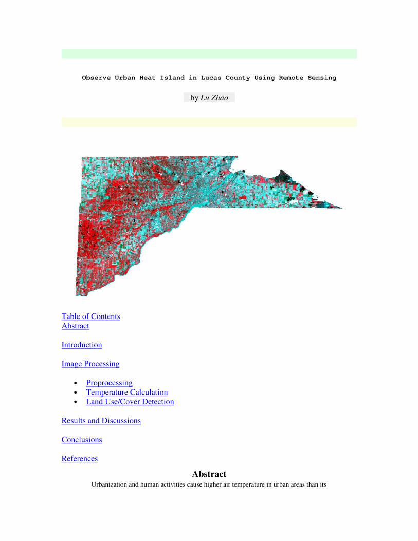
Lucas County, Ohio (figure 1) is an industrialized county and large amount of urban

activities may cause higher air temperature in urban areas than its surrounding areas,

which is called the phenomenon of urban heat island. In this project, Landsat7 TM+

image, which was acquired on July 1, 2000, and Landsat5 TM image, which was

obtained on July 13, 1984, were used to derive temperature and to extract land use/cover

information to see the effects of urban heat island in Lucas County. Landsat7 image has 8

bands and Landsat5 image has 7 bands. Both have one thermal band with the wavelength

range from 10.40 to 12.5?m. Because the electromagnetic wave within this range is

sensitive to temperature change, it can be used to derive temperature. All the 8 bands in

Landsat7 image and the 7 bands in Landsat5 image can be selected out to perform land

use/cover information extraction.

Figure 1 Lucas County

Image Processing

Figure 2 outlines the steps required to process remotely sensed data. Image processing

includes preprocessing, thematic information extraction and result interpretation. In this

project, two different thematic information extraction methods were applied, one being

temperature calculation and the other land use/cover information extraction. Two types of

resultant images were obtained: the temperature distribution image and the Land

use/cover map.

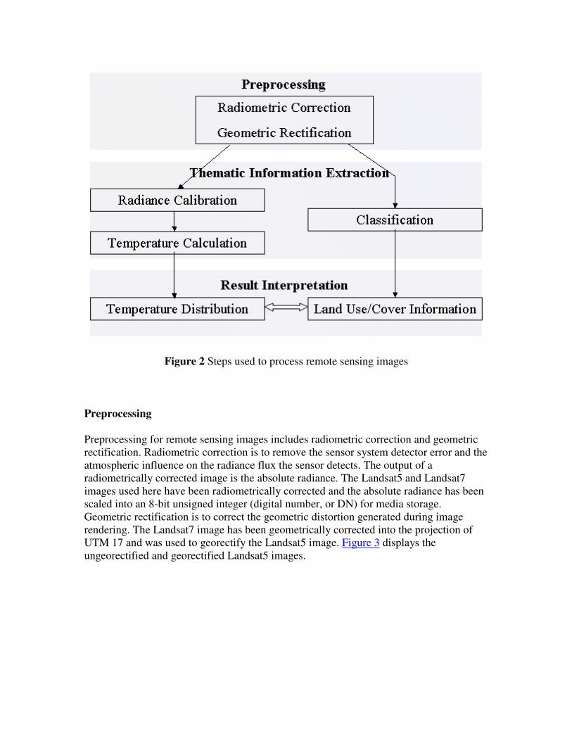
Figure 2 Steps used to process remote sensing images

Preprocessing

Preprocessing for remote sensing images includes radiometric correction and geometric

rectification. Radiometric correction is to remove the sensor system detector error and the

atmospheric influence on the radiance flux the sensor detects. The output of a

radiometrically corrected image is the absolute radiance. The Landsat5 and Landsat7

images used here have been radiometrically corrected and the absolute radiance has been

scaled into an 8-bit unsigned integer (digital number, or DN) for media storage.

Geometric rectification is to correct the geometric distortion generated during image

rendering. The Landsat7 image has been geometrically corrected into the projection of

UTM 17 and was used to georectify the Landsat5 image. Figure 3 displays the

ungeorectified and georectified Landsat5 images.

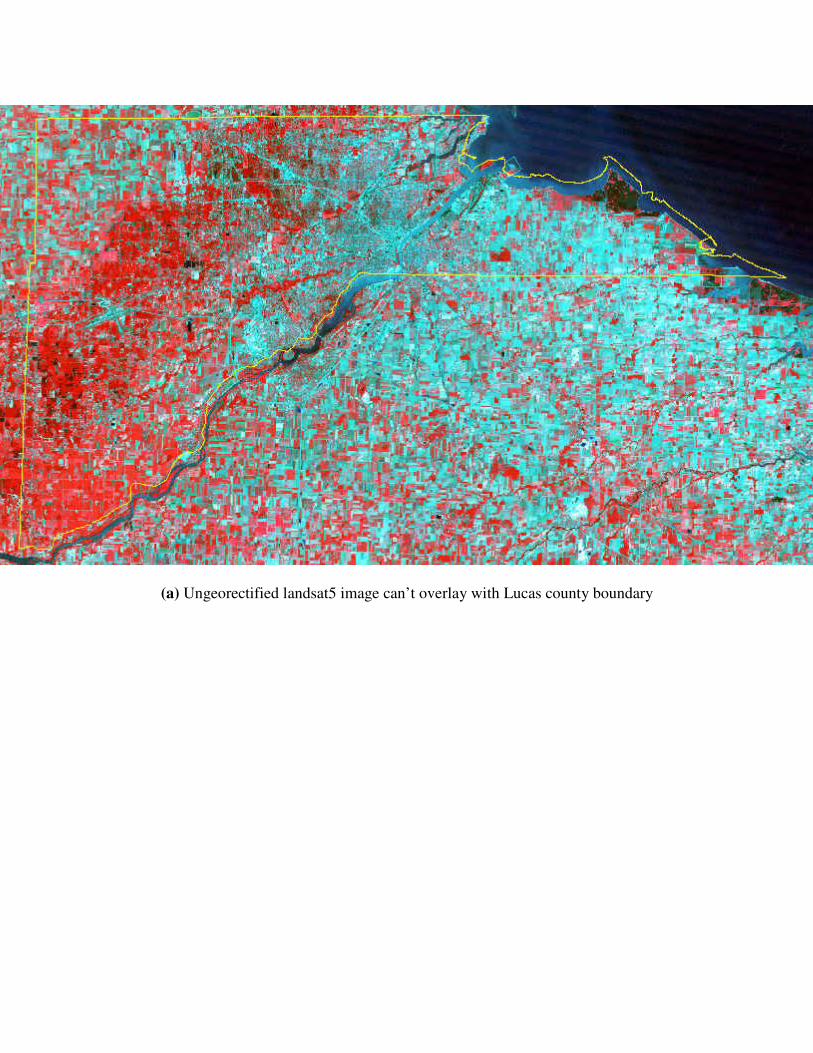
(a) Ungeorectified landsat5 image can’t overlay with Lucas county boundary

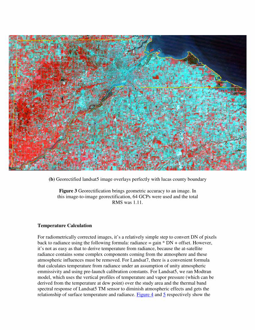
(b) Georectified landsat5 image overlays perfectly with lucas county boundary

Figure 3 Georectification brings geometric accuracy to an image. In

this image-to-image georectification, 64 GCPs were used and the total

RMS was 1.11.

Temperature Calculation

For radiometrically corrected images, it’s a relatively simple step to convert DN of pixels

back to radiance using the following formula: radiance = gain * DN + offset. However,

it’s not as easy as that to derive temperature from radiance, because the at-satellite

radiance contains some complex components coming from the atmosphere and these

atmospheric influences must be removed. For Landsat7, there is a convenient formula

that calculates temperature from radiance under an assumption of unity atmospheric

emmissivity and using pre-launch calibration constants. For Landsat5, we ran Modtran

model, which uses the vertical profiles of temperature and vapor pressure (which can be

derived from the temperature at dew point) over the study area and the thermal band

spectral response of Landsat5 TM sensor to diminish atmospheric effects and gets the

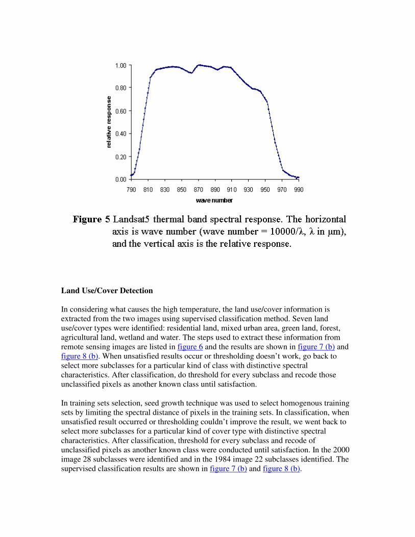
relationship of surface temperature and radiance. Figure 4 and 5 respectively show the

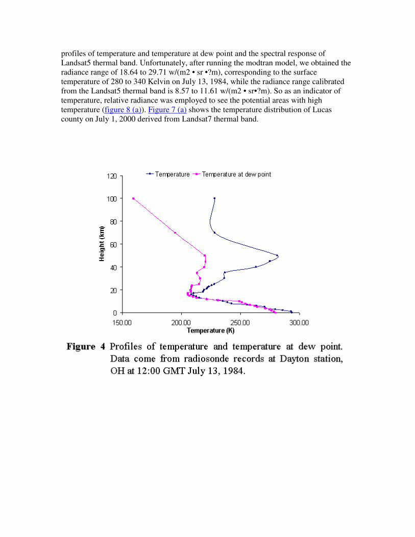
profiles of temperature and temperature at dew point and the spectral response of

Landsat5 thermal band. Unfortunately, after running the modtran model, we obtained the

radiance range of 18.64 to 29.71 w/(m2 • sr •?m), corresponding to the surface

temperature of 280 to 340 Kelvin on July 13, 1984, while the radiance range calibrated

from the Landsat5 thermal band is 8.57 to 11.61 w/(m2 • sr•?m). So as an indicator of

temperature, relative radiance was employed to see the potential areas with high

temperature (figure 8 (a)). Figure 7 (a) shows the temperature distribution of Lucas

county on July 1, 2000 derived from Landsat7 thermal band.

Land Use/Cover Detection

In considering what causes the high temperature, the land use/cover information is

extracted from the two images using supervised classification method. Seven land

use/cover types were identified: residential land, mixed urban area, green land, forest,

agricultural land, wetland and water. The steps used to extract these information from

remote sensing images are listed in figure 6 and the results are shown in figure 7 (b) and

figure 8 (b). When unsatisfied results occur or thresholding doesn’t work, go back to

select more subclasses for a particular kind of class with distinctive spectral

characteristics. After classification, do threshold for every subclass and recode those

unclassified pixels as another known class until satisfaction.

In training sets selection, seed growth technique was used to select homogenous training

sets by limiting the spectral distance of pixels in the training sets. In classification, when

unsatisfied result occurred or thresholding couldn’t improve the result, we went back to

select more subclasses for a particular kind of cover type with distinctive spectral

characteristics. After classification, threshold for every subclass and recode of

unclassified pixels as another known class were conducted until satisfaction. In the 2000

image 28 subclasses were identified and in the 1984 image 22 subclasses identified. The

supervised classification results are shown in figure 7 (b) and figure 8 (b).

Figure 6 Supervised classification method.

Figure 7 (a) Temperature distribution in Lucas County, Ohio on July

1, 2000. Temperature is derived from Landsat7 thermal data acquired

on the day. The minimum temperature is 10 °C and maximum

temperature is 51 °C.

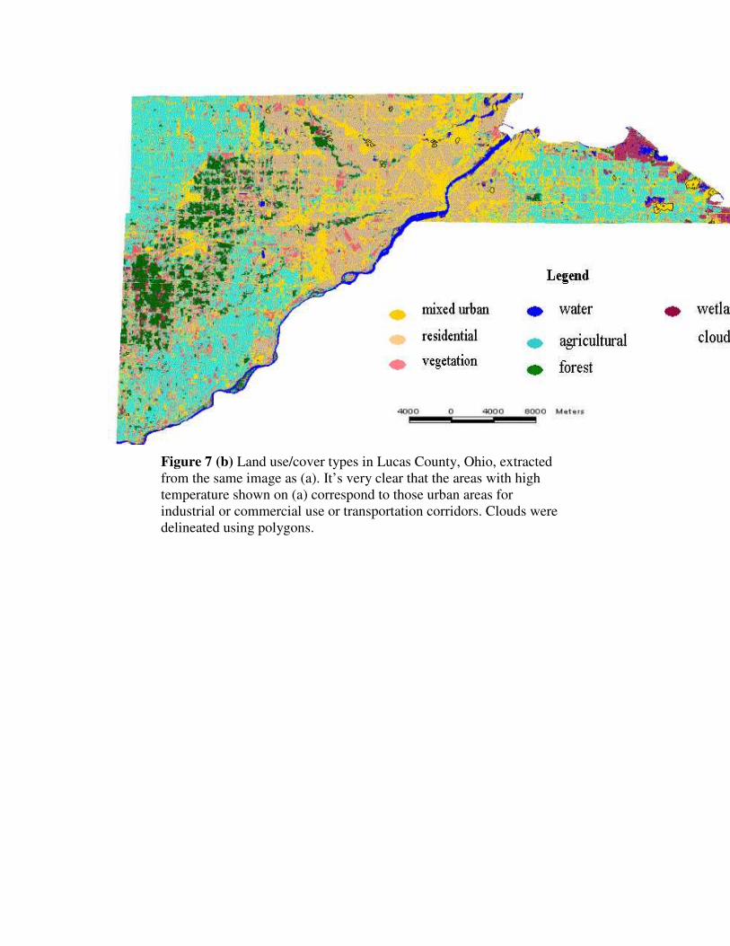
Figure 7 (b) Land use/cover types in Lucas County, Ohio, extracted

from the same image as (a). It’s very clear that the areas with high

temperature shown on (a) correspond to those urban areas for

industrial or commercial use or transportation corridors. Clouds were

delineated using polygons.

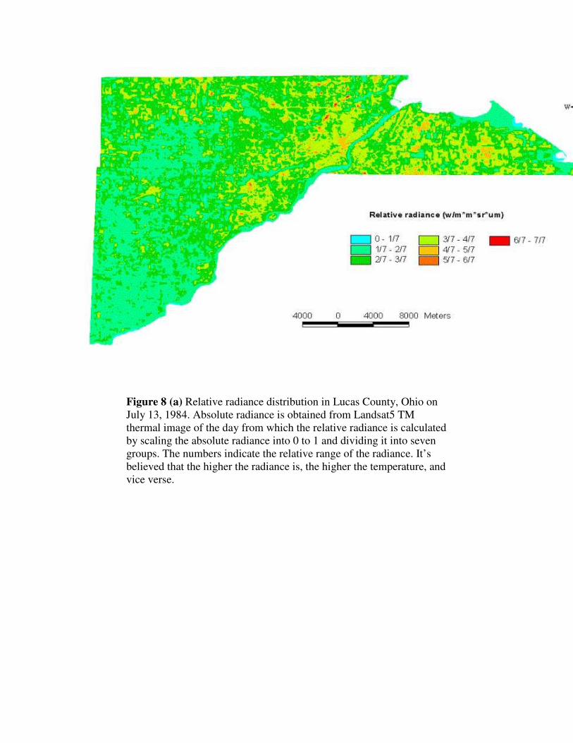
Figure 8 (a) Relative radiance distribution in Lucas County, Ohio on

July 13, 1984. Absolute radiance is obtained from Landsat5 TM

thermal image of the day from which the relative radiance is calculated

by scaling the absolute radiance into 0 to 1 and dividing it into seven

groups. The numbers indicate the relative range of the radiance. It’s

believed that the higher the radiance is, the higher the temperature, and

vice verse.

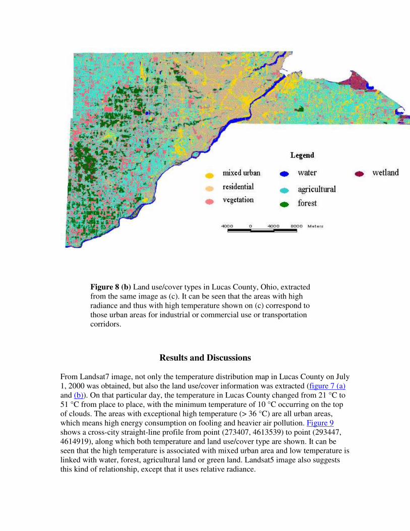
Figure 8 (b) Land use/cover types in Lucas County, Ohio, extracted

from the same image as (c). It can be seen that the areas with high

radiance and thus with high temperature shown on (c) correspond to

those urban areas for industrial or commercial use or transportation

corridors.

Results and Discussions

From Landsat7 image, not only the temperature distribution map in Lucas County on July

1, 2000 was obtained, but also the land use/cover information was extracted (figure 7 (a)

and (b)). On that particular day, the temperature in Lucas County changed from 21 °C to

51 °C from place to place, with the minimum temperature of 10 °C occurring on the top

of clouds. The areas with exceptional high temperature (> 36 °C) are all urban areas,

which means high energy consumption on fooling and heavier air pollution. Figure 9

shows a cross-city straight-line profile from point (273407, 4613539) to point (293447,

4614919), along which both temperature and land use/cover type are shown. It can be

seen that the high temperature is associated with mixed urban area and low temperature is

linked with water, forest, agricultural land or green land. Landsat5 image also suggests

this kind of relationship, except that it uses relative radiance.

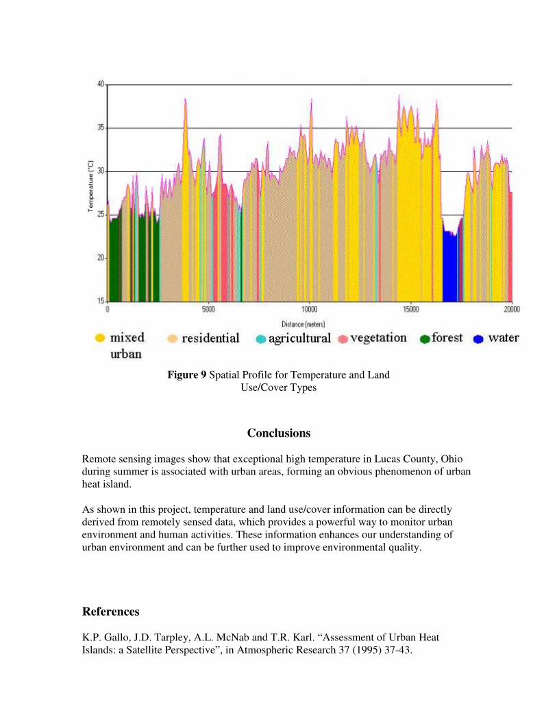
Figure 9 Spatial Profile for Temperature and Land

Use/Cover Types

Conclusions

Remote sensing images show that exceptional high temperature in Lucas County, Ohio

during summer is associated with urban areas, forming an obvious phenomenon of urban

heat island.

As shown in this project, temperature and land use/cover information can be directly

derived from remotely sensed data, which provides a powerful way to monitor urban

environment and human activities. These information enhances our understanding of

urban environment and can be further used to improve environmental quality.

References

K.P. Gallo, J.D. Tarpley, A.L. McNab and T.R. Karl. “Assessment of Urban Heat

Islands: a Satellite Perspective”, in Atmospheric Research 37 (1995) 37-43.

N. Magee, J. Curtis and G. Wendler. “The Urban Heat Island Effect at Fairbanks,

Alaska”, in Theoretical and Applied Climatology 64 (1999) 39-47.

Maurice G. Estes Jr., Virginia Gorsevski, Camille Russell, Dale Quattrochi, Jeffrey

Luvall. “The Urban Heat Island Phenomenon and Potential Mitigation Strategies”, at

http://www.asu.edu/caed/proceedings99/ESTES/ESTES.HTM.

John R. Jensen. 1996. Introductory Digital Image Processing: A Remote Sensing

Perspective.

Dale A. Quattrochi and Jeffrey C. Luvall. 1987. “High Spatial Resolution Airborne

Multispectral Thermal Infrared Data to Support Analysis and Modeling Tasks in EOS

IDS Project ATLANTA”, at http://www.ghcc.msfc.nasa.gov/atlanta/.

Robert Bornstein and Qinglu Lin. “Urban Heat Islands and Summertime Convective

Thunderstorms in Atlanta: Three Case Studies”, in Atmospheric Environment 34 (2000)

507-516.

Haider Taha. “Urban Climates and Heat Islands: Albedo, Evapotranspiration, and

Anthropogenic Heat”, in Energy and Buildings 25 (1997) 99-103.

Heat Island Group. 2000. at http://eetd.lbl.gov/HeatIsland/.

go back