Embed Size (px)
Citation preview
OBSERVATIONS OF SURFACE CURRENTS IN PANAY
STRAIT, PHILIPPINES
A DISSERTATION SUBMITTED TO THE GRADUATE DIVISION
OF THE UNIVERSITY OF HAWAI‘I AT MANOA IN PARTIAL
FULFILLMENT OF THE REQUIREMENTS FOR THE DEGREE OF
DOCTOR OF PHILOSOPHY
IN
OCEANOGRAPHY
December 2016
By
Charina Lyn A. Repollo
Dissertation Committee:
Pierre Flament, Chairperson
Mark Merrifield
Glenn Carter
Francois Ascani
Camilo Mora

We certify that we have read this dissertation and that, in our opinion, it is satisfac-
tory in scope and quality as a dissertation for the degree of Doctor of Philosophy in
Oceanography.
DISSERTATION COMMITTEE
Chairperson
i

Copyright 2016
by
Charina Lyn A. Repollo
ii

Acknowledgements
This thesis is the result of hard work whereby I have been accompanied and supported
by many people. This is an opportunity for me to express my gratitude for all of them.
I am indebted to the Office of the Naval Research (ONR) through the Philippine Strait
Dynamics Experiment (PhilEx) program for the funding support (grant N00014-09-1-
0807 to Pierre Flament). To the dedication and skill of the Captain and crew of the
R/V Melville and the many U.S. and Philippine students, technicians, volunteers, and
scientists who participated, assisted and helped in the fieldwork. Janet Sprintal provided
the moored shallow pressure gauges and ADCP data (ONR grant N00014-06-1-690), Craig
Lee provided the TRIAXUS data, and Julie Pullen provided the COAMPS winds.
I would like to express my sincere gratitude to my advisor, Pierre Flament, for his pa-
tience, motivation and intellectual support. His guidance helped me a lot in all the time
of research and writing of this thesis. Also his overly enthusiasm and integral view on
research and his dedication towards work has made a deep impression on me. To the
other members of my Ph.D. committee, Mark Merrifield, Glenn Carter, Francois Ascani
and Camilo Mora for their insightful comments and feedbacks.
I would not have succeeded without the help and support of teams from both the Physical
Oceanography Laboratory of the Marine Science Institute, University of the Philippines
and the Radio Oceanography Laboratory of the Department of Oceanography, University
of Hawai’i at Manoa with radar installation, operation and and maintenance. To Xavier
Flores-Vidal who supervised and helped in the field, and taught the initial processing of
the data. To Cedric Chavanne who picked me up from the airport when I first arrived at
UH and for all his helped on data processing. To Tyson Hilmer for calibration of HF radar
and Paul Lethaby for his help on PhilEx data management. Administrative assistance
was provided by the Ocean Office particularly, Kristin Momohara, Catalpa Kong, and
Lance Samura.
I thank my fellow labmates for the fruitful and stimulating discussions, for all the tiring
but fun fieldwork we had, and for the sleepless nights we were working together before
deadlines. To the graduate students of Radio Oceanography lab for the friendship and
sharing scientific discussions and feedback on this work, particularly Jake Cass, Victoria
Futch, Lindsey Benjamin, Alma Castillo, and Ian Quino Fernandez. My cohort, Sherril
iii

Leon Soon, Pavica Srsen, Saulo Soares, Huei-Ting Lin and Eunjun Kim. Also to Yannek
Meunier for sharing the opportunity working with radars in the Philippines.
I also appreciate the unyielding moral support from my fellow Filipino students and
friends, our family away from home. Lots of gratitude to Cesar Villanoy, who inspired
and paved the way to pursue this further studies. Together with Laura David, they play
a big part in this Ph.D. journey. Special thanks to Benedicte Dousset for all her support,
encouragement and inspiration. Her stories motivated and helped me a lot in staying on
the right track. To my family for their unconditional love and support.
And my heartfelt thanks to my husband, Jhobert whose patient love enabled me to
complete this work. To Hayden and Kaimalie for changing my life for the better. Words
cannot express how grateful I am for all your love and sacrifices on my behalf. You taught
me the good things that really matter in life.
Above all my deepest and sincere gratitude to OUR CREATOR for inspiring and guiding
this humble being.
Lastly, I would like to thank many individuals, friends and colleagues who have not been
mentioned here personally in making this educational process a success. I could not make
it without your support.
. . .
iv
Abstract
OBSERVATIONS OF SURFACE CURRENTS IN PANAY STRAIT,
PHILIPPINES
High Frequency Doppler Radar (HFDR), shallow pressure gauges (SPG) and Acoustic
Doppler Current Profiler (ADCP) time-series observations during the Philippine Straits
Dynamics Experiment (PhilEx) were analyzed to describe the tidal and mesoscale currents
in Panay Strait, Philippines.
Low frequency surface currents inferred from three HFDR (July 2008 – July 2009), reveal
a clear seasonal signal concurrent with the reversal of the Asian monsoon. A mesoscale
cyclonic eddy west of Panay Island is generated during the winter Northeast (NE) mon-
soon. This causes changes in the strength, depth and width of the intraseasonal Panay
coastal (PC) jet as its eastern limb. Winds from QuikSCAT and from a nearby air-
port indicate that these flow structures correlate with the strength and direction of the
prevailing local wind.
An intensive survey in February 8-9, 2009 using 24-hour of successive cross-shore Con-
ductivity - Temperature - Depth (CTD) sections, which in conjunction with shipboard
ADCP measurement show a well-developed cyclonic eddy characterized by near-surface
velocities of 50 cm/s. This eddy coincides with the intensification of the wind in between
Mindoro and Panay Islands generating a positive wind stress curl in the lee of Panay,
which in turn induces divergent surface currents. Water column response from the mean
transects show a pronounced signal of upwelling, indicated by the doming of isotherms
and isopycnals. A pressure gradient then is set up, resulting in the spin-up of a cyclonic
eddy in geostrophic balance. Evolution of the vorticity within the vortex core confirms
wind stress curl as the dominant forcing.
The Panay Strait constitutes a topographically complex system that is the locale of intense
tidal currents. The four major tidal constituents in the total energy spectra inferred from
sea level and current profile are K1, O1, M2, and S2. In terms of spatial variability, O1
and M2 are the dominant diurnal and semi-diurnal constituents, respectively. The diurnal
tide accounts for the highest variability over the shallow shelf while semi-diurnal tides
dominate over the deeper channel of the strait. In addition, inertial frequency peaks
v

and exhibits an unusually broad spectra between the clockwise and counterclockwise
components, possibly shifted by the vorticity of sub-inertial currents prevalent in the
region. Vertically, major tidal components in the velocity profile appear in two distinct
layers: at 110 m, 10.7% of the variance is associated with semi-diurnal tides, and at 470
m, 16.6% of the variance is due to diurnal tides (K1 and O1). Tidal current ellipses of
semi-diurnal constituents (M2 and S2) exhibit a dominant clockwise motion in time at
near-surface depth (110 m), indicative of downward energy propagation and implying a
surface energy source. These features observed in the ADCP deployed close to the sill may
explain the dominant semi-diurnal tide from the HFDR over the channel of the strait.
Comparison of incoherent to coherent tidal energy shows coherent energy is dominant over
the shallow Cuyo shelf for both diurnal and semi-diurnal tides while incoherent energy is
stronger over the channel, distinctly over the sill and the constricted part of the strait.
The incoherent portion of the tide is presumably attributable to the surface expression
of the internal tide which seems to be generated near the sill and then is topographically
steered west over the edge of the shallow shelf where incoherent energy is dominant.
vi
Contents
Acknowledgements iii
Abstract v
Contents vii
List of Figures ix
1 Introduction 1
2 Environmental and Instrumental Setting 5
2.1 Physical Setting . . . . . . . . . . . . . . . . . . . . . . . . . . . . . . . . 5
2.2 Instrumental Setting . . . . . . . . . . . . . . . . . . . . . . . . . . . . . 6
3 Low Frequency Surface Currents in Panay Strait, Philippines 13
3.1 Introduction . . . . . . . . . . . . . . . . . . . . . . . . . . . . . . . . . . 13
3.2 Instruments and Data Processing . . . . . . . . . . . . . . . . . . . . . . 15
3.3 Description of observations . . . . . . . . . . . . . . . . . . . . . . . . . . 16
3.3.1 Local wind variability . . . . . . . . . . . . . . . . . . . . . . . . 16
3.3.2 Surface ocean current patterns . . . . . . . . . . . . . . . . . . . . 17
3.3.3 Evidence for a wind-induced cyclonic eddy formation mechanism . 18
3.3.4 Dynamical analysis of the cyclonic eddy . . . . . . . . . . . . . . 21
3.3.4.1 Time lag between the wind forcing and the ocean response 22
3.4 Summary and Conclusion . . . . . . . . . . . . . . . . . . . . . . . . . . 25
4 Coastal sea response to atmospheric forcing in Panay Strait, Philippines 49
4.1 Abstract . . . . . . . . . . . . . . . . . . . . . . . . . . . . . . . . . . . . 49
4.2 Introduction . . . . . . . . . . . . . . . . . . . . . . . . . . . . . . . . . . 50
4.3 Methods . . . . . . . . . . . . . . . . . . . . . . . . . . . . . . . . . . . . 51
4.4 Results and Discussions . . . . . . . . . . . . . . . . . . . . . . . . . . . 53
4.4.1 Cruise Observational data . . . . . . . . . . . . . . . . . . . . . . 53
4.4.1.1 Velocity field . . . . . . . . . . . . . . . . . . . . . . . . 53
vii

Panay Lee (PL) Eddy . . . . . . . . . . . . . . . . . . . . . 54
Panay Tip (PT) Eddy . . . . . . . . . . . . . . . . . . . . 55
4.4.1.2 RIOP-09 Cruise Hydrographic data . . . . . . . . . . . . 56
Thalweg Distributions . . . . . . . . . . . . . . . . . . . . 56
4.4.1.3 T/S Distributions . . . . . . . . . . . . . . . . . . . . . 57
4.4.1.4 Coastal circulation and hydrographic response to atmo-spheric forcing . . . . . . . . . . . . . . . . . . . . . . . 58
4.4.1.5 Satellite Imagery . . . . . . . . . . . . . . . . . . . . . . 59
4.5 Summary and Conclusion . . . . . . . . . . . . . . . . . . . . . . . . . . 61
5 Barotropic and baroclinic tides in Panay Strait, Philippines 79
5.1 Abstract . . . . . . . . . . . . . . . . . . . . . . . . . . . . . . . . . . . . 79
5.2 Introduction . . . . . . . . . . . . . . . . . . . . . . . . . . . . . . . . . . 80
5.3 Methods . . . . . . . . . . . . . . . . . . . . . . . . . . . . . . . . . . . . 81
5.4 Results and Discussions . . . . . . . . . . . . . . . . . . . . . . . . . . . 83
5.4.1 Tidal components inferred from sea level . . . . . . . . . . . . . . 83
5.4.2 Horizontal structure of the tidal components inferred from HFDR 84
5.4.3 Vertical structure of the tidal component inferred from ADCP . . 86
5.4.4 Coherent tides . . . . . . . . . . . . . . . . . . . . . . . . . . . . . 87
5.4.5 Ratio of Incoherent to Coherent Energy . . . . . . . . . . . . . . 88
5.5 Summary and Conclusion . . . . . . . . . . . . . . . . . . . . . . . . . . 89
6 Summary and Conclusion 109
Bibliography 112
viii

List of Figures
1.1 Bathymetric map showing the major straits and basins of the Philippinearchipelago. Bathymetry contours are in meters. . . . . . . . . . . . . . . 4
2.1 Bathymetry of study area and the limits of 75% HFDR data coverageindicated by red thick broken line. Locations of observations are marked:HFDR by red circles, SPG by yellow diamonds, ADCP by magenta square,TRIAXUS survey transects by green lines, and the nearby Caticlan airportby green star. . . . . . . . . . . . . . . . . . . . . . . . . . . . . . . . . . 9
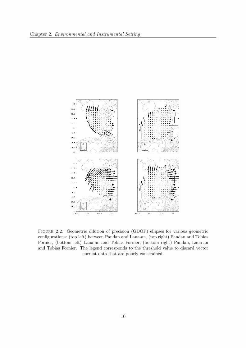
2.2 Geometric dilution of precision (GDOP) ellipses for various geometric con-figurations: (top left) between Pandan and Laua-an, (top right) Pandanand Tobias Fornier, (bottom left) Laua-an and Tobias Fornier, (bottomright) Pandan, Laua-an and Tobias Fornier. The legend corresponds tothe threshold value to discard vector current data that are poorly con-strained. . . . . . . . . . . . . . . . . . . . . . . . . . . . . . . . . . . . . 10
2.3 Temporal coverage of the three HF radar sites and of the combined vectorcurrents. The thickness corresponds to the percentage of grid points withdata. The percentage of data obtained during the operation is 70.3% forPandan, 72% for Laua-an, 70.6% for Tobias and 79.4% for the vector currents. 11
2.4 Cross-correlation between radial currents from pairs of sites (left column),and cosine of the angle between the sites (right column) for Pandan andLaua-an (top row), Pandan and Tobias (middle row) and Lauan-an andTobias (bottom row). The circle where the angle between the two sites is90◦ is overlaid for reference. . . . . . . . . . . . . . . . . . . . . . . . . . 12
3.1 Temporal coverage of the HFDR combined vector currents, ADCP currentprofile, QuikSCAT, and Caticlan Airport winds. The thickness correspondsto the percentage of grid points with data. The percentage of data 79.4%for the vector currents, 100% for current profile, 98.7% for QuikSCAT and99.8% for the airport wind. The thick solid line marked the RIOP-09 cruisein February 2009. . . . . . . . . . . . . . . . . . . . . . . . . . . . . . . . 27
3.2 Rotary power spectra of hourly (dark gray) and 6-day medianed (lightgray) HFDR data averaged over an area with more than 75% temporalcoverage. Major tidal constituents (O1, K1, M2 and S1) and inertial fre-quency (f) are indicated on the top x-axis. . . . . . . . . . . . . . . . . . 28
ix
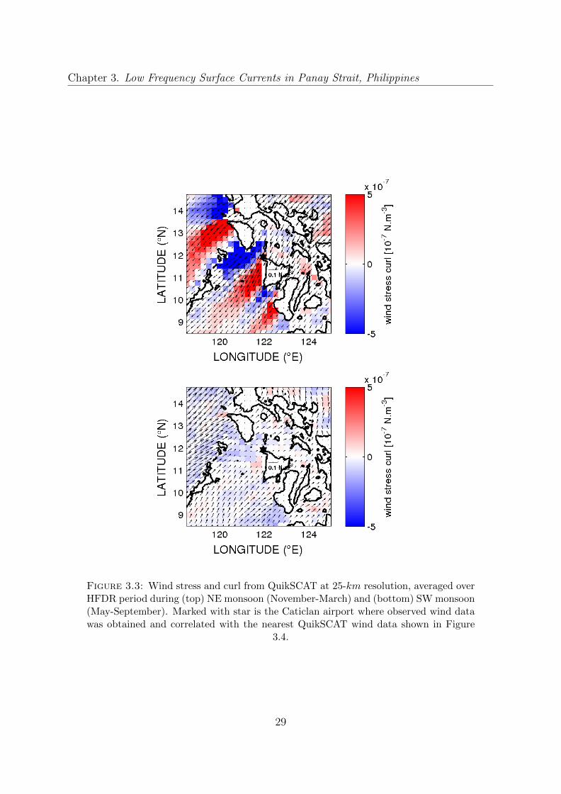
3.3 Wind stress and curl from QuikSCAT at 25-km resolution, averaged overHFDR period during (top) NE monsoon (November-March) and (bottom)SW monsoon (May-September). Marked with star is the Caticlan airportwhere observed wind data was obtained and correlated with the nearestQuikSCAT wind data shown in Figure 3.4. . . . . . . . . . . . . . . . . . 29
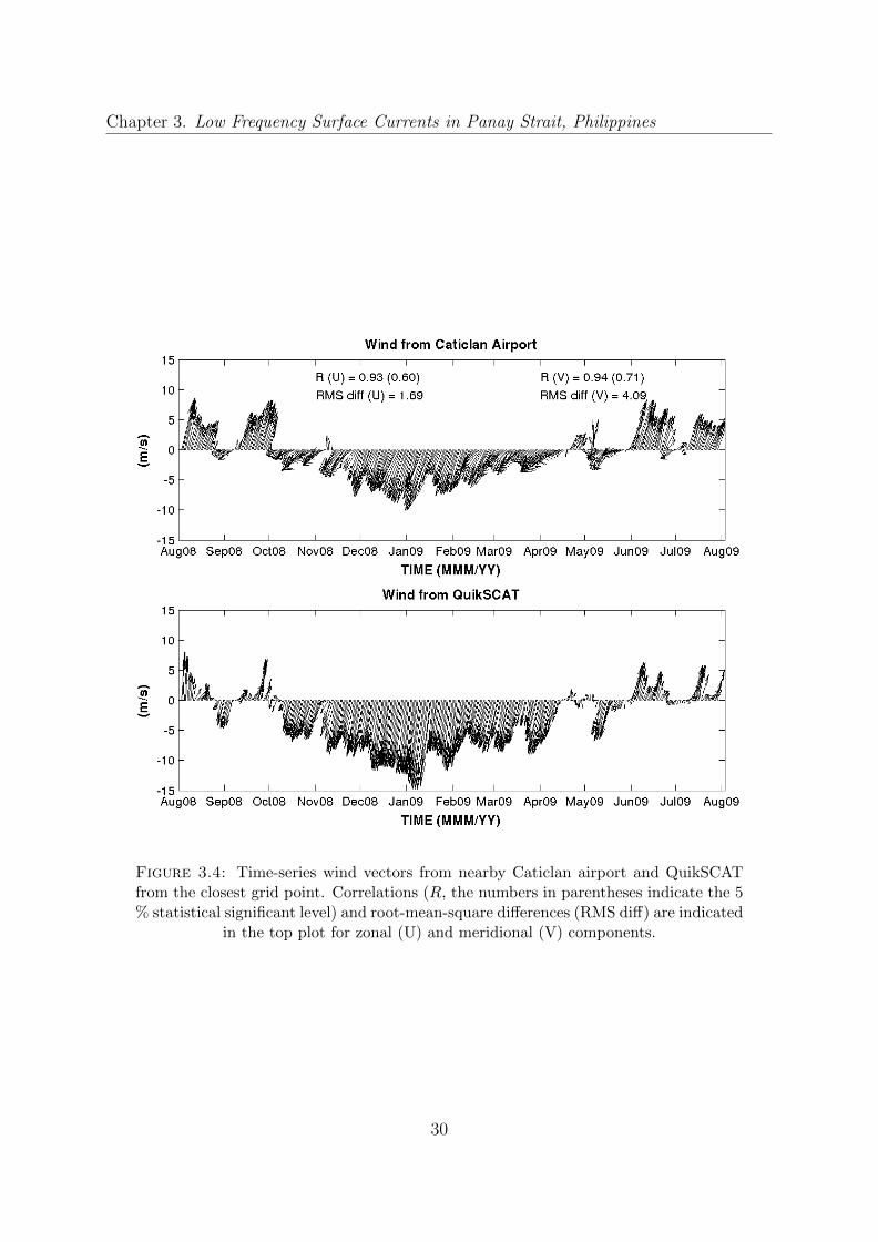
3.4 Time-series wind vectors from nearby Caticlan airport and QuikSCAT fromthe closest grid point. Correlations (R, the numbers in parentheses indi-cate the 5 % statistical significant level) and root-mean-square differences(RMS diff) are indicated in the top plot for zonal (U) and meridional (V)components. . . . . . . . . . . . . . . . . . . . . . . . . . . . . . . . . . . 30
3.5 Mean flow overlaid with speed contoured in cms−1 during (top) NE mon-soon and (bottom) SW monsoon. Three transects are marked accordinglyalong which mean surface flow profiles are shown in Figure 3.6. . . . . . . 31
3.6 Time series profiles of (top) PC jet and (bottom) cyclonic eddy. Positive(negative) values indicate flow towards the north (south). The line colorand type corresponds to three transects in Figure 3.5. . . . . . . . . . . . 32
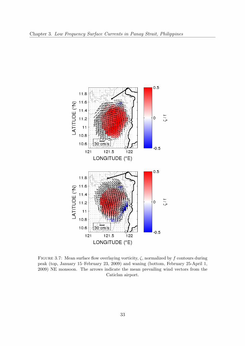
3.7 Mean surface flow overlaying vorticity, ζ, normalized by f contours duringpeak (top, January 15–February 23, 2009) and waning (bottom, February25-April 1, 2009) NE monsoon. The arrows indicate the mean prevailingwind vectors from the Caticlan airport. . . . . . . . . . . . . . . . . . . . 33
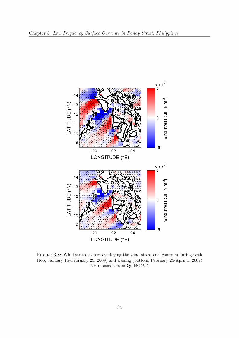
3.8 Wind stress vectors overlaying the wind stress curl contours during peak(top, January 15–February 23, 2009) and waning (bottom, February 25-April 1, 2009) NE monsoon from QuikSCAT. . . . . . . . . . . . . . . . . 34
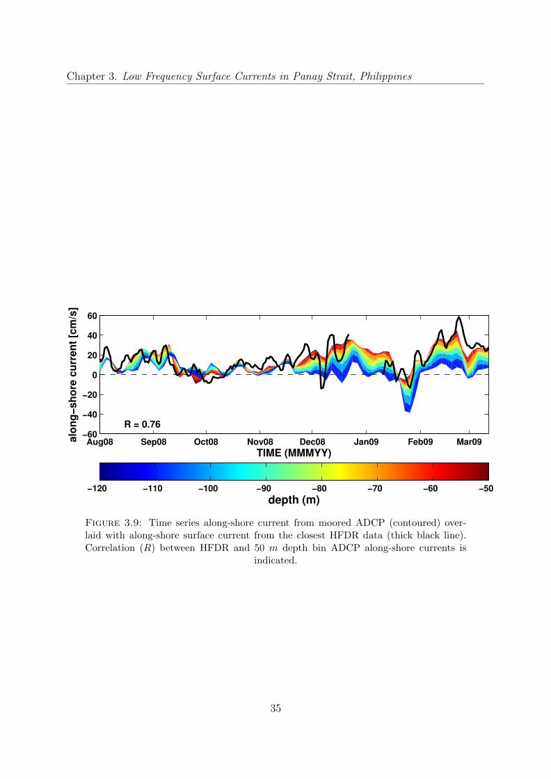
3.9 Time series along-shore current from moored ADCP (contoured) overlaidwith along-shore surface current from the closest HFDR data (thick blackline). Correlation (R) between HFDR and 50 m depth bin ADCP along-shore currents is indicated. . . . . . . . . . . . . . . . . . . . . . . . . . . 35
3.10 The Coupled Ocean/Atmosphere Mesoscale Prediction System (COAMPS)left) 10 m mean wind, wind vectors plotted over wind speed contour (ms−1
and right) mean wind stress curl contour (Nm−3) from the 9 km computa-tional grids for the Regional Intensive Observational Period, February toMarch 2009 (RIOP-09). . . . . . . . . . . . . . . . . . . . . . . . . . . . . 36
3.11 Surface wind speeds derived from an Envisat Synthetic Aperture Radar(SAR) image with wind vectors from the Navy Operational Global Analysisand Prediction System (NOGAPS) model for 0141 UTC 7 Mar 2009. . . 37
3.12 Snapshots of surface current overlaid with contoured Ekman pumping ve-locity calculated from (left) QuikSCAT and (right) COAMPS wind. Windvectors at Caticlan airport (thick arrows) are also indicated. . . . . . . . 38
3.13 Mean surface current overlaid with contoured mean divergence for Febru-ary to March 2009 (RIOP-09). . . . . . . . . . . . . . . . . . . . . . . . . 39
x
3.14 Vertical transect of mean (top) temperature, (middle) density, and (bot-tom) along-shore flow from the shipboard ADCP across the Panay Straitduring the hydrographic survey (February 8-9, 2009) shown in Figure 2.1.The mean near-surface along-shore flow vectors are indicated above. . . . 40
3.15 HFDR mean surface current overlaid with contoured mean vorticity forFebruary to March 2009 (RIOP-09). . . . . . . . . . . . . . . . . . . . . . 41
3.16 Scatterplots of mean (top) divergence vs. Ekman pumping velocity, and(bottom) vorticity vs. Ekman pumping velocity. Divergence and vortic-ity were calculated using HFDR data while Ekman pumping velocity wascalculated using COAMPS from the region inside the box shown in Figure3.13 and Figure 3.15 during February to March 2009 (RIOP-09). . . . . . 42
3.17 Time series of vorticity balance terms (Equation 3.3) averaged over thevortex core. The β term is vertically exaggerated. Vertical dotted linesindicate the snapshots in Figure 3.18 and Figure 3.19. . . . . . . . . . . . 43
3.18 Snapshots of the terms of the surface vorticity balance (Equation 3.3),overlaid with surface currents. From left to right, Lagrangian rate of changeof vorticity, vortex stretching, residual, and Beta-effect terms. The timesof snapshots are indicated on the y-axis of the first column. . . . . . . . . 44
3.19 Snapshots of the terms of the surface vorticity balance (Equation 3.3),overlaid with surface currents. From left to right, Lagrangian rate of changeof vorticity, vortex stretching, residual, and Beta-effect terms. The timesof snapshots are indicated on the y-axis of the first column. . . . . . . . . 45
3.20 Time-series of divergence (top) and relative vorticity (bottom) overlaidwith scaled Ekman pumping velocity. All terms were normalized by f . . 46
3.21 Vorticity overlaid with time integral of wind stress curl and divergenceconfined within the Ekman layer (HE = 32 m). . . . . . . . . . . . . . . 47
3.22 Time series (top) sea level and (bottom) temperature anomaly from Pan-dan and Tobias Fornier shallow pressure gauges. . . . . . . . . . . . . . . 48
4.1 Bathymetry and TRIAXUS survey transects (solid thick line in red, greenand blue) for the Panay Strait region during RIOP-09 in February 8-15,2009. Marked are the 3 HFDR, SPG located just in front of the north andsouth HFDR sites, moored ADCP and the nearby Caticlan airport. The200m, 500m, and 1000m isobaths are indicated by thin gray lines. . . . . 63
4.2 Bathymetry and shipboard ADCP tracks for the Panay Strait region duringRIOP-09 in February 8-15, 2009. The survey region over Pandan bay closeto the coast was repeatedly mapped for over a 24-hour period. The 200m,500m, and 1000m isobaths are indicated by thin gray lines. . . . . . . . . 64
4.3 (top) Surface current from HFDR and from shipboard ADCP. (bottom)Major surface flows observed are the cyclonic Panay eddy, the northwardPanay coastal jet and the small cyclonic eddy at the tip of Northwest Panaypeninsula. . . . . . . . . . . . . . . . . . . . . . . . . . . . . . . . . . . . 65
xi
4.4 Near-surface current from shipboard ADCP 12 m depth bin and the pre-vailing wind from the Caticlan airport during two successive surveys on(top) February 8-10, 2009 and (bottom) February 12-15, 2009. The sam-pling time from start to end are shown with increasing lighter shadings.The current and wind vectors are color-coded accordingly. . . . . . . . . 66
4.5 Measured tidal height at Pandan, Antique, Philippines for February 2009.The location of the shallow pressure gauge is indicated in Figure 4.1 markedwith red dot. The blue line represents the tidal height during the surveyperiod, February 8-14, 2009 while the red portion is the tidal height whenthe two TRIAXUS sections were covered. . . . . . . . . . . . . . . . . . . 67
4.6 (A) Measured sea level at Pandan, Antique, Philippines for the periodof February 9-10, 2009. The colored portion of the tidal series are thetidal height during the period that multiple iterations of each cross-shoretransect were covered, from transect 1 to 4 as colored accordingly. Currentvectors during (B) flood and (C) ebb tide from 10 m, 50 m and 100 m(colored) and from 130 m and 150 m (gray) are shown. The color shadefrom light to dark as it goes deeper. . . . . . . . . . . . . . . . . . . . . . 68
4.7 Speed (left panel) and direction (right panel). Left panel were sampledduring flood tide while the right panel were sampled during ebb tide. Pos-itive values are from northeast to northwest direction and negative valuesare from southeast to southwest direction. -180(◦ and 180(◦ is westwardwhile 0(◦ is eastward. . . . . . . . . . . . . . . . . . . . . . . . . . . . . . 69
4.8 (A) Measured sea level at Pandan, Antique, Philippines for the periodof February 13-14, 2009. The colored portion of the tidal series are thetidal height during the period that the (B) tip of Panay and (C) multipleiterations of each survey tracks were performed, as colored accordingly.The near-surface currents from 12 m depth bin were labelled with time inhours, left panel (C) were sampled during ebb tide while the right panel(C) during spring tide. The prevailing mean daily wind during February13-15, 2009 from the nearby airport is shown (blue to green color). . . . . 70
4.9 (A) Measured sea level at Pandan, Antique, Philippines for the periodof February 13-14, 2009. The colored portion of the tidal series are thetidal height during flood (B) and ebb (C) tides TRIAXUS survey. Theoverlapping tracks were colored in gray during flood tide. The points arelabelled with time in hours. (D) Temperature, salinity, (E) density andchlorophyll profiles from survey tracks covered above. Vertical dotted linesindicate the time on the tracks. . . . . . . . . . . . . . . . . . . . . . . . 71
4.10 (A) Wind vectors at Caticlan airport, surface current vectors and (B) ve-locity profile (top: speed, bottom: direction) from the shipboard-mounted150-KHz ADCP system. For direction, positive values are from northeastto northwest direction and negative values are from southeast to southwestdirection. -180(◦ and 180(◦ is westward while 0(◦ is eastward. (C) Temper-ature, salinity, (D) density and chlorophyll concentration from CTD andfluorometer attached to TRIAXUS through the thalweg section. . . . . . 72
xii

4.11 (A) The TRIAXUS survey tracks for Panay Strait region during February8-14, 2009. (B) The Temperature and salinity obtained by CTD attachedon TRIAXUS and (C) overlaid by temperature and salinity from CTD castsduring March 2009 regional cruise showing characteristic water masses fromPacific Ocean and Tablas Strait. . . . . . . . . . . . . . . . . . . . . . . . 73
4.12 (top) 6-day medianed sea level anomalies (cm) and temperature (red line,(◦C/10) ) from Pandan shallow pressure gauge overlaid with wind vectors(ms−1) from the closest QuikSCAT data. Correlations, R between zonal,U and meridional, V wind component with sea level (left) and temperature(right) are indicated on the top of the plot. (bottom) The correspondingsalinity (psu) anomalies. . . . . . . . . . . . . . . . . . . . . . . . . . . . 74
4.13 The 24-hour mean velocity profile from the NW corner of Panay Island.(A) Current vectors from 10m, 75m, and 125m with increasingly lightershadings. (B) On top is the speed while on the bottom is the direction.Positive values are from northeast to northwest direction (white to redcontour) and negative values are from southeast to southwest direction(white to blue contour). The y-axis is the distance marked in Figure 4.23 A. 75
4.14 Sea surface Temperature (SST) for the Philippine Archipelago. The imageis a 1 km composite of MODIS Aqua sensor image for the period February 7to 13, 2009 (top) and the 6 km daily Group for High Resolution Sea SurfaceTemperature (GHRSST) Level 4 SST data (daily mean values provided byPhysical Oceanography DAAC (http://podaac.jpl.nasa.gov/dataset/UKMO-L4HRfnd-GLOB-OSTIA) averaged over the same time period (bottom). . 76
4.15 Mean profile of temperature, salinity and chlorophyll concentration acrossthe PL eddy during the hydrographic survey (February 8-9, 2009). . . . . 77
4.16 The Sea Surface Temperature (SST) 1 km MODIS Aqua Imagery compos-ite images and the Chlorophyll concentration merged (MODIS, MERIS,SEAWIFS) composite images of Philippine archipelago for February 20 to26, 2009. . . . . . . . . . . . . . . . . . . . . . . . . . . . . . . . . . . . . 78
5.1 Map of study area. Bathymetry contours are in meters. The color barrepresents color depth in meters. Instrument locations are indicated asfollows: HFDR (red circle), moored ADCP (magenta square), and SPG(yellow diamond). The magenta dashed lines indicates 75 % coverage ofthe HFDR. . . . . . . . . . . . . . . . . . . . . . . . . . . . . . . . . . . 90
5.2 Temporal coverage of the instruments. The thickness corresponds to thepercentage of grid points with data. . . . . . . . . . . . . . . . . . . . . . 91
5.3 Power spectral density of the time series overlap of a)Pandan and b) TobiasFornier SPG. . . . . . . . . . . . . . . . . . . . . . . . . . . . . . . . . . 92
5.4 Increment variance (%) of major tidal constituents. The first 4 markeddots indicate the variance of (1) K1, (2) K1 and O1, (3) K1, O1, and M2,(4) K1, O1, M2, and S2. . . . . . . . . . . . . . . . . . . . . . . . . . . . 93
xiii

5.5 Rotary power spectra for one year of HFDR data over 212 grid points withmore than 75% temporal coverage. Major tidal constituents and inertialfrequency, fi are indicated on the top x-axis, indicated by vertical dottedlines. . . . . . . . . . . . . . . . . . . . . . . . . . . . . . . . . . . . . . . 94
5.6 Variance explained by 4 major tidal constituents (K1, O1, M2, and S2). . 95
5.7 Variance explained by (top) diurnal and (bottom) semidiurnal tidal con-stituents. . . . . . . . . . . . . . . . . . . . . . . . . . . . . . . . . . . . . 96
5.8 Mean kinetic energy, eddy kinetic energy and tidal kinetic energy. . . . . 97
5.9 Contribution of tidal currents to the (A) mean kinetic energy, Rtmke andthe (B) eddy kinetic energy, Rteke. . . . . . . . . . . . . . . . . . . . . . . 98
5.10 Contribution of diurnal tidal currents, (top) O1 and (bottom) M2 to the to-tal mean kinetic energy, Rtmke and the eddy kinetic energy, Rteke averagedfor over a year. . . . . . . . . . . . . . . . . . . . . . . . . . . . . . . . . 99
5.11 Rotary power spectra from vertically averaged frequency spectra fromADCP. Major tidal constituents and inertial frequency, fi are indicatedon the top x-axis, indicated by vertical dotted lines. . . . . . . . . . . . . 100
5.12 Variance explained by 4 major constituents (K1, O1, M2, and S2). . . . . 101
5.13 Mean current, eddy, and tidal current kinetic energies. . . . . . . . . . . 102
5.14 Contribution of tidal currents to the (A) mean kinetic energy, Rtmke andthe (B) eddy kinetic energy, Rteke. . . . . . . . . . . . . . . . . . . . . . . 103
5.15 (top to bottom) O1, K1, M2, and S2 (bottom) (left column) ellipses, (mid-dle column) major axis amplitude, and (right column) Greenwich phase ofHFDR tidal current. Counterclockwise and clockwise ellipses are plottedin red and blue respectively. The phase is defined as the lag of the max-imum current (along the northern semi-major axis) with respect to theastronomical phase of M2 at 0◦E. . . . . . . . . . . . . . . . . . . . . . . 104
5.16 O1, K1, (top) M2, and S2 (bottom), averaged ellipses with depth Counter-clockwise and clockwise ellipses are plotted in red and blue respectively. . 105
5.17 Ratio of incoherent to coherent diurnal and semidiurnal tides as observedin surface current record. . . . . . . . . . . . . . . . . . . . . . . . . . . . 106
5.18 Rotary power spectra for one year of residual HFDR data over 212 gridpoints with more than 75 % temporal coverage. Major tidal constituentsand inertial frequency, fi are indicated on the top x-axis, indicated byvertical dotted lines. . . . . . . . . . . . . . . . . . . . . . . . . . . . . . 107
5.19 Ratio of incoherent to coherent diurnal and semidiurnal tides as observedin the current profile record. . . . . . . . . . . . . . . . . . . . . . . . . . 108
xiv

Chapter 1
Introduction
Along the Pacific Ocean’s western margins lie the Philippine Islands, a northern seg-
ment of an archipelago stretching from Southeast Asia to Australia. This island chain
constrains the flow between the tropical western Pacific and eastern Indian oceans into
a complex configuration of narrow straits and seas of various sizes. This area is sub-
ject to the reversal of the Asian monsoon, inter-annual variations such as the El Nino
Southern Oscillation (ENSO), and episodic occurrences (e.g monsoon surges and tropical
cyclones), making it challenging to observe and model. The Office of Naval Research
(ONR) sponsored the PhilEx with a goal of exploring the oceanography and dynamics in
the narrow straits and deep basins of the Philippines using integrated in-situ and remote
observational methods with global and regional model components [Gordon and Villanoy,
2011].
Flows through Philippine straits are modulated by a range of processes at different spatial
and temporal scales. Previous work in the region using ship-drift data [Wrytki, 1961]
identified the role of the Asian monsoon in directing the surface flow between the South
China Sea (SCS) and the Sulu Sea through the Mindoro Strait-Panay Strait complex
(Figure 1.1). During the peak of the Northeast (NE: December-March) monsoon, Pacific
Ocean surface waters enter westward through the Surigao and San Bernardino Straits
into the Sulu Sea, and exit northward through Mindoro into the SCS and southward
through Sibutu Passage into the Sulawesi Sea [Wrytki, 1961]. During the Southwest (SW:
June–September) monsoon the surface flow is southward from the SCS in Mindoro Strait,
1

Chapter 1. Introduction
and circulation within the Sulu Sea is cyclonic [Wrytki, 1961]. However, observations from
ship drift records are too scanty and do not give a complete picture of the circulation.
Pullen et al. [2008] used a one-way coupled high-resolution atmosphere and ocean sim-
ulation of the Philippine region, to highlight the importance of topographically-induced
wind shear in forcing the surface ocean. Monsoon surge events prevalent during winter
induce the generation and migration of pairs of counter-rotating oceanic eddies caused
by intensified wind jets and wakes in the lee of Luzon and Mindoro. Comparison of high-
resolution model and observed near-surface currents in the Philippine Archipelago, also
confirmed the strong eddy flow pattern within Mindoro Strait and west of Panay [Han
et al., 2009].
A time series of observed velocity and properties from moored ADCP in Mindoro and
Panay Straits over a year (2008) revealed a complex response to the surface monsoonal
forcing [Sprintall et al., 2012]. ADCP measurements in the upper layer in Mindoro Strait
show a distinctly seasonal cycle with northward flow during the boreal summer SW mon-
soon and southward flow during the winter NE monsoon. In contrast, upper layer flow
in Panay Strait is intra-seasonal with no clear monsoonal relationship. It has been sug-
gested that regional wind forcing dynamics are responsible for the upper layer transport
variability. Local winds shift the location of the jets and eddies prevalent in the region,
and subsequently lead to intermittent reversals and more variable upper layer transport
observed in Panay Strait [Sprintall et al., 2012].
Previous studies in Panay Strait, however were inferred from models with known errors,
such as coarse resolution, inaccuracy of forcing fields, incorrect heat flux and freshwater
parameterizations, and lack of river outflow [Han et al., 2009]. At the same time, missing
data in the upper 40m from the moored ADCP [Sprintall et al., 2012] make the connection
of the near-surface flow to the monsoon variability problematic. The vertical profiles of
currents by single-point moored ADCP also compromise the estimation of across-passage
transport [Sprintall et al., 2012]. ADCP data therefore do not fully resolve the spatial
and temporal variability of the surface layer flow.
Intensive observations of Panay Strait were carried out to qualitatively and quantita-
tively describe the mesoscale spatial structure and temporal variability of the surface
current within the strait. Measurements of surface currents from three HFDR during the
PhilEx program were analyzed to characterize the dominant low-frequency surface flows,
2

Chapter 1. Introduction
investigate its forcing mechanisms, and determine the structure of the barotropic and
baroclinic tides. Analyses were done in conjunction with the wind data from QuikSCAT
and from a nearby airport, two SPG, one ADCP mooring, hydrographic data, modeled
wind from Coupled Ocean/Atmosphere Mesoscale Prediction System (COAMPS), and
satellite images of sea surface temperature, ocean color, and wind speed.
3

Chapter 1. Introduction
Figure 1.1: Bathymetric map showing the major straits and basins of the Philippinearchipelago. Bathymetry contours are in meters.
4
Chapter 2
Environmental and Instrumental
Setting
2.1 Physical Setting
The Panay Strait serves as the major pathway of South China Sea water entering through
Mindoro Strait into the deep Sulu Sea basin (Figure 2.1). The strait is bounded by the
coast of Panay Island on the east and the Palawan Island chain on the west. Along
Panay, the shelf is narrow (less than 10 km) while the northern Palawan shelf extends
eastward as the shallow Cuyo Shelf. This then forms a deep channel close to the coast
of Panay, based on 100 m isobath with sill depth of about 570 m deep. On the shelf lies
the low-lying Cuyo Group of Islands and extensive reefs.
The flow within the strait is modulated by a range of processes such as tidal variations,
seasonal reversal of the monsoon, sea level variations between SCS and the Pacific Ocean,
interannual variations such as ENSO, and episodic occurrence of monsoon surges and
tropical cyclones [White et al., 2003; McClean et al., 2005; Pullen et al., 2008; Han et al.,
2009; May et al., 2011].
5
Chapter 2. Environmental and Instrumental Setting
2.2 Instrumental Setting
Three short-wave ocean current-mapping radars were deployed along the west coast of
Panay Island to measure surface circulation from July 2008 to August 2009 during the
PhilEx program (Figure 2.1). This observational component aims to quantitatively de-
scribe the mesoscale spatial structure and the temporal variability of the surface currents
within Panay Strait. The antenna at each site are grouped in a receive array and a
transmit array. The northernmost and southernmost sites located in Pandan and Tobias
Fornier, respectively, include a linear array of 12 receiving antenna, whereas the middle
site at Laua-an consists of a linear array of 8 receiving antenna. The four transmit an-
tenna arranged in a rectangular array formed a beam toward the ocean, and a null in the
direction of the receive antennas, to reduce the direct path energy. This also reduced the
range away from the beam axis.
For each HFDR, radial currents are measured by transmitting a radio signal at 12 Mhz
frequency. The radio waves are reflected by surface gravity waves having half the elec-
tromagnetic wavelength (λ =25 m, Bragg scattering) of the transmitted signal, and are
then recorded by the receive antenna. The backscattered radio waves generate a Doppler
shifted signal in which the frequency shift is used to calculate the currents moving toward
or away from the site. Vector currents were estimated on a 5 km Cartesian grid by least-
square fitting zonal and meridional components of the radial measurements from three
sites within a 5 m search radius. The range of HFDR data used for analysis was limited
by geometric dilution of precision (GDOP, Figure 2.2) that resulted from the normal
velocity component being poorly constrained near the baseline between the sites and the
azimuthal component poorly constrained far from the sites. Vector current estimations
with a GDOP greater than 0.5 were discarded [Chavanne et al., 2007].
Periodically missing observations at long ranges (presumably due to diurnal variation
of ionospheric propagation and absorption) were resolved by linear interpolation carried
out on the vector currents (see Appendix B, after [Chavanne et al., 2007]). The least
square analysis was carried out on the interpolated time series. Temporal coverage of
the individual sites and of vector current estimations are shown in (Figure 2.3). Vector
currents with 75% temporal coverage were used for analysis.
6

Chapter 2. Environmental and Instrumental Setting
Failures in HFDR occurred at sites due to electrical power loss primarily because of
burned power cables and generator failures during black-outs. In times when data were
lost from one site, two sites were used to calculate vector currents. During the deployment
period, the largest data loss was during the bistatic calibration performed from December
22, 2008 to January 9, 2009.
Data quality was evaluated by cross correlations between radial currents from pairs of sites
(Figure 2.4). If along-baseline and across-baseline current components were uncorrelated
with equal variance, the correlation pattern would follow that of the cosine of the angle
between the two sites, indicating accuracy of measurements (Appendix C, [Chavanne
et al., 2007]). To further assess the accuracy of the HFDR, beam forming calibration
onboard a motorized boat was also conducted for each of the three sites.
In conjunction with the HFDR, an ADCP mooring was deployed as part of the PhilEx
Exploratory Cruise onboard the R/V Melville in June 2007 to provide aspects of the full
three-dimensional circulation in Panay strait. An upward-looking RDI Long Ranger 75
kHz, bottom mounted ADCP was located inside the region covered by HFDR, 2.5 km
downstream from the narrowest constriction of Panay Sill at 578 m water depth. The
ADCP included pressure and temperature sensors. Sampling rates, set to resolve the tides,
were 30 minutes for the ADCP and 15 minutes for the temperature and salinity sensors.
The mooring was recovered in March 2009. The ADCP returned 100% of the velocity time
series. However, due to surface reflection contamination, the bottom-mounted ADCP
was unable to resolve the near surface velocity (upper 50 m). Pressure time series were
corrected from mooring blowover. The velocity data were then linearly interpolated in
the vertical onto a 10 m depth grid and a common time base of 1 hour.
The gridded daily wind vector and wind stress fields, estimated over global ocean from
QuikSCAT scatterometer were obtained online at IFREMER (ftp://ftp.ifremer.fr.
fr/ifremer/cersat/products/gridded/MWF/L3/QuikSCATDaily). The daily wind fields
were calculated for the full QuikSCAT V3 period: October 1999-November 2009 with spa-
tial resolution of 0.25◦ in longitude and latitude. The reference height of wind data is 10
m. This new scatterometer product is assumed to have improved wind speed performance
in rain and at high wind conditions. In addition, in-situ 10 m daily wind data from the
nearby Caticlan Airport was obtained (Figure 2.1).
7
Chapter 2. Environmental and Instrumental Setting
A Regional Intensive Observational Period in February 2009 (RIOP-09) was conducted
covering the Mindoro-Panay Strait complex, a particular focus of PhilEx. Directed by
near real-time surface current from HFDR central processing station, an intensive hy-
drographic survey of the cyclonic eddy observed over Panay Strait was carried out. A
24-hour (Feb 8, 06:07:21 – Feb 9, 07:10:44, 2009) successive cross-shore sections using
the MacArtney TRIAXUS towed undulating vehicle equipped with Sea-Bird tempera-
ture and conductivity sensors along with hull-mounted shipboard Ocean Surveyor 150
kHz ADCP were obtained. A total of six transects were occupied, each spans 77 km
across the strait. Daily atmospheric COAMPS forecasts, described by [May et al., 2011]
and satellite images of sea surface temperature, ocean color, and wind speed provided as
real time support to the shipboard team were also used for analyses.
8

Chapter 2. Environmental and Instrumental Setting
Figure 2.1: Bathymetry of study area and the limits of 75% HFDR data coverageindicated by red thick broken line. Locations of observations are marked: HFDR byred circles, SPG by yellow diamonds, ADCP by magenta square, TRIAXUS survey
transects by green lines, and the nearby Caticlan airport by green star.
9
Chapter 2. Environmental and Instrumental Setting
Figure 2.2: Geometric dilution of precision (GDOP) ellipses for various geometricconfigurations: (top left) between Pandan and Laua-an, (top right) Pandan and TobiasFornier, (bottom left) Laua-an and Tobias Fornier, (bottom right) Pandan, Laua-anand Tobias Fornier. The legend corresponds to the threshold value to discard vector
current data that are poorly constrained.
10

Chapter 2. Environmental and Instrumental Setting
Figure 2.3: Temporal coverage of the three HF radar sites and of the combined vectorcurrents. The thickness corresponds to the percentage of grid points with data. Thepercentage of data obtained during the operation is 70.3% for Pandan, 72% for Laua-an,
70.6% for Tobias and 79.4% for the vector currents.
11

Chapter 2. Environmental and Instrumental Setting
Figure 2.4: Cross-correlation between radial currents from pairs of sites (left column),and cosine of the angle between the sites (right column) for Pandan and Laua-an (toprow), Pandan and Tobias (middle row) and Lauan-an and Tobias (bottom row). The
circle where the angle between the two sites is 90◦ is overlaid for reference.
12

Chapter 3
Low Frequency Surface Currents in
Panay Strait, Philippines
3.1 Introduction
The mechanisms for the generation of eddies in the wake of islands are due to Ekman
pumping induced by wind stress curl [Chavanne et al., 2002; Jimenez et al., 2008], and by
instability of lateral shear as oceanic flow passes the island [Dong et al., 2009]. The wind
interaction with the island generates positive (negative) wind stress curls on the right
(left) side of the island while looking downstream, causing upward (downward) Ekman
pumping. As oceanic flow passes an island, horizontal shear and inhomogeneity in bottom
stress induces vorticity. Thus, the lee sides of islands (headlands) tend to be areas rich in
eddy activity depending on the direction of the prevailing winds and/or oceanic currents
[Lumpkin, 1998; Barton et al., 2000; Chavanne et al., 2002; Calil et al., 2008; Pullen et al.,
2008; Dong et al., 2009]. The mixture of these two processes on lee eddy generation takes
place with almost all islands, and the relative importance of these two forcing mechanisms
has been assessed using numerical models and observations.
Wind forcing was identified as the trigger mechanism in the generation of Gran Canaria
eddies, but the main mechanism responsible for the eddy shedding was the topographic
perturbation of the oceanic flow by the island flanks [Jimenez et al., 2008]. An observa-
tional study by Piedeleu et al. [2009] supported this conclusion using data from a mooring
13

Chapter 3. Low Frequency Surface Currents in Panay Strait, Philippines
leeward of Gran Canaria Island. In the Hawaiian archipelago, a sensitivity study of the
generation of mesoscale eddies using a numerical model suggested that the wind, current
and topography have a cumulative effect on the generation of eddies and the complex
oceanic circulation pattern [Kersale et al., 2011; Jia et al., 2011]. The importance of the
wind forcing in generating these oceanic eddies has been highlighted [Calil et al., 2008;
Yoshida et al., 2010; Jia et al., 2011; Kersale et al., 2011; Couvelard et al., 2012; Caldeira
et al., 2014]. In the Hawaiian archipelago, though the interaction of the North Equatorial
Current (NEC) with the major islands is enough to generate eddies, wind observations
in high spatial and temporal resolution play an important role in oceanic circulation.
Details of the wind shear in the lee of the islands are necessary to correctly calculate the
intensities of the vorticities [Calil et al., 2008; Jia et al., 2011; Kersale et al., 2011]. For
the Canary archipelago, the speed of the Canary Current is sufficient to create a flow at
high enough Reynolds number to produce eddies, but their generation was suggested to
be aided through Ekman pumping by the winds in the lee region of the islands [Sangra
et al., 2009].
Without significant background currents, wind forcing in the Gulf of Tehuantepec [Barton
et al., 1993; Trasvina et al., 1995] and leeward of Madeira Island [Caldeira et al., 2014]
generates energetic ocean eddies through Ekman pumping. This isolates ocean response
to topographically-induced wind shear. The winds channeled through mountain gaps
extend as a jet over the Pacific Ocean in the Gulf of Tehuantepec and in the lee of
Madeira that spin-up ocean eddies. Wind generated eddies have also been identified in
the Philippines in the wake of Mindoro and Luzon Islands in the absence of upstream
oceanic currents [Pullen et al., 2008]. Using high-resolution air-sea modeling, monsoon
surges during the winter season trigger oceanic eddy formation and propagation in the
lee of the Philippines region of the South China Sea (SCS) [Pullen et al., 2008]. They are
driven by the wind stress curl associated with the wind jets through the gaps of the island
chain and wakes in the lee of the islands [Wang et al., 2008; Pullen et al., 2008]. These
wind jets and associated leeside wakes are caused by the airflow over the mountainous
terrain of the Philippine Archipelago. The strong winds blowing through gaps in mountain
ranges or between islands occur in the presence of along-gap pressure gradients, that are
a consequence of the partial blocking of cross-island monsoon flow by the mountains
[Gabersek and Durran, 2004, 2006]. Topographically constrained wind from high to low
pressure was identified to be the dominant mechanism in valleys [Whiteman and Doran,
14
Chapter 3. Low Frequency Surface Currents in Panay Strait, Philippines
1993] and mountainous terrain [Weber and Kaufmann, 1998].
Additional eddy formation regions have been identified within and around the Philippine
archipelago using a high-resolution configuration of the Regional Ocean Modeling System
(ROMS) and observations during the Philippine Archipelago Experiment (PhilEx) [Han
et al., 2009]. During the winter monsoon, aside from the cyclonic eddy in the lee of
Mindoro [Wang et al., 2003; Pullen et al., 2008], cyclonic circulation was identified in
the observed and simulated currents flowing northward west of Panay Island [Han et al.,
2009]. In contrast during summer, no strong eddy flow pattern within this region has been
observed. The Mindoro Strait eddy was found to be in geostrophic balance associated
with the positive wind stress curl while the Panay Strait circulation could not be resolved
by the model. These eddies were confirmed using the near-surface velocity from the
shipboard ADCP during the PhilEx Regional Intensive Observational Period in January
2008 (RIOP-08) cruise [Gordon and Villanoy, 2011] to be a response to complex wind
stress curl [Rypina et al., 2010; May et al., 2011; Pullen et al., 2011]. The eddy field
seasonal variability however, was not resolved by these one-time hydrographic cruises
and model results with known errors and limitations. In addition, the missing data in
the upper 40 m from the moored ADCP over Panay Sill made the connection of the
near-surface flow to monsoon variability more problematic [Sprintall et al., 2012].
This paper uses integrated in-situ and remote sensing analysis collected over a year (Au-
gust 2008 - August 2009) to improve understanding of Panay Strait circulation and in-
vestigates its forcing mechanisms. The sampling campaign was part of the PhilEx.
The methods used to obtain low-frequency variability of the flow are presented in section
2. The low frequency observations are described in section 3. The forcing mechanisms
of the cyclonic eddy are discussed in sections 4 and 5. The results are summarized and
discussed in section 6.
3.2 Instruments and Data Processing
An intensive observation of Panay Strait was carried out to describe the mesoscale spatial
structure and temporal variability of the surface current within the strait. Figure 3.1
shows the temporal coverage of the data which span over a year, covering the Asian
15
Chapter 3. Low Frequency Surface Currents in Panay Strait, Philippines
monsoon reversal. The Northeast (NE) monsoon is between December to March while
Southwest (SW) monsoon is between June to October [Wang et al., 2001].
Tidal components of surface currents from HFDR and current profile from moored ADCP
were separated out by performing a harmonic tidal analysis using T-Tide, an open source
MATLAB toolbox as described by Pawlowicz et al. [2002]. It was then subtracted from
the original data to obtain the residuals. The residuals were further subjected to a 6-day
running median to reduce spectral leakage and to get the time series in which tides and
near-inertial oscillations have been cautiously filtered out to isolate mesoscale processes.
The Cartesian velocities were rotated into along-shore velocities based on the orientation
of the coast of Panay Island (9◦N). The similar 6-day running median was also applied
to the daily wind data from Caticlan Airport and QuikSCAT satellite. Figure 3.2 shows
the spatially averaged rotary spectra of the hourly and 6-day medianed surface current
from HFDR where high frequency variability was removed.
3.3 Description of observations
3.3.1 Local wind variability
The monsoon is traditionally defined as a seasonally reversing wind system. The alter-
nation of dry and wet seasons is in concert with the seasonal reversal of the monsoon
circulation. The reversal is due to the differential heating of land and the oceans, the
Coriolis force and moist processes that determine the strength and location of the major
monsoon precipitation [Webster et al., 1998].
Panay Strait in the Philippines is situated within the strong influence of the Asian mon-
soon winds that blow from the northeast between December and March and from the
southwest between June and October. The wind field exhibits pronounced seasonal vari-
ations between the NE and SW monsoon periods (Figure 3.3). Northeasterly winds are
stronger and more stable than southwesterly winds, producing wind jets in between is-
lands generating a distinctive spatial pattern of alternating bands of positive curl on the
left flank and negative curl on the right of Luzon, Mindoro, Panay and Negros Islands.
Consequently, positive curl on the north flank of Panay is enhanced, dominating the
lee and presenting a favorable condition for the formation of mesoscale eddies during
16

Chapter 3. Low Frequency Surface Currents in Panay Strait, Philippines
NE monsoon. These features are not evident during the SW monsoon period, which is
characterized by weaker, highly variable winds.
Wind vectors from the nearby airport correspond well with the QuikSCAT wind from
the closest grid point. Correlation (R) of zonal (U) and meridional (V ) wind components
between the two datasets are 0.93 and 0.94 with root-mean-square differences (RMS
diff) of 1.69 ms−1 and 4.09 ms−1, respectively. An abrupt reversal of the wind regime
is evident marked by a well-defined transition period followed by the short phases of
weakening (Figure 3.4). Persistent northeasterly winds occur from October to mid-April
and southwesterly winds prevail from May to September, with pronounced sub-seasonal
breaks. These break periods are an important characteristic of the SW monsoon in
Southeast Asia, and they have been associated with westward-propagating atmospheric
equatorial waves [Tsing-Chang and Weng, 1996]. The strongest winds during the NE
monsoon are in January. October and April-May mark the transition periods between
the NE monsoon and the SW monsoon, respectively.
3.3.2 Surface ocean current patterns
Surface wind forcing is particularly evident in the circulation patterns in and around the
Philippine Archipelago. In Panay Strait, which is subject to pronounced Asian monsoon
reversal, observed surface flow patterns are highly seasonal with well-defined transition
periods. Mean flow during the NE monsoon (November 2008 - March 2009) is charac-
terized by a jet-like northward flow, referred to here as the PC jet, and a southwestward
return flow forming a cyclonic circulation (Figure 3.5, top). In contrast, the SW monsoon
period is characterized by a relatively weak northward PC jet, with significant weaken-
ing and modification over the shallow Cuyo shelf (Figure 3.5, bottom) (combined for
August-September 2008 and June-July 2009).
Time series of the PC jet and cyclonic eddy over the three cross-shore transects in Figure
3.5 are shown in Figure 3.6. The PC jet is defined as the mean surface current from
the coast to the center of the eddy where the mean flow is zero, while the cyclonic eddy
is defined as the mean surface current from the center of the eddy to the west over
which HFDR data are available. Mean flow time-series clearly exhibit the most dominant
features, the steady PC jet and the seasonal cyclonic eddy. The three transects show
17

Chapter 3. Low Frequency Surface Currents in Panay Strait, Philippines
comparable strength of the dominant flows over Panay Strait and depict the size of the
eddy occupying the whole HFDR domain.
The PC jet is generally northward as indicated by positive mean surface current. It
persists from mid-May – September with noticeable weakening during early May and
October, which coincides with the relaxation of the monsoon winds during transition
periods. In contrast, the cyclonic eddy is highly seasonal. It forms during NE monsoon as
indicated by southward (negative) mean surface current in mid-November and intensifies
during the peak of NE monsoon (December - February) dominating over the HFDR
domain. As the eddy strengthens in January along with progressing NE monsoon, it
moves close to the coast resulting in a more southward mean flow and weaker PC jet. By
March, a considerable westward shift of the cyclonic eddy leads to an intensified PC jet,
which replaces the eastern limb of the eddy.
3.3.3 Evidence for a wind-induced cyclonic eddy formation mech-
anism
From the analysis of the wind (Figure 3.4) and surface current (Figure 3.6), the first
signature of the cyclonic eddy west of Panay appears in mid-November, about a month
and a half after the NE monsoon prevails over the area. It strengthens with progressing
northeasterly wind then gradually shifts westward and is replaced by the enhanced north-
ward PC jet. Figure 3.7 shows a shift in the location of the eddy as the wind veered to
a more easterly orientation during the waning NE monsoon (mid-February to mid-April)
from the observed airport wind and in the snapshots of QuikSCAT wind stress and wind
stress curl (Figure 3.8). As the eddy shifts westward and widens, it reinforces the PC jet,
which is now the dominant flow pattern over the HFDR domain.
During the NE monsoon, variations of the PC jet are mainly influenced by the eddy, evi-
dent in the current profile obtained from the moored ADCP (Figure 3.9). Contoured
along-shore current profile overlaid with along-shore surface current from the closest
HFDR data (thick black line) show a generally northward PC jet with pronounced in-
tensification during the NE monsoon when the cyclonic eddy is generated. A southward
flow in January was also captured by ADCP when the cyclonic eddy moves close to the
coast as northeasterly winds intensify.
18
Chapter 3. Low Frequency Surface Currents in Panay Strait, Philippines
The seasonal evolution of the cyclonic eddy appears to be an oceanic response to the
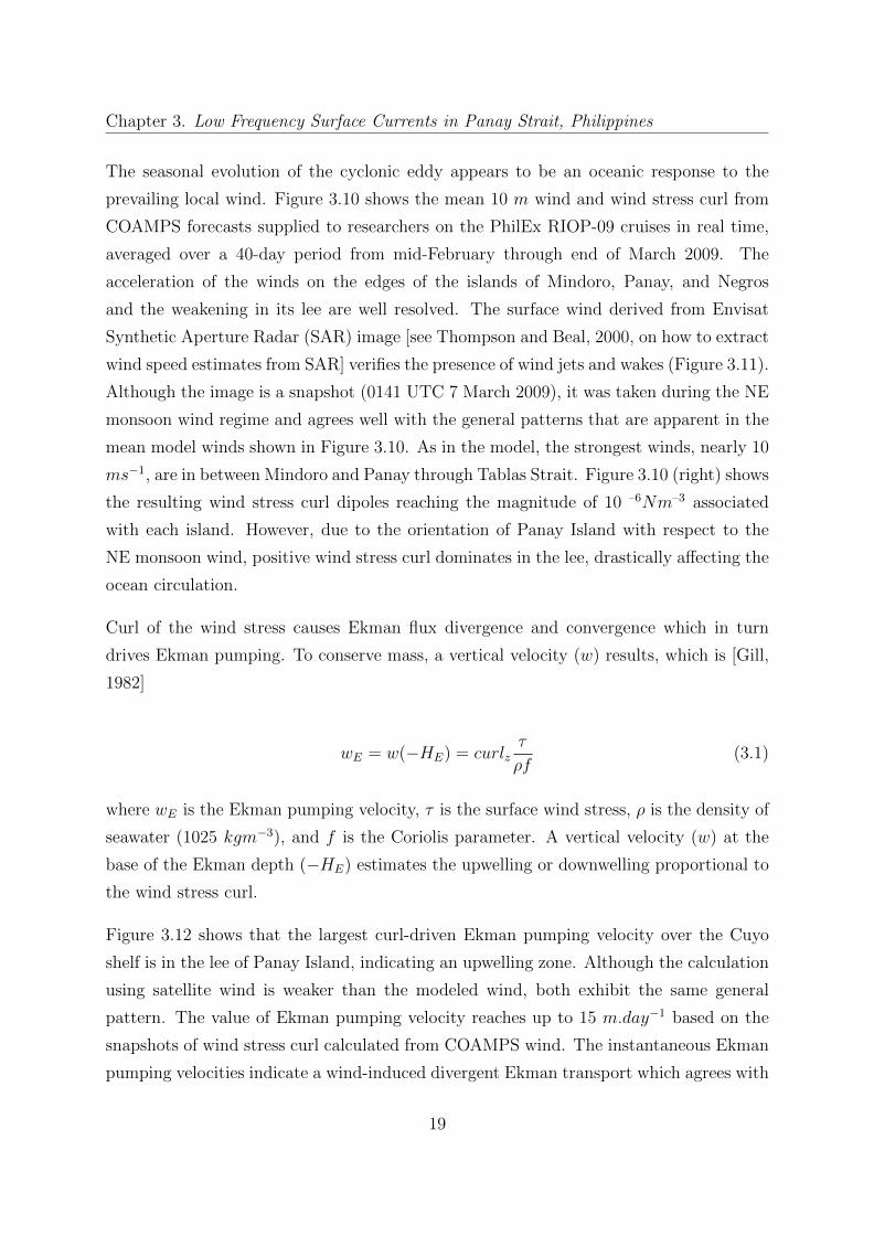
prevailing local wind. Figure 3.10 shows the mean 10 m wind and wind stress curl from
COAMPS forecasts supplied to researchers on the PhilEx RIOP-09 cruises in real time,
averaged over a 40-day period from mid-February through end of March 2009. The
acceleration of the winds on the edges of the islands of Mindoro, Panay, and Negros
and the weakening in its lee are well resolved. The surface wind derived from Envisat
Synthetic Aperture Radar (SAR) image [see Thompson and Beal, 2000, on how to extract
wind speed estimates from SAR] verifies the presence of wind jets and wakes (Figure 3.11).
Although the image is a snapshot (0141 UTC 7 March 2009), it was taken during the NE
monsoon wind regime and agrees well with the general patterns that are apparent in the
mean model winds shown in Figure 3.10. As in the model, the strongest winds, nearly 10
ms−1, are in between Mindoro and Panay through Tablas Strait. Figure 3.10 (right) shows
the resulting wind stress curl dipoles reaching the magnitude of 10 –6Nm–3 associated
with each island. However, due to the orientation of Panay Island with respect to the
NE monsoon wind, positive wind stress curl dominates in the lee, drastically affecting the
ocean circulation.
Curl of the wind stress causes Ekman flux divergence and convergence which in turn
drives Ekman pumping. To conserve mass, a vertical velocity (w) results, which is [Gill,
1982]
wE = w(−HE) = curlzτ
ρf(3.1)
where wE is the Ekman pumping velocity, τ is the surface wind stress, ρ is the density of
seawater (1025 kgm−3), and f is the Coriolis parameter. A vertical velocity (w) at the
base of the Ekman depth (−HE) estimates the upwelling or downwelling proportional to
the wind stress curl.
Figure 3.12 shows that the largest curl-driven Ekman pumping velocity over the Cuyo
shelf is in the lee of Panay Island, indicating an upwelling zone. Although the calculation
using satellite wind is weaker than the modeled wind, both exhibit the same general
pattern. The value of Ekman pumping velocity reaches up to 15 m.day−1 based on the
snapshots of wind stress curl calculated from COAMPS wind. The instantaneous Ekman
pumping velocities indicate a wind-induced divergent Ekman transport which agrees with
19

Chapter 3. Low Frequency Surface Currents in Panay Strait, Philippines
the mean divergence calculated from HFDR in the lee of the island during the same time
period (Figure 3.13). As a result of surface divergence, the thermocline is lifted and
the water column beneath is stretched, forming the Panay Dome. Figure 3.14 shows
the mean profile of (top) temperature and (middle) density from the hydrographic cross-
shore sections. The doming of isotherms and isopycnals corresponds well with the return
flow in the near-surface along-shore current from the shipboard ADCP, indicating the
center of the eddy. The excursion of the isolines reaches around 50 m. In the current
profile (Figure 3.14, bottom), the along-shore return flow reaches a depth of about 130
m, indicating the depth of the eddy. Velocities at the surface reached mean values of 50
cms−1. The flow structure is nearly depth-independent over the shallow shelf, whereas a
strong southward flow below 150 m is evident at the deep channel in the strait. Sprintall
et al. [2012] observed similar southward flows as extraordinarily strong pulses that begin
at intermediate depth in the Fall transition and shoal toward the sub-thermocline during
the NE monsoon found both in Mindoro and Panay Straits ADCP moorings. These
southward flows are strongly correlated with the changes in the South China Sea large-
scale circulation and remote wind forcing off Vietnam [Sprintall et al., 2012] .
The uplift in the thermocline sets up a horizontal pressure gradient, which consequently
spins up the geostrophic cyclonic eddy. The eddy formation is evident in the mean
vorticity overlaid by the surface current from HFDR, in which the center coincides with
the location of largest Ekman pumping and the doming (Figure 3.15).
If the divergence is entirely wind-driven and confined within the Ekman depth, divergence
should be proportional to the Ekman pumping velocity at the base of the Ekman layer.
That is
δ = ∇h.uh =wEHE
(3.2)
where δ = ∇h.uh is the divergence, subscripts h, denote horizontal components, and wE,
is the Ekman pumping velocity at constant Ekman depth, HE=32 m determined as the
best fit between the integrals of Ekman pumping velocity and divergence calculated by
Equation ?? and Equation ??, respectively.
Figure 3.16 shows the correlation between (top) divergence and Ekman pumping velocity
and between (bottom) vorticity and Ekman pumping velocity averaged over a specified
20

Chapter 3. Low Frequency Surface Currents in Panay Strait, Philippines
region (box in Figure 3.13 and Figure 3.15). All of the terms have been normalized by
f in order to facilitate comparison. The divergence and vorticity are significantly linked
together to Ekman pumping velocity, with correlation coefficient of R=0.50 and R=0.67
and RMS differences of 0.03 and 0.18, respectively.
3.3.4 Dynamical analysis of the cyclonic eddy
Vorticity input to the ocean from the overlying wind stress curl appears responsible for
the cyclonic eddy generation and evolution during the NE monsoon. By estimating the
surface vorticity balance of the low frequency surface current, wind contribution to the
generation and evolution of the vortex was assessed by
Dζ
Dt= −(f + ζ)δ − νβ +R (3.3)
where DζDt
= ∂ζ∂t
+u·∇ζ is the rate of change of vorticity following the fluid motion, (f+ζ)δ
is the vortex stretching, νβ is the Beta-effect term, where ν is the meridional velocity and
β is the meridional spatial derivative of f , and R is the residual term, assumed to be due
to friction and unresolved noises. Vorticity changes associated with sloping topography
was neglected.
Assuming that the momentum flux from the surface is due to wind stress, its contribution
to R is:
Rw =1
ρHE
curlzτ (3.4)
where ρ = 1025kgm−3 is the density of seawater, HE is the Ekman depth, and curlzτ is
the wind stress curl computed from QuikSCAT gridded daily wind.
Figure 3.17 (top) shows the temporal variation of each term in the vorticity balance
equation averaged over the same box in Figure 3.13 and Figure 3.15. Note that the β
term is magnified by a factor of 10 to show the trend. The evolution of the vorticity
within the vortex core was generally dominated by frictional processes, R, which drives
the formation of cyclonic vorticity from mid-November until mid-April. Observe, however
21
Chapter 3. Low Frequency Surface Currents in Panay Strait, Philippines
a significant R lag of about 10 days during NE monsoon, specifically during strengthening
of the cyclonic eddy during Dec.08, Feb.09 and Apr.09. Rw from QuikSCAT compares
well with the R from the HFDR observations, suggesting that the frictional forcing R is
induced dominantly by the wind stress curl driving the cyclonic vorticity growth after a
time lag of about 10 days (Figure 3.17, bottom).
Another interesting finding involves the β term. Recall the westward considerable shift
in the center of the eddy (Figure 3.7) during the waning NE monsoon. Figure 3.17 shows
that the shift coincides with an increasing β, though an order of magnitude less than
the other terms. We speculate that the β term causes the cyclonic eddy to propagate
westward in the manner of a Rossby wave.
Figure 3.18 and Figure 3.19 show the spatial distribution on 6 different days of each
term of the vorticity balance taken within the RIOP-09 period. If the Lagrangian rate
of change of vorticity is caused by frictional forcing, their spatial distribution should be
comparable. But since there is a considerable time lag between the two terms (Figure
3.17), disparity on their spatial variability notably exist.
3.3.4.1 Time lag between the wind forcing and the ocean response
To clarify the relationship between the cyclonic eddy formation processes and the wind
stress curl forcing (correlation shown in Figure 3.16), temporal variability of divergence,
δ, and relative vorticity, ζ, were plotted against the Ekman pumping velocity, wE
HE, pro-
portional to wind stress curl (Figure 3.20). Since a higher correlation exists between
divergence and the Ekman pumping velocity (Figure 3.16, top), Figure 3.20 (top) specifi-
cally shows that it occurs during strong and persistent NE monsoon winds although peaks
and dips occur due to the shifts of the eddy. In contrast, vorticity increases quickly with
progressing NE monsoon winds resulting in a relatively higher RMS=0.18 compared to
divergence with RMS=0.03. The Ekman pumping velocity is positive during October
when the NE monsoon prevail however, the response of the ocean to changes in the wind
stress curl is not instantaneous. The cyclonic vortex first appears as a closed circulation
in the low frequency current field only in mid-November indicated by positive vorticity
(0.05f) and attained its maximum in February 2009 (0.61f).
22

Chapter 3. Low Frequency Surface Currents in Panay Strait, Philippines
To further examine the time lag response of cyclonic eddy generation, the temporal
variation of thermocline depth anomaly is compared with the time integrals of the Ekman
pumping velocity and divergence. The best fit between the two terms was found at Ekman
depth, HE=32m and used as constant for all calculations.
The time integrals of the Ekman pumping velocity and divergence from a reference time
(July 28, 2008) represent their cumulative effect on the vorticity evolution, provided that
internal and external drags are neglected. Thermocline depth anomaly on the other hand
is proportional to vorticity, assuming a geostrophic balance in a 1.5 layer reduced gravity
model,
fu = −g′∂h∂y
−fv = −g′∂h∂x
(3.5)
where x and y are the conventional Cartesian coordinates, u and v the horizontal com-
ponents of velocity, f the Coriolis parameter, g′ = g∇ρρb
the reduced gravity (g is gravity
= 9.8 ms−2, ρb is the density at the motionless bottom layer, and ∇ρ is the density dif-
ference between the active top and motionless bottom layer, and h(x, y) the thermocline
depth anomaly.
Equations 3.7 were differentiated to obtain the relative vorticity and after some arranging,
yields:
f(∂v
∂x− ∂u
∂y) = −g′∇2h (3.6)
ζ =−g′∇2h
f(3.7)
The cyclonic eddy is assumed to be radially symmetric with sea surface height (h) per-
turbation at radial distance, r from the center of the eddy that has a Gaussian structure
of the form:
23
Chapter 3. Low Frequency Surface Currents in Panay Strait, Philippines
h(r) = h0 exp(− r2
L2) (3.8)
where h0 is the amplitude of the eddy, and L is the radius of the eddy. This height
function was substituted into Equation 3.5 to give:
h =ζfL2
g′(3.9)
L and g′ were estimated from the mean hydrographic cross-shore section while corre-
sponding vorticity, ζ was calculated from HFDR.
Figure 3.21 shows that the Ekman divergence is an instantaneous response to the positive
wind stress curl forcing. When NE monsoon prevails, after a quick transition period in
October (Figure 3.4), the integrated wind stress curl becomes positive. Consequently,
divergence occurs and increases rapidly along with the wind stress curl from mid-October
14, 2008 until mid-April 2009. After the transition period in April 2009, the wind stress
curl becomes very weak with no further increase in the time integral. In contrast, con-
vergence occurs during the SW monsoon period as the region is now dominated by the
northward PC jet resulting in relatively higher sea level and warmer temperature evi-
dent from the bottom pressure gauges measurements deployed during the same monsoon
regime in Pandan (Figure 3.22).
Correspondingly, a time lag response in the vorticity field occurs a month after mid-
November 2009 Figure 3.21) when it increases quickly, producing a mature and closed
cyclonic eddy circulation shown in Figure 3.6 (bottom). The current vorticity reaches its
maximum in January 2009, though HFDR data is missing but can be inferred from the
increasing values of vorticity and the strength of wind reaching its maximum during this
time of the year (Figure 3.4). After that initial period, ocean vorticity responds effectively
to fluctuating local wind magnitude and direction where peaks and dips correspond with
the strong and weak NE monsoon wind, respectively. A considerable decrease of vorticity
value in March 2009 indicate the westward shift of the center of the eddy in March 2009,
though the cumulative wind stress curl and divergence are still proportionally increasing.
This further support β term causing the cyclonic eddy to propagate westward.
24

Chapter 3. Low Frequency Surface Currents in Panay Strait, Philippines
3.4 Summary and Conclusion
High-resolution observations both in time and space of surface currents resolved the details
of the low-frequency mesoscale flow in Panay Strait. The surface circulation in the strait
has a distinctly seasonal cycle with the generation of a cyclonic eddy during the NE
monsoon, reinforcing the steady PC jet as its eastern limb.
The cyclonic eddy formation is the dynamic response to fluctuations in the monsoon
winds, specifically the variations of the wind jets blowing in between the islands of Min-
doro and Panay, generating the positive wind stress curl in the lee of Panay during the
NE monsoon. Based on observations and satellite-derived winds, wind curl field varia-
tions due to the changes in the strength and direction of the prevailing local wind play
an important role in the generation and evolution of the eddy, and variability of the PC
jet.
The region of positive wind stress curl causes Ekman flux divergence in the upper layer
which in turn drives Ekman pumping lifting the thermocline and stretching the water
column beneath, forming the Panay Dome. This results in horizontal pressure gradients,
which consequently generates a cyclonic eddy in geostrophic balance. The Panay Dome
is a subsurface upwelling, but to the west over the shallow Cuyo shelf, notable spreading
of isotherms and isopycnals indicate a vertically mixed water column, which destroys
the water column stratification. This therefore brings cooler, denser and nutrient-rich
waters into the euphotic zone leading to enhanced biological productivity over the region.
Satellite images confirmed cooler SST and enhanced chlorophyll concentration over the
Cuyo shelf, indicative of an active upwelling zone.
Evaluating all the terms of the surface vorticity balance equation suggests that the wind
stress curl via Ekman pumping mechanism provides the necessary input in the forma-
tion and evolution of the cyclonic eddy. The Beta-effect on the other hand may led to
propagation of the eddy westward.
In particular, the cumulative (time-integrated) effect of the wind stress curl plays a key
role on the generation of the cyclonic eddy, showing its robust mechanism to eddy kinetic
energy. Further, this study shows that unlike divergence, vorticity response to prevailing
25

Chapter 3. Low Frequency Surface Currents in Panay Strait, Philippines
wind stress curl is not instantaneous causing a time-lag, which may help towards under-
standing the physical development of coastal upwelling due to Ekman pumping in the lee
of the island.
26
Chapter 3. Low Frequency Surface Currents in Panay Strait, Philippines
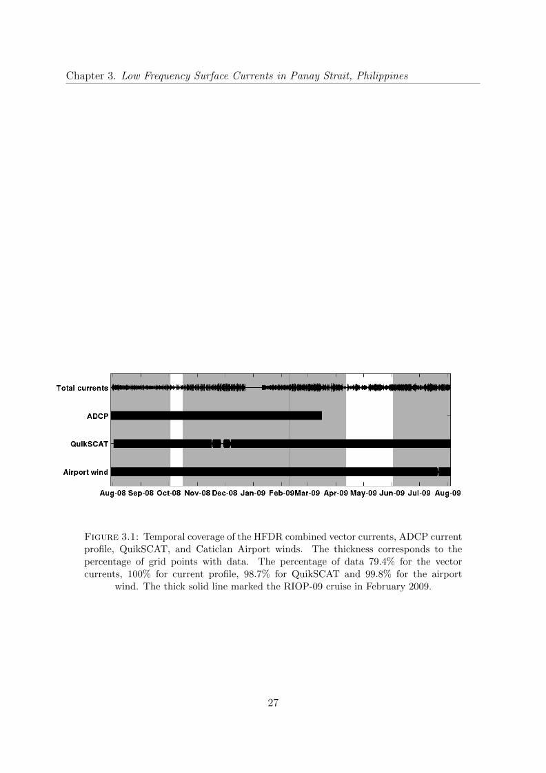
Figure 3.1: Temporal coverage of the HFDR combined vector currents, ADCP currentprofile, QuikSCAT, and Caticlan Airport winds. The thickness corresponds to thepercentage of grid points with data. The percentage of data 79.4% for the vectorcurrents, 100% for current profile, 98.7% for QuikSCAT and 99.8% for the airport
wind. The thick solid line marked the RIOP-09 cruise in February 2009.
27

Chapter 3. Low Frequency Surface Currents in Panay Strait, Philippines
Figure 3.2: Rotary power spectra of hourly (dark gray) and 6-day medianed (lightgray) HFDR data averaged over an area with more than 75% temporal coverage. Majortidal constituents (O1, K1, M2 and S1) and inertial frequency (f) are indicated on the
top x-axis.
28
Chapter 3. Low Frequency Surface Currents in Panay Strait, Philippines
Figure 3.3: Wind stress and curl from QuikSCAT at 25-km resolution, averaged overHFDR period during (top) NE monsoon (November-March) and (bottom) SW monsoon(May-September). Marked with star is the Caticlan airport where observed wind datawas obtained and correlated with the nearest QuikSCAT wind data shown in Figure
3.4.
29
Chapter 3. Low Frequency Surface Currents in Panay Strait, Philippines
Figure 3.4: Time-series wind vectors from nearby Caticlan airport and QuikSCATfrom the closest grid point. Correlations (R, the numbers in parentheses indicate the 5% statistical significant level) and root-mean-square differences (RMS diff) are indicated
in the top plot for zonal (U) and meridional (V) components.
30

Chapter 3. Low Frequency Surface Currents in Panay Strait, Philippines
Figure 3.5: Mean flow overlaid with speed contoured in cms−1 during (top) NEmonsoon and (bottom) SW monsoon. Three transects are marked accordingly along
which mean surface flow profiles are shown in Figure 3.6.
31

Chapter 3. Low Frequency Surface Currents in Panay Strait, Philippines
Figure 3.6: Time series profiles of (top) PC jet and (bottom) cyclonic eddy. Positive(negative) values indicate flow towards the north (south). The line color and type
corresponds to three transects in Figure 3.5.
32
Chapter 3. Low Frequency Surface Currents in Panay Strait, Philippines
Figure 3.7: Mean surface flow overlaying vorticity, ζ, normalized by f contours duringpeak (top, January 15–February 23, 2009) and waning (bottom, February 25-April 1,2009) NE monsoon. The arrows indicate the mean prevailing wind vectors from the
Caticlan airport.
33
Chapter 3. Low Frequency Surface Currents in Panay Strait, Philippines
Figure 3.8: Wind stress vectors overlaying the wind stress curl contours during peak(top, January 15–February 23, 2009) and waning (bottom, February 25-April 1, 2009)
NE monsoon from QuikSCAT.
34
Chapter 3. Low Frequency Surface Currents in Panay Strait, Philippines
Aug08 Sep08 Oct08 Nov08 Dec08 Jan09 Feb09 Mar09−60
−40
−20
0
20
40
60
TIME (MMMYY)
alo
ng
−s
ho
re c
urr
en
t [c
m/s
]
R = 0.76
depth (m)−120 −110 −100 −90 −80 −70 −60 −50
Figure 3.9: Time series along-shore current from moored ADCP (contoured) over-laid with along-shore surface current from the closest HFDR data (thick black line).Correlation (R) between HFDR and 50 m depth bin ADCP along-shore currents is
indicated.
35

Chapter 3. Low Frequency Surface Currents in Panay Strait, Philippines
Figure 3.10: The Coupled Ocean/Atmosphere Mesoscale Prediction System(COAMPS) left) 10 m mean wind, wind vectors plotted over wind speed contour (ms−1
and right) mean wind stress curl contour (Nm−3) from the 9 km computational gridsfor the Regional Intensive Observational Period, February to March 2009 (RIOP-09).
36
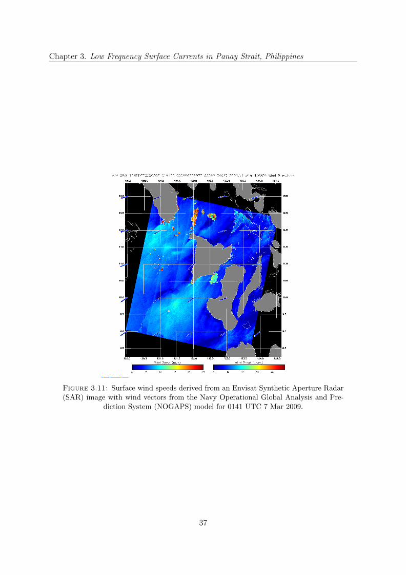
Chapter 3. Low Frequency Surface Currents in Panay Strait, Philippines
Figure 3.11: Surface wind speeds derived from an Envisat Synthetic Aperture Radar(SAR) image with wind vectors from the Navy Operational Global Analysis and Pre-
diction System (NOGAPS) model for 0141 UTC 7 Mar 2009.
37

Chapter 3. Low Frequency Surface Currents in Panay Strait, Philippines
Figure 3.12: Snapshots of surface current overlaid with contoured Ekman pumpingvelocity calculated from (left) QuikSCAT and (right) COAMPS wind. Wind vectors at
Caticlan airport (thick arrows) are also indicated.
38
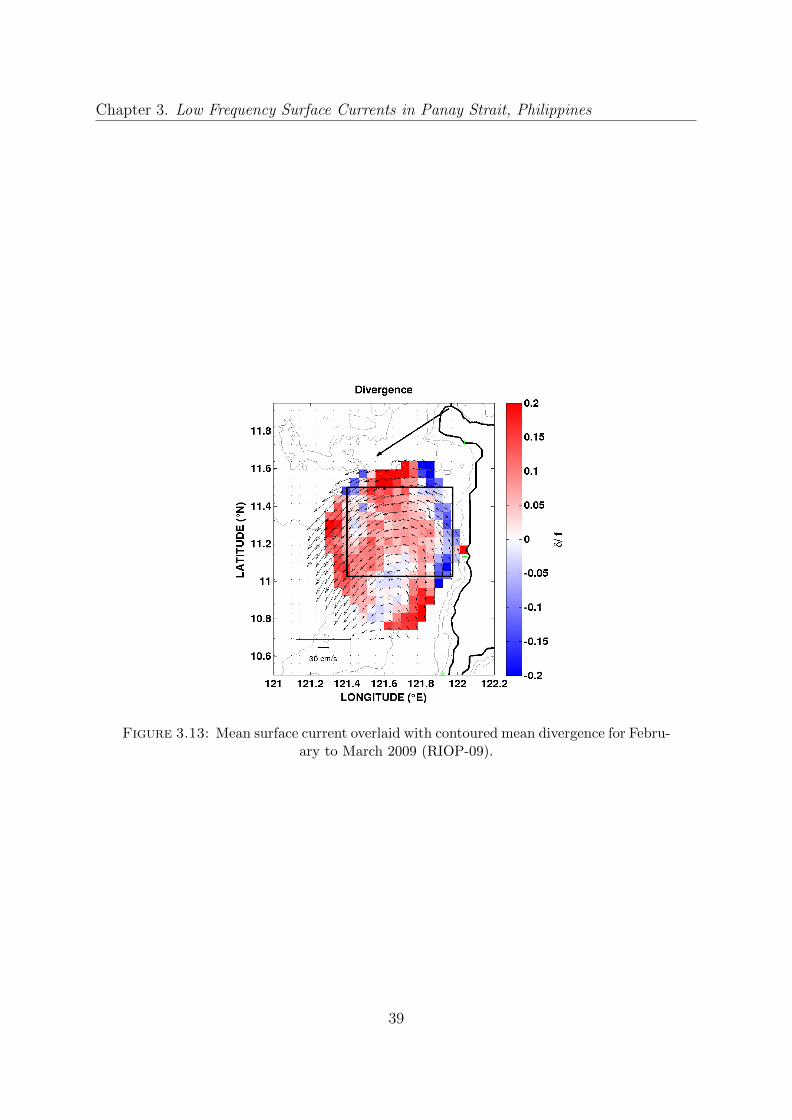
Chapter 3. Low Frequency Surface Currents in Panay Strait, Philippines
Figure 3.13: Mean surface current overlaid with contoured mean divergence for Febru-ary to March 2009 (RIOP-09).
39

Chapter 3. Low Frequency Surface Currents in Panay Strait, Philippines
Figure 3.14: Vertical transect of mean (top) temperature, (middle) density, and (bot-tom) along-shore flow from the shipboard ADCP across the Panay Strait during thehydrographic survey (February 8-9, 2009) shown in Figure 2.1. The mean near-surface
along-shore flow vectors are indicated above.
40

Chapter 3. Low Frequency Surface Currents in Panay Strait, Philippines
Figure 3.15: HFDR mean surface current overlaid with contoured mean vorticity forFebruary to March 2009 (RIOP-09).
41
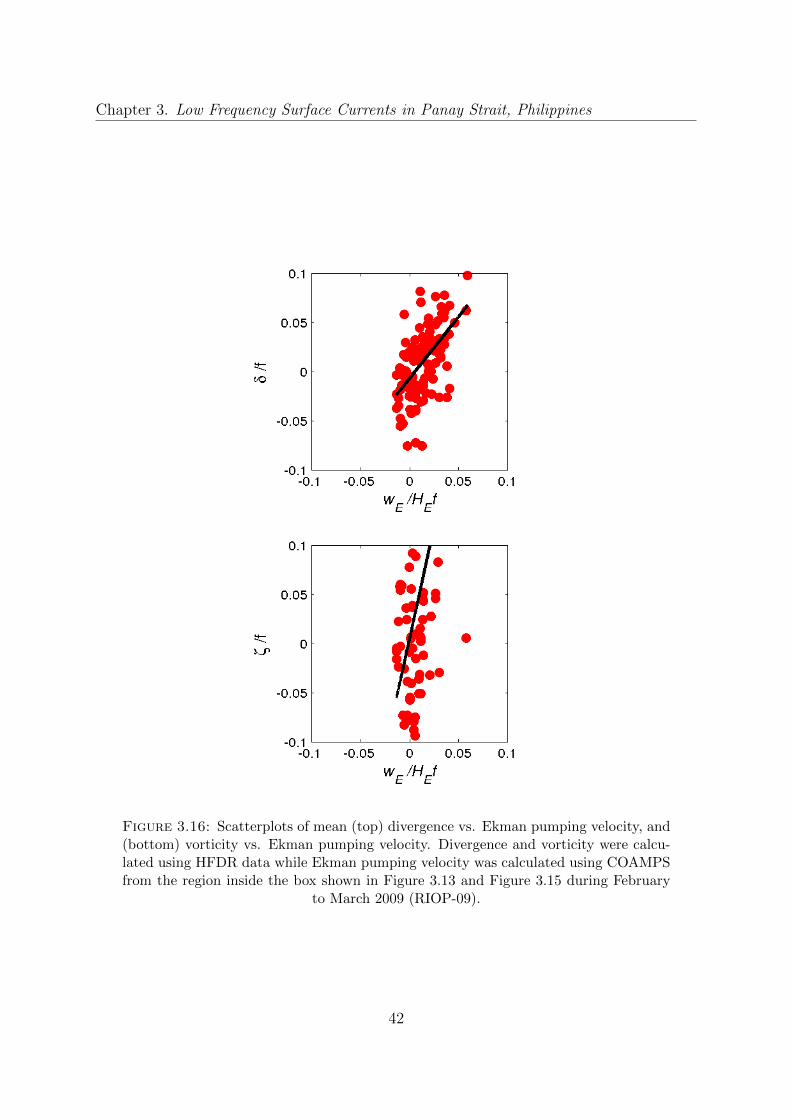
Chapter 3. Low Frequency Surface Currents in Panay Strait, Philippines
Figure 3.16: Scatterplots of mean (top) divergence vs. Ekman pumping velocity, and(bottom) vorticity vs. Ekman pumping velocity. Divergence and vorticity were calcu-lated using HFDR data while Ekman pumping velocity was calculated using COAMPSfrom the region inside the box shown in Figure 3.13 and Figure 3.15 during February
to March 2009 (RIOP-09).
42
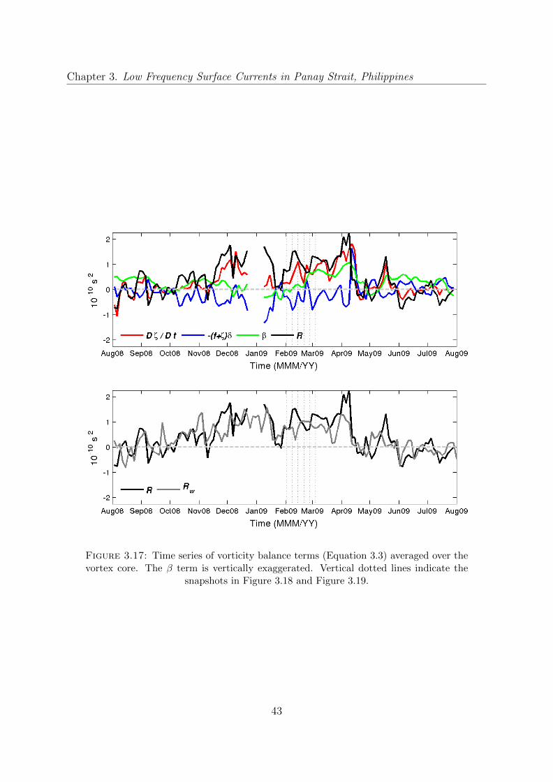
Chapter 3. Low Frequency Surface Currents in Panay Strait, Philippines
Figure 3.17: Time series of vorticity balance terms (Equation 3.3) averaged over thevortex core. The β term is vertically exaggerated. Vertical dotted lines indicate the
snapshots in Figure 3.18 and Figure 3.19.
43

Chapter 3. Low Frequency Surface Currents in Panay Strait, Philippines
Figure 3.18: Snapshots of the terms of the surface vorticity balance (Equation 3.3),overlaid with surface currents. From left to right, Lagrangian rate of change of vorticity,vortex stretching, residual, and Beta-effect terms. The times of snapshots are indicated
on the y-axis of the first column.
44

Chapter 3. Low Frequency Surface Currents in Panay Strait, Philippines
Figure 3.19: Snapshots of the terms of the surface vorticity balance (Equation 3.3),overlaid with surface currents. From left to right, Lagrangian rate of change of vorticity,vortex stretching, residual, and Beta-effect terms. The times of snapshots are indicated
on the y-axis of the first column.
45
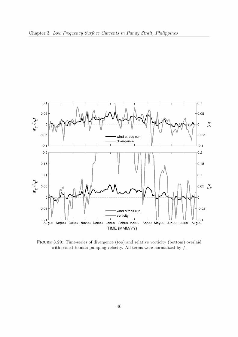
Chapter 3. Low Frequency Surface Currents in Panay Strait, Philippines
Figure 3.20: Time-series of divergence (top) and relative vorticity (bottom) overlaidwith scaled Ekman pumping velocity. All terms were normalized by f .
46

Chapter 3. Low Frequency Surface Currents in Panay Strait, Philippines
Figure 3.21: Vorticity overlaid with time integral of wind stress curl and divergenceconfined within the Ekman layer (HE = 32 m).
47

Chapter 3. Low Frequency Surface Currents in Panay Strait, Philippines
Figure 3.22: Time series (top) sea level and (bottom) temperature anomaly fromPandan and Tobias Fornier shallow pressure gauges.
48

Chapter 4
Coastal sea response to atmospheric
forcing in Panay Strait, Philippines
4.1 Abstract
High-resolution 10 m wind forecasts from the Coupled Ocean/Atmosphere Mesoscale Pre-
diction System (COAMPS) show the local atmospheric patterns in Panay Island, that
were not fully resolved by the gridded QuikSCAT wind data during the Regional Inten-
sive Observational Period cruises in February-March 2009 (RIOP-09) for the Philippine
Straits Dynamics Experiment (PhilEx). The Northeast (NE) monsoon is characterized by
distinct wind jets between islands and mountain gaps that generates an alternating band
of positive and negative wind stress curl to the right and left downwind of each island.
These bands are also observed in the Envisat Synthetic Aperture Radar (SAR) images.
The Panay coastal sea response includes formation of a cyclonic Panay Lee (PL) eddy, the
relatively smaller cyclonic Panay Tip (PT) eddy on the northwest flank of the island, and
the localized coastal upwelling in Pandan revealed by the sea level measurements from
the moored shallow pressure gauge and temperature from SBE37 CTD. Multiple sample
iterations with TRIAXUS and ADCP repeatedly map subregions covering the PL and
PT eddy which resolve tidal variability and low-frequency variability that represents the
seasonal response to monsoon winds. The observed features were confirmed by satellite
observations of sea surface temperature and chlorophyll concentration provided in near
real-time during the PhilEX cruise.
49
Chapter 4. Coastal sea response to atmospheric forcing in Panay Island, Philippines
4.2 Introduction
The Philippine Archipelago region is a complex array of islands and semi-enclosed seas
with interconnecting straits and sills. Atmospheric circulation is governed by the reversal
of the East Asian monsoon and the relatively steady Pacific trade winds. Circulation
within and around the Philippines is mainly influenced by a range of processes such
as tidal variations, seasonal reversal of the monsoon, sea level variations between West
Philippine Sea to the west and the western Pacific Ocean to the east, inter-annual vari-
ations such as El Nino Southern Oscillation, and episodic occurrence of monsoon surges
and tropical cyclones.
Within the island archipelago, however, finer scale variability both in the atmosphere
and the ocean are primarily controlled by island topography and morphology, which
adds complexity to the interisland circulation. In a one-way coupled atmosphere and
ocean simulation of the Philippine region, monsoon winds interacting with the volcanic
topography, lead to strong wind jets between islands and through gaps in the rugged
terrain [Pullen et al., 2008]. The model simulations show that steady monsoon winds
form stationary lee eddies, while monsoon surges frequently occurring during the winter
season trigger oceanic eddy formation and propagation depending on the orientation of
the winds in the lee of the islands. Another simulation shows the regional and local nature
of atmospheric patterns and the ocean response during RIOP-09 cruise [May et al., 2011].
It confirms that prominent, topographically generated wind jets in the gaps between the
islands, and the wakes downwind of the islands are persistent features during the NE
monsoon. Local details of the ocean response were revealed using fine-scale atmospheric
and ocean model grids while the presence of upwelled nutrient-rich water was supported
by elevated chlorophyll concentration in satellite imagery and in-situ measurements [May
et al., 2011].
The linkage between atmospheric dynamics and oceanic eddy characteristics was inferred
from high-resolution air-sea modelling [Pullen et al., 2008]. Though in reasonable agree-
ment with contemporaneous satellite and in-situ historical data, high spatial and temporal
resolution, in both observations and modeling are still needed to confirm.
In this study, coastal sea response to local atmospheric forcing is investigated using current
profiles from shipboard ADCP and CTD/fluorometer sections in conjunction with satellite
50
Chapter 4. Coastal sea response to atmospheric forcing in Panay Island, Philippines
observations of sea surface temperature and chlorophyll concentration. Along with in-situ
measurements during the RIOP-09, time series data of sea level from shallow pressure
gauge (SPG), temperature from SBE37 CTD collocated with SPG, and inferred surface
current from High Frequency Doppler Radar (HFDR) are used to investigate how the
influence of island topography on the local wind regime translates to sea level, surface
flows and hydrographic variability.
4.3 Methods
The Office of Naval Research (ONR)-sponsored Philippine Straits Dynamics Experiment
(PhilEx) Intensive Observational Period cruise was conducted focusing on the dynamically
narrow straits of the Philippines. This multi-disciplinary research cruise was held in
February 2009 (RIOP-09) under the NE monsoon regime on-board the R/V Melville
(Figure 4.1). Directed by real-time data support such as sea surface temperature, wind
speed and ocean color images, successive and multiple transects employing towed profiling
vehicle and hull-mounted shipboard 150 kHz ADCP provided the nearly synoptic views of
water column hydrography and velocity along the ship track. The hydrographic sections
were made by towing a TRIAXUS, an undulating vehicle equipped with physical and
optical sensors making quasi-synoptic, high-resolution, three-dimensional surveys of the
upper ocean [see Jones et al., 2011, on the TRIAXUS sampling approach]. TRIAXUS
maintained a vertical speed of 1 ms−1 while typically being towed at 7 knots, with along-
track horizontal resolution of 1 km or less, dependent on profile depth. TRIAXUS carried
two pairs of Sea-Bird temperature and conductivity sensors along with upward (1200
kHz) and downward (300 kHz)-looking RDI acoustic Doppler current profilers. Here
we used all the synoptic measurements obtained during the seven-day period between
February 8 and 15, 2009 by TRIAXUS focusing north of Panay Strait which include the
Thalweg section between Mindoro and Panay Island, the transect on the northwest (NW)
tip of Panay Island, and repeated sections over Pandan Bay to investigate the coastal sea
response to local wind forcing. Concurrent and subsequent along-track velocity profiles
and repeated sections over Pandan Bay (Figure 4.2) over a 24-hour span were used to
resolve the tidal variability within each survey pattern. Cruise data used for analysis
were depth profiles of velocity from the shipboard ADCP and conductivity, temperature
and chlorophyll concentration from CTD/fluorometer.
51
Chapter 4. Coastal sea response to atmospheric forcing in Panay Island, Philippines
In addition, the Naval Research Laboratory (NRL) supplied the real-time atmospheric
and oceanic forecasts for the cruises. This NRL coupled atmosphere-ocean model pro-
vides simultaneous high-resolution studies of both the meteorology and oceanography of
the region. The numerical simulations for the Philippines used the Coupled Ocean/At-
mosphere Mesoscale Prediction System (COAMPS), which consists of an atmospheric
model coupled with the Navy Coastal Ocean Model (NCOM) [see May et al., 2011, for
a more detailed description of the model]. Daily near-surface winds from COAMPS in 9
km resolution and from QuikSCAT in 25km resolution were analyzed to determine the
effects of the surface winds on the ocean features observed.
The vertical component of the wind stress curl was estimated from the COAMPS 10 m
wind stress fields.
(∇× τ).k = curlz(τ) =∂τy∂x− ∂τx
∂y(4.1)
τ is the 10 m wind stress, x and y are the east and north coordinates, respectively.
Time-series observations of sea surface current in Panay Strait (July 2008 – August 2009)
provided by HFDR in conjunction with sea level measurements from shallow pressure
gauges (October 2007 – April 2009) were used to examine modifications in the surface
flows and sea level in response to local wind forcing. The vector currents generated from
the radial component of the current from three HFDR sites located at Pandan, Laua-an,
and Tobias Fornier at the western coast of Panay Island undergo quality control prior
to the analysis (see Chapter 2 for more detailed description of the data processing). At
each, grid point, 75 % temporal coverage of over a year data were used.
The sea level data were obtained from shallow pressure gauges deployed approximately 5-
10 m depth just in front of the north HFDR site. Pressure is measured every ten minutes
by a Paroscientific quartz pressure sensor with an accuracy of 0.3 mb. Correction for the
static inverse barometer (IB) effect of fluctuations in atmospheric pressure on sea level
was disregarded since it was found to be far smaller (order of 10 −2 to 10 −1cm) than the
magnitudes of the sea level variability observed. In addition, surface temperature and
salinity were obtained from SBE37 CTDs collocated with the shallow pressure gauge.
52

Chapter 4. Coastal sea response to atmospheric forcing in Panay Island, Philippines
The tidal components in the time-series data were estimated by performing a harmonic
tidal analysis using T-Tide, an open source MATLAB toolbox as described by Pawlowicz
et al. [2002]. The tidal prediction time-series were obtained and compared with the
shipboard ADCP resolving the tidal variability within each survey pattern.
4.4 Results and Discussions
4.4.1 Cruise Observational data
4.4.1.1 Velocity field
The complexities of the flow of the Panay coastal waters were captured by HFDR and ship-
board ADCP that obtain high horizontal resolution of sub-mesoscale features. Though
the measurements were made in different temporal resolutions, both the mean and syn-
optic measurements show predominant surface flows composed of a cyclonic Panay lee
(PL) eddy, and a northward Panay coastal (PC) jet which flows along the coast, branches
out to the left forming the northern limb of the PL eddy and to the right flowing further
north, veers westward and retroflects to form the small cyclonic Panay tip (PT) eddy off
the promontory (Figure 4.3).
Two successive surveys in February 8-10, 2009 and February 11-15, 2009 focused on two
eddy formations at the lee and off the tip of Panay headland, generating synoptic maps
of the apparent flows (Figure 4.4A and B). Multiple sample iterations of each region were
performed over a 24-hour span, thus resolving tidal variability within each survey pattern.
The first survey focused on the PL eddy (Figure 4.4A). The near-surface velocities (with
maximum speed of 95 cms−1 over the shallow shelf show a strong shear centered near
11.25 ◦ N, 121.7 ◦ E indicating the core of the PL eddy. Its eastern limb, the strong
northward PC jet flows along the coast with subsequent flow separation as it encounters
the Batbatan Island. The left branch flows westward and shears forming the northern
limb of the PL eddy. The relatively weaker right branch flows north close to the coast. An
offshore flow is evident as it passes across the mountain gap, then intensifies northward
and veers westward as it encounters an abrupt change in the angle of the coastline. It
53
Chapter 4. Coastal sea response to atmospheric forcing in Panay Island, Philippines
then slightly shears past the tip of the Panay headland, indicating the formation of the
PT eddy.
Figure 4.4B shows a detailed survey of the PT eddy. The measurements start a little
further north, which barely captures the shear at 11.3 ◦ N indicating the core of the PL
eddy. However, the survey reveals an energetic cyclonic eddy with maximum speed of
about 100 cms−1. Two sections that traverse from the lee of Panay to the tip of the
headland clearly show the PL eddy extending further north near 11.64◦N , defined by the
strong northwestward PC jet. The strong shears are now clearly visible with subsequent
return flow in the surveys close to the NE corner of Panay over Pandan Bay, distinctly
indicating a smaller coastal eddy structure.
The two surveys span the seven-day period with one-day sampling (February 10-11,
2009)in Tablas Strait in between, which was designed to obtain measurements across the
strait, separating the islands of Mindoro and Panay. The combination of both monsoon-
driven and tidally-driven currents predominate in the study area. The first survey was
conducted during spring tide and relatively stronger winds, in contrast to the second
survey during neap tide and weaker winds. Several locations were occupied during the
survey, obtaining one-time measurements of the velocity structure during different wind
conditions. The multiple cross-shore surveys covering the eddies over a 24-hour span
on the other hand, give an opportunity to resolve current structure during varied tidal
conditions.
Panay Lee (PL) Eddy Panay Strait sea level has semidiurnal tidal cycles based on
measurements from the shallow pressure gauge moored at Pandan, Antique (Figure 4.5).
During the 24-hour successive cross-shore survey of Panay Strait, mixed tidal variability
at K1 (23.9 hours), O1 (25.8 hours) and M2 (12.4 hours) periods predominated (Figure
4.6A). The survey was conducted during the NE monsoon regime and spring tide. The
sequence of synoptic current vectors from different depths obtained through the tidal
cycle has significantly different flow structures (Figure 4.6B and C). During flood tide
(left panels), the near-surface current from the 12 m depth bin was intensified over the
shelf with maximum speed of 94.5 cms−1, while during the ebb tide (right panels), the
intensified flow (60 cms−1) was at about 200 m depth over the channel. This is consistent
with the high percentage of variance explained by the four major tidal constituents (O1,
54
Chapter 4. Coastal sea response to atmospheric forcing in Panay Island, Philippines
K1, M2 and S2) over the shallow shelf from the HFDR inferred surface currents and in
the distinct layer centered at about 250 m from the moored ADCP (see Chapter 5).
Figure 4.7A to D shows the full velocity profiles during the flood tide (left panels) and
ebb tide (right panels), providing a comparison of the water-column current structures
during different tidal conditions under the NE monsoon regime. Generally, an enhanced
current flow with strong shear in the upper (0-130 m) layer is clearly visible indicating the
northward PC jet (in red) and the southward flow (in blue) comprising the wind-driven
cyclonic PL eddy. Over the deep channel below the PC jet is a southward flow (in blue)
with core at depth of about 200 m. A considerable modification of these dominant flows
are noticeable over the tidal cycle, with a strengthening of current near the surface during
flood tide (Figure 4.7 A and C), and at subsurface (130 m) during the ebb tide (Figure
4.7 B and D).
This sampling period coincides with relatively stronger wind as shown in Figure 4.4 from
observations at Caticlan airport. The combined influence of wind and relatively strong
tides generate an intensified flow reaching the shallow bottom of the Cuyo Shelf (Figure
4.7A and B). While a more wind-driven surface flow is clearly visible during weaker tides
in response to the more easterly prevailing wind (seen in Figure 4.4A) which considerably
moved the shear region to the west indicating a shift of the PL eddy westward (Figure
4.7D).
Panay Tip (PT) Eddy Figure 4.8A shows that semidiurnal tidal variability domi-
nates sea level during the intensive survey north of the PT eddy in February 13-14, 2009
(Figure 4.5A). The sequence of synoptic near-surface current maps from the 12 m depth
bin obtained through the tidal cycle, as colored accordingly, are shown in panels B to C.
Starting at low tide (Figure 4.8B), a transect traversing up to the tip of Panay (in blue)
shows a strong wind-driven northwestward flow with maximum speed of 61 cms−1 and a
strong shear near the tip of the headland, an indication of a PT eddy in that area. At
flood tide (in purple), a strong northwestward flow near the tip of the headland is evident
with shift of the eddy to the east toward the coast as the tidal height attains a maxima on
February 13, 2006 at 1600-hour period. During the subsequent ebb tide (Figure 4.8C, top
left), the flow near the tip of the headland veers southwestward and consequently shifts
the eddy away from the coast. This oscillation in the current pattern goes on through the
tidal cycle. The eastward current towards the coast during flood tide and the westward
55
Chapter 4. Coastal sea response to atmospheric forcing in Panay Island, Philippines
current away from the coast during the ebb tide are consistent with the tidal current
extracted from the surface current inferred from the HFDR, despite the fact that regions
close to the coast were disregarded due to Geometric Dilution of Precision (GDOP).
4.4.1.2 RIOP-09 Cruise Hydrographic data
The TRIAXUS survey near the Panay tip (Figure 4.9) did not coincide with shipboard
ADCP. The survey observations started during the slack water at low tide and continued
to the flood and ebb tide period as colored accordingly in the sea level measurements in
Figure 4.9A. Distributions of temperature, salinity and density show doming of isolines
indicating the PT eddy structure captured near the headland, specifically during the
1200-1300 hour survey and during 1700-1800-hour survey. The doming is associated with
high chlorophyll concentration with stronger signal at the dome (1200-1300-hour) during
flood tide when the current velocity is stronger and the eddy reached deeper (about 100
m) in the water column (Figure 4.9 E)).
Thalweg Distributions A Thalweg section between Mindoro and the Panay straits
spanned a 15-hour period during the ebb tide covering a distance from 0 to 87 km (08-
Feb-2009 14:01:00 to 08-Feb-2009 21:00:00) and the flood tide at the rest of the transect
(08-Feb-2009 21:00:00 to 09-Feb-2009 05:01:35) (Figure 4.10). An examination of this
section directly over the channel and across gap between islands provides insight into
tidally and wind-driven processes.
During ebb tide, an intrusion of warm and fresh water from Mindoro in the upper 50
m is clearly visible particularly in the salinity profile (Figure 4.10 C, bottom) reaching
about 90 km south of the transect. A significant change however is notable at 40 km
past the island of Mindoro, eroding the minimum salinity signature concurrent with the
intensified southwestward surface current and a 70 m depth core of strong flow toward
the Mindoro Strait from the current profile (Figure 4.10 B). This is accompanied further
by outcropping of isotherms and isopycnals indicating an enhanced vertical mixing due
to intensified northeasterly wind in the gap between the islands. A relatively weak and
directionally variable surface current in the lee of the islands of Caluya and Sibay notably
formed a weak stratification but as flood tide arrives and the survey track crosses the
channel towards Panay Island, a stronger outcropping of isolines occur at about 100 km
56

Chapter 4. Coastal sea response to atmospheric forcing in Panay Island, Philippines
followed by a doming which uplift the isotherms and isohalines by 50 m from 100 m
depth. These outcropping of isolines in between islands centered at 70 km and 110
m is due to the wind and tidally-driven flow within these channels. Associated with it
is an elevated chlorophyll concentration in the upper 80 m of the water column, more
so in the section near south Mindoro where two principal rivers, namely Busuanga and
Lumintao, drain that may supply nutrients, supporting higher biological productivity in
the region. At 120-160 km, the resulting doming of the isolines is due to the PL cyclonic
eddy captured during the survey (Figure 4.10 A).
4.4.1.3 T/S Distributions
The direct connection of the Philippine internal seas to the western Pacific are through
the shallow San Bernardino Strait, with a sill depth of 92 m, Surigao Strait, with sill
depth of 58 m and the deeper Luzon Strait with sill depth of 2200 m. The data from the
western Pacific adjacent to San Bernardino Strait displayed a pronounced salinity maxima
(s-max) in the 50 to 250 m depth range, 15 to 26 ◦C temperature interval (Figure 4.11
C) that marks North Pacific Subtropical Mode Water [Hanawa and Talley, 2001].
In comparison, the temperature/salinity (T/S) profile within the Panay Strait region
(Figure 4.11 B) shows a weak signal of the North Pacific Subtropical s-max while enter-
ing into the confines of the Mindoro and Tablas Straits. At the surface, there are two
characteristic water masses, the salinity minimum (s-min) brought by lighter freshwater
drained by two principal rivers south of Occidental Mindoro, and the relatively colder
and saltier water mass due to shallow upwelling/doming that generates PL and PT ed-
dies and the intense turbulent mixing in gaps between islands. Since the s-min layer lies
well above the sill depth in Mindoro Strait, intrusion of this water mass was captured as
subsurface flow into the Panay Strait and further south to the Sulu Sea Basin.
At the Mindoro Strait section of the Thalweg, the s-max core is greatly weakened, shown
as slight T/S bend near 25.5 ◦C at 70 m and near 24 ◦C at 110 m in the Tablas Strait.
A deeper s-max in the 150 m near 16 ◦C however are depicted in all survey tracks,
indicating access of Pacific water via the Mindoro and Tablas straits through the Verde
Island Passage.
57
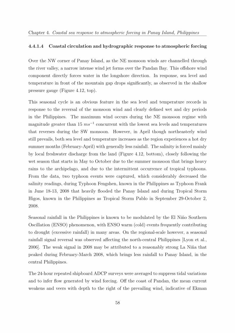
Chapter 4. Coastal sea response to atmospheric forcing in Panay Island, Philippines
4.4.1.4 Coastal circulation and hydrographic response to atmospheric forcing
Over the NW corner of Panay Island, as the NE monsoon winds are channelled through
the river valley, a narrow intense wind jet forms over the Pandan Bay. This offshore wind
component directly forces water in the longshore direction. In response, sea level and
temperature in front of the mountain gap drops significantly, as observed in the shallow
pressure gauge (Figure 4.12, top).
This seasonal cycle is an obvious feature in the sea level and temperature records in
response to the reversal of the monsoon wind and clearly defined wet and dry periods
in the Philippines. The maximum wind occurs during the NE monsoon regime with
magnitude greater than 15 ms−1 concurrent with the lowest sea levels and temperatures
that reverses during the SW monsoon. However, in April though northeasterly wind
still prevails, both sea level and temperature increases as the region experiences a hot dry
summer months (February-April) with generally less rainfall. The salinity is forced mainly
by local freshwater discharge from the land (Figure 4.12, bottom), closely following the
wet season that starts in May to October due to the summer monsoon that brings heavy
rains to the archipelago, and due to the intermittent occurrence of tropical typhoons.
From the data, two typhoon events were captured, which considerably decreased the
salinity readings, during Typhoon Fengshen, known in the Philippines as Typhoon Frank
in June 18-13, 2008 that heavily flooded the Panay Island and during Tropical Storm
Higos, known in the Philippines as Tropical Storm Pablo in September 29-October 2,
2008.
Seasonal rainfall in the Philippines is known to be modulated by the El Nino Southern
Oscillation (ENSO) phenomenon, with ENSO warm (cold) events frequently contributing
to drought (excessive rainfall) in many areas. On the regional-scale however, a seasonal
rainfall signal reversal was observed affecting the north-central Philippines [Lyon et al.,
2006]. The weak signal in 2008 may be attributed to a reasonably strong La Nina that
peaked during February-March 2008, which brings less rainfall to Panay Island, in the
central Philippines.
The 24-hour repeated shipboard ADCP surveys were averaged to suppress tidal variations
and to infer flow generated by wind forcing. Off the coast of Pandan, the mean current
weakens and veers with depth to the right of the prevailing wind, indicative of Ekman
58

Chapter 4. Coastal sea response to atmospheric forcing in Panay Island, Philippines
dynamics (Figure 4.13A and B). Recall that Ekman layer velocities get more and more
perpendicular with the direction of the wind as the water depth reaches the bottom of the
Ekman depth. This Ekman transport is seen to reach about 50 m shown as northward
flow (Figure 4.13 B, red contour) with about 15 cms−1 speed (Figure 4.13 A, with contour
line), except at the southwest corner of the survey tracks where a southward retroflection
(blue contour at 30 m distance) indicates the structure of PT eddy. This current is
comparable with the Ekman drift calculated using the wind stress from COAMPS (not
shown) estimated by:
ue =τ y
fρHe
ve = − τx
fρHe
(4.2)
where ue and ve are zonal and meridional components, τx and τ y are zonal and meridional
surface wind stress, ρ = 1025kgm3 is water density and He = 50m is the Ekman layer
thickness.
A smaller band of positive wind stress curl at the northern tip of Panay (Figure 3.10
in Chapter 3) suggests Ekman pumping as the mechanism that generates the cyclonic
PT eddy. And since the region is mainly driven by monsoon reversing winds, it can be
considered as persistent and permanent feature similar to the PL eddy during the NE
monsoon regime.
4.4.1.5 Satellite Imagery
MODIS Sea Surface Temperature (SST) 7-day composite images for February 7 to 13,
2009 show cooler SST (Figure 4.14, left) collocated with the intensified winds over Tablas
Strait in between Mindoro and Panay and at the northwest tip of Panay that blows di-
rectly offshore, and warmer SST in the calm lee of Panay Island. In response to intensified
winds, mean GHRSST SST data shows a remarkable tongue of cooler water advected by
PL eddy over the Cuyo shelf .
59

Chapter 4. Coastal sea response to atmospheric forcing in Panay Island, Philippines
The mean profile of water properties from repeated cross-shore surveys near the center of
PL eddy shows doming of the isoline contours indicating upwelling of cooler and saltier
waters to about 40 m (based on σt = 22.5) excursion near the core (Figure 4.15). This
eddy feature was associated with a subsurface chlorophyll maxima (0.045 mg/m3) found
well above the thermocline, with the mixed layer concentration near the core two times
greater than the periphery of the eddy.
The satellite imagery provided real time support to the cruise and confirmed the cooling
and enhanced chlorophyll concentration over the Cuyo shelf region (Figure 4.16). The
seasonal and spatial variations of chlorophyll concentrations, SST, wind fields and wind-
induced Ekman pumping over this region were apparent in the 7-year monthly mean
remote sensing measurements from October 1997 to December 2004 [Wang et al., 2006].
The seasonal variation of chlorophyll concentrations and SST distributions were asso-
ciated with the seasonally reversing monsoon winds. The winter (December-February)
phytoplankton blooming and the tongue of the cold waters were correlated to the vertical
upwelling of cold and nutrient-rich waters drawn by the NE wind. The center of the
blooms and location of cold tongues in the gaps between Mindoro and Panay coincide
with the maximum of the wind speeds and the Ekman pumping velocities, consistent
with the observational results in this study.
Previous studies during the transition to the NE monsoon (October) identified Cuyo
Shelf as having abundant fish larvae and inferred it to be a major source of larvae to the
Sulu Sea. This is an important information needed to establish an ecologically functional
network of Marine Protected Areas (MPA) over the region [Campos et al., 2008].
The survey tracks measuring the water property distribution of the PT eddy did not
perform multiple iterations along with the shipboard ADCP thus no mean profile was
computed. However, a synoptic profile of temperature, salinity and density clearly re-
vealed a doming of isolines of 50-55 m excursion near the core indicating the cyclonic
PT eddy feature (Figure 4.9). This clearly altered the vertical phytoplankton biomass
distribution as indicated by increased chlorophyll concentration near the core/doming.
60

Chapter 4. Coastal sea response to atmospheric forcing in Panay Island, Philippines
4.5 Summary and Conclusion
In this paper, the response of the coastal ocean to forcing by tides and winds were
investigated. Measurements in Panay Strait captured the predominant surface flows
composed of the cyclonic Panay lee (PL) eddy, a northward Panay coastal (PC) jet
which flowed along the coast, then branched and veered westward while another branch
flowed further up north, retroflects and forms the small cyclonic Panay tip (PT) eddy off
the promontory. The narrow intense wind jet through the mountain gap blowing directly
offshore over Pandan Bay generated an Ekman current, reinforcing a branch of the Panay
jet which comprises the eastern limb of the PT eddy.
Panay Strait has a semidiurnal tidal cycle based on measurements from the moored
shallow pressure gauge. Repeatedly mapping subregions covering the PL and PT eddy
resolved tidal variability. During flood tide, the PL eddy has an intensified near-surface
flow over the shallow Cuyo shelf while at about 200 m over the deep channel during ebb
tide. The spring tides generate an intensified flow and enhanced mixing over the shelf.
Tidal oscillation is evident for the PT eddy. It shifts eastward towards the coast during
the flood tide and westward away from the coast during the ebb tide. A considerable
deepening of the PT eddy is also evident reaching the depth of about 100 m during flood
tide and only about 50 m during ebb tide.
The PL eddy is significantly bigger, about 100 km, than the PT eddy, less than 15 km in
diameter. Since the PL eddy was within the HFDR coverage, details of its generation and
evolution were well examined and discussed using inferred surface currents in high spatial
and temporal resolution during the NE monsoon. Due to Geometric Dilution of Precision
(GDOP) (see Chapter 3), the PT eddy was outside the reduced HFDR coverage thus the
formation mechanism was inferred from in-situ shipboard measurements and real-time
COAMPS ocean forecast provided during RIOP-09 cruise. Based on the observations
and model data, formation and evolution of the PT eddy was inferred to be similar to
the PL eddy, that is due to positive wind stress curl that may induce a divergent surface
flow which in turn uplifts the thermocline and creates a pressure gradient that spins-up
this geostrophic eddy. A branch of Panay coastal jet as its eastern limb was reinforced
by the Ekman current driven by the wind jet through the mountain gap blowing directly
61

Chapter 4. Coastal sea response to atmospheric forcing in Panay Island, Philippines
offshore over Pandan Bay. Since both are generated during the NE monsoon they tend
to be permanent features that persist during this wind regime.
62
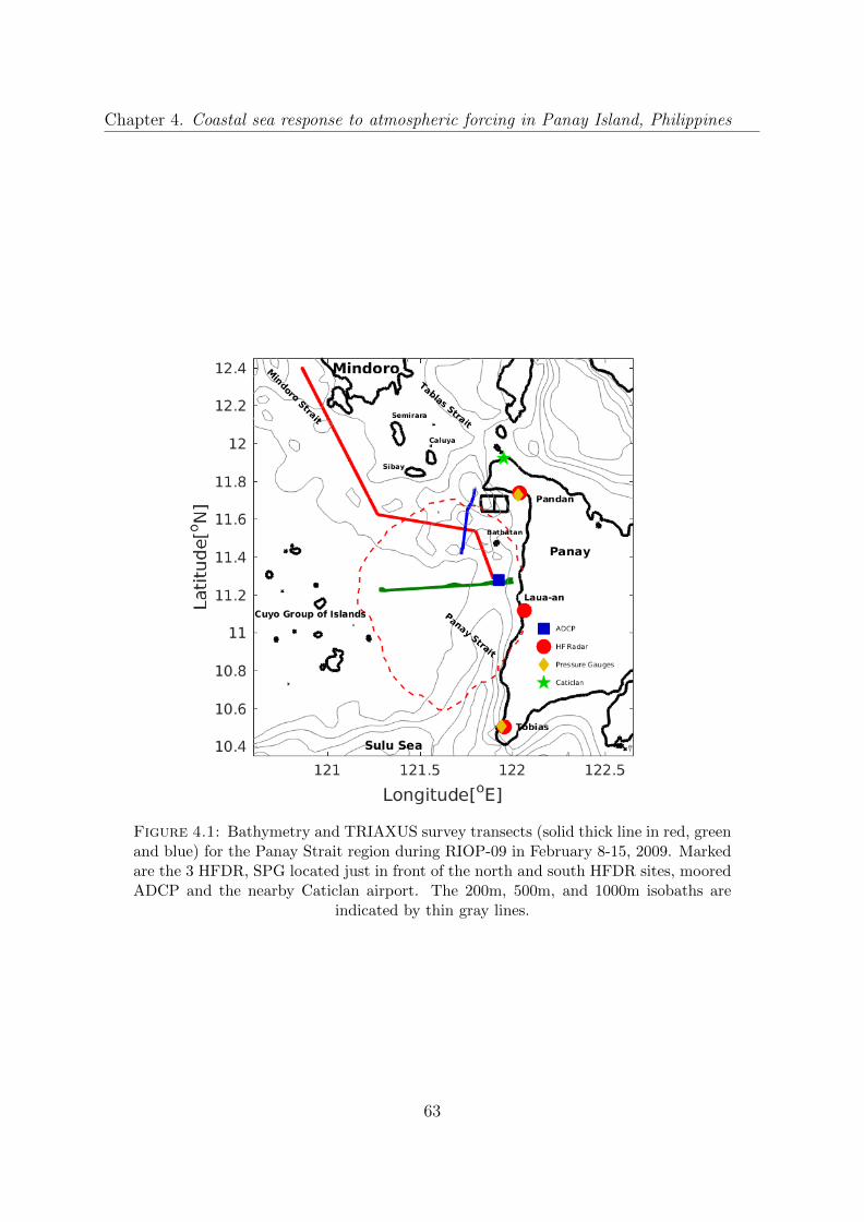
Chapter 4. Coastal sea response to atmospheric forcing in Panay Island, Philippines
Figure 4.1: Bathymetry and TRIAXUS survey transects (solid thick line in red, greenand blue) for the Panay Strait region during RIOP-09 in February 8-15, 2009. Markedare the 3 HFDR, SPG located just in front of the north and south HFDR sites, mooredADCP and the nearby Caticlan airport. The 200m, 500m, and 1000m isobaths are
indicated by thin gray lines.
63
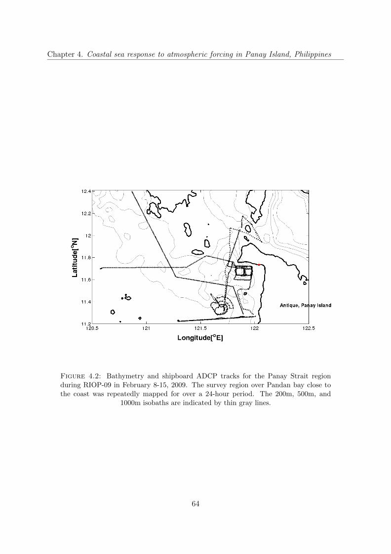
Chapter 4. Coastal sea response to atmospheric forcing in Panay Island, Philippines
Figure 4.2: Bathymetry and shipboard ADCP tracks for the Panay Strait regionduring RIOP-09 in February 8-15, 2009. The survey region over Pandan bay close tothe coast was repeatedly mapped for over a 24-hour period. The 200m, 500m, and
1000m isobaths are indicated by thin gray lines.
64

Chapter 4. Coastal sea response to atmospheric forcing in Panay Island, Philippines
Figure 4.3: (top) Surface current from HFDR and from shipboard ADCP. (bottom)Major surface flows observed are the cyclonic Panay eddy, the northward Panay coastal
jet and the small cyclonic eddy at the tip of Northwest Panay peninsula.
65

Chapter 4. Coastal sea response to atmospheric forcing in Panay Island, Philippines
Figure 4.4: Near-surface current from shipboard ADCP 12 m depth bin and the pre-vailing wind from the Caticlan airport during two successive surveys on (top) February8-10, 2009 and (bottom) February 12-15, 2009. The sampling time from start to end areshown with increasing lighter shadings. The current and wind vectors are color-coded
accordingly.
66
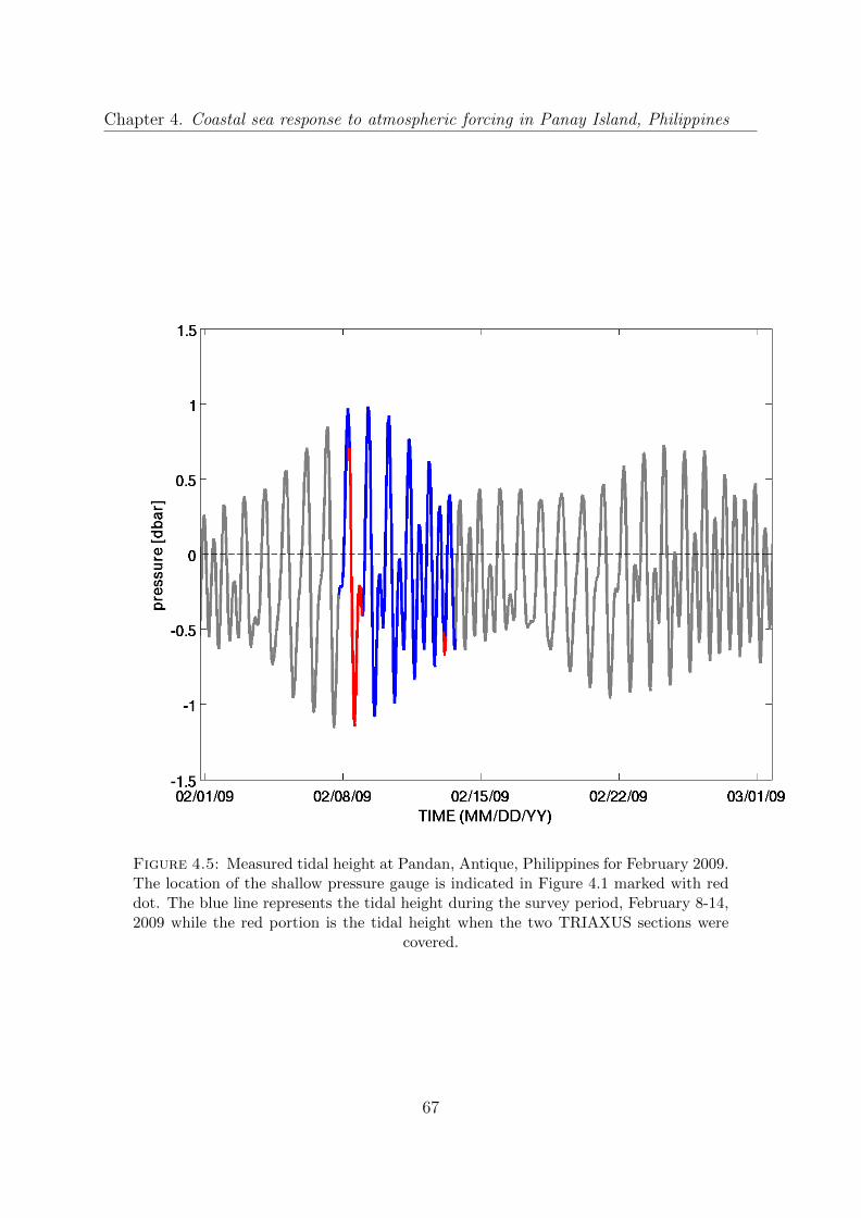
Chapter 4. Coastal sea response to atmospheric forcing in Panay Island, Philippines
Figure 4.5: Measured tidal height at Pandan, Antique, Philippines for February 2009.The location of the shallow pressure gauge is indicated in Figure 4.1 marked with reddot. The blue line represents the tidal height during the survey period, February 8-14,2009 while the red portion is the tidal height when the two TRIAXUS sections were
covered.
67
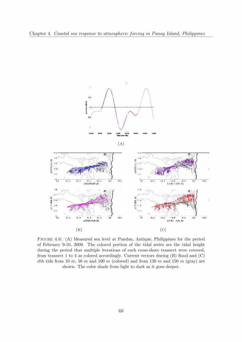
Chapter 4. Coastal sea response to atmospheric forcing in Panay Island, Philippines
(a)
(b) (c)
Figure 4.6: (A) Measured sea level at Pandan, Antique, Philippines for the periodof February 9-10, 2009. The colored portion of the tidal series are the tidal heightduring the period that multiple iterations of each cross-shore transect were covered,from transect 1 to 4 as colored accordingly. Current vectors during (B) flood and (C)ebb tide from 10 m, 50 m and 100 m (colored) and from 130 m and 150 m (gray) are
shown. The color shade from light to dark as it goes deeper.
68
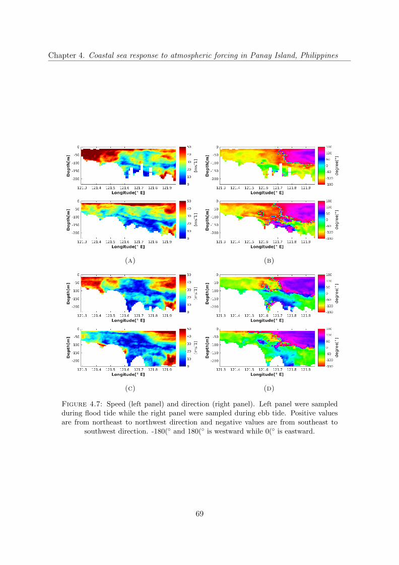
Chapter 4. Coastal sea response to atmospheric forcing in Panay Island, Philippines
(a) (b)
(c) (d)
Figure 4.7: Speed (left panel) and direction (right panel). Left panel were sampledduring flood tide while the right panel were sampled during ebb tide. Positive valuesare from northeast to northwest direction and negative values are from southeast to
southwest direction. -180(◦ and 180(◦ is westward while 0(◦ is eastward.
69

Chapter 4. Coastal sea response to atmospheric forcing in Panay Island, Philippines
(a) (b)
(c)
Figure 4.8: (A) Measured sea level at Pandan, Antique, Philippines for the period ofFebruary 13-14, 2009. The colored portion of the tidal series are the tidal height duringthe period that the (B) tip of Panay and (C) multiple iterations of each survey trackswere performed, as colored accordingly. The near-surface currents from 12 m depth binwere labelled with time in hours, left panel (C) were sampled during ebb tide while theright panel (C) during spring tide. The prevailing mean daily wind during February
13-15, 2009 from the nearby airport is shown (blue to green color).70

Chapter 4. Coastal sea response to atmospheric forcing in Panay Island, Philippines
(a)
(b) (c)
(d) (e)
Figure 4.9: (A) Measured sea level at Pandan, Antique, Philippines for the period ofFebruary 13-14, 2009. The colored portion of the tidal series are the tidal height duringflood (B) and ebb (C) tides TRIAXUS survey. The overlapping tracks were colored ingray during flood tide. The points are labelled with time in hours. (D) Temperature,salinity, (E) density and chlorophyll profiles from survey tracks covered above. Vertical
dotted lines indicate the time on the tracks.71
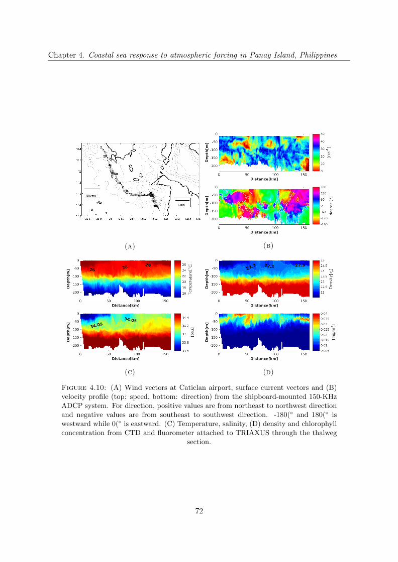
Chapter 4. Coastal sea response to atmospheric forcing in Panay Island, Philippines
(a) (b)
(c) (d)
Figure 4.10: (A) Wind vectors at Caticlan airport, surface current vectors and (B)velocity profile (top: speed, bottom: direction) from the shipboard-mounted 150-KHzADCP system. For direction, positive values are from northeast to northwest directionand negative values are from southeast to southwest direction. -180(◦ and 180(◦ iswestward while 0(◦ is eastward. (C) Temperature, salinity, (D) density and chlorophyllconcentration from CTD and fluorometer attached to TRIAXUS through the thalweg
section.
72
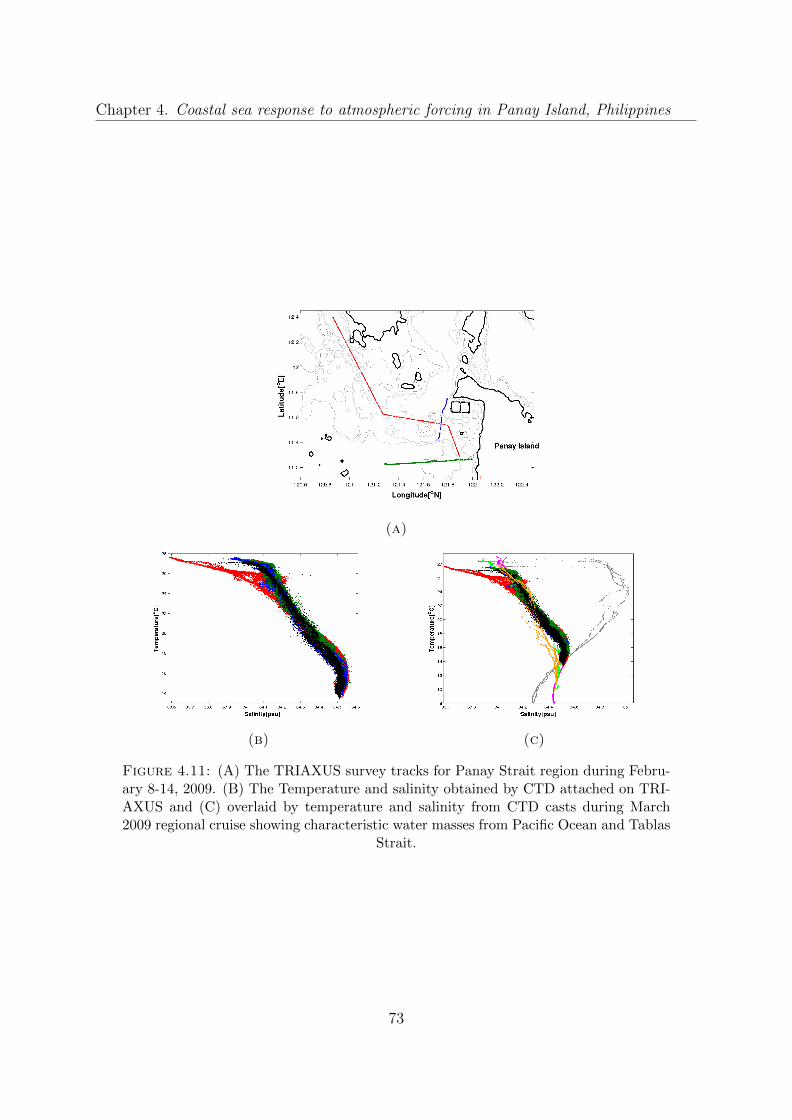
Chapter 4. Coastal sea response to atmospheric forcing in Panay Island, Philippines
(a)
(b) (c)
Figure 4.11: (A) The TRIAXUS survey tracks for Panay Strait region during Febru-ary 8-14, 2009. (B) The Temperature and salinity obtained by CTD attached on TRI-AXUS and (C) overlaid by temperature and salinity from CTD casts during March2009 regional cruise showing characteristic water masses from Pacific Ocean and Tablas
Strait.
73

Chapter 4. Coastal sea response to atmospheric forcing in Panay Island, Philippines
Figure 4.12: (top) 6-day medianed sea level anomalies (cm) and temperature (redline, (◦C/10) ) from Pandan shallow pressure gauge overlaid with wind vectors (ms−1)from the closest QuikSCAT data. Correlations, R between zonal, U and meridional, Vwind component with sea level (left) and temperature (right) are indicated on the top
of the plot. (bottom) The corresponding salinity (psu) anomalies.
74

Chapter 4. Coastal sea response to atmospheric forcing in Panay Island, Philippines
(a)
(b)
Figure 4.13: The 24-hour mean velocity profile from the NW corner of Panay Island.(A) Current vectors from 10m, 75m, and 125m with increasingly lighter shadings. (B)On top is the speed while on the bottom is the direction. Positive values are fromnortheast to northwest direction (white to red contour) and negative values are fromsoutheast to southwest direction (white to blue contour). The y-axis is the distance
marked in Figure 4.23 A.
75

Chapter 4. Coastal sea response to atmospheric forcing in Panay Island, Philippines
Figure 4.14: Sea surface Temperature (SST) for the Philippine Archipelago. Theimage is a 1 km composite of MODIS Aqua sensor image for the period February 7 to13, 2009 (top) and the 6 km daily Group for High Resolution Sea Surface Temperature(GHRSST) Level 4 SST data (daily mean values provided by Physical Oceanogra-phy DAAC (http://podaac.jpl.nasa.gov/dataset/UKMO-L4HRfnd-GLOB-OSTIA) av-
eraged over the same time period (bottom).
76

Chapter 4. Coastal sea response to atmospheric forcing in Panay Island, Philippines
Figure 4.15: Mean profile of temperature, salinity and chlorophyll concentrationacross the PL eddy during the hydrographic survey (February 8-9, 2009).
77
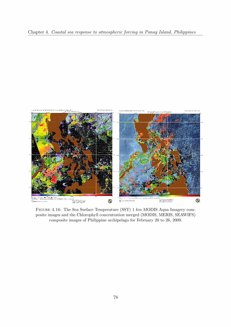
Chapter 4. Coastal sea response to atmospheric forcing in Panay Island, Philippines
Figure 4.16: The Sea Surface Temperature (SST) 1 km MODIS Aqua Imagery com-posite images and the Chlorophyll concentration merged (MODIS, MERIS, SEAWIFS)
composite images of Philippine archipelago for February 20 to 26, 2009.
78

Chapter 5
Barotropic and baroclinic tides in
Panay Strait, Philippines
5.1 Abstract
The Panay Strait constitutes a topographically complex system with intense tidal cur-
rents. The four major tidal constituents in the total energy spectra inferred from sea level
and current profiles are K1, O1, M2, and S2. Spatially, O1 and M2 dominate over K1 and
S2, respectively. The diurnal tide accounts for highest amplitude variability over the shal-
low shelf while semi-diurnal tides over the deeper channel of the strait. Rotary spectra of
surface currents shows inertial frequency peaks and exhibit an unusually broad peak in
both the clockwise (CW) and counterclockwise (CCW) rotating components, indicating
frequency shift by the vorticity of sub-inertial currents prevalent in the region. Vertically,
variance of the horizontal velocity explained by the major tidal constituents peaks in two
distinct depth bands; the upper layer centered at 110 m (11% variance) dominated by
semi-diurnal tide (M2) and the lower layer at 470 m (26% variance) dominated by diurnal
tides (O1). Semi-diurnal tidal current ellipses (M2 and S2) exhibit a dominance of CW
motions at near-surface depth (110m), indicative of downward energy propagation and
implying a surface energy source. These features from Acoustic Doppler Current Profiler
(ADCP) deployed close to the sill is consistent with the dominant semi-diurnal tide (M2)
over the channel of the strait from the High Frequency Doppler Radar (HFDR). Com-
parison of incoherent to coherent tidal energy shows K1 dominated the incoherent tidal
79

Chapter 5. Barotropic and baroclinic tides in Panay Strait, Philippines
band. Spatially, incoherent energy is dominant over the channel particularly near the sill
and the constricted part of the strait. The incoherent portion of the tide is presumably
attributable to the surface expression of the internal tide which seems to be generated
near the sill and then topographically steered west over the edge of the shallow shelf
where incoherent energy is dominant.
5.2 Introduction
Tidal currents constitute the most ubiquitous signal in the coastal ocean. They can
be difficult to interpret as they vary at multiple topographic scales. The Philippine
archipelago bounded by the Pacific Ocean on the east and South China Sea (SCS) on
the west, consists of a complex array of islands, embayments and seas connected by
multitude of straits and sills. The barotropic (depth-independent) tidal components are
significant in the region with strikingly different geographical structures, dominated by
semi-diurnal tides in the Pacific and diurnal tides in the SCS. Within the Philippines,
strong barotropic tidal flows through many of the passages reflect the substantial tidal
surface height differences between the Pacific and SCS, as well as acceleration through
topographic constrictions.
Tidal currents flowing over topography in a stratified ocean give rise to baroclinic internal
tides. In the interior Philippine seas, the largest known internal tide sources are in the
Sibutu Passage, south of Sulu Sea (SS)[Zhang et al., 2010]. A strong surface signature
was illustrated by the Moderate Resolution Imaging Spectroradiometer (MODIS) true
color sunglint image of the western SS [Hurlburt et al., 2011] and simulations of tides in
the Philippine archipelago clearly represent this surface signal and further indicates that
internal tides are pervasive within the Philippine seas. Jackson et al. [2011] found internal
waves observed by satellite imagery and Girton et al. [2011] from in situ data in several
areas within the Philippine archipelago. Likewise, Apel et al. [1985] found internal tidal
beams generated in Sibutu Passage that propagate across the SS.
Aside from the well-known solitary wave occurrences in the SS [Apel et al., 1985; Hurl-
burt et al., 2011; Tessler et al., 2010] and the Sulu Archipelago [Jackson et al., 2011],
concentrations of nonlinear internal wave activity on the shelf region (Cuyo Shelf) at
80
Chapter 5. Barotropic and baroclinic tides in Panay Strait, Philippines
the northern end of the SS between Palawan and Panay islands was observed in syn-
thetic aperture radar (SAR) and optical sunglint satellite imagery ([Jackson et al., 2011].
These waves dissipate over the shallower shelf region after 2.5days of traveling from sev-
eral locations in the Sulu Archipelago [Jackson et al., 2011]. Simulations of tides in
the Philippine seas by 1/12◦ Hybrid Coordinate Ocean Model (HYCOM) also note the
strong sea surface height signature of internal tides in Mindoro strait [Hurlburt et al.,
2011]. Internal wave measurements from two McLane Labs moored profilers (MMP) at
either end of Mindoro-Panay Straits illustrate some similarities and dramatic contrasts
over fairly short distances within archipelagic topography. There are more energies to
both the diurnal and semidiurnal frequency band in Mindoro Strait to the SCS while
at lower (sub-inertial) frequencies with larger isopycnal displacement at depth, south of
Panay Strait entering into the SS [Chinn et al., 2012].
The Panay Strait serves as the major path way of water from the SCS via the Mindoro
Strait to SS (Figure 5.1). A small basin ( 1300m deep) known as the Semirara Sea
separates the Panay Strait from the Mindoro Strait on the northwest and Tablas Strait
on the northeast. A sill of 578 m depth forms the shallowest point within the strait.
Defining the 100m isobath as the outer edge of the shelf, Panay Strait is bordered by
the wider Cuyo shelf on the west and the very narrow Panay shelf on the east. On the
shelf lies the low lying Cuyo Group of Islands and extensive reefs. The Panay Strait
thus constitutes a topographically complex system of small low-lying islands, seamounts,
shelves, sills, and a deep basin that may be a locale of intense tidal currents.
This study is primarily directed towards determining the structure of the barotropic
and baroclinic tide in Panay Strait. Knowledge of oceanic processes, specifically tides is
important to understand their specific impact on the currents, stratification, and nutrient
distributions in the region.
5.3 Methods
For the description of tidal sea level and current oscillations, data from HFDR measure-
ments, one moored ADCP and two shallow pressure gauges (SPG) were used. Their
record lengths vary from 368 to 646 days (Figure 5.2) with about 142 days of overlap.
81

Chapter 5. Barotropic and baroclinic tides in Panay Strait, Philippines
Failures in HFDR occurred at sites due to electrical power loss primarily because of burned
power cables and generator failures during black-outs. In times when data are lost from
one site, two sites were used to calculate vector currents. During the deployment period,
the largest data loss was during the bistatic calibration performed from December 22,
2008 to January 9, 2009. Moored instruments were deployed and retrieved at different
times, and overlaps of uninterrupted coverage were selected for analysis.
The HFDR current vectors underwent minor quality control prior to the analysis. Missing
data segments were subject to temporal interpolation [Chavanne et al., 2007] in which a
constant linear trend and sinusoids at M2, K1 and inertial frequencies were least squares
fitted to the observations available in a 3-day window centered on each missing data
segment shorter than 36 hours. The fit was performed only if more than 36 observations
were available. This interpolation was carried out on hourly vector currents.
In conjunction with the HFDR, an ADCP mooring was deployed as part of the Ex-
ploratory Cruise on the R/V Melville in June 2007 to provide aspects of the full three-
dimensional circulation in Panay Strait. An upward-looking RDI Teledyne Long Ranger
75-kHz, bottom mounted ADCP (11.2790 ◦N , 121.9244 ◦E) was located inside the re-
gion covered by HFDR, 2.5 km downstream from the narrowest constriction at Panay
Sill of 578 m water depth. The passage width is 36 km determined between the 100
m isobaths on either side of the mooring as surveyed by multibeam echosounder. The
ADCP included pressure and temperature sensors. Sampling rates were set to resolve the
tides, and were 30 minutes for the ADCP and 15 minutes for the temperature sensors.
The mooring was recovered in March 2009.
The ADCP returned 100 % of the velocity time series. However, due to surface reflec-
tion contamination, the bottom-mounted ADCP was unable to resolve the near surface
velocity (upper 50 m). Pressure time series were used to correct for mooring blowover.
The velocity data were then linearly interpolated onto a 10 m depth grid and a common
time base of 1 hour.
As part of the PhilEx program, an array of shallow pressure gauges was deployed at
approximately 5 - 10 m depth along Panay Strait (Pandan and Tobias Fornier, Antique).
The location, deployment period and length of observation of the pressure gauges are
provided in Figure 5.1 and (Figure 5.2). Absolute pressure is measured every ten seconds
by a Paroscientific quartz pressure sensor with an accuracy of 0.3 mb (-1 % of the signal).
82

Chapter 5. Barotropic and baroclinic tides in Panay Strait, Philippines
The data were averaged into hourly bins and were used to examine possible influences of
sea level to the tidal variations in Panay Strait.
Spectral analysis is useful to partition the variance of a time series as a function of
frequency [Emery and Thomson, 2004]. The present study utilizes power spectrum of sea
level and rotary spectral analysis [Gonella, 1972] to the HFDR-derived surface current and
current profile from the moored ADCP. These provide estimates of power (energy density)
distributed over a range of given frequency bins [Press et al., 1996]. Spectral estimates
were spatially-averaged for surface currents and vertically-averaged for the ADCP current
profile. The sea level spectra were further assessed to extract the tidally-driven current
from the time-series data.
HFDR and ADCP current components (zonal and meridional) and sea level, were har-
monically analyzed using the T-Tide Matlab package [Pawlowicz et al., 2002] over the
deployment period of each instrument. Four significant tidal constituents (K1, O1, M2,
S2) inferred from sea level were least square fitted to the hourly observations, along with a
constant and a linear trend. The 95 % confidence intervals were computed by a bootstrap
method. Maps of tidal current ellipses, major axis amplitudes and phases will be use to
characterize the surface tidal currents.
5.4 Results and Discussions
5.4.1 Tidal components inferred from sea level
Phase-locked tidal sea level explains 95.1 % and 96.9 % of the total sea level variance over
a year (425 days) from hourly records from Pandan and Tobias Fornier, respectively. The
frequency spectra of sea level variations shows energy peaks at four major constituents
(K1, O1, M2, and S2) (Figure 5.3).
The contribution of major constituents to the total energy spectra of sea level is shown
in Figure 5.4. An increase in the variance is largely attributed to K1, O1, M2, and S2,
respectively. These four major constituents will therefore be use to extract tides for
analysis.
83
Chapter 5. Barotropic and baroclinic tides in Panay Strait, Philippines
5.4.2 Horizontal structure of the tidal components inferred from
HFDR
The most energetic surface current variations for periods shorter than 5days are inertial
and tidal currents. The spectral properties of surface currents within the radar domain
shows diurnal peaks centered on K1 and O1, semi-diurnal on M2 and S2, and inertial
frequency on fi with period of 62 hours ( 2.59 days) at 11.1◦N (Figure 5.5). The O1, K1,
M2 and a much weaker S2 are the most significant with minor contributions from other
constituents. Higher harmonics of diurnal and semi-diurnal constituents also display
significant peaks.
The rotary spectra decomposes a vector time series into CW and CCW rotating com-
ponents by frequency. At near-inertial periods, the CW predominates in the Northern
Hemisphere due to the action of the Coriolis force to the right of the velocity vector.
This is evident in the spectrum where inertial frequencies have more energy in the CW
rotating band as expected and are unusually broad (maximum 1.46 m2s−2.cph−1), pos-
sibly frequency-shifted due to vorticity of sub-inertial currents (see Chapter 3) and the
forcing by wind, both prevalent during NE monsoon [Pullen et al., 2008]. For diurnal
and semi-diurnal frequency bands, CW motions are also more energetic than the CCW
components by 1.47 m2s−2.cph−1 and 1.18 m2s−2.cph−1, respectively.
Variance explained by the four major tidal constituents constitute 5.7 % and 9.4 % of
the total variance of zonal and meridional current components over the 1-year record,
respectively (Figure 5.6). The highest variance for the zonal current component is over
the deep channel further south of the sill and for the meridional component north of
the sill near a sharp bend in bathymetry where the Island of Batbatan is located. The
semidiurnal tide contributed much to the highest variance over the deep channel while
the diurnal tide over the shallow shelf (Figure 5.7).
To determine the relative contribution of the tidal currents to the mean kinetic and
mean eddy kinetic energies (EKE), those parameters were calculated and are shown in
Figure 5.8. The tidal currents, up and vp were formed from the four major tidal current
constituents analysed. EKE tends to be greatest where the mean circulation is strongest
west of the radar domain, over the shelf but low on the east along the coast. This implies
that the seasonal PL eddy derived more of its energy from the seasonal return flow as
84

Chapter 5. Barotropic and baroclinic tides in Panay Strait, Philippines
a consequence to the positive Ekman pumping generated over this region during NEM
regime and less energy from the persistent Panay coastal (PC) jet as the eastern limb
of the PL eddy. In comparison, the mean tidal current kinetic energy is an order of
magnitude less than both the mean current and mean EKE.
The relative contribution of the tidal currents to the mean kinetic energy was estimated
by the ratio:
Rtmke =u2p(x, y) + v2p(x, y)
u2(x, y) + v2(x, y)(5.1)
where u and v are observed current velocities and the overbar denotes a time mean of
over a year record and, x and y denotes the conventional Cartesian coordinates.
Similarly, the contribution of the tidal currents to the mean eddy kinetic energy was
estimated by
Rteke =u2p(x, y) + v2p(x, y)
u′2(x, y) + v′2(x, y)(5.2)
where the primed quantities denote deviations from the time mean over a year.
The distributions of Rtmke and Rteke are shown in Figure 5.9, while the distributions of
O1 and M2 constituents, which contribute much to the tidal kinetic energy, are shown in
Figure 5.10.
The contributions of the tidal currents to both the mean current and the mean EKE show
similar patterns though their contribution to the mean eddy kinetic energy is relatively
large (Rtmke = 0.043 and Rteke = 0.0510). The regions with highest contributions are
on the shallow areas of the Cuyo shelf where there are sharp bends in the 100 m isobath
and over which the persistent northward PC jet exists. This suggests the influence of
tidal currents on the PC jet, as it accelerates over the shallow part of the shelf. Another
high contribution is on the west end of the radar domain, where a strong return flow
indicating the PL eddy approaches the 100 m isobath of the shallow Cuyo shelf.
From the 4 major constituents, O1 and M2 contribute the highest to the mean tidal
kinetic energy where O1 dominates over the shallow shelf while M2 over the deep channel
85

Chapter 5. Barotropic and baroclinic tides in Panay Strait, Philippines
with sharp bends observed in the 100 m isobath and over which PC jet intensifies as it
approach the narrowest constriction of the strait.
5.4.3 Vertical structure of the tidal component inferred from
ADCP
For the mooring located near the relatively narrow part of Panay Strait, tidal variability
makes up a large part of the velocity signal. The vertically-averaged frequency spectrum
from the ADCP is very similar to the spectrum from HFDR for periods shorter than 5
days showing strong peaks at K1, O1, M2, and S2 tidal components (Figure 5.11). The O1
and M2 constituents dominate the diurnal and semi-diurnal bands, respectively. Strong
energy in the inertial band is absent in the spectrum, presumably because the data in
the upper profile (top 50 m) are missing. This suggests the importance of the local wind
in generating the peaks in the near-inertial motions from HFDR-derived surface current
spectrum.
The large percentage of variance explained by the 4 major tidal constituents (K1, O1, M2,
and S2) are in two distinct layers, centered at 110 m and 470 m for both across and along-
channel tidal current components (Figure 5.12). The highest variance at 110 m (11.32 %)
accounts for the along-channel tidal currents which corresponds to the strong shear where
upper layer flows northward into the SCS while strong southward flow below into the Sulu
Sea during the NEM regime. The M2 constituents mainly contribute to the variance. At
470 m, across-channel tidal currents account for the highest variance (26.33%) which
corresponds with the intense thermocline near-inertial motions suggested to be due to
Parametric Subharmonic Instability (PSI) of the diurnal internal tide found near 400 m
at northern Mindoro Strait in the SCS, which undergoes similar or higher levels of near-
bottom mixing than the Panay sill [Chinn et al., 2012]. Chinn et al. [2012] note that
PSI of the internal tide can only occur equatorward of the critical latitude where half
the tidal frequency is greater than the local inertial frequency (e.g., 14.52 ◦ N for K1 and
13.44 ◦ N for O1 ). Recent observational work under PhilEx program however, has shown
convincing evidence that near the critical latitudes the rates of PSI are vastly enhanced
and may be a dominant part of the redistribution of energy throughout the internal wave
spectrum [Chinn et al., 2012]. The main evidence for PSI was the fortnightly modulation
of the near-inertial band, indicating a signal that is often comprised of both upward and
86
Chapter 5. Barotropic and baroclinic tides in Panay Strait, Philippines
downward propagating waves seen near 400 m [Chinn et al., 2012]. The specifics of the
physical forcing that allow it to occur at this particular depth however, are uncertain
and more work is needed to fully understand the dynamics at work in Mindoro-Panay
Strait. The variance explained by mean tidal across-channel currents is attributed mostly
to diurnal tide (O1) over the Cuyo shelf to the west.
The vertical mean kinetic energy, eddy kinetic energy and tidal kinetic energy are shown
in Figure 5.13. In contrast to the kinetic energies from the surface current, the mean eddy
and the mean tidal current kinetic energies are relatively small, an order of magnitude
less and two orders of magnitude less, respectively than the mean current kinetic energy.
The mean current kinetic energy is highest at 520-m depth which corresponds with the
hydraulically controlled benthic overflow derived from approximately 400 m deep in the
SCS that acts to ventilate the Sulu Sea with little seasonal variance [Tessler et al., 2010].
Both the highest mean eddy and tidal current kinetic energies are at 470 m depth where
a PSI-generated near-inertial wave signal was found by Chinn et al. [2012].
The vertical distributions of Rtmke and Rteke are shown in Figure 5.14 with a peak at
110 m and two distinct peaks at 110 m and 470 m, respectively, indicating the dominant
tidal activities at shear depth ( 110 m) during NEM and confirming the PSI-generated
thermocline near-inertial motions at 470 m depth discussed above.
5.4.4 Coherent tides
Harmonic analyses of surface and sub-surface current components (zonal and meridional)
were performed using T-tide Matlab package [Pawlowicz et al., 2002]. Only the 4 major
(K1, O1, M2, and S2) tidal constituents inferred from sea level were least-square fitted to
the observations, along with a constant and a linear trend.
Maps of the observed tidal current ellipses, major axis amplitudes and phases of the
four major constituents (K1, O1, M2, and S2) are shown in Figure 5.15. Tidal ellipses
are a compact method used to describe tidal current variance using major and minor
axes (Amaj and Amin), inclination and phase. The axes describe the magnitude of the
current in 2 orthogonal directions, inclination provides orientation for the axes and phase
indicates time lag from Greenwich when the time vector passes the northern semi-major
axis. Diurnal peaks are more pronounced over the shelf with amplitudes increasing to the
87

Chapter 5. Barotropic and baroclinic tides in Panay Strait, Philippines
shallow area. O1 tidal ellipses are elliptical over the shelf, relatively narrow, and aligned
along the channel axes. M2 has broader and more circular tidal ellipses north of the
strait, indicating that rotation is relatively important and/or due to transverse reflection
effects. The M2 major axis amplitudes increase towards the narrow constricted part of
the strait. S2 has similar patterns to M2 though substantially weaker. The large phase
gradients across the HFDR coverage indicate strong reversing tidal pressure gradients
and likely locations of accelerated currents and internal tide generation. This is most
obvious at the deep channel near the sill and at the edge of the shallow shelf with shoals
and promontories.
The vertical structure of the tidal ellipses of 4 major tidal constituents (O1,K1, M2 and
S2) remarkably exhibit two sharp peaks consistent with the location of highest variance
explained by the tides at 110 m and 470 m, suggesting contributions from baroclinic tidal
current. The coherent portion of the semi-diurnal tide (M2) dominates at 110 m while
the coherent diurnal tide (O1) dominates at 470 m, consistent with the PSI of the diurnal
internal tide found at this depth by Chinn et al. [2012].
5.4.5 Ratio of Incoherent to Coherent Energy
Observed ratios of the averaged diurnal and semi-diurnal power spectra for residual cur-
rents and tidal currents are shown in Figure 5.17).
The diurnal frequency band was defined as:
[O1 + 1/T >diurnal >K1 – 1/T]
and the semi-diurnal frequency band as:
[M2 + 1/T >semi-diurnal >S2 – 1/T]
where T is the record length.
The K1 constituent dominated the incoherent tidal band, (note the difference in scale,
Figure 5.17). Incoherent diurnal energy is strong over the northern region of the channel
in between the shoals, slightly further down south towards the sill and again increased
into the Sulu Sea (Figure 5.17A). The incoherent semi-diurnal energy is most significant
in the more confined regions than the diurnal, between the shoals north of the channel
88
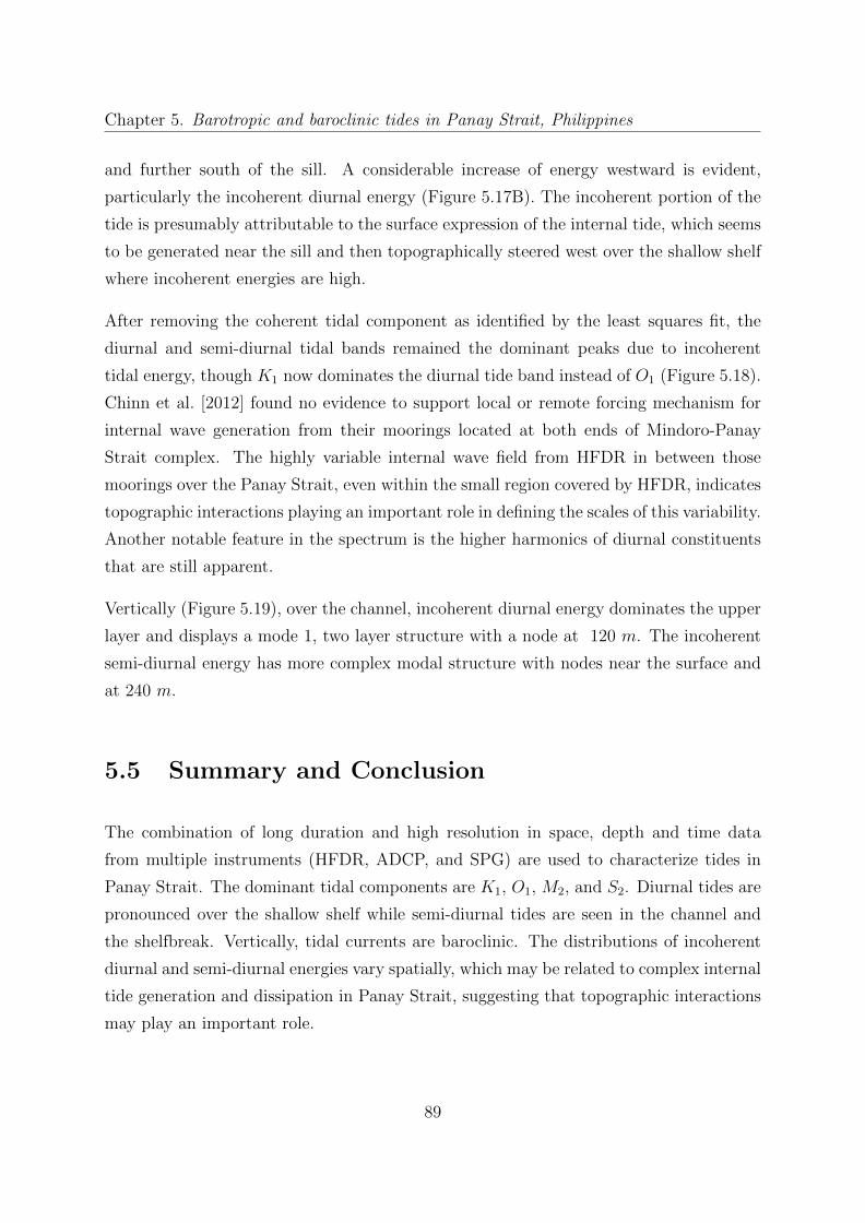
Chapter 5. Barotropic and baroclinic tides in Panay Strait, Philippines
and further south of the sill. A considerable increase of energy westward is evident,
particularly the incoherent diurnal energy (Figure 5.17B). The incoherent portion of the
tide is presumably attributable to the surface expression of the internal tide, which seems
to be generated near the sill and then topographically steered west over the shallow shelf
where incoherent energies are high.
After removing the coherent tidal component as identified by the least squares fit, the
diurnal and semi-diurnal tidal bands remained the dominant peaks due to incoherent
tidal energy, though K1 now dominates the diurnal tide band instead of O1 (Figure 5.18).
Chinn et al. [2012] found no evidence to support local or remote forcing mechanism for
internal wave generation from their moorings located at both ends of Mindoro-Panay
Strait complex. The highly variable internal wave field from HFDR in between those
moorings over the Panay Strait, even within the small region covered by HFDR, indicates
topographic interactions playing an important role in defining the scales of this variability.
Another notable feature in the spectrum is the higher harmonics of diurnal constituents
that are still apparent.
Vertically (Figure 5.19), over the channel, incoherent diurnal energy dominates the upper
layer and displays a mode 1, two layer structure with a node at 120 m. The incoherent
semi-diurnal energy has more complex modal structure with nodes near the surface and
at 240 m.
5.5 Summary and Conclusion
The combination of long duration and high resolution in space, depth and time data
from multiple instruments (HFDR, ADCP, and SPG) are used to characterize tides in
Panay Strait. The dominant tidal components are K1, O1, M2, and S2. Diurnal tides are
pronounced over the shallow shelf while semi-diurnal tides are seen in the channel and
the shelfbreak. Vertically, tidal currents are baroclinic. The distributions of incoherent
diurnal and semi-diurnal energies vary spatially, which may be related to complex internal
tide generation and dissipation in Panay Strait, suggesting that topographic interactions
may play an important role.
89

Chapter 5. Barotropic and baroclinic tides in Panay Strait, Philippines
Figure 5.1: Map of study area. Bathymetry contours are in meters. The color barrepresents color depth in meters. Instrument locations are indicated as follows: HFDR(red circle), moored ADCP (magenta square), and SPG (yellow diamond). The magenta
dashed lines indicates 75 % coverage of the HFDR.
90

Chapter 5. Barotropic and baroclinic tides in Panay Strait, Philippines
Figure 5.2: Temporal coverage of the instruments. The thickness corresponds to thepercentage of grid points with data.
91
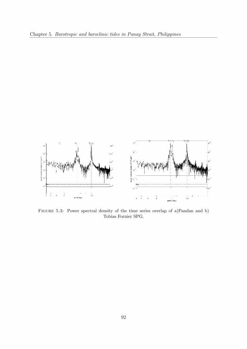
Chapter 5. Barotropic and baroclinic tides in Panay Strait, Philippines
Figure 5.3: Power spectral density of the time series overlap of a)Pandan and b)Tobias Fornier SPG.
92
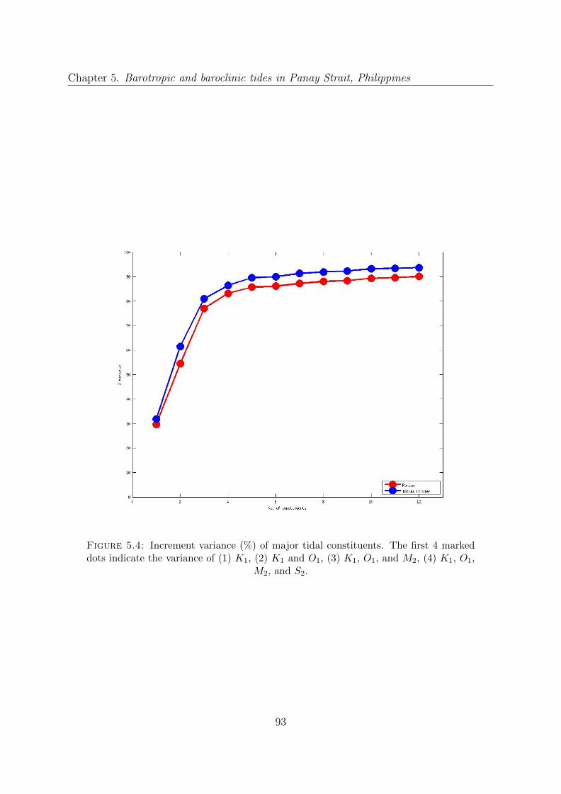
Chapter 5. Barotropic and baroclinic tides in Panay Strait, Philippines
Figure 5.4: Increment variance (%) of major tidal constituents. The first 4 markeddots indicate the variance of (1) K1, (2) K1 and O1, (3) K1, O1, and M2, (4) K1, O1,
M2, and S2.
93

Chapter 5. Barotropic and baroclinic tides in Panay Strait, Philippines
Figure 5.5: Rotary power spectra for one year of HFDR data over 212 grid points withmore than 75% temporal coverage. Major tidal constituents and inertial frequency, fi
are indicated on the top x-axis, indicated by vertical dotted lines.
94

Chapter 5. Barotropic and baroclinic tides in Panay Strait, Philippines
Figure 5.6: Variance explained by 4 major tidal constituents (K1, O1, M2, and S2).
95
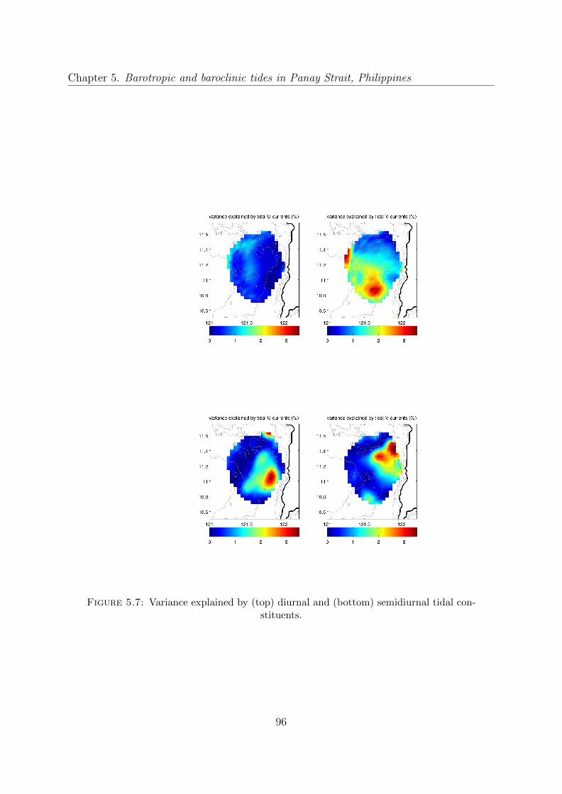
Chapter 5. Barotropic and baroclinic tides in Panay Strait, Philippines
Figure 5.7: Variance explained by (top) diurnal and (bottom) semidiurnal tidal con-stituents.
96
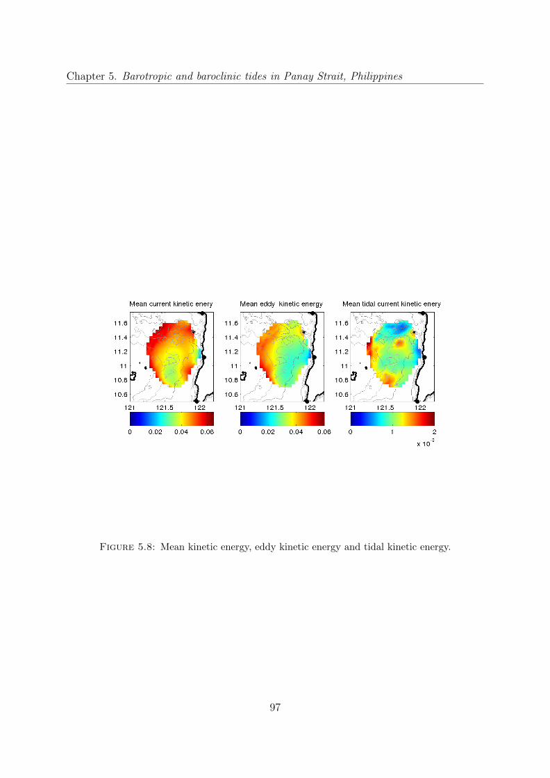
Chapter 5. Barotropic and baroclinic tides in Panay Strait, Philippines
Figure 5.8: Mean kinetic energy, eddy kinetic energy and tidal kinetic energy.
97

Chapter 5. Barotropic and baroclinic tides in Panay Strait, Philippines
Figure 5.9: Contribution of tidal currents to the (A) mean kinetic energy, Rtmke andthe (B) eddy kinetic energy, Rteke.
98
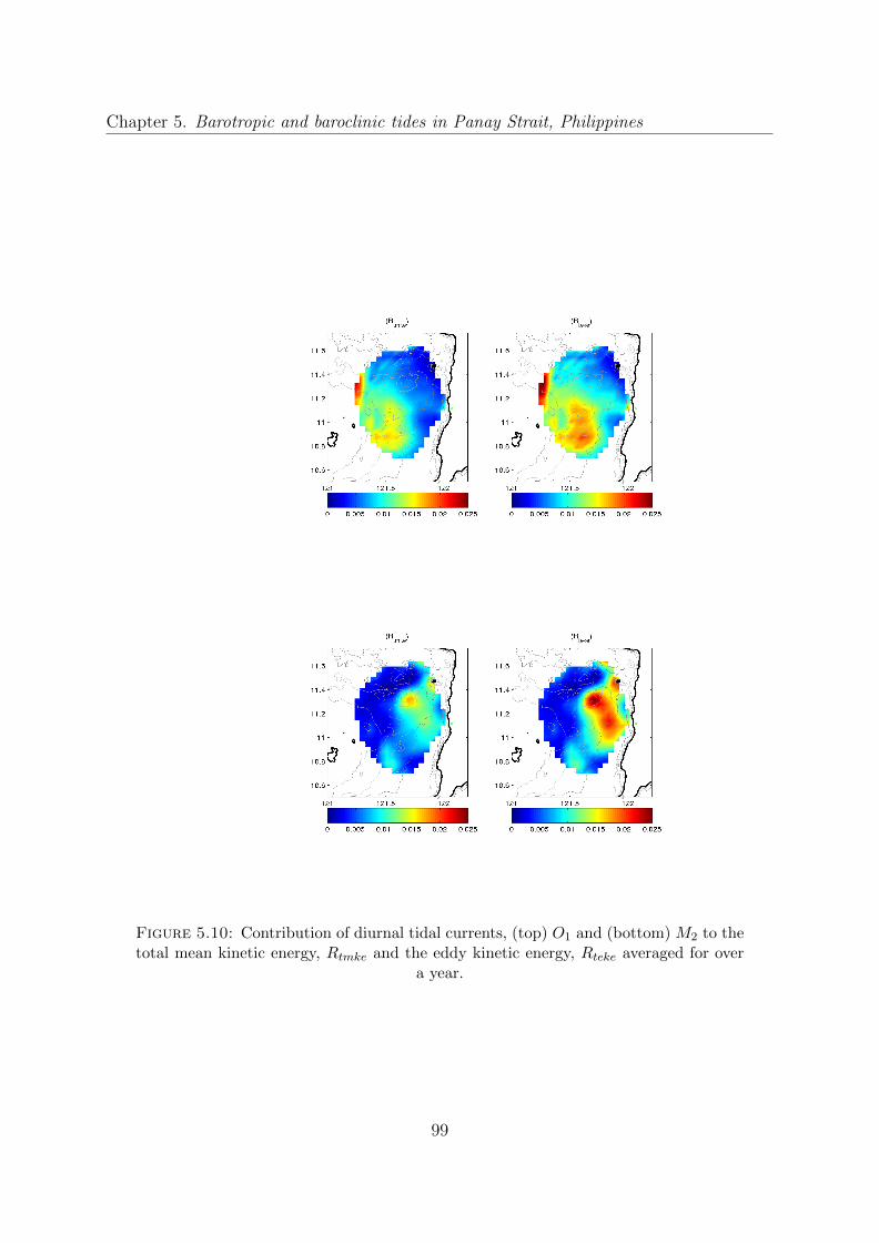
Chapter 5. Barotropic and baroclinic tides in Panay Strait, Philippines
Figure 5.10: Contribution of diurnal tidal currents, (top) O1 and (bottom) M2 to thetotal mean kinetic energy, Rtmke and the eddy kinetic energy, Rteke averaged for over
a year.
99

Chapter 5. Barotropic and baroclinic tides in Panay Strait, Philippines
Figure 5.11: Rotary power spectra from vertically averaged frequency spectra fromADCP. Major tidal constituents and inertial frequency, fi are indicated on the top
x-axis, indicated by vertical dotted lines.
100
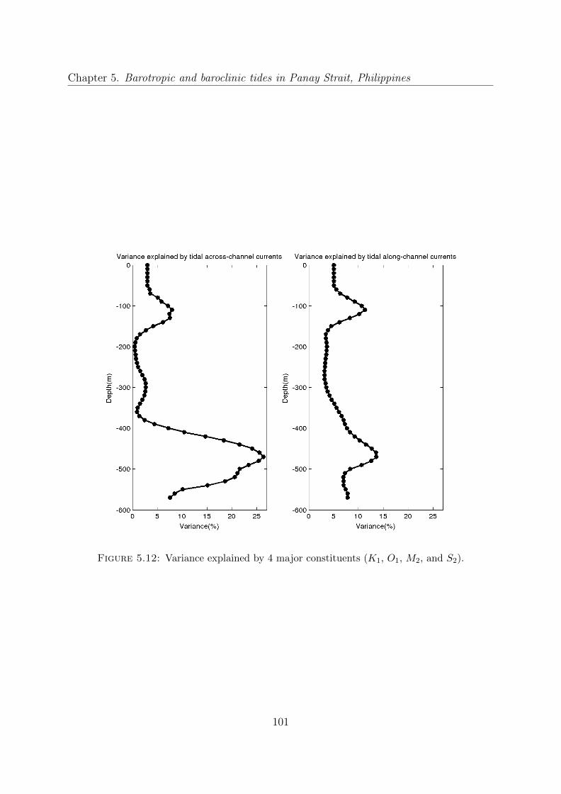
Chapter 5. Barotropic and baroclinic tides in Panay Strait, Philippines
Figure 5.12: Variance explained by 4 major constituents (K1, O1, M2, and S2).
101
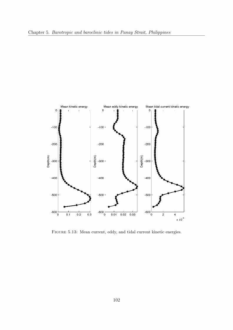
Chapter 5. Barotropic and baroclinic tides in Panay Strait, Philippines
Figure 5.13: Mean current, eddy, and tidal current kinetic energies.
102
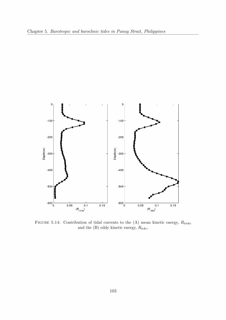
Chapter 5. Barotropic and baroclinic tides in Panay Strait, Philippines
Figure 5.14: Contribution of tidal currents to the (A) mean kinetic energy, Rtmkeand the (B) eddy kinetic energy, Rteke.
103
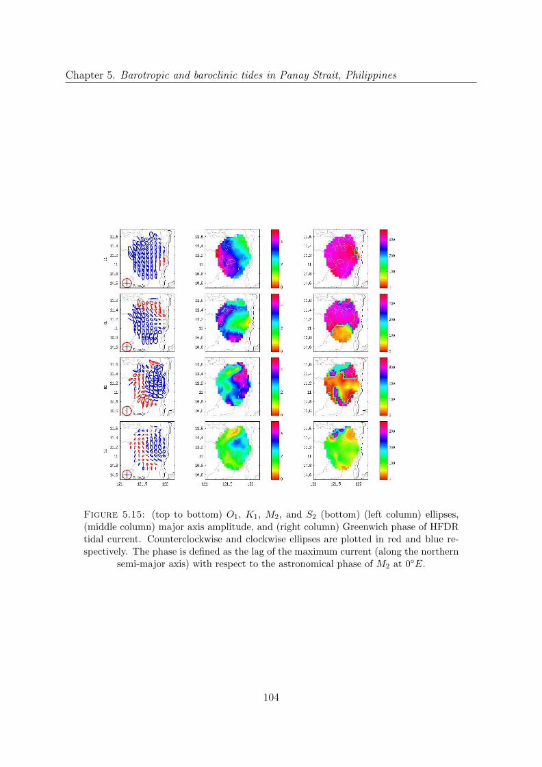
Chapter 5. Barotropic and baroclinic tides in Panay Strait, Philippines
Figure 5.15: (top to bottom) O1, K1, M2, and S2 (bottom) (left column) ellipses,(middle column) major axis amplitude, and (right column) Greenwich phase of HFDRtidal current. Counterclockwise and clockwise ellipses are plotted in red and blue re-spectively. The phase is defined as the lag of the maximum current (along the northern
semi-major axis) with respect to the astronomical phase of M2 at 0◦E.
104

Chapter 5. Barotropic and baroclinic tides in Panay Strait, Philippines
(a) (b)
(c) (d)
Figure 5.16: O1, K1, (top) M2, and S2 (bottom), averaged ellipses with depth Coun-terclockwise and clockwise ellipses are plotted in red and blue respectively.
105

Chapter 5. Barotropic and baroclinic tides in Panay Strait, Philippines
(a)(b)
Figure 5.17: Ratio of incoherent to coherent diurnal and semidiurnal tides as observedin surface current record.
106

Chapter 5. Barotropic and baroclinic tides in Panay Strait, Philippines
Figure 5.18: Rotary power spectra for one year of residual HFDR data over 212 gridpoints with more than 75 % temporal coverage. Major tidal constituents and inertial
frequency, fi are indicated on the top x-axis, indicated by vertical dotted lines.
107
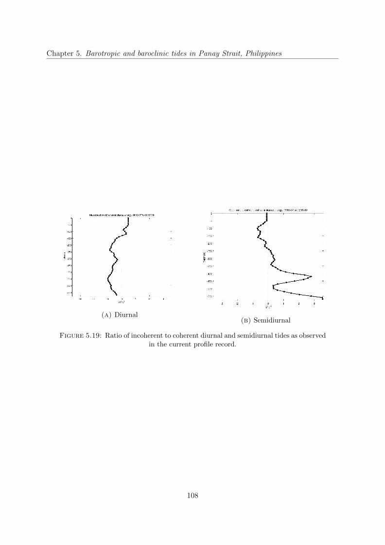
Chapter 5. Barotropic and baroclinic tides in Panay Strait, Philippines
(a) Diurnal(b) Semidiurnal
Figure 5.19: Ratio of incoherent to coherent diurnal and semidiurnal tides as observedin the current profile record.
108

Chapter 6
Summary and Conclusion
The internal Philippine seas have a unique oceanographic environment, with complex
bathymetry confined within the intricate configuration of the Philippine Archipelago con-
nected by multiple array of narrow straits. Strong archipelago throughflow interacts with
abrupt changes in bathymetry within and between the basins, swift tidal currents are
present, while the island orographic effects on the monsoonal reversing winds generate an
energetic wake of eddies through Ekman pumping.
The locally generated mesoscale eddies in the lee of major islands occur west of the
Philippines during the stronger and more stable NE monsoon. In the lee of Mindoro
and Luzon Islands, steady monsoon winds form stationary lee eddies while episodically
strengthened wind jets lead to simultaneous detachment of counter-rotating eddies in
the model, with propagation directions dependent on the orientation of the winds during
monsoon surges [Pullen et al., 2008].
The installed HFDR array in Panay Island, south of Mindoro, produces time series of
2-D maps of surface currents with high spatial and temporal resolutions that provide
observations of the dominant surface flows: the steady Panay coastal (PC) jet and the
seasonal cyclonic eddy in the lee of the island. The PC jet is generally northward, in
which variations are mainly influenced by the eddy and the presence of the shallow Cuyo
shelf. In contrast, the cyclonic eddy is highly seasonal, forms during NE monsoon and
intensifies during the peak of the season (December - February) dominating over and
occupying the whole HFDR domain. The shift of the eddy close to the coast results in a
109
Chapter 6. Summary and Conclusion
more southward mean flow and weaker PC jet while a considerable shift westward leads
to an intensified PC jet, which replaces the eastern limb of the eddy.
A synthesis of the HFDR, ADCP, satellite imagery, hydrographic data, and satellite and
model-derived winds provide descriptions of the eddy generation and evolution due to
Ekman pumping without a strong oceanic flow passing the island. The seasonal evolution
of the cyclonic eddy is an oceanic response to the prevailing local wind. The strong wind
jets through Tablas Strait, in between Mindoro and Panay and a calm lee generate a
positive wind stress curl, which in turn induces divergent surface currents and thermocline
uplift. The upwelling of the thermocline due to Ekman pumping reached more than 15
m.day−1 based on the snapshots of wind stress curl calculated from COAMPS wind.
The instantaneous Ekman pumping velocities indicate a wind-induced divergent Ekman
transport, which agrees with the mean divergence calculated from HFDR during the same
time period.
Repeated cross-shore surveys revealed the center of the eddy as a doming of isotherms
and isopycnals. It corresponds well with the near-surface along-shore current shear from
the shipboard ADCP reaching about 130 m, indicating the depth of the eddy. The eddy
formation is evident in the mean vorticity, in which the center coincides with the location
of the largest Ekman pumping and the doming. The correlation coefficient of R=0.50
and R=0.67 between divergence and vorticity with Ekman pumping velocity, respectively
indicate the significant link between these terms.
The temporal variation of each term in the vorticity balance equation averaged over the
specified box shows that the evolution of the vorticity within the vortex core generally
is dominated by frictional processes. The frictional forcing is induced dominantly by the
wind stress curl, driving the cyclonic vorticity growth after a time lag of about 10 days,
while the β term causes the cyclonic eddy to propagate westward.
By comparing the temporal variation of thermocline depth anomaly (proportional to vor-
ticity) with the integrals of the Ekman pumping velocity (proportional to wind stress curl)
and divergence, we find a robust mechanism linking cumulative local wind stress curl to
eddy kinetic energy. Further, unlike vorticity, the Ekman divergence is an instantaneous
response to the positive wind stress curl forcing.
110

Chapter 6. Summary and Conclusion
Once generated, the ocean vorticity responds effectively to fluctuating local wind magni-
tude and direction, and to the β term causing the cyclonic eddy to propagate westward.
Eddy shedding however, was not observed unlike in the lee of Luzon and Mindoro [Pullen
et al., 2008] due to the size of the eddy and the limited HFDR coverage. Shedding is
unlikely to occur due to the presence of low lying Cuyo Group of Islands and extensive
shallow reefs that may retard or inhibit further cross-shelf propagation of the eddy by
bottom friction [Pringle, 2001].
A smaller band of positive wind stress curl, downwind off the northern tip of Panay
headland (Figure 3.10 in Chapter 3) also suggests Ekman pumping as mechanism that
generates the cyclonic PT eddy. Similar to PL eddy, this feature may be considered as
persistent and permanent during the NE monsoon regime. Due to limited HFDR cov-
erage, PT eddy was only observed from the shipboard ADCP in which velocity profiles
indicate an Ekman dynamics. Synoptic measurement of currents revealed a tidal oscil-
lation of the PT eddy, which moves towards the coast during the flood tide while away
from the coast during the ebb tide. A corresponding deepening (100 M) during flood
tide and shoaling (50 m) during ebb tide was also observed.
The enhanced chlorophyll concentration coincide with the intensive Ekman pumping in
terms of location and time for both PL and PT eddy. These suggest that the Ekman
pumping that spin-up these geostrophic eddies is important to the blooming of phy-
toplankton. These eddies formed in the lee of the island and headland therefore have
important implications in the determination of locations of high primary productivity
and fisheries.
The barotropic tidal flows in Panay Strait reflect the effect of complex bathymetry as
it accelerates through shallow areas and topographic constrictions. Diurnal tides are
pronounced over the shallow shelf while semi-diurnal tide on channel and shelfbreak.
Vertically, tidal currents are baroclinic. A complex internal tide generation and dissi-
pation indicate the important role of topographic interactions. Further, Panay Strait is
exposed to mesoscale eddies and upwelling. This seasonally varying dynamics may affect
the stratification and thus the generation and propagation of internal tides in this area.
111

Bibliography
Apel, John R; Holbrook, James R; Liu, Antony K, and Tsai, John J. The sulu sea internal
soliton experiment. Journal of Physical Oceanography, 15(12):1625–1651, 1985.
Barton, Eric D; Argote, Marıa Luisa; Brown, Juan; Kosro, P Michael; Lavin, Miguel;
Robles, Jose M; Smith, Robert L; Trasvina, Armando, and Velez, Hector S. Supersquirt:
dynamics of the gulf of tehuantepec, mexico. Oceanography, 6(1):23–30, 1993.
Barton, Eric D; Basterretxea, Gotzon; Flament, Pierre; Mitchelson-Jacob, E Gay; Jones,
Bethan; Arıstegui, Javier, and Herrera, Felix. Lee region of gran canaria. Journal of
Geophysical Research: Oceans (1978–2012), 105(C7):17173–17193, 2000.
Caldeira, Rui; Stegner, Alexandre; Couvelard, Xavier; Araujo, Isabel B; Testor, Pierre,
and Lorenzo, Alvaro. Evolution of an oceanic anticyclone in the lee of madeira island:
In situ and remote sensing survey. Journal of Geophysical Research: Oceans, 119(2):
1195–1216, 2014.
Calil, Paulo HR; Richards, Kelvin J; Jia, Yanli, and Bidigare, Robert R. Eddy activity
in the lee of the hawaiian islands. Deep Sea Research Part II: Topical Studies in
Oceanography, 55(10):1179–1194, 2008.
Campos, WL; II, PD Beldia; Villanoy, CL, and Alino, PM. Using ichthyoplankton distri-
bution in selecting sites for an mpa network in the sulu sea, philippines. In Proceedings
of the 11th International Coral Reef Symposium, Ft. Lauderdale, Florida, volume 1,
pages 431–435, 2008.
Chavanne, C; Janekovic, Ivica; Flament, P; Poulain, P-M; Kuzmic, Milivoj, and Gurgel,
K-W. Tidal currents in the northwestern adriatic: High-frequency radio observations
and numerical model predictions. Journal of Geophysical Research: Oceans (1978–
2012), 112(C3), 2007.
112

Bibliography
Chavanne, Cedric; Flament, Pierre; Lumpkin, Rick; Dousset, Benedicte, and Bentamy,
Abderrahim. Scatterometer observations of wind variations induced by oceanic islands:
Implications for wind-driven ocean circulation. Canadian Journal of Remote Sensing,
28(3):466–474, 2002.
Chinn, Brian S; Girton, James B, and Alford, Matthew H. Observations of internal
waves and parametric subharmonic instability in the philippines archipelago. Journal
of Geophysical Research: Oceans (1978–2012), 117(C5), 2012.
Couvelard, X; Caldeira, RMA; Araujo, IB, and Tome, R. Wind mediated vorticity-
generation and eddy-confinement, leeward of the madeira island: 2008 numerical case
study. Dynamics of Atmospheres and Oceans, 58:128–149, 2012.
Dong, Changming; Mavor, Timothy; Nencioli, Francesco; Jiang, Songnian; Uchiyama,
Yusuke; McWilliams, James C; Dickey, Tommy; Ondrusek, Michael; Zhang, Hongchun,
and Clark, Dennis K. An oceanic cyclonic eddy on the lee side of lanai island, hawai’i.
Journal of Geophysical Research: Oceans, 114(C10), 2009.
Emery, WJ and Thomson, RE. Data analysis methods in physical oceanography elsevier.
Amsterdam 638pp, 2004.
Gabersek, Sasa and Durran, Dale R. Gap flows through idealized topography. part i:
Forcing by large-scale winds in the nonrotating limit. Journal of the atmospheric
sciences, 61(23):2846–2862, 2004.
Gabersek, Sasa and Durran, Dale R. Gap flows through idealized topography. part ii:
Effects of rotation and surface friction. Journal of the atmospheric sciences, 63(11):
2720–2739, 2006.
Gill, Adrian E. Atmosphere-ocean dynamics, volume 30. Academic press, 1982.
Girton, James B; Chinn, Brian S, and Alford, Matthew H. Internal wave climates of the
philippine seas. Oceanography, 2011.
Gonella, Joseph. A rotary-component method for analysing meteorological and oceano-
graphic vector time series. In Deep Sea Research and Oceanographic Abstracts, vol-
ume 19, pages 833–846. Elsevier, 1972.
113

Bibliography
Gordon, Arnold L and Villanoy, Cesar L. The oceanography of the philippine archipelago.
Oceanography, page 13, 2011.
Han, Weiqing; Moore, Andrew M; Levin, Julia; Zhang, Bin; Arango, Hernan G; Cur-
chitser, Enrique; Di Lorenzo, Emanuele; Gordon, Arnold L, and Lin, Jialin. Seasonal
surface ocean circulation and dynamics in the philippine archipelago region during
2004–2008. Dynamics of Atmospheres and Oceans, 47(1):114–137, 2009.
Hanawa, Kimio and Talley, Lynne D. Mode waters. International Geophysics Series, 77:
373–386, 2001.
Hurlburt, Harley E; Metzger, E Joseph; Sprintall, Janet; Riedlinger, Shelley N; Arnone,
Robert A; Shinoda, Toshiaki, and Xu, Xiaobiao. Circulation in the philippine
archipelago simulated by 1/12 degrees and 1/25 degrees global hycom and eas ncom.
Oceanography, 2011.
Jackson, Christopher R; Arvelyna, Yessy, and Asanuma, Ichio. High-frequency nonlinear
internal waves around the philippines. Oceanography, 2011.
Jia, Y; Calil, PHR; Chassignet, EP; Metzger, EJ; Potemra, JT; Richards, KJ, and Wall-
craft, Alan J. Generation of mesoscale eddies in the lee of the hawaiian islands. Journal
of Geophysical Research: Oceans (1978–2012), 116(C11), 2011.
Jimenez, B; Sangra, P, and Mason, E. A numerical study of the relative importance of
wind and topographic forcing on oceanic eddy shedding by tall, deep water islands.
Ocean Modelling, 22(3):146–157, 2008.
Jones, Burton H; Lee, Craig M; Toro-Farmer, Gerardo; Boss, Emmanuel; Gregg,
Michael C, and Villanoy, Cesar L. Tidally driven exchange in an archipelago strait:
Biological and optical responses. Oceanography, 24(1):142, 2011.
Kersale, Marion; Doglioli, AM, and Petrenko, AA. Sensitivity study of the generation of
mesoscale eddies in a numerical model of hawaii islands. Ocean Science, 7(3):277–291,
2011.
Lumpkin, CF. Eddies an currents of the hawaiian islands. Ph.D. thesis. Sch. of Ocean
and Earth Sci. and Technol. Univ. of Hawaii at Manoa, page 282, 1998.
114
Bibliography
Lyon, Bradfield; Cristi, Hannagrace; Verceles, Ernesto R; Hilario, Flaviana D, and
Abastillas, Rusy. Seasonal reversal of the enso rainfall signal in the philippines. Geo-
physical research letters, 33(24), 2006.
May, Paul W; Doyle, James D; Pullen, Julie D, and David, Laura T. Two-way coupled
atmospher-ocean modeling of the philex intensive observational periods. Technical
report, DTIC Document, 2011.
McClean, Julie L; Ivanova, Detelina P, and Sprintall, Janet. Remote origins of interannual
variability in the indonesian throughflow region from data and a global parallel ocean
program simulation. Journal of Geophysical Research: Oceans, 110(C10), 2005.
Pawlowicz, Rich; Beardsley, Bob, and Lentz, Steve. Classical tidal harmonic analysis
including error estimates in matlab using t tide. Computers & Geosciences, 28(8):
929–937, 2002.
Piedeleu, Marc; Sangra, Pablo; Sanchez-Vidal, Anna; Fabres, Joan; Gordo, Carmen, and
Calafat, Antoni. An observational study of oceanic eddy generation mechanisms by
tall deep-water islands (gran canaria). Geophysical Research Letters, 36(14), 2009.
Press, William H; Teukolsky, Saul A; Vetterling, William T, and Flannery, Brian P.
Numerical recipes in C, volume 2. Cambridge university press Cambridge, 1996.
Pringle, James M. Cross-shelf eddy heat transport in a wind-free coastal ocean undergoing
winter time cooling. Journal of Geophysical Research: Oceans, 106(C2):2589–2604,
2001.
Pullen, Julie; Doyle, James D; May, Paul; Chavanne, Cedric; Flament, Pierre, and
Arnone, Robert A. Monsoon surges trigger oceanic eddy formation and propagation in
the lee of the philippine islands. Geophysical Research Letters, 35(7), 2008.
Pullen, JulIe D; Gordon, Arnold L; Sprintall, Janet; Lee, Craig M; Alford, Matthew H;
Doyle, James D, and May, Paul W. Atmospheric and oceanic processes in the vicinity
of an island strait. Technical report, DTIC Document, 2011.
Rypina, Irina I; Pratt, Lawrence J; Pullen, Julie; Levin, Julia, and Gordon, Arnold L.
Chaotic advection in an archipelago*. Journal of Physical Oceanography, 40(9):1988–
2006, 2010.
115

Bibliography
Sangra, Pablo; Pascual, Ananda; Rodrıguez-Santana, Angel; Machın, Francisco; Ma-
son, Evan; McWilliams, James C; Pelegrı, Josep L; Dong, Changming; Rubio, Anna;
Arıstegui, Javier, and others, . The canary eddy corridor: A major pathway for long-
lived eddies in the subtropical north atlantic. Deep Sea Research Part I: Oceanographic
Research Papers, 56(12):2100–2114, 2009.
Sprintall, Janet; Gordon, Arnold L; Flament, Pierre, and Villanoy, Cesar L. Observations
of exchange between the south china sea and the sulu sea. Journal of Geophysical
Research: Oceans (1978–2012), 117(C5), 2012.
Tessler, Zachary D; Gordon, Arnold L; Pratt, Larry J, and Sprintall, Janet. Transport
and dynamics of the panay sill overflow in the philippine seas*. Journal of Physical
Oceanography, 40(12):2679–2695, 2010.
Thompson, Donald R and Beal, Robert C. Mapping high-resolution wind fields using
synthetic aperture radar. Johns Hopkins APL Technical Digest, 21(1):58–67, 2000.
Trasvina, A; Barton, ED; Brown, J; Velez, HS; Kosro, P Michael, and Smith,
Robert Lloyd. Offshore wind forcing in the gulf of tehuantepec, mexico: The asym-
metric circulation. Journal of Geophysical Research: Oceans (1978–2012), 100(C10):
20649–20663, 1995.
Tsing-Chang, Chen and Weng, Shu-Ping. Some effects of the intraseasonal oscillation on
the equatorial waves over the western tropical pacific-south china sea region during the
northern summer. Monthly weather review, 124(4):751, 1996.
Wang, Bin; Wu, Renguang, and Lau, KM. Interannual variability of the asian sum-
mer monsoon: contrasts between the indian and the western north pacific-east asian
monsoons*. Journal of Climate, 14(20):4073–4090, 2001.
Wang, Guihua; Su, Jilan, and Chu, Peter C. Mesoscale eddies in the south china sea
observed with altimeter data. Geophysical Research Letters, 30(21), 2003.
Wang, Guihua; Chen, Dake, and Su, Jilan. Winter eddy genesis in the eastern south
china sea due to orographic wind jets. Journal of Physical Oceanography, 38(3):726–
732, 2008.
Wang, Jing; Qi, Yiquan, and Jones, Ian SF. An analysis of the characteristics of chloro-
phyll in the sulu sea. Journal of Marine Systems, 59(1):111–119, 2006.
116

Bibliography
Weber, Rudolf O and Kaufmann, Pirmin. Relationship of synoptic winds and complex
terrain flows during the mistral field experiment. Journal of Applied Meteorology, 37
(11):1486–1496, 1998.
Webster, Peter J; Magana, Vo Oo; Palmer, TN; Shukla, J; Tomas, RA; Yanai, M u, and
Yasunari, T. Monsoons: Processes, predictability, and the prospects for prediction.
Journal of Geophysical Research: Oceans (1978–2012), 103(C7):14451–14510, 1998.
White, Warren B; Tourre, Yves M; Barlow, Mathew, and Dettinger, Mike. A delayed
action oscillator shared by biennial, interannual, and decadal signals in the pacific
basin. Journal of Geophysical Research: Oceans, 108(C3), 2003.
Whiteman, C David and Doran, J Christopher. The relationship between overlying
synoptic-scale flows and winds within a valley. Journal of Applied Meteorology, 32
(11):1669–1682, 1993.
Wrytki, K. Physical oceanography of the south east asian waters: Naga report. University
of California, 1961.
Yoshida, Sachiko; Qiu, Bo, and Hacker, Peter. Wind-generated eddy characteristics in
the lee of the island of hawaii. Journal of Geophysical Research: Oceans (1978–2012),
115(C3), 2010.
Zhang, B; Curchister, E; Levin, JC; Arango, HG, and Han, W. Modeling in the internal
tides and energy flux in the sulu sea and adjacent area, 2010.
117