Obliquity and precession as pacemakers of Pleistocene deglaciations

Fabo Feng∗, C. A. L. Bailer-Jones∗∗

Max Planck Institute for Astronomy, Königstuhl 17, 69117 Heidelberg, Germany

to appear in Quaternary Science Reviews (submitted 23 December 2014; accepted 7 May 2015)

Abstract

The Milankovitch theory states that the orbital eccentricity, precession, and obliquity of the Earth influence our climate by modu-lating the summer insolation at high latitudes in the northern hemisphere. Despite considerable success of this theory in explainingclimate change over the Pleistocene epoch (2.6 to 0.01 Myr ago), it is inconclusive with regard to which combination of orbitalelements paced the 100 kyr glacial-interglacial cycles over the late Pleistocene. Here we explore the role of the orbital elementsin pacing the Pleistocene deglaciations by modeling ice-volume variations in a Bayesian approach. When comparing models,this approach takes into account the uncertainties in the data as well as the different degrees of model complexity. We find thatthe Earth’s obliquity (axial tilt) plays a dominant role in pacing the glacial cycles over the whole Pleistocene, while precessiononly becomes important in pacing major deglaciations after the transition of the dominant period from 41 kyr to 100 kyr (themid-Pleistocene transition). We also find that geomagnetic field and orbital inclination variations are unlikely to have paced thePleistocene deglaciations. We estimate that the mid-Pleistocene transition took place over a 220 kyr interval centered on a time715 kyr ago, although the data permit a range of 600–1000 kyr. This transition, occurring within just two 100 kyr cycles, indicatesa relatively rapid change in the climate response to insolation.

Keywords: glacial cycles; obliquity; Pleistocene; Bayesian inference; mid-Pleistocene transition; climate model

1. Introduction

During the past 1 Myr (the late Pleistocene), the polarice sheets grew slowly (glaciation) then retreated abruptly(deglaciation or glacial termination) repeatedly, with an inter-val of about 100 kyr (Hays et al., 1976). These quasi-periodicglacial-interglacial cycles dominated terrestrial climate change.They are recorded by paleoclimatic proxies such as δ18O (thescaled 18O/16O isotope ratio) in foraminiferal calcite, which issensitive to changes in global ice volume and ocean temper-ature. Following on from the work of Adhémar, Croll, andothers, Milankovitch proposed that climate change is driven bythe insolation (the received solar radiation) during the northernhemisphere summer at northerly latitudes (Milankovic, 1941).This insolation depends on the Earth’s orbit and axial tilt (obliq-uity), and Milankovitch suggested that through various climateresponse mechanisms, variations in these orbital elements – inparticular eccentricity, obliquity, and precession1 – can causeclimate change (“Milankovitch forcing”). Many studies havebroadly confirmed Milankovitch’s theory and the role of Mi-lankovitch forcing in driving Pleistocene climate change, for

∗Corresponding author∗∗Principal corresponding author

Email addresses: fengfabo@gmail.com (Fabo Feng), calj@mpia.de(C. A. L. Bailer-Jones)

URL: http://www.mpia.de/homes/ffeng/ (Fabo Feng),http://www.mpia.de/~calj/ (C. A. L. Bailer-Jones)

1This involves both the orbital and the axial precession.

example by spectral analyses of paleoclimatic time series de-rived from deep-sea sediments (Hays et al., 1976; Shackletonand Opdyke, 1973; Kominz et al., 1979). These studies havedemonstrated that the climate variance is concentrated in peri-ods of about 19 kyr, 23 kyr, 42 kyr and 100 kyr which are closeto the dominant periods in precession (∼23 and 19 kyr), obliq-uity (∼41 kyr), and eccentricity (∼100 and 400 kyr).

There are, however, several difficulties in reconciling the Mi-lankovitch theory with observation. Two in particular arisewhen trying to explain the 100 kyr cycles. The first is the tran-sition from the 41 kyr dominant period in climate variations toa 100 kyr dominant period at the mid-Pleistocene around 1 Myrago (hereafter “Myr ago” is written “Ma”). The second dif-ficulty is generating 100 kyr sawtooth variations from orbitalforcings and climate response mechanisms (Imbrie et al. 1993,Huybers 2007, Lisiecki 2010). On the one hand, and as shownin Figure 1, the onset of 100 kyr power at the mid-Pleistocenetransition (MPT) occurs without a corresponding change in thesummer insolation at high northern latitudes (represented by thedaily-averaged insolation on 21 June at 65◦N). On the otherhand, the ∼100 kyr eccentricity cycle produces only negligible100 kyr power in seasonal or mean annual insolation variations,despite its modulation of the precession amplitude. Further-more, the variations of eccentricity and the northern summerinsolation are weak while the 100 kyr climatic variations arestrong, notably in marine isotope stage (MIS) 11 (see Figure 1and Imbrie and Imbrie (1980); Howard (1997)). These prob-lems are referred to as the “100 kyr problem” (Imbrie et al.,

Time/kyr

δ18O

(‰)

-2000 -1500 -1000 -500 0

5.0

4.5

4.0

3.5600

500

400Qday65°N

(W m−2)

MPT 100-kyr dominant

MIS 11

41-kyr dominantScaled obliquityScaled eccentricity

Figure 1: Climate variations over the Pleistocene. The present day is at time zero on the right. The δ18O record (lower solid line)stacked by Lisiecki and Raymo (2005) is compared with the daily-averaged insolation at the summer solstice at 65◦N, Qday65◦N(upper solid line), the obliquity (dashed line), and the eccentricity (dotted line) calculated by Laskar et al. (2004). The latter twohave been scaled to have a common amplitude. The grey region around −1000 kyr represents the MPT extending from −1250 kyrto −770 kyr (Clark et al., 2006). The grey bar extending from −423 to −362 kyr represents marine isotope stage (MIS) 11. Theδ18O variations are dominated by 41 kyr and 100 kyr cycles before and after the MPT respectively.

1993).Various models with different climate forcings and response

mechanisms have been proposed to solve the 100 kyr problem.Many are based on either deterministic climate forcing modelsor stochastic internal climate variations. The former proposesthat the 100 kyr cycles are driven by orbital variations, particu-larly precession and eccentricity (Imbrie and Imbrie, 1980; Pail-lard, 1998; Gildor and Tziperman, 2000). Many models treatthe insolation variation as a pacemaker which sets the phase ofthe glacial-interglacial oscillation by directly controlling sum-mer melting of ice sheets (Gildor and Tziperman, 2000). In thislatter hypothesis, stochastic internal climate variability playsthe main role in generating the 100 kyr glacial cycles (Saltz-man, 1982; Pelletier, 2003; Wunsch, 2003). A general approachis to combine the deterministic and stochastic elements within aframework of nonlinear dynamics, which allows for the occur-rence of bifurcation and synchronisation in the climate system(see review by Crucifix 2012).

Other proposed hypotheses include glaciation cycles con-trolled by the accretion of interplanetary dust when the Earthcrosses the invariable plane (Muller and MacDonald, 1997) orby the cosmic ray flux modulated by the Earth’s magnetic field(measured as the geomagnetic paleointensity, GPI; Christl et al.2004; Courtillot et al. 2007). Some models also try to explainthe MPT with (Raymo et al., 1997; Paillard, 1998; Hönischet al., 2009; Clark et al., 2006) or without (Huybers, 2009;Lisiecki, 2010; Imbrie et al., 2011) an internal change in theclimate system.

The above models comprise both climate forcings and re-

sponses. According to various studies (Saltzman, 1987; Maaschand Saltzman, 1990; Ghil, 1994; Raymo et al., 1997; Paillard,1998; Clark et al., 1999; Tziperman and Gildor, 2003; Ashke-nazy and Tziperman, 2004), climate forcings frequently deter-mine the time of occurrence of some climate feature, such asthe onset of deglaciation. Many recent studies have employedconcepts from chaos theory to address the problem of climatechange (Crucifix, 2012; Parrenin and Paillard, 2012; Crucifix,2013; Mitsui and Aihara, 2014; Ashwin and Ditlevsen, 2015;Williamson and Lenton, 2015), which then allow the conceptof "pacing" to be described more rigorously as a forcing mech-anism. Huybers (2011) noted that many tens of pacing modelshave been proposed, yet we lack the means to choose betweenthem.

Our current work aims to compare different forcing mecha-nisms by using a simple ice volume model for the Pleistoceneglacial-interglacial cycles. We adopt the pacing model givenby Huybers and Wunsch (2005) and combine it with differentforcings in order to predict the glacial terminations, which areidentified from several δ18O records. Our models do not de-scribe the physical mechanism of the climate response to exter-nal forcings. We aim instead only to measure the role of differ-ent forcings in determining the times of deglaciations. Due tothe large and rapid change in ice volume at deglaciation, thesetimes are relatively easy to identify, so the time uncertaintiesassociated with identification are small. They are nonethelessstill affected by the overall uncertainty in the chronology of theδ18O record (Huybers and Wunsch, 2005).

A common approach for assessing a model is to use p-values

2

to reject a null hypotheses (Huybers and Wunsch, 2005; Huy-bers, 2011). However, it is well established that p-values cangive very misleading results (Berger and Sellke, 1987; Jaynes,2003; Christensen, 2005; Bailer-Jones, 2009; Feng and Bailer-Jones, 2013), so we instead compare models using the Bayesianevidence. This compares models on an equal footing and takesinto account the different flexibility (or complexity) of the mod-els (Kass and Raftery, 1995; Spiegelhalter et al., 2002; von Tou-ssaint, 2011).

This paper is organized as follows. In section 2 we assemblethe data – stacked δ18O records – and identify the glacial ter-minations. In section 3 we summarize the Bayesian inferencemethod as we use it. We build models based primarily on or-bital elements to predict the Pleistocene glacial terminations insection 4. These are compared for different data sets and timescales in section 5. We perform a test of sensitivity of the resultsto the model parameters and choice of time scales in section 6.Finally, we discuss our results and conclude in section 7.

2. Data

2.1. δ18O from a depth-derived age modelThe past climate can be reconstructed from isotopes recorded

in ice cores or deep sea sediment cores. Air bubbles trapped atdifferent depths in ice cores can be used to reconstruct the pastatmospheric temperature, for example. Ice cores have so farbeen used to trace the climate back to about 800 kyr (Augustinet al., 2004). In order to reconstruct the climate back to 2 Ma,the δ18O ratio recorded in the calcite (CaCO3) in foraminiferafossils (including species of benthos and plankton) in oceansediment cores can be used. We use the δ18O ratio as a mea-sure of variations in the global ice volume, although we notethat this is also sensitive to the temperature and isotope com-position of seawater, for which corrections can be made. For adiscussion of the interpretation of marine calcite δ18O see forexample Shackleton (1967) and Mix and Ruddiman (1984).

In order to calibrate δ18O measurements and to assign agesto sediment cores, one could assume either a constant sedi-mentation rate (determined using radiometrically dated geo-magnetic reversals), or a constant phase relationship betweenδ18O and an insolation forcing based on the Milankovitch the-ory (see Huybers and Wunsch 2004 for details). The formeris the “depth-derived age model” (Huybers and Wunsch, 2004;Huybers, 2007). The latter is referred to as “orbital tuning” (Im-brie et al., 1984; Martinson et al., 1987; Shackleton et al., 1990).Clearly this latter method is not appropriate for testing theoriesrelated to Milankovitch forcings, because it already assumes alink between δ18O variations and orbital forcings.

Huybers (2007) (hereafter H07) stacked and averaged twelvebenthic and five planktic δ18O records to generate three δ18Oglobal records: an average of all δ18O records (“HA” data set);an average of the benthic records (“HB” data set); an aver-age of the planktic records (“HP” data set).2 In addition to

2The planktic δ18O records may not produce a stack as good as benthicrecords because surface water is less uniform in temperature and salinity thanthe deep ocean (Lisiecki and Raymo, 2005).

these three data sets, we also analyze the orbital-tuned ben-thic δ18O stacked by Lisiecki and Raymo (2005) (“LR04” dataset), despite its orbital assumptions. The LR04 record was re-calibrated by H07 to generate a tuning-independent LR04 dataset (“LRH” data set; see the supplementary material of H07 fordetails).

We standardize each of the above δ18O records over the past2 Myr to have zero mean and unit variance, to produce what wecall the δ18O anomalies as shown in Figure 2 (DD, ML, MSare explained below). We identify the deglaciations in the nextsection. We see that the sawtooth 100 kyr glacial-interglacialcycles become significant over the late Pleistocene while 41 kyrcycles dominate over the early Pleistocene. From now on, wewill use the term “late Pleistocene” to mean the time span 1 Mato 0 Ma, and “early Pleistocene” to mean 2 Ma to 1 Ma.

2.2. Identification of deglaciations

Rather than trying to model the full time series of δ18O varia-tions, we focus instead only on the times of glacial terminations(deglaciations). This is because an orbital forcing should de-termine predominantly the timing of a deglaciation rather thanthe detailed variation of the ice volume (Gildor and Tziperman,2000; Paillard, 1998; Huybers and Wunsch, 2005). This notonly simplifies the problem (thus making results more robust),but is also in line with our goal of trying to identify the mainpacemakers for deglaciations, rather than trying to model thecontinuous response of the climate to orbital forcings. Here wedescribe how we identify the deglaciations.

From Figure 1, we see that the δ18O amplitudes are larger inthe late Pleistocene than in the early Pleistocene. This is inter-preted to mean that after the MPT, ice sheets both grew to largervolumes and retreated more rapidly to ice-free conditions. Thisrapid and abrupt shift from extreme glacial to extreme inter-glacial conditions defines 11 well-established late-Pleistoceneterminations (Broecker, 1984; Raymo, 1997). Because termina-tion 3 is sometimes split into two terminations (Huybers, 2011)– labeled 3a and 3b (Figure 2) – we actually identify 12 ma-jor terminations over the late Pleistocene. The times of thesemajor terminations as established by various publications hasbeen collated by Huybers (2011) and are given in his supple-mentary material. Based on his Table S2, we define three setsof terminations which cover just the late Pleistocene:

• DD: termination times and corresponding uncertainties es-timated from the depth-derived timescale in H07;

• MS: termination times and corresponding uncertaintyequal to the median and standard deviation (respectively)of different termination times for each event given in theliterature (Imbrie et al., 1984; Shackleton et al., 1990;Lisiecki and Raymo, 2005; Jouzel et al., 2007; Kawamuraet al., 2007);

• ML: termination times as in the MS data set, but withlarger uncertainties obtained by adding the time uncertain-ties of the depth-derived time scales in quadrature with thecorresponding uncertainties in the MS data set.

3

Time/kyr

δ18O

(‰) a

nom

alie

s123a3b4567891011

-2000 -1500 -1000 -500 0

-0.50

0.5

-0.50

0.5

-0.50

0.5

-0.50

0.5

-0.50

0.5HA

HB

HP

LR04

LRH

Figure 2: The variation of δ18O with time as determined by a depth-derived age-model (HA, HB, HP, and LRH) and an orbital-tuning model (LR04). The past 2000 kyr is divided into two parts: the early Pleistocene extending from 2 Ma to 1 Ma and thelate Pleistocene extending from 1 Ma to the present. The deglaciations we identify for each data set are show in red: the point isthe mean time, the error bar is the uncertainty. In the late Pleistocene, we identify three additional sets of terminations: the DDterminations are denoted by blue lines while the ML/MS terminations are denoted by green lines. These each consists of 12 majorterminations, which are indicated by the numbers (we use the convention of splitting termination 3 into two events). What we callminor terminations are all the red points which are not major terminations.

These terminations are shown as vertical lines in Figure 2.In addition to these major terminations, there are also minor

terminations characterized by transitions from moderate glacialto moderate interglacial conditions. Considering the ambiguityin defining these (Huybers and Wunsch, 2005; Lisiecki, 2010),we identify terminations in our δ18O records using the methodof H07. A termination is identified when a local maximum andthe following minimum (defined as a maximum-minimum pair)have a difference in δ18O larger than one standard deviation ofthe whole δ18O record. The time of a termination is the mid-point of the maximum-minimum pair and the age uncertainty ofthis mid-point is calculated from a stochastic sediment accumu-lation rate model (Huybers, 2007). We identify sustained eventsin all data sets by filtering δ18O with different moving-average(or "Hamming") filters. The data sets are show in Figure 2. Weuse the term “major terminations” to refer to terminations iden-tified in these data sets which coincide with the major termina-tions in the DD, MS, or ML data sets. All other terminationswe refer to as minor terminations. The data on these are listedin Table 1.

Finally, we also define three additional hybrid data sets. Asthe HA data set is a stack of both benthic and planktic records,we combine the early-Pleistocene terminations identified fromthe HA data set together with late-Pleistocene terminationsfrom the DD, ML, and MS data sets to generate the HADD,HAML, and HAMS data sets, respectively.

Thus starting from our five original data sets (HA, HB, HP,LR04, LRH), we have a total of 11 data sets of glacial termi-nations against which we will compare our models (see Table1).

As there are dating errors and identification uncertainties, wecannot know exactly when a deglaciation occurred. To take intoaccount these uncertainties, we treat the time of each deglacia-tion probabilistically by defining a Gaussian distribution withthe mean and standard deviation equal to the time and time un-certainty (respectively) of the termination. The terminations ina data set are therefore represented as a sequence of Gaussians,which will be modeled as described in the following section.

3. Bayesian modelling approach

We use the standard Bayesian probabilistic framework (e.g.Kass and Raftery, 1995; Jeffreys, 1961; MacKay, 2003; Siviaand Skilling, 2006) to compare how well the different modelsexplain the paleontological data. This approach takes into ac-count the measurement errors, accounts consistently for the dif-fering degrees of complexity present in our models, and com-pares models symmetrically. Our specific methodology is out-lined briefly in this section. It is described in more detail inBailer-Jones (2011a,b), where we also present arguments whythis approach should be preferred to hypothesis testing usingp-values.

4

Table 1: Terminations (major and minor) identified from different δ18O records using H07’s method (HA, HB, HP, LR04 and LRH)and the DD, MS and ML data sets of major terminations. Combining the early Pleistocene terminations of HA with the DD, MSand ML data sets, we obtain the hybrid data sets of HADD, HAMS and HAML. For each column, the termination ages are listedon the left side and the age uncertainties are listed on the right side (also see Figure 2). All quantities are in units of kyr.

HA HB HP LR04 LRH DD MS ML

LatePleistocene(between1and 0 Ma)

-10 0.81 -10 0.81 -11 1.9 -12 2.2 -12 2.2 -11 1.9 -13 1.8 -13 3.1-127 5.3 -127 5.3 -127 5.3 -131 6.3 -125 5 -124 5 -128 3.6 -128 6.6-209 6.6 -209 6.6 -209 6.6 -219 7.5 -208 6.4 -208 6.4 -218 4.3 -218 8.7-233 6.4 -233 6.4 -233 6.4 -245 7 -233 6.4 -231 6.3 -244 4.8 -244 8.6-323 6.8 -321 7 -323 6.8 -290 7.5 -321 7 -326 7 -337 4.5 -337 9.8-415 7.4 -415 7.4 -415 7.4 -335 8.4 -413 7.6 -423 7.1 -421 4.4 -421 8.2-537 6.5 -535 6.6 -537 6.5 -531 7.3 -581 6.9 -622 5.8 -621 2.7 -621 6.4-581 6.9 -581 6.9 -537 6.5 -531 7.3 -581 6.9 -622 5.8 -621 2.7 -621 6.4-621 5.8 -621 5.8 -601 6.4 -581 6.9 -621 5.8 -714 4.5 -712 7.5 -712 8.8-705 5.9 -705 5.9 -622 5.8 -621 5.8 -705 5.9 -794 3.7 -793 1.8 -793 1.8-743 5 -742 4.8 -705 5.9 -708 5.4 -741 4.5 -864 5.7 -864 0.84 -864 5.8-789 4.2 -789 4.2 -745 5.5 -743 5 -788 4.2 -957 5.8 -958 1.7 -958 6.0-866 5.8 -866 5.8 -787 4.1 -791 4.1 -865 5.7-911 6 -911 6 -845 8 -867 5.7 -912 6-955 5.9 -955 5.9 -865 5.7 -915 5.9 -955 5.9-996 5.5 -996 5.5 -955 5.9 -959 5.7 -978 7

-983 6.5

EarlyPleistocene(between2and 1 Ma)

-1029 5.6 -1029 5.6 -1030 5.6 -1031 5.5 -1027 5.5-1080 6.6 -1080 6.6 -1075 6.1 -1085 6.5 -1079 6.5-1111 8.1 -1111 8.1 -1109 8 -1117 8 -1109 8-1170 10.4 -1171 10.5 -1149 9.9 -1192 11.4 -1172 10.5-1235 11.7 -1234 11.7 -1173 10.5 -1244 12 -1234 11.7-1279 12.3 -1279 12.3 -1235 11.7 -1285 12.3 -1278 12.3-1316 12.9 -1316 12.9 -1279 12.3 -1325 12.7 -1317 13-1358 13.2 -1358 13.2 -1324 12.7 -1363 13.1 -1359 13.2-1403 13.3 -1403 13.3 -1353 13 -1405 13.2 -1405 13.2-1445 13.4 -1445 13.4 -1407 13.2 -1447 13.3 -1445 13.4-1485 13.2 -1485 13.2 -1449 13.2 -1493 12.9 -1485 13.2-1521 12.9 -1521 12.9 -1481 13.1 -1529 12.5 -1521 12.9-1560 12.9 -1559 12.4 -1521 12.9 -1569 12 -1561 12.3-1641 10.8 -1642 10.8 -1562 12.3 -1609 11.5 -1608 11.5-1688 9.8 -1689 9.8 -1607 11.5 -1644 10.7 -1641 10.8-1741 7.4 -1741 7.4 -1640 10.8 -1694 9.4 -1690 9.7-1783 6.9 -1783 6.9 -1742 7.4 -1743 7.3 -1741 7.4-1855 7.7 -1855 7.7 -1784 7 -1783 6.9 -1855 7.7-1897 7.3 -1897 7.3 -1820 6.9 -1859 7.6 -1855 7.7-1940 5.8 -1940 5.8 -1856 7.7 -1940 5.8 -1941 5.9

-1893 7.1

5

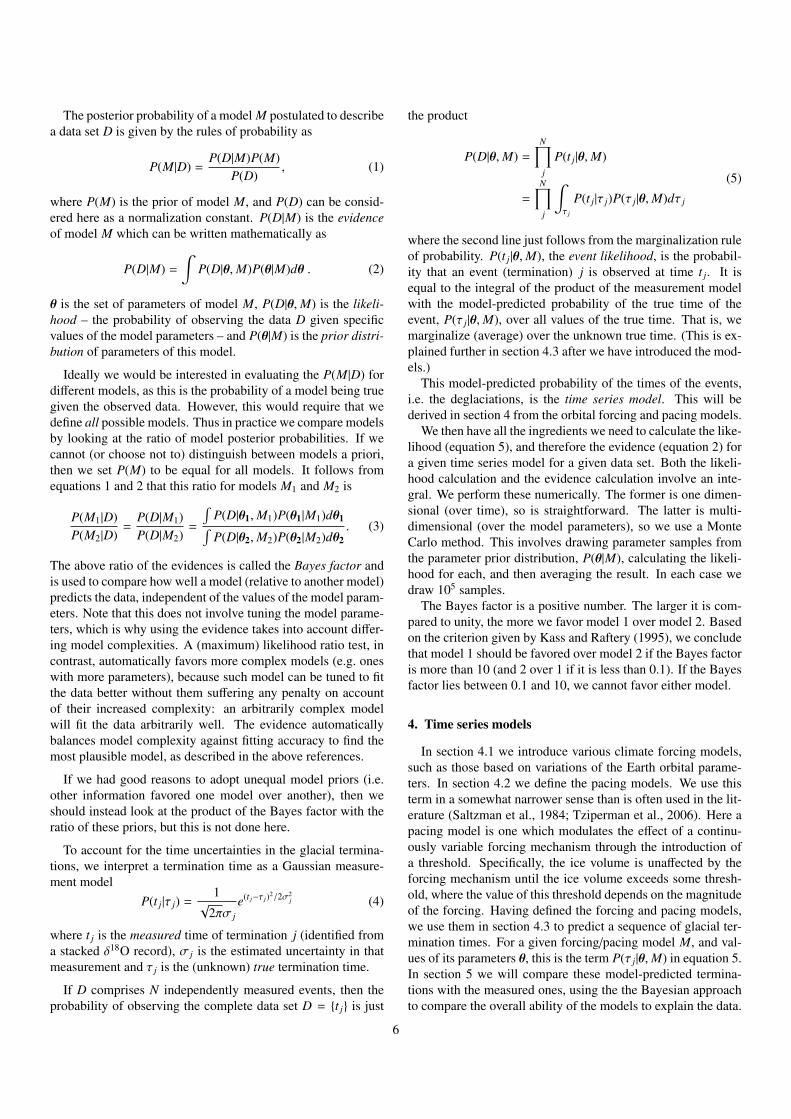
The posterior probability of a model M postulated to describea data set D is given by the rules of probability as

P(M|D) =P(D|M)P(M)

P(D), (1)

where P(M) is the prior of model M, and P(D) can be consid-ered here as a normalization constant. P(D|M) is the evidenceof model M which can be written mathematically as

P(D|M) =

∫P(D|θ,M)P(θ|M)dθ . (2)

θ is the set of parameters of model M, P(D|θ,M) is the likeli-hood – the probability of observing the data D given specificvalues of the model parameters – and P(θ|M) is the prior distri-bution of parameters of this model.

Ideally we would be interested in evaluating the P(M|D) fordifferent models, as this is the probability of a model being truegiven the observed data. However, this would require that wedefine all possible models. Thus in practice we compare modelsby looking at the ratio of model posterior probabilities. If wecannot (or choose not to) distinguish between models a priori,then we set P(M) to be equal for all models. It follows fromequations 1 and 2 that this ratio for models M1 and M2 is

P(M1|D)P(M2|D)

=P(D|M1)P(D|M2)

=

∫P(D|θ1,M1)P(θ1|M1)dθ1∫P(D|θ2,M2)P(θ2|M2)dθ2

. (3)

The above ratio of the evidences is called the Bayes factor andis used to compare how well a model (relative to another model)predicts the data, independent of the values of the model param-eters. Note that this does not involve tuning the model parame-ters, which is why using the evidence takes into account differ-ing model complexities. A (maximum) likelihood ratio test, incontrast, automatically favors more complex models (e.g. oneswith more parameters), because such model can be tuned to fitthe data better without them suffering any penalty on accountof their increased complexity: an arbitrarily complex modelwill fit the data arbitrarily well. The evidence automaticallybalances model complexity against fitting accuracy to find themost plausible model, as described in the above references.

If we had good reasons to adopt unequal model priors (i.e.other information favored one model over another), then weshould instead look at the product of the Bayes factor with theratio of these priors, but this is not done here.

To account for the time uncertainties in the glacial termina-tions, we interpret a termination time as a Gaussian measure-ment model

P(t j|τ j) =1

√2πσ j

e(t j−τ j)2/2σ2j (4)

where t j is the measured time of termination j (identified froma stacked δ18O record), σ j is the estimated uncertainty in thatmeasurement and τ j is the (unknown) true termination time.

If D comprises N independently measured events, then theprobability of observing the complete data set D = {t j} is just

the product

P(D|θ,M) =

N∏j

P(t j|θ,M)

=

N∏j

∫τ j

P(t j|τ j)P(τ j|θ,M)dτ j

(5)

where the second line just follows from the marginalization ruleof probability. P(t j|θ,M), the event likelihood, is the probabil-ity that an event (termination) j is observed at time t j. It isequal to the integral of the product of the measurement modelwith the model-predicted probability of the true time of theevent, P(τ j|θ,M), over all values of the true time. That is, wemarginalize (average) over the unknown true time. (This is ex-plained further in section 4.3 after we have introduced the mod-els.)

This model-predicted probability of the times of the events,i.e. the deglaciations, is the time series model. This will bederived in section 4 from the orbital forcing and pacing models.

We then have all the ingredients we need to calculate the like-lihood (equation 5), and therefore the evidence (equation 2) fora given time series model for a given data set. Both the likeli-hood calculation and the evidence calculation involve an inte-gral. We perform these numerically. The former is one dimen-sional (over time), so is straightforward. The latter is multi-dimensional (over the model parameters), so we use a MonteCarlo method. This involves drawing parameter samples fromthe parameter prior distribution, P(θ|M), calculating the likeli-hood for each, and then averaging the result. In each case wedraw 105 samples.

The Bayes factor is a positive number. The larger it is com-pared to unity, the more we favor model 1 over model 2. Basedon the criterion given by Kass and Raftery (1995), we concludethat model 1 should be favored over model 2 if the Bayes factoris more than 10 (and 2 over 1 if it is less than 0.1). If the Bayesfactor lies between 0.1 and 10, we cannot favor either model.

4. Time series models

In section 4.1 we introduce various climate forcing models,such as those based on variations of the Earth orbital parame-ters. In section 4.2 we define the pacing models. We use thisterm in a somewhat narrower sense than is often used in the lit-erature (Saltzman et al., 1984; Tziperman et al., 2006). Here apacing model is one which modulates the effect of a continu-ously variable forcing mechanism through the introduction ofa threshold. Specifically, the ice volume is unaffected by theforcing mechanism until the ice volume exceeds some thresh-old, where the value of this threshold depends on the magnitudeof the forcing. Having defined the forcing and pacing models,we use them in section 4.3 to predict a sequence of glacial ter-mination times. For a given forcing/pacing model M, and val-ues of its parameters θ, this is the term P(τ j|θ,M) in equation 5.In section 5 we will compare these model-predicted termina-tions with the measured ones, using the the Bayesian approachto compare the overall ability of the models to explain the data.

6

4.1. Forcing models

Insolation influences the climate in a number of ways, bothdirectly through mechanisms such as heating the lower atmo-sphere, and indirectly through modifying the ice accumula-tion rate and other mechanisms (Berger, 1978b,a; Saltzman andMaasch, 1990). Mainstream thinking holds that climate changeis most sensitive to the northern summer insolation at high lat-itudes because the temperature in continental areas, of whichthere is more in the northern hemisphere, is critical for ice melt-ing or sublimation (Milankovic, 1941). The summer insolationat high latitudes depends on the geometry of the Earth’s orbitand the inclination of Earth’s spin axis, and thus depends onthe eccentricity, precession, and obliquity (hereafter referred tocollectively as “orbital elements”, even though obliquity is notorbital). Variations in these alter how the insolation varies withseason (from orbital and axial precession), with latitude (fromobliquity changes), and with time scale (e.g. eccentricity varia-tions occur at dominant periods of 100 kyr and 400 kyr).

Milankovitch proposed that the combination of orbital ele-ments which gives rise to the measured summer insolation at65◦N is crucial to generating the glacial-interglacial cycles (Mi-lankovic, 1941; Hays et al., 1976). To model orbital forcingsmore generally, we define an orbital forcing model, f (t), as acombination of eccentricity, precession, and obliquity, which isproportional to the insolation over certain time scales, seasons,and latitudes. We build the following forcing models based onthe reconstructed time-varying eccentricity, fE(t), precession,fP(t), obliquity, fT(t), and four different combinations thereof:

fE(t) = e(t)fP(t) = e(t) sin(ω(t) − φ)fT(t) = ε(t)

fEP(t) = α1/2 fE(t) + (1 − α)1/2 fP(t)

fET(t) = α1/2 fE(t) + (1 − α)1/2 fT(t)

fPT(t) = α1/2 fP(t) + (1 − α)1/2 fT(t)

fEPT(t) = α1/2 fE(t) + β1/2 fP(t) + (1 − α − β)1/2 fT(t),

(6)

where e(t), ε(t), and e(t) sin(ω(t)−φ) are the eccentricity, obliq-uity, and precession index (or climatic precession), respectively.ω(t) is the angle between perihelion and the vernal equinox, andφ is a parameter controlling the phase of the precession. Weuse the variations of these three orbital elements over the past2 Myr as calculated by Laskar et al. (2004). We standardizeeach of fE(t), fP(t), and fT (t) to have zero mean and unit vari-ance, and then combine them to generate the compound mod-els. α and β are contribution factors which determine the rela-tive contribution of each component in the compound models,where 0 ≤ α ≤ 1 and 0 ≤ β ≤ 1. In addition to these models,we also use the daily-averaged insolation at 65◦N on July 21 asa proxy for the Milankovitch forcing, fCMF.

Beyond orbital forcings, we also consider the influence ofvariations of the Earth’s orbital inclination and of the cosmicray flux. To do this we build an inclination-based forcingmodel, fInc(t), using the orbital inclination calculated by Mullerand MacDonald (1997), and we model the cosmic ray forcing

as a geomagnetic paleointensity (GPI) time series (standardizedto the mean and unit variance), fG(t), as collected by Channellet al. (2009).

All forcing models and corresponding prior distributionsover their parameters (“forcing parameters”) are shown in Ta-ble 2. In this table and the following sections, all parametersare treated as dimensionless variables by setting the time unitto be 1 kyr (ice volume is on a relative scale). For the preces-sion model, we set φ = 0 to treat precession according to theMilankovitch theory (although in section 6 we will allow thephase of the precession to vary in order to check the sensitivityof our results to this assumption). As we do not have any priorinformation about the values of the contribution factors in thecompound models, we adopt uniform prior distributions overthe interval [0, 1] for these.

Figure 3 shows the single-component forcing models (whichdo not have any adjustable parameters). All forcing models willbe included in pacing models and corresponding terminationmodels in the following sections. Hereafter, for each forcingmodel, the corresponding pacing and termination models sharethe same name as shown in the first column of Table 2.

4.2. Pacing models

As described earlier, we use the term “pacing” to mean thatsome aspect of the climate system is independent of externalforcings until the climate system reaches a threshold, wherebythe value of this threshold is dependent upon the forcing. Wemodel the pacing effect on ice volume variations using the de-terministic version of the stochastic model introduced by Huy-bers and Wunsch (2005). In that model the ice volume at time tis

v(t) = v(t−∆t)+η(t) and if v(t) > h(t) then terminate, (7)

whereh(t) = h0 − a f (t), (8)

and ∆t is a constant time interval. Thus the ice volume changesin discrete steps until it passes a threshold h(t), which is itselfmodulated by a climate forcing f (t) with a contribution factora. The initial ice volume is v0 and the background threshold,h0, is either a constant or can itself vary with time. We setη(t) to be unity while the threshold has not been reached; af-ter that the glaciation is terminated by setting η(t) to a constantnegative value such that the ice volume linearly decreases to0 within 10 kyr of the threshold having been exceeded.3 Afterthis η(t) is set to unity, the next cycle starts. The threshold andthe deglaciation duration are chosen to generate approximately100 and 41 kyr glacial cycles (Huybers and Wunsch, 2005). Ifthe contribution factor a is zero, the ice volume will vary witha period modulated by the background threshold, h0. We de-fine this model as the Periodic model. In general the periodmay vary with time. However, if h0 is constant, then the Peri-odic model has a constant period of value h0 + 10 kyr. Because

3In practice the ice volume can go slightly negative due to the finite valueof ∆t, but this is of no practical consequence.

7

Table 2: The termination models and corresponding forcing models and parameters. In addition to any forcing model parameterslisted, the termination models have pacing parameters and the background fraction parameter. The prior distributions of theseparameters are described in sections 4.1, 4.2, and 4.3, respectively.

Termination Description Forcing Forcing modelmodel model parametersPeriodic 100 kyr pure periodic model None —Eccentricity Eccentricity fE(t) —Precession Precession fP(t) φTilt Tilt or obliquity fT(t) —EP Eccentricity plus Precession fEP(t) α, φET Eccentricity plus Tilt fET(t) αPT Precession plus Tilt fPT(t) α, φEPT Eccentricity plus Precession plus Tilt fEPT(t) α, β, φCMF (Classical) Milankovitch forcing fCMF(t) —Inclination Inclination fInc(t) —GPI Geomagnetic paleointensity fG(t) —

Time/kyr

Nor

mal

ized

forc

ing

mod

els

−2000 −1500 −1000 −500 0

−101

−101

−101

−101

−101

−101

Eccentricity

Precession

Tilt

CMF

Inclination

GPI

Figure 3: The single-component forcing models. A deglaciation is likely to be triggered by a peak in the forcing. The values ofeccentricity, precession, obliquity and Milankovitch forcing (CMF) are calculated by Laskar et al. (2004), the orbital inclinationrelative to the invariable plane is given by Muller and MacDonald (1997), and the GPI record is from Channell et al. (2009).

h0 controls the period of ice volume variations, different val-ues of h0 are required to model the 100 kyr cycles in the latePleistocene and the 41 kyr cycles in the early Pleistocene (seeFigure 4). We therefore first build pacing models to separatelypredict the deglaciations over the early and late Pleistocene us-ing the constant background threshold model. We then use avarying background threshold (either linear or sigmoidal) to tryto model the whole Pleistocene. We now describe these modelsin more detail.

4.2.1. Constant background threshold

A constant background threshold is appropriate for modelingglacial-interglacial cycles without a transition such as the MPT.One realization of such a pacing model with the threshold mod-ulated by a PT forcing model is shown in Figure 5. The ice vol-ume grows until it passes the forcing-modulated threshold. Theice volume then decreases rapidly to zero within the next 10 kyr.We see that a deglaciation tends to occur when the insolation isnear a local maximum. Hence the pacing model (equations 7and 8) can generate ∼100 kyr saw-tooth cycles which enables aforcing mechanism to pace the phase of these cycles.

The pacing model has three parameters: v0, h0, a. Rather

8

−2000 −1500 −1000 −500 0

Time/kyr

Ice

volu

me/

Arb

itrar

y un

its

030

6090

Constant threshold: h0=30 if t>−1000,h0=90 otherwise

Linear threshold: p=0.03, q=110

Sigmoid threshold: k=110, τ=200, t0=−1000

Sigmoid threshold: k=110, τ=100, t0=−1000

Sigmoid threshold: k=110, τ=200, t0=−800

Figure 4: Effect of the threshold in the pacing model. Different values of the threshold, h0(t), are shown: constant (red), linear(green), sigmoidal (blue, cyan, black). The legend shows the values of the parameters of the linear and sigmoid backgroundthresholds according to equations 9 and 10 respectively. The Periodic model is achieved using a constant threshold over some timespan. By changing it from h0 = 30 in the early Pleistocene to h0 = 90 in the late Pleistocene, we can reproduce an abrupt change inthe period of ice volume variations from ∼41 kyr to ∼100 kyr.

−1000 −800 −600 −400 −200 0

050

100

150

Time/kyr

Ice

volu

me/

Arb

itrar

y un

its

Figure 5: A pacing model with threshold h(t) modulated by the PT forcing model with α = 0.5 and φ = 0 (equation 6). Thepacing model parameters are: background threshold h0 = 90; initial ice volume v0 = 25; contribution factor of forcing a = 25.The dashed line denotes the constant threshold, and the grey line represents the threshold modulated by the PT forcing model, i.e.h(t) = h0 − a fPT(t;α = 0.5, φ = 0).

than fixing these to some expected values, we assign a proba-bility distribution to them. This is the prior which appears inequation 2, which shows that by averaging the likelihood overvalues drawn from this prior we get the evidence for the model.

As described above, a periodic pacing model is generated byadopting a constant threshold, h(t) = h0 and a = 0. Whenforcings are added onto the constant threshold (to give a , 0),the ice volume variations then have an average period of about(h0 + 10−a) kyr, because ice volume accumulation tends to ter-

minate at a forcing maxima. For this reason we use differentprior distributions on a and h0 depending on whether we aretrying to model the early (41 kyr cycles) or late (100 kyr cycles)Pleistocene. Specifically, we use prior distributions for v0, h0,and a which are uniform over the following intervals (and zerooutside): 0 < v0 < 90γ, 90γ < h0 < 130γ, 15γ < a < 35γ,where γ = 0.4 when we model ∼41 kyr cycles and γ = 1 whenwe model ∼100 kyr cycles. The range of v0 is just the range ofthe ice volume variation, while the mean values of the prior dis-

9

tributions of h0 and a with γ = 1 are the fitted values obtainedby Huybers (2011). For the periodic model, a is zero and h0 hasa uniform prior distribution over 70γ < h0 < 110γ. In section6, we will check how sensitive our results are to this choice ofpriors.

4.2.2. Linear trend background thresholdThe constant background threshold model is incapable of

modeling the transition from the 41 kyr world to the 100 kyrworld. If we treat h0 as a step function as shown in Figure 4(red lines), the corresponding pacing model predicts an abruptMPT with an extra parameter (the time of the transition). Butto model the MPT, we will introduce another two versions ofthe pacing model by allowing the background threshold to varywith time (linearly and nonlinearly).

Studies have suggested various mechanisms which may beinvolved in climate change before and after the MPT (Saltzmanet al., 1984; Maasch and Saltzman, 1990; Ghil, 1994; Raymoet al., 1997; Paillard, 1998; Clark et al., 1999; Tziperman andGildor, 2003; Ashkenazy and Tziperman, 2004). H07 suggeststhat a simple model with a threshold modulated by obliquityand a linear trend can explain changes in glacial variability overthe last 2 Myr without invoking complex mechanisms. To in-vestigate this, we replace the threshold constant h0 with a lineartrend in time

h0 = pt + q, (9)

where p and q are the slope and intercept of the trend respec-tively. To predict the transition from 41 kyr cycles to 100 kyr cy-cles with reasonable parameter sets, we adopt the following uni-form prior distributions for the pacing parameters: 0 < v0 < 36,0 < p < 0.1, 106 < q < 146 and 10 < a < 30. For the Periodicmodel we use a = 0 and a uniform prior for q between 86 and126. These ranges are adopted so that the pacing model predictsthe 41 kyr and 100 kyr cycles with similar period uncertaintiesas produced by the ranges of parameters in the pacing modelwith a constant background threshold (section 4.2.1).

An example of the linear trend is shown with the green line inFigure 4. If the threshold is not modulated by any forcing (i.e.a = 0, the Periodic model), then the pacing model generates agradual transition from 50 kyr cycles 2 Ma to 110 kyr cycles atthe present.

4.2.3. Sigmoid trend background thresholdTo enable a more rapid onset of the MPT, we introduce an-

other version of the pacing model with a nonlinear trend in thebackground threshold, defined using the sigmoid function as

h0 = 0.6k/(1 + e−(t−t0)/τ) + 0.4k, (10)

where k is a scaling factor, t0 denotes the transition time, andτ represents the time scale of the MPT. The uniform priors ofthe parameters of this version of pacing models are set to be:0 < v0 < 36, 90 < k < 130, 10 < τ < 500, 10 < a < 30,and −700 < t0 < −1250, as motivated by the range of MPTtime given by Clark et al. (2006). For the Periodic model weset a = 0 and change the range of k to be 70 < k < 110. The

reason for choosing these priors is the same as given in section4.2.2.

Figure 4 illustrates this model. A late transition time, t0,moves the trend to the present, and a smaller transition timescale, τ, generates a more rapid transition. The values of 0.6kand 0.4k in the above equation are set in order to rescale thetrend model such that the ice volume threshold including a sig-moid trend allows both ∼41 kyr and ∼100 kyr ice volume vari-ations.

4.3. Termination models

Using the same method described in section 2 for the data,we identify glacial terminations in the ice volume time seriesgenerated by the pacing models. The age uncertainty of eachtermination is equal to half of the duration of the termination.As with the data, a single termination is represented as a Gaus-sian probability distribution over time, which is just the termP(τ j|θ,M) in equation 5 (see section 3). The full set of pre-dicted terminations forms the time series model which we willcompare with the data. We use the term “termination model” torefer to the combination of a forcing model and a pacing model,which together has a number of parameters. These are listed inTable 2. Each of these termination models can have differentbackground threshold models, as was explained in section 4.2.

Figure 6 shows schematically how we compare the model-derived terminations (red line) with the data on one termination(black line). The event likelihood (the integral in equation 5) fora termination is calculated by integrating over time the productof the probability distribution of the observed time of the ter-mination, P(t j|σ j, τ j), with the model prediction of the true ter-mination time, P(τ j|θ,M). The product of event likelihoods forall terminations in a data set is the likelihood for the termina-tion model with specific values of the parameters of the forcingand pacing model. By calculating the likelihood for many dif-ferent values of those parameters (drawn from their prior distri-butions), and averaging them, we arrive at the evidence for thattermination model (equation 2).

To accommodate other contributions from the climate systemto the timing of a termination, we add a constant backgroundprobability to the termination model. This is defined using thebackground fraction b = Hb/(Hb + Hg), where Hb is the am-plitude of the background and Hg is the difference between themaximum and minimum of the Gaussian sequence. The back-ground fraction is a parameter of the model which we do notmeasure, so we assign it a prior (uniform from 0 to 0.1) andmarginalize over this too.

Let us summarize our modelling procedure. A forcing model(Figure 3) modulates the ice volume threshold (equation 8)of the pacing model (equation 7) from which the terminationmodel (e.g. red line in Figure 6) is derived. This is then com-pared with a sequence of terminations identified from a δ18Odata set using our Bayesian procedure.

10

−1000 −800 −600 −400 −200 0

Time/kyr

P(τj|θ,M)P(tj|σj,τj)

Figure 6: Schematic illustration of the components in the likelihood calculation (equation 5). The red line is the termination modelgenerated from the pacing model shown in Figure 5. The black line represents the measured data on termination j. Its time anduncertainty are interpreted probabilistically as a Gaussian distribution over time.

5. Results of the model comparison

5.1. Evidence and Bayes factorWe calculate the Bayesian evidence of the termination mod-

els listed in Table 2 for each of the data sets shown in Table 1.We calculate this for terminations extending over three differenttime spans: 1 Ma to 0 Ma, 2 Ma to 1 Ma and 2 Ma to 0 Ma. Thefirst time span is the same as that chosen by Huybers (2011).However, other studies claim that the onset of 100 kyr cyclesoccurred around 0.8 Ma. We will examine in section 6 howsensitive our results are to the choice of time span. Accordingto the time span in question, we need to choose the appropriatepacing model, because this determines the dominant period.

The Bayes factor (BF) is just the ratio of the evidence for twomodels. Rather than reporting Bayes factors for various pairs ofmodels, we will report them for all models relative to a simplereference termination model. This reference model is just a uni-form probability distribution over the time of deglaciations, andhas no parameters. It corresponds to a constant probability intime of a deglaciation, but its choice is arbitrary as it just servesto put the evidences on a convenient scale.

Bayes factors should only be used to compare different mod-els for a common data set. This is because their definition re-quires that the factor P(D) in equation 3 cancels out.

5.1.1. Late Pleistocene (1-0 Ma)The deglaciations identified using H07’s method (in the data

sets HA, HB, HP, LR04, and LRH) contain many minor termi-nations which may be better explained by models which predict∼41 kyr cycles. Thus, we choose constant background thresh-olds with γ = 1 and γ = 0.4 for all termination models in orderto predict 100 kyr and 41 kyr variations, respectively, over thepast 1 Myr.

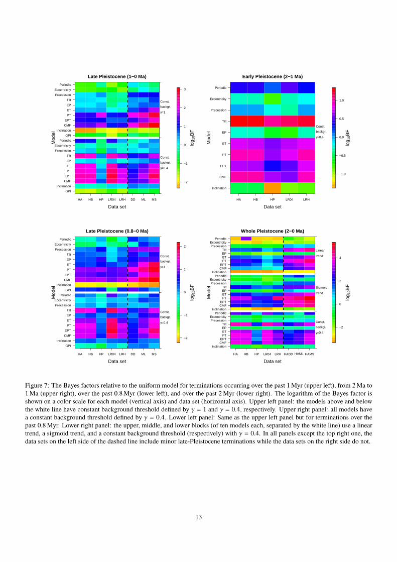
The BF for each termination model relative to the uniformmodel is shown in Figure 7. We see that the HA, HB, LR04,and LRH data sets favor the models with a tilt component andwith γ = 0.4. Although compound models such as EPT and

CMF sometimes have BFs slightly higher than the Tilt model,precession and eccentricity may not be necessary to explain theterminations identified in these data sets.

The HP data set favors the PT model with γ = 1. This couldbe caused by a mismatch between the terminations identifiedin HP and the terminations identified in other data sets. Forexample, around the time of termination 6 (Figure 2), two ter-minations are identified in HP while only one termination isidentified in other data sets. The discrepancy between HP andother data sets is larger before 0.8 Ma, which indicates a moreambiguous definition of terminations, particularly for plankticδ18O. On account of this, in section 6 we will narrow the timespan to 0-0.8 Ma (a more conservative time scale of late Pleis-tocene). Nevertheless, for all the data sets containing minorterminations, tilt is a common factor in the preferred models.

For the DD, ML, and MS data sets, the PT and CMF modelswith γ = 1 are favored. In other words, the major terminationsare better predicted by a model involving precession and tiltrather than either alone, although tilt alone can pace minor ter-minations. Because the EPT and CMF models have lower BFsthan the PT model, the eccentricity component is unlikely topace the glacial terminations directly. Yet eccentricity can de-termine the glacial terminations indirectly through modulatingthe amplitude of the precession maxima (i.e. e sinω). A similarconclusion was drawn by Huybers (2011) using p-values. Wenote that the rejection of a null hypothesis in this way does notautomatically validate the alternative hypothesis. The Bayesianapproach allows one to directly compare multiple models in asymmetric fashion.

Since the late Pleistocene is characterized predominantly bymajor terminations, we conclude that late Pleistocene climatechange is paced by a combination of obliquity and preces-sion. This does not automatically imply that there is no linkbetween major terminations and eccentricity variations. Eccen-tricity may determine the 100 kyr cycles in the late Pleistocene,while obliquity and precession influence the exact timing of theterminations (Lisiecki, 2010). This could be studied in future

11

work by introducing an eccentricity dependence into the pacingmodel.

5.1.2. Early Pleistocene (2-1 Ma)Here we only consider the HA, HP, HB, L04, and LRH data

sets, because the DD, ML, and MS sets have no terminations inthe early Pleistocene. We only calculate BFs for models withγ = 0.4 (and not γ = 1), because this reproduces periods onthe order of 41 kyr, and such cycles are obvious in all data sets(Figure 2). We exclude the GPI model because the GPI recordhas a time span less than 2 Myr. The BFs for the terminationmodels are shown in the upper right panel of Figure 7.

We see that the Tilt model is favored by all data sets. Thecombination of tilt with other orbital elements does not give ahigher BF, so we conclude that the other orbital elements donot play a major role in pacing the deglaciations over the earlyPleistocene. It is important to realise that although the Bayesianevidence generally penalizes more complex models, this doesnot automatically result in a lower Bayes factor for such mod-els. They can achieve higher Bayes factors if the model is sup-ported by the data sufficiently strongly (see the references insection 3).

5.1.3. Whole Pleistocene (2-0 Ma)For the whole Pleistocene we use the data sets HA, HB, HP,

LR04, and LRH as well as the hybrid data sets, HADD, HAML,and HAMS. We use pacing models with and without a trendthreshold to model the terminations. The BFs for the abovemodels and data sets are shown in the lower left panel of Figure7.

For the HA, HB, and LR04 data sets, the Tilt model withγ = 0.4 is favored. Other combinations with the tilt componentand with γ = 0.4 yield similar BFs. However, for the HP andLRH data sets, the PT model with a sigmoid trend is favoredand this model also gives high BFs for the HA, HB, and LR04data sets. For all these data sets, the Precession, Eccentricity,and Periodic models have rather low BFs. These results indicatea major role for tilt and a minor role for precession in pacingmajor and minor Pleistocene deglaciations. For all the abovedata sets, the CMF model with γ = 0.4 has a high BF, butnot higher than other models with a tilt component. CMF isan optimized version of the EPT model. Faced with differentmodels which give similar Bayes factors, we will normally wantto choose the simplest, which here is PT. We will investigatethis further in section 6.

For the HADD, HAML, and HAMS data sets, the PT modelwith a threshold modulated by a sigmoid trend is favored, andthose compound models with a tilt component also have highBFs. The whole Pleistocene deglaciations appear to be pacedby the combination of precession and obliquity. This is con-sistent with the results for the late-Pleistocene deglaciations.The physical reason why precession becomes important afterthe MPT is beyond the scope of our work and is still under de-bate.

On account of the existence of the MPT, modeling the wholePleistocene with a constant background threshold model makeslittle sense, so those corresponding results should not be given

much weight. (This corresponds to assigning all those modelsa smaller model prior, P(M).) More appropriate are the modelswith linear and sigmoid background thresholds. Among these,we see that the EPT and CMF models have BFs about ten timeslower than the PT model. We conclude that eccentricity doesnot play a significant role in pacing terminations over the wholePleistocene. We also find that the PT model with a sigmoidbackground threshold is more favored than the PT model witha linear background threshold, which indicates that the MPTmay not be as gradual as claimed by (Huybers, 2007). We willdiscuss this further in section 6.

According to Figure 7, the Inclination and GPI models arenot favored, and in fact are less favored than the reference uni-form model (as BF<1). Thus we find that the geomagnetic pa-leointensity does not pace glacial cycles over the last 2 Myr, al-though we note that there is some controversy over the link be-tween the GPI and climate change (Courtillot et al., 2007; Pier-rehumbert, 2008; Bard and Delaygue, 2008; Courtillot et al.,2008). In contrast to the conclusion of Muller and MacDonald(1997), there we find no evidence for a link between the orbitalinclination and ice volume change.

5.2. Discrimination powerTo validate our method as an effective inference tool to select

out the true model, we generate simulated data from each modeland then evaluate the Bayes factors for all models on these data.The data are simulated with the following parameters for allmodels except the Periodic one: h0 = 110γ, a = 25γ, b = 0,and v0 = 45γ, where γ = 1 for terminations simulated overthe last 1 Myr and γ = 0.4 for the time range 2 to 1 Ma. Forthe Periodic model we use instead of h0 = 90γ and of coursea = 0. Recall that the period of the resulting time series isapproximately h0 + 10 − a. Other parameters in correspondingforcing models are fixed at α = 0.5 for compound models withtwo components, α = 0.3 and β = 0.2 for the EPT model, andφ = 0 for models with a precession component.

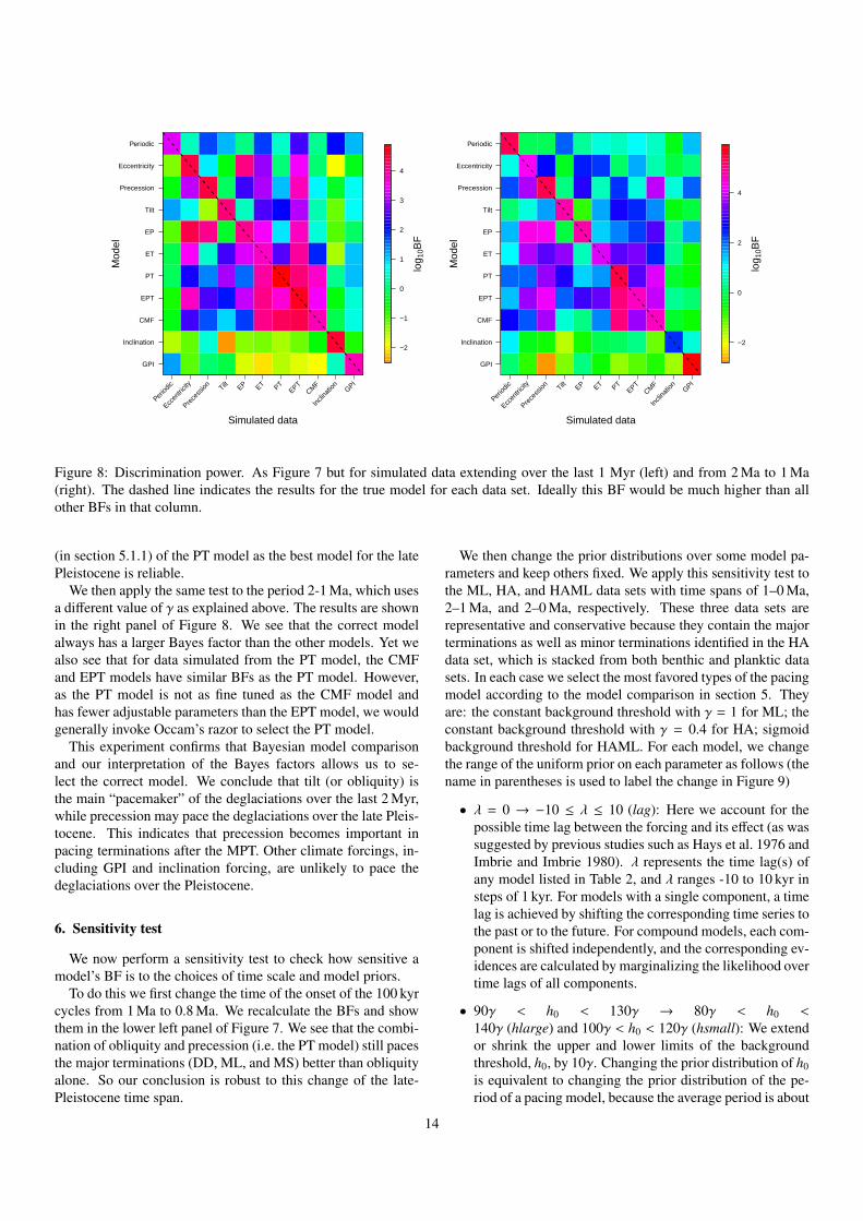
The BFs for simulated data over the last 1 Myr are shownin the left panel of Figure 8. We see that all models based ona single orbital element are correctly selected, although thosemodels combining the correct single orbital element with otherelements may also give comparable BFs. When models havesimilar BFs we would generally want to favor the one withfewest components. This again corresponds to using a largervalue of the model prior, P(M) (see section 3).

Incorrect models, in contrast, generally receive much lowerBayes factors. For the PT-simulated data set, the PT modelis correctly discriminated from the CMF model (a fitted EPTmodel). We also see that although the ET model may not becorrectly selected out when its BF is similar to that obtained forEP, PT, EPT, and CMF models, the ratios of the Bayes factorsare close to unity. The much larger ratios between them for thereal data validate our inference of the ET model (see section 5).Figure 8 shows that the EP model is not favored over the Eccen-tricity model even when the former is the true model. However,the Eccentricity model is never favored on any of the real datasets, so this misidentification does not occur in practice. In con-clusion, this discrimination test indicates that our identification

12

Late Pleistocene (1−0 Ma)

Mod

el

HA HB HP LR04 LRH DD ML MS

Data set

GPI

Inclination

CMF

EPT

PT

ET

EP

Tilt

Precession

Eccentricity

Periodic

GPI

Inclination

CMF

EPT

PT

ET

EP

Tilt

Precession

Eccentricity

Periodic

Const.

backgr.

γ=1

Const.

backgr.

γ=0.4

−2

−1

0

1

2

3

log 1

0BF

Early Pleistocene (2−1 Ma)

Mod

el

HA HB HP LR04 LRH

Data set

Inclination

CMF

EPT

PT

ET

EP

Tilt

Precession

Eccentricity

Periodic

Const.

backgr.

γ=0.4

−1.0

−0.5

0.0

0.5

1.0

log 1

0BF

Late Pleistocene (0.8−0 Ma)

Mod

el

HA HB HP LR04 LRH DD ML MS

Data set

GPI

Inclination

CMF

EPT

PT

ET

EP

Tilt

Precession

Eccentricity

Periodic

GPI

Inclination

CMF

EPT

PT

ET

EP

Tilt

Precession

Eccentricity

Periodic

Const.

backgr.

γ=1

Const.

backgr.

γ=0.4

−2

−1

0

1

2

log 1

0BF

Whole Pleistocene (2−0 Ma)

Mod

el

HA HB HP LR04 LRH HADD HAMS

Data set

HAML

InclinationCMFEPT

PTETEPTilt

PrecessionEccentricity

PeriodicInclination

CMFEPT

PTETEPTilt

PrecessionEccentricity

PeriodicInclination

CMFEPT

PTETEPTilt

PrecessionEccentricity

Periodic

Linear

trend

Sigmoid

trend

Const.

backgr.

γ=0.4

−2

0

2

4

log 1

0BF

Figure 7: The Bayes factors relative to the uniform model for terminations occurring over the past 1 Myr (upper left), from 2 Ma to1 Ma (upper right), over the past 0.8 Myr (lower left), and over the past 2 Myr (lower right). The logarithm of the Bayes factor isshown on a color scale for each model (vertical axis) and data set (horizontal axis). Upper left panel: the models above and belowthe white line have constant background threshold defined by γ = 1 and γ = 0.4, respectively. Upper right panel: all models havea constant background threshold defined by γ = 0.4. Lower left panel: Same as the upper left panel but for terminations over thepast 0.8 Myr. Lower right panel: the upper, middle, and lower blocks (of ten models each, separated by the white line) use a lineartrend, a sigmoid trend, and a constant background threshold (respectively) with γ = 0.4. In all panels except the top right one, thedata sets on the left side of the dashed line include minor late-Pleistocene terminations while the data sets on the right side do not.

13

Simulated data

Mod

el

Period

ic

Eccen

tricit

y

Prece

ssion Tilt EP ET PT

EPTCM

F

Incli

natio

nGPI

GPI

Inclination

CMF

EPT

PT

ET

EP

Tilt

Precession

Eccentricity

Periodic

−2

−1

0

1

2

3

4

log 1

0BF

Simulated data

Mod

el

Period

ic

Eccen

tricit

y

Prece

ssion Tilt EP ET PT

EPTCM

F

Incli

natio

nGPI

GPI

Inclination

CMF

EPT

PT

ET

EP

Tilt

Precession

Eccentricity

Periodic

−2

0

2

4

log 1

0BF

Figure 8: Discrimination power. As Figure 7 but for simulated data extending over the last 1 Myr (left) and from 2 Ma to 1 Ma(right). The dashed line indicates the results for the true model for each data set. Ideally this BF would be much higher than allother BFs in that column.

(in section 5.1.1) of the PT model as the best model for the latePleistocene is reliable.

We then apply the same test to the period 2-1 Ma, which usesa different value of γ as explained above. The results are shownin the right panel of Figure 8. We see that the correct modelalways has a larger Bayes factor than the other models. Yet wealso see that for data simulated from the PT model, the CMFand EPT models have similar BFs as the PT model. However,as the PT model is not as fine tuned as the CMF model andhas fewer adjustable parameters than the EPT model, we wouldgenerally invoke Occam’s razor to select the PT model.

This experiment confirms that Bayesian model comparisonand our interpretation of the Bayes factors allows us to se-lect the correct model. We conclude that tilt (or obliquity) isthe main “pacemaker” of the deglaciations over the last 2 Myr,while precession may pace the deglaciations over the late Pleis-tocene. This indicates that precession becomes important inpacing terminations after the MPT. Other climate forcings, in-cluding GPI and inclination forcing, are unlikely to pace thedeglaciations over the Pleistocene.

6. Sensitivity test

We now perform a sensitivity test to check how sensitive amodel’s BF is to the choices of time scale and model priors.

To do this we first change the time of the onset of the 100 kyrcycles from 1 Ma to 0.8 Ma. We recalculate the BFs and showthem in the lower left panel of Figure 7. We see that the combi-nation of obliquity and precession (i.e. the PT model) still pacesthe major terminations (DD, ML, and MS) better than obliquityalone. So our conclusion is robust to this change of the late-Pleistocene time span.

We then change the prior distributions over some model pa-rameters and keep others fixed. We apply this sensitivity test tothe ML, HA, and HAML data sets with time spans of 1–0 Ma,2–1 Ma, and 2–0 Ma, respectively. These three data sets arerepresentative and conservative because they contain the majorterminations as well as minor terminations identified in the HAdata set, which is stacked from both benthic and planktic datasets. In each case we select the most favored types of the pacingmodel according to the model comparison in section 5. Theyare: the constant background threshold with γ = 1 for ML; theconstant background threshold with γ = 0.4 for HA; sigmoidbackground threshold for HAML. For each model, we changethe range of the uniform prior on each parameter as follows (thename in parentheses is used to label the change in Figure 9)

• λ = 0 → −10 ≤ λ ≤ 10 (lag): Here we account for thepossible time lag between the forcing and its effect (as wassuggested by previous studies such as Hays et al. 1976 andImbrie and Imbrie 1980). λ represents the time lag(s) ofany model listed in Table 2, and λ ranges -10 to 10 kyr insteps of 1 kyr. For models with a single component, a timelag is achieved by shifting the corresponding time series tothe past or to the future. For compound models, each com-ponent is shifted independently, and the corresponding ev-idences are calculated by marginalizing the likelihood overtime lags of all components.

• 90γ < h0 < 130γ → 80γ < h0 <140γ (hlarge) and 100γ < h0 < 120γ (hsmall): We extendor shrink the upper and lower limits of the backgroundthreshold, h0, by 10γ. Changing the prior distribution of h0is equivalent to changing the prior distribution of the pe-riod of a pacing model, because the average period is about

14

h0 +10−a (see section 4.2.1). The above changes only ap-ply to models with a , 0 while the prior distribution of thePeriodic model (a = 0) is changed from 70γ < h0 < 110γfirst to 60γ < h0 < 120γ and then to 80γ < h0 < 100γ.For models with a sigmoid trend, the prior distribution ofk is changed from 90 < k < 130 first to 80 < k < 140 andthen to 100 < k < 120.

• 15γ < a < 35γ → 5γ < a < 45γ (alarge) or 20γ < a <30γ (asmall): We extend or shrink the range of contribu-tion factor of forcing, a, around its mean. These changesdo not apply to the Periodic model, for which a = 0.

• 0 < b < 0.1 → 0 < b < 0.2 (blarge) or 0 < b < 0.05 (as-mall): We double or halve the upper limit of b, the contri-bution factor of the background in the termination model.

• φ = 0 → −π < φ < π (phi): We now allow any value forthe the phase of the precession, φ, which is related to theseason of the insolation that forces the climate change.

The BFs for the models with each of the above changes areshown Figure 9, separated into three blocks corresponding tothe different data sets, ML, HA, HAML. For the ML data set (1–0 Ma; top block), the PT and CMF models are favored over theTilt model for all changes in the priors. The PT and CMF mod-els without time lags are also favored over corresponding mod-els with lags. This indicates that the Tilt and Precession modelspace climate change without significant time lags. Over theearly Pleistocene (middle block), the Tilt model is marginallyfavored. The BFs of the EPT model vary a lot but are neverhigher than the Tilt model. For the HAML data set (2–0 Myr;bottom block), the model combining a sigmoid trend and thePT forcing is favored for all changed priors. Moreover, theBF for the PT model increases when shrinking the range ofthe background fraction, b. The relative lack of significanceof the background suggests a significant influence of obliquityand precession over the past 2 Myr.

To further investigate the role of precession in pacing themajor late-Pleistocene deglaciations, we marginalize the like-lihoods for the PT model over all its parameters except forthe contribution factor of precession contribution factor, α, andphase, φ. (Note that the evidence is the likelihood marginal-ized over all model parameters.) We do this for the ML dataover the last 1 Myr. The distribution of this marginalized likeli-hood (relative to the uniform model) is shown in the left panelof Figure 10. The highest values occur for phases rangingfrom −50◦ < φ < +50◦, indicating that the main pacemakerunder this model is either the intensity of the northern hemi-sphere summer insolation or the duration of the southern sum-mer (we cannot distinguish between these based on availabledata). While very small contribution factors, α < 0.1, arestrongly disfavored, the model is otherwise not very sensitiveto α. Since α determines the size of the contribution of pre-cession to the PT model (equation 6), this means that someprecession contribution is favored, but the exact amount is notwell constrained. This broad high likelihood range of α and φ

means that the pacing depends on the overall northern hemi-sphere summer insolation at a range of northern latitudes (orequivalently the duration of the southern summer) rather thanthat at a specific latitude and time in summer. This is consis-tent with Huybers 2011’s conclusion that “climate systems arethoroughly interconnected across temporal and spatial scales”.

We found in section 5.1.3 that the pacing model with a sig-moid background threshold model was favored when modelingthe whole Pleistocene. We now identify which parameters ofthat model are most favored by the data. To do this we calcu-late the marginalized likelihood (relative to the uniform model)for the PT model with a sigmoid background threshold as afunction of both the transition time scale, τ, and transition mid-point, t0, on the HAML data set (i.e. we marginalize over allother parameters): see the right panel of Figure 10. To explorethis more completely we have extended the upper limit of t0from -700 kyr to -300 kyr. The peak is at around τ = 100 kyr(about one glacial-interglacial cycle) and t0 = −715 kyr. To vi-sualize this transition, a sigmoid background model with thisvalue of τ is shown in Figure 4. Defining the transition dura-tion as the time taken for the ice volume to change from 25% to75% of its maximum value, τ = 100 kyr corresponds to a tran-sition duration of 220 kyr. This timescale for the MPT is con-sistent with the findings of Hönisch et al. (2009); Mudelsee andSchulz (1997); Tziperman and Gildor (2003); Martínez-Garciaet al. (2011). It is shorter (more abrupt transition) that foundby H07 and others (Raymo et al., 2004; Liu and Herbert, 2004;Medina-Elizalde and Lea, 2005; Blunier et al., 1998), althoughFigure 10 shows that longer time scales are not that improba-ble (but note that the likelihoods are shown on a logarithmicscale). The transition time of 715 kyr ago is somewhat laterthan the mid-point of the MPT of ∼-900 kyr identified by Clarket al. (2006) using a frequency spectrogram analysis. Yet ourdata/analysis permits a range of values, although we see thatthe region around -900 kyr is disfavored for low values of τ.Discrepancies from previous results could also arise from thefact that we use just termination data.

As a final sensitivity test, we change the sign of the contri-bution factor of forcing, a, to model possible anticorrelationsbetween forcing models and the data over the late Pleistocene.We find that this significantly reduces the BF for all favoredmodels, which shows that models with anticorrelations are apoor description of the data.

7. Summary and conclusions

Using likelihood-based model comparison, we find that acombination of obliquity (axial tilt) and precession is the mainpacemaker of the 12 major glacial terminations in the late Pleis-tocene. Obliquity alone can trigger minor terminations over thewhole Pleistocene. The obliquity and precession pace the Pleis-tocene terminations without significant time lags, and their pac-ing roles can be identified with high significance.

We confirm the dominant role of obliquity in pacing theglacial terminations over the early Pleistocene. In contrast tothe conclusion of H07, we find that a model with obliquityalone describes the major and minor Pleistocene deglaciations

15

Mod

el

none lag

hlarg

e

hsm

all

alarg

e

asm

all

blarg

e

bsm

all phi

Changed prior

InclinationCMFEPT

PTETEPTilt

PrecessionEccentricity

PeriodicInclination

CMFEPT

PTETEPTilt

PrecessionEccentricity

PeriodicGPI

InclinationCMFEPT

PTETEPTilt

PrecessionEccentricity

Periodic

1−0 Ma

data: ML

γ=1

2−1 Ma

data: HA

γ=0.4

2−0 Ma

data: HAML

Sigmoid−2

0

2

4

log 1

0BF

Figure 9: Sensitivity test. Bayes factors for several models with a change in the range of priors (compared to what was used insection 5.1 and Figure 7). These are shown for three different data sets (and time scales) in the three blocks separated by whitehorizontal lines. In each block the logarithm of the Bayes factor is show on a color scale for each model (vertical axis) and changein prior (horizontal axis). The first column – labeled ‘none’ – gives the BFs for models with the original priors for reference. Somemodels are not relevant for certain prior changes, so the corresponding slots are empty (white). The three blocks are as follows.Top: pacing model with a constant background threshold with γ = 1 for the ML data set (0–1 Ma). Middle: pacing model witha constant background threshold with γ = 0.4 for the HA data set (1–2 Ma). Bottom: pacing model with a sigmoid backgroundthreshold for the HAML data set (0–2 Ma).

0.2 0.4 0.6 0.8

−15

0−

5050

150

α

φ (d

eg)

−2

−1

0

1

2

3

4

log 1

0(R

ML)

+

−1200 −800 −400

100

300

500

t0 kyr

τky

r

0123456

log 1

0(R

ML)

+

Figure 10: The distribution of the logarithm of the marginalized likelihood relative to the uniform model, log10(RML), for the PTmodel as a function of two model parameters. The left panel shows the distribution over the precession contribution factor (α) andphase (φ) for the PT model with γ = 1 for the ML data set (the last 1 Myr). The right panel shows the distribution over the transitiontime (t0) and transition time scale (τ) for the PT model with a sigmoid background threshold for the HAML data set (the last 2 Myr).106 and 1.6× 106 sample points sampled in a 200× 200 grid were used to construct the left and right distributions respectively. Foreach panel, the most favored region is identified by applying a 25 × 25 grid to the distribution, and is denoted by a cross. Note thatthe scales saturate: likelihoods above or below the limits of the color bar are plotted using the extreme color.

(together) better than a model which combines obliquity with atrend in the background threshold. Thus obliquity is sufficientto explain at least the time of minor terminations before andafter the MPT, without reparameterizing the model as done byH07 and Raymo et al. (1997); Paillard (1998); Ashkenazy and

Tziperman (2004); Paillard and Parrenin (2004); Clark et al.(2006).

We observe that precession becomes important in pacing the∼100 kyr glacial-interglacial cycles after the MPT. Through thecomparison of models with a linear trend and models with a

16

sigmoid trend in the background threshold, we find that theglacial terminations over the whole Pleistocene can be pacedby a combination of precession, obliquity, and a sigmoid trendin the background threshold. Using marginalized likelihoods,we find that the MPT has a time scale (the time required for icevolume to grow from 25% to 75% of the maximum) of about220 kyr and a mid-point at around 715 kyr before the present.This is rather late compared with other studies (Clark et al.,2006), although our data/analysis supports a broad range of val-ues. Note that we do not assume the existence of a strict peri-odicity in the data, in contrast to some studies based on powerspectrum analyses. Since there is no significant change in thepower spectrum of the insolation before and after the MPT, theMPT must be caused by a rapid change of response of the cli-mate to the insolation, rather than by the insolation itself. Thisis consistent with previous studies (Paillard, 1998; Parrenin andPaillard, 2003; Ashkenazy and Tziperman, 2004; Clark et al.,2006).

We also find that geomagnetic forcing and forcing bychanges in the inclination of the Earth’s orbital plane are un-likely to cause significant climate change over the last 2 Myr.This weakens the suggestion that the Earth’s orbital inclinationrelative to the invariable plane influences the climate (Mullerand MacDonald, 1997). Our results also suggest that the mod-ulation of cosmic rays or solar activity by the Earth’s mag-netic field has at best a limited impact on climate change ontimescales between 10 kyr and 1 Myr, challenging the hypoth-esis that connects the geomagnetic paleointensity with climatechange (Channell et al., 2009).

The Bayesian modelling approach is well suited to multiplemodel comparison, because it evaluates all their evidences ex-plicitly: a model is not selected just because some alternative“noise” model is rejected. Uncertainties in the data are also ac-commodated. Moreover, the approach automatically and con-sistently takes into account the model complexity, in contrast tomost other methods (e.g. frequentist hypothesis testing, max-imum likelihood ratio tests) which will favor more complexmodels unless they are penalized in some ad hoc way.

Our conclusions are reasonably robust to changes of param-eters, priors, time scales, and data sets. The main uncertaintyin our work comes from the identification of glacial termina-tions over the Pleistocene, although we have used different datasets of terminations to reduce this uncertainty. In future work,a more sophisticated Bayesian method (e.g. the method intro-duced by Bailer-Jones 2012) could be employed to model thefull time series of climate proxies. Using this model inferenceapproach, we may learn more about the mechanisms involvedin the climate response to Milankovitch forcings.

Acknowledgements

We thank Joerg Lippold for pointing us to relevant litera-ture, Marcus Christl for providing 10Be data, and Martin Frankfor explaining the method of reconstructing the history of so-lar activity. Morgan Fouesneau, Eric Gaidos, and Gregor Sei-del gave valuable comments on the manuscript. We also thankanonymous referee and the associate editor, Michel Crucifix,

for their valuable comments. This work has been carried outas part of the Gaia Research for European Astronomy Training(GREAT-ITN) network. The research leading to these resultshas received funding from the European Union Seventh Frame-work Programme ([FP7/2007-2013] under grant agreement no.264895.

References

Ashkenazy, Y., Tziperman, E., 2004. Are the 41kyr glacial oscillations a linearresponse to milankovitch forcing? Quaternary Science Reviews 23 (18),1879–1890.

Ashwin, P., Ditlevsen, P., 2015. The middle pleistocene transition as a genericbifurcation on a slow manifold. Climate Dynamics, 1–13.URL http://dx.doi.org/10.1007/s00382-015-2501-9

Augustin, L., Barbante, C., Barnes, P. R., Barnola, J. M., Bigler, M., Castellano,E., Cattani, O., Chappellaz, J., Dahl-Jensen, D., Delmonte, B., et al., 2004.Eight glacial cycles from an antarctic ice core. Nature 429 (6992), 623–628.

Bailer-Jones, C. A. L., Jul. 2009. The evidence for and against astronomicalimpacts on climate change and mass extinctions: a review. InternationalJournal of Astrobiology 8, 213–219.

Bailer-Jones, C. A. L., Sep. 2011a. Bayesian time series analysis of terrestrialimpact cratering. Monthly Notices of the Royal Astronomical Society416,1163–1180.

Bailer-Jones, C. A. L., 2011b. Erratum: Bayesian time series analysis of terres-trial impact cratering. Monthly Notices of the Royal Astronomical Society418 (3), 2111–2112.

Bailer-Jones, C. A. L., Oct. 2012. A Bayesian method for the analysis of deter-ministic and stochastic time series. A&A546, A89.

Bard, E., Delaygue, G., 2008. Comment on “are there connections between theearth’s magnetic field and climate?” by v. courtillot, y. gallet, j.-l. le mouël,f. fluteau, a. genevey {EPSL} 253, 328, 2007. Earth and Planetary ScienceLetters 265 (1–2), 302 – 307.URL http://www.sciencedirect.com/science/article/pii/S0012821X07006140

Berger, A., 1978a. Long-term variations of caloric insolation resulting fromthe earth’s orbital elements. Quaternary Research 9 (2), 139 – 167.URL http://www.sciencedirect.com/science/article/pii/0033589478900649

Berger, A., 1978b. Long-term variations of daily insolation and quaternary cli-matic changes. Journal of the Atmospheric Sciences 35 (12), 2362–2367.

Berger, J. O., Sellke, T., 1987. Testing a point null hypothesis: the irreconcil-ability of p values and evidence. Journal of the American statistical Associ-ation 82 (397), 112–122.

Blunier, T., Chappellaz, J., Schwander, J., Dällenbach, A., Stauffer, B., Stocker,T., Raynaud, D., Jouzel, J., Clausen, H.-l., Hammer, C., et al., 1998. Asyn-chrony of antarctic and greenland climate change during the last glacial pe-riod. Nature 394 (6695), 739–743.

Broecker, W. S., 1984. Terminations. In: Milankovitch and climate. Springer,pp. 687–698.

Channell, J., Xuan, C., Hodell, D., 2009. Stacking paleointensity and oxygenisotope data for the last 1.5 myr (piso-1500). Earth and Planetary ScienceLetters 283 (1), 14–23.

Christensen, R., 2005. Testing fisher, neyman, pearson, and bayes. The Ameri-can Statistician 59 (2), 121–126.

Christl, M., Mangini, A., Holzkämper, S., Spötl, C., 2004. Evidence for a linkbetween the flux of galactic cosmic rays and earth’s climate during the past200,000 years. Journal of Atmospheric and Solar-Terrestrial Physics 66 (3),313–322.

Clark, P. U., Alley, R. B., Pollard, D., 1999. Northern hemisphere ice-sheetinfluences on global climate change. Science 286 (5442), 1104–1111.

Clark, P. U., Archer, D., Pollard, D., Blum, J. D., Rial, J. A., Brovkin, V.,Mix, A. C., Pisias, N. G., Roy, M., 2006. The middle pleistocene transi-tion: characteristics, mechanisms, and implications for long-term changesin atmospheric pco2. Quaternary Science Reviews 25 (23), 3150–3184.

Courtillot, V., Gallet, Y., Le Mouël, J., Fluteau, F., Genevey, A., 2008. Re-sponse to comment on “are there connections between earth’s magnetic fieldand climate?, earth planet. sci. lett., 253, 328–339, 2007” by bard, e., and

17

delaygue, m., earth planet. sci. lett., in press, 2007. Earth and Planetary Sci-ence Letters 265 (1), 308–311.

Courtillot, V., Gallet, Y., Le Mouël, J.-L., Fluteau, F., Genevey, A., 2007. Arethere connections between the earth’s magnetic field and climate? Earth andPlanetary Science Letters 253 (3), 328–339.

Crucifix, M., Mar. 2012. Oscillators and relaxation phenomena in Pleistoceneclimate theory. Royal Society of London Philosophical Transactions SeriesA 370, 1140–1165.

Crucifix, M., Feb. 2013. Why could ice ages be unpredictable? Climate of thePast Discussions 9, 1053–1098.

Feng, F., Bailer-Jones, C. A. L., 2013. Assessing the influence of the solar orbiton terrestrial biodiversity. The Astrophysical Journal 768 (2), 152.

Ghil, M., 1994. Cryothermodynamics: The chaotic dynamics of paleoclimate.Physica D: Nonlinear Phenomena 77 (1), 130–159.

Gildor, H., Tziperman, E., 2000. Sea ice as the glacial cycles’ climate switch:Role of seasonal and orbital forcing. Paleoceanography 15 (6), 605–615.

Hays, J. D., Imbrie, J., Shackleton, N. J., 1976. Variations in the earth’s orbit:Pacemaker of the ice ages. Science 194 (4270), 1121–1132.

Hönisch, B., Hemming, N. G., Archer, D., Siddall, M., McManus, J. F., 2009.Atmospheric carbon dioxide concentration across the mid-pleistocene tran-sition. Science 324 (5934), 1551–1554.

Howard, W. R., 1997. Palaeoclimatology: A warm future in the past. Nature388 (6641), 418–419.

Huybers, P., 2007. Glacial variability over the last two million years: an ex-tended depth-derived agemodel, continuous obliquity pacing, and the pleis-tocene progression. Quaternary Science Reviews 26 (1), 37–55.

Huybers, P., 2009. Pleistocene glacial variability as a chaotic response to obliq-uity forcing. Climate of the Past 5 (3).

Huybers, P., 2011. Combined obliquity and precession pacing of late pleis-tocene deglaciations. Nature 480 (7376), 229–232.

Huybers, P., Wunsch, C., 2004. A depth-derived pleistocene age model: Un-certainty estimates, sedimentation variability, and nonlinear climate change.Paleoceanography 19 (1).

Huybers, P., Wunsch, C., 2005. Obliquity pacing of the late pleistocene glacialterminations. Nature 434 (7032), 491–494.

Imbrie, J., Berger, A., Boyle, E., Clemens, S., Duffy, A., Howard, W., Kukla,G., Kutzbach, J., Martinson, D., McIntyre, A., et al., 1993. On the structureand origin of major glaciation cycles. ii: The 100,000-year cycle. Paleo-ceanography 8 (6), 699–735.

Imbrie, J., Hays, J. D., Martinson, D. G., McIntyre, A., Mix, A. C., Morley,J. J., Pisias, N. G., Prell, W. L., Shackleton, N. J., 1984. The orbital theoryof pleistocene climate: Support from a revised chronology of the marinedelta18 o record. In: Milankovitch and climate: Understanding the responseto astronomical forcing. Vol. 1. p. 269.

Imbrie, J., Imbrie, J. Z., 1980. Modeling the climatic response to orbital varia-tions. Science 207 (4434), 943–953.

Imbrie, J. Z., Imbrie-Moore, A., Lisiecki, L. E., 2011. A phase-space modelfor pleistocene ice volume. Earth and Planetary Science Letters 307 (1), 94–102.

Jaynes, E. T., 2003. Probability theory: the logic of science. Cambridge univer-sity press.

Jeffreys, S. H., 1961. Theory of probability. México, Clarendon.Jouzel, J., Masson-Delmotte, V., Cattani, O., Dreyfus, G., Falourd, S., Hoff-

mann, G., Minster, B., Nouet, J., Barnola, J.-M., Chappellaz, J., et al., 2007.Orbital and millennial antarctic climate variability over the past 800,000years. science 317 (5839), 793–796.

Kass, R. E., Raftery, A. E., 1995. Bayes factors. Journal of the american statis-tical association 90 (430), 773–795.

Kawamura, K., Parrenin, F., Lisiecki, L., Uemura, R., Vimeux, F., Severing-haus, J. P., Hutterli, M. A., Nakazawa, T., Aoki, S., Jouzel, J., et al., 2007.Northern hemisphere forcing of climatic cycles in antarctica over the past360,000 years. Nature 448 (7156), 912–916.

Kominz, M., Heath, G., Ku, T.-L., Pisias, N., 1979. Brunhes time scales andthe interpretation of climatic change. Earth and Planetary Science Letters45 (2), 394–410.

Laskar, J., Robutel, P., Joutel, F., Gastineau, M., Correia, A., Levrard, B., et al.,2004. A long-term numerical solution for the insolation quantities of theearth. Astronomy & Astrophysics 428 (1), 261–285.

Lisiecki, L. E., 2010. Links between eccentricity forcing and the 100,000-yearglacial cycle. Nature geoscience 3 (5), 349–352.

Lisiecki, L. E., Raymo, M. E., 2005. A pliocene-pleistocene stack of 57 glob-

ally distributed benthic δ18o records. Paleoceanography 20 (1).Liu, Z., Herbert, T. D., 2004. High-latitude influence on the eastern equatorial

pacific climate in the early pleistocene epoch. Nature 427 (6976), 720–723.Maasch, K. A., Saltzman, B., 1990. A low-order dynamical model of global cli-

matic variability over the full pleistocene. Journal of Geophysical Research:Atmospheres (1984–2012) 95 (D2), 1955–1963.

MacKay, D. J., 2003. Information theory, inference, and learning algorithms.Vol. 7. Citeseer.

Martínez-Garcia, A., Rosell-Melé, A., Jaccard, S. L., Geibert, W., Sigman,D. M., Haug, G. H., 2011. Southern ocean dust-climate coupling over thepast four million years. Nature 476 (7360), 312–315.

Martinson, D. G., Pisias, N. G., Hays, J. D., Imbrie, J., Moore Jr, T. C., Shack-leton, N. J., 1987. Age dating and the orbital theory of the ice ages: develop-ment of a high-resolution 0 to 300,000-year chronostratigraphy. QuaternaryResearch 27 (1), 1–29.

Medina-Elizalde, M., Lea, D. W., 2005. The mid-pleistocene transition in thetropical pacific. Science 310 (5750), 1009–1012.

Milankovic, M., 1941. Kanon der Erdbestrahlung und seine Anwendung aufdas Eiszeitenproblem. Posena izdanja Srpska akademija nauka. KöniglichSerbische Akademie.

Mitsui, T., Aihara, K., 2014. Dynamics between order and chaos in conceptualmodels of glacial cycles. Climate dynamics 42 (11-12), 3087–3099.

Mix, A. C., Ruddiman, W. F., 1984. Oxygen-isotope analyses and pleistoceneice volumes. Quaternary Research 21 (1), 1–20.

Mudelsee, M., Schulz, M., 1997. The mid-pleistocene climate transition: onsetof 100 ka cycle lags ice volume build-up by 280 ka. Earth and PlanetaryScience Letters 151 (1), 117–123.

Muller, R. A., MacDonald, G. J., 1997. Glacial cycles and astronomical forcing.Science 277 (5323), 215–218.

Paillard, D., 1998. The timing of pleistocene glaciations from a simple multiple-state climate model. Nature 391 (6665), 378–381.

Paillard, D., Parrenin, F., 2004. The antarctic ice sheet and the triggering ofdeglaciations. Earth and Planetary Science Letters 227 (3), 263–271.

Parrenin, F., Paillard, D., 2003. Amplitude and phase of glacial cycles from aconceptual model. Earth and Planetary Science Letters 214 (1), 243–250.

Parrenin, F., Paillard, D., 2012. Terminations vi and viii ( 530 and 720 kyrbp) tell us the importance of obliquity and precession in the triggering ofdeglaciations. Climate of the Past 8, 2031–2037.

Pelletier, J. D., 2003. Coherence resonance and ice ages. Journal of GeophysicalResearch: Atmospheres (1984–2012) 108 (D20).

Pierrehumbert, R. T., 2008. Data discrepancies in solar-climate link. Science320 (5877), 746.URL http://www.sciencemag.org/content/320/5877/746.1.short

Raymo, M., 1997. The timing of major climate terminations. Paleoceanography12 (4), 577–585.

Raymo, M., Oppo, D., Curry, W., 1997. The mid-pleistocene climate transition:A deep sea carbon isotopic perspective. Paleoceanography 12 (4), 546–559.

Raymo, M. E., Oppo, D. W., Flower, B. P., Hodell, D., McManus, J. F.,Venz, K., Kleiven, K., McIntyre, K., 2004. Stability of north atlantic wa-ter masses in face of pronounced climate variability during the pleistocene.Paleoceanography 19 (2).

Saltzman, B., 1982. Stochastically-driven climatic fluctuations in the sea-ice,ocean temperature, co2 feedback system. Tellus 34 (2), 97–112.

Saltzman, B., 1987. Carbon dioxide and the δ18o record of late-quaternary cli-matic change: a global model. Climate Dynamics 1 (2), 77–85.

Saltzman, B., Hansen, A. R., Maasch, K. A., 1984. The late quaternary glacia-tions as the response of a three-component feedback system to earth-orbitalforcing. Journal of the Atmospheric Sciences 41 (23), 3380–3389.

Saltzman, B., Maasch, K. A., 1990. A first-order global model of late ceno-zoic climatic change. Transactions of the Royal Society of Edinburgh: EarthSciences 81 (04), 315–325.

Shackleton, N., Berger, A., Peltier, W., 1990. An alternative astronomical cal-ibration of the lower pleistocene timescale based on odp site 677. Transac-tions of the Royal Society of Edinburgh: Earth Sciences 81 (04), 251–261.

Shackleton, N. J., 1967. Oxygen isotope analyses and pleistocene temperaturesre-assessed. Nature 215 (5096), 15–17.

Shackleton, N. J., Opdyke, N. D., 1973. Oxygen isotope and palaeomagneticstratigraphy of equatorial pacific core v28-238: Oxygen isotope tempera-tures and ice volumes on a 105 year and 106 year scale. Quaternary research3 (1), 39–55.

18

Sivia, D., Skilling, J., 2006. Data Analysis: A Bayesian Tutorial. Oxford Uni-versity Press.

Spiegelhalter, D. J., Best, N. G., Carlin, B. P., Van Der Linde, A., 2002.Bayesian measures of model complexity and fit. Journal of the Royal Statis-tical Society: Series B (Statistical Methodology) 64 (4), 583–639.

Tziperman, E., Gildor, H., 2003. On the mid-pleistocene transition to 100-kyrglacial cycles and the asymmetry between glaciation and deglaciation times.Paleoceanography 18 (1), 1–1.

Tziperman, E., Raymo, M. E., Huybers, P., Wunsch, C., 2006. Consequencesof pacing the pleistocene 100 kyr ice ages by nonlinear phase locking tomilankovitch forcing. Paleoceanography 21 (4).

von Toussaint, U., 2011. Bayesian inference in physics. Reviews of ModernPhysics 83 (3), 943.

Williamson, M. S., Lenton, T. M., 2015. Detection of bifurcations in noisy cou-pled systems from multiple time series. Chaos: An Interdisciplinary Journalof Nonlinear Science 25 (3), 036407.

Wunsch, C., 2003. The spectral description of climate change including the 100ky energy. Climate Dynamics 20 (4), 353–363.

19