HAL Id: hal-01508672https://hal.archives-ouvertes.fr/hal-01508672

Submitted on 14 Apr 2017

HAL is a multi-disciplinary open accessarchive for the deposit and dissemination of sci-entific research documents, whether they are pub-lished or not. The documents may come fromteaching and research institutions in France orabroad, or from public or private research centers.

L’archive ouverte pluridisciplinaire HAL, estdestinée au dépôt et à la diffusion de documentsscientifiques de niveau recherche, publiés ou non,émanant des établissements d’enseignement et derecherche français ou étrangers, des laboratoirespublics ou privés.

Distributed under a Creative Commons Attribution - NonCommercial| 4.0 InternationalLicense

Oblique projection pre-processing and TLS applicationfor diagnosing rotor bar defects by improving power

spectrum estimationGuillaume Bouleux

To cite this version:Guillaume Bouleux. Oblique projection pre-processing and TLS application for diagnosing rotor bardefects by improving power spectrum estimation. Mechanical Systems and Signal Processing, Elsevier,2013, 41, pp.301 - 312. �10.1016/j.ymssp.2013.06.018�. �hal-01508672�

Oblique Projection pre-Processing and TLS application for diagnosing rotor

bar defects by improving power spectrum estimation

Guillaume Bouleux

University of Lyon, University of Saint Etienne, LASPI, Iut de Roanne, 20 Avenue de Paris, 42334 Roanne Cedex, France,

guillaume.bouleux@univ-st-etienne.fr, Tel : +334 77 44 81 52, Fax : +334 77 44 89 21

Abstract

Diagnosing defects on rotating machines can be reached by several angles. When dealing with asynchronous

motor drive, such physical elements rotate that a natural angle for treating the healthiness of the motor

can be obtained by the use of spectral analysis tools. It is now stated that electrical or mechanical defects,

which appear periodically as well, can be retrieved by analyzing the amplitude of particular frequencies

inside an estimated power spectrum. When dealing with broken rotor bars detection it is essential to

accurately localize the frequencies related to the slip inside the power spectrum. The diagnosis is thereafter

made by indicators given with respect to their power. For actual low level of load operations, the supply

frequency generally masks the frequencies which could be exploited for indicators. Therefore, we propose

to cancel, as well as possible, the contribution of this supply frequency to develop the useful and closely

components. The resolution should be very thin for the components to be estimated. In consequence, we

use a prior-knowledge subspace-based frequency estimator, already developed in the literature, we complete

with an Oblique Projection coupled with a Total Least Squares solution for estimating the power of the

resulting estimated frequencies. Finally, we show by means of a real application how it contributes to

improve the power spectrum estimation when compared to the FFT or periodogram-based analysis and how

the aforementioned power spectrum makes the diagnosis indicator of rotor bars efficient.

Keywords: Induction Machine, fault diagnosis, Motor Current Signal Analysis, frequency estimation,

rotor bars

1. Introduction

It is a fact, the diagnosis of electrical or mechanical defects of an induction motor has concerned and

focused the attention since the last two decades [1–12]. Based on the electrical modeling of the machine

[13, 14] and on the choice of the sensor-type, several approaches have been proposed [15–19]. Usually, but not

only, the major manner of acquiring a significant signal from the motor is made by acoustic [20], vibratory

[21, 22] or current acquisition [23, 24]. Each has its advantages and of course its drawbacks; it will depend on

the default characterization and eventually the motor drive particularity [21, 25–27]. However, we point out

Preprint submitted to Mechanical Systems and Signal Processing April 11, 2013

that all these technics measure periodic information directly came from the motor. The inherent rotation of

bearings, magnetic fields or currents inside the motor, is relevant information that a vibratory, an acoustic

or obviously a current signal carry on. Accepting the time periodicity allows us to relate the different faults

to a frequency-based examination of the signal acquired. Depending on the severity of the default, the power

of the related frequencies will clearly evolve. The diagnosis can in consequence be performed by analyzing

an indicator based on the power ratio between the supply frequency and its sidebands components [25, 27];

the more this ratio increases the more faulty the motor is.

The first works on this topic were focused on Power Spectral Density (PSD) or related and closely works

essentially based on periodogram-like treatment. The non-parametric estimation procedure gives then es-

timation of both, frequencies and amplitudes needed for obtaining an efficient diagnostic indicator. These

kinds of approaches were certainly first confidence approach giving reliable results. However, for broken

rotor bars detection, an excellent accuracy location of the sidebands components is essential [7, 28]. Then,

overcoming the resolution insufficiency of periodogram-based approaches which we remind, is limited by the

Fourier resolution, i.e. the ratio between the sampling frequency and the numbers of samples; high resolu-

tion methods have emerged, e.g. the Fast Orthogonal Search (FOS) algorithm [29, 30], some MUSIC-like

method [27, 31–33] or ESRIT-like improvement [34] and Markov-based methods for frequency estimation

[35]. The high resolution property of these methods is obtained thanks to an algebraic parameterization of

the acquisition signal which permits the use of mathematical concepts of vector subspaces. Two estimation

steps are thus required to fulfill the spectral analysis. Let us summarize the steps by the following: (i) the

frequencies are obtained when the subspaces, with respect to those parameters, fit the true ones as closely

as possible. This notion gives rise to the more general concept of subspace fitting [36] which group together

a large number of subspace-based solutions, including Maximum Likelihood (ML) frequency estimation;

(ii) a classical ordinary Least Squares (LS) procedure is utilized for obtaining the power of each estimated

frequencies.

Owing to its non-invasive or non-intrusive capability [24], stator current acquisition is increasingly put in

place. For squirrel-cage rotor induction motors, electrical defects such as rotor bar defects could be seen

inside the stator current signal by monitoring the frequencies around the supply frequency [1, 7, 28]. In such

an environment, the driven frequency is undisputedly the most powerful frequency inside the stator current

spectrum and it may mask the meaningful sidebands frequencies. To tackle this problem, recent work incor-

porated the knowledge of the driven frequency into subspace methods for improving the estimation of the

remaining frequencies and getting rid of the known one [33, 35, 36]. The question of improving the power

estimation of the frequencies that have not been eliminated, and only those ones was an open question to

which we respond in the present paper.

The paper is organized as follows. We first state the model of observation in section 2, we then recall in the

third section the subspace estimation procedure which takes into account the knowledge of some frequencies;

2

section 4 presents the Oblique projection coupled to the Total Least Squares (TLS) solution for improving

power spectrum estimation and finally we analyze the method through an application in section 5.

2. Model Specification

A classical Hilbert transform is first assumed for suppressing negative frequencies and avoiding aliasing

effects. We assume therefore that the signal acquired is the superposition of d complex sinusoids corrupted

by an acquisition noise. We suppose the temporal acquisition of N samples of the form

z(t) =

d∑

k=1

αkej(ωk+φk) + n(t), t = 1, . . . , N (1)

where αk is a deterministic and constant amplitude, ωk is the deterministic pulsation (we will mix up the

pulsation and the frequency here and after), φk is the initial phase at t = 0 and assumed to be a random

variable taking its values uniformly in the range [0; 2π(. We also assume that n(t) is a random circular and

zero mean Gaussian variable independent of {ωk}dk=1 with covariance given by

E[n(t1)n⋆(t2)] = σ2δ(t1, t2), (2)

where E[.] stands for the mathematical expectation, the superscript .⋆ corresponds to the complex conjugate

and where δ(t1, t2) = 1 for t1 = t2 and is equal to zero for any other values. In order to use a subspace

approach, whereas only one sensor is used, we define a data vector y(t) viewed as a windowed partition of

the whole data set acquired. Then, y(t) = [z(t) . . . z(t + m − 1)]T , with m the window length and .T the

transpose operator. Henceforth, bold is used to specify the vectors and bold capitals is used for matrix

distinction. Consequently, we obtain the so-called matrix representation

y(t) = ASw(t) + n(t) (3)

in which

A =

1 . . . 1

......

ejω1(m−1) . . . ejωd(m−1)

, S =

α1ej(φ1) 0

. . .

0 αdej(φd)

, (4)

and wherew(t) =[ejω1t . . . ejωdt

]. The complex vector n(t) is a random circular and zero mean Gaussian

vector with covariance E[n(t)nH(t)] = σ2I where .H means conjugate transpose and where I is the identity

matrix. The algebraic representation of the linear application between the input complex sinusoids and the

(N − m + 1) virtual output realization of the stochastic process is reached by staking the (N − m + 1)

windowed data vectors such as

Y =(

y(t) . . .y(t+N −m+ 1))

. (5)

3

For an initial time t = 0, we obtain the matrix Y = [y(0) . . .y(N −m+1)] which is a Hankel matrix whose

the basic form is

Y =

y(0) y(1) . . . y(N −m−+1)

y(1) y(2)...

......

...

y(m− 1) y(m) . . . y(N − 1)

= ASW +N , (6)

with W = [w(0) . . .w(N −m+1)] and N = [n(0) . . .n(N −m+1)]. Then, the output matrix can be built

by staking in column-wise the (N −m+ 1) data windowed samples of the original and available data set.

For ease of reading and notation, we have not explicitly written the ω dependence of A. It is however

necessary to keep in mind that the frequencies will be estimated thanks to the subspace spanned by the

columns of A and that the amplitudes and a posteriori the power of the sinusoids will be estimated thanks to

the S matrix. The challenge is thus to estimate both the frequencies {ωk}dk=1 and the amplitudes {αk}

dk=1

with only the observation matrix Y .

In modeling the asynchronous motor drive electrically, we can easily point out the relations between a default

on one or several rotor bars and the electromotive force of the machine (cf. references inside [25]). Indeed,

the inductive current admits an analytic expression in which clearly the defaults are visible through the

apparition of harmonics around the on line frequency or the driven frequency. Basically, we have the well

known equality

fsb = (1 + 2kg)fr, k ∈ Z∗

where g is the slip coefficient, fr the driven frequency which could be 50Hz or 60 Hz and fsb the frequency

of sidebands components. For monitoring as well as possible and diagnose with a high confidence level, it

is sufficient to at least inspect the sidebands components; but this could be made difficult if the frequencies

are close to the online one, especially for low level of load operations. In addition, the power of, for example,

the 50 Hz, is by far the most important one. These conditions pushed up for treating the problem with

a new viewpoint. The interest is no more the estimation of the whole frequency set {ωk}dk=1 but only a

subset where the 50 Hz, and possibly its harmonics, would be somehow mathematically filtered but useful

for improving the estimation of the other frequencies. The challenge is in consequence to utilize the 50 Hz

(and its harmonics if any) to improve the estimation of a subset {ωk}du

k=1 , with du the number of unknown

frequencies, and to estimate thereafter their associated power. The two following sections are dedicated to

these tasks.

3. Estimating the frequencies with support of 50 Hz

We consider that there already exist solutions to this problem, this section will then draw the principal

steps of the method; to have a comprehensive idea, we advise the reader to refer themselves to the works

4

[35, 37] and the references therein.

3.1. The method principle

Let start by introducing the following polynomial

Q(z) , b0zd + b1z

d−1 + . . .+ bd = b0Πdk=1(z − ejωk) (7)

for which the argument of each zero is the frequency of interest. It is easy to incorporate the knowledge of

the 50 Hz and its harmonics inside this polynomial. It suffices for this to factorize Q(z) by the known zeros

associated with the known frequencies. We obtain consequently the following expression

Q(z) = Pu(z)Pk(z) (8)

where the polynomial Pk(z) is composed by the known dk zeros/frequencies and the polynomial Pu(z) by

the du unknown zeros/frequencies in the following manner

Pu(z) , b0zdu + b1z

du−1 + . . .+ bdu= b0Π

du

k=1(z − ejωk) (9)

Pk(z) , c0zdk + c1z

dk−1 + . . .+ cdk= c0Π

dk

k=1(z − ejωk). (10)

The problem of frequency estimation is then reported to the estimation of the unknown polynomial

coefficients {bk}du

k=1 .

3.2. How to reach the frequencies

Owing to the definition of Q(z), we have the crucial algebraic property

BHA = 0 (11)

in which the matrix BH of size (m− d) admits the structure

BH =

bd . . . b0 0 . . . 0

0 bd . . . b0 0...

... 0. . .

. . .. . . 0

0 . . . 0 bd . . . b0

(12)

This relation basically means that the vector bH = [bd . . . b0] belongs to the kernel of the A matrix; if we

assume that the columns of A span the signal subspace then we will say that b belongs to the noise subspace

in reference to the statistical independence and representation and that of noise. The set {bk}dk=1 could

be consequently estimated when the orthogonality between b and the columns of A is maximal. It is then

5

necessary to have access to the signal subspace or an estimate of it.

Let start with the sample covariance matrix defined by

R =1

N −m+ 1

N−m+1∑

t=1

y(t)yH(t) (13)

and perform next an eigenvalue decomposition of the sample covariance to obtain

R = EsΛsEH

s+ EnΛnE

H

n(14)

where Es is the (m × d) matrix containing the d eigenvectors associated with the d largest eigenvalues,

rearranged in the diagonal matrix Λs whereas En is the (m × m − d) matrix containing the remaining

(m− d) eigenvectors associated with the (m− d) remaining eigenvalues, rearranged in the diagonal matrix

Λn. Obviously, the columns of Es span a signal subspace estimate.

Define next eskas the k-th vector of Es. A Maximum Likelihood (ML) estimation procedure is performed

from the random sequence {BH es1, . . . ,BH esd

} and after algebraic manipulations, b is easily obtained by

minimizing the quadratic form bHQb where Q is explicitly given in reference [37] where the reader will find

all materials needed for the criterion derivation.

We now use the convolution property

b = Cb (15)

with

CT =

c0 . . . cdk0 . . . 0

0 c0 . . . cdk0

...

... 0. . .

. . .. . . 0

0 . . . 0 c0 . . . cdk

(16)

and

b = [b0 . . . bdu]T (17)

and where C is of size (d+ 1)× (du + 1), to give below, the minimization criterion from which the {bk}du

k=1

will be estimated

minb s.t. ‖b‖2

bHCTQC⋆b (18)

with .⋆ the conjugate operator. Different hints for solving (18) can be found in [35–37]. Once b is obtained,

the frequencies are deduced from the roots of Pu(z).

We have now to treat the problem of the amplitudes/power for fulfilling a good diagnosis.

6

4. The TLS-based amplitude estimation

When the frequencies have been estimated the acquisition model (6) is modified to explicitly point out

the dependence on the known and unknown frequency contribution and it yields

Y = [A(ωk) A(ωu)]︸ ︷︷ ︸

A(ω)

Sk

Su

︸ ︷︷ ︸

S

[

W k W u

]

︸ ︷︷ ︸

W

+N (19)

where the Vandermonde matrix A(ω) has been portioned between the sub-matrix A(ωu) of estimated

unknown frequencies and the sub-matrix A(ωk) of known frequencies. Based on (19) we aim at estimating

only the unknown amplitudes. For this to be achieved, we have to first cancel off the contribution of known

quantities such as the frequencies and the amplitudes from (19) and then only estimate by a Total Least

Squares (TLS) approach the remaining amplitudes. This is summed up by

1. Obtaining a model which could be similar to

Y r = A(ωu)SuW u +N r (20)

2. Estimating the amplitudes Su from (20).

This two stage procedure is developed in the next sections.

4.1. Preprocessing the data observation

Reducing the number of linear combinations inside (19) is a task which has been of some concern in

several works [38]. A possible way to tackle this problem is to basically null the known column-subspace

A(ωk) while leaving the unknown column-subspace A(ωu) unaltered. The work of Behrens and Scharf [39],

we briefly recall, is a lead for solving this problem.

One can start by examining the orthogonal projection onto the entire signal subspace when it explicitly

depends on the known and unknown subspaces. We have then

P [A(ωk) A(ωu)] = [A(ωk) A(ωu)]

AH(ωk)

AH(ωu)

[

A(ωk) A(ωu)]

−1

AH(ωk)

AH(ωu)

= [A(ωk) A(ωu)]

AH(ωk)A(ωk) AH(ωk)A(ωu)

AH(ωu)A(ωk) AH(ωu)A(ωu)

−1

AH(ωk)

AH(ωu)

(21)

using the inversion matrix lemma, we straightforwardly obtain that

AH(ωk)A(ωk) AH(ωk)A(ωu)

AH(ωu)A(ωk) AH(ωu)A(ωu)

−1

AH(ωk)

AH(ωu)

=

(AH

k P⊥Au

Ak)−1AH

k P⊥Au

(AH

u P⊥Ak

Au)−1A

H

u P⊥Ak

(22)

7

where for ease of notation A(ωk) and A(ωu) have been replaced by Ak and Au respectively, P⊥Ak

is the

orthogonal projection onto the complementary subspace of Ak (i.e. the null space N (Ak)) basically defined

by P⊥Ak

= I −Ak

(

AHk Ak

)−1

and similarly P⊥Au

= Au

(

AH

u Au

)−1

AH

u is the orthogonal projector onto

N(Au). It clearly follows from (22) that the orthogonal projector onto the entire signal subspace decompose

itself as

P [A(ωk) A(ωu)] = P (Ak|Au) + P (Au|Ak). (23)

The projection operators P (Ak|Au) and P (Au|Ak)admit the following definitions

P (Ak|Au)= Ak(A

Hk P⊥

Au

Ak)−1AH

k P⊥Au

(24)

P (Au|Ak)= Au(A

H

u P⊥Ak

Au)−1A

H

u P⊥Ak

(25)

and are seen as oblique projectors. Indeed, P (Au|Ak)projects onto the subspace spanned by the columns of

Au, along with the subspace spanned by the columns of Ak. The effects of the vectors of Ak are therefore

annulled while the information contained in the columns of Au is unaffected. For more explanations and

geometrical interpretations we invite the reader to see [39]. In conclusion, we build the oblique projector

P (Au|Ak)from the estimated frequencies and the known frequencies (50 Hz and its harmonics for example),

and project the data observation matrix Y onto the unknown subspace spanned by the columns of Au along

with the known subspace. This way, we now have an observation model equivalent to (20). The amplitudes

can in consequence be estimated via general linear estimation procedures.

4.2. The TLS procedure for amplitude estimation

In this section, we propose to overcome the difficulty of estimating the amplitudes. Our approach differs

from general Least Squares (LS) fit to the data observation in a sense that (i) we use the set of N −m+ 1

vectors instead of using directly the N available samples and (ii) we further use a TLS fit.

If we define

yr0= P (Au0

|Ak0)y0 = Au0

su0+ n0 (26)

with y0 the vector of N available data observation, Au0the Vandermonde matrix Au extended to N rows,

su0= [α1e

φ1 . . . αduejφdu ]T the vector of complex amplitudes and n0 the N samples additive white Gaussian

noise vector; the parameter estimation is generally solved by employing a LS procedure for obtaining

su0= A

♯

u0yr0

(27)

in which .♯ denotes the Moore-Penrose pseudo-inverse. Finally, the power of the frequencies is deduced by

taking the 2-norm of the estimated vector su0. We prefer here to use the stochastic notion of model (20) (or

originaly (6)) to directly estimate the amplitudes by using the N −m+1 stochastic realizations. Our model

is consequently (20) and no more (26). In addition, since Au has been estimated, we can consider, without

8

loss of generality, that the columns of Au have some erroneous values; if we admit that the observations

Y r = P (Au|Ak)Y are measured with some uncertainty, which once again is sufficiently realistic, we fall into

the multidimensional TLS problem and not the LS one.

The multidimensional TLS problem [40] minimizes at the same time the errors of both Y r and Au in

establishing the relation

[Au Y r]

SuW u

−I

≈ 0 (28)

where the approx ≈ symbol reflects the error on Y r (the white Gaussian noise N r). This means that

[SuWTu −IT ]T belongs to the kernel (or identically the null space) of [Au Y r]. We known, by definition,

the rank of [Au Y r] is du column-wise whereas the dimension of this matrix is (m×N −m+ 1). Finding

[SuWTu −IT ]T is equivalent therefore to seeking for the best du-rank approximation of [Au Y r]. Owing to

the Eckart -Young-Mirsky theorem, the best du- rank approximation is obtained by a truncated Singular

Value Decomposition (SVD) of the matrix [Au Y r]. We have then the decomposition

[Au Y r] = UΣ

V 11 V 12

V 21 V 22

(29)

in which [V T11 V T

21]T is of size (m×du) and thus resolves the best du-rank approximation while the remaining

(N −m− du+1) right eigenvectors, i.e. [VT12 V T

22]T , resolve the null space of [Au Y r].

The SVD decomposition is not unique and therefore there exists a unitary permutation matrix Ξ such as

SuW u

−I

=

V 12

V 22

Ξ. (30)

From (30) we have first the relation

Ξ = −V −122 (31)

from which we deduce the TLS amplitudes parameter estimation

SuW u = −V 12V−122 . (32)

We mean in fine over the (N −m + 1) realizations of the amplitudes for having the final estimation. The

power of each sinusoid is thereafter computed by taking the 2-norm of the corresponding vector.

With the two previous main sections, we have given the tools for estimating the frequencies and their

associated power for monitoring and diagnosing rotor bars defects from a noisy stator current measurement.

The following section is dedicated to the analysis of the proposed methods in a real life scenario.

5. Diagnosing rotor bar defects

This section focuses on the application of the methods proposed on a real asynchronous motor for

diagnosing the case of 1 or 2 broken bars on the squirrel-cage rotor by means of a power spectrum analysis.

9

We first present the test bench and the experimental conditions and next we analyze the different results

given by the application of the method.

5.1. Test bench and experimental conditions

An asynchronous motor drive of 4KW with a squirrel-cage rotor was used for the experiments. The AC

machine was coupled with a DC motor with 2 pole pairs and manufactured by the Entreprise Algerienne des

Industries Electrotechniques Electro-Industries-AZAZGA company. We have measured three rotor states -

healthy, 1 and 2 broken bars. Fig.1 illustrates the cases of healthy rotor and 2 broken bars conditions. The

purely subjective choice of drilling rotor bars at the junction of one bar and the shorted ring was adopted

due to the high failure rate in this position. Indeed, it is more likely that the bars will break at the welding

between both elements. Finally, the load varies thanks to resistances connected to the DC drive which in

turn becomes a DC generator.

We have used hall effect sensors for measuring voltage and current signals and they have been acquired via

an acquisition card IOTEQ/DAQ 1005 series with a sampling frequency fs =200KHz, 16 analog inputs and

16 digital inputs.

Figure 1: From left to right, healthy rotor and 2 Broken Bars, snapshot of the experimental test Bench

5.2. Improving the Power Spectrum estimation

To be in accordance with the complex data model observation (6) we have first and foremost Hilbert trans-

form the stator current signal that was measured. We first show and remind the difficulties of periodogram-

based analysis. To illustrate the concept, we use the signal of a healthy machine under nominal level of

load and only 10s of acquisition with sampling frequency equal to 10 KHz. We invite the reader to refer

to Fig.2 for visual results. As we could expect, the 50 Hz driven frequency is by far the most powerful

component inside the spectrum with about 30 dB. From Fig.2-(a) we can clearly see some of the harmonics

of the supply frequency, say 100 Hz and 150 Hz with odd harmonics prominent; we also see approximate

10

frequencies of 25,67 Hz and 74,43 Hz. These 2 frequencies are extremely relevant since they correspond to

the 50 Hz amplitude modulated by the rotation motion. The slip can be estimated by the side components

52,53 and 47,55 Hz given by Fig.3-(b), which illustrates the proposed method when we have lows-pass fil-

tered the signal and downsampled it by a factor of 10. Owing to the relation (1 + 2g)fr = fsb we can find

approximately g = 0, 025 and next deduce the rotation speed of the rotor by 25-25*0.025=24,37 Hz. Then,

the 2 frequencies figured out here are 25,62 and 74,37 Hz (50-24,37 and 50+24,37). Let us pause and note

that the interpretation of these frequencies is only made possible by the use of Fig.3-(b), which clearly gives

evidence to the sidebands components. Neither Fig.2-(a) nor Fig.2-(b) have sufficiently discriminated the

frequencies to have the information of the sidebands; even if Fig.2-(b) uses the Welch optimal estimator.

Actually, accuracy is reached but resolution is a bit lost with this method.

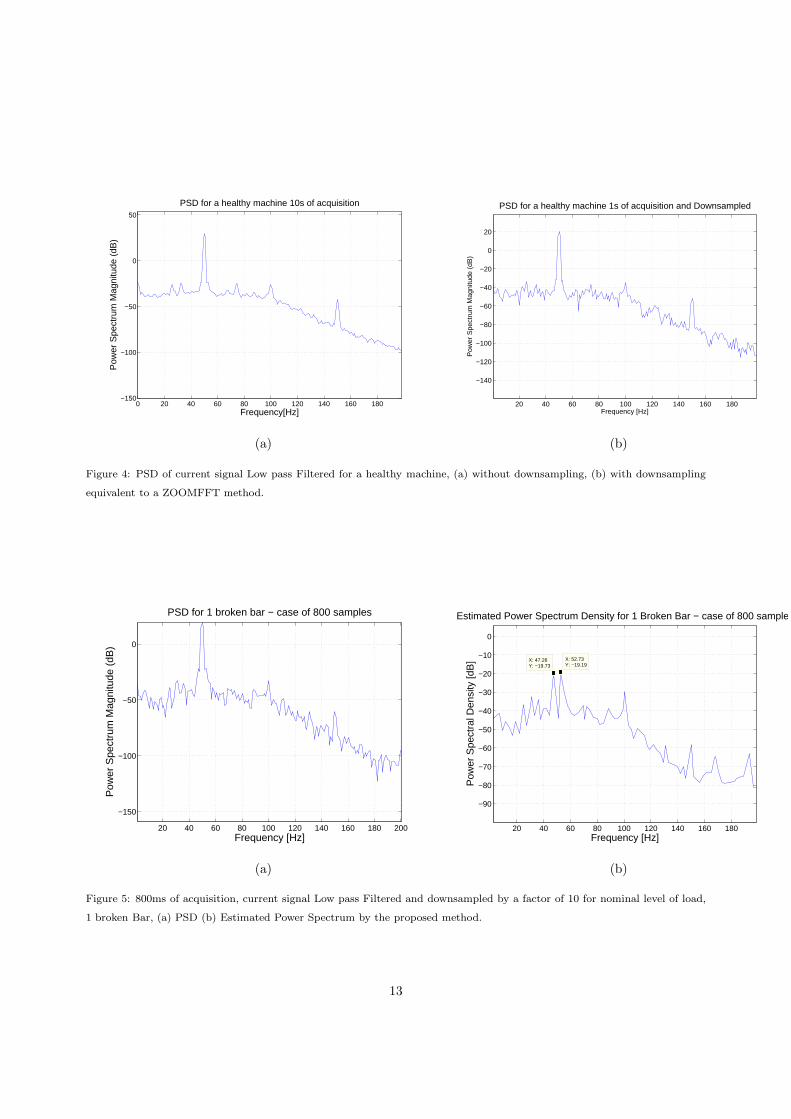
We then wanted to have an idea whether a refined FFT-algorithm, such as the ZOOMFFT technique (see

the references of [7]) could improve the estimation of the sidebands. The principle is to low-pass filter the

10s of the healthy machine at nominal level of load with a cut of frequency of 100 Hz (Fig.3-(a)) and next

downsample it by a factor of 10. We observe that once again, this procedure is unable to estimate the

sidebands components around the driven frequency, Fig.4 draws that fact.

In short, we have shown that for 10s of acquisition, low-pass filtered and downsampled by a factor of 10,

leading to a new sampling frequency equal to 1 KHz; the proposed method which integrates the 50 Hz and

for which an oblique pre-processing followed by a TLS solution is employed was clearly better than classical

PSD or FFT-based analysis for spectrum estimation. This fundamental observation, developed for the case

of a healthy machine at nominal level of load is furthermore reinforced by the results depicted in Fig.5

and Fig.6 for which the machine has 1 broken bar at respectively nominal and low level of load. Finally,

with no ambiguity, whatever the load and the number of broken bars, Fig.5 to Fig.8, the proposed method

undisputedly gives the frequencies related to the sidebands. This estimation will next help us when it comes

to using a diagnosis indicator.

5.3. A diagnosis though improved

In this part, we exploit the frequencies related to the sidebands components for they help to have an

indicator of the rotor bars state. We use so the concept of power ratio between the supply frequency and

the sidebands components [25], with for example [27]

I =∑

k∈S

(s2ks20

)

where S = {k ∈ Z∗ | fsb = (1 + 2kg)fr is estimated}. We have used this indicator in conjunction with the

high resolution method proposed in [27] for the same conditions as for the experience of Fig.3-(b), 5 and 7.

The results are reported inside table1.

11

20 40 60 80 100 120 140 160 180

−60

−40

−20

0

20

40

Frequency [Hz]

Pow

er S

pect

rum

Mag

nitu

de (

dB)

PSD for a healthy machine 10s of acquisition

0.02 0.04 0.06 0.08 0.1 0.12 0.14 0.16 0.18

−110

−100

−90

−80

−70

−60

−50

−40

−30

−20

−10

Frequency (kHz)

Pow

er/fr

eque

ncy

(dB

/Hz)

Welch Power Spectral Density Estimate

(a) (b)

Figure 2: 10s of acquisition for a healthy machine, (a) PSD, (b) Welch Estimator with optimal overlapping windows

0 500 1000 1500 2000 2500 3000 3500 4000 4500 5000−1000

−800

−600

−400

−200

0

Frequency (Hz)

Ph

ase

(d

eg

ree

s)

0 500 1000 1500 2000 2500 3000 3500 4000 4500 5000−800

−600

−400

−200

0

Frequency (Hz)

Ma

gn

itu

de

(d

B)

Frequency response of the Low pass Filter

20 40 60 80 100 120 140 160 180 200

−90

−80

−70

−60

−50

−40

−30

−20

−10

0

X: 52.49Y: −30.39

X: 47.57Y: −29.01

Frequency [Hz]

Pow

er S

pect

ral D

ensi

ty [d

B]

Estimated Power spectrum for a healthy machine 1s of acquisition

(a) (b)

Figure 3: (a) Low-pass frequency response, cut off frequency 100 Hz, (b) 1s of acquisition, current signal Low pass Filtered

and downsampled by a factor of 10 for nominal level of load, healthy machine, Estimated Power Spectrum by the proposed

method.

State fr (Hz) k 2gfr (Hz) I (×10−4)

Healthy 49.98 ±1 0.6 3.12

1 Broken Bar 50.31 ±1 1.2 796

2 Broken Bars 49.82 ±{1, 2, 3} 1.4 4147

Table 1:

12

0 20 40 60 80 100 120 140 160 180−150

−100

−50

0

50

Frequency[Hz]

Pow

er S

pect

rum

Mag

nitu

de (

dB)

PSD for a healthy machine 10s of acquisition

20 40 60 80 100 120 140 160 180

−140

−120

−100

−80

−60

−40

−20

0

20

Frequency [Hz]

Pow

er S

pect

rum

Mag

nitu

de (

dB)

PSD for a healthy machine 1s of acquisition and Downsampled

(a) (b)

Figure 4: PSD of current signal Low pass Filtered for a healthy machine, (a) without downsampling, (b) with downsampling

equivalent to a ZOOMFFT method.

20 40 60 80 100 120 140 160 180 200

−150

−100

−50

0

Frequency [Hz]

Pow

er S

pect

rum

Mag

nitu

de (

dB)

PSD for 1 broken bar − case of 800 samples

20 40 60 80 100 120 140 160 180

−90

−80

−70

−60

−50

−40

−30

−20

−10

0

X: 52.73Y: −19.19

X: 47.26Y: −19.73

Frequency [Hz]

Pow

er S

pect

ral D

ensi

ty [d

B]

Estimated Power Spectrum Density for 1 Broken Bar − case of 800 samples

(a) (b)

Figure 5: 800ms of acquisition, current signal Low pass Filtered and downsampled by a factor of 10 for nominal level of load,

1 broken Bar, (a) PSD (b) Estimated Power Spectrum by the proposed method.

13

20 40 60 80 100 120 140 160 180 200

−140

−120

−100

−80

−60

−40

−20

0

20

Frequency [Hz]

Pow

er S

pect

rum

Mag

nitu

de (

dB)

PSD for 1 broken bar − case of 800 samples

20 40 60 80 100 120 140 160 180

−90

−80

−70

−60

−50

−40

−30

−20

−10

0

X: 52.68Y: −19.47

X: 47.3Y: −19.67

Frequency [Hz]

Pow

er S

pect

ral D

ensi

ty [d

B]

Estimated Power Spectrum for 1 broken Bar − case of 800 samples

(a) (b)

Figure 6: 800ms of acquisition, current signal Low pass Filtered and downsampled by a factor of 10 for low level of load, 1

broken Bar, (a) PSD (b) Estimated Power Spectrum by the proposed method.

20 40 60 80 100 120 140 160 180

−150

−100

−50

0

X: 57Y: −31.91

X: 43Y: −32.49

Frequency [Hz]

Pow

er S

pect

rum

Mag

nitu

de (

dB)

PSD of 2 broken bars − case 1000 samples

20 40 60 80 100 120 140 160 180 200

−90

−80

−70

−60

−50

−40

−30

−20

−10

0X: 52.51Y: −11.8

Frequency [Hz]

X: 47.52Y: −12.86

X: 42.56Y: −30.23

X: 57.5Y: −28.8

Pow

er S

pect

ral D

ensi

ty [d

B]

Estimated Power Spectrum Density for 2 Broken Bars − case of 1000 samples

(a) (b)

Figure 7: 1s of acquisition, current signal Low pass Filtered and downsampled by a factor of 10 for nominal level of load, 2

broken Bars, (a) PSD (b) Estimated Power Spectrum by the proposed method.

14

0 20 40 60 80 100 120 140 160 180 200

−150

−100

−50

0

X: 57Y: −32.1

X: 43Y: −31.78

Frequency [Hz]

Pow

er S

pect

rum

Mag

nitu

de (

dB)

PSD for 2 Broken Bars

20 40 60 80 100 120 140 160 180 200−100

−90

−80

−70

−60

−50

−40

−30

−20

−10

0

X: 57.5Y: −28.79

Frequency [Hz]

Pow

er S

pect

ral D

ensi

ty [d

B]

X: 52.5Y: −11.79

X: 47.52Y: −12.87

X: 42.56Y: −30.24

Estimated Power Spectrum for 2 Broken Bars − case of 1000 samples (1s of acquisition)

(a) (b)

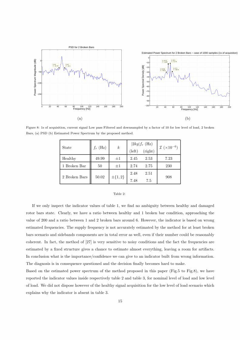
Figure 8: 1s of acquisition, current signal Low pass Filtered and downsampled by a factor of 10 for low level of load, 2 broken

Bars, (a) PSD (b) Estimated Power Spectrum by the proposed method.

State fr (Hz) k|2kg|fr (Hz)

I (×10−6)(left) (right)

Healthy 49.99 ±1 2.45 2.53 7.23

1 Broken Bar 50 ±1 2.74 2.75 230

2 Broken Bars 50.02 ±{1, 2}2.48 2.51

9087.48 7.5

Table 2:

If we only inspect the indicator values of table 1, we find no ambiguity between healthy and damaged

rotor bars state. Clearly, we have a ratio between healthy and 1 broken bar condition, approaching the

value of 200 and a ratio between 1 and 2 broken bars around 6. However, the indicator is based on wrong

estimated frequencies. The supply frequency is not accurately estimated by the method for at least broken

bars scenario and sidebands components are in total error as well, even if their number could be reasonably

coherent. In fact, the method of [27] is very sensitive to noisy conditions and the fact the frequencies are

estimated by a fixed structure gives a chance to estimate almost everything, leaving a room for artifacts.

In conclusion what is the importance/confidence we can give to an indicator built from wrong information.

The diagnosis is in consequence questioned and the decision finally becomes hard to make.

Based on the estimated power spectrum of the method proposed in this paper (Fig.5 to Fig.8), we have

reported the indicator values inside respectively table 2 and table 3, for nominal level of load and low level

of load. We did not dispose however of the healthy signal acquisition for the low level of load scenario which

explains why the indicator is absent in table 3.

15

State fr (Hz) k|2kg|fr (Hz)

I (×10−6)(left) (right)

1 Broken Bar 50 ±1 2.68 2.7 245

2 Broken Bars 50.01 ±{1, 2}2.48 2.5

15007.44 7.5

Table 3:

Whatever the load conditions, thanks to a better estimated power spectrum, the sidebands components

are better estimated and the diagnosis indicator is more significant . From the results of tables 2 and table

3, we easily see the difference between healthy and failure conditions. The ratio between a healthy and

damaged condition is around 30, which leaves no doubt about the decision to make. Similarly, the difference

between 1 and 2 broken bars is significant. We have first the number of harmonics growing from 1 to 2

with odd harmonics accurately estimated and next inevitably the increase of the indicator value. The ratio

between 1 and 2 broken bars of the latter is for example in between 4 and 7 with the highest difference for

the low level of load.

6. Conclusion

One of the ways to come to a reliable diagnosis on a machine from current acquisition is to inspect

an indicator based on the ratio between the supply frequency and its sidebands components. For different

actual operations, the load strongly impacts on the proximity of the sidebands to the driven frequency. The

challenge is therefore to be able to estimate these sidebands and especially for low level of load. Classical

approaches based on periodogram or FFT-based analysis have shown their inadequacy for such a difficult

problem. The idea developed in this paper is then to overcome this difficulty by using a high resolution

method designed with the support of the supply frequency. The purpose is therefore to suppress this partic-

ular and harmful frequency in the set of frequencies of interest. This method has already been introduced

and it gives accurate frequency estimation with a sufficient resolution, allowing to precisely discriminate

frequencies such as sidebands. The major point is that the driven frequency no longer exists. The next

treatment consists in estimating the power associated with the remaining frequencies. In this paper, we

propose to first pre-process the data observation by obliquely projecting it onto a subspace which would be

associated with the spectrum of interest, i.e. without the supply frequency, along the subspace in which the

supply frequency would live. This consequently accounts for the supply frequency in the data observation

and then cancels (almost) its influence on the power spectrum. Once this pre-processing of the data ob-

servation has been done, we propose a Total Least Squares (TLS) estimation procedure to finally have the

power of each frequency without the impact of the very powerful supply frequency. We have tested this pro-

16

cedure in different conditions of load, nominal or low level, for healthy, 1 broken and 2 broken bars against

classical FFT analysis, ZOOMFFT method and MUSIC-like criterion especially designed for mechanical de-

fects diagnosing. The results observed for short acquisition duration have clearly shown the limits of these

methods. Conversely, the diagnosis given by an indicator based on the power spectrum estimated by the

present approach is sure and robust to the load conditions and number of broken bars; even for challenging

scenarios.

References

[1] M. Benbouzid, A Review of Induction Motors Signature Analysis as a Medium for Faults Detection, IEEE Trans. on

Industrial electronics 47 (5) (2000) 984–994.

[2] J. Jung, J. Lee, B. Kwon, Online diagnosis of induction motors using MCSA, IEEE Trans. on Industrial Electronics 53 (6)

(2006) 1842–1852.

[3] A. Menacer, S. Moreau, G. Champenois, M. Said, A. Benakcha, Experimental Detextion of Rotor Failures of Induc-

tion Machines by Stator Current Spectrum Analysis in Function of the Broken rotor Bars Position and the Load, The

International Conference on Computer as a Tool (2007) 1752–1758.

[4] Z. Peng, F. Chu, Application of the wavelet transform in machine condition monitoring and fault diagnostics: a review

with bibliography, Mechanical Systems and Signal Processing 18 (2) (2004) 199 – 221.

[5] A. K. S. Jardine, D. Lin, D. Banjevic, A review on machinery diagnostics and prognostics implementing condition-based

maintenance, Mechanical Systems and Signal Processing 20 (7) (2006) 1483 – 1510.

[6] P. Jayaswal, A. K. Wadhwani, K. B. Mulchandani, Review Article Machine Fault Signature Analysis, International Journal

of Rotating Machinery.

[7] M. Mehrjou, N. Mariun, M. Marhaban, N. Misron, Rotor fault condition monitoring techniques for squirrel-cage induction

machine—a review, Mechanical Systems and Signal Processing 25 (8) (2011) 2827 – 2848.

[8] L. A. Garcıa-Escudero, O. Duque-Perez, D. Morinigo-Sotelo, M. Perez-Alonso, Robust condition monitoring for early

detection of broken rotor bars in induction motors, Expert Systems with Applications 38 (3) (2011) 2653 – 2660.

[9] V. T. Tran, B.-S. Yang, An intelligent condition-based maintenance platform for rotating machinery, Expert Systems with

Applications 39 (3) (2012) 2977–2988.

[10] G. Didier, E. Ternisien, O. Caspary, H. Razik, A new approach to detect broken rotor bars in induction machines by

current spectrum analysis, Mechanical Systems and Signal Processing 21 (2) (2007) 1127 – 1142.

[11] P. Zhang, S. Ding, G. Wang, D. Zhou, A frequency domain approach to fault detection in sampled-data systems, Auto-

matica 39 (7) (2003) 1303 – 1307.

[12] G. Dalpiaz, A. Rivola, Condition monitoring and diagnostics in automatic machines: Comparison of vibration analysis

techniques, Mechanical Systems and Signal Processing 11 (1) (1997) 53 – 73.

[13] H. R. A. Abed, L. Baghli, A. Rezzoug, Modelling Induction Motors for Diagnostic Purposes, European Conference on

power Electronics and Applications (1999) 1–8.

[14] R. Casimir, E. Bouteleux, H. Yahoui, G. Clerc, H. Henao, C. Delmotte, G.-A. Capolino, G. Rostaing, J.-P. Rognon,

E. Foulon, L. Loron, H. Razik, G. Didier, G. Houdouin, G. Barakat, B. Dakyo, S. Bachir, S. Tnani, G. Champenois, J.-C.

Trigeassou, V. Devanneaux, B. Dagues, J. Faucher, Comparison of modelling methods and of diagnostic of asynchronous

motor in case of defects, in: 9th IEEE International Power Electronics Congress, 2004, pp. 101 – 108.

[15] C. Cristalli, N. Paone, R. Rodrıguez, Mechanical fault detection of electric motors by laser vibrometer and accelerometer

measurements, Mechanical Systems and Signal Processing 20 (6) (2006) 1350 – 1361.

17

[16] A. Siddique, G. Yadava, B. Singh, A review of stator fault monitoring techniques of induction motors, IEEE Transactions

on Energy Conversion 20 (1) (2005) 106 – 114.

[17] K. Worden, W. J. Staszewski, J. J. Hensman, Natural computing for mechanical systems research: A tutorial overview,

Mechanical Systems and Signal Processing 25 (1) (2011) 4–111.

[18] A. Widodo, B.-S. Yang, Support vector machine in machine condition monitoring and fault diagnosis, Mechanical Systems

and Signal Processing 21 (6) (2007) 2560 – 2574.

[19] Y.Lei, J. Lin, Z. He, M. J. Zuo, A review on empirical mode decomposition in fault diagnosis of rotating machinery,

Mechanical Systems and Signal Processing 35 (1–2) (2013) 108 – 126.

[20] N. Hamzaoui, C. Boisson, C. Lesueur, Vibro–acoustic analysis and identification of defects in rotating machinery, part i:

Theoretical model, Journal of Sound and Vibration 216 (4) (1998) 553 – 570.

[21] R. Randall, Vibration-based Condition Monitoring: Industrial, Aerospace and Automotive Applications, Wiley online

library, Wiley, 2011.

[22] G. Didier, E. Ternisien, O. Caspary, H. Razik, Fault detection of broken rotor bars in induction motor using a global fault

index, IEEE Transactions on Industry Applications 42 (1) (2006) 79–88.

[23] M. Eltabach, J. Antoni, G. Shanina, S. Sieg-Zieba, X. Carniel, Broken rotor bars detection by a new non-invasive diagnostic

procedure, Mechanical Systems and Signal Processing 23 (2009) 1398 – 1412.

[24] M. Eltabach, J. Antoni, M. Najjar, Quantitative analysis of noninvasive diagnostic procedures for induction motor drives,

Mechanical Systems and Signal Processing 21 (7) (2007) 2838 – 2856.

[25] A. Bellini, F. Filippetti, C. Tassoni, G.-A. Capolino, Advances in Diagnostic Techniques for Induction Machines, IEEE

Transactions on Industrial Electronics 55 (12) (2008) 4109–4126.

[26] A. da Silva, Induction motor fault diagnostic and monitoring methods, Ph.D. thesis, Marquette University, Milwaukee,

Wisconsin (May 2006).

[27] E. ElBouchikhi, V. Choqueuse, M. Benbouzid, J. Charpentier, Induction machine fault detection enhancement using a

stator current high resolution spectrum, in: 38th Annual Conference on IEEE Industrial Electronics Society (IECON),

2012, pp. 3913–3918.

[28] G. King, M. Tarbouchi, D. McGaughey, Current signature analysis of induction machine rotor faults using the fast

orthogonal search algorithm, in: 5th IET International Conference on Power Electronics, Machines and Drives (PEMD

2010), IEE, 2010, p. 215.

[29] D. R. McGaughey, M. Tarbouchi, K. Nutt, A. Chikhani, Speed sensorless estimation of ac induction motors using the fast

orthogonal search algorithm, IEEE Transactions on Energy Conversion 21 (1) (2006) 112–120.

[30] K. H. Chon, Accurate identification of periodic oscillations buried in white or colored noise using fast orthogonal search,

IEEE Transactions on Biomedical Engineering 48 (6) (2001) 622–629.

[31] A. Bracale, G. Carpinelli, L. Piegari, P. Tricoli, A High Resolution Method for On Line Diagnosis of Induction Motors

Faults, IEEE Power Tech 2007 (2007) 994–998.

[32] S. Kia, H. Henao, G.-A. Capolino, A High-resolution frequency estimation method for three-phase induction machine fault

detection, IEEE Trans. on Industrial Electronics 54 (4) (2007) 2305–2314.

[33] G. Bouleux, A. Ibrahim, F. Guillet, R. Boyer, A subspace-based rejection method for detecting bearing fault in asyn-

chronous motor, in: International Conference on Condition Monitoring and Diagnosis (CMD), 2008, pp. 171–174.

[34] G. Bouleux, T. Kidar, F. Guillet, An improper random vector approach for esprit and unitary esprit frequency estimation,

in: 7th International Workshop on Systems Signal Processing and their Applications (WOSSPA), 2011, pp. 299–302.

[35] P. Wirfalt, G. Bouleux, M. Jansson, P. Stoica, Subspace-based frequency estimation utilizing prior information, in: IEEE

Statistical Signal Processing Workshop (SSP), 2011, pp. 533–536.

[36] M. Kristensson, M. Jansson, B. Ottersten, Further results and insights on subspace based sinusoidal frequency estimation,

18

IEEE Trans. on Signal Processing 49 (12) (2001) 2962–2974.

[37] G. Bouleux, P. Stoica, R. Boyer, An Optimal Prior knowledge-based DOA Estimation Method, in: 17th European Signal

Processing Conference, 2009.

[38] H. Chen, S. V. Huffel, D. V. Ormondt, R. de Beer, Parameter Estimation with Prior Knowledge of Known Signal Poles

for the Quantification of NMR Spectroscopy Data in the Time Domain, Journal of Magnetic Resonance 119 (2) (1996)

225–234.

[39] R. Behrens, L. Scharf, Signal Processing Applications of Oblique Projection Operators, IEEE Trans. on Signal Processing

42 (6) (1994) 1413–1424.

[40] S. V. Huffel, J. Vanderwalle, The total least squares problem : computational aspects and analysis, SIAM Publications,

1991.

19