Embed Size (px)
Citation preview
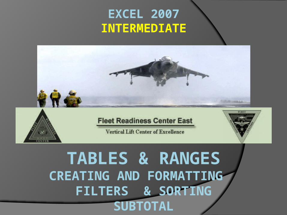
EXCEL 2007INTERMEDIATE
TABLES & RANGESCREATING AND FORMATTING
FILTERS & SORTINGSUBTOTAL
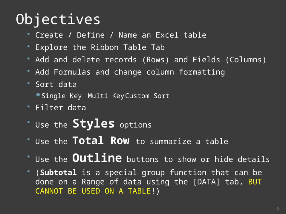
Objectives Create / Define / Name an Excel table Explore the Ribbon Table Tab Add and delete records (Rows) and Fields (Columns) Add Formulas and change column formatting Sort data
Single Key Multi Key Custom Sort
Filter data
Use the Styles options
Use the Total Row to summarize a table
Use the Outline buttons to show or hide details
(Subtotal is a special group function that can be done on a Range of data using the [DATA] tab, BUT CANNOT BE USED ON A TABLE!) 2
Structured Range of Data
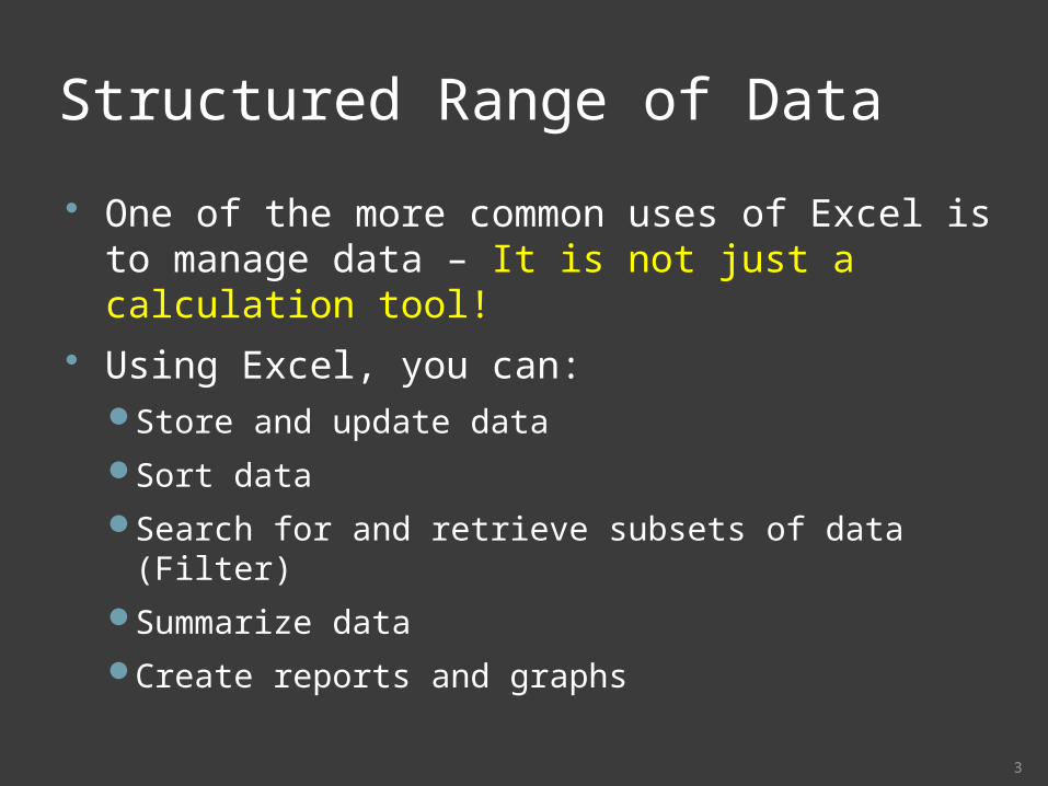
One of the more common uses of Excel is to manage data – It is not just a calculation tool!
Using Excel, you can:Store and update data
Sort data
Search for and retrieve subsets of data (Filter)
Summarize data
Create reports and graphs
3
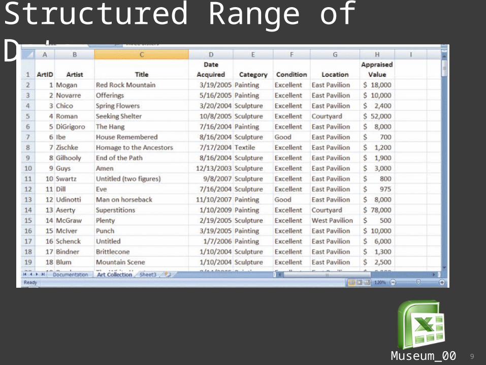
Structured Range of Data
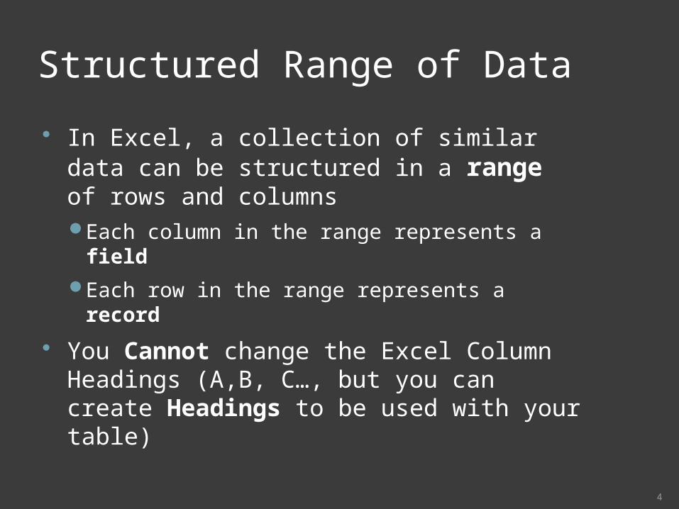
In Excel, a collection of similar data can be structured in a range of rows and columnsEach column in the range represents a field
Each row in the range represents a record
You Cannot change the Excel Column Headings (A,B, C…, but you can create Headings to be used with your table)
4
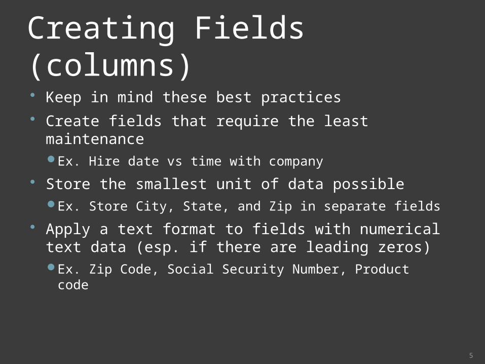
Creating Fields (columns) Keep in mind these best practices Create fields that require the least maintenance
Ex. Hire date vs time with company
Store the smallest unit of data possibleEx. Store City, State, and Zip in separate fields
Apply a text format to fields with numerical text data (esp. if there are leading zeros)Ex. Zip Code, Social Security Number, Product code
5
Structured References
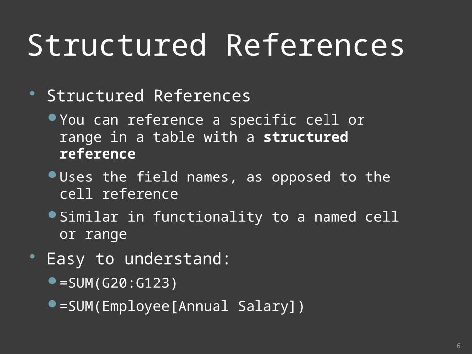
Structured ReferencesYou can reference a specific cell or range in a
table with a structured reference
Uses the field names, as opposed to the cell reference
Similar in functionality to a named cell or range
Easy to understand:=SUM(G20:G123)
=SUM(Employee[Annual Salary])
6
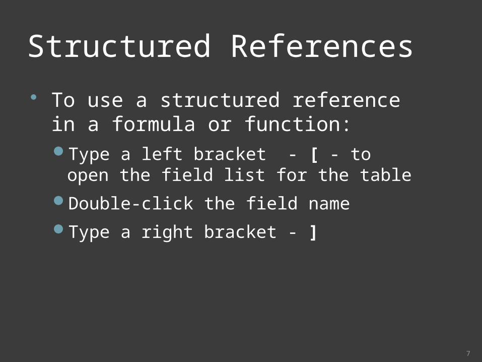
Structured References
To use a structured reference in a formula or function:Type a left bracket - [ - to open the field list
for the table
Double-click the field name
Type a right bracket - ]
7
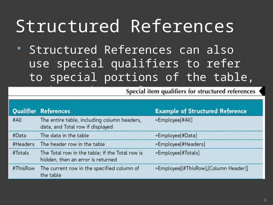
Structured References Structured References can also use special
qualifiers to refer to special portions of the table, such as the Total Row.
8
Structured Range of Data
9Museum_00
Tables Range of related data, managed separate
from other data on a worksheet
Easy access to data management and analysis tools
Can have multiple tables in a worksheet
10
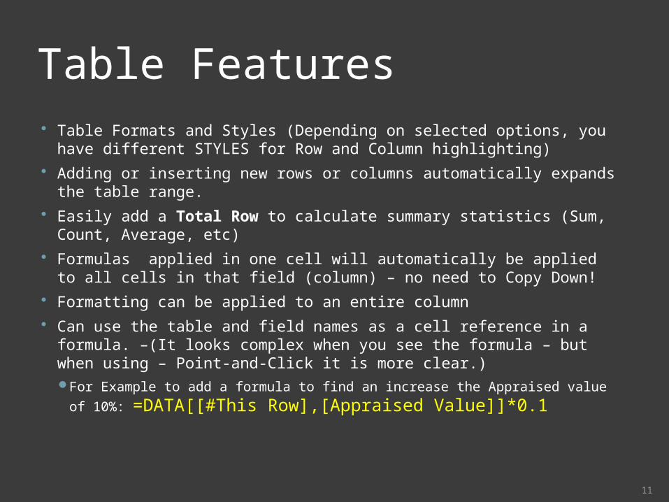
Table Features Table Formats and Styles (Depending on selected options, you have
different STYLES for Row and Column highlighting) Adding or inserting new rows or columns automatically expands the
table range. Easily add a Total Row to calculate summary statistics (Sum,
Count, Average, etc) Formulas applied in one cell will automatically be applied to all cells
in that field (column) – no need to Copy Down! Formatting can be applied to an entire column Can use the table and field names as a cell reference in a formula. –
(It looks complex when you see the formula – but when using – Point-and-Click it is more clear.) For Example to add a formula to find an increase the Appraised value of
10%: =DATA[[#This Row],[Appraised Value]]*0.1
11
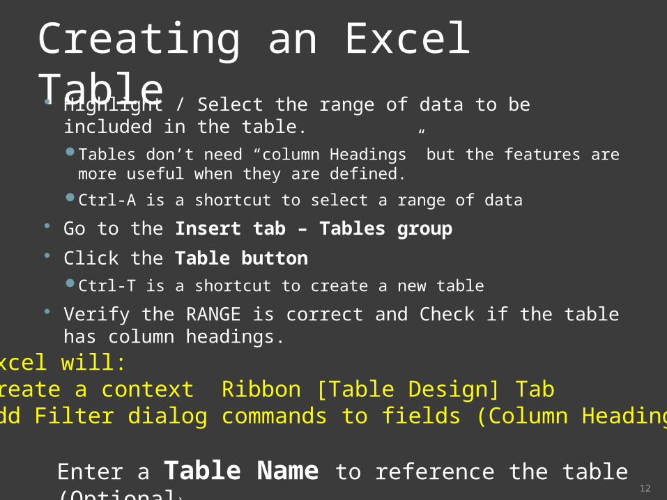
Creating an Excel Table Highlight / Select the range of data to be included in the table.
Tables don’t need “column Headings” but the features are more useful when they are defined.
Ctrl-A is a shortcut to select a range of data
Go to the Insert tab – Tables group Click the Table button
Ctrl-T is a shortcut to create a new table
Verify the RANGE is correct and Check if the table has column headings.
12
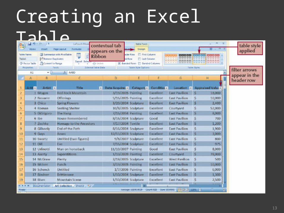
Excel will:Create a context Ribbon [Table Design] Tab Add Filter dialog commands to fields (Column Headings)
Enter a Table Name to reference the table (Optional)
Creating an Excel Table
13
14
Using a Structured Table
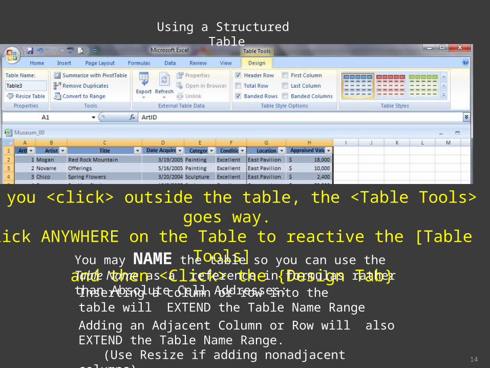
If you <click> outside the table, the <Table Tools> goes way.Click ANYWHERE on the Table to reactive the [Table Tools]
and then <Click> the {Design Tab}You may NAME the table so you can use the Table Name as a reference in formulas rather than Absolute Cell Addresses:
Inserting a column or row into the table will EXTEND the Table Name Range
Adding an Adjacent Column or Row will also EXTEND the Table Name Range.
(Use Resize if adding nonadjacent columns)
15
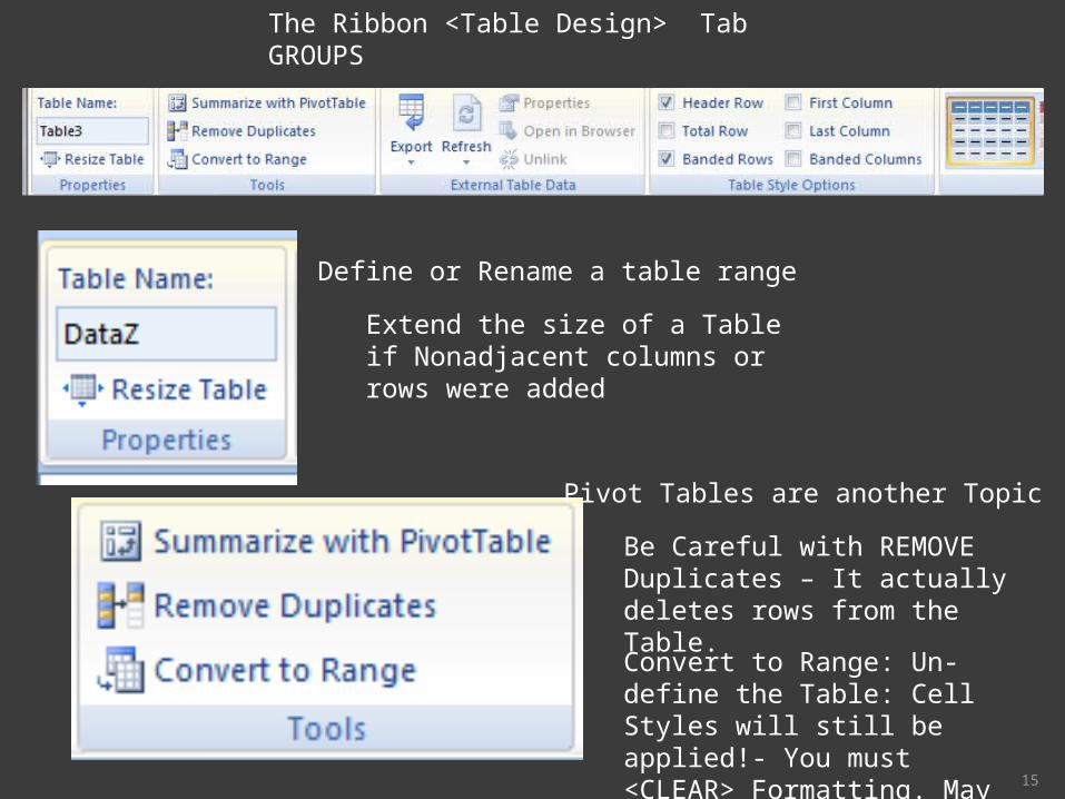
The Ribbon <Table Design> Tab GROUPS
Define or Rename a table range
Extend the size of a Table if Nonadjacent columns or rows were added
Pivot Tables are another Topic
Be Careful with REMOVE Duplicates – It actually deletes rows from the Table.
Convert to Range: Un-define the Table: Cell Styles will still be applied!- You must <CLEAR> Formatting. May also cause problems with Defined Formulas
16
The Ribbon <Table Design> Tab GROUPS
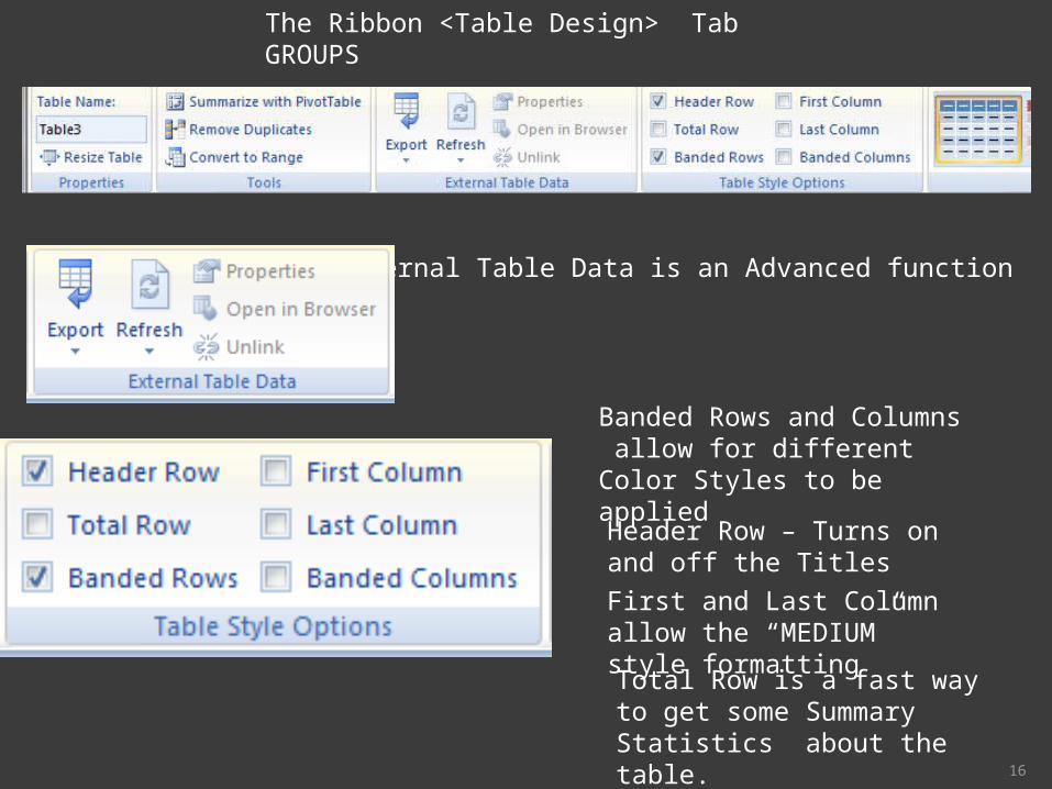
External Table Data is an Advanced function
Banded Rows and Columns allow for different Color Styles to be applied
Header Row – Turns on and off the Titles
First and Last Column allow the “MEDIUM” style formatting
Total Row is a fast way to get some Summary Statistics about the table.
Using the Total Row
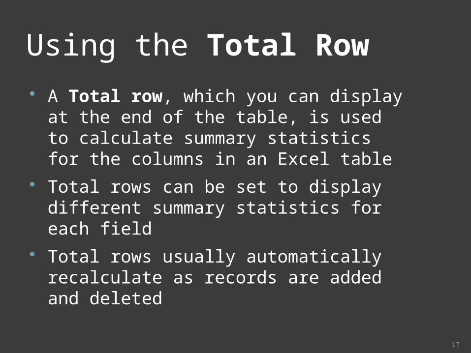
A Total row, which you can display at the end of the table, is used to calculate summary statistics for the columns in an Excel table
Total rows can be set to display different summary statistics for each field
Total rows usually automatically recalculate as records are added and deleted
17
Using the Total Row
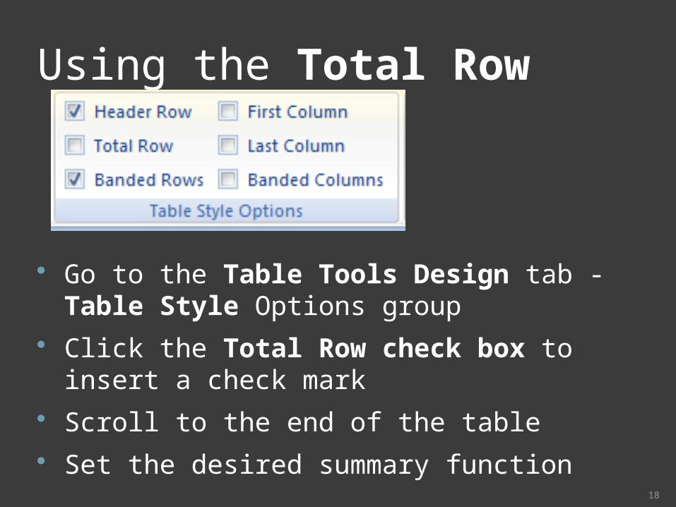
Go to the Table Tools Design tab - Table Style Options group
Click the Total Row check box to insert a check mark
Scroll to the end of the table Set the desired summary function
18
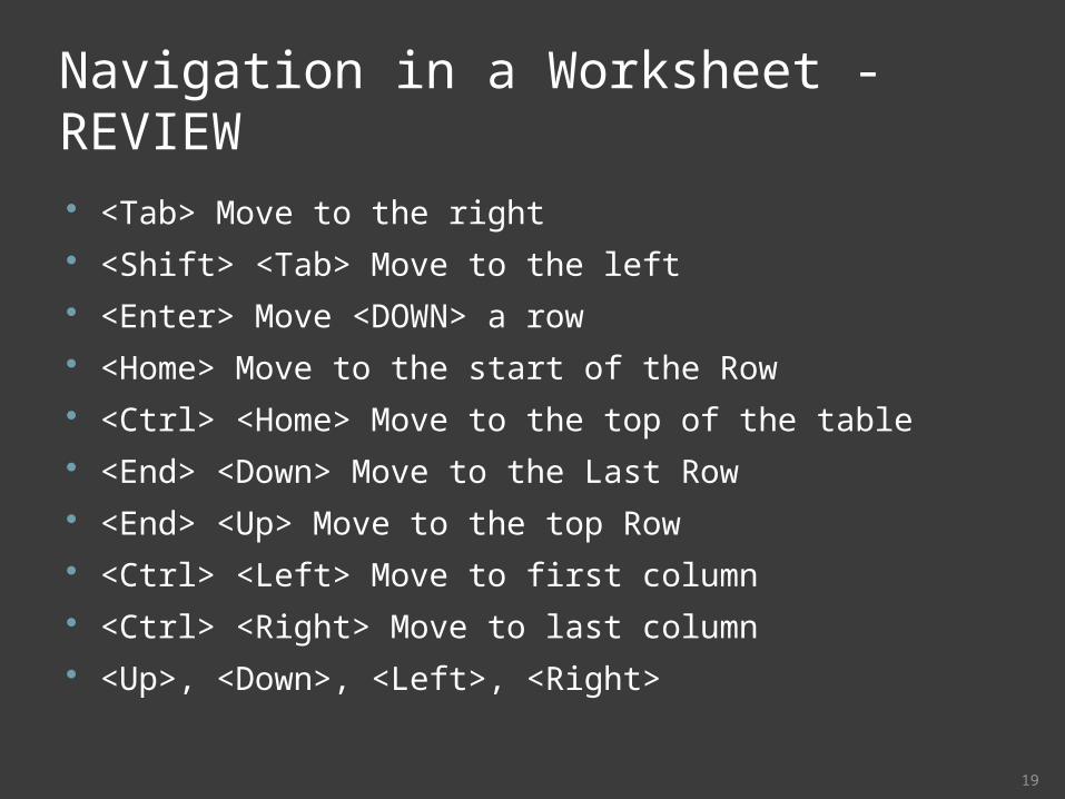
Navigation in a Worksheet - REVIEW <Tab> Move to the right <Shift> <Tab> Move to the left <Enter> Move <DOWN> a row <Home> Move to the start of the Row <Ctrl> <Home> Move to the top of the table <End> <Down> Move to the Last Row <End> <Up> Move to the top Row <Ctrl> <Left> Move to first column <Ctrl> <Right> Move to last column <Up>, <Down>, <Left>, <Right>
19
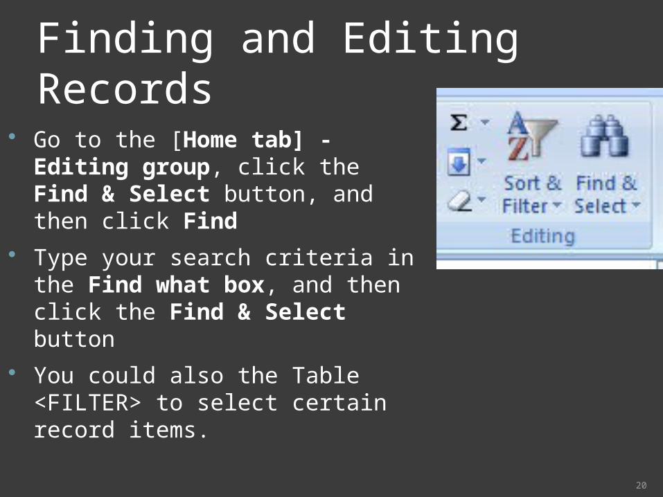
Finding and Editing Records
Go to the [Home tab] - Editing group, click the Find & Select button, and then click Find
Type your search criteria in the Find what box, and then click the Find & Select button
You could also the Table <FILTER> to select certain record items.
20
Exercise – Table #1 – Table Creation
Create a table Renaming a table Formatting a table
STYLES
Column Formats
Adding a Column Adding and Deleting records Adding the TOTAL ROW
21

22
SORTING AND
FILTERING
Sorting and Filtering Allows data to be viewed differently from how it was
entered
Key functionality of Excel when used to manage data
Sort rearranges the data in a table or range, based on the sort criteria(Any SUBTOTALS applied will be reset with a SORT
Filters present the data that meets the filter criteria.
Filters can be applied to multiple columns
When using Filters, care must be taken that you are reporting the data you really want to show!
23
Sorting Data You can rearrange, or sort, the records in a
table or range based on the data in one or more fields (Old Limit was 3 levels of sorting)
The fields you use to order the data are called sort fields
You can sort data in ascending (A-Z) or descending (Z-A) order, unless using a custom list
24
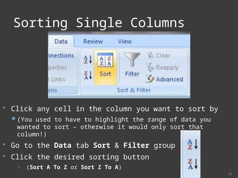
Sorting Single Columns
Click any cell in the column you want to sort by(You used to have to highlight the range of data you wanted to
sort – otherwise it would only sort that column!)
Go to the Data tab Sort & Filter group
Click the desired sorting button○ (Sort A To Z or Sort Z To A)
25
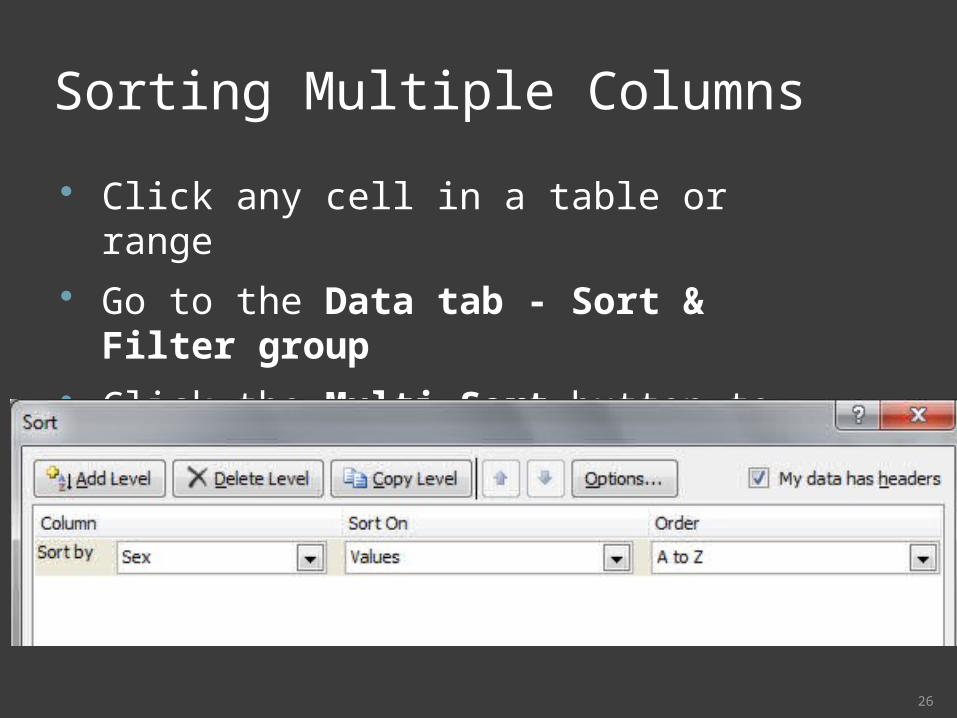
Sorting Multiple Columns Click any cell in a table or range
Go to the Data tab - Sort & Filter group
Click the Multi Sort button to open the Sort dialog box
26
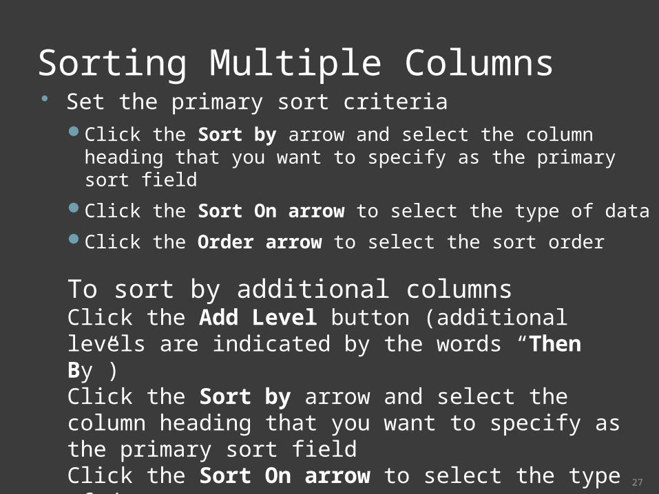
Sorting Multiple Columns Set the primary sort criteria
Click the Sort by arrow and select the column heading that you want to specify as the primary sort field
Click the Sort On arrow to select the type of data
Click the Order arrow to select the sort order
27
To sort by additional columnsClick the Add Level button (additional levels are indicated by the words “Then By”)Click the Sort by arrow and select the column heading that you want to specify as the primary sort fieldClick the Sort On arrow to select the type of dataClick the Order arrow to select the sort order
Sorting Using a Custom List A custom list allows you to indicate the sequence
in which you want data ordered
Used when you want to sort text data outside of the normal Ascending and Descending methods
Can use predefined custom lists or define your own.
IE:Months: Jan, Feb, Mar, April, May, June….
Days: Sun, Mon, Tues, Wed, …
Region: North, West, South, East, South West
Condition: Poor, Fair, Good, Excellent28
Sorting Using a Custom List Go to the Data tab - Sort & Filter group
Click the Sort button
Click the Order arrow, and then click Custom List
In the List entries box, type each entry for the custom list, pressing the Enter key after each entry
Click the Add button
Click the OK button
29
Exercise # 2 – Sorting
Sorting by One Column Sorting Data using Multiple Columns Sorting using a custom list
30
31
FILTERING
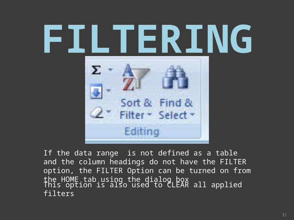
If the data range is not defined as a table and the column headings do not have the FILTER option, the FILTER Option can be turned on from the HOME tab using the dialog box
This option is also used to CLEAR all applied filters
Filtering
Excel automatically creates filters when a TABLE is created
Clicking the filter arrow in a column opens the Filter menu for that field
Data can be filtered by:Cell or font colors
Apply Text or Numeric Filters and conditional logic
Select specific values
32
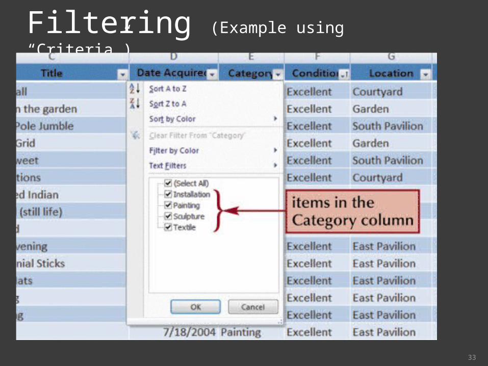
Filtering (Example using “Criteria”)
33
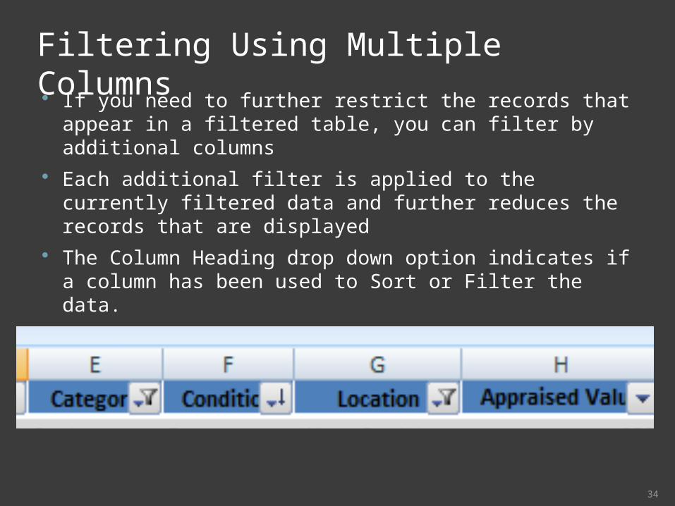
Filtering Using Multiple Columns If you need to further restrict the records that appear
in a filtered table, you can filter by additional columns Each additional filter is applied to the currently filtered
data and further reduces the records that are displayed
The Column Heading drop down option indicates if a column has been used to Sort or Filter the data.
34
35
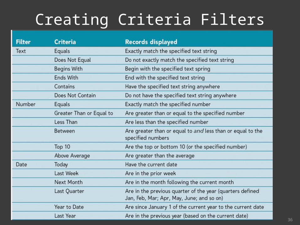
Creating Criteria Filters
Criteria Filters enable you to specify various more complex conditions in addition to those that are based on an “equals” criterion
Different data types have different criteria that can be used in a filter
Criteria Filters and Selection Filters are mutually exclusive. You cannot mix them!
Creating Criteria Filters
36
Creating Criteria Filters
Click on the filter arrow of the field (column) you want to filter by
Select the filter type (usually right above the unique values list). The data type of the field will determine the type of filter available
Select the filter operator If necessary, provide criteria values
37
Exercise #3 - Filters
Filtering by One Column Filtering Data using Multiple Columns Clearing Filters Selecting Multiple Filter Items in One
Column Create a NUMBER Criteria Filter Create a TEXT Criteria Filter
38
Using Subtotals
39
Calculating Subtotals Subtotals are used to summarize a range of data in
Excel Subtotals cannot be applied to an Excel table – if the
data being analyzed is in a Table, it must be removed. (Design – Convert to Range)
The data must be sorted so it is grouped as desired BEFORE applying subtotals to do “Control Breaks” in the correct order: IE:
○ City / Sex / Race Location / Criteria / Artist
○ Race / Grade / Sex Artist / Location / Criteria
○ Sex / Grade / Age
40
Calculating Subtotals Sort the data by the column for which you
want a subtotal FIRST
If the data is in an Excel table, go to the Table Tools Design tab - Tools group, and click the Convert to Range button
Go to the Data tab - Outline group, and click the Subtotal button
Click the At each change in arrow, and then click the column that contains the group you want to subtotal
41
42
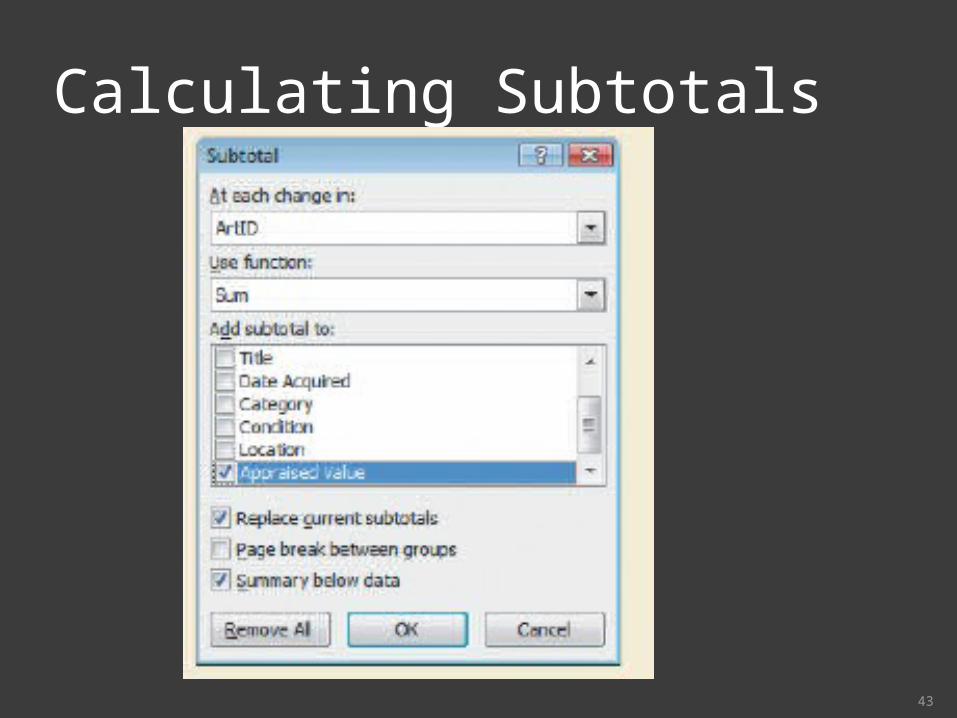
Calculating Subtotals Click the Use function arrow, and then click
the summary function you want to use In the Add subtotal to box, click the check
box for each column that contains the values you want to summarize
To calculate another category of subtotals, click the Replace current subtotals check box to remove the check mark, and then repeat the previous three steps
Click the OK button
Calculating Subtotals
43
Using the Subtotal Outline View
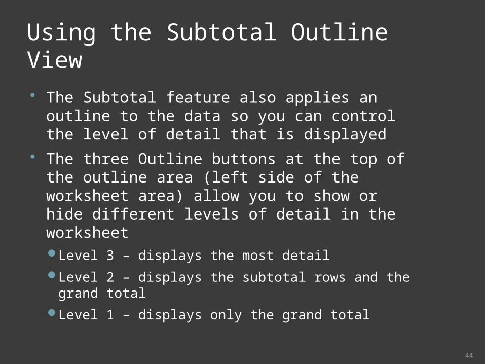
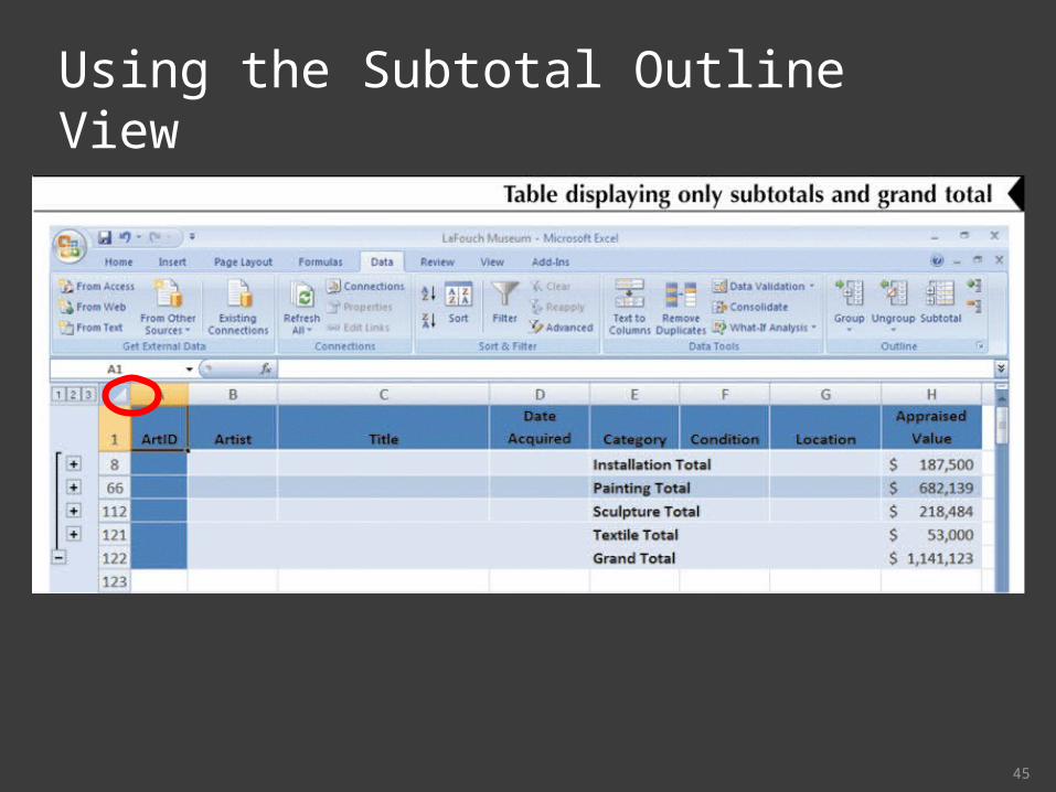
The Subtotal feature also applies an outline to the data so you can control the level of detail that is displayed
The three Outline buttons at the top of the outline area (left side of the worksheet area) allow you to show or hide different levels of detail in the worksheetLevel 3 – displays the most detail
Level 2 – displays the subtotal rows and the grand total
Level 1 – displays only the grand total
44
Using the Subtotal Outline View
45
Using the Subtotal for Student Grades
46
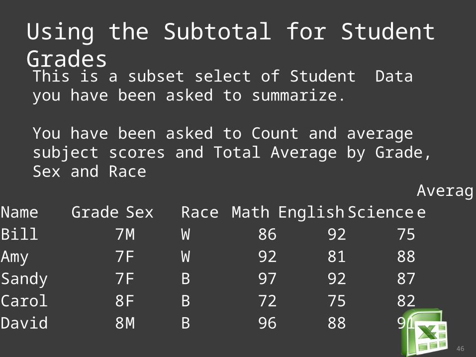
Name Grade Sex Race Math English Science AverageBill 7M W 86 92 75Amy 7F W 92 81 88Sandy 7F B 97 92 87Carol 8F B 72 75 82David 8M B 96 88 91
This is a subset select of Student Data you have been asked to summarize.
You have been asked to Count and average subject scores and Total Average by Grade, Sex and Race
And now for a break…
Can you name these famous Excel cells?The steak sauce cell
The dog cell
The fighter jet cell
The Irish rock group cell
The explosive cell
The vegetable juice cell
47

And now for a break… The steak sauce cell A1 The dog cell K9 The fighter jet cell F16 The Irish rock group cell U2 The explosive cell C4 The vegetable juice cell V8
48