Embed Size (px)
Citation preview

Object and Concept Recognition
for Content-Based Image Retrieval
Yi Li
A dissertation submitted in partial fulfillment ofthe requirements for the degree of
Doctor of Philosophy
University of Washington
2005
Program Authorized to Offer Degree: Computer Science & Engineering


University of WashingtonGraduate School
This is to certify that I have examined this copy of a doctoral dissertation by
Yi Li
and have found that it is complete and satisfactory in all respects,and that any and all revisions required by the final
examining committee have been made.
Chair of the Supervisory Committee:
Linda G. Shapiro
Reading Committee:
Linda G. Shapiro
Jeff A. Bilmes
Marina Meila
Date:


In presenting this dissertation in partial fulfillment of the requirements for the doctoraldegree at the University of Washington, I agree that the Library shall make its copiesfreely available for inspection. I further agree that extensive copying of this dissertation isallowable only for scholarly purposes, consistent with “fair use” as prescribed in the U.S.Copyright Law. Requests for copying or reproduction of this dissertation may be referredto Proquest Information and Learning, 300 North Zeeb Road, Ann Arbor, MI 48106-1346,1-800-521-0600, to whom the author has granted “the right to reproduce and sell (a) copiesof the manuscript in microform and/or (b) printed copies of the manuscript made frommicroform.”
Signature
Date


University of Washington
Abstract
Object and Concept Recognition
for Content-Based Image Retrieval
Yi Li
Chair of the Supervisory Committee:Professor Linda G. Shapiro
Computer Science & Engineering
The problem of recognizing classes of objects in images is important for annotation and
indexing of image and video databases. Users of commercial CBIR systems prefer to pose
their queries in terms of key words. To help automate the indexing process, we represent
images as sets of feature vectors of multiple types of abstract regions, which come from
various segmentation processes. With this representation, we have developed two new al-
gorithms to recognize classes of objects and concepts in outdoor photographic scenes. The
semi-supervised EM-variant algorithm models each abstract region as a mixture of Gaussian
distributions over its feature space. The more powerful generative/discriminative learning
algorithm is a two-phase method. The generative phase normalizes the description length
of images, which can have an arbitrary number of extracted features. In the discrimina-
tive phase, a classifier learns which images, as represented by this fixed-length description,
contain the target object. We have tested our approaches by experimenting with several dif-
ferent data sets and combinations of features. Our results showed a significant improvement
over the published results.


TABLE OF CONTENTS
List of Figures . . . . . . . . . . . . . . . . . . . . . . . . . . . . . . . . . . . . . . . . iii
List of Tables . . . . . . . . . . . . . . . . . . . . . . . . . . . . . . . . . . . . . . . . . v
Chapter 1: Introduction . . . . . . . . . . . . . . . . . . . . . . . . . . . . . . . . . 1
Chapter 2: Related Literature . . . . . . . . . . . . . . . . . . . . . . . . . . . . . 5
Chapter 3: Abstract Region Features . . . . . . . . . . . . . . . . . . . . . . . . . 9
3.1 Color Regions . . . . . . . . . . . . . . . . . . . . . . . . . . . . . . . . . . . . 10
3.2 Texture Regions . . . . . . . . . . . . . . . . . . . . . . . . . . . . . . . . . . 11
3.3 Structure Regions . . . . . . . . . . . . . . . . . . . . . . . . . . . . . . . . . . 11
3.3.1 Color-Consistent Line Clusters . . . . . . . . . . . . . . . . . . . . . . 13
3.3.2 Orientation-Consistent Line Clusters . . . . . . . . . . . . . . . . . . . 13
3.3.3 Spatially-Consistent Line Clusters . . . . . . . . . . . . . . . . . . . . 14
3.4 Other Features . . . . . . . . . . . . . . . . . . . . . . . . . . . . . . . . . . . 16
3.4.1 Blobworld Regions . . . . . . . . . . . . . . . . . . . . . . . . . . . . . 16
3.4.2 Mean Shift Regions . . . . . . . . . . . . . . . . . . . . . . . . . . . . 16
3.4.3 Color Patches and Texture Patches . . . . . . . . . . . . . . . . . . . . 18
3.4.4 Prominent Colors . . . . . . . . . . . . . . . . . . . . . . . . . . . . . . 18
3.5 Summary . . . . . . . . . . . . . . . . . . . . . . . . . . . . . . . . . . . . . . 18
Chapter 4: The EM-variant approach . . . . . . . . . . . . . . . . . . . . . . . . . 22
4.1 Methodology . . . . . . . . . . . . . . . . . . . . . . . . . . . . . . . . . . . . 23
4.1.1 Single-Feature Case . . . . . . . . . . . . . . . . . . . . . . . . . . . . 23
4.1.2 Multiple-Feature Case . . . . . . . . . . . . . . . . . . . . . . . . . . . 25
4.2 EM-Variant Experiments and Results . . . . . . . . . . . . . . . . . . . . . . 26
4.3 EM-variant Extension and Results . . . . . . . . . . . . . . . . . . . . . . . . 28
4.4 Summary . . . . . . . . . . . . . . . . . . . . . . . . . . . . . . . . . . . . . . 37
i

Chapter 5: Generative/Discriminative Approach . . . . . . . . . . . . . . . . . . . 41
5.1 Methodology . . . . . . . . . . . . . . . . . . . . . . . . . . . . . . . . . . . . 41
5.1.1 Single-Feature Case . . . . . . . . . . . . . . . . . . . . . . . . . . . . 41
5.1.2 Multiple-Feature Case . . . . . . . . . . . . . . . . . . . . . . . . . . . 44
5.2 Experiments . . . . . . . . . . . . . . . . . . . . . . . . . . . . . . . . . . . . . 45
5.2.1 Comparison to the EM-Variant Approach of Chapter 4 . . . . . . . . 47
5.2.2 Comparison to the ALIP Algorithm . . . . . . . . . . . . . . . . . . . 47
5.2.3 Comparison to the Machine Translation Approach . . . . . . . . . . . 51
5.2.4 Performance on Groundtruth Data Set . . . . . . . . . . . . . . . . . . 57
5.2.5 Performance of the Structure Feature . . . . . . . . . . . . . . . . . . 58
5.2.6 Performance on Aerial Video Frames . . . . . . . . . . . . . . . . . . . 64
5.3 Summary . . . . . . . . . . . . . . . . . . . . . . . . . . . . . . . . . . . . . . 70
Chapter 6: Localization . . . . . . . . . . . . . . . . . . . . . . . . . . . . . . . . . 71
6.1 Single-Feature Case . . . . . . . . . . . . . . . . . . . . . . . . . . . . . . . . . 71
6.2 Multiple-Feature Case . . . . . . . . . . . . . . . . . . . . . . . . . . . . . . . 72
6.3 Summary . . . . . . . . . . . . . . . . . . . . . . . . . . . . . . . . . . . . . . 80
Chapter 7: Conclusions . . . . . . . . . . . . . . . . . . . . . . . . . . . . . . . . . 81
Bibliography . . . . . . . . . . . . . . . . . . . . . . . . . . . . . . . . . . . . . . . . . 83
ii

LIST OF FIGURES
Figure Number Page
3.1 Illustration of the merging of tiny color regions. . . . . . . . . . . . . . . . . . 10
3.2 Our texture segmentation is color-guided; it is performed on the regions ofan initial color segmentation. . . . . . . . . . . . . . . . . . . . . . . . . . . . 11
3.3 (top left) Original image. (top right) Line segments. (bottom) Color-consistentline clusters. . . . . . . . . . . . . . . . . . . . . . . . . . . . . . . . . . . . . 12
3.4 Orientation-consistent line clusters obtained from the color-consistent lineclusters shown in Figure 3.3. The results are final orientation-consistent clus-ters using both orientation and perspective information with small clustersremoved. . . . . . . . . . . . . . . . . . . . . . . . . . . . . . . . . . . . . . . 14
3.5 Two spatially-consistent line clusters obtained from the single orientation-consistent line cluster shown in Figure 3.4 (top-right image). . . . . . . . . . 15
3.6 The abstract regions constructed from a set of representative images usingcolor clustering, color-guided texture clustering, and consistent-line-segmentclustering. . . . . . . . . . . . . . . . . . . . . . . . . . . . . . . . . . . . . . . 17
3.7 The abstract regions constructed from a set of representative images usingBlobworld segmentation, mean-shift-based color segmentation, mean colorsof patches, and prominent colors. . . . . . . . . . . . . . . . . . . . . . . . . . 19
4.1 ROC curves for the 18 object classes with independent treatment of colorand texture. . . . . . . . . . . . . . . . . . . . . . . . . . . . . . . . . . . . . . 29
4.2 ROC curves for the 18 object classes using intersections of color and textureregions. . . . . . . . . . . . . . . . . . . . . . . . . . . . . . . . . . . . . . . . 30
4.3 The top 5 test results for cheetah, grass, and tree. . . . . . . . . . . . . . . . 32
4.4 The top 5 test results for lion and cherry tree. The last row shows blowupareas of the glacier image and an white cherry tree image to demonstratetheir similarity. . . . . . . . . . . . . . . . . . . . . . . . . . . . . . . . . . . . 33
4.5 Objects having multiple appearance. The images in the first row have thelabel ”African animals”, those in the second row have the label ”grass”, andthose in the third row have the label ”tree”. . . . . . . . . . . . . . . . . . . . 35
iii

4.6 The ROC scores of experiments with different value of the parameter, m′,the component number of Gaussian mixture for each object model. . . . . . . 38
5.1 (left) Gaussian mixture color feature means for the concept “beach” learnedin Phase 1. (right) The neural network parameters learned for the concept“beach”. . . . . . . . . . . . . . . . . . . . . . . . . . . . . . . . . . . . . . . . 46
5.2 Samples images (number 0, 25, 50 and 75) of the first 7 categories from the599 categories. . . . . . . . . . . . . . . . . . . . . . . . . . . . . . . . . . . . 54
5.3 The number of good words vs. the threshold. Three of the words appearedin more than 15% of the total images, so that even when the threshold wasset to 0, there were still 3 good words. . . . . . . . . . . . . . . . . . . . . . . 56
5.4 Samples from the groundtruth image set. . . . . . . . . . . . . . . . . . . . . 57
5.5 Top 5 results for (top row) Asian city, (second row) cannon beach, (thirdrow) Italy, and (bottom row) park. . . . . . . . . . . . . . . . . . . . . . . . . 60
5.6 Groundtruth data set annotation samples. The labels with score higher than50 and all human-annotated labels are listed for each sample image. Theboldface labels are true or human-annotated labels. . . . . . . . . . . . . . . . 62
5.7 Top ranked result samples for bus, houses and buildings, and skyscrapers . . . 65
5.8 Samples from aerial video image set. . . . . . . . . . . . . . . . . . . . . . . . 66
5.9 Top 6 results for airplane (row 1), dirt road (row 2), field (row 3), runway(row 4), and tree (row 5). . . . . . . . . . . . . . . . . . . . . . . . . . . . . . 68
5.10 Aerial video frames annotation samples. Those boldface labels are true labelsor human annotated labels. . . . . . . . . . . . . . . . . . . . . . . . . . . . . 69
6.1 Localization of “cherry tree” object using color segmentation feature. Theprobability of a region belonging to the “cherry tree” class is shown by thebrightness of that region. . . . . . . . . . . . . . . . . . . . . . . . . . . . . . 73
6.2 Localization of cheetah using the Blobworld region feature and the mean shiftregion feature. . . . . . . . . . . . . . . . . . . . . . . . . . . . . . . . . . . . 76
6.3 Localization of bus using the color segmentation region feature and the linestructure feature. . . . . . . . . . . . . . . . . . . . . . . . . . . . . . . . . . . 78
iv

LIST OF TABLES
Table Number Page
4.1 EM-variant Experiment Data Set Keywords and Their Appearance Counts . 27
4.2 ROC scores for the two different feature combination methods: 1) indepen-dent treatment of color and texture and, 2) intersections of color and textureregions. . . . . . . . . . . . . . . . . . . . . . . . . . . . . . . . . . . . . . . . 31
4.3 Mapping of the more specific old labels to the more general new labels. Thefirst column is the new labels and the second column lists their correspondingold labels. The number of images containing each object class is shown inparentheses. . . . . . . . . . . . . . . . . . . . . . . . . . . . . . . . . . . . . . 34
4.4 ROC Scores for EM-variant with single Gaussian models and EM-variantextension with 12-component Gaussian mixture for each object. . . . . . . . . 39
5.1 ROC Scores for EM-variant, EM-variant extension and Generative/Discriminative 48
5.2 Comparison to ALIP . . . . . . . . . . . . . . . . . . . . . . . . . . . . . . . . 50
5.3 Examples of the 600 categories and their descriptions . . . . . . . . . . . . . . 52
5.4 Comparison of the image categorization performace of ALIP and our Gener-ative / Discriminative approach . . . . . . . . . . . . . . . . . . . . . . . . . . 55
5.5 Groundtruth Experiments . . . . . . . . . . . . . . . . . . . . . . . . . . . . . 59
5.6 Structure Experiments . . . . . . . . . . . . . . . . . . . . . . . . . . . . . . . 64
5.7 Learning performance on aerial video image set. “cs” stands for ”color seg-mentation”, “ts” stands for ”texture segmentation”, and “st” stands for”structure”. . . . . . . . . . . . . . . . . . . . . . . . . . . . . . . . . . . . . . 67
v

ACKNOWLEDGMENTS
I am deeply indebted to my advisor, Dr Linda Shapiro. Without her guidance, help
and patience, I would have never been able to accomplish the work of this thesis. I would
like to express my gratitude to Dr Jeff Bilmes for his insights and direction. He provided
instructive comments and evaluation at every stage of my thesis process. Next, I wish to
thank my supervisory committee: Dr Marina Meila, Dr Steven Tanimoto, and Dr Mark
Ganter, for their time and suggestions on my work.
The author acknowledges the support of many people and organizations in making this
thesis possible. I would like to thank James Wang, Pinar Duygulu, Thomas Deselaers,
creatas.com, freefoto.com, and ARDA/VACE who provided images and labels. I would also
like to thank Jenny Yuen and Clifford Cheng for collecting and labeling the bus, house,
and skyscraper images and Inriyati Atmosukaro for extracting and labeling the aerial video
images. Financial support for this work was provided by National Science Foundation grant
IRI-9711771 and IIS-0097329.
I must give immense thanks to my wife Dr Jing Song. Her love and support are of
immeasurable value to me.
vi

DEDICATION
To my parents and my wife.
vii


1
Chapter 1
INTRODUCTION
Content-based image retrieval (CBIR) has become an important research area in com-
puter vision as digital image collections are rapidly being created and made available to
multitudes of users through the World Wide Web. There are collections of images from art
museums, medical institutes, and environmental agencies, to name a few. In the commer-
cial sector, companies have been formed that are making large collections of photographic
images of real-world scenes available to users who want them for illustrations in books,
articles, advertisements, and other media meant for the public at large. The largest of these
companies have collections of over a million digital images that are constantly growing big-
ger. Incredibly, the indexing of these images is all being done manually–a human indexer
selects and inputs a set of keywords for each image. Each keyword can be augmented by
terms from a thesaurus that supplies synonyms and other terms that previous users have
tried in searches that led to related images. Keywords can also be obtained from captions,
but these are less reliable.
Content-based image retrieval research has produced a number of search engines. The
commercial image providers, for the most part, are not using these techniques. The main
reason is that most CBIR systems require an example image and then retrieve similar images
from their databases. Real users do not have example images; they start with an idea, not
an image. Some CBIR systems allows users to draw the sketch of the images wanted. Such
systems require the users to have their objectives in mind first and therefore can only be
applied in some specific domains, like trademark matching, and painting purchasing.
Thus the recognition of generic classes of objects and concepts is needed to provide

2
automated indexing of images for CBIR. However, the task is not easy. Computer programs
can extract features from an image, but there is no simple one-to-one mapping between
features and objects. While eliminating this gap complectly may require a very long time,
we can build and utilize image features smartly to shorten the distance.
Most earlier CBIR systems rely on global image features, such as color histogram and
texture statistics. Global features cannot capture object properties, so local features are
favored for object class recognition. For the same reason, higher-level image features are
preferred to lower-level ones. Similar image elements, like pixels, patches, and lines can be
grouped together to form higher-level units, which are more likely to correspond to objects
or object parts.
Different types of features can be combined to improve the feature discriminability. For
example, using color and texture to identify trees is more reliable than using color or texture
alone. The context information is also helpful for detecting objects. A boat candidate region
more likely corresponds to a boat if it is inside a blue region.
While improving the ability of our system by designing higher-level image features and
combining individual ones, we should be prepared to apply more and more features since a
limited number of features cannot satisfying the requirement of recognizing many different
objects in ordinary photographic images. To open our system to new features and to smooth
the procedure of combining different features, we propose a new concept called an abstract
region; each feature type that can be extracted from an image is represented by a region
in the image plus a feature vector acting as a representative for that region. The idea is
that all features will be regions, each with its own set of attributes, but with a common
representation. This uniform representation enables our system to handle multiple different
feature types and to be extendable to new features at any time.
Once abstract regions have been extracted and possibly combined, the correspondences
between them and the objects to be recognized should be learned to avoid subjective asser-
tions. Our approach is based on learning the object classes that appear in an image from
multiple segmentations of pre-annotated training images. Each such segmentation produces

3
a set of abstract regions, which can come from color segmentations, texture segmentations,
ribbon and ellipse detectors, interest operators, structure finders, and any other operation
that extracts features from an image.
We have developed new machine learning methods for object recognition that use whole
images of abstract regions, rather than single regions. A key part of our approach is that
we do not need to know where in each image the objects lie. We only utilize the knowledge
that objects exist in an image, not where they are located.
The first learning method we proposed, the EM-variant approach, begins by computing
an average feature vector over all regions in all images that contain a particular object. It
relies on the fact that such an average feature vector is likely to retain attributes of the
particular object, even though the average contains instances of regions that do not con-
tribute to that object. From these initial estimates, which are full of errors, the procedure
iteratively re-estimates the parameters to be learned. It is thus able to compute the prob-
ability that an object is in an image given the set of feature vectors for all the regions of
that image.
The second method we proposed, the generative and discriminative algorithm is a two-
phase approach. In the first (generative) phase, the distribution of feature vectors over
all regions in all images that contain a particular object is approximated by a Gaussian
mixture model. This is done in order to normalize the description length of images, which
can have an arbitrary number of abstract regions. In the second (discriminative) phase, a
classifier learns which images, as represented by this fixed-length description, contain the
target object.
These methods determine what objects are present in an image, but not where they are.
While this is enough for CBIR, it is not sufficient for surveillance or robotics applications
where the locations of the objects are also important. To this end, we have also developed
a localization procedure to complement the generative/discriminative approach.
The rest of the report is organized as follows. The next chapter presents a brief review
of the related research in the CBIR area. Our efforts on developing higher-level image

4
features and the concept of abstract regions are addressed in Chapter 3. In Chapter 4 and
Chapter 5, we describe our two new approaches to learning object models from abstract
regions. Chapter 6 is devoted to object localization. In Chapter 7, we provide conclusions
and propose our future work.

5
Chapter 2
RELATED LITERATURE
Object recognition is a major area of computer vision, but recognition of generic object
classes is still an unsolved problem. While early work on recognition (e.g. the University of
Massachusetts VISIONS System [24]) attempted to analyze complex natural scenes, the task
was initially too difficult. Instead, research shifted to more practical domains with limited
numbers of objects. Much of the important work in object recognition in the 1980s and
1990s was in the domain of industrial machine vision, where the objects to be recognized
were specific industrial parts with fixed geometric models. In this domain, recognition
refers to identifying an exact copy of a known 3D object, usually from the 2D projections
of its detectable features, such as straight and curved line segments [10]. Objects to be
recognized are represented by their visible features and by geometric invariants related to
these features [20]. Once some of the features from an object are detected, the position and
orientation parameters of the object are estimated, and its 3D geometric model is projected
onto the image for a verification phase [25]. The geometric approach, for the most part, does
not extend from single objects to classes of objects, especially not to classes of real-world
objects that appear in general photographic images. However, the feature-based approach is
an important object-recognition technique that is itself extendable to object classes.
In recent years, the computer vision community has started to tackle more general, more
difficult recognition algorithms using a number of techniques that have been developed
over the years. Techniques that use the appearance of an object in its images, instead
of its 3D structure, are called appearance-based object recognition techniques [37][36][41].
Appearance-based techniques have been used to identify people by their faces and to match
pictures of cars and other objects. The current limitations of these techniques are that they
expect the image to consist of, or be limited to, the object in question and that this object

6
must be presented from the same viewpoint as the images used to train the system (ie. front
view of faces, side view of cars). Appearance-based techniques have been able to yield high
recognition accuracy in limited domains.
Appearance-based techniques do not attempt to segment the image; this is both a
strength and a weakness of the approach. Region-based techniques [7][44] do require pre-
segmentation of the image into regions of interest. In most applications, the reliability of
image segmentation techniques has been a problem for object recognition, but newer image
segmentation algorithms [33][42] that use both color and texture can now partition an image
into regions that, in many cases, can be identified as having the right colors and textural
pattern to be a tiger or a zebra or some other object with a well-known color-texture sig-
nature. Related to this approach are algorithms that look for regions in color-texture space
that correspond to particular materials, such as human flesh [17]. Such algorithms can be
used with eye, nose, mouth recognizers to detect human faces or with constraints on region
relationships to detect unclothed people. A different set of color criteria and spatial region
relationships can be used to find horses [19]. People’s faces have also been successfully
detected using only gray-tone features and relying on heavily-trained neural net classifiers
[40]. In fact, neural nets and support-vector machines have become an important tool in
recognizing several different specific classes of imagery.
CBIR has become increasingly popular in the past 10 years. In a publication [43] by
Smeulders et al. in the year 2000, more than 200 references are reviewed. In the web page
1 of the Viper project, a framework to evaluate the performance of CBIR systems, about
70 academic systems and 11 commercial systems are listed. Prominent systems include
QBIC [18], Virage [1], PhotoBook [39], VISUALSEEK [45], WebSEEK, [46], MARS [35],
BLOBWORLD [7], WALRUS [38], NETRA [33], and SIMPLIcity [48].
In the CBIR community, only a small number of researchers have worked on retrieval
via object recognition and many of these efforts have been limited to a single class of
object, such as people or horses. Some systems allow the user to sketch the shape of
1http://viper.unige.ch/other systems/

7
a desired class of object and retrieve images with similarly-shaped regions [4]. Recent
systems are starting to embody general methods for object recognition and for concept
recognition. For example, the Berkeley Digital Libraries group represents each object class
as a hierarchy of image regions and their spatial relationships [19]. The work at Michigan
State in concept recognition [47] uses a Bayesian classifier with lower-level features to classify
different kinds of vacation images. The SIMPLIcity system [48] extracts features by a
wavelet-based approach and compares images using a region-matching scheme. It classifies
images into categories, such as textured or nontextured, graphic or non-graphic. Barnard
and Forsyth [2] utilize a generative hierarchical model to automatically annotate images.
Duygulu et al. [13] classifies image regions as blobs and finds the relationship between
blobs and annotations as a machine translation problem. Jeon et al. [26] from University of
Massachusetts uses cross-media relevance models to learn the translation between blobs and
words. In ALIP [29] concepts are modeled by a two-dimensional multi-resolution hidden
Markov model. Color features and texture features based on small rigid blocks are extracted.
A new and very promising approach to object classes [16] models objects classes as flexible
configurations of parts, where the parts are merely square regions selected by an entropy-
based feature detector [49]; a Bayesian classifier is used for the final recognition task.
Image annotation has received a lot of recent attention. Maron and Ratan [34] formalized
the image annotation problem as a multiple-instance learning model [12]. Duygulu et al. [13]
described their model as machine translation. One problem with both of these approaches
is the assumption of a one-to-one mapping between image regions and objects, which is not
always true. Instead, some objects span multiple regions, and some regions contain multiple
objects. For the same reason, these approaches cannot use context information to assist in
recognition. Yet context is an important cue that is often very helpful. The fundamental
difference between these approaches and ours is that they map a point in feature space
to the target object, while we map a set of points in feature space to the target. In the
SIMPLIcity system [48], the authors recognized the problem with one-to-one mappings
and solved it with an approach called “integrated region matching,” which measures the

8
similarity between two images by integrating properties of all regions in the images. This
approach takes all the regions within an image into account, which can bring in regions that
are not related to the target object. Our approach first discovers which regions are related
to the target object and makes its decision based on those regions.
Feature selection is an important issue in the CBIR field. Clearly there is no single
feature suitable for all object recognition tasks. A robust system should be able to combine
the power of many different features to recognize many different objects. Carson et al. [6]
and Berman and Shapiro [3] provide sets of different features and allow users to adjust their
weights, which passes the burden of feature selection to the user. In Wang et al. [48], the
feature set is determined empirically by the developer. Our system learns the best weights
for combining different features to recognize different objects.
For the most part, generic object recognition efforts have been standalone. There is not
yet a unified methodology for generic object class recognition or for concept class recognition.
The development of such a methodology is the subject of our research.

9
Chapter 3
ABSTRACT REGION FEATURES
In industrial machine vision, the main features used have been points, straight line seg-
ments, and to a smaller extent, curved line segments. In medical-image object recognition,
intensity, texture, and shape of image regions are the main features. In content-based re-
trieval so far, the main features of interest have been the color and texture of image regions
and the spatial relationships among them. Region shape has been used to a lesser extent,
since it is less reliable for arbitrary views of 3D objects.
We work in the domain of outdoor scenes including city scenes, park scenes, and body
of water scenes with such objects as sky, water, grass, trees, flowers, walkways, streets,
buildings, fences, cars, trucks, buses, and boats. The object classes to be recognized require
many different features for the recognition task. The major features of these object classes
are their color, their texture, and their structure. Also some objects may be recognized on
the basis of both their own features and those of their surroundings.
We have developed a new methodology for object recognition in content-based image
retrieval. Our methodology has three main parts:
1. Select a set of features that have multiple attributes for recognition and design a
unified representation for them.
2. Develop methods for encoding complex features into feature vectors that can be used
by general-purpose classifiers.
3. Design a learning procedure for automating the development of classifiers for new
objects.

10
Original Color Merged
Figure 3.1: Illustration of the merging of tiny color regions.
The unified representation we have designed is called the abstract region representation.
The idea is that all features will be regions, each with its own set of attributes, but with
a common representation. The regions we are using in our work are color regions, texture
regions and structure regions. We have also tested other types of abstract regions, regions
generated by Blobworld [6], regions generated by mean-shift-based image segmentation[9],
color patches, texture patches, and prominent colors[23]. Another possibility for abstract
regions are the square patches selected by the entropy-based feature detector [49] that were
successfully used for object class recognition in [16].
3.1 Color Regions
Color regions are produced by a two-step procedure. The first step is color clustering using
a variant of the K-means algorithm on the original color images represented in the CIELab
color space[23]. The second step is a iterative merging procedure that merges multiple tiny
regions into large ones. Figure 3.1 illustrates this process on a football image in which the
K-means algorithm produced hundreds of tiny regions for the multi-colored crowd, and the
merging process merged them into a single region.

11
3.2 Texture Regions
Our texture regions come from a color-guided texture segmentation process. Color segmen-
tation is first performed using the K-means algorithm. Next, pairs of regions are merged if
after a dilation they overlap by more than 50%. Each of the merged regions is segmented
using the same clustering algorithm on the Gabor texture coefficients. Figure 3.2 illustrates
the texture segmentation process.
Original Color Texture
Image Segmentation Segmentation
Figure 3.2: Our texture segmentation is color-guided; it is performed on the regions of aninitial color segmentation.
3.3 Structure Regions
Many man-made objects are too complex for the above features. Such objects as buildings,
houses, buses, and fences, for example, are not segmentable through color or texture alone
and have many line segments rather than one or two important ones. What they do have is a
very regular structure, consisting of multiple line segments in one or two major orientations
and usually just one or two dominant colors. We have developed a building recognition
system [32] that uses structure features. These features are obtained as follows:
1. Apply the Canny edge detector [5] and ORT line detector [15] to extract line segments
from the image.

12
2. For each line segment, compute its orientation and its color pairs (pairs of colors for
which the first is on one side and the second on the other side of the line segment).
3. Cluster the line segments according to their color pairs, to obtain a set of color-
consistent line clusters.
4. Within the color-consistent clusters, cluster the line segments according to their ori-
entations to obtain a set of color-consistent orientation-consistent line clusters.
5. Within the orientation-consistent clusters, cluster the line segments according to their
positions in the image to obtain a final set of consistent line clusters.
Figure 3.3: (top left) Original image. (top right) Line segments. (bottom) Color-consistentline clusters.

13
3.3.1 Color-Consistent Line Clusters
To reduce the complexity of obtaining color-consistent line clusters, we first classify each
pixel of the image as one of several dominant colors, using the Gong color clustering algo-
rithm [23]. Then each line segment is assigned one or more color pairs consisting of one
dominant color from its left region and one from its right region, based on a small window
of analysis. The line segments are grouped into color-consistent line clusters based on these
color pairs. Figure 3.3 illustrates the process of constructing the color-consistent line clus-
ters. The main color pair of the left building in Figure 3.3 is (tan,gray), while the main
color pair of the right building is (grayblue,gray). The two color clusters (bottom row) also
contain spurious segments from other objects.
3.3.2 Orientation-Consistent Line Clusters
For every color-consistent line cluster, the orientation feature of the line segments can be
used to further classify them. We would like to assign the parallel segments of an object to
exactly one orientation-consistent line cluster. Because of the effect of perspective projec-
tion, the parallel lines on an object may not be parallel in the image, but will converge to a
single point. Because of this, we use two steps to achieve our objective: first, roughly clas-
sify the segments according to their orientation in the image, and second, decide whether
they are parallel to each other or they converge to a vanishing point in the image. Find-
ing the roughly orientation-consistent line clusters is achieved through a simple clustering
algorithm that finds the peaks in the orientation histogram and assigns each line segment
to the cluster associated with its closest peak. After the roughly-orientation-consistent line
clusters are obtained, the perspective information is used as a key both to decide whether
the segments in a line cluster are consistent and to filter out the “noise” lines. Each of the
two color clusters in Figure 3.3 produced several orientation-consistent clusters as shown in
Figure 3.4.

14
Figure 3.4: Orientation-consistent line clusters obtained from the color-consistent line clus-ters shown in Figure 3.3. The results are final orientation-consistent clusters using bothorientation and perspective information with small clusters removed.
3.3.3 Spatially-Consistent Line Clusters
After constructing the consistent line clusters using color and orientation features, the re-
sultant clusters may still have some segments from different physical entities. To rule out
such segments, spatial clustering is performed using both vertical and horizontal position
histograms. First, the line segments in a cluster are projected to the y-axis to create a
vertical position histogram, which can be segmented into groups of y-positions that yield
vertical position clusters. Then, the line segments of each vertical position cluster are pro-

15
jected to the x-axis to create a horizontal position histogram whose segmentation produces
horizontal position clusters. The line segments in the resultant spatially-consistent line
clusters are close to each other, both vertically and horizontally, in the image. The applica-
tion of color-consistent clustering followed by orientation-consistent clustering followed by
spatially-consistent clustering yields the set of consistent line clusters that are used to detect
buildings or other line-segment-rich structures. Figure 3.5 shows two spatially-consistent
line clusters which came from the single orientation-consistent line cluster in the top-right
position of Figure 3.4. The cluster has been divided into the line segments from a building
and those from an automobile.
Figure 3.5: Two spatially-consistent line clusters obtained from the single orientation-consistent line cluster shown in Figure 3.4 (top-right image).
Figure 3.6 illustrates the abstract regions for several representative images. The first
image is of a large campus building at the University of Washington. Regions such as the
sky, the concrete, and the large brick section of the building show up as large homogeneous
regions in both the color segmentation and the texture segmentation. The windowed part of
the building breaks up into many regions for both the color and the texture segmentations1,
but it becomes a single region in the structure image. The structure-finder also captures
a small amount of structure at the left side of the image. The second image (park) is
segmented into several large regions in both color and texture. The green trees merge into
1The white regions are areas where there were many small regions, which have been discarded as notuseful.

16
the green grass on the right side in the color image, but the texture image separates them.
No structure was found. In the remaining four images (sailboat, house, building with cherry
trees, and flowers in front of a house) both the color and texture segmentations provide some
useful regions that will help to identify the sky, trees, flowers, lawn, water, and sailboat; the
sailboat, house, pieces of building, and pieces of house are captured in structure regions. It
is clear that no one feature type alone is sufficient to identify the objects.
3.4 Other Features
To the demonstrate the open framework of our system and to have a variety of features
available to recognize different object classes, we integrated several other features into our
system using the unified representation of abstract region.
3.4.1 Blobworld Regions
The “Blobworld” regions are generated by clustering pixels in a joint color-texture-position
feature space. Each pixel is first described by a feature vector containing three color at-
tributes, three texture components and the (x, y) position of the pixel. The color attributes
for a given pixel are from the L*a*b* color space in which the distance between two color
points roughly corresponds to human perception [51]. To create the texture attributes, the
method adaptively selects different scales for different pixels based on edge/bar polarity sta-
bilization and the texture descriptors are calculated from the windowed neighorhood pixels.
The three texture attributes are the polarity, the anisotropy, and the normalized texture
contrast at the selected scale. At last, the pixels are clustered into regions by EM algorithm.
3.4.2 Mean Shift Regions
The “Mean Shift” procedure is a recursive method to locate the local maxima of the empiri-
cal probability density function of the feature space. Intuitively, the local mean of a location
in the feature space is shifted toward the region that has a higher density of the feature
points. This property can be described by a mean shift vector pointing to the direction

17
Original Color Texture Structure
Figure 3.6: The abstract regions constructed from a set of representative images using colorclustering, color-guided texture clustering, and consistent-line-segment clustering.

18
along which the density increases the fastest. The mean shift procedure is an old pattern
recognition procedure, first proposed in [22] in 1975, re-discovered by [8], and discussed in
[14]. [9] applied a mean-shift type procedure in image segmentation. For every pixel in an
image, the procedure starts from its corresponding position in the color space, and iterately
follows the path defined by the mean shift vector to a stationary point. The pixels can be
clustered by the stationary point with which they reside at the end of the procedure.
3.4.3 Color Patches and Texture Patches
Color patches and texture patches are not from standard image segmentations. They are
segmented to non-overlapping rectangles with pre-defined width and height. The mean of
the colors of the pixels within a rectangle becomes the color feature vector of the patch.
The mean of the texture attributes of the pixels within a rectangle becomes the texture
feature vector of the patch. A patch is treated as an abstract region in our framework.
3.4.4 Prominent Colors
[23] proposes a color clustering algorithm to find the “prominent colors” of a given image.
The algorithm consists of two steps: seed initialization and clustering. In the initialization
step, seeds are selected from those colors having a large pixel count and such that the
distance between any two seeds is greater than a pre-defined threshold, T . In the clustering
step, each pixel will be classified to its nearest seed and if the distance of the centers of two
clusters gets below T , they are merged. The clustering step is repeated until the clusters
are stable.
Figure 3.7 illustrates blobworld regions, mean shift regions, color patches, and prominent
colors for the same images used in Figure 3.6.
3.5 Summary
The features described in this chapter can all be employed by our system under the unified
representation of abstract regions. Abstract regions should also be able to handle other

19
Original Blobworld Regions Mean Shift Regions Color Patches Prominent Colors
Figure 3.7a: The abstract regions constructed from a set of representative images using Blobworld segmentation, mean-shift-based color segmentation, mean colors of patches, and prominent colors.

20
Original Blobworld Regions Mean Shift Regions Color Patches Prominent Colors
Figure 3.7b: The abstract regions constructed from a set of representative images using Blobworld segmentation, mean-shift-based color segmentation, mean colors of patches, and prominent colors.

21
useful features. For example, symmetry features, demonstrated for vehicle recognition in
[28] and [52], can be represented by regions that consist of the axes of symmetry and
have statistical features, such as the mean width of the symmetric entity and the variance.
Forsyth’s flesh detector[21] and the regions obtained from Kadir’s entropy operator [27] are
also possible abstract regions. In our framework for object and concept class recognition,
each image is represented by sets of abstract regions and each set is related to a particular
feature type. To learn the properties of a specific object, we must know which abstract
regions correspond to it. Once we have the abstract regions from an object, we extract
the common characteristics of those regions as the model of that object. Then given a
new region, we can compare it to the object models in our database to decide to which it
belongs. We could design a user interface to allow users to specify the mapping between
regions and objects in the training images. However, as we will show later, we have instead
designed algorithms to learn the correspondences which require only the list of objects in
each training image. With such a solution, not only is the burden of constructing the
training data largely relieved, but also our principle of keeping the system open to new
image features is upheld.

22
Chapter 4
THE EM-VARIANT APPROACH
We have developed a new method for object recognition that uses whole images of
abstract regions, rather than single regions for classification. A key part of our approach
is that we do not need to know where in each image the objects lie. We only utilize the
fact that objects exist in an image, not where they are located. We have designed an
EM-like procedure that learns multivariate Gaussian models for object classes based on the
attributes of abstract regions from multiple segmentations of color photographic images [30].
The objective of this algorithm is to produce a distribution for each of the object classes
being learned. It uses the label information from training images to supervise EM-like
iterations.
In the initialization phase of the EM-variant approach, each object is modeled as a
Gaussian component, and the weight of each component is set to the frequency of the
corresponding object class in the training set. Each object model is initialized using the
feature vectors of all the regions in all the training images that contain the particular
object, even though there may be regions in those images that do not contribute to that
object. From these initial estimates, which are full of errors, the procedure iteratively re-
estimates the parameters to be learned. The iteration procedure is also supervised by the
label information, so that a feature vector only contributes to those Gaussian components
representing objects present in its training image. The resultant components represent the
learned object classes and one background class that accumulates the information from
feature vectors of other objects or noise. With the Gaussian components, the probability
that an object class appears in a test image can be computed.
This chapter describes the EM-variant approach and illustrates its use with color and
texture regions. In Section 4.1 we formalize this approach, in Section 4.2 we describe our

23
experiments and results, and in Section 4.3 we discuss an extension of this approach aiming
at recognizing object classes with different appearances.
4.1 Methodology
We are given a set of training images, each containing one or more object classes, such as
grass, trees, sky, houses, zebras, and so on. Each training image comes with a list of the
object classes that can be seen in that image. There is no indication of where the objects
appear in the images. We would like to develop classifiers that can train on the features
of the abstract regions extracted from these images and learn to determine if a given class
of object is present in an image. In this section, we will first formalize our approach using
only a single feature type, and then extend it to take advantage of multiple feature types.
4.1.1 Single-Feature Case
Let T be the set of training images and O be a set of m object classes. Suppose that we
have a particular type a of abstract region (e.g. color) and that this type of region has a
set of na attributes (e.g. (H,S,I)) which have numeric values. Then any instance of region
type a can be represented by a feature vector of values ra = (v1, v2, . . . , vna). Each image
I is represented by a set F aI of type a region feature vectors. Furthermore, associated with
each training image I ∈ T is a set of object labels OI , which gives the name of each object
present in I. Finally, associated with each object o is the set Rao =
⋃
I:o∈OIF a
I , the set of
all type a regions in training images that contain object class o.
Our approach assumes that each image is a set of regions, each of which can be modeled
as a mixture of multi-variate Gaussian distributions. We assume that the feature distribu-
tion of each object o within a region is a Gaussian No(µo,Σo), o ∈ O and that the region
feature distribution is a mixture of these Gaussians. We have developed a variant of the
EM algorithm to estimate the parameters of the Gaussians. Our variant is interesting for
several reasons. First, we keep fixed the component responsibilities to the object priors
computed over all images. Secondly, when estimating the parameters of the Gaussian mix-

24
ture for a region, we utilize only the list of objects that are present in an image. We have no
information on the correspondence between image regions and object classes. The vector of
parameters to be learned is:
λ = (µao1, . . . , µ
aom, µa
bg,Σao1, . . . ,Σ
aom,Σa
bg)
where {µaoi,Σ
aoi} are the parameters of the Gaussian for the ith object class and {µa
bg,Σabg}
are the parameters of an additional Gaussian for the background. The purpose of the extra
model is to absorb the features of regions that do not fit well into any of the object models,
instead of allowing them to contribute to, and thus bias, the true object models. The label
bg is added to the set OI of object labels of each training image I and is thus treated just
like the other labels.
The initialization step, rather than assigning random values to the parameters, uses the
label sets of the training images. For object class o ∈ O and feature type a, the initial values
are
µao =
∑
ra∈Raora
|Rao |
(4.1)
Σao =
∑
ra∈Rao[ra − µa
o ][ra − µa
o]T
|Rao |
(4.2)
Note that the initial means and covariance matrices most certainly have errors. For example,
the Gaussian mean for an object in a region is composed of the average feature vector over
all regions in all images that contain that object. This property will allow subsequent
iterations by EM to move the parameters closer to where they should be. Moreover, by
having each mean close to its true object, each such subsequent iteration should reduce the
strength of the errors assigned to each parameter.
In the E-step of the EM algorithm, we calculate:
p(ra|o, µao(t),Σ
ao(t)) =
0 if o /∈ OI ;
1√(2π)na |Σa
o(t)|e−
1
2(ra−µa
o(t))T (Σao(t))−1(ra−µa
o(t)) otherwise.(4.3)
p(o|ra, λ(t)) =p(ra|o, µa
o(t),Σao(t))p(o)
∑
j∈OIp(ra|j, µa
j (t),Σaj (t))p(j)
(4.4)

25
where
p(o) =|{I|o ∈ OI}|
|T | (4.5)
Note that when calculating p(ra|o, µao(t),Σ
ao(t)) in (4.3) for region vector ra of image I and
object class o and when normalizing in (4.4), we use only the set of object classes of OI ,
which are known to be present in I. The M-step follows the usual EM process of updating
µao and Σa
o:
µao(t + 1) =
∑
ra p(o|ra, λ(t))ra
∑
ra p(o|ra, λ(t))(4.6)
Σao(t + 1) =
∑
ra p(o|ra, λ(t))[ra − µao(t + 1)][ra − µa
o(t + 1)]T∑
ra p(o|ra, λ(t))(4.7)
After multiple iterations of the EM-like algorithm, we have the final values µao and Σa
o
for each object class o and the final probability p(o|ra) for each object class o and feature
vector ra. Now, given a test image I we can calculate the probability of object class o being
in image I given all the region vectors ra in I:
p(o|F aI ) = f{p(o|ra)|ra ∈ F a
I } (4.8)
where f is an aggregate function that combines the evidence from each of the type-a regions
in the image. We use max and mean as aggregate functions in our experiments.
4.1.2 Multiple-Feature Case
Since our abstract regions can come from several different processes, we must specify how
the different attributes of the different processes will be combined. For the EM-variant, we
have tried two different forms of combination:
1. treat the different types of regions independently and combine only at the time of
classification:
p(o|{F aI }) =
∏
a
p(o|F aI ) (4.9)

26
2. form intersections of the different types of regions and use them, instead of the original
regions, for classification.
In the first case, only the specific attributes of a particular type of region are used for the
respective mixture models. If a set of regions came from a color segmentation, only their
color attributes are used, whereas if they came from a texture segmentation, only their
texture coefficients are used. In the second case, the intersections are smaller regions with
properties from all the different processes. Thus an intersection region would have both
color attributes and texture attributes.
4.2 EM-Variant Experiments and Results
We tested the EM-variant approach on color segmentations and texture segmentations. The
color regions and texture regions are produced as described in Sections 3.1 and 3.2. The
test database of 860 images was obtained from two image databases: creatas.com and our
groundtruth database 1. The images are described by 18 keywords. The keywords and their
appearance counts are listed in Table 4.1.
We ran a set of cross-validation experiments in each of which 80% of the images were used
as the training set and the other 20% as the test set. In the experiments, the recognition
threshold was varied to obtain a set of ROC curves to display the percentage of true positives
vs. false positives for each object class. The measure of performance for each class was
the area under its ROC curve, which we will henceforth call a ROC score. Figure 4.1
illustrates the ROC curves for each object, treating color and texture independently. Figure
4.2 illustrates the results for the same objects, using intersections of color and texture
regions. Table 4.2 lists the ROC scores for the 18 object classes for these two different
feature combination methods. In general, the intersection method achieves better results
than the independent treatment method, a 6.4% performance increase in terms of ROC
scores. This makes sense because, for example, a single region exhibiting grass color and
1http://www.cs.washington.edu/research/imagedatabase/groundtruth/

27
Table 4.1: EM-variant Experiment Data Set Keywords and Their Appearance Counts
keyword count
mountains 30
orangutan 37
track 40
tree trunk 43
football field 43
beach 45
prairie grass 53
cherry tree 53
snow 54
zebra 56
polar bear 56
lion 71
water 76
chimpanzee 79
cheetah 112
sky 259
grass 272
tree 361

28
grass texture is more likely to be grass than one region with grass color and another with
grass texture. Using intersections, most of the curves show a true positive rate above
80% for false positive rate 30%. The poorest results are on object classes “tree,” “grass,”
and “water,” each of which has a high variance, for which a single Gaussian model is not
sufficient.
Figures 4.3 and 4.4 show the top five images returned for several different object classes.
In 4.4, the football image and the snow mountain image are examples of false positives for
the cherry tree class; the crowd has roughly the same color and texture as a pink cherry
tree, and the dirty snow in the right-bottom corner has similar color and texture to a white
cherry tree. The orangutan image is a false positive for the lion class; the orangutan has
similar color and texture to a lion.
4.3 EM-variant Extension and Results
Our EM-variant approach, described in Section 4.1, assumes that the feature distribution
of each object within a region is a Gaussian. So it has difficulty modeling objects having
a high variance or multiple appearances, for which a single Gaussian model is not suffi-
cient. Therefore a justifiable extension of the EM-variant approach is to model the feature
distribution of each object as a mixture of Gaussian, instead of a single Gaussian.
To compare this extension to the EM-variant approach described in Section 4.1 for
recognizing objects having multiple appearances, we used the same set of 860 images, but
relabeled them with 10 general object classes to replace the 18 more specific classes used
in that work. For example, the former classes “tree trunk”, “cherry tree”, and just plain
“tree” were merged to form a single “tree” class. The set of 10 classes used were mountains,
stadiums, beaches, arctic scenes, water, primates, African animals, sky, grass, and trees.
The mapping relationships from the old labels to the new labels are listed in Table 4.3, and
some sample images are shown in Figure 4.5.
We applied both the EM-variant and EM-variant extension to this new labelled image
set using color and texture features. The features were combined via region intersections.

29
�
���
���
���
���
�
� ��� ��� ��� ��� �
��� �������� ���
������������ �
��������������������������� ���������������������� ��� �� ���� ���� ������������� �������������� ����������������������
Figure 4.1: ROC curves for the 18 object classes with independent treatment of color and texture.

30
�
���
���
���
���
�
� ��� ��� ��� ��� �
��� �������� ���
������������ �
��������������������������� ���������������������� ��� �� ���� ���� ������������� �������������� ����������������������
Figure 4.2: ROC curves for the 18 object classes using intersections of color and texture regions.

31
Table 4.2: ROC scores for the two different feature combination methods: 1) independenttreatment of color and texture and, 2) intersections of color and texture regions.
Independ Intersection
Treatment (%) Method (%)
tree 78.8 73.3
orangutan 87.4 79.3
grass 58.5 79.5
water 78.2 81.0
zebra 71.7 82.9
polar bear 79.9 82.9
tree trunk 70.6 83.4
snow 79.6 85.2
chimpanzee 81.5 85.3
beach 76.1 89.0
prairie grass 82.5 89.4
cheetah 80.1 90.5
sky 82.0 93.3
lion 79.7 94.4
mountains 92.6 94.7
cherry tree 84.8 95.7
track 97.5 96.7
football field 97.0 99.1
MEAN 81.0 87.5

32cheetah
grass
tree
Figure 4.3: The top 5 test results for cheetah, grass, and tree.

33
lion
cherry tree
Figure 4.4: The top 5 test results for lion and cherry tree. The last row shows blowup areas of the glacier image and anwhite cherry tree image to demonstrate their similarity.

34
Table 4.3: Mapping of the more specific old labels to the more general new labels. The firstcolumn is the new labels and the second column lists their corresponding old labels. Thenumber of images containing each object class is shown in parentheses.
new label old label
mountains (30) mountains (30)
stadium (44) track (40), football field (43)
beach (45) beach (45)
arctic (56) snow (54), polar bear (56)
water (76) water (76)
primate (116) orangutan (37), chimpanzee (79)
African animal(238) zebra (56), lion (71), cheetah (112)
sky (259) sky (259)
grass (321) prairie grass (53), grass (272)
tree (378) tree trunk (43), cherry tree (53), tree (361)

35
Figure 4.5: Objects having multiple appearance. The images in the first row have the label”African animals”, those in the second row have the label ”grass”, and those in the thirdrow have the label ”tree”.

36
The EM-variant extension uses a Gaussian mixture to approximate the distribution of each
object. While general Gaussian parameters are used for the original EM-variant, aligned
Gaussian parameters, in which the covariance matrixes are diagonal matrices, are adopted
for the EM-variant extension. There are two reasons for this decision. The first one is
the system efficiency. If there are m objects to learn, the original EM-variant performs
the iterations for the convergence of a (m + 1)-component Gaussian mixture in which m
Gaussians components are for the objects and one is for the “background”. For the EM-
variant extension, a region is modeled as a mixture of object models denoted by the outer
mixture, which in turn are modeled as Gaussian mixtures denoted by the inner mixtures.
Suppose that the outer mixture has (m + 1) components and that the outer EM algorithm
converges after i iterations. The inner mixtures require re-estimation for each of the i
iterations. If the number of components of the inner Gaussian mixtures is m′, then there are
i × m m′-component inner Gaussian mixtures plus one (m + 1)-component complex outer
mixture to calculate, which is much heavier work than that of the original EM-variant.
The aligned Gaussian parameters are chosen for the EM-variant extension to relieve the
system burden. The other objective of using aligned Gaussian parameters is to reduce
the number of parameters to learn. Suppose the feature vectors are d-dimensional. For
each Gaussian component, there are d2 parameters for the covariance matrix, d for the
mean, and 1 for its probability. Thus with general Gaussian parameters, the original EM-
variant has (m + 1)× (d2 + d + 1) parameters to learn. Using general Gaussian parameters
with the EM-variant extension, there are (m + 1) × [m′ × (d2 + d + 1) + 1] parameters
to learn, and the number is roughly m′ times of that of the original EM-variant. Having
more parameters means a higher likelihood of overfitting unless a large number of training
samples are provided. Therefore, we chose aligned Gaussian parameters for the EM-variant
extension, and the number of parameters reduces to (m + 1) × [m′ × (2 × d + 1) + 1]
We performed a series of experiments to explore the effect of the parameter m′, the
number of components of the inner Gaussian mixtures, on the performance. The ROC
scores of experiments with different value of m′ are shown in Figure 4.6. In the figure, the
37
ROC score of the original EM-variant is also plotted for comparison. It shows that when m′
is less than 4, the performance of the EM-variant extension is worse than the EM-variant
and this suggests that for this particular task, using a mixture of a few Gaussians with
the aligned Gaussian parameters to model a object is not as good as just using a single
Gaussian with the general Gaussian parameters. When m′ increases, the performance of
the EM-variant extension outperforms the original EM-variant. The ROC scores settle at
a level between 85% and 86% when m′ is greater than 10, which is about 2.4% higher than
that of the original EM-variant.
It is worth mentioning that having a fixed m′ is not the best solution. Although the
major trend shows that the higher the value of m′, the better the performance, a bigger m′
does not always lead to a better performance, since the quality of the clustering also plays an
important role here. It is better to have a smart clustering algorithm to adaptively calculate
m′ for different objects and to discover the optimal clusters. This task is challenging and
deserves more research by itself.
The ROC scores for individual objects for the original EM-variant and the EM-variant
extension with m′ set to 12 are listed in Table 4.4. The average score on the ten labels for
the original EM-variant with single Gaussian models was 82.6%; while the average score for
the EM-variant extension was 86.0%. Furthermore, if only the labels of combined classes
are considered, the EM-variant extension approach achieved a score of 83.1%, about 5%
higher than that of the EM-variant approach, which achieved a score of 78.2%.
4.4 Summary
We developed a new semi-supervised EM-like algorithm that is given the set of objects
present in each training image, but does not know which regions correspond to which objects.
We have tested the algorithm on a dataset of 860 hand-labeled color images using only
color and texture features, and the results show that our EM variant is able to break the
symmetry in the initial solution. We compared two different methods of combining different
types of abstract regions, one that keeps them independent and one that intersects them.

38
��
��
��
��
��
��
��
�
�
��
��
� � � � � � �� �� �� �� �� � �
���������������� ���������������� ����������������
������������� ����������������� �� �������
Figure 4.6: The ROC scores of experiments with different value of the parameter, m′, thecomponent number of Gaussian mixture for each object model.

39
Table 4.4: ROC Scores for EM-variant with single Gaussian models and EM-variant exten-sion with 12-component Gaussian mixture for each object.
EM-variant EM-variant
(%) extension (%)
African animal 71.8 86.1
arctic 80.0 82.9
beach 88.0 93.2
grass 76.9 67.7
mountains 94.0 96.3
primate 74.7 86.7
sky 91.9 84.8
stadium 95.2 98.4
tree 70.7 76.6
water 82.9 87.1
MEAN 82.6 86.0
MEAN of Combined Classes 78.2 83.1

40
The intersection method had a higher performance as shown by the ROC curves in our
paper. We extended the EM-variant algorithm to model each object as a Gaussian mixture,
and the EM-variant extension outperforms the original EM-variant on the image data set
having generalized labels.
Intersecting abstract regions was the winner in our experiments on combining two dif-
ferent types of abstract regions. However, one issue is the tiny regions generated after
intersection. The problem gets more serious if more types of abstract regions are applied.
Another issue is the correctness of doing so. In some situations, it may be not appropriate to
intersect abstract regions. For example, a line structure region corresponding to a building
will be broken into pieces if intersected with a color region. In the next chapter, we attack
these issues with a two-phase approach to the classification problem.
41
Chapter 5
GENERATIVE/DISCRIMINATIVE APPROACH
Although the performance of the EM-variant was good, particularly when extended to
multiple Gaussians, we continued to work on the problem [31]. Our new two-phase gener-
ative/discriminative learning approach addresses three goals: 1) we want to handle object
classes with more variance in appearance; 2) we want to be able to handle multiple features
in a completely general way; and 3) we wish to investigate the use of a discriminative classi-
fier. Phase 1, the generative phase, is a clustering step implemented with the classical EM
algorithm (unsupervised) or the EM variant extension (partially supervised). The clusters
are represented by a multivariate Gaussian mixture model and each Gaussian component
represents a cluster of feature vectors that are likely to be found in the images containing
a particular object class. Phase 1 also includes an aggregation step that has the effect of
normalizing the description length of images that can have an arbitrary number of regions.
Phase 2, the discriminative phase, is a classification step that uses aggregated scores from
the results of Phase 1 to compute the probability that an image contains the object class.
It also generalizes to any number of different feature types in a seamless manner, making it
both simple and powerful. In Section 5.1, we will formalize our approach using only a single
feature type, and extend it to take advantage of multiple feature types, and in Section 5.2
we describe our experiments and results
5.1 Methodology
5.1.1 Single-Feature Case
Each feature type will be treated separately in Phase 1 and combined in Phase 2. We will
assume the use of the classical EM algorithm in Phase 1 and compare this to using the EM
42
variant extension in Section 5.2.1. Using the classic EM algorithm, each object class will
be learned separately in Phase1. For object class o and feature type a, the EM algorithm
constructs a model that is a mixture of multivariate Gaussians over the attributes of type
a image features. Each feature type will have its own set of attributes whose values form a
feature vector to be used in classification.
In Phase 1, the EM algorithm finds those clusters in the feature vector space for fea-
ture a that are most likely to appear in images containing the target object o. Since the
correspondence between regions and objects is unknown, all of the type a feature vectors
from all the images containing object o are used. The EM algorithm approximates the fea-
ture vector distribution by a Gaussian mixture model. Thus the probability of a particular
type-a feature vector Xa in an image containing object o is
P (Xa|o) =Ma∑
m=1
wam · N(Xa;µa
m,Σam)
where N(X,µ,Σ) refers to a multivariate Gaussian distribution over feature vector set X
with mean µ and covariance matrix Σ, Ma is the total number of Gaussian components,
and wam is the weight of Gaussian component ma. Each Gaussian component represents
a cluster in the feature vector space for feature type a that is likely to be found in the
images containing object class o. For example, with the color feature and with images
that contain tree objects, one or more clusters corresponding to different shades of green
would be expected. A cluster corresponding to dark brown may result from tree trunks and
tree branches, and there will often be a cluster corresponding to blue, since blue sky often
appears in tree images. It is up to the Phase 2 discriminative learning step to determine
how the components correspond to object o.
Once the Gaussian components are computed, the likelihood that those components are
present in each training image can be calculated. For image Ii and its type-a region r, let
Xai,r be the corresponding feature vector. Image Ii will produce a number of type-a region
feature vectors, Xai,1, Xa
i,2, . . . ,Xai,na
i. The number na
i of type-a feature vectors is the same
as that of the type-a regions obtained from the type-a image segmentation and varies from

43
image to image. The joint probability of region r and cluster ma is given by
P (Xai,r,m
a) = wam · N(Xa
i,r, µam,Σa
m)
From these probabilities, we compute a feature indicating the degree to which a component
ma explains the image Ii as:
P (Ii,ma) = f({P (Xa
i,r,ma)|r = 1, 2, . . . , na
i })
where f is an aggregate function that combines the evidence from each of the type-a regions
in the image. We use max and mean as aggregate functions in our experiments.
Let I+1 , I+
2 , . . . , be positive training images (images that contain object o) and I−1 , I−2 ,
. . . , be negative training images. Our Phase 2 algorithm calculates P (Ii,ma) for each image
Ii and each type-a component ma and produces the following training matrix:
I+1
I+2
...
I−1
I−2...
P (I+1 , 1a) P (I+
1 , 2a) · · · P (I+1 ,Ma)
P (I+2 , 1a) P (I+
2 , 2a) · · · P (I+2 ,Ma)
...
P (I−1 , 1a) P (I−1 , 2a) · · · P (I−1 ,Ma)
P (I−2 , 1a) P (I−2 , 2a) · · · P (I−2 ,Ma)...
This matrix is used to train a second-stage classifier, which can implement any standard
learning algorithm (support vector machines, neural networks, etc.) The classifier will learn
how these aggregated scores correspond to the target object class o. For notational purposes,
let Y ma
Ii= P (Ii,m
a) and Y 1a:Ma
Ii= [Y 1a
Ii, Y 2a
Ii, · · · , Y Ma
Ii], which is just one row of the matrix.
The second-stage classifier will learn P (o|Ii) = g(Y 1a:Ma
Ii) for object class o, image Ii, We
use 3-layer feedforward multi-layered perceptrons (referred to as MLP) in our experiments.
The activation function used on the hidden and output nodes was a sigmoid function. In
the test stage, given a new image Ij and its feature vectors for all type-a regions, the vector
Y 1a:Ma
Ijis calculated and the second-stage classifier calculates the probability that image Ij
contains target object o based only on feature type a.

44
5.1.2 Multiple-Feature Case
To use multiple features, a separate Gaussian mixture model is computed for each of the
different feature types. We will denote the color feature vectors by Y 1c:Mc
Ii, the texture
feature vectors by Y 1t:M t
Ii, and the structure feature vectors by Y 1s:Ms
Ii. To fuse these
different information sources, we simply concatenate Y 1c:Mc
Ii, Y 1t:M t
Ii, and Y 1s:Ms
Iito obtain
a new combined feature vector for image Ii: Y 1:MIi
.
I+1
I+2
...
I−1
I−2...
· · · Y mc
I+
1
· · · Y mt
I+
1
· · · Y ms
I+
1
· · ·
· · · Y mc
I+
2
· · · Y mt
I+
2
· · · Y ms
I+
2
· · ·...
· · · Y mc
I−1
· · · Y mt
I−1
· · · Y ms
I−1
· · ·
· · · Y mc
I−1
· · · Y mt
I−1
· · · Y ms
I−1
· · ·...
=
color texture structure
· · ·Y mc
I+
1
· · ·
· · ·Y mc
I+
2
· · ·...
· · ·Y mc
I−1
· · ·
· · ·Y mc
I−1
· · ·...
· · ·Y mt
I+
1
· · ·
· · ·Y mt
I+
2
· · ·...
· · ·Y mt
I−1
· · ·
· · ·Y mt
I−1
· · ·...
· · ·Y ms
I+
1
· · ·
· · ·Y ms
I+
2
· · ·...
· · ·Y ms
I−1
· · ·
· · ·Y ms
I−1
· · ·...
A classifier is then trained on these combined feature vectors to predict the existence of
the target object using the same method just described for the single-feature case. The clas-
sifier will learn a weighted combination of components from different feature types that are
important for recognizing the target objects and find the best weights to combine different
feature types automatically.
The two-phase generative/discriminative approach has several advantages. It is able
to combine any number of different feature types without any modeling assumptions and

45
without computing large numbers of potentially tiny intersection regions. Regions from
different segmentations do not have to align or to correspond in any way. Segmentations
that produce a sparse set of features, such as our structure features, can be handled in
exactly the same manner as those whose features cover the entire image. This method can
learn object classes whose members have several different appearances, such as trees or grass
as shown in Figure 4.5. It can also learn high-level concepts or complex objects composed
of several simpler objects, such as a football stadium, which has green turf, a structural
pattern of white lines, and a red track around it, or a beach which often has sand, dark blue
water, and sky. Finally, if using the classical EM in Phase 1, then this approach learns only
one object at a time and does not require training images to be fully labeled, new training
images with a new object label can be added to an already existent training database. A
model for this new object class can be constructed, while the previously-learned models for
other object classes are kept intact.
To illustrate the point that this approach can learn high-level concepts, Figure 5.1 shows
the Gaussian component means and the weights of a trained 3-layer MLP for object ”beach”
learned using only the color feature. The MLP has 8 inputs, 4 hidden nodes, and a single
output. As shown in the figure, the fourth hidden node contributes most to the output; it
suggests that a combination of white sand, dark blue ocean, light blue sky, and green grass
produces a high score for the concept “beach”. The first hidden node puts a lot of positive
emphasis on white sand, but still takes several shades of blue into account; it contributes
less to the “beach” concept than the fourth node. The second hidden node suggests that
without white, blue, and green colors, the “beach” concept is not likely to be present.
5.2 Experiments
We ran several sets of experiments in order to both compare our two-phase learning approach
to our EM-variant approaches and to test it on new data sets and different types of features.
We first compared the generative / discriminative approach to our previous single-stage EM-
variant approach. We then compared the two-phase approach to the ALIP approach of Li

46
Gaussian
Means
Weights on
the Hidden Nodes
Weights on
the output Nodes
�
�
�
�
�
�
�
�
�
Figure 5.1: (left) Gaussian mixture color feature means for the concept “beach” learned inPhase 1. (right) The neural network parameters learned for the concept “beach”.

47
and Wang [29] and the Phase 2 discriminative learning step to the machine translation
approach of Duygulu et al. [13]. We also tested our full two-phase approach on three
additional datasets: our groundtruth database of 1,224 images hand-labeled with both
object and concept classes, another local database of 1,951 images of buses, houses and
buildings, and skyscrapers, and a third database of 828 images obtained from a set of aerial
videos.
5.2.1 Comparison to the EM-Variant Approach of Chapter 4
To compare the ability of our new two-phase learning approach to the EM-variant approach
described in Section 4.1 for learning objects having a high variance or multiple appearances,
we tested the generative / discriminative approach on the same set of 860 images with the
same 10 general object classes described in Section 4.3. We applied the approach using the
same color and texture features, but combined the features via the Phase-2 learning step.
The ROC scores for both methods are listed in Table 5.1. The average score on the ten
labels for the EM variant alone was 82.6% and that for the EM variant extension alone was
86.0%. The average score for the two-phase learning approach with the classic EM in the
generative phase was 89.6%; with the EM-variant extension in the generative phase, the
score was 89.3%. Thus there is no significant difference between the EM variant and the
classic EM algorithm when used as the first step of the two-phase appproach. Furthermore,
if only the labels of combined classes are considered, the two-phase learning approach (with
either classic EM or EM-variant extension in the generative phase) achieved a score of
88.8%, more than 10% higher than that of the EM-variant approach alone, which achieved
a score of 78.2%.
5.2.2 Comparison to the ALIP Algorithm
We measured the performance of our system on the benchmark image set used by SIM-
PLIcity [48] and ALIP [29]. We chose ALIP (which outperformed SIMPLIcity) for our
comparison, because it uses local features for CBIR, employs a learning framework, and

48
Table 5.1: ROC Scores for EM-variant, EM-variant extension and Generative/Discriminative
EM-variant EM-variant Generative/Discriminative Generative/Discriminative
(%) extension (%) with Classical EM (%) with EM-variant extension (%)
African animal 71.8 86.1 89.2 90.5
arctic 80.0 82.9 90.0 85.1
beach 88.0 93.2 89.6 91.1
grass 76.9 67.7 75.4 77.8
mountain 94.0 96.3 97.5 93.5
primate 74.7 86.7 91.1 90.9
sky 91.9 84.8 93.0 93.1
stadium 95.2 98.4 99.9 100.0
tree 70.7 76.6 87.4 88.2
water 82.9 87.1 83.1 82.4
MEAN 82.6 86.0 89.6 89.3

49
provides a set of labeled images for training and testing. The image set contains 10 cat-
egories from the COREL image database: African people and villages, beaches, buildings,
buses, dinosaurs, elephants, flowers, horses, mountains and glaciers, and food, each contain-
ing 100 images. The image set was carefully selected so that the categories are distinct and
share no description labels. Therefore the system performance can be measured numerically
by categorization accuracy.
In ALIP, image feature vectors are extracted from multiple resolution wavelets, and ob-
ject are represented by 2D multiple-resolution hidden Markov models. We applied different
combinations of color, texture, and structure features in our framework; the categoriza-
tion results are shown in Table 5.2. The values reported in the table are the number of
correctly categorized image, and the last row is the mean across the 10 categories. With
the color feature alone, the performance of our system is similar to that of ALIP (ALIP
accuracy 63.6%, two-phase learning accuracy 64.2%). When the color feature is combined
with the structure feature or the texture feature, the performance of our system improves
significantly (from 64.2% to 75.4% for combining with the structure feature or to 76.1% for
combining with the texture feature). The addition of the structure feature improves the
categorization of man-made object classes the most, such as buildings (27% improvement)
and buses (25% improvement), while it has little effect on natural object classes, such as
dinosaurs and flowers. Since the size of the images are small, either 384× 256 or 256× 384,
the texture feature can also grab structure like feature. Combining with the texture fea-
tures, the accuracy improves 27% on buildings and 24% on buses. However, the experiments
also showed that the structure feature and texture feature are not replaceable. The best
performance was achieved by combining the color, texture and structure features. In this
case, our two-phase learning approach achieved an accuracy of 80.3% on the average, which
is 16.7% more accurate than the ALIP approach. This experiment shows the power of our
learning framework and also the benefit of combining several different image features.
To test the scalability of our system, we used a COREL image data set containing 59,895
images and 599 categories. Each category is from a published COREL CD and has about

50
Table 5.2: Comparison to ALIP
ALIP color texture struct. texture + color + color + color +
struct. struct. texture texture +
struct.
African 52 69 23 26 35 79 72 74
beach 32 44 38 39 51 48 59 64
buildings 64 43 40 41 67 70 70 78
buses 46 60 72 92 86 85 84 95
dinosaurs 100 88 70 37 86 89 94 93
elephants 40 53 8 27 38 64 64 69
flowers 90 85 52 33 78 87 86 91
food 68 63 49 41 66 77 84 85
horses 60 94 41 50 64 92 93 89
mountains 84 43 33 26 43 63 55 65
MEAN 63.6 64.2 42.6 41.2 61.4 75.4 76.1 80.3

51
100 images. Some categories and their descriptions provided by ALIP are listed in Table
5.3. Some sample images from the first 7 categories are listed in Figure 5.2, which shows the
diversity of images within a category. Since there are semantics overlaps among categories,
this set may not be as good as the controlled 10 category set described above for testing
accuracy, but it is good for testing system scalability. We extracted three features, color
patches, texture patches, and prominent colors, from each image. These three features were
selected because they take little time to generate, but still allow tests with multiple features.
We reserved 8 images (number 6, 18, 30, 42, 54, 66, 78, and 90) per category, or 4,792 images
for all 599 categories for testing. The testing images were not used in the training phases. To
train on one category, all the available positive images, in most cases 92 images, were used
in the first phase to find the clusters in the feature space. Those positive images, along with
1,000 randomly selected negative images were then used in the second discrimitive phase to
train the MLPs. Table 5.4 shows the percentage of test images whose true categories were
included in the top-ranked categories. ALIP randomly selected 4,630 images for testing, and
its performance is also shown in Table 5.4 for comparison. In general, the performance of
the two systems were similar on this larger multi-category data set. While the true category
found ratio of our system was 0.32% less than that of ALIP when using only the top result,
that of our system was 1.70% higher than ALIP when considering the first five top-ranked
results. Our system did not outperform ALIP on this larger uncontrolled image set as it
did on the controlled image sets, because the categories are so abstract, and the objects and
the concepts within a categories are so varied. As shown in Figure 5.2, the generative step
had difficulty in finding the common clusters corresponding to these categories. In addition,
many objects span several different categories, and that harms the discrimitive ability of
the second phase.
5.2.3 Comparison to the Machine Translation Approach
We compared our two-phase learning approach to the recent approach of Duygulu et al. [13].
In this work, image regions were treated as one language and the object labels as another,

52
Table 5.3: Examples of the 600 categories and their descriptions
Index Category Descriptions
0 Africa, people, landscape, animal
10 England, landscape, mountain, lake, Europe, people, historical building
20 Monaco, ocean, historical building, food, Europe, people
30 royal guard, England, Europe, people
40 vegetable
50 wild life, young animal, animal, grass
60 Europe, historical building, church
70 animal, wild life, grass, snow, rock
80 plant, landscape, flower, ocean
90 Europe, historical building, grass, people
100 painting, Europe
110 flower
120 decoration, man-made
130 Alaska, landscape, house, snow, mountian, lake
140 Berlin, historical building, Europe, landscape
150 Canada, game, sport, people, snow, ice
160 castle, historical building, sky
170 cuisine, food, indoor
180 England, landscape, mountain, lake, tree
190 fitness, sport, indoor, people, cloth
200 fractal, man-made, texture
210 holliday, poster, drawing, man-made, indoor
220 Japan, historical building, garden, tree
230 man, male, people, cloth, face
240 wild, landscape, north, lake, mountain, sky
250 old, poster, man-made, indoor
260 plant, art, flower, indoor
270 recreation, sport, water, ocean, people
280 ruin, historical building, landmark
290 sculpture, man-made

53
Table 5.3: (continued)
Index Category Descriptions
300 Stmoritz, ski, snow, ice, people
310 texture, man-made, painting
320 texture, natural
330 train, landscape, man-made
340 Virginia, historical building, landscape, rural
350 wild life, art, animal
360 work, people, cloth
370 architecture, building, historical building
380 Canada, British Columbia, landscape, mountain
390 blue
400 Canada, landscape, historical building
410 city, life, people, modern
420 Czech Republic, landscape, historical building
430 Easter egg, decoration, indoor, man-made
440 fashion, people, cloth, female
450 food, man-made, indoor
460 green
470 interior, indoor, man-made
480 marine time, water, ocean, building
490 museum, old, building
500 owl, wild life, bird
510 plant, flower
520 reptile, animal, rock
530 sail, boat, ocean
540 Asia, historical building, people
550 skin, texture, natural
560 summer, people, water, sport
570 car, man-made, landscape, plane, transportation
580 US, landmark, historical building, landscape
590 women, face, female, people

54
0. Africa, people, landscape, animal
1. autumn, tree, landscape, lake
2. Bhutan, Asia, people, landscape, church
3. California, sea, beach, ocean, flower
4. Canada, sea, boat, house, flower, ocean
5. Canada, west, mountain, landscape, cloud, snow, lake
6. China, Asia, people, landscape, historical building
Figure 5.2: Samples images (number 0, 25, 50 and 75) of the first 7 categories from the 599categories.

55
Table 5.4: Comparison of the image categorization performace of ALIP and our Generative/ Discriminative approach
Number of top-ranked
categories required1 2 3 4 5
ALIP (%) 11.88 17.06 20.76 23.24 26.05
Gen./Dis. (%) 11.56 17.65 21.99 25.06 27.75
so the task of annotating images can be viewed as learning a lexicon. We compared our
Generative / Discriminative approach to their algorithm on the data set they provided,
which contains feature vectors extracted from regions produced by a normalized cut image
segmentation procedure. Their machine translation (MT) algorithm was trained on 33
attributes for each region. We extracted 3 color attributes (mean color of each region
represented in CIELab space) to form a color feature vector and 12 texture attributes
(average orientation energy) to form a texture feature vector and combined them in our
Phase two learning step. The feature vectors of 5000 Corel images were provided in the
data set. 4500 images were used as the training set, and 500 images were reserved for the
test set.
In [13] the evaluations were reported on recall-precision pairs from varying a minimum-
probability threshold that controls whether a region predicts a word or not. When the
threshold was set to 0, the MT approach learned 14 “good words” out of the available 371
keywords. (A word is “good” if its recall value is greater than 0.4 and its precision value is
greater than 0.15.) When the threshold was increased, the number of good words from their
system dropped. We selected 81 keywords, each having at least 50 corresponding images
for our tests. In our experiments, we varied from 0 to 1 the threshold that determines from
our MLP output whether an image is positive or negative. Our results are shown in Figure
5.3. The number of good words from our approach was much higher than that from [13],
which is a further endorsement of our discriminative learning algorithm.
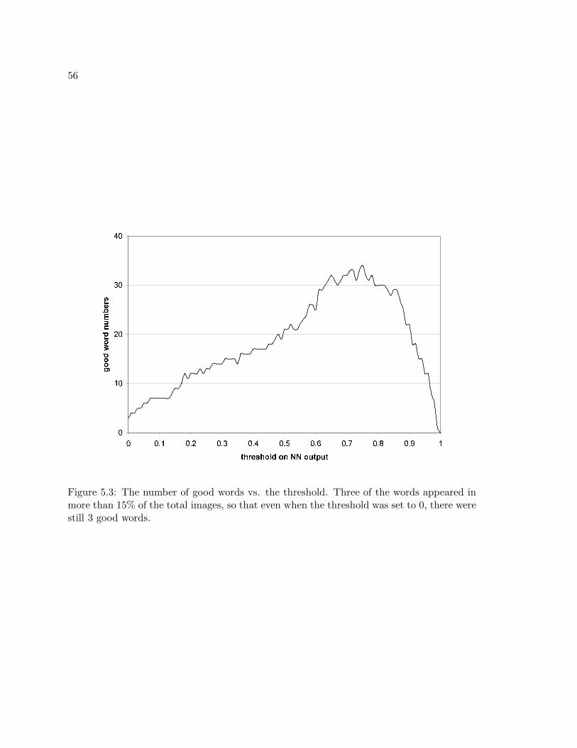
56
�
��
��
��
��
� ��� ��� ��� ��� ��� ��� �� �� ��� �
��������������� ��
���������������
Figure 5.3: The number of good words vs. the threshold. Three of the words appeared inmore than 15% of the total images, so that even when the threshold was set to 0, there werestill 3 good words.

57
Figure 5.4: Samples from the groundtruth image set.
5.2.4 Performance on Groundtruth Data Set
As several CBIR researchers have pointed out, the Corel image set is “easy” for image
retrieval tasks [50] [11] since the images are nicely grouped into different themes, the within-
group similarity is very high and in most cases, the theme object or objects occupy most of
the image and appear close to the center. We are more interested in images for which the
target object can be anywhere in the image and is not necessarily the main theme of the
image. For example, we want to recognize the category “tree” in images whose main theme
is “house”, “beach”, or “flower”, rather than only in images whose main theme is “tree”.
Our groundtruth image set contains 1,224 images and continues to grow. The set includes
our own images and those contributed by other researchers around the world. The whole
image set is free for research purpose and is fully labelled.1.
Figure 5.4 shows some sample images from the groundtruth database. There are 31
elementary object categories represented in this database: beach, boat, bridge, building, bush,
car, cherry tree, cloud, flower, football field, frozen lake, grass, ground, hill, house, stadium,
lake, lantern, mountain, people, pole, river, rock, sidewalk, sky, snow, stone, street, track,
tree, and water. There are also 20 high-level concepts: Asian city , Australia, Barcelona,
1http://www.cs.washington.edu/research/imagedatabase/groundtruth/

58
campus, Cannon Beach, Columbia Gorge, European city, Geneva, Green Lake, Greenland,
Indonesia, indoor, Iran, Italy, Japan, park, San Juans, spring flowers, Swiss mountains,
and Yellowstone. European city is a superset of Barcelona, Geneva and Italy, and Asian city
is a superset of Indonesia and Japan. Table 5.5 shows the ROC scores in ascending order
for these categories obtained using color, texture, and structure features. In general, the
lower scores are obtained for object classes that have both high variance in appearance and
insufficient samples in the database to learn those variations. Although “people” was one
of our categories, we do not claim to have a robust people-finding algorithm. Since we have
no features expressly designed for recognizing people, they are probably being recognized
mostly by context.
Figure 5.5 gives top five results for some object classes and Figure 5.6 shows some
annotation samples. High score (greater than 50) labels and “true” labels are listed for
each sample image and “true” labels are shown in boldface fonts. Sometimes, the computer
predicted labels can capture those overlooked by humans. For example, “park” is one label
the computer predicted for the first image in Figure 5.6, but it was not a “true” label in the
human-generated ground truth. This shows the situation in which computer can be more
consistent in image labelling and can help people to do a better job. The second image on
the second row in Figure 5.6 shows that our system “recognize” some objects by context.
There is no features in our system suitable for recognizing boats, but the computer predicts
boats based on the context, like the existence of blue water.
5.2.5 Performance of the Structure Feature
To more thoroughly investigate the performance of our structure feature, we created a
database of 1,951 images from freefoto.com including 1,013 images of buses, 609 images of
houses and other buildings, and 329 images of skyscrapers. Our structure features come
from consistent line clusters, which are collections of line segments having similar colors
on both sides of the segment, similar orientations, and similar locations in the image. For
these experiments we used 10 attributes for the structure features including the number of

59
Table 5.5: Groundtruth Experiments
Object Class ROC Score Object Class ROC Score
street 60.4 stone 87.1
people 68.0 hill 87.4
rock 73.5 mountain 88.3
sky 74.1 beach 89.0
ground 74.3 snow 92.0
river 74.7 lake 92.8
grass 74.9 frozen lake 92.8
building 75.4 japan 92.9
cloud 75.4 campus 92.9
boat 76.8 barcelona 92.9
lantern 78.1 geneva 93.3
australia 79.7 park 94.0
house 80.1 spring flowers 94.4
tree 80.8 columbia gorge 94.5
bush 81.0 green lake 94.9
flower 81.1 italy 95.1
iran 82.2 swiss mountains 95.7
bridge 82.7 sanjuans 96.5
car 82.9 cherry tree 96.9
pole 83.3 indoor 97.0
yellowstone 83.7 greenland 98.7
water 83.9 cannon beach 99.2
indonesia 84.3 track 99.6
sidewalk 85.7 football field 99.8
asian city 86.7 stadium 100.0
european city 87.0

60
Figure 5.5a: Top 5 results for (top row) Asian city, (second row) cannon beach, (third row) Italy, and (bottom row) park.

61
Figure 5.5b: Top 5 results for (top row)sky, (second row) spring flowers, (third row) tree, and (bottom row) water.

62
tree(97.3), bush(91.6),
spring flowers(90.3),
flower(84.4), park(84.3),
sidewalk(67.5),
grass(52.5), pole(34.1)
sky(99.8), Columbia gorge(98.8),
lantern(94.2), street(89.2),
house(85.8), bridge(80.8), car(80.5),
hill(78.3), boat(73.1), pole(72.3),
water(64.3), mountain(63.8),
building(9.5)
sky(99.2), cherry tree(98.3),
grass(88.5), tree(85.2),
sidewalk(72.9),
lantern(54.8),
water(52.3), campus(45.9)
building(99), tree(97.9),
Japan(93.3), Asian(91.2),
Columbia gorge(87.1),
bridge(79.8), Iran(73.5),
bush(65.7), grass(53.5),
sky(0.2)
sky(95.1), Iran(89.3),
house(88.6), building(80.1),
boat(71.7), bridge(67.0),
water(13.5), tree(7.7)
Italy(99.9), grass(98.5), sky(93.8),
rock(88.8), boat(80.1), water(77.1),
Iran(64.2), stone(63.9), bridge(59.6),
European(56.3), sidewalk(51.1),
house(5.3)
tree(99.9), sidewalk(95.8),
bush(95.7), grass(92.5),
ground(76.9), park(69.6),
house(5.5)
Iran(91.7), sky(85.6),
grass(75.4), Indonesia(75.0),
Asian(55.7), house(53.5),
beach(51.1), people(18.0)
Figure 5.6a: Groundtruth data set annotation samples. The labels with score higher than 50 and all human-annotatedlabels are listed for each sample image. The boldface labels are true or human-annotated labels.

63
Cannon beach(98.7), sky(98.6),
sidewalk(98.3), tree(98.1),
flower(90.6), car(89), building(88.5),
house(85.7), people(85.3), street(82.4),
bush(79.4), pole(68.4),
spring flowers(60.8)
European(98.6),
Barcelona(95.6),
building(94.2),
people(78.4), street(65.6)
European(100),
building(100),
Barcelona(99.9),
Iran(54.5)
tree(100), sky(92.9),
water(71.8), cloud(67.8),
Geneva(57.8), boat(57.3),
beach(51.1),
Australia(14.5)
building(94.8), sky(87), campus(64.5),
car(62.6), European(58.6), barcelona(53.5),
street(50.8), ground(50.5),
sidewalk(2.5), tree(5.9)
people(96.5), Geneva(65),
European(54.1) ,
building(28.3), water(7.4)
people(97.6),
indoor(87),
building(78.2)
Husky stadium(99.7),
football field(99.6),
people(99.4), track(98.4),
sky(77.2), house(72.4)
Figure 5.6b: Groundtruth data set annotation samples.

64
Table 5.6: Structure Experiments
bus house/building skyscraper
structure (%) 90.0 78.7 88.7
structure + color (%) 92.4 85.3 92.6
structure* + color (%) 94.0 86.0 91.9
(* color pair attributes were removed from the structure feature)
line segments, the colors on both sides of the segments, the main orientation, the number
of heavily overlapped segments (normalized), and the maximum number of intersections
formed with line segments from other clusters (normalized). We tested the structure feature
alone and combined with the color feature. Table 5.6 shows the ROC scores for the three
categories. While the structure feature did a pretty good job of identifying the categories,
the addition of the regions from a color segmentation of the whole image improved the
identification of the house and building category. We also tried an experiment in which
the color pair attributes were removed from the structure feature and the reduced set of
attributes were combined with the color segmentation features. The scores obtained were
very similar to the structure plus color segmentation scores shown in the table. Some top
ranked result samples for bus, houses and buildings, and skyscrapers are listed in Figure 5.7.
5.2.6 Performance on Aerial Video Frames
We applied our learning framework to recognize objects in aerial video frames. While
tracking can detect objects in motion, our object recognition system can provide information
about the static objects, such as forest, road, and field, which are also important in video
analysis. The aerial image set contains 828 video frames. Some sample images are shown
in Figure 5.8. We chose a set of 10 objects that appeared in at least 30 images for our
experiments; the object classes were airplane, car, dirt road, field, forest, house, paved road,

65
bus
houses and buildings
skyscrapers
Figure 5.7: Top ranked result samples for bus, houses and buildings, and skyscrapers
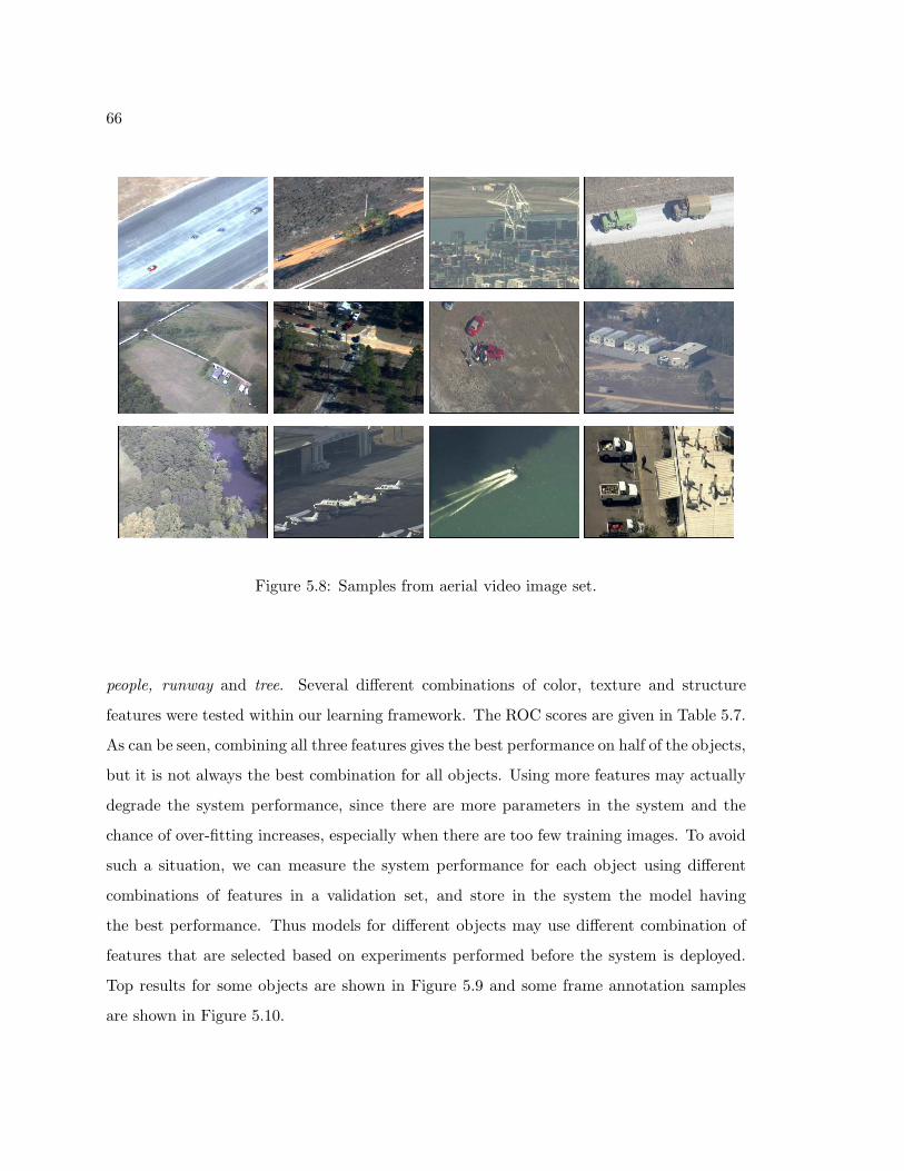
66
Figure 5.8: Samples from aerial video image set.
people, runway and tree. Several different combinations of color, texture and structure
features were tested within our learning framework. The ROC scores are given in Table 5.7.
As can be seen, combining all three features gives the best performance on half of the objects,
but it is not always the best combination for all objects. Using more features may actually
degrade the system performance, since there are more parameters in the system and the
chance of over-fitting increases, especially when there are too few training images. To avoid
such a situation, we can measure the system performance for each object using different
combinations of features in a validation set, and store in the system the model having
the best performance. Thus models for different objects may use different combination of
features that are selected based on experiments performed before the system is deployed.
Top results for some objects are shown in Figure 5.9 and some frame annotation samples
are shown in Figure 5.10.
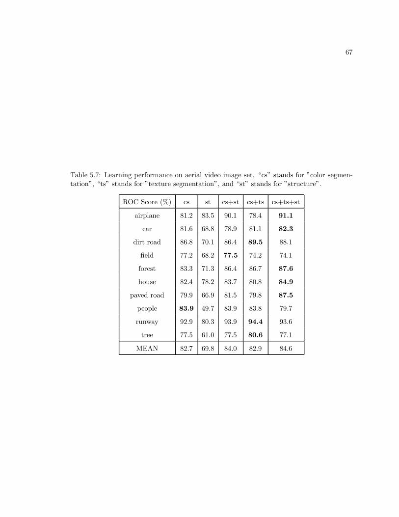
67
Table 5.7: Learning performance on aerial video image set. “cs” stands for ”color segmen-tation”, “ts” stands for ”texture segmentation”, and “st” stands for ”structure”.
ROC Score (%) cs st cs+st cs+ts cs+ts+st
airplane 81.2 83.5 90.1 78.4 91.1
car 81.6 68.8 78.9 81.1 82.3
dirt road 86.8 70.1 86.4 89.5 88.1
field 77.2 68.2 77.5 74.2 74.1
forest 83.3 71.3 86.4 86.7 87.6
house 82.4 78.2 83.7 80.8 84.9
paved road 79.9 66.9 81.5 79.8 87.5
people 83.9 49.7 83.9 83.8 79.7
runway 92.9 80.3 93.9 94.4 93.6
tree 77.5 61.0 77.5 80.6 77.1
MEAN 82.7 69.8 84.0 82.9 84.6

68
Figure 5.9: Top 6 results for airplane (row 1), dirt road (row 2), field (row 3), runway (row 4), and tree (row 5).

69
forest(94.4), house(64.1),
car(46.5), dirt road(23.4), paved
road(4.8), tree(2.3), airplane(1.5),
runway(0.0), field(0.0), people(0.0)
runway(100.0), field(98.7), car(96.2),
people(10.0), airplane(2.7), paved
road(2.4), forest(0.8), house(0.5), dirt
road(0.4), tree(0.0)
car(94.3), dirt road(91.7), field(16.2),
tree(14.2), paved road(5.3), air-
plane(5.2), people(3.9), forest(0.5),
house(0.5), runway(0.4)
runway(100.0), car(99.2), field(98.1),
dirt road(92.1), house(85.2), tree(19.4),
paved road(5.8), airplane(3.6), for-
est(2.9), people(0.1)
runway(100.0), car(99.8), field(99.3),
paved road(18.3), people(13.1),
tree(8.7), airplane(7.9), forest(1.7),
house(0.1), dirt road(0.1)
car(97.9), forest(94.2), paved
road(85.0), dirt road(72.9), tree(68.8),
airplane(39.1), house(33.2), peo-
ple(13.0), field(2.4), runway(0.0)
Figure 5.10: Aerial video frames annotation samples. Those boldface labels are true labels or human annotated labels.

70
Our system generates satisfactory results on this aerial video image set without using
any image features particularly designed for aerial images. With our open framework and
with tuned aerial image feature detectors, even better performance is expected.
5.3 Summary
We have described a new two-phase generative/discriminative learning algorithm for object
recognition in CBIR. The generative phase normalizes the description length of images,
which can have an arbitrary number of abstract region features. The discriminative step
learns which images, as represented by this fixed-length description, contain the target
object. We have compared our new method to our previous EM-variant approach, to the
ALIP approach [29], and to the machine translation approach [13] with favorable results. We
have run additional experiments with several different combinations of features on several
different image data sets. This method is for image classification, but not for localization. It
is suitable for CBIR systems, but not for other applications such as surveillance or robotics.
In the next chapter, we will show a probabilistic mechanism for localization that identifies
the regions within an image where the target object is likely to lie.

71
Chapter 6
LOCALIZATION
Our algorithms were designed for CBIR systems, not for more general object recognition
systems in which the location of the object in the image is required. However, since the
probabilities computed by our system are based on abstract regions, we can analyze the
learning procedure to determine which regions are most important in the decision-making
process. The localization procedure described in this chapter assumes that those regions
that contribute most to the decision of whether an object has a high probability of being
in an image are most likely to contain that object. In Section 6.1, we will formalize our
approach using only a single feature type, and in Section 6.2 we will extend the analysis to
take advantage of multiple feature types.
6.1 Single-Feature Case
Recall the description of the two-phase learning algorithm in Section 5.1.1. To calcuate
the probability that image Ii contains target object o using feature a, the generative step
finds those clusters, {ma}, in the feature vector space for feature a that are most likely
to appear in images containing the target object o. Then for image Ii and its type-a
region feature vector, Xai,r, we calculate the joint probability of region r and cluster ma,
P (Xai,r,m
a). From these probabilities, {P (Xai,r,m
a), r = 1, 2, . . . , nai ,m = 1, 2, . . . ,M}, we
compute a feature indicating the degree to which a component ma explains the image Ii,
Y ma
Ii= P (Ii,m
a) = f({P (Xai,r,m
a)|r = 1, 2, . . . , nai }, by an aggregate function, f . For
image Ii and type-a components {ma}, we produce the following feature vector:
Y 1a:Ma
Ii= [Y 1a
Ii, Y 2a
Ii, · · · , Y Ma
Ii]
In the discriminative step, this feature vector is fed into the trained MLP, and the output

72
indicates the probability that image Ii contains target object o.
For notational purposes, we define two terms,
Y 1a:Ma
Ii|ma=0 = [Y 1a
Ii, · · · , Y (m−1)a
Ii, 0, Y
(m+1)a
Ii, · · · , Y Ma
Ii] (6.1)
and
Y 1a:Ma
Ii|ma=P (ra,ma) = [Y 1a
Ii, · · · , Y (m−1)a
Ii,min(P (Xa
i,r,ma), Y ma
Ii), Y
(m+1)a
Ii, · · · , Y Ma
Ii] (6.2)
The MLP output using (6.1) as input calculates the likelihood of having object o in image Ii
if there is no region in Ii contributing to component ma of feature type a. The MLP output
using (6.2) as input calculates the likelihood of having object o in image Ii if only region ra
in image Ii contributes to component ma. The difference between the outputs of the MLP
with these two different inputs, MLP(
Y 1a:Ma
Ii|ma=P (ra,ma)
)
and MLP(
Y 1a:Ma
Ii|ma=0
)
, rep-
resents the contribution of region ra to the MLP output through component m. The min
function in the definition of Y 1a:Ma
Ii|ma=P (ra,ma) is to control the contribution of region ra
to component m not to exceed the value of component m from the combining function.
The contribution, Car , of region ra to the MLP output through all the components is then
calcuated by
Car =
M∑
m=1
(MLP (Y 1a:Ma
Ii|ma=P (ra,ma)) − MLP (Y 1a:Ma
Ii|ma=0))
We assume the more a region r contributes to the MLP output, the more like that r
corresponds to the target object. Figure 6.1 shows some results of locating the “cherry
tree” object by this approach using only the color segmentation feature.
6.2 Multiple-Feature Case
As described in Section 5.1.2, for multiple feature types, A = {ak, k = 1, . . . ,K}, the input
to the MLP is a concatenated feature vector:

73
Original Color Segmentation Localization
Figure 6.1: Localization of “cherry tree” object using color segmentation feature. Theprobability of a region belonging to the “cherry tree” class is shown by the brightness ofthat region.

74
Y AIi
= [Y 1a1 :Ma1
Ii, Y 1a2 :Ma2
Ii, · · · , Y 1aK :MaK
Ii]
= [Y 1a1
Ii, Y 2a1
Ii, · · · , Y Ma1
Ii, Y 1a2
Ii, Y 2a2
Ii, · · · , Y Ma2
Ii, · · · , Y 1aK
Ii, Y 2aK
Ii, · · · , Y MaK
Ii]
For notational purposes, we define
Y AIi|ma=0 = [Y 1a1 :Ma1
Ii, · · · , Y 1a:Ma
Ii|ma=0, · · · , Y 1aK :MaK
Ii] (6.3)
and
Y AIi|ma=P (ra,ma) = [Y 1a1 :Ma1
Ii, · · · , Y 1a:Ma
Ii|ma=P (ra,ma), · · · , Y 1aK :MaK
Ii] (6.4)
Similar to the single-feature case, the MLP output using (6.3) as input calculates the like-
lihood of having object o in image Ii if there is no type a region in Ii contributing to
type a component ma. The MLP output using (6.4) as input calculates the likelihood of
having object o in image Ii if only region ra in image Ii contributes to the type a compo-
nent ma. The difference between the outputs of the MLP with these two different inputs,
MLP(
Y AIi|ma=P (ra,ma)
)
and MLP(
Y AIi|ma=0
)
, represents the contribution of type a region
ra to the MLP output through the component ma of type a. To use multiple features to
locate objects, our algorithm works on the pixel level. Suppose a pixel, p, belongs to a region
rap for type a, the contribution of pixel p to the MLP output through all the components of
all the feature types is defined by
CAp =
∑
a∈A
Ma∑
ma=1
(MLP (Y AIi|ma=P (ra
p ,ma)) − MLP (Y AIi|ma=0))
Intuitively, the contribution of a pixel p to the MLP output is a summary of the con-
tributions of the different region types to which it belongs. Figure 6.2 shows some results
of locating “cheetah” objects by this approach using the Blobworld region feature and the
mean shift region feature. The second column shows the Blobworld regions detected from
the original images, and the third column shows the contribution summary through only

75
the Blobworld components. The fourth column shows the mean shift regions detected from
the original images, and the fifth column shows the contribution summary through only the
mean shift components. The last column shows the contribution summary through both
Blobworld components and mean shift components. In the localization demonstration im-
ages, the brighter the pixel value, the higher the contribution summary to the MLP output
or the higher the probability of belonging to the object. The first three rows in Figure 6.2(a)
demonstrate the situation where both features help to localize the object. The last two rows
demonstrate the situation where the Blobworld region feature is more useful. The first two
rows in Figure 6.2(b) demonstrate the situation where the mean shift region feature cannot
localize the object, but the Blobworld region feature can. The next row demonstrates the
opposite situation where the Blobworld region feature cannot localize the object, but the
mean shift region feature can. The last row demonstrates the situation where the Blob-
world region feature incorrectly localize the object, but the mean shift region feature helps
to correct it.
Figure 6.3 shows some results of locating “bus” objects by this approach using the
color segmentation region feature and the structure region feature. The second column
shows the color segmentation regions detected from the original images, and the third
column shows the contribution summary through only the color region components. The
fourth column shows the line structures detected from the original images, and the fifth
column shows the contribution summary through only the structure components. The
last column shows the contribution summary through both color region components and
structure components. The examples in Figure 6.3(a) demonstrate the situation where both
features help to localize the object. While the structure feature found the line structures,
the color region feature caught the characteristic bus colors, for example, red. The first row
in Figure 6.3(b) demonstrates the situation where the structure feature cannot localize the
object, but the color region feature can. The other rows demonstrate the opposite situation
where the color region feature cannot localize the object, but the structure feature can.
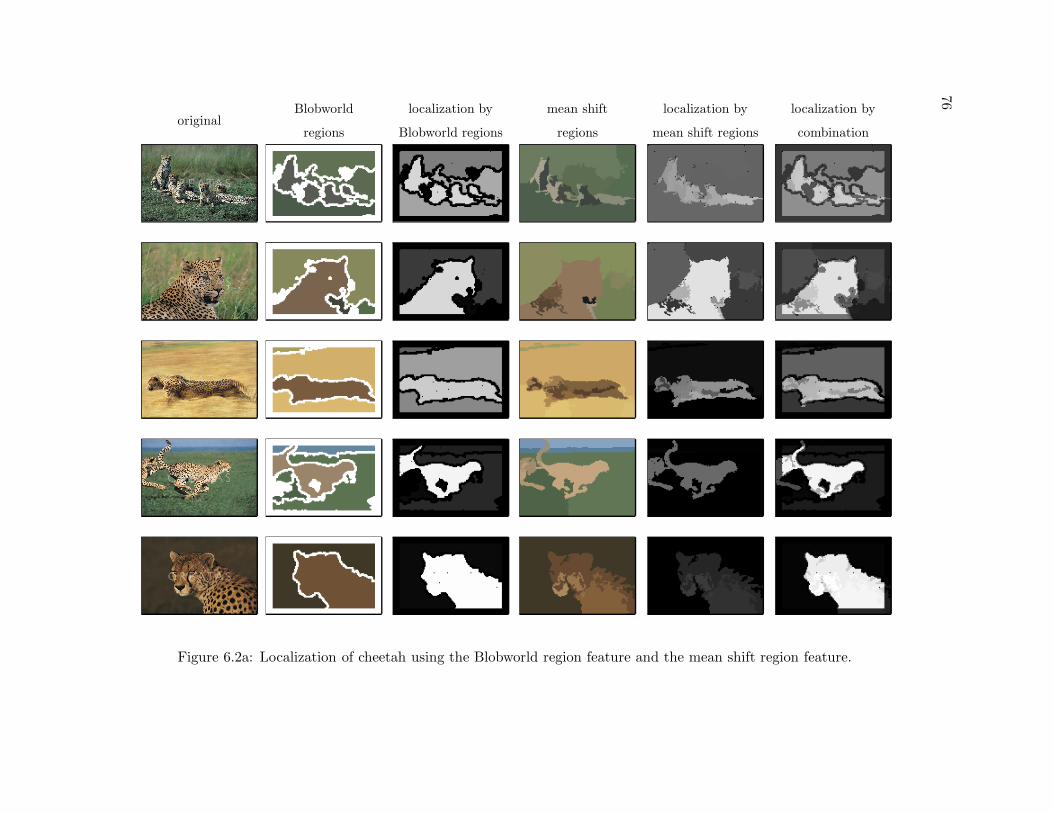
76original
Blobworld
regions
localization by
Blobworld regions
mean shift
regions
localization by
mean shift regions
localization by
combination
Figure 6.2a: Localization of cheetah using the Blobworld region feature and the mean shift region feature.

77
originalBlobworld
regions
localization by
Blobworld regions
mean shift
regions
localization by
mean shift regions
localization by
combination
Figure 6.2b: Localization of cheetah using the Blobworld region feature and the mean shift region feature.

78original
color segmentation
regions
localization by
color regionsstructure
localization by
structure regions
localization by
combination
Figure 6.3a: Localization of bus using the color segmentation region feature and the line structure feature.

79
originalcolor segmentation
regions
localization by
color regionsstructure
localization by
structure regions
localization by
combination
Figure 6.3b: Localization of bus using the color segmentation region feature and the line structure feature.

80
6.3 Summary
Although our algorithms were not designed for object localization, our analysis of the con-
tribution to the MLP output of regions or pixels allows us to provide an approximate
estimation of the target object location.

81
Chapter 7
CONCLUSIONS
Early CBIR systems searched for images based on their global appearances. This kind
of approach requires users to provide a sample image first, and the image retrieval task
is performed based on low-level image features, but not on the actual objects found in
the image. We believe a practical, user-friendly CBIR system must operate on the same
semantic level as its human users. Since humans classify images according to their objects
and concepts, the system must have the ability to recognize object and concept classes in
order to automate the process of image annotation. However, object recognition is still
an open field for computer vision research, and most successful object recognition systems
only work for some particular objects or object classes. Our main contributions to our goal
include:
• We proposed a uniform feature representation, abstract regions, to allow our system
framework to accept many different kinds of image features. This multiple-feature-
enabled approach is important for a CBIR system dealing with images representing a
wide range of objects and concepts.
• Our algorithm does not require the training images to be pre-segmented in order to
learn the object models. This is not only a relief for the data preparation, but it is
also important for system extendability, since there is little effort required to add new
object models and new image features to our system. We developed an EM-variant
algorithm for classification, using only the image label information to learn the object
models. We showed that the EM variant is able to break the symmetry in the initial
solution. We extended the EM-variant, which models an object as a single Gaussian
distribution, to Gaussian mixture models. The extension performs better on object

82
classes with high variance or multiple appearance subclasses. We developed a two-
phase algorithm that handles multiple features in a unified way. We have compared it
to two published systems with favorable results. We have run additional experiments
with several different combinations of features on several different image data sets
including a large 60K COREL image set.
• We added the object localization ability to our system, so that it can provide the
probable location of an object in an image.
There are some problems worthy of further exploration. One is how to find the optimal
clusters in a feature space. The quality of the clustering procedure is important, since it will
effect the efficiency and the accuracy of our system. Other forms of combining functions are
worth examining. Spatial relationship between regions are also an important cue for object
recognition. How to combine spatial relationships into our system, especially with multiple
features, deserves further research.

83
BIBLIOGRAPHY
[1] Jeffrey R. Bach, Charles Fuller, Amarnath Gupta, Arun Hampapur, Bradley Horowitz,Rich Humphrey, Ramesh Jain, and Chiao-Fe Shu. Virage image search engine: an openframework for image management. In Proceedings of SPIE - The International Societyfor Optical Engineering, volume 2670, pages 76–87, 1996.
[2] Kobus Barnard and David Forsyth. Learning the semantics of words and pictures. InInternational Conference on Computer Vision, volume 2, pages 408–415, 2001.
[3] A. P. Berman and L. G. Shapiro. A flexible image database system for content-basedretrieval. Computer Vision and Image Understanding, 75(1-2):175–195, 1999.
[4] A. Del Bimbo, P. Pala, and S. Santini. Visual image retrieval by elastic deformationof object sketches. In IEEE Symposium on Visual Languages, pages 216–223, 1994.
[5] J. Canny. A computational approach to edge detection. In IEEE Transactions onPattern Analysis and Machine Intelligence, volume 8, pages 679–698, 1986.
[6] Chad Carson, Serge Belongie, Hayit Greenspan, and Jitendra Malik. Blobworld: Imagesegmentation using expectation-maximization and its application to image querying.PAMI, 24(8):1026–1038, 2002.
[7] Chad Carson, Megan Thomas, Serge Belongie, Joseph M. Hellerstein, and JitendraMalik. Blobworld: A system for region-based image indexing and retrieval. In ThirdInternational Conference on Visual Information Systems. Springer, 1999.
[8] Yizong Cheng. Mean shift, mode seeking, and clustering. PAMI, 17:790–799, August1995.
[9] D. Comanicu and P. Meer. Mean shift: A robust approach toward feature spaceanalysis. PAMI, 24:603–619, May 2002.
[10] M. S. Costa and L. G. Shapiro. 3D object recognition and pose with relational indexing.Computer Vision and Image Understanding, 79(3):364–407, 2000.
[11] T. Deselaers, D. Keysers, and H. Ney. Classification error rate for quantitative evalua-tion of content-based image retrieval systems. In International Conference on PatternRecognition, volume II, pages 505–508. IEEE Computer Society, 2004.

84
[12] Thomas G. Dietterich, Richard H. Lathrop, and Toms Lozano-Prez. Solving the mul-tiple instance problem with axis-parallel rectangles. Artificial Intelligence, 89:31 – 71,1997.
[13] P. Duygulu, K. Barnard, J.F.G. de Freitas, and D.A. Forsyth. Object recognition asmachine translation: Learning a lexicon for a fixed image vocabulary. In ECCV02,volume 4, pages 97–112, 2002.
[14] Choi E. and Hall P. Data sharpening as a prelude to density estimation. Biometrika,86:941–947(7), December 1999.
[15] A. Etamadi. Robust segmentation of edge data. In Proceedings of the IEE ImageProcessing Conference, 1992.
[16] R. Fergus, P. Perona, and A. Zisserman. Object class recognition by unsupervisedscale-invariant learning. In CVPR 2003, pages 264–271, 2003.
[17] Margaret M. Fleck, David A. Forsyth, and Chris Bregler. Finding naked people. InProceedings of the European Conference on Computer Vision (ECCV) (2), pages 593–602, 1996.
[18] M. Flickner, H. Sawhney, W. Niblack, J. Ashley, Q. Huang, and B. Dom et al. Queryby image and video content: the qbic system. IEEE Computer, 28(9):23–32, 1995.
[19] D. Forsyth and M. Fleck. Body plans. In Proceeding of IEEE Conference on ComputerVision and Pattern Recognition, pages 678–683, 1997.
[20] D. Forsyth, J. Mundy, A. Zisserman, C. Coelho, A. Heller, and C. Rothwell. Invariantdescriptors for 3-d object recognition and pose. IEEE Transactions on Pattern Analysisand Machine Intelligence, 13(10):971–991, 1991.
[21] D.A. Forsyth and M.M. Fleck. Automatic detection of human nudes. IJCV, 32(1):63–77, August 1999.
[22] K. Fukunaga and L. Hostetler. The estimation of the gradient of a density function,with applications in pattern recognition. Information Theory, IEEE Transactions on,21:32– 40, Jan 1975.
[23] Yihong Gong. Advancing content-based image retrieval by exploiting image color andregion features. Multimedia Systems, 7(6):449–457, 1999.

85
[24] A. R. Hanson and E. M. Riseman. Computer Vision Systems, chapter VISIONS: AComputer System for Interpreting Scenes, pages 303–333. Academic Press, a. hansonand e. riseman, eds. edition, 1978.
[25] D. P. Huttenlocher and S. Ullman. Recognizing solid objects by alignment with animage. International Journal of Computer Vision, 5(2):195–212, 1990.
[26] J. Jeon, V. Lavrenko, and R. Manmatha. Automatic image annotation and retrievalusing cross-media relevance models. In Proceedings of SIGIR ’03 Conference, pages119–126, 2003.
[27] T. Kadir and M. Brady. Saliency, scale and image description. IJCV, 45(2):83–105,November 2001.
[28] A. Kuehnle. Symmetry-based recognition of vehicle rears. Pattern Recognition Letters,12(4), 1991.
[29] J. Li and J.Z. Wang. Automatic linguistic indexing of pictures by a statistical modelingapproach. PAMI, 25(9):1075–1088, September 2003.
[30] Y. Li, J. Bilmes, and L. G. Shapiro. Object class recognition using images of abstractregions. In Proceedings of the International Conference on Pattern Recognition. IEEEComputer Society, 2004.
[31] Y. Li, J. Bilmes, and L. G. Shapiro. A generative/discriminative learning algorithmfor object recognition in content-based image retrieval. In CVPR (submitted). IEEEComputer Society, 2005.
[32] Y. Li and L. G. Shapiro. Consistent line clusters for building recognition in cbir. InProceedings of the International Conference on Pattern Recognition, volume 3, pages952–6, 2002.
[33] Wei-Ying Ma and B. S. Manjunath. Netra: A toolbox for navigating large imagedatabases. Multimedia Systems, 7(3):184–198, 1999.
[34] Oded Maron and Aparna Lakshmi Ratan. Multiple-instance learning for natural sceneclassification. In ICML, 1998.
[35] Sharad Mehrotra, Yong Rui, Michael Ortega, and Thomas S. Huang. Supportingcontent-based queries over images in MARS. In International Conference on Multime-dia Computing and Systems, pages 632–633, 1997.

86
[36] M.Turk and A.Pentland. Eigen faces for recognition. Journal of Cognitive Neuroscience,3(1), 1991.
[37] H. Murase and S.K. Nayar. Visual learning and recognition of 3-d objects from ap-pearence. International Journal of Computer Vision, 14:5–24, 1995.
[38] Apostol Natsev, Rajeev Rastogi, and Kyuseok Shim. WALRUS: a similarity retrievalalgorithm for image databases. In Proc. SIGMOD, pages 395–406, 1999.
[39] A. Pentland, R. Picard, and S. Sclaroff. Photobook: Content-based manipulation ofimage databases. In SPIESRIVD II, 1994.
[40] Henry A. Rowley, Shumeet Baluja, and Takeo Kanade. Neural network-based facedetection. IEEE Transactions on Pattern Analysis and Machine Intelligence, 20(1):23–38, 1998.
[41] S. Sclaroff and A. P. Pentland. Object Recognition and Categorization Using ModalMatching. In Proc. of 2nd CAD-Based Vision Workshop, pages 258–265, 1994.
[42] Jianbo Shi and Jitendra Malik. Normalized cuts and image segmentation. IEEE Trans-actions on Pattern Analysis and Machine Intelligence, 22(8):888–905, 2000.
[43] A. W. M. Smeulders, M. Worring, S. Santini, A. Gupta, and R. Jain. Content-basedimage retrieval at the end of the early years. IEEE Transactions on Pattern Analysisand Machine Intelligence, 22(12):1349–1380, 2000.
[44] J. R. Smith and C. S. Li. Image classification and querying using composite regiontemplates. Computer Vision and Image Understanding: Special Issue on Content-Based Access of Image and Video Libraries, 75(1-2):165–174, 1999.
[45] John R. Smith and Shih-Fu Chang. Visualseek: A fully automated content-based imagequery system. In ACM Multimedia, pages 87–98, 1996.
[46] John R. Smith and Shih-Fu Chang. Image and video search engine for the world wideweb. In Storage and Retrieval for Image and Video Databases (SPIE), pages 84–95,1997.
[47] A. Vailaya, A. K. Jain, and H.-J. Zhang. On image classification: City images vs.landscapes. Pattern Recognition, 31:1921–1936, 1998.
[48] James Ze Wang, Jia Li, and Gio Wiederhold. SIMPLIcity: Semantics-sensitive inte-grated matching for picture LIbraries. IEEE Transactions on Pattern Analysis andMachine Intelligence, 23(9):947–963, 2001.

87
[49] Markus Weber, Max Welling, and Pietro Perona. Unsupervised learning of models forrecognition. In Proceedings of the European Conference on Computer Vision (ECCV)(1), pages 18–32, 2000.
[50] Thijs Westerveld and Arjen P. de Vrie. Experimental evaluation of a generative prob-abilistic image retrieval model on ’easy’ data. In Proceedings of the Multimedia Infor-mation Retrieval Workshop 2003, 2003.
[51] Gnther Wyszecki and W. S. Stiles. Color Science : Concepts and Methods, QuantitativeData and Formulae. Wiley-Interscience, second edition, 2000.
[52] T. Zielke, M. Brauckmann, and W. Von Seelen. Intensity and edge-based symmetrydetection with an application to car-following. CVGIP: Image Understanding, 58(2),1993.

88
VITA
Yi Li received BS and MS degree in Computer Science from Peking University, P. R.
China, in 1995 and 1998, respectively and MS degree in Computer Science from University
of Washington in 2000. He joined Lucent Technology from 2000 to 2002. He received PhD
degree in Computer Science from University of Washington in 2005. His research interests
include content-based image retrieval, computer vision, pattern recognition and machine
learning.