OASIS FINANCIAL MODULE - dhvptdf78rzwk.cloudfront.net · OASIS FINANCIAL MODULE Authors: Peter Taylor, Johanna Carter – Oasis Loss Modelling Framework Ltd

OASIS FINANCIAL MODULE Authors: Peter Taylor, Johanna Carter – Oasis Loss Modelling Framework Ltd.

© Oasis LMF, 2016. Course developed by Oasis LMF in conjunction with Imperative Space and the Institute for Environmental Analytics.

1

This document sets out the methods and options for calculating ground-up losses, and the way

insurance policy terms and conditions are applied in the “Oasis Financial Module”. This is the

principal function of the Oasis “Kernel”. The Oasis “Kernel” additionally includes the

management of technical processes for webservices, generation of instructions to execute data

inputs, the “Financial Module” calculations, and outputs.

The Oasis Loss Modelling Framework uses a philosophy for loss calculations which reflects its

origins within the insurance industry. This philosophy differs considerably from approaches

found in most other catastrophe loss modelling software, so consideration is given to

comparing and contrasting Oasis with the popular methods and why it is to be expected that

Oasis will express uncertainty more adequately. There will be many cases where the

differences in methodology may not be material, but there will be plenty where it is, especially

when it comes to quantifying uncertainties and the effect these uncertainties have on price and

capital.

WHY THIS MATTERS

Perhaps the most important reason for reading this paper is help everyone see how catastrophe

loss models calculate their numbers. Whilst there are client-confidential analyses of “financial

modules” by the main providers, they are not published openly nor, to our knowledge, has

there been any critique of their inadequacies.

Financial calculations only matter if they make a difference in pricing, allocating capital, or

managing a business. Oasis’s Financial Module is a high fidelity tool that portrays a richer

insight into risk as well as showing up the errors inherent in simplifications in common use.

By providing both a conceptual framework and set of practical tools, users, management and

regulators can challenge vendor modelling companies and help them raise their game.

BACKGROUND

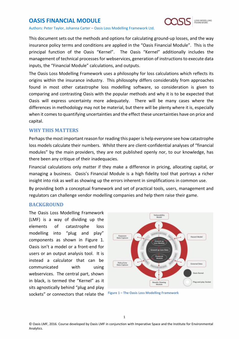
The Oasis Loss Modelling Framework

(LMF) is a way of dividing up the

elements of catastrophe loss

modelling into “plug and play”

components as shown in Figure 1.

Oasis isn’t a model or a front-end for

users or an output analysis tool. It is

instead a calculator that can be

communicated with using

webservices. The central part, shown

in black, is termed the “Kernel” as it

sits agnostically behind “plug and play

sockets” or connectors that relate the Figure 1 – The Oasis Loss Modelling Framework



2

external actualised model and business data to the abstract structures used for the calculations.

The Oasis LMF is a “framework” in that it provides structures within which particular solutions

can be developed to solve particular problems. The “plug-and-play” connections to models and

user input and outputs are one of the elements of generality in the LMF; the other is the way

that financial calculations are done. In designing the methods and options for the calculation,

four considerations were incorporated:

• Non-parametric probability distributions. Modelled and empirical intensities and

damage responses can show significant uncertainty, sometimes multi-modal (that is

there can be different peaks of behaviour rather than just a single central behaviour).

Moreover, the definition of the source insured interest (e.g. property) location and

characteristics (such as occupancy and construction) can be imprecise. The associated

values for event intensities and consequential damages can therefore be varied and

their uncertainty can be represented in general as probability distributions rather than

point values1. The design of Oasis therefore makes no assumptions about the

probability distributions and instead treats all probability distributions as probability

masses in discrete bins, including using closed interval point bins such as the values [0,0]

for no damage and [1,1] for total damage. Thus Oasis uses histograms (also termed

“discrete” or “binned”) probability distributions. How this is done is described below.

• Monte-Carlo sampling. Insurance practitioners are used to dealing with losses arising

from events. These losses are numbers, not distributions, and policy terms are applied

to the losses individually and then aggregated and further conditions or reinsurances

applied. Oasis takes the same perspective, which is to generate individual losses from

the probability distributions and the way to achieve this is random sampling called

“Monte-Carlo” sampling from the use of random numbers (as if from a roulette wheel)

to solve equations that are otherwise intractable.

• Correlation of intensity and of damage across coverages and locations. Correlations

are typically modelled between coverages and between locations. Let’s take these in

turn. For coverages at a single location, the question is whether damage between, say,

buildings and contents, is correlated. Models often just fully correlate in the sense of

using the same random numbers to sample the distributions for coverages at a

property. A more sophisticated way is to use a regression correlation coefficient and

generate random numbers using pairwise correlation coefficients. These coefficients

are often relatively easy to estimate from claims data and the degree of correlation

expressed in terms of a correlation coefficient. Another way to handle the correlation

of damage could be to take a primary distribution (such as buildings) and sample that

and then apply a correlation matrix for the damage to another coverage given the

sampled damage from the primary distribution. This does not require separate

1 Having said that, Oasis works with many models some of which are purely point estimates (mean) of intensity. Some models use parametric (“closed-form”) continuous distributions, and some use histogram binned distributions. Many use a combination of continuous and point (Dirac delta function) probability distributions.



3

sampling of the related distributions. It is mathematically equivalent to correlated

sampling. Another route is to extend the conditional calculation by allowing a

probability distribution (not just a value) to depend on the primary distribution.

Business interruption, for example, can be modelled as a probability distribution

conditional on property (buildings and contents damage).

For locations, the most obvious correlation is likely to be that variations in intensity are

likely to be lower for adjacent properties and independent if they are far apart. It is also

arguable that vulnerability (leading to damage) might be correlated locally if, say,

systemic variations in building practice occurred in a location due to the same builder.

These two are intensity correlation and vulnerability correlation. It is even conceivable

that the combination of intensity and vulnerability might be related as with a failure of

flood defences in which case intensity and vulnerability are correlated. A complex

matter, to be sure, but of potentially large financial consequence. Oasis supports all

these variations one way or another as described in APPENDIX D, but the onus falls

increasingly on the model provider and the use of APIs where location correlations are

concerned.

• Data-driven Application of Insurance Terms and Conditions. As well as the agnostic

approach to ground-up losses, Oasis LMF also uses its agnostic approach for policy terms

and conditions. Whether insurance or reinsurance the variations and complexities are

endless. For insurance, though, they fall into three types of process – iterative

aggregation to a “level”, application of rules to determine the element of loss that is

insured, and then back-allocation to lower levels for processing to the next “level”.

Reinsurance is more complicated as there can be inuring policies from which a particular

reinsurance benefits – and not just simple inuring policies, in actual fact there are often

very complex reinsurance programme structures. The modelling of these complex cases

is not intended to be covered in Release 1 of Oasis, though simple event-based inurings

and many layered facultative reinsurances can be handled. Application of Oasis to

complex reinsurance programmes will be covered in Release 2, but they are described

below in brief anyhow.

ALTERNATIVE APPROACHES

The methods chosen by Oasis are general and cover most cases known in other financial

modelling methods (albeit using discrete numeric calculations in place of closed-form

continuous functions). However, quite different methods are commonly used today in other

vendor and internally developed modelling software so it is worth explaining these and

commenting on the differences that might follow if using them compared to Oasis LMF

methods.

• Source probability distributions for intensity and damage. There are many ways in

which different models represent event footprint intensity and associated damage.

Some just provide mean values (simply mean damage models); others provide full



4

probability distributions for both intensity and vulnerability. Many use point values for

intensity coupled with damage (vulnerability) distributions. Most use parametric

distributions for damage. For example, a popular catastrophe loss model uses one of

beta, gamma, or beta-Bernoulli depending on the peril; others such as flood models use

uniform distributions for flood intensity and truncated normal for damage; earthquake

models popularly use truncated lognormal for intensity and beta for damage. A few

allow fully histogramic distributions, especially for vulnerability. There are sometimes

peculiar, and arguably erroneous, reasons behind these choices and significant

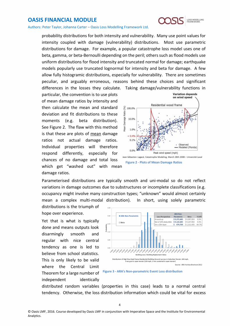
differences in the losses they calculate. Taking damage/vulnerability functions in

particular, the convention is to use plots

of mean damage ratios by intensity and

then calculate the mean and standard

deviation and fit distributions to these

moments (e.g. beta distribution).

See Figure 2. The flaw with this method

is that these are plots of mean damage

ratios not actual damage ratios.

Individual properties will therefore

respond differently, especially for

chances of no damage and total loss

which get “washed out” with mean

damage ratios.

Parameterised distributions are typically smooth and uni-modal so do not reflect

variations in damage outcomes due to substructures or incomplete classifications (e.g.

occupancy might involve many construction types; “unknown” would almost certainly

mean a complex multi-modal distribution). In short, using solely parametric

distributions is the triumph of

hope over experience.

Yet that is what is typically

done and means outputs look

disarmingly smooth and

regular with nice central

tendency as one is led to

believe from school statistics.

This is only likely to be valid

where the Central Limit

Theorem for a large number of

independent identically

distributed random variables (properties in this case) leads to a normal central

tendency. Otherwise, the loss distribution information which could be vital for excess

Figure 2 - Plots of Mean Damage Ratios

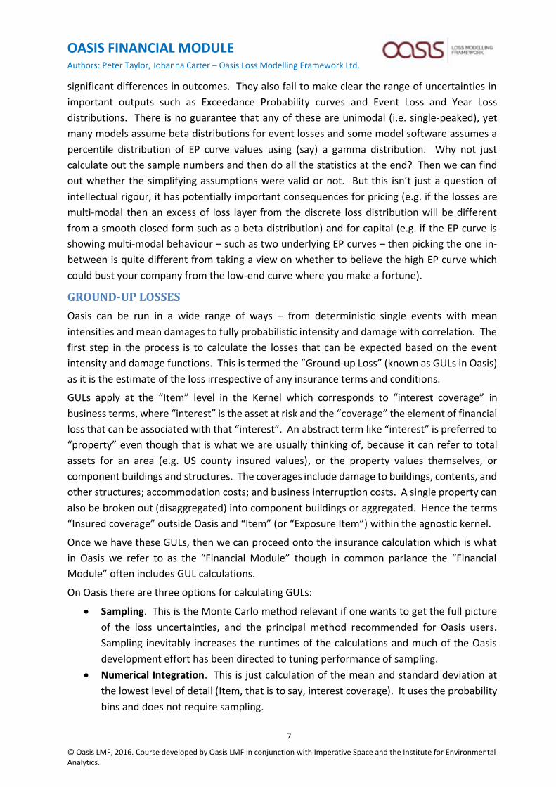
Figure 3 - ARA's Non-parametric Event Loss distribution



5

of loss calculations gets washed out before the policy terms can be applied. The

companies using recognised uncertainty in the source distributions will be better

equipped to understand the likelihood of loss, price and capital needs of the full loss

distributions giving them an arbitrage advantage. One model that does use full

vulnerability distributions is Applied Research Associates (ARA) in their HurLoss model.

The diagram from their sales brochure shown in Figure 3 illustrates the advantage of

better information: the true bi-modal distribution results in a significantly different price

for an excess layer versus its smooth, parameterized counterpart.

• Calculation of losses. The alternatives are to compute out all possible probability

combinations and then combine them (sometimes termed “convolution”) or to pick

some metrics, such as a mean and standard deviation, and calculate these using

numerical integration and then assume some closed form distribution. Further terms

and conditions would then be applied to the closed form distribution. For example, the

incomplete beta distribution for deductibles and limits if the beta distribution had been

chosen for the closed form distribution of ground-up losses by event. It only takes a

little reflection to see that following through sampled losses as if they were actual losses

is closer to what happens, more versatile, and more accurate for the many complex

terms and conditions that apply in insurance. The downsides are that it is

computationally intensive and the numbers are statistical not numerically integrated so

an important factor is taking sufficient samples relative to a desired precision of

calculation. Oasis has written a paper on this question - “Sampling Strategies and

Convergence”, available on the Oasis website. Whether the full uncertainty approach

of Oasis will make any difference to numbers affecting underwriting depends on the

problem and the metrics of interest. This is especially relevant whenever there are

excess of loss conditions as the assumptions of closed form (e.g. beta) distributions of

event losses can be sensitive to the

model. As a general rule, large

numbers of homogenous properties

(e.g. residential treaties) will give

convergent answers so uncertainty

may not matter as much, whereas for

commercial property the uncertainty

is very likely to affect the results. This

is exemplified in the “Robust

Simulation” approach advocated by

ImageCat as shown in Figure 4.

• Correlations. Correlations are typically modelled between coverages and between

locations. Let’s take these in turn. For coverages, Oasis provides a range of options

from totally correlated to independent sampling to dependent coverages from a

primary coverage. Any model that does not include correlations for coverages will give

Figure 4 - ImageCat's Robust Simulation EP Curves



6

very different results if they should be used. So a model that assumes independence

will give lower, and much lower where there are large spreads on uncertainty,

accumulated results than one with fully dependent correlations. For locations,

correlations can come from hazard intensity and/or vulnerability as described above.

Location correlation can, again, cause a major increase in losses compared to assuming

no correlation. Many models, though, do not use any location correlation but instead

calculate the moments (means and standard deviations) and then aggregate across

exposures by computing out the means and correlated standard deviations (as the sum

of the standard deviations) and uncorrelated standard deviations (as the square root of

the sum of the variances). This approach can be done in Oasis in a similar way for full

uncertainty correlating all locations. However, with Oasis it is possible to define groups

of locations and their correlation. See APPENDIX D for further discussion of how Oasis

handles correlations.

• “Events, dear boy, events”. A famously alleged response of Harold Macmillan to a

journalist when asked what is most

likely to blow governments off course.

The same could be said of insurance and

reinsurance companies! Appropriately

termed the “primary uncertainty”, the

catalogue of events and their severity

and distribution over time is the basis of

catastrophe modelling. Yet vendor

modellers can be cavalier in event set

generation and subsequent “boiling down” to small event sets able to fit the

computational constraints of their loss models. Karen Clark, founder of AIR, spotted

this clearly when she founded Karen Clark & Co and produced “Characteristic Events”

based on physical return periods and

then applying hundreds of them – for

example for US hurricane - for a given

return period over the United States.

The results were shocking; they

revealed the high variability of portfolio

losses to the choice of landfalling event

(see Figure 5 from KKC). It gets worse –

the fewer the events the wider the

underlying (and currently hidden to

most cat modellers) uncertainties in the Exceedance Probability curves used to estimate

Value at Risk capital for Solvency II (Figure 6 from Oasis).

These differences can matter. Assumptions for closed form intensity and vulnerability

distributions, paucity of event catalogues, and simplifications over correlations can all induce

Figure 6 - Example portfolio losses for hurricane landfall Characteristic Events

Figure 5 - Dispersion of EP curves (Oasis Toy Model)



7

significant differences in outcomes. They also fail to make clear the range of uncertainties in

important outputs such as Exceedance Probability curves and Event Loss and Year Loss

distributions. There is no guarantee that any of these are unimodal (i.e. single-peaked), yet

many models assume beta distributions for event losses and some model software assumes a

percentile distribution of EP curve values using (say) a gamma distribution. Why not just

calculate out the sample numbers and then do all the statistics at the end? Then we can find

out whether the simplifying assumptions were valid or not. But this isn’t just a question of

intellectual rigour, it has potentially important consequences for pricing (e.g. if the losses are

multi-modal then an excess of loss layer from the discrete loss distribution will be different

from a smooth closed form such as a beta distribution) and for capital (e.g. if the EP curve is

showing multi-modal behaviour – such as two underlying EP curves – then picking the one in-

between is quite different from taking a view on whether to believe the high EP curve which

could bust your company from the low-end curve where you make a fortune).

GROUND-UP LOSSES

Oasis can be run in a wide range of ways – from deterministic single events with mean

intensities and mean damages to fully probabilistic intensity and damage with correlation. The

first step in the process is to calculate the losses that can be expected based on the event

intensity and damage functions. This is termed the “Ground-up Loss” (known as GULs in Oasis)

as it is the estimate of the loss irrespective of any insurance terms and conditions.

GULs apply at the “Item” level in the Kernel which corresponds to “interest coverage” in

business terms, where “interest” is the asset at risk and the “coverage” the element of financial

loss that can be associated with that “interest”. An abstract term like “interest” is preferred to

“property” even though that is what we are usually thinking of, because it can refer to total

assets for an area (e.g. US county insured values), or the property values themselves, or

component buildings and structures. The coverages include damage to buildings, contents, and

other structures; accommodation costs; and business interruption costs. A single property can

also be broken out (disaggregated) into component buildings or aggregated. Hence the terms

“Insured coverage” outside Oasis and “Item” (or “Exposure Item”) within the agnostic kernel.

Once we have these GULs, then we can proceed onto the insurance calculation which is what

in Oasis we refer to as the “Financial Module” though in common parlance the “Financial

Module” often includes GUL calculations.

On Oasis there are three options for calculating GULs:

• Sampling. This is the Monte Carlo method relevant if one wants to get the full picture

of the loss uncertainties, and the principal method recommended for Oasis users.

Sampling inevitably increases the runtimes of the calculations and much of the Oasis

development effort has been directed to tuning performance of sampling.

• Numerical Integration. This is just calculation of the mean and standard deviation at

the lowest level of detail (Item, that is to say, interest coverage). It uses the probability

bins and does not require sampling.



8

• Sample 0. This gives the numerically integrated mean in sample format. It can be used

to compare sampled values to numerically integrated values but more importantly

provides a fast way to run an Oasis model all the way through Financial Module to

Output using mean damage. This can provide a valuable sense-check that the data and

policies are performing as expected before running the longer and much more data-

intensive sampling.

Getting into a position to calculate GULs requires the probability distributions for intensity and

damage. After that come the GUL calculation options for sampling and numerical integration.

Generation of Probability Distributions for use in Oasis

Given that the Kernel uses binned distributions, it is necessary to relate a modeller’s

representation of uncertainty to the Kernel’s discrete distributions.

Spreadsheets on the Oasis Members’ website and the Oasis “Data Interfaces” specification

provide examples of how this works, but in summary it involves four processes – defining the

bin structures; generating the event footprint intensity probability distributions; generating the

vulnerability probability distributions; and handling correlations. The first three are described

in the Oasis “Data Interfaces” specification and in APPENDIX A of this paper.

Correlations are handled in a number of ways in Oasis, but the simplest involves relating the

choice of random numbers for sampling the coverages and locations. 100% correlations and

pairwise correlations (e.g. between buildings and contents) can be specified in the load of

exposures (using the GROUP_ID column and populating the correlation input file). Correlations

between hazard intensities (if probabilistic) or between vulnerabilities (if probabilistic) are

handled in Oasis using external modeller-supplied APIs (e.g. as webservices); there are no

standard methods for correlations such as copulas that anyone wishes to use. This may change.

In the absence of deciding correlation rules by location (which are nearly always important),

Oasis, in common with other models, can calculate full correlation and full independence. Oasis

does it stochastically rather than by summing variances (for independence) or standard

deviations (full correlation).

“Full Uncertainty”

It is tempting to think that by using these probability distributions we are tackling most of the

uncertainties in catastrophe models. But this is not so. As explained in APPENDIX D we not

only have the “primary uncertainty” of event frequency but also many other contributions most

of which loss models do not and cannot reflect.

It is not that helpful simply to say that each insurer or reinsurer should allow for these additional

uncertainties, but that is often all we can say within models and the important issue is to

recognise the limitations of our knowledge using models.

Fixed Reference Models and Dynamic Sub-models

Oasis R1.5 can used pre-defined tables or API sources of model data



9

Pre-defined pre-calculated reference model tables for event footprints and vulnerability

matrices (and their associated probability distributions) involves defining and pre-loading

model files once and then use of the model just looks up the relevant data from these (often

large) tables, usually with a further pre-process to define the “Effective Damageability”

distribution (see below).

APIs support dynamic definition of the model (e.g. webservice or filter queries) to generate only

those model files that are needed for the properties being modelled. This can massively reduce

the cardinality of the event footprint and vulnerability matrix tables, which in some cases would

be otherwise impractically large, but also allows more complex and IP-protected rules to be

provided by the model supplier and maintained as their own code. These APIs can be called

from a front-end to Oasis and also from the Kernel.

APPENDIX B describes the API-based “Sub-model” strategy which is one of the strategies

explored in the separate Oasis “Sub-model” paper. They are all variants of the precept

“generate the sub-model from the exposures (properties) instead of applying the exposures to

the already generated general model”.

We expect models will in time move entirely over to “Sub-model” strategies rather than today’s

most common approach of pre-calculated event footprints and vulnerabilities.

Approaches to Sampling

There are four principal ways sampling can achieved within Oasis:

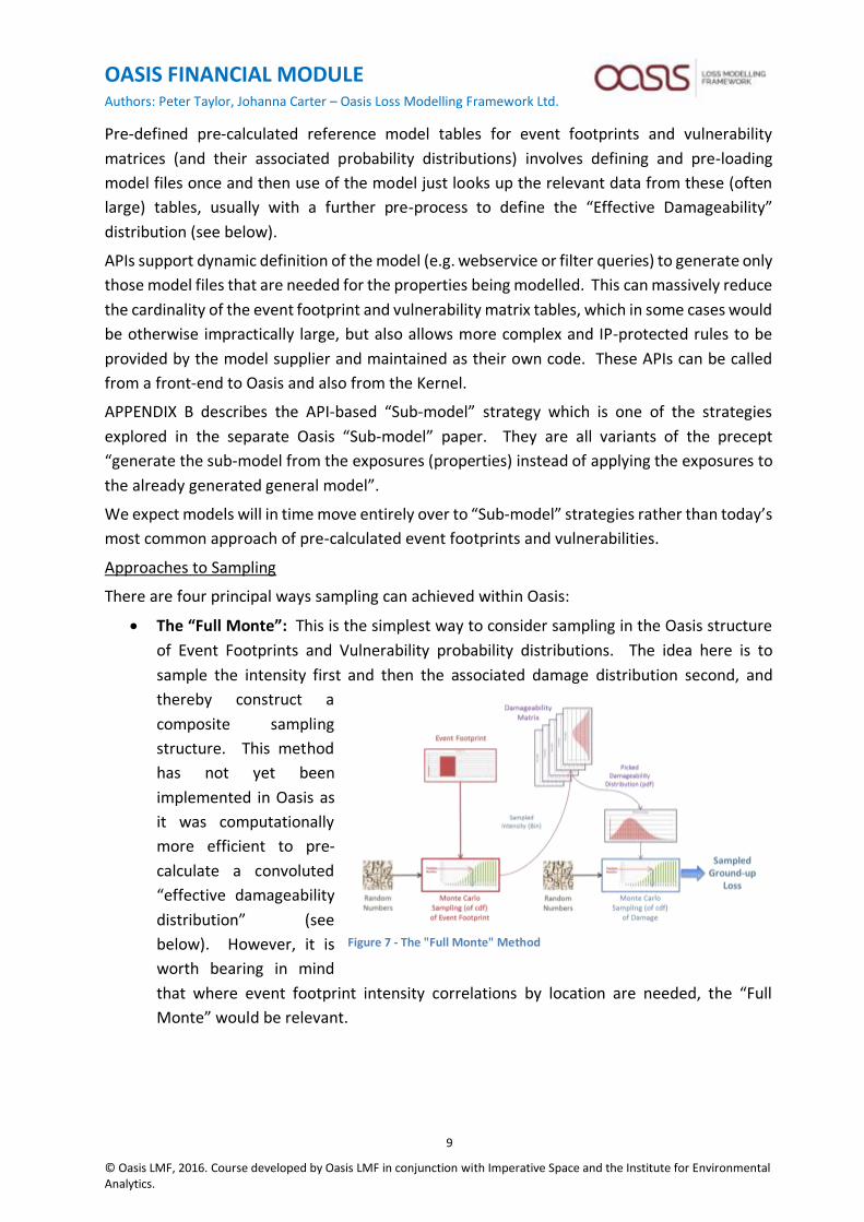
• The “Full Monte”: This is the simplest way to consider sampling in the Oasis structure

of Event Footprints and Vulnerability probability distributions. The idea here is to

sample the intensity first and then the associated damage distribution second, and

thereby construct a

composite sampling

structure. This method

has not yet been

implemented in Oasis as

it was computationally

more efficient to pre-

calculate a convoluted

“effective damageability

distribution” (see

below). However, it is

worth bearing in mind

that where event footprint intensity correlations by location are needed, the “Full

Monte” would be relevant.

Figure 7 - The "Full Monte" Method



10

• Effective Damageability Distributions: this is the method currently in use in R1.1 and

R1.5 of Oasis. It pre-computes a

single cumulative distribution

function (CDF) for the damage by

“convolving” the binned intensity

distribution with the vulnerability

matrices (shown in Figure 8 as a

family of “Damage State

Distributions”).

Sampling can then be done against

the single CDF rather than twice as

in the “Full Monte” as shown in

Figure 9 which also shows how we do the convolution. We compute the probability

masses (termed the “pdf”, probability density function) first then construct the CDF.

Because in many cases there is a

standard set of event footprint and

damageability combinations (e.g. for

a particular area) and the

computation of CDFs can be

computationally laborious, then

“Benchmark” CDFs can be pre-

computed and additional

distributions are generated

incrementally when a portfolio of

exposures is applied. For instance,

there might be a portfolio which is

primarily for Yorkshire, but there are

a couple of properties included from Lancashire. Then using the Yorkshire Benchmark

makes sense and the few properties from Lancashire get their additional CDFs at

runtime.

Figure 8 - Effective Damageabilty - The Idea

Figure 9 - Effective Damageability Method



11

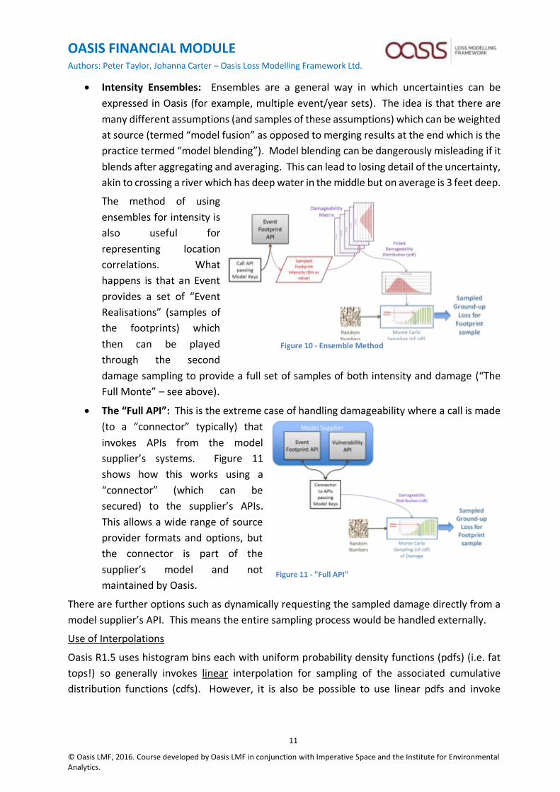
• Intensity Ensembles: Ensembles are a general way in which uncertainties can be

expressed in Oasis (for example, multiple event/year sets). The idea is that there are

many different assumptions (and samples of these assumptions) which can be weighted

at source (termed “model fusion” as opposed to merging results at the end which is the

practice termed “model blending”). Model blending can be dangerously misleading if it

blends after aggregating and averaging. This can lead to losing detail of the uncertainty,

akin to crossing a river which has deep water in the middle but on average is 3 feet deep.

The method of using

ensembles for intensity is

also useful for

representing location

correlations. What

happens is that an Event

provides a set of “Event

Realisations” (samples of

the footprints) which

then can be played

through the second

damage sampling to provide a full set of samples of both intensity and damage (“The

Full Monte” – see above).

• The “Full API”: This is the extreme case of handling damageability where a call is made

(to a “connector” typically) that

invokes APIs from the model

supplier’s systems. Figure 11

shows how this works using a

“connector” (which can be

secured) to the supplier’s APIs.

This allows a wide range of source

provider formats and options, but

the connector is part of the

supplier’s model and not

maintained by Oasis.

There are further options such as dynamically requesting the sampled damage directly from a

model supplier’s API. This means the entire sampling process would be handled externally.

Use of Interpolations

Oasis R1.5 uses histogram bins each with uniform probability density functions (pdfs) (i.e. fat

tops!) so generally invokes linear interpolation for sampling of the associated cumulative

distribution functions (cdfs). However, it is also be possible to use linear pdfs and invoke

Figure 10 - Ensemble Method

Figure 11 - "Full API"



12

quadratic sampling of cdfs. APPENDIX E describes these options and the reduction of

discretisation errors that can be assisted with quadratic sampling.

Methods of Random Number Sampling

As described in the Oasis “Sampling Strategies and Convergence” paper, there are more

strategies for sampling than simple “brute force” random numbers taken uniformly from the

interval [0,1]. These include stratified and antithetic sampling which can in some cases

dramatically reduce the number of samples needed to achieve convergence.

There are further options such as use of SOBOL random numbers (see, for example,

http://people.sc.fsu.edu/~jburkardt/py_src/sobol/sobol.html) which can achieve similar

benefits by reducing the “white space” between random numbers. Oasis R1 uses only “brute

force” but does allow pre-defined tables of random numbers so it would be easy to implement

SOBOL sequences and stratified and antithetic sampling.

Numerical Integration

It is commonly asked why Oasis doesn’t just use numerical integration and, as has already been

explained, this is because the application of policy terms and conditions can be very complex

and is usually highly non-linear (“excess of loss” policy terms). Whilst there is a computational

cost for sampling, the benefits of applying insurance structures easily outweighs it especially as

it means assumptions need not be made about the output event loss tables.

Oasis nonetheless provides an option to compute mean, variance and standard deviations for

each location coverage called “Analytics” in Oasis. The usual statistical tricks can then be

applied to them to construct aggregated means and correlated and uncorrelated aggregate

standard deviations. These “Analytics” run very quickly so if one wished to assume a beta

distribution for location coverage event losses and either use that for policy calculations and

re-sample from that (as at least one modelling company does). From an Oasis philosophy,

though, it would be absurd to lose or mask the uncertainty information (see Outputs section

below).

OASIS FINANCIAL MODULE (Policy Terms and Conditions)

Applying Policy Terms and Conditions

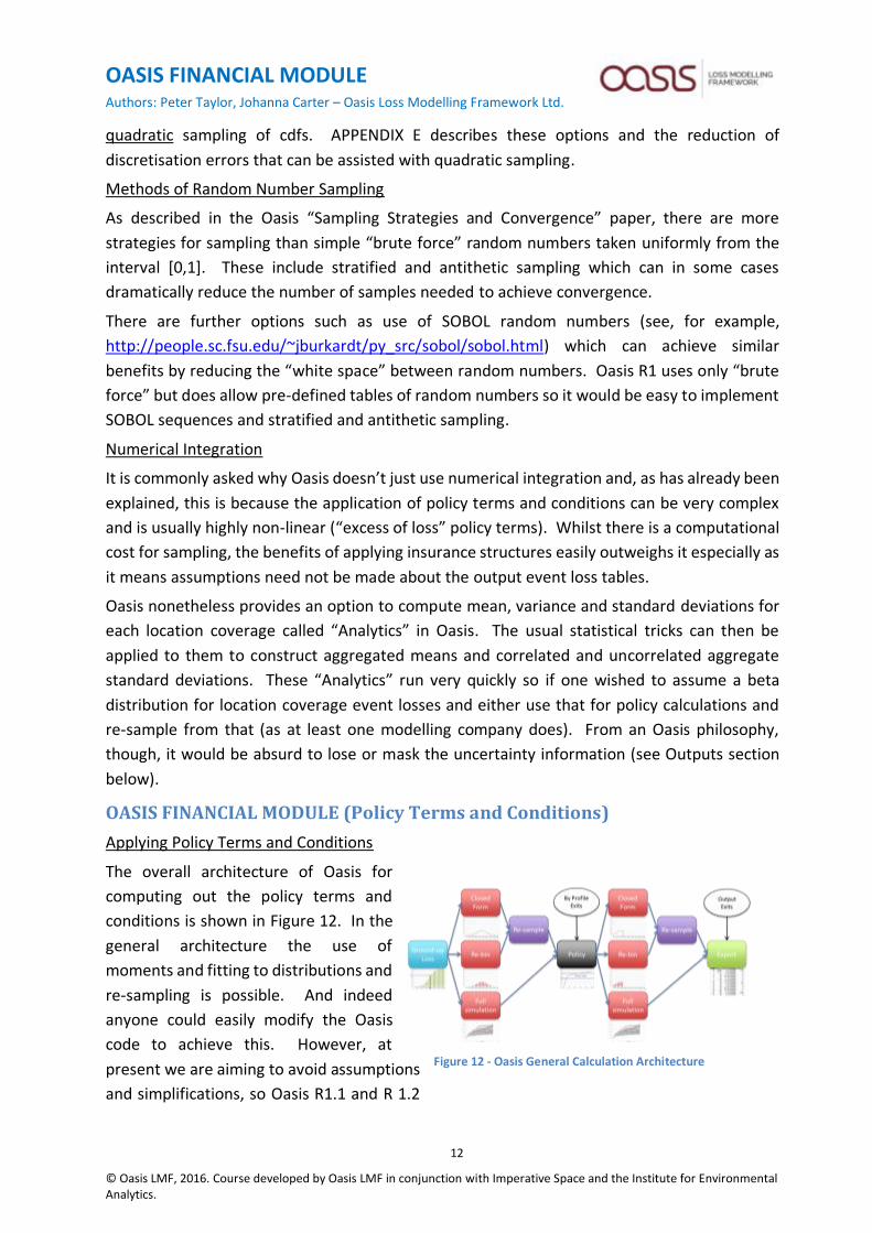
The overall architecture of Oasis for

computing out the policy terms and

conditions is shown in Figure 12. In the

general architecture the use of

moments and fitting to distributions and

re-sampling is possible. And indeed

anyone could easily modify the Oasis

code to achieve this. However, at

present we are aiming to avoid assumptions

and simplifications, so Oasis R1.1 and R 1.2

Figure 12 - Oasis General Calculation Architecture

http://people.sc.fsu.edu/~jburkardt/py_src/sobol/sobol.html



13

only provide the full sample set, which are

propagated forward to the policy terms and

conditions as if they were a large number of

event realisations. Figure 13 shows this

approach.

This can be changed for future releases if the

demand is there or if the open community

develops the code (assuming anyone wants

it!).

Insurance Structures

Insurance policies have terms and conditions applying at many different levels and with many

variations in the rule of calculation. Some of the simplest are shown to the right, but there are

many variations and the interested reader is advised to consult the Oasis website for actual

examples. Here we shall look at the structural side as that is what makes the calculations tricky.

The diagrams work from bottom to top, with the ground up losses coming in at the bottom and

the insurance losses popping out at the top:

• Simplest: this is when the ground-up losses are

accumulated to the highest level and policy terms and

conditions applied. There could be many policies

(termed “layers” in Oasis) applicable to the same

aggregation (termed a “programme” in Oasis).

• Simple: The next level of complexity is to include

coverage terms such as location coverage deductibles

(such as a buildings or contents deductible - these are

very common) and then aggregate the net figures up to

the policy level for the excess of loss. In R1.1 and R1.5

today, application of coverage terms is done separately

in FM (the “Financial Module” for the policy terms and

conditions calculations), but these may be done as part

of the ground-up loss calculation in future releases.

• Simplish: The next step is to apply location terms such as

limits, before summarising up to the location level after

coverage deductibles. The results of these calculations

are then fed up to the overall policy terms.

• Less Simple: Another stage of complication is when the

higher level is based on aggregations which have already

been suppressed in calculating a lower level. An example

Figure 13 - Oasis Release 1 Calculation Architecture

Figure 14 –Simple Insurance Structures



14

is where policy coverage deductibles and limits are

applied after location terms. Here the post-location

losses have to be “back-allocated” to the coverage

level (usually in proportion to the proportion of

coverage to the post-location losses) and then

aggregated.

• Complex: And then we have a myriad of cases where

terms and conditions apply at many levels, from location coverage to location to

locational areas (e.g. municipalities) to areas where

perils are sub-limited, to policy coverages and then to

the policy as a whole. At each level there can be

different policy terms applied. These can be very

complex indeed revealing the appetite of underwriters

to put in conditions whenever there is a loss!

FM Processing

The general way Oasis deals with these insurance structures is to follow the “level” logic and

apply iteratively. Figure 16 shows how each level is processed, with stages for:

• Unify: brings together

relevant Items to process.

• Filter: decides which of these

to include.

• Aggregate: sums up relevant

data to specified level.

• Calculate: computes

insurance recovery.

• Allocate: back-allocates to

Item level (if needed).

• Save: saves data for the next round of

processing.

There is also a greyed-out [Re-bin] option which represents the potential for re-binning if

performance was a problem.

The logic for generating the appropriate tables to drive the FM calculation is shown in an Excel

spreadsheet, the “FM Wizard” which takes the user through a series of questions to define the

structure and data values in these tables. What this amounts to is a scripting language, which

in future versions we may develop into a full “Contract Definition Language”.

In the Oasis FM, these processes are orchestrated by data tables giving information on the

levels and aggregations and allocation rules, together with back-allocation.

Figure 15 - Complex Insurance Structures

Figure 16 - FM Calculation Components



15

For details of how the data interface files are constructed to represent these structures, please

see the Oasis “Data Interfaces” specification. In brief, the Oasis Kernel for Policy Terms and

Conditions, which is termed “FM” in Oasis, needs the following four files:

• what is to be insured (the collection of exposure items, the “Programme”);

• what is being applied (the “Layer”);

• the calculation rule that applies (the “PolicyTC”); and

• the specific policy terms and condition values and rules (“Profile”).

In addition, there can be a dictionary for Programme and Account details called Prog which, in

conjunction with Layer, provides the composite key of a policy in Oasis.

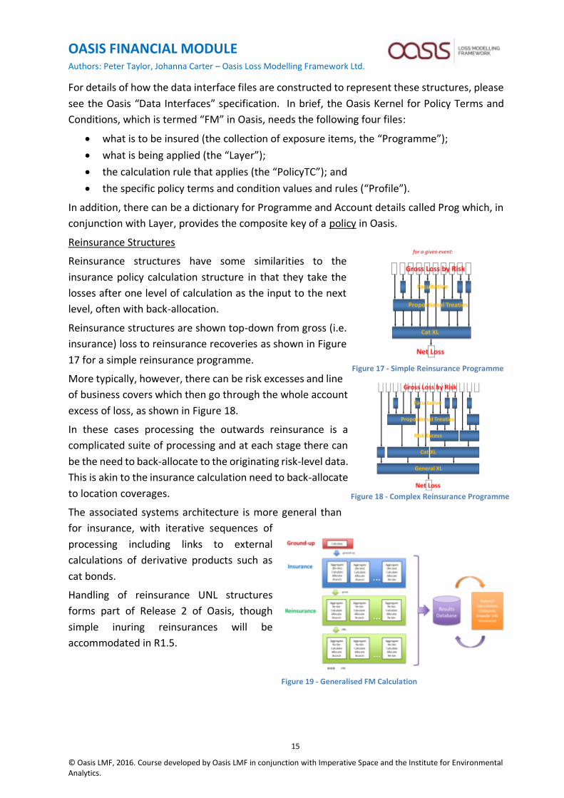
Reinsurance Structures

Reinsurance structures have some similarities to the

insurance policy calculation structure in that they take the

losses after one level of calculation as the input to the next

level, often with back-allocation.

Reinsurance structures are shown top-down from gross (i.e.

insurance) loss to reinsurance recoveries as shown in Figure

17 for a simple reinsurance programme.

More typically, however, there can be risk excesses and line

of business covers which then go through the whole account

excess of loss, as shown in Figure 18.

In these cases processing the outwards reinsurance is a

complicated suite of processing and at each stage there can

be the need to back-allocate to the originating risk-level data.

This is akin to the insurance calculation need to back-allocate

to location coverages.

The associated systems architecture is more general than

for insurance, with iterative sequences of

processing including links to external

calculations of derivative products such as

cat bonds.

Handling of reinsurance UNL structures

forms part of Release 2 of Oasis, though

simple inuring reinsurances will be

accommodated in R1.5.

Figure 17 - Simple Reinsurance Programme

Figure 18 - Complex Reinsurance Programme

Figure 19 - Generalised FM Calculation



16

“A theory is more impressive the greater the simplicity of its premises, the more different

types of things it relates and the more extended its areas of applicability.”

A Einstein Autobiographical Notes 33 1946



17

APPENDIX A GENERATING OASIS PROBABILITY DISTRIBUTIONS

As described in the Oasis Data Interfaces Specification paper, connectors provide the

translation of a source model’s parameterisation of event footprint intensity and vulnerability

into the kernel’s probability distributions. This Appendix provides a summary of this process

relevant to the definition of the Oasis Kernel’s calculations.

Intensity and Damage Bin structures

Probability bins are used in the Oasis Kernel for intensity and damage. At present these are

fixed bin structures (but with variable bin sizes and allowing for closed intervals) for a given

model so are part of the model definition to Oasis. Typically the intensity bins include a [0,0]

value to allow for “miss factor” and the damage bins include a [0,0] bin for no damage and a

[1,1] bin for total loss. A single point distribution can be binned to a defined structure

(depending on the way vulnerability is defined) or set as a closed interval for the single point.

Event Footprint (Hazard) probability distributions

Event footprints in Oasis are relative to definitions of Event and Location for a Peril. There are

many ways location is defined in different models such as Cresta zones, post/zipcodes, grids,

variable resolution grids, polygons, and co-ordinated cells. These vary by peril and many

models offer multiple options (e.g. Postcode or grid points) according to the availability of

exposure data. Whichever location definition is chosen for whichever peril, the list of valid

values for the combination is known in Oasis as an AreaPeril dictionary and any business front-

end system needs to pick the appropriate AreaPerilID. Multiple perils can be handled by

multiple EventIDs with an Event Dictionary identifying the common “Event”. Occurrence of an

Event can be defined with the model-specific Event Profile (e.g. as a year number) or through a

separate cross-reference table which allows the same event to be used more than once in the

Event Year set. Oasis provides options for single (scalar) metric values or binned probability

distributions. Single point values can either be binned or their value can be the bin. Multiple

metrics can be treated in the same way and applied to different coverages (e.g. buildings might

use spectral acceleration and contents use peak ground acceleration) or combined against one

coverage (provided there is an associated damageability matrix. Where data are not provided

in native Oasis format of binned probability values, a “connector” (maybe with an API if

dynamic) is needed to take the model’s view of intensity and convert it into an Oasis-

computable form.

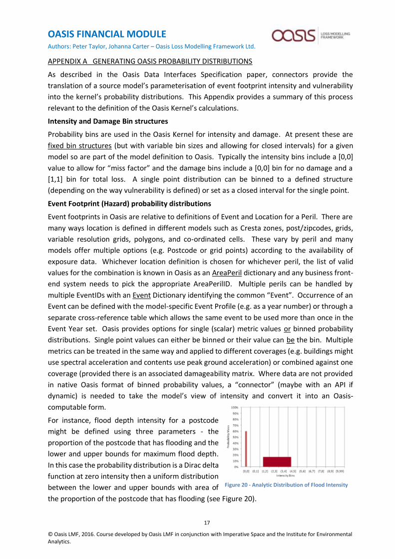
For instance, flood depth intensity for a postcode

might be defined using three parameters - the

proportion of the postcode that has flooding and the

lower and upper bounds for maximum flood depth.

In this case the probability distribution is a Dirac delta

function at zero intensity then a uniform distribution

between the lower and upper bounds with area of

the proportion of the postcode that has flooding (see Figure 20).

Figure 20 - Analytic Distribution of Flood Intensity



18

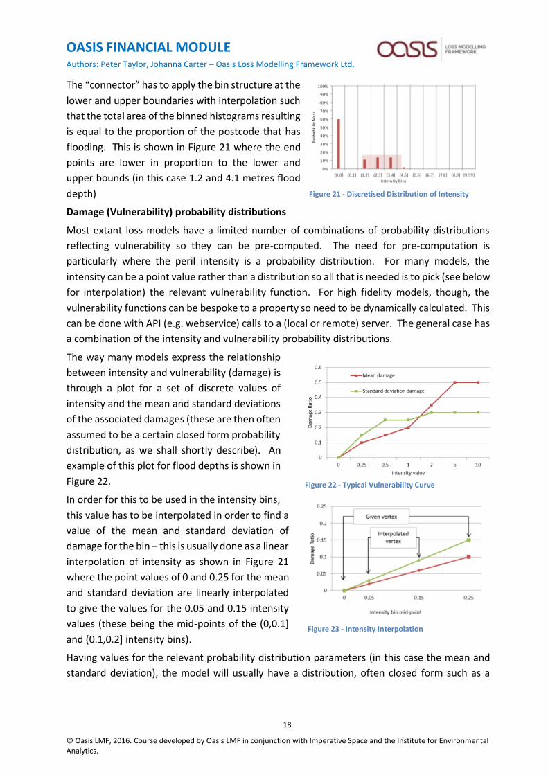
The “connector” has to apply the bin structure at the

lower and upper boundaries with interpolation such

that the total area of the binned histograms resulting

is equal to the proportion of the postcode that has

flooding. This is shown in Figure 21 where the end

points are lower in proportion to the lower and

upper bounds (in this case 1.2 and 4.1 metres flood

depth)

Damage (Vulnerability) probability distributions

Most extant loss models have a limited number of combinations of probability distributions

reflecting vulnerability so they can be pre-computed. The need for pre-computation is

particularly where the peril intensity is a probability distribution. For many models, the

intensity can be a point value rather than a distribution so all that is needed is to pick (see below

for interpolation) the relevant vulnerability function. For high fidelity models, though, the

vulnerability functions can be bespoke to a property so need to be dynamically calculated. This

can be done with API (e.g. webservice) calls to a (local or remote) server. The general case has

a combination of the intensity and vulnerability probability distributions.

The way many models express the relationship

between intensity and vulnerability (damage) is

through a plot for a set of discrete values of

intensity and the mean and standard deviations

of the associated damages (these are then often

assumed to be a certain closed form probability

distribution, as we shall shortly describe). An

example of this plot for flood depths is shown in

Figure 22.

In order for this to be used in the intensity bins,

this value has to be interpolated in order to find a

value of the mean and standard deviation of

damage for the bin – this is usually done as a linear

interpolation of intensity as shown in Figure 21

where the point values of 0 and 0.25 for the mean

and standard deviation are linearly interpolated

to give the values for the 0.05 and 0.15 intensity

values (these being the mid-points of the (0,0.1]

and (0.1,0.2] intensity bins).

Having values for the relevant probability distribution parameters (in this case the mean and

standard deviation), the model will usually have a distribution, often closed form such as a

Figure 21 - Discretised Distribution of Intensity

Figure 22 - Typical Vulnerability Curve

Figure 23 - Intensity Interpolation



19

truncated normal distribution, with truncated values going

into the end points. These are then calculated for each bin

mid-point in a “connector” as shown in the diagram to the

right. Note that the mean and standard deviation of the

resulting distribution is not the same as that of the source

distribution, and this distortion will be particularly

noticeable at the end points. The model developer should

therefore take into account the effect of truncating

unbounded distributions such as the normal or lognormal or gamma distributions when setting

the putative values of the mean and standard deviation for the truncated distributions. When

you put all this together you get a full family of damage distributions by intensity which can

then be “convolved” (weighted) by the intensity bin probabilities to create an “Effective

Damageability” distribution for the event footprint vulnerability combination (see main text).

For the many cases where intensities are point values, it is only necessary to pick the

(interpolated) damage function. For cases where there are intrinsic correlations of intensity,

then the sampling of the random numbers could be done using the “Full Monte” (see main text)

if some correlation rule could be defined or, more likely, simply call the model using an API as

we shall now describe.

Figure 24 - Truncated Normal Distribution



20

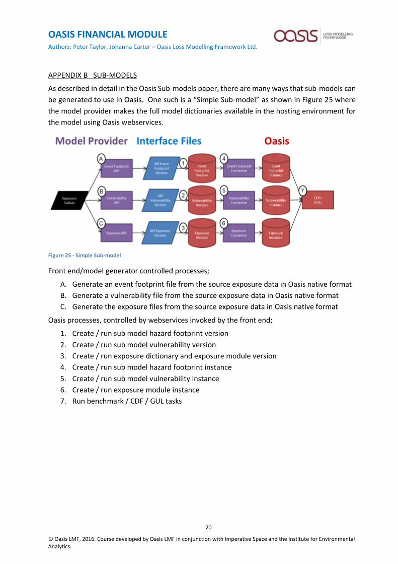
APPENDIX B SUB-MODELS

As described in detail in the Oasis Sub-models paper, there are many ways that sub-models can

be generated to use in Oasis. One such is a “Simple Sub-model” as shown in Figure 25 where

the model provider makes the full model dictionaries available in the hosting environment for

the model using Oasis webservices.

Figure 25 - Simple Sub-model

Front end/model generator controlled processes;

A. Generate an event footprint file from the source exposure data in Oasis native format

B. Generate a vulnerability file from the source exposure data in Oasis native format

C. Generate the exposure files from the source exposure data in Oasis native format

Oasis processes, controlled by webservices invoked by the front end;

1. Create / run sub model hazard footprint version

2. Create / run sub model vulnerability version

3. Create / run exposure dictionary and exposure module version

4. Create / run sub model hazard footprint instance

5. Create / run sub model vulnerability instance

6. Create / run exposure module instance

7. Run benchmark / CDF / GUL tasks



21

APPENDIX C OUTPUTS

Not strictly to do with the Financial Module, but we add a few comments about Oasis outputs

as the calculations in the kernel affect the outputs.

Figure 26 shows the

architecture – the

calculated results

are joined in SQL

queries to

reference

dictionaries

whether those used

in input such as the

AreaPeril or Event

or Exposure

dictionaries or

additional user-

defined dictionaries for the purpose of output.

The outputs from the SQL queries in the “Analysis Connectors” are stored in an “Output

Database” and can then be exported using “Export Connectors” in a format required by an

external data store.

Of the many outputs (for further details see the Oasis Outputs specification), of particular

interest are EP Curves and Event Loss Distributions.

EP Curves

The Exceedance Probability or “EP” Curve, also known as the Value At Risk or VaR curve, plots

the probability of exceeding a certain level of loss. You might have thought there was only one

way to do this, but there are many. At the most basic level, the current modelling companies

fall into two camps on this calculation. First, those who use event frequencies (arrival rates) to

calculate an “Occurrence” EP (OEP) curve or the plot of the largest loss from any one event in

a year. In this case an algorithm using arrival rates can be used readily. Second, those who use

relative frequency and event/year simulations to calculate annual losses either on an aggregate

basis called an Aggregate EP (AEP) curve, or an occurrence basis (OEP). These are calculated on

a simple relative frequency basis. The second method has genuine advantages for AEP curves

as the event occurrences by year (indeed by date) form part of the model and so can

incorporate time correlations or “clustering” of events. The former method really isn’t much

good for AEP and requires assumption of an arrival distribution such as Poisson or Negative

Binomial (which are very crude compared to the modelled correlations) and then a convolution

which usually requires Fast Fourier Transform techniques to solve numerically.

The EP curves so calculated can themselves take on several forms depending on how they are

computed.

Figure 26 - Output Architecture



22

Figure 27 shows three principal options which, as you can see, give different plots:

• EP curve of means: Take all the mean

losses and rank order them across Years

simulated

• Mean of Wheatsheaf EP curve: EP curve

of a metric of the samples (in this case the

mean of the sample EP Curves, though

could be the median, very little difference).

• Full EP curve: where each sample is treated as a

resampling of the annual events (e.g. 10 samples from 10,000 years becomes samples

from 100,000 years).

Of particular interest is the graph showing plots of

all the samples’ EP curves themselves which in

Oasis we term a “Wheatsheaf” as shown in Figure

28. What this example shows clearly is “multi-

modal” behaviour which is that the distribution of

EP curves is not simply a case of variations around a

central tendency. This is also highlighted in

ImageCat’s “Robust Simulation” approach (see

“Calculation of Losses” above).

Taking another example, in which we do see central

tendency, Figure 29 shows a large dispersion

around the mean EP curve (however this is

calculated). It is worth noting that the spread is not

a function of number of samples (it only improves

the resolution of the spread distribution). Instead

the spread of a uni-modular distribution can be

reduced by increasing the number of events or

number of similar exposures.

It is also worth noting that the Mean of the

Wheatsheaf is a good estimator to the final

distribution and, as Figure 30 shows, can differ from

the EP curve of the means (the latter being a poor

estimator). Applying policy terms to this ground-up

loss Wheatsheaf gives a different distribution as

shown in Figure 31, where the losses are capped at

the limit but break through when there are multiple

occurrences in a given year (limit assumed not

reinstateable).

Figure 27 - Comparison of EP Curves

Figure 28 – Multi-modal Wheatsheaf

Figure 29 - Wheatsheaf from a "Toy Model"

Figure 31 - EP Curves from a “Toy Model”

Figure 30 - FM Wheatsheaf



23

Event Loss Distributions

As well as EP curves, Oasis stochastic calculations reveal the underlying Event Loss histograms.

For example, Figure 32 shows the actual

distribution (in red) compared to the beta

distribution assumption (ground-up loss,

with beta distribution fitted using the

numerically integrated moments).

Ensembles

It is worth noting that these uncertainties are

only a small part of the picture. In the wider case of loss models representing reality then, as

discussed in APPENDIX F, we have many additional factors coming into play.

One way to handle some of these, in particular those that relate to uncertainties in the science

or data, is to use “ensembles” to represent epistemic (i.e. lack of knowledge) uncertainty. An

ensemble in this sense is a set of different source assumptions. To some extent this can already

be represented within the usual framework by allowing probability distributions (e.g. for

vulnerability), but it is possible to go further. Ensembles that represent different weightings of

assumptions can be played through the model to produce more complete output distributions

reflecting our beliefs about theories or knowledge of reality.

And this could, in principle, be taken further to an iterative adjustment of our beliefs based on

experience using a Bayesian framework. The ensemble output distribution can be compared

to actual results and the chance of those assumptions producing the observed output used to

adjust the assumption (prior) probabilities. Although this has not yet been done, it will be

addressed as part of an Oasis multi-model modelling Working Party in 2015.

Figure 32 - Event Loss Distribution vs Beta Distribution



24

APPENDIX D HANDLING OF CORRELATIONS IN OASIS

Correlation in the sense used for Oasis means a dependency between the sampling of one

(random) variable and that of another. For instance, if buildings and contents damage is 100%

correlated for a property, then sampling of these coverages should use the same random

number.

Oasis supports various types of correlations:

1. Random numbers (indexed by GROUPIDs), which assign random numbers to coverages

and provides options for fully correlated or fully uncorrelated.

2. Pairwise correlated random numbers (see Figure 33) In this case a Pearson Correlation

Coefficient, r, is used to use a second random number to generate a random number

that is correlated to a given random number. The method is shown in the tables below

3. Correlation matrix (not implemented in R1.5 ktools), where a multiple sampling of

random numbers is performed but from a matrix (or more generally, a hypercube) such

as a percentile correlation (copula) or rank-ordered correlation. The idea here is that

some random variables underlying the GROUPIDs have a relationship to each other such

that the random numbers are chosen for each GROUPID using a rule that relates them

together in a matrix. A way that this can work is to pick the random number for a second

variable contingent on the value sampled from the first value or, more generally,

random numbers are sampled for each variable by sampling from a copula. Further

details of what could be done can be provided, but as yet we have had no examples of

this type of correlation and there was no interest in copulas in the 2014 Correlations

Figure 33 - Pairwise Correlation



25

Working Party. However, this can be implemented by creating a variant of ktools on

R1.5.

4. Conditional values. Here, the sampling is from, say, Buildings, but the other coverages

(e.g. Contents and Business Interruption) are determined from the sampled damage

using a deterministic relationship (with suitable interpolation). This reflects the

correlations that can be obtained from loss data. An example of this has been creaed

for ARA’s model using aratools based on Oasis R1.5.

5. Conditional sampling. Here, a primary sampling is from, say, Buildings and Contents to

give Property damage and the other coverages (e.g. Business Interruption) then use a

distribution which is conditional upon the property damage.This would be delivered

using the ktools framework in R1.5.

Running Oasis for fully correlated and uncorrelated.

In many cases, though, there is no decent knowledge of the correlations due to factors such as

location. One way to deal with this is to take the basic or pairwise correlations by coverage and

then undertake these entirely independently (uncorrelated, the default) or dependently (pick

the same random numbers for all coverages in any group deemed to be correlated). All of this

can be controlled in Methods 1 and 2 by setting the GROUPID in the ITEM table and, if needed,

set the CORRELATION table as well. For instance, one might say that all properties in the same

estate are correlated but between estates they are independent.

For the second moment, a popular method is to take a linear combination of the standard

deviations of the correlated and uncorrelated losses. This is, though, largely unjustified, so

more likely better to run with and without correlation (using GROUPID) and consider the range.

Another way would be to generate an ensemble of different correlation assumptions

[Note that for fully correlated losses then the standard deviation of the sum of the variables is

the sum of the standard deviations and for fully uncorrelated, the variance of the sum of the

variables is the sum of the variances, which means the standard deviation is the square root of

the sum of the variances].



26

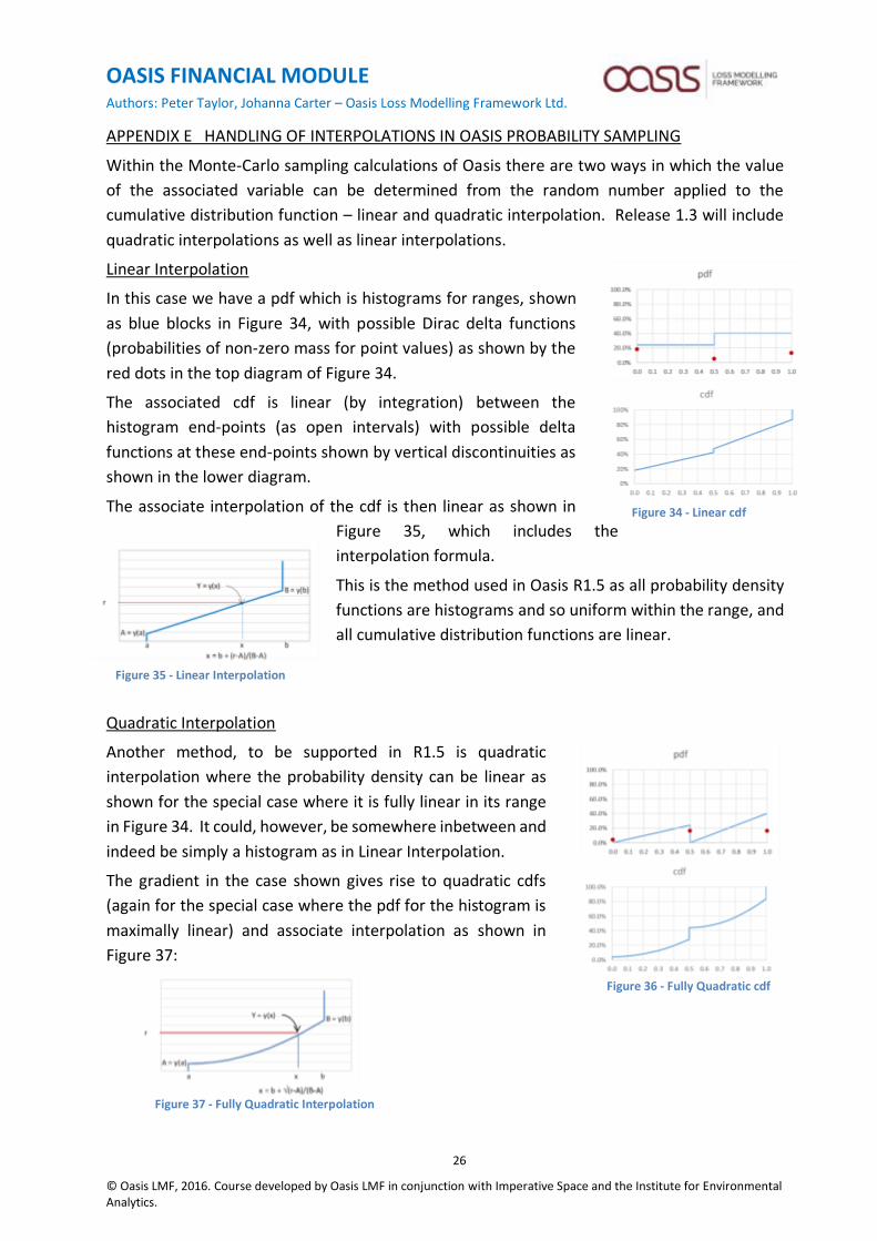
APPENDIX E HANDLING OF INTERPOLATIONS IN OASIS PROBABILITY SAMPLING

Within the Monte-Carlo sampling calculations of Oasis there are two ways in which the value

of the associated variable can be determined from the random number applied to the

cumulative distribution function – linear and quadratic interpolation. Release 1.3 will include

quadratic interpolations as well as linear interpolations.

Linear Interpolation

In this case we have a pdf which is histograms for ranges, shown

as blue blocks in Figure 34, with possible Dirac delta functions

(probabilities of non-zero mass for point values) as shown by the

red dots in the top diagram of Figure 34.

The associated cdf is linear (by integration) between the

histogram end-points (as open intervals) with possible delta

functions at these end-points shown by vertical discontinuities as

shown in the lower diagram.

The associate interpolation of the cdf is then linear as shown in

Figure 35, which includes the

interpolation formula.

This is the method used in Oasis R1.5 as all probability density

functions are histograms and so uniform within the range, and

all cumulative distribution functions are linear.

Quadratic Interpolation

Another method, to be supported in R1.5 is quadratic

interpolation where the probability density can be linear as

shown for the special case where it is fully linear in its range

in Figure 34. It could, however, be somewhere inbetween and

indeed be simply a histogram as in Linear Interpolation.

The gradient in the case shown gives rise to quadratic cdfs

(again for the special case where the pdf for the histogram is

maximally linear) and associate interpolation as shown in

Figure 37:

Figure 34 - Linear cdf

Figure 35 - Linear Interpolation

Figure 36 - Fully Quadratic cdf

Figure 37 - Fully Quadratic Interpolation



27

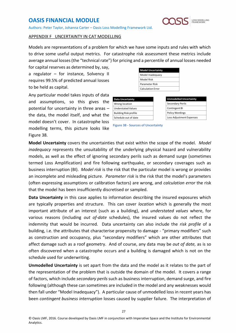
APPENDIX F UNCERTAINTY IN CAT MODELLING

Models are representations of a problem for which we have some inputs and rules with which

to drive some useful output metrics. For catastrophe risk assessment these metrics include

average annual losses (the “technical rate”) for pricing and a percentile of annual losses needed

for capital reserves as determined by, say,

a regulator – for instance, Solvency II

requires 99.5% of predicted annual losses

to be held as capital.

Any particular model takes inputs of data

and assumptions, so this gives the

potential for uncertainty in three areas –

the data, the model itself, and what the

model doesn’t cover. In catastrophe loss

modelling terms, this picture looks like

Figure 38.

Model Uncertainty covers the uncertainties that exist within the scope of the model. Model

inadequacy represents the unsuitability of the underlying physical hazard and vulnerability

models, as well as the effect of ignoring secondary perils such as demand surge (sometimes

termed Loss Amplification) and fire following earthquake, or secondary coverages such as

business interruption (BI). Model risk is the risk that the particular model is wrong or provides

an incomplete and misleading picture. Parameter risk is the risk that the model’s parameters

(often expressing assumptions or calibration factors) are wrong, and calculation error the risk

that the model has been insufficiently discretised or sampled.

Data Uncertainty in this case applies to information describing the insured exposures which

are typically properties and structure. This can cover location which is generally the most

important attribute of an interest (such as a building), and understated values where, for

various reasons (including out of-date schedules), the insured values do not reflect the

indemnity that would be incurred. Data uncertainty can also include the risk profile of a

building, i.e. the attributes that characterise propensity to damage - “primary modifiers” such

as construction and occupancy, plus “secondary modifiers” which are other attributes that

affect damage such as a roof geometry. And of course, any data may be out of date, as is so

often discovered when a catastrophe occurs and a building is damaged which is not on the

schedule used for underwriting.

Unmodelled Uncertainty is set apart from the data and the model as it relates to the part of

the representation of the problem that is outside the domain of the model. It covers a range

of factors, which include secondary perils such as business interruption, demand surge, and fire

following (although these can sometimes are included in the model and any weaknesses would

then fall under “Model Inadequacy”). A particular cause of unmodelled loss in recent years has

been contingent business interruption losses caused by supplier failure. The interpretation of

Figure 38 - Sources of Uncertainty



28

policy wordings by the relevant jurisdiction can also materially affect losses, and a component

of insurance cost generally ignored by modellers is the expenses and fees from adjusters and

lawyers and other third parties involved in a claim, termed loss adjustment expenses. In some

cases these can be a material overhead on top of the pure indemnity cost.

All of these factors go into the risk assessment process and contribute to cost and cost

uncertainty, so it is worth checking how many of the uncertainty factors get addressed when

looking at a particular model.

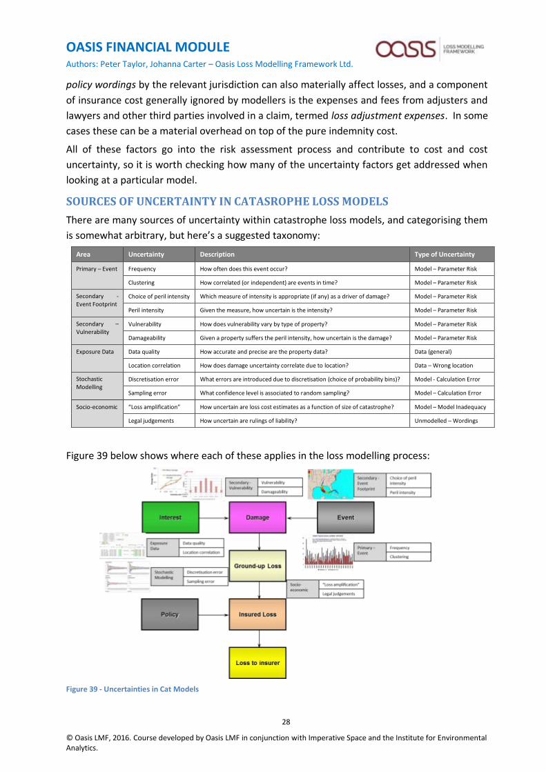
SOURCES OF UNCERTAINTY IN CATASROPHE LOSS MODELS

There are many sources of uncertainty within catastrophe loss models, and categorising them

is somewhat arbitrary, but here’s a suggested taxonomy:

Area Uncertainty Description Type of Uncertainty

Primary – Event Frequency How often does this event occur? Model – Parameter Risk

Clustering How correlated (or independent) are events in time? Model – Parameter Risk

Secondary -

Event Footprint Choice of peril intensity Which measure of intensity is appropriate (if any) as a driver of damage? Model – Parameter Risk

Peril intensity Given the measure, how uncertain is the intensity? Model – Parameter Risk

Secondary – Vulnerability

Vulnerability How does vulnerability vary by type of property? Model – Parameter Risk

Damageability Given a property suffers the peril intensity, how uncertain is the damage? Model – Parameter Risk

Exposure Data Data quality How accurate and precise are the property data? Data (general)

Location correlation How does damage uncertainty correlate due to location? Data – Wrong location

Stochastic Modelling

Discretisation error What errors are introduced due to discretisation (choice of probability bins)? Model - Calculation Error

Sampling error What confidence level is associated to random sampling? Model – Calculation Error

Socio-economic “Loss amplification” How uncertain are loss cost estimates as a function of size of catastrophe? Model – Model Inadequacy

Legal judgements How uncertain are rulings of liability? Unmodelled – Wordings

Figure 39 below shows where each of these applies in the loss modelling process:

Figure 39 - Uncertainties in Cat Models



29

What is then particularly interesting is that many sources of uncertainty lie outside the model

as shown in Figure 40:

Figure 40 - Key Uncertainties outside the Model

The principal concerns are model risk and the unmodelled uncertainties. Model risk is a

problem to which solutions are being developed, and is covered in the next section.

Unmodelled uncertainties need to be allowed for with judgement and subjective allowances,

and some may in due course be brought under the modelled umbrella.

The problem common to all modelling, though, is the quality of the source data. “Garbage In

Garbage Out” data uncertainties are crucial, though they do depend on the model. For

instance, for an aggregate model at US County level using occupancy and high-level

construction type, it is hardly necessary to know the longitude/latitude or the roof geometry as

the model is insensitive to these attributes of a property. Arguably the issue with data is the

sensitivity of the model output to the granularity (precision) and accuracy of the data. We

currently lack methodologies to deal with these uncertainties.



30

APPENDIX G REFERENCES

The following were referenced in this document:

• Sampling Strategies and Convergence = OasisSamplingStrategiesAndConvergence_v1.

• Sub-models = OasisSubModelsR1.5.

• Data Interfaces specification = OasisDataInterfacesR1.5.

• Output specification = OasisOutputsR1.5.

Documents

OASIS FINANCIAL MODULE - dhvptdf78rzwk.cloudfront.net · OASIS FINANCIAL MODULE Authors: Peter Taylor, Johanna Carter – Oasis Loss Modelling Framework Ltd