Embed Size (px)
Citation preview

OAR Lib:
An Open Source Arc Routing Library
Oliver Lum
Department of Applied Mathematics and Scientific Computation(AMSC), University of Maryland
Bruce Golden
Robert H. Smith School of Business, University of [email protected]
September 2013
Abstract
We seek to provide an efficient java implementation of solvers to someof the most ubiquitous problems in the field of Arc Routing, (The ChinesePostman Problem on undirected, directed, mixed, and windy graphs, aswell as the Rural Postman Problem on directed graphs). The projectis open source, and the code will be hosted at https://github.com/
Olibear/ArcRoutingLibrary.
1 Introduction
Broadly speaking, in the realm of vehicle routing, there are two classes of prob-lems; node-routing problems, and arc-routing problems. In the former, the goalis to visit some (sub)set of nodes in a graph while minimizing some cost (ormaximizing some reward) function. Likewise, in the latter, we seek to optimizesome objective function, but this time the requirement is that a (sub)set of edgesgets traversed. For example, the well-known Traveling Salesperson Problem is anode-routing problem that requires the construction of a cycle of minimal costthat visits every node in the graph, (with costs associated with the traversalof each edge). Meanwhile, the analogous problem in arc-routing is the ChinesePostman Problem (CPP), where a candidate cycle must traverse every edge inthe graph.
Unfortunately, the vast majority of outstanding network optimization prob-lems have been shown to be outside of P, (the class of provably polynomial-time
1

solvable problems), which means that it is unlikely that they can be solved tooptimality in a computationally tractable manner. Still, since such problemsare nearly ubiquitous in industry, (with transportation / infrastructure net-works, server topologies, and social networks all benefitting from advances inthe field), there exists a vast literature devoted primarily to devising efficient(meta)heuristics that aim to get close to the optimum without prohibitive com-putational effort. The virtues of a particular heuristic are usually presented viaan analysis of two factors: speed, and proximity to optimality. Of course, inorder to make meaningful comparisons, researchers typically present and solvebenchmark instances that showcase their algorithm’s performance relative tothat of an established alternative.
However, there is another element of variability that is less frequently ac-counted for. Namely, differences in implementation of the same algorithm canbe responsible for discrepancies in results. Given that many of these heuristicsproceed by transforming the more complicated problem into an instance of aneasier problem, (and solving this simpler one to optimality using a known algo-rithm), it is especially important to have standardization with respect to theseeasier problems so that performance can be attributed solely to the merits ofthe heuristics themselves.
2 Approach
To that end, we seek to create an open source code library that provides exactlysuch functionality. More specifically, this library will feature solvers for thefollowing problems: the CPP on a directed graph (DCPP), the CPP on anundirected graph (UCPP), the CPP on a mixed graph (MCPP), the CPP on anundirected graph with directionally asymmetric costs (WPP for Windy PostmanProblem), and the Rural Postman Problem on a directed graph (where not allarcs are required to be traversed in the solution). For each of these problems, ifit is not possible to efficiently solve it to optimality then we present two solvers;one of the more well-known heuristics, and one that is closer to the state-of-the-art. Obviously, if a problem is solvable in polynomial time, we shall implementthe exact algorithm precisely. For the details of each specific algorithm beyondwhat follows, consult references [1] for the Directed CPP, [2] for the UndirectedCPP, [3] and [4] for the Mixed CPP, [5] for the WPP, and [6] and [7] for theDirected RPP.
2.1 Definitions
A graph G is defined as a double (V,L) where V is a set of vertices (alsoreferred to here as nodes), and L a multiset of links. Typically, vertices areindexed naively (i.e. 1,2,3, etc.) while a link is represented as an ordered pair(i, j) where both i and j are members of the vertex set, (we shall not considerhypergraphs here). We call a link an edge if it is undirected (that is, it can betraversed from i to j, and from j to i). A link is called an arc if it is directed
2

(i.e. it can only be traversed from i to j). In the case of arcs, the first elementof the ordered pair is referred to as the tail, while the second is referred to asthe head. For clarity’s sake, an undirected graph is one in which all elements ofthe link set are undirected, and is usually represented as (V,E). Accordingly,a directed graph has only arcs (and is represented (V,A). We call a graphmixed if it is allowed to have links of both types, and use the representation(V,E,A). Finally, we refer to a graph as being windy if it is undirected, andhas asymmetric traversal costs, (i.e. the cost of going from vertex i to vertex j6= the cost of going from vertex j to vertex i).
A graph has the property of being strongly connected if it’s possible to reachany vertex from any other vertex, (more precisely, for any pair of vertices i and j,it is possible to construct an ordered list of links (i0, j0), (j0, j1), (j1, j2)...(jk−1.jk)where i0 = i and jk = j that constructs a valid path from vertex i to vertex j).
A graph is called Eulerian if and only if there exists an Eulerian cycle (apath through the graph that traverses every link in the graph exactly once andreturns to its starting vertex). The various criteria for being Eulerian are asfollows:
• Undirected : A undirected graph is Eulerian ⇐⇒ every node has evendegree.
• Directed : A directed graph is Eulerian ⇐⇒ every node has in-degree =out-degree (a property known as symmetry).
• Mixed : A mixed graph is Eulerian ⇐⇒ every node has even degree, andthe graph is balanced, (for any subset S of V , |number of arcs from S toV \ S - number of arcs from V \ S to S| ≤ number of edges from S toV \S). A sufficient condition to be Eulerian for a mixed graph is for everynode to have even degree, and in-degree = out-degree.
We call a graph G2 = (V2, L2) an augmentation of the graph G1 = (V1, L1)if V1 ⊆ V2, L1 ⊆ L2, and ∀l2ij ∈ L2, (∃l1ij ∈ L1 & cost(l2ij) = cost(l1ij)).Colloquially, this means that every link in the original graph appears in theaugmentation, and that the augmentation only includes copies of links in theoriginal graph.
Finally, we introduce, and distinguish between several notions of degree ofa vertex. In an undirected graph, the degree of a vertex is simply the numberof edges incident on the vertex. In a directed graph, the in-degree of a vertexv is the number of arcs a ∈ A for which v is the head, and the out-degree of avertex v is the number of arcs for which v is the tail. Lastly, for a mixed graph,our definition of in-degree and out-degree remains the same, (i.e. it only takesinto account arcs in the graph), while our definition of degree incorporates bothedges and arcs, (i.e. pretend as though all arcs were undirected).
The problems we intend to solve all fall under the following two categories:
• The Chinese Postman Problem: Given a graph G (either directed, undi-rected, or mixed) and a set of costs cij (associated with traversing the link
3

(i, j)), the task is to find a closed path that traverses each link (edge orarc) at least once and minimizes the total traversal cost. This problem issolved in two steps: the first step (and the most computationally involved)is finding an Eulerian augmentation of the original graph; the second stepis finding the Eulerian cycle in this augmented graph. The second stepcan be performed easily and efficiently in polynomial time (Hierholzer’salgorithm).
• The Rural Postman Problem: Given a graph G = (V,A) (in our case,directed), a set of required arcs AR ⊆ A, and a set of costs cij (associ-ated with traversing the arc (i, j)), the task is to find a closed path thattraverses each required arc at least once and minimizes the total traversalcost. This problem is solved in two steps: the first step is finding an Eu-lerian augmentation of the original graph; the second step is finding theEulerian cycle in this augmented graph. The second step can be performedeasily and efficiently in polynomial time (Hierholzer’s algorithm).
Other common notation includes:
• δ(v) = out-degree − in-degree
• D+ and D− are the set of vertices with δ(v) > 0 and δ(v) < 0.
• Z0+ is the set of non-negative integers, (N).
2.2 Common Algorithms
In the course of developing the library, certain graph algorithms are fairly preva-lent and useful to have split off and available for all solvers / users of the libraryto have access to. Currently, these include:
• Floyd-Warshall All-Pairs Shortest Paths Algorithm
• Dijkstra’s Single-Source Shortest Paths Algorithm with Priority QueueImplementation
• Min-Cost Flow Algorithms (Cycle-Cancelling, and Successive-Shortest Pathsnow implemented).
We detail these algorithms in the following section.
2.2.1 The Cycle-Cancelling Min Cost Flow Algorithm
In order to obtain a minimum cost solution to the flow problem, we have sev-eral options. Currently, we have included both a cycle-cancelling algorithm, aswell as a successive shortest paths algorithm. It is worth noting that our SSPimplementation significantly outperforms our cycle-cancelling implementation,so while we shall review the algorithmic details of both here, only the latter iscurrently called by our solvers.
4

The cycle-cancelling algorithm proceeds by forming residual graphs, detect-ing the presence of negative cycles, and cancelling said cycles by pushing flowaround them. Before we may form the residual graph, though, we must firstfind a feasible solution to the flow problem, (that is, find any acceptable flowthat satisfies the demands, irrespective of cost). Since the flow problem is usu-ally formulated on capacitated graphs (where edges or arcs can only supporta finite amount of traffic), the well-known algorithms all take this into consid-eration (Ford-Fulkerson is the classical algorithm for solving the min cost flowproblem). However, in all of these problems, we are working with uncapaci-tated graphs, and so we may greedily construct a feasible path in the followingmanner:
• Select any node with excess in-degree, call it u.
• Select any node with excess out-degree, call it v.
• Add min |δ(u)|, |δ(v)| shortest paths from u to v.
Assuming we have shortest paths (which we shall explain how to find later),if we simply repeat this procedure until all nodes are symmetric, then we shallhave constructed a feasible solution to the flow problem.
Now, we must introduce the notion of a residual graph. Given a graph G,and a feasible solution X to a flow problem, we may construct its residual graphGX as follows:
• Every vertex in G is also a vertex of GX .
• For each arc (i, j) with capacity rij and cost cij in the original graph G,add two arcs to GX : one arc (i, j) with capacity rij−fij and cost cij , andone arc (j, i) with capacity fij and cost −cij . Here, fij is the amount offlow pushed along the original arc in X.
Now, once we have the residual graph, we simply compute shortest pathsfrom a vertex to itself. If this value is negative, we know a negative cycleexists. We then cancel this cycle by pushing as much flow as possible in theopposite direction (this is trivial to find; it is simply the minimum capacityalong the cycle). Once no more negative cycles exist, the algorithm terminates,and the directed graph we are left with represents a least cost solution to theflow problem.
2.2.2 The Successive Shortest Paths Algorithm
The Successive Shortest Paths Algorithm proceeds by converting the probleminto a single-source, single-sink flow problem, and then repeatedly pushing flowalong the shortest possible path from the source to the sink. In order to performthis conversion, a single source vertex, and a single sink vertex is added to thenetwork. Then, for each vertex vs with supply, a zero-cost arc is added from thesource vertex to vs. This arc has capacity equal to the supply of vs. Similarly,
5
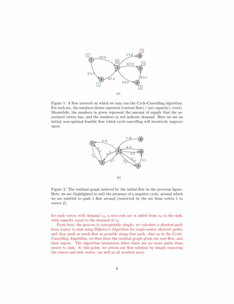
Figure 1: A flow network on which we may run the Cycle-Cancelling algorithm.For each arc, the numbers shown represent (current flow) / (arc capacity), (cost).Meanwhile, the numbers in green represent the amount of supply that the as-sociated vertex has, and the numbers in red indicate demand. Here we see aninitial, non-optimal feasible flow which cycle-cancelling will iteratively improveupon.
Figure 2: The residual graph induced by the initial flow in the previous figure.Here, we see (highlighted in red) the presence of a negative cycle, around whichwe are entitled to push 1 flow around (restricted by the arc from vertex 1 tovertex 2).
for each vertex with demand vd, a zero-cost arc is added from vd to the sink,with capacity equal to the demand of vd.
From here, the process is conceptually simple; we calculate a shortest pathfrom source to sink using Dijkstra’s Algorithm for single-source shortest paths,and then push as much flow as possible along that path. Just as in the Cycle-Cancelling Algorithm, we then form the residual graph given our new flow, andthen repeat. The algorithm terminates when there are no more paths fromsource to sink. At this point, we obtain our flow solution by simply removingthe source and sink vertex, (as well as all incident arcs).
6

Figure 3: The resulting residual graph after 1 flow has been pushed around thenegataive cycle in the previous figure.
The only complication that remains is to resolve a complication that arises tolimitations with Dijkstra’s Algorithm; namely, it’s inability to deal with negativeedge costs. Obviously, negative edge costs arise frequently in residual graphs, sothis concern is non-trivial. However, we avoid having negative costs by reducingthe arc costs at each iteration of the method in the following manner. Consideran arc aij , with original cost cij . Then we set its cost to cij + dist(j)− dist(i)where dist(j) is the shortest path distance from the source to vertex j.
Since we have to repeatedly call Dijkstra’s Algorithm at worst on the orderof O(nB) times, where B is an upper bound on the supply of any node, thenwe can guarantee a complexity of O(n2B log n+ nmB)
Figure 4: A flow network on which we may run the Successive Shortest Pathsalgorithm.
2.2.3 The Floyd-Warshall All-Pairs Shortest Paths Algorithm
There are variety of algorithms to calculate shortest paths, but because of ourchoice of supporting algorithms (particularly the min cost flow algorithm), theFloyd-Warshall algorithm (with path reconstruction) will be one of the idealones to implement.
7

Figure 5: The modified flow network, where each vertex in the original flownetwork that had positive supply has been connected to a new source vertex,and each vertex in the original flow network that had positive demand has beenconnected to the new sink vertex. These added connections all have zero cost,and capacity equal to the supply/demand of the node in the original graph, (e.g.the connection to vertex 1 has capacity 5).
The Floyd-Warshall algorithm proceeds very simply; we construct two |V |×|V | matrices. The first matrix D, will store shortest path distances, where dijwill represent the shortest path cost of getting from vertex i to vertex j. Thesecond matrix P will store information about exactly what the path is; pij willhold the next node in the shortest path from node i to node j.
initially, diagonal elements of D are set to 0, and for each edge (i.j) in thegraph, dij is set to cij , (we are assuming this is not a multigraph; otherwise,we take the cheaper of the two). Every other entry in D is set to infinity (somearbitrarily high number that is greater than the sum of the edge costs), whileevery entry in P is set to some dummy value, (−1 will suffice). Finally, weiterate through all vertex triples (i, j, k), and ask whether the dik + dkj < dij .If so, the new, cheaper cost is stored in dij , and pij gets set to k to signify that,in the shortest path from node i to node j, the next node in the walk is k.
Since all we are doing is traversing ordered triples (i, j, k) where each isallowed to be any number from 1 to n, then clearly the asymptotic complexityis O(n3).
2.2.4 Dijkstra’s Single-Source Shortest Paths Algorithm
Similarly to the Floyd-Warshall All-Pairs Shortest Paths Algorithm, Dijkstra’salgorithm proceeds by maintaining an array of distances and path informationthat we update by examining links in the graph. However, since we are only con-cerned with a single vertex as the starting point, this cuts down the complexityof the problem by a factor of roughly n.
More precisely, the algorithm begins by initializing all distances to infinity,and then examining each of the neighbors of the starting vertex, and assigningthem distances equal to the cost of the edge between them and the startingvertex. Each of these neighbors is then added to a list which contains verticesleft to be examined. The algorithm proceeds by choosing the vertex in the list
8

with the cheapest distance associated with it, and then repeats the process ofexamining its neighbors and updating the distance and path arrays. Each ofthese neighbors is added to our list, and when we have finished examining all ofa vertex’s neighbors, it is ejected from our list. The algorithm terminates whenall vertices have been exhausted.
Since the algorithm considers each edge once, and adds vertices to a priorityqueue that requiresO(n log n), then we have that the algorithm isO(m+n log n).
Figure 6: An intermediate step of Dijkstra’s Algorithm, where vertex 1 is thesource vertex, and we have already assigned distances to nodes 2, 3, and 6. Oncewe have examined all of 1’s neighbors, we then choose the vertex with the leastdistance from the source (that hasn’t yet been interrogated), and repeat theprocess. In this case, 2 was selected as the next node for interrogation, and thealgorithm is currently considering whether or not going from source → vertex2 → vertex 3 beats the previously recorded best distance of 9. It does not, sovertex 3 will retain its distance of 9.
2.3 The Directed Chinese Postman Problem
In light of the notion of an Eulerian graph, (as will be the strategy in general),it suffices to find a least-cost way of augmenting the original graph in order tomake it Eulerian. Obviously, on the augmented graph, the Euler cycle (thatis guaranteed to exist) is an optimal solution to the CPP. With this in mind,we formulate the problem as an integer program that attempts to minimize thecost of the arcs we are adding.
9
Problem Statement:
minimize∑
i or j∈{D+∪D−}
cijxij
subject to: ∑j∈D+
xij = −δ(i), ∀i ∈ D− (1)
∑i∈D−
xij = δ(j), ∀j ∈ D+ (2)
xij ∈ Z0+ (3)
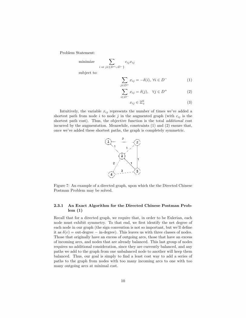
Intuitively, the variable xij represents the number of times we’ve added ashortest path from node i to node j in the augmented graph (with cij is theshortest path cost). Thus, the objective function is the total additional costincurred by the augmentation. Meanwhile, constraints (1) and (2) ensure that,once we’ve added these shortest paths, the graph is completely symmetric.
Figure 7: An example of a directed graph, upon which the the Directed ChinesePostman Problem may be solved.
2.3.1 An Exact Algorithm for the Directed Chinese Postman Prob-lem (1)
Recall that for a directed graph, we require that, in order to be Eulerian, eachnode must exhibit symmetry. To that end, we first identify the net degree ofeach node in our graph (the sign convention is not so important, but we’ll defineit as δ(v) = out-degree − in-degree). This leaves us with three classes of nodes.Those that originally have an excess of outgoing arcs, those that have an excessof incoming arcs, and nodes that are already balanced. This last group of nodesrequires no additional consideration, since they are currently balanced, and anypaths we add to the graph from one unbalanced node to another will keep thembalanced. Thus, our goal is simply to find a least cost way to add a series ofpaths to the graph from nodes with too many incoming arcs to one with toomany outgoing arcs at minimal cost.
10
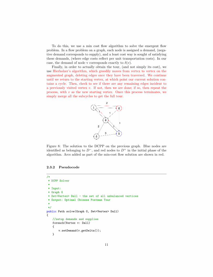
To do this, we use a min cost flow algorithm to solve the emergent flowproblem. In a flow problem on a graph, each node is assigned a demand, (nega-tive demand corresponds to supply), and a least cost way is sought of satisfyingthese demands, (where edge costs reflect per unit transportation costs). In ourcase, the demand of node v corresponds exactly to δ(v).
Finally, in order to actually obtain the tour, (and not simply its cost), weuse Hierholzer’s algorithm, which greedily moves from vertex to vertex on theaugmented graph, deleting edges once they have been traversed. We continueuntil we return to the starting vertex, at which point our current solution con-tains a cycle. Then, check to see if there are any remaining edges incident toa previously visited vertex v. If not, then we are done; if so, then repeat theprocess, with v as the new starting vertex. Once this process terminates, wesimply merge all the subcycles to get the full tour.
Figure 8: The solution to the DCPP on the previous graph. Blue nodes areidentified as belonging to D−, and red nodes to D+ in the initial phase of thealgorithm. Arcs added as part of the min-cost flow solution are shown in red.
2.3.2 Pseudocode
/*
* DCPP Solver
*
* Input:
* Graph G
* Set<Vertex> Dall - the set of all unbalanced vertices
* Output: Optimal Chinese Postman Tour
*
*/
public Path solve(Graph G, Set<Vertex> Dall)
{
//setup demands and supplies
foreach(Vertex v: Dall)
{
v.setDemand(v.getDelta());
}
11

//solve min cost flow
ArrayList<Path> flowSolution = SSPminCostFlow(G);
//add the flow solution
foreach (Path p: flowSolution)
{
G.add(p);
}
return Hierholzers(G);
}
2.4 The Undirected Chinese Postman Problem
Problem Statement:
minimize∑
(i,j)∈E
cijxij
subject to: ∑(i,j)∈Ev
(xij + 1) ≡ 0 mod 2,∀v ∈ V (4)
xij ∈ Z0+ (5)
Here, xij represents the number of additional copies of edge (i, j) in ouraugmented graph. As before, we wish to minimize the added cost, while ensuringevenness of the augmented graph, (constraints (1) and (2) achieve this).
Figure 9: An example of a undirected graph, upon which the the UndirectedChinese Postman Problem may be solved.
2.4.1 An Exact Algorithm For The Undirected Chinese PostmanProblem (2)
The algorithm for the Undirected Chinese Postman Problem is extremely similarto that for the directed variant. We know that an Euler Tour must exist on anundirected graph if every node has even degree, (intuitively, every time we enter
12

a node, we may exit it using a new edge). Thus, the only thing that changeshere is that, rather than worrying about in-degree and out-degree, we simplyseek to pair nodes of odd degree together in a least cost way (so rather thansolving a more complex flow problem, we may solve a min cost perfect matchingproblem). It suffices to identify all of the odd-degree nodes, and carry out amatching algorithm on those (trivially, there will be an even number of them,so parity is not a concern) to solve the undirected Chinese Postman Problem.
Figure 10: The solution to the UCPP on the previous graph. Red nodes areidentified as odd in the initial phase of the algorithm. Edges added as part ofthe matching solution are shown in red.
2.4.2 Pseudocode
/*
* UCPP Solver
*
* Input: Graph G
* Output: Optimal Chinese Postman Tour
*
*/
public Path solve(Graph G)
{
//form odd
Set odd;
foreach(Vertex v: V)
{
if(v.getDelta() % 2 == 1)
{
odd.add(v);
}
}
//compute shortest paths
int[][] shortestPathsMatrix = shortestPaths(odd, G);
//setup matching graph
Graph matchingGraph;
13

foreach(Vertex v1: V)
{
foreach(Vertex v2:V)
{
if(v1 == v2)
continue;
matchingGraph.addEdge(v1, v2, shortestPathsMatrix[v1][v2]);
}
}
//solve min cost matching
ArrayList<Pair> matchSolution = minCostMatching(matchingGraph);
//add the matching solution
foreach (Pair p: matchSolution)
{
G.addShortestPath(p.getFirst(), p.getSecond());
}
return Hierholzers(G);
}
2.5 The Mixed Chinese Postman Problem
Problem Statement:
minimize∑
s∈{A∪E∪E}
csxs
subject to:
y′e + y′e ≥ 1, ∀e ∈ E (6)
xs = y′s + ys, ∀s ∈ A ∪ E ∪ E (7)∑s∈S+
v
xs −∑s∈S−
v
xs = 0, ∀v ∈ V (8)
y′a = 1, ∀a ∈ A (9)
y′e ∈ {0, 1}, ∀e ∈ E ∪ E (10)
ys ∈ Z0+ (11)
First, some notation: y′s is 0 if link s is never traversed, and 1 if it is; ys isthe number of additional times link s is traversed. The set E contains edges ethat are traversed from i to j in the solution, while the set E contains edgese that are traversed from j to i. Thus, xs is the total number of times link sis traversed, and so constraint (1) ensures that each edge is traversed at leastonce, constraint (2) defines xs, constraint (3) ensures symmetry, constraint (4)
14

ensures that arcs are traversed at least once, and constraints (5) and (6) are thebinary constraint for y′s and the integrality constraint for the ys
Figure 11: An example of a mixed graph, upon which the the Mixed ChinesePostman Problem may be solved.
2.5.1 Even-Symmetric-Even (3)
The first heuristic we plan to implement has the same intuitive motivation asthe exact algorithms for the DCPP and UCPP: namely, we try to augment thegraph to reach an Eulerian supergraph in which we know we may locate anEuler tour. In order for a mixed graph to be Eulerian, it must fulfill both of thefollowing properties:
• Evenness: Each node as an even number of incident links.
• Balanced : For each subset of nodes V , the number of undirected arcsbetween V and V \ S must be greater than or equal to the differencebetween the number of arcs from V to V \S and the number of arcs fromV \S to V . (Intuitively, this second condition ensures that we cannot get’stuck’ in a portion of the graph.)
Prima facie, it is difficult to see how one would easily verify the second prop-erty, and so this particular heuristic instead aims to create an even, symmetricgraph, (which, in general, is guaranteed to be balanced).
The Even-Symmetric-Even heuristic has three eponymous phrases; in thefirst, it achieves evenness by carrying out a min-cost matching among the odd-vertices, in the second, it achieves symmetry by using a min-cost flow algorithmon the asymmetric nodes, and in the third, it restores evenness by looking forcycles that may be eliminated safely (because the consist ’mostly’ of links thatwere added in the previous two phases).
1. Phase I, Even: Solve the UCPP on the original graph, treating all arcs asedges. This will produce an augmented graph GE .
2. Phase II, Symmetric: Solve a min cost flow problem on GE , treating eachedge (u, v) as four arcs: the first two (u, v) and (v, u) with cost equal tothe original edge cost and infinite flow capacity; and two (u, v) and (v, u)
15

with zero cost, and flow capacity of 1. If the solution to the flow problemsingularly walks edge (u, v), (that is, in the flow solution, arc (u, v) is onlytraversed once, or arc (v, u) is traversed only once), then we ’orient’ theedge in that direction, otherwise it remains as an edge in our output graphGS .
3. Phase III, Even: Greedily search for cycles that consist of paths betweenany odd-degree nodes left in GS (if there are none, Phase III is unnec-essary). Importantly these paths must alternate between only containingarcs / oriented edges added in Phase II, and only containing edges leftundirected by Phase II. In this way, we ensure that only the parity ofthe odd-degree nodes is changed, while also assigning a direction to allremaining undirected edges. There is a chance that no such cycle exists,and that there are still undirected edges, but the graph will be Eulerianat this point, and so we are done. Once we find one of these alternatingpaths, we orient it (either direction will be equivalent) and duplicate arc-s/oriented edges along the path that follow the orientation, while deletingarcs that are in the opposite direction. Meanwhile, for the sections of thecycle that consist entirely of undirected edges, we simply orient them inthe direction we have chosen to orient the cycle.
Figure 12: The solution to the MCPP on the previous graph. The red arc (2, 5)is added in the initial Even phase, while all other red links are added in theSymmetric phase. The thicker red arrows are to indicate that the edges in theoriginal graph were oriented in the corresponding direction.
2.5.2 Pseudocode
/*
* MCPP Solver
*
* Input: Graph G
* Output: Optimal Chinese Postman Tour
*
*/
public Path solve(Graph G)
16

{
//Phase I: Even
//Solve the UCPP on G, ignoring link direction
Graph G_alt = G;
//make all edges undirected
foreach(Edge e : E_alt)
{
e.setType(Undirected);
}
ArrayList<Path> ucppAugmentation = UCPPAugment(G_alt);
//add the ucpp augmentation
foreach (Path p : ucppAugmentation)
{
G.add(p);
}
//Phase II: Symmetric
//Solve the DCPP on a modified digraph
Graph G_E = G;
//modify the graph to replace edges with four arcs, (two free
and artificial, but with capacity 1).
foreach(Edge e : E_E)
{
if(e.getType() == EDGE.UNDIRECTED)
{
G_E.remove(e);
G_E.add(new Arc(e.getFirst(), e.getSecond(),
e.getCost()));
G_E.add(new Arc(e.getSecond(), e.getFirst(),
e.getCost()));
G_E.add(new Arc(e.getFirst(), e.getSecond(),
0).setCapacity(1));
G_E.add(new Arc(e.getSecond(), e.getFirst(),
0).setCapacity(1));
}
}
//Solve the DCPP on the updated G, breaking edges up into two
arcs
ArrayList<Path> flowSolution = SSPminCostFlow(G_E);
//add the dcpp augmentation, and keep track of whether an edge
gets oriented
foreach (Path p: dcppAugmentation)
{
17

foreach (Arc e: p)
{
if(e.isArtificial())
{
e2 = e.getPartner();
//if we have flow along both artificial arcs,
then leave it undirected
if(p.contains(e2))
{
G.get(e).setType(EDGE.UNORIENTED_PERM);
p.remove(e2);
}
}
//add a copy of the non-artificial arc for each
time it appears in the flow solution
else
{
G.add(e);
}
}
}
//Phase III: Even
Set odd;
foreach (Vertex v : V)
{
if(v.getDegree() % 2 == 1)
{
odd.add(v);
}
}
while(!odd.isEmpty())
{
Vertex vs = odd.getFirst();
Vertex v = vs;
while (odd.contains(v))
{
odd.remove(v);
do
{
//here, added edges is the set of arcs
added in Phase II
addedEdges.remove(<v,w>)
if (<v,w>.getHead() == w )
{
G.add(<v,w>);
}
else
18

G.remove(<w,v>);
v = w;
} while (odd.contains(v))
odd.remove(v);
do
{
//here, unoriented is the set of still
unoriented edges
unoriented.remove((v,w));
G.add(v,w);
v = w;
} while (odd.contains(v) || v == vs)
}
}
return Hierholzers(G);
}
2.5.3 Shortest Additional Path (4)
While most other heuristics for the MCPP do roughly the same thing as Even-Symmetric-Even, (and then sometimes implement an improvement procedureon the generated solution), the Shortest Additional Path Heuristic (SAPH)performs the bulk of its work on a graph that may not even contain a feasibleEuler tour, but manages to ensure that the final output does.
The initial step of SAPH is in fact identical to the second phase of the Even-Symmetric-Even heuristic (where the graph is transformed into a symmetricone). The heuristic then proceeds by exploiting two ideas: first, suppose thatan edge or arc was added to the original graph, and oriented from node A tonode B. Then, if the shortest path cost of going from node A to B is less thanthe cost of traversing this added link, then we ought to replace said link withthe shortest path from A to B.
Figure 13: An example of the first SAPH idea, where we replace an added link(red) with a cheaper shortest path.
19

Second, if an edge was oriented from node A to B, and the two shortestpaths have costs that sum to less than zero, then it’s advantageous to useShortestPath(A → B), (B → A), ShortestPath2(A → B). Although this sec-ond case may seem like a bizarre one to investigate (since the shortest path costswill generally be positive), it is an important one to consider for the SAPH be-cause we may consider a path from A to B as traversing added arcs in theopposite direction (which would correspond to deleting them) and incurring thenegative of its cost.
Figure 14: An example of the second SAPH idea, where we reverse the orienta-tion of an edge and add two ’paths’ from node i to j which sum to a negativecost.
Figure 15: Taken from (4). Edges and arcs in G must end up in one of thefollowing configurations in G∗:
••••••• If an edge remains undirected, it is of type a.
• If an edge gets directed, but not copied, it is of type b.
• If an edge gets directed and copied, but all copies are in the same direction,then it is of type c.
• If an edge gets copied once, and oriented in the opposite direction as theoriginal, it is of type d.
• If an arc is not copied, it is of type e.
• If an arc is copied, it is of type f
20

1. Given a mixed graph G, generate a graph G∗ = (N,M,U) and set ofadded arcs M∗ by solving Phase II of Even-Symmetric-Even on G. Also,generate a graph GM = (N,E+EM , A+AM ) by solving Phase I of Even-Symmetric-Even on G, where EM and AM are the sets of edges and arcsadded from the matching.
2. Choose a random edge/arc in G∗ of type a, c, d or f .
3. Initialize two graphs G1ij = G and G2
ij = G
4. Perform Cost modification 1 on G1ij .
5. Perform Cost modification 2 on G1ij and G2
ij .
6. Apply the first shortest paths idea to the chosen edge/arc.
7. Repeat all steps until there are no more edges of type a, c, d or f .
8. Choose a random edge of type b.
9. Apply the second shortest paths idea to the chosen edge/arc.
10. Go back to Step 8 until there are no more edges of type b.
11. If we were at all able to apply the second shortest paths idea to make anyimprovements, go back to step 1.
12. If there are any more edges (i, j) of type a left in G∗, orient it from i toj, and add a copy (j, i)′ oriented in the opposite direction.
All that remains is to elaborate on exactly what these cost modificationprocedures are, and what their objective is.
Cost modification 1 : This procedure tries to force our shortest paths algo-rithm to traverse links from the matching solution.
1. Given a graph Gij , and GM , and a nonpositive number K, find all edges(f, g) inGij that are also in EM , and, (inGij), set the costs cfg = cgf = K.
2. Locate in Gij , all arcs from AM . If they area of type f (in G∗), then setthe costs cfg = cgf = K. If the arc is of type e, then set cfg = 0, cgf =∞
Cost modification 2 : This procedure tries to force our shortest paths algo-rithm to traverse links that will benefit from our two improvement proceduresat the same time as we examine our chosen link, (which may, for instance, geteliminated as part of a shortest ’path’ from i to j).
1. Given graphs Gij , and G∗, find all edges (f, g) in G∗ that are of type aor d. Also, let c∗fg denote the cost of link (f, g) in the original graph G.Then, set the costs cfg and cgf in Gij to be −c∗fg and −c∗gf .
2. Locate in G∗ all links (f, g) of type c or f , and set the cost cgf in Gij to−c∗fg
3. At whatever point in the process this procedure is being called, set the costof the selected link in Gij to∞ in both directions, (that is cfg = cgf =∞).
21

2.5.4 Pseudocode for SAPH Concepts
/*
* SAPH Concept 1
*
* Input: Graph G1, G2, G_star, link L
* Output: A modified G_star after applying SAPH Concept 1
*
*/
public Graph SAPH1(Graph G1, Graph G2, Link L, Graph G_Star)
{
Graph G_modified = G_Star;
int tempCost = L.getCost();
L.setCost(INFINITY);
Vertex v1 = L.getTail();
Vertex v2 = L.getHead();
Path[][] shortestPathsSolution = shortestPaths(G1);
L.setCost(tempCost); //reset the cost
int cost_ij = 0; //in G2
int cost_ji = 0;
foreach(Link L: shortestPathsSolution[i][j])
{
cost_ij += G2.getCost(L);
}
foreach(Link L: shortestPathsSolution[j][i])
{
cost_ji += G2.getCost(L);
}
if(cost_ij < tempCost && cost_ij < cost_ji)
{
G_modified.add(shortestPathsSolution[i][j]);
}
else if (cost_ji < tempCost && cost_ij > cost_ji)
{
G_modified.add(shortestPathsSolution[j][i]);
}
eliminateCycles(G_modified);
return G_modified;
}
/*
* SAPH Concept 2
*
* Input: Graph G, G_star, Edge e
* Output: A modified G_star after applying SAPH Concept 2
22

*
*/
public Graph SAPH2(Graph G, Edge e, Graph G_Star)
{
Graph G_modified = G_Star;
Graph G_temp = G_Star;
Graph G3 = new Graph(G);
Graph G4 = new Graph(G);
//cheapest path
costModify2(G3, G_Star); //the second cost modification
described later
Path[][] shortestPathsSolution3 = shortestPaths(G3);
G_temp.add(shortestPathsSolution3[i][j]);
//second cheapest path
costModify2(G4, G_modified);
Path[][] shortestPathsSolution4 = shortestPaths(G4);
//if sum of costs is negative, add them to the graph, and remove
the original added edge
if (shortestPathsSolution3[i][j].getCost() +
shortestPathsSolution4[i][j].getCost() < 0)
{
G_modified.add(shortestPathsSolution3[i][j]);
G_modified.add(shortestPathsSolution4[i][j]);
e.reverseOrientation();
}
eliminateCycles(G_modified);
return G_modified;
}
2.6 The Windy Postman Problem
Problem Statement:
23
minimize∑
e+∈E+
ce+xe+ +∑
e−∈E−
ce−xe−
subject to: ∑e+∈E+
xe+ −∑
e−∈E−
xe− = 0, ∀v ∈ V (12)
xe+ + xe− ≥ 1, ∀e ∈ E (13)
xe+ , xe− ∈ Z0+, ∀e ∈ E (14)
As is to be expected, the formulation of the CPP on a windy graph bearsa close resemblance to the formulation of the CPP on an undirected graph.This time, xe+ and xe− represent the number of times an edge e is traversedin the forward direction, and in the reverse direction respectively. With this inmind, constraint (1) enforces symmetry for each vertex (whenever we enter, wemust leave), while constraints (2) and (3) are the usual traversal and integralityrequirements.
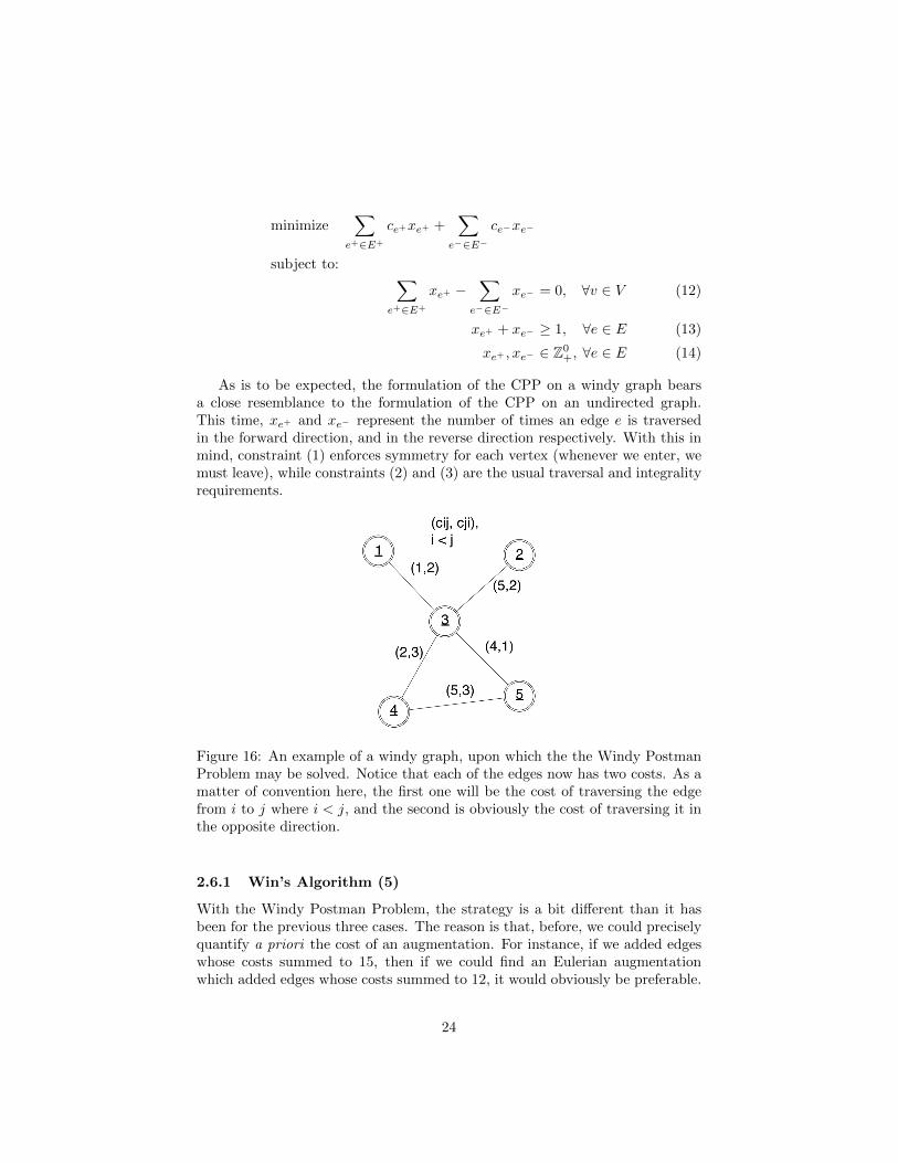
Figure 16: An example of a windy graph, upon which the the Windy PostmanProblem may be solved. Notice that each of the edges now has two costs. As amatter of convention here, the first one will be the cost of traversing the edgefrom i to j where i < j, and the second is obviously the cost of traversing it inthe opposite direction.
2.6.1 Win’s Algorithm (5)
With the Windy Postman Problem, the strategy is a bit different than it hasbeen for the previous three cases. The reason is that, before, we could preciselyquantify a priori the cost of an augmentation. For instance, if we added edgeswhose costs summed to 15, then if we could find an Eulerian augmentationwhich added edges whose costs summed to 12, it would obviously be preferable.
24

Unfortunately, we don’t have that luxury here, since we aren’t sure which di-rection the postman will traverse the edge in his tour, and so the cost of addingan edge is more difficult to assess.
Win’s algorithm attempts to address this difficulty in the simplest way pos-sible: it considers average costs. Thus, is solves the UCPP on the graph GE
which is identical to the input graph G except that it is undirected, with costs
cij =cij + cji
2. Thus produces an Eulerian augmentation to the original graph.
Now, we run a polynomial time algorithm that determines the optimal tour onthis augmented graph:
1. Given the Eulerian graph G, form the digraph DG = (V,A) where thevertex set is identical to that of G, and for each edge in G, if cij < cji,then arc (i, j) is added to A. Otherwise, arc (j, i) is added to A.
2. Create a second digraph D′ = (V,A′) by, for each arc (i, j) ∈ A, adding 3arcs to A′: one arc (i, j) with cost cij and infinite capacity, one arc (j, i)
with cost cji and infinite capacity, and one arc (j, i)′ with costcji − cij
2and capacity 2. This last arc is referred to as being artificial.
3. Solve a min cost flow problem on D′, with demands calculated as they arefor the DCPP on DG.
4. Construct an Eulerian digraph D′′ = (V,A′′) in the following manner. If,in the flow solution, there is 0 flow along the arc (j, i)′, then add 1 + xijcopies of arc (i, j) to A′′. Otherwise, add 1 +xji copies of arc (j, i) to A′′.The Euler cycle on this digraph is an optimal solution to the WPP on G.
Figure 17: The solution to the WPP on the previous graph. The red arcs areadded as part of the flow solution.
25
2.6.2 Pseudocode
/*
* WPP Solver
*
* Input: Graph G
* Output: Approximate solution (path over the G) to the WPP.
*
*/
public Path solve(Graph G)
{
//solve the UCPP on a modified graph that has average costs.
Set E_Undir = new Set();
Graph G_Undir = (V, E_Undir);
//calculate average costs
foreach (Edge e : E)
{
E_Undir.add(new Edge(e.getFirst(), e.getSecond(), (c_ij +
c_ji / 2));
}
//form odd
Set odd;
foreach(Vertex v: V)
{
if(v.getDelta() % 2 == 1)
{
odd.add(v);
}
}
//compute shortest paths
int[][] shortestPathsMatrix = shortestPaths(odd, G);
//solve min cost matching
ArrayList<Path> matchSolution =
minCostMatching(shortestPathsMatrix, odd);
//add the flow solution
foreach (Path p: flowSolution)
{
G.add(p);
}
//Now run Win’s Algorithm to find the optimal WP Cycle on the
Eulerian Graph produced
//by our solution to the UCPP
Set A = new Set();
Set A_prime = new Set();
26

Set A_dprime = new Set();
Graph D_G = (V, A);
Graph D_prime = (V, A_prime);
//Add an arc in the direction of lesser cost for each edge in E
foreach (Vertex e : E)
{
if (c_ij < c_ji)
{
A.add(new Arc(i,j,e.getCost()));
//artificial arc in the high cost direction
A_prime.add(new Arc(j,i,(c_ji - c_ij) /
2).setFlow(2))
}
else
{
A.add(new Arc(j,i,e.getCost()));
//artificla arc in the high cost direction
A_prime.add(new Arc(i,j,(c_ij - c_ji) /
2).setFlow(2))
}
A_prime.add(new Arc(i,j,e.getCost()));
A_prime.add(new Arc(j,i,e.getCost()));
}
ArrayList<Path> minCostSolution = minCostFlow(D_prime);
int[][] flowSolution = new int[][]; //entry is amount of flow
pushed through the arc i,j in the flow solution
int[][] usedArtificial = new int[][]; //entry is 1 if we used
the artificial arc in the flow solution, 0 oth.
foreach(Path p: minCostSolution)
{
foreach(Arc a: p)
{
flowSolution[a.getTail()][a.getHead()] += 1;
//increment the guy in the flow solution matrix
if (a.isArtificial())
usedArtificial[a.getTail()][a.getHead()] =
1;
}
}
for(i=0;i<n;i++)
{
for(j=0;j<n;j++)
{
//If the artificial guy appears in the flow
solution, then add 1 + x copies of the
opposite direction arc
27

if(usedArtificial[i][j] == 1)
{
for(k=0;k<=flowSolution[j][i];k++)
{
A_dprime.add(new Arc(j,i,c_ji));
}
}
else
{
for(k=0;k<=flowSolution[i][j];k++)
{
A_dprime.add)new Arc(i,j,c_ij);
}
}
}
}
Graph G_final = new Graph(V,A_dprime);
return Hierholzers(G_final);
}
2.6.3 Benavent’s H1 (6)
This algorithm is essentially an improvement over Win’s original algorithm inthat it attempts to anticipate the results of the min-cost flow problem earlierin the process. In order to accomplish this, edge costs are modified before thematching is solved (to produce an Eulerian undirected graph):
1. Given the original windy graph G = (V,E), calculate the average edge
cost for the whole graph (Ca =1
2|E|∑
(i,j)∈E cij + cji). Now, consider
edge set E1 = (i, j) ∈ E : {|cij − cji|} > K ∗Ca. Also, define E2 = E\E1.
2. Set up a digraph GdR = (V,A′), where, for each e ∈ E, add 2 arcs in A′,
(i, j) with cost cij and infinite capacity, and (j, i) with cost cji and infinitecapacity. Then, for each e ∈ E1, add an additional artificial arc (j, i) with
costcji − cij
2and capacity 2.
3. Solve a min cost flow problem, with demands given by a reduced graphG′ = (V,A) which contains an arc (i, j) for each edge (i, j) ∈ E1, (herewe assume cij < cji so that the arcs in A are in the direction of cheapertraversal).
4. Compile a list L of edges such that:
• e ∈ E1 and, in the flow solution, there is positive flow across itscorresponding (non-artificial) arcs.
28

• e ∈ E2 and, in the flow solution, there is at least a flow of 2 acrossits corresponding (non-artificial) arcs.
5. For each edge e ∈ L, set its cost to 0 in the original graph, and thencompute the min-cost matching, just as in Win’s algorithm. Then, set allcosts back to what they were in the original graph, and proceed normallyas in Win’s algorithm.
2.6.4 Pseudocode
/*
* WPP Solver2
* H1
*
* Input: Graph G
* Output: Approximate solution (path over the G) to the WPP.
*
*/
public Path solve(Graph G)
{
//compute average traversal cost
int sumCost;
foreach(Edge e: E)
{
sumCost += c_ij + c_ji;
}
double averageCost = sumCost / (2*E.getSize());
double cutOff = .2*averageCost;
//figure out the high disparity edges, and care for them first.
Set E_1, E_2;
foreach(Edge e: E)
{
if (abs(c_ji - c_ij) > cutOff)
{
E_1.add(e);
}
else
E_2.add(e);
}
Set A_prime;
Set A; //holds only arcs in E_1 (cheaper direction of the edge)
Graph G_Rd = (V, A_prime);
foreach(Edge e: E)
{
A_prime.add(new Arc(i,j,c_ij));
A_prime.add(new Arc(j,i,c_ji));
29

if(E_1.contains(e))
{
if(c_ij < c_ji)
{
A_prime.add(new Arc(i,j,c_ij).setFlow(2));
A.add(new Arc(i,j,c_ij);
}
else
{
A_prime.add(new Arc(j,i,c_ji).setFlow(2));
A.add(new Arc(j,i,c_ji);
}
}
}
//use demands from reduced graph
Graph G_E_1 = (V,A);
G_Rd.setDemands(G_E_1);
Set L;
ArrayList<Path> minCostFlowSolution = minCostFlow(G_Rd);
foreach(Path p: minCostFlowSolution)
{
foreach(Edge e: p)
{
if (E_1.contains(e) &&
minCostFlowSolution.contains(a_ij))
L.add(e);
else if(E_2.contains(e) &&
minCostFlowSolution.contains(a_ji))
L.add(e);
}
}
//solve a min cost flow on the reduced cost graph (produced by
solution to flow problem)
Set E_ReducedCost = E;
Graph G_ReducedCost = (V,E_ReducedCost);
foreach(Edge e: E_ReducedCost)
{
if(L.contains(e))
e.setCost(0);
}
ArrayList<Path> minCostMatchingSolution =
minCostMatching(G_ReducedCost);
foreach(Path p: minCostMatchingSolution)
{
G.add(p);
}
30

return WPPSolver(G);
}
2.7 The Directed Rural Postman Problem
Problem Statement:
minimize∑a∈A
caxa
subject to:
xa ≥ 1, ∀a ∈ AR (15)∑{a∈A:hea=i}
xa −∑
{a∈A:taa=i}
xa = 0 , ∀i ∈ V (16)
∑{a∈A:taa∈S 63hea}
xa ≥ 1,∀ ∅ 6= S ⊂ V, |S| ≤ b|V |2c (17)
xa ∈ Z0+ (18)
This IP formulation is a bit more tricky: constraints (1), (2), and (4) shouldlook familiar by now; the first enforces traversal of required arcs, the secondenforces that our path is indeed a cycle, and the fourth demands integrality.However, constraint (3) requires a bit more elaboration. This is a subtourelimination constraint, that prevents a spurious solutions from consideration.For example, suppose a vehicle must service two streets, one in the west endof town, and one in the east. Then, it is unavoidable that this vehicle musttravel the east-west length of town. However, if we did not have constraint (3),it would be considered feasible to have one small cycle in the west part of town,and one in the east, but nothing connecting them. Obviously, this will likely becheaper than any valid route, but this is clearly not admissible as a candidatecircuit.
2.7.1 Christofides’ Algorithm (7)
Broadly speaking, Christofides’ algorithm begins by simplifying the originalgraph (to discard a lot of the unrequired nodes and arcs), and connecting therequired connected components of the graph. It finally solves a min cost flowproblem over the remaining graph to obtain a feasible solution to the DRPP.
1. Given the input graph G = (V,AR ∪ ANR), define the vertex set VR tobe the set of nodes which have at least one required arc incident on them.Then, consider the graph GR = (VR, AR). We form a modified graphG′ = (VR, AR ∪ AS) by making it complete, connecting all vertices in VRwith arcs (i, j) that have cost equal to the shortest path in G between
31

Figure 18: An example of a directed graph, upon which the the Directed RuralPostman Problem may be solved. Green arcs here are required, (i.e. our solutionmust traverse them at least once) while black arcs are not. Also, link costs areomitted for aesthetic reasons.
node i and node j, (these costs are finite because the graph is stronglyconnected). These added arcs comprise the set AS . Now, remove from G′
any arc (i, j) ∈ AS that:
• Has cost cij = cik + ckj for some k ∈ VR.
• Is a duplicate of an arc in AR.
2. Now, starting with the digraph G′, collapse connected required compo-nents into nodes, and solve the minimum spanning arborescence problemon this collapsed graph. Add arcs found in this shortest spanning arbores-cence to a set Tta to indicate that the SSA was rooted in the connectedcomponent ta. Our choice of ta here is arbitrary.
3. Solve a min cost flow on the graph G′ with demands calculated as out −degree− in− degree relative to the arc set AR ∪ Tta , where every arc hasinfinite capacity. Let fij be the amount of flow through arc (i, j) in theflow solution. Then, add fij copies of arc (i, j) to an arc set F . The finalfeasible solution graph is given by GS = (VR, AR ∪ Tta ∪ F ).
It is worth mentioning two improvement procedures which we shall attemptto implement: first, when we constructed the shortest spanning arborescence,we fixed a root node, and so we may repeat the algorithm with k different SSA’s,where k is the number of required components of the simplified graph G′, andchoose the best solution; second, once we have constructed our final augmentedgraph GS , it’s possible that replacing two arcs (i, j) and (j, l) with the singlearc (i, l) (if this is a valid arc) would leave GS still strongly connected, and soreplacing the two arcs with this one would leave us feasible and at least as goodfrom a cost perspective.
2.7.2 Pseudocode
32

Figure 19: The solution to the DRPP on the previous graph. Notice thatnode 7 has disappeared because of our simplification of the graph, however itis important to note that c34 will be increased to c37 + c74, and an analogousalteration will be made for c43.
/*
* DRPP
* Christofides
*
* Input: Graph G
* Output: Approximate solution (path over the G) to the WPP.
*
*/
public Path solve(Graph G)
{
//Set up the required graph
//the required items
Set A_R, V_R;
Graph G_R = (V_R,A_R);
foreach(Arc a: A)
{
if(a.isRequired())
{
A_R.add(a);
V_R.add(a.getTail());
V_R.add(a.getHead());
}
}
//the required strongly connected components
Set<Set<Vertex>> stronglyConnectedComponents =
G_R.getStronglyConnectedComponents();
//make it complete
Path[][] shortestPaths = computeShortestPaths(G,V_R);
for(int i=0;i<V_R.size();i++)
{
for(int j=0;j<=i;j++)
33

{
boolean skip = false;
//don’t add a path if it represents a redundancy
cost = shortestPaths[i][j].getCost();
foreach(Vertex v_k: V_R)
{
if(cost == shortestPaths[i][k].getCost() +
shortestPaths[k][j].getCost())
{
skip = true;
break;
}
}
if(skip)
continue;
//don’t add a copy of a required arc
if(shortestPaths[i][j] == a_ij &&
a_ij.isRequired())
continue;
G_R.add(shortestPaths[i][j]);
}
}
//form a graph on which we solve the minimum spanning
arborescence on
Set V_Collapsed, A_Collapsed;
Graph G_R_Collapsed = G_R.collapse(stronglyConnectedComponents);
Set<Arc> minimumSpanningArborescence = MSA(G_R_Collapsed);
//arc set A_R U minSpanningArborescence
Set A_demands = A_R;
A_demands.addAll(minimumSpanningArborescence);
G_R.setDemands(A_demands);
ArrayList<Path> minCostFLowSolution = minCostFlow(G_R);
foreach(Path p: minCostFLowSolution)
{
G_R.add(p);
}
return Hierholzers(G_final);
}
2.7.3 Benavent’s WRPP1 (8)
Although originally created to deal with the more general Windy Rural PostmanProblem, we may model the DRPP as an instance of the WRPP by assigninginfinite cost to traversing edges in the opposite direction of their corresponding
34

arc. Once we do this, the procedure is identical to Win’s algorithm for the WindyPostman Problem, except that here, before we begin, we compute the connectedcomponents of the graph induced by the required arcs GR, and connect themwith a shortest spanning arborescence. The arcs that are associated with thisSSA are added to the set of required arcs, forming a new required graph G′R onwhich we run Win’s WPP algorithm.
2.7.4 Pseudocode
/*
* DRPP
* Benavent
*
* Input: Graph G
* Output: Approximate solution (path over the G) to the WPP.
*
*/
public Path solve(Graph G)
{
private static final INFINITY = INTEGER.MAX;
//Set up the required graph
//the required items
Set A_R, V_R;
Graph G_R = (V_R,A_R);
foreach(Arc a: A)
{
if(a.isRequired())
{
A_R.add(a);
V_R.add(a.getTail());
V_R.add(a.getHead());
}
}
//the required strongly connected components
Set<Set<Vertex>> stronglyConnectedComponents =
G_R.getStronglyConnectedComponents();
//form a graph on which we solve the minimum spanning
arborescence on
Set V_Collapsed, A_Collapsed;
Graph G_R_Collapsed = G_R.collapse(stronglyConnectedComponents);
Set<Arc> minimumSpanningArborescence = MSA(G_R_Collapsed);
//arc set A_R U minSpanningArborescence
Set A_demands = A_R;
A_demands.addAll(minimumSpanningArborescence);
35

G_R.setDemands(A_demands);
ArrayList<Path> minCostFLowSolution = minCostFlow(G_R);
foreach(Path p: minCostFLowSolution)
{
A_R.add(p);
}
Set E_Windy;
Graph G_W = (V_R, E_Windy);
//Now set up the Windy Graph
foreach(Arc a: A_R)
{
E_Windy.add(new
Edge(a.getTail(),a.getHead(),a.getCost(),INFINITY));
}
return WPP2Solve(G_W);
}
2.8 Results
In the following section, we present computational results for the current con-tents of the library. All tests were performed on a MacBook Air(August 2012),running an i5-3427u processor. Whenever possible, we test on publicly availabletest instances modeled on real street networks, posted at http://www.uv.es/
corberan/instancias.htm. Our library contains a parser for the format pro-vided therein which outputs a graph object that is used as input to our solvers.For the UCPP and DCPP, and the subroutines shown here, we have writtena graph generator that randomly generates a graph given density, number ofvertices, and connectedness (boolean) as inputs.
As mentioned when the details of the algorithm were presented, the Floyd-Warshall All-Pairs Shortest Paths algorithm ought to have an expected asymp-totic complexity of O(n3), and indeed, we can see this borne out by our partic-ular implementation.
Run times for our first attempt at implementing the Successive ShortestPaths Min-Cost Flow algorithm. This algorithm was deemed necessary aftera cycle-cancelling algorithm produced run times that were prohibitively high.Performance increased nearly an order of magnitude, even for graphs of rela-tively small size. Obviously, since the algorithm has super-linear complexity,this improvement is amplified for more complex instances. Still, an analysisof the amount of time spent in each subroutine revealed an algorithmic ineffi-ciency. Namely, an All-Pairs Shortest Paths when calculating the shortest pathalong which to push flow, when a Single-Source Shortest Paths algorithm wouldsuffice (we are always pushing flow from the source to the sink). Thus, oncethis correction was made, and Dijkstra’s algorithm was substituted, we achieved
36

Figure 20: Run times for our implementation of the Floyd-Warshall All-PairsShortest Paths subroutine.
Figure 21: Run times for our implementation of the Successive Shortest PathsMin-Cost Flow subroutine.
much better run times, as illustrated in Figure 17.For the Directed and Undirected Chinese Postman Problems, the majority of
the work involved is simply obtaining the solution to the flow / matching prob-lem induced by the original graph, and so for similar problem complexity, thetwo have comparable performance. It is worth noting that in order to solve themin cost perfect matching problem, we use the publicly available, and extremelyefficient C++ implementation of the Blossom algorithm presented in a paperby Kolmogorov in 2009. To call this code from Java, we write a simple func-tion wrapper, and use the Java Native Interface to communicate cross-platform.
37

Figure 22: Run times for our implementation of the Successive Shortest PathsMin-Cost FLow subroutine (blue), and again after correcting for the algorithmicinefficiency of using an All-Pairs Shortest Paths algorithm where a single-sourceone would suffice.
Figure 23: Run times for our implementation of the Directed Chinese PostmanProblem Exact Solver.
This explains the seemingly sporadic nature of the UCPP Solver’s performanceon smaller problem instances, since in these instances it’s the overhead of callingthe function rather than the function itself that dominates the compute time.
The computational results for Frederickson’s MCPP Heuristic are actuallyquite surprising. Seeing as the heuristic is, at the worst, a 5/3-approximation(meaning we could at worst be 66% away from optimality), one might reasonablyexpect to see solution quality vary over that range, (and indeed, it is theoretically
38

Figure 24: Run times for our implementation of the Undirected Chinese Post-man Problem Exact Solver.
Figure 25: Run times for our implementation of Frederickson’s Mixed ChinesePostman Problem Heuristic.
possible for this to be the case). However, on these instances, modeled after real-world street networks, we see that the solution quality is actually quite good;we never are worse than 3% away from optimality, and are frequently less than1.5% away. Furthermore, the distance from optimality does not appear to growin any predictable way with problem size or complexity, which is encouragingin terms of generalizing these results.
39

Figure 26: An illustration of the solution quality of Frederickson’s MCPPHeuristic.
Figure 27: The percent away from optimality that Frederickson’s MCPP Heuris-tic achieves. As a rule of thumb, the instances grow in complexity as a functionof their instance number.
2.9 Remarks
Furthermore, since we fully intend for this library to be used in circumstancesbeyond the context of our own endeavors, if time permits, we shall attempts toinclude several useful utilities. These include, but are not necessarily limitedto the following: the capability to use existing software to visualize graphscreated using our library (currently Gephi seems to be the 3rd party software ofchoice); the ability to easily exchange problem instances by allowing export tothe prevailing industry standard graphml format; and the option to make calls
40

to CPLEX and Gurobi in solvers.Ultimately, upon completion of this code base, we seek to extend the work
done by Benjamin Dussault et al. on the variant of the Windy Postman Problemwith precedence discussed in [8]. In this work, an additional complication to thestandard WPP is thrown in: an edge has reduced cost upon repeat traversal (ofcourse, the costs are still asymmetric). This is meant to reflect a scenario wheresome impediment to progress is removed during the first traversal, and so anyfurther traversal takes less resources. The paper presents a method of producinga good initial feasible solution, and then details an improvement procedurethat involves permuting cycles found in the original solution. However, thesepermutations are essentially arrived at randomly. We hope to devise a moresystematic way of choosing which permutations tend to yield better solutions,and use this knowledge to refine the local search procedure.
3 Implementation
The library is written in Java, which exposes an interface that allows C++code to be run in the event that performance concerns necessitate that certainportions to be sped up. The code will be hosted, (both during development, andupon completion) as a repository on my personal github at https://github.
com/Olibear/ArcRoutingLibrary.We choose Java for several reasons. First, it appears as though the general
developer industry is moving towards adopting Java as the de facto standard formost modern projects. Second, as has already been mentioned, Java providesways to interface with its main competitor C++, and so concerns over lossof flexibility may be eschewed. Third, libraries in the field of combinatorialoptimization (e.g. LEMON, Boost, etc.) have traditionally been written inC++, and so we hope that ours will help fill the void of Java-based graphlibraries.
Git provides convenient means of synchronizing, sharing, and storing code.Github also tracks accesses to the repository so that we may collect meaningfulmetrics on dissemination of the project.
4 Databases
In order to test the performance and accuracy of our library, we shall run oursolvers on a collection of benchmark instances that have known solutions andare publicly available. For the the directed and undirected Chinese postmanproblem, we shall simply generate our own test instances, (since these algorithmsare old, exact, and polynomial, test instances aren’t prevalent in the literature).Furthermore, we shall do the same for the Directed Rural Postman, since theredo not seem to be public instances available for this particular variant.
The procedure for generating test instances for the DCPP and UCPP willsimply be to randomly generate a graph, (consider all pairs (i, j) and add them
41
to the graph with probability p1, and then connect components of the grapharbitrarily). We generate instances to the DRPP the same way we get instancesto the DCPP, and then just pick a subset of required arcs with probability p2.If time permits, we shall investigate the effect that these have on performance.
For the Mixed and Windy Postman, we shall use the test instances madepublic by Dr. Angel Corberan at his website (http://www.uv.es/corberan/instancias.htm) which have documented solutions available at the same place.
5 Validation
Broadly speaking, there are two types of components to the project that needvalidation: the subroutines, and the solvers themselves (therefore, the high-level algorithm that makes use of the subroutines). For the former, we comparethe output of our implementations to those given in (10). For both the flowalgorithms and the shortest path calculations, we compare only the costs, asthe specific flow / shortest path solutions are liable to be different if multipleexist with the same objective value, but none of the solvers in which thesesubroutines are invoked specify any particular type of tie-breaking mechanismas preferable, so we do not worry about any such discrepancies. All we notehere, is that, for our own implementations, so long as the ordering of the verticesand arcs is the same, we get identical results on consecutive runs.
For the DCPP and UCPP, we simply ensure that we are reaching the optimalsolution, as well as that the run time of the algorithm scales polynomially (justby recording runtime as a function of the problem size of the test instances). Wedo so by making calls to the Gurobi Java API and setting up Integer Programformulations for each of the problems, and then comparing the optimal objectivevalue to our own.
For each of the NP-Hard problems we shall attempts to solve, we attemptto validate our efforts by performing Wilcoxon’s Signed Rank Test. Wilcoxon’sSigned Rank Test proceeds by considering both the distance between pairedobservations, and the sign of the distance. The null hypothesis will be that ourresults are identical to the results provided in the papers in which the heuristicsare proposed. Although our test instances will be different from the instancesused in the paper, a common metric in the literature is to consider percent fromoptimality which is exactly the metric we shall use in order to determine thetest statistic.
6 Testing
In addition to running our heuristics on several more complex benchmark in-stances taken from our data sources, we shall run our solvers on several simple,small-sized instances that are constructed to be solvable to optimality by in-spection, as well as several non-trivial instances that we solve in CPLEX andGurobi to optimality. In this way, we can ensure that the algorithm is executing
42
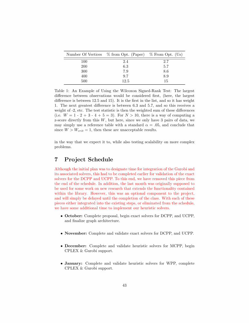
Number Of Vertices % from Opt. (Paper) % From Opt. (Us)
100 2.4 2.7200 6.3 5.7300 7.9 8.6400 9.7 8.9500 12.5 15
Table 1: An Example of Using the Wilcoxon Signed-Rank Test: The largestdifference between observations would be considered first, (here, the largestdifference is between 12.5 and 15). It is the first in the list, and so it has weight1. The next greatest difference is between 6.3 and 5.7, and so this receives aweight of -2, etc. The test statistic is then the weighted sum of these differences(i.e. W = 1 - 2 + 3 - 4 + 5 = 3). For N > 10, there is a way of computing az-score directly from this W , but here, since we only have 3 pairs of data, wemay simply use a reference table with a standard α = .05, and conclude thatsince W > Wcrit = 1, then these are unacceptable results.
in the way that we expect it to, while also testing scalability on more complexproblems.
7 Project Schedule
Although the initial plan was to designate time for integration of the Gurobi andits associated solvers, this had to be completed earlier for validation of the exactsolvers for the DCPP and UCPP. To this end, we have removed this piece fromthe end of the schedule. In addition, the last month was originally supposed tobe used for some work on new research that extends the functionality containedwithin the library. However, this was an optional component to the project,and will simply be delayed until the completion of the class. With each of thesepieces either integrated into the existing steps, or eliminated from the schedule,we have some additional time to implement our heuristic solvers.
• October: Complete proposal, begin exact solvers for DCPP, and UCPP,and finalize graph architecture.
• November: Complete and validate exact solvers for DCPP, and UCPP.
• December: Complete and validate heuristic solvers for MCPP, beginCPLEX & Gurobi support.
• January: Complete and validate heuristic solvers for WPP, completeCPLEX & Gurobi support.
43

• February - March: Complete and validate heuristic solvers for DRPP.
• April: Performance Optimization & Visualization
• May: Final Report
8 Milestones
At the conclusion of each month, solvers that ought to be completed shouldhave test cases ready to benchmark performance, and verify the validity ofthe solutions produced by the library. For instance, by the end of October,(assuming all goes according to plan), we hope to be able to set up a testinstance, run our DCPP or UCPP solver on it, and collect metrics like runtime, solution feasibility, etc.
9 Deliverables
By the conclusion of the year, we hope to have compiled an easily accessible,easily usable, easily extensible library of code designed to solve the aforemen-tioned problems. In addition, if time allows, we also hope to be able to integratebenchmarking and visualization utilities into the library (as opposed to simplycobbled together for our own use). The mid-year and final reports, as well asdocumentation (including a readme, and tutorials/examples) and all of the testinstances (both generated and taken from Corberan) will be available on thecentral github page.
References
[1] Thimbleby, Harold. ”The directed chinese postman problem.” Software:Practice and Experience 33.11 (2003): 1081-1096.
[2] http://www.ise.ncsu.edu/fangroup/or766.dir/or766_ch9.pdf
[3] Frederickson, Greg N. ”Approximation algorithms for some postman prob-lems.” Journal of the ACM (JACM) 26.3 (1979): 538-554.
[4] Yaoyuenyong, Kriangchai, Peerayuth Charnsethikul, and Vira Chankong.”A heuristic algorithm for the mixed Chinese postman problem.” Optimiza-tion and Engineering 3.2 (2002): 157-187.
[5] Win, Zaw. ”On the windy postman problem on Eulerian graphs.” Mathe-matical Programming 44.1-3 (1989): 97-112.
44

[6] Benavent, Enrique, et al. ”New heuristic algorithms for the windy ruralpostman problem.” Computers & operations research 32.12 (2005): 3111-3128.
[7] Eiselt, Horst A., Michel Gendreau, and Gilbert Laporte. ”Arc routing prob-lems, part II: The rural postman problem.” Operations Research 43.3 (1995):399-414.
[8] Campos, V., and J. V. Savall. ”A computational study of several heuristicsfor the DRPP.” Computational Optimization and Applications 4.1 (1995):67-77. (Replace this with Carmine’s paper when I get it).
[9] Dussault, Benjamin, et al. ”Plowing with precedence: A variant of the windypostman problem.” Computers & Operations Research (2012).
[10] Lau, Hang T. A Java library of graph algorithms and optimization. CRCPress, 2010.
[11] Derigs, Ulrich. Optimization and operations research. Eolss PublishersCompany Limited, 2009.
[12] http://en.wikipedia.org/wiki/Dijkstra’s_algorithm
[13] http://community.topcoder.com/tc?module=Static&d1=
tutorials&d2=minimumCostFlow2
45