Embed Size (px)
Citation preview

Off–lattice models of planar aggregation
Vittoria Silvestri

December 7, 2016
Contents
Chapter 1. Complex Analysis preliminaries 5
1. Holomorphic functions and Cauchy integration 5
2. The complex logarithm 7
3. Conformal maps 8
4. Conformal invariance of Brownian motion 10
5. Density of harmonic measure 14
Chapter 2. Hastings–Levitov models 17
1. Discrete aggregation models 17
2. A continuum model: Hastings–Levitov growth 19
Chapter 3. Small particle limit 27
1. Preliminary estimates 30
2. The scaling limit result 34
3. Scaling limit of regularised HL(α) clusters 40
Chapter 4. Fluctuations 43
1. Preliminary estimates 45
2. Pointwise fluctuations 46
3. Global fluctuations 53
Bibliography 61
3


CHAPTER 1
Complex Analysis preliminaries
In this first chapter we recall, for convenience of the reader and to fix the notation,
some basic concepts from Complex Analysis that we will use throughout the course.
1. Holomorphic functions and Cauchy integration
Definition 1.1. A domain in the complex plane C is a non-empty connected set. A
domain D is simply connected if it is path connected and every loop in D is homotopic
to a point. Equivalently, D is simply connected if C ∪ ∞ \D is connected.
Here are some examples.
• D = z ∈ C : |z| < 1 is simply connected.
• H = z ∈ C : Im(z) > 0 is simply connected.
• C ∪ ∞ without a strip is simply connected.
• C ∪ ∞ without an annulus is not simply connected.
Definition 1.2. A function f : C → C is said to be holomorphic (or analytic) in
a domain D iff for all z ∈ D the limit
limh→0
f(z + h)− f(z)
h
exists in C. In this case we define f ′(z) as the value of such limit.
We remark that, identifying C with R2, we see that f is holomorphic iff f is differen-
tiable, and the Cauchy-Riemann (C-R) equations hold:
(C-R)
∂ Re(f)
∂x=∂ Im(f)
∂y∂ Re(f)
∂y= −∂ Im(f)
∂x.
Moreover, if f is holomorphic then Re(f) and Im(f) are real-harmonic functions (the
reader should check this as a straightforward exercise).
1.1. The Cauchy integral theorem. In this section we discuss integration of com-
plex valued functions along piecewise differentiable curves in the complex plane.
Definition 1.3. A curve is a continuous map γ : [a, b] → C, a < b, from a compact
real interval into the complex plane. A curve is closed if it starts and ends at the same
points, i.e. γ(a) = γ(b). A curve is piecewise differentiable if there exists a finite
partition of [a, b] such that in each interval of this partition the function γ is differentiable.
5
6 1. COMPLEX ANALYSIS PRELIMINARIES
For example, a rectangle is a closed curve which is piecewise differentiable but not
differentiable. With a slight abuse of notation, we often write γ in place of γ([a, b]),
regarding it as a closed subset of C. From now on we work with differentiable curves for
simplicity. Everything extends trivially to the piecewise differentiable case.
Definition 1.4 (Contour integral). Let γ be a differentiable curve contained in a
domain D ⊂ C, and let f : D → C be a continuous function. Then the expression∫γf(z)dz :=
∫ b
af(γ(t))γ′(t)dt
is called contour integral of f on γ.
Note that, by the fundamental theorem of calculus, if f had a primitive F on D (i.e.
F is differentiable with F ′ = f) then∫γf(z)dz = F (γ(b))− F (γ(a)).
In particular, the integral of f along any closed curve vanishes. On connected open
domains this condition turns out to be sufficient for the existence of a primitive.
Proposition 1.1 (cf. [Car95], Chapter II). Let D be a connected open domain in C.
Then D is arcwise connected, i.e. for any two points z0, z1 in D there exists a piecewise
differentiable curve from z0 to z1 contained in D. Moreover, if f : D → C is a continuous
function, then the following statements are equivalent:
• f has a primitive on D,
•∫γ f(z)dz = 0 for any closed curve γ contained in D,
• the integral of f along any curve in D depends only on the starting and end points
of the curve.
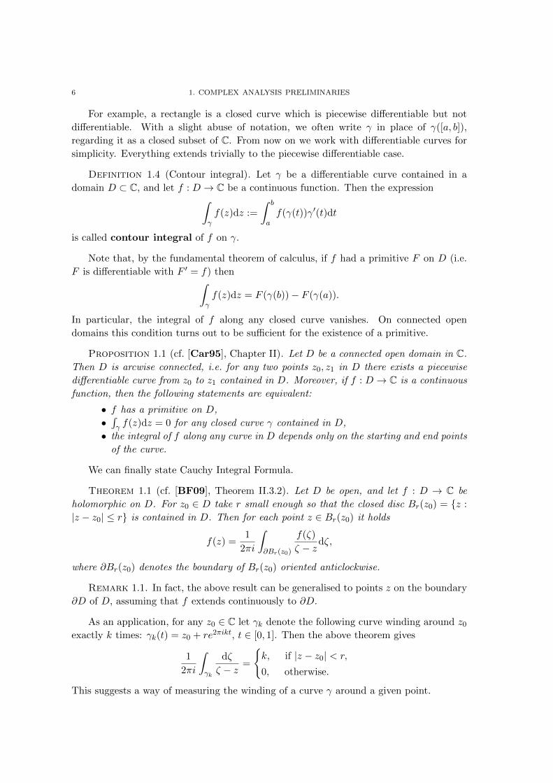
We can finally state Cauchy Integral Formula.
Theorem 1.1 (cf. [BF09], Theorem II.3.2). Let D be open, and let f : D → C be
holomorphic on D. For z0 ∈ D take r small enough so that the closed disc Br(z0) = z :
|z − z0| ≤ r is contained in D. Then for each point z ∈ Br(z0) it holds
f(z) =1
2πi
∫∂Br(z0)
f(ζ)
ζ − zdζ,
where ∂Br(z0) denotes the boundary of Br(z0) oriented anticlockwise.
Remark 1.1. In fact, the above result can be generalised to points z on the boundary
∂D of D, assuming that f extends continuously to ∂D.
As an application, for any z0 ∈ C let γk denote the following curve winding around z0
exactly k times: γk(t) = z0 + re2πikt, t ∈ [0, 1]. Then the above theorem gives
1
2πi
∫γk
dζ
ζ − z =
k, if |z − z0| < r,
0, otherwise.
This suggests a way of measuring the winding of a curve γ around a given point.
2. THE COMPLEX LOGARITHM 7
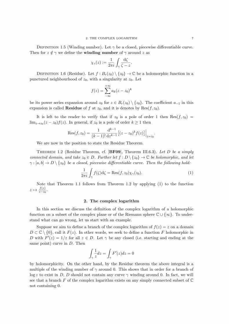
Definition 1.5 (Winding number). Let γ be a closed, piecewise differentiable curve.
Then for z /∈ γ we define the winding number of γ around z as
χγ(z) :=1
2πi
∫γ
dζ
ζ − z .
Definition 1.6 (Residue). Let f : Br(z0) \ z0 → C be a holomorphic function in a
punctured neighbourhood of z0, with a singularity at z0. Let
f(z) =+∞∑−∞
ak(z − z0)k
be its power series expansion around z0 for z ∈ Br(z0) \ z0. The coefficient a−1 in this
expansion is called Residue of f at z0, and it is denotes by Res(f, z0).
It is left to the reader to verify that if z0 is a pole of order 1 then Res(f, z0) =
limz→z0(z − z0)f(z). In general, if z0 is a pole of order k ≥ 1 then
Res(f, z0) =1
(k − 1)!
dk−1
dzk−1
[(z − z0)kf(z)
]∣∣∣z=z0
.
We are now in the position to state the Residue Theorem.
Theorem 1.2 (Residue Theorem, cf. [BF09], Theorem III.6.3). Let D be a simply
connected domain, and take z0 ∈ D. Further let f : D \ z0 → C be holomorphic, and let
γ : [a, b]→ D \ z0 be a closed, piecewise differentiable curve. Then the following hold:
1
2πi
∫γf(ζ)dζ = Res(f, z0)χγ(z0). (1)
Note that Theorem 1.1 follows from Theorem 1.2 by applying (1) to the function
z 7→ f(z)z−z0 .
2. The complex logarithm
In this section we discuss the definition of the complex logarithm of a holomorphic
function on a subset of the complex plane or of the Riemann sphere C ∪ ∞. To under-
stand what can go wrong, let us start with an example.
Suppose we aim to define a branch of the complex logarithm of f(z) = z on a domain
D ⊂ C \ 0, call it F (z). In other words, we seek to define a function F holomorphic in
D with F ′(z) = 1/z for all z ∈ D. Let γ be any closed (i.e. starting and ending at the
same point) curve in D. Then ∫γ
1
zdz =
∫γF ′(z)dz = 0
by holomorphicity. On the other hand, by the Residue theorem the above integral is a
multiple of the winding number of γ around 0. This shows that in order for a branch of
log z to exist in D, D should not contain any curve γ winding around 0. In fact, we will
see that a branch F of the complex logarithm exists on any simply connected subset of Cnot containing 0.
8 1. COMPLEX ANALYSIS PRELIMINARIES
What does it change when working with a subset of C∪∞ rather than of C? When
adding the point at infinity, we simply have to check whether we can allow curves to wind
around ∞. Again, we find∫γ
1
zdz = −2πiRes
(1
z,∞)
= 2πiRes(1
z, 0)
= 2πi,
where we have used that Res(f(z),∞
)= −Res
(1z2 f(
1z
), 0). This shows that the domain
of holomorphicity of F cannot contain any curve with non–trivial winding number around
∞. In order to avoid both curves winding around 0 and curves winding around ∞, one
often chooses to cut the Riemann sphere along the negative real axis.
Now let us look at the definition of a branch of the logarithm of a holomorphic function
f(z) on some simply connected subset D of the Riemann sphere containing the point at
infinity. Note that if f is holomorphic and non-zero in D∩C, then its logarithmic derivative
f ′(z)/f(z) is holomorphic on the same set, and so it has vanishing integral along any closed
curve contained in D ∩ C not winding around the point at infinity. Again, we only need
to check what the addition of the point at infinity entails. Take any closed curve γ in D
winding around ∞. Then∫γ
f ′(z)
f(z)dz = 2πiRes
(f ′(z)f(z)
,∞)
= −2πiRes( 1
z2
f ′(1/z)
f(1/z), 0). (2)
Suppose that our holomorphic function f is such that the far r.h.s. is equal to zero. Then∫γf ′(z)f(z) dz = 0 for any closed curve γ in D ⊂ C ∪ ∞, which implies that f ′(z)/f(z) has
a primitive in D (cf. [Car95], Chapter II). Thus we can set
F (z) = F (z0) +
∫z0→z
f ′(w)
f(w)dw
for arbitrary z0 ∈ D, where z0 → z denotes any curve from z0 to z contained in D, and
F (z0) is defined so that eF (z0) = f(z0) (this fixes the branch). The above definition is well
posed since the integral along any closed curve in D of f ′(z)/f(z) vanishes. We call F a
branch of the logarithm of f in D.
Remark 1.2. In the next chapters we will be interested in defining the logarithm of
the holomorphic functions Φn(z)/z, Γn(z)/z in a subset of the Riemann sphere. For these
functions we have a prescribed normalization at infinity, and the reader can check that
indeed the expressions in in (2) vanish for any curve winding around the point at infinity.
3. Conformal maps
Definition 1.7. A function f is a conformal map in D if it is holomorphic in D
and f ′(z) 6= 0 for all z ∈ D.
Definition 1.8. A function f is a conformal isomorphism it is a bijection in D
and both f and its inverse are conformal in D.
Note that, by definition, every conformal isomorphism is a conformal map. The vice
versa is not true: as a counterexample one can take the complex exponential (confor-
mal, but not injective). On the other hand, locally every conformal map is a conformal
isomorphism.
3. CONFORMAL MAPS 9
Definition 1.9 (Moebius transformations). A Moebius transformation is any function
f on C ∪ ∞ of the form
f(z) =az + b
cz + dwhere a, b, c, d ∈ C and ad− bc 6= 0.
It is important to point out that the set of Moebius transformations forms a group
under the operation of composition (very easy to check).
Let us look at different cases.
• If a, b, c, d are real, and ad − bc = 1, then f : H → H is an automorphism of
H. Indeed, f is simply the composition of translations (z 7→ z + c), dilatations
(z 7→ λz with λ > 0) and inversions (z 7→ 1/z).
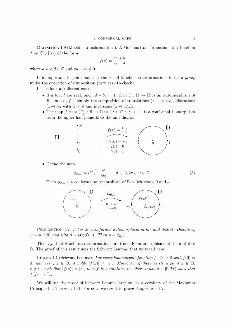
• The map f(z) = i−zi+z : H → D := z ∈ C : |z| < 1 is a conformal isomorphism
from the upper half plane H to the unit disc D.
f (z) = i−zi+z
H
D∞
i
0
0 1−1f(∞) = −1f(i) = 0
f(0) = 1
• Define the map
φϑ,ω := eiϑz − ω1− ωz ϑ ∈ [0, 2π), ω ∈ D . (3)
Then φϑ,ω is a conformal automorphism of D which swaps 0 and ω.
φθ,ω D
1−1
D
0 φθ,ω(ω)
ωφθ,ω(0)
0 7→ ωω 7→ 0
Proposition 1.2. Let φ be a conformal automorphism of the unit disc D. Denote by
ω = φ−1(0) and with ϑ = arg φ′(ω). Then φ = φϑ,ω.
This says that Moebius transformations are the only automorphisms of the unit disc
D. The proof of this result uses the Schwarz Lemma, that we recall here.
Lemma 1.1 (Schwarz Lemma). For every holomorphic function f : D→ D with f(0) =
0, and every z ∈ D, it holds∣∣f(z)
∣∣ ≤ |z|. Moreover, if there exists a point z ∈ D,
z 6= 0, such that∣∣f(z)
∣∣ = |z|, then f is a rotation, i.e. there exists ϑ ∈ [0, 2π) such that
f(z) = eiϑz.
We will see the proof of Schwarz Lemma later on, as a corollary of the Maximum
Principle (cf. Theorem 1.6). For now, we use it to prove Proposition 1.2.
10 1. COMPLEX ANALYSIS PRELIMINARIES
Proof of Proposition 1.2. To see that φ = φϑ,ω, we prove that f := φ φ0,ω is
a rotation by angle ϑ. Note that f(0) = 0 and f is a conformal automorphism on D.
Then by the Schwarz Lemma we have∣∣f(z)
∣∣ ≤ |z| for all z ∈ D \ 0. On the other
hand, f−1 has the same properties: f−1(0) = 0, f conformal automorphism of D and so∣∣f−1(f(z)
)∣∣ ≤ |f(z)| for all z 6= 0, i.e.∣∣f(z)
∣∣ ≥ |z|. We conclude that∣∣f(z)
∣∣ = |z| for all
z ∈ D, so f is a rotation. Check that ϑ = arg φ′(ω) as an exercise.
Exercise 1.1. Show that functions of the form f(z) = az+bcz+d with a, b, c, d real and
ad− bc = 1 are the only conformal automorphisms of H.
So at this point we have classified all automorphisms of D and H.
We conclude with one of the most important results about conformal isomorphisms.
Theorem 1.3 (Riemann mapping Theorem). For all simply connected domains D ( Cthere exists a conformal isomorphism φ : D → D.
Here is a useful corollary.
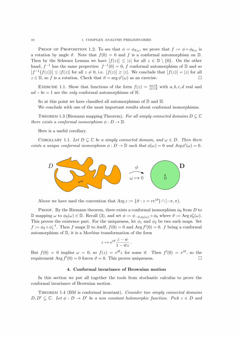
Corollary 1.1. Let D ( C be a simply connected domain, and ω ∈ D. Then there
exists a unique conformal isomorphism φ : D → D such that φ(ω) = 0 and Argφ′(ω) = 0.
D Dφ
ω 0ω 7→ 0
Above we have used the convention that Arg z := ϑ : z = reiϑ ∩ [−π, π).
Proof. By the Riemann theorem, there exists a conformal isomorphism φ0 from D to
D mapping ω to φ0(ω) ∈ D. Recall (3), and set φ := φ−ϑ,φ0(ω) φ0 where ϑ := Argφ′0(ω).
This proves the existence part. For the uniqueness, let φ1 and φ2 be two such maps. Set
f := φ2 φ−11 . Then f maps D to itself, f(0) = 0 and Arg f ′(0) = 0. f being a conformal
automorphism of D, it is a Moebius transformation of the form
z 7→ eiϑz − w1− wz .
But f(0) = 0 implies ω = 0, so f(z) = eiθz for some ϑ. Then f ′(0) = eiϑ, so the
requirement Arg f ′(0) = 0 forces ϑ = 0. This proves uniqueness.
4. Conformal invariance of Brownian motion
In this section we put all together the tools from stochastic calculus to prove the
conformal invariance of Brownian motion.
Theorem 1.4 (BM is conformal invariant). Consider two simply connected domains
D,D′ ( C. Let φ : D → D′ be a non constant holomorphic function. Pick z ∈ D and
4. CONFORMAL INVARIANCE OF BROWNIAN MOTION 11
set z′ = φ(z). Let B be a complex Brownian motion starting from z ∈ D, and define the
stopping time
T := inft ≥ 0 : Bt /∈ D .Moreover, introduce the quantity
T :=
∫ T
0
∣∣φ′(Bs)∣∣2ds ,
and define the new clock
T (t) := infs ≥ 0 :
∫ s
0
∣∣φ′(Bu)∣∣2du = t . (4)
Finally, let
Bt := φ(BT (t)
)be the time-changed image process of B under φ. Then the processes
BT = (Bt)t≤T and BT = (Bt)t≤T
have the same law.
Proof. First of all, we argue that we can assume D to be bounded, and that φ extends
to a C2 function in a neighbourhood of D. Indeed, if this is not the case one can simply
consider an increasing sequence of domains D1 ⊂ · · · ⊂ Dn ⊂ · ⊂ D such that Dn D as
n→∞, and show that all limiting procedures are justified.
Write φ = (f, g) with f = Reφ and g = Imφ. Also writeBt = (Xt, Yt) withXt = ReBtand Yt = ImBt. Since f is C2 (and harmonic) we can use Ito’s formula, that we write in
differential form for simplicity:
df(Xt, Yt) = ∂xf(Xt, Yt)dXt + ∂yf(Xt, Yt)dYt +1
2∂2xxf(Xt, Yt)d〈X〉t+
1
2∂2yyf(Xt, Yt)d〈Y 〉t + ∂2
xyf(Xt, Yt)d〈X,Y 〉t= ∂xf(Xt, Yt)dXt + ∂yf(Xt, Yt)dYt .
To get from the first to the second line above we have used the independence of X and Y ,
and the harmonicity of f . Hence we conclude that f(B) = f(X,Y ) is a local martingale (it
is the integral w.r.t. a local martingale). Similarly, f(B) = f(X,Y ) is a local martingale.
Our goal is to use Levy’s characterization of BM for the process φ(B) = (f(B), g(B)). For
now, we have shown that the components are local martingales. It remains to check that
φ(B) has the right quadratic variation. Check that
• d〈f(B)〉t =
[(∂xf(B)
)2+(∂yf(B)
)2]dt
• d〈g(B)〉t =
[(∂xg(B)
)2+(∂yg(B)
)2]dt
• d〈f(B), g(B)〉t = 0.
Then summing all terms, and using Cauchy-Riemann equations, we get
d〈φ(B)〉t =∣∣φ′(B)
∣∣2dt .

12 1. COMPLEX ANALYSIS PRELIMINARIES
Now to get the conclusion we need a time-change, which makes d〈φ(B)〉t into dt. This is
clearly given by (4): indeed, the reader can check that 〈φ(BT (t))〉 = t. The theorem then
follows by Levy’s characterization of BM.
We list some useful corollaries.
4.1. Corollaries. As a first corollary of the conformal invariance, we can prove that
complex Brownian motion exits any simply connected domain in a finite time.
Corollary 1.2. Let D ( C be any simply connected domain. Pick any point z ∈ D,
and let B = (Bt)t≥0 be a complex Brownian motion started from z. Define
T := inft ≥ 0 : Bt /∈ D
to be the first exit time from D. Then T <∞ almost surely.
As an example, take D = C\z ∈ R : z < 0, the complex plane without half real axis.
Then the above results tells us that complex BM will hit the negative real axis in finite
time. Note that this does not follows from the neighbourhood recurrence of 2-dimensional
BM, since C \D has zero Lebesgue measure.
Proof. By the Riemann mapping theorem, there exists a conformal isomorphism φ
mapping D to the unit disc D with φ(z) = 0. The image process of B under φ is, by
conformal invariance, a time-changed BM starting from 0. We argue by contradiction:
assume that T = ∞, that is: φ(B) takes infinitely longer to reach the boundary of D.
Then there exists a finite time T1 < T such that |φ(Bt)| ≥ 1/2 ∀t ≥ T1. But φ(B) is a
time-changed complex BM, and therefore it is neighbourhood recurrent, so it must come
back inside the disc z : |z| ≤ 1/2 in finite time, which is a contradiction.
The next result states that the value of a harmonic function at any point inside a
bounded domain can be expressed as a suitable average of boundary values.
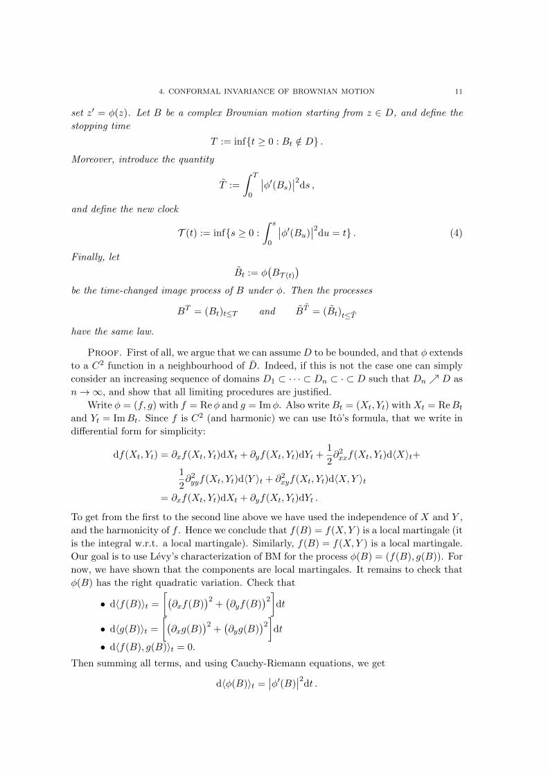
Theorem 1.5 (Kakutani’s formula). Let D ( C be any bounded domain. Let u be
a harmonic function on D which extends continuously to D. Pick any point z ∈ D, and
let B = (Bt)t≥0 be a complex Brownian motion started from z. Define the first exit time
T := inft ≥ 0 : Bt /∈ D from D as before. Then it holds
u(z) = Ez(u(BT )
).
z = B0
BT
D
4. CONFORMAL INVARIANCE OF BROWNIAN MOTION 13
Proof. The strategy of the proof is the following. If u is C2 in a neighbourhood of D,
then the thesis follows easily by Ito’s formula and the Optional Stopping Theorem (OST).
For the general case, we approximate D by an increasing sequence of domains Dn D in
which the previous point applies, and then use the continuity of BM to conclude. Let us
now implement this strategy.
Suppose first that u is C2 in a neighbourhood of D. Then we apply Ito’s formula for t ≤ Tto get
u(Bt) = u(B0) +
∫ t
0∇u(Bs)dBs +
1
2
∫ t
0∆u(Bs)︸ ︷︷ ︸
0
ds
= u(z) +
∫ t
0∇u(Bs)dBs .
We conclude that(u(Bt)
)t≤T is a local martingale. We stop it at time T to make it
bounded. But any bounded local martingale is a (bounded) true martingale, so we con-
clude that(u(Bt∧T )
)t≥0
is a (bounded) true martingale. By the OST, then, we have
u(z) = u(B0) = Ez(u(BT )
).
This concludes the proof for u ∈ C2(D). To deal with the general case, let Dn D be,
say, the increasing sequence of domains
Dn := z ∈ D : dist(z∂D) > 1/n .Then u ∈ C2(Dn), and for all z ∈ Dn it holds
u(z) = Ez(u(BTn)
)where Tn is the first exit time of B from Dn. It is straightforward to check that Tn T
almost surely which, together with the continuity of both B and the function u, gives
limn→∞
u(BTn) = u(BT ) almost surely.
It only remains to swap limit and expectation, but this is allowed since u is continuous
on the bounded closed domain D, and hence it is bounded. We conclude that by the
Dominated Convergence Theorem (DTC) it holds
u(z) = Ez(
limn→∞
u(BTn))
= Ez(u(BT )
).
As a first consequence of Kakutani’s formula, we see that for u and D as in the
Theorem, it holds
u(z) ≤ supw∈∂D
u(w) .
On a more interesting note, we obtain the mean value property of harmonic func-
tions, which goes as follows. Let u be harmonic in D. Then for all z ∈ D, and all R > 0
small enough so that the ball BR(z) of radius R centred at z is contained in D, it holds
u(z) = Ez(u(BT (BR(z)))
)=
1
2π
∫ 2π
0u(z +Reiϑ)dϑ
14 1. COMPLEX ANALYSIS PRELIMINARIES
where T (BR(z)) denotes the first exit time from the ball BR(z). We remark that the mean
value property is also sufficient for a function to be harmonic in a given domain.
The following very useful result says that harmonic functions attain their maximum
on the boundary.
Theorem 1.6 (Maximum principle). Let u be harmonic in a domain D, and suppose
that there exists z ∈ D such that u(z) ≥ u(w) for all w ∈ D. Then u is constant in D.
Proof. Let m = u(z), and define the set D := w ∈ D : u(w) = m to be the set of
points at which the maximum is attained. Then:
• D is non empty (it contains at least z),
• D is closed inD, since it is the pre-image of the closed set m under a continuous
function,
• D is open in D, because if z0 ∈ D then we can apply the mean value property
to conclude that u must be identically m in a small neighbourhood of z0.
But the above implies that D is the whole D, which is what we wanted to show.
5. Density of harmonic measure
Let D be a simply connected domain, and denote by ∂D its boundary. Let z /∈ D be
a point strictly outside D, and let (Bt)t≥0 be a standard Brownian Motion on C starting
from z. Let T := inft ≥ 0 : BT ∈ D, and assume that ∂D is nice enough so that for any
arc γ ⊆ ∂D we have
Pz(BT ∈ γ) =
∫γhD(z, w)dw.
In this case hD(z, ·) is referred to as the density of harmonic measure on ∂D seen from z.
As an example, we note that by rotation invariance of Brownian Motion
hD(0, w) = hD(∞, w) =1
2π.
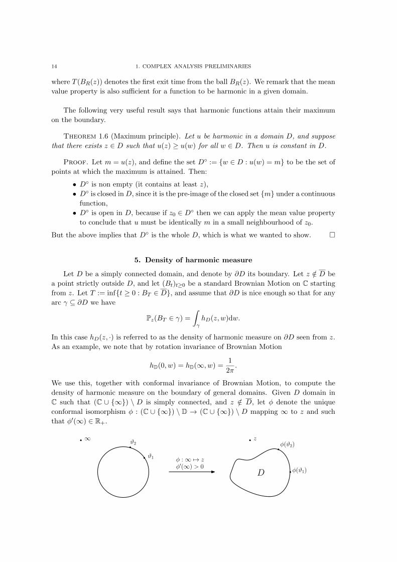
We use this, together with conformal invariance of Brownian Motion, to compute the
density of harmonic measure on the boundary of general domains. Given D domain in
C such that (C ∪ ∞) \ D is simply connected, and z /∈ D, let φ denote the unique
conformal isomorphism φ : (C ∪ ∞) \ D → (C ∪ ∞) \ D mapping ∞ to z and such
that φ′(∞) ∈ R+.
φ : ∞ 7→ zφ′(∞) > 0
∞ z
D
ϑ1
ϑ2
φ(ϑ1)
φ(ϑ2)
5. DENSITY OF HARMONIC MEASURE 15
Pick any 0 ≤ ϑ1 < ϑ2 < 2π. Then by conformal invariance of Brownian Motion we
haveϑ2 − ϑ1
2π= hD(∞, [eiϑ1 , eiϑ2 ]) = hD(z, [φ(eiϑ1), φ(eiϑ2)])
=
∫ φ(eiϑ2 )
φ(eiϑ1 )hD(z, w)dw = `([φ(eiϑ1), φ(eiϑ2)]) · hD(z, φ(eiϑ0)),
for some ϑ0 ∈ [ϑ1, ϑ2], where `(γ) denotes the arc length of a curve γ and the last equality
follows from the mean values theorem. We now divide both sides by ϑ2 − ϑ1 and let
ϑ2 ϑ1 to get 12π = |φ′(eiϑ1)| · hD(z, φ(eiϑ1)). This tells us that
hD(z, φ(eiϑ1)) =1
2π|φ′(eiϑ1)|−1.
The fact that the density of harmonic measure at φ(eiϑ) seen from z is inversely pro-
portional to |φ′(eiϑ1)| will be very useful to gain intuition on the effect of distortion in
Hastings–Levitov clusters.

CHAPTER 2
Hastings–Levitov models
The question of obtaining a rigorous description of spatial growth phenomena observed
in nature has received much attention in the last few decades in the mathematical com-
munity. One possible approach to this problem, on which we focus here, is to model the
growth as the result of subsequent aggregation of particles, which randomly move in the
surrounding space. We refer to such dynamics as random aggregation.
1. Discrete aggregation models
A random aggregation model consists of an underlying infinite graph together with
an aggregation rule. We focus here on deterministic, planar, undirected graphs, on whose
vertex set the particles live. Say that a vertex v of the graph is filled if it is occupied
by exactly one particle, and v is empty otherwise. Starting from one particle (i.e. filled
vertex), we grow increasing clusters of particles by aggregating one vertex at the time,
according to the prescribed aggregation rule. When a vertex is added to the cluster we
declare it filled, so that the cluster coincides with the set of filled vertices.
1.1. The Eden model. Arguably, the simplest of such models is the so called Eden
model [Ede61], introduced by Eden in 1961, according to which at each step one empty
site adjacent to the cluster is chosen uniformly at random, and added to the cluster. More
precisely, let the underlying graph be the d–dimensional lattice Zd, and take the initial
cluster to be the singleton E(0) = 0. Define a family of growing clusters (E(n))n≥0
recursively as follows. Write u ∼ v if u is adjacent to v, that is |u− v| = 1, and let
∂E(n− 1) = v /∈ E(n− 1) : v ∼ u for some u ∈ E(n− 1)denote the outer boundary of the set E(n− 1). Then, if ωn is a uniformly chosen element
of ∂E(n− 1), set
E(n) = E(n− 1) ∪ ωn.For such family of growing clusters it is natural to ask if there is a limiting shape as the
number of particles diverges, i.e. as n → ∞. This question was settled by Richardson in
[Ric73], showing that there exists indeed a limiting shape, and it is compact and convex
(see also [CD81, Kes93]). The problem of determining the limiting shape remains open.
1.2. Diffusion Limited Aggregation. A variant of the Eden model was introduced
a few years later by the physicists Witten and Sander [WJS81, WJS83], seeking to
explain the formation of arms, or dendrites, in metal–particles aggregation. This is the
celebrated Diffusion Limited Aggregation, in short DLA, and it is defined similarly to the
Eden model, with the crucial difference that the position of the next added particle is
17
18 2. HASTINGS–LEVITOV MODELS
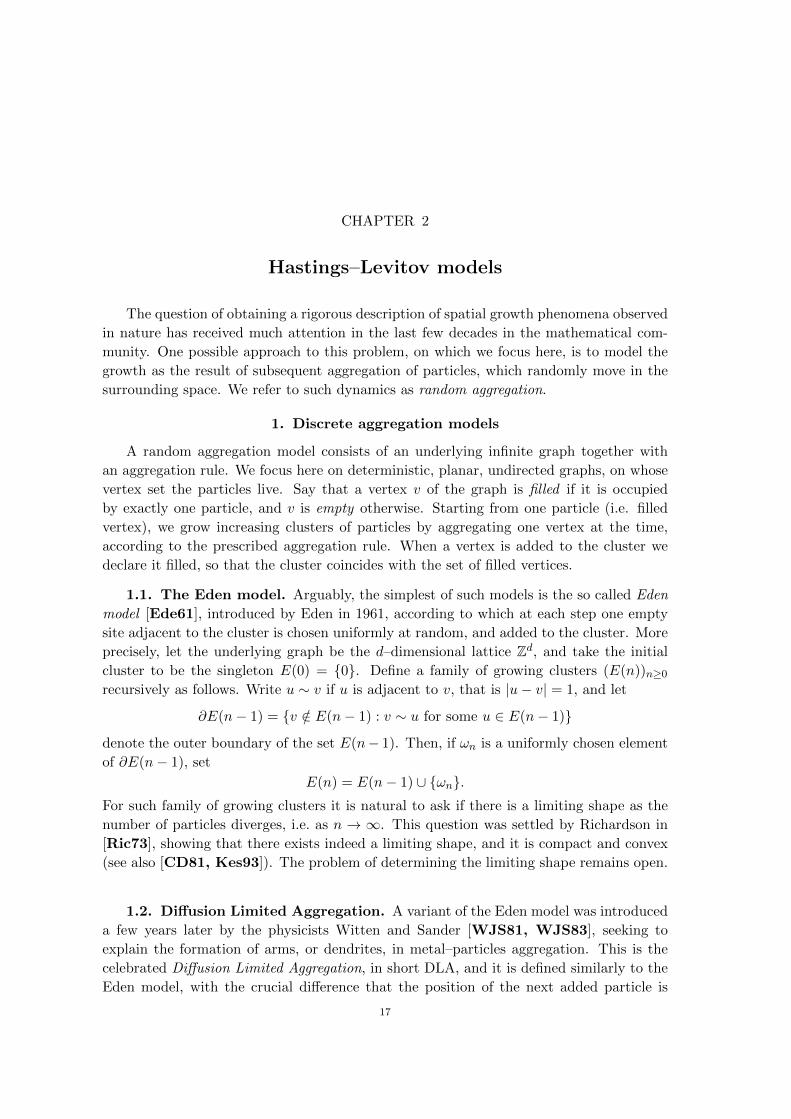
Figure 1. A large Eden cluster (simulation by Jason Miller).
chosen according to the harmonic measure of the outer boundary of the cluster seen from
infinity, rather than according to the uniform measure on the same set. More precisely, at
each integer time n ≥ 1 we start a simple symmetric random walk ω(n) = (ω(n)(t))t≥0 on Zdfrom infinity, independent of everything else, and let τn := inft ≥ 0 : ω(n)(t) ∈ ∂D(n−1)denote the first time the walk reaches the outer boundary of D(n− 1). Then set
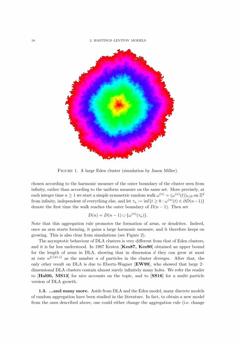
D(n) = D(n− 1) ∪ ω(n)(τn).Note that this aggregation rule promotes the formation of arms, or dendrites. Indeed,
once an arm starts forming, it gains a large harmonic measure, and it therefore keeps on
growing. This is also clear from simulations (see Figure 2).
The asymptotic behaviour of DLA clusters is very different from that of Eden clusters,
and it is far less understood. In 1987 Kesten [Kes87, Kes90] obtained an upper bound
for the length of arms in DLA, showing that in dimension d they can grow at most
at rate n2/(d+1) as the number n of particles in the cluster diverges. After that, the
only other result on DLA is due to Ebertz-Wagner [EW99], who showed that large 2–
dimensional DLA clusters contain almost surely infinitely many holes. We refer the reader
to [Hal00, MS13] for nice accounts on the topic, and to [SS16] for a multi–particle
version of DLA growth.
1.3. ...and many more. Aside from DLA and the Eden model, many discrete models
of random aggregation have been studied in the literature. In fact, to obtain a new model
from the ones described above, one could either change the aggregation rule (i.e. change
2. A CONTINUUM MODEL: HASTINGS–LEVITOV GROWTH 19
Figure 2. A large DLA cluster (simulation by Vincent Beffara).
the measure with respect to which the location of the new added particle is chosen), or
change the underlying graph on which the particles live, or change both. An example of
aggregation rule change is given by the Internal DLA (IDLA) [DF91, LBG92, JLS14a,
JLS14b, JLS13, JLS12, AG10, AG13a, AG13b, AG14], where the location of the
next added particle is sampled according to the harmonic measure of the outer boundary of
the cluster seen from the origin. Other important examples are the Dielectric Breakdown
Models of parameter γ > 0, in short DBMγ , according to which the location of the next
particle is sampled from the γth power of the harmonic measure of the outer boundary
of the cluster seen from infinity [NPW84]. Thus γ = 0 corresponds to the Eden model,
γ = 1 to DLA, and γ ∈ (0, 1) interpolates between the two. Finally, we would like to
mention DLA on cylinder graphs [BY08] and on regular trees [BPP97], Directed DLA
[Mar14], Stretched IDLA [BKP12], Diffusion Limited Deposition [ACSS16] and First
Passage Percolation [HW65, Kes86, Kes03, CD81, Mar04] (see also the recent survey
[AHD15] and references therein).
2. A continuum model: Hastings–Levitov growth
A common feature of some of the discrete aggregation models described above (e.g.
Eden model and DLA) is that their asymptotic properties, such as the limiting shape
and Hausdorff dimension, have been numerically found to depend on the underlying lat-
tice structure (see for example [BBRT85, MBRS87], where simulations of such models

20 2. HASTINGS–LEVITOV MODELS
are discussed). This led researchers to look, in the late 1980’s, for off–lattice analogues
[Roh11]. In 2000 Carleson and Makarov [CM01] introduced a deterministic growth
model on the complex plane, defined in terms of Loewner flows driven by time-dependent
measures on the unit circle. Following their ideas, Hastings and Levitov [HL98] proposed
a one parameter family of random growth models, now called HL(α) for α ∈ [0,∞). These
lecture notes are concerned with the study of the α = 0 case, that we now describe.
Figure 3. HL(0) cluster with 500 particles (simulation by Henry Jackson).
2.1. The HL(0) model. Let D denote the open unit disc in the complex plane, and
let K0 = D be the initial cluster. We grow an increasing family K0 ⊂ K1 ⊂ K2 . . . of
compact subsets of the complex plane, that we call clusters, as follows. Fix P ⊂ C \ Dto be a (non–empty) connected compact set having 1 as a limit point, and such that
the complement of K = D ∪ P in C ∪ ∞ is simply connected. We regard P as the
basic particle. For concreteness, note that the slit P = [1, 1 + δ] satisfies all the above
assumptions (this is indeed the particle shape used in all HL(0) simulations included in
these notes).
At each step, a new particle Pn, consisting of a distorted copy of P , attaches to the
cluster Kn−1 according to the following growth mechanism. Let D0 = (C∪∞)\K0 and
D = (C ∪ ∞) \K. Then by Theorem 1.3 there exists a unique conformal isomorphism
F : D0 → D such that F (∞) =∞ and F ′(∞) ∈ R>0. Set G = F−1, and let (Θn)n≥1 be a
sequence of i.i.d. random variables with Θn ∼Uniform[−π, π).
2. A CONTINUUM MODEL: HASTINGS–LEVITOV GROWTH 21
F P1 + δ1
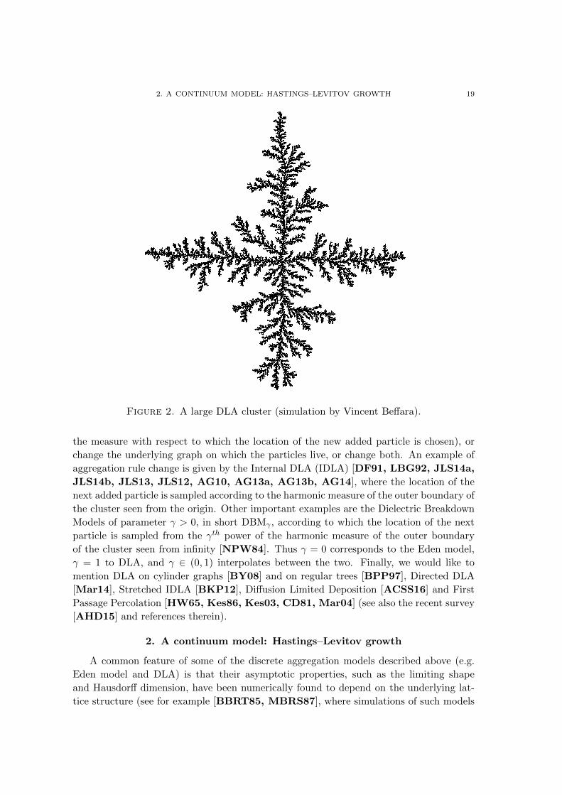
Figure 4. The conformal map F attaching the particle P = [1, 1 + δ] at 1.
Define
Fn(z) := eiΘnF (e−iΘnz) , Gn(z) = F−1n (z) .
Then the map Fn attaches the particle P to the unit disc at the uniformly chosen point
eiΘn . Define Φn(z) := F1 · · · Fn(z), Dn = Φn(D0) and Kn = (C ∪ ∞) \Dn. We say
that the conformal map Φn grows an HL(0) cluster up to the n-th particle, while Γn = Φ−1n
maps it out. Note that, by conformal invariance, choosing the attachment angles to be
uniformly distributed corresponds to choosing the attachment point of the n-th particle
according to the harmonic measure of the boundary of the cluster Kn−1 seen from infinity.
With this notation, then, one has
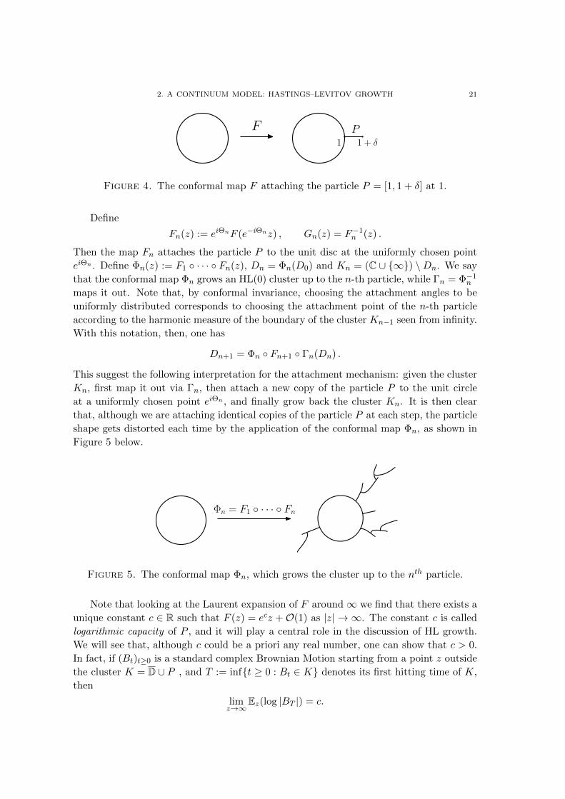
Dn+1 = Φn Fn+1 Γn(Dn) .
This suggest the following interpretation for the attachment mechanism: given the cluster
Kn, first map it out via Γn, then attach a new copy of the particle P to the unit circle
at a uniformly chosen point eiΘn , and finally grow back the cluster Kn. It is then clear
that, although we are attaching identical copies of the particle P at each step, the particle
shape gets distorted each time by the application of the conformal map Φn, as shown in
Figure 5 below.
Φn = F1 · · · Fn
Figure 5. The conformal map Φn, which grows the cluster up to the nth particle.
Note that looking at the Laurent expansion of F around∞ we find that there exists a
unique constant c ∈ R such that F (z) = ecz +O(1) as |z| → ∞. The constant c is called
logarithmic capacity of P , and it will play a central role in the discussion of HL growth.
We will see that, although c could be a priori any real number, one can show that c > 0.
In fact, if (Bt)t≥0 is a standard complex Brownian Motion starting from a point z outside
the cluster K = D ∪ P , and T := inft ≥ 0 : Bt ∈ K denotes its first hitting time of K,
then
limz→∞
Ez(log |BT |) = c.
22 2. HASTINGS–LEVITOV MODELS
This is a consequence of Proposition 3.1 below, and it shows that the logarithmic capacity
is related to the size of the particle P . Indeed, the only positive contribution to the
expectation comes from Brownian trajectories hitting K on P , and the larger is P the
larger is such expectation, and hence c. We will use the logarithmic capacity as a measure
of the size of the particle throughout, and look at the small particle limit c→ 0.
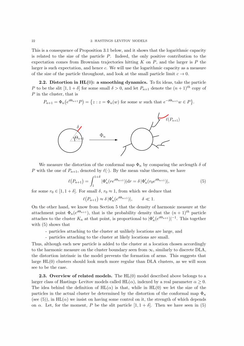
2.2. Distortion in HL(0): a smoothing dynamics. To fix ideas, take the particle
P to be the slit [1, 1 + δ] for some small δ > 0, and let Pn+1 denote the (n+ 1)th copy of
P in the cluster, that is
Pn+1 = Φn
(eiΘn+1P
)=z : z = Φn(w) for some w such that e−iΘn+1w ∈ P
.
ΦnΘn+1
δ
`(Pn+1)
We measure the distortion of the conformal map Φn by comparing the arclength δ of
P with the one of Pn+1, denoted by `(·). By the mean value theorem, we have
`(Pn+1
)=
∫ 1+δ
1|Φ′n(reiΘn+1)|dr = δ |Φ′n(r0e
iΘn+1)|, (5)
for some r0 ∈ [1, 1 + δ]. For small δ, r0 ≈ 1, from which we deduce that
`(Pn+1
)≈ δ |Φ′n(eiΘn+1)|, δ 1.
On the other hand, we know from Section 5 that the density of harmonic measure at the
attachment point Φn(eiΘn+1), that is the probability density that the (n + 1)th particle
attaches to the cluster Kn at that point, is proportional to |Φ′n(eiΘn+1)|−1. This together
with (5) shows that
- particles attaching to the cluster at unlikely locations are large, and
- particles attaching to the cluster at likely locations are small.
Thus, although each new particle is added to the cluster at a location chosen accordingly
to the harmonic measure on the cluster boundary seen from∞, similarly to discrete DLA,
the distortion intrinsic in the model prevents the formation of arms. This suggests that
large HL(0) clusters should look much more regular than DLA clusters, as we will soon
see to be the case.
2.3. Overview of related models. The HL(0) model described above belongs to a
larger class of Hastings–Levitov models called HL(α), indexed by a real parameter α ≥ 0.
The idea behind the definition of HL(α) is that, while in HL(0) we let the size of the
particles in the actual cluster be determined by the distortion of the conformal map Φn
(see (5)), in HL(α) we insist on having some control on it, the strength of which depends
on α. Let, for the moment, P be the slit particle [1, 1 + δ]. Then we have seen in (5)
2. A CONTINUUM MODEL: HASTINGS–LEVITOV GROWTH 23
that for δ 1 the size (meaning arc length) of the particle Pn+1 in the actual cluster is
roughly δ|Φ′n(eiΘn+1)|. To cancel this distortion factor, one could therefore attach a slit of
(random) length δn+1 = δ/|Φ′n(eiΘn+1)|, which will result in a particle of size roughly δ in
the actual cluster. In general, one can vary the strength of such rescaling by introducing
a parameter α > 0 and setting
δn+1 =δ
|Φ′n(eiΘn+1)|α/2 .
Although the above considerations are specific to the slit particle, the same reasoning
can be carried out for more general particle shapes after replacing the arc length by
the logarithmic capacity. Indeed, Norris and Turner show in [NT12] that, in the small
particle limit, the logarithmic capacity of the particle equals (up to absolute multiplicative
constants) the square of its diameter (cf. Corollary 3.1). Thus for general particle shape P
we define the HL(α) model as obtained from HL(0) by attaching, at each step, a rescaled
copy of the basic particle P of logarithmic capacity
cn+1 =c
|Φ′n(eiΘn+1)|α . (6)
Note that α = 2 will result in particles having roughly the same size in the actual cluster.
Since the attachment point is chosen according to harmonic measure from∞, then, HL(2)
seems to be a good off-lattice analogous to discrete DLA. For α > 2, the size of the
particles in the actual cluster becomes proportional to a power of the harmonic measure
of the cluster boundary near the attachment point. This favours the growth of arms, since
to region of high harmonic measure we attach large particles (here by large we mean larger
than what they would have been without the α > 0 regularization). For α ∈ (0, 2), on the
other hand, the α regularization really contrasts the effect of distortion, since the size of
particles in the actual cluster becomes inversely proportional to a power of the density of
harmonic measure close to the attachment point. In fact, the regime α ∈ [1, 2] seems to be
the most interesting from the point of view of modelling real phenomena. Indeed, recall
the definition of Dielectric Breakdown Model (DBM in short) from Section 1.3. Then by
comparing local growth rates Hastings and Levitov argue that for α ∈ [1, 2] the HL(α)
model should be the right off–lattice analogue to DBMα−1, thus in particular recovering
the Eden model for α = 1 and DLA for α = 2. Let us explain this point in more detail.
Recall that in (discrete) DBMη at each step we choose the attachment location of the next
particle on the outer boundary of the cluster according to the ηth power of the harmonic
measure of the cluster boundary seen from infinity, which is roughly |Φ′n(z)|−η. At this
location we attach a particle of fixed size, say c. Thus the rate of growth of the cluster
boundary around a point z is roughly given by
Growth rate of DBMη at z ≈ c |Φ′n(z)|−η.
For HL(α), on the other hand, the rate of growth around z is given by the probability
of attaching a particle at z, roughly |Φ′n(z)|−1, times the size of the attached particle,
roughly c |Φ′n(z)|2−α (see (5)-(6)). Thus
Growth rate of HL(α) at z ≈ c |Φ′n(z)|1−α.
24 2. HASTINGS–LEVITOV MODELS
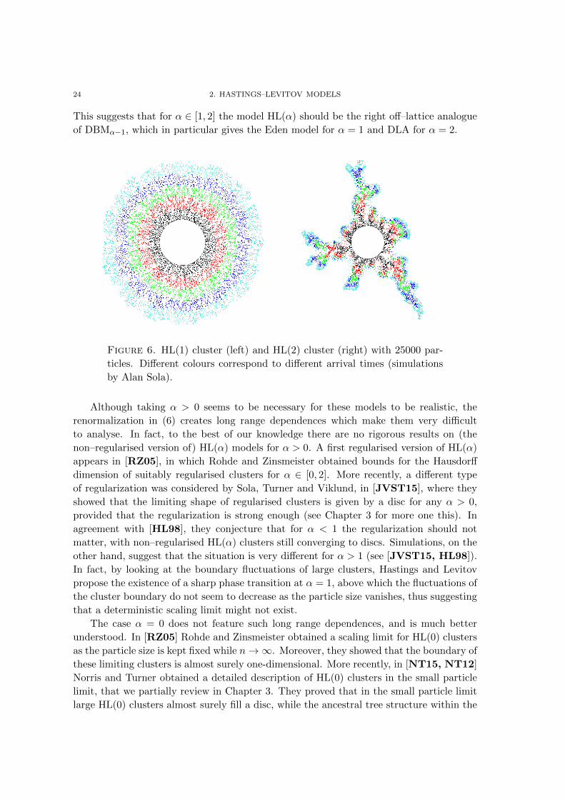
This suggests that for α ∈ [1, 2] the model HL(α) should be the right off–lattice analogue
of DBMα−1, which in particular gives the Eden model for α = 1 and DLA for α = 2.
Figure 6. HL(1) cluster (left) and HL(2) cluster (right) with 25000 par-
ticles. Different colours correspond to different arrival times (simulations
by Alan Sola).
Although taking α > 0 seems to be necessary for these models to be realistic, the
renormalization in (6) creates long range dependences which make them very difficult
to analyse. In fact, to the best of our knowledge there are no rigorous results on (the
non–regularised version of) HL(α) models for α > 0. A first regularised version of HL(α)
appears in [RZ05], in which Rohde and Zinsmeister obtained bounds for the Hausdorff
dimension of suitably regularised clusters for α ∈ [0, 2]. More recently, a different type
of regularization was considered by Sola, Turner and Viklund, in [JVST15], where they
showed that the limiting shape of regularised clusters is given by a disc for any α > 0,
provided that the regularization is strong enough (see Chapter 3 for more one this). In
agreement with [HL98], they conjecture that for α < 1 the regularization should not
matter, with non–regularised HL(α) clusters still converging to discs. Simulations, on the
other hand, suggest that the situation is very different for α > 1 (see [JVST15, HL98]).
In fact, by looking at the boundary fluctuations of large clusters, Hastings and Levitov
propose the existence of a sharp phase transition at α = 1, above which the fluctuations of
the cluster boundary do not seem to decrease as the particle size vanishes, thus suggesting
that a deterministic scaling limit might not exist.
The case α = 0 does not feature such long range dependences, and is much better
understood. In [RZ05] Rohde and Zinsmeister obtained a scaling limit for HL(0) clusters
as the particle size is kept fixed while n→∞. Moreover, they showed that the boundary of
these limiting clusters is almost surely one-dimensional. More recently, in [NT15, NT12]
Norris and Turner obtained a detailed description of HL(0) clusters in the small particle
limit, that we partially review in Chapter 3. They proved that in the small particle limit
large HL(0) clusters almost surely fill a disc, while the ancestral tree structure within the
2. A CONTINUUM MODEL: HASTINGS–LEVITOV GROWTH 25
cluster converges, always in the small particle limit, to the Brownian Web [FINR04].
This provides an interesting connection between these two a priori unrelated models.
A promising variant of Hastings–Levitov growth is the so called Angular Loewner
Evolution of parameter η, ALE(0, η) in short, which keeps the HL(0) distortion but adjusts
the rate at which particles are added to the cluster to compensate for it. Indeed, we saw
that in HL(0) growth large particles are attached to regions of low harmonic measure, and
small particles are attached to regions of high harmonic measure. To compensate this, we
could think of attaching particles to regions of low harmonic measure at a lower rate, and to
regions of high harmonic measure to a higher rate. More precisely, to balance the distortion
factor |Φ′n(eiΘn+1)| we attach particles around eiΘn+1 at rate |Φ′n(eiΘn+1)|−1, that is at a
rate which is directly proportional to the local density of harmonic measure. In general, in
ALE(0, η) at each step we attach a particle of constant logarithmic capacity c, at a random
point eiΘn+1 drawn from a probability density function proportional to |Φ′n(eiΘn+1)|1−η. A
regularised version of this model is studied by Sola, Turner and Viklund in a forthcoming
paper.

CHAPTER 3
Small particle limit
In this Chapter we review the scaling limit result of Norris and Turner [NT12], stating
that as the number of particles diverges and their size converges to 0, large HL(0) clusters
converge to disks. Recall that we take the basic particle P ⊂ C \ D to be a (non–
empty) connected compact set having 1 as a limit point, and such that the complement of
K = D∪P in C∪∞ is simply connected. We make the following additional assumptions
on P throughout.
Assumption 1. The basic particle P is such that the unique map F : D0 → D extends
continuously to D0 = z ∈ C : |z| ≥ 1. Moreover, there exists δ > 0 such that
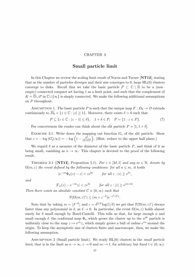
P ⊆ z ∈ C : |z − 1| ≤ δ, 1 + δ ∈ P, P = z : z ∈ P. (7)
For concreteness the reader can think about the slit particle P = [1, 1 + δ].
Exercise 3.1. Write down the mapping out function Gs of the slit particle. Show
that c = − log |G′s(∞)| = − log(
1− δ2
(2+δ)2
). (Hint: reduce to the upper half plane.)
We regard δ as a measure of the diameter of the basic particle P , and think of it as
being small, vanishing as n → ∞. This chapter is devoted to the proof of the following
result.
Theorem 3.1 ([NT12], Proposition 5.1). For ε ∈ [2δ, 1] and any m ∈ N, denote by
Ω(m, ε) the event defined by the following conditions: for all n ≤ m, it holds
|e−cnΦn(z)− z| < εe6ε for all z : |z| ≥ e5ε,
and
|Γn(z)− e−cnz| < εe5ε for all z : |z| ≥ ecn+4ε.
Then there exists an absolute constant C ∈ (0,∞) such that
P(Ω(m, ε)c) ≤ (m+ ε−2)e−ε3/Cc.
Note that by taking m = bδ−6c and ε = δ2/3 log(1/δ) we get that P(Ω(m, ε)c) decays
faster than any polynomial in δ, as δ → 0. In particular, the event Ω(m, ε) holds almost
surely for δ small enough by Borel-Cantelli. This tells us that, for large enough n and
small enough δ, the conformal map Φn which grows the cluster up to the nth particle is
uniformly close to the map z 7→ ecnz, which simply grows a ball of radius ecn around the
origin. To keep the asymptotic size of clusters finite and macroscopic, then, we make the
following assumption.
Assumption 2 (Small particle limit). We study HL(0) clusters in the small particle
limit, that is in the limit as n→∞, c→ 0 and nc→ t, for arbitrary but fixed t ∈ (0,∞).
27
28 3. SMALL PARTICLE LIMIT
This assumption will be in force throughout these lecture notes, so that when we write
n→∞ or c→ 0 we in fact mean the above.
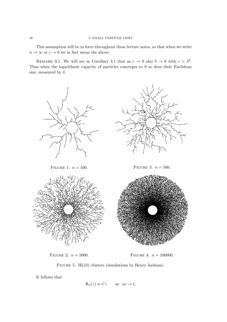
Remark 3.1. We will see in Corollary 3.1 that as c → 0 also δ → 0 with c δ2.
Thus when the logarithmic capacity of particles converges to 0 so does their Euclidean
size, measured by δ.
Figure 1. n = 100.
Figure 2. n = 5000.
Figure 3. n = 500.
Figure 4. n = 100000.
Figure 5. HL(0) clusters (simulations by Henry Jackson).
It follows that
Φn(z) ≈ etz as nc→ t,
3. SMALL PARTICLE LIMIT 29
which shows that the map that grows the n–particles cluster is close, in the small particle
limit, to the map that grows an Euclidean ball of radius et around the origin. In this sense
we say that the scaling limit of HL(0) clusters is an Euclidean ball.
Remark 3.2. Although one can let |z| → 1 as n → ∞ in Theorem 3.1 of Norris and
Turner, the limiting shape result breaks down (and it should) if |z| → 1 too fast with
respect to δ. On the other hand, we will show in Chapter 4 that it does not break too
much: it still holds in the sense of distributions, for a suitably small space of test functions.
The analysis carried out by Norris and Turner in [NT12] is rather sophisticated, and it
gives much more information than what stated in Theorem 3.1. In particular, it provides
very accurate estimates on the distortion of the conformal map Φn, that are crucial for
the analysis of fluctuations. On the other hand, the limiting shape of large clusters can
be guessed by very simple heuristic arguments.
Heuristics: a Loewner flow argument. The heuristics presented below is inspired
by the discussion of anisotropic Hastings–Levitov models of Sola, Turner and Viklund in
[JVST15], and it provides an exact guess for the limiting shape.
The main observation is that, if P is the slit particle P = [1, 1 + δ], then Hastings–
Levitov clusters are Loewner hulls associated to the Loewner flow driven by a specific
random measure, consisting of Dirac masses at the attachment points. More precisely,
recall that (Θk)k≥1 denotes the sequence of attachment angles, and define
ξn(t) :=n∑k=1
eiΘk1[c(k−1),ck)(t).
Let (ft)t≥0 be the Loewner flow driven by the random measure δξn(t), where δx denote the
Dirac delta measure centred at x, i.e.
∂tft(z) = zf ′t(z)
∫|z|=1
z + ζ
z − ζ dδξn(t)(ζ), f0(z) = z. (8)
Then Φn(z) = fnc(z) for the slit particle P = [1, 1 + δ]. Using the Loewner equation (8)
for ft, we find
∂tft(z) = zf ′t(z)
∫|z|=1
z + ζ
z − ζ
( n∑k=1
dδeiΘk (ζ)1[c(k−1),ck)(t)
)
= zf ′t(z)
n∑k=1
(∫|z|=1
z + ζ
z − ζ dδeiΘk (ζ)
)1[c(k−1),ck)(t)
= zf ′t(z)
n∑k=1
z + eiΘk
z − eiΘk 1[c(k−1),ck)(t).
Now, if we assume that there exists a deterministic scaling limit, then the random sum
appearing in the last term above should converge to a deterministic limit itself. To get an
30 3. SMALL PARTICLE LIMIT
idea of how this limit should look like, we compute its expectation:
E( n∑k=1
z + eiΘk
z − eiΘk 1[c(k−1),ck)(t)
)=
n∑k=1
E(z + eiΘk
z − eiΘk)
1[c(k−1),ck)(t)
= E(z + eiΘ1
z − eiΘ1
)=
∫|z|=1
z + ζ
z − ζdζ
2π= 1.
Thus if there is a deterministic limit for the random map Φn = fnc, then it must coincide
with the solution ft to ∂ft(z) = zf ′t(z)
f0(z) = z
evaluated at time t = nc. The above is easy to solve, to get ft(z) = etz. Thus we conclude
that if there exists a random conformal map ft such that Φn → ft as n→∞, nc→ t, then
it must be ft(z) = etz.
1. Preliminary estimates
In order to prove Theorem 3.1, and throughout the course, we will need to understand
how much the conformal maps Φn,Γn move points around. To this end, we look at
distortion estimates for the basic maps F,G. To start with, note that:
(P1) |F (z)| > |z| for all z ∈ D0, |G(z)| < |z| for all z ∈ D,
(P2) there exists a constant C > 0 such that |F (z)| ≤ C|z| for all z ∈ D0 and |G(z)| ≥|z|/C for all z ∈ D.
Indeed, (P1) follows from Schwarz lemma (cf. Lemma 1.1), while (P2) is a consequence
of the prescribed behaviour at infinity for F,G. In order to get more refined estimates, it
turns out to be useful to look at F,G in logarithmic coordinates. To this end, note that the
holomorphic functions F (z)/z and G(z)/z are non–zero on D0 and D respectively, with
a controlled behaviour at infinity. It follows that we can define their complex logarithm
on the same domains, to get the holomorphic functions logF (z)/z and logG(z)/z. We fix
the branch by requiring that logF (z)/z → c and logG(z)/z → c as |z| → ∞.
The following result appears in [NT12] (cf. Proposition 4.1 and Corollary 4.2 therein).
Proposition 3.1. There exists an absolute constant C <∞ such that, for all z ∈ D:
|z − 1| > 2δ, the following hold:∣∣∣∣ logG(z)
z+ c
∣∣∣∣ ≤ Cc
|z − 1| ,∣∣∣∣ d
dzlog
G(z)
z
∣∣∣∣ ≤ Cc
|z − 1|2 . (9)
Remark 3.3 (Geometric interpretation of c). Write log G(z)z = u(z) + iv(z). Then u, v
are bounded harmonic functions on D. It follows that if (Bt)t≥0 is a standard Brownian
Motion on D starting at z ∈ D, then (u(Bt))t≥0 and (v(Bt))t≥0 are continuous martingales.
Let T = inft ≥ 0 : Bt /∈ D denote the first hitting time of the boundary of the cluster.
Then T <∞ almost surely, and we can use the Optional Stopping theorem to see that
u(z) = E(u(B0)) = E(u(BT )) = E(
log|G(BT )||BT |
)= −E(log |BT |).

1. PRELIMINARY ESTIMATES 31
On the other hand, we know that lim|z|→∞ u(z) = lim|z|→∞ log G(z)z = log e−c = −c. We
therefore conclude that
c = lim|z|→∞
E(log |BT |). (10)
In particular, this tells us that c ≥ 0, which was not a priori clear. We will see in the
proof of Proposition 3.1 that in fact c > 0. Moreover, (10) shows that the logarithmic
capacity c of a particle P is closely related to the size of the particle. Indeed, the only
contribution to the expectation comes from Brownian trajectories hitting the cluster on
P , so that |BT | > 1, and the larger the particle P , the larger the expectation, and hence
c.
z
BT
The next corollary shows that, in fact, the relationship between c and the Euclidean
size of P can be made more precise.
Corollary 3.1. It holdsδ2
6≤ c ≤ 3δ2
4(11)
for δ small enough.
In light of (11) we use c and δ interchangeably, and all statements are intended to hold
for c, δ small enough (recall that we are looking at the small particle limit).
We can now proceed with the proof of Proposition 3.1.
Proof. Let u, v denote the real and imaginary part of log G(z)z respectively, so that
they are harmonic functions on D. Then by optional stopping u(z) = −E(log |BT |) < 0,
T being the first hitting time of K for a Brownian Motion B starting from z. Introduce
the particle P1 ⊃ P defined by P1 =z ∈ D0 :
∣∣ z−1z+1
∣∣ ≤ r
, for r = δ/(2 − δ), and set
D1 = (C ∪ ∞) \ (D ∪ P1). Then the unique conformal map G1 : D1 → D0 satisfying
G1(∞) =∞ and G′1(∞) > 0 is given by
G1(z) =z(γz − 1)
z − γ for γ =1− r2
1 + r2. (12)
Set F1 = G−11 , and A = z ∈ ∂P1 : |z| > 1. Then G1(A) = eiϑ : |ϑ| < ϑ0 with ϑ0 =
cos−1 γ. Moreover, u F1 is harmonic and bounded on D0 and, using that 12π
∫|ϑ|≤ϑ0
(u F1)(eiϑ)dϑ = −c, the optional stopping theorem yields
(u F1)(z) = −c+1
2π
∫|ϑ|≤ϑ0
(u F1)(eiϑ) Re( 2eiϑ
z − eiϑ)
dϑ .
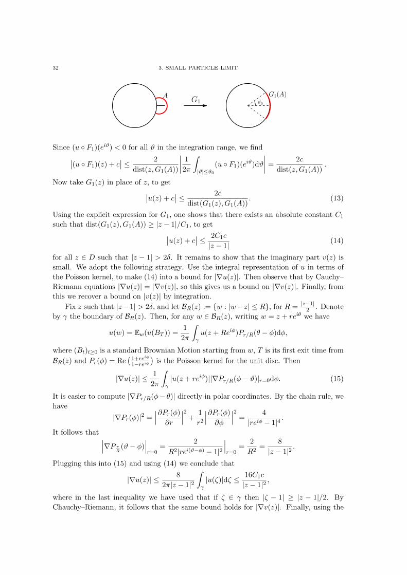
32 3. SMALL PARTICLE LIMIT
AG1 ϑ0
G1(A)
Since (u F1)(eiϑ) < 0 for all ϑ in the integration range, we find∣∣(u F1)(z) + c∣∣ ≤ 2
dist(z,G1(A))
∣∣∣∣ 1
2π
∫|ϑ|≤ϑ0
(u F1)(eiϑ)dϑ
∣∣∣∣ =2c
dist(z,G1(A)).
Now take G1(z) in place of z, to get∣∣u(z) + c∣∣ ≤ 2c
dist(G1(z), G1(A)). (13)
Using the explicit expression for G1, one shows that there exists an absolute constant C1
such that dist(G1(z), G1(A)) ≥ |z − 1|/C1, to get∣∣u(z) + c∣∣ ≤ 2C1c
|z − 1| (14)
for all z ∈ D such that |z − 1| > 2δ. It remains to show that the imaginary part v(z) is
small. We adopt the following strategy. Use the integral representation of u in terms of
the Poisson kernel, to make (14) into a bound for |∇u(z)|. Then observe that by Cauchy–
Riemann equations |∇u(z)| = |∇v(z)|, so this gives us a bound on |∇v(z)|. Finally, from
this we recover a bound on |v(z)| by integration.
Fix z such that |z−1| > 2δ, and let BR(z) := w : |w−z| ≤ R, for R = |z−1|2 . Denote
by γ the boundary of BR(z). Then, for any w ∈ BR(z), writing w = z + reiθ we have
u(w) = Ew(u(BT )) =1
2π
∫γu(z +Reiφ)Pr/R(θ − φ)dφ,
where (Bt)t≥0 is a standard Brownian Motion starting from w, T is its first exit time from
BR(z) and Pr(φ) = Re(
1+reiφ
1−reiφ)
is the Poisson kernel for the unit disc. Then
|∇u(z)| ≤ 1
2π
∫γ|u(z + reiφ)||∇Pr/R(φ− ϑ)|r=0dφ. (15)
It is easier to compute |∇Pr/R(φ− θ)| directly in polar coordinates. By the chain rule, we
have
|∇Pr(φ)|2 =∣∣∣∂Pr(φ)
∂r
∣∣∣2 +1
r2
∣∣∣∂Pr(φ)
∂φ
∣∣∣2 =4
|reiφ − 1|4 .
It follows that ∣∣∣∇P rR
(ϑ− φ)∣∣∣r=0
=2
R2|rei(ϑ−φ) − 1|2∣∣∣r=0
=2
R2=
8
|z − 1|2 .
Plugging this into (15) and using (14) we conclude that
|∇u(z)| ≤ 8
2π|z − 1|2∫γ|u(ζ)|dζ ≤ 16C1c
|z − 1|2 ,
where in the last inequality we have used that if ζ ∈ γ then |ζ − 1| ≥ |z − 1|/2. By
Chauchy–Riemann, it follows that the same bound holds for |∇v(z)|. Finally, using the
1. PRELIMINARY ESTIMATES 33
Fundamental Theorem of Calculus (also known as Gradient Theorem in this setting) we
find
v(z) =
∫ ∞0∇v(z + s(z − 1)) · (z − 1)ds,
from which
|v(z)| ≤∫ ∞
0|∇v(z + s(z − 1))| · |z − 1|ds ≤ 16C1c
|z − 1|
∫ ∞0
1
(1 + s)2ds =
16C1c
|z − 1| .
This, together with (14), concludes the proof.
A similar strategy allows us to prove Corollary 3.1.
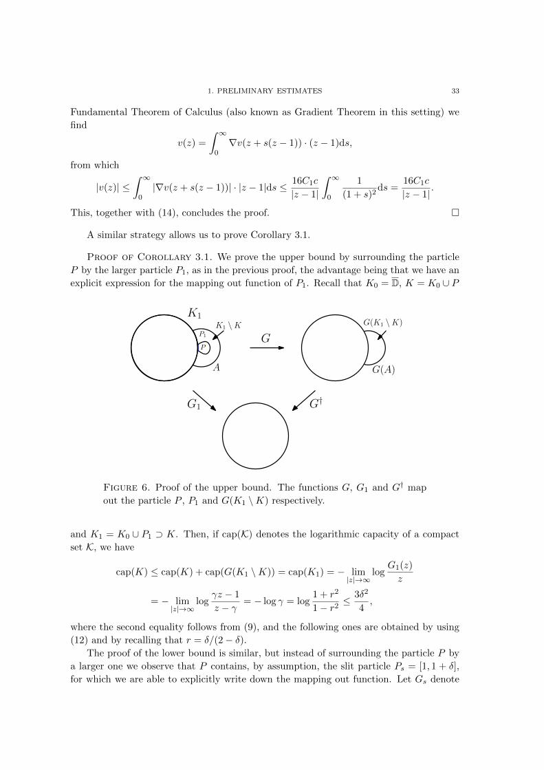
Proof of Corollary 3.1. We prove the upper bound by surrounding the particle
P by the larger particle P1, as in the previous proof, the advantage being that we have an
explicit expression for the mapping out function of P1. Recall that K0 = D, K = K0 ∪ P
G
K1
A
P
G(A)
G(K1 \K)K1 \K
G1 G†
P1
Figure 6. Proof of the upper bound. The functions G, G1 and G† map
out the particle P , P1 and G(K1 \K) respectively.
and K1 = K0 ∪ P1 ⊃ K. Then, if cap(K) denotes the logarithmic capacity of a compact
set K, we have
cap(K) ≤ cap(K) + cap(G(K1 \K)) = cap(K1) = − lim|z|→∞
logG1(z)
z
= − lim|z|→∞
logγz − 1
z − γ = − log γ = log1 + r2
1− r2≤ 3δ2
4,
where the second equality follows from (9), and the following ones are obtained by using
(12) and by recalling that r = δ/(2− δ).The proof of the lower bound is similar, but instead of surrounding the particle P by
a larger one we observe that P contains, by assumption, the slit particle Ps = [1, 1 + δ],
for which we are able to explicitly write down the mapping out function. Let Gs denote
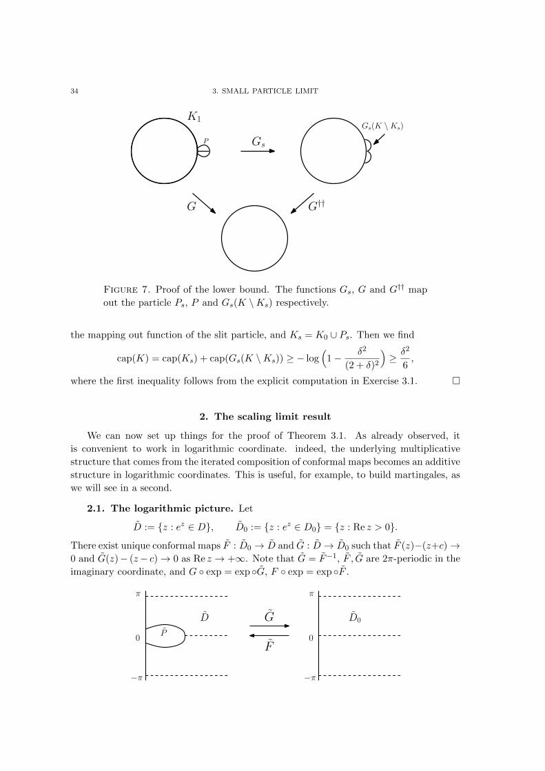
34 3. SMALL PARTICLE LIMIT
Gs
K1
P
Gs(K \Ks)
G G††
Figure 7. Proof of the lower bound. The functions Gs, G and G†† map
out the particle Ps, P and Gs(K \Ks) respectively.
the mapping out function of the slit particle, and Ks = K0 ∪ Ps. Then we find
cap(K) = cap(Ks) + cap(Gs(K \Ks)) ≥ − log(
1− δ2
(2 + δ)2
)≥ δ2
6,
where the first inequality follows from the explicit computation in Exercise 3.1.
2. The scaling limit result
We can now set up things for the proof of Theorem 3.1. As already observed, it
is convenient to work in logarithmic coordinate. indeed, the underlying multiplicative
structure that comes from the iterated composition of conformal maps becomes an additive
structure in logarithmic coordinates. This is useful, for example, to build martingales, as
we will see in a second.
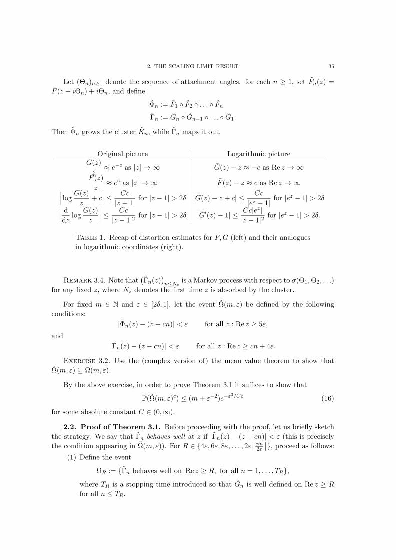
2.1. The logarithmic picture. Let
D := z : ez ∈ D, D0 := z : ez ∈ D0 = z : Re z > 0.There exist unique conformal maps F : D0 → D and G : D → D0 such that F (z)−(z+c)→0 and G(z)− (z− c)→ 0 as Re z → +∞. Note that G = F−1, F , G are 2π-periodic in the
imaginary coordinate, and G exp = exp G, F exp = exp F .
0
π
−π
P
D G
F0
π
−π
D0
2. THE SCALING LIMIT RESULT 35
Let (Θn)n≥1 denote the sequence of attachment angles. for each n ≥ 1, set Fn(z) =
F (z − iΘn) + iΘn, and define
Φn := F1 F2 . . . FnΓn := Gn Gn−1 . . . G1.
Then Φn grows the cluster Kn, while Γn maps it out.
Original picture Logarithmic pictureG(z)
z≈ e−c as |z| → ∞ G(z)− z ≈ −c as Re z →∞
F (z)
z≈ ec as |z| → ∞ F (z)− z ≈ c as Re z →∞∣∣∣ log
G(z)
z+ c∣∣∣ ≤ Cc
|z − 1| for |z − 1| > 2δ |G(z)− z + c| ≤ Cc
|ez − 1| for |ez − 1| > 2δ∣∣∣ d
dzlog
G(z)
z
∣∣∣ ≤ Cc
|z − 1|2 for |z − 1| > 2δ |G′(z)− 1| ≤ Cc|ez||z − 1|2 for |ez − 1| > 2δ.
Table 1. Recap of distortion estimates for F,G (left) and their analogues
in logarithmic coordinates (right).
Remark 3.4. Note that(Γn(z)
)n≤Nz is a Markov process with respect to σ(Θ1,Θ2, . . .)
for any fixed z, where Nz denotes the first time z is absorbed by the cluster.
For fixed m ∈ N and ε ∈ [2δ, 1], let the event Ω(m, ε) be defined by the following
conditions:
|Φn(z)− (z + cn)| < ε for all z : Re z ≥ 5ε,
and
|Γn(z)− (z − cn)| < ε for all z : Re z ≥ cn+ 4ε.
Exercise 3.2. Use the (complex version of) the mean value theorem to show that
Ω(m, ε) ⊆ Ω(m, ε).
By the above exercise, in order to prove Theorem 3.1 it suffices to show that
P(Ω(m, ε)c) ≤ (m+ ε−2)e−ε3/Cc (16)
for some absolute constant C ∈ (0,∞).
2.2. Proof of Theorem 3.1. Before proceeding with the proof, let us briefly sketch
the strategy. We say that Γn behaves well at z if |Γn(z)− (z − cn)| < ε (this is precisely
the condition appearing in Ω(m, ε)). For R ∈ 4ε, 6ε, 8ε, . . . , 2ε⌈cm2ε
⌉, proceed as follows:
(1) Define the event
ΩR := Γn behaves well on Re z ≥ R, for all n = 1, . . . , TR,where TR is a stopping time introduced so that Gn is well defined on Re z ≥ R
for all n ≤ TR.
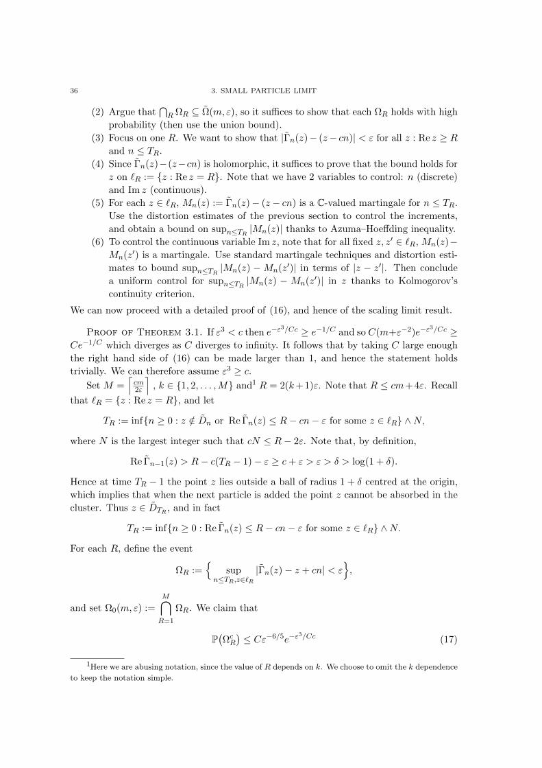
36 3. SMALL PARTICLE LIMIT
(2) Argue that⋂R ΩR ⊆ Ω(m, ε), so it suffices to show that each ΩR holds with high
probability (then use the union bound).
(3) Focus on one R. We want to show that |Γn(z)− (z− cn)| < ε for all z : Re z ≥ Rand n ≤ TR.
(4) Since Γn(z)−(z−cn) is holomorphic, it suffices to prove that the bound holds for
z on `R := z : Re z = R. Note that we have 2 variables to control: n (discrete)
and Im z (continuous).
(5) For each z ∈ `R, Mn(z) := Γn(z)− (z − cn) is a C-valued martingale for n ≤ TR.
Use the distortion estimates of the previous section to control the increments,
and obtain a bound on supn≤TR |Mn(z)| thanks to Azuma–Hoeffding inequality.
(6) To control the continuous variable Im z, note that for all fixed z, z′ ∈ `R, Mn(z)−Mn(z′) is a martingale. Use standard martingale techniques and distortion esti-
mates to bound supn≤TR |Mn(z) −Mn(z′)| in terms of |z − z′|. Then conclude
a uniform control for supn≤TR |Mn(z) − Mn(z′)| in z thanks to Kolmogorov’s
continuity criterion.
We can now proceed with a detailed proof of (16), and hence of the scaling limit result.
Proof of Theorem 3.1. If ε3 < c then e−ε3/Cc ≥ e−1/C and so C(m+ε−2)e−ε
3/Cc ≥Ce−1/C which diverges as C diverges to infinity. It follows that by taking C large enough
the right hand side of (16) can be made larger than 1, and hence the statement holds
trivially. We can therefore assume ε3 ≥ c.Set M =
⌈cm2ε
⌉, k ∈ 1, 2, . . . ,M and1 R = 2(k+1)ε. Note that R ≤ cm+4ε. Recall
that `R = z : Re z = R, and let
TR := infn ≥ 0 : z /∈ Dn or Re Γn(z) ≤ R− cn− ε for some z ∈ `R ∧N,
where N is the largest integer such that cN ≤ R− 2ε. Note that, by definition,
Re Γn−1(z) > R− c(TR − 1)− ε ≥ c+ ε > ε > δ > log(1 + δ).
Hence at time TR − 1 the point z lies outside a ball of radius 1 + δ centred at the origin,
which implies that when the next particle is added the point z cannot be absorbed in the
cluster. Thus z ∈ DTR , and in fact
TR := infn ≥ 0 : Re Γn(z) ≤ R− cn− ε for some z ∈ `R ∧N.
For each R, define the event
ΩR :=
supn≤TR,z∈`R
|Γn(z)− z + cn| < ε,
and set Ω0(m, ε) :=M⋂R=1
ΩR. We claim that
P(ΩcR
)≤ Cε−6/5e−ε
3/Cc (17)
1Here we are abusing notation, since the value of R depends on k. We choose to omit the k dependence
to keep the notation simple.

2. THE SCALING LIMIT RESULT 37
(note that the upper bound does not depend on R). Assuming this, we find
P(Ω0(m, ε)c
)≤
M∑k=1
P(Ωc
2(k+1)ε
)≤MCε−6/5e−ε
3/Cc
≤(cm
2ε+ 1)Cε−6/5e−ε
3/Cc ≤ C(m+ ε−2)e−ε3/Cc.
The theorem will then follow provided we can show that Ω0(m, ε) ⊆ Ω(m, ε). To see
this, assume that Ω0(m, ε) holds. Then ΩR holds for all R = 1, . . . ,M . Take z such that
Re z ≥ 4ε+ cn. Then we can choose R so that Re z ≥ R, and so by the definition of ΩR
supn≤TR,z∈`R
|Γn(z)− z + cn| = supn≤TR,Re z≥R
|Γn(z)− z + cn| < ε,
where the first equality holds by the maximum principle (cf. Theorem 1.6). Moreover,
since on ΩR we have |ΓTR(z) − z + cTR| < ε for all z ∈ `R, it must be TR = N . It
follows that the second condition defining Ω(m, ε) holds. For the first one, simply map
everything back via Γn: we show that z : Re z ≥ 5ε gets mapped to z : Re z > cn+ εby Φn. Indeed, if z ∈ `R then Re Γn(z) < 5ε, so the curve Γn(`R) lies to the left of
z : Re z ≥ 5ε. Thus the image of z : Re z ≥ 5ε must lie to the right of `R. More
precisely, take R maximum so that R ≤ m + 4ε. Then if z ∈ `R, on the event ΩR we
have that |Γn(z) − z + cn| < ε, which implies Re Γn(z) < ε + Re(z) − cn ≤ 5ε. Thus if
Re z ≥ 5ε, Φn(z) > R, from which |Γn(Φn(z))− Φn(z) + cn| = |Φn(z)− z − cn| < ε. This
shows that Ω0(m, ε) ⊆ Ω(m, ε).
Φn
Γn
`5εΦn(`5ε)
`RΓn(`R)
In order to conclude the proof of the theorem now we only have to show that (17)
holds for each fixed R ∈ 1, . . . ,M. As mentioned, we do so via martingale techniques.
For z ∈ Dn, let
Mn(z) := Γn(z)− z + cn.
Then
Mn+1(z)−Mn(z) = Γn+1(z)− Γn(z) + c
= G(Γn(z)− iΘn+1)− (Γn(z)− iΘn+1) + c
= G0(Γn(z)− iΘn+1) + c,
38 3. SMALL PARTICLE LIMIT
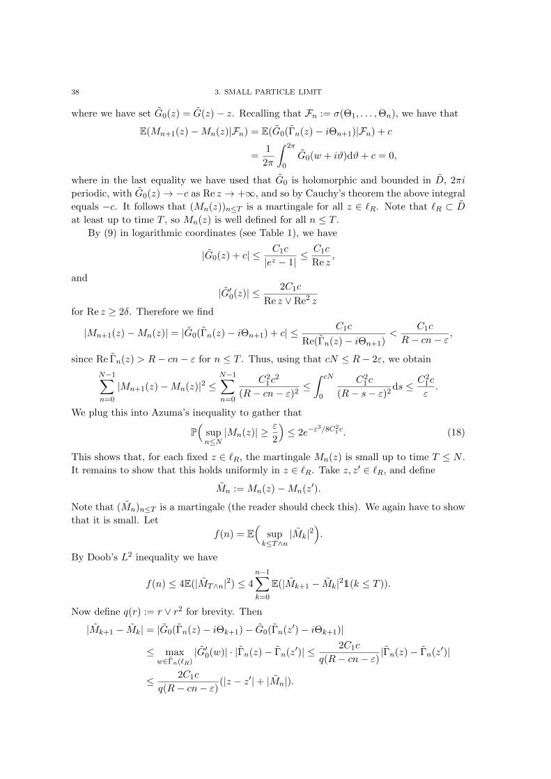
where we have set G0(z) = G(z)− z. Recalling that Fn := σ(Θ1, . . . ,Θn), we have that
E(Mn+1(z)−Mn(z)|Fn) = E(G0(Γn(z)− iΘn+1)|Fn) + c
=1
2π
∫ 2π
0G0(w + iϑ)dϑ+ c = 0,
where in the last equality we have used that G0 is holomorphic and bounded in D, 2πi
periodic, with G0(z)→ −c as Re z → +∞, and so by Cauchy’s theorem the above integral
equals −c. It follows that (Mn(z))n≤T is a martingale for all z ∈ `R. Note that `R ⊂ D
at least up to time T , so Mn(z) is well defined for all n ≤ T .
By (9) in logarithmic coordinates (see Table 1), we have
|G0(z) + c| ≤ C1c
|ez − 1| ≤C1c
Re z,
and
|G′0(z)| ≤ 2C1c
Re z ∨ Re2 zfor Re z ≥ 2δ. Therefore we find
|Mn+1(z)−Mn(z)| = |G0(Γn(z)− iΘn+1) + c| ≤ C1c
Re(Γn(z)− iΘn+1)<
C1c
R− cn− ε,
since Re Γn(z) > R− cn− ε for n ≤ T . Thus, using that cN ≤ R− 2ε, we obtain
N−1∑n=0
|Mn+1(z)−Mn(z)|2 ≤N−1∑n=0
C21c
2
(R− cn− ε)2≤∫ cN
0
C21c
(R− s− ε)2ds ≤ C2
1c
ε.
We plug this into Azuma’s inequality to gather that
P(
supn≤N|Mn(z)| ≥ ε
2
)≤ 2e−ε
3/8C21c. (18)
This shows that, for each fixed z ∈ `R, the martingale Mn(z) is small up to time T ≤ N .
It remains to show that this holds uniformly in z ∈ `R. Take z, z′ ∈ `R, and define
Mn := Mn(z)−Mn(z′).
Note that (Mn)n≤T is a martingale (the reader should check this). We again have to show
that it is small. Let
f(n) = E(
supk≤T∧n
|Mk|2).
By Doob’s L2 inequality we have
f(n) ≤ 4E(|MT∧n|2) ≤ 4n−1∑k=0
E(|Mk+1 − Mk|21(k ≤ T )).
Now define q(r) := r ∨ r2 for brevity. Then
|Mk+1 − Mk| = |G0(Γn(z)− iΘk+1)− G0(Γn(z′)− iΘk+1)|
≤ maxw∈Γn(`R)
|G′0(w)| · |Γn(z)− Γn(z′)| ≤ 2C1c
q(R− cn− ε) |Γn(z)− Γn(z′)|
≤ 2C1c
q(R− cn− ε)(|z − z′|+ |Mn|).

2. THE SCALING LIMIT RESULT 39
It follows that
E(|Mk+1 − Mk|21(k ≤ T )) ≤ 4
[2C1c
q(R− cn− ε)
]2
E((|z − z′|+ |Mn|)2)
≤ 8
[2C1c
q(R− cn− ε)
]2
(|z − z′|2 + f(k)),
and hence
f(n) ≤ 32C21c
2n−1∑k=0
|z − z′|2 + f(k)
(q(R− ck − ε))2.
It is left to the reader as an exercise to show that this implies
f(n) = E(
supk≤T∧n
|Mk|2)≤ C2
c
ε3|z − z′|2
for some absolute constant C2 (hint: use the discrete version of Gronwall’s inequality).
Kolmogorov’s continuity theorem, then, yields the existence of a random variable M with
E(M 2) ≤ C2cε3
such that
supk≤T|Mk(z)−Mk(z
′)| ≤M |z − z′|1/3
for all z, z′ ∈ `R, almost surely. Note that by periodicity |z − z′| ≤ π. On the other hand,
the above estimate is good when z and z′ are close. To take this into account, we introduce
L ≥ 2 and observe that
P(
supk≤T|Mk(z)−Mk(z
′)| ≥ ε
2for some z, z′ ∈ `R with |z − z′| ≤ π
L
)≤ P
(M |z − z′|1/3 ≥ ε
2for some z, z′ ∈ `R with |z − z′| ≤ π
L
)≤ 4
ε2
(πL
)2/3E(M 2) ≤ 4C2c
ε5
(πL
)2/3.
It follows that
P(ΩcR) = P
(sup
z∈`R,n≤T|Mn(z)| > ε
)= P
(∃z ∈ `R : sup
k≤T|Mk(z)| > ε
)≤ P
(∃z ∈ `R : sup
k≤T|Mk(z)−Mk(z
′)|+ supk≤T|Mk(z
′)| > ε for some |z − z′| ≤ π/L)
≤ P(
supk≤T|Mk(z)−Mk(z
′)| > ε
2for some z, z′ ∈ `R, |z − z′| ≤ π/L
)+ P
(supk≤T|Mk(z
′)| > ε
2
)≤ 4C2c
ε5
(πL
)2/3+ Le−ε
3/8C21c,
where the last inequality follows from (18) using that L ≥ 2. It is now left to the reader
to optimise over L, to gather that
P(ΩcR) ≤ Cε−6/5e−ε
3/Cc
for some absolute constant C > 0. This proves Claim 17, thus concluding the proof of
Theorem 3.1.
40 3. SMALL PARTICLE LIMIT
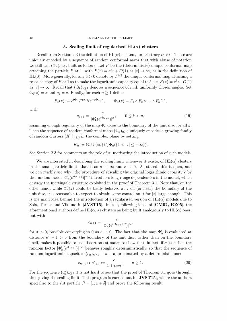
3. Scaling limit of regularised HL(α) clusters
Recall from Section 2.3 the definition of HL(α) clusters, for arbitrary α > 0. These are
uniquely encoded by a sequence of random conformal maps that with abuse of notation
we still call (Φn)n≥1, built as follows. Let F be the (deterministic) unique conformal map
attaching the particle P at 1, with F (z) = ecz +O(1) as |z| → ∞, as in the definition of
HL(0). More generally, for any c > 0 denote by F (c) the unique conformal map attaching a
rescaled copy of P at 1 so to make the logarithmic capacity equal to c, i.e. F (z) = ecz+O(1)
as |z| → ∞. Recall that (Θk)k≥1 denotes a sequence of i.i.d. uniformly chosen angles. Set
Φ0(z) = z and c1 = c. Finally, for each n ≥ 1 define
Fn(z) := eiΘnF (cn)(e−iΘnz), Φn(z) = F1 F2 . . . Fn(z),
with
ck+1 =c
|Φ′k(eiΘk+1)|α, 0 ≤ k < n, (19)
assuming enough regularity of the map Φk close to the boundary of the unit disc for all k.
Then the sequence of random conformal maps (Φn)n≥0 uniquely encodes a growing family
of random clusters (Kn)n≥0 in the complex plane by setting
Kn := (C ∪ ∞) \ Φn(1 < |z| ≤ +∞).
See Section 2.3 for comments on the role of α, motivating the introduction of such models.
We are interested in describing the scaling limit, whenever it exists, of HL(α) clusters
in the small particle limit, that is as n → ∞ and c → 0. As stated, this is open, and
we can readily see why: the procedure of rescaling the original logarithmic capacity c by
the random factor |Φ′n(eiΘn+1)|−α introduces long range dependencies in the model, which
destroy the martingale structure exploited in the proof of Theorem 3.1. Note that, on the
other hand, while Φ′n(z) could be badly behaved at z on (or near) the boundary of the
unit disc, it is reasonable to expect to obtain some control on it for |z| large enough. This
is the main idea behind the introduction of a regularised version of HL(α) models due to
Sola, Turner and Viklund in [JVST15]. Indeed, following ideas of [CM02, RZ05], the
aforementioned authors define HL(α, σ) clusters as being built analogously to HL(α) ones,
but with
cn+1 =c
|Φ′n(eiΘn+1+σ)|α,
for σ > 0, possible converging to 0 as c → 0. The fact that the map Φ′n is evaluated at
distance eσ − 1 > σ from the boundary of the unit disc, rather than on the boundary
itself, makes it possible to use distortion estimates to show that, in fact, if σ c then the
random factor |Φ′n(eiΘn+1)|−α behaves roughly deterministically, so that the sequence of
random logarithmic capacities (cn)n≥1 is well approximated by a deterministic one:
cn+1 ≈ c∗n+1 :=c
1 + αcn, n ≥ 1. (20)
For the sequence (c∗n)n≥1 it is not hard to see that the proof of Theorem 3.1 goes through,
thus giving the scaling limit. This program is carried out in [JVST15], where the authors
specialise to the slit particle P = [1, 1 + δ] and prove the following result.

3. SCALING LIMIT OF REGULARISED HL(α) CLUSTERS 41
Theorem 3.2 ([JVST15]). Let α > 0 be fixed, and let (Φn)n≥0 denote the sequence
of random conformal maps growing HL(α, σ) clusters in the complex plane. Assume that
σ (log c−1)−1/2 as c → 0. Then, in the limit as n → ∞, c → 0 and nc → t ∈ (0,∞)
the map Φn converges in distribution to the deterministic map Ψt(z) := (1 +αt)1/αz, with
respect to uniform convergence on compact sets bounded away from the unit disc.
Note that as α 0 one recovers the scaling limit z 7→ etz of HL(0) clusters.
While we do not try to survey the proof of this result, we next briefly comment on
the form of the approximating sequence (c∗n)n≥1 defined in (20), following the discussion
in [JVST15]. To see how this sequence arises, let us look at very large values of σ. By
the chain rule we have
|Φ′n(z)| =n∏k=1
|F ′k(Φn−k(z))|, z = eiΘn+1+σ.
Now if σ 1, formally σ = +∞, we have
|F ′k(Φn−k(z))| = |F ′(∞)| = eck = exp
c
|Φ′k−1(eiΘk+1+σ)|α,
from which
|Φ′n(z)|−α =n∏k=1
exp
− α c
|Φ′k−1(z)|α. (21)
Setting q(k) = |Φ′k(z)|−α for brevity, we have
q(n) = exp− αc
n−1∑k=1
q(k).
It only remains to solve the recursion. We find
q(k)− q(k − 1)
q(k − 1)= eαcq(k−1) − 1 = −αcq(k − 1) +O(c2q(k − 1)2)
= −αcq(k − 1) +O(c2)
(22)
where we have used that c 1 to Taylor expand the exponential, and the fact that
q(k− 1) ≤ 1, which follows from (21). Dividing further both sides of (22) by q(k− 1) and
summing over k we findn∑k=1
q(k)− q(k − 1)
q(k − 1)2≈∫ n
0
q′(x)
q(x)2dx = 1− 1
q(n),
where q(x) is any differentiable interpolation of q(n). Thus we end up with 1 − 1q(n) =
−αcn+ nO(c2) which, rearranging and using that nc→ t, gives
q(n) =1
1 + αcn+O(c).
In conclusion, we have shown that for σ 1
cn+1 = cq(n) =c
1 + αcn+O(c2),
which justifies (20).

CHAPTER 4
Fluctuations
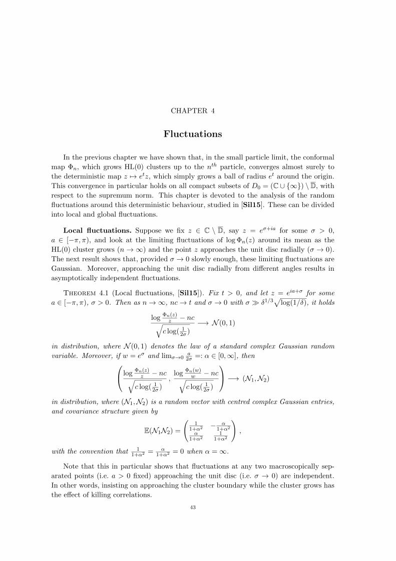
In the previous chapter we have shown that, in the small particle limit, the conformal
map Φn, which grows HL(0) clusters up to the nth particle, converges almost surely to
the deterministic map z 7→ etz, which simply grows a ball of radius et around the origin.
This convergence in particular holds on all compact subsets of D0 = (C ∪ ∞) \ D, with
respect to the supremum norm. This chapter is devoted to the analysis of the random
fluctuations around this deterministic behaviour, studied in [Sil15]. These can be divided
into local and global fluctuations.
Local fluctuations. Suppose we fix z ∈ C \ D, say z = eσ+ia for some σ > 0,
a ∈ [−π, π), and look at the limiting fluctuations of log Φn(z) around its mean as the
HL(0) cluster grows (n→∞) and the point z approaches the unit disc radially (σ → 0).
The next result shows that, provided σ → 0 slowly enough, these limiting fluctuations are
Gaussian. Moreover, approaching the unit disc radially from different angles results in
asymptotically independent fluctuations.
Theorem 4.1 (Local fluctuations, [Sil15]). Fix t > 0, and let z = eia+σ for some
a ∈ [−π, π), σ > 0. Then as n→∞, nc→ t and σ → 0 with σ δ1/3√
log(1/δ), it holds
log Φn(z)z − nc√
c log( 12σ )
−→ N (0, 1)
in distribution, where N (0, 1) denotes the law of a standard complex Gaussian random
variable. Moreover, if w = eσ and limσ→0a
2σ =: α ∈ [0,∞], then log Φn(z)z − nc√
c log( 12σ )
,log Φn(w)
w − nc√c log( 1
2σ )
−→ (N1,N2)
in distribution, where (N1,N2) is a random vector with centred complex Gaussian entries,
and covariance structure given by
E(N1N2) =
(1
1+α2 − α1+α2
α1+α2
11+α2
),
with the convention that 11+α2 = α
1+α2 = 0 when α =∞.
Note that this in particular shows that fluctuations at any two macroscopically sep-
arated points (i.e. a > 0 fixed) approaching the unit disc (i.e. σ → 0) are independent.
In other words, insisting on approaching the cluster boundary while the cluster grows has
the effect of killing correlations.
43
44 4. FLUCTUATIONS
Global fluctuations. At the price of keeping z away from the unit disc while the
cluster grows, we see that the fluctuations of log Φn become rather well behaved. Indeed,
by the same techniques that allow us to prove the local fluctuations result, we can show
(cf. Theorem 4.3) that, for any fixed z ∈ C \ D, these fluctuations are again centred
Gaussian, with variance now depending on |z| and t. Moreover, the correlation structure
is sufficiently well behaved to enable us to prove a functional central limit theorem for
log Φn when restricted to any circle of the form rT := z : |z| = r, r > 1 (cf. Theorem
4.5). Finally, we push our analysis forward to obtain limiting fluctuations of log Φn viewed
as a random variable in the space of holomorphic functions on C \ D. Our main result is
the following.
Theorem 4.2 (Global fluctuations, [Sil15]). Let H denote the space of holomorphic
functions on |z| > 1, and for n ≥ 1 set
Fn(z) =1√c
(log
Φn(z)
z− nc
).
Then there exists a random variable F in H such that Fn → F in distribution as n→∞,
with respect to the supremum norm on compacts of (C ∪ ∞) \ D. Moreover, F can be
obtained as the holomorphic extension of its boundary values on |z| = 1 to the outer
unit disc |z| > 1. These boundary values are given by a distribution–valued Gaussian
random variable W, formally defined in Fourier space by
W(ϑ) =∑
k∈Z\0
√1− e−2|k|t
|k|(Ak + iBk√
2
) eikϑ√2π
,
for (Ak)k, (Bk)k independent collections of i.i.d. N (0, 1) random variables.
This provides an explicit construction of the limiting Gaussian holomorphic field Fand, perhaps more interestingly, of its boundary values.
Remark 4.1. Note that, setting formally t =∞, we have
W∞(ϑ) =∑
k∈Z\0
|k|−1/2(Ak + iBk√
2
) eikϑ√2π
,
This is (the complex version of) a well-known Fractional Gaussian Field (FGF) on the
unit circle T, and it can be realised as W∞ = (−∆)−1/4W , where ∆ denotes the Laplace
operator1, and W is white noise on T. Fractional Gaussian Fields can be studied in greater
generality: we refer the interested reader to [DRSV14, LSSW14] and references therein.
Let ∆ and W denote the Laplace operator and White Noise on the d–dimensional torus
respectively, for any d ≥ 1. Then (−∆)−s/2W defines an FGF for any s ∈ R. This is
a (random) continuous function if s > d/2, and otherwise it takes values in the space
of distributions. Moreover, at the critical parameter s = d/2 it defines a Log–correlated
Gaussian Field (LGF), which coincides with the Gaussian Free Field when d = 2. By
taking d = 1, we see that W∞ coincides with the critical LGF on the 1–dimensional torus
T, which is also the restriction of a 2–dimensional Gaussian Free Field to T. It is possible
to show that the law of W for any finite t is absolutely continuous with respect to the one
1Recall that the eigenvalues of the operator −∆ on T are given by k2 : k ≥ 1.

1. PRELIMINARY ESTIMATES 45
of W∞, and in fact this can be made precise by constructing W as a stochastic process in
the space of distributions on T, which converges to W∞ as t→∞. We do not survey this
here, and refer the interested reader to [Sil15].
The rest of this chapter is devoted to the proof of Theorem 4.2, which is based on
martingale techniques. We proceed in steps. In Section 1 we collect some preliminary es-
timates for the basic conformal maps F,G, as in the previous chapter. We then introduce in
Section 2 our main tools, namely two sequences of backwards martingale difference arrays
(27), and prove Theorem 4.3 on pointwise fluctuations. This result is then generalised in
Sections 3-3.2 to obtain a central limit theorem for the sequence z 7→ log Φn(z)/z, viewed
as a random variable in the space of holomorphic functions on |z| > 1, thus completing
the proof.
1. Preliminary estimates
Recall that in Proposition 3.1 we showed that log G(z)z ≈ −c, and this approximation
gets better as z moves away from the cluster boundary. In order to study fluctuations,
on the other hand, a first order approximation turns out not to be enough. The following
result improves on Proposition 3.1.
Proposition 4.1. There exists an absolute constant C > 0 such that, for all z ∈ D:
|z − 1| > 2δ, it holds: ∣∣∣∣ log(G(z)
z
)+ c
z + 1
z − 1
∣∣∣∣ ≤ Cc3/2|z||z − 1|2 . (23)
The proof of the above result is spelled out in [Sil15], and it follows the one of Propo-
sition 3.1 with minor modifications. We combine Propositions 3.1 and 4.1 to obtain cor-
responding estimates for the function F , which are collected below.
Corollary 4.1. There exists a constant C > 0 such that, for all z ∈ D0 with |F (z)−1| > 2δ, it holds:
|F (z)− ecz| ≤ Cc|z||z| − 1
,
∣∣∣∣ log(F (z)
z
)− c z + 1
z − 1
∣∣∣∣ ≤ Cc3/2|z|2(|z| − 1)3
.
Proof. For the first inequality, note that (9) readily implies that
|G(z)− e−cz| ≤ Cc|z||z − 1| (24)
for all z ∈ D : |z − 1| > δ, and δ small enough. Therefore, by setting w = F (z) and using
(P1)-(P2), we obtain
|F (z)− ecz| = ec|G(w)− e−cw| ≤ Cc|w||w − 1| ≤
C ′c|z||z| − 1
, (25)
for all z ∈ D0 such that |F (z)− 1| > 2δ and δ small enough, as claimed.

46 4. FLUCTUATIONS
For the second inequality, note that, since |F (z)− 1| > 2δ by assumption, we can use
(23) to get∣∣∣∣ logF (z)
z− c z + 1
z − 1
∣∣∣∣ ≤ ∣∣∣∣ logG(w)
w+ c
w + 1
w − 1
∣∣∣∣+ 2c
∣∣∣∣ 1
w − 1− 1
G(w)− 1
∣∣∣∣≤ Cc3/2|w||w − 1|2 +
2c|G(w)− w||w − 1||G(w)− 1| ≤
Cc3/2|z|(|z| − 1)2
+2c|G(w)− w|
(|z| − 1)2.
Moreover, it follows from (25) that
|G(w)− w| ≤ |F (z)− ecz|+ (1− e−c)|w| ≤ Cc|z||z| − 1
+ Cc|z| ≤ Cc|z|2|z| − 1
for c small enough. Putting all together, we end up with∣∣∣∣ logF (z)
z− c z + 1
z − 1
∣∣∣∣ ≤ Cc3/2|z|(|z| − 1)2
(1 +
√c|z|
|z| − 1
)≤ 2Cc3/2|z|2
(|z| − 1)3
for c small enough, as claimed.
2. Pointwise fluctuations
In this section we prove that, fixed t ≥ 0 and z ∈ C \ D, the fluctuations of log Φn(z)
around its mean are given by a complex Gaussian random variable, whose variance is
independent of Arg(z).
Theorem 4.3. Pick a ∈ [−π, π), σ > 0, and let z = eia+σ. Define
v2t (σ) := log
1− e−2(σ+t)
1− e−2σ,
and let Fσ(t, eia) be a complex Gaussian random variable with i.i.d. real and imaginary
part, distributed according to N (0, v2t (σ)). Then it holds:
1√c
(log
Φn(z)
z− nc
)−→ Fσ(eia)
in distribution as n→∞, c→ 0 and nc→ t.
We prove Theorem 4.3 for σ ≤ 1, which we assume without further notice. This entails
no loss of generality, as it will become clear, and it has the advantage of slightly simplifying
the notation.
Our main tool for the proof of Theorem 4.3 consists of two sequences of backwards
martingale difference arrays, that we now define. Note that∣∣Φn(z)
z
∣∣ > 1 for all z ∈ D0, so
log Φn(z)z defines a holomorphic function on D0. For σ > 0 and a ∈ [−π, π) as in Theorem
4.3, then, we find:
logΦn(eia+σ)
eia+σ=
n∑k=1
logFk Fk+1 · · · Fn(eia+σ)
Fk+1 · · · Fn(eia+σ)=
n∑k=1
logF (e−iΘkZσk,n(a))
e−iΘkZσk,n(a),
2. POINTWISE FLUCTUATIONS 47
where Zσk,n(a) := Fk+1 · · · Fn(eia+σ). Moreover, if Fk,n := σ(Θk,Θk+1 . . .Θn), then
E(
logF (e−iΘkZσk,n(a))
e−iΘkZσk,n(a)
∣∣∣∣Fk+1,n
)=
1
2π
∫ π
−πlog
F (e−iϑZσk,n(a))
e−iϑZσk,n(a)dϑ = lim
|z|→∞log
F (z)
z= c .
(26)
We therefore set
Xσk,n(a) =
1√c
(log
∣∣∣∣F (e−iΘkZσk,n(a))
e−iΘkZσk,n(a)
∣∣∣∣− c),Y σk,n(a) =
1√c
Arg
(F (e−iΘkZσk,n(a))
e−iΘkZσk,n(a)
),
(27)
where Arg(z) ∈ [−π, π). The above computation then shows that (Xσk,n(a))k≤n and
(Y σk,n(a))k≤n form sequences of backwards martingale arrays with respect to the same
filtration (Fk,n)k≤n (see [Bil95], Section 35 for the definition of martingale arrays). More-
over,n∑k=1
(Xσk,n(a) + i Y σ
k,n(a))
=1√c
(log
Φn(eia+σ)
eia+σ− nc
).
Remark 4.2. We identify C with R2 throughout, and often refer to complex random
variables as random vectors and vice versa, depending on which point of view we seek to
emphasize.
The following result appears in [McL74], Corollary 2.8, as a Central Limit Theorem
for (forward) martingale difference arrays (see also [Bil95], Theorem 35.12). It is straight-
forward to adapt the proof to backwards martingale difference arrays, so that we have the
following.
Theorem 4.4. Let (Xk,n)1≤k≤n be a backwards martingale difference array with respect
to Fk,n = σ(Xk,n . . .Xn,n). Let Sk,n =∑n
j=k Xj,n. Assume that:
(I) for all η > 0,
n∑k=1
X 2k,n1(|Xk,n| > η)→ 0 in probability as n→∞,
(II)
n∑k=1
X 2k,n → s2 in probability as n→∞, for some s2 > 0.
Then S1,n converges in distribution to N (0, s2).
Note that the above theorem is concerned with scalar random variables, while we have
2–dimensional vectors. In order to reduce to the scalar case, recall that by the Cramer–
Wold Theorem (cf. [Dur10], Theorem 3.9.5) it suffices to prove convergence in distribution
of all linear combinations of the vector entries. To this end, pick any α, β ∈ R, and note
that by linearity(αXσ
k,n(a)+βY σk,n(a)
)k≤n is again a backwards martingale difference array
with respect to the filtration (Fk,n)k≤n. We are going to apply Theorem 4.4 to this linear
combination. To this end, we collect here some estimates for (Xσk,n(a)) and (Y σ
k,n(a)).
Since a and σ are fixed, we omit them from the notation throughout this section.
Lemma 4.1. There exists a constant C > 0 such that, for c small enough, it holds
|Xk,n| ≤ C/√c, |Yk,n| ≤ C/
√c for all n ≥ 1, k ≤ n.
48 4. FLUCTUATIONS
Proof. It follows from (P1) that log∣∣F (e−iΘkZk,n)
e−iΘkZk,n
∣∣ > 0, from which Xk,n > −√c.Moreover, (P2) gives |Xk,n| ≤ C/
√c+√c ≤ 2C/
√c for some constant C > 0 and c small
enough. Finally, since Arg(F (e−iΘkZk,n)
e−iΘkZk,n
)∈ [−π, π), we have |Yk,n| ≤ π/
√c.
Much better estimates can be obtained by restricting to the good event, Ω(m, ε) of
Theorem 3.1, on which for all n ≤ m it holds
|e−cnΦn(z)− z| < εe6ε for all z : |z| ≥ e5ε,
and
|Γn(z)− e−cnz| < εe5ε for all z : |z| ≥ ecn+4ε.
We take m = bδ−6c and ε = δ2/3 log(1/δ) throughout without further notice, so that2
ε δ, m n and P(Ω(m, ε)c) decays faster than any polynomial in δ.
Lemma 4.2. Assume that σ δ as δ → 0. Then there exists a constant C(t) > 0 such
that, for n large enough, on the good event Ω(m, ε) it holds
maxk≤n
|Xk,n| ∨ |Yk,n|
≤ C(t)
√c
σ. (28)
Proof. For any k ≤ n we have
max|Xk,n|; |Yk,n|
≤ 1√
c
(∣∣ logF (e−iΘkZk,n)− log(e−iΘkZk,n)∣∣+ c
)≤ 1√
c
[(sup|ξ|≥eσ
1
|ξ|)·∣∣F (e−iΘkZk,n)− e−iΘkZk,n
∣∣+ c
],
where the last inequality follows from the mean values theorem, and the fact that |F (e−iΘkZk,n)| >|e−iΘkZk,n| > eσ almost surely by (P1). Now note that |F (e−iΘkZk,n)− 1| > |Zk,n| − 1 ≥σ 2δ, so by Corollary 4.1 we have
|F (z)− z| ≤ |F (z)− ecz|+ (ec − 1)|z| ≤ Cc|z||z| − 1
+ 2c|z| ≤ 2Cc|z|2|z| − 1
(29)
for z = e−iΘkZk,n. Moreover, since we are on Ω(m, ε), there exists a constant C(t)
depending only on t such that eσ < |Zk,n| ≤ C(t). This, together with (29), yields
maxk≤n
|Xk,n| ∨ |Yk,n|
≤ 1√
c
(2Cc|Zk,n|2|Zk,n| − 1
+ c
)≤ C(t)
√c
eσ − 1+√c ≤ 2C(t) ·
√c
σ
as claimed.
We now make use of the above bounds to prove that the backwards martingale dif-
ference array (Xk,n)k≤n, with Xk,n := αXk,n + βYk,n, satisfies Assumptions (I)-(II) of
Theorem 4.4. In doing so, we provide an explicit formula for the limiting variance.
Lemma 4.3. Assume that σ δ as δ → 0. Then for all η > 0 it holdsn∑k=1
X 2k,n1(|Xk,n| > η)→ 0
in probability as n→∞.
2If a, b→ 0 (respectively a, b→∞) write a b to mean lima,b→0ba
= 0 (respectively lima,b→∞ba
= 0).
2. POINTWISE FLUCTUATIONS 49
Proof. For any ε > 0 we have:
P( n∑k=1
X 2k,n1(|Xk,n| > η) > ε
)≤ P
(max
1≤k≤n|Xk,n| > η
)≤ 1
ηE(
max1≤k≤n
|Xk,n|)
=1
ηE(
max1≤k≤n
|Xk,n| ; Ω(m, ε)c)
+1
ηE(
max1≤k≤n
|Xk,n| ; Ω(m, ε)
).
The fact that the first term in the r.h.s. converges to zero as n→∞ follows from Lemma
4.1 and Theorem 3.1, while convergence to zero of the second term is a straightforward
consequence of Lemma 4.2.
We now concentrate on Assumption (II). The first step consists in replacing condition
(II) with a more convenient one, involving conditional second moments. The following
result shows that, provided σ is large enough with respect to c, this is allowed.
Lemma 4.4. Assume limδ→0
√δσ = 0, and that
n∑k=1
E(X 2k,n|Fk+1,n) → s2 in probability
as n→∞ for some s2 > 0. Then alson∑k=1
X 2k,n → s2 in probability as n→∞.
Proof. Let Mk,n := X 2k,n − E(X 2
k,n|Fk+1,n). It is readily checked that (Mk,n)k≤n is
a backwards martingale difference array with respect to the filtration (Fk,n)k≤n. We aim
to show that for any η > 0 it holds P(∣∣∣ n∑
k=1
Mk,n
∣∣∣ > η)→ 0 as n→∞. Indeed,
P(∣∣∣ n∑
k=1
Mk,n
∣∣∣ > η)≤ 1
η2E([ n∑
k=1
Mk,n
]2)=
1
η2
n∑k=1
E(M2k,n)
(∗)≤ 1
η2
n∑k=1
E(X 4k,n)
=1
η2
n∑k=1
E(X 4k,n;E(m, ε)c) +
1
η2
n∑k=1
E(X 4k,n;E(m, ε)) .
Above, (∗) follows from the general inequality E((X − E(X))2) ≤ E(X2), which we apply
to each term with respect to E( · |Fk,n). The fact that both terms in the r.h.s. converge
to zero as n→∞ is now a consequence of the bounds for |Xk,n| and |Yk,n|, and hence for
|Xk,n|, obtained in Lemmas 4.1–4.2.
In light of the above result, it remains to compute the limit in probability of
n∑k=1
E(X 2k,n|Fk+1,n) = α2
n∑k=1
E(X2k,n|Fk+1,n) + β2
n∑k=1
E(Y 2k,n|Fk+1,n)
+ 2αβn∑k=1
E(Xk,nYk,n|Fk+1,n) ,
and prove that it coincides with (α2 + β2)v2t (σ), where v2
t (σ) is the limiting variance
introduced in Theorem 4.3. The following result shows that, in fact, it suffices to compute
the limit of the first term in the r.h.s. above.

50 4. FLUCTUATIONS
Proposition 4.2. Almost surely, it holds
E(X2k,n|Fk+1,n) = E(Y 2
k,n|Fk+1,n)
E(Xk,nYk,n|Fk+1,n) = 0
for all k ≤ n.
Proof. All equalities in this proof are intended to hold almost surely. Introduce the
holomorphic function f(z) := 1√c
(log F (z)
z − c)
defined for |z| > 1, so that[f(e−iΘkZk,n)
]2= X2
k,n − Y 2k,n + 2iXk,nYk,n .
Taking conditional expectations both sides, we find
1
2π
∫ π
−π
[f(e−iϑZk,n)
]2dϑ =E(X2
k,n|Fk+1,n)− E(Y 2k,n|Fk+1,n)
+ 2iE(Xk,nYk,n|Fk+1,n).
(30)
Set z = eiϑ, and observe that the function z 7→[f(Zk,nz
)]2is holomorphic on D = |z| <
1, and extends continuously to D. Applying Cauchy’s integral formula to this function,
then, yields
1
2π
∫ π
−π
[f(e−iϑZk,n)
]2dϑ =
1
2πi
∫|z|=1
[f
(Zk,nz
)]2 dz
z= lim|z|→0
[f
(Zk,nz
)]2
= lim|z|→∞
f2(z) = 0.
Going back to (30), this implies that both real and imaginary part of the r.h.s. must vanish
almost surely, which is what we wanted to show.
Proposition 4.2 already shows that the limiting Gaussian vector Fσ(eia) must have
i.i.d. entries. It remains to compute the limiting variance, that is to show that for all
η > 0 it holds
P(∣∣∣∣ n∑
k=1
E(X2k,n|Fk+1,n)− v2
t (σ)
∣∣∣∣ > η
)→ 0 (31)
as n→∞. To this end it is clearly enough to work on Ω(m, ε), the advantage being that
on this event we have ∣∣Zσk,n(a)− eia+σ+(n−k)c∣∣ ≤ C(t)ε
for all k ≤ n, as it follows directly from the definition of Ω(m, ε) as long as σ ε.
Our strategy is then to replace each Zk,n by its deterministic approximation, and show
that, provided σ is large enough with respect to c, this does not affect the limiting variance.
Recall that the Poisson kernel for the unit disc D is given by Pr(ϑ) = Re(
1+reiϑ
1−reiϑ)
for r < 1, and that the function reiϑ 7→ Pr(ϑ) is harmonic in D. Moreover, given any
continuous function f on T = ∂D, its harmonic extension Hf inside D is given by Poisson’s
integral formula
(Hf)(reiϑ) =1
2π
∫ π
−πPr(ϑ− t)f(eit)dt = (Pr ∗ f)(ϑ) . (32)

2. POINTWISE FLUCTUATIONS 51
We denote by Qr(ϑ) the harmonic conjugate of Pr(ϑ) in D which is 0 at 0, i.e. Qr(ϑ) =
Im(
1+reiϑ
1−reiϑ).
Before proceeding with the proof of (31), let us give a short sketch of how the limiting
variance is computed. Note that
E(X2k,n|Fk+1,n) =
1
2πc
∫ π
−π
[Re
(log
F (e−iϑZσk,n)
e−iϑZσk,n
)− c]2
dϑ
=1
2πc
∫ π
−π
[Re
(log
F (e−iϑZσk,n)
e−iϑZσk,n
)]2
dϑ− c,
where the second equality follows from (26). Now, using that on the event Ω(m, c) we
have3
Zσk,n ≈ eσ+(n−k)c ,
and that by Corollary 4.1
Re
(log
F (e−iϑZσk,n)
e−iϑZσk,n
)≈ cRe
(e−iϑZσk,n + 1
e−iϑZσk,n − 1
),
we obtain
1
2πc
∫ π
−π
[Re
(log
F (e−iϑZσk,n)
e−iϑZσk,n
)]2
dϑ ≈ c
2π
∫ π
−π
[Re
(e−iϑ+σ+(n−k)c + 1
e−iϑ+σ+(n−k)c − 1
)]2
dϑ
=c
2π
∫ π
−π
[Pe−σ−(n−k)c(ϑ)
]2dϑ = cPe−2σ−2(n−k)c(0) ,
where the last integral has been computed using Poisson’s integral formula (32). Finally,
this yields
n∑k=1
E(X2k,n|Fk+1,n) ≈ c
n∑k=1
Pe−2σ−2(n−k)c(0)− nc ≈∫ σ+t
σPe−2x(0)dx− t
= log1− e−2(σ+t)
1− e−2σ= v2
t (σ) .
Let us now implement this strategy by showing that all the errors in the above ap-
proximations vanish in the limit.
Lemma 4.5. Assume σ ε as δ → 0. Then there exists a constant C(t), depending
only on t, such that on the event Ω(m, ε) we have∣∣∣∣E(X2k,n|Fk+1,n) + c− c
2π
∫ π
−π
(Pe−σ−(n−k)c(ϑ)
)2dϑ
∣∣∣∣ ≤ C(t)cε
(σ + (n− k)c)3
for all k ≤ n, and n large enough.
3Write an ≈ bn if the sequences (an), (bn) converge to the same limit as n→∞.

52 4. FLUCTUATIONS
Proof. Fix any k ≤ n and set for simplicity Z = Zk,n(0), W = eσ+(n−k)c. Moreover,
introduce the functions
gϑ(z) = Re(
logF (e−iϑz)
e−iϑz
), hϑ(z) = cRe
(e−iϑz + 1
e−iϑz − 1
).
Then E(X2k,n|Fk+1,n) = 1
2πc
∫ π−π gϑ(Z)2dϑ− c, and we have to show that∣∣∣∣ 1
2πc
∫ π
−πgϑ(Z)2dϑ− 1
2πc
∫ π
−πhϑ(W )2dϑ
∣∣∣∣ ≤ C(t)cε
(σ + (n− k)c)3. (33)
Trivially, the l.h.s. is bounded above by
1
2πc
∫ π
−π
(|gϑ(Z)| · |gϑ(Z)− hϑ(W )|+ |hϑ(W )| · |gϑ(Z)− hϑ(W )|
)dϑ .
We bound each term separately. Recall the definition of Ω(m, ε), from which it follows
that
maxϑ∈[−π,π)
|Zk,n(ϑ)| ≤ eσ+(n−k)c(1 + 2ε) ≤ 2et+2 = C(t) ,
minϑ∈[−π,π)
|Zk,n(ϑ)| − 1 ≥ eσ+(n−k)c(1− 2ε) ≥ σ + (n− k)c
2
as long as n is large enough and σ ε. We combine the above estimates with the bounds
in Corollary 4.1, to get
|gϑ(Z)| ≤∣∣∣∣ log
F (e−iϑZ)
e−iϑZ− ce
−iϑZ + 1
e−iϑZ − 1
∣∣∣∣+ c
∣∣∣∣e−iϑZ + 1
e−iϑZ − 1
∣∣∣∣ ≤ Cc3/2|Z|2(|Z| − 1)3
+2c|Z||Z| − 1
≤ C(t)c3/2
(σ + (n− k)c)3+
C(t)c
σ + (n− k)c≤ 2C(t)c
σ + (n− k)c
(34)
for n large enough. Similarly, we find
|hϑ(W )| ≤ c(
1 +2
|W | − 1
)≤ c(
1 +2
σ + (n− k)c
)≤ C(t)c
σ + (n− k)c(35)
on the event Ω(m, ε) for, say, C(t) = t+ 3 and n large enough.
In order to bound the remaining terms, observe that, by definition, on Ω(m, ε) we have
maxϑ∈[−π,π)
∣∣Zk,n(ϑ)− eiϑ+σ+(n−k)c∣∣ ≤ C(t) ε ,
from which we get |Z −W | ≤ C(t)ε. Combining this with Corollary 4.1 we finally obtain
|g(Z)− h(W )| ≤ |g(Z)− h(Z)|+ |h(Z)− h(W )| ≤ Cc3/2|Z|2(σ + (n− k)c)3
+2c|Z −W |
(|Z| − 1)(|W | − 1)
≤ C(t)c3/2
(σ + (n− k)c)3+
C(t)cε
(σ + (n− k)c)2≤ 2C(t)cε
(σ + (n− k)c)2
for n large enough. Putting now this together with (34) and (35) gives (33).
3. GLOBAL FLUCTUATIONS 53
Assume now that σ √ε. Then we deduce from Lemma 4.5 that on Ω(m, ε) it holds:∣∣∣∣ n∑k=1
E(X2k,n|Fk,n)−
n∑k=1
c
2π
∫ π
−π
(Pe−σ−(n−k)c(ϑ)
)2dϑ+ nc
∣∣∣∣ ≤ n∑k=1
C(t)cε
(σ + (n− k)c)3
≤ C(t)ε
∫ σ+nc
σ
dx
x3= C(t)ε
(1
2σ2− 1
2(σ + nc)2
)→ 0
as n → ∞. Note that√ε δ1/3 (apart from logarithmic corrections), so the assumption
σ √ε is stronger than the previous one σ √δ.
In conclusion, we have shown that that, provided σ √ε, the limiting variance is
given by the deterministic expression
limn→∞
(c
2π
n∑k=1
∫ π
−π
(Pe−σ−(n−k)c(ϑ)
)2dϑ− nc
)=
∫ σ+t
σ
1
2π
∫ π
−π
(Pe−x(ϑ)
)2dϑdx− t
=
∫ σ+t
σ(Pe−x ∗ Pe−x)(0)dx− t =
∫ σ+t
σ
1 + e−2x
1− e−2xdx− t = log
1− e−2(σ+t)
1− e−2σ= v2
t (σ) .
Finally, if σ > 0 is kept fixed as n → ∞ the assumption σ √ε is trivially satisfied, so
this concludes the proof of Theorem 4.3.
3. Global fluctuations
Having a pointwise convergence result, it is natural to ask if this can be extended
to obtain convergence of random fields. We do this in two steps, first controlling the
fluctuations on any circle (cf. Theorem 4.5) and then extending this to the whole region
|z| > 1, thus proving Theorem 4.2.
3.1. Fluctuations on circles. Recall that T = |z| = 1 denotes the unit circle,
and let C(T) denote the space of continuous functions from T to C, equipped with the
supremum norm
‖x‖∞ = supϑ∈[−π,π)
|x(eiϑ)| . (36)
The following results controls the fluctuations on any circle outside the unit disc.
Theorem 4.5. Fix any σ > 0, and let Fσn denote the C(T)-valued random variable
defined by
Fσn (eia) =1√c
(log
Φn(eia+σ)
eia+σ− nc
)for eia ∈ T and t ≥ 0. Then there exists a zero mean Gaussian random variable Fσ on
C(T) whose covariance structure is given by
Cov(Fσ(eia)
)= v2
t (σ)
(1 0
0 1
), Cov
(Fσ(eia),Fσ(eib)
)=
(ct(σ, a− b) ct(σ, a− b)−ct(σ, a− b) ct(σ, a− b)
),
where v2t (σ) = ct(σ, 0), and
ct(σ, α) := Re
(log
1− e−2σ−2t+iα
1− e−2σ+iα
), ct(σ, α) = Im
(log
1− e−2σ−2t+iα
1− e−2σ+iα
),
such that Fσn → Fσ in distribution as n→∞, in the sense of weak convergence on C(T)
equipped with the supremum norm.
54 4. FLUCTUATIONS
Note that the limiting object is rotationally invariant in the spatial coordinate, as one
expects from the rotation invariance of the original model. The rest of this subsection is
devoted to the proof of the above result.
Fix any σ > 0. Clearly Fσn belongs to C(T) for all n ≥ 0. Since (C(T), ‖ · ‖∞)
is a complete separable metric space, it follows by Prohorov’s theorem that if the finite
dimensional distributions (FDDs) of Fσn converge to the ones of Fσ, and (Fσn )n≥0 is tight,
then Fσn → Fσ weakly.
3.1.1. Convergence of finite dimensional distributions. We have to show that for any
finite collection of angles −π ≤ a1 < a2 < . . . < aM < π, the random vector
(Fσn (eia1),Fσn (eia2), . . . ,Fσn (eiaM )) converges in distribution to the Gaussian vector
(Fσ(eia1),Fσ(eia2), . . . ,Fσ(eiaM )) as n→∞. To this end, let us again reduce to the scalar
case by considering linear combinations. Recall the definition of the random variables
Xσk,n( · ), Y σ
k,n( · ) given in (27). For (αj)1≤j≤M in RM , we look at the weak limit of∑j
αjFσn (eiaj ) =
n∑k=1
∑j
αj
[Xσk,n(aj) + iY σ
k,n(aj)]
=n∑k=1
X σk,n,
where we have set
X σk,n =
∑j
αj
[Xσk,n(aj) + iY σ
k,n(aj)]
(37)
for k ≤ n. Then(X σk,n
)k≤n is a backwards martingale difference array with respect to
the filtration (Fk,n)k≤n. We can therefore apply Theorem 4.4 to show weak convergence,
provided that Assumptions (I) and (II) are satisfied. Note that all terms in the r.h.s.
of (37) satisfy the estimates of Lemmas 4.1 and 4.2, from which one can easily show,
reasoning as in Lemma 4.3, that Assumption (I) holds. Furthermore, Lemma 4.4 is still
in force, from which we conclude that, provided σ √δ, the limiting variance is given
by the limit in probability ofn∑k=1
E((X σ
k,n)2|Fk+1,n
). We now focus on the computation
of this limit. Expand the square and use linearity to see that the above sum equals∑j
∑s
αjαs
n∑k=1
E[(Xσk,n(aj) + iY σ
k,n(aj))(Xσk,n(as) + iY σ
k,n(as))∣∣∣∣Fk,n
]It follows that it suffices to compute the limit in probability of
n∑k=1
E[(Xσk,n(a) + iY σ
k,n(a))(Xσk,n(b) + iY σ
k,n(b))∣∣∣Fk,n
]for arbitrary a, b ∈ [−π, π). Moreover, by rotational invariance we can set b = 0 without
loss of generality. The following result simplifies the computation.
Proposition 4.3. Almost surely, it holds
E(Xσk,n(a)Xσ
k,n(0)|Fk+1,n) = E(Y σk,n(a)Y σ
k,n(0)|Fk+1,n)
E(Xσk,n(a)Y σ
k,n(0)|Fk+1,n) = −E(Y σk,n(0)Xσ
k,n(a)|Fk+1,n)
for all k ≤ n.
3. GLOBAL FLUCTUATIONS 55
Proof. The result follows by the same arguments used in the proof of Proposition
4.2, considering now[f(e−iΘkZσk,n(a))+f(e−iΘkZσk,n(0))
]2in place of
[f(e−iΘkZk,n)
]2.
It remains to compute the limit in probability of∑
k E(Xσk,n(a)Xσ
k,n(0)|Fk+1,n) and∑k E(Xσ
k,n(a)Y σk,n(0)|Fk+1,n). As in the previous section, we do this by approximating by
a deterministic quantity.
Lemma 4.6. Assume limε→0εσ = 0. Then there exists a constant C(t), depending only
on t, such that on the event Ω(m, ε) the following hold:∣∣∣∣E(Xσk,n(a)Xσ
k,n(0)|Fk+1,n) + c− c
2π
∫ π
−πPe−σ−(n−k)c(a− ϑ)Pe−σ−(n−k)c(ϑ)dϑ
∣∣∣∣ ≤ C(t)cε
(σ+(n− k)c)3∣∣∣∣E(Xσk,n(a)Y σ
k,n(0)|Fk+1,n) + c− c
2π
∫ π
−πPe−σ−(n−k)c(a− ϑ)Qe−σ−(n−k)c(ϑ)dϑ
∣∣∣∣ ≤ C(t)cε
(σ+(n− k)c)3
for all k ≤ n and n large enough. Above Qr(ϑ) = Im(
1+reiϑ
1−reiϑ), r < 1, denotes the conjugate
Poisson kernel.
The proof follows by the same arguments used in Lemma 4.5, and it is left to the
reader. As a consequence, after further assuming σ √ε, we conclude that on the event
Ω(m, ε) it holds:∣∣∣∣ n∑k=1
E(Xσk,n(a)Xσ
k,n(0)|Fk+1,n) + nc− c
2π
n∑k=1
∫ π
−πPe−σ−(n−k)c(a− ϑ)Pe−σ−(n−k)c(ϑ)dϑ
∣∣∣∣ ≤≤
n∑k=1
C(t)cε
(σ + (n− k)c)3≤ C(t)ε
∫ σ+nc
σ
dx
x3= C(t)ε
(1
2σ2− 1
2(σ + nc)2
)→ 0
as n→∞. This in turn implies that
limn→∞
n∑k=1
E(Xσk,n(a)Xσ
k,n(0)|Fk+1,n) = limn→∞
(c
2π
n∑k=1
∫ π
−πPe−σ−(n−k)c(a− ϑ)Pe−σ−(n−k)c(ϑ)dϑ− nc
)
=1
2π
∫ σ+t
σ
∫ π
−πPe−x(a− ϑ)Pe−x(ϑ)dϑ− s =
∫ σ+t
σPe−2x(a)dx− t = log
∣∣∣∣1− e−2σ−2t+ia
1− e−2σ+ia
∣∣∣∣ ,as claimed. Similarly,
limn→∞
n∑k=1
E(Xσk,n(a)Y σ
k,n(0)|Fk+1,n) =1
2π
∫ σ+t
σ
∫ π
−πPe−x(a− ϑ)Qe−x(ϑ)dϑ
=
∫ σ+t
σQe−2x(a)dx = Arg
(1− e−2σ−2t+ia
1− e−2σ+ia
).
This concludes the proof of convergence of Finite Dimensional Distributions.
3.1.2. Tightness. We now show that the sequence (Fσn )n≥1 of continuous random fields
on the circle T is tight. According to Theorem 7.5 in [Bil99], it suffices to show that for
all ν > 0 it holds
limη→0
lim supn→∞
P(
sup|a−b|<η
|Fσn (eia)−Fσn (eib)| ≥ ν)
= 0 . (38)
56 4. FLUCTUATIONS
It is clear that it suffices to restrict to the event Ω(m, ε). We switch to logrithmic coordi-
nates, following the notation introduced in Section 2.1. Then
Fσn (ϑ) =1√c
(Φn(iϑ+ σ)− iϑ− σ − nc
),
and we have:
P(
sup|a−b|<η
|Fσn (eia)−Fσn (eib)| ≥ ν ; Ω(m, ε)
)=
= P(∣∣(Φn(z)− z − nc
)−(Φn(z′)− z′ − nc
)∣∣ ≥ ν√c for
some z, z′ : Re(z) = Re(z′) = σ, |z − z′| < η ; Ω(m, ε)
)≤ P
(∣∣(Γn(z)− z + nc)−(Γn(z′)− z′ + nc
)∣∣ ≥ ν√c for some z, z′ :
|Re(z)− σ − nc| < ε, |Re(z′)− σ − nc| < ε, |z − z′| < η + 2ε ; Ω(m, ε)
).
(39)
Note that Dn := w ∈ C : ew ∈ Dn ⊇ w ∈ C : Re(w) ≥ nc+ 2ε on the event Ω(m, ε).
It follows that if Re(z),Re(z′) > σ + nc − ε, then z, z′ ∈ Dn, since σ − ε ≥ 3ε for n
large enough. We can therefore define Mk(w) = Γk(w) − w + nc for any k ≤ n and any
w in this range. The rightmost event in (39) is then a subset of Eν,η ∩ Ω(m, ε), where
Eη,ν := |Mn(z)−Mn(z′)| ≥ ν√c for some z, z′ : |Re(z)− σ− nc| < ε, |Re(z′)− σ− nc| <ε, |z − z′| < 2η.
Lemma 4.7. There exists a constant C(σ, t) depending only on σ, t such that for n
large enough
P(Eη,ν ∩ Ω(m, ε)
)≤ C(σ, t)
(2η)2/3
ν2.
This implies (38), and hence tightness, by letting first n→∞ and then η → 0.
We control the above probability by mean of a 2–dimensional version of Kolmogorov’s
continuity theorem, that we now recall.
Theorem 4.6 ([DPZ14], Theorem 3.5). Let (Xξ)ξ∈I be a collection of Rm–valued
random variables indexed by an open bounded set I ⊂ Rd of the form I = (i1, j1) ×(i2, j2)× . . .× (id, jd). Assume that for some constants C > 0, ε > 0 and δ > 1 it holds
E(|Xξ −Xη|δ) ≤ C|ξ − η|d+ε,
where, with a slight abuse of notation, | · | denotes the Euclidean norm in Rm on the l.h.s.
and in Rd on the r.h.s.. Then there exists a random variable M > 0 with E(M δ) ≤ C
such that for any α ∈ (0, ε/δ) it holds
supξ,η∈I
|Xξ −Xη| ≤M |ξ − η|α
almost surely.

3. GLOBAL FLUCTUATIONS 57
We now show that for any w,w′ such that |Re(w)−σ−nc| < ε, |Re(w′)−σ−nc| < ε
and |w − w′| < 1, there exists a constant C = C(σ, t), depending only on σ and t, such
that
E(∣∣∣Mn(w)−Mn(w′)
∣∣∣3) ≤ C(σ, t)c3/2|w − w′|3,
where |w − w′| denotes the Euclidean norm.
Proof. For k ≤ n set Mk = Mk(w)−Mk(w′). Then
(Mk
)k≤n is a martingale. From
Table 1, if w is such that |ew − 1| > 2δ we have
|G′0(w)| ≤ Cc
(Re(w)− δ)2.
This together with the mean values theorem implies that∣∣Mk+1 − Mk
∣∣ =∣∣G0(Γk(w − iΘk+1)− G0(Γk(w
′ − iΘk+1)∣∣ ≤ Cc
σ2(|w − w′|+ |Mk|) .
Recall the following result, which appears in [DFJ68].
Theorem 4.7 ([DFJ68]). Let (Mn)n≥0 be a martingale with M0 = 0. Then, for all
ν ≥ 2 and n ≥ 1, it holds
E(|Mn|ν) ≤ Cν nν/2−1n∑k=1
E(|Mk −Mk−1|ν) ,
where Cν is an explicit constant, depending only on ν.
We apply the above result with ν = 3, to get
E(∣∣Mn
∣∣3) = E(∣∣∣ n−1∑
k=0
(Mk+1 − Mk
)∣∣∣3) ≤ C3n1/2
n−1∑k=0
E(∣∣Mk+1 − Mk
∣∣3)
≤ C3n1/2C
3c3
σ6
n−1∑k=0
(|w − w′|3 + E
(|Mk|3
)).
It then follows from Gronwall’s inequality that
E(∣∣Mn
∣∣3) ≤ n3/2Cc3
σ6|w − w′|3e
Cn3/2c3
σ6 ≤ C(σ, t)c3/2|w − w′|3 (40)
for n large enough and a constant C(σ, t) depending only on σ and t. Kolmogorov’s
continuity theorem now yields the existence of a random variable M > 0 such that
supw :|Re(w)−σ−nc|<εw′:|Re(w′)−σ−nc|<ε
|w−w′|<2η
∣∣∣Mn(w)−Mn(w′)∣∣∣ ≤M |w − w′|1/4 ,
with E(M 3) ≤ C(σ, t)c3/2. Therefore we find
P
(sup
w :|Re(w)−σ−nc|<εw′:|Re(w′)−σ−nc|<ε
|w−w′|<2η
∣∣∣Mn(w)−Mn(w′)∣∣∣ ≥ ν√c) ≤ P
(M 3 ≥ ν3c3/2
(2η)3/4
)≤ C(σ, t)
(2η)3/4
ν3,
and sending first n → ∞ and then η → 0 we conclude that (38) holds. This proves
tightness, and hence it concludes the proof of Theorem 4.5.
58 4. FLUCTUATIONS
3.2. Fluctuations on H . We can finally conclude the proof of Theorem 4.2. Recall
that T = z ∈ C : |z| = 1, and set αT = z ∈ C : |z| = α for any α ∈ R+. Let(C(αT), ‖·‖∞
)denote the space of continuous function on αT equipped with the supremum
norm. Moreover, for a subset D of the complex plane, denote by H (D) the space of
holomorphic functions on D. Whenever D = |z| > 1, denote H (D) simply by H .
We have shown in the previous section that, for any fixed σ > 0, Fσn → Fσ as n→∞in distribution with respect to the supremum norm on C(T). Note that, for any σ > 0,
the continuous function Fσn coincides with the restriction of the holomorphic function
Fn(z) =1√c
(log
Φn(z)
z− nc
), (41)
defined for all |z| > 1, to the circle eσT. We show below that also the limit Fσ can be
interpreted as the restriction of a holomorphic random function F , defined for all |z| > 1,
to eσT. Moreover, we provide an explicit construction of F , and prove that Fn → F in
distribution as n→∞. To this end, define, for all N ≥ 1, a distance dN on H by setting
dN (φ, ψ) = sup|z|≥e1/N
|φ(z)− ψ(z)| ∧ 1 , and let d(φ, ψ) =∑N≥1
dN (φ, ψ)
2N. (42)
Since (H , dN ) is a complete separable metric space for all N ≥ 1, this makes (H , d) into
a complete separable metric space (i.e. Polish space).
Let us now describe the explicit construction of F . Let D = R/2πZ, and recall that
if we set ek(ϑ) = eikϑ/√
2π for k ∈ Z, then (ek)k∈Z forms an orthonormal basis (in short
ONB) for L2(D) with respect to the inner product (f, g) =∫ π−π f(ϑ)g(ϑ)dϑ. On this basis,
that we refer to as Fourier basis, the Poisson kernel Re(
1+z1−z)
reads
P1/r(ϑ) = Re(1 + eiϑ/r
1− eiϑ/r)
=√
2π(e0 +
∑k∈Z\0
r−|k|ek(ϑ))
for any r > 1. Recall from Theorem 4.2 that W is formally defined by
W(ϑ) =∑
k∈Z\0
√1− e−2|k|t
|k|(Ak + iBk√
2
) eikϑ√2π
,
for (Ak)k, (Bk)k independent collections of i.i.d. N (0, 1) random variables. For r > 1 and
a ∈ [−π, π) then set
F(reia) =1√2π
(P1/r ∗W
)(a) =
1√2π
∫ π
−πRe(1 + ei(a−ϑ)/r
1− ei(a−ϑ)/r
)W(ϑ)dϑ .
We remark that, although W is only defined formally, its holomorphic extension F is a
well defined function. This can be seen, for example, by expanding F in Fourier basis,
and checking that VarF(z) <∞ for all z with |z| > 1.
Lemma 4.8. F is a random variable in H . Moreover, F is Gaussian, and its restric-
tion to eσT agrees in distribution with Fσ defined in Theorem 4.5, for any σ > 0.

3. GLOBAL FLUCTUATIONS 59
Proof. The fact that F is Gaussian is true by construction. To check holomorphicity,
we expand F(·) in Fourier basis, to get
F(reia)=
(e0 +
∑k 6=0
r−|k|e−ikaek,∑k 6=0
√1− e−2|k|t
|k|(Ak + iBk√
2
)ek
)
=∑k 6=0
r−|k|
√1− e−2|k|t
|k|(Ak + iBk√
2
)eika
(d)=∑k≥1
r−k
√1− e−2|k|t
|k|[Ak cos ka−Bk sin ka
]+ i∑k≥1
r−k
√1− e−2|k|t
|k|[Bk cos ka+Ak sin ka
]
(43)
for any r > 1 and a ∈ [−π, π), where the last equality holds in law, and it follows from
the independence of the Ak’s and Bk’s. This provides an almost surely convergent power
series expansion for F at all z with |z| > 1, and hence it shows that F is a Gaussian
stochastic processes taking values in H .
We now show that F has the same covariance structure of Fσ on the circle eσT, for
arbitrary σ > 0. Indeed, it follows from (43) that real and imaginary parts of F(eσ+ia),
a ∈ [−π, π), are independent centred real Gaussian random variables, with
E[(ReF(eσ+ia))2
]= E
[(ImF(reσ+ia))2
]=∑k≥1
e−2kσ(1− e−2kt)
k= log
1− e−2(t+σ)
1− e−2σ.
Moreover, expanding F(eσ) as in (43), one further checks that
Cov(ReF(eσ+ia),ReF(eσ)
)= Cov
(ImF(eσ+ia), ImF(eσ)
)= Re
(log
1− e−2t−2σ+ia
1− e−2σ+ia
),
and
Cov(ReF(eσ+ia), ImF(eσ)
)= −Cov
(ImF(eσ+ia),ReF(eσ)
)= Im
(log
1− e−2t−2σ+ia
1− e−2σ+ia
).
By rotational invariance in the spatial coordinate, this is enough to conclude that F and
Fσ have the same covariance structure, and hence the same law, on every circle of the
form eσT, for arbitrary σ > 0, as claimed.
To conclude the proof of Theorem 4.2 it only remains to show that Fn → F in
distribution with respect to the metric d on H defined in (42). To this end, it clearly
suffices to show that for any N ≥ 1 the restriction of Fn to |z| ≥ e1/N converges to
the restriction of F with respect to the distance dN . But this follows from Theorem 4.5
together with the maximum principle, which applies since all Fn,F vanish as |z| → ∞.
This concludes the proof.

Bibliography
[ACSS16] Amine Asselah, Emilio N.M. Cirillo, Benedetto Scoppola, and Elisabetta Scoppola. On diffusion
limited deposition. Electronic Journal of Probability, 21, 2016.
[AG10] Amine Asselah and Alexandre Gaudilliere. A note on fluctuations for internal diffusion limited
aggregation. arXiv preprint arXiv:1004.4665, 2010.
[AG13a] Amine Asselah and Alexandre Gaudilliere. From logarithmic to subdiffusive polynomial fluctua-
tions for internal DLA and related growth models. The Annals of Probability, 41(3A):1115–1159,
2013.
[AG13b] Amine Asselah and Alexandre Gaudilliere. Sublogarithmic fluctuations for internal DLA. The
Annals of Probability, 41(3A):1160–1179, 2013.
[AG14] Amine Asselah and Alexandre Gaudilliere. Lower bounds on fluctuations for internal DLA.
Probability Theory and Related Fields, 158(1-2):39–53, 2014.
[AHD15] Antonio Auffinger, Jack Hanson, and Michael Damron. 50 years of first passage percolation.
arXiv preprint arXiv:1511.03262, 2015.
[BBRT85] Robin C. Ball, Robert M. Brady, Giuseppe Rossi, and Bernard R. Thompson. Anisotropy and
Cluster Growth by Diffusion–Limited aggregation. Physical review letters, 55(13):1406, 1985.
[BF09] Rolf Busam and Eberhard Freitag. Complex Analysis. Springer Berlin Heidelberg, 2009.
[Bil95] Patrick Billingsley. Probability and measure. Wiley Series in Probability and Mathematical
Statistics. John Wiley & Sons, Inc., New York, third edition, 1995. A Wiley-Interscience Pub-
lication.
[Bil99] Patrick Billingsley. Convergence of probability measures. Wiley Series in Probability and Sta-
tistics: Probability and Statistics. John Wiley & Sons, Inc., New York, second edition, 1999. A
Wiley-Interscience Publication.
[BKP12] Noam Berger, Jacob J. Kagan, and Eviatar B. Procaccia. Stretched IDLA. arXiv preprint
arXiv:1209.3112, 2012.
[BPP97] Martin T. Barlow, Robin Pemantle, and Edwin A. Perkins. Diffusion–limited aggregation on a
tree. Probability Theory and Related Fields, 107(1):1–60, 1997.
[BY08] Itai Benjamini and Ariel Yadin. Diffusion Limited Aggregation on a Cylinder. Communications
in Mathematical Physics, 279(1):187–223, 2008.
[Car95] Henri Cartan. Elementary theory of analytic functions of one or several complex variables.
Courier Corporation, 1995.
[CD81] J. Theodore Cox and Richard Durrett. Some limit theorems for percolation processes with
necessary and sufficient conditions. The Annals of Probability, pages 583–603, 1981.
[CM01] Lennart Carleson and Nikolai Makarov. Aggregation in the plane and Loewner’s equation.
Communications in Mathematical Physics, 216(3):583–607, 2001.
[CM02] Lennart Carleson and Nikolai Makarov. Laplacian path models. Journal d’Analyse Mathema-
tique, 87(1):103–150, 2002.
[DF91] Persi Diaconis and William Fulton. A growth model, a game, an algebra, Lagrange inversion,
and characteristic classes. Rend. Sem. Mat. Univ. Pol. Torino, 49(1):95–119, 1991.
[DFJ68] S.W. Dharmadhikari, V. Fabian, and K. Jogdeo. Bounds on the moments of martingales. The
Annals of Mathematical Statistics, pages 1719–1723, 1968.
[DPZ14] Giuseppe Da Prato and Jerzy Zabczyk. Stochastic equations in infinite dimensions, volume 152
of Encyclopedia of Mathematics and its Applications. Cambridge University Press, Cambridge,
second edition, 2014.
61
62 BIBLIOGRAPHY
[DRSV14] Bertrand Duplantier, Remi Rhodes, Scott Sheffield, and Vincent Vargas. Log-correlated Gauss-
ian fields: an overview. arXiv:1407.5605, 2014.
[Dur10] Rick Durrett. Probability: theory and examples. Cambridge Series in Statistical and Probabilis-
tic Mathematics. Cambridge University Press, Cambridge, fourth edition, 2010.
[Ede61] Murray Eden. A two-dimensional growth process. In Proc. 4th Berkeley Sympos. Math. Statist.
and Prob., Vol. IV, pages 223–239. Univ. California Press, Berkeley, Calif., 1961.
[EW99] Dorothea M. Eberz-Wagner. Discrete growth models. arXiv preprint math/9908030, 1999.
[FINR04] L. R. G. Fontes, M. Isopi, C. M. Newman, and K. Ravishankar. The Brownian web: character-
ization and convergence. The Annals of Probability, 32(4):2857–2883, 2004.
[Hal00] Thomas C. Halsey. Diffusion-limited aggregation: a model for pattern formation. Physics Today,
53(11):36–41, 2000.
[HL98] Matthew B. Hastings and Leonid S. Levitov. Laplacian growth as one-dimensional turbulence.
Physica D: Nonlinear Phenomena, 116(1):244–252, 1998.
[HW65] John M. Hammersley and D.J.A. Welsh. First-Passage Percolation, Subadditive Processes,
Stochastic Networks, and Generalized Renewal Theory. In Bernoulli 1713 Bayes 1763 Laplace
1813, pages 61–110. Springer, 1965.
[JLS12] David Jerison, Lionel Levine, and Scott Sheffield. Logarithmic fluctuations for internal DLA.
J. Amer. Math. Soc., 25(1):271–301, 2012.
[JLS13] David Jerison, Lionel Levine, and Scott Sheffield. Internal DLA in higher dimensions. Electron.
J. Probab, 18(98):1–14, 2013.
[JLS14a] David Jerison, Lionel Levine, and Scott Sheffield. Internal DLA and the Gaussian free field.
Duke Math. J., 163(2):267–308, 2014.
[JLS14b] David Jerison, Lionel Levine, and Scott Sheffield. Internal DLA for cylinders. Advances in
Analysis: The Legacy of Elias M. Stein, page 189, 2014.
[JVST15] Fredrik Johansson Viklund, Alan Sola, and Amanda Turner. Small-particle limits in a regular-
ized Laplacian random growth model. Comm. Math. Phys., 334(1):331–366, 2015.
[Kes86] Harry Kesten. Aspects of first passage percolation. In Ecole d’Ete de Probabilites de Saint Flour
XIV-1984, pages 125–264. Springer, 1986.
[Kes87] Harry Kesten. How long are the arms in DLA? Journal of Physics A: Mathematical and General,
20(1):L29, 1987.
[Kes90] Harry Kesten. Upper bounds for the growth rate of DLA. Physica A: Statistical Mechanics and
its Applications, 168(1):529–535, 1990.
[Kes93] Harry Kesten. On the speed of convergence in first-passage percolation. The Annals of Applied
Probability, pages 296–338, 1993.
[Kes03] Harry Kesten. First-passage percolation. In From classical to modern probability, pages 93–143.
Springer, 2003.
[LBG92] Gregory F. Lawler, Maury Bramson, and David Griffeath. Internal diffusion limited aggrega-
tion. Ann. Probab., 20(4):2117–2140, 1992.
[LSSW14] Asad Lodhia, Scott Sheffield, Xin Sun, and Samuel S Watson. Fractional Gaussian fields: a
survey. arXiv:1407.5598, 2014.
[Mar04] James B. Martin. Limiting shape for directed percolation models. Annals of probability, pages
2908–2937, 2004.
[Mar14] Sebastien Martineau. Directed Diffusion-Limited Aggregation. arXiv preprint arXiv:1411.3667,
2014.
[MBRS87] Paul Meakin, Robin C. Ball, P. Ramanlal, and Leonard Michael Sander. Structure of large
two-dimensional square-lattice diffusion-limited aggregates: Approach to asymptotic behavior.
Physical Review A, 35(12):5233, 1987.
[McL74] D. L. McLeish. Dependent central limit theorems and invariance principles. Ann. Probability,
2:620–628, 1974.
[MS13] Jason Miller and Scott Sheffield. Quantum Loewner Evolution. arXiv preprint arXiv:1312.5745,
2013.
BIBLIOGRAPHY 63
[NPW84] L. Niemeyer, L. Pietronero, and H. J. Wiesmann. Fractal dimension of dielectric breakdown.
Phys. Rev. Lett., 52(12):1033–1036, 1984.
[NT12] James Norris and Amanda Turner. Hastings-Levitov aggregation in the small-particle limit.
Comm. Math. Phys., 316(3):809–841, 2012.
[NT15] James Norris and Amanda Turner. Weak convergence of the localized disturbance flow to the
coalescing Brownian flow. The Annals of Probability, 43(3):935–970, 2015.
[Ric73] Daniel Richardson. Random growth in a tessellation. In Mathematical Proceedings of the Cam-
bridge Philosophical Society, volume 74, pages 515–528. Cambridge Univ Press, 1973.
[Roh11] Steffen Rohde. Oded Schramm: from circle packing to SLE. In Selected Works of Oded
Schramm, pages 3–45. Springer, 2011.
[RZ05] Steffen Rohde and Michel Zinsmeister. Some remarks on Laplacian growth. Topology Appl.,
152(1-2):26–43, 2005.
[Sil15] Vittoria Silvestri. Fluctuation results for Hastings–Levitov planar growth. Probability Theory
and Related Fields, pages 1–44, 2015.
[SS16] Vladas Sidoravicius and Alexandre Stauffer. Multi-Particle Diffusion Limited Aggregation.
arXiv preprint arXiv:1603.03218, 2016.
[WJS81] T.A. Witten Jr and Leonard M. Sander. Diffusion-Limited Aggregation, a Kinetic Critical
Phenomenon. Physical review letters, 47(19):1400, 1981.
[WJS83] T.A. Witten Jr and Leonard M. Sander. Diffusion-Limited Aggregation. Physical Review B,
27(9):5686, 1983.