Embed Size (px)
Citation preview

ON THE USE OF IEEE 802.15.4/ZIGBEE FOR TIME--SENSITIVE WIRELESS SENSOR NETWORK APPLICATIONS
Ricardo Augusto Rodrigues da Silva SeverinoOutubro de 2008

ISEP
Polytechnic Institute of Porto School of Engineering
On the use of IEEE 802.15.4/ZigBee for Time-Sensitive Wireless Sensor
Network Applications
Ricardo Augusto Rodrigues da Silva Severino
A dissertation submitted in partial fulfilment of the specified requirements for the degree of Master in Electrical and Computer Engineering
Supervision: Dr. Mário Alves Co-Supervision: Dr. Anis Koubâa
Porto, October, 2008

ii
iii
Acknowledgements First of all I would like to express my gratitude to my supervisor, Mário Alves, for his outstanding supervision, counsel, advice, support, inspiration, patience, and for always being available during the course of this work. I would also like to thank my co-supervisor, Anis Koubâa, for his interest in my work and guidance throught the development process of this Thesis.
I want to thank all the people in the CISTER/IPP-HURRAY! Research Unit, at the
School of Engineering of the Polytechnic Institute of Porto for their support and enthusiasm that makes working in IPP-HURRAY! very stimulating and challenging. It is impressive how so few can do so much.
A special thanks goes also to Petr Jurcik, an exceptional researcher, and to the guys I
shared the Hands-on lab with for so long - André Cunha, Bruno Brito, Emmanuel Lomba, and Ricardo Gomes - for their support and for the great moments we spent together.
I would also like to thank my parents for the support they provided me through my
entire life and to my friends for their encouragement. Last but not least, a very special thanks to Rute, without whose love, encouragement
and support, I would not have finished this Thesis.

iv

v
Abstract Recent advancements in information and communication technologies are paving the
way for new paradigms in embedded computing systems. This, allied with an increasing eagerness for monitoring and controlling everything, everywhere, is pushing forward the design of new Wireless Sensor Network (WSN) infrastructures that will tightly interact with the physical environment, in a ubiquitous and pervasive fashion.
Such cyber-physical systems require a rethinking of the usual computing and networking concepts, and given that the computing entities closely interact with their environment, timeliness is of increasing importance.
This Thesis addresses the use of standard protocols, particularly IEEE 802.15.4 and ZigBee, combined with commercial technologies as a baseline to enable WSN infrastructures capable of supporting the Quality of Service (QoS) requirements (specially timeliness and system lifetime) that future large-scale networked embedded systems will impose.
With this purpose, in this Thesis we start by evaluating the network performance of the IEEE 802.15.4 Slotted CSMA/CA (Carrier Sense Multiple Access with Collision Avoidance) mechanism for different parameter settings, both through simulation and through an experimental testbed.
In order to improve the performance of these networks (e.g. throughput, energy-efficiency, message delay) against the hidden-terminal problem, a mechanism to mitigate it was implemented and experimentally validated. The effectiveness of this mechanism was also demonstrated in a real application scenario, featuring a target tracking application.
A methodology for modelling cluster-tree WSNs and computing the worst-case end-to-end delays, buffering and bandwidth requirements was tested and validated experimentally. This work is of paramount importance to understand the behaviour of WSNs under worst-case conditions and also to make the appropriate network settings.
Our experimental work enabled us to identify a number of technological constrains, namely related to hardware/software and to the Open-ZB implementation in TinyOS. In this line, a new implementation effort was triggered to port the Open-ZB IEEE 802.15.4/ZigBee protocol stack to the ERIKA real-time operating system. This implementation was validated experimentally and its behaviour compared with the TinyOS–based implementation. Keywords: Wireless Sensor Networks; Cluster-Tree WSN; Real-Time Communications; Quality of Service; IEEE 802.15.4; ZigBee; TinyOS; ERIKA.

vi

vii
Resumo Os últimos avanços nas tecnologias de informação e comunicação (ICTs) estão a abrir caminho para novos paradigmas de sistemas computacionais embebidos. Este facto, aliado à tendência crescente em monitorizar e controlar tudo, em qualquer lugar, está a alimentar o desenvolvimento de novas infra-estruturas de Redes de Sensores Sem Fios (WSNs), que irão interagir intimamente com o mundo físico de uma forma ubíqua.
Este género de sistemas ciber-físicos de grande escala, requer uma reflexão sobre os conceitos de redes e de computação tradicionais, e tendo em conta a proximidade que estas entidades partilham com ambiente envolvente, o seu comportamento temporal é de acrescida importância.
Esta Tese endereça a utilização de protocolos normalizados, em particular do IEEE 802.15.4 e ZigBee em conjunto com tecnologias comerciais, para desenvolver infra-estruturas WSN capazes de responder aos requisitos de Qualidade de Serviço (QoS) (especialmente em termos de comportamento temporal e tempo de vida do sistema), que os futuros sistemas embebidos de grande escala deverão exigir.
Com este propósito, nesta Tese começamos por analisar a performance do mecanismo de Slotted CSMA/CA (Carrier Sense Multiple Access with Collision Avoidance) do IEEE 802.15.4 para diferentes parâmetros, através de simulação e experimentalmente.
De modo a melhorar a performance destas redes (ex. throughput, eficiência energética, atrasos) em cenários que contenham nós escondidos (hidden-nodes), foi implementado e validado experimentalmente um mecanismo para eliminar este problema. A eficácia deste mecanismo foi também demonstrada num cenário aplicacional real.
Foi testada e validada uma metodologia para modelizar uma WSN em cluster-tree e calcular os piores atrasos das mensagens, necessidades de buffering e de largura de banda. Este trabalho foi de grande importância para compreender o comportamento deste tipo de redes para condições de utilização limite e para as configurar a priori.
O nosso trabalho experimental permitiu identificar uma série de limitações tecnológicas, nomeadamente relacionadas com hardware/software e outras relacionadas com a implementação do Open-ZB em TinyOS. Isto desencadeou a migração da pilha protocolar IEEE 802.15.4/ZigBee Open-ZB para o ERIKA, um sistema operativo de tempo-real. Esta implementação foi validada experimentalmente e o seu comportamento comparado com o da implementação baseada em TinyOS.
Palavras-Chave:
Redes de Sensores Sem Fios; Cluster-Tree WSN; Comunicações em tempo-real; Qualidade de Serviço; IEEE 802.15.4; ZigBee; TinyOS; ERIKA.

viii

ix
Table of Contents Acknowledgements ............................................................................................................ iii Abstract ............................................................................................................................... v Resumo ............................................................................................................................. vii Table of Contents .............................................................................................................. ix List of Figures ................................................................................................................... xi List of Tables .................................................................................................................... xv List of Acronyms ............................................................................................................ xvii Chapter 1 - Overview ...................................................................................................... 19
1.1 Introduction .............................................................................................................. 19
1.2 Research Context ..................................................................................................... 21
1.3 Research Objectives ................................................................................................. 21
1.4 Research Contributions ............................................................................................ 21
1.5 Structure of this Thesis ............................................................................................. 22
Chapter 2 - Overview of IEEE 802.15.4 and ZigBee .................................................... 23 2.1 General Aspects ....................................................................................................... 23
2.2 ZigBee Network Layer ............................................................................................. 27
2.3 IEEE 802.15.4 Protocol Standard ............................................................................ 33
Chapter 3 - Technological Platforms and Tools ........................................................... 45 3.1 Mote Platforms – The MICAz and TelosB .............................................................. 45
3.2 The FLEX Board ...................................................................................................... 47
3.3 Programming Interfaces ........................................................................................... 47
3.4 IEEE 802.15.4/ZigBee Protocol Analysers .............................................................. 48
3.5 TinyOS and ERIKA Operating Systems .................................................................. 51
3.6 Open-ZB Toolset ...................................................................................................... 54
Chapter 4 - On the Performance Evaluation of the IEEE 802.15.4 Slotted CSMA/CA Mechanism ................................................................................................... 61
4.1 Introduction .............................................................................................................. 61
4.2 Experimental and Simulation Testbeds .................................................................... 62
4.3 Performance Analysis .............................................................................................. 64
4.4 Concluding remarks ................................................................................................. 68
Chapter 5 - On a Hidden-Node Avoidance Mechanism .............................................. 69
5.1 Introduction .............................................................................................................. 69
5.2 The H-NAMe mechanism ........................................................................................ 71

x
5.3 H-NAMe in IEEE 802.15.4/ZigBee ......................................................................... 78
5.4 Experimental Evaluation .......................................................................................... 80
5.5 Concluding remarks ................................................................................................. 84
Chapter 6 - Real-Time Communications over Cluster-Tree Wireless Sensor Networks .......................................................................................................................... 85
6.1 Introduction .............................................................................................................. 85
6.2 Background on Network Calculus ........................................................................... 86
6.3 System Model .......................................................................................................... 87
6.4 IEEE 802.15.4/ZigBee Cluster-Tree WSN Setup .................................................... 91
6.5 Experimental Evaluation .......................................................................................... 91
6.6 Concluding remarks ................................................................................................. 99
Chapter 7 - ERIKA and Open-ZB: a Toolset for Real-Time Wireless Networked Applications ................................................................................................................... 101
7.1 Introduction ............................................................................................................ 101
7.2 Software Implementation ....................................................................................... 102
7.3 Experimental work ................................................................................................. 106
7.4 Comparative performance results ........................................................................... 107
7.5 Concluding remarks ............................................................................................... 110
Chapter 8 - Hands-on Work over a Real Application Scenario ................................ 111
8.1 Introduction ............................................................................................................ 111
8.2 Snapshot of the ART-WiSe Search & Rescue testbed application ......................... 112
8.3 Overview of the testbed localization mechanism ................................................... 113
8.4 Assessing the hidden-node impact in the application ............................................. 114
8.5 Problems and challenges related to the experimental work ................................... 117
8.6 Concluding Remarks .............................................................................................. 122
Chapter 9 - General Conclusions and Future Work .................................................. 123 References ...................................................................................................................... 125

xi
List of Figures Figure 1 - ZigBee architecture [7] ...................................................................... 24
Figure 2 - ZigBee network topologies ................................................................ 25
Figure 3 - Network Layer reference model [7] ................................................... 27
Figure 4 - Address assignment scheme example ................................................ 29
Figure 5 - ZigBee Coordinator addressing scheme (decimal values) ................. 29
Figure 6 - Operating frequencies and bands [24] ................................................ 34
Figure 7 - IEEE 802.15.4 Operational Modes .................................................... 36
Figure 8 - IEEE 802.15.4 Superframe Structure [24] ......................................... 36
Figure 9 - Association mechanism example ....................................................... 38
Figure 10 - Dissassociation mechanism example ............................................... 39
Figure 11 - GTS allocation message sequence diagram [24] .............................. 39
Figure 12 - CFP defragmentation upon a GTS deallocations [24] ...................... 40
Figure 13 - The Slotted CSMA/CA Mechanism [24] ......................................... 41
Figure 14 - The Un-slotted CSMA/CA mechanism [24] .................................... 42
Figure 15 - Inter-frame spacing [24] ................................................................... 42
Figure 16 - Indirect transmission example .......................................................... 43
Figure 17 - Micaz mote and the block diagram [25] ........................................... 46
Figure 18 - TelosB mote and the block diagram [26] ......................................... 46
Figure 19 - The FLEX board [30] ....................................................................... 47
Figure 20 - Interface Boards - MIB510, MIB520 and MIB600 .......................... 48
Figure 21 - Overview of the Chipcon IEEE802.15.4/ZigBee Packet Sniffer ..... 49
Figure 22 - Overview Chipcon SmartRF Studio [39] ......................................... 50
Figure 23 - Overview of Daintree Network Analyser [38] ................................. 50
Figure 24 - Arrangement of the components and their wiring [47] .................... 53
Figure 25 - Protocol stack software architecture ................................................ 56
Figure 26 - TinyOS implementation diagram [62] ............................................. 57
Figure 27 - The IEEE 802.15.4 [65] ................................................................... 59

xii
Figure 28 - Simulation Model setup ................................................................... 62
Figure 29 - The CSMA/CA performance evaluation testbed.............................. 63
Figure 30 - Network Throughput for different BO ............................................. 64
Figure 31 - Transmission deference problem ..................................................... 65
Figure 32 - Probability of Success for different BO ........................................... 65
Figure 33 - Experimental vs Simulation(BO=SO=7 and BO=SO=1) ................. 66
Figure 34 - Impact of macMinBE value in the Network Throughput ................. 67
Figure 35 - Offered Load for different macMinBE values .................................. 68
Figure 36 - A hidden-node collision ................................................................... 70
Figure 37 - Hidden-node impact on network throughput.................................... 70
Figure 38 - Network model ................................................................................. 72
Figure 39 - Intra-cluster grouping mechanism .................................................... 73
Figure 40 - Intra-cluster grouping message sequence chart ................................ 73
Figure 41 - Maximum number of groups in a cluster assuming bi-directional
links and circular radio range ...................................................................... 76
Figure 42 - Group assignment algorithm ............................................................ 77
Figure 43 - CAP, GAP and CFP in the Superframe ............................................ 79
Figure 44 - GAP specification field of a beacon frame ...................................... 79
Figure 45 - Experimental testbed ........................................................................ 81
Figure 46 - Groups allocation in the superframe ................................................ 81
Figure 47 - Packet analyzer capture of a group join ........................................... 82
Figure 48 - Experimental performance results .................................................... 83
Figure 49 -The basic system model of Network Calculus .................................. 86
Figure 50 - Example of input R(t) and output R*(t) functions constrained by (b,
r) arrival curve α(t) and rate-latency service curve β(t), respectively. ........ 87
Figure 51 - The cluster-tree topology and data flow models .............................. 89
Figure 52 - The test-bed deployment for Hsink =1 ............................................. 92
Figure 53 - The GUI of the MATLAB analytical model .................................... 93
Figure 54 - The sensory traffic generation .......................................................... 94

xiii
Figure 55 - The worst-case buffer requirements per router as a function of the
depth and sink position ............................................................................... 95
Figure 56 - The theoretical vs. experimental buffer requirements ...................... 95
Figure 57 - Theoretical vs. experimental data traffic .......................................... 96
Figure 58 - Theoretical vs Experimental delay bounds ...................................... 97
Figure 59 - The theoretical worst-case and experimental maximum end-to-end
delays as a function of duty cycle for Hsink = 0 (lifetime of a WSN) ........ 99
Figure 60 – Stack implementation layered architecture .................................... 102
Figure 61 - PHY Layer reference model ........................................................... 103
Figure 62 - MAC layer reference model ........................................................... 104
Figure 63 - Beacon processing in ERIKA ........................................................ 105
Figure 64 - Beacon inter-arrival time at the sniffer board ................................ 106
Figure 65 - Guaranteed Time Slots allocated to Device 1 and 2 to inject packets
without contention access ......................................................................... 108
Figure 66 - Throughput using ERIKA+FLEX (Left) and Packet delivery ration
using ERIKA+FLEX (Right), at different microcontroller speeds ........... 109
Figure 67 – Throughput using ERIKA+FLEX (left) and Packet delivery ratio
using ERIKA+FLEX ................................................................................ 109
Figure 68 - Snapshot of the ART-WiSe Search&Rescue Testbed Application 112
Figure 69 - The Search&Rescue Testbed in action ........................................... 113
Figure 70 - The localization mechanism ........................................................... 113
Figure 71 - Timing diagram of the localization mechanism ............................. 114
Figure 72 - Delay in Localization for Test 1 ..................................................... 115
Figure 73 - Delay in localization for test 2 ....................................................... 116
Figure 74 - Asynchronous events ..................................................................... 119
Figure 75 - IEEE802.15.4 and IEEE 802.11 channels ...................................... 120
Figure 76 - WiFi networks around the Hands-on lab ........................................ 121
Figure 77 - RSSI versus Distance [88] ............................................................. 122

xiv

xv
List of Tables Table 1 – ZigBee Mesh vs. Cluster-Tree ............................................................ 26
Table 2 - Cskip example values .......................................................................... 32
Table 3 - Operating Systems for resource constrained devices .......................... 52
Table 4 - Functionalities of the implemented protocol stack components [62] .. 57
Table 5 - Delay bounds: theoretical vs. experimental results ............................. 96
Table 6 – Delay bounds: theoretical vs. experimental results ............................. 98
Table 7 - Memory buffers and ERIKA resources set as guards ........................ 105
Table 8 - Observed time divergence from nominal value ................................. 107

xvi

xvii
List of Acronyms AODV Ad hoc On Demand Distance Vector APL Application Layer APS Application Support Sublayer BE Backoff Exponent BI Beacon Interval BO Beacon Order CAP Contention Access Period CCA Clear Channel Assessment CFP Contention Free Period CID Cluster Identifier CLH Cluster Head COTS Commercial-off-the-shelf CSMA/CA Carrier Sense Multiple Access/Collision Avoidance CW Contention Window (length) DSSS Direct Sequence Spread Spectrum ED Energy Detection FCS Frame Check Sequence FFD Full Function Device GTS Guaranteed Time Slot IFS Interframe Spacing LAN Local Area Network LIFS Long Interframe Spacing LQI link quality indication LR-WPAN Low Rate-Wireless Personal Area Network MAC Medium Access Control NB Number of Backoff (periods) NWK ZigBee Network layer NWK Network Layer OSI Open Systems Interconnection PAN Personal Area Network PHY Physical Layer PD-SAP PHY data service access point PLME Physical Layer Management Entity PLME-SAP Physical Layer Management Entity-Service Access Point QPSK Quadrature Phase Shift Keying RF Radio Frequency RFD Reduced Function Device RSSI Received Signal Strength Indication RX Receive or Receiver SAP Service Access Point SD Superframe Duration SFD Start-of-Frame Delimiter SIFS Short Interframe Spacing

xviii
SO Superframe Order TDBS Time Division Beacon Scheduling TRX Transceiver TX Transmit or Transmitter WLAN Wireless Local Area Network WPAN Wireless Personal Area Network WSN Wireless Sensor Network ZC ZigBee Coordinator ZDO ZigBee Device Objects ZED ZigBee End Device ZG ZigBee Gateway ZR ZigBee Router

Chapter 1 Overview
This Thesis addresses the use of IEEE 802.15.4/ZigBee as federating communication protocols for time-sensitive Wireless Sensor Network applications. Their performance, timeliness and reliability features are assessed and new mechanisms proposed for engineering large-scale embedded computing applications with stringent Quality of Service (QoS) requirements. This chapter overviews the research context and objectives and also outlines the major contributions of this work.
1.1 Introduction The widespread use of laptops, cell phones, PDAs, GPS receivers, RFID, and intelligent electronics in the post-PC era, represents a gigantic step towards an increasing miniaturization and ubiquity of modern embedded systems. With it, computing devices have become cheaper, more mobile, more distributed, and more pervasive in everyday life, creating an eagerness for monitoring and controlling everything, everywhere [1]. These advancements in information and communication technology (namely on memories, batteries, energy scavenging techniques and hardware design), and the necessity of large-scale communication infrastructures, triggered the birth of the Wireless Sensor Network (WSN) paradigm.
In the upcoming years, wireless communication will be embedded in everyday objects, such as clothes, gadgets, toys, home appliances, food carts to cars, bridges, roads, farm lands, buildings, animals and people. The integration of a wireless module is not just enabling a way to communicate but it is a means to make objects smarter and granting those new abilities [2]. Wireless Sensor Networks will enable a wide range of new applications and usages like building automation (e.g. security, HVAC, lighting control, access control), consumer electronics (e.g. TV/VCR/DVD/CD remote control), industrial automation (e.g. asset management, process control, environmental control,

Chapter 1 – Overview
20
energy management) and personal health care (e.g. body sensor networks). This computing ubiquity will help improving the quality of life and change the way individuals perceive the world.
However, for this to become a reality, many new problems and challenges must be overcome in WSNs as their paradigm differs from traditional wireless networks. There is the need for low cost devices enabling large-scale networked embedded systems (as there can be hundreds or thousands of nodes scattered in large regions) and energy requirements that impose low communication rates and ranges and low duty cycles. Some of the most important challenges in WSNs are related to energy-efficiency, scalability, routing, mobility, reliability, timeliness, security, clustering, localization and synchronization.
In fact, while some of the applications enumerated previously do not pose stringent timing requirements (environmental monitoring or precision agriculture), others, like industrial automation and process control [3-5], will rely heavily on the timing behaviour of the overall system (applications, operating system and networks). Moreover, the ubiquity and pervasiveness of future distributed systems will lead to a very tight integration and interaction between embedded computing devices and the physical environment, via sensing and actuating actions. Such cyber-physical systems require a rethinking in the usual computing and networking concepts, and given that the computing entities closely interact with their environment, timeliness is of increasing importance.
This Thesis addresses the use of standard protocols combined with Commercial-off-the-shelf (COTS) technologies as a baseline to enable WSN infrastructures capable of supporting the Quality of Service (QoS) requirements that future large-scale embedded computing systems will impose.
There is a wide range of wireless communication protocol standards for a wide range of applications (e.g. voice, video and general data communications), each of them setting a compromise between bit rate and radio coverage, according to their target application scenarios (personal, local, metropolitan and wide). However there is a need for communication protocols that meet the needs of WSN applications. In general, WSNs do not impose stringent requirements in terms of bandwidth, but they require low energy consumption so that network/nodes lifetime is prolonged as much as possible. In fact, meeting energy requirements is most often the main goal of WSNs protocols and technologies.
The joint efforts of the IEEE 802.15.4 Task Group [6] and the ZigBee Alliance [7] have ended up with the specification of a standard protocol stack for Low-Rate Wireless Personal Area Networks (LR-WPANs), an enabling technology for Wireless Sensor Networks (WSNs) [8-9]. Therefore, we aim at using the IEEE 802.15.4 and ZigBee protocols as a baseline, and COTS technologies, like the TinyOS and ERIKA operating systems, the MICAz and TelosB motes, and the FLEX hardware platforms.
Traditionally, the use of COTS technologies leads to easier, faster and widespread development, deployment and adoption. Our feeling is that the same case applies to the WSN area which motivates the work in this Thesis.

Chapter 1 – Overview
21
1.2 Research Context This work has been developed within the context of the ART-WiSE (Architecture for Real-Time communications in Wireless Sensor Networks) research framework [10-12] aiming at the specification of a scalable two-tiered communication architecture for improving the timing and reliability behaviour of WSNs. One of the major goals in ART-WiSe is to rely as far as possible on existing standard communication protocols and commercial-off-the-shelf (COTS) technologies – IEEE 802.15.4/ZigBee for Tier 1 and IEEE 802.11 for Tier 2. This Thesis was developed in synergy with this research framework.
1.3 Research Objectives The main objective of this Thesis is to assess the adequateness of current standard and COTS technology, for enabling large-scale wireless sensor network applications with QoS requirements. The hypothesis is that this is possible by using the IEEE 802.15.4 and ZigBee protocols combined with commercial hardware/software platforms.
This Thesis addresses the performance analysis of these protocols as well as of some additional mechanisms that enable QoS improvement.
1.4 Research Contributions The main research contributions of this Thesis are1:
− Performance evaluation of the IEEE 802.15.4 Slotted CSMA-CA mechanism, comparing experimental results with the ones obtained from the IEEE 802.15.4 simulation model, as proposed in [13] and presented in Chapter 4.
− Collaboration in the design, implementation and performance evaluation of a hidden-node avoidance mechanism for Wireless Sensor Networks (H-NAMe). This work was proposed in [14] and is presented in Chapter 5.
− Collaboration in the design, implementation and experimental analysis of the worst-case dimensioning of ZigBee Cluster-tree networks. This work was proposed in [15], [16], and is described in Chapter 6.
− Implementation of the IEEE 802.15.4/ZigBee protocol stack over the ERIKA real-time operating system, as proposed in [17] and presented in Chapter 7.
− Contribution to the Open-ZB protocol stack implementation [18] by implementing the GTS mechanism for ZigBee Cluster-tree networks [19].
− Collaboration with the TinyOS Network Protocol Working Group [20] to implement a ZigBee compliant stack for TinyOS 2.0.
− Identification of a set of hardware and software problems and limitations of the Open-ZB protocol stack implementation over TinyOS for the TelosB and MICAz motes, as proposed in [21] and described in Chapter 8.
1 All publications related to this Thesis are available at http://www.hurray.isep.ipp.pt/
Chapter 1 – Overview
22
1.5 Structure of this Thesis The remainder of this Thesis is structured as follows. Chapter 2 provides an overview of the most relevant aspects of the IEEE 802.15.4 and ZigBee protocols in the context of this Thesis. Chapter 3 presents the technological context and the development tools employed throughout this Thesis, including hardware platforms, operating systems, simulation tools, network analysers, and the Open-ZB protocol stack.
The performance evaluation of the IEEE 802.15.4 Slotted CSMA/CA mechanism is addressed in Chapter 4, comparing experimental and simulation results. This chapter presents the impact of some MAC parameters in the Network Throughput and Probability of Successful transmissions.
Chapter 5 presents a hidden-node avoidance mechanism and describes how it was instantiated in ZigBee and validated in an experimental testbed.
Chapter 6 addresses the test and validation of a methodology for modelling cluster-tree WSNs, for computing the worst-case end-to-end delays, buffering and bandwidth requirements across any source-destination path in the cluster-tree.
A software implementation of the Open-ZB IEEE 802.154/ZigBee protocol stack over the ERIKA real-time operating system is presented in Chapter 7, along with some experimental results based on real hardware platforms.
Chapter 8 presents an experimental analysis of the impact of the hidden-node problem over a target tracking application scenario. Some lessons learned from our knowledge on experimental work are also addressed in this chapter.
The Thesis concludes with Chapter 9, which summarizes the presented contributions and identifies topics for future research.
Chapter 2 Overview of IEEE 802.15.4 and ZigBee
This chapter presents the most important features of the IEEE 802.15.4 protocol and ZigBee protocols. It particularly focuses on the IEEE 802.15.4 Data Link and ZigBee Network Layers, which are the most relevant in the context of this Thesis.
2.1 General Aspects ZigBee defines two layers of the OSI (Open Systems Interconnection) model: the Application Layer (APL) and the Network Layer (NWL), as depicted in Figure 1. Each layer performs a specific set of services for the layer above. The different layers communicate through Service Access Points (SAP’s). These SAPs enclose two types of entities: (1) a data entity (NLDE-SAP) to provide data transmission service and (2) a management entity (NLME-SAP) providing all the management services between layers.
The ZDO is also responsible for communicating information about itself and its provided services. The ZDO is located in EndPoint 0. The Application Objects are the manufacturer’s applications running on top of the ZigBee protocol stack. These objects, located between Endpoints 1 to 240, adhere to a given profile approved by the ZigBee Alliance. The address of the device and the EndPoints available provide a uniform way of addressing individual application objects in the ZigBee network. The set of ZDOs, their configuration and functionalities form a ZigBee profile. The ZigBee profiles intent to be a uniform representation of common application scenarios. Currently, the ZigBee available profiles include the Network Specific (stack identifier 0); Home Controls (stack identifier 1); Building Automation (stack identifier 2) and Plant Control (stack identifier 3).

Chapter 2 – Overview of IEEE 802.15.4 and ZigBee
24
Figure 1 - ZigBee architecture [7]
The ZigBee Network Layer (NWK) is responsible for Network management
procedures (e.g. nodes joining and leaving the network), security and routing. It also encloses the neighbour tables and the storage of related information. The NWK Layer provides one set of interfaces, the Network Layer Data Entity Service Access Point (NLDE-SAP) used to exchange data with the APS.
IEEE 802.15.4/ZigBee devices can be classified according to their functionalities: Full Function Devices (FFD) implement the full IEEE 802.15.4/ZigBee protocol stack; Reduced Function Devices (RFD) implement a subset of the protocol stack.
Regarding the devices role in the network, ZigBee defines 3 types of devices: − ZigBee Coordinator (ZC): One for each ZigBee Network; Initiates and
configures Network formation; Acts as an IEEE 802.15.4 Personal Area Network (PAN) Coordinator; Acts as ZigBee Router (ZR) once the network is formed; Is a Full Functional Device (FFD) – implements the full protocol stack; If the network is operating in beacon-enabled mode, the ZC will send periodic beacon frames that will serve to synchronize the rest of the nodes. In a Cluster-Tree network all ZR will receive beacon from their parents and send their own beacons to synchronize nodes belonging to their clusters
− ZigBee Router (ZR): Participates in multi-hop routing of messages in mesh and Cluster-Tree networks; Associates with ZC or with previously associated ZR in Cluster-Tree topologies; Acts as an IEEE 802.15.4 PAN Coordinator; Is a Full Functional Device (FFD) – implements the full protocol stack.
− ZigBee End Device (ZED): Does not allow other devices to associate with it; Does not participate in routing; It is just a sensor/actuator node; Can be a Reduced Function Device (RFD) – implementing a reduced subset of the protocol stack.
Chapter 2 – Overview of IEEE 802.15.4 and ZigBee
25
Throughout this Thesis, the names of the devices and their acronyms are used interchangeably.
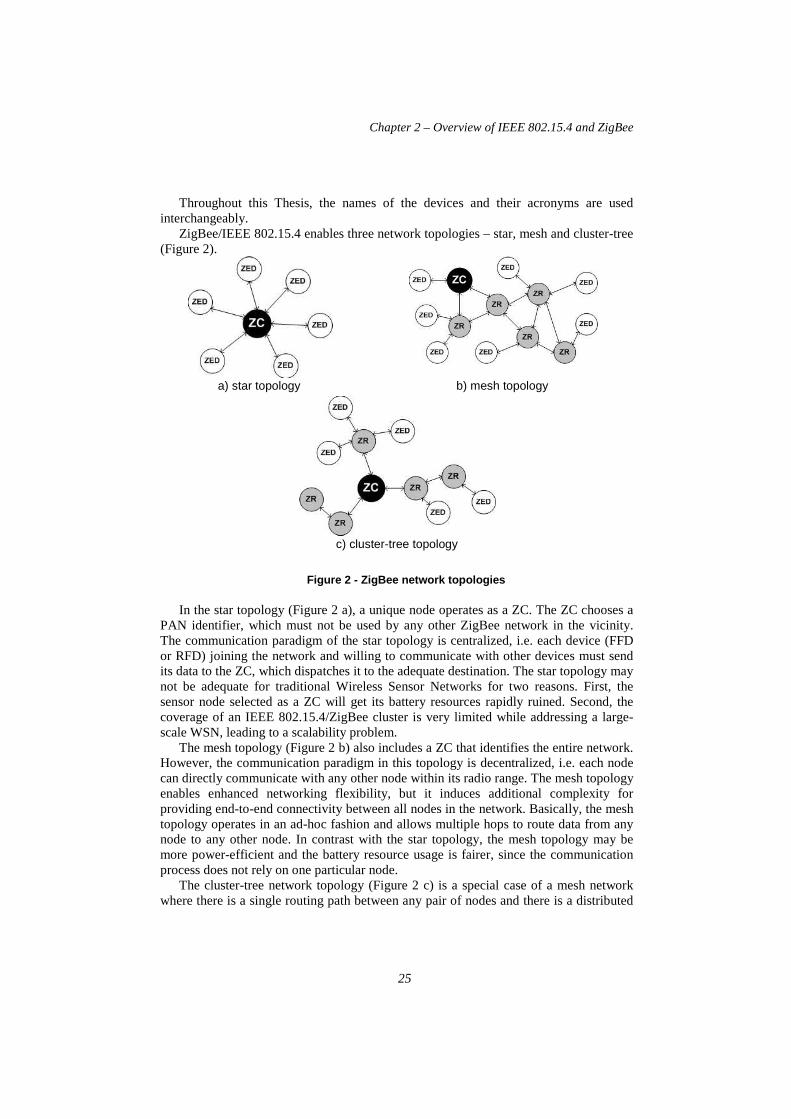
ZigBee/IEEE 802.15.4 enables three network topologies – star, mesh and cluster-tree (Figure 2).
a) star topology b) mesh topology
c) cluster-tree topology
Figure 2 - ZigBee network topologies
In the star topology (Figure 2 a), a unique node operates as a ZC. The ZC chooses a PAN identifier, which must not be used by any other ZigBee network in the vicinity. The communication paradigm of the star topology is centralized, i.e. each device (FFD or RFD) joining the network and willing to communicate with other devices must send its data to the ZC, which dispatches it to the adequate destination. The star topology may not be adequate for traditional Wireless Sensor Networks for two reasons. First, the sensor node selected as a ZC will get its battery resources rapidly ruined. Second, the coverage of an IEEE 802.15.4/ZigBee cluster is very limited while addressing a large-scale WSN, leading to a scalability problem.
The mesh topology (Figure 2 b) also includes a ZC that identifies the entire network. However, the communication paradigm in this topology is decentralized, i.e. each node can directly communicate with any other node within its radio range. The mesh topology enables enhanced networking flexibility, but it induces additional complexity for providing end-to-end connectivity between all nodes in the network. Basically, the mesh topology operates in an ad-hoc fashion and allows multiple hops to route data from any node to any other node. In contrast with the star topology, the mesh topology may be more power-efficient and the battery resource usage is fairer, since the communication process does not rely on one particular node.
The cluster-tree network topology (Figure 2 c) is a special case of a mesh network where there is a single routing path between any pair of nodes and there is a distributed

Chapter 2 – Overview of IEEE 802.15.4 and ZigBee
26
synchronization mechanism (IEEE 802.15.4 beacon-enabled mode). There is only one ZC which identifies the entire network and one ZR per cluster. Any of the FFD can act as a ZR providing synchronization services to other devices and ZRs.
Table 1 summarizes some of the differences between ZigBee mesh and cluster-tree topologies.
Table 1 – ZigBee Mesh vs. Cluster-Tree
The synchronization (beacon-enabled mode) feature of the cluster-tree model may be
seen both as an advantage and as a disadvantage, as reasoned next. On one hand, synchronization enables dynamic duty-cycle management in a per
cluster basis, allowing nodes (ZEDs and ZRs) to save their energy by entering the sleep mode. In contrast, in the mesh topology as defined in the IEEE 802.15.4 standard specification, only the ZEDs can have inactive periods. These energy saving periods enable the extension of the network lifetime, which is one of the most important requirements of WSNs. In addition, synchronization allows the dynamic reservation of guaranteed bandwidth in a per-cluster basis, through the allocation of Guaranteed Time Slots in the Superframe Contention Free Period (CFP). This enables the worst-case dimensioning of cluster-tree ZigBee networks, namely it is possible to compute worst-case message end-to-end delays and ZigBee Router buffer requirements.
On the other hand, managing the synchronization mechanism throughout the cluster-tree networks is a very challenging task. Even if we can cope with minor synchronization drifts between ZRs, this problem can grow for larger cluster-tree networks (higher depths). As previously mentioned, the de-synchronization of a cluster-tree network leads to collision problems due to overlapping Beacons and Superframes. For instance, the CAP of one cluster can overlap the CFP of another cluster, which is not admissible.
Regarding the routing protocols, the tree routing protocol in the cluster-tree is lighter that the mesh routing protocol (AODV) in terms of memory and processing requirements. The routing overhead, as compared with the AODV [22] in the mesh topology, is reduced. Note that the tree routing protocol considers just one path from any

Chapter 2 – Overview of IEEE 802.15.4 and ZigBee
27
source to any destination, thus it does not consider redundant paths, in contrast to AODV. Therefore, the tree routing protocol is prone to the single point of failure problem, while that can be avoided in mesh networks if alternative routing paths are available (more than one ZigBee Router within radio coverage).
Note that if there is a fault in a ZigBee Router, network inaccessibility times may be inadmissible for applications with critical timing and reliability requirements. Therefore, designing and engineering energy and time-efficient fault-tolerance mechanisms to avoid or at least minimize the single point of failure problem in ZigBee cluster-tree networks is of crucial importance.
Besides the Beacon/Superframe scheduling and the single-point-of-failure problems, there are other implementation-related obstacles that makes the use of the cluster-tree topology a challenging task, such as: (1) the dynamic network resynchronization, for instance in case of a new cluster joining or leaving the network; (2) the dynamic rearrangement of the all the duty cycles in the case of a router failure; (3) a new router association or even rearranging the superframe duration of some routers to adapt the bandwidth allocated to that branch of the tree; (4) the rearrangement of the addressing space allocated to each router; and (5) supporting mobility of nodes, routers or even hole clusters.
From our perspective, all these impairments have lead to the lack of commercial or academic solutions based on the ZigBee cluster-tree model. Nevertheless, we consider this model as a promising and adequate solution for WSN applications with timeliness and energy-efficiency requirements, which triggered us to implement it and explore its potential.
2.2 ZigBee Network Layer The ZigBee Network Layer is responsible for network management (e.g. association/disassociation, starting the network, addressing, device configuration and the maintenance of the NIB - NWK Information Base) and formation, message routing and security-related services.
The ZigBee Network Layer supports two service entities. The Network Layer Data Entity (NLDE) provides a data service, allowing the transmission of data frames and topology specific routing. Figure 3 depicts the Network Layer reference model.
Figure 3 - Network Layer reference model [7]

Chapter 2 – Overview of IEEE 802.15.4 and ZigBee
28
Joining and leaving a network must be supported by all ZigBee Devices. Both ZigBee Coordinators and Routers must support the following additional functionalities:
− Permit devices to join the network using the following: − Association indications from the MAC sub-layer; − Explicit join requests from the application.
− Permit devices to leave the network using the following: − Network Leave command frames; − Explicit leave requests from the application.
− Participate in assignment of logical network addresses. − Maintain a list of neighbouring devices.
The ZigBee Coordinator also defines some important additional network parameters. It determines the maximum number of children (Cm) any device is allowed to have. From this set of children, a maximum number (Rm) of devices can be router-capable devices. The remaining are ZEDs. Every device has an associated depth, representing the number of hops a transmitted frame must travel, using only a parent-child links, to reach the ZigBee Coordinator. The ZC has a depth of 0, while its children have a depth of 1. The ZC also determines the maximum depth (Lm) of the network. The maximum number of children, routers and network depth are used for calculating the addresses of the devices in the network, in a distributed address scheme.
2.2.1 Short Address Assignment A parent device uses the Cm, Rm, and Lm values to compute a Cskip function defining the size of the address sub-block that is distributed by each parent depending on its depth (d) in the network. For a given network depth d, Cskip(d) is calculated as follows:
−⋅−−+
=−−⋅+= −−
Otherwise ,Rm1
RmCmRmCm1 1Rm if ),1dLm(Cm1
)d(Cskip 1dLm (2.1)
A parent device that has a Cskip(d) value of zero is not capable of accepting children
and must be treated as an end device. A parent device that has a Cskip(d) value greater that zero must accept devices and assigns addresses if possible. A parent device assigns an address that is one greater than its own to the first router that associated. The next associated router receives an address that is separated according to the return value of the Cskip(parent depth) function. The maximum number of associated routers is defined in the network parameter nwkMaxRouters (Rm).
Considering a parent node with a depth d and an address of Aparent, the number of child devices n is between 1 and Cm-Rm.
( )mm RCn1 −≤≤ (2.2)
The Achild address of the nth child router is calculated according to Eq. 2.3(n is the
number of child routers):

Chapter 2 – Overview of IEEE 802.15.4 and ZigBee
29
0 1 32 63 94 125
126
33 40 47 54 55 56 57 58 59 6032
ZigBee Coordinator (0x0000)
ZigBee Router (0x0020)
( ) ( )( ) ( ) 1n,dCskip1nAA
1n,1dCskip1nAA
parentchild
parentchild
>×−+=
=+×−+= (2.3)
The Achild address of the nth child end device is calculated according to Eq. 2.4 (n is
the number of child end devices):
( ) ndCskipRmAA parentchild +×+= (2.4)
Figure 4 depicts an example of an address assignment scheme. The parameters used
in the address assignment are the following: maximum depth (Lm) = 3, maximum children (Cm) = 6 and maximum routers (Rm) = 4.
Figure 4 - Address assignment scheme example
Figure 5 shows the ZigBee Coordinator (0x0000) available addressing scheme. Considering the above network parameters, the ZigBee Coordinator is allowed to associate up to A4 routers and 2 end devices in its available address pool. On the other hand, the ZR (0x0020) is allowed to associate up to 4 ZRs and 6 ZEDs.
Figure 5 - ZigBee Coordinator addressing scheme (de cimal values)
Depth = 0 Cskip(0) = 31
Depth = 1 Cskip(1) = 7
Depth = 2 Cskip(2) = 1

Chapter 2 – Overview of IEEE 802.15.4 and ZigBee
30
2.2.2 ZigBee Routing ZigBee Coordinators and Routers must provide the following functionalities:
− Relay data frames on behalf of higher layers; − Relay data frames on behalf of other ZR; − Participate in route discovery in order to establish routes for subsequent data
frames; − Participate in route discovery on behalf of end devices; − Participate in end-to-end route repair; − Participate in local route repair; − Employ the ZigBee path cost metric as specified in route discovery and route
repair. Additionally, ZigBee Coordinators and Routers may provide the following
functionalities: − Maintain routing tables in order to remember best available routes; − Initiate route discovery on behalf of higher layers; − Initiate route discovery on behalf of other ZR; − Initiate end-to-end route repair; − Initiate local route repair on behalf of other ZR.
2.2.3 Routing Schemes ZigBee Coordinators and Routers support three types of routing:
− Neighbour Routing – based on a neighbour tables that contains the information of all the devices within radio coverage. If the target device is physically in range the message can be sent directly. Note that ZEDs cannot do this.
− Table Routing - Ad-hoc On Demand Distance Vector (AODV) [22], based on routing and route discovery tables with the path cost metrics;
− Tree-Routing - based on the address assignment schemes; messages are hierarchically routed upstream/downstream the tree.
Neighbour Routing This type of routing uses the neighbour tables. If the target device is physically in range it is possible to send messages directly to the destination. Physically in range means that the source ZC or ZR has a neighbour table entry for the destination. This routing mechanism is mostly used as addition to other routing mechanisms and for the ZigBee Routers to route messages to its children devices, when they are the destination.
Table Routing - Ad-hoc On-Demand Distance Vector (AODV) ZigBee Table Routing is based on the AODV routing algorithms. Each ZigBee Coordinator and Router that supports this Table Routing must maintain two tables: (1) the routing table, a long-lived and persistent table with the information of routes, and (2) a route discovery table with the information of the route discovery procedures where each entry only lasts the duration of the discovery.

Chapter 2 – Overview of IEEE 802.15.4 and ZigBee
31
The Ad-hoc On Demand Distance Vector (AODV) [22] routing protocol was designed for ad hoc mobile networks. AODV is capable of both unicast and multicast routing. AODV allows mobile nodes to obtain routes quickly for new destinations, and does not require nodes to maintain routes to destinations that are not in active communication. AODV allows mobile nodes to respond to link breakages and changes in network topology in a timely manner. The operation of AODV is loop-free, and by avoiding the Bellman-Ford "counting to infinity" problem offers quick convergence when the ad-hoc network topology changes (typically, when a node moves in the network). When the link breaks, AODV causes the affected set of nodes to be notified so that they are able to invalidate the routes using the lost link. It is an on demand algorithm, meaning that it builds routes between nodes only if requested by source nodes. It maintains these routes as long as they are needed by the sources. Additionally, AODV can form trees, connecting multicast groups, composed of the group members and the nodes needed to connect. AODV uses sequence numbers to ensure the freshness of routes. It is loop-free, self-starting, and scales to larger numbers of nodes.
In ZigBee Networks, the routing management is done by the means of NWK
command frames. The available commands are the following: − Route request – Command send to search for a route to a specified device, can
also be used to repair a route − Route reply – Command send in response of a route request, also used to request
state information − Route Error – notification of a source device of the data frame about the failure in
forwarding the frame: − Leave – notification of a device leaving the network − Route Record – notification of a list of nodes used in relaying a data frame − Rejoin request – notification of a device rejoining the network − Rejoin response – rejoin response of a rejoin request
The route choice for a communication flow is based on the total link cost represented
by C, meaning that the path with the lowest cost is chosen. The total link cost is the sum of individual point-to-point link cost.
The calculation of C is as follows: for a defined path P where L defines the length of a set of devices [D 1,D2, … DL] and a link [D i, Di+1] the path cost C is defined as:
{ } [ ]{ }∑−
=+=
1
111,
L
iiDDCPC (2.5)
Each C{[D 1,Di+1]} is the individual point-to-point link cost, calculated by the
following formulation:
{ }
=4
1,7min
,7
lproundlC
(2.6)
where pl is defined as the probability of packet delivery through link l.

Chapter 2 – Overview of IEEE 802.15.4 and ZigBee
32
The link probability estimation factors are implementation specific, but generally it they are based on the counting of the received beacons and data frames in order to detect packet loss and in the estimation of the Link Quality Indicator (LQI).
Tree-Routing This routing mechanism is based on the short addressing scheme and was initially proposed by MOTOROLA [23]. Each device, upon the reception of a data frame, reads the routing information fields and checks the destination address. If the destination is a child of the device (neighbour table check), the device relays the packet to the appropriate address. If the destination address is not a child, the device must check if the address is a descendent using the condition in 2.7, where A is device network address, D the destination address and d the device depth in the network.
( )1dCskipADA −+<< (2.7)
The next hop (N) address when routing down is given by:
)()(
)1(1 dCskip
dCskip
ADAN ×
+−++= (2.8)
If the destination address is not a descendant, the device relays the packet to its
parent. Consider the network scenario illustrated in Figure 4 and the following network
parameters: Lm = 3; Cm = 6; Rm = 4. The Cskip values are presented in Table 2.
Table 2 - Cskip example values
Depth Cskip(Depth) 0 31 1 7 2 1
If ZR 0x0002 transmits a message to ZR 0x0028, the tree-routing protocol behaves as follows:
1. ZR 0x0002 builds the data frame and sends it to its parent (0x0001). The most relevant fields of this data frame are outlined next:
− MAC destination address – 0x0001;
− MAC source address – 0x0002;
− Network Layer Routing Destination Address – 0x0028;
− Network Layer Routing Source Address – 0x0002;
2. ZR 0x0001 receives the data frame, realizes that the message in not for him and has to be relayed. The device checks its neighbour table for the routing destination address, trying to find if the destination is one of its child devices. Then, the device

Chapter 2 – Overview of IEEE 802.15.4 and ZigBee
33
checks if the routing destination address is a descendant by verifying condition in 2.7 that results in:
0x0001 < 0x0028 < 0x0001 + 7
Note that ZR 0x0001 is a depth 1 device in the network. After verifying that the
destination is not a descendant, ZR 0x0001 routes the data frame to its parent, ZC 0x0000. The most relevant fields of this data frame are outlined next:
− MAC destination address – 0x0000;
− MAC source address – 0x0001;
− Network Layer Routing Destination Address – 0x0028;
− Network Layer Routing Source Address – 0x0002;
3. ZC 0x0000 receives the data frame and verifies if the routing destination address exists in its neighbour table. After realizing that the destination device is not its neighbour, since the ZC is the root of the tree and cannot route up, the next hop address is calculated as follows:
3131
)100000(00280100000 ×
+−++= xxxN
The next hop address results in N = 32 (decimal) = 0x0020. The most relevant fields
of this data frame are outlined next:
− MAC destination address – 0x0020;
− MAC source address – 0x0000;
− Network Layer Routing Destination Address – 0x0028;
− Network Layer Routing Source Address – 0x0002;
4. ZR 0x0020 receives the data frame and checks its neighbour table for the routing destination address. After verifying that the address is its neighbour, the message is routed to it. The next hop is assigned with the short address present in the respective neighbour table entry. The most relevant fields of this data frame are outlined next:
− MAC destination address – 0x0028;
− MAC source address – 0x0020;
− Network Layer Routing Destination Address – 0x0028;
− Network Layer Routing Source Address – 0x0002;
2.3 IEEE 802.15.4 Protocol Standard The IEEE 802.15.4 Full Function Devices (FFD) have three different operation modes:
− The Personal Area Network (PAN) Coordinator: the principal controller of the PAN. This device identifies its own network as well as its configurations, to

Chapter 2 – Overview of IEEE 802.15.4 and ZigBee
34
which other devices may be associated. In ZigBee, this device is referred to as the ZigBee Coordinator (ZC).
− The Coordinator: provides synchronization services through the transmission of beacons. This device should be associated to a PAN Coordinator and does not create its own network. In ZigBee, this device is referred to as the ZigBee Router (ZR).
− The End Device: a device which does not implement the previous functionalities and should associate with a ZC or ZR before interacting with the network. In ZigBee, this device is referred to as the ZigBee End Device (ZED).
The Reduced Function Device (RFD) is an end device operating with the minimal
implementation of the IEEE 802.15.4. An RFD is intended for applications that are extremely simple, such as a light switch or a passive infrared sensor; they do not have the need to send large amounts of data and may only associate with a single FFD at a time.
Throughout this Thesis the IEEE 802.14.5 operational modes and the ZigBee device names are used interchangeably (e.g. PAN Coordinator = ZigBee Coordinator, Coordinator = ZigBee Router and End Device = ZigBee End Device). The designation of Coordinator represents both ZC and ZRs.
2.3.1 Physical Layer The IEEE 802.15.4 physical layer is responsible for data transmission and reception using a certain radio channel and according to a specific modulation and spreading technique.
The IEEE 802.15.4 offers three operational frequency bands: 2.4 GHz, 915 MHz and 868 MHz (Figure 6). There is a single channel between 868 and 868.6 MHz (20 kbit/s), 10 channels between 902 and 928 MHz (40 kbit/s), and 16 channels between 2.4 and 2.4835 GHz (250 kbit/s). The protocol also allows dynamic channel selection, a channel scan function in search of a beacon, receiver energy detection, link quality indication and channel switching.
Figure 6 - Operating frequencies and bands [24]

Chapter 2 – Overview of IEEE 802.15.4 and ZigBee
35
All of these frequency bands are based on the Direct Sequence Spread Spectrum (DSSS) spreading technique.
The physical layer of IEEE 802.15.4 is in charge of the following tasks:
− Activation and deactivation of the radio transceiver: The radio transceiver may operate in one of three states: transmitting, receiving or sleeping. Upon request of the MAC sub-layer, the radio is turned ON or OFF. The turnaround time from transmitting to receiving and vice versa should be no more than 12 symbol periods, according to the standard (each symbol corresponds to 4 bits).
− Energy Detection (ED): Estimation of the received signal power within the bandwidth of an IEEE 802.15.4 channel. This task does not make any signal identification or decoding on the channel. The energy detection time should be equal to 8 symbol periods. This measurement is typically used by the Network Layer as a part of channel selection algorithm or for the purpose of Clear Channel Assessment (CCA), to determine if the channel is busy or idle.
− Link Quality Indication (LQI): Measurement of the Strength/Quality of a received packet. It measures the quality of a received signal. This measurement may be implemented using receiver ED, a signal to noise estimation or a combination of both techniques.
− Clear Channel Assessment (CCA): Evaluation of the medium activity state: busy or idle. The CCA is performed in three operational modes: (1) Energy Detection mode: the CCA reports a busy medium if the detected energy is above the ED threshold. (2) Carrier Sense mode: the CCA reports a busy medium only is it detects a signal with the modulation and the spreading characteristics of IEEE 802.15.4 and which may be higher or lower than the ED threshold. (3) Carrier Sense with Energy Detection mode: this is a combination of the aforementioned techniques. The CCA reports that the medium is busy only if it detects a signal with the modulation and the spreading characteristics of IEEE 802.15.4 and with energy above the ED threshold.
− Channel Frequency Selection: The IEEE 802.15.4 defines 27 different wireless channels. Each network can support only part of the channel set. Hence, the physical layer should be able to tune its transceiver into a specific channel when requested by a higher layer.
2.3.2 Medium Access Control (MAC) Sub-layer The MAC protocol supports two operational modes (Figure 7): − The non beacon-enabled mode. When the ZC selects the non-beacon enabled
mode, there are neither beacons nor superframes. Medium access is ruled by an unslotted CSMA/CA mechanism (refer to Section 2.2.6).
− The beacon-enabled mode. In this mode, beacons are periodically sent by the ZC or ZR to synchronize nodes that are associated with it, and to identify the PAN. A beacon frame delimits the beginning of a superframe (refer to Section 2.2.3) defining a time interval during which frames are exchanged between different nodes in the PAN. Medium access is basically ruled by Slotted CSMA/CA. However, the beacon-enabled mode also enables the allocation of contention free time slots, called Guaranteed Time Slots (GTSs) for nodes requiring guaranteed bandwidth.

Chapter 2 – Overview of IEEE 802.15.4 and ZigBee
36
Figure 7 - IEEE 802.15.4 Operational Modes
Superframe Structure The superframe is defined between two beacon frames and has an active period and an inactive period. Figure 8 depicts the IEEE 802.15.4 superframe structure.
Figure 8 - IEEE 802.15.4 Superframe Structure [24]
The active portion of the superframe structure is composed of three parts, the
Beacon, the Contention Access Period (CAP) and the Contention Free Period (CFP): − Beacon: the beacon frame is transmitted at the start of slot 0. It contains the
information on the addressing fields, the superframe specification, the GTS fields, the pending address fields and other PAN related.
− Contention Access Period (CAP): the CAP starts immediately after the beacon frame and ends before the beginning of the CFP, if it exists. Otherwise, the CAP ends at the end of the active part of the superframe. The minimum length of the CAP is fixed at aMinCAPLength = 440 symbols. This minimum length ensures that MAC commands can still be transmitted when GTSs are being used. A temporary violation of this minimum may be allowed if additional space is needed to temporarily accommodate an increase in the beacon frame length, needed to perform GTS management. All transmissions during the CAP are made using the Slotted CSMA/CA mechanism. However, the acknowledgement frames and any data that immediately follows the acknowledgement of a data request command are transmitted without

Chapter 2 – Overview of IEEE 802.15.4 and ZigBee
37
contention. If a transmission cannot be completed before the end of the CAP, it must be deferred until the next superframe.
− Contention Free Period (CFP): The CFP starts immediately after the end of the CAP and must complete before the start of the next beacon frame (if BO equals SO) or the end of the superframe. Transmissions are contention-free since they use reserved time slots (GTS) that must be previously allocated by the ZC or ZR of each cluster. All the GTSs that may be allocated by the Coordinator are located in the CFP and must occupy contiguous slots. The CFP may therefore grow or shrink depending on the total length of all GTSs.
In beacon-enabled mode, each Coordinator defines a superframe structure Figure 8 which is constructed based on:
− The Beacon Interval (BI), which defines the time between two consecutive beacon frames;
− The Superframe Duration (SD), which defines the active portion in the BI, and is divided into 16 equally-sized time slots, during which frame transmissions are allowed.
Optionally, an inactive period is defined if BI > SD. During the inactive period (if it exists), all nodes may enter in a sleep mode (to save energy). BI and SD are determined by two parameters, the Beacon Order (BO) and the Superframe Order (SO), respectively, as follows:
14BOSO0for2ionframeDurataBaseSuperSD
2ionframeDurataBaseSuperBISO
BO
≤≤≤
×=
×= (2.9)
aBaseSuperframeDuration = 15.36 ms (assuming 250 kbps in the 2.4 GHz frequency band) denotes the minimum duration of the superframe, corresponding to SO=0.
As depicted in Figure 8, low duty cycles can be configured by setting small values of the SO as compared to BO, resulting in greater sleep (inactive) periods. In ZigBee Cluster-Tree networks, each cluster can have different and dynamically adaptable duty-cycles. This feature is particularly interesting for WSN applications, where energy consumption and network lifetime are main concerns. Additionally, the Guaranteed Time Slot (GTS) mechanism is quite attractive for time-sensitive WSNs, since it is possible to guarantee end-to-end message delay bounds both in Star and Cluster-Tree topologies.
Association and Channel Scan Mechanisms The association procedure takes place when a device wants to associate with a Coordinator. This mechanism can be divided into three separate phases: (1) channel scan procedure; (2) selection of a possible parent; (3) association with the parent.
IEEE 802.15.4 enables four types of channel scan procedures: (1) the energy detection scan, where the device obtains a measure of the peak energy in each channel; (2) the active scan, where the device locates all Coordinators transmitting beacon frames; this scan is performed on each channel by first transmitting a beacon request command; (3) the passive scan, where similarly to the active scan, the device locates all Coordinator transmitting beacon frames with the difference that the scan is performed only in a receive mode, without transmitting beacon requests; and (4) the orphan scan, used to locate the Coordinator with which the scanning device had previously associated.

Chapter 2 – Overview of IEEE 802.15.4 and ZigBee
38
After the channel scan procedure is completed, the NWK layer receives a list of all detected PAN descriptors (containing information about the potential parents). Based on the information collected during the scan, the device can choose the most suitable parent (that permits associations). The IEEE 802.15.4 protocol standard leaves the way to take the association decision to the system designer. Nevertheless one of the most relevant parameters to be considered is the Link Quality Indicator (LQI).
For a device to associate to a Coordinator, it must send an association command frame. Then, if the Coordinator accepts the device, it adds it to its neighbour table as its child. An association response command frame is, in the case of a successful association, sent to the device (via an indirect transmission, refer to Section 2.2.8), embedding its short address. Otherwise, in the case of an unsuccessful association, the association response embeds the problem status information. The Coordinator replies to the association command frame with an acknowledgment embedding the pending data control flag active, meaning that it has data ready to be transmitted to the device. The association procedure is completed when the device sends a data request command frame to the Coordinator requesting the pending data (the association response command). After a successful association, the device stores all the information about the new PAN by updating its MAC PAN Information Base (MAC PIB) and can start transmissions. Figure 9 exemplifies the sequence of messages for a successful association request, followed by a data transmission.
The disassociation from a Coordinator is done via a disassociation request command. The disassociation can be initiated either by the device or by the Coordinator. After the disassociation procedure, the device loses its short address and is not able to communicate.
Figure 9 - Association mechanism example

Chapter 2 – Overview of IEEE 802.15.4 and ZigBee
39
The Coordinator updates the list of associated devices, but it can still keep the device information for a future re-association. Figure 10 shows a transmission sequence of a disassociation request initiated by a device.
Figure 10 - Dissassociation mechanism example
Guaranteed Time Slot (GTS) mechanism The GTS mechanism allows devices to access the medium without contention, in the CFP. GTSs are allocated by the Coordinator and are used only for communications between the Coordinator and a device. Each GTS may contain one or more time slots. The Coordinator may allocate up to seven GTSs in the same superframe, provided that there is sufficient capacity in the superframe. Each GTS has only one direction: from the device to the Coordinator (transmit) or from the Coordinator to the device (receive). Figure 11 illustrates message sequence diagram for a GTS allocation.
Figure 11 - GTS allocation message sequence diagram [24]
The GTS can be deallocated at any time at the discretion of the Coordinator or the device that originally requested the GTS allocation. A device to which a GTS has been allocated can also transmit during the CAP. The Coordinator is the responsible for performing the GTS management; for each GTS, it stores the starting slot, length, direction, and associated device address. All these parameters are embedded in the GTS request command. Only one transmit and/or one receive GTS are allowed for each device. Upon the reception of the deallocation request the Coordinator updates the GTS descriptor list by removing the previous allocated slot and rearranging the remaining allocation starting slots. The arrangement of the CFP consists in shifting right the
Chapter 2 – Overview of IEEE 802.15.4 and ZigBee
40
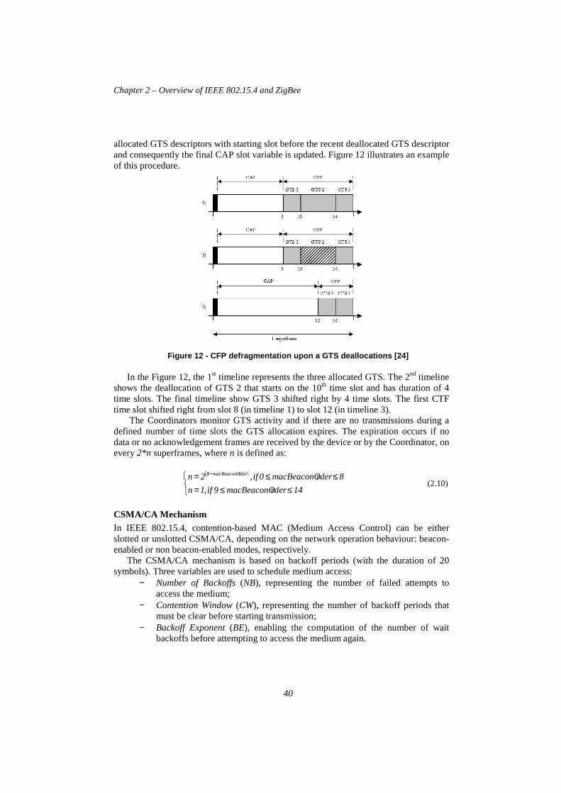
allocated GTS descriptors with starting slot before the recent deallocated GTS descriptor and consequently the final CAP slot variable is updated. Figure 12 illustrates an example of this procedure.
Figure 12 - CFP defragmentation upon a GTS dealloca tions [24]
In the Figure 12, the 1st timeline represents the three allocated GTS. The 2nd timeline shows the deallocation of GTS 2 that starts on the 10th time slot and has duration of 4 time slots. The final timeline show GTS 3 shifted right by 4 time slots. The first CTF time slot shifted right from slot 8 (in timeline 1) to slot 12 (in timeline 3).
The Coordinators monitor GTS activity and if there are no transmissions during a defined number of time slots the GTS allocation expires. The expiration occurs if no data or no acknowledgement frames are received by the device or by the Coordinator, on every 2*n superframes, where n is defined as:
( )
≤≤=≤≤= −
14rdermacBeaconO9if,1n
8rdermacBeaconO0if,2n rdermacBeaconO8 (2.10)
CSMA/CA Mechanism In IEEE 802.15.4, contention-based MAC (Medium Access Control) can be either slotted or unslotted CSMA/CA, depending on the network operation behaviour: beacon-enabled or non beacon-enabled modes, respectively.
The CSMA/CA mechanism is based on backoff periods (with the duration of 20 symbols). Three variables are used to schedule medium access:
− Number of Backoffs (NB), representing the number of failed attempts to access the medium;
− Contention Window (CW), representing the number of backoff periods that must be clear before starting transmission;
− Backoff Exponent (BE), enabling the computation of the number of wait backoffs before attempting to access the medium again.

Chapter 2 – Overview of IEEE 802.15.4 and ZigBee
41
Figure 13 depicts a flowchart describing the slotted version of the CSMA/CA mechanism. It can be summarized in five steps:
1. initialization of the algorithm variables: NB equal to 0; CW equals to 2 and BE is set to the minimum value between 2 and a MAC sub-layer constant (macMinBE);
2. after locating a backoff boundary, the algorithm waits for a random defined number of backoff periods before attempting to access the medium;
3. Clear Channel Assessment (CCA) to verify if the medium is idle or not. 4. The CCA returned a busy channel, thus NB is incremented by 1 and the
algorithm must start again in Step 2; 5. The CCA returned an idle channel, CW is decremented by 1 and when it
reaches 0 the message is transmitted, otherwise the algorithm jumps to Step 3. In the slotted CSMA/CA, when the battery life extension is set to 0, the CSMA/CA
must ensure that, after the random backoff (step 2), the remaining operations can be undertaken and the frame can be transmitted before the end of the CAP. If the number of backoff periods is greater than the remaining in the CAP, the MAC sub-layer pause the backoff countdown at the end of the CAP and defers it to the start of the next superframe. If the number of backoff periods is less or equal than the remaining number of backoff periods in the CAP, the MAC sub-layer applies the backoff delay and re-evaluate whether it can proceed with the frame transmission. If the MAC sub-layer do not have enough time, it defers until the start of the next superframe, continuing with the two CCA evaluations (step 3). If the battery life extension set to 1, the backoff countdown must only occur during the first six full backoff periods, after the reception of the beacon, as the frame transmission must start in one of these backoff periods.
Figure 13 - The Slotted CSMA/CA Mechanism [24]

Chapter 2 – Overview of IEEE 802.15.4 and ZigBee
42
The non slotted mode of the CSMA/CA (Figure 14) is very similar to the slotted version except the algorithm does not need to rerun (CW number of times) when the channel is idle.
Figure 14 - The Un-slotted CSMA/CA mechanism [24]
Inter-Frame Spacing (IFS) The inter-frame spacing (IFS) is an idle communication period that is needed for supporting the MAC sub-layer needs to process data received by the physical layer. To allow this, all transmitted frames are followed by an IFS period. If the transmission requires an acknowledgment, the IFS will follow the acknowledgement frame. The length of the IFS period depends on the size of the transmitted frame: a long inter-frame spacing (LIFS) or short inter-frame spacing (SIFS). The selection of the IFS is based on the IEEE 802.15.4 aMaxSIFSFrameSize parameter, defining the maximum allowed frame size to use the SIFS. The CSMA/CA algorithm takes the IFS value into account for transmissions in the CAP. These concepts are illustrated in Figure 15.
Figure 15 - Inter-frame spacing [24]

Chapter 2 – Overview of IEEE 802.15.4 and ZigBee
43
Transmission scenarios and reception conditions The IEEE 802.15.4 protocol standard enables three different types of transmissions:
1. Direct transmissions – the frames are transmitted to the medium without any channel assessment i.e. the beacon frames, the acknowledgment frames and the frames in the GTS time slots;
2. Indirect transmissions – the frames are stored in the Coordinator to which the destination device is associated. Then, the information about the stored frames (or pending transmissions) is included in the pending addresses descriptors fields of the beacon frame. If a device has pending data in the Coordinator it can request it by sending a data request command frame. An example of this mechanism is depicted in Figure 16 where the Coordinator beacon contains the short address 0x0004 in the pending address list. In the Coordinator neighbour table, the short address 0x0004 is associated to the extended address 0x0000000400000004. Then, the device 0x0004 requests the data with a data request message embedding its extended address. The Coordinator searches in its neighbour tables for the short address corresponding to the extended address received in the command frame and transmit the corresponding pending data. In the next Coordinator beacon the pending address list is updated.
3. Normal transmissions – the frames are transmitted to the medium with contention, by applying the CSMA/CA algorithm i.e. data frames and command frames transmitted during the CAP. Depending of the operation mode (beacon-enabled or non beacon-enabled) the CSMA/CA algorithm has two versions, the slotted or the unslotted respectively.
Figure 16 - Indirect transmission example
The IEEE 802.15.4 protocol standard identifies three different transmissions scenarios during the CAP:
− Successful data transmission– the sender successfully transmits the frame to the intended recipient. The recipient receives the frame and sends an acknowledgment if required. If it is an acknowledged request, the sender starts a timer that expires after macAckWaitDuration symbols. Upon the reception of the acknowledge frame (before the timer expires), the sender disables and reset the timer. The data transfer is completed successfully.

Chapter 2 – Overview of IEEE 802.15.4 and ZigBee
44
− Loss of frame – the sender successfully transmits the frame to the medium but it never reaches the destination, so that an acknowledgement frame is not transmitted. The sender timer expires (after macAckWaitDuration) and the sender retransmits the frame again. This procedure is repeated up to a maximum of aMaxFrameRetries times after which the transmission aborts.
− Loss of acknowledgment - the sender successfully transmits the frame to the intended recipient that upon reception replies with an acknowledgement frame. The sender never receives the acknowledgment and retries the transmission.
The MAC sub-layer will only accept frames from the Phy layer if it satisfies the
following requirements: − The frame type subfield of the frame control field does not contain an illegal
frame type; − If the frame type indicates that the frame is a beacon frame, the source PAN
identifier must match macPANId, unless macPANId is equal to 0xffff, in which case the beacon frame must be accepted regardless of the source PAN identifier;
− If a destination PAN identifier is included in the frame, it must match macPANId or the broadcast PAN identifier (0xffff);
− If a short destination address is included in the frame, it must match either macShortAddress or the broadcast address (0xffff). Otherwise, if an extended destination address is included in the frame, it must match aExtendedAddress;
− If only source addressing fields are included in a data or MAC command frame, the frame is accepted only if the device is a Coordinator and the source PAN identifier matches macPANId.

Chapter 3 Technological Platforms and Tools
This chapter describes the technologies used to carry out all of the implementation and experimental work presented in this Thesis, like the WSN platforms and network analysers used for debugging and analysis. It also presents some of the Open-ZB tools like the TinyOS IEEE 802.15.4/ZigBee protocol stack implementation and the OPNET simulation model.
3.1 Mote Platforms – The MICAz and TelosB The Open-ZB [19] IEEE 802.15.4/ZigBee implementation is supported by two hardware platforms, the MICAz [25] and the TelosB [26] motes. The MICAz mote (Figure 17 left) has the following features:
− ATMEL ATmega128L 8-bit microcontroller [27]; − CC2420 RF transceiver [28]; − 128 KB of Program memory (in-system reprogrammable flash); − 4 KB of EEPROM; − Supports several sensor boards; − UART communication port.

Chapter 3 – Technological Platforms and Tools
Figure
The TelosB mote (Figure − TI MSP430 16-− CC2420 RF transceiver− 48 KB of Program memory (in− 10 KB of EEPROM;− Includes a temperature and light sensor;− UART communication port (USB converter).
Figure
The TelosB architecture is slightly different from the one of the MICAz, especially due to the 16-bits MSP430 microcontroller Atmega128 microcontroller driver modules already provided in TinyOS and the adaptation of the first implementation version, which only supported the MICAz platform, to s
Technological Platforms and Tools
46
Figure 17 - Micaz mote and the block diagram [25]
Figure 18 left) has the following characteristics: -bit microcontroller [29] ;
CC2420 RF transceiver [28]; 48 KB of Program memory (in-system reprogrammable flash); 10 KB of EEPROM; Includes a temperature and light sensor; UART communication port (USB converter).
Figure 18 - TelosB mote and the block diagram [26]
The TelosB architecture is slightly different from the one of the MICAz, especially bits MSP430 microcontroller [29] as compared to the MICAz 8
Atmega128 microcontroller [27]. This triggers the need for selecting the corresponding driver modules already provided in TinyOS and the adaptation of the first implementation version, which only supported the MICAz platform, to support the 16
The TelosB architecture is slightly different from the one of the MICAz, especially as compared to the MICAz 8-bits
. This triggers the need for selecting the corresponding driver modules already provided in TinyOS and the adaptation of the first
upport the 16-

Chapter 3 – Technological Platforms and Tools
47
bits memory block of the MSP430. Both platforms use the same 2.4 GHz Chipcon CC2420 radio transceiver [28].
3.2 The FLEX Board The FLEX [30] was built as an embedded board to exploit the potential of the Microchip micro-controllers: the dsPIC family, aiming at the development and test of real-time applications.
Its main features are: − DsPIC33FJ256MC710 Microcontroller at 40 MHz [31]; − Flexipanel EASYBEE IEEE 802.15.4 Transceiver module [32]; − 256 KB of Program memory (in-system reprogrammable flash); − modular architecture (done by using daughter boards piggybacking); − ICD2 in-circuit programmer connector; − the full support of the ERIKA real-time kernel from Evidence Srl;
The compact design allows the employment of FLEX not only for development
purposes, but also as a suitable solution for the direct deployment of Wireless, Acquisition, and Digital control systems. The basic configuration of a FLEX device is made by the Base Board. The FLEX Base Board mounts a Microchip dsPIC micro-controller, and exports almost all the pins of the micro-controller. The user can easily connect the desired components to the dsPIC ports in order to build the specific application.
As depicted in Figure 19, several daughter boards can be connected in piggyback to the Flex Base Board. The daughter boards have different features and they can be easily combined to obtain complex devices.
Figure 19 - The FLEX board [30]
3.3 Programming Interfaces The TelosB motes do not need any programmer interface because they already have an USB port that can be used to upload programs as well as interfacing the mote with other equipments. However, the MICAz mote needs to be programmed using an interface board such as the MIB510 (Figure 20 A) [33], the MIB520 (Figure 20 B) [34], and the MIB600 (Figure 20 C) [35]. The interface boards MIB510 and MIB520 are very similar

Chapter 3 – Technological Platforms and Tools
48
except the fact the MIB510 has a serial RS-232 interface and the MIB520 has an USB interface. The MIB600 has an RJ-45 Ethernet interface with an implementation of the full TCP/IP protocol. These three interface boards allow the use of a JTAG adapter for debugging and can be used as base stations interfacing the wireless sensor network with a PC.
A) MIB510 [33] B) MIB520 [34] C) MIB600 [35]
Figure 20 - Interface Boards - MIB510, MIB520 and M IB600
The FLEX boards are programmed through a debugger/programmer device called MPLAB ICD2 [36] from Microchip. The MPLAB ICD 2 is a low cost, real-time debugger and programmer for selected PIC MCUs and dsPIC® DSCs. Using Microchip Technology's proprietary In-Circuit Debug functions, programs can be downloaded, executed in real time and examined in detail with the debug functions of MPLAB IDE. Set watch variables and breakpoints from symbolic labels in C or assembly source code, and single step through C source lines or into assembly code. MPLAB ICD 2 can also be used as a development programmer for supported MCUs since it is able to program or reprogram the Flash-based microcontroller while installed on the board.
Some of the features are: − USB (Full Speed 2 M bits/s) & RS-232 interface to host PC − Real time background debugging − MPLAB IDE GUI (free copy included) − Built in over-voltage/short circuit monitor − Firmware upgradeable from PC − Supports low voltage to 2.0 volts. (2.0 to 6.0 range) − Diagnostic LEDs (Power, Busy, Error) − Reading/Writing memory space and EEDATA areas of target microcontroller − Programs configuration bits − Erase of program memory space with verification − Peripheral freeze-on-halt stops timers at breakpoints
3.4 IEEE 802.15.4/ZigBee Protocol Analysers The implementation of the IEEE 802.15.4/ZigBee has been supported by two network protocol analysers (packet sniffers): the Chipcon CC2420 Packet Sniffer for IEEE 802.15.4 v1.0 [37] and the Daintree IEEE 802.15.4/ZigBee Network Analyser [38]. These analysers interpret the IEEE 802.15.4 and ZigBee frames, allowing to debug and to validate the implementation of the IEEE 802.15.4/ZigBee protocols.

Chapter 3 – Technological Platforms and Tools
49
a) Snapshot of the sniffer application [37]
b) CC2420 EB with a CC2420EM [38]
Figure 21 - Overview of the Chipcon IEEE802.15.4/Zi gBee Packet Sniffer
The packet sniffer provided by Chipcon (Figure 21), the CC2420 Packet Sniffer for IEEE 802.15.4 v1.0 provides a raw list of the packets transmitted. This application works in conjunction with a CC2400EB board (Figure 21.b) and a CC2420EM module (equipped with a CC2420 radio transceiver). Figure 21.a depicts a snapshot of the sniffer application which provides the following features:
− Raw list of the received packets with timestamp information; − Interpretation of the packets information, highlighting the different packet
fields; − Packet fields filtering; − Device list.
Chipcon also provides a tool used to test the transceivers, the SmartRF Studio [39].
This application interacts with the CC2420EB/CC2420EM evaluation board and allows viewing and interacting with the CC2420 transceiver memory registries. With this tool is possible to test different configurations on the transceiver and test its behaviour with simple send/receive functions. This tool was very useful during the protocol stack implementation enabling a better understanding of the physical layer implementation and the functionalities of the transceiver. Figure 22 depicts an overview example of the Smart RF application interfaces, which provides the following features:
Read/Write from/to the CC2420 transceiver memory registries (Figure 22.a); − Execute functions of the transceiver (e.g. TR ON, TX OFF, etc.) − Test transmissions, IEEE 802.15.4 compatible packets or an unmodulated
carrier; − Memory views (Figure 22.b) of the buffers (receive and transmit).

Chapter 3 – Technological Platforms and Tools
50
a) Registry view b) Memory view
Figure 22 - Overview Chipcon SmartRF Studio [39]
The Daintree Network Analyser provides more functionalities than the Chipcon sniffer. Besides the received packets list and their field highlighting, it also constructs a graphic view of the network topology, including the visualization of routing paths, message flows, device states and link quality of the messages, as depicted in Figure 23.
Figure 23 - Overview of Daintree Network Analyser [ 38]

Chapter 3 – Technological Platforms and Tools
51
Another interesting feature, is the network status of the devices by analysing the messages transmitted, messages received, loss message ration, bandwidth usage, average link quality indicator among others. This application also distinguishes the analysis parameters depending on the selected protocol layers. The Daintree Analyser enables the import of a plant layout (office floor, factory floor) and overlay the network topological view over it. This feature allows dragging and dropping nodes, assigning labels to each node and it can be very useful for monitoring the network.
The hardware used in conjunction with this network analyser is the 2400 Sensor Network Adapter [40]. This adapter includes an Ethernet interface and can be used for a multiple and synchronized node sniffing, meaning that several 2400 can be scattered (connected to an Ethernet network) in a certain geographical area in a way that IEEE 802.15.4/ZigBee traffic can be collected at different locations of a large-scale network into a single application.
3.5 TinyOS and ERIKA Operating Systems
3.5.1 About operating systems for resource constrained network embedded nodes The Operating System provides an abstraction of the machine hardware and is in charge of reacting to events and handling access to memory, CPU, and hardware peripherals. Especially in constrained hardware devices like those of sensor boards, the effectiveness in the OS paradigms largely affects the response in the target application. The execution model is the key factor differentiating the many solutions in existing OSs for WSNs. TinyOS [43] uses a stack shared among the processes and no heap. Each instance of the task runs until the end of the code unless it is pre-empted by an ISR (Event Handler) activated by an event occurrence; ISRs can in turn spawn a new task or call a function (command). The task scheduler implements a First Come First Served (FCFS) strategy. Lacking priorities and pre-emption, it is impossible to give precedence to more important activities.
Other Operating Systems (e.g. ERIKA [44], nanoRK [45]) allow task pre-emption and real-time priority-driven scheduling.
Tasks can block on certain events, can be woken up (activated) upon the occurrence of internal or external events (the reception of a network message or other hardware interrupts, or explicit activation by other tasks), or upon expiration of software timers. To permit pre-emption, some machine-dependent mechanisms must be implemented to save the “context” of the task (registers and stack pointer) at suspension occurrence. Such mechanism permits to resume the suspended computation when the task is rescheduled.
An intermediate software solution is given by Contiki [45]. This OS uses a monostack memory model for an event-driven kernel. The application programs are dynamically loaded at run-time. It supports a thread-like coding style (protothreads) but enforcing a sequential flow of control; optionally multi-threading can be adopted, linking to a specific library. Table 3 presents some of the well-known operating systems for resourced constrained devices.

Chapter 3 – Technological Platforms and Tools
52
Table 3 - Operating Systems for resource constraine d devices
3.5.2 TinyOS and nesC TinyOS [43] is an operating system for embedded systems with an event-driven execution model. TinyOS is developed in nesC [47], a language for programming structured component-based applications. nesC has a C-like syntax and is designed to express the structuring concepts of TinyOS. This includes the concurrency model, mechanisms for structuring, naming and linking together software components into embedded system applications. The component-based application structure provides flexibility to the application design and development. nesC applications are built out of components and interfaces. The components define two target areas:
− the specification, a code block that declares the functions it provides (implements) and the functions that it uses (calls);
− the implementation of the functions provided. The interfaces are bidirectional collections of functions provided or used by a
component. The interfaces commands are implemented by the providing component and the interface events are implemented by the component using it. The components are “wired” together by means of interfaces, forming an application.
TinyOS defines a concurrency model based on tasks and hardware events handlers/interrupts. TinyOS tasks are synchronous functions that run without preemption until completion and their execution is postponed until they can execute. Hardware events are asynchronous events that are executed in response to a hardware interrupt and also run to completion.
Operating System
Origin Open source
Real-
time
Link
TinyOS UCB, Intel (USA)
Yes No http://www.tinyos.net
Contiki SICS (Sweden)
Yes No http://www.sics.se/contiki
Nano-RK CMU (USA) Yes Yes http://www.nanork.org
ERIKA SSSUP (Italy) Yes Yes http://erika.sssup.it
MANTIS UC Boulder (USA)
Yes No http://mantis.cs.colorado.edu
SOS UCLA (USA) Yes No https://projects.nesl.ucla.edu/public/sos-2x/doc

Chapter 3 – Technological Platforms and Tools
53
TinyOS directory structure is the following: − tinyos-1.x
− apps – Standard TinyOS application and test programs; − contrib – Users contribution (generally the tinyos-1.x directory
structure is replicated in each contribution); − doc – Documentation and On-line Tutorial; − tools – Development utilities and programs; − tos – TinyOS modules and interfaces.
− tos − interfaces – Interfaces for TinyOS component; − lib – Libraries; − platform – Drivers for mote hardware; − sensorboards – Drivers for sensor boards; − system – Drivers for the mote system – EEPROM,UART; − types – Special type definition.
Figure 24 depicts the possible interactions between the components and interfaces.
Figure 24 - Arrangement of the components and their wiring [47]
The graphical arrangements have the following meaning:
− A requires interface I , B provides I , and A and B are wired together. − C and D both require or both provide J. The direction of the arrow
indicates that the original wiring is "C = D". − E requires function f, and F provides function f.
TinyOS also provides a program called nesdoc that provides a graphical arrangement
of all the components used by an application. This tool is very useful to understand how TinyOS binds all the components.
3.5.3 ERIKA and RT-Druid Erika Enterprise RTOS is a multi-processor real-time operating system kernel, implementing a collection of Application Programming Interfaces (APIs) similar to those of OSEK/VDX standard for automotive embedded controllers. ERIKA is available for several hardware platforms and it introduces innovative concepts, mechanisms and programming features to support micro-controllers and multi-core systems-on-a-chip.
ERIKA features a real-time scheduler and resource managers, allowing the full exploitation of the power of new generation micro-controllers and multi-core platforms. Tasks in ERIKA are scheduled according to fixed and dynamic priorities, and share resources using the Immediate Priority Ceiling protocol. Interrupts always pre-empt the

Chapter 3 – Technological Platforms and Tools
54
running task to execute urgent operations required by peripherals. RT-Druid is the Eclipse-based development environment for ERIKA Enterprise that allows writing, compiling, and analyzing an application. RT-Druid is composed by a set of plug-ins for the Eclipse Framework [48]. The RT-Druid Core plug-in contains all the internal metamodel representation, providing a common infrastructure for the other plug-ins, together with ANT scripting support.
The RT-Druid Code Generator plug-in implements the OIL file editor and configurator (for a review on OSEK/VDX standard and OIL language see [49]), together with target independent code generation routines for ERIKA Enterprise. The RT-Druid Schedulability Analysis plug-in provides the Schedulability Analysis framework, implementing algorithms like scheduling acceptance tests, sensitivity analysis, task offset calculation, thus including a set of design tools for modelling, analyzing, and simulating the timing behaviour of embedded real-time systems.
3.6 Open-ZB Toolset The Open-ZB toolset for the IEEE 802.15.4/ZigBee protocols is available at [19].
3.6.1 Open-ZB TinyOS protocol stack The Open-ZB [19] development efforts include the implementation of the IEEE 802.15.4 Data Link Layer and a part of the ZigBee Network Layer. This protocol stack implementation is transversal to all experiments described in this Thesis, namely on Chapters 4, 5, 6 and 8. The future objectives of the Open-ZB are to implement the full IEEE 802.15.4 protocol stack and the full functionalities of the ZigBee Network Layer.
The first version of the IEEE 802.15.4 implementation only supported the MICAz motes [25] and it was conditioned to that hardware platform. The latest version also supports the TelosB [26] hardware platform.
The Open-ZB protocol stack implementation has three main blocks: (1) the hardware abstraction layer, including the IEEE 802.15.4 physical layer and the timer module supporting both MICAz and TelosB mote platforms; (2) the IEEE 802.15.4 MAC sub-layer; and (3) the ZigBee Network Layer. The implemented features of the IEEE 802.15.4 include the slotted version of CSMA/CA algorithm, allowing the testing and parameterization of its variables, the different types of transmission scenarios (e.g. direct, indirect and GTS transmissions), association of the devices, channel scans (e.g. energy detection and passive scan), beacon management and other mechanisms. Other IEEE 802.15.4 features were left out of this implementation version because they are not needed for the current research efforts. Features that are not currently supported include the unslotted version of the CSMA/CA, the active and orphan channel scan, the use of extended addressing fields in normal data transmissions.
In the ZigBee Network Layer, the currently supported features comprise the data transfer between the Network Layer and the MAC sub-layer, the association mechanisms and the network topology management (e.g. cluster-tree support by the ZigBee Addressing schemes) and routing (e.g. neighbour routing and tree-routing). Security is not supported yet.
We have implemented the beacon-enabled mode of the IEEE 802.15.4 MAC sub-layer and the required functionalities in the ZigBee Network Layer to support cluster-tree topologies. TinyOS v1.16 was used over the MICAz and TelosB motes. More

Chapter 3 – Technological Platforms and Tools
55
recently, though still under testing, we ported our stack to TinyOS v2.0, keeping the same software architecture, as a result from our collaboration with the TinyOS Network Protocol Working Group [20] to implement a ZigBee compliant stack for TinyOS 2.0.
Related implementations and hardware There are several implementations of the IEEE 802.15.4/ZigBee protocols supported by different hardware platforms [49-59]. These were developed in C language and programmed directly in the microcontroller without any supporting operating system (like TinyOS). Also, in some implementations, the source code is not open, enabling just the implementation of top level applications using a pre-defined interface set. In addition, these implementations can only be used in the provided hardware platform. Additionally these implementations only support the non-beacon enabled mode, therefore allowing the construction of ZigBee standard mesh networks (refer to Section 2.1.1), but not of beacon-enabled Star and Cluster-Tree networks.
The Ember [50] EmberZNet, compliant with the 2006 ZigBee specification, solution works with the EM250 System on Chip and EM260 ZigBee co-processor [50, 51]. Freescale Semiconductor [53] also provides a commercial implementation compliant with the 2006 ZigBee specification, the BeeStack. The software stack supports several Freescale chip platforms, such as the MC13192 [54] and the MC13201 [55].
The IA USB Dongle [56], developed by Integration Associates [57] provides an USB hardware with device drivers that implement a 2006 ZigBee compliant stack. The provided drivers allow the integration of the dongle with different operating systems. The source code is not provided.
Texas Instruments developed the Z-Stack [58] that is compliant with the ZigBee 2006 specification and supports multiple platforms including the CC2431 System-on-Chip [59], the CC2420 [28] and MSP430 platforms. The Z-Stack is a free implementation developed in C language. The ATMEL AVR Z-Link [60] is another IEEE 802.15.4 compliant platform that includes a free stack implementation in C with available source code.
Besides the above mentioned companies there are several others with ZigBee solutions. Nevertheless, only the mesh network topologies are supported and the software implementations are limited. Most of these companies are semiconductor companies dedicated to hardware development.
Refer to [61] for a full list of ZigBee compliant platforms.
Software Architecture The Open-ZB implementation has three main TinyOS components: the Phy, the Mac and the NWL (Figure 25). The Mac and the NWL are shared by the two platforms (MICAz and the TelosB) and there are two different Phy components, one for each platform. At compilation time, the Phy component is selected according to the envisaged platform. The need of two different Phy components is due to the fact that the TinyOS hardware specific modules are different for each platform. Also, the two platform differ in the hardware timers they provide, leading to two different timer modules (the TimerAsync) with the purpose of maintaining all asynchronous timer events of the Mac layer (e.g. beacon interval, superframe duration, time slots and backoff periods). Nevertheless, the software architecture is the same for both platforms.
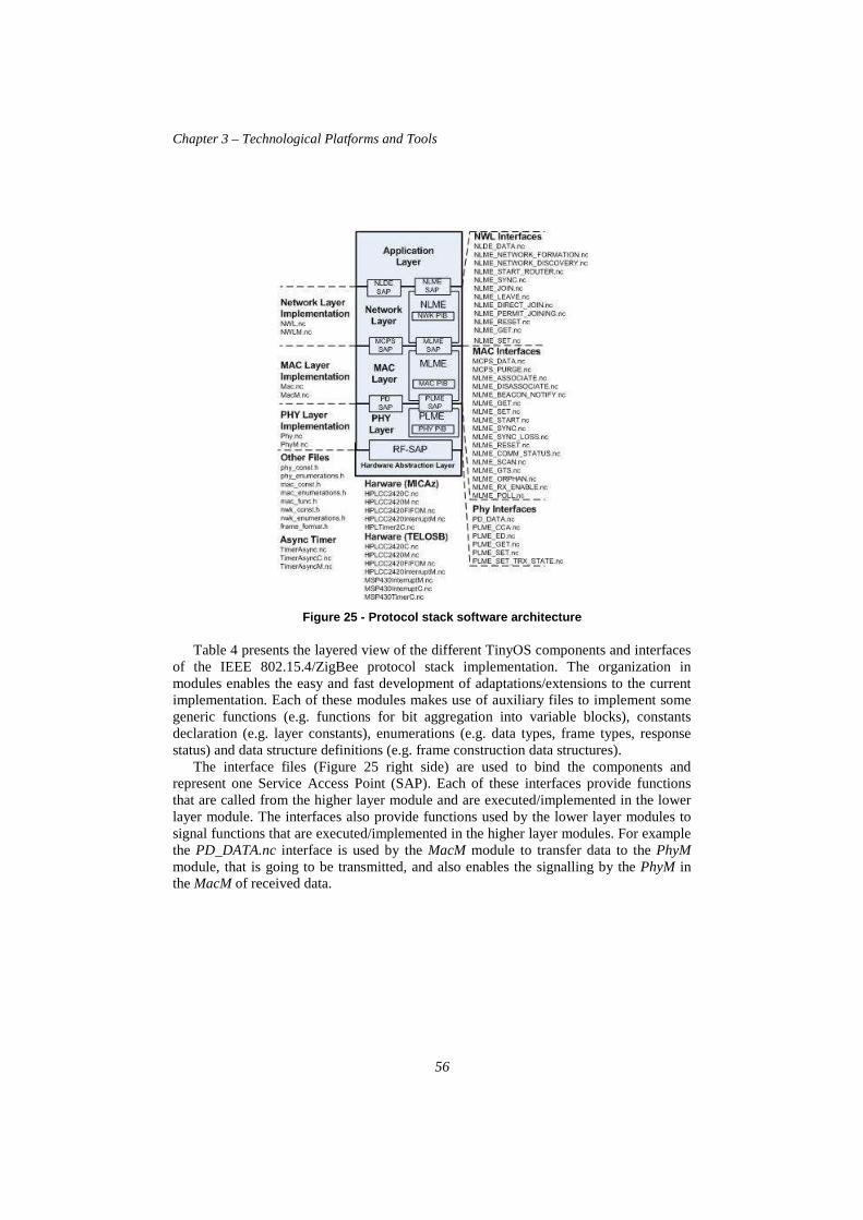
Chapter 3 – Technological Platforms and Tools
56
Figure 25 - Protocol stack software architecture
Table 4 presents the layered view of the different TinyOS components and interfaces of the IEEE 802.15.4/ZigBee protocol stack implementation. The organization in modules enables the easy and fast development of adaptations/extensions to the current implementation. Each of these modules makes use of auxiliary files to implement some generic functions (e.g. functions for bit aggregation into variable blocks), constants declaration (e.g. layer constants), enumerations (e.g. data types, frame types, response status) and data structure definitions (e.g. frame construction data structures).
The interface files (Figure 25 right side) are used to bind the components and represent one Service Access Point (SAP). Each of these interfaces provide functions that are called from the higher layer module and are executed/implemented in the lower layer module. The interfaces also provide functions used by the lower layer modules to signal functions that are executed/implemented in the higher layer modules. For example the PD_DATA.nc interface is used by the MacM module to transfer data to the PhyM module, that is going to be transmitted, and also enables the signalling by the PhyM in the MacM of received data.

Chapter 3 – Technological Platforms and Tools
57
Table 4 - Functionalities of the implemented protoc ol stack components [62]
Component Functionalities
PHY
Activation and deactivation of the radio transceiver; Energy detection within the current channel; Transceiver data management, Received Signal Strength Indication (RSSI) readings and channel frequency selection; Clear Channel Assessment (CCA) procedure for the CSMA/CA mechanism; Data transmission and reception management.
MAC
Beacon generation if the device is a Coordinator; Synchronization services; PAN association and disassociation procedures; CSMA/CA as a contention access mechanism; GTS management mechanism.
NWL
Definition of the network topology (by enabling the device operation as a ZC, ZR or ZED); Association mechanisms; ZigBee addressing schemes; Maintenance of neighbour tables; Tree-Touting.
Figure 26 depicts the relations between different components of the IEEE
802.15.4/ZigBee protocol stack implementation. Note that some components used in our IEEE 802.15.4/ZigBee protocol stack implementation are already part of the TinyOS operating system, namely the hardware components (e.g. the HPL<…>.nc and the MSP430<…>.nc modules).
Figure 26 - TinyOS implementation diagram [62]

Chapter 3 – Technological Platforms and Tools
58
In this implementation, there is no direct interaction with the hardware. In fact, TinyOS already provides hardware drivers forging a hardware abstraction layer used by the Phy component. In Figure 26, observe that the components filled in white are hardware components already provided by the TinyOS operating system.
Refer to an extended implementation technical report in [62] for a detailed description of the implementation functions, variables and protocol mechanisms.
3.6.2 The Open-ZB IEEE 802.15.4 Simulation Model The OPNET Modeler [42] is an industry discrete-event network modelling and simulation environment. It includes libraries of networking technologies and communication protocols, such as the Transmission Control Protocol / Internet Protocol (TCP/IP), hypertext transfer protocol (HTTP), open shortest path first routing (OSPF), asynchronous transfer mode (ATM), frame relay, IP-QoS, 802.11, or Wi-Fi, and 802.16, or even WiMAX. These libraries provide the building blocks used to generate models of networks. One of the several add-on modules available from OPNET is the wireless module. It extends the functionality of the OPNET Modeler with modelling, simulation and analysis of wireless networks. Our simulation model [65] builds on the wireless module, an add-on that extends the functionality of the OPNET Modeler with accurate modelling, simulation and analysis of wireless networks. The simulation model implements physical and medium access control layers defined in the IEEE 802.15.4-2003 standard. The OPNET Modeler is used for developing, namely due to its accuracy and to its sophisticated graphical user interface.
The actual version of the simulation model only supports the star topology where the communication is established between devices, called inside the model End Devices, and a single central controller, called PAN Coordinator. Each device operates in the network must have a unique address.
There are two types of nodes inside the simulation model:
− wpan_analyzer_node: This node captures global statistical data from whole PAN (one within PAN).
− wpan_sensor_node: This node implements the IEEE 802.15.4-2003 standard as was mentioned above.
The structure of the IEEE 802.15.4 sensor nodes (wpan_sensor_node) used in the
simulation model is composed of four functional blocks (Figure 27): 1. The Physical Layer consists of a wireless radio transmitter (tx) and receiver
(rx) compliant to the IEEE 802.15.4 specification, operating at the 2.4 GHz frequency band and a data rate equal to 250 kbps. The transmission power is set to 1 mW and the modulation technique is Quadrature Phase Shift Keying (QPSK).
2. The MAC Layer implements the slotted CSMA/CA and GTS mechanisms. The GTS data traffic (i.e. time-critical traffic) incoming from the application layer is stored in a buffer with a specified capacity and dispatched to the network when the corresponding GTS is active. The non time-critical data frames are stored in an unbounded buffer and based on the slotted CSMA/CA algorithm are transmitted to the network during the active CAP. This layer is also responsible

Chapter 3 – Technological Platforms and Tools
59
for generating beacon frames and synchronizing the network when a given node acts as PAN Coordinator.
3. The Application Layer consists of two data traffic generators (i.e. Traffic Source and GTS Traffic Source) and one Traffic Sink. The Traffic Source generates unacknowledged and acknowledged data frames transmitted during the CAP (uses slotted CSMA/CA). The GTS Traffic Source can produce unacknowledged or acknowledged time-critical data frames using the GTS mechanism. The Traffic Sink module receives frames forwarded from lower layers and performs the network statistics.
4. The Battery Module computes the consumed and the remaining energy levels. The default values of the current draws are set to those of the MICAz mote specification [25].
Figure 27 - The IEEE 802.15.4 [65]
The actual version of the simulation model is 2.0 and is not backward-compatible to the previous version 1.0, meaning that the devices conforming to version 1.0 are not capable of joining and functioning in a PAN composed of devices conforming to version 2.0 and vice-versa. The actual version 2.0 of the simulation model implements the following functions in accordance with the IEEE 802.15.4-2003 standard. Supported (implemented) features:
− Beacon-enabled mode − Slotted CSMA/CA MAC protocol − Frame formats (beacon, command, ack, mac_packet) − Physical layer characteristics − Computation of the power consumption (MICAz and TelosB (TmoteSky)
motes supported) - Battery Module
idlewait_beaconinit gts_slot
init_backoff
backoff_timerCCA
MAC Process Model
The slotted CSMA/CA mechanism
(GTS_STOP)
(PACKET_READY_TO_SEND)(CCA_END)/queue_status()
(DEAFAULT_INTRPT)/queue_status()
(default) (default)
(default)
(default)
(BACKOFF_EXPIRED && CAP_IS_ACTIVE)/wpan_cca_defer()
(GTS_START)/wpan_gts_slot_init()
(CHANNEL_BUSY)/wpan_backoff_update()
init idle
generate
stop
(PACKET_GENERATE)
(STOP)
(default)
GTS Traffic Source Process Model
(default)
(BACKOFF_EXPIRED && !CAP_IS_ACTIVE)/cap_is_not_active()
Sensor Node Model APPLICATION LAYER
MAC LAYER
PHYSICAL LAYER
Battery
Traffic Sink Traffic Source
UNACKPACKETS
ACKPACKETS
Synchro wpan_mac
tx rx
GTSTraffic Source
(default)
GTS Permit
User Defined Attributes
Start Time (seconds)Stop Time (seconds)Length (slots)DirectionBuffer Capacity (bits)
MSDU Interarrival TimeMSDU Size (bites)Acknowledgement
Traffic Source
GTS SettingGTSLoggingIEEE 802-15-4BatteryCSMA/CA ParametersTraffic Source
namemodel
SENSOR NODE

Chapter 3 – Technological Platforms and Tools
60
− Guaranteed Time Slot (GTS) mechanism (GTS allocation, deallocation and reallocation functions)
− Generation of the acknowledged and unacknowledged application data (MAC Frame payload = MSDU) transmitted during the Contention Access period (CAP)
− Generation of the acknowledged or unacknowledged application data transmitted during the Contention Free Period (CFP)
Non-supported features:
− Non beacon-enabled mode − Unslotted CSMA/CA MAC protocol − PAN management (association/disassociation) − ZigBee Network Layer − The values of all constants and variables in this simulation model are
considered for the 2.4 GHz frequency band with a data rate of 250 kbps, which is supported by the MICAz or TelosB motes, for example. In this case, one symbol corresponds to 4 bits. For other frequency bands and data rates it is necessary to change appropriate parameters inside the simulation model (e.g. the header file wpan_params.h).
For more details about the Open-ZB OPNET simulation model, please refer to the
technical report in [65].

Chapter 4 On the Performance Evaluation of the IEEE
802.15.4 Slotted CSMA/CA Mechanism
This chapter addresses the performance evaluation of the Slotted CSMA/CA mechanism, both through an experimental testbed and through simulation. The analysis tries to assess the impact of the choice of Beacon Order (BO) and Backoff Exponent (BE), in the network performance, based in known metrics like the Probability of Successful Transmissions and Network Throughput as a function of the Offered Load.
4.1 Introduction The IEEE 802.15.4 Slotted CSMA/CA mechanism was evaluated with the purpose of measuring its performance and the effectiveness of the available hardware platforms. Moreover, this analysis permits to identify the mechanism limitations and may trigger the proposal of improved schemes for specific purposes (e.g. reducing average delays, improving the throughput).
The analysis was done for different network settings, in order to understand the impact of some protocol parameters on the network performance, namely in terms of Network Throughput (S) and Probability of Successful transmissions (Ps), given a certain Offered Load (G). These performance metrics are based on an extensive study of the Slotted CSMA/CA presented in [63].
The performance metrics analyzed in this work are the following. − Network Throughput (S). It is the fraction of traffic correctly received by the
Network Analyzer, normalized by the network capacity of the IEEE 802.14.5 Physical Layer (250 kbps). The S(G) analysis of CSMA-like mechanisms was first introduced in [64].

Chapter 4 – On the Performance Evaluation of the IEEE 802.15.4 Slotted CSMA/CA Mechanism
62
− Success probability (Ps). This metric is computed as S divided by Gmac, i.e. Ps = S / Gmac. It reflects the degree of reliability achieved by the network for successful transmissions. We denote by Ps(G) the success probability as a function of the offered load G.
4.2 Experimental and Simulation Testbeds In order to accomplish this evaluation, an OPNET [42] simulation model [65] for the IEEE 802.15.4 supporting the slotted CSMA/CA mechanism was used as a means to compare experimental and simulation results, for the same scenarios.
In general, both the simulation and experimental scenarios consist of 1 PAN Coordinator and ten End Devices generating traffic (data frames with 63 bytes of length) at pre-programmed inter-arrival times (at the Application Layer) and a network/protocol analyzer capturing all the data for later processing and analysis. We assume that the generated data frames have a constant size and are equal in all nodes.
The global offered load (denoted as G) generated by all node's application layers depends on the inter-arrival times, which are exponentially distributed (Poisson arrivals). Basically, the performance of the slotted CSMA/CA mechanism will be evaluated as a function of the offered load G in the network.
The simulation and the experimental scenarios are depicted in Figure 28 and Figure 29, respectively. In Figure 28 is possible to observe the network layout and the attributes of each End Device node (wpan_sensor_node model).
Figure 28 - Simulation Model setup

Chapter 4 – On the Performance Evaluation of the IEEE 802.15.4 Slotted CSMA/CA Mechanism
63
Figure 29 depicts the experimental testbed, using MICAz motes. In general, the hardware testbed consists of one Coordinator, ten end devices, one packet sniffer and one configuration node.
The configuration node consists of a MICAz mote attached to a MIB510 [33] board which provides a serial interface to a computer. This node is used to setup the message inter-arrival times, frame size or any other network parameter of the traffic generating nodes thus providing a way of changing the nodes configuration without the need of reprogramming. This setting is done by simply sending a packet with all the network parameters values embedded in the payload at the beginning of each run, thus enabling the traffic generation of the end devices. In order to do this, a command is typed in the terminal window of a computer connected to the MIB510 serial interface. At that point, the end-devices already synchronized with the coordinator’s beacon, start transmitting data frames. The data frames were embedded with the necessary data in their payload to enable the analysis.
The packet analyser used to capture all the generated packets was the Chipcon CC2420 Packet Analyser [37]. It generates a text file with all the received packets and the corresponding timestamps. A parser application was developed to retrieve the necessary data from the packet’s payload (by parsing the sniffer’s capture file) and export it to a spreadsheet for processing and result analysis.
Figure 29 - The CSMA/CA performance evaluation test bed
Both the simulation and experimentation scenarios conditions are considered identical. Nevertheless, it is reasonable to admit that the experimental results suffer from uncontrollable factors, such as RF interferences, processing limitations and memory constraints. Moreover, TinyOS also imposes some limitations that may impact in the network behaviour since it is not a real-time operating system as described in Chapter 7.

Chapter 4 – On the Performance Evaluation of the IEEE 802.15.4 Slotted CSMA/CA Mechanism
64
4.3 Performance Analysis
4.3.1 BO and SO effect In this section the simulation and the experimental results are presented and briefly analysed.
Setting BO and SO is one of the most important tasks of the PAN Coordinator. By changing the inter-arrival times, it was possible to achieve different traffic loads (G values). Figure 30 presents the results concerning Network Throughput (S) obtained through simulation (Figure 30 (a) ) and from the hardware testbed (Figure 30 (b) ), for different BO=SO settings).
(a) (b)
Figure 30 - Network Throughput for different BO
As expected, with low SO settings we achieve lower Network Throughput. This is due to two factors. First, with lower SO settings the overhead of the beacon frame is much more significant since beacons are more frequent. Second, CCA deference is more frequent, which leads to more collisions at the start of each superframe. Increasing the superframe order above SO = 5 has very little effect in the Network Throughput, since the probability of deference is much lower, thus reducing the amount of collisions and leading to a higher S around 68 %.
An example of the deference problem is illustrated in Figure 31, depicting a case with three nodes with the same superframe configurations.
As depicted in Figure 31, if we consider greater superframe durations, node 3 can start its transmission before nodes 1 and 2 wake up. These latter nodes will then sense the channel busy (since node 3 is transmitting), and thus go to backoff with higher backoff delay value (after increasing BE).
Therefore, the transmission deference problem is going to be more frequent with lower superframe orders, as the interval between superframes is lower. The probability of transmission deference is minimized with higher SO and when the nodes have different SO enabling the transmissions with less challengers trying to access the medium. As presented in Figure 30 (b), the same behaviour was observed with the experimental testbed, however the maximum S achieved was lower than in the simulation results (around 58 %).

Chapter 4 – On the Performance Evaluation of the IEEE 802.15.4 Slotted CSMA/CA Mechanism
65
Figure 31 - Transmission deference problem
Figure 32 (a and b) compares the transmission Success Probability (Ps) and the offered load, for a given superframe order (SO). The results show that the probability of a successful transmission is quite low when offered load increases, and particularly lower for low SO due to the multiple collisions caused by deference as already explained.
(a) (b)
Figure 32 - Probability of Success for different BO
The comparison between simulation and experimental results for two SO settings (SO=7 and SO=1) is presented in Figure 33.

Chapter 4 – On the Performance Evaluation of the IEEE 802.15.4 Slotted CSMA/CA Mechanism
66
Figure 33 - Experimental vs Simulation( BO=SO=7 and BO=SO=1)
Notice, that although the results are similar (the behaviour predicted by the simulation results holds), there is a difference of approx 10% between simulation and experimental throughput results. We believe that this is mainly because the simulation model does not consider the physical constraints of the MICAz mote, especially the processing power, the TinyOS constraints and overheads and the normal interferences of a real wireless medium.
4.3.2 Backoff exponent The backoff exponent (BE) is an important parameter in the backoff algorithm of slotted CSMA/CA. It enables the computation of the random backoff delay before trying to access the channel. The initial value of macMinBE is 3 but can be set in the range of [0, 5]. Setting this value to 0 disables collision avoidance during the first iteration of the algorithm.

Chapter 4 – On the Performance Evaluation of the IEEE 802.15.4 Slotted CSMA/CA Mechanism
67
The purpose of this section is to study the impact of the initialization value macMinBE on network performance. We run the experiments (both in the simulator and in the hardware deployment), for different values of macMinBE - from 0 to 5. For each configuration, we vary the inter-arrival times of the packet generation in each node to have different offered loads with a constant packet size. Each curve corresponding to a given macMinBE is obtained for thirteen or more different inter-arrival times.
As presented in Figure 34 the network throughput depends on the initialization value macMinBE, but, contrarily to what is expected, the network saturation throughput decreases when increasing the macMinBE. However, this does not mean a worse behavior for higher macMinBE. In fact, the macMinBE has an important influence on the amount of traffic sent to the network by the MAC sublayer (Gmac), as it is shown in Figure 35. Figure 35 presents the offered load produced by the MAC sublayer (Gmac) as a function of the offered load of the application layer (G). The remaining part of the traffic is still queued waiting for service or dropped in case of limited buffer sizes like in the case of the hardware testbed.
Figure 34 - Impact of macMinBE value in the Network Throughput
In a small-scale network with only ten nodes, the increase of macMinBE reduces the load effectively transmitted in the network. This is because high backoff delays will cause more wasted backoff periods not used by any of the competing nodes. This is explained by the small number of competing nodes in the network. As it is expected, increasing the backoff delay interval (starting with high macMinBE) results in a better success probability, while avoiding collisions in smallscale WSNs. Most of the traffic sent is correctly received for high macMinBEs.

Chapter 4 – On the Performance Evaluation of the IEEE 802.15.4 Slotted CSMA/CA Mechanism
68
(a) (b)
Figure 35 - Offered Load for different macMinBE values
Again, the amount of traffic sent in the case of the experimental testbed (Figure 35 (b)) is approximately 20% lower than the one represented in simulation (Figure 35 (a)). We believe this is in fact the cause for the lower throughput verified in the previous experiments. The hardware platforms are unable to transmit such a high amount of traffic thus resulting in lower throughputs.
4.4 Concluding remarks Simulation and experimental results allowed observing similar behaviours, which consolidates the consistency of the implemented version of the Slotted CSMA/CA mechanism and of the IEEE 802.15.4 protocol in general.
As it could be expected, the simulation results for Throughtput and Probability of Success are higher that the experimental results. We believe that this is mainly because the simulation model does not consider some of the physical constraints of the MICAz mote, especially the processing power, the internal delays due to TinyOS overheads and the normal interferences of a real wireless medium.
Considering the exemplifying case of the experiment where SO = BO = 7, Figure 33 depicts the Throughput and the Success Probability curves for different network loads. In this figure, it is possible to observe that the simulation and experimental curves have the same behaviour. One of the reasons for a lower performance with lower SO is due to a more probability of transmission deference (e.g. number of frames that were deferred to the next superframe because the device could not send them in the current one). The transmission deference problem is more frequent with lower Superframe Orders (SO) as the Superframe Duration is smaller. Another factor for the lower performance is the overhead of the beacon frame transmission, which is more significant in lower SO values.Regarding the macMinBE setting, it has an important influence on the amount of traffic sent to the network by the MAC sublayer (Gmac). In a small-scale network with only ten nodes, the increase of macMinBE reduces the load effectively transmitted in the network, which has a positive impact on the success probability (S/Gmac) for small-scale WSNs. Therefore, most of the traffic sent is correctly received for high macMinBEs.

Chapter 5 On a Hidden-Node Avoidance Mechanism
This chapter describes H-NAMe, a simple yet efficient distributed mechanism to overcome the hidden-node problem. H-NAMe relies on a grouping strategy that splits each cluster of a WSN into disjoint groups of non-hidden nodes and then scales to multiple clusters via a cluster grouping strategy that guarantees no transmission interference between overlapping clusters. The feasibility of H-NAMe is demonstrated via an experimental test-bed, showing that it increases network throughput and transmission success probability up to twice the values obtained without H-NAMe.
5.1 Introduction The hidden-node problem has been shown to be a major source of Quality-of-Service (QoS) degradation in Wireless Sensor Networks (WSNs) due to factors such as the limited communication range of sensor nodes, link asymmetry and the characteristics of the physical environment. In wireless contention-based Medium Access Control protocols, if two nodes that are not visible to each other transmit to a third node that is visible to the formers, there will be a collision as illustrated in Figure 36 – usually called hidden-node or blind collision.
This problem leads to the degradation of the following three performance metrics.
1. Throughput, which denotes the amount of traffic successfully received by a destination node and that decreases due to additional blind collisions.
2. Energy-efficiency that decreases since each collision causes a new retransmission.
3. Transfer delay, which represents the time duration from the generation of a message until its correct reception by the destination node, and that becomes larger due to the multiple retransmissions of a collided message.

Chapter 5 – On a Hidden-Node Avoidance Mechanism
70
Figure 36 - A hidden-node collision
Figure 37 presents an example obtained with our OPNET [42] simulation model [65] for the IEEE 802.15.4 protocol, just to highlight the negative impact of the hidden-node problem. We considered a star network spanning on a square surface (100x100 m2) with 100 nodes, where traffic generation followed a Poisson distribution. The throughput is shown for different transmission ranges of the nodes. We vary the transmission range of the nodes by setting different receiver sensitivity levels. The degradation of the throughput performance due to hidden-node collisions is clearly noticeable in Figure 37. This is due to the increase of the hidden-node collision probability when decreasing the transmission range.
Figure 37 - Hidden-node impact on network throughpu t
In the literature, several mechanisms have been proposed to resolve or mitigate the impact of the hidden-node problem in wireless networks. A thorough enumeration of these techniques is available at [14].

Chapter 5 – On a Hidden-Node Avoidance Mechanism
71
These techniques can be categorized as follows:
− The busy tone mechanism, [67], [68] and [69]; − RTS/CTS mechanism, [70], [71], [72] and [73]; − Carrier Sense Tuning, [74], [75] and [76]; − Node Grouping [77];
However, to our best knowledge, no effective solution to this problem in WSNs was
proposed so far. This Chapter presents an efficient solution to the hidden-node problem in
synchronized cluster-based WSNs. Our approach is called H-NAMe and is based on a grouping strategy that splits each cluster of a WSN into disjoint groups of non-hidden nodes. It then scales to multiple clusters via a cluster grouping strategy that guarantees no transmission interference between overlapping clusters.
The recently standardized IEEE 802.15.4/ZigBee protocol stack, which is considered as a promising candidate for WSNs (e.g. [66]), supports no hidden-node avoidance mechanism. This leads to a significant QoS degradation as already seen in Figure 37. The resolution of this problem is of paramount importance for improving reliability, throughput and energy-efficiency. In this line, we show the integration of the H-NAMe mechanism in the IEEE 802.15.4/ZigBee protocols, requiring only minor add-ons and ensuring backward compatibility with their standard specifications. We developed an experimental test-bed and carried out a significant number of experiments showing that H-NAMe increases network throughput and transmission success probability up to 100%, against the native IEEE 802.15.4 protocol.
We believe that the integration of the H-NAMe mechanism in IEEE 802.15.4/ZigBee may be relevant in leveraging the use of these protocols in WSNs and in enriching future versions of their specifications.
5.2 The H-NAMe mechanism
5.2.1 System model We consider a multiple cluster wireless network and we assume that in each cluster there is at least one node with bi-directional radio connectivity with all the other cluster nodes (Figure 38). We denote this node as Cluster-Head (CH). At least the CH must support routing capabilities, for guaranteeing total interconnectivity between cluster nodes.
Nodes are assumed to contend for medium access during a Contention Access Period (CAP), using a contention-based MAC (e.g. CSMA family). A synchronization service must exist to assure synchronization services to all network nodes, either in a centralized (e.g. GPS, RF pulse) or distributed fashion (e.g. IEEE 802.11 TSF, ZigBee). We also assume that there is interconnectivity between all network clusters (e.g. mesh or tree-like topology).

Chapter 5 – On a Hidden-Node Avoidance Mechanism
72
Figure 38 - Network model
Note that although our current aim is to use the H-NAMe mechanism in the IEEE 802.15.4/ZigBee protocols, the system model is generic enough to enable the application of H-NAMe to other wireless communication protocols (e.g. IEEE 802.11).
5.2.2 Intra-cluster grouping Initially, all nodes in each cluster share the same CAP, thus are prone to hidden-node collisions. The H-NAMe mechanism subdivides each cluster into node groups (where all nodes have bi-directional connectivity) and assigns a different time window to each group during the CAP. The set of time windows assigned to node group transmissions is defined as Group Access Period (GAP), and must be smaller or equal to the CAP. In this way, nodes belonging to groups can transmit without the risk of hidden-node collisions.
For the intra-cluster grouping mechanism, we start by assuming that there is no interference with adjacent clusters, since that might also instigate hidden-node collisions.
The H-NAMe intra-cluster grouping strategy comprises four steps, presented hereafter and illustrated in Figure 39.

Chapter 5 – On a Hidden-Node Avoidance Mechanism
73
Figure 39 - Intra-cluster grouping mechanism
A message sequence diagram is presented in Figure 40.
Figure 40 - Intra-cluster grouping message sequence chart

Chapter 5 – On a Hidden-Node Avoidance Mechanism
74
Step 1 - Group Join Request Let us consider a node Ni that wants to avoid hidden-node collisions. Node Ni sends a Group-join.request message to its cluster-head CH, using a specific broadcast address referred to as group management address @GM in the destination address field. @GM is defined as an intra-cluster broadcast address, which must be acknowledged by the cluster-head (in contrast to the typical broadcast address). Obviously, the acknowledgment message (ACK) will be received by all cluster nodes, since the cluster-head is assumed to have bi-directional links with all of them. Such an acknowledged broadcast transmission ensures that the broadcasted message is correctly received by all the neighbors of the broadcasting node (recalling that we assume no inter-cluster interference). In fact, if any collision occurs inside the cluster during the transmission of the broadcast message, then the cluster-head CH will certainly be affected by this collision since it is in direct visibility with all nodes in its cluster. If no collision occurs, then the broadcast message will be correctly received by all nodes and acknowledged by the cluster-head. Hence, since the Group-join.request message is sent using the group management address @GM, CH sends back an ACK frame to Ni notifying it of the correct reception of the group join request. On the other side, all cluster nodes in the transmission range of Ni (thus received the Group-join.request message) and that already belong to a group, check if they have Ni already registered as a neighbor node in their Neighbor Table. We assume that the Neighbor Table is created and updated by each node during network set-up and run-time phases. The Neighbor Table stores the addresses of neighbor nodes and the link symmetry information, which specifies if the link with a corresponding neighbor is bi-directional or not. If a node hears the Group-join.request message and does not belong to any group (it is transmitting in the CAP, thus not in the GAP), then it simply ignores the message. On the other hand, if a node Nj is already in a group and hears the join message, then it records the information about Ni in its Neighbor Table, if it is not registered yet, and will update the link symmetry with direction Ni→Nj.
Step Status. At the end of this step, each node in the transmission range of Ni knows that node Ni is asking for joining a group and registers the neighborhood information of Ni. This only ensures a link direction from Ni to this set of nodes. The link symmetry verification is the purpose of the next step.
Step 2 - Neighbor Notification After receiving the ACK frame of its Group-join.request message, node Ni triggers the aGroupRequestTimer timer, during which it waits for neighbor notification messages from its neighbors that heard its request to join a group and that already belong to a group. Choosing the optimal duration of this timer is out of the scope of this Thesis, but it must be large enough to permit all neighbors to send their notification.
During that time period, all nodes that have heard the join request and that already belong to a group must initiate a Neighbor.notify message to inform node Ni that they have heard its request. One option is that a node Nj directly sends the Neighbor.notify message to node Ni with an acknowledgement request. The drawback of this alternative is that node Nj cannot know when its Neighbor.notify message fails to reach Ni (i.e. ACK frame not received), whether the lost message is due a collision or to the non-visibility of Ni. No clear decision can be taken in that case. A better alternative is that node Nj sends
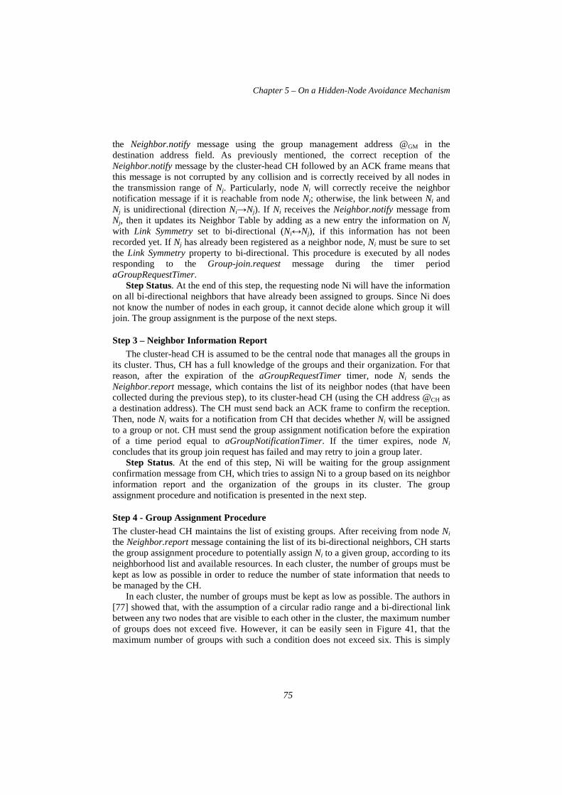
Chapter 5 – On a Hidden-Node Avoidance Mechanism
75
the Neighbor.notify message using the group management address @GM in the destination address field. As previously mentioned, the correct reception of the Neighbor.notify message by the cluster-head CH followed by an ACK frame means that this message is not corrupted by any collision and is correctly received by all nodes in the transmission range of Nj. Particularly, node Ni will correctly receive the neighbor notification message if it is reachable from node Nj; otherwise, the link between Ni and Nj is unidirectional (direction Ni→Nj). If Ni receives the Neighbor.notify message from Nj, then it updates its Neighbor Table by adding as a new entry the information on Nj with Link Symmetry set to bi-directional (Ni↔Nj), if this information has not been recorded yet. If Nj has already been registered as a neighbor node, Ni must be sure to set the Link Symmetry property to bi-directional. This procedure is executed by all nodes responding to the Group-join.request message during the timer period aGroupRequestTimer.
Step Status. At the end of this step, the requesting node Ni will have the information on all bi-directional neighbors that have already been assigned to groups. Since Ni does not know the number of nodes in each group, it cannot decide alone which group it will join. The group assignment is the purpose of the next steps.
Step 3 – Neighbor Information Report The cluster-head CH is assumed to be the central node that manages all the groups in
its cluster. Thus, CH has a full knowledge of the groups and their organization. For that reason, after the expiration of the aGroupRequestTimer timer, node Ni sends the Neighbor.report message, which contains the list of its neighbor nodes (that have been collected during the previous step), to its cluster-head CH (using the CH address @CH as a destination address). The CH must send back an ACK frame to confirm the reception. Then, node Ni waits for a notification from CH that decides whether Ni will be assigned to a group or not. CH must send the group assignment notification before the expiration of a time period equal to aGroupNotificationTimer. If the timer expires, node Ni concludes that its group join request has failed and may retry to join a group later.
Step Status. At the end of this step, Ni will be waiting for the group assignment confirmation message from CH, which tries to assign Ni to a group based on its neighbor information report and the organization of the groups in its cluster. The group assignment procedure and notification is presented in the next step.
Step 4 - Group Assignment Procedure The cluster-head CH maintains the list of existing groups. After receiving from node Ni the Neighbor.report message containing the list of its bi-directional neighbors, CH starts the group assignment procedure to potentially assign Ni to a given group, according to its neighborhood list and available resources. In each cluster, the number of groups must be kept as low as possible in order to reduce the number of state information that needs to be managed by the CH.
In each cluster, the number of groups must be kept as low as possible. The authors in [77] showed that, with the assumption of a circular radio range and a bi-directional link between any two nodes that are visible to each other in the cluster, the maximum number of groups does not exceed five. However, it can be easily seen in Figure 41, that the maximum number of groups with such a condition does not exceed six. This is simply

Chapter 5 – On a Hidden-Node Avoidance Mechanism
76
because the area of the circular range of the cluster head can be decomposed into six equal regions defined by isosceles triangles. The maximum distance between two points into the same region is always lower than or equal to the radius of the circle.
Figure 41 - Maximum number of groups in a cluster a ssuming bi-directional links and circular radio range
Note that without the assumption of a bi-directional link between each couple of nodes inside a cluster, the maximum number of groups cannot be controlled in case of asymmetric links due to the presence of obstacles or different transmission ranges of different nodes in the cluster. Here, we consider the case of asymmetric links since it is more realistic. We impose that the number of groups inside each cluster must not exceed aMaxGroupNumber, which should be equal to six by default. This parameter can be set differently by the cluster head CH.
The group assignment algorithm is presented in Figure 42. Upon reception of the Neighbor.report message, the cluster-head CH checks the neighbor list of the requesting node Ni. If there is a group whose (all) nodes are neighbors of node Ni, then Ni will be associated to that group. The cluster-head runs the following algorithm (as in Fig. 7). For each neighbor node Nj in the list, the cluster-head CH increments Count [group_index (Nj)], which denotes the number of neighbor nodes of Ni that belong to the group of the currently selected neighbor Nj. Note that group_index (Nj) denotes the index of the group of node Nj. If this number is equal to the actual number of nodes of the latter group, it results that all nodes in this group are neighbors of node Ni. Thus, Ni can be assigned to this group since it is visible to all its nodes. If the list of neighbors is run through without satisfying such a condition, the cluster-head CH will create a new group for Ni if the number of groups is lower than aMaxGroupNumber; otherwise, the Group-join.request message of Ni will be considered as failed. So it must transmit during the CAP (not in the GAP), and may retry a new group join request later.
At the end of the group assignment process, CH sends a Group-join.notify message to node Ni to notify it about the result of its group join request.
If the requesting node is assigned a group, then it will be allowed to contend for medium access during the time period reserved for the group, which is called Group Access Period (GAP). This information on the time period allocated to the group is retrieved in the subsequent frames sent by CH.

Chapter 5 – On a Hidden-Node Avoidance Mechanism
77
Group Assignment Algorithm 1 int aMaxGroupNumber; // maximum number of groups
2 in a cluster
3 Type Group;
4 Group G; // list of all groups G[1]..G[aMaxGroupNumber]
5 |G[i]| = number of elements in group G[i]
6 Type Neighbor_List; // {Np .. Nq)= Neighbor List of
7 the requesting Node N
8 int Count [|G[i]|] = {0, 0, .., 0}; // Number of nodes in Neighbor
9 List that belongs to the group G[i]
10 int grp_nbr; // the current number of groups managed by CH
11 // group_index function returns the group index of the node NL[i]
12 function int group_index(Neighbor_List NL, int i)
13 //the group assignment function.
14 int group_assign (Neighbor_List NL, Group G, int grp_nbr) {
15 int res = 0;
16 int index = 0;
17 while ((res = = 0) and (index < |NL|)) {
18 if (++Count[group_index (NL, index)] = =
19 |G[group_index (NL, index++])|)
20 res = group_index (NL, --index); break;
21 }
22 if (res = = 0) { //that means that no group is found
23 if (grp_nbr = = aMaxGroupNumber) return (res)
24 else return (++grp_nbr);
25 }
26 else return (res);
27 }
Figure 42 - Group assignment algorithm
Importantly, the complexity of the algorithm for assigning a group to a node depends on the number of neighbours of this node. In any case, it is smaller than O(N), where N is the number of nodes in the cluster, thus has significantly lower complexity than the O(N²) complexity of the algorithm for group assignment proposed in [77]. Moreover, in that proposal each new node that enters the network is unaware of the existing groups and will cause a hidden-node collision, after which the groups are re-constructed. In our mechanism, a node is not allowed to transmit during the time period allocated to groups (only being able to communicate during the CAP) until it is assigned to a given group.
Group load-balancing: Note that the algorithm presented in Figure 42 stops when a first group of non-hidden nodes is found for the requesting node. However, a requesting node can be in the range of two different groups, i.e. all nodes in two separate groups are visible to the requesting node. In this case, one possible criterion is to insert the requesting node into the group with the smallest number of nodes, for maintaining load-balancing between the different groups. For that purpose, the algorithm should go through all the elements of the neighbour list and determine the list of groups that satisfy the condition in lines 18 and 19 of the algorithm (Figure 42). In this case, if more than

Chapter 5 – On a Hidden-Node Avoidance Mechanism
78
one group satisfies this condition, Ni will be inserted in the group with the smallest number of nodes.
Bandwidth allocation: The time-duration of each group in the GAP can be tuned by the cluster-head to improve the mechanism efficiency. This can be done according to different strategies, namely: (i) evenly for all the node groups; (ii) proportionally to the number of nodes in each group; (iii) proportionally to each group’s traffic requirements. How to perform this assignment is not tackled in this Thesis.
5.2.3 Scaling H-NAMe to multiple-cluster networks Solving the hidden-node problem in multiple-cluster networks involves greater complexity due to inter-cluster interference. The assumption that there is no interference from other clusters made before is no longer valid. Hence, even if non-hidden node groups are formed inside all clusters, there is no guarantee that hidden-node collisions will not occur, since groups in one cluster are unaware of groups in adjacent clusters.
Obviously, the best strategy for completely avoiding the inter-cluster hidden-node problem is to reserve an exclusive time window for each cluster. However, this strategy is definitely not adequate for large-scale sensor networks, where the number of clusters/groups is significantly high.
Our approach consists in defining another level of grouping by creating distinct groups of clusters, whose nodes are allowed to communicate during the same time window. Therefore, each cluster group will be assigned a portion of time, during which each cluster in the cluster group will manage its own Group Access Period (GAP), according to the intra-cluster mechanism presented in Section 5.2.2.
The cluster grouping concept is illustrated in Figure 38. As shown, clusters A and B have overlapping radio coverage, which can lead to inter-cluster interference and thus to hidden-node collisions. For this reason, they will be assigned to different cluster groups that are active in different time windows. The same applies for cluster pairs (C, D), (A, C) and (B, D). Therefore, our cluster grouping mechanism forms two cluster groups: Group 1, which comprises clusters A and D, and Group 2, containing clusters B and C.
The challenge is on finding the optimal cluster grouping strategy that ensures the minimum number of cluster groups. We define a cluster group as a set of clusters whose nodes are allowed to transmit at the same time without interference.
Cluster grouping and time window scheduling strategies were proposed and effectively implemented and validated in [78], for engineering ZigBee cluster-tree WSNs. We propose a grouping criterion and a graph colouring algorithm for an efficient scheduling of the cluster groups activity.
5.3 H-NAMe in IEEE 802.15.4/ZigBee In this section, we explain how to instantiate the H-NAMe mechanism to the IEEE 802.15.4 protocol, namely addressing beacon-enabled cluster-tree networks. This topology is scalable and enables energy-efficient (dynamically adaptable duty-cycles per cluster) and real-time communications. In addition, the cluster-tree topology fits into the H-NAMe network model.
Basically, the idea is that each node group (resulting from the H-NAMe mechanism) will be allocated a time window in each superframe duration. The idea is to use part of the CAP for the Group Access Period (GAP), as illustrated in Figure 43. Note that a

Chapter 5 – On a Hidden-Node Avoidance Mechanism
79
minimum duration of 440 symbols must be guaranteed for the CAP in each superframe [24].
Figure 43 - CAP, GAP and CFP in the Superframe
In our intra-cluster grouping strategy, a node that has been assigned a group will track the beacon frame for information related to the time window allocated to its group, and will contend for medium access during that period with the other nodes of the same group. We propose the GAP Specification field in Figure 44 to be embedded in the beacon frame (such a specification is missing in [77]).
Figure 44 - GAP specification field of a beacon fra me
The GAP is specified by the Group ID field that identifies the node group. Up to 8 groups per cluster can be defined. The time window in the superframe is specified by a given number of Backoff Periods (BP). A practical problem is that the number of a backoff period in a superframe may be quite large for high superframe orders (up to 16 time slots * 216 BP/time slot), which requires a huge amount of bits in the field to express the starting BP and the final BP for each group. The objective is to maintain as low overhead as possible for the specification of a given group. For that purpose, a group is characterized by its start time slot and end time slot (between 0 and 15) and the corresponding backoff period offsets. The start and end offsets for the time duration of a group is computed as follows:
(Start/End) Backoff Period Offset * 2SORelative Offset= The choice of a Backoff Period Offset sub-field encoded in two bits is argued by the
fact that the minimum number of backoff periods in a time slot is equal to 3 for (SO = 0). Hence, for SO > 0, each time slot will be divided into three parts to which the start/end instant of a given group access period should be synchronized.
This GAP implementation approach only requires two bytes of overhead per group. The maximum number of groups depends on the SO values, since lower superframe orders cannot support many overhead in the beacon frame due their short superframe durations. Also, it allows a flexible and dynamic allocation of the groups, since all nodes continuously update their information about their group start and end times when receiving a beacon frame, at the beginning of each superframe.

Chapter 5 – On a Hidden-Node Avoidance Mechanism
80
5.4 Experimental Evaluation
5.4.1 Implementation approach We have implemented the H-NAMe mechanism in nesC/TinyOS [43], over the Open-ZB implementation [62] of the IEEE 802.15.4/ZigBee protocols, to demonstrate its feasibility and efficiency using commercial-off-the-shelf (COTS) technologies.
For that purpose, we carried out a thorough experimental analysis to understand the impact of the H-NAMe mechanism on the network performance, namely in terms of network throughput (S) and probability of successful transmissions (Ps), for different offered loads (G), in one cluster with a star-based topology. Both metrics have been also used to evaluate the performance of the Slotted CSMA/CA MAC protocol in Chapter 4. The network throughput (S) represents the fraction of traffic correctly received normalized to the overall capacity of the network (250 kbps). The success probability (Ps) reflects the degree of reliability achieved by the network for successful transmissions. This metric is computed as the throughput S divided by G, representing the amount of traffic sent from the application layer to the MAC sub-layer, also normalized to the overall network capacity.
To have a clearer idea on the impact of the hidden-node phenomenon independently from other parameters, we have chosen a superframe order sufficiently high (SO = 8) to avoid the collisions related to the CCA deference problem encountered for low SO, in the slotted CSMA-CA mechanism, as presented in [63] and in Chapter 4 of this Thesis. The CCA deference problem occurs when it is not possible for a frame to be transmitted in the remaining space of the superframe and its transmission must be deferred to the next one. For low SO and due to the lower superframe duration, it is more probable that this deference occurs (in more nodes), resulting in multiple collisions at the beginning of the next superframe. The reason is that, after the deference, the slotted CSMA-CA protocol does not perform another backoff procedure (only two CCAs).
5.4.2 Test-bed scenario The experimental test-bed consisted of 18 MICAz motes [25] (featuring an Atmel ATmega128L 8-bit microcontroller with 128 kB of in-system programmable memory) scattered in three groups hidden from each other, a ZC and a protocol analyzer Chipcon CC2420 [37], capturing the traffic for processing and analysis (Figure 45).
The protocol analyzer generates a log file containing all the received packets and the corresponding timestamps, enabling to retrieve all the necessary data embedded in the packets payload, using a parser application we developed, presented in Chapter 4.
The 18 nodes have been programmed to generate traffic at the application layer with preset inter-arrival times. A similar approach has previously been used in Chapter 4, for evaluating the performance of the CSMA-CA protocol. The three node groups were placed at ground level near walls, in order to reinforce the hidden-node effect (Figure 45). To ensure that nodes in different groups were in fact hidden, a simple test was carried out.

Chapter 5 – On a Hidden-Node Avoidance Mechanism
81
Figure 45 - Experimental testbed
A MICAz mote was programmed to continuously perform the clear channel assessment procedure, toggling a led when energy was detected in the channel. By placing this mote at different spots while a group of nodes was transmitting, we were able to identify an area to place a new node group so that they would be hidden from the other groups. This procedure was repeated for each group, in a way that nodes were divided evenly by the 3 groups (6 nodes/group).
5.4.3 Experimental results Figure 46 presents the GAP created by the H-NAMe mechanism.
Figure 46 - Groups allocation in the superframe
Each node group was assigned with four time slots for transmission, which represents a theoretical duration of 983.04 ms per group (SO = 8). This allocation was made according to the principle of equal group access duration for an equal number of nodes per group.
5.4.4 The node group-join procedure
Figure 47 illustrates a packet capture of a group join requested by a node. In this example, a node with short address 0x0006 (see Figure 47) requested to join a group. Notice the beacon payload featuring the GAP specification of the groups already formed (labeled (1) in Figure 47).

Chapter 5 – On a Hidden-Node Avoidance Mechanism
82
The node initiated the process by sending a Group-join.request message to the ZC (label (2)) and receiving an acknowledgement. Then, all the other nodes in its transmission range replied with a Neighbor.notify message (label (3)). When the requesting node receives these messages, it knows that it shares a bi-directional link with its neighbors. As soon as the timer for receiving Neighbor.notify messages expires, the requesting node sends a Neighbor.report message to the ZC identifying its neighbors (label (4)). The ZC runs the H-NAMe intra-cluster grouping algorithm to assign a group to that node and sends a Group-join.confirm message, notifying the node of which group to join (label (5)). The node, now assigned to Group 1, can transmit during the GAP portion reserved for Group 1 (see Figure 46).
Figure 47 - Packet analyzer capture of a group join
5.4.5 H-NAMe performance evaluation The performance evaluation of the H-NAMe mechanism has been carried out using BO = SO = 8 (100% duty cycle), with a constant frame size of 904 bits. Several runs were
(1)
(5)
(2)
(3)
(4)
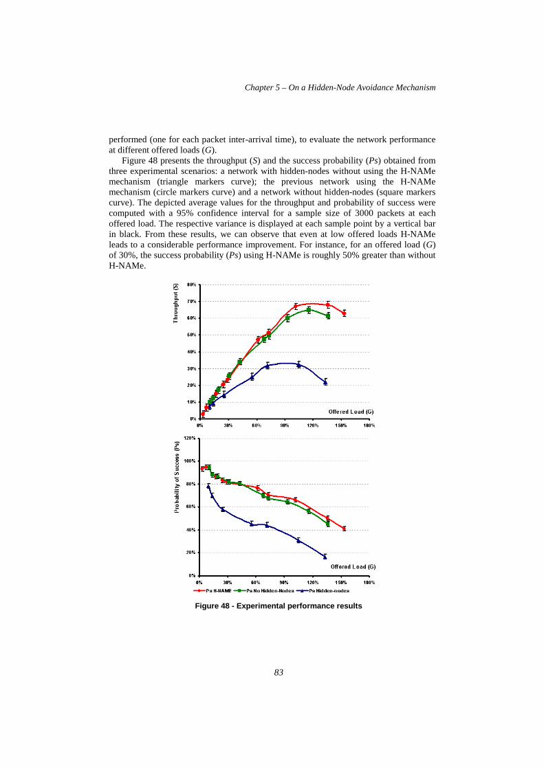
performed (one for each packet interat different offered loads (
Figure 48 presents the throughput (three experimental scenarios: a network with hiddenmechanism (triangle markers curve); the previous netwmechanism (circle markers curve) and a network without hiddencurve). The depicted average values for the throughput and probability of success were computed with a 95% confidence interval for a sample size of 300offered load. The respective variance is displayed at each sample point by a vertical bar in black. From these results, we can observe that even at low offered loads Hleads to a considerable performance improvement. For instance, foof 30%, the success probability (H-NAMe.
Figure
Chapter 5 – On a Hidden-Node Avoidance Mechanism
83
performed (one for each packet inter-arrival time), to evaluate the network performance at different offered loads (G).
presents the throughput (S) and the success probability (Ps) obtained from three experimental scenarios: a network with hidden-nodes without using the Hmechanism (triangle markers curve); the previous network using the Hmechanism (circle markers curve) and a network without hidden-nodes (square markers curve). The depicted average values for the throughput and probability of success were computed with a 95% confidence interval for a sample size of 3000 packets at each offered load. The respective variance is displayed at each sample point by a vertical bar in black. From these results, we can observe that even at low offered loads Hleads to a considerable performance improvement. For instance, for an offered load (of 30%, the success probability (Ps) using H-NAMe is roughly 50% greater than without
Figure 48 - Experimental performance results
Node Avoidance Mechanism
arrival time), to evaluate the network performance
) obtained from nodes without using the H-NAMe
ork using the H-NAMe nodes (square markers
curve). The depicted average values for the throughput and probability of success were 0 packets at each
offered load. The respective variance is displayed at each sample point by a vertical bar in black. From these results, we can observe that even at low offered loads H-NAMe
r an offered load (G) NAMe is roughly 50% greater than without

Chapter 5 – On a Hidden-Node Avoidance Mechanism
84
Considering higher loads, it is clear that the H-NAMe doubled the throughput of the conventional network with hidden-nodes. At 90% of offered load (G), the throughput of the network using H-NAMe reached 67% and is increasing, while without using H-NAMe a saturation throughput of 32% is achieved, representing an improvement of more than 100%.
Moreover, it is possible to observe that for high offered loads, the H-NAMe mechanism has actually up to 5% better throughput performance than that of a network without hidden-nodes. This results from the lower probability of collisions with H-NAMe since at most 6 nodes (one group) contend for the medium at a given time (GAP) instead of 18 nodes in the network without H-NAMe intra-cluster grouping.
In this experimental scenario, there were no packets retransmitted (due to collisions). However, if we consider one retransmission for each lost packet, the increase in the number of transmissions would be significant in the case of the network without H-NAMe, thus leading to a much higher energy loss, even at low offered loads. Notice that for G = 30%, Ps is around 50% when H-NAMe is not used, meaning that half of the packets transmitted did not reach their destination.
In conclusion, it can be noticed that the H-NAMe mechanism presents a significant improvement of the network performance in terms of throughput and success probability, at the small cost of some additional overhead to setup the different groups in the networks.
5.5 Concluding remarks In this chapter, we have described a solution to a real fundamental problem in Wireless Sensor Networks (WSNs) that use contention-based medium access control (MAC) – the hidden-node problem.
We have proposed a simple yet very effective mechanism – H-NAMe – that eliminates hidden-node collisions in synchronized multiple cluster WSNs, leading to improved network throughput, energy-efficiency and message transfer delays. H-NAMe follows a proactive approach (avoids hidden-node collisions before occurring) for achieving interference-free node and cluster groups.
We have also showed how H-NAMe can easily be applied to the IEEE 802.15.4/ZigBee protocols, which are prominent candidates for WSN applications. Finally, we have implemented, tested, validated and demonstrated the feasibility and effectiveness of the H-NAMe mechanism in a real scenario, reaching a network performance improvement at the order of 100%.

Chapter 6 Real-Time Communications over Cluster-Tree
Wireless Sensor Networks
Modelling the fundamental performance limits of Wireless Sensor Networks (WSNs) is of paramount importance to understand the behaviour of WSN under worst-case conditions and to make the appropriate design choices. This chapter focuses on the experimental test and validation of a methodology for modelling cluster-tree WSNs where the sink can be static or mobile. Worst-case end-to-end delays, buffering and bandwidth requirements across any source-destination path in the network are compared to the experimental (maximum, average) results.
6.1 Introduction Wireless Sensor Networks (WSNs) emerge as enabling infrastructures for large-scale distributed embedded systems. Timeliness is an important requirement to be fulfilled in these systems. However, issues such as large scale and communication, computing and energy limitations pose important difficulties in guaranteeing a correct behaviour of these systems.
Evaluating the performance limits of WSNs is therefore a crucial task, particularly when the network is expected to operate under worst-case conditions [80], [81]. For achieving real-time communications over sensor networks, it is mandatory to rely on deterministic routing and MAC (Medium Access Control) protocols. Usually, these networks use hierarchical logical topologies such as cluster-tree or hexagonal (e.g. [82], [83]). Issues such as the use of contention-free MAC protocols (e.g. time division or token passing) and the possibility of performing end-to-end resource reservation contrast with what can be achieved in mesh-like topologies, where contention-based MACs and probabilistic routing protocols are used.

Chapter 6 – Real-Time Communications over Cluster-Tree Wireless Sensor Networks
86
In a previous work [79], the authors have provided a methodology and closed-form expressions to dimension the network resources in a cluster-tree WSN with a static sink. The sink – a central point that collects all sensory data – was assumed to be statically attached to the root. That work aimed at evaluating the worst-case network performance assuming a cluster-tree topology of balanced height and load. This symmetry property was explored to derive per-hop and end-to-end resource requirements in addition to the worst-case delays of upstream flows (i.e. from child nodes to the root).
However, while the static sink behaviour is adequate for root-centric WSN applications (e.g. a surveillance system delivering alarms to a central station), other applications may impose or benefit from collecting data at different network locations (e.g. a doctor with a hand-held computer collecting patients’ status).
This chapter presents the experimental validation of a theoretical model that permit the worst-case dimensioning and analysis of cluster-tree WSNs, based in Network Calculus, by comparing worst-case results (buffer requirements and message end-to-end delays) with the maximum and average values measured through an experimental test-bed based on real COTS technologies.
6.2 Background on Network Calculus Network Calculus [84] is a mathematical methodology based on min-plus algebra that applies to the deterministic analysis of queuing/flows in the networks. This section briefly introduces the aspects that are most significant to this work. For additional details please refer to [84].
A basic system model S in Network Calculus consists of a buffered FIFO node with the corresponding transmission link (Figure 49).
Figure 49 -The basic system model of Network Calcul us
For a given data flow, the input function R(t) is a cumulative number of bits that have arrived to system S in the time interval (0, t). The output function R*(t) is the number of bits that have left S in the same interval (0, t). An arrival curve α (t) upper bounds the input function of a system S such that for ∀s, 0 ≤ s ≤ t, R(t) - R(s) ≤ α (t - s). A service curve β (t) represents a lower bound on the transmitted cumulated flow, thus for ∀t there exists t0 ≤ t such that R*(t) - R*(t0) ≥ β (t -t0). The knowledge of the arrival and service curves enables us to determine performance bounds, namely the delay bound Dmax given by the maximum horizontal distance between α (t) and β (t), which represents the worst-case delay of the message traversing system S, and the backlog bound Qmax given by the maximum vertical distance between α (t) and β (t), which represents the minimum buffer size requires inside S. These concepts are illustrated in Figure 50.

Chapter 6 – Real-Time Communications over Cluster-Tree Wireless Sensor Networks
87
Figure 50 - Example of input R(t) and output R*(t) functions constrained by (b, r) arrival curve α(t) and rate-latency service curve β(t), respectively.
So far, we have handled a system S as a single buffered node. However, system S might be also a sequence of nodes or even a complete network. If so, the concatenation theorem enables to investigate systems in sequence as a single system. This theorem is described in more detail in [16].
The accuracy of the worst-case bounds depends on how tightly the selected arrival and service curves follow the real network behaviour. Different types of arrival and service curves have been proposed in Network Calculus . However, the (b, r) arrival curve and rate-latency service curve are the most used in such network models. The (b, r) arrival curve is defined as α (t) = b + r·t for ∀t > 0, where b is called burst tolerance, which is the maximum number of bits that can arrive simultaneously at a given time to the system S and r is the average data rate. The rate-latency service curve is defined as βR,T (t) = R·(t-T)+, where R ≥ r is the guaranteed link bandwidth, T is the maximum latency of the service, and (x)+ = max(0, x). These curves lead to a fair trade-off between computing complexity and approximation accuracy of the real system behaviour, as it will be seen throughout the rest of the paper.
Hereafter, we consider a data flow constrained by the (b, r) arrival curve α (t) and traversing system S with a rate-latency service curve βR,T (t). Then, the guaranteed performance bounds Dmax and Qmax (see Figure 50 for additional intuition) are easily computed as:
���� = �� +
��� = � + � ∙ (6.1)
6.3 System Model This section defines the cluster-tree topology and data flow models that will be considered in the analysis. It also elaborates on the worst-case cluster scheduling; that is, the time sequence of clusters’ active periods leading to the worst-case end-to-end delay for a message to be routed to the sink.
arrival curve
α(t) = b+rt
α*(t) = (b
+rT)+rt

Chapter 6 – Real-Time Communications over Cluster-Tree Wireless Sensor Networks
88
6.3.1 Cluster-tree topology model Cluster-tree WSNs feature a tree-based logical topology, where nodes are organized in different groups, called clusters. Each node is connected with one node at lower depth, called parent node, and can be connected with multiple nodes at upper depth, called child nodes.
The cluster-tree topology contains two main types of nodes. First, the nodes that can associate with previously associated nodes and can participate in the multi-hop routing are referred to as routers (Rij, i.e router j at depth i). Second, the leaf nodes that do not allow association of other nodes and do not participate in routing are referred to as end-nodes (N). The router that has no parent is called root (it might hold special functions such as identification, formation and control of the entire topology). Routers and end-nodes can both have sensing capabilities. Therefore they are generally referred to as sensor nodes. Each router forms its cluster and is referred to as cluster-head of this cluster.
In this work we aim at specifying the worst-case cluster-tree topology, i.e. the network topology configuration that leads to the worst-case performance. This means that a dynamically changing cluster-tree WSN can assume different configurations, but it can never exceed the worst-case topology, in terms of maximum depth and number of child routers/end-nodes. Thus, the worst-case cluster-tree topology is graphically represented by a rooted balanced directed tree [85] defined by the following three parameters:
− : Height of the tree, i.e. the maximum number of logical hops from the deepest router to the root. A tree with only a root has a height of zero.
− ����_������� : Maximum number of end-nodes that can be associated to a router. − ���������� : Maximum number of child routers that can be associated to a parent
router.
The depth of a node is defined as the number of logical hops from that node to the root. The root is at depth zero, and the maximum depth of an end-node is H+1.
Note that the sink is a special type of node that gathers the sensory data from all sensor nodes inside the network. Unlike previous work, we relax the assumption that the sink is only associated with the root and consider the sink to be an autonomous and topology-independent mobile node. The mobile behaviour means that a sink moves arbitrarily within a static cluster-tree WSN and can be associated with any router within communication range. The router, to which the sink is in a given moment associated, is referred to as sink router. There can be more than one mobile sink in a WSN, but we assume that only one is active (i.e. gathers the sensory data) at a given time. We specify another parameter, ����� ∈ 0, �#, to represent the depth at a given moment of the sink router in a cluster-tree topology. Note that if the sink is associated with the root, i.e. ����� = 0, the network contains only upstream flows. This case has already been analysed in [79]. In this work, we analyze the case where ����� > 0.

Chapter 6 – Real-Time Communications over Cluster-Tree Wireless Sensor Networks
89
Figure 51 - The cluster-tree topology and data flow models
Our terminology and conventions are as illustrated in Figure 51, corresponding to a configuration where � = 2, '(�)_�*)(+,- = 3, '/*01(/+,- = 2, and ����� = 2. Note that a cluster-tree WSN may contain additional nodes per router than those defined by '/*01(/+,- and '(�)_�*)(+,- parameters. However, these additional nodes cannot be granted guaranteed resources.
6.3.2 Data Flow Model In this work, we assume that all sensory data is exclusively sent to the sink. All sensor nodes are assumed to sense and transmit data upper bounded by the arrival curve 2)�1� 3# = �)�1� + �)�1� ∙ 3. In case of different data flows, 2)�1� 3# is considered to represent the upper bound of the highest flow in a network. This may introduce some pessimism to the analysis if the variance between data flows is significant.
Each end-node is granted a service guarantee from its parent router corresponding to the rate-latency service curve 4)�1� 3# = �)�1� ∙ 3 − )�1�#6.
The output arrival curve 2)�1�∗ 3#, which upper bounds the outgoing data flow from any end-node is characterized as follows:
2)�1�∗ 3# = 2)�1� 3# + �)�1� ∙ )�1� (6.2)
The computation is showed in [16]. On the other hand, the amount of bandwidth allocated by each router depends on the cumulative amount of data at its inputs, which increases towards the sink. Thus, the total input function R of each router depends on the depth, and consists of the sum of the output functions R* of its end-nodes and child routers. Additionally, the router itself can be equipped with sensing capability producing
β1U
α2U
α1U
β0U
β 0D
α 0D
β dataα data
β1D
α1D
Chapter 6 – Real-Time Communications over Cluster-Tree Wireless Sensor Networks
90
a traffic bounded by 2)�1� 3#. Thus, the arrival curve constraining the total input function R of a router at general depth i is expressed as:
28� = 2)�1� + '(�)_�*)(+,- ∙ 2)�1�∗ + 9 2/*01(/ �6:,;#∗<=>?@A=BCD
;E: (6.3)
The outgoing flow of a router at depth i is upper bounded by the output arrival curve as follows:
2�∗ = 28�⨀4�G: (6.4)
Hence, the data flow analysis consists in the computation of the arrival curves 28� and 2�∗, using iteratively Eqs. (6.3) and (6.4) from the deepest routers until reaching the sink. After that, the resource requirements of each router, in terms of buffer requirement Qi and bandwidth requirement Ri, and the worst-case end-to-end delay bound of WSN are computed.
In cluster-tree WSNs where the sink can be associated with a router other than the root, data flows may then be redirected in the downstream directions. Data flows over upstream links (called upstream flows) have already been analysed in [79]. Data flows over downstream links (called downstream flows), where data is sent from a parent router to its child router, are analysed in this work. In what follows, the upstream and downstream flows are marked by the subscripts U and D, respectively (e.g. 2�H∗ , 2�I∗ ). We also assume two types of service curves (i.e. 4�H for upstream flows and 4�I downstream flows) provided by each parent router at depth i to its child routers at depth i+1, as presented in [16].
To ensure the symmetry properties of the worst-case cluster-tree topology assumed in our methodology, the same downstream or upstream service curves must be guaranteed to all downstream or upstream flows at a given depth, respectively.
The detailed data flow analysis (input and output, upstream and downstream), is presented in [16], along with the worst-case network dimensioning. These methodologies were then applied to the specific case of IEEE 802.15.4/ZigBee.
6.3.3 Time Division Cluster Scheduling In general, the radio channel is a shared communication medium where more than one node can transmit at the same time. In cluster-tree WSNs, messages are forwarded from cluster to cluster until reaching the sink. The time period of each cluster is periodically divided into an active period (AP), during which the cluster-head enables data transmissions inside its cluster, and a subsequent inactive period, during which all cluster nodes may enter low-power mode to save energy resources. To avoid collisions between multiple clusters, it is mandatory to schedule active periods of different clusters in an ordered sequence, called Time Division Cluster Schedule (TDCS). In other words, TDCS is equivalent to a permutation of active periods of all clusters in a WSN such that no inter-cluster interference occurs. In case of one collision domain (i.e. all nodes hear each other), the TDCS must be non-overlapping, i.e. only one cluster can be active at any time. On the contrary, in a network with multiple collision domains, the clusters from different non-overlapping collision domains may be active at the same time. The number of feasible TDCSs in a network with n routers inside one collision domain is equal to the number of permutations given by n factorial (n!). Note that for each data

Chapter 6 – Real-Time Communications over Cluster-Tree Wireless Sensor Networks
91
flow originated in a given node, there is a corresponding best-case/worst-case TDCS that minimizes/maximizes the end-to-end delay of that flow, respectively. Thus, it is impossible to determine a general best-case or worst-case TDCS meeting the requirements of all data flows. Our methodology based on the symmetric properties of cluster-tree topology, for dimensioning the network resources of a WSN for the worst-case TDCS, is presented in more detail in [78].
6.4 IEEE 802.15.4/ZigBee Cluster-Tree WSN Setup For our experimental scenario, we consider a simple cluster-tree WSN corresponding to the configuration where � = 2, '(�)_�*)(+,- = 1, '/*01(/+,- = 2. For the sake of simplicity, only end-nodes are equipped with sensing capability (i.e. S = 0) and generate data flows bounded by the arrival curve 2)�1� 3#. We assume a minimum possible value of SO (e.g. SO = 4, imposed by some technological limitation of our experimental platforms, namely due to the non-preemptive behaviour of the TinyOS [43] operating system. According to [16] the total number of routers is equal to 7. Hence, BO must be set such that at least 7 SDs with SO = 4 can fit inside the BI without overlapping as presented in [16].
As a result for SO = 4, the minimum BO is equal to 7, such that a maximum of 27/24 = 8 SDs can fit in one BI. The maximum duty cycle of each cluster is then equal to (1/8) = 12.5 %. Note that to maximize the lifetime of a WSN, the lowest duty cycles must be chosen. On the other hand, low duty cycles enlarge end-to-end delays. Hence, long lifetime is in contrast to the fast timing response of a WSN, so a trade-off must be found.
According to [24], the minimum CAP is equal to 7.04 ms, assuming the 2.4 GHz ISM band, which corresponds to 1 time slot with SO = 4. The remaining slots can be allocated for GTSs. Hence, the maximum CFP length is equal to LCFP = 15 time slots. With this constraint, a router cannot reserve more than LCFP time slots for 7 GTSs maximum, i.e. for its '(�)_�*)(+,- end-nodes and '/*01(/+,- child routers. Assuming that each end-node requires allocation of a GTS with ')�1�KL time slots (i.e. rdata ≤ ')�1�KL ·RTS) from its parent router. Then, each child router can allocate a GTS with the maximum number of time slots equal to:
MNOPQR − ')�1�KL ∙ '(�)_�*)(+,- S/'/*01(/+,- U (6.5)
The computation of the data arrival rate not to exceed the maximum bandwidth a
parent router can reserve, in done in [16].
6.5 Experimental Evaluation In this section, we compare the analytical results based on Network Calculus that were proposed in this work, with the experimental results obtained through the use of IEEE 802.15.4/ZigBee technologies. The analytical results are computed using a MATLAB model [86], and the experimental results are obtained using a real test-bed based on the TelosB motes [26].

Chapter 6 – Real-Time Communications over Cluster-Tree Wireless Sensor Networks
92
6.5.1 Experimental Setup The experimental test-bed (illustrated in Figure 52) consists of 14 TelosB motes running the TinyOS 1.x operating system with our open source implementation of the IEEE 802.15.4/ZigBee protocol stack [18]. The TelosB is a battery powered wireless module with integrated sensors, IEEE 802.15.4 compliant radio, antenna, 16-bit RISC microcontroller, and programming capability via USB. For debugging purposes, we have used the Chipcon CC2420 packet sniffer [37] that provides a raw list of the transmitted packets, and the Daintree Sensor Network Analyzer (SNA) [38] that provides additional functionalities, such as the graphical topology of the network. Note that, in practice, the experimental deployment can span over a wide region where each end-node or child router must be in radio range of its parent router.
Figure 52 - The test-bed deployment for Hsink =1
The analytical model [86] was developed in MATLAB, and can run in Command Line Interface (CLI) mode or Graphical User Interface (GUI) mode. On the left hand side of the GUI in Figure 53, the network and sensory data flow parameters are entered. After the computation, the results and optionally several charts are shown on the right hand side. The values in Figure 53 correspond to the under mentioned network setting and the results from Section 6.5.2, namely the worst-case end-to-end delays for Hsink = 0.
We configured the application running on the sensor nodes to generate 3 bytes at the data payload. Hence, the maximum size of the MAC frame is equal to MPDUmax = 192 bits (i.e. MAC Header = 88 bits, FCS = 16 bits, Network Header = 64 bits, and Data Payload = 24 bits). Note that all devices in WSN have unique 16 bit short addresses allocated by the PAN Coordinator during the association process.
TinyOS 1.x flushes the reception buffer of the radio transceiver after processing the first arriving frame. Thus, the frames that arrive during the processing time of the first frame are discarded. This problem has been already reported and fixed in TinyOS 2.x. Since our implementation of IEEE 802.15.4/ZigBee protocol stack was built over TinyOS 1.x, we overcame the aforementioned problem by setting the inter-frame spacing (IFS) time (i.e. time between two consecutive frames) such that no frame arrives during the frame processing times. The experimental value of IFS equal to 3.07 ms was measured.

Chapter 6 – Real-Time Communications over Cluster-Tree Wireless Sensor Networks
93
Figure 53 - The GUI of the MATLAB analytical model
As presented in [16] the bandwidth guaranteed by one time slot for SO = 4 is equal to 3.125 kbps with 100% duty cycle. Hence, in our experimental scenario with a 12.5 % duty cycle (i.e. BO = BOmin = 7), the guaranteed bandwidth of one time slot is equal to RTS = 3.125 · 0.125 = 0.3906 kbps. Let us assume ')�1�KL = 1. Then, as described in [16], we obtain the maximum arrival rates of the sensory data flow as follows
− �)�1�+,- = 456 bps for Hsink = 2 − �)�1�+,- = 684 bps for Hsink = 1 − �)�1�+,- = 911 bps for Hsink = 0 (root)
As a result of rdata ≤ min(�)�1�+,-) and rdata ≤ RTS, we consider an average arrival rate
equal to rdata = 390 bps, which corresponds to 4 frames (192 bits each) generated during one Beacon Interval (BI = 1.96608 sec). We assume that the burst tolerance is equal to bdata = 576 bits, which corresponds to 3 frames generated at once. Hence, each sensory data flow is bounded by arrival curve αdata(t) = 576 + 390·t. Note that Network Calculus based analytical model is bit oriented, while the experimental test-bed is frame oriented. The frames can be generated as constant bitrate (CBR) or variable bitrate (VBR) traffic upper bounded by the arrival curve αdata(t) (Figure 54).
Finally, let us summarize the complete network setting − '/*01(/+,- = 2 − '(�)G�*)(+,- = 1 − H = 2 − SO = 4 (SD = 245.76 ms) − BO = 7 (BI = 1966.08 ms) − Duty Cycle = 12.5 %
− MPDUmax = 192 bits − rdata = 390 bits − bdata = 576 bits − IFS = 3.07 ms − LCFP = 15 − S = 0

Chapter 6 – Real-Time Communications over Cluster-Tree Wireless Sensor Networks
94
Figure 54 - The sensory traffic generation
We assume the worst-case TDCS of a flow along the longest routing path from router R24 to the sink (Figure 51) given by the following sequence of superframe durations: SD11, SD01, SD12, SD24, SD23, SD21, SD22. Note that we consider only unacknowledged transmissions and all nodes inside one collision domain.
6.5.2 Experimental vs. Theoretical Results
Buffer Requirements Figure 55 presents the theoretical worst-case buffer requirement of the routers at given depth as a function of the sink position. It can be observe that end-nodes have the smallest buffer requirement as they are the leaves of the tree, and that the buffer requirement grows in direction of the sink router. Since the sink can be associate to any router in a WSN and in order to avoid buffer overflow, all routers at depth i should allocate a buffer of capacity equal at least to the maximum buffer requirement at given depth i (e.g. all router at depth 0 allocate a buffer of capacity equal to 15.995 kbits), which effectively demonstrates how these analytical results can be used by a system designer.
Figure 56 shows the theoretical worst-case buffer requirements compared with the maximum values obtained through real experimentation, for Hsink = 2.
First, the theoretical buffer requirements are divided into three portions according their origin, as we have shown in [16]. Observe that the cumulative effect of the burst is more important than the cumulative effect of the service latencies. The effect of the service latencies may be more important for other setting of bdata and rdata. So, the different setting of the sensory arrival curve affects the buffer requirements. The minor effect of the upstream service latency at depth 0 is given by the priority rules (refer to [16]), such that the data arriving during the transmit GTS (i.e. upstream flow) are stored in the root until the receive GTS (i.e. downstream flow), at the end of the same SD, is active and data is dispatched.
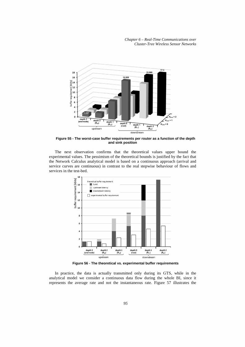
Chapter 6 – Real-Time Communications over Cluster-Tree Wireless Sensor Networks
95
Figure 55 - The worst-case buffer requirements per router as a function of the depth
and sink position
The next observation confirms that the theoretical values upper bound the experimental values. The pessimism of the theoretical bounds is justified by the fact that the Network Calculus analytical model is based on a continuous approach (arrival and service curves are continuous) in contrast to the real stepwise behaviour of flows and services in the test-bed.
Figure 56 - The theoretical vs. experimental buffer requirements
In practice, the data is actually transmitted only during its GTS, while in the analytical model we consider a continuous data flow during the whole BI, since it represents the average rate and not the instantaneous rate. Figure 57 illustrates the

Chapter 6 – Real-Time Communications over Cluster-Tree Wireless Sensor Networks
96
problem and shows the arrival and service curves of a data flow sent by an end-node to its parent router. The burst of the outgoing data flow �)�1�∗ is equal to ���KV , in case of the analytical model, or ���W-R , in the experimental case. Due to the cumulative flow effect, the differences between theoretical (���KV ) and experimental (���W-R ) values of buffer requirement grow with depth. The rate-latency service curve used in our analysis results from a trade-off between computing complexity and pessimism.
Figure 57 - Theoretical vs. experimental data traff ic
The numerical values of theoretical worst-case as well as experimental maximum buffer requirements are summarized in Table 5. In Table 5 and 6, U means an upstream router at depth i or an upstream link to a router at depth i, and D means a downstream router or a downstream link from a router at depth i.
Table 5 - Delay bounds: theoretical vs. experimenta l results
depth theoretical results
(worst-case values) experimental results (maximum values)
Ri [kbps] 'XY Qi [kbits] Qi [kbits]
Hsink = 0 (root)
0 U 1.7 3 15.995 5.376 1 U 0.39 1 7.329 2.304 2 U — — 2.008 0.768
Hsink = 1
0 D 1.56 4 8.667 3.072 U 1.17 3 — —
1 D — — 14.02 5.376 U 0.39 1 7.257 2.304
2 U — — 2.008 0.768
Hsink = 2
0 D 1.56 4 8.667 3.072 U 1.17 3 — —
1 D 2.34 6 15.966 4.608 U 0.39 1 7.257 2.304
2 D — — 17.3 5.376 U — — 2.008 0.768
end-node 0.39 1 1.337 1.344

Chapter 6 – Real-Time Communications over Cluster-Tree Wireless Sensor Networks
97
Delay Bounds In Figure 58, we compare the worst-case, maximum and average values of per-hop delays bound in each router, and the end-to-end delay bounds for Hsink = 2. A first observation confirms that theoretical values upper bound the experimental values. The difference in theoretical worst case (����KV ) and experimental maximum (����W-R ) delays is given by the aforementioned continuous and stepwise behaviors of the analytical model and test-bed, respectively. The experimental delays comprise mainly the service latencies (Figure 58) decreasing in the direction of the sink (Figure 51). Hence, the maximum per-hop delays also decrease in the direction of the sink as you can observe in Figure 58. The low downstream delay at depth 0 results from priority rule. The end-to-end delays bounds are quite high, even though the bdata and rdata are low. This is mainly due to high value of SO = 4 (i.e. BI = 1.966 sec). Hence, the end-to-end delay bounds can be reduced using lower values of SO or higher bandwidth guarantees, using lower IFS, for example.
Observe also that the worst-case end-to-end delay obtained by the per-flow approach offers less pessimism than the delay from the per-hop approach.
Table 6 presents the worst-case, maximum and average numerical values of per-hop and per-flow delay bounds, and the end-to-end delays for given sink position.
Figure 58 - Theoretical vs Experimental delay bound s
Note that the average values were computed from the set of 15 measurements, involving 1155 frames each.

Chapter 6 – Real-Time Communications over Cluster-Tree Wireless Sensor Networks
98
Table 6 – Delay bounds: theoretical vs. experimenta l results
depth theoretical results
(worst-case values) experimental results
maximum average Di [sec] Di [sec] Di [sec]
Hsink = 0 (root)
1 U 6.257 1.764 1.308 2 U 5.143 1.812 1.602
De2e 14.82/9.69 7.154 4.952
Hsink = 1
0 D 5.547 0.104 0.099 1 U 6.195 1.76 1.728 2 U 5.143 1.809 1.602
De2e 20.31/10.53 7.251 5.471
Hsink = 2
0 D 5.547 0.104 0.099
1 D 6.814 1.812 1.321 U 6.195 1.766 1.728
2 D 5.143 1.814 1.135 De2e 27.13/13.65 9.074 6.325
end-node (Ddata) 3.425 3.578 2.042
The determination of the optimal service curve, leading to the lowest worst-case delay, will be addressed in future work.
Lifetime of a WSN We have already mentioned previously that to maximize the lifetime of a WSN, low duty cycles are required. On the other hand, low duty cycles enlarge timing response of a WSN. Our assumptions are confirmed in Figure 59 which shows the theoretical worst-case and experimental maximum end-to-end delays as a function of duty cycle for Hsink = 0. The value of SO is set to 4 and the decreasing duty cycles are given by increasing BO. Note that the minimum BO is equal to 7 for SO = 4. To avoid the lack of bandwidth for lower duty cycles, the average arrival rate must be reduce to rdata = 0.190 kbps (�)�1�+,- = 0.195 kbps for duty cycle equal to 3.125%). The other network settings are the same as in previous experiments. The theoretical worst-case end-to-end delays are obtained by per-hop and per-flow approaches. The observation again confirms that the theoretical values upper bound the experimental values, and the worst-case delay obtained by the per-flow approach offers less pessimism than the delay from the per-hop approach.

Chapter 6 – Real-Time Communications over Cluster-Tree Wireless Sensor Networks
99
Figure 59 - The theoretical worst-case and experime ntal maximum end-to-end delays
as a function of duty cycle for Hsink = 0 (lifetime of a WSN)
6.6 Concluding remarks In this work, we tackled the worst-case dimensioning of cluster-tree wireless sensor networks (WSN) assuming that the data sink can be mobile, i.e. can be associated to any router in the sensor network. We developed a 7 clusters test-bed based on Commercial-Off-The-Shelf technologies, namely TelosB motes running our open-ZB protocol stack over TinyOS. This test-bed enabled us to assess the pessimism of our worst-case theoretical results (buffer requirements and message end-to-end delays), by comparing these to the maximum and average values measured in the experiments.
Importantly, we showed how it is possible to instantiate our generic methodology in IEEE 802.15.4/ZigBee, which are promising technologies for WSN applications.

Chapter 6 – Real-Time Communications over Cluster-Tree Wireless Sensor Networks
100

Chapter 7 ERIKA and Open-ZB: a Toolset for Real-Time
Wireless Networked Applications
IEEE 802.15.4/ZigBee and TinyOS have been playing an important role in leveraging a new generation of large-scale networked embedded systems. However, based on previous experience on the implementation and use of the IEEE 802.15.4/ZigBee protocols over TinyOS, several problems (producing loss of synchronization and even network crashes) emerge due to some limitations of TinyOS, namely related to the lack of task pre-emption and prioritization. Therefore, we implemented the IEEE 802.15.4 protocol over ERIKA, a real-time operating system for resource-constrained embedded systems. This chapter presents the most important aspects of the software implementation and reports comparative experimental results based on real hardware and software platforms.
7.1 Introduction IEEE 802.15.4 / ZigBee protocols provide timeliness guarantees when operating in beacon-enabled mode. This mode offers the possibility of allocating/ deallocating time slots in a Superframe, called Guaranteed Time Slots (GTSs), and therefore the possibility of providing predictable minimum service guarantees. Having a minimum service guarantee, it is possible to predict the worst-case timing performance of the network. Open-ZB [19] is an open source implementation of the IEEE 802.15.4 / ZigBee suite of protocols. It is however an implementation over TinyOS. The protocols are implemented through a number of carefully designed processing tasks. The design tries to minimize the impact of nonpreemption in delaying critical tasks such as the ones related to beacon transmission and generation. It is however proved [21] that when clusters operate at very high duty-cycles and beacon transmission frequencies, nodes may lose synchronization

Chapter 7 – ERIKA and Open-ZB: a Toolset for Real-Time Wireless Networked Applications
102
and therefore get disconnected from the rest of the network. Moreover, if a node is not properly synchronized, there is a possibility of collisions in the GTS slots (in case the CAP overlaps the CFP).
Non-preemption and lack of task prioritization is therefore the major drawback of the Open-ZB implementation of the ZigBee suite of protocols.
In order to overcome this problem, we propose, discuss and analyse an alternative implementation of the Open-ZB protocol stack over the ERIKA real-time OS [44]. The results hereby presented demonstrate that ERIKA enables reliable beacon synchronization, even under high duty cycles, and leads therefore to improved network performance when compared to implementations based on TinyOS. The main contribution of this work is the actual implementation of the IEEE 802.15.4 /ZigBee protocols over the ERIKA real-time operating system. It thus enables an open source tool suite that overcomes the problems of synchronization that occur in the implementation of the IEEE 802.15.4 over TinyOS.
7.2 Software Implementation
7.2.1 Architecture The implementation of the IEEE 802.15.4 protocols over ERIKA is organized in a layered architecture. In this design we build the networking stack by the use of Operating System primitives, generic libraries and the hardware features provided by the Micro-Controller Unit (MCU). Figure 60 illustrates the overall software architecture.
Figure 60 – Stack implementation layered architectu re
The HW layer abstracts the current selection of hardware components including the Microchip dsPic33F MCU, CC2420 Chipcon transceiver, and the FLEX development board (embedding LCD, LEDS, etc., see Chapter 3 concerning technologies). To ensure a clean design, the hardware-driven facilities are separated from the rest of the implementation. In the HW interrupts layer the ERIKA Interrupt Service Routines (ISRs) are implemented to handle all hardware interrupts. Moreover, in the ieee802 15 4 layer all the hardware related attributes specific for implementing the IEEE 802.15.4 communication protocol were implemented separately. This layer contains the code to initialize the hardware timers, to initialize the communication between CC2420 transceiver and MCU, and to handle timer and transceiver interrupts. The CC2420 driver

Chapter 7 – ERIKA and Open-ZB: a Toolset for Real-Time Wireless Networked Applications
103
is a component for sending commands to and exchanging data I/O with the transceiver. This driver exports to Transceiver-HAL all the primitives standardized in IEEE 802.15.4 PHY. The Transceiver-HAL is a helper layer aware of the upper IEEE 802.15.4 MAC and CC2420 driver, designed to extend the support to different hardware solutions. The ERIKA layer is responsible for managing the system hardware resources and is providing the typical OS services such as Task management, resource access control, interrupt and timer management. Software timer abstractions are provided by means of software counters and alarms.
Alarms are software abstractions for timers. These alarms are used in this context to activate periodic tasks. ERIKA alarms, configured for communication purposes, can be initialized with a desired rate, stopped and reset whenever required. The common lib is a generic library providing some software utilities to the upper layers. More specifically, this layer provides: basic data structures such as queues, circular queues, indexed structures, etc used in memory buffer management; debugging helper, e.g. utilities for printing data on the console using the serial communication with the MCU through the UART port. The ieee802 15 4 Lib is the heart of the network stack. It includes the PHY and MAC layers of IEEE 802.15.4 standard. This layer is concerned only with the implementation details of the communication, and makes use of the timing services and memory management services provided by underlying layers. The IEEE 802.15.4 physical layer (shown in Figure 61) is responsible for the implementation of the following functionalities:
− Activation and deactivation of the radio transceiver; − Channel frequency selection; − Energy Detection(ED) within the current channel; − Turnaround of the radio; − Link quality indicator (LQI) for received packets; − Clear Channel Assessment (CCA) for Carrier Sense − Multiple Access Collision Avoidance (CSMA-CA).
Figure 61 - PHY Layer reference model
The Physical Data Service Access Point (PD-SAP) is responsible for receiving and sending the data from and to the MAC layer. The Physical Layer Management Entity SAP (PLME-SAP) includes the interfaces between the MAC and the PHY used for exchanging management information.

Chapter 7 – ERIKA and Open-ZB: a Toolset for Real-Time Wireless Networked Applications
104
Figure 62 - MAC layer reference model
The IEEE 802.15.4 MAC layer (shown in Figure 62) is responsible for the implementation of the following functionalities:
− Generating network beacons if the device is a coordinator; − Synchronizing to the beacons; − Supporting PAN association and disassociation; − Supporting device security; − Employing the CSMA-CA mechanism for channel access; − Handling and maintaining the GTS mechanism; − Providing a reliable link between two peer MAC entities.
7.2.2 Implemented services Currently we have implemented most of the basic mechanisms of Open-ZB over ERIKA. We developed a fully functional, customized driver for the CC2420 transceiver. Our libraries support the generation of the MAC superframe and provide the slotted CSMA/CA access mechanisms. The protocol services have been mapped to tasks having reserved a set of priorities for network-related use only. Regarding memory usage, buffer queues have been statically allocated in the global scope to accommodate message payloads (MPDU) used for send and receive. Concerning networking we enabled the modules related to MAC & PHY services in the Open-ZB package. More precisely we implemented Beacon transmission at every Beacon Order, Static Network formation (i.e. without negotiation and with statically assigned MAC addresses), Coordinator/ End device time synchronization using CSMA/CA slotted mode. Thus, we enable data transmission and reception in unslotted and slotted mode including GTS allocation and transmission. Since negotiation is not yet implemented, currently it is up to the application programmer to actually define network addresses and to allocate GTS slots for end devices.
7.2.3 Implementation details To configure the network stack in ERIKA we use the OIL language: this includes the creation of the tasks required by IEEE 802.15.4 protocol, their respective priorities, the usage of ERIKA alarms and the choice of a scheduling policy. In Table 2 we list the service tasks assigned together with their priorities, the periods and the associate alarms used for their activation.

Chapter 7 – ERIKA and Open-ZB: a Toolset for Real-Time Wireless Networked Applications
105
Most of these tasks are periodic with rate dependent on the IEEE 802.15.4 protocol specification, Beacon Order (BO) and Superframe Order (SO) settings. To generate these precise timing values we make use of a 16 bit hardware timer provided by dsPic33F processor. This timer has a minimum tick value of 0.025 µs when the microcontroller is configured to work at 40 MHz operating frequency.
The hardware timer is set to have a granularity of 320 µs required by the backoff interval specified in the IEEE802.15.4 standard. All the networking tasks depend on it since their activation periods are integer multiples of 320 µs. Concerning memory, in our design we make use of three memory buffers. These global memory locations are shared by different modules and require mechanisms for mutual exclusion and synchronization: ERIKA “resources” have been used for such a purpose (see Table 7).
Table 7 - Memory buffers and ERIKA resources set as guards
In the IEEE 802.15.4 framework, beacon transmissions are used to synchronize the devices. Thus, in our implementation the alarms are re-aligned after the beacon has been recognized and processed.
The algorithm works as follows (see Figure 63). At the firing of an event of Start of Frame Delimiter SFD) from the radio, an ISR interrupt handler is executed. In the handler code, a clock timer is activated tracking the time needed to recognize the packet as a beacon. Next, at the firing of the FIFOP event (denoting that the RX buffer has been filled), the ReadDispatcher (high priority) task is activated. After reading the first 3 bytes of the packet (enough to know the packet type), if the packet is recognized as a beacon, the task continues its execution (safe from eventual pre-emption) until all information carried by the beacon are processed and the timer is stopped (the counter reads ∆T ); if the packet is not a beacon another task is in turn activated to process the data at a lower priority. The information on ∆T are used to synchronize the alarms with the arrival of the beacon (SFD), having taken note of the beacon reception and processing overhead. In our experiments, ∆T has never exceeded 1.9 ms. This number is probably dominated by the transceiver response time (i.e. the time needed to receive all bits of the beacon, and transmit them over the SPI bus).
Figure 63 - Beacon processing in ERIKA

Chapter 7 – ERIKA and Open-ZB: a Toolset for Real-Time Wireless Networked Applications
106
7.3 Experimental work
7.3.1 Data collection and analysis method The implementation of the IEEE 802.15.4/ZigBee has been validated by using the Chipcon CC2420 Packet Sniffer. The CC2420 Packet Sniffer for IEEE 802.15.4 v1.0 provides a raw list of the packets transmitted. Thanks to this hardware/software suite, it is possible to collect detailed record of the packets transmitted over air by all WSN devices and analyze them off-line.
7.3.2 Beacon Transmission Timing Coherence and Clock Drift calculation As already mentioned in Section 3.1, to transmit the beacons, we use ERIKA alarms. In order to measure the time coherence in beacon transmission we used the timestamping support of the Chipcon testing suite. At Beacon Order (BO) of 6 we obtained the results as shown in Figure 64.
Figure 64 - Beacon inter-arrival time at the sniffe r board
Analyzing the plot, and neglecting any spread in propagation time (of the order of a few ns), we observe that ERIKA is about 50 µs late with respect to the nominal value. This effect is proven in the following to be due to the clock drift accumulated at the source device in one BI. Although displaced, the ERIKA alarm coherence is in the order of 1 µs. We measured the Beacon Interval letting the BO vary from 0 to 8. The results are shown in Table 11.

Chapter 7 – ERIKA and Open-ZB: a Toolset for Real-Time Wireless Networked Applications
107
Table 8 - Observed time divergence from nominal val ue
The observed trend as function of BO demonstrates that the effect is due to the clock drift. From the value corresponding to BO = 8, we can even estimate the clock drift as:
This is true, assuming equal accuracy for the dsPic33F and the Chipcon Sniffer Board.
7.3.3 Contention Free Transmissions We prepared an experimental setup consisting of 3 nodes: one PAN coordinator and 2 transmitting node devices.
Following the IEEE 802.15.4 standard, GTS allocation is performed by the PAN coordinator, which in our setup allocates two GTSs (4 time slots wide each) to the other nodes, as shown in Figure 65. Multiple frame transmission has been implemented in device nodes spanning the total duration of the allocated bandwidth. Following the standard, a set of 12 frames are injected into the network without contention by each device at every superframe. In a set of runs, each composed by about 400 beacons at BO = 4, the CC2420 packet sniffer detected on average 99% of the scheduled transmissions. The few missed frames are due to frame error occurrences probably caused by interference with IEEE 802.11 channels.
7.4 Comparative performance results In this section, we compare the performance (throughput and packet delivery ratio) of our hardware/software platform (ERIKA + Open-ZB) with respect to other popular ones, namely:
− TinyOS 2.0 and BMAC on Telos-B; − TinyOS 2.0 and Open-ZB on Telos-B.

Chapter 7 – ERIKA and Open-ZB: a Toolset for Real-Time Wireless Networked Applications
108
Figure 65 - Guaranteed Time Slots allocated to Devi ce 1 and 2 to inject packets
without contention access
Our testbed consists of a multi-task firmware with the Constant Bandwidth Rate (CBR) traffic generator scheduled together with the other tasks implementing the network stack services. The payload (104 bytes), and the number of transmitted packets (1000) are fixed. The inter-frame period (i.e. the inverse of the traffic rate) is a tunable parameter. The number of delivered packets and the total elapsed time are extracted from the Chipcon sniffer application.
7.4.1 Downsizing FLEX to Telos-B Unfortunately, an implementation of ERIKA for the Telos-B board is not yet available. The dsPic processor on the FLEX board normally runs at 40 MHz, whereas the Texas Instrument MSP430 processor used on the Telos-B has a maximum processor frequency of 8 MHz. To remove the bias in comparing these two platforms, we prescaled the dsPic internal clock by a factor of 5, thus operating it at 8MHz. In addition, we set the SPI frequency for MCU – radio I/O in both platforms to the same frequency of 1 MHz. Finally, in both implementations, we allocated memory buffers of the same size for packets.
Thus, apart from the instruction set architectures, the two platforms are equivalent. For better comparison, we run the same experiments on the FLEX both at full speed and at the pre-scaled frequency. As shown in Figure 66, the effect introduced by the CPU speed is not negligible at low rate, up to about 200 Hz. However, above this threshold the role played by the hardware is very limited with respect to software effectiveness, as it will be shown in the next section.
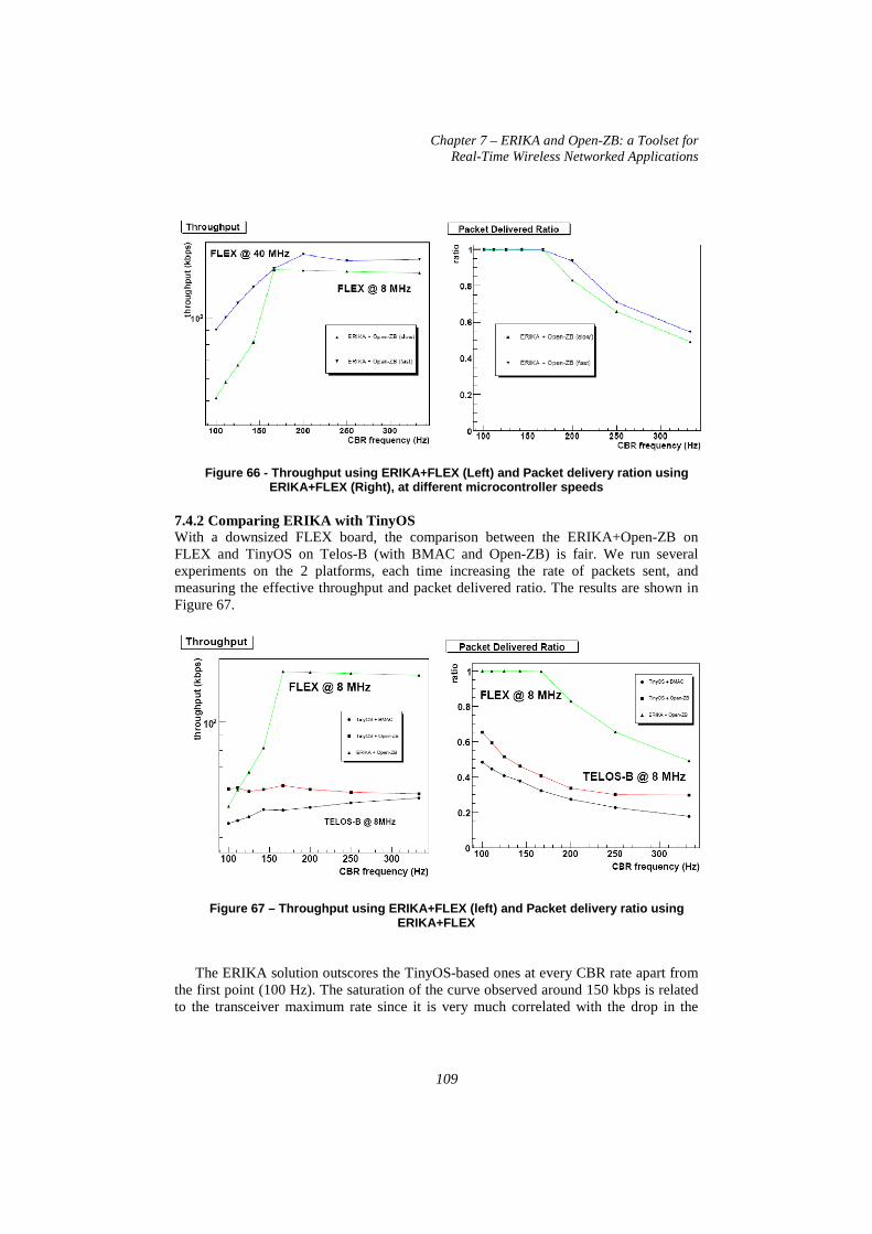
Chapter 7 – ERIKA and Open-ZB: a Toolset for Real-Time Wireless Networked Applications
109
Figure 66 - Throughput using ERIKA+FLEX (Left) and Packet delivery ration using ERIKA+FLEX (Right), at different microcontroller sp eeds
7.4.2 Comparing ERIKA with TinyOS With a downsized FLEX board, the comparison between the ERIKA+Open-ZB on FLEX and TinyOS on Telos-B (with BMAC and Open-ZB) is fair. We run several experiments on the 2 platforms, each time increasing the rate of packets sent, and measuring the effective throughput and packet delivered ratio. The results are shown in Figure 67.
Figure 67 – Throughput using ERIKA+FLEX (left) and Packet delivery ratio using ERIKA+FLEX
The ERIKA solution outscores the TinyOS-based ones at every CBR rate apart from
the first point (100 Hz). The saturation of the curve observed around 150 kbps is related to the transceiver maximum rate since it is very much correlated with the drop in the

Chapter 7 – ERIKA and Open-ZB: a Toolset for Real-Time Wireless Networked Applications
110
delivered ratio (i.e. probability of successful transmission). Moreover we found the ERIKA + Open-ZB solution more convenient up to about 400 Hz.
7.5 Concluding remarks The rising demand for using WSNs in industrial automation and new exciting application domains as distributed video processing require support for hardware/software platforms exhibiting real-time behaviour. However, popular and widespread operating systems like TinyOS cannot support real-time behaviour in this context. To overcome these limitations, we decided to implement a software suite integrating the ERIKA OS real-time kernel with the Open-ZB network stack. In this chapter we presented the architecture of our software and the internal implementation.
Although the work is not yet complete, most of the services are operational and a complete set of tests have been presented in this chapter to validate our implementation. The results are very encouraging. Our hardware/software platform can achieve very high throughput and packet delivery ratio with respect to existing solutions based on TinyOS. Moreover, we show a high timing coherence in the beacon transmission and high reliability in packet delivery.
Given these concrete and promising results, we firmly believe that it is indeed possible to provide support for real-time execution and network transmission in cheap hardware platforms. Currently, we are completing the implementation of all the services in Open-ZB, including bandwidth allocation strategies and support for application-level QoS management and control. In the near future, we plan to use our platform to carry on advanced research on distributed video processing in dense WSNs. It is also envisaged to implement the core ZigBee Network Layer functionalities to support multi-hop communications, namely Cluster-Tree network topologies.

Chapter 8 Hands-on Work over a Real Application
Scenario
This chapter presents a deployment of a Wireless Sensor Network in a real application scenario. This scenario aims at demonstrating the impact of the presence of hidden-nodes in a real target tracking application. Some of the problems and challenges faced are discussed, namely in what concerns technological limitations, as well as some hands-on experience gained from this implementation.
8.1 Introduction Target tracking applications are highly demanding in timeliness and therefore very appealing to serve as platforms for testing and demonstrating the real-time operation of a network. This premise lead to the development of a Search and Rescue application ([87], [88]) for testing, validating and demonstrating the architecture and mechanisms of the ART-WiSe research framework [11]. A first approach to this application was reported in [12].
In this chapter we propose to assess and demonstrate the impact of the hidden-terminal problem in a real WSN application. With this purpose a new application scenario was built over the aforementioned Search and Rescue testbed application.
During the development of the application some challenges were faced. Most of them were related to technological limitations in terms of hardware, timer handling and operating system limitations. These problems are reported here, as well as some physical layer aspects such as coexistence problems between IEEE 802.15.4 and IEEE 802.11 radio channels.

Chapter 8 – Hands-on Work over a Real Application Scenario
112
8.2 Snapshot of the ART-WiSe Search & Rescue testbed application The overall objective of the application is to detect, localize and rescue a target entity, within a certain region covered by a WSN deployment. Mobile robots are currently being used to act as target and rescuer/pursuer entities [87].
The target robot is supposed to be in distress (search&rescue context) or to be an intruder (pursuit-evasion context). The target robot movement is remotely controlled by an operator, using a joystick. A WSN node mounted on top sends periodic messages to signal its presence, which are then relayed by the WSN to the Control Station with the necessary data to trigger localization. The Control Station then computes the target robot location, displays it in a virtual scenario and informs the rescuer robot that will immediately initiate its mission by moving towards the last known position of the target robot. This process is repeated until the rescuer robot is close enough to the target robot. Figure 68 illustrates an example scenario.
Figure 68 - Snapshot of the ART-WiSe Search&Rescue Testbed Application
On the top right corner of Figure 68 it is showed the Control Station software Graphical User Interface (GUI). In that software it is presented a virtual representation of the testbed scenario as well as a video stream from the Rescuer camera and other information regarding the Rescuer status.

Chapter 8 – Hands-on Work over a Real Application Scenario
113
Figure 69 - The Search&Rescue Testbed in action
Figure 69 shows a picture from the ART-WiSe Search and Rescue testbed in action.
8.3 Overview of the testbed localization mechanism The developed localization mechanism is based in RSS (Radio Signal Strength) readings from the CC2420 transceiver [28] used by the WSN nodes (MICAz). The target robot detection mechanism and the subsequent mission dispatching to the rescuer robot are illustrated in Figure 70 in the timing diagram of Figure 71.
Figure 70 - The localization mechanism
The target robot initiates the process by announcing its presence by sending a distress (“help”) broadcast message (2a) at a pre-programmed transmission power and timing rate. Every WSN node that receives that distress message stores the received RSSI and builds a “Distress Alert message” containing that value and its coordinates and sends it to the control station (2b). The Control Station is expected to receive multiple “Distress Alert messages” from different nodes. As soon as a sufficient number of messages is received (e.g. 7 messages) the target robot’s position is computed based on the same algorithm used for the rescuer robot positioning.
Message WSN node Triggered Node
Control Station
Rescuer robot
Target robot
2a
2b
2b
2b
1a
2c
1a
1a
1a

Chapter 8 – Hands-on Work over a Real Application Scenario
114
Broadcast Message
Calculate Target Position
Virtual Display
Process New Mission / Mission
Update
Multiple detection messages
Status message
Status message
New Mission / Mission Update
Rescuer Robot
Control Station
WSN NodesTarget Robot
IEEE 802.15.4
IEEE 802.15.4
IEEE 802.11
IEEE 802.11
IEEE 802.11
(2a)
(2b)
(2c)
Figure 71 - Timing diagram of the localization mech anism
The localization mechanism presented a maximum error of approximately 70 cm. We
did not expect better results for the localization mechanism since there are many sources of RSSI variability like transmitter/receiver variability, antenna orientation and multi-path fading and shadowing. All these reasons may cause errors in the RSSI measurements, eventually leading to the computation of a wrong position. The localization mechanism is presented in more detail in [87].
8.4 Assessing the hidden-node impact in the application
8.4.1 Changes to the testbed In order to assess the impact of the presence of hidden-nodes in the behaviour of the testbed, a hidden-node zone (HNZ) was created inside the WSN deployment. Within this area, some nodes were programmed as hidden-terminals, by changing the CCA (Clear Channel Assessment) Threshold value of the node’s transceiver to a maximum value, so that they would not be able to sense the wireless channel as busy.
The Rescuer robot was not used in the experiments since we focused more on assessing the hidden-terminal impact in the tracking capabilities of the application, rather than in performing communication to a higher tier (IEEE 802.11 for communicating with the Rescuer robot).
8.4.2 Impact in the localization mechanism In order to measure the impact in the application, namely in the localization and target tracking mechanism, we carried out two different sets of experiments. Those were to measure the necessary time to get a precise localization of the Target Robot when inside the HNZ as compared to the normal behaviour (without hidden-nodes).

Chapter 8 – Hands-on Work over a Real Application Scenario
115
In the first one, we set the WSN nodes that were triggered in the localization mechanism (the anchor nodes) as hidden and measured the delay to get a localization output. On the second set of experiments we used only one hidden node placed inside the HNZ generating traffic at preset rates. This node could not sense the four anchor nodes necessary for localization. However, this time the anchor nodes were able to sense each other and the extra traffic generating node, thus resulting in a unidirectional link between those and the hidden-node. Ten measurements were performed for each traffic value.
In both tests, one set of experiments was done using the H-NAMe [14] mechanism, described in Chapter 5, to demonstrate the feasibility and effectiveness of the mechanism in a real application scenario. Test 1 For Test 1, we used only one hidden anchor node, then two, three and finally all the four anchor nodes as hidden-nodes, leaving in the last case, no link between them. Figure 72 presents the time necessary to get the localization of the target for each case.
Figure 72 - Delay in Localization for Test 1
With all the four anchor nodes programmed as hidden nodes, the delay to get a correct location output was higher than 30 seconds. On the other hand, without any hidden-node the time necessary to get the position of the target is less than 1 second (approximately 400ms).
We noticed that with only one hidden-node of the four anchor nodes in the HNZ, there was little impact on the delay. This was due to the fact there were always three anchor nodes with full connectivity and distance information available (the minimum to run the localization algorithm). In fact, when we disconnected one of those three anchor nodes, the delay value increased to 5 seconds, since there were only two nodes with full connectivity available for performing localization.
With the H-NAMe mechanism, we assigned one group to each hidden-node. The performance improvement was immediately noticed, since it allowed localization in approximately one second, even when all of the four anchors used for localization were hidden.
Could not get a position result

Chapter 8 – Hands-on Work over a Real Application Scenario
116
Test 2 A hidden-node was programmed to generate traffic with pre-programmed inter-arrival times. It was then placed inside the HNZ. The target was also placed inside the HNZ and the localization mechanism was enabled. Several sets of experiments were made for different traffic generation rates (ten for each inter-arrival time). This test is different from the previous in the sense that now there is a unidirectional link between the anchor nodes and the hidden-node (the anchor nodes can sense the hidden-node but the hidden-node cannot sense the anchors). Interference was not expected to be very high since the anchor nodes could use the IEEE 802.15.4 Slotted CSMA-CA for performing collision avoidance, thus escaping collisions with the hidden-node. Nevertheless, some delay was still observed as showed in Figure 73.
Figure 73 - Delay in localization for test 2
For low inter-arrival times (around 1 second), there is little impact on the delay since the probability of collisions is not very high. Nevertheless, for an inter-arrival rate of one second, there were still collisions, leading to a delay around four seconds. However, as the inter-arrival time tends to decrease (lower than 100 ms), the impact is highly noticeable, taking approximately 20 seconds to get the position of the target. This obviously renders the localization mechanism useless and the tracking application fails, since it takes too much time to output a target position. On the other hand, when H-NAMe is used, the delay remains approximately the same (around 1 second), as it is completely independent from the hidden-node traffic rate.
This test was repeated with the target robot in motion (remote controlled) at a constant speed. As expected, we observed that for inter-arrival values lower than 800 milliseconds in the traffic generating node, as the robot was going through the HNZ, the Control Station failed to present its current position. As the robot left that zone, the Control Station was able to correctly inform the position of the target once again. When using H-NAMe, the localization output from the localization mechanism was constant, both inside and outside the HNZ zone.

Chapter 8 – Hands-on Work over a Real Application Scenario
117
8.5 Problems and challenges related to the experimental work When dealing with actual implementation work, one is probable to face challenges related to the technological limitations of the platforms under use. This is particularly true when using recent technology like the one available for WSNs.
In the course of our research work, several experimental scenarios were built for testing and validating our theoretical proposals. Some examples include the network performance evaluation testbeds described in Chapter 4 and 5 and the one used for the worst-case dimensioning of Cluster-Tree ZigBee networks presented in Chapter 6. All of these presented some challenges that had to be mitigated to enable the envisaged experimental validation.
During this particular implementation and experimental efforts, some of those difficulties were re-encountered, namely in what concerns the behaviour of the hardware platforms – the MICAz and TelosB motes. In this section, we summarize some relevant problems we faced during this implementation effort and others, already described in previous chapters, and how they have been tackled.
8.5.1 Hardware platforms and debugging The MICAz mote requires the use of a hardware board as a programming interface (the MIB510), while the TelosB mote features an USB interface, enabling the programming via the PC. Both motes provide a debug mechanism by sending data through the serial (COM/USB) port and reading it in a communication listener (e.g. ListenRaw, provided with the TinyOS distribution, or Windows HyperTerminal). This debugging mechanism raises a problem concerning the hardware operation, since the transmission through the COM port blocks all the other mote operations. This usually causes synchronization problems.
In order to overcome these local debugging issues and to have a total control over the network behaviour and of all transmitted packets, we have been using two different network/protocol analysers [37] and [38] already described in detail in Chapter 3.
8.5.2 Memory constraints The mote platforms we have used in the IEEE802.15.4/ZigBee implementation – MICAz and TelosbB – are very limited in terms of random access memory (RAM) – roughly 4 kB for the former and 10 kB for the latter. The RAM must be sufficient to fulfil the requirements of the TinyOS operating system, of the protocol stack and of the high level application. In this aspect, the MICAz motes are more constrained than the TelosB. Take the example of two TinyOS 2.0 demo applications in order to demonstrate the variation in RAM memory usage – the Blink and MultihopOscilloscopeApp applications, compiled for both platforms. The first uses approximately 55 bytes and the second 3348 bytes of RAM. Besides the RAM memory allocated at compilation time, the devices need to have enough free memory for the operating system stack. In our TinyOS 2.0 implementation, the memory needed by an application that only uses the IEEE 802.15.4 beacon-enabled modes needs approximately 2678 bytes of RAM while an application using the ZigBee network layer with the cluster-tree topology needs approximately 3224 bytes. Note that it is assumed that the high level applications are

Chapter 8 – Hands-on Work over a Real Application Scenario
118
very simple and just used for testing purposes and the different buffers used are very small.
8.5.3 CC2420 transceiver limitations Another hardware limitation concerns the radio performance of the CC2420 transceiver, used by the MICAz and TelosB motes. According to the IEEE 802.15.4 Physical Layer specification, the transceiver must have a turnaround time, i.e. the time that the CC2420 radio transceiver takes to switch from receive mode to transmit mode and vice-versa, of 12 symbols (192 µs). This is the maximum time bound required to acknowledge messages. In fact, the CC2420 has the hardware configuration of auto-acknowledge messages but, besides generating several false acknowledgments (messages that are acknowledge but not received by the protocol stack) it needs to have the address decode functionalities activated. Unfortunately, similarly to several IEEE 802.15.4 compliant transceivers, it is not possible to achieve the specified turnaround time.
For instance, the Chipcon CC2420 can take up to 192 µs just to switch between these two modes, leaving no time for data transitions between the MAC sub-layer, the PHY layer and the chip transmit memory space.
In addition, the processing power available in the motes microcontroller revealed to be quite limited to comply with the most demanding IEEE 802.14.5 timing constrains, especially for small Beacon orders (BO < 3) and Superframe orders (SO < 3). This turns these Superframe configurations impossible to deploy, considering that the motes must also have availability for processing other tasks. It is reasonable to assume that the processing limitations can be easily overcome in the near future with the development of new and faster microcontrollers or by a hardware implementation of the protocol stack.
8.5.4 Timing and synchronization requirements The timing requirements of the IEEE 802.15.4 protocol are very demanding. In the beacon-enabled mode, all devices (ZRs and ZEDs) must synchronize with their parents (ZR or ZC) through beacon frame signalling. If a device loses synchronization it cannot operate in the PAN. Moreover, if a node is not properly synchronized, there is a possibility of collisions in the GTS slots (when the CAP overlaps the CFP). As experienced in our implementation, the loss of synchronization can be caused by multiple factors, such as: (1) the processing time of the beacon frame for low BO/SO configurations; (2) the mote stack overflow that results in a processing block or a hard reset; (3) the unpredictable delay of the wireless communications; and (4) the reduced processing capability of the microcontroller in conducting some of the protocol maintenance tasks (e.g. creating the beacon frame, the maintenance of GTS expiration and indirect transmissions).
The implementation of the slotted CSMA/CA algorithms is also quite demanding in terms of timer accuracy, since the IEEE 802.15.4 protocol defines that each backoff period corresponds to 20 symbols (320 µs). A first difficulty in the implementation of the beacon-enabled mode was related to the TinyOS management of the hardware timers provided by the motes, which do not allow having the exact theoretical values of the BI, SD, time slot and backoff period durations as specified by the IEEE 802.15.4 standard. This discrepancy, however, does not impact the correct behaviour of the implemented protocol; provided that the same mote platforms are used in the experiments (at least as ZC and ZRs), it is possible to experience a coherent network behaviour.

Chapter 8 – Hands-on Work over a Real Application Scenario
119
Figure 74 - Asynchronous events
The frequency of the asynchronous software events (Figure 74), the hardware events and the low microprocessor processing ability may lead to an insufficient processing time left to execute remaining protocol and higher level application tasks, as a great amount of interrupts have to be processed in short periods of time.
8.5.5 TinyOS task scheduler This was already discussed in greater detail in Chapter 7. The default scheduler of TinyOS does not support tasks prioritization and, furthermore, the TinyOS scheduler is non pre-emptive. Although, with the aforementioned problem, the protocol stack behaves steadily for beacon and superframe orders higher than 3, this constitutes a problem for other BO/SO settings.
8.5.6 Interference between radio channels To ensure the reliability of the measurement process, some issues had to be considered, namely guaranteeing that the IEEE 802.15.4 physical channel was free from interference from IEEE 802.11 networks, which operate at the same frequency range. We have experimentally observed that despite the distance to the nearest IEEE 802.11 access point being over 10 m, it definitely impact on the performance measurements. The channel was often sensed as busy (during the Clear Channel Assessment (CCA) procedure) due to IEEE 802.11 transmissions. Hence, we chose an IEEE 802.15.4 channel outside the IEEE 802.11 frequency spectrum (Channel 26) to perform the experimental evaluation. Channel integrity was ensured using a spectrum analyzer. In addition, another aspect that was considered was the choice of the SO value to be used in our experiments.
In order to experimentally analyse the behaviour of the protocols, we devised scenarios that enabled us to evaluate different network metrics, such as the Network Throughput and Probability of Success as a function of the network load, as reported in Chapter 4, 5 and 6. Other scenarios, like the one described in this chapter, had the goal of demonstrating impact of some parameter in a real application. In general lines, these scenarios consisted of one or several nodes programmed to generate packets at the application layer with preset inter-arrival times, enabling us to push the necessary traffic load into the network. We used the previously referred IEEE 802.15.4 protocol analyzer to log the received packets and developed an application to parse the message payload, which embedded relevant performance information retrieved from the nodes in order to compute the required metrics.

Chapter 8 – Hands-on Work over a Real Application Scenario
Obviously, it is important to isolate as much as possible the testbed scenario from external factor that may impact in the
One requirement of the performance evaluation was to achieve high traffic loads in the network, namely pushing well above 100observed that it was not only difficult to get a consistent behaviour of the Throughput metric but also to get high offered loads. Moreover, it was hard to ensure the stability of the network when the nodes were ge
After performing several assessments, we reached the conclusion that this behaviour was mostly related to three factors: (1) the interference from the Withe laboratory (see Figure the node’s scarce processing capability.
The interference between IEEE 802.11 and 802.15.4 radio channels, ca spectrum analyser, had unpredictable effects on the results. We observed that the interference of IEEE 802.11 networks often generated collisions with data/beacon frames. This effect, lead to data corruption and network dealso had implications on the amount of traffic sent to the network because in the IEEE 802.15.4 slotted CSMA/CA protocol, the medium was often sensed as busy (during the Clear Channel Assessment (CCA)), causing deference and failed transmissiobviously affected the behaviour of the network since it did not allow reaching the desired traffic loads. We overcame the interference problem by using the only IEEE 802.15.4 channel (Channel 26 in the 2480 MHz frequency band) that is completelyoutside the IEEE 802.11 frequency spectrum
Figure
Note that this interference must be taken into consideration for the reliable deployment of ZigBee networks operating in the 2.4 GHz frequency. Nevertheless, besides the interference problem, we have also identified other sources of inconsistencies.
on Work over a Real Application Scenario
120
Obviously, it is important to isolate as much as possible the testbed scenario from external factor that may impact in the
One requirement of the performance evaluation was to achieve high traffic loads in the network, namely pushing well above 100% of the network capacity. We immediately observed that it was not only difficult to get a consistent behaviour of the Throughput metric but also to get high offered loads. Moreover, it was hard to ensure the stability of the network when the nodes were generating packets with very low inter-arrival times.
After performing several assessments, we reached the conclusion that this behaviour was mostly related to three factors: (1) the interference from the Wi-Fi networks around
Figure 76); (2) TinyOS-related constrains; and (3) others related to the node’s scarce processing capability.
The interference between IEEE 802.11 and 802.15.4 radio channels, confirmed using a spectrum analyser, had unpredictable effects on the results. We observed that the interference of IEEE 802.11 networks often generated collisions with data/beacon frames. This effect, lead to data corruption and network de-synchronization. Moreover, it also had implications on the amount of traffic sent to the network because in the IEEE 802.15.4 slotted CSMA/CA protocol, the medium was often sensed as busy (during the Clear Channel Assessment (CCA)), causing deference and failed transmissiobviously affected the behaviour of the network since it did not allow reaching the desired traffic loads. We overcame the interference problem by using the only IEEE 802.15.4 channel (Channel 26 in the 2480 MHz frequency band) that is completelyoutside the IEEE 802.11 frequency spectrum as depicted in Figure 75.
Figure 75 - IEEE802.15.4 and IEEE 802.11 channels
interference must be taken into consideration for the reliable deployment of ZigBee networks operating in the 2.4 GHz frequency. Nevertheless, besides the interference problem, we have also identified other sources of
Obviously, it is important to isolate as much as possible the testbed scenario from
One requirement of the performance evaluation was to achieve high traffic loads in % of the network capacity. We immediately
observed that it was not only difficult to get a consistent behaviour of the Throughput metric but also to get high offered loads. Moreover, it was hard to ensure the stability of
arrival times. After performing several assessments, we reached the conclusion that this behaviour
Fi networks around related constrains; and (3) others related to
onfirmed using a spectrum analyser, had unpredictable effects on the results. We observed that the interference of IEEE 802.11 networks often generated collisions with data/beacon
Moreover, it also had implications on the amount of traffic sent to the network because in the IEEE 802.15.4 slotted CSMA/CA protocol, the medium was often sensed as busy (during the Clear Channel Assessment (CCA)), causing deference and failed transmissions. This obviously affected the behaviour of the network since it did not allow reaching the desired traffic loads. We overcame the interference problem by using the only IEEE 802.15.4 channel (Channel 26 in the 2480 MHz frequency band) that is completely
interference must be taken into consideration for the reliable deployment of ZigBee networks operating in the 2.4 GHz frequency. Nevertheless, besides the interference problem, we have also identified other sources of

Chapter 8 – Hands-on Work over a Real Application Scenario
121
Figure 76 - WiFi networks around the Hands-on lab
As already discussed in Section 3, TinyOS imposes several limitation that influence the behaviour of the protocol stack, namely on the synchronization. We have observed that when nodes used a very low inter-arrival time (in the order of 50 packets per second) the de-synchronization was a concern, mainly due to the high amount of tasks posted to generate the required offered load. To mitigate this problem, we programmed the nodes to generate packets only during the active portion of the Superframe, trying to guarantee that the beacon frame would be parsed immediately upon the reception. Nevertheless, when using a full duty cycle the problem remained. We have solved it by using a new timer that fires a few milliseconds before the end of the Superframe, stopping all the packet generation and leaving the nodes ready to process the beacon.
8.5.7 RSSI-based localization inaccuracy In the Search&Rescue application described in this chapter, a rescuer robot is supposed to track and reach, in the minimum amount of time, a steady or moving target (person or robot), using a wireless sensor network for tracking and localization. In this context we wanted to develop a simple but effective localization mechanism, relying as much as possible on COTS technologies and taking advantage of the RSSI indicator available directly from the CC2420 transceiver, using the RSSI values as the source for distance estimation.
We immediately observed that these measurements were highly sensitive to ambient conditions. The proximity to metal and walls highly increased the number of reflections leading to non-consistent RSSI readings. Moreover, the RSSI value was not linear with the distance (Figure 77) and it varied with different mote antenna orientations. This means that it was probable to find several different RSSI readings at the same distance. To overcome that problem, several experiments were carried out at different distances, transmission powers and antenna orientations in an attempt to get a consistent set of values for different distances ([87], [88]).
After these experiments, it became possible to establish a correspondence between discrete range levels and the spread of RSSI values encountered for that same range.

Chapter 8 – Hands-on Work over a Real Application Scenario
122
Figure 77 - RSSI versus Distance [88]
This enabled us to engineer a simple RSSI-based localization mechanism with approximately 60 cm inaccuracy, which was acceptable for the envisaged application.
8.6 Concluding Remarks In this chapter we presented a deployment of a WSN in a real scenario (a target tracking application), aiming at demonstrating the impact of the hidden-node problem and to prove the effectiveness of the H-NAMe mechanism.
We showed that this issue greatly affects an application of this kind, by increasing the message delays (through multiple collisions), thus reducing the effectiveness of the localization mechanism in the proximity of hidden-nodes. In fact, from our tests, we showed that having two out of four anchor nodes (used in the localization mechanism) hidden, is enough to cause a significant degradation of the target localization process, taking up to five seconds to get a result.
We also evaluated the impact of having only one hidden-node placed inside the network generating traffic at different rates. We proved that one node, with a medium traffic generation rate (800 milliseconds), would cause problems to the localization process.
We also reported several problems and challenges emerging from our experimental work on the IEEE 802.15.4/ZigBee protocol stack. The hardware platforms under use – MICAz and TelosB – seem to be too limited for the demanding requirements of ZigBee cluster-tree networks, where synchronization depends on the distributed transmission of beacon frames. This also results from the limitations of TinyOS to tackle this demanding protocol behaviour. Thus, the motivation to port the Open-ZB stack to ERIKA, a real-time operating system, already described in Chapter 7.

Chapter 9 General Conclusions and Future Work
This chapter reviews the research objectives of this Thesis and summarises its major results, highlighting how the research contributions fulfilled the original research objectives. Finally, some remarks about our future work are also presented.
The ubiquity and pervasiveness of future large-scale distributed systems will lead to a very tight integration and interaction between embedded computing devices and the physical environment, via sensing and actuating actions. Such cyber-physical systems require a rethinking in the usual computing and networking concepts, and given that the computing entities closely interact with their environment, timeliness is of increasing importance.
We believe that relying on standard and commercial off-the-shelf (COTS) technologies will speed up the development of real applications in these domains, since this choice usually has a significant impact in reducing development and maintenance costs, increasing interoperability, thus speeding up the utilization of these technologies by developers and end-users.
This Thesis addressed the use of standard protocols combined with COTS technologies, as a baseline to enable Wireless Sensor Network (WSN) infrastructures capable of supporting the QoS requirements (e.g. timeliness, energy-efficiency) that future large-scale embedded computing systems will impose.
In this context, we have been using the use of the IEEE 802.15.4 and ZigBee communication protocols for WSNs. ZigBee supports several network topologies (star, mesh and cluster-tree), security mechanisms and application profiles. IEEE 802.15.4 allows dynamically adjustable duty-cycles per cluster, enabling energy-efficiency (nodes can sleep up to almost 100% of the time). The Medium Access Control (MAC) protocol is very flexible, enabling the differentiation between real-time traffic (contention-free; bandwidth/delay guarantees) through the GTS (Guaranteed Time Slot) mechanism, and best-effort traffic (contention-access) through the Slotted CSMA/CA (Carrier Sense

Chapter 9 – General Conclusions and Future Work
124
Multiple Access with Collision Avoidance) mechanism. There has been an exponential growth in available ZigBee technology, although the cluster-tree network solution is not commercially supported.
In this Thesis, we started by evaluating the network performance of the IEEE 802.15.4 Slotted CSMA/CA mechanism for different parameter settings, both through simulation and experimentally (Chapter 4). We studied the impact of parameters like Beacon Order (BO), or the initialization value of the Backoff Exponent macMinBE in the Network Throughput and Probability of Successful transmissions, which allowed us to gain a better understanding of the performance of the Slotted CSMA/CA mechanism.
Because the hidden-node problem has such a great impact in WSN performance, both in terms of throughput, transfer delay and energy-efficiency, we have implemented, tested and validated H-NAMe, a hidden-node avoidance mechanism that was previously proposed. This work was addressed in Chapter 5 and its effectiveness was demonstrated in a real application scenario - a target tracking application - as presented in Chapter 8.
In Chapter 6, a methodology for modelling cluster-tree WSNs and computing the worst case end-to-end delays, buffering and bandwidth requirements was tested and validated experimentally. This work was of paramount importance to understand the behaviour of WSNs under worst-case conditions and to determine the pessimism of the theoretical worst-case analysis.
In our experimental work, some technological constraints were identified, namely related to hardware/software and to the Open-ZB implementation over TinyOS. This issue was addressed in Chapter 8, and a new implementation effort was made in porting the Open-ZB IEEE 802.15.4/ZigBee protocol stack to ERIKA, a real-time operating system, as described in Chapter 7. This new implementation presented some interesting performance behaviour when compared with the TinyOS–based implementation.
In summary, we confirmed the initial hypothesis of this Thesis, i.e., the use of IEEE 802.15.4 and ZigBee set of standard protocols as a baseline, combined with commercial hardware/software platforms and some add-ons seem to be able to fulfil improve the timeliness and energy-efficiency requirements that WSNs may impose.
Future work includes the provision of mobility and fault-tolerance support to ZigBee WSNs. Regarding the IEEE 802.15.4/ZigBee Open-ZB stack we aim at continuing the effort of porting the implementation to the ERIKA real-time operating system, and eventually to other operating systems (e.g. nano-RK) and hardware platforms (e.g. iMote2).

References [1] J. Stankovic, I. Lee, A. Mok, R. Rajkumar, “Opportunities and Obligations for
Physical Computing Systems”, in IEEE Computer, Volume 38, Nov, 2005. [2] The Economist, “When everything connects”, April 28th – May 4th, 2007. [3] N. Aakvaag, M. Mathiesen, and G. Thonet, “Timing and power issues in
wireless sensor networks, an industrial test case”, In Proceedings of the 2005 International Conference on Parallel Processing Workshops (ICPPW). IEEE, 2005.
[4] N. Ota and P. Wright, “Trends in wireless sensor networks for manufacturing”, International Journal of Manufacturing Research, 1(1):3–17, 2006.
[5] X. Shen and Y. Sun. “Wireless sensor networks for industrial control”, In Proceedings of the 5th IEEE World Congress on Intelligent Control and Automation, Hangzhou, P.R. China, June 2004. IEEE.
[6] IEEE 802.15 WPAN™ Task Group 4 (TG4), http://grouper.ieee.org/groups/802/15/pub/TG4.html
[7] ZigBee Alliance (2006), ZigBee Specification 2006, http://www.zigbee.org/ [8] J. Zheng and J. L. Myung, “Will IEEE 802.15.4 Make Ubiquitous Networking
a Reality? A Discussion on a Potential Low Power, Low Bit Rate Standard”, IEEE Communications Magazine, vol. 42, No. 6, pp. 140- 146, , 2004.
[9] D. Geer, “Users Make a Beeline for ZigBee Technology”, IEEE Computer Society Press, vol. 38, Issue 12, pp. 16-19, Dec., 2005.
[10] A. Koubâa, M. Alves, E. Tovar, “A Two-Tiered Architecture for Real-Time Communications in Large-Scale Wireless Sensor Networks.”, WIP Session on the 17th Euromicro Conference on Real-Time Systems (ECRTS’05), Palma de Mallorca, Spain, 2007.
[11] The ART-WiSe Framework, www.hurray.isep.ipp.pt/art-wise/, 2008 [12] M. Alves, A. Koubaa, A. Cunha, R. Severino, E. Lomba, “On the
Development of a Test-Bed Application for the ART-WiSe Architecture”, In Euromicro Conference on Real-Time Systems (ECRTS 2006), (WiP Session), July 2006.
[13] R. Severino, A. Koubâa, “On the Performance Evaluation of the IEEE 802.15.4 Slotted CSMA/CA Mechanism”, IPP-HURRAY Technical Report, HURRAY-TR-080930, September, 2008.
[14] A. Koubaa, R. Severino, M. Alves, E. Tovar, “H-NAMe: Specifying, Implementing and Testing a Hidden-Node Avoidance Mechanism for Wireless Sensor Networks”, IPP-HURRAY Technical Report, HURRAY- TR-071113, April 2008.
[15] P. Jurčík, R. Severino, A. Koubâa, M. Alves, E. Tovar, “Real-Time Communications over Cluster-Tree Sensor Networks with Mobile Sink Behaviour”, published at the 14th IEEE International Conference on Embedded and Real-Time Computing Systems and Applications (RTCSA 2008), Kaohsiung, Taiwan.
[16] P. Jurčík, R. Severino, A. Koubâa, M. Alves, E. Tovar, “Real-Time Communications over Cluster-Tree Sensor Networks with Mobile Sink

126
Behaviour”, IPP-HURRAY Technical Report, HURRAY-TR-081002, October 2008. Submitted to a Journal.
[17] P. Pagano, M. Chitnis, R. Severino, M. Alves, A. Romano, G. Lipari, P. Sousa, E. Tovar, “ERIKA and Open-ZB: a tool suite for real-time wireless networked applications”, IPP-HURRAY Technical Report, HURRAY-TR-081003, October 2008. Submitted to an international conference.
[18] A. Cunha, A. Koubâa, R. Severino, M. Alves, “Open-ZB: an open-source implementation of the IEEE 802.15.4/ZigBee protocol stack on TinyOS”, in Proc. of the 4th IEEE International Conference on Mobile Ad-hoc and Sensor Systems (MASS´07), Pisa, Italy, October 2007.
[19] Open-ZB open-source toolset for the IEEE 802.15.4/ZigBee protocols website. http://www.open-zb.net
[20] TinyOS Network Protocol Working Group, http://tinyos.stanford.edu:8000/Net2WG
[21] A. Cunha, R. Severino, N. Pereira, A. Koubâa, M. Alves, “ZigBee over TinyOS: implementation and experimental challenges”, In the 8th Portuguese Conference on Automatic Control (CONTROLO’2008), Invited Session on "Real-Time Communications: from theory to applications", July, 2008.
[22] IETF, RFC 3561 Ad hoc On-Demand Distance Vector (AODV) Routing, 2003
[23] E. Callaway, “MAC Proposal for the Low Rate 802.15.4 Standard”, MOTOROLA, 2001.
[24] IEEE-TG15.4, "Part 15.4: Wireless Medium Access Control (MAC) and Physical Layer (PHY) Specifications for Low-Rate Wireless Personal Area Networks (LR- WPANs)," IEEE standard for Information Technology, 2003.
[25] Crossbow, “MICAz Datasheet”, www.xbow.com, 2007 [26] Crossbow, “TelosB Datasheet”, www.xbow.com, 2007 [27] ATmega128L 8-bit AVR Microcontroller Datasheet, Atmel ref: 2467MAVR-
11/04, http://www.atmel.com [28] Chipcon, “CC2420 transceiver datasheet”, 2004. [29] Texas Instruments, “MSP430x21x1 Microcontroler Datasheet”,
http://focus.ti.com/docs/prod/folders/print/msp430f149.html, 2004 [30] Evidence, “FLEX Embedded Platform Reference Manual”,
www.evidence.eu.com, 2008 [31] Microchip, “dsPIC33F Family Data Sheet”, www.microchip.com, 2008 [32] Flexipanel, 2.4GHz ZigBee ready IEEE 802.15.4 RF transceiver,
www.flexipanel.com, 2008 [33] CrossBow, MIB510 Datasheet, www.xbow.com, 2008 [34] CrossBow, MIB520 Datasheet, www.xbow.com, 2008 [35] CrossBow, MIB600 Datasheet, www.xbow.com [36] Microchip, MPLAB ICD2, www.microchip.com, 2008 [37] Chipcon, Texas Instruments Incorporated, “Chipcon Packet Sniffer for IEEE
802.15.4”, www.chipcon.com, 2006 [38] Daintree Networks, "Sensor Network Analyser," www.daintree.net, 2006. [39] Chipcon, Texas Instruments Incorporated, “SmartRF Studion User Manual
6.5”, 2006, http://www.chipcon.com.

127
[40] Daintree Networks, “2400E Sensor Network Adapter Datasheet”, www.daintree,net, 2006
[41] Crossbow, “Avoiding RF interference between WiFi and ZigBee”, 2008 [42] OPNET Technologies, Inc., Opnet Modeler Wireless Suite - ver. 11.5A,
http://www.opnet.com [43] TinyOS, www.tinyos.net, 2007 [44] ERIKA Real-time operating system, http://erika.sssup.it/, 2008 [45] A. Eswaran, A. Rowe and R. Rajkumar. “Nano-rk: An energy-aware resource-
centric operating system for sensor networks”. In Proceedings of IEEE Real-Time Systems Symposium, 2005.
[46] A. Dunkels, B. Grnvall, and T. Voigt. “Contiki - a lightweight and flexible operating system for tiny networked sensors”. In Proceedings of the First IEEE Workshop on Embedded Networked Sensors (Emnets-I), Tampa, Florida, USA, Nov. 2004.
[47] D. Gay, P. Levis, R. Von Behren, M. Welsh, E. Brewer, D. Culler, “The nesC language: A Holistic Approach to Networked Embedded Systems”, in Proceedings of the Programming Language Design and Implementation, 2003.
[48] Eclipse – An open development platform, www.eclipse.org, 2008 [49] T. O. group. OSEK/VDX. http://portal.osek-vdx.org/files/pdf/specs/oil25.pdf [50] Ember, www.ember.com, 2007 [51] Ember, “EM250 Single-Chip ZigBee/802.15.4 Solution”, Datasheet
http://www.ember.com/products_zigbee_chips_e250.html, 2006 [52] Ember, “EM260 ZigBee/802.15.4 Network Processor”, Datasheet
http://www.ember.com/products_zigbee_chips_e260.html, 2006 [53] Freescale semiconductor, www.freescale.com, 2007 [54] Freescale, “MC13192 2.4 GHz Low Power Transceiver for the IEEE®
802.15.4 Standard”, Technical Datasheet, www.freescale.com, 2007 [55] Freescale, “MC13201 2.4 GHz Low Power Transceiver for the IEEE®
802.15.4 Standard”, Technical Datasheet, www.freescale.com, 2007 [56] Integration, “IA OEM-DAUB1 2400 - IEEE 802.15.4/ZigBee USB Dongle”,
www.integration.com, 2006 [57] Integration Associates, www.integration.com, 2007 [58] Texas Instruments, “Z-Stack”,
http://focus.ti.com/docs/toolsw/folders/print/z-tack.html, 2007 [59] Texas Instruments, “CC2431 System-on-Chip for 2.4 GHz ZigBee/ IEEE
802.15.4 with Location Engine”, Datasheet, http://focus.ti.com/docs/prod/folders/print/cc2431.html, 2007
[60] Atmel, ”Z-link”, http://www.atmel.com/products/AVR/z-link/Default.asp, 2007
[61] ZigBee Alliance, Compliant Platforms, http://www.zigbee.org/en/certification/compliant_platforms.asp
[62] A. Cunha, M. Alves, A. Koubaa. “An IEEE 802.15.4 protocol implementation (in nesC/TinyOS): Reference Guide v1.2”, IPP-HURRAY Technical Report, HURRAY-TR-061106, Nov 2006.

128
[63] A. Koubaa, M. Alves, E. Tovar, “A Comprehensive Simulation Study of Slotted CSMA/CA for IEEE 802.15.4 Wireless Sensor Networks”, In IEEE WFCS 2006, Torino (Italy), June 2006.
[64] L. Kleinrock, F. A. Toubagi, "Packet Switching in Radio Channels: Part I – Carrier Sense Multiple Access Modes and Their Throughput-Delay Characteristics", IEEE Trans. on Communications, Vol. Com-23, N. 12, Dec.1975.
[65] Petr Jurcík, Anis Koubâa, The IEEE 802.15.4 OPNET Simulation Model: Reference Guide v2.0”, www.open-zb.net, IPP-HURRAY Technical Report, HURRAY-TR-070509, May 2007
[66] A. Cunha, “On the use of IEEE 802.15.4/ZigBee as federating communication protocols for Wireless Sensor Networks”, HURRAY-TR-070902, MSc Thesis, 2007.
[67] F. A. Tobagi and L. Kleinrock, “Packet Switching in Radio Channels: Part II - The Hidden Terminal Problem in Carrier Sense Multiple-Access and the Busy-Tone Solution,” IEEE Transactions on Communication, vol. 23, pp. 1417-1433, 1975.
[68] C.S. Wu and V. O. K. Li, “Receiver-initiated busy-tone multiple access in packet radio networks," in Proceedings of the ACM workshop on Frontiers in computer communications technology, Stowe, Vermont, United States, 1987.
[69] Z. J. Haas and J. Deng, “Dual busy tone multiple access (DBTMA)--A multiple access control scheme for ad hoc networks,” IEEE Transactions on Communications, vol. 50, pp. 975 - 985, 2002.
[70] F.A. Tobagi and L. Kleinrock, “Packet switching in radio channels: Part III – polling and (dynamic) split channel reservation multiple access”, IEEE Transactions on Computers 24(7), pp. 832–845, August 1976.
[71] P. Karn, "MACA - A New Channel Access Method for Packet Radio," in Proceedings of the ARRL/CRRL Amateur Radio 9th Computer Networking Conference, 1990.
[72] ISO/IEC IEEE-802-11, “Part 11: Wireless LAN Medium Access Control (MAC) and Physical Layer (PHY) Specifications,” IEEE standard for Information Technology, 1999.
[73] Y. Yang, F. Huang, X. Ge, X. Zhang, X. Gu, M. Guizani, H. Chen, “Double sense multiple access for wireless ad-hoc networks”, in The International Journal of Computer and Telecomunications Networking, V. 51, Issue 14, 2007.
[74] J. Deng, B. Liang, and P. K. Varshney, "Tuning the carrier sensing range of IEEE 802.11 MAC," GLOBECOM - IEEE Global Telecommunications Conference, vol. 5, pp. 2987-2991, 2004.
[75] S. Xu and T. Saadawi, "Does the IEEE 802.11 MAC protocol work well in multihop wireless ad hoc networks?," IEEE Communications Magazine, vol. 39, pp. 130-137, 2001.
[76] H. Zhai and Y. Fang, "Physical carrier sensing and spatial reuse in multirate and multihop wireless ad hoc networks," Proc. IEEE INFOCOM, April 2006.
[77] L. Hwang, "Grouping Strategy for Solving Hidden Node Problem in IEEE 802.15.4 LR-WPAN," in 1st International Conference on Wireless Internet (WICON'05). Budapest (Hungary): IEEE, 2005.

129
[78] A. Koubaa, A. Cunha, M. Alves, “A Time Division Beacon Scheduling Mechanism for IEEE 802.15.4/ZigBee Cluster-Tree Wireless Sensor Networks”, in Euromicro Conference on Real-Time Systems (ECRTS 2007), Pisa (Italy), July 2007.
[79] A. Koubâa, M. Alves, and E. Tovar, “Modeling and Worst-Case Dimensioning of Cluster-Tree Wireless Sensor Networks”, 27th IEEE Real-time Systems Symposium (RTSS’06), Rio de Janeiro, Brazil, December 2006, pp. 412-421, IEEE Computer Society.
[80] Zhihua Hu and Baochun Li, “Fundamental Performance Limits of Wireless Sensor Networks,” In Ad Hoc and Sensor Networks, Nova Science Publishers, pp. 81-101, ISBN 1-59454-396-8, Hardcover, 2005.
[81] T. F. Abdelzaher, S. Prabh, R. Kiran, “On real-time capacity limits of multihop wireless sensor network,” In IEEE Real-Time Systems Symposium (RTSS’04), Portugal, 2004.
[82] J. Gibson, G. G. Xie, Y. Xiao, “Performance Limits of Fair-Access in Sensor Networks with Linear and Selected Grid Topologies, “ In GLOBECOM Ad Hoc and Sensor Networking Symposium, Washington DC, Nov. 2007
[83] S. Prabh, T. F. Abdelzaher, “On Scheduling and Real-Time Capacity of Hexagonal Wireless Sensor Networks, “In Euromicro Conference on Real-Time Systems (ECRTS’07), Italy, July 2007.
[84] J-Y. Leboudec, and P. Thiran, “A Theory of Deterministic Queuing Systems for the Internet,” LNCS, Vol. 2050, May 2004.
[85] A. Koubaa, M. Alves, and E. Tovar, “Modeling and Worst-Case Dimensioning of Cluster-Tree Wireless Sensor Networks: proofs and computation details,” Technical Report IPP-HURRAY, TR-060601.
[86] MATLAB Analytical Model, http://www.open-zb.net/downloads.php, 2008 [87] R. Severino, M. Alves, “On a Test-bed Application for the ART-WiSe
Framework”, IPP-HURRAY Technical Report, HURRAY-TR-0601103, Nov 2006.
[88] R. Severino, M. Alves, “Engineering a Search and Rescue Application with a Wireless Sensor Network-based Localization Mechanism”, Poster Session of 8th IEEE International Symposium on a World of Wireless, Mobile and Multimedia Networks (WoWMoM07), Helsinki, Finland, June 2007.

Instituto Superior de Engenharia do Porto Rua Dr. António Bernardino de Almeida, 431 4200-072 Porto
Tel. +351 228 340 500 Fax +351 228 321 159 [email protected] www.isep.ipp.pt