Embed Size (px)
Citation preview
PNNL-19169
NW-MILO Acoustic Data Collection
S. Matzner A. MaxwellJ. Myers M. Jones
February 2010

DISCLAIMER This report was prepared as an account of work sponsored by an agency of the United States Government. Neither the United States Government nor any agency thereof, nor Battelle Memorial Institute, nor any of their employees, makes any warranty, express or implied, or assumes any legal liability or responsibility for the accuracy, completeness, or usefulness of any information, apparatus, product, or process disclosed, or represents that its use would not infringe privately owned rights. Reference herein to any specific commercial product, process, or service by trade name, trademark, manufacturer, or otherwise does not necessarily constitute or imply its endorsement, recommendation, or favoring by the United States Government or any agency thereof, or Battelle Memorial Institute. The views and opinions of authors expressed herein do not necessarily state or reflect those of the United States Government or any agency thereof. PACIFIC NORTHWEST NATIONAL LABORATORY operated by BATTELLE for the UNITED STATES DEPARTMENT OF ENERGY under Contract DE-AC05-76RL01830 Printed in the United States of America Available to DOE and DOE contractors from the Office of Scientific and Technical Information,
P.O. Box 62, Oak Ridge, TN 37831-0062; ph: (865) 576-8401 fax: (865) 576-5728
email: [email protected] Available to the public from the National Technical Information Service, U.S. Department of Commerce, 5285 Port Royal Rd., Springfield, VA 22161
ph: (800) 553-6847 fax: (703) 605-6900
email: [email protected] online ordering: http://www.ntis.gov/ordering.htm
This document was printed on recycled paper.
(9/2003)

PNNL-19169
NW-MILO Acoustic Data Collection
S. Matzner A. MaxwellJ. Myers M. Jones
February 2010
Prepared forthe U.S. Department of Energyunder Contract DE-AC05-76RL01830
Pacific Northwest National LaboratoryRichland, Washington 99352


Executive Summary
There is an enduring requirement to improve our ability to detect potential threats and dis-criminate these from the legitimate commercial and recreational activity ongoing in the near-shore/littoral portion of the maritime domain. The Northwest Maritime Information and LittoralOperations (NW-MILO) Program at PNNL’s Coastal Security Institute in Sequim, Washingtonis establishing a methodology to detect and classify these threats – in part through developing abetter understanding of acoustic signatures in a near-shore environment.
The purpose of the acoustic data collection described here is to investigate the acoustic signaturesof small vessels. The data is being recorded continuously, 24 hours a day, along with radartrack data and imagery. The recording began in August 2008, and to date the data contains tensof thousands of signals from small vessels recorded in a variety of environmental conditions.The quantity and variety of this data collection, with the supporting imagery and radar trackdata, makes it particularly useful for the development of robust acoustic signature models andadvanced algorithms for signal classification and information extraction.
The underwater acoustic sensing system is part of a multi-modal sensing system that is operatingnear the mouth of Sequim Bay. Sequim Bay opens onto the Straight of Juan de Fuca, whichcontains part of the border between the U.S. and Canada. Table 1 lists the specific componentsused for the NW-MILO system. The acoustic sensor is a hydrophone permanently deployed ata mean depth of about 3 meters. In addition to a hydrophone, the other sensors in the systemare a marine radar, an electro-optical (EO) camera and an infra-red (IR) camera. The radaris integrated with a vessel tracking system (VTS) that provides position, speed and headinginformation. The data from all the sensors is recorded and saved to a central server.
The data has been validated in terms of its usability for characterizing the signatures of smallvessels. The sampling rate of 8 kHz and low pass filtering to 2 kHz results in an alias-free signalin the frequency band that is appropriate for small vessels. Calibration was performed using aLubell underwater speaker so that the raw data signal levels can be converted to sound pressure.Background noise is present due to a nearby pump and as a result of tidal currents. More studyis needed to fully characterize the noise, but it does not pose an obstacle to using the acousticdata for the purposes of vessel detection and signature analysis.
The detection range for a small vessel was estimated using the calibrated voltage response of thesystem and a cylindrical spreading model for transmission loss. The sound pressure of a typicalvessel with an outboard motor was found to be around 140 dB µPa, and could theoretically bedetected from 10 km away. In practical terms, a small vessel could reliably be detected from 3 -5 km away.
The data is archived in netCDF files, a standard scientific file format that is ”self describing”.This means that each data file contains the metadata – timestamps, units, origin, etc. – neededto make the data meaningful and portable. Other file formats, such as XML, are also supported.A visualization tool has been developed to view the acoustic data in the form of spectrograms,along with the coincident radar track data and camera images.
iii

Table 1. NW-MILO Sensors and Hardware
Item ModelHydrophone Benthos AQ-1Preamplifier Benthos AQ-201Signal conditioning board CustomData aquisition board MCC DAQ 1608HSMarine radar Furuno ARPA 2117Vessel tracking software Transas NaviMonitorEO camera IQeye Sentinel 855IR camera Axsys FieldPro5XCalibration source Lubell 9162 speaker

Acknowledgments
Financial support was provided by the U.S. Department of Energy under Contract DE-AC05-76RL01830.
v


Abbreviations and Acronyms
ABBREV DEFINITION
CSI Coastal Security InstituteDAQ data acquisitionEO electro-opticalFFT Fast Fourier Transformfps frames per secondIR infraredNW-MILO Northwest Maritime Information and Litoral OperationsPNNL Pacific Northwest National Laboratoryppt parts per thousandRMS root mean squareRPM rotations per minuteRVR receive voltage responseSL spectral levelSPL sound pressure levelSTFT short time Fourier transformTB terrabytesTL transmission lossTVR transmit voltage responseVTS vessel tracking system
vii

Contents
Executive Summary . . . . . . . . . . . . . . . . . . . . . . . . . . . . . . . . . . . . iii
Acknowledgments . . . . . . . . . . . . . . . . . . . . . . . . . . . . . . . . . . . . . v
Abbreviations and Acronyms . . . . . . . . . . . . . . . . . . . . . . . . . . . . . . . vii
1.0 Introduction . . . . . . . . . . . . . . . . . . . . . . . . . . . . . . . . . . . . . . 1.1
1.1 Underwater Acoustic Data Collection . . . . . . . . . . . . . . . . . . . . . . . 1.1
1.2 Goals of This Report . . . . . . . . . . . . . . . . . . . . . . . . . . . . . . . . 1.1
2.0 Underwater Acoustic Sensing System . . . . . . . . . . . . . . . . . . . . . . . . 2.1
2.1 Measurement Hardware . . . . . . . . . . . . . . . . . . . . . . . . . . . . . . 2.1
2.2 Data Recording Software . . . . . . . . . . . . . . . . . . . . . . . . . . . . . . 2.4
2.3 Supporting Data and Visualization Tools . . . . . . . . . . . . . . . . . . . . . . 2.4
2.3.1 Radar Tracks . . . . . . . . . . . . . . . . . . . . . . . . . . . . . . . . 2.4
2.3.2 Imagery . . . . . . . . . . . . . . . . . . . . . . . . . . . . . . . . . . 2.4
2.3.3 Visualization Tools . . . . . . . . . . . . . . . . . . . . . . . . . . . . . 2.4
3.0 Data Validation . . . . . . . . . . . . . . . . . . . . . . . . . . . . . . . . . . . . 3.1
3.1 System Calibration . . . . . . . . . . . . . . . . . . . . . . . . . . . . . . . . . 3.1
3.2 Background Noise . . . . . . . . . . . . . . . . . . . . . . . . . . . . . . . . . 3.3
3.3 Underwater Sound Propagation . . . . . . . . . . . . . . . . . . . . . . . . . . 3.3
3.4 Detection Range . . . . . . . . . . . . . . . . . . . . . . . . . . . . . . . . . . 3.7
4.0 Conclusions and Discussion . . . . . . . . . . . . . . . . . . . . . . . . . . . . . 4.1
Appendix A – Data Acquisition System Schematic . . . . . . . . . . . . . . . . . . . . A.1
Appendix B – Data File Formats . . . . . . . . . . . . . . . . . . . . . . . . . . . . . B.1
ix

Figures
2.1 Sequim Bay. . . . . . . . . . . . . . . . . . . . . . . . . . . . . . . . . . . . . . . 2.1
2.2 Signal acquisition chain. . . . . . . . . . . . . . . . . . . . . . . . . . . . . . . . . 2.2
2.3 Packaged hydrophones. . . . . . . . . . . . . . . . . . . . . . . . . . . . . . . . . 2.2
2.4 Input and filtering schematic. . . . . . . . . . . . . . . . . . . . . . . . . . . . . . 2.2
2.5 Output driver schematic. . . . . . . . . . . . . . . . . . . . . . . . . . . . . . . . . 2.3
2.6 Antialiasing circuit. . . . . . . . . . . . . . . . . . . . . . . . . . . . . . . . . . . 2.3
2.7 ViewData visualization tool. . . . . . . . . . . . . . . . . . . . . . . . . . . . . . . 2.5
3.1 Lubell underwater speaker. . . . . . . . . . . . . . . . . . . . . . . . . . . . . . . 3.2
3.2 PNNL research vessel used for test. . . . . . . . . . . . . . . . . . . . . . . . . . . 3.2
3.3 Calibration test data . . . . . . . . . . . . . . . . . . . . . . . . . . . . . . . . . . 3.4
3.4 Pump noise. . . . . . . . . . . . . . . . . . . . . . . . . . . . . . . . . . . . . . . 3.5
3.5 Noise due to strong tidal current. . . . . . . . . . . . . . . . . . . . . . . . . . . . 3.6
3.6 Bathymetry of Sequim Bay. . . . . . . . . . . . . . . . . . . . . . . . . . . . . . . 3.7
3.7 Tranmission loss test track. . . . . . . . . . . . . . . . . . . . . . . . . . . . . . . 3.8
3.8 Short range transmission loss. . . . . . . . . . . . . . . . . . . . . . . . . . . . . . 3.8
x

Tables
1 NW-MILO Sensors and Hardware . . . . . . . . . . . . . . . . . . . . . . . . . . iv
3.1 Spectrogram parameters. . . . . . . . . . . . . . . . . . . . . . . . . . . . . . . . 3.1
3.2 Calibration Test Results . . . . . . . . . . . . . . . . . . . . . . . . . . . . . . . . 3.3
B.1 Raw Data File Format . . . . . . . . . . . . . . . . . . . . . . . . . . . . . . . . . B.1
B.2 netCDF Data File Format . . . . . . . . . . . . . . . . . . . . . . . . . . . . . . . B.2
xi


1.0 Introduction
Acoustic data is useful for investigating the acoustic signatures of potential threat vectors in anear-shore environment. In this report we will discuss our on-going data collection in terms ofthe data acquisition methodology, validation of system performance, and issues of backgroundnoise related to small boat acoustics.
1.1 Underwater Acoustic Data Collection
The data collection described here consists of acoustic data that is recorded continuously, 24hours a day, along with radar track data and imagery. The collection began in August 2008, andto date totals over 2 terrabytes representing over 11,000 hours of raw recorded data. Due to thelocation of the sensing system between the mouth of Sequim Bay and a marina, the data containstens of thousands of signals from small vessels. The continuous nature of the collection meansthat a wide variety of environmental conditions are represented. The quantity and variety of thisdata collection, with the supporting imagery and radar track data, makes it particularly useful inthe field of acoustic signature analysis.
Vessel acoustic signature research usually relies on data collected during tests using a researchvessel or on data collected by self-contained buoy systems. Buoy systems can be deployed foran extended time period on the order of days or weeks. Although this can produce a reasonablequantity of data over varying conditions, the disadvantage of this collection method is the lackof ground truth. On the other hand, experiments using a research vessel, where many of theparameters are known, are usually of very short duration and provide limited results that maynot generalize to other vessels and conditions. Both of these collection methods are valuable;however, the system described here generates the type of data set that facilitates the develop-ment of robust acoustic signature models and advanced algorithms for signal classification andinformation extraction.
1.2 Goals of This Report
The goals of this report are to describe the details of the measurement and data collection system,and to present validation results that establish the usefulness of the data for the purposes ofinvestigating small vessel signatures.
1.1


2.0 Underwater Acoustic Sensing System
The underwater acoustic sensing system is part of a multi-modal sensing system that is operatingat the PNNL Coastal Security Institute (CSI) in Washington, near the mouth of Sequim Bay(see Figure 2.1). The other sensors in the system are a marine radar, an EO camera and an IRcamera. The radar is integrated with a vessel tracking system (VTS) that provides position,speed and heading information. The data from all the sensors is recorded and saved to a centralserver.
2.1 Measurement Hardware
The signal processing chain used for acquiring analog data in the NW-MILO program is illus-trated in Figure 2.2. This example uses a hydrophone for the sensing element but it could also beused with a wide variety of sensors such as microphones or magnetometers. The primary sens-ing element used is the Teledyne Benthos AQ-1 hydrophone paired with an AQ-201 preamplifier.These are general purpose units typically used for seismic surveys or ocean bottom cables. Bothunits are packaged together as shown in Figure 2.3. The specified combined sensitivity of thepair is -175 dB re 1V/µPa (see Section 3 for the operational sensitivity test results).
After the hydrophone signals leave the water they are processed by a custom signal conditioningboard. The full schematic is provided in Appendix A but individual components and descrip-tions are shown in Figures 2.4, 2.5 and 2.6. The final stage is the data acquisition board, theMCC-DAQ 1608HS, which offers true, simultaneous sampling at rates up to 250 kHz for each
!"#$%&'()*'
!+,)%+'-.'/$)0'1"'2$3)'
4556'7!8'
Figure 2.1. The sensing system is located near the mouth of Sequim Bay.
2.1

Figure 2.2. The signal acquisition chain for analog data.
Figure 2.3. Teledyne Benthos AQ-1 hydrophone packaged with an AQ-201 preamplifier.
of the 8 available channels. The selected input range of the 1608HS is +/- 10VDC. Only onechannel is currently being used on an on-going basis (for the hydrophone), which allows the otherchannels to be used for test signals to verify the signal processing chain, or for additional sensors.
Figure 2.4. Input protection is provided by R33, D1, and D5 so that the voltage at C13 isclamped to the +/- 12 volt rails. D1 and D2 can handle 100 mA peak current, and100 mA times 47 kΩ = 4700 volts. The filter is a 3 pole Sallen-Key with valueschosen to produce a Bessel (near linear-phase) response, resulting in a flat fre-quency response and minimal phase distortion of the signal. The sharpest possibleroll-off filter was not chosen in order to preserve signal fidelity.
2.2

Figure 2.5. Emitter followers Q1 and Q5 provide the current boost to drive cable capacitance.R5 reduces the cross-over distortion as the opamp output slews between -Vbe5 and+Vbe1. The slew rate of the opamp (3 V/µs) minimizes it for signals under 1 kHz.
Figure 2.6. The antialiasing circuit comprises an instrumentation amplifier used as a differen-tial receiver and a Frequency Devices 8 pole, 6 zero elliptical filter with a cutofffrequency of 2kHz.
2.3

2.2 Data Recording Software
A custom application was developed to read the raw output of the DAQ board and write thedata to disk. The application provides a graphical user interface for selecting the sampling rate,labeling the recorded channels, and setting the file save interval. The format of the raw data filesis given in Table B.1.
The data is also archived in netCDF files, with the structure described in Table B.2. The advan-tage of netCDF is that it is a standard scientific file format and is ”self describing”. This meansthat each data file contains the metadata – timestamps, units, origin, etc. – needed to make thedata meaningful and portable. Other file formats, such as XML, are also supported.
2.3 Supporting Data and Visualization Tools
2.3.1 Radar Tracks
The radar track data provides vessel speed and heading along with track waypoints at 1 sec.intervals. The speed of a vessel affects the acoustic signature in that a greater engine RPM willproduce a higher fundamental frequency, although the relationship between RPM and speeddepends on the gear ratio. The speed and angle of approach affect the time-duration of thebroadband swath that is characteristic of acoustic data in the presence of a moving vessel. Con-sequently, the radar track data provides important ground truth that is useful for comparingacoustic signature models to actual data.
2.3.2 Imagery
Camera images are saved for detected acoustic events. The video frames from the cameras arecaptured continuously at a combined rate of approximately 6 fps and saved as jpeg files in atemporary directory on the server. Three days of images are available at any given time; imagesolder than three days are deleted. Periodically, a script processes the last hour’s acoustic data inorder to detect the signals of vessels. A detected signal is called an event, which has a start timeand an end time. For each event, all the captured images that correspond to the time of the eventare moved to permanent storage. Imagery is a source of ground truth from which a vessel’s size,hull style and engine type can be estimated.
2.3.3 Visualization Tools
A visualization tool has been developed to view the acoustic data in the form of spectrograms,along with the coincident radar track data and camera images (see Figure 2.7). The user canselect a time period of interest and then display all the radar tracks and detected events (seeSection 2.3.2) from that time period. The radar tracks are plotted on the map and listed by IDin the main window. When a track is selected in the list, it is drawn in red on the map and thesummary information for the track is shown. The detected events are listed by start time; whenan event in the list is selected, the images saved for the event are shown in the main window witha slider bar for browsing through them.
2.4

The spectrogram tool allows the user to choose an arbitrary start time and duration for the acous-tic data, which defaults to the start time of the currently selected event. The user can adjust theparameters of the spectrogram, such as window size and frequency band. The resulting imagecan then be saved. Using this tool ensures that the spectrogram images are consistently labeledand scaled to facilitate visual and analytic comparisons.
Figure 2.7. The ViewData visualization tool facilitates matching acoustic signals to vessels bydisplaying spectrograms, radar track data and camera images for a user-selectedtime period.
2.5


3.0 Data Validation
In order to characterize the acoustic signatures of small vessels, a dataset must meet the followingrequirements.
1. The data is sampled at an adequate rate to contain the frequency band of interest, which forsmall vessels is up to 2 kHz.
2. The system is calibrated so that signal levels can be converted to sound pressure levels.
3. The average level of the background noise is low enough that small vessel signals can bedetected and characterized in terms of harmonic content.
4. The range of the system is such that the signal from a vessel is present for an adequateamount of time to apply harmonic detection and tracking algorithms.
The last two requirements are qualitative rather than quantitative because they are highly depen-dent on vessel speed, type of engine, sound propagation conditions, as well as the types of algo-rithms employed for detection and analysis. The best that can be done here is to characterize thebackground noise and sound propagation so that estimates can be made regarding the sound levelat the sensor for a given source level and range.
The first requirement is met because the data is sampled at a rate of 8 kHz. The remainder ofthis chapter addresses the other requirements. Throughout this chapter, spectrograms wereproduced with the parameters given in Table 3.1.
3.1 System Calibration
Calibration is important because it allows recorded voltages to be converted to sound pressure,a universal measure that is independent of a particular sensor. It is also important to verify thatthe sensitivity of the sensing system is appropriate for the range of expected measurements – ifthe system is too sensitive then saturation occurs, and if the system is not sensitive enough thensignals are missed. The system was calibrated using a Lubell 9162 underwater speaker (seeFigure 3.1). The speaker was first deployed off the dock at a depth of about 2 meters. A seriesof test signals was generated by driving the speaker at a known input voltage and and frequencyfor a period of 30 sec. The sound pressure (SP) of each emitted test signal was calculated using
Table 3.1. Spectrogram parameters.
Parameter Valuewindow size 4 sec.
window overlap 3 sec.time resolution 1 sec.
frequency resolution 0.25 Hz
3.1

Figure 3.1. The Lubell 9162 underwater speaker was used to generate test tones. The photoon the right shows the speaker deployed off the bow of the SAFE boat at a depth ofabout 1.5 meters.
Vessel Type: SAFELength: 23 ft
No. of Engines: 2Engine Type: 4-stroke,
Yamaha 100Prop: 3 blades
Figure 3.2. PNNL research vessel used for test.
the manufacturer’s specifications for the Lubell’s transmit voltage response (TVR),
SP =Vin ×10TVR( f ) (µPa). (3.1)
The raw recorded data corresponding to the test tone times was converted into voltage values inthe range [-10 10]. Then the data was transformed into the time-frequency domain as a spectro-gram. A visual inspection of the spectrogram deemed whether the recorded tone was clean orcorrupted by broadband noise from a passing vessel. Only clean data was used (see Figure 3.3).Then the receive voltage response (RVR) was calculated as
RVR = 20log10
(Vrcv
SP
)(dB re 1 V/µPa). (3.2)
where Vrcv is the average voltage level over the time that the tone was present. The results of thecalculations for each of the test tones is given in Table 3.2.
The RVR of the system was found to be -178 dB re 1 V/µPa, which is an appropriate sensitivityfor recording the signals from small vessels. The manufacturer specification for the BenthosAC-1 hydrophone is -201 dB re 1 V/µPa at 20 C water temperature, constant over 1 Hz to 10kHz. Since the signal conditioning board has 20 dB/V gain and the preamp has 26 dB/V gain,this means that the hydrophone itself has a sensitivity of about -219 dB re 1 V/µPa. Possible
3.2

explanations for the discrepency is that the water in Sequim Bay is considerably colder than 20C, probably closer to 8 - 10 C, and the rubber tubing enclosing the hydrophone may be attenuat-ing the received signal.
3.2 Background Noise
The primary noise source is a pump inlet that runs continuously just south of the dock wherethe hydrophone is deployed. During a recent test, the pump was turned off for approximately30 minutes so that its effect on the hydrophone data could be analyzed. A spectrogram of thetime before and after the pump was turned off is shown in Figure 3.4; the pump generates a slightincrease in spectral level across the measured frequency band and also produces strong tonals at240 Hz and the first two harmonics.
Other noise sources are wave action against the dock pilings and seawall, and strong tidal cur-rents. During periods of strong tidal flow, when current moves as fast as 1.5 m/s, or approxi-mately 3 knots, the acoustic data can contain narrow time duration broadband noise. In Figure3.5, spectrograms from 23 July 6:00 (peak flow) and 23 July 12:00 (low flow) illustrate the effectof the current on the hydrophone data. Both spectrograms contain the signal of a passing vessel;even during the time of strong current flow when the data is noisy, the levels of the vessel’s tonalsare still above the noise.
To fully characterize the background noise, a more extensive study is needed. The noise is non-stationary, which is typical in a near-shore marine environment. However, it is concentrated inthe lower frequencies and does not pose an obstacle to using the acoustic data for the purposes ofvessel detection and signature analysis. In fact, the presence of the noise provides a realistic testbed for algorithm development.
3.3 Underwater Sound Propagation
Underwater sound propagation is affected by many factors, including the shape and compositionof the bottom, water temperature and salinity. Our underwater sensor is deployed about 6 metersoff the dock at PNNL-Sequim at a mean depth of approximately 7 meters. The local water
Table 3.2. Calibration Test Results
Tone (Hz) RVR(dB re 1 V/µPa)
200 -186500 -168
1000 -1891500 -1682000 -176
Average -178
3.3

Frequency, Hz
HPH01 200 Hz Calibration Test
100 120 140 160 180 200 220 240 260 280 300
12:51:00
12:52:00
12:53:00
12:54:00
12:55:00
12:56:00
dBv
−90
−80
−70
−60
−50
−40
−30
−20
SPL = 1.09 Pa
SPL = 9.74 Pa
SPL = 49.29 Pa
0 50 100 150 200 250 300 350−100
−90
−80
−70
−60
−50
−40
−30
elapsed time (s)
dBv
HPH01 200 Hz Spectral Level
Frequency, Hz
HPH01 500 Hz Calibration Test
400 420 440 460 480 500 520 540 560 580 600
12:46:00
12:46:30
12:47:00
12:47:30
12:48:00
12:48:30
12:49:00
12:49:30
12:50:00
12:50:30
dBv
−90
−80
−70
−60
−50
−40
−30
−20
SPL = 1.09 Pa
SPL = 9.75 Pa
SPL = 49.35 Pa
0 50 100 150 200 250 300−120
−100
−80
−60
−40
−20
0
elapsed time (s)
dBv
HPH01 500 Hz Spectral Level
Frequency, Hz
HPH01 1 kHz Tone Calibration Test
900 920 940 960 980 1000 1020 1040 1060 1080 1100
11:45:00
11:46:00
11:47:00
11:48:00
11:49:00
11:50:00
11:51:00
11:52:00
11:53:00
11:54:00
dBv
−90
−80
−70
−60
−50
−40
−30
−20
SPL = 6.28 Pa
SPL = 56.1 Pa
SPL = 3.17 Pa
SPL = 282.73Pa
Broadband signal from passing vessel
0 100 200 300 400 500 600−120
−100
−80
−60
−40
−20
0
20
elapsed time (s)
dBv
HPH01 1 kHz Spectral Level
Frequency, Hz
HPH01 500 Hz Calibration Test
1400 1420 1440 1460 1480 1500 1520 1540 1560 1580 1600
13:00:00
13:05:00
dBv
−90
−80
−70
−60
−50
−40
−30
−20SPL = 0.56 Pa
SPL = 1.10 Pa
SPL = 9.81 Pa
SPL = 49.62 Pa
0 100 200 300 400 500 600 700−120
−100
−80
−60
−40
−20
0
elapsed time (s)
dBv
HPH01 1.5 kHz Spectral Level
Frequency, Hz
HPH01 2 kHz Calibration Test
1900 1920 1940 1960 1980 2000 2020 2040 2060 2080 2100
13:09:00
13:09:30
13:10:00
13:10:30
13:11:00
13:11:30
13:12:00
13:12:30
13:13:00
13:13:30
dBv
−90
−80
−70
−60
−50
−40
−30
−20
SPL = 0.56 Pa
SPL = 0.56 Pa
SPL = 0.56 Pa
SPL = 0.56 Pa
0 50 100 150 200 250−120
−100
−80
−60
−40
−20
0
elapsed time (s)
dBv
HPH01 2 kHz Spectral Level
Figure 3.3. Calibration test data. The plots on the right show a single column of the spectro-gram on the left, where the column corresponds to the frequency of the test tone.The portions of the data to use for the calibration were selected by visual inspectionof these plots to identify where the level of the tone was fairly constant.
3.4

Frequency, Hz
HPH 01
0 200 400 600 800 1000 1200 1400 1600 1800 2000
15:10:00
15:11:00
15:12:00
15:13:00
15:14:00
15:15:00
15:16:00
15:17:00
15:18:00
15:19:00
15:20:00
dBv
−90
−80
−70
−60
−50
−40
−30
−20
60 120 180 240 300 360 420 480 540 600 660 720 780 840 900 960−60
−50
−40
−30
−20
−10
0
Frequency (Hz)
dB
HPH 01
pump onpump off
Figure 3.4. The plot on the right is a full FFT of the hydrophone recording from 15:10 to15:14 (pump off) and from 15:16 to 15:20 (pump on). There appear to be tones atapproximately 240, 480, and 720 Hz due to the pump.
depth and landmass features can be seen in Figure 3.6, the principal being Travis spit which jutswestward forming the northern boundary of Sequim Bay. All vessel traffic into and out of thebay, therefore, travels around the end of the spit and passes within 0.5 km of the sensor.
Acoustic underwater signal attenuation is modeled as spreading and absorption. As a soundwave travels over distance, the energy it contains spreads out in all directions (spherically). Thespreading will be more cylindrical when it is limited by the water surface and/or bottom as inshallow waterways. Absorption is the loss of energy due to conversion into heat; this loss is onlysignificant for very high frequency sound.
The model for transmission loss (TL) is
TL( f ,r) = β (r)+α( f ,T,S)r dB, (3.3)
where β is the spreading function, α is the absorption term, f is frequency, r is distance inmeters, T is water temperature in C, and S is salinity in ppt.
The spreading function can be spherical, cylindrical or a mixture of the two. For this location,the fairly shallow water depth (see Figure 3.7) indicates that the cylindrical spreading model ismost appropriate for distances greater than about 12 meters (two times the average water depth).The contribution of the absorption term for distances less than 10 kilometers is negligible relativeto the spreading term, and so can be ignored here. The transmission loss model is then
TL(r) = 10log10(r) (3.4)
The data segment used for the transmission loss analysis was generated by the SAFE boat towingthe Lubell speaker away from the hydrophone along the track shown in Figure 3.7. The sourcerange from the hydrophone increased from about 10 to 170 meters. The transmission loss anal-ysis results are shown in Figure 3.8 which plots the measured signal strength vs. range alongwith the model predicted values for cylindrical spreading. The measured data agrees reason-
3.5

Frequency, Hz
Spectrogram from 2009−07−23 06:00:00
0 200 400 600 800 1000 1200 1400 1600 1800 2000
06:00:00
06:01:00
06:02:00
06:03:00
06:04:00
06:05:00
06:06:00
06:07:00
06:08:00
06:09:00
06:10:00
dB u
Pa
100
110
120
130
140
150
160
Frequency, Hz
Spectrogram from 2009−07−23 12:00:00
0 200 400 600 800 1000 1200 1400 1600 1800 2000
12:00:00
12:01:00
12:02:00
12:03:00
12:04:00
12:05:00
12:06:00
12:07:00
12:08:00
12:09:00
12:10:00dB
uPa
100
110
120
130
140
150
160
Figure 3.5. The upper spectrogram is from a time when the tidal current was at its peak; thelower spectrogram is from later the same day when the current was weaker. Thesignal of a passing vessel is evident between 6:00 and 6:01, and between 12:02 and12:03.
3.6

100 m
m
-10
-9
-8
-7
-6
-5
-4
-3
-2
-1
0
1
2
Depth in meters (NAVD88)
!"#$%&'%()*
x
!"#$%&'()%*'
Figure 3.6. The water depth and land masses of the area surrounding the underwater sensor.
ably well with the model, although the level seemed to fall off a bit more quickly than the modelafter about 80 meters. This could be due to deviations in the actual boat track from the plannedcourse.
3.4 Detection Range
To estimate the detection range of a vessel with a given sound pressure, a minimum detectablesignal must first be defined. Based on empirical evidence produced by applying a detectionalgorithm to the NW MILO data, the signal at the receiver must be at least 100 dB µPa. So thedetectable range as a function of source level, using the cylindrical spreading model, is
Smin = SLsrc −10log10(rmax)
100 = SLsrc −10log10(rmax)
10log10(rmax) = SL−100
rmax = 10(SL−100)/10 (m) (3.5)
Our data contains instances of a small vessel with an outboard engine that produces a signalaround 126 dB µPa at the sensor. If the distance of the vessel from the sensor was 200 m, thenthe source level of the vessel is between 140 dB µPa, factoring in the TL over 200 m. Then such
3.7

Source Track
−123.048 −123.03848.077
48.082
20 40 60 80 100 120 140 160−7.2
−7.1
−7
−6.9
−6.8
−6.7
−6.6
−6.5
−6.4
−6.3
−6.2
range (m)
dept
h (m
)
Bottom Profile
Figure 3.7. The map on the left shows the approximate track of the research vessel towingthe speaker for the transmission loss test. The plot on the right shows the bottomprofile along the track.
Frequency, Hz
Spectrogram from Transmission Loss Test
900 920 940 960 980 1000 1020 1040 1060 1080 1100
14:33:00
14:34:00
14:35:00
14:36:00
14:37:00
dB µ
Pa
100
110
120
130
140
150
160
20 40 60 80 100 120 140 160140
145
150
155
160
165
170
Source Range (m)
dB µ
Pa
1 kHz Spectral Level
Average for 1 kHz ± 0.5 HzSmoothedCylindrical spreading model
a. b.
Figure 3.8. Short range transmission loss analysis. a) Spectrogram of 1kHz test signal fromspeaker being towed away from the sensor. A significant amount of broadbandnoise is evident in the test time segment which may be due to the vessel towing thespeaker. b) Plot of the amplitude of the the test signal vs. distance from sensor.The measured transmission loss agrees fairly well with the cylindrical spreadingmodel. The deviation from the model could be due to imprecise source distanceestimation.
3.8

a vessel is theoretically detectable from a distance of
rmax = 10(140−100)/10 = 10 (km) (3.6)
3.9

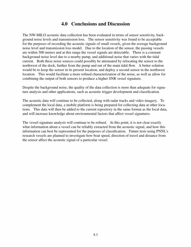
4.0 Conclusions and Discussion
The NW-MILO acoustic data collection has been evaluated in terms of sensor sensitivity, back-ground noise levels and transmission loss. The sensor sensitivity was found to be acceptablefor the purposes of recording the acoustic signals of small vessels, given the average backgroundnoise level and transmission loss model. Due to the location of the sensor, the passing vesselsare within 500 meters and at this range the vessel signals are detectable. There is a constantbackground noise level due to a nearby pump, and additional noise that varies with the tidalcurrent. Both these noise sources could possibly be attenuated by relocating the sensor to thenorthwest of the dock, further from the pump and out of the main tidal flow. A better solutionwould be to keep the sensor in its present location, and deploy a second sensor in the northwestlocation. This would facilitate a more refined characterization of the noise, as well as allow forcombining the output of both sensors to produce a higher SNR vessel signature.
Despite the background noise, the quality of the data collection is more than adequate for signa-ture analysis and other applications, such as acoustic trigger development and classification.
The acoustic data will continue to be collected, along with radar tracks and video imagery. Tocomplement the local data, a mobile platform is being prepared for collecting data at other loca-tions. This data will then be added to the current repository in the same format as the local data,and will increase knowledge about environmental factors that affect vessel signatures.
The vessel signature analysis will continue to be refined. At this point, it is not clear exactlywhat information about a vessel can be reliably extracted from the acoustic signal, and how thisinformation can best be represented for the purposes of classification. Future tests using PNNL’sresearch vessels are planned to investigate how boat speed, direction of travel and distance fromthe sensor affect the acoustic signal of a particular vessel.
4.1


Appendix A
Data Acquisition System Schematic


Appendix A – Data Acquisition System Schematic
A.1

A.2

Appendix B
Data File Formats


Appendix B – Data File Formats
The raw acoustic data is stored in binary files, with each file containing 10 minutes worth of data.The values are raw 16-bit unsigned integer values output by the data acquisition board. Each filecontains header information that includes the sampling rate, the voltage range for converting thevalues to volts, etc. The details are given in Table B.1.
The raw data files are then used to create netCDF file containing the data and meta-data thatdescribes the collection location. This format is described in Table B.2.
Table B.1. Raw Data File Format
Position Size (bytes) Type Description
0 8 unsigned int Time of the first sample as secondsfrom Jan. 1, 1970.
8 4 long Sampling rate in Hz.
12 4 floatVoltage range; e.g. if this value is10, then the range is ± 10.
16 4 int First channel scanned, channels areindexed from 0 to 7.
20 4 int Last channel scanned.
24 40 charChannel source name, 5 chars perchannel; only the names correspond-ing to the channels scanned are valid.
64 to EOF 16-bit unsigned integer
Data; the data is written in sampleorder, i.e. the first sample from thefirst channel followed by the firstsample from the second channel, etc.
B.1

Table B.2. netCDF Data File Format
Dimensionstime (unlimited) sample indextime:title variable label stringtime:units ”seconds”time:start utc date time stringtime:start posix number of seconds since Jan. 1 1970 0:00time:start posix units ”seconds”
VariablesHPH01 16-bit scaled dataHPH01:title variable label stringHPH01:units ”scaled volts”
Global Attributestz offset local timezone offset from GMTtz offset units ”hours”site string for location where data was recordedlatitude degrees lattitude of sensorlongitude degrees longitude of sensornominal sampling rate expected sampling ratesampling rate calculated sampling ratesampling rate units ”Hz”voltage range analog-digital conversion input rangevoltage range units ”volts”
B.2