Embed Size (px)
Citation preview

4th Annual Report 2010
Aarhus UniversityDCE – Danish Centre for Environment and Energy
NER
O – 4
th Annua
l Re
po
rt 2010


NUUK ECOLOGICAL RESEARCH OPERATIONS
4th Annual Report 2010
AARHUS UNIVERSITYDCE – DANISH CENTRE FOR ENVIRONMENT AND ENERGY
AU

Title: Nuuk Ecological Research Operations Subtitle: 4th Annual Report 2010 Editors: Lillian Magelund Jensen and Morten Rasch Department of Bioscience, Aarhus University
Publisher: Aarhus University, DCE – Danish Centre for Environment and Energy URL: http://dmu.au.dk
Year of publication: 2011
Please cite as: Jensen, L.M. and Rasch, M. (eds.) 2011. Nuuk Ecological Research Operations, 4th Annual Report, 2010. Aarhus University, DCE – Danish Centre for Environment and Energy. 84 pp.
Reproduction permitted provided the source is explicitly acknowledged.
Layout and drawings: Tinna Christensen, Department of Bioscience, Aarhus University Front cover photo: The research hut in Kobbefjord, April 2010. Photo: Lillian Magelund Jensen Back cover photo: Karl Martin Iversen and Nanna Kandrup making discharge measurements at the hydrometric
station at the outlet of Badesø, April 2010. Photo: Lillian Magelund Jensen
ISBN: 978-87-92825-23-0 ISSN: 1904-0407
Number of pages: 84
Internet version: The report is available in electronic format (pdf) on www.nuuk-basic.dk/Publications and on www.dmu.au.dk
Supplementary notes: Nuuk Basic SecretariatDepartment of Bioscience, Aarhus UniversityP. O. Box 358, Frederiksborgvej 399DK-4000 Roskilde
E-mail: [email protected]: +45 87158734
Nuuk Ecological Research Operations (NERO) is together with Zackenberg Ecological Re-search Operations (ZERO) operated as a centre without walls with a number of Danish and Greenlandic institutions involved. The two programmes are gathered under the umbrella or-ganization Greenland Ecosystem Monitoring (GEM). The following institutions are involved in NERO:
Department of Bioscience, Aarhus University: GeoBasis, BioBasis and MarineBasis programmes Greenland Institute of Natural Resources: BioBasis and MarineBasis programmes Asiaq - Greenland Survey: ClimateBasis programme University of Copenhagen: GeoBasis programme The programmes are coordinated by a secretariat at the Department of Bioscience at Aarhus
University, and are fi nanced with contributions from: The Danish Energy Agency The Environmental Protection Agency The Government of Greenland Private foundations The participating institutions
Data sheet

Contents
Summary for policy makers 5Morten Rasch and Lillian Magelund Jensen
Executive Summary 6Mark Andrew Pernosky, Birger Ulf Hansen, Peter Aastrup, Thomas Juul-Pedersen, Lillian Magelund Jensen and Morten Rasch
1 Introduction 11Morten Rasch and Lillian Magelund Jensen
2 NUUK BASIC: The ClimateBasis programme 13Mark Andrew Pernosky
3 NUUK BASIC: The GeoBasis programme 19Birger Ulf Hansen, Stine Højlund Pedersen, Karl Martin Iversen, Mikkel P. Tamstorf, Charlotte Sigsgaard, Mikkel Fruergaard, Magnus Lund, Katrine Raundrup, Mikhail Mastepanov, Lena Ström, Andreas Westergaard-Nielsen, Bo Holm Rasmussen and Torben Røjle Christensen
4 NUUK BASIC: The BioBasis programme 30Josephine Nymand, Peter Aastrup, Katrine Raundrup, Magnus Lund, Kristian R. Albert, Paul Henning Krogh, Lars Maltha Rasmussen and Torben L. Lauridsen
5 NUUK BASIC: The MarineBasis programme 45Thomas Juul-Pedersen, Søren Rysgaard, Paul Batty, John Mortensen, Kristine E. Arendt, Anja Retzel, Rasmus Nygaard, AnnDorte Burmeister, Winnie Martinsen, Mikael K. Sejr, Martin E. Blicher, Dorte Krause-Jensen, Peter B. Christensen, Núria Marbà, Birgit Olesen, Aili L. Labansen, Lars M. Rasmussen, Lars Witting, Tenna Boye and Malene Simon
6 NUUK BASIC: Research projects 67
6.1 Heat sources for glacial melt in a sub-arctic fjord (Godthåbsfjord) in contact with the Greenland Ice Sheet 67John Mortensen, Kunuk Lennert, Jørgen Bendtsen and Søren Rysgaard
6.2 Dana cruise in Godthåbsfjord 68 Karen Riisgaard
6.3 The Atlantic cod (Gadus morhua) in Greenlandic waters: Past and future during climate change 68 Einar E. Nielsen, Peter Grønkjær, Mary S. Wisz, Kaj Sünksen, Rasmus Hedeholm and Nina O. Therkildsen
6.4 Developing guidelines for sustainable whale watching with special focus on humpback whales 69Tenna Boye, Malene Simon and Fernando Ugarte
6.5 Climate effects on land-based ecosystems and their natural resources in Greenland 70Mads C. Forchhammer and Erik Jeppesen

7 Disturbance in the study area 72Josephine Nymand
8 Logistics 73Henrik Philipsen
9 Acknowledgements 75
10 Personnel and visitors 76Compiled by Lillian Magelund Jensen
11 Publications 78Compiled by Lillian Magelund Jensen
12 References 80Compiled by Lillian Magelund Jensen
13 Appendix 82

4th Annual Report, 2010 5
Summary for policy makers
Morten Rasch and Lillian Magelund Jensen
The year 2010 was the fourth year of opera-tion of the fully implemented Nuuk Basic programme (including both a terrestrial and a marine component), and it was the second year with complete annual time se-ries for all sub-programmes. The 2010 fi eld season in Kobbefjord started on 7 January and continued until 16 December. During this period 36 scien-tists spend approximately 360 ‘man-days’ in the study area. In August 2010, the Minister for Sci-ence, Technology and Innovation, Char-lotte Sahl-Madsen (Denmark) and the Minister for Culture, Education, Research and Church Affairs, Mimi Karlsen (Green-land) paid a visit to the Greenland Insti-tute of Natural Resources and the Green-land Climate Research Centre. The establishment of research infrastruc-ture for Nuuk Basic was fi nalised early in 2010. The infrastructure now includes a hut with accommodation, storage and laborato-ry facilities in Kobbefjord and a number of boats for transportation between Nuuk and
the fi eld sites in Kobbefjord and Godthåbs-fjord. Aage V. Jensen Charity Foundation has generously provided all infrastructures. A number of different research projects is already using data provided by the Nuuk Basic programme. In 2010, means were funded from funding sources outside the programme to several research projects cooperating with and making use of data from the monitoring programme. Among these projects, more substantial funding were given to a Canada Excellence Research Chair (CERC) in Arctic Geo-microbiology and Climate Change at the University of Manitoba led by professor Søren Rysgaard from Greenland Climate Research Centre and a new Nordic Centre of Excellence, DEFROST, led by professor Torben Røjle Christensen from Lund Uni-versity. During 2010, the Nuuk Basic program-me had a turnover of approximately 5.8 mill. DKK.
Josephine Nymand (Greenland Institute of Natural Resources, Nuuk) briefs the ministers, Charlotte Sahl-Madsen (Minister for Science, Technology and Innova-tion, Denmark) and Mimi Karlsen (Minister for Culture, Education, Re-search and Church Affairs, Greenland), about the Nuuk Basic programme at their visit to Kobbefjord, August 2010. Photo: Peter Bondo Christensen.

4th Annual Report, 20106
Executive Summary
Mark Andrew Pernosky, Birger Ulf Hansen, Peter Aastrup, Thomas Juul-Pedersen, Lillian Magelund Jensen and Morten Rasch
Introduction
The year 2010 was the fourth year of oper-ation of the fully implemented Nuuk Basic programme (including both a terrestrial and a marine component), and it was the second year with complete annual time series for all sub-programmes.
ClimateBasis
The ClimateBasis programme gathers and accumulates data describing the climatologi-cal and hydrological conditions in Kobbe-fjord. Data are measured by two automatic climate stations (C1 and C2), two automatic hydrometric stations (H1 and H2) and three diver stations (H3, H4 and H5). The two climate stations are placed next to each other to ensure data continuity. Six-teen climate parameters are monitored and data, including two derived parameters, are stored in the database. The mean annual air temperature in 2010 was 3.4 °C, which is the highest annual air temperature measured in Kobbefjord since the start of the programme. In addition, the frost free period lasted longer than in previous years with the fi rst day with a mean air temperature above freezing oc-curring 16 days earlier than in 2008/2009 and the last day with a mean air tempera-ture above freezing occurring 31 days later than in 2007-2009. In Kobbefjord, measurement of the water level and discharge started in 2006 at H1, at H2, H3 and H4 in 2007, and at H5 in 2008. Manual measurements of discharge were in 2010 continued at H1, H3, H4 and H5. H1 and H2 are measuring throughout the year, while measurements at H3, H4 and H5 starts up in early spring when the rivers are free of snow and ice, and ends in late fall before the river freezes. In 2009, a fi nal Q/h-relation was estab-lished, incorporating discharge measure-
ments over nearly the entire recorded water level. For H2, H3, H4 and H5 there still is a lack of discharge measurements at high water levels to establish reliable Q/h-relations. For H1, which is placed at the main river in Kobbefjord, the total discharge during the hydrological year 2009/2010 was 22.9 million m3. The peak discharge in 2010 was recorded 30 August and was caused by a rain event.
GeoBasis
The 2010 season was the third full season for the GeoBasis programme with a fi eld season from May to late October. 2010 was the warmest year registered since the air temperature measurements were initiated in 1866 in Nuuk. In 2010, the annual mean air temperature reached 2.6 °C and was thereby the 12th year within the total time series with an annual mean air temperature above 0 °C. The second warmest year in the time series was 1941 with an annual mean air temperature of 0.8 °C. In 2010, the monthly mean air temperatures in May, August, September, November and December were the high-est measured during the period 1866-2010, which makes it a historically warm year. The melting of snow and ice started in the beginning of May and by mid-June, all snow on the east side of the main river outlet had melted. The ice cover melt on the lakes was approximately one month earlier than in 2009. Due to logistical pro-blems, only one snow survey was carried out in mid-April in co-operation with the ClimateBasis programme. Snow depth varied from 18 cm to 20 cm at the three soil microclimate stations and was 77 cm lower than in 2009. The micrometeorological stations in Kobbefjord confi rmed the warm climate in 2010 with a mean monthly air temperature

4th Annual Report, 2010 7
of 11.3 °C at SoilFen in August compared to 8.7 °C in 2009 and only 7.4 °C in August 2008. Even at M500 (500 m a.s.l.) the mean monthly air temperature in August was 9.0 °C in 2010 compared to 7.1 °C in 2009 and 5.4 °C in 2008. At the three automatic soil stations in the area; SoilFen, SoilEmp and SoilEmpSa the soil inter-annual variations in 2010 were quite similar to those documented in 2009 although the warmer climate in 2010 caused an average soil temperature of 3.3 °C compared to only 2.8 °C in 2009. In 2010, 61 water samples were collec-ted from late April to mid-October, which is the longest fi eld season since the initiation of the GeoBasis monitoring programme in Kobbefjord. In situ mea-surements of river water temperature, conductivity and pH were conducted along with the water sampling. The river water temperature varies through the sea-son 2010 with a minimum temperature of 1.7 °C measured 28 April and with a maxi-mum temperature of 15.8 °C measured 19 July. The conductivity shows a signifi cant decrease within the snow-melting period(April-May) to a level of 18 ± 1.5 µSc m-1, while pH shows a constant level of 6.8 ± 0.4 from April to October 2010. The temporal methane (CH4) fl ux pat-tern in 2010 was similar to the pattern observed in the two previous years with a dome-shaped peak with maximum about a month after snow melt and declining to about half of the peak maximum towards the end of the summer season (around 1 September). During autumn, the methane fl ux continued to decrease consistently in September and October. The peak summer emissions in 2010 were 4 mg CH4 m-2 h-1, which was low, compared to 8 mg CH4 m-2 h-1 in 2009 and 5 mg CH4 m-2 h -1 in 2008. The temporal variation in daily net exchange of CO2 began 14 May and conti-nued until 11 October. The period with net CO2 uptake in 2010 lasted until 18 August, which was two days later than in 2008 and nine days earlier than in 2009. During this period, the fen accumulated 65.5 g C m-2, which is 50 % higher than in 2009. The estimated net uptake period was approxi-mately 81 days in 2010 or 42 % longer than in 2009, and the maximum daily uptake reached 3.14 g C m-2 d-1 compared to 1.48 g C m-2 d-1 in 2009. In the 2010 season, the programme has been completed and major repairs have been carried out. The third full year has
provided valuable learning to ensure im-provements of the monitoring in the fol-lowing years. All methods and sampling procedures are now described in details in the manual ‘GeoBasis – Guidelines and sampling procedures for the geographical monitoring programme of Nuuk Basic’, which can be downloaded from the web-site (www.nuuk-basic.dk)
BioBasis
We now have three years of data collected by the BioBasis programme. Generally, there is a high consistency in data col-lected during the three years indicating that the data and the procedures used are reliable and sound. The year 2010 had a very early melt off. A preliminary review of data related to fl owering and plant reproductive pheno-logy indicate that 2010 was characterised by early fl owering. The general pattern is that greening of vegetation as measured by Normal-ised Difference Vegetation Index (NDVI) starts as soon as the snow has melted in the beginning of June with a peak in greenness during mid-summer (20 July-5 August) followed by a gradual decrease in greenness until the frost sets in during autumn. There are exceptions to this pat-tern: In snow patches, greening increases through the complete growing season, and Loiseleuria procumbens, Silene acaulis, and Empetrum nigrum plots have more or less constant greenness through the complete snow free season. Monitoring of Salix glauca and Eriophorum angustifolium is es-pecially useful for studying the greening process through the season while monito-ring of the evergreen Empetrum plots and the Silene and Loiseleuria plots with sparse vegetation cover are most relevant for monitoring at a longer time perspective. Measurements of the land-atmosphere exchange of CO2 (using the closed chamber technique), soil temperature, soil moisture and phenology of S. glauca have been con-ducted weekly during June-September since 2008. All plots generally functioned as sinks for atmospheric CO2 at the time of measurements, as NEE was generally negative. In May, September and October, net ecosystem exchange (NEE) fl uxes were close to zero. Similar to both 2008 and 2009, the net CO2 uptake was generally higher in C plots compared with T and S plots. The

4th Annual Report, 20108
ecosystem respiration showed a constant pattern of higher emissions in T plots com-pared with other treatments, which can be explained by warmer and drier conditions leading to increased respiration rates. Permanent plots for studying lichens, bryophytes, and fungi (basidiomycetes) were established in the monitoring area in 2010. All four arthropod pitfall-trap stations established in 2007 and two window trap stations established in 2010, were open during the 2010 season. The material is stored in 70 % ethanol at Aarhus Univer-sity. Sorting follows a scheme giving time series as quickly as possible. Three samplings of microarthropods in Kobbefjord took place in the beginning of June, August and September, respectively. Each sampling consists of two sampling occasions one week apart. The collected microarthropod data enables an identifi ca-tion of key community species. The most common bird species were snow bunting and Lapland bunting with approximately 45 territories all together. Several territories of northern wheatear were observed and twice the number of redpolls compared to 2009. This indicates that the different species indeed have a slightly different timing of territorial be-haviour. Although the total amount of sing-ing males differs between the two surveys, the distribution between the species is ap-proximately the same. As this year had an early melt off, we may have been a little late with the survey. Lake ecology is studied in two lakes: Badesø (with fi sh) and Qassi-sø (without fi sh). Nutrient levels are general-ly low in the two lakes. When comparing water temperature data logged at 2 m depth in Badesø in 2008 and 2010, a clear differen-ce emerges. In 2010, warming started ear-lier and the lakes were generally warmer throughout spring and early summer than in 2008. This led to early ice melt (ice free 20 May) and a prolonged growing season. Nu-trient levels are generally very low in both lakes, but particularly total nitrogen (TN) is very variable, ranging from 0.04 to 0.14 mg l-1 in Badesø and from 0.03 to 0.15 mg l-1 in Qassi-sø. Chlorophyll a varied notably be-tween the years of sampling, but compared to more nutrient rich lakes the variation remains within a very narrow range due to the low nutrient levels. Over the three year period chlorophyll a concentration in-creased in both Badesø and Qassi-sø.
MarineBasis
The MarineBasis programme is running on its fi fth year. Parameters are presented of sea ice conditions, physiochemical oceanography and biological studies of microscopic organisms up to the highest trophic levels. The continuous monitoring of this system will go beyond just provid-ing a better understanding of high latitude marine systems and making it possible to observe and identify effects of climatic change in these regions. Satellite imagery showed a seasonal pattern of sea ice coverage in Baffi n Bay, which was comparable to previous years. Sea ice retreated northward in spring leav-ing no signifi cant ice by mid-summer, be-fore ice started building up again from the north during autumn. Inside Godthåbs-fjord, less sea ice was observed than during most previous years, only the innermost parts of the fjord appear to have experi-enced sea ice coverage visible to satellite. Glacial ice and sea ice was exported from the fjord in seasonal bursts as it has been observed previously, but in 2010 glacial ice from Narssap Sermia fl owed unhindered out of the fjord as no sea ice was observed in front of the glacier. Thus, more icebergs reached Nuuk and fl owed out of the fjord as compared to previous years. Vertical profi les of the water column showed a warm infl ow of deep coastal water during winter followed by some of the highest temperatures and lowest salinities recorded in the surface waters during summer over the past fi ve years. This surface layer also revealed high phytoplankton biomasses in summer leading to the second highest primary production peak measured since 2005. In contrast, the spring phytoplankton bloom appears to have been less pro-nounced than generally observed, which led to a more moderate decrease in nutri-ent levels in spring than usual. Neverthe-less, nutrient exhaustion in the surface layer did subsequently take place during summer production. High pCO2 values (i.e. above atmospheric concentrations) observed during the latter part of 2009 continued into January 2010, producing the single highest recorded value du-ring the programme. Aside from another smaller peak, pCO2 values during spring were generally lower than the year be-fore, thus indicating that the fjord had regained some of its CO2 uptake capacity.

4th Annual Report, 2010 9
Phytoplankton showed a seasonal suc-cession resembling the pattern observed in all years but 2009, with diatoms dominat-ing community abundances throughout the year except during the spring bloom. Hence, Phaeocystis sp. was the most abun-dant algal species during spring bloom in all years, except in 2009 when they re-mained entirely absent. Copepods peaked a month earlier than generally observed, which coincided with the highest copepod nauplii abundance recorded during the programme. Microsetella sp. still domi-nated the copepod abundance in all but one month, when Microcalanus was most abundant. The large Calanus spp. was only present in signifi cant numbers dur-ing the spring bloom. Other zooplankton than copepods also peaked during the summer production in July. Fish larvae showed highest abundances during spring in 2006-08, while they peaked during sum-mer in 2009-10 due to a decrease in sand eel and an increase in capelin. Cod larvae were observed during spring and summer. Overall, the abundance of fi sh larvae has decreased since the start of the programme (i.e. 2006). A length section from outside the fjord (Fyllas Banke) to the inner part of the fjord showed the highest fi sh larvae concentra-tion at the entrance of the fjord (i.e. ‘Main station’) along with decreasing species diversity in the inner part of the fjord, as observed in previous years. Shellfi sh larvae were present from spring to sum-mer and sand crab (Hyas sp.) and shrimp larvae (Pandalus sp.) showed almost twice the abundance as in 2008-09. Jellyfi sh were observed during winter and early spring while comb jellies (ctenophores) were pre-sent only from summer. While the length section showed crab and shrimp larvae to be present at all stations, abundances var-ied between stations along the length sec-tion and showed a signifi cant inter-annual variation. Sinking fl uxes of particulate material followed the seasonal patterns in the pe-lagic production. Isotopic composition of the sinking material indicated a stronger terrestrial signal in autumn, likely to be caused by the higher discharge of freshwater. Total carbon sinking fl ux in-tegrated over the year was comparable to the values estimated in previous years. A large part of the organic material that reaches the sediments is consumed and mineralized, partly to be returned to the
water column as nutrients. Maximum oxygen consumption coincided with the summer peak in pelagic production and elevated temperatures, which is in contrast to most previous years where consumption peaked during the higher spring production. The energetic status of one species of sea urchin and scallop is estimated using a condition index and gonad index. Scallops showed the highest gonad index in 2007 and 2010 and sea urchins in 2007 and 2009. Conditions indexes also vary signifi cantly between years; scallops showed higher values in 2007 and sea urchins in 2009 and 2010. Inter-annual differences between species may be due to different spawning times and feeding strategies. Monitoring of the large macroalgae spe-cies Laminaria longicruris (i.e. benthic fl ora) showed some of the highest recorded blade length and biomasses since 2007. Macroalgae sampling at two sites with dif-ferent exposure, i.e. protected and exposed to sea ice in most years, does not show a consistent difference in growth rates. The time series rather do however refl ect vari-ation around an established average blade length and biomass. Two major seabird colonies near Nuuk have been monitored since 2007, while other colonies in the area have been included later. One of the major colonies (Qeqertannguit) showed num-bers of breeding kittiwakes, Iceland gulls and black-backed gull similar to previous years. This colony expe-riences egg harvesting. In 2007, no representative seabird counts were ob-tained from the Brünnich’s guillemot colony (Nunngarussuit). Surveys of Qegertannguit and four other colonies in the area seem to indicate movement of the kittiwakes and Iceland gull between the different colonies and that the four other colonies may likely prove impor-tant in the monitoring programme. A photo-identifi cation programme of humpback whales is used to estimate the minimum number of individuals entering Godthåbsfjord (i.e. out of the estimated 3000 humpback whales annu-ally feeding in West Greenland waters). Since 2007, 52 different individuals have been identifi ed, with 12 new individuals identifi ed in 2010. Hence, the population is considered an open population where individuals move in and out during dif-ferent seasons and years. While the re-

4th Annual Report, 201010
sight rate of individuals from one year to the next is rather high, the re-sight rate of individuals in all four years is lower. Moreover, individual humpback whales repeatedly revisiting Godthåbsfjord seem to have a longer annual residence time within the fjord.
Research projects
In 2010, fi ve different research projects were carried out in cooperation with Nuuk Eco-logical Research Operations. The research projects focused on different biological topics in the limnic and terrestrial compart-ment of the ecosystem. The research pro-jects are presented in Chapter 6.

4th Annual Report, 2010 11
1 Introduction
Morten Rasch and Lillian Magelund Jensen
The year 2010 was the fourth year of opera-tion of the fully implemented Nuuk Basic program-me (including both a terrestrial and a marine component), and it was the second year with complete annual time se-ries for all sub-programmes. The 2010 fi eld season in Kobbefjord started 7 January and continued until 16 December. During this period 36 scientists spend approximately 360 ‘man-days’ in the study area.
1.1 The research hut at Kobbe-fjord
The research hut at Kobbefjord was taken into use during August 2009, and only mi-nor work needed to be carried out before the construction and furnishing was com-pleted. This work was carried out in 2010. The 55 m2 hut, which was generously funded by Aage V. Jensen Charity Founda-tion, includes excellent fi eld facilities for accommodation, storage and preliminary laboratory analyses.
1.2 Funding
Nuuk Basic is funded by the Danish En-ergy Agency and the Environmental Pro-tection Agency with contributions from Greenland Institute of Natural Resources, Asiaq – Greenland Survey, Department of Bioscience at Aarhus University and University of Copenhagen. Aage V. Jensen Charity Foundation has generously pro-vided most of the necessary research infrastructure, including boats, research hut, offi ce and accommodation facilities at Greenland Institute of Natural Resources.
1.3 Greenland Institute of Natural Resources and Greenland Climate Re-search Centre
In May 2010, professor Søren Rysgaard (head of the Greenland Climate Research Centre at Greenland Institute of Natural Resources), became Canada Excellence Research Chair (CERC) in Arctic Geomicro-biology and Climate Change at the Univer-sity of Manitoba. Søren Rysgaard will hold this position in parallel with his current po-sition as director of the Greenland Climate Research Centre. This will allow for a more intense cooperation between the Greenlan-dic and Canadian polar research communi-ties. The project is strongly connected with the activities within Nuuk Basic. Late in 2010, Aarhus University launched the idea of establishing an Arctic Centre at the University. Detailed plans for the structure of the centre were still not in place by the end of 2010, but it is a wish from Aarhus University to establish a close cooperation between the centre, the University of Manitoba and the Greenland Climate Research Centre. In June 2010, professor Torben Røjle Christensen from Lund University received funding for establishment of a new Nordic Centre of Excellence called DEFROST. The overall objective of DEFROST is to improve our understanding of how the carbon exchange with the cryosphere (permafrost, snow and sea ice) is affected by climate change. Focus is on key cryospheric components such as land, freshwater and ocean sy-stems; components that individually have substan-tial potential for changing ecosystem-climate feedback mechanisms. The project is strongly connected with the activities within Nuuk Basic.

4th Annual Report, 201012
In August 2010, the Minister for Science, Technology and Innovation, Charlotte Sahl-Madsen (Denmark) and the Minister for Culture, Education, Re-search and Church Affairs, Mimi Karlsen (Greenland) paid a visit to the Greenland Institute of Natural Resources and the Greenland Climate Research Centre. Following the visit to the Institute, the Ministers and their entourage visited Kob-befjord where a presentation was given of the monitoring programme ‘Nuuk Basic’. The Ministers also had the opportunity to speak with students associated with the programme and to visit the new research hut, which came into use in August 2009.
1.4 International cooperation
Nuuk Ecological Research Operations has been involved in the ongoing interna-tional work with the overall purpose of establishing a Sustaining Arctic Observing Network (SAON), an initiative approved by Arctic Council. Many bottom-up driven initiatives are taken for establishment of observing platforms to become compo-nents of a future SAON. Greenland Ecosystem Monitoring is involved in two of the larger initiatives, i.e. Svalbard Integrated Arctic Earth Ob-serving System (SIOS) and International Network for Terrestrial Research and Monitoring in the Arctic (INTERACT). SIOS is a network of different organisa-tions working with earth observations on Svalbard and in its nearest surrounding. INTERACT is a programme launched by the network SCANNET (a circumarctic network of 32 terrestrial fi eld stations) to coordinate their activities. Both pro-jects received funding through the EU 7th Framework Programme in 2010, and will be launched in the beginning of 2011. A major component of the project is a Trans-national Access programme allowing each of the participating stations (in Greenland there are four research stations participat-ing in INTERACT) to fund the stay of for-eign EU-scientists at the research stations. Greenland Ecosystem Monitoring has a relatively limited role in SIOS but a signifi -cant role in the leadership of INTERACT together with Abisko Scientifi c Research Station.
1.5 Further information
Further information about the Nuuk Ecological Research Operations (NERO) programme is collected in previous annual reports (Jensen and Rasch 2007, 2008 and 2009). Much more information is available on the NERO website: www.nuuk-basic.dk including manuals for the different monitoring programmes, a database hold-ing data from the monitoring, up-to-date weather information, a NERO bibliogra-phy and a collection of public outreach papers in PDF-format.
The NERO programme’s address is:
Nuuk Basic SecretariatDepartment of Bioscience, Aarhus UniversityP.O. Box 358Frederiksborgvej 399DK-4000 RoskildePhone: +45 87 15 87 34E-mail: [email protected]
Greenland Institute of Natural Resources provides the logistics in the Nuuk area,
Logistics CoordinatorGreenland Institute of Natural ResourcesP.O. Box 570Kivioq3900 NuukGreenlandPhone: +299 55 0 562E-mail: [email protected]

4th Annual Report, 2010 13
2 NUUK BASIC
The ClimateBasis Programme
Mark Andrew Pernosky
The ClimateBasis programme gathers and accumulates data describing the cli-matological and hydrological conditions in Kobbefjord. Two automatic climate stations (C1 and C2), two automatic hy-drometric stations (H1 and H2) and three diver stations (H3, H4 and H5) monitor all physical parameters necessary to describe the variations in climate and hydrology. Location of the different stations can be seen in fi gure 2.1. ClimateBasis is operated by Asiaq – Greenland Survey.
2.1 Meteorological data
In 2010, the climate stations in Kobbefjord were visited once by Asiaq technicians and six times by other Asiaq personnel. The maintenance of the stations included refe-rence tests of important parameters, and re-placement of the following sensors at both stations: RVI, PAR, Net Radiation (Lite) and the four component net radiometer (CNR1). A full description of the climate stations are given in Jensen and Rasch 2008.
C1C1
C2C2
C1
C2
H1H1H1
H2H2H2
H3H3H3
H4H4H4
H5H5H5
0 4 km2
N
Stream
Glacier
Lake
Land
Climate station
Discharge site
Hydrometric station
Kobbefjord drainage basin
Smaller drainage basin
Figure 2.1 Location of the climate (C1, C2), hy-drometric (H1, H2) and diver stations (H3, H4, H5) in Kobbefjord together with the drainage basins of Kobbefjord and the drainage basin for the hy-drometric stations and the diver stations.

4th Annual Report, 201014
During 2010, further work was made to facilitate automatic data retrieval from Nuuk. The system could not be made o-perational during 2010. It is planned that the system will become operational in August 2011, which will directly improve the data resilience for all connected stations (C1, C2, H1 and some stations run by GeoBasis). During the quality control of the mete-orological data, it was discovered that the air temperatures measured at both climate stations were 0.8 °C too low according to seven reference tests since the beginning of the programme and according to a com-parison with the hydrometric station H1. Data has been corrected back to 2007 and therefore the air temperatures reported
here will differ from the ones reported in previous years. The corrected data has been sent to the Nuuk Basic database at Aarhus University, Department of Bioscience.
Meteorological data 2010This annual report describes the third full year of data for all climate parameters and refers to data collected in the period from 1 January to 31 December 2010. Figure 2.2 gives an overview of selected meteorologi-cal parameters in 2010. The annual mean of recorded air tem-peratures in 2010 was 3.4 °C, table 2.1. The coldest month was March with an ave-rage temperature of -4.5 °C and minimum temperature as low as -17.4 °C. The warm-
1 Jan 1 Feb 1 Mar 1 Apr 1 May 1 Jun 1 Jul 1 Aug 1 Sep 1 Oct 1 Nov 1 Dec
Win
d di
rect
ion
(deg
ree)
Win
d sp
eed
(m s
–1)
Out
g. S
W r
ad.
(W m
–2)
Inc.
SW
rad
.(W
m–2
)N
et r
adia
tion
(W m
–2)
Sno
w d
epth
(m)
Air
pres
sure
(hP
a)R
elat
ive
hum
idity
(%)
Air
tem
pera
ture
(°C
)
2010
0–10–20–30–40100
80604020
01050
1025
1000
975
600
400
200
0
1000800600400200
0800
600
400
200
030
20
10
0360
270
180
90
0
1.2
0.8
0.4
0
Figure 2.2 Variation of se-lected climate parameters in 2010. From above: Air temperature, relative humidity, air pressure, snow depth, net radia-tion, incoming short wave radiation, outgoing short wave radiation, wind speed and wind direction. Wind speed and direction are measured 10 m above terrain; the remaining pa-rameters are measured 2 m above terrain.

4th Annual Report, 2010 15
est month was August with temperatures averaging 11.7 °C. However, the maximum temperature occurred on 2 September measuring 22.3 °C. Compared with the climate normal for Nuuk (1961-90), the re-corded temperatures in Kobbefjord during 2010 were above normal for the entire year (Cappelen et al. 2001). The general weather pattern from Janu-ary to March 2010 was characterized by long periods with NE winds and gene-rally warm, unstable temperatures rang-ing from -17 °C to 9 °C. Occasional storms brought stronger winds from the WNW and precipitation. Although every day in February measured a minimum tempera-ture below 0 °C, only 11 days measured a maximum temperature below 0 °C and only 1 day measured a minimum tempera-ture below -10 °C. After a period of nearly nine days in the end of January and begin-ning of February with temperatures above 0 °C, the snow pack at the climate stations was reduced to a mere six cm. Due to litt-le precipitation throughout the month of February, snow levels did not rise above eight cm until the end of the month. In general, 2010 had little snow cover as compared to previous years. The average temperature in March was 7.2 °C warmer than in March 2009, table 2.2. Spring came early to Kobbefjord and the last day with a mean air temperature below the freezing point was recorded on 28 April, which is on average 16 days earlier than in 2008 and 2009. The
dominant wind continued to come from NE during April and May and precipita-tion increased in May with 94.7 mm as opposed to only 33.8 mm in April. In May, the average temperature was 6.8 °C warmer than in May 2009. In June, the dominant wind direction changed to a westerly wind. This conti-nued throughout July and changed slight-ly to come out of the WSW during August. Air pressure remained high and stable throughout the entire summer. Although the mean air temperatures were above
Table 2.1 Monthly and annual mean values of selected climate parameters for 2010. For 2010 also mean relative humidity, snow depth, annual mean temperature, mean air pressure, accumulated precipitation and mean wind speed.
Month2010
Rel. hum.(%)
Snow depth(m)
Air temp.( °C)
Air pressure(hPa)
Precip.(mm)
Wind (m s-1)
Max 10 min. wind (m s-1)
Wind dir.most frequent
January 69 0.125 -3.8 999 61.5 4.2 16.0 NE
February 66 0.074 -1.6 1010 39.8 – – –
March 69 0.147 -4.5 1005 56.7 3.4 10.6 NE
April 73 0.083 -0.1 1010 33.8 3.2 10.5 NE
May 66 0.001 7.1 1011 94.7 3.7 12.0 NE
June 71 – 8.7 1008 55.2 3.4 9.8 W
July 76 – 10.7 1005 18.2 3.0 11.2 W
August 77 – 11.7 1008 241.0 3.1 10.9 WSW
September 71 – 7.8 1001 41.1 3.4 20.5 NE
October 69 – 2.9 1001 25.6 3.2 14.3 NE
November 67 0.048 1.2 1006 101.3 4.1 19.1 ENE
December 73 0.107 0.5 1013 136.3 4.1 12.3 E
2010 71 – 3.4 1006 905.1 3.5 – –
Table 2.2 Comparison of monthly mean air temperatures 2007 to 2010 (italic text re-presents months with incomplete coverage).
Month Air temperature ( °C)
2007 2008 2009 2010
January – –12.0 –5.4 –3.8
February – –13.3 –6.1 –1.6
March – –8.3 –11.7 –4.5
April – –0.9 –3.2 –0.1
May 0.6 3.9 0.3 7.1
June 5.3 7.9 6.4 8.8
July 10.8 10.9 10.6 10.7
August 10.6 8.7 9.3 11.7
September 4.0 4.4 3.8 7.8
October –0.5 0.0 –0.6 2.9
November –3.5 –1.7 –7.9 1.2
December –8.7 –7.8 –2.8 0.5
Year – -0.7 -0.6 3.4

4th Annual Report, 201016
average and higher than in previous years during the winter and spring months, summer temperatures remained close to normal. In fact, since 2007 the average temperature in July has not varied more than 0.3 °C, table 2.2. As in 2009, June and July were characterized by stable weather conditions with little precipitation, a high frequency of clear sky conditions and di-urnal variations in wind speed, tempera-ture, and relative humidity. The warmest month of the year was August instead of July, as it had been for the past three years. Most of the summer had been relatively dry, but that changed in August with a total precipitation of 241 mm occurring during four events. In September, the dominant wind direction turned back to NE. A passing low pressure system dur-ing the end of September brought along precipitation followed by wind speeds up to 20 m s-1 and tempe-ratures up to 17 °C. Although this event brought the strongest winds of the year, the temperature increase was not as impressive as a spell with temperatures up to 19.2 ° C 10 October, fol-lowed by a temperature drop to 3 ° C 11 Oc-tober, with temperatures falling as quickly as 6.5 °C per hour. These types of events caused by low pressure systems are com-mon during the autumn months. However, from October to December there was only one occurrence with mean wind speeds above 15 m s-1, compared with six in 2008 and three in 2009. Throughout November and December, the dominant wind direc-tion changed slowly from NE to E.
The fi rst day in the autumn of 2010 with a mean daily temperature below 0 °C occurred on 28 October, which is on ave-rage 31 days later than during the period of 2007-2009. Snow was fi rst recorded at the climate stations on 6 November but was gone again on 21 November due to warm temperatures and rain. Snow did not return until 10 December, which was also the start of the permanent snow cover at the climate stations. The levels of selected radiation pa-rameters are displayed in table 2.3. The vegetation underneath the radiation masts greened much sooner than during 2009, with the fi rst daily Normalised Differen-tial Vegetation Index (NDVI) value above 0.2 occurring 23 April 2010, as opposed to 5 June in 2009. The maximum greenness was measured in August with a NDVI value of 0.36. The period with positive month mean net radiation was April to September, which is a month longer than in both 2008 and 2009.
2.2 River water discharge
Hydrometric stations
In 2010, hydrological measurements were carried out at fi ve sites in the Kobbefjord area. Two hydrometric stations were e-stablished in 2007, and divers are each year deployed in three minor rivulets to Kobbe-fjord. The drainage basins of the fi ve loca-tions cover 58 km2 corresponding to 56 % of the 115 km2 catchment area to Kobbefjord.
Table 2.3 Monthly mean values of selected radiation parameters in 2010.
Month 2010 NDVI Albedo Short wave rad Long wave rad. Net rad. PAR UVB
in (W m–2) out (W m–2) in (W m–2) out (W m–2) (W m–2) (µmol s–1 m–2) (mW m–2)
January 0.00 0.66 4.6 3.0 250 284 –31.6 11.6 0.2
February 0.04 0.29 17.5 5.5 249 294 –32.4 44.0 0.9
March –0.09 0.79 69.5 53.3 256 283 –9.6 165 3.9
April 0.04 0.35 170 58.1 270 313 73.3 379 12.0
May 0.25 0.13 204 30.2 298 351 120 457 19.8
June 0.31 0.14 211 31.9 319 368 130 468 25.8
July 0.34 0.15 211 33.7 327 384 120 468 23.3
August 0.36 0.14 140 21.8 338 376 79.0 309 14.3
September 0.30 0.14 93.3 14.9 305 349 34.6 204 7.2
October 0.22 0.14 22.5 3.5 283 317 –14.9 53.1 1.8
November 0.14 0.46 6.3 3.7 281 306 –22.0 15.9 0.3
December 0.08 0.69 1.8 1.3 288 304 –16.4 4.7 0.1

4th Annual Report, 2010 17
In fi gure 2.1, the location of the hydro-metric stations (H1, H2) and the diver stations (H3, H4, H5) can be seen. For fur-ther descriptions of the stations and their respective drainage area, see Jensen and Rasch 2008 and 2009.
Q/h-relationManual discharge measurements have been carried out at station H1, H3, H4 and H5 (respectively 6, 8, 10 and 5 times) during 2010. The purpose is to establish a stage-discharge relation (Q/h-relation). It is generally recommended to base a Q/h-relation on a minimum of 12-15 dis-charge measurements covering the water levels normally observed at the station (ISO 1100-2, 1998). For H2, H3, H4 and H5 not enough discharge measurements have been made, especially at high water levels, to produce reliable Q/h-relations. Therefore, data from these stations are not presented. In 2009, a new Q/h-relation was calcu-lated based upon 17 discharge measure-ments, fi gure 2.3. For further description of the Q/h-relation, see Jensen and Rasch 2010. All of the discharge measurements made during ice free conditions in 2010 are in good accordance with the Q/h-relation. By the end of 2010, 12 discharge mea-surements have been carried out while the outlet was affected by ice and/or snow. These measurements are not included in the Q/h-relation. However, it has been observed that the Q/h-relation estimates discharge during conditions with ice and snow very well, except during heavy thaw and rain events. As a result, the Q/h-relation has been used during the winter
months to estimate discharge. While these results are considered a good estimate, they still should be used with care.
River water discharge at H1Figure 2.4 shows data from 2010. In 2010, the period with ice/snow free conditions at the outlet was approximately from 20 April to 11 November, and again from 21 November to 10 December. Discharges cal-culated beyond this period are estimated. The total discharge from H1 during the hydrological year 2009/2010 was 22.9 million m3, which is 42 % lower than in 2008/2009 and 30 % lower than in 2007/2008. The total discharge cor-responds to a runoff of 739 mm when assuming that the drainage basin covers 31 km2. The majority of the snow pack melted and drained through the river dur-ing the fi rst 15 days of May. June and July were relatively dry months with little vari-ation in discharge. Due to a very wet Au-gust, two high peaks occurred during the month with the peak discharge recorded 30 August and caused by a rain event. Due to a warm autumn, discharge levels did not drop signifi cantly below 0.5 m3 s-1 until 1 November. Discharge steadily dropped to 0.2 m3 s-1 by 20 November. On 21 November, water levels began rising again due to warm temperatures and rain-fall that completely melted the snow pack in low lying areas. This caused discharge to peak at 4.4 m3 s-1 on 3 December. As colder temperatures returned to Kobbe-fjord around 6 December, discharge levels steadily decreased to 0.4 m3 s-1. A comparison of discharge with preci-pitation has been made for the hydrologi-
Q/h-relation for H1, from 20 June 2006
Q = 33.54(h-98.68)1.8947
98.6
98.7
98.8
98.9
99.0
99.1
99.2
99.3
0 1 2 3 4 5 6 7 8 9 10 11 12Discharge Q (m3 s-1)
Sta
ge h
(m
rel
.)
Q/h-relation Measurements used in Q/h-relation Measurements, not used
Figure 2.3 Discharge - water level relation curve (Q/h-relation) at the hy-drometric station H1. The coeffi cient of correlation (R2) for the curve is 0.998.

4th Annual Report, 201018
cal year 2009/2010. The precipitation at the meteorological stations, C1 and C2, was 832 mm while the runoff from H1 equalled 739 mm. There can be many reasons for the difference between pre-cipitation and runoff. Although the Q/h-relation provides estimates of runoff dur-ing ice and snow conditions, there remains uncertainty. Other factors to take into consideration are diffi culties in measuring
precipitation (the technical aspect and geo-graphic distribution), glacial runoff and evaporation. In addition, there is a need for more knowledge of the hydrological processes in Kobbefjord. In 2011, it is hoped that hy-drological modelling of the catchments in Kobbefjord (using the new digital elevation model) will provide more insight into winter discharges at the different measuring sites.
Dis
char
ge (
m3
s-1)
Acc
umul
ated
dis
char
ge (
mill
. m3 )
0
3
6
9
12
15
18
1Jan
29Jan
26Feb
26Mar
23Apr
21May
18Jun
16Jul
13Aug
10Sep
8Oct
5Nov
3Dec
31Dec
0
6
12
18
24
30
36Manual discharge measurements
Discharge
Accumulated discharge
Figure 2.4 River water dis-charge at H1 during 2010.
Karl Martin Iversen ma-king discharge measure-ments at the hydrometric station at the outlet of Badesø, April 2010.Photo: Lillian Magelund Jensen.

4th Annual Report, 2010 19
3 NUUK BASIC
The GeoBasis Programme
Birger Ulf Hansen, Stine Højlund Pedersen, Karl Martin Iversen, Mikkel P. Tamstorf, Charlotte Sigsgaard, Mikkel Fruergaard, Magnus Lund, Katrine Raundrup, Mikhail Mastepanov, Lena Ström, Andreas Westergaard-Nielsen, Bo Holm Rasmussen and Torben Røjle Christensen
The GeoBasis programme provides long-term data of climatic, hydrological and physical landscape variables describing the environment in the Kobbefjord drai-nage basin close to Nuuk. GeoBasis was in 2010 operated by the Department of Geography and Geology, University of Copenhagen, in collaboration with the Department for Arctic Environment, Na-tional Environmental Research Institute, Aarhus University. In 2010, GeoBasis was funded by Danish Ministry for Climate and Energy as part of the environmental support programme DANCEA – Da-nish Cooperation for Environment in the Arctic. A part-time position is placed in Nuuk at Asiaq - Greenland Survey. The GeoBasis programme includes monitoring of the physical variables within snow and ice, soils, vegetation and carbon fl ux. The programme runs from 1 May to the end of October with some year-round measure-ments from automated stations. The 2010 season is the third full season for the GeoBasis programme. In 2007, the fi eld programme was initiated during a three-week intensive fi eld campaign in August in which most of the equipment was installed. Methods and sampling pro-cedures are described in detail in the ma-nual ‘GeoBasis - Guidelines and sampling procedures for the geographical monitor-ing programme of Nuuk Basic’, which can be downloaded from (www.nuuk-basic.dk/news/geobasis_manual/) Data collected by the Danish Meteoro-logical Institute shows that 2010 is the warmest year registered since air tempera-ture mea-surements were initiated in 1866 in Nuuk. In 2010, the annual mean air tem-perature reached 2.6 °C and is thereby the 12th year within the total time series with an annual mean air temperature above 0 °C. The second warmest year in the time series is 1941 with an annual mean air tempera-ture of 0.8 °C (Carstensen and Jørgensen, 2011). In fi gure 3.1, the monthly minimum,
mean and maximum air temperature for the period 1866-2010 measured at Nuuk are compared with the monthly mean air temperatures for 2010. During the period, 2010 had the maximum monthly mean air temperature in May, August, September, November and December. This makes 2010 a historically warm year.
3.1 Snow and ice
Snow cover extent
The fi rst three automatic cameras were installed in 2007 at 300 and 500 m a.s.l. to monitor the snow cover extent in the central parts of the Kobbefjord drainage basin. In September 2009, the last two snow monitoring cameras K5 and K6 were installed. Both cameras were installed at position N64 °9’06.25’’ W51 °20’46.47’’ 770 m a.s.l. (fi gure 3.2). K5 monitors Qassi-sø in the northern valley of the drainage basin while K6 is facing south monitoring the central parts of the drainage basin with Badesø and Langesø. One of the main advantages of camera-based snow monitoring is that it is relatively insensitive to cloud cover (in contrast to satellite-based techniques). Only low clouds and foggy conditions can make the image
-25
-20
-15
-10
-5
0
5
10
15
Jan Feb Mar Apr May Jun Jul Aug Sep Oct Nov Dec
2010
Air
tem
pera
ture
(°C
)
MaxMeanMin2010
Figure 3.1 The monthly minimum, mean and maximum air temperature for the period 1866-2010 measured at Nuuk (lines solid and dashed) and monthly mean air temperature for 2010 (points) (Carstensen and Jørgensen, 2011).

4th Annual Report, 201020
data unsuitable for mapping purposes. A new updated and more user-friendly algo-rithm for snow cover monitoring has been developed in MatLab, so it is now possible, for each melting season, to construct snow cover depletion curves for user specifi ed re-gions of interest (ROI) based on image data obtained at daily frequency. Figure 3.3 show the results for three ROI at respectively 200, 250 and 300 m a.s.l. seen from camera K2. The ROI at 300 m a.s.l. is facing west against the dominating wind direction which cause a smaller snow accumulation and an earli-er snow melt with 50 % of the snow cover melted on DOY 122 (2 May) in 2008. A more
extensive snowfall during winter and spring 2008/2009 caused a delay in the snow melt, so 50 % snow cover was fi rst reached 23 days later in 2009. The depletion curves for ROI 300 in 2010 (fi gure 3.3) indicates a snow melt very similar to 2008 – only delayed four days, and the snow cover at ROI 300 was entirely melted 10 May. The ROI’s at 200 and 250 m a.s.l. are facing to the north, which causes a leeward accumulation of snow and a later snow melt due to a shade effect from the surrounding mountains. On 14 May most of the area was covered with a very shallow snow cover, which delayed the snow melt with 2-3 days.
1382
0 m a.s.l.
Stream
Fjord and lake
GeoBasis stations
SoilFenSoilFen
SoilEmpSoilEmpSoilEmpSaSoilEmpSaMain St.Main St.
Carbon gasCarbon gas
Flux stationsFlux stations
Water sampling pointWater sampling point
K2_300K2_300K3_500 + K4_500K3_500 + K4_500
M1000M1000
M500M500
K5_800 + K6_800K5_800 + K6_800
Badesø Langesø
Qassi-sø
Kobbefjord
N
1 Km0
SoilFen
SoilEmpSoilEmpSaMain St.
Carbon gas
Flux stations
Water sampling point
K2_300K3_500 + K4_500
M1000
M500
K5_800 + K6_800
Figure 3.2 Location of GeoBasis stations in Kob-befjord. The base map is created from new eleva-tion and feature data.
Figure 3.3 Snow cover depletion for three regions of interest 200, 250 and 300 m a.s.l. has been analysed using a new snow cover algorithm. The regions are specifi ed on the image to the left, and the depletion curves for each region are shown in the diagram to the right. DOY= day of year. For ROI 300 the snow depletions for all three years are also shown and the image to the left show the area 14 May after a minor snowfall had occurred.
300 (2008)300 (2009)300 (2010)200 (2010)250 (2010)
300300
200200
250250
200
250
300
Sno
w c
over
frac
tion
0
0.2
0.4
0.6
0.8
1.0
90 120 150 180 210DOY

4th Annual Report, 2010 21
Snow coverIn 2010, the snow cover survey for Kob-befjord was carried out 15 and 16 April 2010. It describes snow depths and densi-ties at the three GeoBasis soil microclimate stations SoilFen, SoilEmp and SoilEmpSa using ground penetrating radar (GPR) and manual stake measurements (fi gure 3.4). During the winter 2009-2010 there was generally very little snow around sea level due to frequent thaw events. Due to low snow volume in April it was not pos-sible to use GPR neither at SoilEmp nor at SoilEmpSa for the snow cover survey. Instead, the snow depths were measured with manual stake measurements every 5 meters for the two stations in the sections 1-2, 1-3, 1-4 and 1-5 (fi gure 3.4). For Soil-Fen the GPR was used to measure snow depth and to determine ice layer thick-ness and peat layer thickness. In order to document the properties of the snowpack; snow pits were dug at SoilFen in point A1 and at SoilEmp in point C1 (fi gure 3.4). The examination of the snowpack included temperature profi ling, density measurements and texture description. Table 3.1 summarises the snow depth,
density and temperature results from the three stations. No snow pit was dug at SoilEmpSa due to thin snow layer. Snow temperature, density and water equivalent are therefore not available for SoilEmpSa in 2010. The texture of the snow profi le at SoilEmp is characterized as homogenous coarse grained snow. For SoilFen, the 15 cm profi le was characterized by three ho-rizons, i.e. the top 5 cm as fresh snow, in depth 5-10 cm as slush and below depth of 10 cm as ice. When comparing the snow cover survey 2010 with the snow cover survey 2009, carried out on the exact same dates (i.e.15 and 16 April), it is concluded that the average snow depth in 2010 was 77 cm lower at the three locations than in 2009. At SoilEmp and SoilFen, the average density was 17 % higher than at the same time in 2009 (Hansen et al. 2010).
Ice coverThe period with ice cover on the lakes in the Kobbefjord drainage basin was generally shorter in the winter 2009/2010 than in the previous winters (table 3.2). The break-up of the ice cover on the lakes was approximate-ly one month earlier than in 2009.
B2
B3B1
B5
B4C4
C5
A5
A4
A3
A2
A1
C1
C2
C3
0 0.5 kmN
SOILEMPSASOILEMP
SOILFEN
EDDYTOWER
KOBBEFJORDFIX
N
2
4
1 53
Soil station
50 mSnowpit
Figure 3.4 Map showing the three snow survey sites. The fi gure on the right outlines the strategy at each site.
Site Snow pit depth (cm)
Avg. density(kg m-3)
Snow depth(min-avg.-max) (cm)
Standard dev. of snow depth (cm)
Avg. snow tem-perature ( °C)
Avg. water eq. (mm)
Soil Fen (A1) 15 339 2–20–40 7 –0.3 51
Soil Empetrum Salix (B1) n.a. n.a. 7–19–68 13 n.a. n.a.
Soil Empetrum (C1) 10 366 6–17–65 14 n.a. 37
Table 3.1 Snow pit depth, average density, snow depth, average snow temperature and average water equivalent at the three soil stations (Soil-Fen, SoilEmp and SoilEmpSa) measured 15 and 16 April 2010. No snow pit was dug at SoilEmpSa.

4th Annual Report, 201022
An ice cover developed along the shore-line of Kobbefjord in mid-February 2010 but melted within the following two weeks. Thereafter, the fjord remained ice free for the rest of the winter and spring. An ice cover formed three weeks earlier on Qassi-sø (250 m a.s.l.) than on Badesø (30 m a.s.l.). The ice cover on Qassi-sø broke up ten days later than on Badesø. The difference in the period with ice cover on the two lakes is due to the difference in elevation.
MicrometeorologyTable 3.3 reports the monthly mean air temperature, relative humidity, surface temperature and soil temperature mea-sured at SoilFen during the fi eld season 2010. Since measurements began in 2007, 2010 was the year with the highest month-ly mean air temperatures measured at the SoilFen station. Figure 3.5 shows a com-parison between the monthly mean air temperatures in 2010 and the maximum and the minimum monthly mean air tem-peratures from SoilFen in 2007-2010. Note that data for November and December 2010 are not yet available and therefore not included. The unusual high monthly mean air temperatures are not caused by local factors within the drainage basin of Kobbefjord (fi gure 3.1).
For 2007-2010, the minimum monthly mean air temperature is –13.5 °C measured at SoilFen in February 2008, while the maximum is 11.3 °C measured in August 2010 (table 3.3). For the micrometeorological station M500, monthly mean air temperature, relative humidity, surface temperature and shortwave irradiance are presented in table 3.4. For 500 m a.s.l., the pattern of higher monthly mean air temperature for 2010 is confi rmed. In general, the monthly mean air temperatures for 2010 are higher than in 2008 and 2009 except for June and July in which the highest monthly mean air temperatures were registered in 2008. Note that the monthly mean incoming shortwave irradiance for May-August 2010 was lower than in the same months in 2008 and 2009.
3.2 Soil
Physical soil properties
The results of selected parameters for the soil stations SoilFen, SoilEmp and SoilEmpSa are presented in tables 3.3, 3.5 and 3.6. The difference in soil properties between the three locations, which were detected in 2009, is also seen in the data col-lected in 2010 (i.e. higher winter soil tem-peratures at SoilFen than at SoilEmp and SoilEmpSa). The results of the measured soil water content show markedly lower values for the well-drained soil at SoilEmp than at SoilEmpSa. The monthly mean soil moisture was 13 % at SoilEmp and 35 % at SoilEmpSa during the fi eld season 2010. The monthly mean soil temperature in depth –1 cm (surface temperature) mea-sured at SoilEmp in April-October in 2010 are higher than in 2009 which corresponds with the higher monthly mean air tempera-tures measured at SoilFen in 2010.
Table 3.2 Visually estimated dates for perennial formation of ice cover and dates for break-up of ice cover on selec-ted lakes within the Kobbefjord drainage basin and on Kobbefjord in 2009 and 2010. Data for Langesø is missing for the fi eld season 2009/2010. *Due to low cloud cover, it was not possible to estimate the exact date for break-up of the ice cover on Kobbefjord in 2010.
Break-up Formation Break-up
Badesø 13 June 2009 1 November 2009 14 May 2010
Langesø 11 June 2009 – –
Qassi-sø 22 June 2009 10 October 2009 24 May 2010
Kobbefjord 4 June 2009 12 February 2010 Between 15 Feb and 6 March 2010*
-25
-20
-15
-10
-5
0
5
10
15
Jan Feb Mar Apr May Jun Jul Aug Sep Oct Nov Dec
2010
Air
tem
pera
ture
(°C
)
MaxMin2010
Figure 3.5 Monthly mean air temperatures in 2010. Max and Min are maximum and minimum monthly mean air tempe-ratures from 2007-2010. Data from November and December 2010 are not yet available and therefore not included in this fi gure.

4th Annual Report, 2010 23
Month-year Air temp.2.5 m( °C)
Rel. hum.2.5 m(%)
Surface temp.0 m( °C)
Soil temp. –1 cm
( °C)
Soil temp. –10 cm
( °C)
Soil temp. –30 cm
( °C)
Soil temp. –50 cm
( °C)
Soil temp. –75 cm
( °C)
2007
August 7.6 84.1 7.6 9.0 9.8 10.1 8.6 7.4
September 3.8 70.1 1.9 3.4 4.3 5.3 5.9 5.8
October –0.5 64.6 –4.8 –0.6 0.2 1.1 2.3 2.8
November –3.5 74.2 –7.1 –0.3 –0.2 0.4 1.2 1.7
December –8.9 71.8 –13.1 –0.2 –0.2 3.0 0.9 1.3
2008
January –12.1 73.2 –16.0 –0.3 –0.1 0.3 0.8 1.2
February –13.5 73.1 –15.7 –0.3 –0.1 0.2 0.7 1.0
March –8.8 75.0 –11.5 –0.3 –0.1 0.2 0.7 1.0
April – – – – – – – –
May – – – – – – – –
June – – – – – – – –
July – – – – – – – –
August 7.4 76.6 7.6 9.3 9.2 8.6 8.4 7.6
September 4.1 77.8 3.9 4.7 5.2 5.9 6.0 6.0
October –0.1 69.3 –2.4 0.1 0.9 2.6 2.9 3.5
November –1.9 79.8 –4.4 –0.1 0.2 1.3 1.6 2.1
December –8.1 71.8 –11.9 –0.2 0.1 1.0 1.2 1.6
2009
January –5.5 67.6 –10.1 –0.2 0.1 0.9 1.1 1.4
February –6.2 69.3 –10.7 –0.3 0.0 0.7 0.9 1.2
March –12.0 73.7 –16.8 –0.5 –0.1 0.6 0.7 1.1
April –3.4 78.8 –6.7 –0.2 –0.1 0.5 0.7 1.0
May 0.3 71.7 –3.3 0.0 0.0 0.5 0.7 1.0
June 6.3 76.6 7.2 7.0 4.7 2.6 2.3 2.0
July 10.2 72.1 13.1 14.3 12.7 8.7 7.8 6.3
August 8.7 77.2 10.1 10.8 10.6 9.1 8.6 7.7
September 3.5 73.9 2.9 3.9 4.7 5.8 5.9 5.9
October –0.7 69.2 –3.2 –0.2 0.5 2.2 2.5 3.1
November –8.1 74.2 –13.6 –0.3 0.0 1.1 1.4 1.9
December –2.9 61.0 –8.7 –0.6 –0.2 0.8 1.0 1.5
2010
January –3.8 71.1 –7.0 –1.9 –1.0 0.5 0.7 1.1
February –1.6 67.7 –5.4 –3.2 –2.3 0.1 0.3 0.8
March –4.5 69.8 –7.9 –2.2 –1.8 –0.2 0.1 0.5
April –0.1 74.1 –3.0 –0.5 –0.5 –0.1 0.1 0.4
May 6.9 68.8 6.9 6.2 2.3 0.0 0.1 0.4
June 8.6 73.6 10.7 10.9 7.8 1.0 0.8 0.7
July 10.2 78.2 12.6 13.8 12.1 7.9 6.9 5.5
August 11.3 79.8 11.7 12.6 11.9 9.7 9.0 7.9
September 7.4 73.4 6.5 7.3 7.7 7.7 7.6 7.2
October 4.7 68.8 2.4 2.5 3.3 4.7 5.0 5.3
Table 3.3 Air temperature, relative humidity, surface temperature and soil temperature at fi ve depths (1 cm, 10 cm, 30 cm, 50 cm and 75 cm) from the SoilFen station in the fen area, from August 2007 to October 2010.

4th Annual Report, 201024
Soil water
Ninety soil water samples were collected from the soil water stations at SoilEmp and SoilFen during the period 27 May-4 October 2010. pH, temperature and con-ductivity measurements were carried out on the samples at the research hut in
Kobbefjord. In August 2010, laboratory equipment was installed in the research hut, which further enabled analyses of soil water alkalinity. The results of soil water chemistry analyses will be reported in the 2011 Annual Report.
Table 3.4 Air temperature, relative humidity, surface temperature and shortwave irradiance measured at the M500 station from January 2008 to September 2010. (Data from October to December are not yet retrieved).
Month-year Air temp. 2.5 m( °C)
Rel. Hum.2.5 m(%)
Surface temp. 0 m( °C)
Shortwave irradiance2.5 m
(W m–2)
2008
January –14.3 78.5 –16.3 6.7
February –15.6 78.1 –17.3 30.3
March –10.7 83.5 –12.3 77.2
April –2.4 67.2 –4.6 172.5
May 2.4 73.2 3.5 237.0
June 5.9 72.1 8.7 295.1
July 8.9 64.3 10.5 253.7
August 5.4 80.1 6.3 157.7
September 0.1 90.0 –0.7 74.0
October –3.2 77.6 –6.2 38.2
November –5.0 91.4 –6.2 8.5
December –10.8 82.2 –13.0 3.3
2009
January –7.7 72.0 –11.4 6.9
February –8.1 69.7 –11.8 30.1
March –13.1 76.5 –16.1 95.1
April –5.3 83.9 –7.6 166.9
May –2.5 79.9 –3.1 254.2
June 3.4 83.2 5.5 220.8
July 8.8 67.8 11.0 287.7
August 7.1 74.2 7.7 188.5
September –0.2 84.4 –1.2 82.8
October –3.6 74.9 –6.4 44.6
November –9.2 75.1 –12.2 11.8
December –3.8 57.5 –9.3 3.3
2010
January –5.5 73.8 –9.1 5.9
February –2.7 65.4 –7.5 29.6
March –6.7 73.1 –9.6 80.4
April –2.9 79.9 –5.4 170.4
May 4.6 71.3 3.8 205.6
June 5.7 79.9 7.9 211.4
July 8.5 76.3 11.2 217.8
August 9.0 81.3 8.8 132.6
September 5.6 70.9 3.2 92.7

4th Annual Report, 2010 25
River water
In 2010, 61 water samples were collected from the end of April to mid-October, which is the longest fi eld season since the initiation of the GeoBasis monitoring programme in Kobbefjord. In situ mea-surements of river water temperature, con-ductivity and pH were carried out along with the water sampling. The measured
values are presented in fi gure 3.6. The river water temperature varies through the 2010 season as it did during the 2009 season (Hansen et al. 2010) with a minimum tem-perature of 1.7 °C measured 28 April and a maximum temperature of 15.8 °C mea-sured 19 July 2010. The conductivity shows a signifi cant decrease within the snow melting period (April-May) to a level of
Month–year Soil temp.–1 cm( °C)
Soil temp.–5 cm( °C)
Soil temp.–10 cm
( °C)
Soil temp.–30 cm
( °C)
Soil moist.–5 cm(%)
Soil moist.–10 cm
(%)
Soil moist.–30 cm
(%)
Soil moist.–50 cm
(%)
2009
January –0.9 –0.7 –0.5 –0.1 2 12 4 3
February –1.3 –1.1 –1.0 –0.5 1 9 2 2
March –2.5 –2.3 –2.2 –1.7 1 7 1 1
April –1.4 –1.4 –1.3 –1.1 1 8 1 1
May 0.0 0.0 0.0 0.0 14 21 15 14
June 7.4 7.0 6.7 5.6 32 45 40 41
July 12.4 11.8 11.5 10.4 9 35 14 12
August 10.3 10.1 10.0 9.5 3 17 4 3
September 4.0 4.4 4.6 5.0 6 26 6 5
October –0.5 –0.3 –0.1 0.4 12 25 17 15
November –1.5 –1.3 –1.1 –0.4 2 13 3 3
December –1.9 –1.8 –1.7 –1.2 1 10 2 2
2010
January –5.2 –5.1 –4.9 –3.9 1 8 2 2
February –5.3 –5.1 –5.0 –4.1 1 8 1 2
March –4.5 –4.4 –4.4 –3.9 1 8 1 2
April –0.6 –0.8 –0.8 –0.8 6 16 10 8
May 6.4 5.6 5.1 3.8 19 42 34 31
June 10.1 9.4 9.0 7.7 5 35 8 5
July 12.4 11.8 11.4 10.4 4 28 5 4
August 11.6 11.3 11.2 10.6 11 37 15 15
September 7.0 7.3 7.4 7.6 9 38 14 11
October 2.8 3.2 3.4 4.0 6 37 6 5
Table 3.5 Soil temperature and soil moisture at four depths measured at SoilEmp from January 2009 to October 2010.
20
15
10
5
0
28
26
24
22
20
18
16
7.2
6.8
6.4
6.0Apr May Jun Jul Aug Sep NovOct Apr May Jun Jul Aug Sep NovOct Apr May Jun Jul Aug Sep NovOct
2010 2010 2010
A B C
pH
Con
duct
ivity
(µS
c m
–1)
Wat
er te
mpe
ratu
re (
°C)
Figure 3.6 River water temperature (A), conduc-tivity (B) and pH (C) mea-sured in Kobbefjord River at the water sampling point near the research hut in 2010.

4th Annual Report, 201026
18 ± 1.5 µSc m-1. From the beginning of June and through the rest of the fi eld season, the conductivity shows no signifi cant trend. pH shows a constant level of 6.8 ± 0.4 from April to October 2010.
3.3 Vegetation
Vegetation in the Kobbefjord area is moni-tored by both the BioBasis and GeoBasis programmes. While BioBasis monitors in-dividual plants and plant phenology using plot scale sites and transects, the GeoBasis programme monitors the phenology of the vegetation communities from satellite.
Satellite imageryAcquisition of satellite imagery for a spe-cifi c date can be diffi cult since the satellite have to pass on the given day under cloud free conditions. Therefore, the satellite companies allow only for ordering of ima-
gery from a given minimum period (e.g. three weeks) and not a specifi c date. When the conditions of cloud free acquisition are met, the fi rst time during this period, the task is done and no further acquisitions performed. In 2010, the conditions for a suc-cessful acquisition were met on 10 July i.e. a week earlier than the images from 2008 and 2009 and around three weeks earlier than the time of maximum growth (see section 4.1). The reasons for inter-annual differences between greenness are therefore diffi cult to access although a comparison will give an indication. A QuickBird multispectral image with 2.4 m resolution was acquired and geo-rectifi cation performed. Dark subtraction was carried out as the atmospheric correc-tion but without topographic correction. Normalised Difference Vegetation Index (NDVI) has been calculated on the imagery from 10 July 2010. An NDVI image covering the main part of the monitoring area is shown in fi gure 3.7.
Month–year Soil temp.–1 cm( °C)
Soil temp.–5 cm( °C)
Soil temp.–10 cm
( °C)
Soil temp.–30 cm
( °C)
Soil moist.–5 cm(%)
Soil moist.–10 cm
(%)
Soil moist.–30 cm
(%)
Soil moist.–50 cm
(%)
2009
January – – –0.3 0.2 37 27 41 38
February – – –1.1 –0.3 15 13 33 32
March – – –1.4 –0.7 13 12 12 25
April – – –0.4 –0.2 15 13 13 14
May – – 0.0 0.0 30 21 17 16
June – – 4.1 3.5 59 52 38 35
July – – 11.0 9.5 51 42 45 45
August – – 10.2 9.1 40 30 38 33
September – 5.3 5.0 5.5 – 32 38 33
October 0.4 0.9 0.8 1.0 60 53 44 48
November –0.4 0.2 0.0 0.3 52 37 41 42
December –0.7 –0.2 –0.4 –0.1 28 21 38 35
2010
January –1.7 –1.0 –1.4 –0.5 23 14 19 34
February –2.6 –1.8 –2.2 –1.3 21 13 12 22
March –1.9 –1.7 –1.8 –1.4 20 12 11 12
April –0.2 –0.3 –0.3 –0.3 26 15 12 13
May 3.1 1.3 1.7 1.0 59 47 26 17
June 8.3 6.0 6.8 5.5 60 46 47 46
July 11.4 9.7 10.6 9.2 56 32 42 38
August 11.0 10.2 10.4 10.1 59 49 44 45
September 7.6 7.7 7.6 7.7 60 49 46 49
October 3.8 4.6 4.1 4.9 58 37 44 45
Table 3.6 Soil temperature and soil moisture at four depths measured at SoilEmpSa from January 2009 to October 2010.

4th Annual Report, 2010 27
The areas on the imagery represent fi ve different vegetation types from the area: fell fi eld, open mixed heath, Empetrum dominated heath, fen and copse. Figure 3.8 shows the difference in NDVI for the fi ve vegetation types in 2008, 2009 and 2010 (Notice that images are not topographically corrected and that date of acquisition is outside the maximum green-ness peak). The fell fi eld areas had a much higher NDVI in 2010 than in previous years, though direct comparison is diffi cult due to the different dates of the images.
3.4 Carbon gas fl uxes
Carbon gas fl uxes are monitored on plot and landscape scale in a fen area using two different techniques:
• Automatic chamber measurements of the CH4 and CO2 exchange on plot scale
• Eddy covariance measurements of the CO2 and H2O exchange on landscape scale
Automatic chamber measurementsAn automatic chamber system consisting of six fl ux chambers for monitoring of the exchange of CH4 and CO2 (see fi gure 3.11) was installed in August 2007 (Tamstorf et al. 2009). In 2010, the system was operated from 14 May until 11 October. Gaps in data originate from maintenance, calibra-tion and malfunction due to various errors such as fox bites and instrument failures. The spatial and temporal variation in CH4 emissions (fi gure 3.9) is primarily
NDVI
0.70 - 0.80
0.60 - 0.70
0.50 - 0.60
0.40 - 0.50
0.30 - 0.40
0.20 - 0.30
0.10 - 0.20
0.05 - 0.10
0.00 - 0.05
Non-veg.
0 2.5 km Figure 3.7 Normalised Dif-ference Vegetation Index (NDVI) based on QuickBird imagery from 10 July 2010. Data are dark sub-tracted as atmospheric correction and lack the topographic correction.
0
0.2
0.4
0.6
0.8
Fell field Openmixed heath
Empetrumdom. heath
Fen Copse
Vegetation type
ND
VI
200820092010
Figure 3.8 NDVI for the fi ve vegetation types from 17 July 2008 and 2009, and 10 July 2010. Notice that changes between greenness are due not only to phenology differences between years but also seasonal phenology as the image is acquired approxi-mately 2 weeks before the maximum greenness and on different dates.

4th Annual Report, 201028
related to temperature, water table depth and net primary production. The fen in Kobbefjord is a source of CH4 due to the permanently wet conditions that promote anaerobic decomposition, by which CH4 is an end product. In 2010, measurements started earlier than in previous years, allowing monitor-ing of CH4 emissions before onset of the growing season. During May, fl uxes were fairly constant ranging 1-3 mg CH4 m-2 h-1. The observed overall temporal CH4 fl ux pattern in 2010 was similar to the patterns observed in 2008 and 2009; i.e. low shoul-der season emissions and a dome-shaped peak with a maximum in July. Peak sum-mer emissions, approximately 4 mg CH4 m-2 h-1, were lower than those observed in 2009 but in the same range as those observed in 2008. The peak summer CH4 emissions from the fen in Kobbefjord are comparable to the emissions in a fen in Zackenberg, NE Greenland.
Eddy covariance measurements
In order to describe the seasonal CO2 ba-lance, the soil-atmosphere CO2 exchange in a fen has been monitored using the eddy covariance technique since 2008. The eddy covariance system consists of a 3D sonic anemometer and a closed path infrared CO2 and H2O gas analyzer (Tamstorf et al. 2009). Raw data from the eddy covariance systems were calculated using the software package EdiRe (Robert Clement, University of Edinburgh). For more details on the fl ux calculation procedures see Hansen et al. 2010. The temporal variation in the mean diurnal net ecosystem exchange of CO2 (NEE) and air temperature during 2010 for the fen site is shown in fi gure 3.10, and various variables are summarised in table 3.7. NEE refers to the sum of all CO2 exchange processes; including photosyn-thetic CO2 uptake by plants, plant respira-tion and microbial decomposition. The
2010
Met
hane
flux
(m
g C
H4
m–2
h–1
)
0
2
4
6
8
10
14 May 29 May 13 Jun 28 Jun 13 Jul 28 Jul 12 Aug 27 Aug 30 Aug 11 Sep 26 Sep 11 Oct
Figure 3.9 Methane (CH4) emissions from the fen during 2010.
−2
−3
−1
0
1
2
−20
−30
−10
0
10
20
100 140 180 220 260 300
NEE
TairNet
eco
syst
em e
xcha
nge
(g C
m–2
d–1
)
Air tem
perature (°C)
DOY
Figure 3.10 Diurnal net ecosystem exchange (NEE) and air temperature (Tair) measured in the fen in 2010.

4th Annual Report, 2010 29
CO2 uptake is controlled by climatic con-ditions, mainly temperature and photo-synthetic active radiation (PAR), whereas respiratory processes are controlled main-ly by temperature, soil moisture and the amount of biomass. The sign convention used in fi gures and tables is the standard for micrometeorological measurements; fl uxes directed from the surface to the at-mosphere are positive, whereas fl uxes di-rected from the atmosphere to the surface are negative. Eddy covariance measurements of the CO2 and H2O exchange in the fen were initiated 4 May and lasted until 9 October. During this period, 5 % of data were lost due to malfunction, maintenance and calibration. Early in the season, before plants began photosynthesising, small CO2 emissions were measured. Maximum spring diurnal emission was measured 7 May, amounting to 0.57 g C m-2 d-1. As the vegetation developed, the photosynthetic uptake of CO2 started, and 29 May the fen ecosystem switched from being a net source to a net sink of atmospheric CO2. This is the earliest onset of net uptake pe-riod measured so far. The period with net CO2 uptake in 2010 lasted until 18 August (table 3.7), which was in between 2008 (16 August) and 2009 (27 August). During this period, the fen accumulated –65.4 g C m-2, and the maxi-mum daily accumulation rate amounted to –3.1 g C m-2 (measured 1 July). These are the highest accumulation rates mea-sured so far, likely associated with the early snow melt and onset of growing season period. By 18 August, respiration processes exceeded the fading photo-synthesis, and the ecosystem returned to a net source of atmospheric CO2. In the beginning of this period, there is plenty of fresh litter available and soil temperatures remain comparably high, allowing decom-position processes to continue at a decent rate. Highest autumn diurnal emission was measured 27 August (1.53 g C m-2 d-1). During the entire measuring period (158 days), the total CO2 accumulation amount-ed to –20.9 g C m-2.
Table 3.7 Summary of the measuring periods and CO2 exchanges for 2008-2010 at the fen site. Please note that the measuring period varies from year to year.
Year 2008 2009 2010
Measurements start 5 Jun 15 May 4 May
Measurements end 29 Oct 31 Oct 9 Oct
Start of net uptake period – 1 Jul 29 May
End of net uptake period 16 Aug 27 Aug 18 Aug
NEE for measuring period (g C m-2) –45.5 –14.0 –20.9
NEE for net uptake period (g C m-2) – –42.5 –65.4
Max. daily accumulation (g C m-2 d-1) –2.27 –1.48 –3.14
Figure 3.11 Eddy covariance mast and automatic chambers for measurement of GHG exchange in the Kobbefjord area. Photo: Morten Rasch.

4th Annual Report, 201030
4 NUUK BASIC
The BioBasis programme
Josephine Nymand, Peter Aastrup, Katrine Raundrup, Magnus Lund, Kristian R. Albert, Paul Henning Krogh, Lars Maltha Rasmussen and Torben L. Lauridsen
This chapter presents the results of the fourth year of the BioBasis monitoring programme at Nuuk. The chapter gives an overview of the activities and presents some examples of the results. The pro-gramme aims at providing long-term data series on biotic variables from the Kobbe-fjord area. A thorough statistical analysis will follow when we have longer time series. Methods and sampling procedures are described in detail in the manual ‘Con-ceptual design and sampling procedures of the biological programme of Nuuk Ba-sic’ (Aastrup et al. 2009). The programme was initiated in 2007 by the National Environmental Research In-stitute, Aarhus University, in cooperation with the Greenland Institute of Natural Resources. BioBasis is funded by the Envi-ronmental Protection Agency as part of the environmental support programme DAN-CEA – Danish Cooperation for Environ-ment in the Arctic. The authors are solely responsible for all results and conclusions presented in this chapter, which do not necessarily refl ect the position of the Envi-ronmental Protection Agency.
4.1 Vegetation
Reproductive phenology
We followed the reproductive phenology of three plant species (Silene acaulis, Salix glauca, and Loiseleuria procumbens) in plots established in 2007/08. For each species, four phenology plots were set up to cover the ecological amplitude of the species with respect to snow cover, soil moisture, and altitude. The fi rst visit to the plots in 2010 was 28 April. Snow melt was very early and some of the plots were already free of snow. In addition, at this occasion, many of the plots were heavily impacted by larvae of the noc-tuid moth, Eurois occulta. Loiseleuria procumbens budding and fl owering in 2010 occurred earlier than seen in previous years. The time for 50 % fl owering occurred up to three weeks earlier than in 2009 (fi gure 4.1), while the time for peak fl owering occurred more than one month earlier this year compared to 2009, which so far was the year with the latest fl owering (fi gure 4.2A). The se-quence of fl owering by plot was the same as in previous years with plot Loi4 being the earliest followed by plot Loi1, Loi2, and Loi3. Flowering in Silene acaulis peaked around 9 June (fi gure 4.2B), at the same time as we expect that the number of Eu-roris occulta larvae peaked. The true peak would probably have been later if the moths had not been there. The time of 50 % fl owering in Sil4 was approximately two weeks earlier in 2010 than in 2009 and ap-proximately one week earlier than in 2008 (fi gure 4.1). This plot was the one with least signs of larvae attack at the time of fl ower-ing. We were not able to record counts of 50 % fl owers in plot Sil1, Sil2 and Sil3 be-cause a high proportion of the buds were eaten just before fl owering. The date of 50 % fl owers seems to have been between
DO
Y
200820092010
0
50
100
150
200
250
300
Loiseleuriaprocumbens
Salix glauca (f) Salix glauce(hair)
Silene acaulis
Figure 4.1 Mean value day of year (DOY) of 50% fl owers for each of the species (Loiseleuria procumbens, Salix glauca, and Silene acaulis) in the plant reproductive phenology plots for 2008, 2009 and 2010. Also included are the senescent fl owers in Salix glauca.

4th Annual Report, 2010 31
2 June and 8 June. It seems that there was a high degree of synchrony among the plots in 2010 as was also the case in 2009. We did see new buds later in the season but only few of these reached fl owering. The phenological progression in female fl owers in Salix glauca occurred almost three weeks earlier in 2010 than in 2009 (Sal2 and Sal3) (fi gure 4.3A and B), while the progression of formation of hairs was only 10 to 15 days earlier (fi gure 4.1). It seems that the timing of ‘hairing’ takes place within a relatively short period of time by the end of September, indepen-dent of the timing of fl owering. In all three years, the female fl owering has exhibited a similar pattern with a steep rise in fl ower-ing followed by a long period of 50 to 90 days with a constantly high proportion of fl owers. In plot Sal1, we recorded almost no buds or fl owers because leaves and buds were eaten by the noctuid larvae E. occulta. The plants suffered severely until the beginning of August when new green leaves appeared. We did not record any new buds or fl owers.
Phenology of Salix glauca in CO2-fl ux plots In 2010, Salix glauca produced female fl ow-ers in only eight CO2-fl ux plots. In all but one plot Salix glauca specimens produced less than 10 female buds. Most buds were produced in Temperature manipulated plot 3 (3T), but most fl owers were pro-duced in the Short Growing season plot 2 (2SG). In 2010, only this plot and the Long Growing season plot 2 (2LG) produced fl owers with hairs indicating that most of the fl owers in the other plots did not pro-duce mature seeds, were eaten, or fell off before reaching maturity. Figure 4.4 shows an example of the phenology in a CO2-fl ux plot (4C).
Total fl oweringTotal counts of fl owers were only carried out in the Eriophorum angustifolium plots, and in Loiseleuria plot number 4. Due to the larvae outbreak of Eurois occulta most of the buds and fl owers in the remaining plots were eaten before total counts could be made. The fl owering of Eriophorum was at the same level as during the two previous years. However, plot 4 had much more
110 140 170 200 230 260 290 110 140 170 200 230 260 290
70
60
50
40
30
20
10
0
80
60
40
20
0
DOYDOY
Flo
wer
s (%
)
Flo
wer
s (%
)
2008
2009
2010
A B
Figure 4.2 The progression in phenology shown as the percentage of fl owers by day of year (DOY) in 2008, 2009 and 2010. A: Loiseleuria procumbens B: Silene acaulis. Percentages have been averaged over plots.Erratum: Figure 4.2A in NERO 3rd Annual Report (Jensen and Rasch 2010) is not correct. Data has now been recalculated and is shown correctly in the present report.
100
80
60
40
20
0
100
80
60
40
20
0
DOYDOY
Flo
wer
s (%
)
Hai
rs (
%)
2008
2009
2010
A B
140 170 200 230 260 290 140 170 200 230 260 290
Figure 4.3 Salix glauca fl owers (A) and senescent fl owers (B) in 2008, 2009 and 2010 averaged over all plots.

4th Annual Report, 201032
fl owers than the other plots. Loiseleuria plot 4 had less than a fourth of the number of fl owers counted in 2009, probably due to the larval outbreak.
Summing up reproductive plant phenologyThe year 2010 had a very early melt-off of snow. A preliminary review of data related to fl owering and plant reproductive pheno-logy indicate that 2010 was characterised by:• Early fl owering• Two budding events in Loiseleuria
procumbens and Silene acaulis• A high impact of noctuid moth, Eurois
occulta
• Low seed production compared to the two previous years as a consequence of many buds and fl owers being eaten by the noctuid moth, Eurois occulta larvae.
Vegetation greening, NDVIWe followed the greening of the vegeta-tion in Empetrum nigrum ssp. hermaphrodi-tum plots, in plant phenology plots and along the NERO line. We used a handheld Crop Circle TM ACS-210 Plant Canopy Refl ectance Sensor, which calculates the greening index (Normalized Difference Vegetation Index – NDVI). Measurements were made weekly in the E. nigrum plots and in the plant phenology plots, and monthly along the NERO line (Bay et al. 2008).
NDVI in Empetrum nigrum and plant phenology plotsAs in the two previous years, vegetation greening followed three different patterns depending on the species monitored. The evergreen E. nigrum (fi gure 4.5A) has no clear peak time of greenness. Plot 4, however, had a weak indication of a peak in all three years; this may be because of the presence of Salix glauca and Vaccinium uliginosum in this plot. Eriophorum angusti-folium (fi gure 4.5B) and Salix glauca (fi gure
30
20
25
15
10
5
0
DOY
Flo
wer
s (%
)
140 170 200 230 260 290
2008
2009
2010
Figure 4.4 Salix glauca fl owers in the CO2-fl ux control plot 4C in 2008, 2009 and 2010.
Figure 4.5 Average NDVI values during the season indicated by day of year (DOY). A: Empetrum nigrum (plot 1). B: Eriophorum angustifolium (plot 1). C: Salix glauca (plot 2). D: Loiseleuria procumbens (plot 3). E: Silene acaulis (plot 2).150 170 190 210 230 250 270 290 150 170 190 210 230 250 270 290
150 170 190 210 230 250 270 290
0.7
0.6
0.5
0.4
0.3
0.2
0.1
0.7
0.6
0.5
0.4
0.3
0.2
0.1
DOY DOY
DOY
Ave
rage
ND
VI
Ave
rage
ND
VI
2009
2008
2010
A C
E
B
D

4th Annual Report, 2010 33
4.5C) exhibited more or less bell-shaped greening curves, except for plot Sal1, which to some degree fl uctuated, probably because of the loss of leaves due to the E. occulta larvae. Loiseleuria procumbens plots have sparse vegetation, and greening only showed weak time dependence (fi gure 4.5D). One plot had a weak bell shaped curvature (Loi3). Silene acaulis plots gave the lowest NDVI-values through all sea-sons independent of day of year (fi gure 4.5E).
NDVI along the NERO lineThe NERO line (Bay et al. 2008) covers eight vegetation types (dwarf shrub heath, snow patch, herb slope, fen, copse, Des-champsia-Juncus community, lake and pond vegetation, and salt marsh). Vegeta-tion greenness is measured monthly along a line 5 m north of the NERO line. Figure 4.6 shows the results from parts of the NERO line representing four vegetation types. In copse, fens and heaths, we see more or less bell shaped greenness curves with a similar or slightly later greening in 2010 compared to 2008 and 2009.
Summing up – vegetation greeningAfter only three years of monitoring ve-getation greening by NDVI, we have still no fi rm conclusions. Generally, data ap-
pear consistent and reliable, and we see some tendencies that will be interesting to follow in the future and in comparison with equivalent data from Zackenberg, NE Greenland and other monitoring sites. The general pattern is that greening starts as soon as the snow has melted in June with a peak in greenness in mid-summer (20 July-5 August) followed by a gradual decrease in greenness until the frost sets in during autumn. There are ex-ceptions to this pattern: • In snow patches greening increases
through the complete growing season.• Loiseleuria procumbens, Silene acaulis,
and Empetrum nigrum plots have more or less constant greenness through the whole snow free season.
Monitoring of S. glauca and E. angusti-folium is considered useful for studying the greening process through the season, while monitoring of the evergreen Em-petrum plots, and the Silene and Loiseleuria plots with sparse vegetation cover are most relevant for monitoring at a longer time perspective.
Carbon dioxide exchangeIn 2008, a manipulation experiment was initiated with fi ve different treatments, each with six replicates. The experiment is located
150 170 190 210 230 250 270 290150 170 190 210 230 250 270 290
0.8
0.7
0.6
0.5
0.4
0.3
0.2
0.8
0.7
0.6
0.5
0.4
0.3
0.2
DOYDOY
Ave
rage
ND
VI
Ave
rage
ND
VI
2008
2009
2010
A
C
B
D
Figure 4.6 NDVI measure-ments along the NERO line represented for four vegetation types in 2008, 2009 and 2010. A: Copse. B: Fen. C: Dwarf shrub heath. D: Snow patch vegetation. For location of the different vegetation types please see Jensen and Rasch 2010.

4th Annual Report, 201034
in a mesic dwarf shrub heath dominated by Empetrum nigrum with Salix glauca as a subdominant species. Treatments include control (C), shortened growing season (SG: addition of snow in spring), prolonged growing season (LG: removal of snow in spring), shading (S: hessian tents) and in-creased temperature (T: ITEX Plexiglas hexa-gons). We have conducted measurements of land-atmosphere exchange of CO2 using the closed chamber technique, soil temperature, soil moisture and phenology of Salix glauca approximately weekly during June-October in each year. The net ecosystem exchange (NEE) was measured with a transparent chamber while the ecosystem respiration (Reco) was measured with a darkened cham-ber. The SG and LG treatments have not been applied in 2008-2010, so results from these plots can be considered as controls.
The fi rst CO2 fl ux measurement day in 2010 was 25 May (the area was snow free early this year). Until the last measure-ment day (11 October), CO2 fl uxes were measured in all plots on 18 occasions. All plots generally functioned as sinks for atmospheric CO2 at the time of measure-ments, as NEE was generally negative (fi -gure 4.7). In May, September and October, NEE fl uxes were close to zero. Similar to both 2008 and 2009, the net CO2 uptake was generally higher in C plots compared with T and S plots. The ecosystem respira-tion showed a constant pattern of higher emissions in T plots compared with other treatments, which can be explained by warmer and drier conditions leading to in-creased respiration rates. The highest rates of gross primary production (GPP: diffe-rence between NEE and Reco) were gene-rally observed in C plots, while especially S plots showed lower GPP rates compared with other treatments. As photosynthesis is driven by solar radiation, shading de-creases GPP and build-up of biomass. These results are in general similar to those obtained in 2008 and 2009.
UV-B exclusion plotsMeasurements of chlorophyll fl uorescence as a measure of plant stress were carried out in Kobbefjord in 2010. The impact of ambient UV-B radiation on the vegetation is studied in a mesic dwarf shrub heath dominated by Empetrum nigrum and with Betula nana and Vaccinium uliginosum as subdominant species. The experimental UV-B set-up reduces the UV-B infl ux by approximately 60 % (Mylar fi lm) and this is compared to a control fi lm (Tefl on), which is UV-B and PAR neutral, and an open control. The exclusion plots were set up by the end of May, and besides periods with spells of strong winds the treatments were maintained until the mid to end of August. The ambient UV-B radiation on fl uore-scence parameters were monitored on Vac-cinium and Betula. The total performance index (PItotal, integrating responses of antenna, reaction centre, electron transport and end acceptor dependent parameters) meaning an indicator of a samples via-bility, were sensitive to UV-B exclusion in both Betula and Vaccinium. The average PItotal was improved by around 8 % in Vac-cinium and around 14 % in Betula when reduced UV-B was compared to near ambient UV-B (table 4.1). The PItotal was
NE
E (
mg
CO
2 m
–2 h
–1)
Rec
o (m
g C
O2
m–2
h–1
)G
PP
(m
g C
O2
m–2
h–1
)
−1000
−800
−600
−400
−200
0
200C SG LG S T
0
100
200
300
400
500
JunMay Jul Aug OctSep–1400
–1200
–1000
–800
–600
–400
–200
0
2010
Figure 4.7 Monthly means of net ecosystem exchange (NEE: upper panel), ecosystem respira-tion (Reco: middle panel) and gross primary produc-tion (GPP: lower panel) in 2008, 2009 and 2010 in the manipulation ex-periment plots. Error bars refer to standard error in spatial variability (six repli-cates). Negative fl uxes in-dicate CO2 uptake by the ecosystem, while positive fl uxes indicate CO2 release to the atmosphere.

4th Annual Report, 2010 35
signifi cantly decreased 27 July but not 6 August in Betula (fi gure 4.8). In Vaccinium the PItotal were improved 27 July, but not 29 July and 6 August when UV-B was reduced compared to near ambient UV-B (fi gure 4.8).
Permanent lichen plotsAt the end of June 2010, 13 permanent li-chen monitoring plots were established in Kobbefjord by Eric Steen Hansen, Natural History Museum of Denmark, University of Copenhagen. The aim of the study was to establish permanent plots for long-term monitoring of lichen communities. The monitoring plots were established in close connection to the NERO Line. Each plot consists of 10 replicate plots perpendicular to the NERO Line 2 m apart. Each repli-cate was analysed with Raunkjær vegeta-tion analyses. Additionally 22 permanent lichen plots were established, 12 epilithic lichens and 10 epigaeic lichens, in order to follow the increase or decrease of growth in these specifi c lichens. The total number of lichens species recorded is 114, which is less than the 160 species recorded for the surroundings of Nuuk. One reason may be that the comparatively short time spent in the area did not allow for all interesting lichen sites to be thoroughly investigated.
Permanent bryophyte plots
At the end of August 2010 seven perma-nent bryophyte monitoring plots were es-tablished in Kobbefjord by Kristian Hassel and Tommy Prestø, Norwegian University of Science and Technology, Museum of Natural History and Archaeol-ogy, Trondheim, Norway. The aim of the study was to establish permanent plots for long term monitoring of bryophyte communities. The monitoring plots were established 3-5 m northeast of the NERO Line. Each plot consists of fi ve replicates plots 5 m apart along a straight line paral-lel to the NERO Line. Each of the replicate
2010 Parameter C F B P-value
Betula nana FV/FM 0.77±0.007B 0.768±0.007B 0.79±0.006A 0.008
RC/ABS 0.589±0.011AB 0.571±0.013B 0.62±0.017A 0.0127
ET0/TR0 0.512±0.011A 0.472±0.012B 0.52±0.013A 0.0014
RE0/ET0 0.583±0.008A 0.617±0.014A 0.58±0.014A 0.0395
PIabs 2.47±0.21B 2.08±0.15B 3.04±0.27A 0.0003
PItotal 3.42±0.28B 3.61±0.29AB 4.2±0.35A 0.0747
Vaccinium uliginosum
FV/FM 0.82±0.004A 0.815±0.004A 0.817±0.003A 0.5494
RC/ABS 0.617±0.008A 0.581±0.007B 0.607±0.008A 0.0002
ET0/TR0 0.673±0.004A 0.642±0.006B 0.652±0.006B 0.0001
RE0/ET0 0.53±0.005A 0.531±0.004A 0.522±0.005A 0.0012
PIabs 6.17±0.21A 4.96±0.18C 5.49±0.23B 0.0001
PItotal 7.06±0.27A 5.7±0.24B 6.18±0.34B 0.0001
Table 4.1 The chlorophyll fl uorescence parameters were analyzed with the OJIP test approach (Strasser et al. 2004). The parameters: The ratio of PSII reaction centre’s (RC) and absorbance fl ux, [RC/ABS]. The maximum quantum yield, [φPo = FV/FM)] which corresponds to the effi ciency an absorbed photon will be trapped by PSII RC leading to QA reduction. The fraction of electrons transported beyond QA-per exiton trapped by the open reaction PSII RC, [ψEo = ETo/TRo]. The effi ciency with which an electron can move from the reduced intersystem electron acceptors to the PSI end acceptors, [δRo = REo/ETo]. The performance index [PIabs = (RC/ABS) × [φPo/(1-φPo)] × [ψEo/(1-ψEo)] × [δRo/(1-δRo)]]. The total performance index integrating the responses of antenna, reaction centre, electron trans-port and end acceptor dependent parameters [PItotal = (RC/ABS) × [φPo/(1-φPo)] × [ψEo/(1-ψEo)] × [δRo/(1-δRo)]]. The presented values are the seasonal mean ± standard error for open control (No fi lter), Filter Control (near ambient UV-B, Transparent fi lter, Tefl on), UV-B reduction (UV-B absorbing fi lter, Mylar). Analysis of variance included effects of block, campaign (C), treatment (T) and the interaction CxT and the P-values for treatment are given. Tukey test different letters indicate differences between means tested with the test, (p < 0.05).
27 July 29 July 6 August27 July 6 August0
2
4
6
8
10
UV-B reductionFilter controlOpen control
Tot
al p
erfo
rman
ce in
dex
(PI to
tal)
Betula nana Vaccinium uliginosum
Figure 4.8 Seasonal variations in total perfor-mance index for Betula nana and Vaccinium ul-iginosum. The values are mean ± standard error for Open control (no fi lter) Filter control (transparent fi lter, Tefl on) and UV-reduction (UV-B absorbing fi lter, (Mylar). B. nana was measured only twice while V. uliginosum was mea-sured three times.

4th Annual Report, 201036
plots were pin point analysed using a frame of 70 cm × 70 cm with 100 pins. Each species hit by the pin through the vegeta-tion layer were monitored. Lichens were recorded as a functional group as were graminoids, herbs, woody plants, detri-tus and club mosses. Additionally, a free search within the plots as well as between the plots, were undertaken to register presence of additional species, as the pin point method tends to miss rare species. The collection is currently being exa-mined, but so far, 215 taxa of bryophytes have been identifi ed.
Permanent basidiomycetes plots In mid-August 2009, twenty-four perma-nent basidiomycetes monitoring plots were established in Kobbefjord by Thorbjørn Borgen, Botanical Museum, University of Copenhagen, Denmark. The aim of the study was to establish permanent plots for long-term monitoring of basidiomycetes communities. The monitoring plots were established next to and parallel with the NERO Line. Each plot consists of a square measuring between 3 m² and 10 m². Each plot was intensively surveyed for fungi. The collection is currently being examined but so far 78 species of basidiomycetes have been identifi ed. As the season of 2009 was very dry and hence not optimal for fungi growth, the potential number of common taxa is expected to be higher. About 40 ad-ditional taxa are occurring in neighbouring areas (Nuuk, Paamiut, Sisimiut).
4.2 A rthropods
In Kobbefjord, all four pitfall trap sta-tions established in 2007 and two win-dow trap stations (each with two trap)
established in 2010 were open during the 2010 season. Sampling procedures follows the manual ‘Conceptual design and sampling procedures of the biologi-cal programme of Nuuk Basic’ (Aastrup et al. 2009). Part of the samples are being sorted by Department of Terrestrial Eco-logy, National Environmental Research Institute, Aarhus University, Denmark. The material is stored in 70 % ethanol at Aarhus University.
Window trapsThis was our fi rst season with window traps. We established two traps each with two trapping chambers at two different locations: At Art2 named Wart1 and Wart2 on 12 May, and at Art3 named Wart3 and WArt4 on 14 May. They worked continu-ously until the end of the season (begin-ning of October).
Pitfall trapsAll pitfall traps were established on 12 or 14 May. They all worked continuously until the end of October when their liquid began to freeze. This year we had an outbreak of insect larvae and especially of larvae of Euroris occulta. The largest number of larvae was present in the beginning of June (fi gure 4.9). Later in the season (at the end of Au-gust) we saw two other peaks of larvae other than E. occulta. The samples have not all been sorted yet, but the work is on-going at Aarhus University. The outbreaks of larvae have been known to occur every now and then. In 2010, it was reported from several places along the west coast of Greenland, more pronounced in the inland areas than in the coastal areas.
MicroarthropodsThe three samplings for microarthropods in Kobbefjord took place in the beginning of June, August and September, respec-tively. Each sampling consists of two sam-pling occasions one week apart. The soil cores are extracted at Greenland Institute of Natural Resources immediately after sampling, and the extracted microarthro-pods are stored in 70 % ethanol. After the last sampling, the specimens are shipped to Aarhus University. The population data structure as re-vealed by principal component analysis (PCA) of the correlation matrix of log(x+1) transformed population abundances is shown in fi gure 4.10.
100
80
60
40
20
0
DOY
Tot
al S
UM
140 160 180 200 220 240 260 280 300
Figure 4.9 Total number of larvae in the arthropod samples through the sea-son 2010.

4th Annual Report, 2010 37
The fi rst two principal components refl ect the difference between the four plant communities. Isotomiella minor, Folsomia quadrioculata, Folsomia sensibilis and Desoria olivacea contributes to the fi rst principal component (PC) axis and are common in Salix and Empetrum plots but rare in Silene and Loiseleuria plots as was also observed in 2009. Therefore, the fi rst PC axis is a habitat axis ordering the plant habitats from Loise-leuria-Silene, Empetrum Mart2, Empetrum Mart1, over Salix MArt3 to Salix MArt4. The Empetrum MArt2 plot has much more Tetracanthella arctica than MArt1 plot. The second PC axis divides the Salix and Empetrum plots according to the dominant euedaphic Tullbergiinae and Willemia sp., which contributed to this axis. Hence, Salix MArt3 plot has more of these collembolans compared to Mart4 plot. Although it can still be questioned whether the two plots within the same habitat type are suffi cient-ly similar to be treated together, the four habitats still fall naturally into large groups.
PhenologyThe collembolan that attained the highest observed abundance, T. arctica, (table 4.2) had an exponential population growth during the season, which was signifi cant in 2009 but not in 2010. In both years of sampling the abundance of D. olivacea increased during the fi rst two months, while the common F. quadrioculata in Empetrum and Salix, MArt4 plot, did not
show any phenological trends. Folsomia sensibilis had a mid-summer minimum in both years, which in 2009 could be ex-plained by summer drought. However, in 2010 another mechanism must have been the cause. I. minor declined signifi cantly during the season in both Salix and Em-petrum plots, where it otherwise was most abundant.
EmpetrumSalixSileneLoiseleuria
Silene
Loiseleuria
SalixEm
petrum
Table 4.2 Mean abundances (× 1000 individuals m-2) of mites, at order level, and col-lembolans, at species level. Microarthropods are the sum of mites and collembolans. Shaded areas: habitat characterising key species S: Collembolan species richness; H’ = – pi log2 pi, where pi is the proportion of species in the sample to total collem-bolans; E: H/log2 n, where n is number of collembolan species.
Salix Empetrum Silene Loiseleuria
S, species richness 19 12 9 11
H', diversity index 2.8 2.7 1.2 2.1
E, evenness 0.7 0.7 0.4 0.6
Microarthropods 108 114 127 152
Acari 80.3 89 115 137
Collembola 27.8 24.8 11.8 15.1
Tullbergiinae1 6.2 2.6 8.5 4.7
Tetracanthella arctica 1.5 6.2 0.2 4.9
Willemia sp.2 4.6 1.3 2.3 3.7
Isotomiella minor 7.4 2.3 0.1 0.07
Folsomia quadrioculata 2.2 6 0.6
Folsomia sensibilis3 1 4.6 0.1 0.1
Desoria olivacea 2.3 0.8
Micranurida pygmaea 0.02 0.6 0.4 0.9
Juvenile H. claviger 0.6 0.2 0.1
Parisotoma notabilis 0.46 0.02
Desoria tolya 0.36 0.01
Onychiurinae4 0.18 0.01
Lepidocyrtus violaceus 0.04 0.12
Lepidocyrtus cyaneus 0.01 0.04
Juvenile Isotomidae5 0.03 0.01
Arrhopalites principalis 0.03
Sminthuridae6 0.025
Isotoma anglicana 0.017
Fimetaria coeruleogrisea 0.01
Pseudanurophorus binoculatus 0.01
Megalothorax minimus 0.01
Actinedida 40.4 41.2 67.5 74.7
Oribatida 33.9 45.5 46.9 59.9
Gamasida 3.9 2.1 0.2 1.1
Acaridida 0.03 0.09 0.02
1Include Mesaphorura tenuisensillata, M. jirii, M. macrochaeta, Karlstejnia norvegica2W. anophtalma and W. scandinavica3Includes other folsomids4Presumably dominated by Oligaphorura ursi but also include other Onychiurinae5Isotoma multisetis or Isotoma anglicana6A. principalis juveniles, Sminthurinus schotti and unidentifi ed Sminthurides juveniles
Figure 4.10 PCA plot of the correlation matrix of log-transformed microarthropod community samples. Each soil core sample is repre-sented by a symbol. Lines are drawn around clusters comprising the microarthropod samples within the plant communities. The broken line through the Empetrum cluster divides the cluster into the two sampling plots that were both assigned to the Empetrum plant habitat type.

4th Annual Report, 201038
Climatic trendsHitherto 2010 was the warmest and wettest season (May-August) since the beginning of the monitoring programme in 2007. The 2009 season was the driest and coldest sea-son. We compared the two years by running an ANOVA of log+1 transformed popula-tion numbers. For most of the species we found no dramatic changes except for Loise-leuria plots MArt8 and MArt7 where the Tullbergiinae and Willemis sp., respectively, were much lower in 2009 than in 2010. The eudaphic life-form is expected to be more vulnerable to drought, as they do not possess visible traits that protects against drought. In the Silene MArt6 plot and Salix MArt3 plot a similar phenomenon was ob-served for Tullbergiinae.
Future perspectiveThe collected microarthropod data are now of a quality that enables an identifi cation of key community species. As the sampling has been limited to the top 5.5 cm of the soil and førne (litter) layer some euedaphic species, i.e. collembolans living in the top of the soil and true soil dwellers, may not be represented in the dataset, which then calls for an additional sampling covering the complete vertical soil profi le. The Salix and Empetrum heath habitats harvest the most diverse communities and the largest biomass compared to the Silene and Loise-leuria habitats. The last two habitats have a low primary productivity and a sandy soil with a comparably low humus content, so we fi nd small microarthropods adapted to these conditions and with a growth poten-tial when conditions become favourable, i.e. Tullbergiinae, Willemia sp. and Actine-did mites. To gain further insight into the soil ecosystem processes of the Kobbefjord area we suggest characterizing the food web structure using natural abundance of stable isotopes. For future soil food web modelling the information about the role of species and functional guilds in proces-
sing soil organic matter and plant debris is crucial. By using stable isotope δ signatures of 13C and 15N, we can identify relationships between the composition and structure of the soil community and the ecosystem pro-cesses to which they contribute, like orga-nic matter decomposition, the emission of CO2, and the mineralisation of nutrients. So future ecosystem modelling would then be able to calculate the process rates as carried out by soil organisms and their role in pro-visioning stability of ecosystem processes. When employing δ signatures to map the trophic structures, we can detect changes in the food web structure over time as an ad-ditional indicator of ecological change. As such, trophic changes is related to the ac-tual functioning of the organisms and they may prove to be more valuable than track-ing ecosystem changes through population dynamics.
4.3 Birds
Survey for breeding passerines
The survey for breeding birds took place 1 June and 15 June following the same pro-cedure and transects as in previous years. The transects crosses 14 waypoints, and at each waypoint fi ve minutes is spent ma-king observations. Birds observed within a distance of up to 300 m from the transect were mapped on fi eld maps. Individuals of snow bunting (Plectrophenax nivalis) Lapland bunting (Calcarius laponicus) and northern wheatear (Oenanthe oenanthe) were sexed and singing activities recor-ded. Based on singing and the number of males, the numbers of territories of snow bunting and Lapland bunting were esti-mated (table 4.3). Redpolls (Carduelis fl am-mea) were not sexed. The most common species were snow bunting and Lapland bunting with ap-proximately 45 territories all together. Several territories of northern wheatear were observed and also twice the num-ber of redpolls compared to 2009. This indicates that the different species indeed have a slightly different timing of territo-rial behaviour. In 2009 there was more consistency between the two surveys com-pared to 2010; this may be explained by the longer period between the surveys in 2010. Although the total amount of singing males differs, the distribution between the species is approximately the same. As this
Table 4.3 Number of territories of Lapland bunting, snow bunting and northern wheatear within the research area. Redpolls were not sexed so we do not know the number of territories.
2009 2010
Date 2 June 8 June 1 June 15 June
Snow bunting 29 21 15 9
Lapland bunting 17 19 29 15
Wheatear 1 1 8 4
Redpoll individuals 2 5 9 5

4th Annual Report, 2010 39
year had an early melt-off, we may have been a little late with the survey.
Bird census pointsPasserine birds were counted at 13 census points during the entire season. When arri-ving at a census point fi ve minutes were used as a ‘settling period’ and a following fi ve minute period was used for counting the birds. In 2010 the fi rst observation was 17 May and the last was 6 October, so this year we had the longest period of bird counting.
Lapland buntingAs in the last two years Lapland buntings were observed at most points during the entire season except in the beginning and at the end. We observed more birds in 2010 than the previous years, but we also conducted more censuses. Knowing that there were outbreaks of insect larvae (see previous section), this may have increased the survival and number of successful breeding attempts. Most of the Lapland buntings were observed in the fjord area with the highest number in the middle of the season (end of June) (fi gure 4.11).
Snow buntingSnow bunting was the most numerous of all passerines with the highest numbers in the beginning and at the end of the season. Especially in mid-September we found a high number of snow bunting at the fjord and more inland.
RedpollIn contrast to previous years we saw red-polls during the entire season except from September. In addition, they were seen both in the fjord area and in the inner val-ley. The last observation was 4 October when one group of approximately 20 indi-viduals were clearly on migration.
Northern wheatearThe number of northern wheatear was the highest ever recorded. We have observations from the beginning of the season until the end of August. The observations are distri-buted throughout the entire census area, and both males and females were observed. However, by the end of the season the num-ber of individuals in groups tended to be higher than in the beginning of the season.
Fjord area Inner valley
DOY
Num
ber
0
5
10
15
20
25
30
147 152 159 166 173 180 189 196 202 223 228 243147 152 159 166 173 180 189 196 202 223 228 243
222174 186 198 210 225 240165 180 195 210 225 240165 180 195 210222174 186 198 210
Fjord area Inner valley
Num
ber
0
3
6
9
12
15
0
1
2
3
4
7
6
5
Fjord area Inner valley
DOY DOY
20092008
2010
Figure 4.11 Number of Lapland buntings ob-served in the fjord area (Point A-H) and in the inner fjord (Point I-M) in 2008, 2009 and 2010.

4th Annual Report, 201040
4.4 Mammals
We did not see any mammals in the Kobbe-fjord area except for Arctic fox. During the late winter and early spring we heard Arctic fox barking at several visits to Badesø but otherwise they were rarely seen. On 1 June a presumed rabies infected fox attacked and bit our boatman. The fox was shot and delivered to the authorities for examination, and it was confi rmed that it was infected with rabies.
4.5 Lakes
The BioBasis programme monitors two of four lakes in the catchment area of Kob-befjord, Badesø and Qassi-sø. They are both deep lakes with a maximum depth of 33 and 26 m, respectively. Badesø is the downstream lake situated at an altitude of 50 m a.s.l. and has an area of 80 ha. Qassi-sø is situated upstream of Badesø at an altitude of approximately 250 m a.s.l. and has an area of 52 ha. Badesø contains fi sh (Arctic char and sticklebacks), while Qassi-sø is without fi sh. A full data set from the BioBasis pro-gramme is now available for the three year period 2008-2010. Submerged ma-crophytes data are available from 2007-2010, and hourly/daily water tempera-ture data from 2008 and 2010. Fish and macroinvertebrates have been sampled once, in 2008.
TemperatureThe altitude difference between the two lakes causes a temperature difference, and the length of the ice free period consequ-ently varies. In 2007, the ice free period was 35 days longer in Badesø than in Qassi-sø (Jensen and Rasch 2010). In addition, within the lake inter-annual variations oc-curred in the ice free/ice covered periods depending on climatic conditions. The daily overview photos of the Kobbefjord catchment area illustrate the development (fi gure 4.12). In 2008, Qassi-sø was 50 % ice covered and ice free 10 and 12 June, re-spectively. In 2009 the corresponding dates were 22 and 28 June, respectively. In 2010 the corresponding dates were 24 and 31 May, respectively. From 2008 to 2009 the ice free period has shortened with 12-16 days, while from 2009 to 2010 it was prolonged by almost one month. A similar pattern was observed in Badesø (fi gure 4.13). The temperature data logged in the lakes provide similar information but also add to our knowledge on the pri-mary production capacity in the systems. The production is not only dependent on light availability and the duration of the ice free period but is also positively cor-related with temperature. When compa-ring water temperature data logged at 2 m depth in Badesø during the period 15 April to 14 June in 2008 and 2010, a clear difference between the years emerges (fi gure 4.14). In 2010, warming started earlier and the lakes were generally
Figure 4.12 50 % ice cover in Qassi-sø 10 June 2008 (A), 22 June 2009 (B), and 24 May 2010 (C). The lake was ice free 12 June in 2008, 28 June in 2009 and 20 May 2010. Photo: GeoBasis pro-gramme.
A
B
C

4th Annual Report, 2010 41
warmer throughout spring and early summer than in spring 2008. This led to an early ice melt (ice free 20 May), a pro-longed growth season and a potentially higher primary production during the growth season, either in the water phase as phytoplankton or as epiphyton at the sediment surface in areas where light reaches the bottom.
NutrientsNutrient levels are generally very low in both lakes, but particularly total nitrogen (TN) is very variable, ranging from 0.04 to 0.14 mg TN l-1 in Badesø and from 0.03 to 0.15 mg TN l-1 in Qassi-sø. In addition, total phosphorous (TP) varied widely, in particular in 2008, ranging between 0.002 and 0.008 mg l-1 in Badesø, and 0.001 and 0.025 mg l-1 in Qassi-sø (fi gure 4.15A and B). A comparison of between-year sum-mer concentrations shows that TN and TP were lower in 2009 compared to 2008 and 2010. Spring 2009 was cold and primary production started later, which may have infl uenced the TN and TP concentrations. However, only a slightly lower phytoplank-ton biomass was recorded in Badesø in 2009 (fi gure 4.19).
Chlorophyll a and suspended matterChlorophyll is correlated to nutrient le-vels and the chlorophyll a levels of the two lakes are consequently low (fi gure 4.16). Chlorophyll varied notably be-tween the years of sampling, but com-pared to more nutrient rich lakes, the variation remains within a very narrow range due to the low nutrient levels. Over the three year period chlorophyll con-centrations increased in both Badesø and Qassi-sø (fi gure 4.16). In correspondence with this the Secchi depth decreased, this being particularly pronounced in Badesø where the Secchi depth decreased from 8.2 m to 5.4 m (fi gure 4.17). In Qassi-sø we did not fi nd the same reduction in Secchi depth, probably because Secchi depth in Qassi-sø is affected by silt rather than chlorophyll. Increasing chlorophyll levels and decreasing Secchi depth are typical signs of increasing eutrophication and are an expected outcome of tempera-ture increase. It must be borne in mind, though, that our data concerns only a three year period and the results may therefore be coincidental. Future results will help clarify this.
Suspended matter includes organic and inorganic matter such as silt and clay derived from snow melt and eroded ma-terial during periods with high runoff due to, for instance, heavy rain. The close correlation between silt and Secchi depth was illustrated in Qassi-sø in September 2010 (fi gure 4.18), after several days of exceptionally heavy rain. This led to an extreme runoff and transport of silt into the lake, resulting in an very low Secchi depth of 0.5 m (fi gure 4.17).
Figure 4.13 50 % ice cover in Badesø 1 June 2008 (A), 12 June 2009 (B), and 19 May 2010 (C). The lake was ice free 3 June 2008, 15 June 2009 and 20 May 2010. The snow cover was thicker in the winter 08/09 compared to 07/08 and 09/10, as illustrated by the snow fan in front of the camera in June 2009. Photo: GeoBasis programme.
A
B
C

4th Annual Report, 201042
PhytoplanktonIn both lakes the phytoplankton biomass was completely dominated by chryso-phytes and dinophytes, species typical of oligotrophic systems. The chrysophytes did not dominate the entire year, but only from ice break up until mid-July, then dinophytes typically took over or constituted at least 50 % of the biomass. From late summer diatoms contributed signifi cantly to the biomass in Qassi-sø, but chlorophytes were important too. The low nutrient levels in 2009 are not refl ected in the phytoplankton biomass. A possible explanation is P-limitation, as known from marine waters. This theory is supported by the increasing phyto-plankton biomass during autumns 2008 and 2009 in Qassi-sø, where the TP con-centration rose as well (fi gure 4.19). Phytoplankton sampling was con-ducted following ice break in spring. This explains the abrupt appearances in fi gure 4.19. However, in 2010 the fi rst samplings in Badesø were obtained in April before ice break, showing a modest phytoplank-ton biomass and therefore, presumably, negligible primary production under the ice. Phytoplankton production due to light attenuation through the ice could have been hypostasised, but this is not supported by the results. On the other hand, the 2010 results from Badesø show a very fast appearance of algae follow-ing the ice break, illustrating the growth potential in spring when light conditions are optimized and nutrients have accu-mulated during the winter period.
VegetationAs in previous years, the submerged macrophytes community was clearly dominated by water starwort (Callitriche hamulata) and secondarily by mosses
20082010
Badesø
0
2
4
6
8
10
12
0 168 336 504 672 840 1008 1176 1344 1512Hours
Wat
er te
mpe
ratu
re (
°C)
Figure 4.14 Hourly water temperature measure-ments at 2 m depth in Badesø during spring 2008 and 2010 (from 1 am 15 April to 11 pm 14 June, both years). One week is 168 hours.
2009 20102008
Badesø
TNTP
Qassi-sø
0
0.04
0.08
0.12
0.160
0.04
0.08
0.12
0.16
2 May 1 Nov 3 May 2 Nov 4 May 3 Nov
Tot
al N
and
P (m
g l-1
)T
otal
N a
nd P
(mg
l-1)
Figure 4.15 Total nitrogen (TN) and total phosphorus (TP) concentrations during summer 2008-2010 in Badesø and Qassi-sø.
Figure 4.16 Chlorophyll a concentrations during summer 2008-2010 in Badesø (solid line) and Qassi-sø (broken line).
2009 20102008
BadesøQassi-sø
2 May 1 Nov 3 May 2 Nov 4 May 3 Nov
Chl
orop
hyll
a (µ
g l-1
)
0
0.4
0.8
1.2
1.6

4th Annual Report, 2010 43
(fi gure 4.20). In 2010, macrophyte cover-age reached its highest level in Badesø compared to the previous three years, and its second highest level in Qassi-sø. In four of six 1 m depth zones of Badesø, C. hamulata increased in coverage. In con-trast, there was a decrease in the cover-age of mosses. We do not know if mosses compete with C. hamulata, but when C. hamulata expand, mosses will invariably decline. The increase in C. hamulata cove-rage can be a response to an earlier and warmer spring in 2010 compared to 2009, improving primary production condi-tions in 2010. Figure 4.21 depicts the maximum depth limit of C. hamulata and mosses. In both lakes there were a signifi cant in-crease in the depth limit during the moni-toring period, but especially the mosses expanded extraordinarily fast towards deeper water. A depth expansion is very positive in eutrophic waters; whether a depth expansion is positive or negative in oligotrophic, clear and cold water lakes is more uncertain, however, the expansion may be due to a prolonged temperature dependent growing season. If so, the ex-pansion is induced by climatic changes and thus negative.
2009 20102008
BadesøQassi-sø
2 May 1 Nov 3 May 2 Nov 4 May 3 Nov
Sec
chi d
epth
(m
)
0
2
4
6
8
10
12
Figure 4.17 Secchi depths during summer 2008-2010 in Badesø (solid line) and Qassi-sø (broken line).
2009 20102008
2 May 1 Nov 3 May 2 Nov 4 May 3 Nov0
2
4
6
8
10BadesøQassi-sø
Sus
pend
ed m
ater
ial (
mg
l-1)
Figure 4.18 Suspended matter during summer 2009-2010 in Badesø (solid line) and Qassi-sø (broken line). No data from 2008.
Chlorophyceae
PrymnesiophyceaePrasinophyceae
Diatomophyceae
Chrysophyceae
DinophyceaeCryptophyceae
2008 2009 2010
Badesø
Qassi-sø
0
0.05
0.10
0.15
0.20
0.250
0.05
0.10
0.15
0.20
0.25
J F M A M J J A S O N D J F M A M J J A S O N D J F M A M J J A S O N D
Bio
mas
s (m
m3
l-1)
Bio
mas
s (m
m3
l-1)
Figure 4.19 Phytoplankton biomass during summers 2008-2010 in Badesø and Qassi-sø.

4th Annual Report, 201044
In view of the reduced Secchi depth dur-ing the monitoring period, a reduced macrophytes depth limit would have been expected. However, the depth limit has not reached the potential maximum depth limit at the given Secchi depth yet
(maximum depth limit = 0.07 + 1.83 × Sec-chi Depth, see Jensen et al. 1996). Conse-quently, it can be concluded that factors other than Secchi depth control the depth limit in these clear water lakes.
Dep
th li
mit
(m)
Badesø Qassi-sø
0
2
4
6
8
10
2007 2008 2009 2010 2007 2008 2009 2010
CallitricheMoss
Figure 4.21 Maximum macrophyte depth limits in Badesø and Qassi-sø from 2007-2010. Linear regres-sion lines are shown.
Depth interval (m)
Cov
erag
e (%
)C
over
age
(%)
0
10
20
30
50
40
0
10
20
30
50
40
Badesø
Qassi-sø
0–1 1–2 2–3 3–4 4–5 5–6 >6 0–1 1–2 2–3 3–4 4–5 5–6 >6
2007
2008
2009
2010
Figure 4.20 Macrophyte coverage at 1 m depth in-tervals down to 6 m from 2007-2010 in Badesø and Qassi-sø. Water starwort (Callitriche hamulata) is shown to the left and mosses to the right. Macrophyte coverage is measured once every year in August.

4th Annual Report, 2010 45
5 NUUK BASIC
The MarineBasis programme
Thomas Juul-Pedersen, Søren Rysgaard, Paul Batty, John Mortensen, Kristine E. Arendt, Anja Retzel, Rasmus Nygaard, AnnDorte Burmeister, Winnie Martinsen, Mikael K. Sejr, Martin E. Blicher, Dorte Krause-Jensen, Peter B. Christensen, Núria Marbà, Birgit Olesen, Aili L. Labansen, Lars M. Rasmussen, Lars Witting, Tenna Boye and Malene Simon
The following chapter presents results from 2010, the fi fth year of the MarineBa-sis monitoring programme in Godthåbs-fjord. The programme aims at establishing long-time series of key parameters within physical, chemical and biological oceano-graphy, along with organisms on higher trophic levels. In order to get a better un-derstanding of the marine ecosystems in arctic regions, particularly on seasonal and inter-annual variability, demands consi-stent time series. Long-time series are even more important for improving the ability to separate out natural variability in order to detect possible effects of climatic chan-ges. Monthly pelagic sampling is carried out at a ‘Main Station’ (64 °07’N, 51 °53’W) near the entrance to the Godthåbsfjord system. In addition, an annual length section is carried out from Fyllas Banke to the inner part of the fjord along with an annual cross section of the fjord, both
during May (fi gure 5.1). The programme also includes benthic sampling four times per year at a ‘Sediment Station’ in Kobbe-fjord. The annual monitoring efforts also comprise a sub-programme on benthic fl ora and fauna as well as observations on seabirds and whales. Finally, sea ice condi-tions within the fjord system and Baffi n Bay are monitored using satellite imagery and digital camera systems (Godthåbs-fjord only). Methods are briefl y described throughout the chapter. For more details please consult the MarineBasis Nuuk Manual (www.nuuk-basic.dk).
5.1 Sea ice
Sea ice conditions in Baffi n Bay are moni-tored daily using AMSR-E satellite images (3-6 km resolution, fi gure 5.2). Similar to previous years, sea ice covered much of the
NuukNuuk
Main StationMain Station
Sediment stationSediment station
Seabird colony Seabird colony (QeqertannguitQeqertannguit)
Seabird colony Seabird colony (Nunngarussuit)(Nunngarussuit)
Cross sectionCross section
Akia
Akia
Fyllas BankeFyllas Banke
Main Station
Sediment station
Seabird colony (Qeqertannguit)
Seabird colony (Nunngarussuit)
Cross section
10 km
Akia
Fyllas Banke
Nuuk
Arctic Circle
Figure 5.1 Map of sam-pling stations in and around the Godthåbs-fjord system. X represent sampling stations along the hydrographical length section.

4th Annual Report, 201046
bay until April/May when it retreated from the south, reaching a summer minimum coverage (i.e. open water) by July/August. Sea ice started building-up again from the north in September, covering the north-western part of the bay by December. Daily MODIS satellite images (250 m resolution, fi gure 5.3) showed a modest sea ice cover in the inner part of Godthåbsfjord
and smaller fjord branches, considerably less than was observed during the previous winter (i.e. 2008/2009). Sea ice in Kobbe-fjord was also limited to the innermost part of the fjord. Analyses of satellite data on sea ice coverage are currently conducted in collaboration between Greenland Institute of Natural Resources, the Danish Meteoro-logical Institute and Greenland Climate Re-
Figure 5.2 Satellite images (AQUA AMSR-E) showing sea ice extent in Baffi n Bay in February, May, August and December 2010.Blue colour represents open water and pink and yellow colours represent different sea ice conditions.
Figure 5.3 Satellite images (AQUA-MODIS) showing sea ice conditions in Godt-håbsfjord during January, May, August and Novem-ber 2010.
January
August
May
November

4th Annual Report, 2010 47
search Centre. As a courtesy, daily satellite images covering Greenland are available on www.dmi.dk. Ongoing research at the Greenland Climate Research Centre and the Danish Meteorological Institute is at-tempting to improve satellite imagery and remote sensing data for the region. Digital images are recorded every hour overlook-ing a section of Godthåbsfjord near Nuuk (fi gure 5.4). Major parts of the Godthåbs-fjord system remain largely free of ice, only experiencing periodic bursts of sea ice and glacial ice being exported out of the fjord, as it is recorded on the presented digital images. However, in 2010, glacial ice from one of the glaciers within the fjord (Narssap
Sermia) could fl ow unhindered out of the fjord as no sea ice was observed in front of the glacier. Thus more icebergs reached Nuuk and were exported out of the fjord as compared to previous years.
5.2 Length and cross sections
A cross section of Godthåbsfjord, i.e. from Nuuk to Akia (fi gure 5.1), was sampled in late-May using a SBE19+ CTD profi ler measuring salinity, temperature, density, oxygen concentration, turbidity, irradiance (PAR) and fl uorescence. Vertical profi les of salinity, temperature and fl uorescence
Figure 5.4 Digital ima-ges from Godthåbsfjord showing open water in October (A) and a burst of glacial ice in December 2010 (B).
A
B
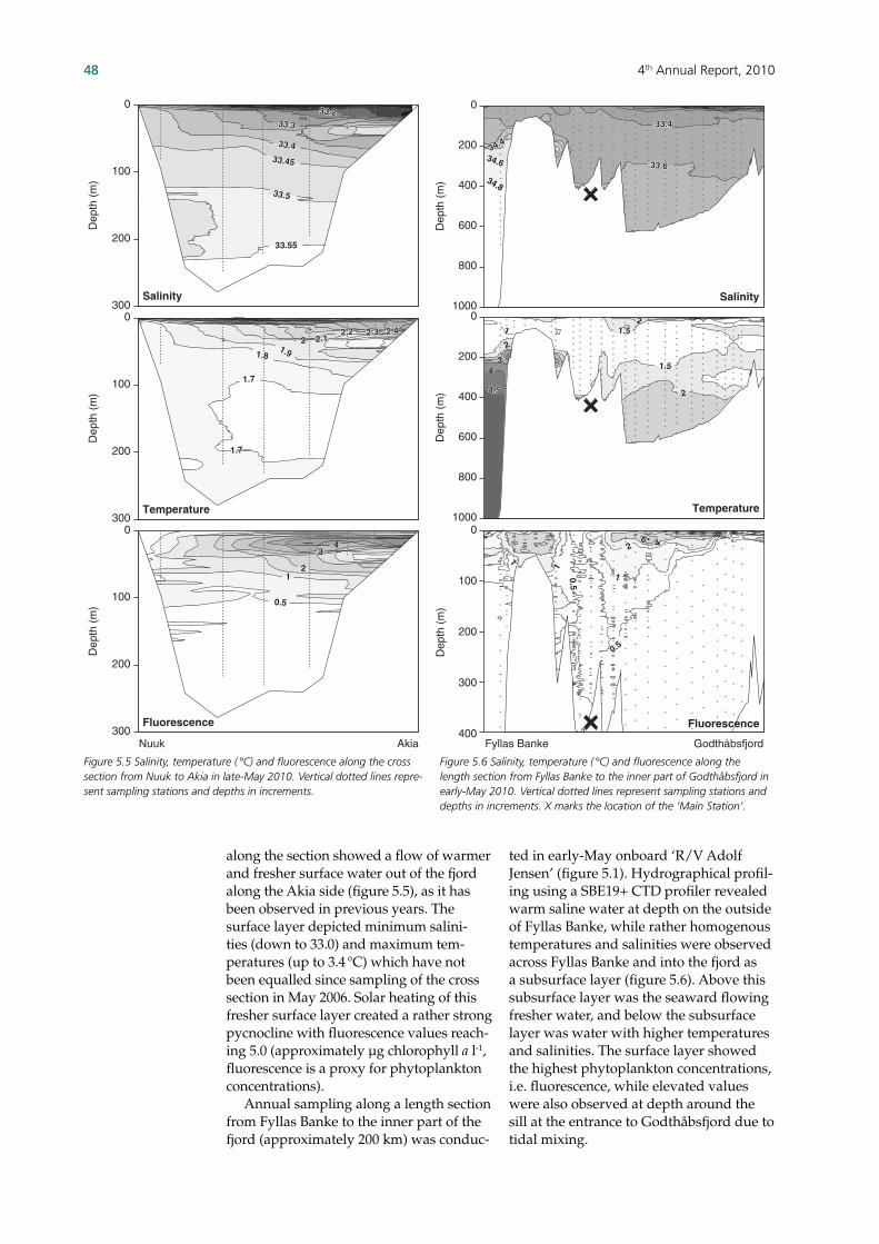
4th Annual Report, 201048
along the section showed a fl ow of warmer and fresher surface water out of the fjord along the Akia side (fi gure 5.5), as it has been observed in previous years. The surface layer depicted minimum salini-ties (down to 33.0) and maximum tem-peratures (up to 3.4 °C) which have not been equalled since sampling of the cross section in May 2006. Solar heating of this fresher surface layer created a rather strong pycnocline with fl uorescence values reach-ing 5.0 (approximately µg chlorophyll a l-1, fl uorescence is a proxy for phytoplankton concentrations). Annual sampling along a length section from Fyllas Banke to the inner part of the fjord (approximately 200 km) was conduc-
ted in early-May onboard ‘R/V Adolf Jensen’ (fi gure 5.1). Hydrographical profi l-ing using a SBE19+ CTD profi ler revealed warm saline water at depth on the outside of Fyllas Banke, while rather homogenous temperatures and salinities were observed across Fyllas Banke and into the fjord as a subsurface layer (fi gure 5.6). Above this subsurface layer was the seaward fl owing fresher water, and below the subsurface layer was water with higher temperatures and salinities. The surface layer showed the highest phytoplankton concentrations, i.e. fl uorescence, while elevated values were also observed at depth around the sill at the entrance to Godthåbsfjord due to tidal mixing.
Dep
th (
m)
Dep
th (
m)
Dep
th (
m)
33.333.3
33.233.2
33.433.4
33.4533.45
33.5533.55
33.533.5
1.91.91.81.8
2 2.12.12.22.2 2.32.3 2.42.4
1.71.7
1.71.7
34
21
0.50.5
300
200
100
0
300
200
100
0
300
200
100
0
AkiaNuuk
Salinity
Temperature
Fluorescence
33.3
33.2
33.4
33.45
33.55
33.5
1.91.8
2 2.12.2 2.3 2.4
1.7
1.7
34
21
0.5
Salinity
Temperature
Fluorescence
GodthåbsfjordFyllas Banke
Dep
th (
m)
Dep
th (
m)
Dep
th (
m)
33.633.6
33.433.4
34.434.4
34.634.6
34.834.8
1000
800
600
400
200
0
1000
800
600
400
200
0
1
1
0.50.5
0.50.5
1
2 46
2
1 1.51.5
1.51.5
2
2
34
4.54.5
33.6
33.4
34.4
34.6
34.8
1
1
0.5
0.5
1
2 46
2
1 1.5
1.5
2
2
34
4.5
400
300
200
100
0
Figure 5.5 Salinity, temperature ( °C) and fl uorescence along the cross section from Nuuk to Akia in late-May 2010. Vertical dotted lines repre-sent sampling stations and depths in increments.
Figure 5.6 Salinity, temperature ( °C) and fl uorescence along the length section from Fyllas Banke to the inner part of Godthåbsfjord in early-May 2010. Vertical dotted lines represent sampling stations and depths in increments. X marks the location of the ‘Main Station’.

4th Annual Report, 2010 49
Surface pCO2 along the length transect remained below the atmospheric concen-tration (i.e. 387 µatm, fi gure 5.7), except at two station near the entrance to the fjord where outgassing seemed to have occur-red. Decreasing values of pCO2 into the fjord, except at the innermost station(s), reached a minimum pCO2 of 103.1 µatm. Thus, the fjord appear to have been a stronger CO2 sink than in 2009, when higher pCO2 values were recorded at most stations in the fjord.
5.3 Pelagic sampling
Monthly sampling was conducted at the ‘Main Station’ (GF3, 64 °07’N 51 °53’W, fi g-ure 5.1) at the entrance to Godthåbsfjord. This sampling programme of abiotic and biotic parameters included vertical profi les of salinity, temperature, density, oxygen concentration, turbidity, irradiance (PAR) and fl uorescence using a SBE19+ CTD profi ler. Water samples were analyzed for concentrations of pigments (chlorophyll a and phaeopigments) and nutrients (NOx, PO4
3-, SiO4 and NH4+) at 1, 5, 10, 15, 20, 30,
50, 100, 150, 250 and 300 m. In addition, dissolved inorganic carbon and total al-kalinity were measured on water samples from 1, 5, 10, 20, 30 and 40 m, representing the euphotic zone. Particulate primary production mea-surements were conducted using short-term (approximately 2 h) free-drifting in situ C14 incubations corrected for in situ light conditions. The vertical sinking fl ux of material was measured using short-term (approximately 2 h) free-drifting par-ticle interceptor traps deployed at 65 m. We measured the total amount of particu-late material in the traps, and measured pigments (chlorophyll a and phaeopig-ments) and particulate carbon and nitro-gen in the collected material. The abun-dance and composition of phytoplankton and zooplankton was sampled using vertical hauls with 20 and 45 µm nets, re-spectively. Larger planktonic organisms, i.e. crabs, shrimps and fi sh larvae, were sampled by oblique hauls using a 335 µm bongo nets. This was also conducted along the length section in early-May.
Abiotic parametersHydrographical conditions at the ‘Main Station’ in the beginning of the year re-sembled conditions in previous years.
0 50 100 150 200 250Distance from FB4 (km)
Main station
pCO
2 (µ
atm
)
500
400
300
200
100
0
Salinity
Temperature
Irradiance
DecJan Mar May Jul Sep
Dep
th (
m)
Dep
th (
m)
Dep
th (
m)
300
200
100
0
300
200
100
0
100
75
50
25
0
33.5
34
33.5
32
29
330.
5
2
2
2
1
1
4
4
13
3
5 3
100
200
5075
25
10
5
Figure 5.7 pCO2 (µatm) in surface waters along the length section from Fyllas Banke (outermost station FB4, fi gure 5.1) to the inner part of Godthåbsfjord in early-May 2010. Horizontal dotted line represents atmospheric content (387 µatm).
Figure 5.8 Annual variation in salinity, temperature ( °C) and irradiance (PAR) at the ‘Main Station’ in 2010. Vertical dotted lines represent sampling days and depths in increments.

4th Annual Report, 201050
Winter, both early and late 2010, was characterised by a moderate stratifi ca-tion of the water column with warmer more saline water towards the bottom likely representing an infl ow of coastal water (salinities and temperatures up to 34.3 and 3.5 °C, respectively, fi gure 5.8). Vertical mixing of the water column fol-lowed during spring creating homogenous conditions throughout the entire water column with salinities just above 33 and temperatures below 1 °C. Solar heating of surface waters combined with outfl ow of melt water stratifi ed the water column during summer producing a surface layer with the lowest salinities (down to 18.5) and highest temperatures (up to 8.3) re-corded during the run of the programme. This pycnocline weakened during au-tumn, and only a moderate stratifi cation persisted during winter, as mentioned above. The light regime of the upper water column varied due to seasonal variations in incoming irradiance and absorption by suspended material in the water (e.g. phy-toplankton). Irradiance remained below 5 µmol photos m-2 s-1 at depths below 50 m, as it has been reported in previous years. The high pCO2 values reported in late 2009, i.e. above the atmospheric concen-tration, continued into January 2010 reaching a new maximum recorded value (734 µatm, fi gure 5.9). Afterwards values generally decreased until autumn, except for a peak in May. During autumn, surface pCO2 values reached a stable level well below the atmospheric concentration, which lasted for the rest of the year. Ave-rage recorded surface pCO2 in 2010 (297 µatm) signifi ed a decrease from the high 2009 average (340 µatm), while still re-maining above the levels in previous years (186-275 µatm from 2006 to 2008, respec-tively). Thus, it appears that the infl ow of CO2 rich coastal water persisted into early 2010, but during the rest of the year, Godthåbsfjord regained much of its CO2 uptake capacity. Infl ow of coastal water in early 2010 introduced high nutrient levels, particu-larly in deeper waters (maximum 12.3, 0.5 and 6.2 µM for nitrate/nitrite, phosphate and silicate, respectively, fi gure 5.10). High nutrient levels persisted throughout the water column until the onset of the phy-toplankton bloom in summer (July/Au-gust), although a moderate decrease was observed from May. The summer bloom resulted in depleted nutrient levels in the
Jun Dec Jun Dec Jun Dec Jun Dec Jun Dec Jun Dec2005 2006 2007 2008 2009 2010
pCO
2 (µ
atm
)
800
600
400
200
0
Figure 5.9 Annual variation in pCO2 (µatm) in the surface water at the ‘Main Station’ from late 2005 to 2010. Horizontal dotted line represents atmospheric content (387 µatm).
Figure 5.10 Annual variation in nitrate and nitrite (µM), phosphate (µM) and silicate (µM) concentrations at the ‘Main Station’ in 2010. Vertical dotted lines represent sam-pling days and depths.
Nitrate & nitriteNitrate & nitrite
PhosphatePhosphate
SilicateSilicate
DecJan Mar May Jul Sep
Dep
th (
m)
Dep
th (
m)
Dep
th (
m)
300
200
100
0
300
200
100
0
300
200
100
0
5
5
6
4
4
3
2
5
6
78
8
9
91010
1010
1212
1111
4
32
0.30.3
0.40.40.50.5
0.60.6
0.6
0.6 0.70.70.7
0.7
5
5
6
4
4
3
2
5
6
78
8
9
910
10
12
11
4
32
0.3
0.40.5
0.6
0.6 0.70.7
Nitrate & nitrite
Phosphate
Silicate

4th Annual Report, 2010 51
upper part of the water column (minimum of 0.06, 0.06 and 0.8 µM for nitrate/nitrite, phosphate and silicate, respectively). A break-down of the stratifi cation in autumn likely combined with benthic/pelagic re-mineralisation and introduction of nutrient rich coastal water resulted in re-established nutrient levels.
Biotic parametersThe phytoplankton biomass, i.e. chloro-phyll a concentrations, remained low du-ring winter months when light was limited (fi gure 5.11). Increased light conditions in spring brought on a phytoplankton bloom with increasing chlorophyll a concentra-tions. Vertical mixing at the ‘Main Station’ in spring resulted in elevated concentra-tions at depth. The following stratifi cation of the water column, due to freshwater
outfl ow and solar heating, maintained the bulk phytoplankton biomass within the euphotic zone (upper 50 m), resulting in peak pigment concentrations in July (chlorophyll a and phaeopigments 3.5 and 0.8 µg l-1, respectively). While the spring bloom in May was depicted in the primary production, the highest production value of 1382 mg C m-2 d-1 was recorded in July during the time of high surface tempera-ture and low salinity. This production val-ue is the second highest recorded since the programme was initiated in late 2005; the highest value was during May 2009 (1551 mg C m-2 d-1). Please note that previously reported seasonal primary production val-ues from 2009 (Juul-Pedersen et al. 2009) was underestimated due to an error in ir-radiance values used for light correction (also, annual values were presented as mg
Chlorophyll a
Phaeopigments
DecJan JanMar AprFeb May Jun Jul Aug Sep Oct Nov
Dep
th (
m)
Dep
th (
m)
Prim
ary
prod
uctio
n (m
g C
m–2
d–1
)
200
300
100
0
200
300
100
0
0.2
0.2
0.40.6
0.5
0.3
0.3
0.10.1
0.3
0.5
0.6
0.60.8
0.7
0.4
11
2
0.1
0.1
0.2
0.20.4
800
1600
1200
400
0
Figure 5.11 Annual varia-tion in chlorophyll a con-centration (µg l-1), phaeo-pigments concentration (µg l-1) and primary production (mg C m-2 d-1) at the ‘Main Station’ in 2010. Vertical dotted lines on chlorophyll a and phaeopigments plots represent sampling days and depths.

4th Annual Report, 201052
C m-2 y-1 while they should have been in g C m-2 y-1). Hence, the annual integrated pri-mary production in 2010 (106 g C m-2 y-1) was the highest recorded during the run of the programme (76.0, 104, 91.1 and 99.7 g C m-2 y-1 in 2006, 2007, 2008 and 2009, respectively).
The plankton communityVertical net hauls (20 µm) from 0-60 m was used to sample for phytoplankton species composition. The phytoplankton commu-nity showed the characteristic pattern with diatoms dominating throughout the year, except during the spring bloom when
Phaeocystis sp. (Haptophyceae) was the major constituent (fi gure 5.12). Only 2009 differed from this general seasonal species succession, as Phaeocystis sp. remained absent all through the year. In contrast, the higher percent contributions of dinofl a-gellates and other phytoplankton species during mid-winter in 2010 are consistent with 2009. Overall, more than half of the phytoplankton community integrated over 2010 consisted of the three algae groups Chaetoceros spp., Phaeocystis sp. and Thalassiosira spp. (table 5.1), as it was ob-served prior to 2009 (i.e. 2006-08). Vertical zooplankton net hauls (45 µm WP2 net) were conducted from 0-100 m. The copepod abundance peaked about a month earlier than in previous years (47000 individuals m-3 during July, fi gure 5.13), but with a peak value comparable to previous years (19000-70000 individu-als m-3 during 2006-2009). In contrast, the peak copepod nauplii abundance in July (117995 individuals m-3) was by far the highest concentration recorded during the fi ve years of sampling (28000-63000 indi-viduals m-3 during 2006-2009), possibly linked to high temperatures. While previ-ous years showed a month separation between the peak in nauplii and copepods there was no separation between the two groups in 2010. The copepod community was again in 2010 dominated by Microsetella sp., except
J F M A M J J A S O N D
Com
posi
tion
(%)
0
20
40
60
80
100 Diatoms
Dinoflagellates
Silicoflagellates
Haptophyceae
Others
Month
Figure 5.12 Seasonal variation in phytoplankton community composition (%) at the ‘Main Station’ during 2010.
2006 2007 2008* 2009 2010
Chaetoceroswighamii
30.5 Chaetoceros spp. (ex debilis)
20.1 Thalassiosira spp. 27.9 Chaetoceros spp. 42.4 Chaetoceros spp. 37.2
Phaeocystis sp. 45.5 Phaeocystis sp. 36.3 Phaeocystis sp. 50.4 Thalassiosira spp. 58.4 Phaeocystis sp. 51.0
Thalassiosira antarctica
53 Thalassiosira spp. 52.3 Chaetoceros spp. 62.1 Pauliella taeniata 66.8 Thalassiosira spp. 61.4
Thalassionema nitzschioides
58.1 Chaetoceros debilis
65.5 Fragilariopsis spp. 70.0 Fragilariopsis spp. 71.0 Centric diatoms undet.
66.8
Dictyocha speculum
62.7 Thalassionema nitzschioides
78.6 Navicula spp. 73.9 Dinobryon baltica 74.4 Protoperidinium spp. 70.8
Pseudonitzschia cf seriata
66.2 Fragilariopsis oceanica
82.2 Protoperidinium spp. 77.5 Centric diatoms undet.
77.6 Leptocylindrus danicus
72.8
Thalassiosira nordenskioeldii
69.1 Dictyocha speculum
83.6 Pseudonitzschia spp. 80.5 Protoperidinium spp. 80.2 Stenosomella spp. 74.6
Nitzschia frigida 71.7 Aulacoseira sp. 84.9 Podosira spp. 83.2 Dictyocha speculum 82.4 Alexandrium sp. 76.1
Dinobrion balticum
74 Cocconeis spp. 86.1 Leptocylindrus spp. 85.7 Leptocylindrus danicus
83.8 Skeletonema sp. 77.6
Thalassiosira bioculata
76.1 Ceratulina sp. 87.0 Peridenella catenata 87.6 Navicula spp. 85.2 Dictyocha speculum 78.9
*From January to August
Table 5.1 Ten most dominant phytoplankton species integrated over the year as their relative accumulated proportion of total cell counts (%) at the 'Main Station' in 2006-2010.

4th Annual Report, 2010 53
during February when Microcalanus com-prised more (45.5 vs. 39.4 %, respectively; fi gure 5.13). The only other species con-tributing signifi cantly to the copepod com-position was Oithona spp. (up to 22.6 %) and Pseudocalanus spp. (up to 17 %), while Calanus spp. only contributed up to 8.5 % of the total copepod abundance. Similar to previous years, Calanus spp. was mainly present during the spring bloom in May. However, it is important to keep in mind that the specifi c species contribution to the copepod community biomass will differ from the abundance, as signifi cant size dif-ferences occur between these species. The peak abundance of other zooplank-ton (36729 individuals m-3) coincided with the maximum copepod abundance in July. While the seasonal succession observed for Bivalvia larvae (i.e. spring) and Gas-tropoda larvae and rotifera (i.e. summer) resembled previous years, Bivalvia larvae peaked later (i.e. summer) than generally observed. Moreover, foraminifera were almost absent throughout the year. To as sess shellfi sh as well as fi sh lar-vae at the ‘Main Station’ (GF3), single oblique sampling with a bongo net (335 µm) was used each month during 2008 (except June), 2009 (except October) and 2010. Additional samplings with a double oblique bongo net (335 and 500 µm) were conducted along a length section from offshore Fyllas Banke to the inner part of the fjord during May 2006-2010. Thirteen stations were sampled in May 2006, four stations in 2007 and 2008, three stations in 2009 and fi ve stations in 2010. At the ‘Main Station’ (GF3), the highest concentration of fi sh larvae were usually found in spring (March-May, 2006-2008). In 2009 and 2010, however, the highest concentration was found in summer (July; fi gure 5.14A). This was caused by a decrease in abundance of sand eel (Ammo-dytes sp.) larvae in spring and an increase in the abundance of capelin (Mallotus villo-sus) larvae in summer in the 2009 and 2010 samples. Overall, the total abundance of fi sh larvae (individuals 100 m-3) has declined since the beginning of the programme in 2006. This is caused by gradually declining sand eel larvae abundance. In March 2006, 14.7 individuals 100 m-3 were caught in the samples, whereas in March 2010 only 0.003 individuals 100 m-3 were caught. In 2006-2008 sand eel larvae was the dominating species in spring at the main
station, whereas in 2009 arctic shanny (Stichaeus punctatus) was the dominating species. However, in 2010 sand eel larvae was again the dominating species during spring at the ‘Main station’ (fi gure 5.14B), but at the lowest abundance (individuals m-3) since 2006. A temporal shift in species composi-tion occurs during summer at the ‘Main Station’. In 2009 and 2010, sand eel was the dominating species in spring whereas capelin was dominating in late summer/early fall (fi gure 5.14B). Cod larvae (Gadus morhua) were found in May, June and July and were the dominating species in June. In May, the length section in the fjord shows the same pattern in fi sh larvae concentrations and species composition as previous years. Highest concentrations were found closer to the head of the fjord at
Others
Microsetella sp.
Calanus spp.
Pseudocalanus
Oncaea
Oithona spp.
Acartia spp.
Microcalanus
Metridia spp.
Indi
vidu
als
(m–3
)C
ompo
sitio
n (%
)In
divi
dual
s (m
–3)
25000
0
50000
75000
100000
125000
150000
175000
10000
0
20000
30000
40000
50000
60
0
20
40
80
100
J F M A M J J A S O N D2010
A
B
C
Copepods
Nauplii
Other zoo plankton
Figure 5.13 Annual varia-tion in abundance (indi-viduals m-3) of copepod nauplii and copepods (i.e. copepodites and adult stages) (A), copepod com-munity composition (%) (B) and abundance of other zooplankton groups (individuals m-3) (C) at the ‘Main Station’ in 2010. Er-ror bars represent standard deviation.

4th Annual Report, 201054
the ‘Main Station’ (fi gure 5.15A), although lower than previous years due to decreased abundance of sand eel larvae. Species com-position also varied on the length section
with fewer species in the samples deeper inside the fjord (fi gure 5.15B). Cod larvae were found both close to the inlet and in the middle part of the fjord.
0
0.02
0.04
0.06
0.08
0.10
0.12
Others
Pholis fasciatus
Myoxocephalusscorpius
Liparis gibbus
Lumpenuslampretaeformis
Leptagonus decagonus
Gadus ogac
Hippoglossoidesplatessoides
Mallotus villosus
Ammodytes sp.
Leptochlinusmaculatus
Stichaeus punctatus
Gadus morhua
Indi
vidu
als
(100
m–3
)S
peci
es c
ompo
sitio
n (%
)
60
0
20
40
80
100
Jan Feb Mar Apr May Jun Jul Aug Sep Oct Nov Dec
2010
A
B
0
0.01
0.02
0.03
0.04
Others
Pholis fasciatus
Liparis gibbus
Leptagonus decagonus
Hippoglossoidesplatessoides
Bathylagus euryops
Ammodytes sp.
Leptochlinus maculatus
Stichaeus punctatus
Gadus morhua
Indi
vidu
als
(100
m–3
)S
peci
es c
ompo
sitio
n (%
)
60
0
20
40
80
100
A
B
FB
4
FB
3.5
FB
3
FB
2.5
FB
2
FB
1.5
FB
1
GF
1
GF
2
GF
3
GF
4
GF
5
GF
6
GF
7
GF
8
GF
9
GF
10
Station
Figure 5.14 Annual vari-ation in abundance (indi-viduals 100 m-3) (A) and community composition (%) (B) of fi sh larvae at the ‘Main Station’ in 2010.
Figure 5.15 Variation in abundance (individuals 100 m-3) (A), and commu-nity composition (%) (B) of fi sh larvae on the length section in May 2010.

4th Annual Report, 2010 55
Fish larvae species composition seems to vary between years with most species found in 2008 and 2010 (table 5.2). At the ‘Main Station’ (GF3), seasonal patterns in the abundance of shellfi sh (Chionoecetes opilio, Hyas sp., Pandalus sp.) show similarities over the past three years (fi gure 5.16). All three species of deca-pods were present in samples from April to August. Abundance of Chionoecetes opilio (snow crab) and Hyas sp. (sand crab) peaked in May, respectively, in 2009 and 2010, whereas Pandalus sp. (shrimp) peaked in June 2010, i.e. one month de-layed compared to the two previous years. Density of Hyas sp. and Pandalus sp. exceeded previous values from 2008 and 2009 almost twofold. Larvae stage zoae I of C. opilio and Hyas sp. dominated samp-les from April to June, whereas larvae stage zoae II were more abundant in July.
Low concentrations of megalope stage of C. opilio and Hyas sp. were observed in Oc-tober. Throughout the time series, abun-dance of C. opilio has been low compared to Hyas sp. and Pandalus sp. Community composition at the ‘Main Station’ (GF3) varies between years. In 2009, the ratio of Sagitta sp. (arrow worm) was relative higher from May to July com-pared with 2008 and 2010 (fi gure 5.17) and Sagitta sp. remained the single most abun-dant species, except for February, April and June. Another consistently abundant species was Ctenophora sp. (comb jelly), comprising 40 % in September. In con-trast, jellyfi sh dominated samples in 2010 from January to March, while Ctenophores dominated in July and from September and onwards. Sagitta sp. was recorded in considerably lower numbers than during the previous years.
20112008 2009 2010 20112008 2009 2010Year
Indi
vidu
als
m-3
Chionoecetes opilio
Hyas sp.
Pandalus sp.
Sagitta sp.
Ctenophora sp.
Other jellyfish
0.8
0.6
0.4
0.2
00.8
0.6
0.4
0.2
00.8
0.6
0.4
0.2
0
Figure 5.16 Annual varia-tion in abundance of Chionoecetes opilio, Hyas sp., Pandalus sp., Sagitta sp., Ctenophora sp. and other jellyfi sh from 2008 to 2010 at the ‘Main Station’ (GF3). Samples were col-lected each month except November 2008 and August 2009.

4th Annual Report, 201056
Along the length transect from Fyllas Banke (offshore) to the inner part of the fjord (GF10) highest concentrations of
sand crab larvae (Hyas sp.) were recorded at the offshore station FB2.5 in 2006 and 2010 (fi gure 5.18). Both crab and shrimp larvae are to be found at almost all stations along the length transect, with variations in density among species and between stations. Highest numbers of individuals (individuals m-3) were observed in 2006 followed by a sharp decline in 2007 to 2009. Nevertheless, crab and shrimp lar-vae increased signifi cantly in 2010. Along the length transect, the community composition differed not only between sta-tions but also between years (fi gure 5.19). At station GF10, located in the inner part of the fjord, larvae of Ctenophores, jellyfi sh and Sagitta sp. dominated the samples in 2009, whereas Ctenophora sp. were absent in 2010 which instead was dominated by Sagitta sp. with occurrence of shrimp and crab (Hyas sp.) larvae. Sagitta sp. dominated at GF3 (‘Main Station’) in 2009, but was negligible at GF3 and only recorded in a low numbers at GF7 in 2010. The abundance of Pandalus sp. and Hyas sp. were considerably higher in 2010 compared to previous years. At the outer fjord, larvae of C. opilio and especially Hyas spp. were more abundant than shrimp larvae, and Hyas spp. was dominant at the shallower parts of the bank.
Table 5.2 Species list of fi sh larvae 2006-2010.
Species list 2006 2007 2008 2009 2010
Gadus morhua × × × × ×
Stichaeus punctatus × × × × ×
Leptochlinus maculatus × × × × ×
Ammodytes sp. × × × × ×
Mallotus villosus × × × ×
Aspidophoroides monopterygius × × ×
Bathylagus euryops × × × ×
Cyclothone sp. ×
Liparis sp. ×
Liparis gibbus ×
Pholis sp. × × ×
Pholis fasciatus ×
Reinhardtius hippoglossoides × ×
Myoxocephalus scorpius × ×
Hippoglossoides platessoides × × ×
Sebastes sp. ×
Gadus ogac × × ×
Leptagonus decagonus × ×
Agonidae ×
Lumpenus lampretaeformis × ×
Total 7 10 13 11 13
Chionoecetes opilio
Hyas sp.
Pandalus sp.
Sagitta sp.
Ctenophora sp.
Other jelly fish
J F M A M J J A S O N D
2010
Per
cent
(%
)
0
20
40
60
80
100
0
20
40
60
80
100
Figure 5.17 Annual variation in community composition (%) in 2009 (upper) and 2010 (lower) at the ‘Main Station’ (GF3). Samples were col-lected each month except August 2009.

4th Annual Report, 2010 57
Vertical sinking fl ux
Vertical sinking fl ux of particulate material was measured using monthly deployments of free-drifting short-term (approximately 2 h) sediment traps collecting material sinking from the euphotic zone (deployed at 65 m). Low sinking fl uxes of both total particulate carbon (TPC) and chlorophyll a (Chl a) were observed in winter and spring, i.e. until April, when an increase occurred during the developing spring phytoplank-ton production (fi gure 5.20). The peak Chl a sinking fl ux (7.4 mg m-2 d-1) in May cor-responds with the rather moderate spring bloom previously described, while Chl a fl uxes related to the higher summer bloom may have been missed due to the lack of data from August. The C:N ratio of the ma-terial collected during spring and summer
(between 7.4 and 8.4 mol:mol from May to August) also indicates a strong phytoplank-ton based carbon component, i.e. close to the Redfi eld ratio (6:6 mol:mol) typical of fresh algal cells. This is further supported by the δ13C and δ15N values during this productive period. Variable Chl a sink-ing fl uxes during spring and summer are contrasted by a moderate decrease in TPC sinking fl uxes. The abrupt decline in δ13C values during September was likely caused by a higher input of terrestrial material du-ring discharge and seaward export of melt water. The annually integrated TPC sinking fl ux (351.2 g C m-2 y-1) was comparable to previously reported values (between 253.9 and 431.5 g C m-2 y-1 from 2006-09). Sinking fl uxes of total material (data not presented) may likely have been overestimated in
Chionoecetes opilio
Hyas sp.
Pandalus sp.
6
5
4
3
2
1
02.0
1.5
1.0
0.5
02.0
1.5
1.0
0.5
0
Indi
vidu
als
m-3
2008
2007
2006
2010
2009
FB
4F
B3.
5F
B3
FB
2.5
FB
2F
B1.
5F
B1
GF
1G
F2
GF
3G
F4
GF
5G
F6
GF
7G
F8
GF
9G
F10
FB
4F
B3.
5F
B3
FB
2.5
FB
2F
B1.
5F
B1
GF
1G
F2
GF
3G
F4
GF
5G
F6
GF
7G
F8
GF
9G
F10
Station Station
Figure 5.18 Annually vari-ation in abundance (indi-viduals m-3) of crab and shrimp larvae along the length section from Fyllas Banke (offshore) to the in-ner part of Godthåbsfjord conducted in May 2006 to 2010. In 2009, no samp-ling was carried out at Fyllas Banke.
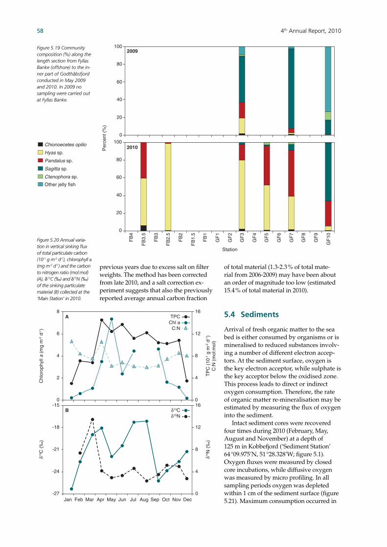
4th Annual Report, 201058
previous years due to excess salt on fi lter weights. The method has been corrected from late 2010, and a salt correction ex-periment suggests that also the previously reported average annual carbon fraction
of total material (1.3-2.3 % of total mate-rial from 2006-2009) may have been about an order of magnitude too low (estimated 15.4 % of total material in 2010).
5.4 Sediments
Arrival of fresh organic matter to the sea bed is either consumed by organisms or is mineralised to reduced substances involv-ing a number of different electron accep-tors. At the sediment surface, oxygen is the key electron acceptor, while sulphate is the key acceptor below the oxidised zone. This process leads to direct or indirect oxygen consumption. Therefore, the rate of organic matter re-mineralisation may be estimated by measuring the fl ux of oxygen into the sediment. Intact sediment cores were recovered four times during 2010 (February, May, August and November) at a depth of 125 m in Kobbefjord (‘Sediment Station’ 64 °09.975’N, 51 °28.328’W; fi gure 5.1). Oxygen fl uxes were measured by closed core incubations, while diffusive oxygen was measured by micro profi ling. In all sampling periods oxygen was depleted within 1 cm of the sediment surface (fi gure 5.21). Maximum consumption occurred in
Chionoecetes opilio
Hyas sp.
Pandalus sp.
Sagitta sp.
Ctenophora sp.
Other jelly fish
FB
4
FB
3.5
FB
3
FB
2.5
FB
2
FB
1.5
FB
1
GF
1
GF
2
GF
3
GF
4
GF
5
GF
6
GF
7
GF
8
GF
9
GF
10
Station
60
0
20
40
80
100
2009
2010Per
cent
(%
)
0
20
40
60
80
100Figure 5.19 Community composition (%) along the length section from Fyllas Banke (offshore) to the in-ner part of Godthåbsfjord conducted in May 2009 and 2010. In 2009 no sampling were carried out at Fyllas Banke.
DecJan Feb Mar Apr May Jun Jul Aug Sep Oct Nov
16
12
8
4
0
8
6
4
2
0
TPCChl a
C:N
δ13Cδ15N
-15
-18
-21
-24
-27
16
12
8
4
0
Chl
orop
hyll
a (m
g m
-2 d
-1)
δ13C
(‰
)
TP
C (
10-1 g
m-2 d
-1)
C:N
(m
ol:m
ol)
δ15N
(‰
)
A
B
Figure 5.20 Annual varia-tion in vertical sinking fl ux of total particulate carbon (10-1 g m-2 d-1), chlorophyll a (mg m-2 d-1) and the carbon to nitrogen ratio (mol:mol) (A), δ13C (‰) and δ15N (‰) of the sinking particulate material (B) collected at the ‘Main Station’ in 2010.

4th Annual Report, 2010 59
August, just after the summer bloom when sinking fl uxes of algal material most likely was high (Chl a sinking fl ux from August is missing). Return of dissolved inorganic carbon (DIC) to the water column remained rather constant throughout the year (table 5.3). Oxygen consumption rates were high-est during summer and autumn/winter (> 1 µmol cm-3 d-1 in August and Novem-ber) compared to winter/spring (< 1 µmol cm-3 d-1 in February and May). Overall, seasonal differences seem to indicate high-est benthic activity in summer and autumn, possibly due to the high organic input and elevated temperatures observed also at depth, which is in contrast to previous years with more acti-vity in spring.
5.5 Benthic fauna and fl ora
Benthic fauna
The fauna found on the bottom of Green-land fjords are important components of the marine food web. On average they are estimated to consume approximately 20 % of the primary production (Blicher et al. 2009). Benthic fauna are also the preferred prey for predators such as walruses and eiders (Born et al. 2003, Merkel et al. 2007). Moreover, specifi c species such as sea ur-chins may actively infl uence the structure of the ecosystem through intense grazing of macro algae and subsequent formation of ‘sea urchin barrens’. Finally, the benthic community consists of very high species richness with frequent observation of more than 100 species m-2 in outer part of fjords (Sejr et al. 2010). In Kobbefjord, the sea urchin Strongy-locentrotus droebachiensis and the scallop Chlamys islandica are found in large quanti-ties in the shallow parts of the fjord (10-75 m) where they constitute the majority of the biomass (Blicher et al. 2009). Annual shell growth rates have been determined for both species. Additionally, a seasonal study looking at the growth dynamics of the different soft tissues of C. islandica produced a growth model indicating a negative infl uence of temperature (Blicher et al. 2010). Thus, a future warming of the upper water column can be expected to increase the metabolic cost with potential negative effects on the energy available for growth and reproduction. Since 2007, the energetic status of the two species has been surveyed in May at a
O2 (µM)
O2 consumption (µmol cm–3 d–1)
Dep
th (
cm)
Dep
th (
cm)
1.0
0.6
0.8
0.4
0.2
0
–0.2
–0.4
1.0
0.6
0.8
0.4
0.2
0
–0.2
–0.4
0 100 200 300 400
0 0.5 1.0 1.5
0 1 2 3 4 5
0 0.5 1.0 1.5
0 0.5 1.0 1.5
0 100 200 300 400
0 100 200 300 400 0 100 200 300 400
February May
August November
Figure 5.21 Vertical concentration profi les of oxygen (closed dots) and modelled con-sumption rates (solid line) from micro electrode profi les with sediment depth for each of the four sampling periods. Error bars represent standard error of the mean.
Table 5.3 Sediment-water exchange rates of O2 (TOU), NO3- + NO2
-, PO43- and SiO4
measured in intact sediment cores, diffusive oxygen uptake by the sediment (DOU) and the ratios of DOU to TOU. n denotes the number of sediment cores. Positive values for NO3 + NO2
-, PO43- and SiO4 represent a release from the sediment to the water column,
while positive values for TOU and DOU represent an uptake into the sediment. All rates are in mmol m-2 d-1. SE denotes the standard error of the mean.
Month
Parameter February May August November n
TOU 8.89 ±1.35 6.32 ±0.89 4.06 ±1.03 5.73 ±1.93 6
DOU 4.40 – 4.60 – 12.40 – 5.42 – 3
TOU/DOU 2.02 – 1.37 – – – 1.06 – –
DIC 4.39 ±0.70 5.70 ±0.83 4.75 ±1.20 4.35 ±32 6
PO43- 0.08 ±0.16 0.12 ±0.01 –0.25 ±0.05 – – 6
NO3- + NO2
- 0.17 ±0.04 0.25 ±0.04 – – – – 6
SiO4 1.03 ±0.17 1.11 ±0.16 4.30 ±0.89 1.79 ±0.50 6
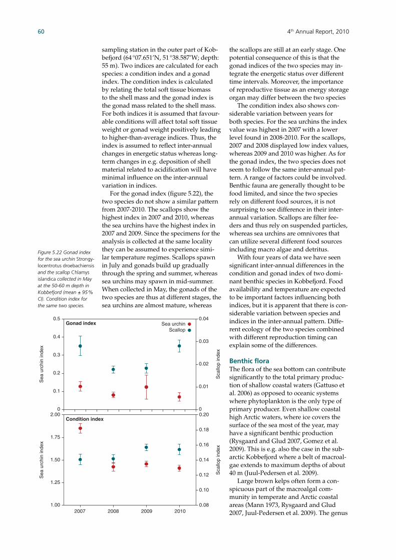
4th Annual Report, 201060
sampling station in the outer part of Kob-befjord (64 °07.651’N, 51 °38.587’W; depth: 55 m). Two indices are calculated for each species: a condition index and a gonad index. The condition index is calculated by relating the total soft tissue biomass to the shell mass and the gonad index is the gonad mass related to the shell mass. For both indices it is assumed that favour-able conditions will affect total soft tissue weight or gonad weight positively leading to higher-than-average indices. Thus, the index is assumed to refl ect inter-annual changes in energetic status whereas long-term changes in e.g. deposition of shell material related to acidifi cation will have minimal infl uence on the inter-annual variation in indices. For the gonad index (fi gure 5.22), the two species do not show a similar pattern from 2007-2010. The scallops show the highest index in 2007 and 2010, whereas the sea urchins have the highest index in 2007 and 2009. Since the specimens for the analysis is collected at the same locality they can be assumed to experience simi-lar temperature regimes. Scallops spawn in July and gonads build up gradually through the spring and summer, whereas sea urchins may spawn in mid-summer. When collected in May, the gonads of the two species are thus at different stages, the sea urchins are almost mature, whereas
the scallops are still at an early stage. One potential consequence of this is that the gonad indices of the two species may in-tegrate the energetic status over different time intervals. Moreover, the importance of reproductive tissue as an energy storage organ may differ between the two species The condition index also shows con-siderable variation between years for both species. For the sea urchins the index value was highest in 2007 with a lower level found in 2008-2010. For the scallops, 2007 and 2008 displayed low index values, whereas 2009 and 2010 was higher. As for the gonad index, the two species does not seem to follow the same inter-annual pat-tern. A range of factors could be involved. Benthic fauna are generally thought to be food limited, and since the two species rely on different food sources, it is not surprising to see difference in their inter-annual variation. Scallops are fi lter fee-ders and thus rely on suspended particles, whereas sea urchins are omnivores that can utilize several different food sources including macro algae and detritus. With four years of data we have seen signifi cant inter-annual differences in the condition and gonad index of two domi-nant benthic species in Kobbefjord. Food availability and temperature are expected to be important factors infl uencing both indices, but it is apparent that there is con-siderable variation between species and indices in the inter-annual pattern. Diffe-rent ecology of the two species combined with different reproduction timing can explain some of the differences.
Benthic fl oraThe fl ora of the sea bottom can contribute signifi cantly to the total primary produc-tion of shallow coastal waters (Gattuso et al. 2006) as opposed to oceanic systems where phytoplankton is the only type of primary producer. Even shallow coastal high Arctic waters, where ice covers the surface of the sea most of the year, may have a signifi cant benthic production (Rysgaard and Glud 2007, Gomez et al. 2009). This is e.g. also the case in the sub-arctic Kobbefjord where a belt of macroal-gae extends to maximum depths of about 40 m (Juul-Pedersen et al. 2009). Large brown kelps often form a con-spicuous part of the macroalgal com-munity in temperate and Arctic coastal areas (Mann 1973, Rysgaard and Glud 2007, Juul-Pedersen et al. 2009). The genus 2007 2008 2009 2010
0.04
0.03
0.02
0.01
0
0.5
0.4
0.3
0.2
0.1
0
Sea urchinScallop
Gonad index
Condition index2.00
1.75
1.50
1.25
1.00
0.20
0.14
0.16
0.18
0.12
0.10
0.08
Sea
urc
hin
inde
xS
ea u
rchi
n in
dex
Sca
llop
inde
xS
callo
p in
dex
Figure 5.22 Gonad index for the sea urchin Strongy-locentrotus droebachiensis and the scallop Chlamys islandica collected in May at the 50-60 m depth in Kobbefjord (mean ± 95 % CI). Condition index for the same two species.

4th Annual Report, 2010 61
Laminaria and related species produce an annual blade, the size of which refl ects growth conditions of the preceding year with respect to e.g. light availability and thus sea ice cover. The size of the annual blade is therefore selected as a monitoring variable. In higher latitudes the annual growth of sugar tangle, Saccharina latis-sima, can be estimated based on a single sampling in late summer, since the new blade is separated by clear constrictions from the old blade, which may remain for 1-2 years (Lund 1951, Dunton 1985, Bo-rum et al. 2002). At lower latitudes like in Nuuk the blades are turned over at faster rates, however, and the tip may be worn off before the annual growth is completed. Laminaria longicruris shares many morpho-logical characteristics with S. latissima, and also produces a new blade each year, but does not seem to form as clear constric-tions between years as do S. latissima. In Kobbefjord, L. longicruris is a domi-nant kelp, while S. latissima has not been recorded. The programme therefore uses the size of the annual blade of L. longicru-ris as a monitoring variable. Because of fast growth rates and wearing off at the tips, the new blades are typically long but lack their extremity by the end of summer, and blade size therefore refl ects a mini-mum estimate of annual growth (Juul-Pedersen et al. 2009).
L. longicruris was collected by diver at 5-6 m depth in the outer, southern part of Kobbefjord on 17 August 2010. A total of 18 mature specimens having blades longer than 1.5 m was collected at a protected site where sea ice is expected to form in winter (64 °08.408’N; 51 °35.158’W) and 17 speci-mens were collected at an exposed site with less sea ice (64 °07.782’N; 51 °37.113’W). As Laminaria was grazed down by sea urchin at the usual exposed sampling site, we sampled a few hundred meters closer to the mouth of the fjord compared to 2007-2009. At the original sampling site, remains of some stems and blades were still being grazed and thereby evidenced the cause of the loss of the population. The size of the blades did not show any consistent difference between the protected and the exposed site over the monitoring period 2007-2010 (fi gure 5.23; left panel), even though the sites likely experienced differences in sea ice cover. Apparently, Kobbefjord was moderately covered by sea ice during the winter 2007/2008, markedly covered in the win-ter 2008/2009 (3-4.5 months in 2007/2008 and 5.5 months in 2008/2009, Hansen et al. 2010) but only slightly covered during the winter 2009/2010 (satellite images indicate that the fjord was free of ice all winter: http://ocean.dmi.dk/arctic/nuuk.php). In particular, during 2009, algae at
Bla
de le
ngth
(cm
)
Exposed
Protected
0
100
200
300
0
50
100
150
200
250
2007 2008 2009 20102007 2008 2009 2010
Bla
de b
iom
ass
(g d
w)
N c
onte
nt (
% o
f dw
)
0
0.5
1.0
1.5
2.0
0
20
40
60
80
C/N
(m
ol/m
ol)
A
B
C
D
Figure 5.23 Length (A), biomass (B), nitrogen content (C) and C/N ratio (D) of blades of mature Laminaria longicruris with blade lengths larger than 1.5 m collected at a protected and an exposed site in Kobbefjord in Sep-tember 2007 and August 2008-2010.

4th Annual Report, 201062
the protected site were likely to have ex-perienced a longer ice covered period and thus to have received less incoming light than those at the protected site, but there was no difference in growth rate between the two sites. However, the annual growth of Laminaria in Kobbefjord is large relati-ve to that in Young Sund, NE Greenland where sea ice covers the fjord 9-10 months of the year (Borum et al. 2002). The average length of the blades was relatively similar between years as well, varying from a minimum of 188 cm at the exposed site in 2007 to a maximum of 227 cm at the same site in 2010 (fi gure 5.23; left panel). The biomass of the blades varied more between years, showing a minimum of 120 g dw at the protected site in 2007 and a maximum of 192 g dw at the exposed site in 2010. The generally low values recorded in 2007 could be related to the later sampling that year (September) than the following years (August), resul-ting in a larger risk of blade erosion by autumn storms. Nitrogen and carbon content also did not show any consistent differences between the two sites. In most years, N-le-vels and C/N-levels at the two sites were relatively similar, only 2007 showed a marked dif-ference with an extremely low N-content and an extremely high C/N-ratio at the protected site. Overall N-levels varied with a factor of about 2 from a minimum of 0.67 % at the protected site in 2007 to a maximum of 1.38 % at the same site in 2008 (fi gure 5.23; right panel). The C/N levels ranged from a minimum of 26 at the exposed site in 2008 to a maximum of 67 at the protected site in 2007 (fi gure 5.23; right panel).
The nitrogen content refl ects the balan-ce between demand and supply. In winter, when the supply of inorganic nutrients is relatively high and the demand low, ni-trogen reserves build up, and are drained during the following summer when the demand is high and the supply low. Re-lease of spores may exert an extra drain on the N reserves in late summer. Nitrogen concentrations are therefore likely to reach a minimum by the end of summer. Carbon concentrations, by contrast, are likely to be highest in late summer, as carbohydrates have been built up by photosynthesis over the summer. These mechanisms may explain the generally lower N content and higher C/N-ratio in the September sampling of 2007 relative to the August samplings of 2008-2010. The differences in levels of nitrogen content and C/N ratio between August samplings of 2008-2010 must refl ect additional year-to-year varia-tion in supply and demand of N and car-bon storage (fi gure 5.23; right panel). With four years of data, the last three representing August, we see that the blades of the kelp vary around a mean length of about 2.1 m, a biomass of about 176 g dw, a nitrogen content of about 1.2 % dw and a C/N ratio of about 33 at the two sites (mean of the last three years of data). As the blades apparently do not refl ect the expected differences in sea ice cover be-tween sites nor between years, quite large variations in growth conditions are likely needed to identify a signifi cant change in blade size of Laminaria longicruris.
5.6 Seabirds
Two major seabird colonies near Nuuk are included in the MarineBasis programme. Additional seabird colonies in the Nuuk area have been visited since 2007. Among them, the kittiwake (Rissa tridactyla) colonies of the Godthåbsfjord (fi ve in total) were sur-veyed and the results are included in this report. The seabird counts from MarineBa-sis are reported annually to the Greenland Seabird Colony Database maintained by the National Environmental Research In-stitute (http://www.dmu.dk/Greenland/Olie+og+Miljoe/Havfuglekolonier).
Qeqertannguit (colony code: 64035) Qeqertannguit in the inner part of Godt-håbsfjord (fi gure 5.1) is a low-lying is-land that holds the largest diversity of
Kittiwake (Rissa tridactyla). Photo: Carsten Egevang.

4th Annual Report, 2010 63
breeding seabirds in the Nuuk District. Especially surface feeders such as gulls (Laridae) and arctic tern (Sterna paradisaea) are well represented at the site (table 5.4). Counts of the entire island were conduct-ed 3 June (early in the incubating period) using direct counts of Apparently Occu-pied Nests (AON) or territorial behaviour as a criterion of breeding pairs. The steep cliff in the middle of the southeast facing side of the island (kittiwake and Iceland gull (Larus glaucoides)) and a smaller cliff on the north facing side (Iceland gull) were counted from the sea side, using a boat as platform while all other counts were conducted on land. Other birds observed 3 June (not con-sidered breeding or not systematically censured) included one long-tailed duck (Clangula hyemalis), several snow buntings (Plectrophenax nivialis) and one Red-breast-ed merganser (Mergus serrator). Black-headed gull (Chroicocephalus ridibundus) was observed on the island 17 May. The arctic tern colony appeared not to have active breeders 3 June, when 54 birds were observed. On 17 May, about 80 indi-viduals was observed. The colony was not revisited later in the season to see if they actually bred this year. The number of breeding kittiwakes and Iceland gulls were about average of the numbers since 2006, fewer than in 2010, but more than in 2008. Breeding of arctic terns have not been confi rmed in recent years. The number of great black-backed gull (La-rus marinus) was similar to numbers before 2009. Numbers of the other bird species are similar to former counts (table 5.4).
Qeqertannguit is infl uenced by legal egg harvesting (great black-backed gull and glaucous gull (L. hyperboreus) prior to 31 May) and illegal egg harvesting (after 31 May and illegal species (e.g. Iceland gull, lesser black-backed gull (L. fuscus), herring gull (L. argentatus))) has been re-ported several times since the start of the monitoring programme.
Nunngarussuit (colony code: 63010) Nunngarussuit is located approximately 40 km south of Nuuk (fi gure 5.1). The north facing cliff wall of the small is-land holds the only colony of guillemots (Uria sp.) in Nuuk District (the colony includes both Brünnich’s (Uria lomvia) and common guillemot (U. aalge). These alcids are deep divers, preying on fi sh and large zooplankton. Unfortunately, the weather prevented an attempt to count the colony 5 July at the usual time visiting the colony (table 5.5). A visit to the colony 17 June gave a count of 300 Brünnich’s guillemot, 25 common guil-lemots and three hybrids. However, the colony was too disturbed to consider the numbers representative. In order to address the proportion of the boreal distributed common guillemot versus the arctic Brünnich’s guillemot in the colony an analysis of digital pho-tographs is usually carried out. This is interesting in the context of climate change in which the proportion of common guil-lemot could be expected to increase in a warmer climate (table 5.5).
Table 5.4 Breeding seabirds (pairs (P), individuals (I) or Apparently Occupied Nests (AON)) at Qeqertannguit since 2006.
Year 2010 2009 2008 2007 2006
Species No. Unit No. Unit No. Unit No. Unit No. Unit
Black-legged kittiwake (Rissa tridactyla) 42 AON 55 AON 20 AON 45 AON 45 AON
Iceland gull SE side (Larus glaucoides) 31 AON 40 AON 33 AON 82 AON 118 AON
Iceland gull NV side 13 AON 19 AON 12 AON AON* – AON
Great black-backed gull (L. marinus) 40 P 24 P 44 P 38 P 46 P
Lesser black-backed gull (L. fuscus) 27 I 21 I 25 I 11 P 10 P
Glaucous gull (L. hyperboreus) 4 P 5 P 13 P 14 P 10 P
Herring gull (L. argentatus) 0 P 1 P 2 P 1 I – P
Arctic tern (Sterna paradisaea) 54 I 150 I 0 I 150 I 150-220 I
Arctic skua (Stercorarius parasiticus) 2 P 2 P 2 P 2 P 2 P
Black guillemot (Cepphus grylle) 790 I 637 I 689 I 562 I 615 I
Red-throated diver (Gavia stellata) 0 P 1 P 1 P 1 I ** 1 P
Red-breasted merganser (Mergus serrator) 1 P 0 P 3 P 4 P observed
*These birds are included in number for SE birds. **Seen at coast, but lake was dry and no nest visible

4th Annual Report, 201064
Other seabird observations near Nunngarussuit
• Simiutat (63013) 5 July: Unfortunately, the weather was very foggy during an attempt to reach the colony.
• Qarajat qeqertaat (63019) 5 July – the site consists of two islands:
• West Island: Common eider: 47 nests found (six empty showing signs of predation), average of 2.9 eggs in the remaining. One nest with young. Num-bers of apparently breeding individuals were 19 great black-backed gulls, 10 lesser black-backed gulls, two glaucous gulls, four herring gulls (one nest with one egg, probably two nesting pairs), three arctic skuas (light morph) and 229 black guillemots. No breeding arctic terns.
• East Island: Eleven nests of common eiders found (two empty, none with chicks, average of 3.8 eggs in nests with eggs), two purple sandpiper adults, 145 black guillemots, three arctic skuas (one light two dark morphs), 30 great black-backed gulls, two lesser black-backed gulls, two glaucous gulls, and snow bunting feeding young.
Twenty common eiders were counted on the water around both islands. No breed-ing arctic terns were seen on any of the islands. There were no signs of foxes or ground predation.
Other kittiwake colonies in the Nuuk fjord (see the Seabird database for details)The number of kittiwakes and Iceland gulls at the four remaining kittiwake colo-nies in the Godthåbsfjord, are listed in ta-ble 5.6 including counts since 2006. The total number of kittiwakes of the four colonies has a somewhat different pattern than the Qeqertannguit numbers
alone (highest and lowest number in 2008 and 2007 respectively). This indicates some movement of birds between the colonies and the necessity to survey all the colonies of the fjord system to monitor the local population trends. The numbers of Iceland gulls have been monitored regularly in four colonies since 2008 and more consistent counts of this species at these four colonies will turn out valuable although there are a few more minor colo-nies of Iceland gull in Godthåbsfjord. Remaining species in the four colonies observed in 2010 were:• Innaarsunnguaq (64015): 34 razorbills
and 100 black guillemots 27 April 36 razorbills (six on cliff and 30 on the wa-ter) and several black guillemots 4 June.
• Kangiusaq (64018): 32 black guillemots 4 June.
• Alleruusat (64022): 10 great cormorants observed but not breeding 27 April.
• Innajuattoq (64019): 112 black guille-mots, 29 (eight nests) of great cormo-rants and three red breasted merganser 4 June.
5.7 Marine mammals
West Greenland is a summer feeding ground for an estimated 3000 humpback whales, Megaptera novaeangliae (Heide-Jørgensen et al. 2008). Most of them stay on the off-shore banks, but some visit the fjords and bays to feed on zooplankton and capelin, Mallotus villosus (Heide-Jørgensen and Laidre, 2007). In the moni-toring programme we aim to estimate the number of humpback whales feeding in the fjord each summer and the turnover of whales during a season in order to under-stand how much they eat and how these top predators affect the Godthåbsfjord ecosystem. Furthermore we investigate
Table 5.5 Counts of breeding seabird (individuals = I) at Nunngarussuit since 2006.
Year 2010 2009 2008 2007 2006 Unit
Species No. No. No. No. No.
Guillemot unspecifi ed – – 694 I
Brünnich’s guillemot (Uria lomvia) – 475 388 705 – I
Common guillemot (U. aalge) – 47 36 87 – I
Guillemots on the water – – 450 450 2-300 I
Glaucous gull – 12 14 14 20 I
Great black-backed gull – 5 2 5 5 I
Northern fulmar (Fulmarus glacialis) – 11 17 13 23 I

4th Annual Report, 2010 65
residence time and the degree of site fi deli-ty in humpback whales (i.e. individuals re-turning to the same area in different years) to better understand the behavioural eco-logy of the whales present in the fjord. Photo-identifi cation is a technique used to identify individual animals from pho-tographs showing natural markings such as scars, nicks and coloration patterns. In humpback whales, the ventral side of the fl uke can be used for identifi cation (Ka-tona et al. 1979) as the tail contains indivi-
dual colour patterns, which are different in a way comparable to human fi ngerprints (fi gure 5.24). Here, photo-identifi cation pictures are used to estimate the minimum number of individual humpback whales entering the Godthåbsfjord each summer. In addition, photo-identifi cation pictures are used to determine residence time and the degree of site fi delity by compar-ing ID photos from consecutive years in Godthåbsfjord (Boye et al. 2010). Photo-identifi cation can, in combination with
Year 2010 2009 2008 2007 2006
Colony / Species Kit Ice Kit Ice Kit Ice Kit Ice Kit Ice
Innaarsunnguaq (64015) 16 477 12 435 33 961(I) 62 – 240 (I) 1580 (I)
Kangiusaq (64018) 370 277 284 261 450 494(I) 217 300 – –
Alleruusat (64022) 260 100 164 80 369 140 276 45 – –
Innajuattoq (64019) 375 335/1535(I) 458 1553(I) 309 1497(I) 302 342 – –
Total 1021 918 1161 857 0
Table 5.6 Counts of breeding kittiwakes (Kit) and Iceland gulls (Ice) at the remaining four kittiwake colonies of the Godthåbsfjord fjord system.
Figure 5.24 Photo iden-tifi cation pictures of two different humpback whales (WG_0021 and WG_0038) in Godthåbs-fjord in 2010 from the Greenland Institute of Natural Resources archive.

4th Annual Report, 201066
mark-recapture analysis, be used for esti-mating abundance of animals in a specifi c area. However, as the humpback whales in Godthåbsfjord are part of an open population covering the Greenlandic West coast, mark recapture methods cannot be applied when estimating abundance of humpback whales in Godthåbsfjord. Photo-identifi cation of humpback whales in Godthåbsfjord has been carried out in the period 2007-2010 using a 350 EOS Canon camera with a 300 mm lens. During the four-year period a total of 297 ID photos have been collected in coopera-tion with whale watching tour operators in Nuuk and local whale watching boats. From the 297 ID photos, 52 different indi-viduals have been identifi ed in Godthåbs-fjord from 2007-2010, of which 12 new individuals were identifi ed in 2010. Two of these had actually been identifi ed in 2004 and 2006, previous to the start-up of this project in 2007 and others were calves accompanied by either new or known grown-up individuals. New individu-als are identifi ed in the fjord system each year. Hence, the ‘population’ of humpback whales in Godthåbsfjord is an open popu-lation in which animals move in and out of the fjord during the season. This is also obvious from the discovery curve in which new animals keep being added to the
‘population’ of photographed individuals (fi gure 5.25). Despite the open population of hump-back whales in Godthåbsfjord, the four years of photo-identifi cation data show a strong degree of site fi delity for several of the individuals visiting Godthåbsfjord (table 5.7). Of the 20 whales identifi ed in 2007, seven (35 %) were present in 2010. Of the 20 whales identifi ed in 2008, 10 (50 %) returned in 2010 and of the 15 whales identifi ed in 2009, seven (46.6 %) were re-identifi ed in 2010. This gives a re-sight rate between 35-50 % regardless of the open fjord system and the possibility to migrate in and out freely. For the entire four year period the re-sight rate is however smaller. Of the 40 different individuals identifi ed from 2007-2009, a total of 13 (33 %) were re-identifi ed in 2010. The identifi cation data so far shows that while the majo-rity of the individuals are only spotted in one year during the four year period, more than a quarter of the individuals are re-sighted in at least two different years within the four year period. Furthermore, the individuals that show site fi delity to-wards Godthåbsfjord also constitute the majority of sightings within a year. Hence, individuals with greater site fi delity have a longer residence time within Godthåbs-fjord than new individuals. There appear to be a limited number of whales within Godthåbsfjord during the entire feeding season. From 2007-2010 the number of identifi ed whales within the fjord has not exceeded 25 individuals per year. The lowest number of whales iden-tifi ed was in 2009, where only 15 whales were identifi ed. However, the effort in 2009 was low. In all years, it is likely that individuals may have been missed. Therefore, the estimate of 15-25 individu-als per year is most likely an underes-timate of the actual number of whales visiting the fjord.
0
10
20
30
40
50
60
70
0 50 100 150 200 250 300Number of encounters
Indi
vidu
als
2007 2008 2009 2010
Table 5.7 Re-sight rate of humpback whales in Godthåbsfjord during the period 2007-2010.
No. of whales seen in each subsequent year
Year fi rst seen No. ID photos ID New ID 2008 2009 2010
2007 49 20 20 8 (40.0) 6 (30.0) 7 (35.0)
2008 134 20 12 6 (30.0) 10 (50.0)
2009 38 15 8 – 7 (46.6)
2010 67 25 12* –
Total 297 80 52
ID = no. of individuals identifi ed from the ID photos, New ID = no. of new individuals the given year*Two individuals have been sighted in Godthåbsfjord in 2004 and 2006. Numbers in brackets are percentages
Figure 5.25 A discovery curve of humpback whales in Godthåbsfjord. The plateaus of the curve (exemplifi ed by arrow) il-lustrate encounters with previously identifi ed indi-viduals.
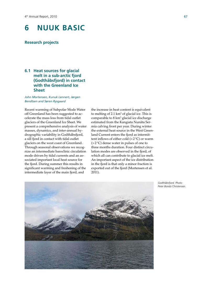
4th Annual Report, 2010 67
6 NUUK BASIC
Research projects
6.1 Heat sources for glacial melt in a sub-arctic fjord (Godthåbsfjord) in contact with the Greenland Ice Sheet
John Mortensen, Kunuk Lennert, Jørgen Bendtsen and Søren Rysgaard
Recent warming of Subpolar Mode Water off Greenland has been suggested to ac-celerate the mass loss from tidal outlet glaciers of the Greenland Ice Sheet. We present a comprehensive analysis of water masses, dynamics, and inter-annual hy-drographic variability in Godthåbsfjord, a sill fjord in contact with tidal outlet glaciers on the west coast of Greenland. Through seasonal observations we recog-nize an intermediate baroclinic circulation mode driven by tidal currents and an as-sociated important local heat source for the fjord. During summer this results in signifi cant warming and freshening of the intermediate layer of the main fjord, and
the increase in heat content is equivalent to melting of 2.1 km3 of glacial ice. This is comparable to 8 km3 glacial ice discharge estimated from the Kangiata Nunâta Ser-mia calving front per year. During winter the external heat source in the West Green-land Current enters the fjord as intermit-tent infl ows of either cold (< 2 °C) or warm (> 2 °C) dense water in pulses of one to three months duration. Four distinct circu-lation modes are observed in the fjord, of which all can contribute to glacial ice melt. An important aspect of the ice distribution in the fjord is that only a minor fraction is exported out of the fjord (Mortensen et al. 2011).
Godthåbsfjord. Photo:Peter Bondo Christensen.

4th Annual Report, 201068
6.2 Dana cruise in Godthåbs-fjord
Karen Riisgaard
On 6 June 2010 the Danish research ves-sel ‘Dana’ left the harbour of Nuuk, West Greenland, to carry out an extensive fi eld investigation on the complex interaction between climate changes and the marine food web. Twenty-two international sci-entists participated in the three-week long cruise from Fyllas Banke outside Nuuk to the inner part of Godthåbsfjord. The over-all aim for the cruise was to investigate the impact of changing climate on ocean circu-lations and biological processes in a sub-arctic marine ecosystem. As the research vessel moved into the fjord, it followed a climate gradient from high saline warm Atlantic water outside the fjord to cold water infl uenced by glacial melt water runoff in the innermost parts of the fjord. The hydrography was mapped along the transect and fi eld samples were col-lected at each station. Special emphasis was put on factors controlling vertical carbon fl uxes and the biology of selected pelagic organisms including fi sh larvae, krill, copepods, jelly fi sh, microzooplank-ton and bacteria (fi gure 6.1).
The cruise successfully collected more data than expected due to calm weather. The data collected on the cruise will be used to develop models of the circulation in the fjord and allow scientists to forecast how the system will respond to climate change. More information about the cruise, BOFYGO (Biological Oceanography at Fyl-las Banke and in Godthåbsfjord), can be found at www.aqua.dtu.dk.
6.3 The Atlantic cod (Gadus mor-hua) in Greenlandic waters: Past and future during climate change
Einar E. Nielsen, Peter Grønkjær, Mary S. Wisz, Kaj Sünksen, Rasmus Hedeholm and Nina O. Therkildsen
The marine resources in Greenland have great commercial and cultural importance for the Greenland society. The climatic changes in Greenland are expected to have a crucial effect on the future distribution and productivity of various fi sh popula-tions. One species expected to increase its Greenlandic distribution and productivity in a warmer climate is the Atlantic cod. Using a combination of genetic, biologi-cal and chemical analyses, this project at-tempts to understand and predict the population dynamics of Atlantic cod in Greenland waters. Historically, the distribution and size of the Atlantic cod population has been high-ly variable. However, knowledge of the processes governing this variability has been scarce. Firstly, fundamental know-ledge on the number of genetically and ecologically isolated populations that e-xist is needed together with investigations of whether or not these populations have separate dynamics. To address hypotheses regarding population structure, spawning cod have been sampled from both in- and offshore locations on Greenland’s east and west coast (fi gure 6.2). This provides a ge-netic baseline allowing for identifi cation of the population origin of a given individual cod. Using the Greenlandic collection of cod otoliths collected over the past century and new techniques to extract DNA from them, the population structure at various time during the past century can be com-pared to the contemporary baseline.
Figure 6.1 Sampling zooplankton onboard R/V Dana. Photo: Thomas Juul-Pedersen.

4th Annual Report, 2010 69
Another important factor in determin-ing cod productivity is feeding potential. Since preferred cod prey is known to shift distribution and productivity partly in re-sponse to climatic changes, cod producti-vity will expectedly also change. However, historical information on prey distribution is sporadic and information on actual cod prey choice is virtually absent. Using a novel technique to extract protein from the historical otoliths, the feeding of cod and possible changes are described using stab-le isotope analyses. This will document not only the trophic level of feeding but also any shift between pelagic and benthic feeding. In support of this, an extensive study on the isotopic signature of the food web along the Greenland coast has been carried out in 2010. These data on population structure and feeding, along with knowledge on cur-rent cod distribution, current climate and future climate scenarios, will be combined and used in landscape genetics. This mo-delling approach will integrate the know-ledge obtained about the system and the Atlantic cod’s response to changes. This will in turn allow for predictions on future cod populations changes in Greenland, forming the quantitative background for initiating objective precautions to ensure sustainable management of the Atlantic cod in Greenland.
6.4 Developing guidelines for sustainable whale watch-ing with special focus on humpback whales
Tenna Boye, Malene Simon and Fernando Ugarte
Whale watching is an increasing industry worldwide and in Greenland. Unregulated whale watching in Godthåbsfjord can have a short-term negative effect on humpback whale behaviour in terms of increased speed, fewer surfacing and abbreviated dives (Boye et al. 2010). Potential conse-quences of these quantifi ed behavioural changes include reduced foraging and increased energy consumption. It is not known to what extent these short term ef-fects can accumulate to long-term effects on various fi tness parameters such as skipped breeding, lower fecundity and reduced calf survival. As humpback whales are often approached closely by both commercial and private whale watching boats in Godt-håbsfjord, the aim of the study was to test a set of whale watching guidelines to help whale watching become more sustainable. From May to September 2010, the be-haviour of humpback whales and whale watching boats in Godthåbsfjord were recorded. Observations were then divided
Figure 6.2 Collecting cod specimens for sampling. Photo: Rasmus Hedeholm.

4th Annual Report, 201070
into the three categories, according to the presence and behaviour of whale watch-ing boats: undisturbed (i.e. no boats), boats following guidelines and intensive whale watching. The blow rates of humpback whales along with surfacing/dive ratio for each category were calculated (fi gure 6.3). Previous observations of blow rates and dive patterns collected in 2006-2008 were included in the data analyses to increase the number of observations as humpback whales proved hard to fi nd during 2010. Our results indicate that whales under the infl uence of intense whale watching tended to have a higher blow rate and a reduced number of surfacing before each dive as compared to undisturbed whales and whales under the infl uence of whale watching boats following guidelines. Although data was not suffi cient to make conclusive statements on the guidelines tested, the results did signify a positive outcome on whale behaviour around whale watching boats following guidelines, and based on the preliminary results we recommend the following set of guidelines:• Slow down to ‘no wake’ when within
500 m of the whale• Do not approach the whale directly
from behind or in front• Do not actively move closer to the
whale than 50 m
6.5 Climate effects on land-based ecosystems and their natural resources in Greenland
Mads C. Forchhammer and Erik Jeppesen
This project collects existing and new data on land-based ecosystems in Greenland with the objective of investigating how the expected changes in climate will affect ter-restrial and limnic ecosystems and their natural resources. Combined with data from detailed studies in West and East Greenland, respectively, we apply up-to-date analytical techniques to quantify the spatio-temporal relationships between previous changes in natural resources, their environment and climate. These data will form the basis for implementing predictive models to be used under different climate scenarios. Hence, our project will provide an assessment of future performance of land-based natural resources in a warming Arctic.
The terrestrial componentIn the projects fi rst year, 2010, efforts were primarily focused on establishment of terrestrial and limnic plots along the envi-ronmental gradient of Nuup Kangerlua. A total of 12 terrestrial sites were visited du-ring June 2010, where the landscape struc-ture and distribution of vegetation types were generally identifi ed and described.
Figure 6.3 Counting the blows of a humpback whale. Photo: Maria Iversen.

4th Annual Report, 2010 71
Furthermore, a number of samples from Salix glauca and Betula nana were collected for dendrological analysis. Based on the overall evaluation of the 12 sites, three sites were selected for long-term monitor-ing of vegetation and herbivores. Several of the dwarf shrubs sampled were over 50 years old and one even 94 years old (fi -gure 6.4), providing a unique opportunity to describe and contrast decadal and inter-annual variations in the vegetation along Nuup Kangerlua. Preliminary results indicate that there is a clear gradient from the estuary of the fjord to the Greenland Ice sheet, where the innermost sites exhibit relatively high-est annual growth. Furthermore, in years with extreme climatic conditions during winter (expressed in high or low indices of the North Atlantic Oscillation), there is an increased synchronization of vegetation growth along the entire fjord.
The limnic componentIn late summer 2010, a survey of 13 lakes was completed by an international team of scientists and students from six countries (Denmark, Spain, Brazil, Turkey, Germany and England). The aim was to provide a fi rst limnological description of the lakes and to identify food chains and biological interactions in lakes, including the use of stable isotopes. The lakes ranged in size from 0.3 to 380 ha and in depth from 0.6 m to 152 m. Water clarity was moderately high in all lakes and highest in the deep lakes, with a maximum of 11.6 m. Three of the lakes were without fi sh, one had only trout, while the rest of the lakes contained both char and three-spined stickleback. In lakes with fi sh, the catches with survey nets were very variable. Total catches in lakes ranged between 1 and 138 fi sh per net per night and for trout between 1 and 13. These results and the fi rst visual im-pression of samples taken suggest a very large effect of fi sh on the zooplankton and macro-invertebrates, on plants and in the sediment, with secondary effects on phy-toplankton (higher biomass of fi sh) and biofi lm on stone in the edge zone of the lakes (much larger biomass here if fi sh are present). The effects are far greater than we have seen in Northeast Greenland, and attributed to higher nutrient levels deter-mined by a warmer climate, which enables more extensive plant growth in lakes ba-sins and a major weathering.
Finally, sediment cores (30-80 cm of length) were sampled from the deepest of the lakes (fi gure 6.5) to analyze biological remains in the sediment in order to de-scribe changes in biodiversity and trophic structure and biological interactions in the past centuries. These samples are now be-ing processed. The ecosystem data generated at the Greenland Ecosystem Monitoring (GEM) sites, Zackenberg and Nuuk, are important components of this project and so far, one PhD has started focussing on the phenolo-gy of the terrestrial and limnic habitat sy-stems. As a novel measure of outreach, the project has its own Facebook page, where activities, results and education are an-nounced on a regular basis (http://www.facebook.com/pages/ GCRC-Projekt-6502-Landbaserede-okosystemer-ressourcer-og-klima-i- Gronland/127979750567866).
0
5
10
15
20
25
30
1910 1920 1930 1940 1950 1960 1970 1980 1990 2000 2010
Ann
ual g
row
th (
mm
*100
)
Figure 6.4 Time series of the width of annual growth rings in a Betula nana sampled at the estu-ary of Nuup Kangerlua. The individual was 94 years old.
Figure 6.5 Sediment core taken from the bottom of one of the lakes at station 1. The layered structure of the core is clearly visible. Photo: Erik Jeppesen.

4th Annual Report, 201072
7 Disturbance in the study area
Josephine Nymand
The study area at Kobbefjord is situated approximately 20 km southeast of Nuuk and can be reached by boat within half an hour. It is a public area and admittance is free to anyone. Public disturbance falls in the following categories:• Visits by boats at the bottom of the fjord
– no landing• Visits by boats at the bottom of the fjord
– the persons take a short walk inland and returns within a few hours or less.
• Visits by boats at the head of the fjord – the persons go on land and spend the night in a tent close to the coast.
• Hiking through the area – there is a hiking route from Nuuk to the inland passing through the area.
• Visits by snowmobile – during winter people visit the area from Nuuk.
• Ordinary fl ights by fi xed winged air-crafts passing over the study area in cruising altitude or in ascent or descent to or from Nuuk.
• Helicopter fl ights at cruising altitude passing over the study area.
• The electrical power transmission line between Nuuk and the hydropower plant in Buksefjord runs through the area.
In 2010, there were only few interactions between visitors in the study area and the different setups and the research hut. Foxes have been eating wires connecting temperature probes with loggers (Tiny-Tags) in the ITEX-plots; they have physi-cally moved TinyTags, moved pit-fall traps, dug up some litterbags with buried material in the Mart5, and dug holes in the ground at the very edge of Sil4. The monitoring programme itself has brought disturbance to the area i.e. trans-portation between Nuuk and the head of the fjord, housing of personnel, walking be-tween study plots and around study plots.
Transportation between Nuuk and the study site in Kobbefjord was on an irregu-lar basis, but during most of the season, there was transportation two to three times a week (mainly on Tuesdays and Thursdays). During most of the season, the research hut was used temporarily by two to four persons. Walking between the study plots has had a wearing effect on the vegetation and it should be considered to mark perma-nent trails between study sites and study plots. Portable boardwalks will be used in the future, especially around the C-fl ux measuring plots. In conclusion, it is estimated that moni-toring activities only had minor impact on the vegetation and terrain.

4th Annual Report, 2010 73
8 Logistics
Henrik Philipsen
In 2010, Greenland Institute of Natural Resources took care of the logistics re-lated to Nuuk Basic in Kobbefjord. The 2010 fi eld season in Kobbefjord was from 7 January to 16 December. During this period, 38 scientists and lo-gisticians spend approximately 360 ‘man-days’ and 75 ‘man-days’ respectively, in the study area. The winter of 2009/2010 was very mild with almost no ice in Kobbefjord. It was possible to sail to the bottom of Kob-befjord with Greenland Institute of Natu-ral Resources boats ‘Erisaalik’ and ‘Aage V. Jensen II Nuuk’ during the entire year. Greenland Institute of Natural Re-sources carried out transportation of staff, construction workers, scientists and guests from Nuuk to the study area in Kobbefjord with the boats ‘Aage V. Jensen II Nuuk’ and ‘Erisaalik’. The total number of sailing days to Kobbefjord used by Logistics, BioBasis, GeoBasis and ClimateBasis was 63 in 2010. MarineBasis used 35 sailing days to go to the study areas in Kobbefjord and Godthåbsfjord. In 2010, scientists spend 99 bed nights in the research hut in Kobbefjord. In Nuuk, the Nuuk Basic scientists were ac-commodated in the annex of Greenland Institute of Natural Resources, with 263 bed nights. Water for drinking and other purposes were taken from the nearby river. Electri-cal power was provided by two portable 2 kW gasoline generators from 2008. Communication to/from Nuuk was made by Iridium satellite telephones, while local communication within the study area was by portable VHF-radios. Aage W. Jensen’s Charity Foundation has fi nanced the two huts in Kobbefjord. The research hut has a ramp for skidoos, a terrace and 11 m² storage room under the living room. The hut is fi tted with an entrance, laboratory with hot and cold
water, bathroom with closet and shower, living room with kitchen, four berths and an oven. A generator hut houses the ge-nerator and is equipped with a ramp and a working bench. 15 April 2010, a Eurocopter AS 350 Ecureil B2 helicopter from Air Greenland made one sling with a skidoo plus one fl ight with a group of Geo- and Climate-Basis scientists from Nuuk to Kobbefjord. The scientists carried out snow monitor-ing in the area using the skidoo. 16 April 2010, the same helicopter picked up the scientists and fl ew them to Nuuk. 17-18 May 2010, minor construction work and furnishing of the two huts was carried out by two carpenters from BJ Enterprise A/S (extension and covering of the 1000 litre water tank) and logisti-cians from Greenland Institute of Natural Resources to complete the interior of the huts. 27 May 2010, Keld Hornbech Svend-sen, Asiaq – Greenland Survey, and the head of a local construction company in-spected river banks for future placement of a bridge. 1 June 2010, an Arctic fox was shot and killed after attacking a person just outside the research hut. A subsequent investiga-tion showed that the fox had rabies. In 2010, one riffl e and two fl are guns were bought for permanent use as polar bear protection in the Kobbefjord area. Fuel consumption for the generators was 40 litres of diesel and 864 litre of gaso-line. Freshwater consumption was 3200 litres. A drainpipe for grey household water was connected from 1 June until 25 Sep-tember. 256 kg non-burnable garbage was re-moved by ship to Nuuk during the season. Burnable garbage was burned on the site 25 June 2010.

4th Annual Report, 201074
The research area in Kobbefjord was du-ring 2010 visited by several honourable guests:6 May: Seven members of the Environ-
ment Committee from the Government of Greenland.
29 July: One teacher and fi ve students from the Cirius programme, Copenha-gen.
10 August: Charlotte Sahl-Madsen, Mini-ster for Science, Technology and Inno-vation, Denmark; Mimi Karlsen, Mini-ster for Culture, Education, Research and Church Affairs; Morten Meldgaard, Director of Natural History Museum of Denmark and six other attendants.
11 August: Nine teachers and PhD stu-dents with the IGERT-programme, Dartmouth, USA.
1 September: Klaus Nygaard, Director of Greenland Institute of Natural Resourc-es and two persons from Aage V. Jensen Charity Foundation.
28-30 September: One teacher and 12 stu-dents from GU (High school), Nuuk
3 October: Nine members from the board of Greenland Institute of Natural Re-sources.
22 October: 20 students from a local school in Nuuk.
Snowmobile and AS 350 helicopter in Kobbefjord, April 2010. Photo: Henrik Philipsen.

4th Annual Report, 2010 75
MarineBasis wish to acknowledge the crew onboard the R/V ‘Adolf Jensen’ for their valuable assistance during the 2010 May Cruise. We also thank Anna Haxen, Lars Heilmann, Flemming Heinrich, Kunuk Lennert, Susanne S. Hvass, Sofi e R. Jerimiassen, Sascha Schiøtt, Kaj Sünksen, Lars Witting, Finn Christensen, Andrzej Witkowski, Diana Krawczyk and Marek Zajacz-kowski for fi eld and technical assistance. MarineBasis also acknowledges Henrik Philipsen for co-ordinating the logistics of the programme.
Finally, we would like to acknowledge Morten S. Frederiksen, Carsten Egevang, Bo Bergstrøm and Ditte M. Mikkelsen for their contribution to the programme in previous years.
9 Acknowledgements

4th Annual Report, 201076
10 Personnel and visitors
Compiled by Lillian Magelund Jensen
Kristian R. Albert, Biosystems Division, Risø DTU, Denmark
Kristine E. Arendt, Greenland Climate Re-search Centre, c/o Greenland Institute of Natural Resources, Greenland
Paul Batty, Greenland Climate Research Centre, c/o Greenland Institute of Na-tural Resources, Greenland
Jørgen Bendtsen, VitusLab, DenmarkKasper Bentzen, Asiaq – Greenland Sur-
vey, GreenlandMartin Emil Blicher, Greenland Climate
Research Centre, c/o Greenland Insti-tute of Natural Resources, Greenland
Jørgen Blytmann, Asiaq – Greenland Sur-vey, Greenland
Tenna Boye, Greenland Institute of Natural Resources, Greenland
Pillunnguaq Broberg, Greenland Institute of Natural Resources, Greenland
AnnDorte Burmeister, Greenland Institute of Natural Resources, Greenland
Peter B. Christensen, National Environ-mental Research Institute, Aarhus Uni-versity, Denmark
Torben Røjle Christensen, Department of Earth and Ecosystem Sciences, Lund University, Sweden
Mikkel Lægsgaard Clausen, Asiaq – Greenland Survey, Greenland
Kristine Egede, Asiaq – Greenland Survey, Greenland
Rasmus Egede, Asiaq – Greenland Survey, Greenland
Mads C. Forchhammer, National Environ-mental Research Institute, Aarhus Uni-versity, Denmark
Jesper Fredsgaard, Asiaq – Greenland Sur-vey, Greenland
Mikkel Fruergaard, Department of Geo-graphy and Geology, University of Co-penhagen, Denmark
Arne Geisler, Greenland Institute of Natu-ral Resources, Greenland
Peter Grønkjær, Department of Biological Sciences, Aarhus University, Denmark
Per Hangaard, Asiaq – Greenland Survey, Greenland
Eric Steen Hansen, Natural History Mu-seum of Denmark, University of Co-penhagen, Denmark
Birger Ulf Hansen, Department of Geogra-phy and Geology, University of Copen-hagen, Denmark
Kristian Hassel, Norwegian University of Science and Technology, Norway
Rasmus Hedeholm, Greenland Institute of Natural Resources, Greenland
Lars Heilmann, Greenland Institute of Natural Resources, Greenland
Flemming Heinrich, Greenland Institute of Natural Resources, Greenland
Lina Hellström, Department of Earth and Ecosystem Sciences, Lund University, Sweden
Ditte Hendrichsen, National Environmen-tal Research Institute, Aarhus Univer-sity, Denmark
Karl Martin Iversen, Asiaq – Greenland Survey, Greenland
Laila Egede Ignatiussen, Asiaq – Green-land Survey, Greenland
Lillian Magelund Jensen, National Envi-ronmental Research Institute, Aarhus University, Denmark
Erik Jeppesen, National Environmental Research Institute, Aarhus University, Denmark
Henrik Fenger Jeppesen, Asiaq – Green-land Survey, Greenland
Aqqalu Josefsen, Asiaq – Greenland Sur-vey, Greenland
Thomas Juul-Pedersen, Greenland Climate Research Centre, c/o Greenland Insti-tute of Natural Resources, Greenland
Rasmus H. Jørgensen, LIFE, University of Copenhagen, Denmark
Nanna Kandrup, Asiaq – Greenland Sur-vey, Greenland
Dorte Krause-Jensen, National Environ-mental Research Institute, Aarhus Uni-versity, Denmark
Aili Labansen, Institute of Natural Re-sources, Greenland
Morten Larsen, Asiaq – Greenland Survey, Greenland

4th Annual Report, 2010 77
Torben L. Lauridsen, National Environ-mental Research Institute, Aarhus Uni-versity, Denmark
Kunuk Lennert, Greenland Climate Re-search Centre, c/o Greenland Institute of Natural Resources, Greenland
Magnus Lund, National Environmental Research Institute, Aarhus University, Denmark
Winnie Martinsen, National Environmen-tal Research Institute, Aarhus Univer-sity, Denmark
Núria Marbà, Department of Global Change Research, IMEDEA (CSIC-UIB), Institut Mediterrani d’Estudis Avançats, Spain
Mikhail Mastepanov, Department of Earth and Ecosystem Sciences, Lund Univer-sity, Sweden
Mikkel Christian Mikkelsen, Asiaq – Greenland Survey, Greenland
John Mortensen, Greenland Climate Re-search Centre, c/o Greenland Institute of Natural Resources, Greenland
Jacob Nabe-Nielsen, National Environ-mental Research Institute, Aarhus Uni-versity, Denmark
Martin Nauta, Asiaq – Greenland Survey, Greenland
Einar E. Nielsen, National Institute of Aquatic Resources, DTU Aqua, Den-mark
Rasmus Nygaard, Greenland Institute of Natural Resources, Greenland
Josephine Nymand, Greenland Institute of Natural Resources, Greenland
Bo Naamansen, Asiaq – Greenland Survey, Greenland
Birgit Olesen, Institute of Biology, Aarhus University, Denmark
Stine Højlund Pedersen, Department of Geography and Geology, University of Copenhagen, Denmark
Mark Andrew Pernosky, Asiaq – Green-land Survey, Greenland
Dorthe Petersen, Asiaq– Greenland Sur-vey, Greenland
Jonathan N. K. Petersen, Asiaq – Green-land Survey, Greenland
Henrik Philipsen, Greenland Institute of Natural Resources, Greenland
Tommy Prestø, Norwegian University of Science and Technology, Norway
Morten Rasch, National Environmental Research Institute, Aarhus University, Denmark
Bo Holm Rasmussen, Department of Geo-graphy and Geology, University of Co-penhagen, Denmark
Lars M. Rasmussen, Greenland Institute of Natural Resources, Greenland
Katrine Raundrup, Greenland Institute of Natural Resources, Greenland
Anja Retzel, Greenland Institute of Natu-ral Resources, Greenland
Karen Riisgaard, National Institute for Aquatic Resources, DTU Aqua
Søren Rysgaard, Greenland Climate Re-search Centre, c/o Greenland Institute of Natural Resources, Greenland
Niels Martin Schmidt, National Environ-mental Research Institute, Aarhus Uni-versity, Denmark
Mikael K. Sejr, National Environmental Research Institute, Aarhus University, Denmark
Charlotte Sigsgaard, Department of Geo-graphy and Geology, University of Co-penhagen, Denmark
Malene Simon, Greenland Climate Re-search Centre, c/o Greenland Institute of Natural Resources, Greenland
Lena Ström, Department of Earth and Ecosystem Sciences, Lund University, Sweden
Kaj Sünksen, Greenland Institute of Natu-ral Resources, Greenland
Mikkel P. Tamstorf, National Environmen-tal Research Institute, Aarhus Univer-sity, Denmark
Nina O. Therkildsen, National Institute of Aquatic Resources, DTU Aqua, Denmark
Kisser Thorsøe, Asiaq - Greenland Survey, Greenland
Anders Westergaard-Nielsen, Department of Geography and Geology, University of Copenhagen, Denmark
Mary S. Wisz, National Environmental Research Institute, Aarhus University, Denmark
Lars Witting, Greenland Institute of Natu-ral Resources, Greenland
Peter Aastrup, National Environmental Research Institute, Aarhus University, Denmark
Please notice that the list of visitors is not complete as the Greenland Institute of Natural Resources has stopped their regi-stration of visitors.

4th Annual Report, 201078
11 Publications
Scientifi c papers
Arendt, K.E., Nielsen, T.G., Rysgaard, S. and Tönneson, K. 2010. Differences in plankton community structure along Godthåbsfjord; from the Greenland Ice Sheet to offshore waters, SW Green-land. Marine Ecology Progress Series 401:49-62.
Blicher, M.E., Clemmesen, C., Rysgaard, S., Sejr, M.K. and Mempel, H. 2010. Seasonal and spatial variations in the RNA:DNA ratio and its relation to growth for sub-Arctic scallops. Marine Ecology Progress Series 407:87-98.
Blicher, M.E., Sejr, M.K. and Rysgaard, S. 2010. Seasonal growth variation of Chla-mys islandica (Bivalvia) in the sub-Arctic Greenland is linked to food availability and temperature. Marine Ecology Pro-gress Series 407:71-86.
Boye, T.K., Simon, M. and Madsen, P.T. 2010. Habitat use of humpback whales in Godthåbsfjord, West Greenland, with implications for commercial exploita-tion. Journal of the Marine Biological Association of the United Kingdom. doi:10.1017/S0025315410000755.
Glud, R.N., Berg, P., Hume, A., Batty, P., Blicher, M.E., Lennert, K. and Rys-gaard, S. 2010. Benthic O2 exchange rates across hard-bottom sediments as quantifi ed by eddy correlation in a sub-Arctic fjord system. Marine Ecology Progress Series 417:1-12.
Hedeholm, R., Grønkjær, P., Rosing-Asvid, A. and Rysgaard, S. 2010. Variation in size and growth of West Greenland capelin (Mallotus villosus) along a latitu-dinal gradient. ICES Journal of Marine Science. Doi:10.1093/icesjms/fsq024.
Mikkelsen, D.M. and Witkowski, A. 2010. Melting sea ice for taxonomic analysis: a comparison of four melting proce-dures. Polar Research 29: 451-454.
Piña-Ochoa, E., Høgslund, S., Geslin, E., Cedhagen, T., Revsbech, N.P., Nielsen, L.P., Schweiger, M., Jorissen, F., Rysgaard, S. and Risgaard-Petersen, N. 2010. Wide-spread occurrence of nitrate storage and denitrifi cation among Foraminifera and Gromiida. Proceedings of the National Academy of Sciences 107:1148-1153.
Post, E., Forchhammer, M.C., Tyler, N.J.C., Høye, T.T., Tamstorf, M.P., Christensen, T.R., Elberling, B., Gilg, O., Hik, D.S., Ims, R.A., Rysgaard, S., Stirling, I., Wel-ker, J., Wookey, P.A., Schmidt, N.M. and Aastrup, P. 2010. Response to B. Griffi th et al.'s E-Letter. 13 January 2010. Science.
Ruiz-Halpern, S., Sejr, M.K., Duarte, C.M., Krause-Jensen, D., Dalsgaard, T., Dachs, J. and Rysgaard, S. 2010. Air-water ex-change and vertical profi les of organic carbon in a subarctic fjord. Limnology and Oceanography 55:1733-1740.
Søgaard, D.H., Kristensen, M., Rysgaard, S. and Glud, R.N. 2010. Dynamics of autotrophic and heterotrophic activity in Arctic fi rst-year sea ice: Case study from Marlene Bight, SW Greenland. Marine Ecology Progress Series 419:31-45.
ReportsAndreasen, R.H. 2010: Infl uences on a low
arctic ecosystem from spatiotemporal variations of insolation, soil moisture and temperature. Master thesis at De-partment of Geography and Geology, University of Copenhagen. 60 pp.
Blicher, M.E. 201 0. Structure and dynamics of marine macrozoobenthos in Green-land – and the link to environmental drivers. PhD thesis. Greenland Institute of Natural Resources & Department for Biology, University of Copenhagen. Greenland Institute of Natural Resour-ces, 162 pp.
Pedersen, S.H. 2010: Global radiation in Nuuk and Kobbefjord SW Greenland. Bachelor thesis at Department of Ge-ography and Geology, University of Copenhagen. 62 pp.

4th Annual Report, 2010 79
Rysgaard, S. 2010. Coastal Environments as a link between land and sea in the Arctic. IASC 08/09 Bulletin. Interna-tional Arctic Science Committee. Rachold V., Bowden S. and Pit M. (eds). ISSN:1654-7594. pp 48-49.
Westergaard-Nielsen, A. 2010. Piselating Plants – Spatial temporal monitoring of phenology and snow cover dyna-mics in Arctic using unmodifi ed digital cameras. Master thesis at Department of Geography and Geology, University of Copenhagen. 90 pp.
Presentation at symposiums, work-shops, meetings and conferencesBatty, P. Oral presentation: ATP meeting in
Napoli, Italy. 8 July 2010.Blicher, M.E. 2010. PhD Defence: Structure
and dynamics of marine macrozoo-benthos in Greenland – and the link to environmental drivers. Marine Biological Laboratory, Department for Biology, Uni-versity of Copenhagen. 18 August, 2010.
Juul-Pedersen, T. and Rysgaard, S., Oral presentation : French days in Nuuk. Open scientifi c seminar. Ilisimartusarfi k, Nuuk, Greenland, 28 May 2010.
Juul-Pedersen, T. Oral presentation: SIN-TEF seminar on Oil Spill response for Arctic and ice covered waters, Nuuk, Greenland, 24 August 2010.
Juul-Pedersen, T. Oral presentation/edu-cation: Nordisk Klimadag 2010, Nuuk, Greenland, 22 Oktober, 2010.
Krause-Jensen, D., Marbà, N., Olesen, B., Christensen, P.B., Sejr, M. and Rodri-gues, J., Rysgaard, S., 2011. Oral pre-sentation: Benthic marine vegetation in Greenland – response to climate for-cing. Arctic Frontiers Conference. Trom-sø, Norway, 24-28 January, 2011.
Mikkelsen, P.S. Oral presentation: Climate research in Greenland / Greenland Cli-mate Research Centre. “The World”, 13. September, 2010.
Rasmussen, L.M., Blicher, M.E., Sejr, M.K., Merkel, F.R. and Rysgaard, S. 2010. Poster: Evidence for strong trophic coupling between macrozoobenthos and wintering eiders (Somateria spp.) in a shallow sub-Arctic sound. 1st World Seabird Conference, Victoria, Canada, 7-11 September, 2010.
Rysgaard, S. 2010. Oral presentation: Arctic tipping Points – An example of cooperation and initiation of a research project funded by the European Union 7th Framework Programme. Greenland Tourism & Business Council meeting in Nuuk, Greenland, 3 March, 2010.
Rysgaard, S. 2010. Oral presentation: 17th Conference on Air-Sea Interaction, 17th Conference on Satellite Meteorology and Oceanography, Ninth Conference on Coastal Atmospheric and Oceanic Prediction and Processes, Annapolis, USA, 27 September-1 October, 2010.
Rysgaard, S. 2010. Oral presentation: At the front steps of Climate change, Sy-nergy effects of climate cooperation on research in Arctic, case; Greenland and Canada, “Research & Development in and for the Arctic – Greenland”, EU Parliament, Bruxelles, 26 October, 2010.
Rysgaard, S. 2010. Oral presentation: Greenland Climate research Centre – New initiatives and ongoing activities. Arctic Science Summit Week, Nuuk, Greenland, 15-18 April, 2010.
Søgaard, D.H. 2010. Oral presentation: IPY om alger og bakterier i havisen, Oslo, Norway, 11 Juni, 2010.
Versteegh, E.A.A., Blicher, M.E., Troelstra, S.R. and Dehairs, F. 2010. Oral presenta-tion: Bivalve sclerochemistry as a proxy for past Greenland melt water runoff. 2nd International Sclerochronology Confe-rence, Mainz, Germany, 24-28 July, 2010.
General informationJuul-Pedersen, T. Go North! Internet chat
event with schools from around the world. Theme: “World Resources”, Topic: “Ecology: Sustainable Develop-ment”. 23 April, 2010.
Mikkelsen, P.S., Juul-Pedersen, T. and Batty, P. ICC Event – GCRC Stand. 28 June - 2 July, 2010.
Mikkelsen, P.S. and Juul-Pedersen, T. Cli-mate change in Greenland. Taiwan TV. 15 September, 2010.
Rysgaard, S. KNR radio. Havis og dets rolle i kuldioxidoptaget fra atmosfæren. 23 Januar, 2010.
Rysgaard, S. Al Jazeera TV. September 2010.
Rysgaard, S. YouTube – Life in the sea ice. www.youtube.com. 17 May, 2010.

4th Annual Report, 201080
12 References
Bay, C., Aastrup, P. and Nymand, J. 2008. The NERO line: A vegetation transect in Kobbefjord, West Greenland. National Environmental Research Institute, Aarhus University, Denmark. NERI Technical Report no. 693. 40 pp.
Blicher, M.E., Rysgaard, S. and Sejr, M.K. 2010. Seasonal growth variation in Chla-mys islandica (Bivalvia) from sub-Arctic Greenland is linked to food availability and temperature. Marine Ecology Pro-gress Series 407:71-86.
Blicher, M.E., Sejr, M.K. and Rysgaard, S. 2009. High carbon demand of dominant macrozoobenthic species indicates their central role in ecosystem carbon fl ow in a sub-Arctic fjord. Marine Ecology Pro-gress Series 383:127-140.
Born, E., Rysgaard, S., Ehlmé, G., Sejr, M., Acquarone, M. and Levermann, N. 2003. Underwater observations of foraging free-living Atlantic walruses (Odobenus rosmarus) and estimates of their food consumption. Polar Biology 26:348-357.
Borum, J., Pedersen, M.F., Krause-Jensen, D., Christensen, P.B. and Nielsen, K. 2002. Biomass, Photosynthesis and Growth of Laminaria saccharina in a High-Arctic Fjord, NE Greenland. Ma-rine Biology 141:11-19.
Boye, T.K., Simon, M. and Madsen, P.T. 2010. Habitat use of humpback whales in Godthåbsfjord, West Greenland, with implications for commercial exploita-tion. Journal of the Marine Biological Association of the United Kingdom 90:1529-1538.Cappelen, J., Jørgensen, B.V., Laursen, E.V., Stannius, L.S. and Thomsen, R.S. 2001. Technical Report 00-18. The Ob-served Climate of Greenland, 1958-99 – with Climatological Standard Normals, 1961-90. ISSN 0906-897.
Carstensen, L.S. and Jørgensen, B.V. 2011. Weather and Climate Data from Green-land 1958-2010, Dataset available for research and educational purposes. Descriptions and Documentation of Observations of Temperature, Precipita-tion, Wind, Cloud Cover, Air Pressure, Humidity and Depth of Snow, DMI, Technical report 11-10.
Dunton, K.H. 1985. Growth of dark-exposed Laminaria saccharina (L.) Lamour and of Laminaria solidungula J. Ag. (Laminarales: Phaeophyta) in the Alaskan Beaufort Sea. Journal of Ex-perimental Marine Biology and Ecology 94:181-189.
Gattuso, J.-P., Gentili, B., Duarte, C.M., Kleypas, J.A., Middelburg, J.J. and An-toine, D. 2006. Light availability in the coastal ocean: impact on the distribu-tion of benthic photosynthetic orga-nisms and their contribution to primary production. Biogeosciences 3:489-513.
Gómez, I., Wulff, A., Roleda, M.Y., Huovinen, P., Karsten, U., Quartino, M.L., Dunton, K. and Wiencke, C. 2009. Light and temperature demands of ma-rine benthic microalgae and seaweeds in polar regions. Botanica Marina 52:593-608.
Hansen B.U., Iversen, K.M., Tamstorf, M.P., Sigsgaard, C., Fruergaard, M., Højlund, S., Lund, M., Raundrup, K., Mastepanov, M., Falk, J.M., Ström, L., Westergaard, A., Rasmussen, B.H. and Christensen T.R. 2009. Nuuk Basic: The GeoBasis Programme. In Jensen, L.M. and Rasch, M. (eds.). Nuuk Ecologi-cal Research Operations, 3rd Annual Report, 2010. National Environmental Research Institute, Aarhus University, Denmark. 80 pp.
Heide-Jørgensen, M.P. and Laidre, K.L. 2007. Autumn space-use patterns of humpback whales (Megaptera novaean-gliae) in West Greenland. Journal of Ce-tacean Research Management 9:121-128.

4th Annual Report, 2010 81
Heide-Jørgensen, M.P., Laidre, K.L., Han-sen, R.G., Rasmussen, M., Burt, M.L., Borchers, D.L., Dietz, R. and Teilmann, J. 2008. Revised abundance estimates of humpback whales in West Greenland. Report of the International Whaling Commission SC/60/AWMP7: 1-35.
ISO 1100-2 1998. Measurement of liquid fl ow in open channels – Part 2: Deter-mination of stage-discharge relation, ISO 1100-2, International Organization for Standardization, Switzerland 1998.
Jensen, J.P., Lauridsen, T.L., Søndergaard, M., Jeppesen, E., Agerbo, E. and Sort-kjær, L. 1996. Ferske vandområder – Søer. Vandmiljøplanens overvågnings-program 1995. Technical Report no. 176, National Environmental Research Institute, Aarhus University, Denmark. 96 pp.
Jensen, L.M. and Rasch, M. (eds.) 2010. Nuuk Ecological Research Operations, 3rd Annual Report, 2009. National En-vironmental Research Institute, Aarhus University, Denmark. 80 pp.
Jensen, L.M and Rasch, M. (eds.) 2009. Nuuk Ecological Research Operations, 2nd Annual Report, 2008. National En-vironmental Research Institute, Aarhus University, Denmark. 80 pp.
Jensen, L.M and Rasch, M. (eds.) 2008. Nuuk Ecological Research Operations, 1st Annual Report, 2007. Copenhagen, Danish Polar Centre, Danish Agency for Science, Technology and Innovation, Ministry of Science, Technology and In-novation, 2008. 112 pp.
Juul-Pedersen, T., Rysgaard, S., Batty, P., Mortensen, J., Retzel, A., Nygaard, R., Burmeister, A., Mikkelsen, D.M., Sejr, M.K., Blicher, M.E., Krause-Jensen, D., Christensen, P.B., Labansen, A.L., Ras-mussen, L.M., Simon, M., Boye, T.K., Madsen, P.T. and Ugarte, F. 2009. Nuuk Basic: The MarineBasis programme. In Jensen, L.M. and Rasch, M. (eds.) 2009. Nuuk Ecological Research Operations, 2nd Annual Report, 2008. National En-vironmental Research Institute, Aarhus University, Denmark. 80 pp.
Katona, S.K., Baxter, B., Brazier, O., Kraus, S., Perkins, J. and Whitehead, H. 1979. Identifi cation of humpback whales by fl uke photographs. In: Winn, H. E. and Olla, B.L. (eds). The behaviour of marine animals. Volume 3. Cetacea. Ple-num Press, New York. 438 pp.
Lund, S. 1951. Marine algae from Jørgen Brøndlunds Fjord in eastern North Greenland. Meddelelser om Grønland 128:1-26.
Mann, K.H. 1973. Seaweeds: their produc-tivity and strategy for growth. Science 182:975-981.
Merkel, F.R., Jamieson, S.E., Falk K. and Mosbech A. 2007. The diet of common eiders wintering in Nuuk, Southwest Greenland. Polar Biology 30:227-234.
Mortensen, J., Lennert, K., Bendtsen, J. and Rysgaard, S. 2011. Heat sources for glacial melt in a sub-arctic fjord (Godt-håbsfjord) in contact with the Green-land Ice Sheet, J. Geophysics. Res. 116, C01013, doi:10.1029/2010JC006528.
Sejr, M., Włodarska-Kowalczuk, M., Legeżyńska, J. and Blicher, M. 2010. Macrobenthic species composition and diversity in the Godthåbsfjord system, SW Greenland. Polar Biology 33:421-431.
Rysgaard, S. and Glud, R.N. (eds.) 2007. Carbon cycling in Arctic marine eco-systems; Case study Young Sund. Med-delelser om Grønland, Bioscience 58. The Commission for Scientifi c Research in Greenland. 214 pp.
Tamstorf, M.P., Iversen, K.M., Hansen B.U., Sigsgaard, C., Fruergaard, M., Højlund, S., Andreasen, R.H., Mastepanov, M., Falk, J.M., Ström, L. and Christensen T.R. 2009. Nuuk Basic: The GeoBasis Programme. In Jensen, L.M. and Rasch, M. (Eds.). Nuuk Ecological Research Op-erations, 2nd Annual Report, 2008. Na-tional Environmental Research Institute, Aarhus University, Denmark. 80 pp.
Aastrup, P., Nymand, J., Raundrup, K., Lauridsen, T.L., Krogh, P.H., Schmidt, N.M., Illeris, L. and Ro-Poulsen, H. 2009. Conceptual design and sampling procedures of the biological program-me of Nuuk Basic. National Environ-mental Research Institute, Aarhus University, Denmark. NERI Technical Report No. 745. 77 pp.

4th Annual Report, 201082
13 Appendix
Day-of-year (DOY)
Regular years
Jan Feb Mar Apr May Jun Jul Aug Sep Oct Nov Dec
1 1 32 60 91 121 152 182 213 244 274 305 335
2 2 33 61 92 122 153 183 214 245 275 306 336
3 3 34 62 93 123 154 184 215 246 276 307 337
4 4 35 63 94 124 155 185 216 247 277 308 338
5 5 36 64 95 125 156 186 217 248 278 309 339
6 6 37 65 96 126 157 187 218 249 279 310 340
7 7 38 66 97 127 158 188 219 250 280 311 341
8 8 39 67 98 128 159 189 220 251 281 312 342
9 9 40 68 99 129 160 190 221 252 282 313 343
10 10 41 69 100 130 161 191 222 253 283 314 344
11 11 42 70 101 131 162 192 223 254 284 315 345
12 12 43 71 102 132 163 193 224 255 285 316 346
13 13 44 72 103 133 164 194 225 256 286 317 347
14 14 45 73 104 134 165 195 226 257 287 318 348
15 15 46 74 105 135 166 196 227 258 288 319 349
16 16 47 75 106 136 167 197 228 259 289 320 350
17 17 48 76 107 137 168 198 229 260 290 321 351
18 18 49 77 108 138 169 199 230 261 291 322 352
19 19 50 78 109 139 170 200 231 262 292 323 353
20 20 51 79 110 140 171 201 232 263 293 324 354
21 21 52 80 111 141 172 202 233 264 294 325 355
22 22 53 81 112 142 173 203 234 265 295 326 356
23 23 54 82 113 143 174 204 235 266 296 327 357
24 24 55 83 114 144 175 205 236 267 297 328 358
25 25 56 84 115 145 176 206 237 268 298 329 359
26 26 57 85 116 146 177 207 238 269 299 330 360
27 27 58 86 117 147 178 208 239 270 300 331 361
28 28 59 87 118 148 179 209 240 271 301 332 362
29 29 88 119 149 180 210 241 272 302 333 363
30 30 89 120 150 181 211 242 273 303 334 364
31 31 90 151 212 243 304 365

4th Annual Report, 2010 83
Day-of-year (DOY)
Leap years Jan Feb Mar Apr May Jun Jul Aug Sep Oct Nov Dec
1 1 32 61 92 122 153 183 214 245 275 306 336
2 2 33 62 93 123 154 184 215 246 276 307 337
3 3 34 63 94 124 155 185 216 247 277 308 338
4 4 35 64 95 125 156 186 217 248 278 309 339
5 5 36 65 96 126 157 187 218 249 279 310 340
6 6 37 66 97 127 158 188 219 250 280 311 341
7 7 38 67 98 128 159 189 220 251 281 312 342
8 8 39 68 99 129 160 190 221 252 282 313 343
9 9 40 69 100 130 161 191 222 253 283 314 344
10 10 41 70 101 131 162 192 223 254 284 315 345
11 11 42 71 102 132 163 193 224 255 285 316 346
12 12 43 72 103 133 164 194 225 256 286 317 347
13 13 44 73 104 134 165 195 226 257 287 318 348
14 14 45 74 105 135 166 196 227 258 288 319 349
15 15 46 75 106 136 167 197 228 259 289 320 350
16 16 47 76 107 137 168 198 229 260 290 321 351
17 17 48 77 108 138 169 199 230 261 291 322 352
18 18 49 78 109 139 170 200 231 262 292 323 353
19 19 50 79 110 140 171 201 232 263 293 324 354
20 20 51 80 111 141 172 202 233 264 294 325 355
21 21 52 81 112 142 173 203 234 265 295 326 356
22 22 53 82 113 143 174 204 235 266 296 327 357
23 23 54 83 114 144 175 205 236 267 297 328 358
24 24 55 84 115 145 176 206 237 268 298 329 359
25 25 56 85 116 146 177 207 238 269 299 330 360
26 26 57 86 117 147 178 208 239 270 300 331 361
27 27 58 87 118 148 179 209 240 271 301 332 362
28 28 59 88 119 149 180 210 241 272 302 333 363
29 29 60 89 120 150 181 211 242 273 303 334 364
30 30 90 121 151 182 212 243 274 304 335 365
31 31 91 152 213 244 305 366

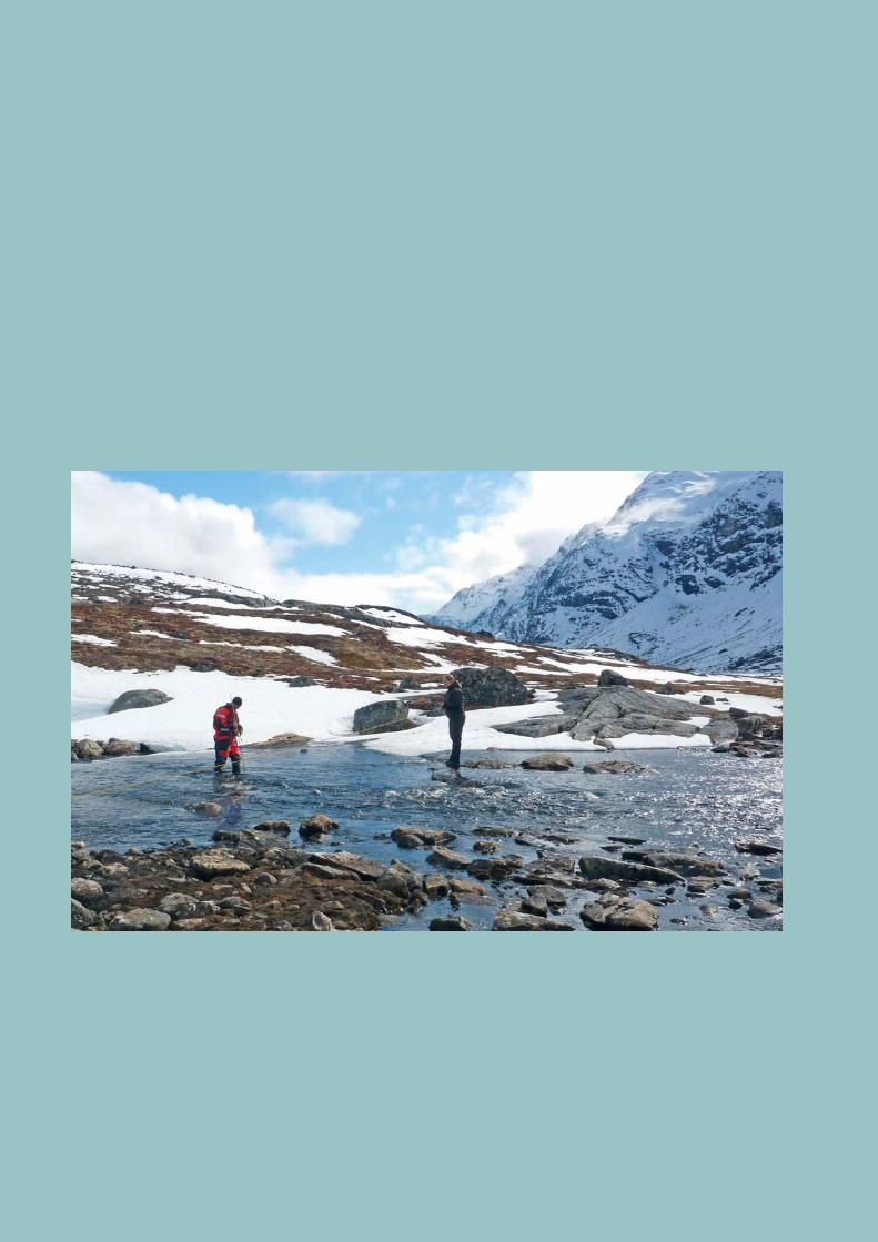
4th Annual Report 2010
Aarhus UniversityDCE – Danish Centre for Environment and Energy
NER
O – 4
th Annua
l Re
po
rt 2010