Workshop on Advanced Techniques for Scientific Programming and Management of Open Source Software Packages 10–21 March 2014

NumPy, SciPy and Matplotlib

David Grellscheid with thanks to Shawn Brown, Pittsburgh Supercomputing Center

What are NumPy and SciPy?

• NumPy and SciPy are open-source add-on modules to Python that provide common mathematical and numerical routines in pre- compiled, fast functions.

• The NumPy (Numeric Python) package provides basic routines for manipulating large arrays and matrices of numeric data.

• The SciPy (Scientific Python) package extends the functionality of NumPy with a substantial collection of useful algorithms, like minimization, Fourier transformation, regression, and other applied mathematical techniques.

Installation of NumPy and SciPy

• They are listed on PyPI, so can be installed with “pip install numpy scipy”

• http://www.scipy.org/install.html has other alternatives

Using the modules

Import the modules into your program like most Python packages:

import numpy !import numpy as np !from numpy import *

import scipy !import scipy as sp !from scipy import *

The Array• The array is the basic, essential unit of NumPy

– Designed to be accessed just like Python lists

– All elements are of the same type

– Ideally suited for storing and manipulating large numbers of elements

>>> a = np.array([1, 4, 5, 8], float32) !>>> a array([1., 4., 5., 8.]) !>>> type(a)<type ‘numpy.ndarray’>

>>> a[:2] Array([1., 4.]) !>>> a[3] 8.0

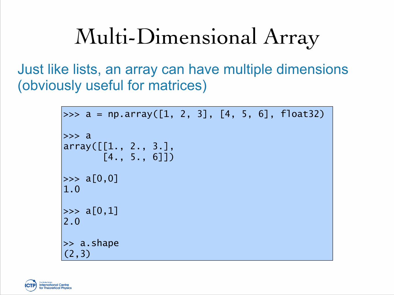
Multi-Dimensional ArrayJust like lists, an array can have multiple dimensions (obviously useful for matrices)

>>> a = np.array([1, 2, 3], [4, 5, 6], float32) !>>> aarray([[1., 2., 3.], [4., 5., 6]]) !>>> a[0,0] 1.0 !>>> a[0,1] 2.0 !>> a.shape (2,3)

Multi-Dimensional ArrayArrays can be reshaped:

>>> a = np.array(range(10), float32) >>> aarray([ 0., 1., 2., 3., 4., 5., 6., 7., 8., 9.]) !>>> a.reshape((5, 2)) >>> aarray([ 0., 1., 2., 3., 4., 5., 6., 7., 8., 9.]) !>>> b = a.reshape((5,2)) array([[ 0., 1.], [ 2., 3.], [ 4., 5.], [ 6., 7.], [ 8., 9.]]) !>>> b.shape (5, 2)

b points at same data in memory,

new “view”

Views and copiesPlain assignment creates a view, copies need to be explicit:

>>> a = np.array([1, 2, 3], float) >>> b = a>>> c = a.copy() !>>> a[0] = 0 !>>> a array([0., 2., 3.]) !>>> b array([0., 2., 3.]) !>>> carray([1., 2., 3.])

Other array operations• One can fill an array with a single value

• Arrays can be transposed easily

!>>> a = np.array([1, 2, 3],float) !>>> a array([1.0, 2.0, 3.0]) !>>> a.fill(0) array([0.0, 0.0, 0.0]) !>>> a = np.array(range(6), float).reshape((2, 3)) >>> aarray([[ 0., 1., 2.], [ 3., 4., 5.]]) !>>> a.transpose() array([[ 0., 3.], [ 1., 4.], [ 2., 5.]])

Array concatenation

Combining arrays can be done through concatenation

>>> a = np.array([1,2], float) >>> b = np.array([3,4,5,6], float) >>> c = np.array([7,8,9], float) >>> np.concatenate((a, b, c)) array([1., 2., 3., 4., 5., 6., 7., 8., 9.])

Array concatenationMulti-dimensional arrays can be concatenated along a specific axis:

>>> a = np.array([[1, 2], [3, 4]], float) >>> b = np.array([[5, 6], [7, 8]], float) !>>> np.concatenate((a,b),axis=0)array([[ 1., 2.], [ 3., 4.], [ 5., 6.], [ 7., 8.]]) !>>> np.concatenate((a,b),axis=1) array([[ 1., 2., 5., 6.], [ 3., 4., 7., 8.]]

Other ways to create arrays>>> np.arange(5, dtype=float) array([ 0., 1., 2., 3., 4.]) !>>> np.linspace(30,40,5) array([ 30. , 32.5, 35. , 37.5, 40. ]) !>>> np.ones((2,3), dtype=float) array([[ 1., 1., 1.], [ 1., 1., 1.]]) >>> np.zeros(7, dtype=int) array([0, 0, 0, 0, 0, 0, 0]) !>>> a = np.array([[1, 2, 3], [4, 5, 6]], float) >>> np.zeros_like(a) array([[ 0., 0., 0.], [ 0., 0., 0.]]) >>> np.ones_like(a) array([[ 1., 1., 1.], [ 1., 1., 1.]])

The power of NumPy

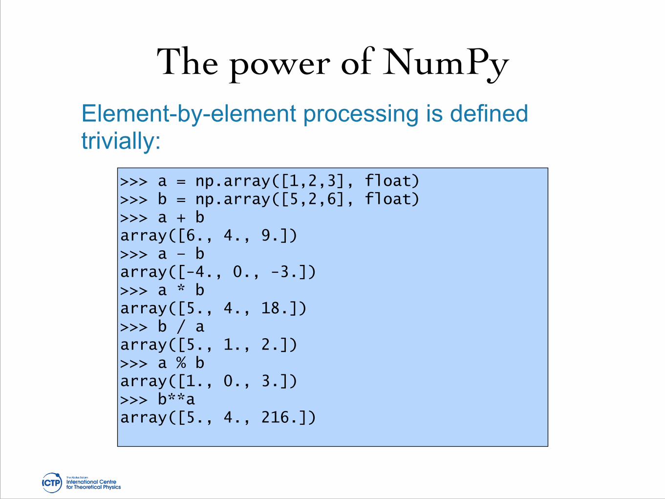
>>> a = np.array([1,2,3], float) >>> b = np.array([5,2,6], float) >>> a + barray([6., 4., 9.]) >>> a – barray([-4., 0., -3.]) >>> a * barray([5., 4., 18.]) >>> b / aarray([5., 1., 2.]) >>> a % barray([1., 0., 3.]) >>> b**aarray([5., 4., 216.])

Element-by-element processing is defined trivially:

The power of NumPy

>>> a = np.array([[1, 2], [3, 4], [5, 6]], float) >>> b = np.array([-1, 3], float) >>> aarray([[ 1., 2.], [ 3., 4.], [ 5., 6.]]) >>> b array([-1., 3.]) !>>> a + b array([[ 0., 5.], [ 2., 7.], [ 4., 9.]])

Watch out for automatic shape extension:

b was extended to match shape (3,2):

array([[ -1., 3.], [ -1., 3.], [ -1., 3.]])

The power of NumPy

>>> a = np.zeros((2,2), float) array([[ 0., 0.], [ 0., 0.]]) >>> b = np.array([-1., 3.], float) array([-1., 3.]) !>>> a + b array([[-1., 3.], [-1., 3.]]) !>>> a + b[np.newaxis,:] array([[-1., 3.], [-1., 3.]]) !>>> a + b[:,np.newaxis] array([[-1., -1.], [ 3., 3.]])

Control shape extension with newaxis:

Array mathsNumPy offers a large library of common mathematical functions that can be applied elementwise to arrays

– Among these are: abs, sign, sqrt, log, log10, exp, sin, cos, tan, arcsin, arccos, arctan, sinh, cosh, tanh, arcsinh, arccosh, and arctanh

>>> a = np.linspace(0.3,0.6,4) array([ 0.3, 0.4, 0.5, 0.6, 0.7]) !>>> np.sin(a) >>> array([ 0.29552021, 0.38941834, 0.47942554, 0.56464247])

Array statistics

>>> a = np.array([2, 4, 3], float) >>> a.sum() 9.0 >>> a.prod() 24.0!>>> np.sum(a) 9.0 >>> np.prod(a) 24.0 !>>> a = np.array([2, 1, 9], float) >>> a.mean()4.0>>> a.var() 12.666666666666666 >>> a.std() 3.5590260840104371

Array statistics

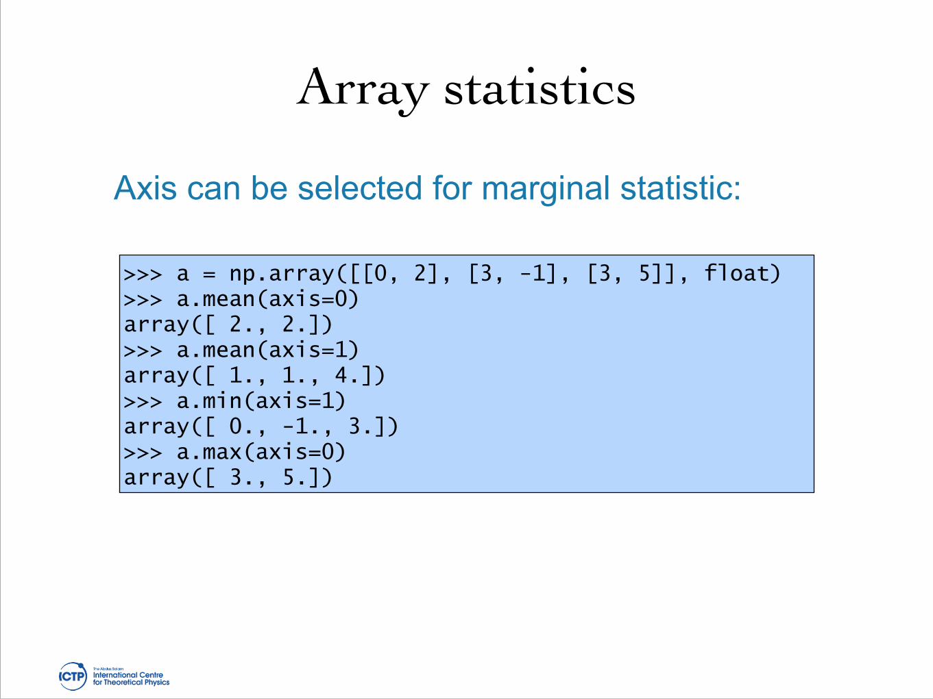
>>> a = np.array([[0, 2], [3, -1], [3, 5]], float) >>> a.mean(axis=0) array([ 2., 2.]) >>> a.mean(axis=1) array([ 1., 1., 4.]) >>> a.min(axis=1) array([ 0., -1., 3.]) >>> a.max(axis=0) array([ 3., 5.])

Axis can be selected for marginal statistic:

Boolean arrays

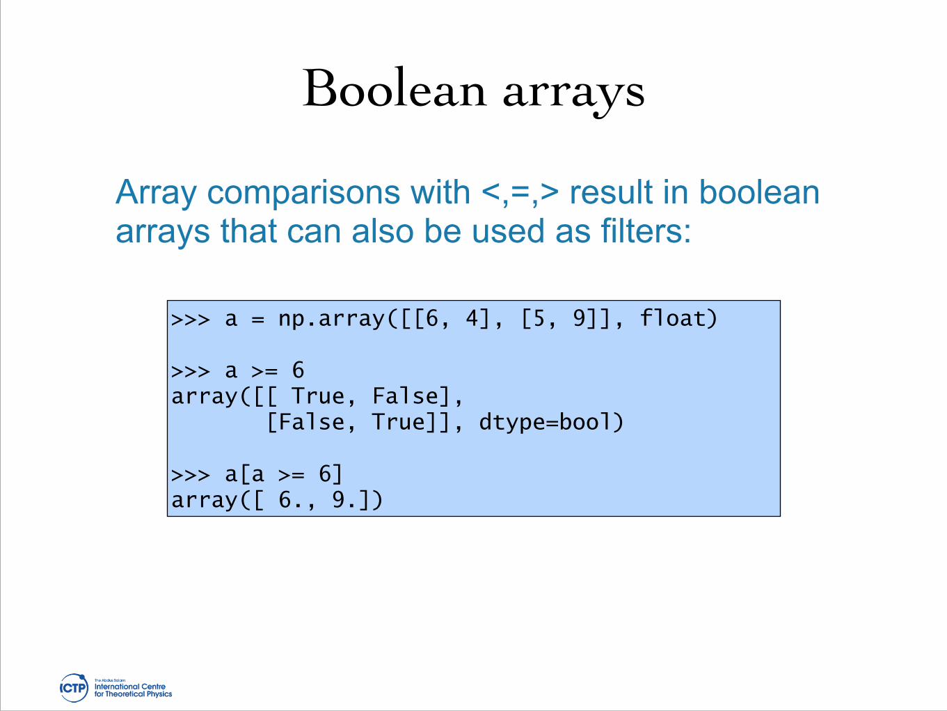
>>> a = np.array([[6, 4], [5, 9]], float) !>>> a >= 6 array([[ True, False], [False, True]], dtype=bool) !>>> a[a >= 6] array([ 6., 9.])

Array comparisons with <,=,> result in boolean arrays that can also be used as filters:

Linear Algebra

• Perhaps the most powerful feature of NumPy is the vector and matrix operations

– Provide compiled code performance similar to machine specific BLAS, uses BLAS internally

• Performing a vector-vector, vector-matrix or matrix-matrix multiplication using dot

• Also supports inner, outer, cross

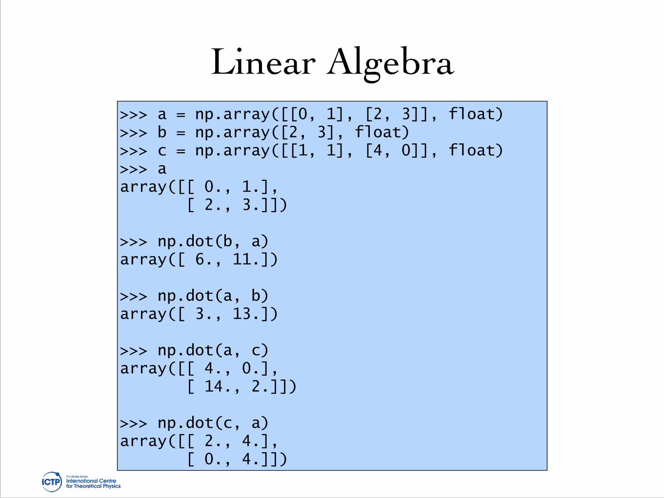
Linear Algebra>>> a = np.array([[0, 1], [2, 3]], float) >>> b = np.array([2, 3], float) >>> c = np.array([[1, 1], [4, 0]], float) >>> a array([[ 0., 1.], [ 2., 3.]]) !>>> np.dot(b, a) array([ 6., 11.]) !>>> np.dot(a, b) array([ 3., 13.]) !>>> np.dot(a, c) array([[ 4., 0.], [ 14., 2.]]) !>>> np.dot(c, a) array([[ 2., 4.], [ 0., 4.]])

Linear Algebra

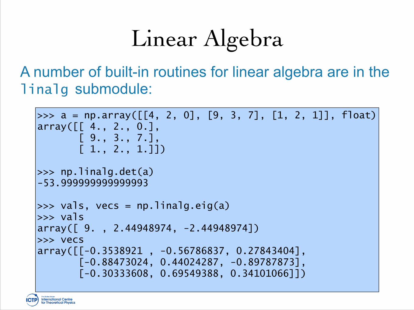
>>> a = np.array([[4, 2, 0], [9, 3, 7], [1, 2, 1]], float) array([[ 4., 2., 0.], [ 9., 3., 7.], [ 1., 2., 1.]]) !>>> np.linalg.det(a) -53.999999999999993 !>>> vals, vecs = np.linalg.eig(a) >>> valsarray([ 9. , 2.44948974, -2.44948974]) >>> vecs array([[-0.3538921 , -0.56786837, 0.27843404], [-0.88473024, 0.44024287, -0.89787873], [-0.30333608, 0.69549388, 0.34101066]])

A number of built-in routines for linear algebra are in the linalg submodule:

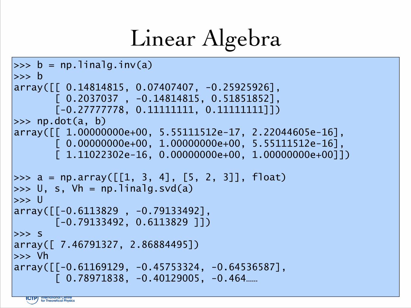
Linear Algebra>>> b = np.linalg.inv(a) >>> barray([[ 0.14814815, 0.07407407, -0.25925926], [ 0.2037037 , -0.14814815, 0.51851852], [-0.27777778, 0.11111111, 0.11111111]]) >>> np.dot(a, b) array([[ 1.00000000e+00, 5.55111512e-17, 2.22044605e-16], [ 0.00000000e+00, 1.00000000e+00, 5.55111512e-16], [ 1.11022302e-16, 0.00000000e+00, 1.00000000e+00]]) !>>> a = np.array([[1, 3, 4], [5, 2, 3]], float) >>> U, s, Vh = np.linalg.svd(a) >>> Uarray([[-0.6113829 , -0.79133492], [-0.79133492, 0.6113829 ]]) >>> s array([ 7.46791327, 2.86884495]) >>> Vharray([[-0.61169129, -0.45753324, -0.64536587], [ 0.78971838, -0.40129005, -0.464……

NumPy offers much more: • Polynomial Mathematics • Statistical computations • Full suite of pseudo-random number generators and operations • Discrete Fourier transforms, • more complex linear algebra operations • size / shape / type testing of arrays, • splitting and joining arrays, histograms • creating arrays of numbers spaced in various ways • creating and evaluating functions on grid arrays • treating arrays with special (NaN, Inf) values • set operations • creating various kinds of special matrices • evaluating special mathematical functions (e.g. Bessel functions) ! • To learn more, consult the NumPy documentation at

http://docs.scipy.org/doc/

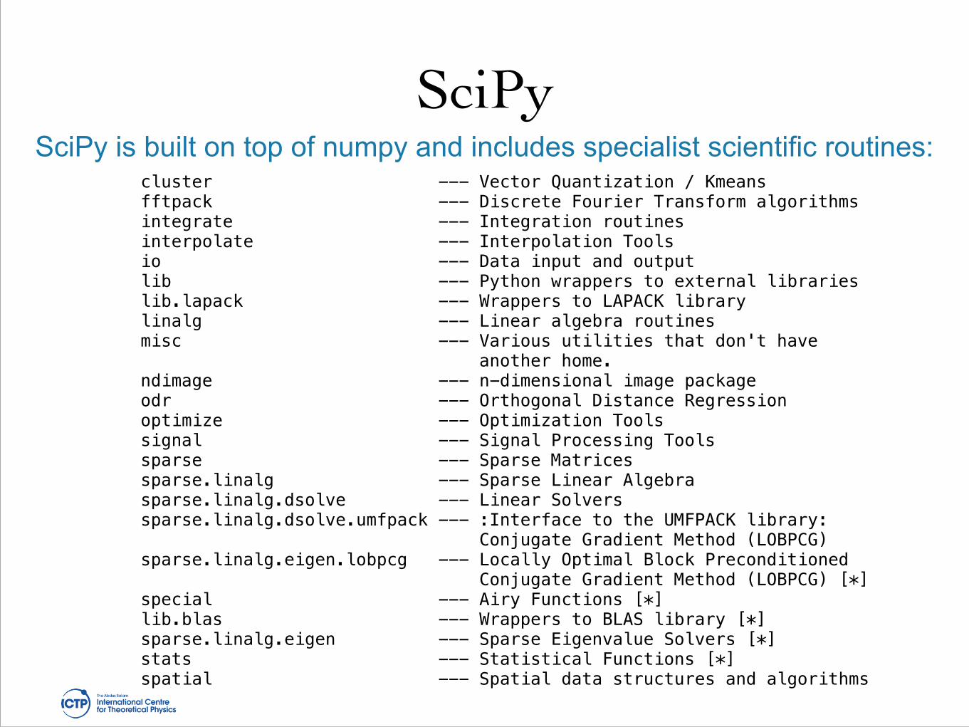
SciPySciPy is built on top of numpy and includes specialist scientific routines:

cluster --- Vector Quantization / Kmeans fftpack --- Discrete Fourier Transform algorithms integrate --- Integration routines interpolate --- Interpolation Tools io --- Data input and output lib --- Python wrappers to external libraries lib.lapack --- Wrappers to LAPACK library linalg --- Linear algebra routines misc --- Various utilities that don't have another home. ndimage --- n-dimensional image package odr --- Orthogonal Distance Regression optimize --- Optimization Tools signal --- Signal Processing Tools sparse --- Sparse Matrices sparse.linalg --- Sparse Linear Algebra sparse.linalg.dsolve --- Linear Solvers sparse.linalg.dsolve.umfpack --- :Interface to the UMFPACK library: Conjugate Gradient Method (LOBPCG) sparse.linalg.eigen.lobpcg --- Locally Optimal Block Preconditioned Conjugate Gradient Method (LOBPCG) [*] special --- Airy Functions [*] lib.blas --- Wrappers to BLAS library [*] sparse.linalg.eigen --- Sparse Eigenvalue Solvers [*] stats --- Statistical Functions [*] spatial --- Spatial data structures and algorithms

MatplotlibPowerful library for 2D data plotting, some 3D capability

Very well designed: common tasks easy, complex tasks possible.

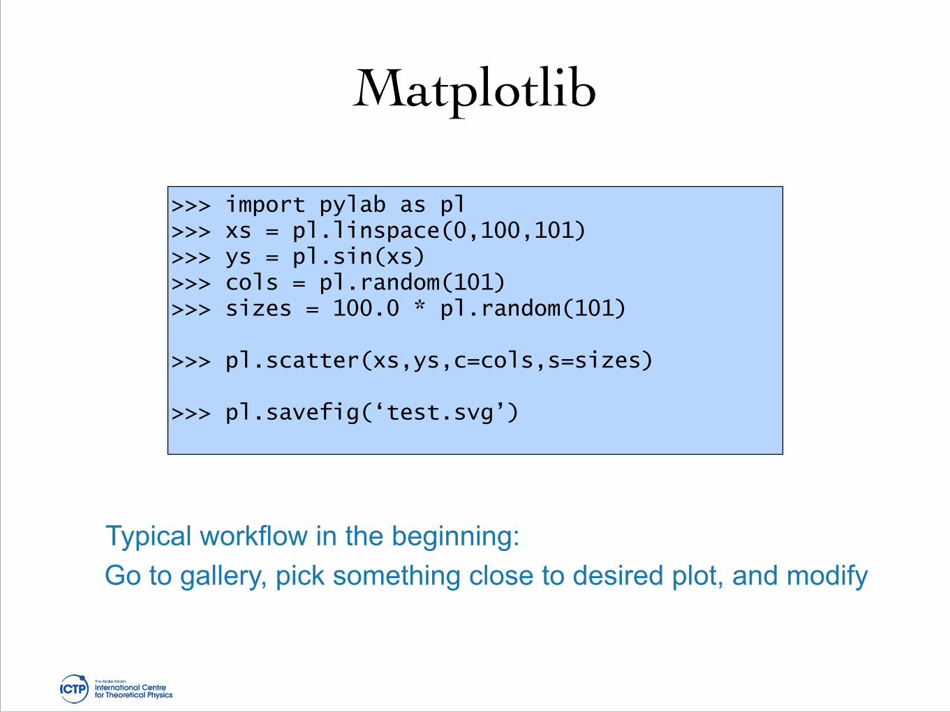
Matplotlib

Typical workflow in the beginning:Go to gallery, pick something close to desired plot, and modify

>>> import pylab as pl >>> xs = pl.linspace(0,100,101) >>> ys = pl.sin(xs) >>> cols = pl.random(101) >>> sizes = 100.0 * pl.random(101) !>>> pl.scatter(xs,ys,c=cols,s=sizes) !>>> pl.savefig(‘test.svg’)

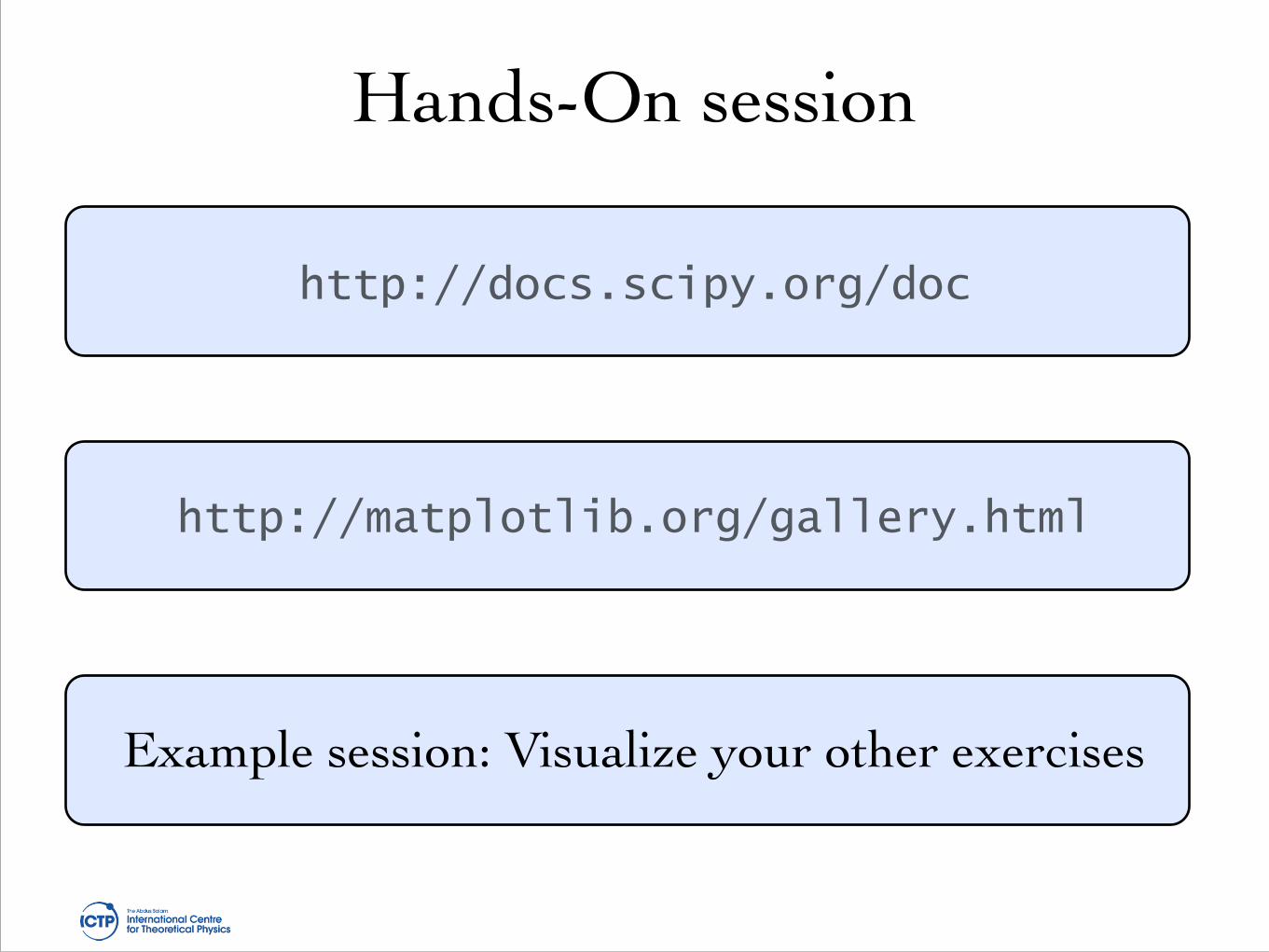
Hands-On session

http://docs.scipy.org/doc

http://matplotlib.org/gallery.html

Example session: Visualize your other exercises