TRANSPORT PROBLEMS 2016 Volume 11 Issue 2 PROBLEMY TRANSPORTU DOI: 10.20858/tp.2016.11.2.1

track alignment; vehicle model; lateral dynamic behaviour;

lateral acceleration; railway dynamics

Mădălina DUMITRIU

University Politehnica of Bucharest 313 Splaiul Independentei, 060042, Bucharest, Romania Corresponding author. E-mail: madalinadumitriu@yahoo.com

NUMERICAL SYNTHESIS OF THE TRACK ALIGNMENT AND APPLICATIONS. PART II: THE SIMULATION OF THE DYNAMIC BEHAVIOUR IN THE RAILWAY VEHICLES

Summary. This paper features a method of synthesizing the track irregularities by which the alignment may be analytically represented by a pseudo-stochastic function, as well as the implementation of such a method in the numerical simulation of the dynamic behaviour of the railway vehicles. The method described in Part I relies on the power spectral density of the track irregularities, as per ORE B 176 and the specifications included in UIC 518 Leaflet regarding the track’s geometric quality. Part II shows the results of the numerical simulations regarding the lateral behaviour of the railway vehicle during the circulation on a tangent track with lateral irregularities, synthesized as in the method herein. These results point out many basic properties of the lateral vibration behaviour of the railway vehicle, a fact that demonstrates the efficiency of the suggested method.

LA SYNTHÈSE NUMERIQUE DU DRESSAGE DE LA VOIE ET APPLICATIONS. PARTIE II: LA SIMULATION DU COMPORTAMENT DYNAMIQUE DANS LES VÉHICULES FERROVIAIRES

Sommaire. L’article présente une méthode pour la synthèse des irrégularités de la voie,

avec laquelle le dressage peut être représenté analytiquement par une fonction pseudo aléatoire et aussi l’application de cette méthode dans la simulation numérique du comportement dynamique latérale des véhicules ferroviaires. La méthode proposée, décrite dans la Partie I de l’article, este basée sur la densité spectrale de puissance des irrégularités de la voie décrite selon ORE B176 et les spécifications contenues dans la Fiche UIC 518 concernant la qualité géométrique de la voie. La Partie II présente les résultats des simulations numériques du le comportement dynamique latéral du véhicule pendant la circulation sur une voie en alignement avec des irrégularités latérales synthétisées en utilisant la méthode présentée. Il met en évidence un certain nombre de propriétés de base du régime de vibrations latérales du véhicule ferroviaires, ce qui démontre l’efficacité de la méthode présentée.

1. INTRODUCTION

The numerical simulations represent basic tools in research, as they are used since the designing stage to estimate the dynamic behaviour of the railway vehicle and the optimization of its dynamic performance and in the investigation of the problems arising during exploitation [1, 2]. In recent years,

6 M. Dumitriu the specifications on the homologation of the railway vehicles, in terms of the dynamic behaviour for safety, track fatigue and ride quality [3, 4], have been added to a series of requirements to complete the tests based on computational models of the vehicle and virtual simulations, thus regulating the so-called virtual homologation procedure [5 - 8]. In comparison with the on-track tests that are expensive, require a considerable investment of time and effort and may be affected by out-of-control series of variables, the numerical simulations have a certain advantage as they allow the examination of the dynamic behaviour of the vehicle, even in the vicinity of extreme circumstances that cannot be marked out during real testing conditions [1].

As a principle, the software applications for simulating the dynamics of the railway vehicles are developed based on models of the vehicle/track system, where the typical inputs are represented by the track geometry irregularities [8]. As shown in Part I, the track irregularities can be obtained by measuring the track geometry or be analytically described by virtue of the power spectral density of the measured irregularities of the track. In terms of the models used to evaluate the dynamic behaviour of the railway vehicles, they need to take into account a series of important factors influencing the vibration behaviour of the railway vehicle [9]. Moreover, if the virtual homologation issue is being raised, its model has to be an accurate representation of all the aspects affecting the dynamic behaviour of the real vehicle [10, 11].

From the perspective of the topic in this paper, the vehicle modelling to study the lateral vibrations is what interests us. The degree of complexity of the model generally depends on the matter being examined—stability, ride quality, the comfort of the passengers—as well as on the precision required from the results. One of the converging problems refers to the vehicle stability. This thing is a consequence of the serious instances, such as vehicle derailment and track damage, which can occur once the stability has been lost when the velocity exceeds the value of the critical speed.

To investigate the stability and the influence of certain parameters of the vehicle upon the critical speed, linear or non-linear models are used, depending on the purpose. These models can be simple, with four or six degrees of freedom [12 - 15], or more elaborate, with between 10 and 14 degrees of freedom [16, 17], or even complex, when the vehicle is modelled via systems with 17-38 such degrees [18 - 22].

In this part of the paper, aiming to simulate the lateral dynamic behaviour of the railway vehicle on a stable running during circulation on a tangent track with lateral irregularities synthesized as per the method in Part I, a non-linear complex model of the vehicle/track system is used, with 21 degrees of freedom. The vehicle is modelled so that it includes all the basic components—carbody, suspended massed of the bogies, wheelsets and their elastic drive system, as well as the suspension elements specific to a passenger car (eg. the dampers of the lateral movement and anti-yaw dampers, the antiroll torsion bar). The nonlinearities of the model derive from the non-linear characteristics of the wheel/rail creep forces, the rail lateral reactions acting on the wheelset when its clearance on the track is consumed and the load transfer between the wheels of each wheelset. Based on the numerical simulations, a series of basic properties of the lateral vibration behaviour of the railway vehicle are pointed out, which proves the efficiency of the method suggested for the synthesis of the track alignment.

2. THE MECHANICAL MODEL OF THE VEHICLE/TRACK SYSTEM

To study the lateral dynamic behaviour of the railway vehicle during circulation on a tangent track with lateral irregularities at velocity V, the model in Fig. 1 and Fig. 2 is considered. It is a four-axle vehicle represented via a 21-degree freedom model, which comprises 7 bodies representing the carbody, the suspended masses of the bogies and the four wheelsets, connected among them via Kelvin-Voigt type systems, by which the elastic and damping elements of the two suspension levels are being modelled.

The vehicle carbody is assimilated to a 3-degree freedom rigid body, with the movements of lateral displacement yc, roll ϕc and yaw αc. The following parameters of the carbody are of interest: distance between the pivots of bogies 2ac, mass mc and the inertia moments around the longitudinal axis Jxc and the vertical axis Jzc. The height of the carbody centre of mass referred to in the plan of the secondary suspension is hc.

Numerical synthesis of the track alignment and applications. Part II 7

Fig. 1. The mechanical model of the vehicle/track system − front view Fig. 1. Le modèle mécanique du système du véhicule/voie – vue frontale

Fig. 2. The mechanical model of the vehicle/track system − top view Fig. 2. Le modèle mécanique du système du véhicule/voie – vue de dessus

8 M. Dumitriu

The bogie is also considered a 3-degree freedom rigid body, namely lateral displacement ybi, roll ϕbi and yaw αbi, with i = 1 or 2. The main parameters of the bogies are the wheelbase 2ab, its mass mb, the inertia moment compared to the longitudinal axis Jxb and the inertia moment referred to the vertical axis Jzb. The bogie centre of mass is at level hb1 to the primary suspension plane and at distance hb2 to the secondary suspension plane.

The wheelsets perform a movement of lateral translation – ywj,(j+1) and a movement of rotation around the vertical axle – yawing αwj,(j+1), where j = 2i – 1, for i = 1, 2, while mentioning that the bogie i has the wheelsets j and j + 1, and a rotation movement around its own axis at the angular velocity Ωwj,(j+1) = V/ro + ωwj,(j+1), where ωwj,(j+1) is the angular sliding velocity of the wheelset referred to as V/ro, and ro is the rolling circle radius when the wheelset occupies the middle position on the track. Similarly, due to the shape of the rolling profiles, the wheelset executes two more movements, one of roll and another one of bounce, that are not independent, but rather the effect of the lateral displacement of the wheel on the track. The wheelset parameters are the mass mo and the inertia moments Jxw, Jyw and Jzw.

The rigidities of the elastic elements of the secondary suspension are noted with kxc, kyc and kzc. To limit the yaw movement, each bogie is fitted with an anti-roll bar whose rigidity is kϕc. On the vertical direction, the secondary suspension of a bogie has two dampers, with the damping constant czc each, while in the lateral direction, it has one damper with a damping constant cyc. The anti-yaw dampers mounted on the lateral sides of the bogies have the damping constant cxc. The lateral base of the secondary suspension is noted with 2bc.

The primary suspension corresponding to a wheelset has the transversal base 2bb and is modelled by three Kelvin-Voigt systems that operate on translation in the longitudinal, transversal and vertical direction. These have the elastic constants kxb, kyb, kzb and the damping constants cxb, cyb and czb.

Fig. 3. The track lateral irregularities against the wheelsets Fig. 3. Irrégularités latérales de la voie et la position des essieux

Against each wheelset, the track lateral irregularities are described by the function ζj,,(j+1)(xj,(j+1)),.dependent on the distance along the track, as such

0)( )1(,)1(, =ζ ++ jjjj x , for xj,,(j+1) ≤ 0; )()( )1(,)1(,)1(, +++ ζ=ζ jjjjjj xx , for xj,,(j+1) > 0, (1)

where, depending on the wheelset position in the vehicle unit, (see. Fig. 3) xj,,j+1 is as below:

xx =1 ; baxx −=2 , for i = 1; caxx 23 −= ; cb aaxx 224 −−= , for i = 2, (2) where the abscissa x is calculated as a function of the moment t and velocity V, x = Vt.

During the circulation on a tangent track, the wheelsets usually follow the trajectory given by the track alignment without the consuming of the clearance on the track. This occurs when the vehicle has a stable behaviour. Under such circumstances, the wheel/rail contact takes place on the rolling surface of the profiles and the contact geometry can be described by linear relations, as for the S78 wheel

Numerical synthesis of the track alignment and applications. Part II 9 profile (used at C.F.R.—the Romanian Railway Tracks) and the UIC 60 rail profile [23]. However, there are exceptional situations, such as the loss of stability or the existence of an isolated defect of a great amplitude, when it is possible to have the consuming of the wheelset clearance on the track and shocks between the wheel flange and the inside rail flank. The modelling of these latter situations is possible by the introduction of a lateral reaction with a non-linear characteristic, which operates upon the outer wheel where the wheelset has consumed the clearance on the track σ [16]. The equation of such force can be given as

⎟⎠⎞⎜

⎝⎛ σ−ζ−ζ−⎟

⎠⎞⎜

⎝⎛ σ−ζ−= +++++++σ 2

)(sign2 1,1,1,1,1,1,1, jjjwjyrjjjwjjjjwjjj ykyyHY , (3)

where kyr is the rail lateral stiffness and H(.) is the Heaviside’s unit step function. 3. THE VEHICLE EQUATIONS OF MOTION

The equations of motion of the vehicle carbody (lateral, roll and yaw) are:

; 0)]()()(2[2

)]()()(2[

21221

21221

=ϕ+ϕ++−ϕ++

+ϕ+ϕ++−ϕ++

bbbbbcccyc

bbbbbcccyccc

hyyhyk

hyyhycym !!!!!!!! (4)

; 0

)]()()(2[2)](2)[2(

)]()()(2[)](2[2

21221212

21221212

=ϕ−

−ϕ+ϕ++−ϕ++ϕ+ϕ−ϕ++

+ϕ+ϕ++−ϕ++ϕ+ϕ−ϕ+ϕ

ϕ

ccc

bbbbbccccycbbcczcc

bbbbbccccycbbcczccxc

ghm

hyyhyhkbkk

hyyhyhcbcJ !!!!!!!!!!!

(5)

.0)]()(2[2)](2[2

)]()(2[)](2[2

21221212

21221212

=ϕ−ϕ+−−α+α+α−α+

+ϕ−ϕ+−−α+α+α−α+α

bbbbbcccycbbccxc

bbbbbcccycbbccxcczc

hyyaakbk

hyyaacbcJ !!!!!!!!!! (6)

For the bogies, the equations of motion of lateral displacement, roll and yaw are given by the equations (7) – (9), for i = 1, 2 and j = 2i – 1:

; 0)]()(2[2])1([2

)]()(2[2])1([

)1(11

2

)1(11

12

=+−ϕ++α−−ϕ−−ϕ−+

++−ϕ++α−−ϕ−−ϕ−+

++

++

jwwjbibbiybcci

cccbibbiyc

jwwjbibbiybcci

cccbbbiycbib

yyhykahyhyk

yyhycahyhycym !!!!!!!!!!!

(7)

;h with , 0)]2/(4[

)]()(2[2])1([2

))(2(4)]()(2[2

])1([)(2

21121122

)1(111

22

22)1(11

122

2

bbbibbcbzb

jwwjbibibbybcci

cccbibibbyc

cbiczccbibzbjwwjbibibbyb

cci

cccbibibbyccbiczcbixb

hhmhmhgbk

yyyhhkahyyhhk

bkkbcyyyhhc

ahyyhhcbcJ

+==ϕ+−+

++−+ϕ+α−+ϕ++−ϕ

+ϕ−ϕ++ϕ++−+ϕ+

+α−+ϕ++−ϕ+ϕ−ϕ+ϕ

++

ϕ+

+

!!!!!

!!!!!!!!!

(8)

.0)](2[2)](2[2

)(2)](2[2

)](2[2)(2

)1()1(2

2)1(

)1(22

=−−α+α+α−α+

+α−α+−−α+

+α+α−α+α−α+α

++

+

+

jwwjbibbybjwwjbibxb

cbicxcjwwjbibbyb

jwwjbibxbcbicxcbizb

yyaakbk

bkyyaac

bcbcJ

!!!

!!!!!!!

(9)

10 M. Dumitriu

For the wheelsets ‘j’, the equations of motion of lateral displacement, and yaw, with i = 1, 2 and j = 2i – 1, are:

jjjbibbibbiwjybbibbibbiwjybwjw YYYahyykahyycym σ−+=α−ϕ−−+α−ϕ−−+ 2111 )(2)(2 !!!!!! ;

(10)

).()/()(2)(2 2122

jjowjoywbiwjbxbbiwjbxbwjzw XXerVJbkbcJ −−=ϕ+α−α+α−α+α !!!!! (11)

)( 21 jjowjyw XXrJ +−=ω! , (12)

where eo, ro – the coordinates of the wheel-rail contact points when the wheelset is in a median position on the track; the term wjoyw rVJ ϕ!)/( corresponds to the gyroscopic moment due to the combined effect of the wheelset rotation motion around its own axis with the roll motion; Xj,(j+1)1,2 are the longitudinal forces and Yj,(j+1)1,2 represent the guidance forces acting upon the wheelsets j and j + 1, respectively, in the wheel/rail contact points 1 or 2.

The above equations are added to the bouncing and roll equations of the wheelsets, motions that are dependent on the lateral displacement of the wheelset on the track. Thus, when considering that the bounce coming from the lateral displacement of the wheelset on the track is very low [24], the inertia effect of the wheelset mass in the vertical direction can be neglected. Hence, the balance equation of the vertical forces can be written as

ojj QQQ 221 =+ , (13)

where Qj,(j+1)1,2 are the vertical loads in the wheel/rail contact points and Qo is the static load on the wheel.

The equation of the wheelset roll motion is as such

jojjojjobizbbbizbbwjoywwjxw YrQQeYYrkbcbrVJJ σ+−++=ϕ−ϕ−α−ϕ )()(22)/( 212122 !!!! ,

(14) where the term 1,)/( +α jwjoyw rVJ ! corresponds to the gyroscopic moment due to the combined effect of the rotation motion of the wheelset around its own axis with the yaw motion.

The wheel/rail contact forces, namely, the longitudinal forces, guidance forces and the vertical loads, are expressed in dependence on the components of the creep forces Tj1,2 and the normal reactions Nj1,2 in the wheel/rail contact points, according to the relations [24]

2,12,1 xjj TX = ; (15)

2,12,12,12,12,1 sincos jjjyjj NTY γγ= ! ; (16)

2,12,12,12,12,1 cossin jjjyjj NTQ γ+γ±= , (17)

where γj1,2 represents the wheel/rail contact angle. To calculate the longitudinal and lateral components Txj and Tyj of the creep force, the relations

corresponding to the Polach non-linear method [25] are applied and the normal reactions on the wheel/rail contact surface are determined by equations (13) and (14). 4. THE SIMULATION OF THE DYNAMIC BEHAVIOUR IN A RAILWAY VEHICLE ON A TRACK WITH LATERAL IRREGULARITIES

This section features the results of the numerical simulations regarding the lateral dynamic

behaviour of the railway vehicle while running on a track whose value of the alignment standards deviation corresponds to the QN2 quality level and to the maximum velocity of 200 km/h. These simulations have the role of showing the efficiency of the method to synthesize the track alignment as in Part I of this paper, for which purpose the model of the vehicle/track system previously described is being used.

Numerical synthesis of the track alignment and applications. Part II 11

Table 1 The parameters of the numerical model

mc = 34000 kg; 2cxc = 50 kNs/m

mb = 3200 kg cyc = 15.205 kNs/m

mw = 1650 kg 2czc = 34.44 kNs/m

2ac = 19 m 2kxc = 340 kN/m

2ab = 2.56 m 2kyc = 340 kN/m

Jxc = 57460 kgm2 2kzc = 1.2 MN/m Jzc = 2456500 kgm2 kϕc = 10 kNm Jxb = 3200 kgm2 4cxb = 100 kNs/m

Jzb = 5000 kgm2 4cyb = 35.77 kNs/m

Jxw = Jzw = 928.125 kgm2 4czb = 52.21 kNs/m

Jyw = 349.14 kgm2 4kxb = 140 MN/m

hc = 1.3 m 4kyb = 10 MN/m

hb1 = 0.25 m 4kzb = 4.4 MN/m

hb2 = 0.2 m kyr = 100 MN/m

2bb = 2bc = 2 m σ = 0.012 m

As for the parameters of the numerical model, they are defined in Tab. 1. Similarly, it should be mentioned that the S78 wear profile wheel and the UIC 60 rail with the standard cant at CFR of 1/20 [24] are taken into account. For the median position of the wheelset on a track with normal gauge, the coordinates of the contact points are ro = 0.4598 m and eo = 0.754 m [23].

Fig. 4 shows the relative wheelset/track displacement for all four wheelsets of the vehicle at the maximum speed of 200 km/h, based on which the nature of the vehicle motion can be evaluated. It is about a stable motion, with maximum lateral wheelset displacements smaller than 6 mm (see Fig. 5) or, in other words, without the wheelset completing the clearance on the track (σ/2). On the other hand, it can be noticed that the front wheelsets of each of the two bogies travel more than the rear ones.

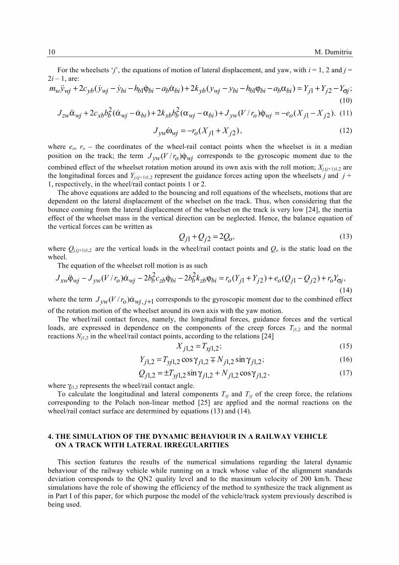
Fig. 6 features the carbody lateral accelerations obtained by the numerical simulation of the time response of the vehicle during the circulation at the speed of 100 km/h [diagrams (a) – (c)], and 200 km/h [diagrams (a’) – (c’)]. These are calculated in three reference points along the carbody longitudinal axis, at the floor level—at the carbody centre and above the two bogies. According to table 2, with the maximum values of the lateral acceleration and its root mean square, the conclusion is that the level of vibrations is lower at the carbody centre than above the bogies. On the other hand, the different vibration behaviours of the carbody should be noticed in the reference points located above the two bogies. Should the carbody critical point in terms of the vibrations level be that reference point where the acceleration is highest, this former point can be shown to be against the rear bogie at the speed of 100 km/h. If the vehicle runs at 200 km/h, the critical point of the carbody is above the first bogie.

12 M. Dumitriu

Fig. 4. Relative lateral wheelset/track displacement at 200 km/h: (a) wheelset 1; (b) wheelset 2; (c) wheelset 3;

(d) wheelset 4 Fig. 4. Déplacement latéral relatif entre l’essieu et voie a 200 km/h: (a) essieu 1; (b) essieu 2; (c) essieu 3;

(d) essieu 4

Fig. 5. Maximum value of relative lateral wheelset/track displacement at 200 km/h Fig. 5. La valeur maximale du déplacement latérale relatif entre l’essieu et voie a 200 km/h

Table 2

The maximum value and the root mean square of the carbody lateral acceleration for QN2 quality level

Speed (km/h) Acceleration (m/s2) At carbody centre Above the front bogie

Above the rear bogie

100 Maximum value 0.29 0.28 0.38 Root mean square 0.08 0.10 0.12

200 Maximum value 0.32 0.40 0.44 Root mean square 0.09 0.14 0.12

Numerical synthesis of the track alignment and applications. Part II 13

Fig. 6. The lateral acceleration of the vehicle carbody: 100 km/h − (a) at the carbody centre, (b) above the front

bogie, (c) above the rear bogie; 200 km/h − (a’) at the carbody centre, (b’) above the front bogie, (c’) above the rear bogie

Fig. 6. L’accélération latérale de la caisse du véhicule: 100 km/h – (a) au milieu de la caisse; (b) au-dessus du premier bogie; (c) au-dessus du deuxième bogie; 200 km/h – (a’) au milieu de la caisse; (b’) au-dessus du premier bogie; (c’) au-dessus du deuxième bogie

Table 3

The maximum value and the root mean square of the carbody lateral acceleration for QN1 quality level

Speed (km/h) Acceleration (m/s2) At carbody centre Above the front bogie

Above the rear bogie

100 Maximum value 0.22 0.23 0.28 Root mean square 0.06 0.07 0.08

200 Maximum value 0.21 0.31 0.25 Root mean square 0.06 0.09 0.08

14 M. Dumitriu

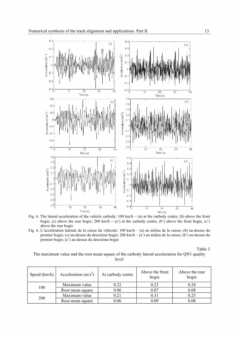
It will be interesting to make a comparison between track with level QN1 and track with level QN2. To this end, table 3 shows the maximum values of the lateral acceleration and its root mean square for a track with level QN1. It observes that main characteristics of the vibration behaviour are the same, and the lateral acceleration is smaller at carbody centre and higher above the bogies. In addition, the position of the critical point remains unchanged. As expected, lateral acceleration decreases when the vehicle runs on a good track (QN1 quality level). For instance, the root mean square of the lateral acceleration decreases with 33-36 % above bogies at 200 km/h.

Fig. 7. The spectra of the carbody lateral acceleration at velocity of 200 km/h: (a) at carbody centre; (b) above

the first bogie; (c) above the rear bogie Fig. 7. Spectres d’accélération latérale de la caisse pendant la circulation a 200 km/h: (a) au milieu de la caisse;

(b) au-dessus du premier bogie; (c) au-dessus du deuxième bogie

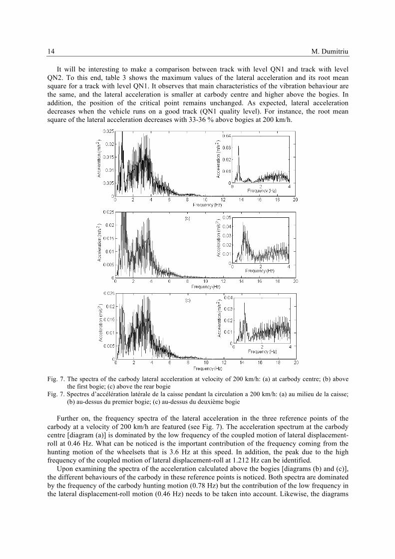
Further on, the frequency spectra of the lateral acceleration in the three reference points of the carbody at a velocity of 200 km/h are featured (see Fig. 7). The acceleration spectrum at the carbody centre [diagram (a)] is dominated by the low frequency of the coupled motion of lateral displacement-roll at 0.46 Hz. What can be noticed is the important contribution of the frequency coming from the hunting motion of the wheelsets that is 3.6 Hz at this speed. In addition, the peak due to the high frequency of the coupled motion of lateral displacement-roll at 1.212 Hz can be identified.

Upon examining the spectra of the acceleration calculated above the bogies [diagrams (b) and (c)], the different behaviours of the carbody in these reference points is noticed. Both spectra are dominated by the frequency of the carbody hunting motion (0.78 Hz) but the contribution of the low frequency in the lateral displacement-roll motion (0.46 Hz) needs to be taken into account. Likewise, the diagrams

Numerical synthesis of the track alignment and applications. Part II 15 of the acceleration spectra above the bogies show the accentuated influence of the hunting motion of the wheelsets. 5. CONCLUSIONS

Part II of the paper has aimed to verify the efficiency of the synthesization method of the track alignment presented in Part I, which was possible by means of the results derived from simulation of the lateral dynamic behaviour of the railway vehicle at sub-critical speeds. For this purpose, the track alignment, synthesized via the suggested method, was implemented into a program of numerical simulation developed on a complex model of the vehicle, which includes a series of elements giving it a non-linear behaviour.

The results presented herein have pointed out at a series of properties specific to the lateral vibrations behaviour of the railway vehicle. Thus, based on the analysis of the time evolution of the carbody lateral acceleration, it has been demonstrated that the level of vibrations is lower at the carbody centre than above the bogies, irrespective of the velocity. Similarly, the different carbody vibrations behaviour in the reference points above the two bogies has been highlighted, as well as the fact that the carbody critical point – in terms of the level of vibrations - can be found either above the front bogie or the rear one, depending on velocity.

On the other hand, the analysis of the frequency spectra of the carbody acceleration has helped identify the resonance frequencies of the lateral motion in the vehicle carbody, namely: the frequencies of the coupled motion of lateral displacement-roll at 0.46 Hz and 1.21 Hz; the frequency of the hunting motion at 0.78 Hz. Similarly, the important contribution of the frequency of the wheelsets hunting motion has been confirmed, which has the value of circa 3.6 Hz at the velocity of 200 km/h.

References

1. Evans, J. & Berg, M. Challenges in simulation of rail vehicle dynamics, Vehicle System Dynamics. 2009. Vol. 47. P. 1023–1048.

2. Schupp, G. Simulation of railway vehicles: Necessities and applications. Mechanics Based Design of Structures and Machines. Vol. 31. I. 3. P. 297–314.

3. UIC 518 Leaflet - 4th edition - Sept. 2009. Testing and approval of railway vehicles from the point of view of their dynamic behaviour – Safety – Track fatigue – Running behaviour.

4. EN 14363 – 2013. Railway applications - Testing and Simulation for the acceptance of running characteristics of railway vehicles - Running behaviour and stationary tests.

5. Funfschilling, C. & Bezin, Y. & Sebès, M. DynoTRAIN: Introduction of simulation in the certification process of railway vehicles. In: Transport Research Arena. Paris, 2014.

6. Funfschilling, C. & Perrin, G. & Kraft, S. Propagation of variability in railway dynamic simulations: Application to virtual homologation. Vehicle System Dynamics. 2012. Vol. 50. Supplement. P. 245–261.

7. Wolter, K.U. & Zacher, M. & Slovak, B. Correlation between track geometry quality and vehicle reactions in the virtual rolling stock homologation process. In: 9th World Congress on Railway Research, May 22-26, 2011.

8. Iwnicki, S. Handbook of railway vehicle dynamics, CRC Press Taylor & Francis Group, 2006. 9. Sebeşan, I. & Mazilu, T. Vibraţiile vehiculelor feroviare. Bucureşti. Ed. MatrixRom. 2010. 486 p.

[In Romanian: Sebeşan, I. & Mazilu, T. Vibrations of the railway vehicles. Bucharest, Ed. MatrixRom].

10. Dumitriu, M. Modeling of railway vehicles for virtual homologation from dynamic behavior perspective. Applied Mechanics and Materials. 2013. Vol. 371. P. 647-651.

11. Mazzola, L. & Alfi, S. & Bruni, S. The influence of modelling of the suspension components on the virtual homologation of a railway vehicle. In: Proceedings of the First International

16 M. Dumitriu

Conference on Railway Technology: Research, Development and Maintenance. Spain, 2012. Civil-Comp Press. Stirlingshire. UK. Paper 75.

12. Wickens, A.H. Static and dynamic instabilities of bogie railway vehicles with linkage steered wheelsets. Vehicle System Dynamics. 1996. Vol. 26. P. 1–16.

13. Piotrowski, J. Stability of freight vehicles with the H-frame 2-axle cross-braced bogies. Simplified theory. Vehicle Systems Dynamics. 1988. Vol. 17. P. 105–125.

14. Narayana, S. & Dukkipati, R.V. & Osman, M.O.M. A comparative study on lateral stability and steady state curving behavior of unconventional rail truck models. Proceedings of IMechE Part F: Journal of Rail and Rapid Transit. 1994. Vol. 208. P. 1–13.

15. Mehdi, A. & Shaopu, Y. Effect of system nonlinearities on locomotive bogie hunting stability. Vehicle System Dynamics. 1998. Vol. 29. P. 366–384.

16. Lee, S.Y. & Cheng, Y.C. Influences of the vertical and the roll motions of frames on the hunting stability of trucks moving on curved tracks. Journal of Sound and Vibration. 2006. Vol. 294. P. 441–453.

17. Park, J.P. & Koh, H.I. & Kim, N.P. Parametric study of lateral stability for a railway vehicle. Journal of Mechanical Science and Technology. 2011. Vol. 25. No. 7. P. 1657-1666.

18. He, Y. & McPhee, J. Optimization of the lateral stability of rail vehicles. Vehicle System Dynamics. 2002. Vol. 38. No. 5. P. 361–390.

19. Dikmen, F. & Bayraktar, M. & Guclu, R. Vibration analysis of 19 degrees of freedom rail vehicle. Scientific Research and Essays. 2011. Vol. 6. No. 26. P. 5600-5608.

20. Zeng, J. & Wu, P. Stability analysis of high speed railway vehicles. JSME International Journal, Series C: Mechanical Systems, Machine Elements and Manufacturing. 2004. Vol. 47. No. 2. P. 464–470.

21. Cheng, Y.C. & Leeb, S.Y. & Chen, H.H. Modeling and nonlinear hunting stability analysis of high-speed railway vehicle moving on curved track. Journal Sound and Vibration. 2009. Vol. 324. P. 139-160.

22. Ranjbar, M. & Ghazavi, M.R. Bifurcation analysis of high-speed railway vehicle in a curve. International Journal on Production and Industrial Engineering. 2013. Vol. 4. No. 1. P. 13-17.

23. Dumitriu, M. Modelling the geometric contact between wheels and the rails of a track with horizontal irregularity. Mechanical Journal Fiability and Durability. 2013. No. 1. P. 116 – 122.

24. Sebeşan, I. Dinamica vehiculelor feroviare. Bucureşti. Ed. MatrixRom. 2011. 526 p. [In Romanian: Sebeşan, I. Dynamic of the railway vehicles. Bucharest, Ed. MatrixRom].

25. Polach, O. A fast wheel–rail forces calculation computer code. Vehicle System Dynamics. 1999. Suppl. 33. P. 728–739.

Received 01.02.2015; accepted in revised form 06.05.2016