American Journal of Computational Mathematics, 2015, 5, 158-174 Published Online June 2015 in SciRes. http://www.scirp.org/journal/ajcm http://dx.doi.org/10.4236/ajcm.2015.52013

How to cite this paper: El-Dabe, N.T., Ghaly, A.Y., Rizkallah, R.R., Ewis, K.M. and Al-Bareda, A.S. (2015) Numerical Solution of MHD Flow of Micropolar Fluid with Heat and Mass Transfer towards a Stagnation Point on a Vertical Plate. American Journal of Computational Mathematics, 5, 158-174. http://dx.doi.org/10.4236/ajcm.2015.52013

Numerical Solution of MHD Flow of Micropolar Fluid with Heat and Mass Transfer towards a Stagnation Point on a Vertical Plate N. T. El-Dabe1, A. Y. Ghaly1, R. R. Rizkallah1, K. M. Ewis2, A. S. Al-Bareda1* 1Department of Mathematics, Faculty of Education, Ain Shams University, Cairo, Egypt 2Department of Engineering Mathematics and Physics, Faculty of Engineering, El-Fayoum University, El-Fayoum, Egypt Email: *ameen_azeez@hotmail.com Received 21 April 2015; accepted 14 June 2015; published 18 June 2015

Copyright © 2015 by authors and Scientific Research Publishing Inc. This work is licensed under the Creative Commons Attribution International License (CC BY). http://creativecommons.org/licenses/by/4.0/

Abstract The paper investigates the numerical solution of problem of magnetohydrodynamic (MHD) mi-cropolar fluid flow with heat and mass transfer towards a stagnation point on a vertical plate. In this study, we consider both strong concentrations (n = 0) and weak concentrations (n = 1/2). The governing equations have been transformed into nonlinear ordinary differential equations by ap-plying the similarity transformation and have been solved numerically by using the finite differ-ence method (FDM) and analytically by using (DTM). The effects of various governing parameters, namely, material parameter, radiation parameter, magnetic parameter, Prandtl number, Schmidt number, chemical reaction parameter and Soret number on the velocity, microrotation, tempera-ture and concentration have been computed and discussed in detail through some figures and tables. In order to verify the accuracy of the present results, we have compared these results with the analytical solutions by using the differential transform method (DTM) and the multi-step dif-ferential transform method (MDTM). It is observed that this approximate numerical solution is in good agreement with the analytical solution.

Keywords Finite Difference Method (FDM), Differential Transform Method (DTM), Micropolar Fluid, MHD, Heat and Mass Transfer, Stagnation Flow, Chemical Reaction, Radiation

*Corresponding author.

N. T. El-Dabe et al.

159

1. Introduction The hydromagnetic stagnation point flows past heated or cooled bodies have attracted many researchers due to their applications in most of the engineering and natural processes. Examples include plasma studies, blood flow problems, MHD generators, and the cooling of an infinite metallic plate in a cooling bath. The classical two di-mensional stagnation point flow on a flat plate first studied by Hiemenz [1] was extended to axisymmetric case by Homann [2]. The problem of two dynamic impinging stagnation flows of two fluids of different densities was investigated by Wang [3] and it was shown that the flow field depends heavily on the ratios of viscosity and density. The influence of an external magnetic field on Hiemenz flow was studied by Ariel [4]. Two dimension-al MHD steady stagnation point flow towards a stretching surface was analyzed by Mahapatra and Gupta [5]. Ishak et al. [6] theoretically studied the similarity solutions for the steady magnetohydrodynamic flow towards a stagnation point on a vertical surface immersed in an incompressible micropolar fluid. Lokendra Kumar [7] has analyzed the effect of MHD flow of micropolar fluid towards a stagnation point on a vertical stretching sheet. Ishak et al. [8] investigated the steady two-dimensional stagnation point flow of an incompressible micropolar fluid towards a vertical stretching sheet.

The theory of micropolar fluids which is originally formulated by Eringen [9] can be used to explain the flow of crystals, animal blood, paints, polymers, etc. The theory introduces new material parameters, an additional in dependent vector field the microrotation—and new constitutive equations which must be solved simultaneously with the usual equations for Newtonian flow. Ramachandran et al. [10] studied laminar mixed convection in two-dimensional stag nation flows around surfaces. He considered both cases of an arbitrary wall temperature and arbitrary surface heat flux variations and found that they are versed flow developed in the buoyancy oppos-ing flow region, and dual solutions are found to certain range of the buoyancy parameter. Hassanien et al. [11] extended Ramachandran’s work to micropolar fluid. They considered both assisting and opposing flows, but the existence of dual solutions was not reported [12]. Devi et al. extended the problem posed by Ramachandran et al. [10] to the unsteady case, and they found that dual solution exists for a certain range of the buoyancy parameter when the flow is opposing. Similar problem for steady and unsteady cases, for a vertical surface immersed in a micropolar fluid was investigated by Lok et al. [13] [14]. Existence of dual solutions was reported in [13] only for the opposing flow regime. Mahapatra et al. [15] examined heat transfer in stagnation-point flow on stret-ching sheet with viscous dissipation effect. Attia [16] studied the hydromagnetic stagnation point flow on porous stretching sheet with suction and injection. El-dabe et al. [17] studied the peristaltic motion of incompressible micropolar fluid through a porous medium in a two-dimensional channel under the effects of heat absorption and chemical reaction in the presence of magnetic field. Effects of thermal radiation on magnetohydrodynamic (MHD) flow of a micropolar fluid towards a stagnation point on a vertical Plate were studied by Olanrewaju et al. [18]. Pop et al. [19] examined the flow over a stretching sheet near a stagnation point taking radiation effect. Olanrewaju and Adesanya [20] studied the effects of radiation and viscous dissipation on stagnation flow of a micropolar fluid towards a vertical permeable surface. Manjoolatha et al. [21] studied the radiation and mass transfer effects on MHD flow of a micropolar fluid towards a stagnation point on a vertical stretching sheet.

The main objective of the present work is to study the numerical solutions of problem of magnetohydrody-namic (MHD) micropolar fluid flow with heat and mass transfer towards a stagnation point on a vertical plate. In this study, we consider both strong concentrations (n = 0) and weak concentrations (n = 1/2). The governing equations have been transformed into nonlinear ordinary differential equations by applying the similarity trans-formation and have been solved numerically by using the finite difference method (FDM) and analytically by using (DTM). The effects of various parameters of the problem on fluid velocity, microrotation, temperature and concentration have been computed and discussed in detail through some figures and tables. Comparisons with analytical solution by using (DTM) of present work are performed and show that the present results apply with results of analytical solution, as well as the comparisons with previous published results and are found to be in good agreement.

2. Mathematical Formulation We consider the steady, two-dimensional flow of an incompressible electrically conducting micropolar fluid near the stagnation point on a vertical heated stretching sheet placed in the (y = 0) of a cartesian coordinate sys-tem with the x-axis along the sheet as shown in Figure 1. The fluid occupies the half plane (y > 0). It is assumed

N. T. El-Dabe et al.

160

that the velocity of the flow external to the boundary layer U, the temperature of the sheet wT and concentration of sheet wC are proportional to the distance x from the stagnation point, i.e.

, andw wU ax T T bx C C cx∞ ∞= = + = + where a, b and c are positive constants, wT T∞> with T∞ being the uniform temperature of the fluid and wC C∞> with C∞ being the uniform concentration of the fluid. A uni-form magnetic field of strength 0B is assumed to be applied in the positive y-direction normal to the plate. The magnetic Reynolds number of the flow is taken to be small enough so that the induced magnetic field is negligi-ble.

Under the usual boundary layer approximation, the governing equations are given as follows:

0,u vx y∂ ∂

+ =∂ ∂

(1)

( ) ( ) ( )22

*02

dd

Bu u U k u k Nu v U U u g T T g C Cx y x yy

σµ β βρ ρ ρ ∞ ∞

∂ ∂ + ∂ ∂+ = + + + − ± − ± − ∂ ∂ ∂∂

(2)

2

2 2N N u uj u v k Nx y yy

ρ γ ∂ ∂ ∂ ∂

+ = − + ∂ ∂ ∂∂ (3)

22 2

2 2

1 m Tr

p p s p

D kqT T T u Cu vx y c y c y c cy y

ναρ

∂∂ ∂ ∂ ∂ ∂+ = + − + ∂ ∂ ∂ ∂∂ ∂

(4)

( )2 2

2 2m T

m rm

D kC C C Tu v D K C Cx y Ty y∞

∂ ∂ ∂ ∂+ = − − + ∂ ∂ ∂ ∂

(5)

The boundary conditions are as follows:

( )

0, 0, , , , at 0

, 0, , as

w wuu v N n T T C C yy

u U x N T T C C y∞ ∞

∂= = = − = = =

∂

→ → → → →∞ (6)

where u and v are the velocity components along the x and y direction, g is the acceleration due to gravity, T is the fluid temperature, wT is the plate temperature, T∞ is the ambient temperature, C is the fluid concentration in the boundary layer, wC is the plate concentration, C∞ is the ambient fluid concentration, ν is the kine-

Figure 1. Physical model and coordinate system.

N. T. El-Dabe et al.

161

matic viscosity of the fluid, β is the thermal expansion coefficient, *β is the coefficient of expansion with concentration, 0B is the magnetic field of constant strength, σ is the electric conductivity of the fluid, rq is the radiative heat flux, pc is the specific heat at constant pressure of the fluid, mD is the mass diffusion coef-ficient, mT is the mean fluid temperature, Tk is the thermal diffusivity ratio, sc is concentration susceptibility, and rk is the chemical reaction coefficient. Furthermore, , , , , , andk j Nµ ρ γ α are respectively the dynamic viscosity, vortex viscosity (or the microrotationviscosity), fluid density, microinertia density, microrotation vec-tor (or angular velocity), spingradient viscosity and thermal diffusivity.

We follow the work of many authors by assuming that 12 2k Kjγ µ µ = + = +

where

kKµ

= is the

material parameter. This assumption is involved to allow the field of equations predicts the correct behavior in the limiting case when the microstructure effects become negligible and the total spin N reduces to the angular velocity (see Ishak et al. [6]).

By using the Rosseland approximation (Brewster [22]), the radiative heat flux rq is given by given by * 4

*

43r

Tqyk

σ ∂= −

∂ (7)

where *σ is the Stefan-Boltzmann constant and *k is the mean absorption coefficient. It should be noted that by using the Rosseland approximation, the present analysis is limited to optically thick fluids. If temperature differences within the flow are sufficiently small, then Equation (7) can be linearized by expanding 4T into the Taylor series about T∞ , which after neglecting higher order terms takes the form

4 3 44 3T T T T∞ ∞≈ − (8)

In view of Equations (7) and (8), Equation (4) reduces to 2* 3 2 2

* 2 2

161

3m T

p s p

D kTT T T u Cu vx y c y c ckk y y

σ να ∞ ∂ ∂ ∂ ∂ ∂+ = + + + ∂ ∂ ∂∂ ∂

(9)

where k is the constant thermal conductivity.

3. Method of Solutions

To solve system of Equations (1)-(5), we will consider the following similarity transformations:

( ) ( )

( )( )

( )( )

, ,

, , ,w w

a Ny f Na x aax

T T C Cj

a T T C C

ϕη η ην ν

νν θ ∞ ∞

∞ ∞

= = =

− −= = ∅ =

− −

(10)

where η is the independent similarity variable, ( )f η the dimensionless stream function, ( )h η the dimen-sionless micorotation, ( )θ η the dimensionless temperature and ( )η∅ the dimensionless concentration. Fur-ther, ϕ is the stream function which is defined in the usual way

( ) ( ),u Uf v av fη η′= = − (11)

where prime denotes differentiation with respect to η . By using Equation (10) in the Equations (1)-(5) and (9), we get the following ordinary differential equations

in dimensionless form:

( ) ( )21 1 1 0K f ff f Kh M f θ δ′′′ ′′ ′ ′ ′+ + + − + + − ± ± ∅ = (12)

( )1 2 02K h fh f h K h f ′′ ′ ′ ′′+ + − − + =

(13)

N. T. El-Dabe et al.

162

241 03 a r r r r uR P f P f P Ef P Dθ θ θ ′′ ′ ′ ′′ ′′+ + − + + ∅ =

(14)

0 0c c c r cS f S f S K S S θ′′ ′ ′ ′′∅ + ∅ − ∅− ∅+ = (15)

where 20B

Maσρ

= is the magnetic parameter,

2r

ex

GR

= ±

is the thermal buoyancy parameter, ( )± sign has the

same meaning as in Equation (2). For 0 < ג, buoyancy forces act in the direction of the mainstream and fluid is accelerated in the manner of a favorable pressure gradient (assisting flow). When 0 > ג, buoyancy forces oppose the motion, retarding the fluid in the boundary layer, acting as an adverse pressure gradient (opposing flow),

2m

ex

GR

δ = ± is the solutal buoyancy parameter, ( )

2w

r

g T TG

vβ ∞−

= is the local thermal Grashof number,

( )*

2w

m

g C CG

vβ ∞−

= is the local soutal Groshof number, exUxRv

= is the local Reynolds number,

( )2

p w

UEc T T∞

=−

is the Eckert number, Pr

cPk

νρ= is the Prandtl number,

3

*

4a

TRkkσ ∞= , is the radiation para-

meter, cm

SDν

= is the Schmidt number, rr

kKa

= is the Chemical reaction parameter,

( )( )

m T wm Tu

s p s p w

D k C CD k cxD

vc c bx vc c T T∞

∞

−= =

− is the Dufour number and

( )( )0

m T wm T

m m w

D k T TD k bxS

vT cx vT C C∞

∞

−= =

− is the Soret num-

ber. Also, the subjected boundary conditions Equation (6) will now take the form:

( ) ( ) ( ) ( ) ( ) ( )( ) ( ) ( ) ( )0 0, 0 0, 0 0 , 0 1, 0 1,

1, 0, 0, 0

f f h nf

f h

θ

θ

′ ′′= = = − = ∅ =

′ ∞ → ∞ → ∞ → ∅ ∞ → (16)

The skin-friction coefficient fC , local Nusselt number uxN and Sherwood number hxS are defined as:

( ) ( )2 , , ,w w wf ux hx

w w

xq xjC N S

k T T D C CUτρ ∞ ∞

= = =− −

(17)

In which , ,w w wq jτ are given by

( )0 00

, , ,w w wy yy

u T Ck q k j Dy y y

τ µ= ==

∂ ∂ ∂= + = − = − ∂ ∂ ∂

(18)

Substituting by similarity transformations and Equation (18) into Equation (17), we get

( ) ( ) ( )1

1 2 1 2 21 0 , 0 , 02f ex ux ex hx exKC R f N R S Rθ

−− ′′ ′ ′= + = − = ∅

(19)

3.1. The Differential Transform Method The differential transformation of an analytical function ( )f t for one variable is defined as [23].

( ) ( )

0

d1! d

k

kt t

f tF k

k t=

= (20)

where f(t) is the original function and F(k) is the transformed function. The differential inverse transformation of F(k) is defined as:

( ) ( )( )00k

kf t F k t t∞

== −∑ (21)

Combining Equations (20) and (21), we obtain

N. T. El-Dabe et al.

163

( ) ( ) ( )

0

00

d! d

k k

kkt t

t t f tf t

k t∞

==

−=

∑ (22)

From Equations (20)-(22), it can be seen that the differential transformation method is derived from Taylor's series expansion, but the method does not calculate the derivatives representatively. However, the relative deriv-atives are calculated by an iterative way which is described by the transformed equations of the original function. For implementation purposes, the function f(t) is expressed by a finite series and Equation (21) can be written as

( ) ( )( )00kN

kf t F k t t=

≈ −∑ (23)

By Equation (20), the following theorems can be deduced: Theorem 1. If ( ) ( ) ( )f t u t v t= ± then ( ) ( ) ( ).F k U k V k= ±

Theorem 2. If ( ) ( )f t u tα= then ( ) ( ).F k U kα=

Theorem 3. If ( ) mf t t= then

( ) ( )1

.0 otherwise

k mF k k mδ

== − =

Theorem 4. If ( ) ( )ddu t

f tt

= then ( ) ( ) ( )1 1 .F k k U k= + +

Theorem 5. If ( ) ( )dd

n

n

u tf t

t= then ( ) ( ) ( )

!.

!k n

F k U k nk+

= +

Theorem 6. If ( ) ( ) ( )f t u t v t= ⋅ then ( ) ( ) ( )0 .krF k U r V k r=

= −∑

Theorem 7. If ( ) ( ) ( )d dd du t u t

f tt t

= then ( ) ( )( ) ( ) ( )0 1 1 1 1 .krF k r k r U r U k r=

= + − + + − +∑

3.2. Basic Concepts of the Multi-Step Differential Transform Method (MDTM)

When the DTM is used for solving differential equations with the boundary condition at infinity or problems that have highly non-linear behavior, the obtained results were found to be incorrect (when the boundary-layer variable go to infinity, the obtained series solutions are divergent). Besides that, power series are not useful for large values of the independent variable.

To overcome this shortcoming, the MDTM that has been developed for the analytical solution of the differen-tial equations is presented in this section. For this purpose, the following non-linear initial-value problem is con-sidered:

( )( ), , , , 0pu t f f f′ =

(24)

subject to the initial conditions ( ) ( )0kkf c= , for 0,1, 2, , 1k p= − .

Let [0, T] be the interval over which we want to find the solution of the initial-value problem (24). In actual applications of the DTM, the approximate solution of the initial value problem (24) can be expressed by the fol-lowing finite series:

( ) ( ) [ ]00 , 0,nNnnf t a t t t T

== − ∈∑ (25)

The multi-step approach introduces a new idea for constructing the approximate solution. Assume that the in-terval [0, T] is divided into M subintervals [ ]1,m mt t− , 0,1, 2, ,m M=

of equal step size h = (T/M) by using the nodes tm = mh. The main ideas of the MDTM are as follows. First, we apply the DTM to Equation (24) over the interval [0, t1], we will obtain the following approximate solution:

( ) ( ) [ ]1 1 0 10 , 0,nNnnf t a t t t t

== − ∈∑ (26)

using the initial conditions ( ) ( )1 0 kkf c= . For 2m ≥ and at each subinterval [ ]1,m mt t− we will use the initial

N. T. El-Dabe et al.

164

conditions ( ) ( ) ( ) ( )1 1 1k

mk

m m mf t f t− − −= and apply the DTM to Equation (23) over the interval [ ]1,m mt t− , where 0t in Equation (24) is replaced by 1mt − . The process is repeated and generates a sequence of approximate solutions

( ) 1,2, , ,mf t m M= , for the solution f(t):

( ) ( )[ ]

10

1

,

,

nNm mn mn

m m

f t a t t

t t t−=

−

= −

∈

∑ (27)

where N K M= ⋅ . In fact, the MDTM assumes the following solution:

( )

( ) [ ]( ) [ ]

( ) [ ]

1 1

2 1 2

1

, 0,

, ,

, ,M M M

f t t t

f t t t tf t

f t t t t−

∈

∈= ∈

(28)

The new algorithm, MDTM, is simple for computational performance for all values of h. It is easily observed that if the step size h = T, then the MDTM reduces to the classical DTM. As we will see in the next section, the main advantage of the new algorithm is that the obtained series solution converges for wide time regions and can approximate non-chaotic or chaotic solutions.

3.3. Analytical Solution Be the MDTM By applying the MDTM to Equations (12)-(15), the following recursive relations in each sub-domain ( )1,i it t + ,

0,1, , 1i N= − is given.

(29)

( )( ) [ ] ( ) [ ] [ ]

( ) [ ] [ ] [ ] ( )( ) [ ]( )0

0

1 1 2 2 1 12

1 1 2 1 2 2 0

k

rk

r

K k k H k k r F r H k r

r F r H k r K H k k k F k

=

=

+ + + + + − + − +

− + + − − + + + + =

∑

∑ (30)

( )( ) [ ] ( ) [ ] [ ]

( )( )( )( ) [ ] [ ]

( ) [ ] [ ] ( )( ) [ ]

0

0

0

41 1 2 2 1 13

2 1 2 1 2 2

1 1 1 2 2 0

k

a rr

k

rr

k

r r ur

R k k k P k r F r k r

P E r r k r k r F r F k r

P r F r k r P D k k k

θ θ

θ

=

=

=

+ + + + + − + − +

+ + + − + − + + − +

− + + − + + + ∅ + =

∑

∑

∑

(31)

( )( ) [ ] ( ) [ ] [ ] [ ]

( ) [ ] [ ] ( )( ) [ ]0

0

1 2 2 1 1

1 1 1 2 2 0

k

c c rr

k

c c or

k k k S k r F r k r S K k

S r F r k r S S k k kθ

=

=

+ + ∅ + + − + ∅ − + − ∅

− + + ∅ − + + + + =

∑

∑ (32)

where [ ] [ ] [ ] [ ], , andF k H k k kθ ∅ are the differential transform of ( ) ( ) ( ) ( ), , and .f hη η θ η η∅ The differential transformed boundary conditions in Equation (16) to:

( )( )( )( ) [ ] ( )( ) [ ] [ ]

[ ] ( )( ) [ ] [ ] ( ) [ ]

[ ] ( ) [ ]( ) [ ] [ ]

0

0

1 K 1 2 3 3 1 2 2

1 1 1 1 1 1

1 1 0

k

rk

r

k k k F k k r k r F r F k r

k r k r F r F k r K k H k

M k k F k k k

δ

δ θ δ

=

=

+ + + + + + − + − + − +

+ − + − + + − + + + +

+ − + + ± ± ∅ =

∑

∑

N. T. El-Dabe et al.

165

[ ] [ ] [ ] [ ][ ] [ ] [ ][ ] [ ] [ ]

1 2

1 1 1

0 0, 0 2 , 0 1,

0 1, 1 , 2 ,

1 , 1 , 1 .

F H nF

F f F f

H h t c

θ

θ

= = − =

∅ = = =

= = ∅ =

(33)

where 1 2 1 1 1, , , ,f f h t c are constants. These constants are computed from the boundary condition. Moreover, substituting Equation (33) into Equations (29)-(32) and by using the recursive method, we can

calculate other values of ( ) ( ) ( ) ( ), , andF k H k k kθ ∅ .

Hence, substituting all ( ) ( ) ( ), ( ), andF k H k k kθ ∅ , into Equation (23), we obtain series solutions. The velocity, microrotation, temperature and concentration distributes achieved with the aid of MATHAMATICA

application software.

3.4. Numerical Solution The governing ordinary differential Equations (10)-(12) are being highly nonlinear and difficult to solve analyt-ically. To solve these coupled equations, we use a finite difference based numerical algorithm. Following Ashraf et al. [24], we reduce the order of Equation (12) by one with the help of the substitution:

dd

fq fη

′= = (34)

Equations (12)-(15) in view of Equation (34) can be written as:

( ) ( )21 1 1 0K q fq q Kh M q θ δ′′ ′ ′+ + + − + + − ± ± ∅ = (35)

1 2 02K h fh qh Kh Kq ′′ ′ ′+ + − − − =

(36)

241 03 a r r r r uR P f P q P Eq P Dθ θ θ ′′ ′ ′ ′′+ + − + + ∅ =

(37)

0c c c r c oS f S q S K S S θ′′ ′ ′′∅ + ∅ − ∅− ∅+ = (38)

The boundary conditions:

( ) ( ) ( ) ( ) ( ) ( )( ) ( ) ( ) ( )

0 0, 0 0, 0 0 , 0 1, 0 1,

1, 0, 0 0, 0.

f q h nq

q h

θ

θ

′= = = − = ∅ =

∞ → ∞ → = ∅ ∞ = (39)

Now, we can write Equations (35)-(38) in the following finite difference method form:

( )

( )( )21 1 1 1 1 1

2

21 1 1 0

2 2i i i i i i i

i i i i iq q q q q h h

K f q K M q θ δη ηη

+ − + − + − − + − − + + + − + + − ± ± ∅ = ∆ ∆∆

(40)

( )1 1 1 1 1 1

2

21 2 0

2 2 2i i i i i i i

i i i ih h h h h q qK f q h Kh K

η ηη+ − + − + −

− + − − + + − − + = ∆ ∆ ∆ (41)

( ) ( )

21 1 1 1 1 1 1 1

2 2

2 241 03 2 2

i i i i i i i i i ia r i r i i r r u

q qR P f P q P E P D

θ θ θ θ θθ

η ηη η+ − + − + − + −

− + − − ∅ − ∅ +∅ + + − + + = ∆ ∆ ∆ ∆ (42)

( ) ( )1 1 1 1 1 1

2 2

2 20

2i i i i i i i i

c i c i i c r i c oS f S q S K S Sθ θ θ

ηη η+ − + − + −

∅ − ∅ +∅ ∅ −∅ − + + − ∅ − ∅ + = ∆∆ ∆ (43)

The velocity, microrotation, temperature and concentration distributes at all interior nodal points computed by successive applications of the above finite difference equations and these are achieved with the aid of MATLAB application software.

N. T. El-Dabe et al.

166

4. Results and Discussion In this section, we present our results in tabular and graphical form is shown in Figures 2-16 to illustrate the in-fluence of physical parameters such as, material parameter K, magnetic parameter M, thermal buoyancy ג, so-lutal buoyancy parameter δ , radiation parameter aR , Prandtl number rP , Dufour number uD , Schmidt-number cS , chemical reaction rK and Soret number oS , on the velocity, microrotation, temperature and con-centration when n = 0 and n = 1/2 for both the cases of assisting and opposing flows.

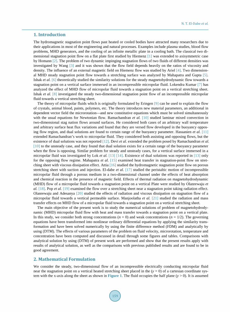
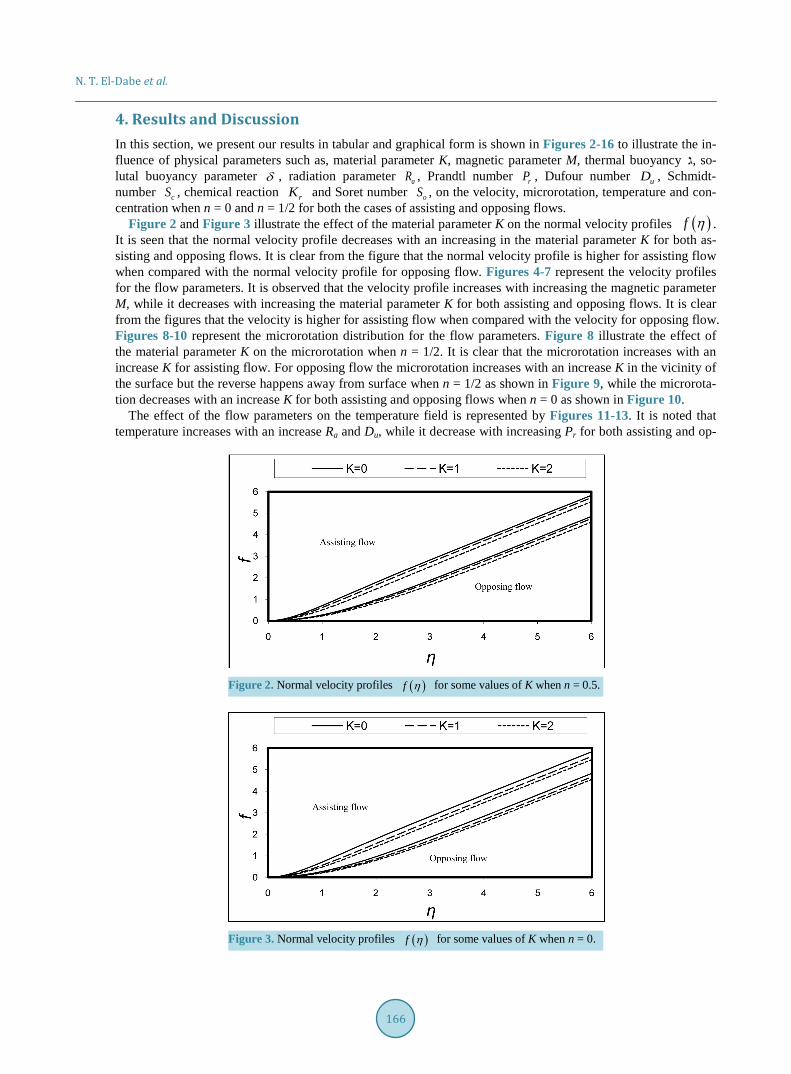
Figure 2 and Figure 3 illustrate the effect of the material parameter K on the normal velocity profiles ( )f η . It is seen that the normal velocity profile decreases with an increasing in the material parameter K for both as-sisting and opposing flows. It is clear from the figure that the normal velocity profile is higher for assisting flow when compared with the normal velocity profile for opposing flow. Figures 4-7 represent the velocity profiles for the flow parameters. It is observed that the velocity profile increases with increasing the magnetic parameter M, while it decreases with increasing the material parameter K for both assisting and opposing flows. It is clear from the figures that the velocity is higher for assisting flow when compared with the velocity for opposing flow. Figures 8-10 represent the microrotation distribution for the flow parameters. Figure 8 illustrate the effect of the material parameter K on the microrotation when n = 1/2. It is clear that the microrotation increases with an increase K for assisting flow. For opposing flow the microrotation increases with an increase K in the vicinity of the surface but the reverse happens away from surface when n = 1/2 as shown in Figure 9, while the microrota-tion decreases with an increase K for both assisting and opposing flows when n = 0 as shown in Figure 10.

The effect of the flow parameters on the temperature field is represented by Figures 11-13. It is noted that temperature increases with an increase Ra and Du, while it decrease with increasing Pr for both assisting and op-

Figure 2. Normal velocity profiles ( )f η for some values of K when n = 0.5.

Figure 3. Normal velocity profiles ( )f η for some values of K when n = 0.

N. T. El-Dabe et al.

167

Figure 4. Velocity profiles ( )f η′ for some values of M when n = 0.5.

Figure 5. Velocity profiles ( )f η′ for some values of M when n = 0.

Figure 6. Velocity profiles ( )f η for some values of K when n = 0.5.

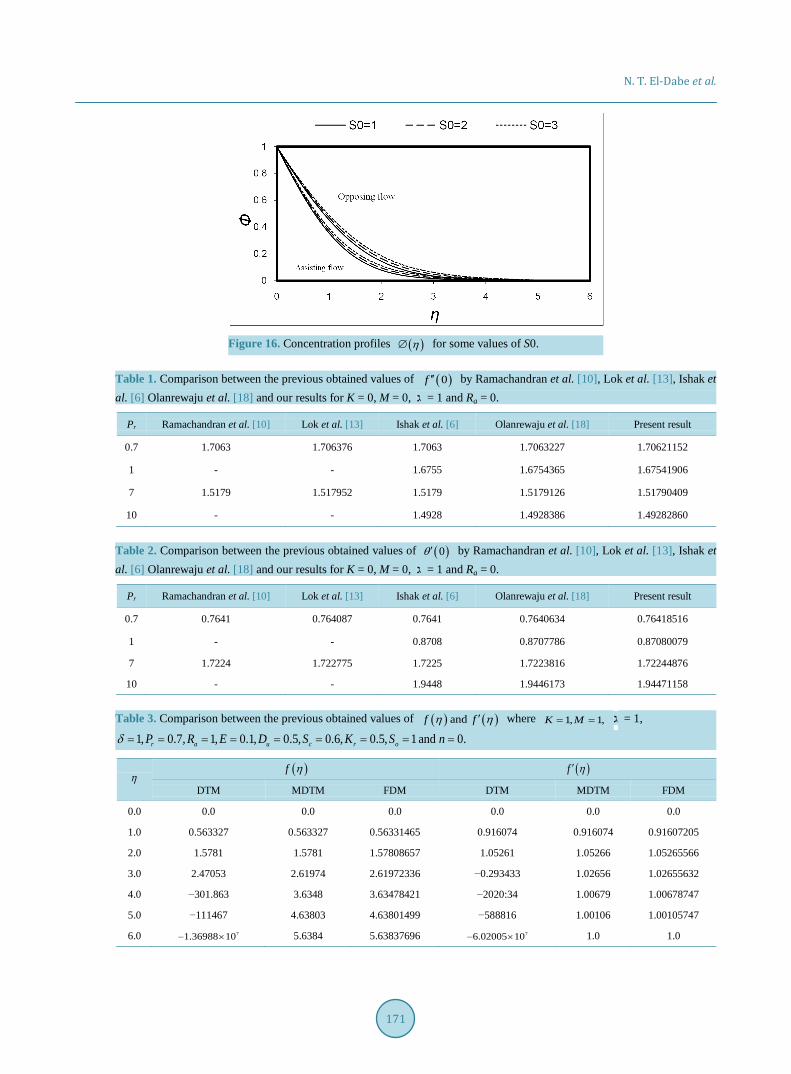
posing flows. It is clear from the figures that the temperature is higher for opposing flow when compared with the temperature for assisting flow. Figures 14-16 represent the concentration profiles for the flow parameters. It is noted that concentration increases with an increases S0, while it decrease with the increases Sc and Kr for both assisting and opposing flows. It is clear from the figures that the concentration is higher for opposing flow when

N. T. El-Dabe et al.

168

Figure 7. Velocity profiles ( )f η for some values of K when n = 0.

Figure 8. Angular velocity profiles ( )h η for some values of K when n = 0.5.

Figure 9. Angular velocity profiles ( )h η for some values of K when n = 0.5.

compared with the concentration for assisting flow.

In order to verify the accuracy of the numerical solution of present work by using (FDM) we have compared

N. T. El-Dabe et al.

169

Figure 10. Angular velocity profiles ( )h η for some values of K when n = 0.

Figure 11. Temperature profiles ( )θ η for some values of Pr.

Figure 12. Temperature profiles ( )θ η for some values of Ra.

these results for ( ) ( )0 and 0 when 1 2f nθ′′ − = with Ramachandran et al. [10], Lok et al. [13], Ishak et al. [6] and Olanrewaju et al. [18]. It is observed that this numerical solution in excellent agreement with the results previous obtained values as shown in Table 1 and Table 2.

Finally, Tables 3-5 show comparison between numerical solution by using (FDM) and the analytical solu-

N. T. El-Dabe et al.

170

Figure 13. Temperature profiles ( )θ η for some values of Du.

Figure 14. Concentration profiles ( )η∅ for some values of Sc.

Figure 15. Concentration profiles ( )η∅ for some values of Kr.

tion using (DTM). It is observed that this approximate numerical solution is in excellent agreement with the re-sults of the analytical solution of by using (DTM).

N. T. El-Dabe et al.

171

Figure 16. Concentration profiles ( )η∅ for some values of S0.

Table 1. Comparison between the previous obtained values of ( )0f ′′ by Ramachandran et al. [10], Lok et al. [13], Ishak et al. [6] Olanrewaju et al. [18] and our results for K = 0, M = 0, 1 = ג and Ra = 0.

Pr Ramachandran et al. [10] Lok et al. [13] Ishak et al. [6] Olanrewaju et al. [18] Present result

0.7 1.7063 1.706376 1.7063 1.7063227 1.70621152

1 - - 1.6755 1.6754365 1.67541906

7 1.5179 1.517952 1.5179 1.5179126 1.51790409

10 - - 1.4928 1.4928386 1.49282860

Table 2. Comparison between the previous obtained values of ( )0θ′ by Ramachandran et al. [10], Lok et al. [13], Ishak et al. [6] Olanrewaju et al. [18] and our results for K = 0, M = 0, 1 = ג and Ra = 0.

Pr Ramachandran et al. [10] Lok et al. [13] Ishak et al. [6] Olanrewaju et al. [18] Present result

0.7 0.7641 0.764087 0.7641 0.7640634 0.76418516

1 - - 0.8708 0.8707786 0.87080079

7 1.7224 1.722775 1.7225 1.7223816 1.72244876

10 - - 1.9448 1.9446173 1.94471158

Table 3. Comparison between the previous obtained values of ( ) ( )andf fη η′ where 1, 1,K M= = ,1 = ג

1, 0.7, 1, 0.1, 0.5, 0.6, 0.5, 1 and 0.r a u c r oP R E D S K S nδ = = = = = = = = =

η ( )f η ( )f η′

DTM MDTM FDM DTM MDTM FDM

0.0 0.0 0.0 0.0 0.0 0.0 0.0

1.0 0.563327 0.563327 0.56331465 0.916074 0.916074 0.91607205

2.0 1.5781 1.5781 1.57808657 1.05261 1.05266 1.05265566

3.0 2.47053 2.61974 2.61972336 −0.293433 1.02656 1.02655632

4.0 −301.863 3.6348 3.63478421 −2020:34 1.00679 1.00678747

5.0 −111467 4.63803 4.63801499 −588816 1.00106 1.00105747

6.0 71.36988 10×− 5.6384 5.63837696 76.02005 10×− 1.0 1.0

N. T. El-Dabe et al.

172

Table 4. Comparison between the previous obtained values of ( ) ( )andh η θ η where 1, 1,K M= = ,1 = ג

1, 0.7, 1, 0.1, 0.5, 0.6, 0.5, 1 and 0.r a u c r oP R E D S K S nδ = = = = = = = = =

η ( )h η ( )θ η

DTM MDTM FDM DTM MDTM FDM

0.0 0.0 0.0 0.0 1.0 1.0 1.0

1.0 −0.0780485 −0.0780485 −0.07805019 0.552296 0.552296 0.55229566

2.0 −0.0116069 −0.0114467 −0.01144759 0.24095 0.240931 0.24093059

3.0 −5.11095 0.00372099 0.00372084 0.676614 0.0839498 0.08394962

4.0 −7827.2 0.00170268 0.00170234 882.897 0.0229735 0.02297322

5.0 62.27873 10×− 0.000308229 0.00030750 251914 0.00447768 0.00447757

6.0 82.32857 10×− 0.0 0.0 72.53439 10× 0.0 0.0

Table 5. Comparison between the previous obtained values of ( )η∅ where 1, 1,K M= = δ,1 ,1 = ג =

0.7, 1, 0.1, 0.5, 0.6, 0.5, 1 and 0.r a u c r oP R E D S K S n= = = = = = = =

η ( )η∅

DTM MDTM FDM

0.0 1.0 1.0 1.0

1.0 0.385277 0.385277 0.38527656

2.0 0.126956 0.126912 0.12691171

3.0 1.47545 0.0390267 0.03902657

4.0 2229.13 0.0106195 0.01061951

5.0 655510 0.00214014 0.00214019

6.0 76.74937 10× 0.0 0.0

5. Conclusions In this work, we have obtained the numerical solution of problem of magnetohydrodynamic (MHD) micropolar fluid flow with heat and mass transfer towards a stagnation point on a vertical plate. In this study, we consider both strong concentrations (n = 0) and weak concentrations (n = 1/2). The resulting partial differential equations which describe the problem are transformed into ordinary differential equations by using a similarity transfor-mation and then solved numerically by using the finite difference method (FDM) and analytically by using DTM. A representative set of numerical results for velocity, microrotation, temperature and concentration pro-files is presented graphically and discussed. The figures and tables clearly show that the results by using (FDM) are in excellent agreement with previously published works and with the results of the analytical solution by us-ing DTM. The important results for this study are summarized as follows: • The normal velocity profile decreases with the increase of the material parameter K for both assisting and

opposing flows. • The velocity distribution increases with the increase of M, while it decreases with the increase of K for both

assisting and opposing flows. • The microrotation distribution increases with increase of K for assisting flow, while it increases with an in-

crease of K in the vicinity of the surface but the reverse happens away from surface for opposing flows, when n = 1/2.

• The microortation decreases with an increase K for both assisting and opposing flows when n = 0. • The temperature distribution increases with the increase of Ra and Du, while it decreases with the increases of

N. T. El-Dabe et al.

173

Pr for both assisting and opposing flows. • The concentration distribution increases with increase of S0, while it decreases with the increases of Sc and Kr

for both assisting and opposing flow.

References [1] Hiemenz, K. (1911) Die grenzschicht an einem in dem gleichformingen ussigkeitsstrom eingetauchten gerade kreiszy-

linder. Dingler Polytechnic Journal, 326, 321-340. [2] Homann, F. (1936) Der einuss grosser zahigkeit bei der stromung um den zylinder und umdie kugel. Journal of Ap-

plied Mathematics and Mechanics/Zeitschrift für Angewandte Mathematik und Mechanik, 16, 153-164. http://dx.doi.org/10.1002/zamm.19360160304

[3] Wang, C.Y. (1987) Impinging Stagnation Flows. Physics of Fluids, 30, 915-917. http://dx.doi.org/10.1063/1.866345 [4] Ariel, P.D. (1994) Hiemenz ow in hydromagnetics. Acta Mechanica, 103, 31-43.

http://dx.doi.org/10.1007/BF01180216 [5] Mahapatra, T.R. and Gupta, A.S. (2001) Magnetohydrodynamic Stagnation Point Flow towards a Stretching Sheet.

Acta Mechanica, 152, 191-196. http://dx.doi.org/10.1007/BF01176953 [6] Ishak, A., Nazar, R. and Pop, I. (2008) Magnetohydrodynamics (MHD) Flow of a Micropolar Fluid towards a Stagna-

tion Point on a Vertical Surface. Computers and Mathematics with Applications, 56, 3188-3194. http://dx.doi.org/10.1016/j.camwa.2008.09.013

[7] Kumar, L., Singh, B., Kumar, L. and Bhargava, R. (2011) Finite Element Solution of MHD Flow of Micropolar Fluid towards a Stagnation Point on a Vertical Stretching Sheet. International Journal of Applied Mathematics and Mechan-ics, 7, 14-30.

[8] Ishak A., Nazar R. and Pop, I. (2006) Mixed Convection Boundary Layers in the Stagnation Point Flow toward a Stretching Vertical Sheet. Meccanica, 41, 509-518. http://dx.doi.org/10.1007/s11012-006-0009-4

[9] Eringen, A.C. (2001) Microcontinuum Field Theories. II: Fluent Media. Springer, New York. [10] Ramachandran, N., Chem, T.S. and Armaly, B.F. (1988) Mixed Convection in a Stagnation Flows Adjacent to a Ver-

tical Surfaces. Journal of Heat Transfer, 110, 373-377. http://dx.doi.org/10.1115/1.3250494 [11] Hassanien, I. and Gorla, R.S.R. (1990) Combined Forced and Free Convection in Stagnation Flows of Micropolar Flu-

ids over Vertical Non-Isothermal Surfaces. International Journal of Engineering Science, 28, 783-792. http://dx.doi.org/10.1016/0020-7225(90)90023-C

[12] Devi, C.D.S., Takhar, H.S. and Nath, G. (1991) Unsteady Mixed Convection Flow in Stagnation Region Adjacent to a Vertical Surface. Heat and Mass Transfer, 26, 71-79. http://dx.doi.org/10.1007/bf01590239

[13] Lok, Y.Y., Amin, N., Campean, D. and Pop, I. (2005) Steady Mixed Convection Flow of a Micropolar Fluid Near the Stagnation Point on a Vertical Surface. International Journal of Numerical Methods for Heat & Fluid Flow, 15, 654- 670. http://dx.doi.org/10.1108/09615530510613861

[14] Lok, Y.Y., Amin, N. and Pop, I. (2006) Unsteady Mixed Convection Flow of a Micropolar Fluid Near the Stagnation Point on a Vertical Surface. International Journal of Thermal Science, 11, 49-57. http://dx.doi.org/10.1016/j.ijthermalsci.2006.01.015

[15] Mahapatra, T.R. and Gupta, A.S. (2002) Heat Transfer in Stagnation-Point Flow towards a Stretching Sheet. Heat Mass Transfer, 38, 517-523. http://dx.doi.org/10.1007/s002310100215

[16] Attia, H.A. (2003) Hydrodynamic Stagnation Point Flow with Heat Transfer over a Permeable Surface. Arabian Jour-nal for Science and Engineering, 28IB, 107-112.

[17] El-Dabe, N.T., Kamel, K.A., Galila abd-Allah, M. and Ramadan, S.F. (2013) Heat Absorption and Chemical Reaction Effects on Peristaltic Motion of Micropolar Uid through a Porous Medium in the Presence of Magnetic Field. The African Journal of Mathematics and Computer Science Research, 6, 94-101.

[18] Olanrewaju, P.O., Okedayo, G.T. and Gbadeyan, J.A. (2011) Effects of Thermal Radiation on Magnetohydrodynamic (MHD) Flow of a Micropolar Fluid towards a Stagnation Point on a Vertical Plate. International Journal of Applied Science and Technology, 6, 219-230.

[19] Pop, S.R., Grosan, T. and Pop, I. (2005) Radiation Effect on the Flow near the Stagnation Point of a Stretching Sheet. Technische Mechanik, 25, 100-106.

[20] Olanrewaju, P.O. and Adesanya, A.O. (2011) Effects of Radiation and Viscous Dissipation on Stagnation Flow of a Micropolar Fluid towards a Vertical Permeable Surface. Australian Journal of Basic and Applied Sciences, 5, 2279- 2289.

[21] Manjoolatha, E., Bhaskar Reddy, N. and Poornima, T. (2013) Radiation and Mass on MHD Flow of a Micropolar Uid

N. T. El-Dabe et al.

174

towards a Stagnation Point on a Vertical Stretching Sheet. International Journal of Engineering Research and Applica-tions (IJERA), 3, 195-204.

[22] Brewster, M.Q. (1992) Thermal Radiative Transfer and Properties. John Wiley & Sons Ltd., New York. [23] Zhou, J.K. (1986) Differential Transformation and Its Application for Electrical Circuits. Huazhong University Press,

Wuhan. [24] Ashraf, M., Kamal, M.A. and Syed, K.S. (2009) Numerical Simulation of a Micropolar Fluid between a Porous Disk

and Non-Porous Disk. Applied Mathematical Modelling, 33, 1933-1943. http://dx.doi.org/10.1016/j.apm.2008.05.002