Dissertation

Linkoping Studies in Science and Technology

Numerical Solution of a Nonlinear Inverse

Heat Conduction Problem

Muhammad Anwar Hussain

LiTH - MAT - EX - 2010 / 10 - SE

Department of MathematicsLinkoping University, SE-581 83 Linkoping, Sweden

Linkoping 2010

Numerical Solution of a Nonlinear Inverse

Heat Conduction Problem

Scientific Computing, Linkopings Universitet

Muhammad Anwar Hussain

LiTH - MAT - EX - 2010 / 10 - SE

581 83 LINKOPING

SWEDEN

Examensarbete: 30 hp

Level: D

Supervisor: Prof. Lars Elden,Scientific Computing, Linkopings Universitet

Examiner: Prof. Lars Elden,Scientific Computing, Linkopings Universitet

Linkoping: June 10, 2010

To my parents

Abstract

The inverse heat conduction problem also frequently referred as the side-ways heat equation, in short SHE, is considered as a mathematical modelfor a real application, where it is desirable for someone to determine thetemperature on the surface of a body. Since the surface itself is inaccessiblefor measurements, one is restricted to use temperature data from the inte-rior measurements. From a mathematical point of view, the entire situationleads to a non-characteristic Cauchy problem, where by using recorded tem-perature one can solve a well-posed nonlinear problem in the finite region forcomputing heat flux, and consequently obtain the Cauchy data [u, ux]. Fur-ther by using these data and by performing an appropriate method, e.g. aspace marching method, one can eventually achieve the desired temperatureat x = 0.

The problem is severely ill-posed in the sense that the solution doesnot depend continuously on the data. The problem solved by two differentmethods, and for both cases we stabilize the computations by replacing thederivative ∂

∂t in the heat equation by a bounded operator. The first one,a spectral method based on finite Fourier space is illustrated to supply ananalytical approach for approximating the time derivative. In order to get abetter accuracy in the numerical computation, we use cubic spline functionfor approximating ∂

∂t in the least squares sense.The inverse problem we want to solve, by using Cauchy data, is a nonlin-

ear heat conduction problem in one space dimension. Since the temperaturedata u = g(t) is recorded, e.g. by a thermocouple, it usually contains someperturbation in the data. Thus the solution can be severely ill-posed if theCauchy data become very noisy. Two experiments are presented to test theproposed approach.

Keywords: inverse problem, ill-posed, Cauchy problem, heat conduction,well-posed, nonlinear problem, spline derivative, spectral method.

Acknowledgments

The entire work of this thesis was improved by the essential and gracioussupport of many individuals.

At first, I would like to express my deep respect and sincere gratitude tomy supervisor Prof. Lars Elden for his invaluable guidance and generousattitude. His extensive programing knowledge and weighty discussion alwaysinfluenced me to develop my creativity in the area of scientific computing.The reflection of my computing ability all over this work and the deliberationinto the complete masters program would not have been possible withouthis willingly support and personal kindly interest.

I would like to thank Dr. Fredrik Berntsson whose keen computing skillaffected me, and also some handy discussions provided me a good knowl-edge during the thesis work. I am really thankful to very generous PhDstudent Zohreh Ranjbar for her supporting mind, and for supplying me allthe necessary ideas and techniques for the use of LaTeX.

I would like to thank my beloved teachers Prof. Irina Yakymenko, andProf. Sven Stafstrom for their huge supporting role throughout my mastersdegree in Linkoping University.

Finally, I would like to thank my honorable teacher Prof. AbdullahelBaqui who always helped me in my personal issues, and influenced me fordeveloping a good career. I am very grateful to my family and friends fortheir unconditional support during the work.

Muhammad Anwar HussainLinkoping, Sweden

Contents

1 Introduction 1

2 Investigation of Ill-posedness 5

2.1 Analyze the Ill-posedness with Sine Function . . . . . . . . . 62.2 Ill-posedness Analysis in the Fourier Space . . . . . . . . . . . 72.3 Standardization of the Region . . . . . . . . . . . . . . . . . . 8

3 Stabilizing Assumptions 11

3.1 The Proof . . . . . . . . . . . . . . . . . . . . . . . . . . . . . 12

4 Regularizations 15

4.1 Error Estimate . . . . . . . . . . . . . . . . . . . . . . . . . . 16

5 Numerical Implementation for the SHE 21

5.1 A Method of Lines . . . . . . . . . . . . . . . . . . . . . . . . 215.2 Time Derivative Discretization . . . . . . . . . . . . . . . . . 23

5.2.1 A Spectral Method in the Finite Fourier Space . . . . 245.2.2 Approximating the Derivative by a Spline Function . 25

6 Numerical Analysis and Solution Procedures for Well-posed

Nonlinear Problems 29

6.1 Space Domain Discretization . . . . . . . . . . . . . . . . . . 316.2 Time Domain Integration . . . . . . . . . . . . . . . . . . . . 33

6.2.1 Crank-Nicolson Method for Nonlinear Problems . . . . 336.2.2 Method of Lines Based on Solver ODE23s . . . . . . . 37

7 An Experiment for an Industrial Application 39

7.1 Modelling Details . . . . . . . . . . . . . . . . . . . . . . . . . 397.2 Numerical Experiments . . . . . . . . . . . . . . . . . . . . . 40

8 Concluding Remarks 53

xii

Chapter 1

Introduction

For solving heat conduction problems numerically, it is important to iden-tify the problems as either well-posed or ill-posed. In the sense of JacquesHadamard [18], for all admissible data, a well-posed problem should havethe following properties:

A solution exists.The solution is unique.The solution depends continuously on the data.

Mathematical models which violate these qualities are termed as ill-posedproblems. In real applications, it is significant to specify which type of datathat are admissible, which type of norm that should be applied for measuringcontinuity and exactly what it is meant by a particular solution [4].

Inverse Heat Conduction Problems, are often ill-posed models in scienceand engineering. Such problems have been discussed in the last coupleof decades by many authors [2, 5, 6, 7, 10]. It is sometimes necessary todetermine, the surface temperature of a body from a measured temperaturehistory at a given fixed location inside the body, when the surface itselfis inaccessible for measurements. To clarify, inaccessible means locating ameasurement device, e.g. a thermocouple, on the surface would disturb themeasurements and the recorded temperature might be incorrect, or it couldbe difficult to set up a device because of high temperature. For all of thesefacts, it is always appropriate to compute the temperature from the internalmeasurements. A number of solution methods have been proposed in [4, 7,10, 11, 12, 13] to solve these particular problems. Our main area of interestthroughout this thesis paper is to solve nonlinear inverse heat conductionproblems in one space dimension. We consider the nonlinear inverse heatconduction problem, where the temperature u(x, t) is determined for theregion 0 < x < L from temperature measurement g(t) = u(L, t) and the

Hussain, 2010. 1

2 Chapter 1. Introduction

Hot region (Hr)

gas or liquid

Solid region (Sr)

steel

Hr - Sr interface

u(0,t) = ?

ux(0,t) = ?

measured temperature

and heat flux

u(L,t) = g(t) and

ux(L,t) = h(t)

respectively

measurement

device

e.g. thermocouple

x=0 x=L x

Figure 1.1: Schematic diagram presenting a description of the inverse heatconduction problem for both linear and nonlinear case.

heat flux h(t) = ux(L, t), then u(x, t) satisfies(κ(u)ux

)x

= ρ(u)cp(u) ut, 0 < x < L, 0 < t < T,

ut(x, 0) = 0, 0 < x < L,

u(L, t) = g(t), 0 < t < T,

ux(L, t) = h(t), 0 < t < T,

(1.1)

where the density ρ(u), the specific heat cp(u) and the thermal conductivityκ(u) of the material vary with temperature, so that the problem (1.1) isnonlinear. In practice, since g is measured and h is computed from thisdata, there will be measurement errors, and we have only approximate datagδm and hδm satisfying,

||g − gδm|| < ǫg, and, ||h − hδm|| < ǫh,

where the positive constants ǫg and ǫh represents bounds on the measure-ment errors.

The problem (1.1) can be considered as a Cauchy problem with appro-priate Cauchy data [u, ux], given on the line x = 1. Thus this problem isoften referred to as the sideways heat equation, so that we can distinguish itfrom other inverse heat conduction problems. Indeed, in most of the cases,Cauchy problems are well-known to be severely ill-posed [4, 18]. The prop-erties and investigation of ill-posedness is discussed further in section 2, and

3

a theoretical analysis of the problem, for the case of constant coefficients, isperformed in section 5.

The problem, we are interest to solve in the differential equation form,(κ(u)ux)x = ρ(u)cp(u) ut, is a nonlinear problem. But the numerical meth-ods, we mostly discuss in this paper, are based on the form κuxx = ut, inorder to get rid of the complexity of the nonlinearity in the theoretical de-scription. Indeed, the numerical implementation of these methods provideall necessary information that one can solve a typical linear problem, i.e.κuxx = ut and a problem with non-constant coefficients (κ(x, t)ux)x = ut,as well as the nonlinear problem (1.1) dependent on temperature. Note that,for a more general case, e.g. differential equation (1.1), we can not use anintegral equation1 of the form,

∫ 1

0k(t − τ)Ψ(τ)dτ = gδm(t),

since the kernel k(t) is not explicitly known. Instead our purpose is topreserve the problem in the differential equation form and to solve it as aninitial value problem by using a space marching method, i.e. a method oflines, is discussed in section 5. For this case we discretize the space variablewith an equidistant grid point, which performed as hx in the numericalexperiment.

It was proved in [11, 12] that it is possible to implement space-marchingmethods efficiently, if the time derivative is approximated by a boundedoperator. This is discussed in section 6.2. Several different methods forapproximating the time derivative has been considered, and two of suchmethods are studied here. These are, a spectral approximation using finiteFourier space in the interval 0 ≤ x ≤ L and the approximation of timederivative of discrete functions by using cubic spline functions.

In order to solve the Cauchy problem for the heat equation (1.1) weessentially use industrial data TC1, TC2 and TC3, which are the functionsof t, were recorded by a measurement device from a real application. Forthis case it is needed to arrange a particular settings, such that, we canfirst solve a test problem, e.g. model-1, to ensure that our approach forsolving a sideways heat equation works well. As we accomplish the numericalprocedures and experiments for model-1 successfully, we have all necessaryinformation to determine the surface temperature at x = 0 by solving ourmain problem, e.g. model-2, see chapter 7.1. The problem is more difficultfor model-2 than that of model-1, since we have no information about thetemperature at x = 0. But, in the case of model-1, the setting is like thatwe only need to reconstruct the solution temperature at x = 110mm. Theentire situation can be seen graphically by the figure 7.1 in section 7.1.

1An application of kernel function can be found in [4, 24].

4 Chapter 1. Introduction

The ill-posedness of the inverse problem can easily be seen by using theindustrial data, since these data vectors are not so smooth, usually contain alarge number of perturbation in the data, and also the thermal conductivityof the steel material vary with time, see chapter 7.

Chapter 2

Investigation of Ill-posedness

For investigating the ill-posedness we consider the linear form of the inverseproblem (1.1), where it is assumed that the body is very large and the settingis one dimensional. To study the phenomenon, we consider the following heatequation problem in the quarter plane: Determine the temperature u(x, t)for 0 ≤ x ≤ 1 from temperature measurements g(t) = u(1, t), when u(x, t)satisfies

κuxx = ρcp ut, x > 0, t ≥ 0,

u(x, 0) = 0, x ≥ 0,

u(1, t) = g(t), t ≥ 0, u|x→∞ bounded.

(2.1)

Since g(t) is measured, it is obvious that there will be some measurementerrors. We now distinguish between the exact data g(t) and the measurementdata gm(t) which is merely in the L2(R) norm. In order to illustrate thedistinction we have the following discussion: Let us assume that D is aclosed interval, i.e., we define L2(D) for a ≤ D ≤ b to be the set of allfunctions f such that

∫

D|f(t)|2 dt < ∞,

and we define the inner product and norm on L2(D) by

〈f1, f2〉 =

∫

Df1(t)f2(t)dt ,

‖f‖2 = 〈f, f〉 =

∫

D|f(t)|2 dt ,

then there is a sequence fn that converses to f in norm, such that eachfn is continuous on D and vanishes outside some bounded set [14, chapter3].Thus we would actually have as data some function gm ∈ L2(R) practicallycontains some measurement errors, i.e., gm ≡ gδm, such that

‖gm − g‖ = ‖gδm(·) − u(1, ·)‖ ≤ ǫ, (2.2)

Hussain, 2010. 5

6 Chapter 2. Investigation of Ill-posedness

where ǫ > 0 is a constant. It is identified as a upper bound for the L2 normon the measurement errors.

Indeed, one can use the measurement data gm to solve a well-posedproblem when x ≥ 1, also ux(1, ·) is determined. But for 0 ≤ x ≤ 1, wewould have the sideways heat equation2

κuxx = ut, x > 0, t ≥ 0,

u(x, 0) = 0, x ≥ 0,

u(1, t) = gm(t), t ≥ 0, u|x→∞ bounded,

(2.3)

where ρ and cp are taken as unit value to make the investigation more simple.The sideways heat equation (2.3) is ill-posed in the sense that the so-

lution, if it exists, does not depend continuously on the data. We willinvestigate the situation using different approaches.

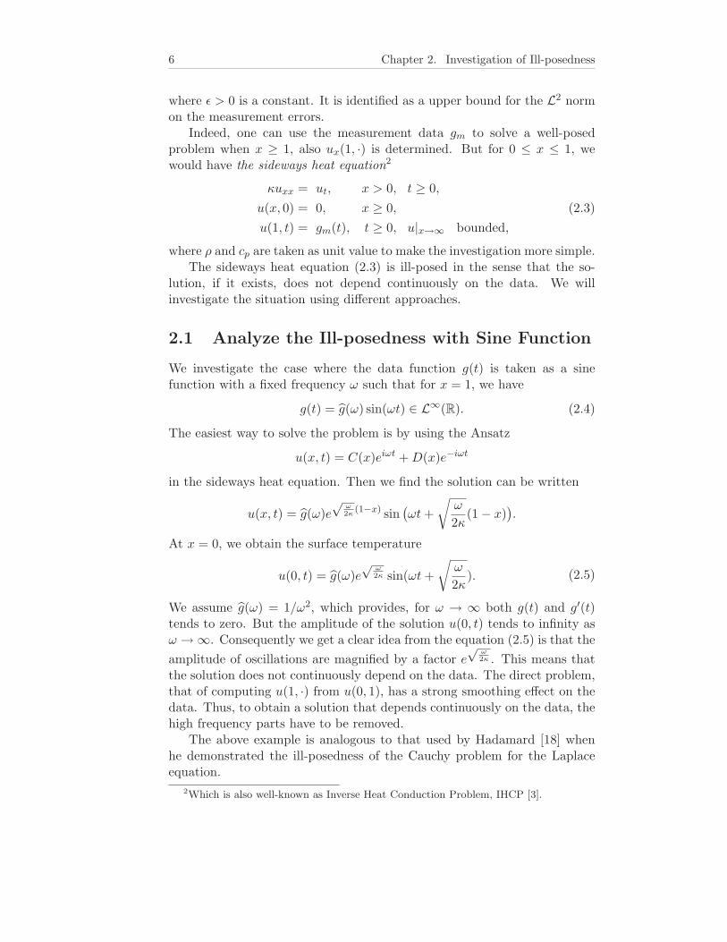
2.1 Analyze the Ill-posedness with Sine Function

We investigate the case where the data function g(t) is taken as a sinefunction with a fixed frequency ω such that for x = 1, we have

g(t) = g(ω) sin(ωt) ∈ L∞(R). (2.4)

The easiest way to solve the problem is by using the Ansatz

u(x, t) = C(x)eiωt + D(x)e−iωt

in the sideways heat equation. Then we find the solution can be written

u(x, t) = g(ω)e√

ω2κ

(1−x) sin(ωt +

√ω

2κ(1 − x)

).

At x = 0, we obtain the surface temperature

u(0, t) = g(ω)e√

ω2κ sin(ωt +

√ω

2κ). (2.5)

We assume g(ω) = 1/ω2, which provides, for ω → ∞ both g(t) and g′(t)tends to zero. But the amplitude of the solution u(0, t) tends to infinity asω → ∞. Consequently we get a clear idea from the equation (2.5) is that the

amplitude of oscillations are magnified by a factor e√

ω2κ . This means that

the solution does not continuously depend on the data. The direct problem,that of computing u(1, ·) from u(0, 1), has a strong smoothing effect on thedata. Thus, to obtain a solution that depends continuously on the data, thehigh frequency parts have to be removed.

The above example is analogous to that used by Hadamard [18] whenhe demonstrated the ill-posedness of the Cauchy problem for the Laplaceequation.

2Which is also well-known as Inverse Heat Conduction Problem, IHCP [3].

2.2. Ill-posedness Analysis in the Fourier Space 7

2.2 Ill-posedness Analysis in the Fourier Space

In order to investigate the ill-posedness in the Fourier domain, we are onlyinterested to find a solution in the finite time interval 0 ≤ t ≤ T . Since wehave no idea about t ≥ T , we assume that the surface temperature dropsdramatically to zero for all t ≥ T . Moreover, to simplify the analysis wedefine all functions to be zero for t < 0. Let g be the Fourier transform ofexact data function g,

g(ξ) =1√2π

∫ ∞

−∞g(t)e−iξtdt, −∞ < ξ < ∞. (2.6)

Now, suppose that the Fourier transform of F on R = (−∞,∞) is

F[F (η)] = F (ζ),

then differentiation takes F (ζ) to iζF (ζ). Therefore, by taking Fourier trans-form of (2.1) we get the corresponding equations in the frequency domain[14, 28, chapter 7, 4]:

κuxx(x, ξ) = iξu(x, ξ), x > 0 and ξ ∈ R,

u(1, ξ) = g(ξ), ξ ∈ R,

u(·, ξ)|x→∞ bounded.

(2.7)

This is a family of ordinary differential equations parameterized by ξ. Byusing the Ansatz u(x) = cemx and plugging into (2.7) the general solutioncan be obtained in the form

u(x, ξ) = C1(ξ)ex

q

iξ

κ + C2(ξ)e−x

q

iξ

κ , (2.8)

where√

iξ denotes the principal value of the square root,

√iξ =

(1 + i)

√|ξ|2 , ξ ≥ 0,

(1 − i)

√|ξ|2 , ξ < 0.

Since the real part of√

iξ is positive, we can see that the exponential func-

tion, the first term ex

q

iξ

κ in right side of (2.8), grows rapidly as x tends toinfinity. Therefore, to find a bounded solution at infinity, we conclude thatC1(ξ) = 0. The equation (2.8) now be simplified by using the boundarycondition x = 1,

u(1, ξ) = C2(ξ)e−

q

iξ

κ ,

yields

g(ξ) = C2(ξ)e−

q

iξ

κ ,

8 Chapter 2. Investigation of Ill-posedness

which leads to

C2(ξ) = e

q

iξ

κ g(ξ).

Hence the equation (2.8) provides the solution

u(x, ξ) = e

q

iξ

κ(1−x)

g(ξ). (2.9)

In order to obtain the solution (2.9) we have bound on the solution at infinity.Since the real part of

√iξ is positive, and the solution u(x, ξ) is assumed to

be in L2(R), we see that the exact data function, g(ξ), must decays rapidlyas ξ → ∞.

Since we measured the temperature by measurement device, there wouldhave some measurement errors. Hence, we assume that

gδm(t) = g(t) + δ(t), (2.10)

where δ ∈ L2(R) is a small measurement error. The Fourier domain if weuse gm as data function, we get the following solution

w(x, ξ) = ex

q

iξ

κ(1−x)

g(ξ) + δ(ξ),

This leads to

w(x, ξ) = u(x, ξ) + ex

q

iξ

κ(1−x)

δ(ξ). (2.11)

In the solution w(x, ξ), since the measurement error δ(ξ) do not have thesame decay in frequency as much as the actual data g(ξ), the solution w(x, ξ)will not, in general, be in L2(R). Thus the ill-posedness can easily be ob-served in the blow-up of high frequency perturbations in the data when

the equation (2.3) is solved numerically. Since the factor e√

|ξ|/2κ magnifythe frequency components of (2.9), thus it might be said that the degree ofill-posedness depends on the coefficient κ.

2.3 Standardization of the Region

In solving mathematical modelling problems using partial differential equa-tions it is almost always wise to rewrite the equations into the dimensionlessforms. By taking the proper choice of dependent and independent variablesone can modify the original problem to the dimensionless form. Here wewill scale both the time and space variables. We consider the heat equationin the linear form

ρcp∂u

∂t= κ

∂2u

∂x2, x > 0, t ≥ 0, (2.12)

where cp is the specific heat, ρ is the density and κ is the thermal conductiv-ity of the material which are all constants. For a physical situation, u(x, t)

2.3. Standardization of the Region 9

is the temperature inside the body and g(t) is the recorded temperaturemeasured at a distance x = L from the surface of the body. In practice, g(t)can only be measured for a finite time interval 0 ≤ t ≤ T . We introducedimensionless space coordinate ξ and time co-ordinate τ as follows:

ξ =x

L, and τ =

t

T.

Now, through the scaling, derivatives of original model can be transformedto derivatives of the dimensionless variables. By applying Euler’s chain rulewe then have the required form

∂u

∂τ= K

∂2u

∂ξ2, (2.13)

where K = κTρcpL2 is a constant.

For the measurement data, the function g is considered to be known onthe interval 0 ≤ t ≤ 1. It can be observed that, when the value K decreasesthe degree of ill-posedness increases. Therefore for a smaller value of L wewould have better stability properties of the problem. Indeed, the value ofK also depends on T . Thus in measuring the data on a finite time intervalone might deduce, that the length of interval can influence the stabilityproperties of the problem. In fact, this is actually not the case. we canintroduce a standard property of the Fourier transform

g(Tt)(ξ) =1

Tg(

ξ

T).

Based on this property we can make a conclusion, that any attempt toincrease the stability by using a larger T will cause the scaled data functionto be spread out in the frequency domain, consequently it would be difficultfor someone to solve the problem.

It is noticeable, although we seek to recover u only for 0 ≤ x < 1, theproblem specification includes the heat equation for x > 1, together with theboundness of the solution u(x, t) at infinity. Since we can obtain u for x > 1by solving a well-posed quarter plane problem, also ux(1, ·) is determined.Thus the problem (2.3) usually have the form on the line x = 1,

κuxx = ρcp ut, 0 < x < 1, 0 < t < 1,

u(1, t) = g(t),

ux(1, t) = h(t),

u(x, 0) = 0,

(2.14)

and, the solution of this problem can be expressed u(x, t) = w(x, t)+v(x, t),

10 Chapter 2. Investigation of Ill-posedness

where w(x, t) be the solution of well-posed problem

κwxx = ρcp wt, 0 < x < 1, 0 < t < 1,

w(0, t) = 0,

wx(1, t) = h(t),

w(x, 0) = 0,

(2.15)

and v(x, t) be the solution of ill-posed problem

κvxx = ρcp vt, 0 < x < 1, 0 < t < 1,

v(1, t) = g(t) − w(1, t),

vx(1, t) = 0,

v(x, 0) = 0.

(2.16)

Hence, from the above presentation it might be concluded that we can solvethe inverse heat conduction problem (SHE) from a quarter plane problemby considering an appropriate length of the region, where we would havethe measurement data g(t) and the heat flux h(t) by solving the well-posedproblem, in the x-direction.

Chapter 3

Stabilizing Assumptions

The idea of stabilization is an important concept for any type of ill-posedproblem. A stable approximation means small perturbations in the mea-surement data cause only small perturbations in the solutions. It meansthat the solution always depends continuously on the data. In the wholesection we will discuss how to reconstruct the problem by imposing a prioribound on the solution data, and also how to get a solution that must con-tinuously exist on the data. We already found the solution operator definedby (2.9) is unbounded, that is, the problem is ill-posed. In order to makethe solution stable we have to impose a priori bound M on the solution atx = 0, such that, ‖u(0, ·)‖ ≤ M. Thus, by considering some imprecisions inthe matching of the data we can approximate the problem (2.3) by,

κuxx = ut, x > 0, t ≥ 0,

u(x, 0) = 0, x ≥ 0,

‖u(1, ·) − gδm(·)‖ ≤ ǫ,

‖u(0, ·)‖ ≤ M.

(3.1)

We will show that any two solutions of the equation (3.1), say u1 and u2,from the given data g(t) at x = 1 with ‖ui(1, ·)− gδm(·)‖ ≤ ǫ, and prescribedbound ‖u(0, ·)‖ ≤ M at x = 0, satisfy the following inequality

‖u1(x, ·) − u2(x, ·)‖ ≤ 2M1−xǫx, (3.2)

where ǫ,M > 0 are both known and ǫ << M.The convexity inequality is considered for stabilizing the ill-posed con-

tinuation problem when the data function g contains some perturbations.The inequality defined by (3.2) was first proved by [21]. Also a useful pre-sentation on convexity inequality can be found in [8]. Our presentation isbased on that in [4]. Indeed, the degree of ill-posedness is stabilized by theuse of such bound together with the analysis of resulting continuity withrespect to the data. The estimate (3.2) is an approximation of Logarithmic

Hussain, 2010. 11

12 Chapter 3. Stabilizing Assumptions

Convexity type. In the rest of this section, we will first define the concept oflogarithmical convexity, and the proof of inequality (3.2) will be given lateron.

3.1 The Proof

Definition 3.1.1. A function φ defined on a convex subset of a real vectorspace and taking positive values is said to be logarithmically convex if log φ(x)is convex function of x.

If φ > 0 and φ is log convex on an interval [Ω1, Ω2], then the inequality

log φ(x) ≤ (1 − γ(x)) log φ(Ω1) + γ(x) log φ(Ω2), x ∈ [Ω1, Ω2],

holds for γ(x) = Ω2−xΩ2−Ω1

.The inequality can be rewritten as

φ(x) ≤ φ(Ω1)(1−γ(x))φ(Ω2)

γ(x), x ∈ [Ω1, Ω2]. (3.3)

Moreover, a non-negative C2 function φ is log convex if and only ifφφ′′−(φ′)2 ≥ 0. This is a consequence of the fact that a function φ is convexif its second order derivative is positive

(log(φ))′′ =φφ′′ − (φ′)2

φ2≥ 0, ⇐⇒ φφ′′ − (φ′)2 ≥ 0.

In this paper, we use the log convex function for error estimates. Thusit is necessary to allow such functions to have zeros.

Lemma 3.1.2. Let φ(x) be continuous, nonnegative and log convex on theinterval Ω. Then φ(x) > 0 on Ω or φ(x) ≡ 0 on Ω.

Proof. Suppose that φ(x) > 0, for some x ∈ Ω. We shall prove that φ > 0in the whole interval. If φ has zeros in Ω, then due to the continuity thereexists an s1 ∈ Ω such that

φ(s1) = 0, and φ(s2) > 0, s2 ∈ (s1, x].

Let ǫ > 0 be given and choose a ξ ∈ (s1, x) such that φ(ξ) < ǫ.Since φ is a log convex and φ > 0 on [ξ, s1] we find that for s2 ∈ [ξ, s1], wehave

φ(s2) ≤ φ(ξ)ψ(s2)φ(x)1−ψ(s2)

≤ ǫψ(s2)φ(x)1−ψ(s2),

where φ(s2) = x−s2x−ξ 6= 0.

Since ǫ can be arbitrarily small we conclude that φ(s2) = 0, s2 ∈ (s1, x)and since φ is continuous also φ(x) = 0, this contradicts the assumptionthat φ(x) > 0, hence φ has no zeros in Ω. This means that either φ = 0 orφ > 0 .

3.1. The Proof 13

Lemma 3.1.3. Let φ1 and φ2 are continuous, non-negative and log convexon an interval Ω. Then φ1 +φ2 also has the same properties on the intervalΩ.

Proof. We shall prove the sum by applying Holder’s inequality. We have toshow that the inequality (3.3) holds for every subinterval [Ω1, Ω2] ⊂ Ω. Forsimplicity we may assume that [Ω1, Ω2] := [0, 1]. Let x ∈ (0, 1), then

φ1(x) + φ2(x) ≤ φ1(0)xφ1(1)1−x + φ2(0)xφ2(1)1−x

≤

φ1(0)xp + φ2(0)xp 1

p

φ1(1)(1−x)q + φ2(1)(1−x)q 1

q,

where 1p + 1

q = 1. If we substitute p = 1x , we then get

φ1(x) + φ2(x) ≤

φ1(0) + φ2(0)x

φ1(1) + φ2(1)1−x

.

Hence φ1 + φ2 is log convex.

We can now prove the inequality (3.2), and the proof presented here isa simplified version of a more general result by Levine [21, sec.3].

Theorem 3.1.4. Let u1 and u2 be two solutions of the problem (3.1). Then

‖u1(x, ·) − u2(x, ·)‖ ≤ 2M1−xǫx, 0 ≤ x ≤ 1. (3.4)

Proof. For simplicity we use κ = 1, for equation (3.1), in the proof. Letw = u1−u2, and φ(x) = ‖w(x, ·)‖2. So we can define w(x, ξ) at x = 1, usingthe idea of equation (2.9), as

w(x, ξ) = e√iξ(1−x)w(1, ξ).

By applying Parseval relation we determine that

φ(x) =

∫ ∞

−∞|w(x, ξ)|2dξ =

∫ ∞

−∞e√

2|ξ|(1−x)|w(1, ξ)|2dξ.

Using the concepts, described in definition (3.1.1), we have

φ(x)φ′′(x) − (φ′(x))2 =( ∫ ∞

−∞|w(x, ξ)|2dξ

)( ∫ ∞

−∞(2 |ξ|)|w(x, ξ)|2dξ

)

−( ∫ ∞

−∞

√(2 |ξ|)|w(x, ξ)|2dξ

)2 ≥ 0,

where the last inequality follows from the Cauchy-Schwarz inequality. Thismeans that ‖w(x, ·)‖2 is log convex. Thus we obtain

‖u1(x, ·) − u2(x, ·)‖2 ≤(‖u1(0, ·) − u2(0, ·)‖2

)1−x(‖u1(1, ·) − u2(1, ·)‖2)x

.

14 Chapter 3. Stabilizing Assumptions

If we impose the priori bound ‖ui(0, ·)‖ ≤ M for i = 1, 2 on the solution,and apply the condition ‖ui(x, ·)−gδm(·)‖ ≤ ǫ, then by the concept of triangleinequality we finally obtain

‖u1(x, ·) − u2(x, ·)‖ ≤ 2M1−xǫx,

which completes the proof of (3.4).

The above theorem proves that we have a stable dependence on the datafor the problem (3.1) in the sense (3.2), and so we call (3.1) a stabilizedproblem. The inequality (3.4) is sharp (cf. 4.1), thus we can not expect tofind a numerical method which satisfy for a better error estimate for approx-imating solutions of (3.1). But one difficulty of (3.1) is that it does not haveuniqueness. Therefore, in order to find a useful numerical procedure it isconvenient to modify the problem by choosing some parameters dependenceon both ǫ and M.

Chapter 4

Regularizations

In this section we will study how to stabilize the sideways heat equation bycutting off high frequencies from the solution. It means that the ill-posedproblem will be regularized. A variety of numerical and analytical tech-niques have been developed, e.g. [7, 17], to find stable solutions for theinverse heat conduction problems. We usually in common have some meth-ods like Tikhonov regularization method, mollification method, Alifanov’siterative regularization method and the method of Beck. Here we considera regularization method in the Fourier space by cutting off high frequenciesfrom the solution. Similar approach of the method can be found in [4, 25].We introduce the problem in Fourier space parameterized by ξ,

κuxx(x, ξ) = iξu(x, ξ), x > 0 and ξ ∈ R,

u(1, ξ) = g(ξ), ξ ∈ R,

u(·, ξ)|x→∞ bounded.

(4.1)

It has a solution in the Fourier domain, already illustrated in section 2, ofthe form

u(x, t) =1√2π

∫ ∞

−∞e

q

iξ

κ(1−x)

g(ξ)eiξtdξ. (4.2)

Since the principal value of√

iξ in the term e

q

iξ

κ(1−x)

has a positive realpart, small error in high frequency components can blow-up and completelydestroy the solution for 0 ≤ x < 1. A natural way to stabilize the problem isto remove all high frequencies from the solution and instead consider (4.1)only for |ξ| < ξmax. Then we have the regularized solution defined by therelation

w(x, ξ) = Xmaxu(x, ξ),

which yields to the form

w(x, t) =1√2π

∫ ∞

−∞e

q

iξ

κ(1−x)

g(ξ)Xmax eiξtdξ, (4.3)

Hussain, 2010. 15

16 Chapter 4. Regularizations

where Xmax is the characteristic function of the interval [−ξmax, ξmax].In real applications, instead of having exact data g we would actually

have an access only for some approximation gm of g, where the perturbationcan be defined

δ = g − gδm,

and let wδ(x, t) be the regularized solution defined by (4.3) with the mea-sured data gδm. The difference between exact solution u(x, t) and regularizedsolution can be divided into two parts,

‖u(x, ·) − wδ(x, ·)‖ ≤ ‖u(x, ·) − w(x, ·)‖ + ‖w(x, ·) − wδ(x, ·)‖= RT + RX ,

(4.4)

where RT and RX are defined

R2T =

∫

|ξ|>ξmax

|u(x, ξ)|2dξ, and, R2X =

∫ ξmax

−ξmax

|w − wδ|2dξ,

=

∫ ξmax

−ξmax

|eq

iξ

κ δ(ξ)|2dξ.

In the regularization process these two terms behave differently. The trunca-tion error RT , is a measure of the effect of the introduced cut off frequency.By increasing ξmax we include a larger part of the spectrum in the solution,and thus we reduce the truncation error. We have also propagated dataerror RX , is generated by the inexact data. If we increase ξmax, then RXwill eventually dominate the solution. Thus the total error depends on theeliminating part of the frequency, ξmax.

In fact, we would have some optimal cut off frequency, but we can notdetermine it explicitly since it depends on unavailable information about theexact data g, e.g. the smoothness and on the errors in the data. However,it is possible to give a parameter choice rule which, given some a prioriinformation about the solution, leads to a convergent scheme [17, section 3],that is,

‖u(x, ·) − wδ(x, ·)‖ → 0, if ‖δ‖ → 0.

For solving the ill-posed problems, such a scheme is referred to as a regu-larization method in [17]. It is necessary to investigate the quality of ourmethod using the perturbed data gδm. In the following sections we will dis-cuss about ‘parameter choice rule’ by deriving an error estimate for theapproximate solution (4.3).

4.1 Error Estimate

In general, it is impossible to determine the solution of an ill-posed problemwithout knowing any information of the error level [1, 30], to get the error

4.1. Error Estimate 17

estimate for an approximate solution [1, 29] and even to get a rate of conver-gence for approximate solutions on the whole infinite dimensional Banachspace [1]. So it would be convenient to have all available a priori informationabout the exact solution for constructing a set of rules with special prop-erties. In this section we illustrate such a bound on the difference betweenunbounded operator u(x, ·) and bounded operator w(x, ·) of (4.2) and (4.3)respectively. We assume that we have an a priori bound ‖u(0, ·)‖ ≤ M onthe exact solution of the problem (4.1), where δ ≥ 0 be an error level ofu(1, ·), is supposed to be known.

Now we will investigate some error bound conditions using the regular-ized solutions, say, w1 and w2 of (4.3) by the following lemmas.

Lemma 4.1.1. Suppose that we have two regularized solutions w1 and w2

defined by (4.3) with data g1 and g2, satisfying ‖g1 − g2‖ ≤ ǫ. If we selectξmax = 2κ(log(M/ǫ))2, then we get the bound

‖w1(x, ·) − w2(x, ·)‖ ≤ M1−xǫx. (4.5)

Proof. In order to obtain L2 estimates for the difference w1(x, ·)−w2(x, ·),we may introduce Parseval relation. Then we have

‖w1(x, ·) − w2(x, ·)‖2 =

∫ ∞

−∞|w1(x, t) − w2(x, t)|2 dt

=

∫ ∞

−∞|w1(x, ξ) − w2(x, ξ)|2 dξ

= ‖w1 − w2‖2

=

∫ ξmax

−ξmax

∣∣∣∣eq

iξ

κ(1−x)

(g1 − g2)

∣∣∣∣2

dξ

≤∣∣∣∣e

q

iξmaxκ

(1−x)∣∣∣∣2

‖g1 − g2‖2

= e

q

2ξmaxκ

(1−x)‖g1 − g2‖2.

Using ξmax = 2κ(log(M/ǫ))2, we finally obtain

‖w1 − w2‖ ≤ M1−xǫx.

From Lemma 4.1.1 we observe that the regularized solution (4.3) contin-uously depends on the input data. In the next lemma we will examine thedifference between (4.2) and (4.3) using the exact data g(t).

Lemma 4.1.2. Suppose, u and w be the solutions defined by (4.2) and (4.3)with the same exact data g, and let ξmax = 2κ(log(M/ǫ))2. If ‖u(0, ·)‖ ≤ Mthen

‖u(x, ·) − w(x, ·)‖ ≤ M1−xǫx. (4.6)

18 Chapter 4. Regularizations

Proof. In order to obtain L2 estimates for the difference u(x, ·) − w(x, ·),we may introduce Parseval relation and consider the fact, that the solutionscoincide for ξ ∈ [−ξmax, ξmax]. we have

‖u(x, ·) − w(x, ·)‖2 =

∫ ∞

−∞|u(x, t) − w(x, t)|2 dt

=

∫ ∞

−∞|u(x, ξ) − w(x, ξ)|2 dξ

=

∫

|ξ|>ξmax

∣∣∣∣eq

iξ

κ(1−x)

g(ξ)

∣∣∣∣2

dξ

≤ e−x

q

2ξmaxκ

∫

|ξ|>ξmax

∣∣∣∣eq

iξ

κ g(ξ)

∣∣∣∣2

dξ

≤ e−x

q

2ξmaxκ

∫

|ξ|>ξmax

|u(0, ξ)|2 dξ

≤ e−x

q

2ξmaxκ ‖u(0, ·)‖2.

Finally, we use the a priori error bound ‖u(0, ·)‖ ≤ M together with thefrequency ξmax = 2κ(log(M/ǫ))2 , the unknown solution leads to the errorbound

‖u − w‖ ≤ M1−xǫx.

Now we have all information to formulate the major part of this section.Throughout the following theorem, we will observe that the regularized so-lution wδ(x, t) is actually an approximation to the actual solution u(x, t).From the relation (3.2) we can also conclude that the approximation er-ror depends continuously on the measurement error. Similar survey can beviewed in [4].

Theorem 4.1.3. Let u be the solution (4.2) with exact data g and wδ thesolution (4.3) with measured data gδm. If we have a bound ‖u(0, ·)‖ ≤ Mand the measured function gδm satisfies ‖g − gδm‖ ≤ ǫ and also if we chooseξmax = 2κ(log(M/ǫ))2, then we get the error bound

‖u − wδ‖ ≤ 2M1−xǫx. (4.7)

Proof. Let wδ be the solution described by (4.3) with exact data g. Usingthe inequality

|p + q|2 ≤ |p|2 + |q|2 + 2|p||q| ≤ 2(|p|2 + |q|2),together with the previous two Lemmas, we obtain

‖u − wδ‖ ≤ ‖u − w‖ + ‖w − wδ‖ ≤ 2M1−xǫx.

4.1. Error Estimate 19

It is noticeable, that, the sharpness of the inequality (4.6) depends onlyon the spectral contents of the exact solution. Now

‖u(x, ·)‖2 ≈ e−x

q

2ξmaxκ

∫

|ξ|≥ξmax

|u(0, ξ)|2 dξ,

if the support of u(0, ξ) is localized close to the cut-off frequency, conse-quently the estimate, in Lemma 4.1.2, can be very tight. On the otherhand,

∫ ξmax

−ξmax

∣∣∣∣eq

iξ

κ(1−x)

(g − gδm)

∣∣∣∣2

dξ ≈ e

q

2ξmaxκ

(1−x)‖g − gδm‖,

if the support of the measurement error (g − gδm) is localized close to ξmax.Hence, we make a statement that, the Lemma 4.1.2 necessarily gives a

sharp inequality, and for any case, we can not expect a better error estimatethan that in 4.1.3. We can also find a handy discussion on sharpness of theestimate (4.7) in [21, 7].

Next, we will discuss some error bounds on the heat flux ux for thedomain 0 < x < 1. From (4.2), we also obtain a formula for the gradientux(x, t) by differentiating with respect to x inside the integral. We mayhave,

ux(x, t) = − 1√2π

∫ ∞

−∞

√iξ

κe

q

iξ

κ(1−x)

g(ξ)eiξtdξ. (4.8)

From (4.2) and (4.8) we find a relation between h and g,

h(ξ) = −√

iξ

κg(ξ)

We obtain error bounds in the L2-norm for temperature gradient h :=ux(1, ·) to the approximated measured data hm at x = 1.

Corollary 4.1.4. Let 0 < x < 1. Let u and wδ are defined as in Theorem4.1.3. Suppose that we have a bound ‖ux(0, t)‖ ≤ Md, and that the measuredtemperature gradient hm satisfies ‖h − hδm‖ < ǫd, and that we chooseξmax = 2κ(log(Md/ǫd))

2, then we get the error bound

‖ux − wδx‖ ≤ 2M1−x

d ǫxd. (4.9)

In the sense of Holder continuity on L2 space, we conclude that a com-puted temperature gradient depends continuously on the data.

20 Chapter 4. Regularizations

Chapter 5

Numerical Implementation

for the SHE

The problem of solving the sideways heat equation (SHE) the solution isseverely ill-posed in the sense that the solution does not depend continuouslyon the data. The situation is actually caused by the time derivative which isan unbounded operator. Therefore we can obtain well-posed behavior of anill-posed problem by substituting ∂

∂t with a bounded approximation. Thusit is convenient to establish a numerical implementation of the problem bydiscretizing space and time separately.

In this section we consider the time variable with equidistant grid points,and search for an approximation of ∂

∂t by using discretized Fourier Trans-form of the problem. Numerical methods, based on approximating the timederivative, have been considered by Elden [12, 11], by Elden and Reginskaand Berntsson [13], see also [4].

5.1 A Method of Lines

The space discretization scheme should be selected independently of thetime discretization. Therefore it is assumed that a time grid and a matrixrepresenting the ∂

∂t have been selected. We illustrate in this section, thatthe resulting problem can be solved numerically, essentially as an ordinarydifferential equation in the space variable. In our implementation, the timederivative is computed by a spectral approximation or a spline function, andwill be discussed more details later in this section. Now, we consider the“initial-value” problem in the linear form

(u

κux

)

x

=

(0 κ−1I∂∂t 0

)(u

κux

), 0 < x < 1, 0 ≤ t ≤ 1, (5.1a)

with initial-boundary values

u(1, t) = gδm(t), ux(1, t) = hδm(t), 0 ≤ t ≤ 1, (5.1b)

Hussain, 2010. 21

22 Chapter 5. Numerical Implementation for the SHE

u(x, 0) = 0. 0 < x < 1. (5.1c)

The initial values for ux can be computed numerically by solving the well-posed quarter plane problem with data u(1, t) = gδm(t) for x ≥ 1. In a formalmanner the solution of the system (5.1) can be written

(u

κux

)= e−B(1−x)

(gδm(t)

κhδm(t)

),

where B is an unbounded operator defined as

B =

(0 κ−1I∂∂t 0

).

We already analyzed that the sideways heat equation (2.3) is severely ill-posed. The same phenomenon can be observed in the frequency domain byreplacing (5.1a) with a family of ordinary differential equations parameter-ized by ξ. It is easily verified that the matrix corresponding to B is

Bξ =

(0 κ−1

iξ 0

).

The eigenvalues of Bξ are ±√

iξκ . Therefore the spectrum of the operator B

is unbounded in the left-half plane. It implies that the operator e−B(1−x) isalso unbounded and consequently solving (5.1) is an ill-posed problem, highfrequency noise can blow up and completely destroy the numerical solution.Even if the data are filtered [7, 23], so that, the high frequency perturbationsare removed, the problem is still ill-posed: rounding errors introduced in thenumerical solution will be magnified and make the accuracy of the numericalsolution deteriorate as the initial value problem is integrated. The methodshave been investigated in different papers [12, 11, 13, 4] for solving thesideways heat equation numerically, where to obtain a well-posed problemthe unbounded operator ∂

∂t have to be bounded. Thus we essentially replace∂∂t with a bounded approximation.

Although the differential equation is valid for all t ∈ R but, in realapplications, data are only available for a finite period of time. In ourcase we normalized the data t ∈ [0, 1]. Thus by discretizing (5.1a) on anequidistant grid tkn−1

k=0 ∈ [0, 1], we obtain an initial-value problem for anordinary differential equation,

(U

κUx

)

x

=

(0 κ−1ID 0

) (U

κUx

), 0 ≤ x ≤ 1, (5.2)

with initial data,

U(1) = Gδm, Ux(1) = Hδ

m

5.2. Time Derivative Discretization 23

where the matrix D is discretization of the time derivative; U = U(x) andUx = Ux(x) are semi-discrete representations of the solution and its deriva-tive. That is,

U(x) ≈(u(x, t1), u(x, t2), . . . , u(x, tn)

)T,

and,

Ux(x) ≈(ux(x, t1), ux(x, t2), . . . , ux(x, tn)

)T,

and, Gδm and Hδ

m are vectors containing samples from gδm and hδm respec-tively on the grid. Thus (5.2) can be considered as a method of lines [16, 20].The discretized system (5.2) can be solved using some standard method. Weuse an explicit fourth order Runge-Kutta method for solving the system ofequations (5.2) which works well. It can also found in [12] that it is sufficientto use an explicit method, e.g. ode45 in Matlab, based on RK method.

It is noticeable that, the approach, a method of lines, is easy to generalizeto more general equations. We can solve the initial value problem for any κ,where κ can only be a constant, it can only depend on x, it can also dependon both x and U . For a non linear system of ordinary differential equations,i.e., κ := κ(x, U), and taking V = κ(x, U)Ux, we have

(U

V

)

x

=

(0 κ(x, U)−1ID 0

)(U

V

), 0 ≤ x ≤ 1, (5.3)

with initial data,

U(1) = Gδm, and V (1) = κ(1, Gδ

m)Hδm,

where κ(x, U) = diag(κ(x, U1), . . . , κ(x, Un)

)is a diagonal matrix. For sim-

plicity, we assume in this discussion for the nonlinear problem (1.1) thatρ(U) = cp(U) = 1.

Note also that, if D represents a discrete approximation of the timederivative, then D is a bounded operator [12, 11, 13]. Thus the problem ofsolving (5.3) is, in principle, a well-posed initial value problem. However, theoriginal problem is ill-posed, and for a fine discretization (5.3) can extremelybe ill-conditioned [19].

In the following sections we will discuss the approximation of the timederivative D by using some methods.

5.2 Time Derivative Discretization

Methods for approximating the time derivative, the matrix D in (5.3), havebeen considered in different papers. For example, discretization using finitedifferences was considered in [11, 12], Galerkin approximation using waveletsin [4, 13], a spectral approximation in [25, 13] and a method based on theapproximation by cubic splines in [4]. In this section we have a discussion onthe approximated derivative based on a spectral method and cubic splines.

24 Chapter 5. Numerical Implementation for the SHE

5.2.1 A Spectral Method in the Finite Fourier Space

A spectral approximation is the approach, to write the numerical solutionas a finite expansion in terms of some known type of functions, where thebasis functions are associated with the spectrum of some operator [15]. Now,to deal with periodic solutions, a natural choice of basis functions can betrigonometric polynomials. This leads to Fourier methods, such as, DiscreteFourier Transform (DFT) that provides the decomposition of a vector inRn in terms of the frequency components. Thus we can use the DFT toeliminate all high frequencies, i.e., |ξ| > ξmax, where ξmax is the cut-off level.A use of this method was proposed in different papers, e.g. [4, 13, 25]. Weexplain the DFT for approximating the derivative in details in the followingparagraphs.

The DFT can be used to obtain very accurate approximations of thederivative of smooth functions. It is a linear mapping that operates on com-plex n-dimensional vectors in much the same way that the Fourier transformoperates on functions on R [14, chapter 7]. To motivate it, we consider theproblem of numerical approximation of Fourier transforms.

In order to use the Fourier transform

g(ξ) =1√2π

∫ ∞

−∞g(t)e−iξtdt,

in numerical computations, we must approximate it by something that in-volves only a finite number of algebraic calculations performed on a finiteset of data. This work is done in several steps.

First, we replace the integral over [−∞,∞] by the integral over a finiteinterval. In other words, we assume that g vanishes outside some boundedinterval [r, r + δ]. It will be convenient to assume that r = 0, which canalways be achieved by replacing g(t) by g(t − r) [14, chapter 7].

Next, we try to calculate g(ξ), not at every ξ ∈ R but only at a finitesequence of points contained in some bounded interval [−C, C]. We intro-duce the trigonometric interpolation of 2π-periodic functions u(x, ·) thatare known in the finite interval ∈ [0, 1] at grid points tk = kht, such that,uk = u(x, tk) for k = 0, 1, . . . , n − 1, where ht is the step size in the timescale. Assuming that n is an even number with nht = 2π, we write theapproximation

u(x, t) =1√2π

n/2−1∑

k=−n/2uke

iξkt, (5.4)

where ξk = 2πk. Thus under the interpolation condition

u(x, tk) = uk, k = 0, 1, . . . , n − 1,

5.2. Time Derivative Discretization 25

the coefficients are given by [15, chapter 12],

uk =1√2π

n−1∑

k=0

uke−iξktkht, k = −n/2,−n/2 + 1, . . . , n/2 − 1. (5.5)

This is the Discrete Fourier Transform. If we differentiate the interpolatingfunction (5.4), and denote ut(x, t) = v(x, t), we then have

v(x, t) =1√2π

n/2−1∑

k=−n/2vke

iξkt =1√2π

n/2−1∑

k=−n/2iξkuke

iξkt,

The trigonometric interpolation is very accurate for smooth functions, bothfor the function itself and for its derivatives [15, chapter 12]. If u(x, ·) isknown only at the grid points, we want to compute approximations of ∂u

∂tat the grid points as well. Hence the algorithm is1. Compute uk, k = −n/2,−n/2 + 1, . . . , n/2 − 1 by the DFT2. Compute vk = ikuk, k = −n/2,−n/2 + 1, . . . , n/2 − 13. Compute vk, k = 0, 1, . . . , n−1 by the inverse discrete Fourier transform

In general, when the discrete Fourier transform is carried out by using thefast Fourier transform, the operation count of the numerical differentiationis O(n logn). However, we compute the derivative by executing the abovesteps. Hence the regularized solution (4.3) can be computed by solving (5.2),with the matrix D ≡ DF defined by

DF = FHΛFF,

where F is the Fourier matrix [22], and ΛF is a diagonal matrix definedas, ΛF = diag(iξk), corresponding to differentiation of the trigonometricinterpolant, where the frequency components with |ξ| > ξmax are explicitlyset to zero. Thus the diagonal elements of ΛF are

(ΛF )k,k =

iξmax, when |ξk| < ξmax,

0, when |ξk| ≥ ξmax,

where the ξk are defined as in (5.4). This will filter the data and removethe high frequency parts of the measurement error from the solution. Theproduct of F and a vector can be computed in O(n logn) operations usingthe Fast Fourier Transform(FFT). Thus multiplication by DF can be carriedout as a FFT, followed by a multiplication by a diagonal matrix, and finallyan inverse FFT. This work requires in total O(n logn) operations.

5.2.2 Approximating the Derivative by a Spline Function

In this section we discuss another method to approximate time derivativesof discrete functions using “cubic spline approximations”. In some cases, it

26 Chapter 5. Numerical Implementation for the SHE

β1 β2β4β3

B1

B0

B2

B-1

B3

B4

B5

β5 β7β6β0β−1β

−2β−3

Figure 5.1: The basis functions B3j (t), for j = −1, . . . , 5. Every cubic spline,

defined on the interval [β0, β4] can be written, uniquely, as a linear combi-nation of the basis functions B3

j .

is difficult to approximate the operator ∂∂t using Fourier series, e.g. when

the truncation is not periodic, instead cubic spline function can be a bet-ter choice. It often provides better approximate result compared to usingFourier series.

The accurate estimations of the derivative ∂∂t require that, the cubic

splines for approximating u(x, t) must be all piecewise cubic functions. Thecubic splines work as smooth curves with continuous first and second deriva-tives, and are associated to go through a set of points. In this process thewhole interval is divided into a set of subintervals. Moreover, each splinecurve of every subinterval is a third-degree polynomial, which are normallydifferent cubic polynomial curve. These pieces of curves are so well matchedwhere they are glued for every subinterval. We now illustrate the numer-ical procedure for the approximations of ∂

∂t using cubic spline. A similarapproach of the method can be found in [4].

To make the procedure more easier, we substitute the function u(x, t)to u(t) for each forward step in the sideways heat equation, where u(t) isknown only for the discretized grid points tk = kht ∈ [0, 1] as uk = u(tk),k = 0, 1, . . . , n − 1, and ht is the time step size. Now, in order to obtainan accurate estimation of the derivative ∂u

∂t we first find a cubic spline s(t)

that approximates u(t), and then setting ∂u∂t ≈ ∂s

∂t . To explain the work we

5.2. Time Derivative Discretization 27

assume that, the points β−3, · · · , βN+2 be a set of coarse grid, and s(t) isa cubic spline function defined on the interval [β−3, βN+2], such that it has

natural breaks at βj and also s, ∂s∂t , and ∂2s

∂t2are continuous and smooth

for all breaks, i.e., in each subinterval [βj , βj+1] for j = −3, . . . , N + 1, thefunction s(t) is a cubic polynomial. The set of all cubic splines can berepresented using basis functions, B-spline, on the interval [β0, βN−1] suchthat

s(t) =N∑

j=−1

cjB3j (t − βj), (5.6)

where B3j (t) are the B-spline basis functions, which is nonzero on the interval

[βj−2, βj+2], and can be seen in figure 5.1.To fitting the coarse grid βj with respect to the discretize grid tk, it

is convenient to select them in such a way, so that, t0 = β0 and tn−1 = βN−1.Thus u(t) can be approximated by cubic spline s(t) in applying least-squaressense, which lead to solve the problem

minc∈RN+2

‖Ac − b‖2, (5.7)

where the elements of the matrix A and the vector b can be defined as

(A)i,j = B3j (ti), and (b)i = u(ti).

Since the basis functions B3j have compact support with the banded matrix

A has only four non-zero elements on each row, thus only O(n) operationsare needed for computing the vector c.

In the previous section 5.1 for solving the initial value problem (5.3), weneed to compute derivatives of the vector U(t), that contain the approximatetemperatures u(x, tk). The technique presented in the previous paragraphis used for this purpose.

It is remarkable, that, when we compute the approximation of the deriva-tive ∂

∂t by using a discrete operator D and by executing differentiation of ap-proximating cubic splines, a number of B-splines basis functions are used tocontrol the accuracy of the computed derivatives and also the norm of opera-tor D. In fact, for solving the discrete initial value problem (5.3), if we com-pute the derivatives very accurately by using too many basis functions withrespect to errors in the initial data, the solution can extremely be unstable.Thus, to stabilize the computations the grid parameter ∆β = min(βj+1−βj)in the coarse grid βj acts as a regularization parameter [17, 19]. The reg-ularizing effects are described by the figures, see section 7.2.

28 Chapter 5. Numerical Implementation for the SHE

Chapter 6

Numerical Analysis and

Solution Procedures for

Well-posed Nonlinear

Problems

In this section we first present a discussion on the properties of stiff problems,and then we will describe solving procedures of a well-posed nonlinear initialvalue problem numerically by using implicit methods.

The problem u′

= au+f(t) is called stiff if Re(ah∗) is large and negative,where h∗ is some measure of the time scale of the problem [26, chapter 1].

Systems of first-order equations, e.g. time dependent partial differentialequation, heat equation or diffusion equation, of the form u

′

= f(t,u) nor-mally show this stiffness behavior when the jacobian matrix fu has someeigenvalues whose real parts are large and negative. To motivate it, if A isdiagonalizable, A = P−1DP , the linear system u

′

= Au + f(t) reduces toa set of uncoupled equations of z

′

= λizi + hi(t), where the zi and hi arethe components of z = Pu and h = P f , respectively, and the λi are theeigenvalues of A. Similar discussion on stiff problems can be found in [26,chap 1].

Although Euler’s method and other explicit multi step methods can beused to solve a ordinary differential equation which is stiff, but it will requireexcessively small time steps for to stabilize the problem numerically. Insteadwe will search some other multi step methods which are well designed for stiffproblems. These are known as implicit methods. By using such methodsa stiff problem, linear or nonlinear algebraic equation, can be solved withsufficiently large time steps. For the one dimensional problem it can easily behandled, since the involved matrices are tridiagonal. It is suggested that forsolving a stiff problem numerically some 2nd order implicit methods, suchas, Adams-Moulton method also well known as Crank-Nicolson’s method,

Hussain, 2010. 29

30

Chapter 6. Numerical Analysis and Solution Procedures for Well-posed

Nonlinear Problems

and Matlab solver ode23s which is based on a modified Rosenbrock formula,can be very useful.

Next, to solve the well-posed problem we consider a nonlinear PDE in1D (heat or diffusion equation) in the general form:

∂u

∂t=

∂

∂x

(κ(u)

∂u

∂x

), 0 ≤ x ≤ 1, t ≥ 0, (6.1a)

with the Dirichlet boundary conditions:

u(0, t) = α(t), and u(1, t) = β(t), (6.1b)

and an initial condition:

u(x, 0) = 0 (6.2)

It is noticeable, in real applications, we most of the time deal with theproblems which are situated in some other interval for x-domain (for exam-ple, 0 ≤ x ≤ L or, L1 ≤ x ≤ L2). For all of such cases, we first scale theproblem into the dimensionless form, as already discussed in section 2.3, andlater on we will present the implementation of scaling in solving the problemnumerically, see chapter 7.

Indeed, the initial-boundary value problem become nonlinear due to thenonlinearity of the governing differential equations, or of the boundary con-ditions, or both. Most physical problems in science and engineering areactually nonlinear. In the case of linear problems one can always solve awell-posed problem (i.e., when κ does not depend on u) and reduce theproblem to one with the initial condition (6.2) above but that does not workfor nonlinear problems. More natural may be to assume that the problemis at steady state. Which means that

ut(x, 0) = 0. (6.3)

In the steady state case, there is no time variation in the solution. Thereforethe steady state solution satisfies the boundary value problem (BVP):

d

dx

(κ(u)

du

dx

)= 0, (6.4a)

with the boundary conditions:

u(0) = α0, and u(1) = β0, (6.4b)

In order to find a initial steady state temperature u0(x, t) for the well-posedproblem (6.1), we first solve the BVP (6.4) by using finite difference methodand next, we will solve (6.1) by discretizing space and time separately.

6.1. Space Domain Discretization 31

6.1 Space Domain Discretization

In this section we will discretize the space domain to deal with the right handside of (6.1a), the boundary conditions, and also the steady state initialcondition. In order to execute these, we use the finite difference methodby which the continuous variable x is discretized and the derivatives arereplaced by considering the difference approximations. Similar approachfor a nonlinear problem is suggested in [9]. In the following discussion wetransform the ODE problem (6.4) into an algebraic system of equations,which is in fact, can also be used for the left side of (6.1a).

We first discretize the x-interval and introduce a numbering of gridpoints:

x_0 x_1 x_i−1 x_i x_Nx_N+1xi

xN+1

0 1hx

h1/2

h1/2

xxN

x1

xi−1

xi+1

x0

where hx is constant step size over the whole discretization, and hx/2 = h1/2

in the figure. Therefore the number of inner points can be defined by therelation

hx(N + 1) = 1,

in the interval [0, 1]. By introducing a second-order formula and by usingthe central difference approximation for the first derivative, we have

du

dx(xi) =

u(xi + hx) − u(xi − hx)

2hx+ O(h2

x). (6.5)

Applying this approximation in (6.4a) we can derive

d

dx

(κ(u)

du

dx

)(xi) =

1

hx

((κ(u)

du

dx

)xi+hx/2

−(κ(u)

du

dx

)xi−hx/2

)+ O(h2

x)

=1

hx

(κ(uxi+hx/2)

uxi+hx− uxi

hx−

− κ(uxi−hx/2)uxi

− uxi−hx

hx

)+ O(h2

x).

At an arbitrary grid point xi, we define uxi= ui, which leads to

d

dx

(κ(ui)

duidx

)=

1

hx

(κ(ui+1/2)

ui+1 − uihx

−

− κ(ui−1/2)ui − ui−1

hx

)+ O(h2

x).

32

Chapter 6. Numerical Analysis and Solution Procedures for Well-posed

Nonlinear Problems

The function κ contains the values ui+1/2 and ui−1/2 for u which are actuallynot given in the grid points. Therefore from algebraic point of view

λa+1/2 =1

2(λa+1 + λa),

we then have a simple symmetric approximation with second order accu-racy throughout the grid points by setting them to the mean values of theneighboring points, that is, by linear interpolation,

ui+1/2 =1

2(ui+1 + ui), ui−1/2 =

1

2(ui + ui−1).

Thus we obtain

d

dx

(κ(ui)

duidx

)=

1

hx

(κ(ui+1 + ui

2

)ui+1 − uihx

−

− κ(ui + ui−1

2

)ui − ui−1

hx

)+ O(h2

x).

This relation is valid at all inner points, i.e., i = 1, 2, . . . , N . In order toget a matrix form, denoting by u the vector with components u1, u2, . . . , uNthen the above relation obtain to the form

d

dx

(κ(u)

du

dx

)=

1

h2x

tridiag(

κ(ui−1 + ui

2

), −

κ(ui−1 + ui

2

)+

+ κ(ui+1 + ui

2

),

κ(ui+1 + ui

2

))u. (6.6)

Now, for simplicity, we describe (6.6) to the standard form

d

dx

(κ(u)

du

dx

)= A

(κ(u∗)

)u + b, (6.7)

where the vector u∗ is different from the vector u for every forward stepthat can be formulated as

u∗ =(α(·) + u(1)

2,u(1) + u(2)

2, . . . ,

u(N − 1) + u(N)

2,u(N) + β(·)

2

)T,

and it contains (N + 1) elements, i.e., u∗ = (u∗1, u

∗2, . . . , u

∗N , u∗

N+1)T . Nor-

mally, it is reduced to be length N when it perform in the matrix operationsfor A, where A a is symmetric, positive definite, and N x N tridiagonalmatrix defined as

A =1

h2x

tridiag(

κ(u∗i+1)

, −

κ(u∗

i ) + κ(u∗i+1)

,

κ(u∗

i ))

,

and b is N -elements vector including the boundary values at x0 and xN+1

such that

b =1

h2x

(κ(u∗

1)α(·), 0, . . . , 0, κ(u∗N+1)β(·)

)T.

6.2. Time Domain Integration 33

To clarify with the notations, the vector elements κ(u∗1) and κ(u∗

N+1) areactually taken in every forward step by computing the thermal conductivityfunction κ(u) using u∗. For computing the initial steady state temperatureu(x, 0) from (6.4), we take from the vectors α(·) and β(·) the first twoelements as α0 and β0 respectively. Since the problem is nonlinear we canuse Newton-raphson iterative method to solve (6.4), where in each iterationthe jacobian, i.e., the matrix A is tridiagonal. There are some built-in solverin Matlab language, e.g. “ fsolve ”, using this solver we can solve the problem(6.4).

Further, we apply all the ideas of space discretization to compute thetemperature u(x, t) ≡ u(x, 0), a steady state temperature, in the time do-main [0, 1].

6.2 Time Domain Integration

When dealing with initial-boundary value problems, it is useful to introducethe Method of Lines (MoL), is also called semi discretization, where only thespace derivatives are discretized (the time derivatives are kept). In brief, itmeans that u(xi, t) ≈ ui(t) where ui(t) is a time-dependent solution functionis associated to the space grid point xi. Mathematically, we can define theillustration in the matrix form

du

dt= A(u)u + b(t), u(0) = u0, (6.8)

where A is a tridiagonal matrix and b(t) is a vector containing the bound-ary values. The initial vector u(0) is to be determined using (6.4). Aneffective approach to handle the solving procedure of the ODE (6.8) is that,first, discretize the space domain to yield a nonlinear system of algebraicequations, and then these equations to be solved at each time step by usingsome higher order (more than first order) implicit methods often used forthe stiff problems. In solving the well-posed problem we will apply two dif-ferent methods, which both have second order accuracy in the x and the tdirections. For the first one, we implement a recursive formula based on thetrapezoidal method, e.g. Crank-Nicolson implicit method for the nonlinearsystem of equations, and for the next one, we use “ode23s” Matlab solverbased on a modified Rosenbrock formula. The discretization of space deriva-tives are already illustrated in the previous section. Now, by applying thesetwo methods in (6.8), we compute the solution u(x, t) in the time interval[0, 1].

6.2.1 Crank-Nicolson Method for Nonlinear Problems

The discretization of space domain for (6.8) has already implemented byapplying finite difference approximation of second order, consequently we

34

Chapter 6. Numerical Analysis and Solution Procedures for Well-posed

Nonlinear Problems

have a nonlinear system of algebraic equations. Now, to linearize the equa-tions we introduce an approach, where we first compute the coefficients ofthe system at the previous k level using Newton-Raphson iterative method.Meanwhile, we would have a recursive formula by which we can computethe coefficients at the level k + 1 by lagging it one step behind, i.e., by eval-uating the coefficients at the previous level k. A presentation in details onNewton-Raphson iterative process and lagging properties by one time stepcan be found in [32, chapter 3, 9]. Now to construct the recursive formulaby the aid of Newton-Raphson iteration scheme, we consider the system ofalgebraic equations in the vector form

F(x) = 0, (6.9a)

where we need to find x = (x1, . . . , xN )T such that the system of equations,(F1(x), . . . ,FN (x)

)T= 0, is satisfied. The Taylor series expansion of the

system of equations (6.9a) is considered as

F(xj+1) = F(xj) + (∂F

∂x)(xj+1 − xj) + . . . (6.9b)

Now for solving F(xj+1) = 0 for xj+1, the truncated Taylor series gives

xj+1 = xj − (∂F

∂x)−1F(xj), (6.9c)

where

J ≡ ∂F(xj)

∂x=

∂F1

∂x1. . . ∂F1

∂xN

......

...∂FN

∂x1. . . ∂FN

∂xN

.

Equation (6.9c) defines the Newton-Raphson method of iterations. Herethe superscript j denotes the values obtained on the j’th iteration and j + 1indicates the values on the j + 1’th iteration.

In order to make the procedure more simpler to develop the desiredrecursion formula, we consider the problem (6.8) to the system of form

ut = A(u)u. (6.10)

We now introduce a Trapezoid method for the ordinary differential equation

ut = F(u), (6.11)

where the Trapezoid method can be derived from the trapezoid rule for theintegration. It has a simple form

tk+1 = tk + ht t,

uk+1 = uk +ht2

(F(tk,uk) + F(tk+1,uk+1)

),

6.2. Time Domain Integration 35

where ht is the step length for time variable. Equivalently,

uk+1 − ht2

(F(tk+1,uk+1)

)= uk +

ht2

(F(tk,uk)

). (6.12)

From (6.12) we can see that it is an implicit formula. Plugging (6.10) into(6.12), the system of equations obtain the form

uk+1 − ht2

(A(uk+1)uk+1

)= uk +

ht2

(A(uk)uk

),

equivalently

uk+1 − ht2

(A(uk+1)uk+1

)= G, (6.13)

where G = uk + ht

2

(A(uk)uk

)is known.

Thus, to find uk+1 we must solve the system of equations

F(u) = u − ht2

A(u)u − G = 0, (6.14)

where, for simplicity, we have omitted superscripts. Newton’s method nowcan be written

uj+1 = uj −(F

′

(uj))−1

F (uj), (6.15)

where (F

′)p,q

=(∂Fp∂uq

); p = 1, . . . , N, q = 1, . . . , N.

Now, since

u′

=

u1

u2...

uN

′

=

1 0 . . . 00 1 . . . 0...

......

...0 0 . . . 1

= I,

and G is independent of u, we have

F′

(u) = I − ht2

(A(u)u

)′

= I − ht2

((A(u))

′

u + A(u)I).

If we assume that A(u) is a slowly varying function of u, we can replace(A(u)

)′

by 0, and then we have

F′

(u) ≈ I − ht2

A(u).

Omitting(A(u)

)′

amounts to using Newton’s method with an approximatejacobian. It also means that we ignore the nonlinearity in this integrationstep. So with this approximation, there is no need to perform more thanone Newton iteration.

36

Chapter 6. Numerical Analysis and Solution Procedures for Well-posed

Nonlinear Problems

Let u0 be the starting value in the numerical solution of (6.14). Then

u1 = u0 −(I − ht

2A(u0)

)−1((I − ht

2A(u0))u0 − G0

)

= u0 − Iu0 +(I − ht

2A(u0)

)−1G0,

which is the same as

u1 =(I − ht

2A(u0)

)−1(I +

ht2

A(u0))u0.

Thus, the integration of the differential equation can be written

uk+1 =(I − ht

2A(uk)

)−1(I +

ht2

A(uk))uk, (6.16)

which is nothing but Crank-Nicolson finite difference method used for solvingnonlinear heat equations. It is a second order method in both the x- andthe t- direction, implicit in time, and is numerically stable specially for stiffproblems. Even if the nonlinearity is ignored in each particular integrationstep, it is taken care of over the whole integration by “lagging it behind onestep”.We now introduce the boundary conditions to give the above recurrenceequation in the more general form

uk+1 =(I − ht

2A(uk)

)−1((I +

ht2

A(uk))uk + bk), (6.17)

where the first and last elements of b contains the terms, the boundary valuesat x = 0 and x = 1 multiplied with κ(u)’s first and last elements respectively,and the rest of the elements of b are zeros. During the computation, A andb are usually changed in every next step. We have a more details about A,b and κ in the previous section. Finally, by applying the recursion formula(6.17) we can solve the nonlinear system of equations (6.8).

It is noticeable, since the boundary values are time dependent, there-fore in each time step it is needed to take care of those values. The workis normally done by introducing one dimensional interpolation, e.g. usingthe Matlab built-in function “interp1”, where a function uses polynomialtechniques and fitting the supplied data with polynomial functions betweendata points and then evaluating the appropriate function at the desiredinterpolation points.

For solving nonlinear system, such as (6.8), the computation time islonger than that resulting from any linear system, because the temperaturedependent thermal conductivity κ(u), density ρ(u) and specific heat cp(u)need to be evaluated at each time level k+1 from the previous time level k.Moreover, if the matrix A is full instead sparse, it would have comparatively

6.2. Time Domain Integration 37

a long computation time. It can be found in [9, chapter 4] for the linearsystem Au = b that, if the matrix A is sparse the machine computationstored only 3N − 2 elements instead N2 elements for full a matrix A. AlsoGaussian elimination needs about N3/3 floating point operations (flops) fora full matrix, where only about 5N flops is needed for a tridiagonal matrix.

Crank-Nicolson’s method is stable for all time-steps ht and space-stepshx. When ht is sufficiently small enough we obtain a smooth solution, butit has a drawback is that the computation normally takes much longer time.On the other hand, if ht is much larger compared to hx, it has an effectivecontribution in producing damped oscillations in the numerical solution, andcan be seen by graphical results [9, chapter 6].

6.2.2 Method of Lines Based on Solver ODE23s

In the previous sections we couple of times discussed on the method of lines,is a technique in solving partial differential equations (PDEs) replaced inODEs, where only the space derivatives are discretized and left the timevariable continuous. Through this process, a system of ordinary differentialequations has been solved by applying a numerical method for the initialvalue ordinary equations. In general, the MoL technique requires that a PDEproblem necessarily to be well-posed as an initial-value problem, e.g. Cauchyproblem, in at least one dimension, because Ordinary differential equation(ODE) and differential algebraic equation (DAE) integrators are initial-valueproblem solvers. However, we will apply “solver ode23s”, is based on amodified Rosenbrock formula is of second order, as an integrator whichis very efficient and sufficiently much faster than the ordinary backwarddifferentiation formulas for solving stiff problems [27].

In solving the ODE (6.8), the Crank-Nicolson implicit method is in factto be considered as an ordinary backward differences, where the time-step htis remained constant in the whole time integration. Whereas, in each timestep, ht is adaptively changed by the integrator ode23s, which definitelymake the procedure to the compact form. The ode23s solver is usuallybased on the typical initial-value problems

u′

= F (t, u), (6.18)

with the given initial value u(t0) = u0 on the time interval [t0, tend]. Inpractice, it usually has the more natural form can be defined by the ODEproblem (6.8). Of course, we now ready to compute the solutions u(x, t) ofthe system of equations (6.8) in the whole time integration using the interval[t0, tend] ≡ [0, 1], which is accomplished with the syntax in Matlab

[Ti, U] = ode23s(@, tspan, U0, options);

where the input and output arguments play the following role to the solver

38

Chapter 6. Numerical Analysis and Solution Procedures for Well-posed

Nonlinear Problems

input:

- odefun is such function that handle the task to evaluate the rightside of the differential equation (6.8).

- tspan is a vector that specifying time domain integration for theinterval [t0, tend].

- U0 is a initial temperature vary in each time step.

- options is associated with a family of optional parameters thatchange the default integration properties. Indeed, in some cases,ode23s solver performance can be improved and achieved a betterapproximated solutions by introducing “options” argument witha proper choice of parameters.

output:

- Ti the column vector contains each executed time step for theassembling integration, i.e., (T1, T2, · · · , Tend)

T ∈ [t0, tend].

- U be the approximated solution array, where each row in U cor-responds to the solution at a specific time in the returned vectorTi.

The ode23s solver can be made the calculations more accurate and reliablethan the Crank-Nicolsol method, because during the machine computationin ode23s, the continuous extension of a family of formulas turns out to bea quadratic polynomial which interpolates both Ui and Ui+1 for Ti and Ti+1

respectively. Consequently, there is associated a continuous connections be-tween adjacent steps with same approximations [27]. It is worth mentioningthat we have a better option for ode23s when dealing with jacobian matrixJ ≡ ∂f

∂u , which can be defined with Matlab syntax in the basic form

options = odeset(′jacobian′, @J);

Since the jacobian is typically sparse in Matlab, therefore it is almost cheapto evaluate it. Overall, the solver ode23s can be very useful when dealingwith crude tolerances, and also when the eigenvalues of the jacobian matrixis very close to the imaginary axis [27].

Chapter 7

An Experiment for an

Industrial Application

In this section we present computational tests of some model examples,which are designed based on real data. These are demonstrated by thefigure 7.1, where model-1 is a testing model on the domain Ω3. Then wewill determine the temperature at x = 0 by solving model-2 on the domainΩ1, using the solution over Ω2. Indeed, these domains can be consideredall together and can be treated as a single model. We first give a mathe-matical description for these models, and then we will compute the desiredtemperature by implementing numerical experiments based on the proposedmethods and techniques.

7.1 Modelling Details

In several industrial applications it is desirable to determine the temperatureon the surface of a body, where the surface itself is inaccessible for measure-ments. Another reason is that locating a measurement device on the surfacewould disturb the measurements and an incorrect temperature is recorded.In such cases one is restricted to internal measurements, and from these onewants to determine the surface temperature. Thus the sideways heat equa-tion is a model of this situation, e.g. model-2. To measure the temperaturedirectly on the surface at x = 0 is very difficult or impossible. Instead wemeasure the temperature by a measurement device at some point from thesurface. For examples, a hole was drilled from the other side of the wall anda measurement device was placed closed to the surface, as seen in figure 1.1.In our experiment we use some recorded industrial data3 TC1(t), TC2(t)and TC3(t). The settings can be seen in the figure 7.1.

In practice we normally treat a mathematical model, by scaling it, in

3These data are the same data that was used by the authors of [31].

Hussain, 2010. 39

40 Chapter 7. An Experiment for an Industrial Application

U(0,t)=? TC1(t)

X=0

Ω1

Ux=?

Ω2

Ω3

X55mm 110mm 165mm

Ux=?

157mm

TC2(t) TC3(t)

Figure 7.1: The sideways heat equation model for an industrial application.

its dimensionless form, see section 2.3. Thus each of the mentioning modelscan be described by the differential equation

ut = γ(κux)x, (7.1)

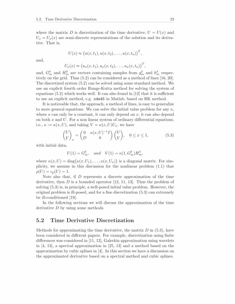
where γ = Ts/ηL2. In the numerical experiment we computed, γ ≈ 0.587,where L = 55mm, Ts = 917 x 10 sec. and η ≈ 5.164, the density ρ and thespecific heat cp of the steel are fairly constant, i.e. η, in the temperaturerange that is considered [31]. But the thermal conductivity is treated asnonlinear, κ = κ(u), is represented by the figure 7.2. In the following sec-tion we will solve the sideways heat equation for the model-1 to investigateour approach, by comparing the computing result with known temperatureTC2. If it is sufficiently stable, then we will treat model-2 by applying sametechnique for determining the temperature at x = 0.

7.2 Numerical Experiments

In the numerical experiment we used industrial data TC1, TC2 and TC3which contain temperature histories recorded at a distance L1 = 55mm,L2 = 110mm and L3 = 165mm from the surface at x = 0. Each vectorcontains 917 data elements, and the total time period was approximately2.55 minutes. Since these data vector was measured by measurement device,they would normally have some noise. Thus we smoothed each of them, andexamined the ill-posedness of the solution by using both the industrial andthe smoothed data vectors . Both types of data vectors are represented bythe figure 7.3.

Model-1: The numerical implementation of model-1 was constructed insuch way that we first solved a well-posed boundary value problem for the

7.2. Numerical Experiments 41

0 200 400 600 800 1000 1200 140025

30

35

40

45

50

55

60

65

70

Temperature [ 0C]

The

rmal

con

duct

ivity

[ W

/m 0 C

]

Figure 7.2: The thermal conductivity function κ(x, u) of the steel materialvary with temperature.

closed interval [110, 165] mm, and then we treated the Cauchy problem toreconstruct the temperature TC2 at L2 = 110mm by computing Cauchydata [u, ux] from Lx = 157mm. More precisely, we used industrial datavectors TC2 and TC3 as boundary conditions, which are the functions oft. According to the problem requirements we computed the initial steadystate temperature u0. By using u0 and boundary value-vectors we solvedwell-posed problem (7.1) for the model-1. We already described two differ-ent implicit methods for solving well-posed problems, but in the numericalexperiment we perfered ode23s to get better accuracy. During the compu-tation it is required to supply discretized grids for the space domain, whichwas executed by using finite difference method. At the same time, we hadto take care the boundary values as well. They were evaluated in each timestep by linear interpolation. We have discussed in detail, the solving pro-cedure of a well-posed problem, in chapter 6. We computed the heat fluxux(x, ·) by using the formula,

ux = (u(x + hx) − u(x − hx))/2hx,

where hx = 1/(N+1) is the step size in the x-direction. we selected N = 100inner points.

Before the inverse problem was solved by using Cauchy data [u, ux],we interpolated them into an equidistant grid tknk=0 of size n = 918.Finally, the space marching was performed using Matlab routine ode45 withautomatic step size control, a Runge-Kutta-Fehlberg method is of order 5.

42 Chapter 7. An Experiment for an Industrial Application

0 0.1 0.2 0.3 0.4 0.5 0.6 0.7 0.8 0.9 10

200

400

600

800

1000

1200

1400

Time [s]

Tem

pera

ture

[ 0 C

]

TC1TC2TC3

0 0.1 0.2 0.3 0.4 0.5 0.6 0.7 0.8 0.9 10

200

400

600

800

1000

1200

1400

Time [s]

Tem

pera

ture

[ 0 C

]

TC1TC2TC3

Figure 7.3: Industrial measured temperature TC1, TC2 and TC3 for steelmaterial are described by the top figure, which are non-smooth data vectors,i.e. they contain some noise by the measurement device when they weremeasured. A smooth version of the same data vectors can be illustrated bythe bottom figure.

7.2. Numerical Experiments 43

During the space marching we needed to compute the time derivative ∂∂t .

We used spline function for approximating the derivative, cf. section 5.2.2.In that case we selected a set of coarse grids βj with grid parameter ∆β,which act individually as a break point for approximating the derivative. Inthe experiment for model-1 we used different grid parameter ∆β for bothnon-smooth and smooth cases. The regularizing effects of different gridparameter can be observed by the figures 7.5 and 7.7 respectively. Thegraphical results for the numerical tests look quite good.

Model-2: Here the case is different from model-1 since we have no in-formation about the desired temperature at x = 0. Thus, in this case, wefollowed the numerical techniques and procedures of model-1, but we didsome more experiments by taking different length of industrial data vec-tors for both non-smooth and smooth cases. In order to find the solutiontemperature TC0 at x = 0 we had to solve a well-posed boundary valueproblem for the closed interval [55, 110] mm, and then we evaluated heatflux at x = 55mm. Since we had Cauchy data [u, ux] at x = 55mm, wesolved the sideways heat equation for the interval [55, 0] mm, i.e. [1, 0] forthe scaled version, by using these data vectors with two different tests.

Test 1: In the first test, for solving the inverse problem we interpolatedthe Cauchy data into an equidistant grid tknk=0 of size n = 918. Duringthe space marching we computed the time derivative ∂

∂t by using splinefunction, where we selected a coarse grid βj with different grid parameter,i.e. ∆β = 1/5, 1/10, 1/20, 1/30 ,1/100 and 1/180, which act individuallyas a break point for approximating the derivative. The regularizing effectsfor both non-smooth and smooth cases with different grid parameter can beobserved by the figures 7.10 and 7.11 respectively. Since the industrial data(non-smooth) is noisy we can easily see the ill-posedness of the solutions fordifferent grid parameter in figure 7.10. Whereas, we have good results forsmooth data in figure 7.11.

Test 2: Finally we solved the inverse problem by interpolating theCauchy data into an equidistant grid tknk=0 of size n = 400. For approx-imating the time derivative we applied the same grid parameters which weused for Test 1. The regularizing effects for both non-smooth and smoothcases can be seen by the figures 7.13 and 7.14 respectively. Since we selecteda small length of industrial data, i.e. 400 for both non-smooth and smoothvectors, we found less ill-posedness in the solution using different grid pa-rameter. We found good results for smooth data in figure 7.14 compared tonon-smooth data in figure 7.13.

44 Chapter 7. An Experiment for an Industrial Application

0 0.1 0.2 0.3 0.4 0.5 0.6 0.7 0.8 0.9 10

200

400

600

800

1000

1200

1400

gmnon−smooth

0 0.1 0.2 0.3 0.4 0.5 0.6 0.7 0.8 0.9 10

200

400

600

800

1000

1200

1400

Time [s]

Tem

pera

ture

[ 0 C

]

measured temperature g(t) at x=157mm

gmsmooth

0 0.1 0.2 0.3 0.4 0.5 0.6 0.7 0.8 0.9 1−200

−150

−100

−50

0

50

100

150

200

hmnon−smooth

0 0.1 0.2 0.3 0.4 0.5 0.6 0.7 0.8 0.9 1−200

−150

−100

−50

0

50

100

150

200

Time [s]

Tem

pera

ture

[ 0 C

]

measured heat flux h(t) at x=157mm

hmsmooth

Figure 7.4: The temperature vectors g(t) = u(157mm, t) were obtainedby solving a well-posed boundary value problem for model-1 by using bothnon-smooth and smooth vectors respectively showing by the top pair of thisfigure. Heat flux h(t) for both non-smooth and smooth data vectors wereevaluated at Lx = 157mm showing by the bottom pair respectively. Forboth cases we used industrial data vectors as a length 918.

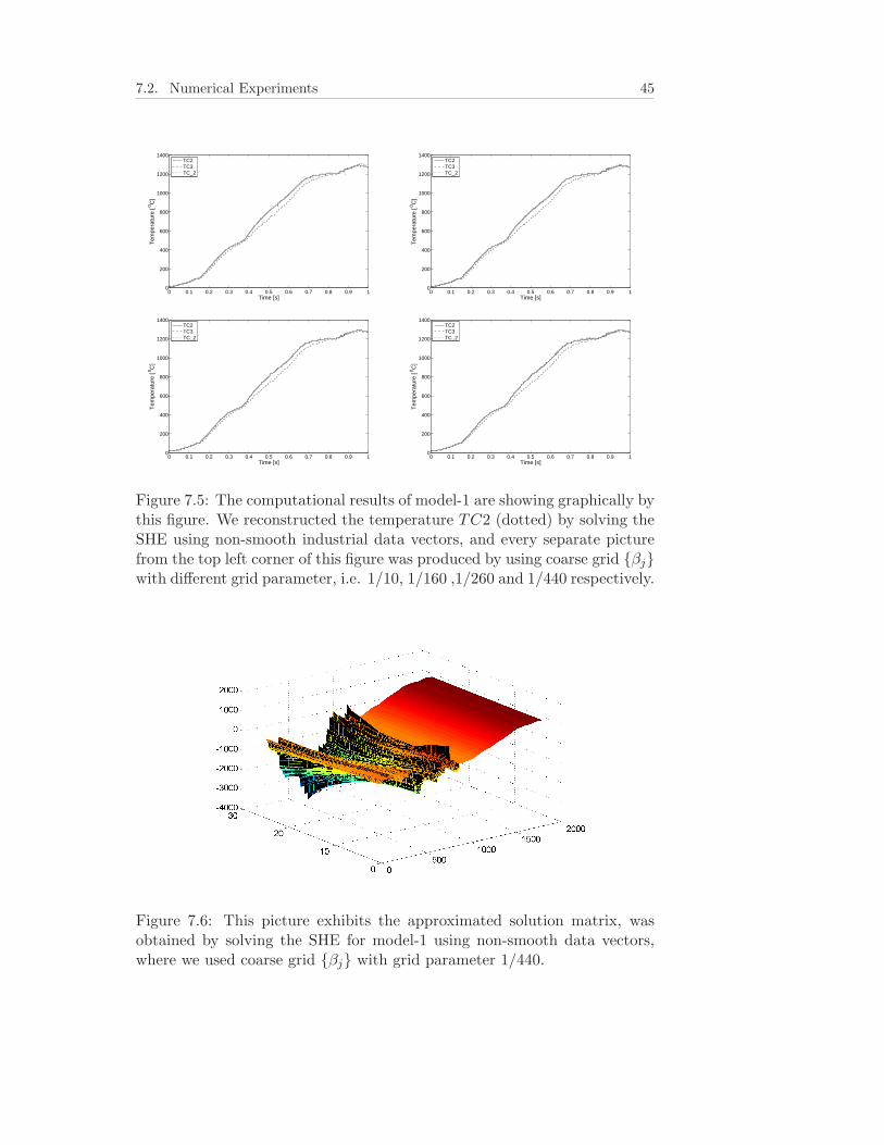
7.2. Numerical Experiments 45

0 0.1 0.2 0.3 0.4 0.5 0.6 0.7 0.8 0.9 10

200

400

600

800

1000

1200

1400

Time [s]

Tem

pera

ture

[ 0 C

]

TC2TC3TC_2

0 0.1 0.2 0.3 0.4 0.5 0.6 0.7 0.8 0.9 10

200

400

600

800

1000

1200

1400

Time [s]

Tem

pera

ture

[ 0 C

]

TC2TC3TC_2

0 0.1 0.2 0.3 0.4 0.5 0.6 0.7 0.8 0.9 10

200

400

600

800

1000

1200

1400

Time [s]

Tem

pera

ture

[ 0 C

]

TC2TC3TC_2

0 0.1 0.2 0.3 0.4 0.5 0.6 0.7 0.8 0.9 10

200

400

600

800

1000

1200

1400

Time [s]

Tem

pera

ture

[ 0 C

]

TC2TC3TC_2

Figure 7.5: The computational results of model-1 are showing graphically bythis figure. We reconstructed the temperature TC2 (dotted) by solving theSHE using non-smooth industrial data vectors, and every separate picturefrom the top left corner of this figure was produced by using coarse grid βjwith different grid parameter, i.e. 1/10, 1/160 ,1/260 and 1/440 respectively.

Figure 7.6: This picture exhibits the approximated solution matrix, wasobtained by solving the SHE for model-1 using non-smooth data vectors,where we used coarse grid βj with grid parameter 1/440.

46 Chapter 7. An Experiment for an Industrial Application

0 0.1 0.2 0.3 0.4 0.5 0.6 0.7 0.8 0.9 10

200

400

600

800

1000

1200

1400

Time [s]

Tem

pera

ture

[ 0 C

]

TC2TC3TC_2

0 0.1 0.2 0.3 0.4 0.5 0.6 0.7 0.8 0.9 10

200

400

600

800

1000

1200

1400

Time [s]

Tem

pera

ture

[ 0 C

]

TC2TC3TC_2

0 0.1 0.2 0.3 0.4 0.5 0.6 0.7 0.8 0.9 10

200

400

600

800

1000

1200

1400

Time [s]

Tem

pera

ture

[ 0 C

]

TC2TC3TC_2

0 0.1 0.2 0.3 0.4 0.5 0.6 0.7 0.8 0.9 10

200

400

600

800

1000

1200

1400

Time [s]

Tem

pera

ture

[ 0 C

]

TC2TC3TC_2

Figure 7.7: A graphical representation of computational results of model-1 isshowing by this figure for smooth industrial data vectors. We reconstructedthe temperature TC2 (dotted) by solving the SHE for coarse grid βj withdifferent grid parameter, i.e. 1/10, 1/30 ,1/40 and 1/230, which produceddifferent picture from the top left corner respectively.

Figure 7.8: This picture exhibits the approximated solution matrix, wasobtained by solving the SHE for model-1 using smooth data vectors, wherewe used coarse grid βj with grid parameter 1/230.

7.2. Numerical Experiments 47

0 0.1 0.2 0.3 0.4 0.5 0.6 0.7 0.8 0.9 10

500

1000

1500

gmnon−smooth

0 0.1 0.2 0.3 0.4 0.5 0.6 0.7 0.8 0.9 10

500

1000

1500

Time [s]

Tem

pera

ture

[ 0 C

]

measured temperature g(t) at x = 55mm

gmsmooth

0 0.1 0.2 0.3 0.4 0.5 0.6 0.7 0.8 0.9 1

−200

0

200

400

600

hmnon−smooth

0 0.1 0.2 0.3 0.4 0.5 0.6 0.7 0.8 0.9 1−200

0

200

400

600

Time [s]

Tem

pera

ture

[ 0 C

]

measured temperature h(t) at x = 55mm

hmsmooth

Figure 7.9: The pictures showing by the top pair in this figure are thetemperature vectors g(t) = u(55mm, t), were obtained by solving a well-posed boundary value problem for the model-2 for both non-smooth andsmooth cases respectively, and the heat flux h(t), bottom pair for bothcases, were evaluated at Lx = 55mm respectively. In both cases we usedindustrial data vectors as a length 918.

48 Chapter 7. An Experiment for an Industrial Application

0 0.1 0.2 0.3 0.4 0.5 0.6 0.7 0.8 0.9 10

500

1000

1500

Time [s]

Tem

pera

ture

[ 0 C

]

TC0TC1TC2

0 0.1 0.2 0.3 0.4 0.5 0.6 0.7 0.8 0.9 10

500

1000

1500

Time [s]

Tem

pera

ture

[ 0 C

]

TC0TC1TC2

0 0.1 0.2 0.3 0.4 0.5 0.6 0.7 0.8 0.9 10

500

1000

1500

Time [s]

Tem

pera

ture

[ 0 C

]

TC0TC1TC2

0 0.1 0.2 0.3 0.4 0.5 0.6 0.7 0.8 0.9 10

500

1000

1500

Time [s]

Tem

pera

ture

[ 0 C

]

TC0TC1TC2

0 0.1 0.2 0.3 0.4 0.5 0.6 0.7 0.8 0.9 10

200

400

600

800

1000

1200

1400

Time [s]

Tem

pera

ture

[ 0 C

]

TC0TC1TC2

0 0.1 0.2 0.3 0.4 0.5 0.6 0.7 0.8 0.9 10

200

400

600

800

1000

1200

1400

1600

Time [s]

Tem

pera

ture

[ 0 C

]

TC0TC1TC2

Figure 7.10: A graphical representation of the computational results ofmodel-2 is showing by this figure. We obtained solution temperature TC0by solving the SHE for non-smooth industrial data vectors. We used coarsegrid βj with different grid parameter, i.e. ∆β = 1/5, 1/10, 1/20, 1/30,1/100 and 1/180, which produced separate picture from the top left cornerrespectively.

7.2. Numerical Experiments 49

0 0.1 0.2 0.3 0.4 0.5 0.6 0.7 0.8 0.9 10

200

400

600

800

1000

1200

1400

Time [s]

Tem

pera

ture

[ 0 C

]

TC0TC1TC2

0 0.1 0.2 0.3 0.4 0.5 0.6 0.7 0.8 0.9 10

200

400

600

800

1000

1200

1400

Time [s]

Tem

pera

ture

[ 0 C

]

TC0TC1TC2

0 0.1 0.2 0.3 0.4 0.5 0.6 0.7 0.8 0.9 10

200

400

600

800

1000

1200

1400

Time [s]

Tem

pera

ture

[ 0 C

]

TC0TC1TC2

0 0.1 0.2 0.3 0.4 0.5 0.6 0.7 0.8 0.9 10

200

400

600

800

1000

1200

1400

Time [s]

Tem

pera

ture

[ 0 C

]

TC0TC1TC2

0 0.1 0.2 0.3 0.4 0.5 0.6 0.7 0.8 0.9 10

200

400

600

800

1000

1200

1400

Time [s]

Tem

pera

ture

[ 0 C

]

TC0TC1TC2

0 0.1 0.2 0.3 0.4 0.5 0.6 0.7 0.8 0.9 10

200

400

600

800

1000

1200

1400

Time [s]

Tem

pera

ture

[ 0 C

]

TC0TC1TC2

Figure 7.11: In the case of smooth data vectors for model-2, we found so-lution temperature TC0 by solving the SHE for coarse grid βj with eachdifferent parameter, i.e. ∆β = 1/5, 1/10, 1/20, 1/30 ,1/100 and 1/180, andin each case they produced different picture from the top left corner of thisfigure respectively.

50 Chapter 7. An Experiment for an Industrial Application

0 0.1 0.2 0.3 0.4 0.5 0.6 0.7 0.8 0.9 10

500

1000

1500

gmnon−smooth

0 0.1 0.2 0.3 0.4 0.5 0.6 0.7 0.8 0.9 10

500

1000

1500

Time [s]

Tem

pera

ture

[ 0 C

]

measured temperature g(t) at x = 55mm

gmsmooth

0 0.1 0.2 0.3 0.4 0.5 0.6 0.7 0.8 0.9 1

−200

−100

0

100

200

300

hmnon−smooth

0 0.1 0.2 0.3 0.4 0.5 0.6 0.7 0.8 0.9 1

−200

−100

0

100

200

Time [s]

Tem

pera

ture

[ 0 C

]

measured temperature h(t) at x = 55mm

hmsmooth

Figure 7.12: The temperature vectors g(t) = u(55mm, t), the top pair pic-tures of this figure, were obtained by solving a well-posed boundary valueproblem of model-2 for both non-smooth and smooth cases respectively,where the heat flux h(t), bottom pair for both cases, were evaluated atLx = 55mm respectively. For both cases we used industrial data vectors asa length 400.

7.2. Numerical Experiments 51

0 0.1 0.2 0.3 0.4 0.5 0.6 0.7 0.8 0.9 10

500

1000

1500

Time [s]

Tem

pera

ture

[ 0 C

]

TC0TC1TC2

0 0.1 0.2 0.3 0.4 0.5 0.6 0.7 0.8 0.9 10

500

1000

1500

Time [s]

Tem

pera

ture

[ 0 C

]

TC0TC1TC2

0 0.1 0.2 0.3 0.4 0.5 0.6 0.7 0.8 0.9 10

500

1000

1500

Time [s]

Tem

pera

ture

[ 0 C

]

TC0TC1TC2

0 0.1 0.2 0.3 0.4 0.5 0.6 0.7 0.8 0.9 10

500

1000

1500

Time [s]

Tem

pera

ture

[ 0 C

]

TC0TC1TC2

0 0.1 0.2 0.3 0.4 0.5 0.6 0.7 0.8 0.9 10

200

400

600

800

1000

1200

1400

Time [s]

Tem

pera

ture

[ 0 C

]

TC0TC1TC2

0 0.1 0.2 0.3 0.4 0.5 0.6 0.7 0.8 0.9 10

200

400

600

800

1000

1200

1400

1600

Time [s]

Tem

pera

ture

[ 0 C

]

TC0TC1TC2

Figure 7.13: A graphical representation of the computational results ofmodel-2 is showing by this figure. We obtained solution temperature TC0by solving the SHE for non-smooth industrial data vectors. We used coarsegrid βj with different grid parameter, i.e. ∆β = 1/5, 1/10, 1/20, 1/30,1/100 and 1/180, which produced separate picture from the top left cornerrespectively.

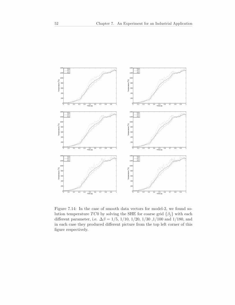
52 Chapter 7. An Experiment for an Industrial Application

0 0.1 0.2 0.3 0.4 0.5 0.6 0.7 0.8 0.9 10

200

400

600

800

1000

1200

1400

Time [s]

Tem

pera

ture

[ 0 C

]

TC0TC1TC2

0 0.1 0.2 0.3 0.4 0.5 0.6 0.7 0.8 0.9 10

200

400

600

800

1000

1200

1400

Time [s]

Tem

pera

ture

[ 0 C

]

TC0TC1TC2

0 0.1 0.2 0.3 0.4 0.5 0.6 0.7 0.8 0.9 10

200

400

600

800

1000

1200

1400

Time [s]

Tem

pera

ture

[ 0 C

]

TC0TC1TC2

0 0.1 0.2 0.3 0.4 0.5 0.6 0.7 0.8 0.9 10

200

400

600

800

1000

1200

1400

Time [s]

Tem

pera

ture

[ 0 C

]

TC0TC1TC2

0 0.1 0.2 0.3 0.4 0.5 0.6 0.7 0.8 0.9 10

200

400

600

800

1000

1200

1400

Time [s]

Tem

pera

ture

[ 0 C

]

TC0TC1TC2

0 0.1 0.2 0.3 0.4 0.5 0.6 0.7 0.8 0.9 10

200

400

600

800

1000

1200

1400

Time [s]

Tem

pera

ture

[ 0 C

]

TC0TC1TC2

Figure 7.14: In the case of smooth data vectors for model-2, we found so-lution temperature TC0 by solving the SHE for coarse grid βj with eachdifferent parameter, i.e. ∆β = 1/5, 1/10, 1/20, 1/30 ,1/100 and 1/180, andin each case they produced different picture from the top left corner of thisfigure respectively.

Chapter 8

Concluding Remarks

For the nonlinear Inverse Heat Conduction Problem (1.1) we described amathematical model for the sideways heat equation in section 1, where thesurface temperature is determined from recorded temperature which is mea-sured by a measurement device, see figure 1.1. In our numerical experimentwe have used such measured temperature from an industrial application.We have investigated the properties of the sideways heat equation by solv-ing an ill-posed Cauchy problem with Cauchy data [u, ux], and found thatit is severely ill-posed. Since the industrial data were measured by mea-surement device, they contain much noise in the data, which can be seenby the graphical results in section 7.2. Though we illustrated two differentmethods for approximating the time derivative, we used spline function, forbetter accuracy, with different grid parameter ∆β. The regularizing effectsof these grid parameters can be seen in the same section.

In order to find a right approach for solving the SHE, e.g. model-2 wefirst applied all methods and techniques for solving the SHE for model-1.By reconstructing the temperature TC2 we examined that our approachfor model-1 works well, see the graphical results in section 7.2. Since, inour experiment, the industrial data was much noisy we evaluated a smoothversion of the industrial data to reduce the noise level and used these datavectors for solving the sideways heat equation for both models to ensurethat our approach is suitable and convenient, which can be noticed by thegraphical results. By the resulting effects of both non-smooth and smoothdata we can also compare the ill-posedness by the figures, see the previoussection. It is also noticeable that if we use small length of the industrialdata vectors for the Cauchy data [u, ux], simply by interpolating them intoan equidistant grid points, we can find the problem less ill-posed. The rea-son is that, during the interpolation, the heat flux vector ux fails to picksome components which normally provide high oscillations in the solution.Thus if we take reasonably a good length, e.g. 918 components for eachof the data vectors, we can easily see the ill-posedness of the problem by

Hussain, 2010. 53

54 Chapter 8. Concluding Remarks

graphical representation of the solution. Therefore the exact ill-posednessof the problem might be seen in the solution by using the original indus-trial vectors without modifying them, and by applying an appropriate gridparameter during the regularization.

It is also remarkable that the ill-posedness is treated by approximatingthe derivative ∂

∂t by a bounded operator D. For this case we compute thederivatives of discrete functions, by approximating the function by a linearcombination B-spline basis functions, in the least squares sense, and insteadcomputing the derivative of the spline function. Moreover, the norm of thebounded operator D depends on N , the number of B-spline basis functionsthat are used. Nevertheless, we have no explicit bound for the norm, andagainst the numerical experiment we do not have a theoretical error estimate,or a formula for evaluating an appropriate value for the parameter N [4].

In general, the inverse heat conduction problem is severely ill-posed inthe sense that the solution does not depend continuously on the data. Thecase was discussed throughout this paper by giving both theoretical descrip-tion as well as numerical analysis with graphical results. Although our mainpurpose is to solve the SHE for a nonlinear problem, but for simplicity weassume all coefficients are temperature independent for the theoretical part.Moreover, to get rid of some complexity of nonlinearity we avoid such analyt-ical part in discussion. Thus several details of the numerical implementationare not completely worked out, the computational experiments demonstratethat the proposed numerical method works well.

Our approach for the objective “Numerical Solution of a Nonlinear In-verse Heat Conduction Problem” is evaluated by all the methods and numer-ical techniques we have applied, and consequently by the graphical results.The solution is reasonably good, and from this numerical experiment weexpect that the investigation, we discussed, can be useful to understand themodelling problem of a real application.

Bibliography

[1] A. B. Bakushinskii and A. V. Goncharskii. Ill-posed Problem: Theoryand Applications. Kluwer, Dordrecht, 1994.

[2] J. V. Beck. Nonlinear estimation applied to the nonlinear inverse heatconduction problem. Int. J. Heat Mass Transfer, 3:703–716, 1970.

[3] J. V. Beck, B. Blackwell, and S. R. Clair. Inverse Heat Conduction.Ill-Posed Problem. Wiley, New York, 1985.

[4] F. Berntsson. Numerical Methods for Inverse Heat Conduction Prob-lems. PhD thesis, Linkoping Studies in Science and Technology, Dis-sertations No. 723, Linkoping University, Department of Mathematics,December 2001.

[5] O. R. Burggraf. An exact solution of the inverse problem in heat con-duction theory and application. Trans. ASME, Ser. C, J. heat Transfer,86:373–382, 1964.

[6] J. R. Cannon. A priori estimates for continuation of the solution of theheat equation in the space variable. Ann. Mat. Pura Appl., 65:377–388,1964.

[7] A. Carasso. Determine surface temperatures from interior observations.SIAM Journal on Applied Mathematics, 42(3):558–574, 1982.

[8] A. Carasso. Logarithmic convexity and the ”slow evolution” constraintin ill-posed initial value problems. SIAM J. MATH. ANAL., 30(3):479–496, 1999.

[9] L. Edsberg. Introduction To Computation And Modeling For Differen-tial Equations. Wiley, 2008.

[10] L. Elden. The numerical solution of a non-characteristic Cauchy prob-lem for a parabolic equation. In P. Deuflhard and E. Hairer, editors,Numerical Treatment of Inverse Problems in Differential and IntegralEquations, Proceedings of an International Workshop, Heidelberg, 1982,pages 246–268. Birkhauser, Boston, 1983.

Hussain, 2010. 55

56 Bibliography

[11] L. Elden. Numerical solution of the sideways heat equation by differenceapproximation in time. Inverse Problem, 11:913–923, 1995.

[12] L. Elden. Solving the sideways heat equation by a ’method of lines’. J.Heat Transfer, Trans. ASME, 119:406–412, 1997.

[13] L. Elden, F. Berntsson, and T. Reginska. Wavelet and Fourier meth-ods for solving the sideways heat equation. SIAM J. Sci. Comput.,21(6):2187–2205, 2000.

[14] G. B. Folland. Fourier Analysis and its Applications. Brooks/Cole,1992.

[15] B. Gustafsson. High Order Difference Methods for Time DependentPDE. Springer, Berlin, 2008.

[16] B. Gustafsson, H. O. Kreiss, and J. Oliger. Time Dependent Problemsand Difference Methods. Wiley Interscience, New York, 1995.

[17] M. Hanke H. Engl and A . Neubauer. Regularization of Inverse Prob-lems. Kluwer Academic Publishers, Dordrecht, the Netherlands, 1996.

[18] J. Hadamard. Lectures on Cauchy’s problem in linear partial differentialequations. Dover Publications, New York, 1953.

[19] P. C. Hansen. Rank-Deficient and Discrete Ill-posed Problems. Nu-merical Aspects of Linear Inversion. Society for Industrial and AppliedMathematics, Philadelphia, 1997.

[20] J. D. Lambert. Numerical Methods for ordinary Differential Systems.Wiley, 1991.

[21] C. L. Levine. Continuous data dependence, regularization, and a threelines theorem for the heat equation with data in a space like direction.Ann. Mat. Pura Appl.(IV), CXXXIV:267–286, 1983.

[22] C. F. Van Loan. Computational frameworks for the Fast Fourier Trans-form. SIAM, Philadelphia, 1992.

[23] D. A. Murio and L. Guo. A stable space marching finite differences al-gorithm for the inverse heat conduction problem with no initial filteringprocedure. Computers Math. Applic., 19(10):35–50, 1990.

[24] Z. Ranjbar. Numerical Solution of Ill-posed Cauchy Problems forParabolic Equations. PhD thesis, Linkoping Studies in Science andTechnology, Dissertations No. 1300, Linkoping University, Departmentof Mathematics, March 2010.

Bibliography 57

[25] T. Reginska. Sideways heat equation and wavelets. J. Comput. Appl.Math., 63:209–214, 1995.

[26] G. Sewell. The Numerical Solution of Ordinary and Partial DifferentialEquations. Academic Press, 1988.

[27] L. F. Shampine and M. W. Reichelt. The MATLAB ODE Suite. SIAMJournal on Scientific Computing, 18:1–22, 1997.

[28] G. Strang. Introduction to Applied Mathematics. Wellesley-CambridgePress, 1986.

[29] A. N. Tikhonov, A. V. Goncharskii, V. V. Stepanov, and A. G. Yagola.Numerical method for the solution of ill-posed problems. Kluwer, Dor-drecht, 1995.

[30] A. N. Tikhonov, A. S. Leonov, and A. G. Yagola. Nonlinear Ill-posedProblems. Chapman and Hall, London, UK, 1998.

[31] P. Wikstrom, W. Blasiak, and F. Berntsson. Estimation of the transientsurface temperature, heat flux and effective heat transfer coefficient ofa slab in an industrial reheating furnace by using an inverse method.STEEL RESEARCH INTERNATIONAL, 78(1):63–70, 2007.

[32] M. Necati Ozisik. Finite Difference Methods in Heat Transfer. CRC,1994.

58 Bibliography

LINKÖPING UNIVERSITY

ELECTRONIC PRESS

Copyright

The publishers will keep this document online on the Internet - or its possiblereplacement - for a period of 25 years from the date of publication barring excep-tional circumstances. The online availability of the document implies a permanentpermission for anyone to read, to download, to print out single copies for your ownuse and to use it unchanged for any non-commercial research and educational pur-pose. Subsequent transfers of copyright cannot revoke this permission. All otheruses of the document are conditional on the consent of the copyright owner. Thepublisher has taken technical and administrative measures to assure authenticity,security and accessibility. According to intellectual property law the author hasthe right to be mentioned when his/her work is accessed as described above and tobe protected against infringement. For additional information about the LinkopingUniversity Electronic Press and its procedures for publication and for assurance ofdocument integrity, please refer to its WWW home page: http://www.ep.liu.se/

Upphovsratt

Detta dokument halls tillgangligt pa Internet - eller dess framtida ersattare- under 25 ar fran publiceringsdatum under forutsattning att inga extraordinaraomstandigheter uppstar. Tillgang till dokumentet innebar tillstand for var och enatt lasa, ladda ner, skriva ut enstaka kopior for enskilt bruk och att anvanda detoforandrat for ickekommersiell forskning och for undervisning. Overforing av up-phovsratten vid en senare tidpunkt kan inte upphava detta tillstand. All annananvandning av dokumentet kraver upphovsmannens medgivande. For att garan-tera aktheten, sakerheten och tillgangligheten finns det losningar av teknisk ochadministrativ art. Upphovsmannens ideella ratt innefattar ratt att bli namnd somupphovsman i den omfattning som god sed kraver vid anvandning av dokumentetpa ovan beskrivna satt samt skydd mot att dokumentet andras eller presenterasi sadan form eller i sadant sammanhang som ar krankande for upphovsmannenslitterara eller konstnarliga anseende eller egenart. For ytterligare information omLinkoping University Electronic Press se forlagets hemsida http://www.ep.liu.se/

c© 2010, Muhammad Anwar Hussain

Hussain, 2010. 59