Embed Size (px)
Citation preview
VT
T T
EC
HN
OL
OG
Y 5
4
Nu
meric
al sim
ula
tion
s on
the p
erfo
rman
ce o
f wate
rbase
d fi
re...
ISBN 978-951-38-7882-5 (URL: http://www.vtt.fi/publications/index.jsp)ISSN 2242-122X (URL: http://www.vtt.fi/publications/index.jsp)
Numerical simulations on the performance of water-based fire suppression systems
This publication summarizes a three-year research project with a goal to improve and enhance the capabilities of the NIST Fire Dynamics Simulator to describe water spray dynamics, discharge of large water based fire suppression systems, gas phase cooling by water sprays, flame extinguishment, and the suppression of large complex solid fire loads. Several new features were programmed to the code related to the description of water sprays, flame extinguishment, and suppressability of solid fire loads. Significant emphasis was put on validating the model performance against experimental data. When such data was not readily found in the literature, experiments were conducted to create the data. Due to the code development and validation work, the capability of FDS to predict the performance of fire suppression systems has been significantly improved.
Numerical simulations on the performance of waterbased fire suppressions systemsJukka Vaari | Simo Hostikka | Topi Sikanen | Antti Paajanen
•VISIONS•S
CIE
NC
E•T
ECHNOLOGY•R
ES
EA
RC
HHIGHLIGHTS
54

VTT TECHNOLOGY 54
Numerical simulations on the performance of water-based fire suppression systems
Jukka Vaari, Simo Hostikka, Topi Sikanen & Antti Paajanen

ISBN 978-951-38-7882-5 (URL: http://www.vtt.fi/publications/index.jsp) ISSN 2242-122X (URL: http://www.vtt.fi/publications/index.jsp)
Copyright © VTT 2012
JULKAISIJA – UTGIVARE – PUBLISHER
VTT PL 1000 (Tekniikantie 4 A, Espoo) 02044 VTT Puh. 020 722 111, faksi 020 722 7001
VTT PB 1000 (Teknikvägen 4 A, Esbo) FI-2044 VTT Tfn +358 20 722 111, telefax +358 20 722 7001
VTT Technical Research Centre of Finland P.O. Box 1000 (Tekniikantie 4 A, Espoo) FI-02044 VTT, Finland Tel. +358 20 722 111, fax +358 20 722 7001
Technical editing Anni Repo
Kopijyvä Oy, Kuopio 2012
3
Numerical simulations on the performance of water-based fire sup-pression systems
Jukka Vaari, Simo Hostikka, Topi Sikanen & Antti Paajanen. Espoo 2012. VTT Technology 54. 144 p.
Abstract This publication summarizes a three-year research project with a goal to improve and enhance the capabilities of the NIST Fire Dynamics Simulator to describe water spray dynamics, discharge of large water based fire suppression systems, gas phase cooling by water sprays, flame extinguishment, and the suppression of large complex solid fire loads. Several new features were programmed to the code related to the description of water sprays, flame extinguishment, and suppressability of solid fire loads. Significant emphasis was put on validating the model performance against experimental data. When such data was not readily found in the literature, experiments were conducted to create the data. Due to the code development and validation work, the capability of FDS to predict the performance of fire suppression systems has been significantly improved.
Keywords FDS, water mist, spray dynamics, sprinkler activation, flame extinguish-ment, radiation attenuation, road tunnels

4
Preface This publication is the final report of the Fire Suppression RD project carried out by VTT Technical Research Centre of Finland and Tampere University of Technology during 2008 2010. The project has been a part of the Safety and Security Programme sponsored by Tekes – the Finnish Funding Agency for Technology and Innovation. Financial support for the project has been given by VTT, Marioff Corporation Oy, Rautaruukki Oyj, YIT Kiinteistötekniikka Oy, and Markku Kauriala Ltd.
The members of the project steering group were Dr. Maarit Tuomisaari of Marioff Corporation Oy (chair), Mr. Jyri Outinen of Rautaruukki Oyj, Mr. Jukka Suoja of YIT Kiinteistötekniikka Oy, Ms. Marianna Kauriala of Markku Kauriala Ltd, Mr. Pentti Saarenrinne of Tampere University of Technology, Dr. Esko Mikkola of VTT, and Mr. Pauli Velhonoja of the Finnish Transport Agency.
The project has had an intensive collaboration with the Building and Fire Research Laboratory of the National Institute of Standards and Technology, USA, and Hughes Associates, Inc., USA, who together with VTT form the core development team of the Fire Dynamics Simulator software package.
The sponsors, the steering group and the international collaborators are gratefully acknowledged for their support throughout the project.
5
Contents Abstract ........................................................................................................... 3
Preface ............................................................................................................. 4
1. Introduction ............................................................................................... 8
2. Water spray dynamics .............................................................................. 9 2.1 Introduction ........................................................................................ 9 2.2 Nozzle types and experimental techniques ........................................ 10
2.2.1 Nozzle types ............................................................................ 10 2.2.2 Direct imaging .......................................................................... 11 2.2.3 NFPA750 experiments ............................................................. 13 2.2.4 Air entrainment ........................................................................ 14
2.3 Numerical simulation of the nozzles .................................................. 15 2.3.1 Description of the dispersed phase ........................................... 15 2.3.2 Numerical integration ............................................................... 17 2.3.3 Droplet insertion ....................................................................... 18 2.3.4 Verification of the droplet momentum transfer ........................... 18 2.3.5 Nozzle modelling ..................................................................... 21
2.4 Results ............................................................................................. 23 2.4.1 Experimental DI and PDA results for LN-2 nozzle...................... 23 2.4.2 Simulation results for LN-2 ....................................................... 25 2.4.3 NFPA 750 experiments for nozzles A, B and C ......................... 27 2.4.4 Air entrainment ........................................................................ 35
3. Activation of sprinkler systems .............................................................. 38 3.1 Introduction ...................................................................................... 38 3.2 Full-scale experiments ...................................................................... 39 3.3 FDS simulations on multiple sprinkler activation ................................. 43 3.4 FDS modelling of reduced spacing .................................................... 48 3.5 Discussion ........................................................................................ 50
4. Cooling performance .............................................................................. 53 4.1 Cooling of fire plumes ....................................................................... 53
4.1.1 Sprinkler modelling .................................................................. 54
6
4.1.2 Plume cooling model ................................................................ 56 4.1.3 Effect of drop size .................................................................... 58 4.1.4 Heat release rate at sprinkler activation .................................... 59
4.2 Attenuation of thermal radiation ......................................................... 60 4.2.1 Experimental set-up ................................................................. 61 4.2.2 Data reduction ......................................................................... 63 4.2.3 Experimental results................................................................. 65 4.2.4 Simulation of radiation attenuation tests .................................... 69
5. Flame suppression.................................................................................. 75 5.1 Combustion model in FDS v.5 ........................................................... 75
5.1.1 Flame extinguishing criterion .................................................... 76 5.1.2 Analysis of the flame extinguishing criterion .............................. 77 5.1.3 Evaluation of the flame extinguishing criterion: the cup burner ... 78
5.2 Improvements to the flame extinguishing criterion .............................. 80 5.2.1 Enthalpy calculation ................................................................. 81 5.2.2 Stoichiometry ........................................................................... 81 5.2.3 Activation energy ..................................................................... 82 5.2.4 Cell surroundings ..................................................................... 82
5.3 Performance of the new flame extinguishing criterion ......................... 83 5.3.1 Flame structure ........................................................................ 84 5.3.2 Minimum extinguishing concentrations ...................................... 85 5.3.3 Sensitivity ................................................................................ 87
5.4 Full-scale applications....................................................................... 91 5.4.1 Co-flow chimney ...................................................................... 91 5.4.2 Enclosed pool fire .................................................................... 93
5.5 Limits of validity .............................................................................. 100
6. Suppressability of idle wooden pallets ................................................. 103 6.1 Pyrolysis of wood............................................................................ 103 6.2 Burning of pallet piles ..................................................................... 104
6.2.1 Simplified model for idle wooden pallets.................................. 105 6.2.2 Freely burning pallets ............................................................. 107
6.3 Water suppression .......................................................................... 112
7. Road tunnels ......................................................................................... 119 7.1 Runehamar tunnel .......................................................................... 120
7.1.1 FDS model of the tunnel ......................................................... 120 7.1.2 FDS model of the fire source .................................................. 121 7.1.3 Heat release rate measurement.............................................. 123 7.1.4 Test 1 heat release rate ......................................................... 128
7.2 San Pedro de Anes tunnel .............................................................. 129 7.2.1 FDS model of the tunnel ......................................................... 129 7.2.2 FDS model of the fire source .................................................. 130 7.2.3 FDS model of the high pressure water mist system ................. 131 7.2.4 Heat release rate ................................................................... 132

7
7.2.5 Temperatures ........................................................................ 134 7.2.6 Backlayering .......................................................................... 135
8. Summary ............................................................................................... 137
References ................................................................................................... 140

1. Introduction
8
1. Introduction
Over the past 20 years, demonstrating the suppression performance of fixed water-based fire fighting systems has been done exclusively through extensive full-scale fire testing, although tentative computational capabilities and tools for predicting the suppression system performance have existed all along. The history of traditional sprinkler technology, spanning over 150 years, has made it possible to distil the experience into design and installation rules for these systems.
Water mist systems represent a more recent development for water based fire suppression technology. The 20-year commercial history of water mist systems has seen a large number of experimental work, but no general design and installation rules have emerged. This is primarily because there are several extinguishing mechanisms for water mist, the most important being gas-phase cooling, surface wetting, and scattering and absorption of heat radiation. The relative importance of the mechanisms is difficult to quantify as it depends on the technical details of the water mist system, as well as the application.
Water mist technology is a relatively young and developing technology. As the technology matures, the applications of the technology become larger in terms of fire risk, and accordingly more complex in terms of design. Traffic tunnels currently represent the largest applications, with a few existing installations, such as the tunnel portion of the A86 road around Paris for passenger vehicles. Full-scale testing has also been carried out for tunnels where HGV trucks are allowed.
The R&D of large fire suppression systems calls for abundant resources both in terms of time and money. This may in some instances slow down the development of the technology, particularly for water mist. Experimental demonstration of the fire suppression effectiveness of these systems will be required in the future. It can be expected however that the need for full scale work can be substantially cut down by making use of state-of-the-art fire simulation software in the R&D process. Such tools are in everyday use in the field of Fire Safety Engineering. Yet, these tools have not been applied in simulating the performance of active fire suppression systems. This development is seen as evident in the near future, and indeed it is recently recognized as the top priority by the International Forum of Fire Research Directors (Grosshandler 2007).
This publication presents the main findings obtained during a three-year research project with a goal to improve and enhance the capabilities of the Fire Dynamics Simulator to describe water spray dynamics, discharge of large water based fire suppression systems, flame extinguishment, and the suppression of large complex solid fire loads.
2. Water spray dynamics
9
2. Water spray dynamics
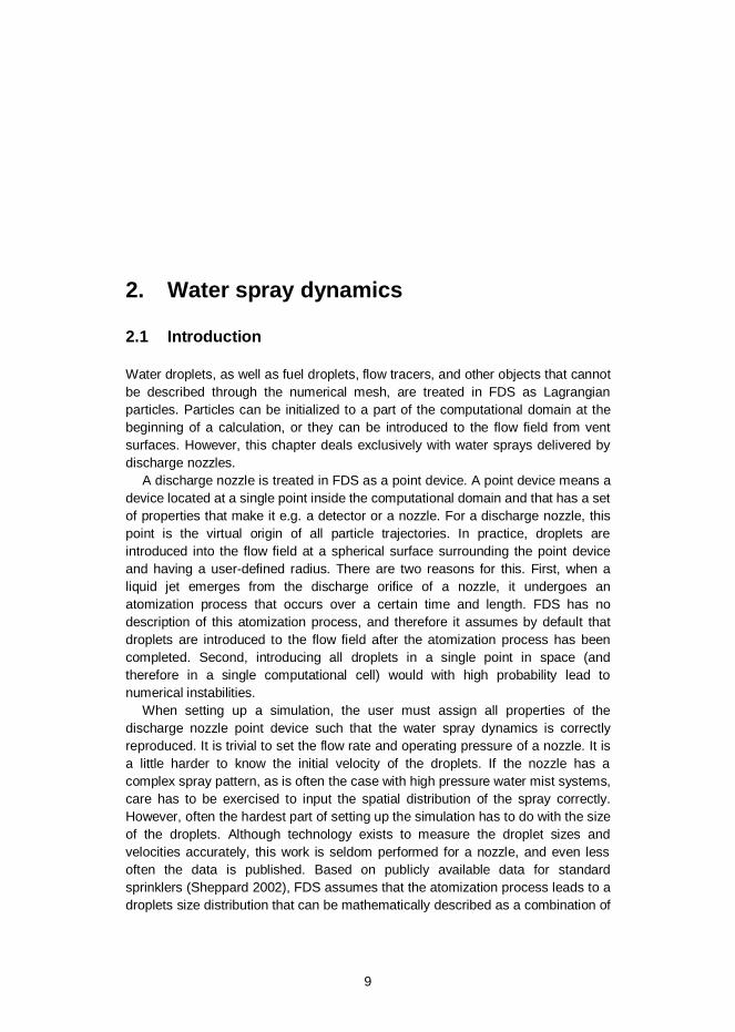
2.1 Introduction
Water droplets, as well as fuel droplets, flow tracers, and other objects that cannot be described through the numerical mesh, are treated in FDS as Lagrangian particles. Particles can be initialized to a part of the computational domain at the beginning of a calculation, or they can be introduced to the flow field from vent surfaces. However, this chapter deals exclusively with water sprays delivered by discharge nozzles.
A discharge nozzle is treated in FDS as a point device. A point device means a device located at a single point inside the computational domain and that has a set of properties that make it e.g. a detector or a nozzle. For a discharge nozzle, this point is the virtual origin of all particle trajectories. In practice, droplets are introduced into the flow field at a spherical surface surrounding the point device and having a user-defined radius. There are two reasons for this. First, when a liquid jet emerges from the discharge orifice of a nozzle, it undergoes an atomization process that occurs over a certain time and length. FDS has no description of this atomization process, and therefore it assumes by default that droplets are introduced to the flow field after the atomization process has been completed. Second, introducing all droplets in a single point in space (and therefore in a single computational cell) would with high probability lead to numerical instabilities.
When setting up a simulation, the user must assign all properties of the discharge nozzle point device such that the water spray dynamics is correctly reproduced. It is trivial to set the flow rate and operating pressure of a nozzle. It is a little harder to know the initial velocity of the droplets. If the nozzle has a complex spray pattern, as is often the case with high pressure water mist systems, care has to be exercised to input the spatial distribution of the spray correctly. However, often the hardest part of setting up the simulation has to do with the size of the droplets. Although technology exists to measure the droplet sizes and velocities accurately, this work is seldom performed for a nozzle, and even less often the data is published. Based on publicly available data for standard sprinklers (Sheppard 2002), FDS assumes that the atomization process leads to a droplets size distribution that can be mathematically described as a combination of
2. Water spray dynamics
10
log-normal and Rosin-Rammler distributions. It is up to the user to give the volume median diameter and the width parameter of this distribution.
2.2 Nozzle types and experimental techniques
2.2.1 Nozzle types
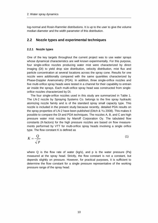
One of the key targets throughout the current project was to use water sprays whose dynamical characteristics are well known experimentally. For this purpose, four single-orifice nozzles producing water mist were characterized by direct imaging (DI) to yield drop size distribution, velocity distribution, mist flux and particle concentration at several locations across the spray cone. Results for one nozzle were additionally compared with the same quantities characterized by Phase-Doppler Anemometry (PDA). In addition, three single-orifice nozzles and five multi-orifice spray heads were tested in a channel for their capability to entrain air inside the sprays. Each multi-orifice spray head was constructed from single-orifice nozzles characterized by DI.
The four single-orifice nozzles used in this study are summarized in Table 1. The LN-2 nozzle by Spraying Systems Co. belongs to the fine spray hydraulic atomizing nozzle family and is of the standard spray small capacity type. This nozzle is included in the present study because recently, detailed PDA results on the spray properties of LN-2 have been published (Ditch & Yu 2008). This makes it possible to compare the DI and PDA techniques. The nozzles A, B, and C are high pressure water mist nozzles by Marioff Corporation Oy. The tabulated flow constants (K-factors) for the high pressure nozzles are based on flow measure-ments performed by VTT for multi-orifice spray heads involving a single orifice type. The flow constant K is defined as
pQK (1)
where Q is the flow rate of water (kg/s), and p is the water pressure (Pa) measured at the spray head. Strictly, the flow constant is not a constant, but depends slightly on pressure. However, for practical purposes, it is sufficient to determine the flow constant for a single pressure representative of the working pressure range of the spray head.
2. Water spray dynamics
11
Table 1. The single orifice nozzles.
LN-2 A B C
Type Hollow-cone Full-cone Full-cone Full-cone
Cone angle (deg)
74 30 30 30
Flow constant (kg/s/Pa1/2) (l/min/bar1/2)
4.09 10-6 0.077
1.02 10-5 0.20
2.28 10-5 0.43
4.04 10-5 0.77
Pressure (MPa)
2.0 7.0 7.0 7.0
The multi-orifice spray heads used in this study are summarized in Table 2. They are constructed by attaching single orifice nozzles of types A, B, and C (see Table 1) to a spray head body. The assembled spray head has a centre nozzle spraying in the axial direction, and a number of orifices distributed evenly at the perimeter, each spraying at an angle with respect to the axial direction.
Table 2. The multi-orifice spray heads.
SH1 SH2 SH3 SH4 SH5
Centre nozzle A C B B B
Perimeter nozzle A B A B B
Number of perimeter nozzles 6 6 8 8 8
Perimeter angle (deg) 60 60 45 45 30
2.2.2 Direct imaging
The spray measurement setup in DI measurements consists of a system for spraying and the imaging equipment. Water was pressurized with a pump and guided to the nozzle through a high pressure flexible tube. The pressure was monitored with a manometer and controlled with the unloader valve of the pump. The spray was collected below the measurement zone to a cyclone run by a fan.
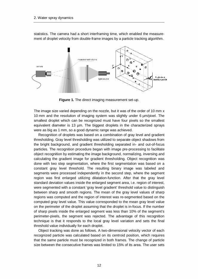
Droplets were imaged in a traditional back-light imaging system, which is illustrated in Figure 1. The camera and illumination optics were installed on a common traverse so that the scanning of different measurement positions in the spray was easy. The light source was a diode laser with a wavelength of 690 nm. The digital camera was fitted with a 200 mm lens with a 2x telecentric converter. In every measurement position typically 500 images were recorded to provide good
2. Water spray dynamics
12
statistics. The camera had a short interframing time, which enabled the measure-ment of droplet velocity from double-frame images by a particle tracking algorithm.
Figure 1. The direct imaging measurement set-up.
The image size varied depending on the nozzle, but it was of the order of 10 mm x 10 mm and the resolution of imaging system was slightly under 6 µm/pixel. The smallest droplet which can be recognized must have four pixels so the smallest equivalent diameter is 13 µm. The biggest droplets in the characterized sprays were as big as 1 mm, so a good dynamic range was achieved.
Recognition of droplets was based on a combination of gray level and gradient thresholding. Gray level thresholding was utilized to separate object shadows from the bright background, and gradient thresholding separated in- and out-of-focus particles. The recognition procedure began with image pre-processing to facilitate object recognition by estimating the image background, normalizing, inversing and calculating the gradient image for gradient thresholding. Object recognition was done with two step segmentation, where the first segmentation was based on a constant gray level threshold. The resulting binary image was labeled and segments were processed independently in the second step, where the segment region was first enlarged utilizing dilatation-function. After that the gray level standard deviation values inside the enlarged segment area, i.e. region of interest, were segmented with a constant ‘gray level gradient’ threshold value to distinguish between sharp and smooth regions. The mean of the gray level values of sharp regions was computed and the region of interest was re-segmented based on the computed gray level value. This value corresponded to the mean gray level value on the perimeter of the droplet assuming that the droplet is in-focus. If the number of sharp pixels inside the enlarged segment was less than 10% of the segment’s perimeter-pixels, the segment was rejected. The advantage of this recognition technique is that it responds to the local gray level variation and sets the final threshold value individually for each droplet.
Object tracking was done as follows. A two-dimensional velocity vector of each recognized particle was calculated based on its centroid position, which requires that the same particle must be recognized in both frames. The change of particle size between the consecutive frames was limited to 15% of its area. The user sets
2. Water spray dynamics
13
the initial guess of particle shift between the image frames and the initial guess of the radius inside of which the particle should be found, i.e. the interrogation area, in the second frame by running test analysis for a few image pairs, so that the amount of correct matches in image pairs is as high as possible. The matching of droplet pairs in the tracking algorithm was based on the smallest pseudo difference PD of size and velocity difference between the frames inside the interrogation area:
(2)
where udiff is the difference between the initial guess and real displacement, rIA is the radius of interrogation area, d1 is the diameter of the object in the first frame and d2 in the second frame. To avoid matching failures, a threshold value of pseudo difference was set to 50%.
The depth-of-field (DOF) bias is a commonly known aspect in DI. Since DOF is increasing with increasing particle size it causes the particle size distribution to be biased towards bigger particles. The DOF bias can be corrected empirically or based on optical point spread function. In this case it was done empirically as described in Putkiranta (2008). Calibrated targets were imaged at different distances from focus plane and then analyzed with the same algorithm as real spray images. As a result the DOF of certain size of particles was determined and a correction function to weigh the probability density function was defined. After analyzing a set of spray images the size of biggest recognized droplet was obtained and the depth of the measurement volume was the same as the DOF for that size of droplet. For all nozzle types the biggest droplets were between 200 µm and 1 mm. In this range the DOF where droplets were sharp enough to be recognized was 2–7 mm with an accuracy of ±250 µm. Then the size distributions were weighted to correct the number of smaller droplets inside the measurement volume.
2.2.3 NFPA750 experiments
The measurements and the calculation of gross cumulative volume (GRV) distribution were in accordance with the NFPA750 standard except that one measurement point was added in the centre of the spray, since the measured fire suppression nozzles (A, B and C) were producing a relatively narrow cone with a dense core. The NFPA750 is more intended for sprinklers with deflector plates where the spray is wide and the centre of the spray is unoccupied with droplets. If the centre point was not included, a significant amount of the mist flux would be ignored. For every nozzle type at least two individual nozzles were tested. The measurement points in the spray cross-section were located in eight directions
%1001
21
ddd
ru
PDIA
diff

2. Water spray dynamics
14
with distances 0.203D, 0.353D and 0.456D. The purpose of this procedure was to divide the cross-section into 24 equal areas, but as the centre point is added the corresponding area of the centre was subtracted from the points next to it. The GRV distribution was calculated as
)()( ,
ii
iijij VA
VARGRV
(3)
where GRVj is the cumulative volume fraction of all droplets equal or less than dj, Ri,j is the cumulative volume fraction of droplets equal or less than dj at location i, Ai is the cross-sectional area at location i and Vi is the mist flux at location i. The local mist flux was calculated from DI data as
5050 DVDVii UVolCV (4)
where Ci is the measured local concentration, VolDV50 is the volume of the volume median droplet and UDV50 is the average velocity of the volume median droplet.
2.2.4 Air entrainment
For measuring the amount of air entrained by the water sprays, two different rectangular channels were constructed of plywood. For single orifice nozzles, the channel was 1.5 m long and had a cross section of 0.15 m x 0.15 m. The nozzles were installed 0.6 m from the downwind end of the channel and they were spraying along the channel axis. The air velocity in the direction of the channel axis was measured with a hot-wire anemometer. Measurements were taken 0.45 m behind the nozzle on the channel axis.
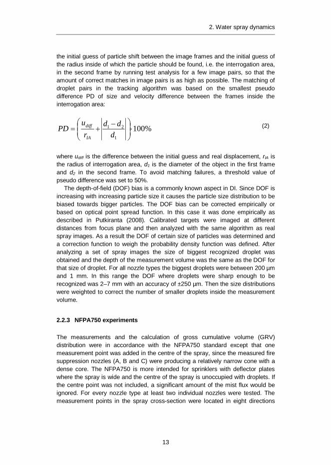
For multi-orifice spray heads, the channel was 2.0 m long and had a cross section of 0.6 m by 0.6 m. A picture of the channel with a nozzle operating is shown in Figure 2. The spray heads were installed at the midpoint of the channel and they were spraying along the channel axis. The air velocity in the direction of the channel axis was measured with a bi-directional probe. Measurements were taken 0.5 m behind the nozzle on the channel axis and 0.06 m from the channel wall. The bi-directional probe and the associated differential pressure transducer were calibrated using a hot-wire anemometer.
In each test, the water pressure was measured immediately outside the channel wall using a capacitive pressure transducer.
2. Water spray dynamics
15
Figure 2. A picture of the air entrainment measurement channel (0.6 m 0.6 m).
2.3 Numerical simulation of the nozzles
2.3.1 Description of the dispersed phase
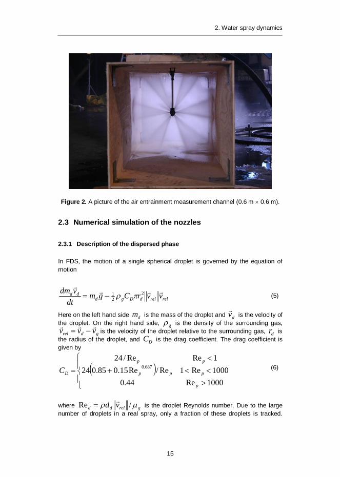
In FDS, the motion of a single spherical droplet is governed by the equation of motion
relreldDgddd vvrCgm
dtvdm 2
21 (5)
Here on the left hand side dm is the mass of the droplet and dv is the velocity of the droplet. On the right hand side, g is the density of the surrounding gas,
gdrel vvv is the velocity of the droplet relative to the surrounding gas, dr is the radius of the droplet, and DC is the drag coefficient. The drag coefficient is given by
1000Re44.01000Re1Re/Re15.085.0241ReRe/24
687.0
p
ppp
pp
DC (6)
where greldd vd /Re is the droplet Reynolds number. Due to the large number of droplets in a real spray, only a fraction of these droplets is tracked.

2. Water spray dynamics
16
Instead each droplet in the simulation represents a parcel of droplets with the same properties.
If the spray is dense enough, the individual droplets start to influence each other through aerodynamic interactions. These aerodynamic interactions may start to have an effect when the average droplet spacing is less than 10 droplet diameters. This corresponds approximately to a droplet volume fraction = 0.01. Volume fractions as high as this can sometimes be achieved inside water mist sprays.
In a configuration where two particles are directly in line, the reduction of hydrodynamic forces to the second (trailing) sphere due to the wake effect was studied by Ramírez-M noz et al. (2007). They developed the following analytical formula for the hydrodynamic force to the second sphere. In our work, this formula is used to compute a reduction factor for drag coefficient
00 F
FCC DD (7)
where CD0 is the single droplet drag coefficient and F/F0 is the hydrodynamic force ratio of trailing droplet to single droplet:
21
12
21
1
0 /1
16Reexp
/1
16Re1
dd dLdLW
FF
(8)
where Re1 is the single droplet-Reynolds number, L is the distance between the droplets and W is the non-dimensional, non-disturbed wake velocity at the centre of the trailing droplet
21
10
/1
16Reexp1
21
d
D
dLCW (9)
This model assumes that the spheres are travelling directly in-line with each other. As such, this provides an upper bound for the strength of the aerodynamic interactions. In FDS simulations, the drag reduction factor in Eq. 7 is only used, when the local droplet volume fraction exceeds 10-5. This drag reduction model is turned on by default.
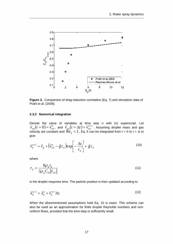
An alternative data on drag reduction was provided by Prahl et al. (2009) who studied the interaction between two solid spheres in steady or pulsating flow by detailed numerical simulations. A comparison of their results for steady inflow and the Eq. 7 is shown in Figure 3. At small drop-to-drop distances the above correlation underestimates the drag reduction significantly. The inflow pulsations were found to reduce the effect of the drag reduction. At large distances the two results are similar, the Ramírez-M noz correlation showing more drag reduction.
2. Water spray dynamics
17
Figure 3. Comparison of drag-reduction correlation (Eq. 7) and simulation data of Prahl et al. (2009).
2.3.2 Numerical integration
Denote the value of variables at time step n with (n) superscript. Letnrelrel vtv 0 , and 1n
relrel vttv . Assuming droplet mass and gas velocity are constant and 1Red , Eq. 5 can be integrated from t = 0 to t = t to give
dd
dnrelg
nd gtgvvv exp1 (10)
where
relDg
ddd vC
r3
8 (11)
is the droplet response time. The particle position is then updated according to
.11 tvxx nd
nd
nd (12)
When the aforementioned assumptions hold Eq. 10 is exact. This scheme can also be used as an approximation for finite droplet Reynolds numbers and non-uniform flows, provided that the time-step is sufficiently small.
2. Water spray dynamics
18
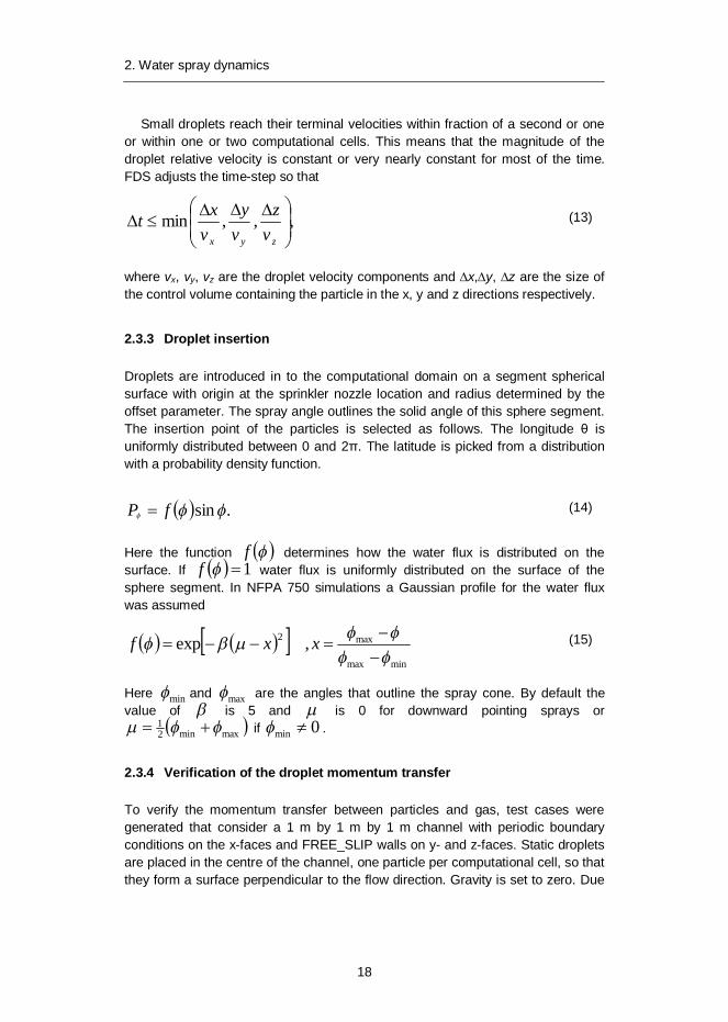
Small droplets reach their terminal velocities within fraction of a second or one or within one or two computational cells. This means that the magnitude of the droplet relative velocity is constant or very nearly constant for most of the time. FDS adjusts the time-step so that
,,,minzyx vz
vy
vxt (13)
where vx, vy, vz are the droplet velocity components and x, y, z are the size of the control volume containing the particle in the x, y and z directions respectively.
2.3.3 Droplet insertion
Droplets are introduced in to the computational domain on a segment spherical surface with origin at the sprinkler nozzle location and radius determined by the offset parameter. The spray angle outlines the solid angle of this sphere segment. The insertion point of the particles is selected as follows. The longitude is uniformly distributed between 0 and 2 . The latitude is picked from a distribution with a probability density function.
.sinfP (14)
Here the function f determines how the water flux is distributed on the surface. If 1f water flux is uniformly distributed on the surface of the sphere segment. In NFPA 750 simulations a Gaussian profile for the water flux was assumed
minmax
max2 ,exp xxf (15)
Here min and max are the angles that outline the spray cone. By default the value of is 5 and is 0 for downward pointing sprays or
maxmin21 if 0min .
2.3.4 Verification of the droplet momentum transfer
To verify the momentum transfer between particles and gas, test cases were generated that consider a 1 m by 1 m by 1 m channel with periodic boundary conditions on the x-faces and FREE_SLIP walls on y- and z-faces. Static droplets are placed in the centre of the channel, one particle per computational cell, so that they form a surface perpendicular to the flow direction. Gravity is set to zero. Due
2. Water spray dynamics
19
to the symmetry of the problem the flow is one dimensional. Assuming that the droplets are of uniform diameter and the drag coefficient and gas density are constant, the velocity in the channel decays according to
VrCB
tBuuu dD
2
0
0
21 ;
1 (16)
where V is the volume of the channel, rd is the droplet radius and u is the gas velocity in the x-direction. The summation is over all N particles. The common parameters used in all the simulations are: CD = 10, rd = 0.005 m.
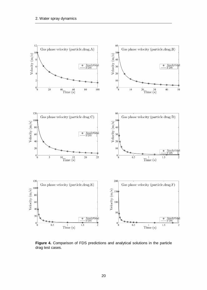
The initial velocity, u0, for each case is listed in Table 3. Comparisons of computed and analytical results are shown in Figure 4, indicating that the current integration scheme accurately predicts the amount of momentum transferred from droplets to gas phase.
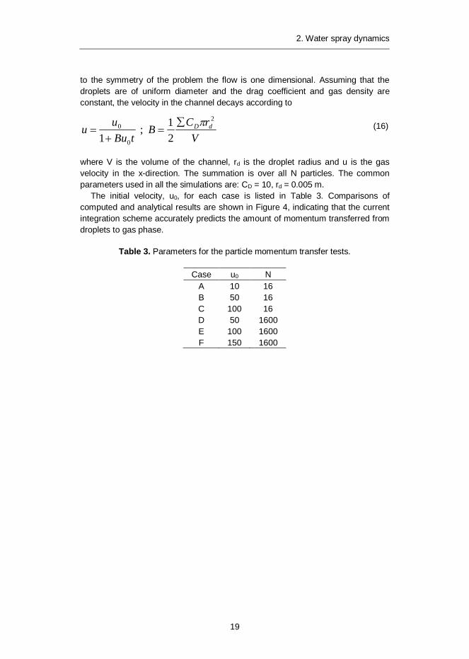
Table 3. Parameters for the particle momentum transfer tests.
Case u0 N A 10 16 B 50 16 C 100 16 D 50 1600 E 100 1600 F 150 1600
2. Water spray dynamics
20
Figure 4. Comparison of FDS predictions and analytical solutions in the particle drag test cases.

2. Water spray dynamics
21
2.3.5 Nozzle modelling
Water mist nozzles LN-2, A, B and C were modelled using the knowledge of their operating pressures, experimentally determined flow rates and droplet size distributions. The droplets were introduced to the simulation domain on a section of a spherical surface 0.05…0.1 meters away from the sprinkler location. The spray angle outlines a conical spray pattern relative to the south pole of the sphere centred at the sprinkler. The droplets are distributed within this belt as described in Section 2.3.3. For the NFPA tests and the radiation attenuation tests the Gaussian water flux profile was used for droplet insertion. For the larger tests an older version of the code was used where the longitude was picked from a uniform distribution. This corresponds to using a distribution function
1sinf in Equation 14. This places more water on the centre of the spray. The spray angles were determined from close-up photographs. The initial droplet velocities were calculated from
(17)
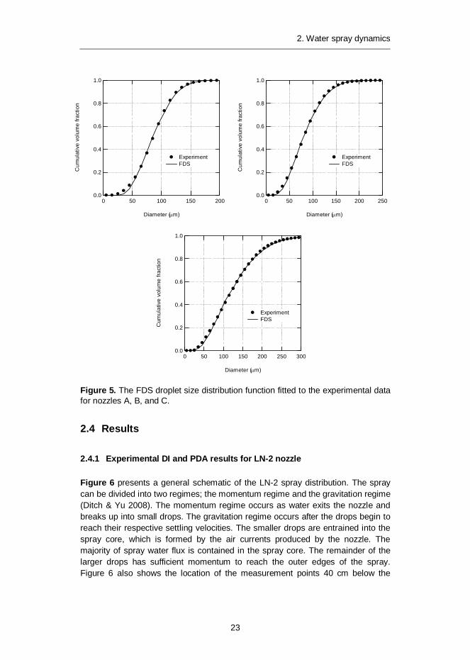
where C was taken to be 0.95 to account for friction losses in the nozzle. The droplet size distribution parameters were found by least squares fit of the mathematical form of the FDS droplet size spectrum to the experimentally determined cumulative volume distribution (Figure 5). Fitting the FDS cumulative number distribution to the experimentally measured cumulative number distribution was also tested and it was discovered that these two methods resulted in significantly different distribution parameters. In FDS, the cumulative volume fraction of droplet diameters follows a distribution that is a combination of lognormal and Rosin-Rammler distributions:
dde
ddddedF
m
m
d dd
d
mdd
m
693.00
2/ln
121
1
2
2
(18)
By default /15.1 so that the probability density function is continuous. In simulations the particle size is bounded from below by the parameter dmin. Droplets with diameters smaller than dmin are assumed to vaporize instantly. The median droplet size depends on the operating pressure used. Since the experimental droplet size distribution is determined at certain pressure this variation in droplet size is taken into account by scaling the median droplet size as
dd
PCv 20,
2. Water spray dynamics
22
31
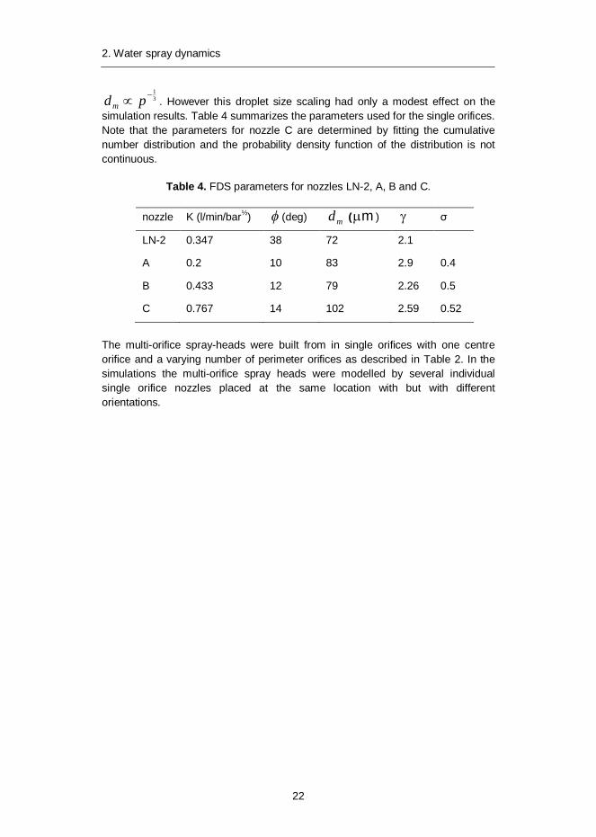
pdm . However this droplet size scaling had only a modest effect on the simulation results. Table 4 summarizes the parameters used for the single orifices. Note that the parameters for nozzle C are determined by fitting the cumulative number distribution and the probability density function of the distribution is not continuous.
Table 4. FDS parameters for nozzles LN-2, A, B and C.
nozzle K (l/min/bar½) (deg) md ( m )
LN-2 0.347 38 72 2.1
A 0.2 10 83 2.9 0.4
B 0.433 12 79 2.26 0.5
C 0.767 14 102 2.59 0.52
The multi-orifice spray-heads were built from in single orifices with one centre orifice and a varying number of perimeter orifices as described in Table 2. In the simulations the multi-orifice spray heads were modelled by several individual single orifice nozzles placed at the same location with but with different orientations.
2. Water spray dynamics
23
Figure 5. The FDS droplet size distribution function fitted to the experimental data for nozzles A, B, and C.
2.4 Results
2.4.1 Experimental DI and PDA results for LN-2 nozzle
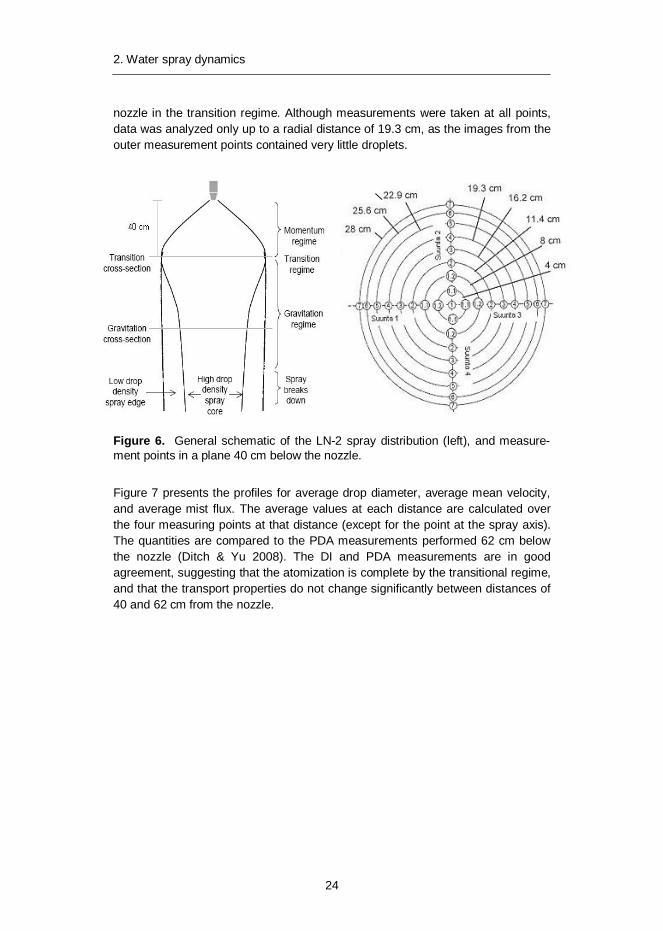
Figure 6 presents a general schematic of the LN-2 spray distribution. The spray can be divided into two regimes; the momentum regime and the gravitation regime (Ditch & Yu 2008). The momentum regime occurs as water exits the nozzle and breaks up into small drops. The gravitation regime occurs after the drops begin to reach their respective settling velocities. The smaller drops are entrained into the spray core, which is formed by the air currents produced by the nozzle. The majority of spray water flux is contained in the spray core. The remainder of the larger drops has sufficient momentum to reach the outer edges of the spray. Figure 6 also shows the location of the measurement points 40 cm below the
1.0
0.8
0.6
0.4
0.2
0.0
Cum
ulat
ive
volu
me
fract
ion
200150100500
Diameter ( m)
Experiment FDS
1.0
0.8
0.6
0.4
0.2
0.0
Cum
ulat
ive
volu
me
fract
ion
250200150100500
Diameter ( m)
Experiment FDS
1.0
0.8
0.6
0.4
0.2
0.0
Cum
ulat
ive
volu
me
fract
ion
300250200150100500
Diameter ( m)
Experiment FDS
2. Water spray dynamics
24
nozzle in the transition regime. Although measurements were taken at all points, data was analyzed only up to a radial distance of 19.3 cm, as the images from the outer measurement points contained very little droplets.
Figure 6. General schematic of the LN-2 spray distribution (left), and measure-ment points in a plane 40 cm below the nozzle.
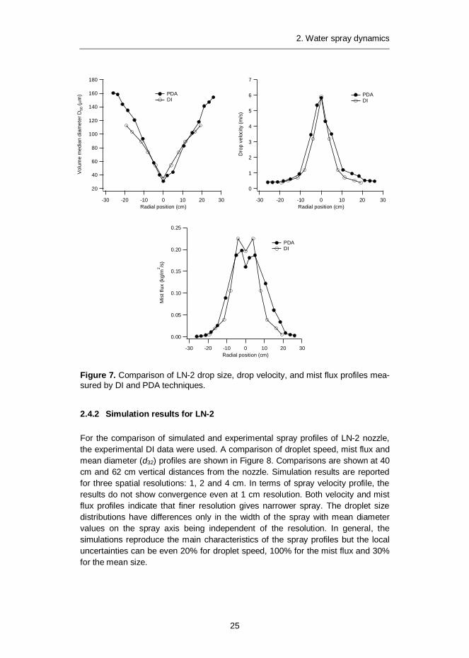
Figure 7 presents the profiles for average drop diameter, average mean velocity, and average mist flux. The average values at each distance are calculated over the four measuring points at that distance (except for the point at the spray axis). The quantities are compared to the PDA measurements performed 62 cm below the nozzle (Ditch & Yu 2008). The DI and PDA measurements are in good agreement, suggesting that the atomization is complete by the transitional regime, and that the transport properties do not change significantly between distances of 40 and 62 cm from the nozzle.
2. Water spray dynamics
25
Figure 7. Comparison of LN-2 drop size, drop velocity, and mist flux profiles mea-sured by DI and PDA techniques.
2.4.2 Simulation results for LN-2
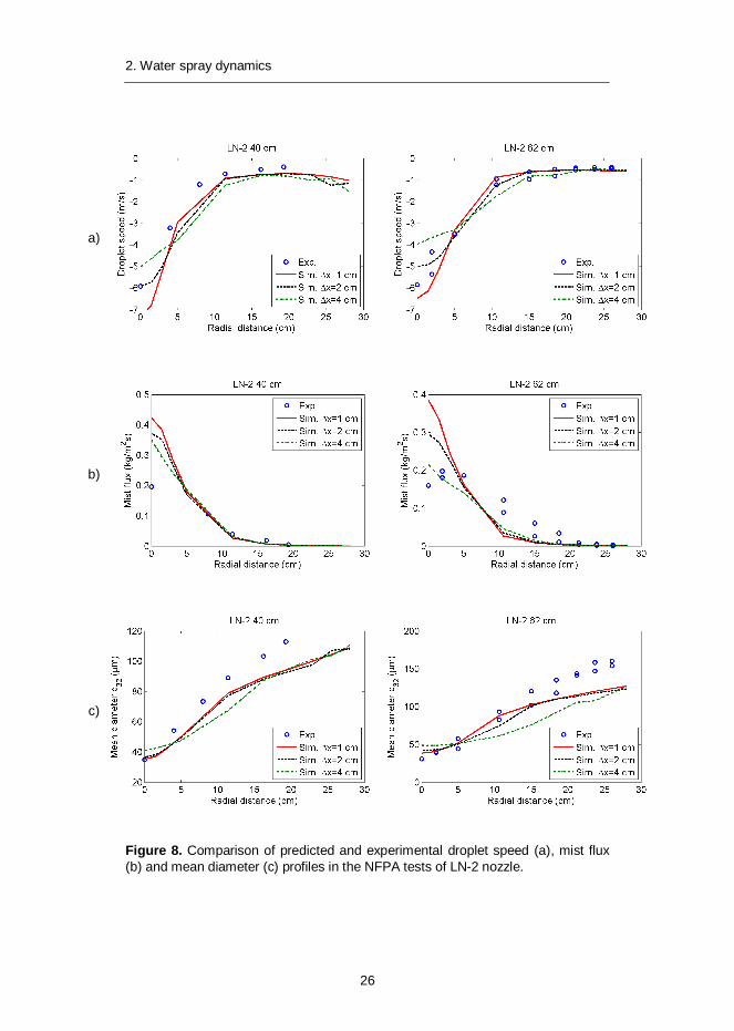
For the comparison of simulated and experimental spray profiles of LN-2 nozzle, the experimental DI data were used. A comparison of droplet speed, mist flux and mean diameter (d32) profiles are shown in Figure 8. Comparisons are shown at 40 cm and 62 cm vertical distances from the nozzle. Simulation results are reported for three spatial resolutions: 1, 2 and 4 cm. In terms of spray velocity profile, the results do not show convergence even at 1 cm resolution. Both velocity and mist flux profiles indicate that finer resolution gives narrower spray. The droplet size distributions have differences only in the width of the spray with mean diameter values on the spray axis being independent of the resolution. In general, the simulations reproduce the main characteristics of the spray profiles but the local uncertainties can be even 20% for droplet speed, 100% for the mist flux and 30% for the mean size.
180
160
140
120
100
80
60
40
20
Volu
me
med
ian
diam
eter
D50
(m
)
-30 -20 -10 0 10 20 30Radial position (cm)
PDA DI
7
6
5
4
3
2
1
0
Dro
p ve
loci
ty (m
/s)
-30 -20 -10 0 10 20 30Radial position (cm)
PDA DI
0.25
0.20
0.15
0.10
0.05
0.00
Mis
t flu
x (k
g/m
2 /s)
-30 -20 -10 0 10 20 30Radial position (cm)
PDA DI
2. Water spray dynamics
26
a)
b)
c)
Figure 8. Comparison of predicted and experimental droplet speed (a), mist flux (b) and mean diameter (c) profiles in the NFPA tests of LN-2 nozzle.
2. Water spray dynamics
27
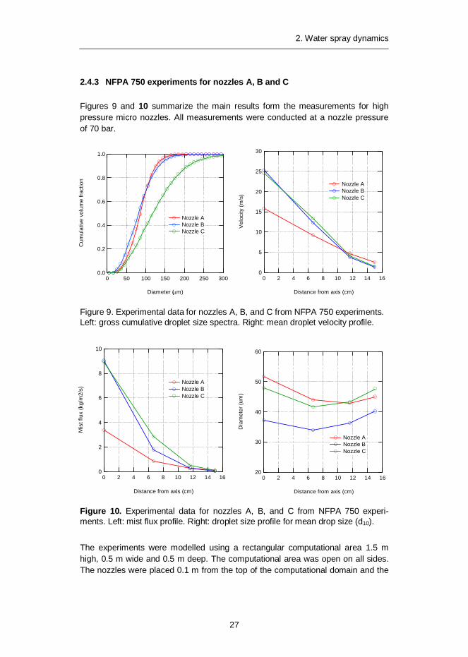
2.4.3 NFPA 750 experiments for nozzles A, B and C
Figures 9 and 10 summarize the main results form the measurements for high pressure micro nozzles. All measurements were conducted at a nozzle pressure of 70 bar.
Figure 9. Experimental data for nozzles A, B, and C from NFPA 750 experiments. Left: gross cumulative droplet size spectra. Right: mean droplet velocity profile.
Figure 10. Experimental data for nozzles A, B, and C from NFPA 750 experi-ments. Left: mist flux profile. Right: droplet size profile for mean drop size (d10).
The experiments were modelled using a rectangular computational area 1.5 m high, 0.5 m wide and 0.5 m deep. The computational area was open on all sides. The nozzles were placed 0.1 m from the top of the computational domain and the
1.0
0.8
0.6
0.4
0.2
0.0
Cum
ulat
ive
volu
me
fract
ion
300250200150100500
Diameter ( m)
Nozzle A Nozzle B Nozzle C
30
25
20
15
10
5
0
Vel
ocity
(m/s
)
1614121086420
Distance from axis (cm)
Nozzle A Nozzle B Nozzle C
10
8
6
4
2
0
Mis
t flu
x (k
g/m
2/s)
1614121086420
Distance from axis (cm)
Nozzle A Nozzle B Nozzle C
60
50
40
30
20
Dia
met
er (u
m)
1614121086420
Distance from axis (cm)
Nozzle A Nozzle B Nozzle C

2. Water spray dynamics
28
measurements are done 1 meter below the nozzle. The simulation results correspond to droplet properties averaged over a sphere with 1 cm radius centred at the measurement location.
Figure 11 shows a comparison of experimental and simulated results for mean drop velocity, mist flux and mean drop size d10.

2. Water spray dynamics
29
a)
b)
c)
Figure 11. Comparison of predicted and experimental velocity (a), mist flux (b) and average diameter (c) profiles in the NFPA tests of micro nozzles A, B and C.

2. Water spray dynamics
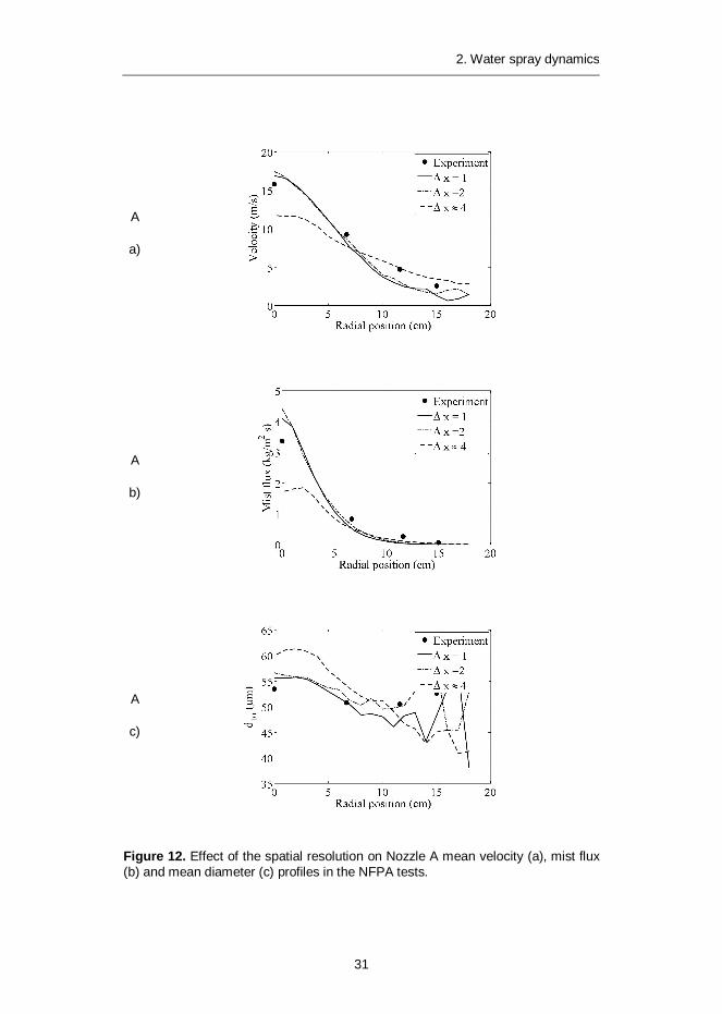
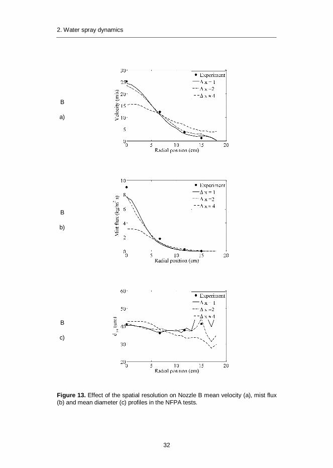
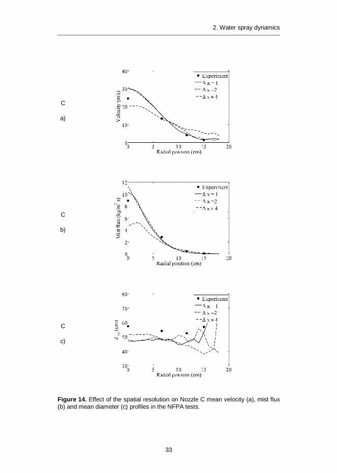
30
Spatial resolution had a strong effect on the simulation results. Discretization intervals of 1, 2 and 4 cm were investigated. Figures 12, 13 and 14 show the grid sensitivity study results for nozzles A, B and C respectively. The difference between 1 and 2 cm discretization interval was deemed insignificant, but there was a large difference between 4 cm and 2 cm grids. Coarser grids tended to flatten the distributions of velocity and mist flux. However, the diameter distribution retained its shape.
In most simulations, 105 droplets per second were used. Increasing the number of particles to 106 or 107 per second tended to yield larger velocities on the spray centreline but did not otherwise affect the results.
The minimum diameter dmin was set to 1 m in most simulations. This para-meter was sometimes increased to alleviate problems with numerical stability. Sensitivity analysis showed that this parameter did not have a noticeable effect on the results. Restricting the global time-step or increasing the number of sub-time step iterations did not improve the results either.
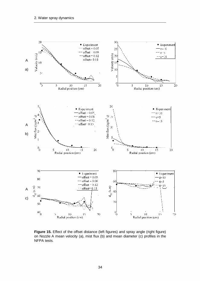
The sensitivity of the results on the initial velocity and the offset parameter was also investigated. Velocity could be varied at least 10% without a significant impact on the results. Varying the offset parameter between 5 cm and 15 cm also had negligible effect, as shown in Figure 15 for Nozzle A. The same figure also shows the impact of the spray angle.
2. Water spray dynamics
31
A
a)
A
b)
A
c)
Figure 12. Effect of the spatial resolution on Nozzle A mean velocity (a), mist flux (b) and mean diameter (c) profiles in the NFPA tests.
2. Water spray dynamics
32
B
a)
B
b)
B
c)
Figure 13. Effect of the spatial resolution on Nozzle B mean velocity (a), mist flux (b) and mean diameter (c) profiles in the NFPA tests.
2. Water spray dynamics
33
C
a)
C
b)
C
c)
Figure 14. Effect of the spatial resolution on Nozzle C mean velocity (a), mist flux (b) and mean diameter (c) profiles in the NFPA tests.
2. Water spray dynamics
34
A
a)
A
b)
A
c)
Figure 15. Effect of the offset distance (left figures) and spray angle (right figure) on Nozzle A mean velocity (a), mist flux (b) and mean diameter (c) profiles in the NFPA tests.

2. Water spray dynamics
35
The predicted diameter profile deviates somewhat from the observed. The experimental data available was for number median diameter, while only number mean could be calculated from the simulations. This difference in calculation explains some of the differences between simulations and experiment. Another source of error is the use of the FDS default size distribution instead of the experimental gross size distribution. Qualitatively the predictions are correct. A flat mean diameter profile is predicted for all the nozzles instead of the more usual V-shaped diameter profile of sprays. For nozzle C there is slight growing trend in the mean diameter as distance from the spray centreline grows.
The effect of aerodynamic interactions on water mist properties was investigated by running the nozzle characterization tests, with the aerodynamic interaction model turned on and off. The drag reduction by aerodynamic interactions had a very modest effect on the results. The most noticeable effect was the slight flattening of the droplet diameter curve. The droplet volume fractions in the densest parts of the spray are just slightly over >0.01 for all nozzles. These results indicate that droplet-droplet aerodynamic interactions are not important in modelling water mist systems. The drag reduction model was used in all simulations of this publication.
2.4.4 Air entrainment
The single nozzle experiments were modelled as a rectangular computational domain, with dimensions of the experimental channel. On the channel walls, inert solid wall boundary conditions were applied and open pressure boundaries were used for the ends of the channel. In the multi-orifice spray head experiments, the computational domain was extended outside the channel to better capture the flow pattern inside the channel. An overview of the simulation geometry is shown in Figure 16. Discretization interval was 2 cm in both the small and the large channel.
The offset parameter had a significant effect on the simulation results in both the large and the small channel. Offset value of 0.04 was used here instead of the 0.1 used for the simulation of the nozzle characterization tests. Using a too small offset value lead to unphysical results, where the flow on the channel axis behind the sprinkler was in the negative x-direction, while the sprinkler was oriented in the positive x-direction. The appropriate offset value depends on the numerical grid used: The offset should be large enough, so that the incoming droplets are distributed within more than one computational cell. In the case of multi-orifice spray heads it is also important to ensure that the grid is fine enough to resolve each of the spray jets. This becomes a problem when the orifices in the spray have orientations that are almost parallel.

2. Water spray dynamics
36
Figure 16. A picture of the simulation geometry for the larger of the air entrain-ment tests.
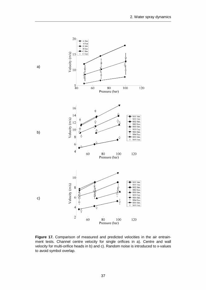
Comparisons of the air entrainment simulations to the experimental results are shown in Figure 17. Figure a) shows the centreline velocities for the single-orifice spray heads. The centreline and close-to-the-wall velocities for the multi-orifice spray-heads are shown in Figures b and c, respectively.
Of the single-orifice nozzles, the entrainment for B nozzle is predicted within the experimental uncertainty. For nozzle C the velocities in the channel are over-estimated by about 20% and for nozzle A the velocities are underestimated by similar amount. For the multi-orifice spray-heads, the agreement with experiment is good on the centreline of the channel. While the spray-heads SH4 and SH5 are both constructed from the same B type orifices, the velocities in the channel axis are slightly over predicted for SH4 and significantly under predicted for SH5. The difference between these spray-heads is in the amount of x-momentum injected in to the simulation. The SH5 spray-head has the perimeter nozzles at 30 degree angle relative to the x-axis giving the highest x-momentum of all the spray heads considered in this paper.
2. Water spray dynamics
37
a)
b)
c)
Figure 17. Comparison of measured and predicted velocities in the air entrain-ment tests. Channel centre velocity for single orifices in a). Centre and wall velocity for multi-orifice heads in b) and c). Random noise is introduced to x-values to avoid symbol overlap.
3. Activation of sprinkler systems
38
3. Activation of sprinkler systems
3.1 Introduction
The European technical specification for water mist systems, FprCEN/TS 14972:2010, gives guidance on the design and installation of these systems, and provides fire test procedures from which the main installation parameters are derived. However, the issue of hydraulic dimensioning is not fully addressed by the specification. A common practice is to adopt the hydraulic dimensioning area from the sprinkler standard EN12845.
The practice implies at least three issues of significance for water mist systems. First, the hydraulic dimensioning in EN12845 is based on the well established hazard classes of light, ordinary, and high hazards. However, the fire test procedures for water mist systems are not generic to a hazard class, but rather particular to certain groups of applications. Second, the absolute hydraulic dimensioning area must be covered despite the fact that sprinklers cannot always be installed at their maximum tested spacing. This leads to extra nozzles, and extra pumping capacity. Third, there are important differences between the properties of water sprays from standard sprinklers and water mist sprinklers, which may lead to a significantly different number of activations for the same fire between these systems.
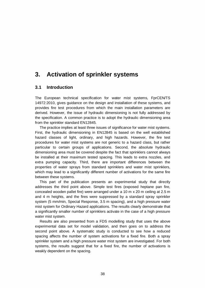
This part of the publication presents an experimental study that directly addresses the third point above. Simple test fires (exposed heptane pan fire, concealed wooden pallet fire) were arranged under a 10 m x 20 m ceiling at 2.5 m and 4 m heights, and the fires were suppressed by a standard spray sprinkler system (5 mm/min, Special Response, 3.5 m spacing), and a high pressure water mist system for Ordinary Hazard applications. The results clearly demonstrate that a significantly smaller number of sprinklers activate in the case of a high pressure water mist system.
Results are also presented from a FDS modelling study that uses the above experimental data set for model validation, and then goes on to address the second point above. A systematic study is conducted to see how a reduced spacing affects the number of system activations for a fixed fire. Both a spray sprinkler system and a high pressure water mist system are investigated. For both systems, the results suggest that for a fixed fire, the number of activations is weakly dependent on the spacing.
3. Activation of sprinkler systems
39
Based on the results of this study, it is suggested that the hydraulic dimensioning of water-based automatic fire suppression systems could be based on the number of activations observed in a fire performance test (plus a possible safety factor), and that in actual installations, the dimensioning could be based on a fixed number of sprinklers rather than an absolute dimensioning area.
3.2 Full-scale experiments
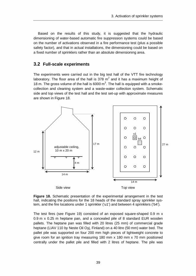
The experiments were carried out in the big test hall of the VTT fire technology laboratory. The floor area of the hall is 378 m2 and it has a maximum height of 18 m. The gross volume of the hall is 6000 m3. The hall is equipped with a smoke-collection and cleaning system and a waste-water collection system. Schematic side and top views of the test hall and the test set-up with approximate measures are shown in Figure 18.
12 m
17 m adjustable ceiling, 10 m x 20 m
4 m
Top view Side view
14 m
14 m
27 m
u1
b4
Figure 18. Schematic presentation of the experimental arrangement in the test hall, indicating the positions for the 18 heads of the standard spray sprinkler sys-tem, and the fire locations under 1 sprinkler (‘u1’) and between 4 sprinklers (‘b4’). The test fires (see Figure 19) consisted of an exposed square-shaped 0.9 m x 0.9 m x 0.25 m heptane pan, and a concealed pile of 8 standard EUR wooden pallets. The heptane pan was filled with 20 litres (25 mm) of commercial grade heptane (LIAV 110 by Neste Oil Oyj, Finland) on a 40 litre (50 mm) water bed. The pallet pile was supported on four 200 mm high pieces of lightweight concrete to give room for an ignition tray measuring 180 mm x 180 mm x 70 mm positioned centrally under the pallet pile and filled with 2 litres of heptane. The pile was
3. Activation of sprinkler systems
40
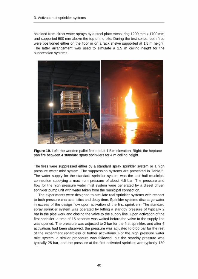
shielded from direct water sprays by a steel plate measuring 1200 mm x 1700 mm and supported 500 mm above the top of the pile. During the test series, both fires were positioned either on the floor or on a rack shelve supported at 1.5 m height. The latter arrangement was used to simulate a 2.5 m ceiling height for the suppression systems.
Figure 19. Left: the wooden pallet fire load at 1.5 m elevation. Right: the heptane pan fire between 4 standard spray sprinklers for 4 m ceiling height.
The fires were suppressed either by a standard spray sprinkler system or a high pressure water mist system. The suppression systems are presented in Table 5. The water supply for the standard sprinkler system was the test hall municipal connection supplying a maximum pressure of about 4.5 bar. The pressure and flow for the high pressure water mist system were generated by a diesel driven sprinkler pump unit with water taken from the municipal connection.
The experiments were designed to simulate real sprinkler systems with respect to both pressure characteristics and delay time. Sprinkler systems discharge water in excess of the design flow upon activation of the first sprinklers. The standard spray sprinkler system was operated by letting a standby pressure of typically 2 bar in the pipe work and closing the valve to the supply line. Upon activation of the first sprinkler, a time of 15 seconds was waited before the valve to the supply line was opened. The pressure was adjusted to 2 bar for the first sprinkler, and after 6 activations had been observed, the pressure was adjusted to 0.56 bar for the rest of the experiment regardless of further activations. For the high pressure water mist system, a similar procedure was followed, but the standby pressure was typically 25 bar, and the pressure at the first activated sprinkler was typically 130
3. Activation of sprinkler systems
41
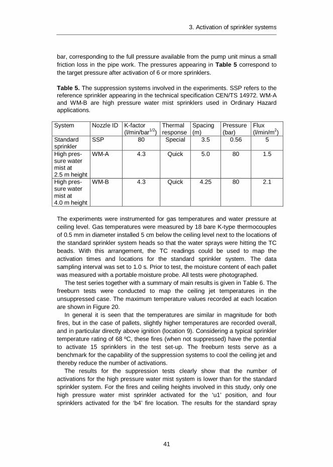
bar, corresponding to the full pressure available from the pump unit minus a small friction loss in the pipe work. The pressures appearing in Table 5 correspond to the target pressure after activation of 6 or more sprinklers.
Table 5. The suppression systems involved in the experiments. SSP refers to the reference sprinkler appearing in the technical specification CEN/TS 14972. WM-A and WM-B are high pressure water mist sprinklers used in Ordinary Hazard applications.
System Nozzle ID K-factor (l/min/bar1/2)
Thermal response
Spacing (m)
Pressure (bar)
Flux (l/min/m2)
Standard sprinkler
SSP 80 Special 3.5 0.56 5
High pres-sure water mist at 2.5 m height
WM-A 4.3 Quick 5.0 80 1.5
High pres-sure water mist at 4.0 m height
WM-B 4.3 Quick 4.25 80 2.1
The experiments were instrumented for gas temperatures and water pressure at ceiling level. Gas temperatures were measured by 18 bare K-type thermocouples of 0.5 mm in diameter installed 5 cm below the ceiling level next to the locations of the standard sprinkler system heads so that the water sprays were hitting the TC beads. With this arrangement, the TC readings could be used to map the activation times and locations for the standard sprinkler system. The data sampling interval was set to 1.0 s. Prior to test, the moisture content of each pallet was measured with a portable moisture probe. All tests were photographed.
The test series together with a summary of main results is given in Table 6. The freeburn tests were conducted to map the ceiling jet temperatures in the unsuppressed case. The maximum temperature values recorded at each location are shown in Figure 20.
In general it is seen that the temperatures are similar in magnitude for both fires, but in the case of pallets, slightly higher temperatures are recorded overall, and in particular directly above ignition (location 9). Considering a typical sprinkler temperature rating of 68 ºC, these fires (when not suppressed) have the potential to activate 15 sprinklers in the test set-up. The freeburn tests serve as a benchmark for the capability of the suppression systems to cool the ceiling jet and thereby reduce the number of activations.
The results for the suppression tests clearly show that the number of activations for the high pressure water mist system is lower than for the standard sprinkler system. For the fires and ceiling heights involved in this study, only one high pressure water mist sprinkler activated for the ‘u1’ position, and four sprinklers activated for the ‘b4’ fire location. The results for the standard spray
3. Activation of sprinkler systems
42
sprinkler system depended on the ceiling height such that more sprinklers activated in the case of 2.5 m height. The results for the 4 m ceiling height also suggest that fire location affects the number of activations such that more activations are observed for the ‘u1’ location. This is especially observed for the pallet fire load.
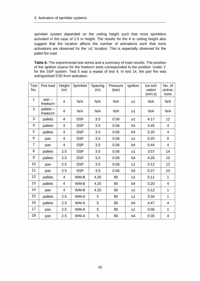
Table 6. The experimental test series and a summary of main results. The position of the ignition source for the freeburn tests corresponded to the position ‘under 1’ for the SSP system. Test 5 was a repeat of test 4. In test 14, the pan fire was extinguished 5:05 from activation.
Test No.
Fire load
Height (m)
Sprinkler
Spacing (m)
Pressure (bar)
Ignition
1st acti-vation (min:s)
No. of activa-tions
1 pan – freeburn 4 N/A N/A N/A u1 N/A N/A
2 pallets – freeburn 4 N/A N/A N/A u1 N/A N/A
3 pallets 4 SSP 3.5 0.56 u1 4:17 12 4 pallets 4 SSP 3.5 0.56 b4 4:45 4 5 pallets 4 SSP 3.5 0.56 b4 5:20 4 6 pan 4 SSP 3.5 0.56 u1 0:20 6 7 pan 4 SSP 3.5 0.56 b4 0:44 4 8 pallets 2.5 SSP 3.5 0.56 u1 3:57 14 9 pallets 2.5 SSP 3.5 0.56 b4 4:26 15
10 pan 2.5 SSP 3.5 0.56 u1 0:12 12 11 pan 2.5 SSP 3.5 0.56 b4 0:27 10 12 pallets 4 WM-B 4.25 80 u1 5:11 1 13 pallets 4 WM-B 4.25 80 b4 5:20 4 14 pan 4 WM-B 4.25 80 u1 0:12 1 15 pallets 2.5 WM-A 5 80 u1 3:34 1 16 pallets 2.5 WM-A 5 80 b4 4:47 4 17 pan 2.5 WM-A 5 80 u1 0:06 1 18 pan 2.5 WM-A 5 80 b4 0:30 4

3. Activation of sprinkler systems
43
1 2 3 4 5 6
7 8 9 10 11 12
13 14 15 16 17 18
90 79 63
104 98 80
127 111 102
115 90 87
79 68 69
51 50 58
99 80 68
143 111 113
613 333 345
131 108 108
87 73 69
55 53 58
92 77 65
105 88 85
140 113 113
109 93 84
78 69 67
47 47 55
Figure 20. Maximum ceiling jet temperatures, in degrees centigrade, in the freeburn tests. Ceiling height 4 m. The three values for each location (from the top) correspond to the pallet fire, the pan fire, and the FDS simulation for the pan fire.
3.3 FDS simulations on multiple sprinkler activation
The capability of FDS to predict the activation of multiple standard sprinklers has been demonstrated in the FDS Validation Guide for an experimental test series (Sheppard & Steppan 1997) involving heptane spray fires. In this work, selected heptane pan fires were modelled with FDS version 5.1.5 to provide further validation for sprinklers, and to extend the validation to include high pressure water mist systems. Of particular interest in this work was to investigate whether FDS can correctly predict the qualitative difference in the number of activations between the standard sprinkler system and the high pressure water mist system.
The FDS model of the test set-up is shown in Figure 21. The test hall was modelled as a rectangular volume measuring 26.0 m x 14.4 m x 16.5 m. From the floor level up to a height of 4.5 m the grid size was 10 cm, and above that the grid size was 20 cm. In total 2.2 million cells in four grids were used to model the entire volume.
Only pan fire tests were modelled in this study. A heptane pan may be fairly accurately modelled by a burner of a fixed HRR. Since heptane is a low flash-point liquid, water has little suppression effectiveness in conditions where the oxygen supply to the fire is unlimited (Kokkala 1990). A HRR value of 1.7 MW was used in this study to represent the pan fire, based on the mass loss rate data shown in Figure 22. Furthermore, the experimental ceiling jet temperatures were compared with a series of FDS simulations for a variable HRR. The best overall agreement between simulated and measured ceiling jet temperatures was obtained for a HRR of 1.7 MW (see Figure 20).
3. Activation of sprinkler systems
44
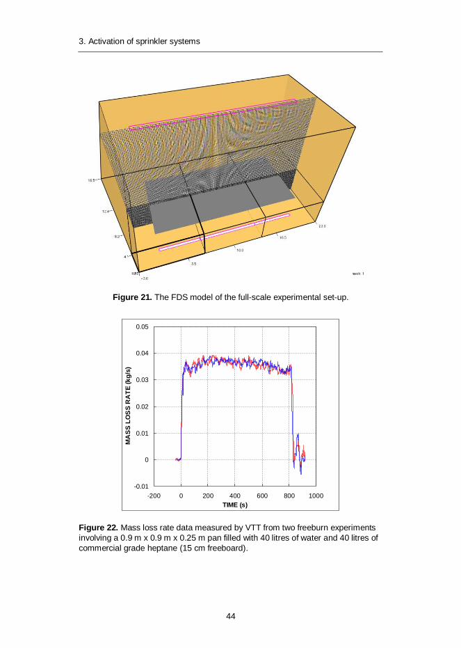
Figure 21. The FDS model of the full-scale experimental set-up.
Figure 22. Mass loss rate data measured by VTT from two freeburn experiments involving a 0.9 m x 0.9 m x 0.25 m pan filled with 40 litres of water and 40 litres of commercial grade heptane (15 cm freeboard).
-0.01
0
0.01
0.02
0.03
0.04
0.05
-200 0 200 400 600 800 1000TIME (s)
MA
SS L
OS
S R
ATE
(kg/
s)

3. Activation of sprinkler systems
45
For modelling of the sprinklers used in the simulations, approximations were necessary because detailed information on the physical properties of the water sprays (drop velocities, drop size data) was not available. The standard spray sprinklers were considered to discharge water homogeneously to angles between 50 and 80 degrees from vertical. The droplet initial velocity was set to 14 m/s at 0.1 m offset distance. The value corresponds to a pressure of 1 bar, and was a compromise choice because FDS 5.1.5 did not have the capability to change the operating pressure of sprinklers in the middle of a run. The default drop size distribution was used with the median volumetric diameter of 700 m. The spatial distribution of water sprays for the high pressure water mist sprinklers was created using the spray pattern table property of FDS to correspond to the exit angles of the micro nozzles. The initial velocity of 160 m/s at 0.02 m offset distance corresponded to a pressure of 130 bar. The default drop size distribution was used with the median volumetric diameter of 200 m.
As discussed in Chapter 2 of this publication, it is important when modelling high velocity water sprays to ensure that the momentum transfer between the droplets and the surrounding gas is fully taken into account. For reasons of numerical stability, FDS may in some instances cut off part of this momentum transfer. To ensure this would not happen, the overall time step DT and the sprinkler droplet insertion time step DT_INSERT were both limited to 0.002 s. The parameter DROPLETS_PER_SECOND was set to 50000. Finally, the particle-gas momentum transfer limiter (variable FLUXMAX) was increased from its default value of 100 to a value of 7000.
Four pan fire tests were simulated. The main results are presented in Figure 23. Overall, the number of activations is fairly accurately predicted by FDS, with only SSP 4m u1 showing two activations more than the experiment. For SSP 2.5m b4 the predicted number of activations is the same as observed in the experiment, but there is a small discrepancy in the locations. For the high pressure water mist system, both the number of activations and the locations were predicted correctly. It is pointed out that the case of a pan fire under 1 sprinkler very clearly demonstrates not only the cooling capability of high pressure water mist, but also the capability of FDS to capture this cooling effect.
The agreement between the measured and predicted activation times is less satisfactory. In general, the activation times predicted by FDS are faster than the experimentally observed activation times. For the sprinklers closest to the fire, the discrepancy is explained by the fact that the burner HRR in the FDS simulations was ramped up immediately, while in reality it takes a finite time for the fire to develop. The effect is clearly shown in the comparison for WM-A 2.5m b4. To understand the large differences observed in the SSP case for the second ring of sprinklers, it can be noted that the activation times are sensitive to the accuracy with which FDS can predict the cooling of the ceiling jet. If the steady-state ceiling jet temperature around the heat sensing element is only slightly above the rated temperature of that element, it is obvious that small errors in the ceiling jet temperature lead to large errors in the activation time. Also, there are further factors affecting the accuracy, such as the HRR, the RTI value of the sprinklers, the relatively coarse grid resolution in the ceiling jet region, etc.

3. Activation of sprinkler systems
46
9:14 4:35 2:25 2:15
SSP 4 m u1
1:29 0:20 6:58 0:38 0:04 3:14
n/a 10:00 n/a 1:40 0:37 4:37
6:43 0:34 0:45 5:11 1:29 0:11 0:11 1:24
SSP 2.5 m b4
6:52 0:27 0:31 6:15 0:58 0:18 0:17 0:59
9:25 4:30 n/a n/a 2:13 2:31
WM-A 2.5 m u1
0:06 0:04
0:45 0:35 0:09 0:09
WM-A 2.5 m b4
0:30 0:30 0:09 0:08
Figure 23. Comparative sprinkler activation charts for the four pan fire experiments that were modelled with FDS. Coloured circles represent locations with an activated sprinkler. Red and blue colours indicates activation only in the experiment or in the model, respectively. Violet colour indicates activation in both experiment and model. The numbers below the circles are sprinkler activation times (min:s) determined from the moment of ignition. Red numbers are the experimental data, blue numbers come from the model.
The results of the validation study indicate that FDS is capable of predicting to a fair degree the activation characteristics of water based automatic fire suppression systems. To better understand why a considerably different number of sprinklers activate for a standard sprinkler system and a high pressure water mist system in the case of the same fire, it is instructive to study the graphical output of FDS.
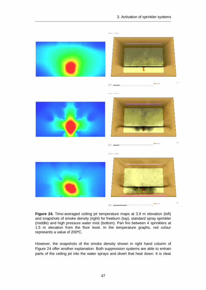
The left hand column of Figure 24 presents a gas temperature slice at 3.9 m elevation from the floor level, averaged over time in the steady-state situation (after all activations have occurred). The cooling effect of the water sprays is clearly visible in the graphs. It is also obvious that in the case of standard sprinklers, a lot of heat escapes between the first ring of sprinklers to cause activations in the second ring. Thus, one explanation for the smaller number of water mist sprinkler activations appears to be a better cooling capability.
3. Activation of sprinkler systems
47
Figure 24. Time-averaged ceiling jet temperature maps at 3.9 m elevation (left) and snapshots of smoke density (right) for freeburn (top), standard spray sprinkler (middle) and high pressure water mist (bottom). Pan fire between 4 sprinklers at 1.5 m elevation from the floor level. In the temperature graphs, red colour represents a value of 200ºC.
However, the snapshots of the smoke density shown in right hand column of Figure 24 offer another explanation. Both suppression systems are able to entrain parts of the ceiling jet into the water sprays and divert that heat down. It is clear
3. Activation of sprinkler systems
48
however that the high pressure water mist system does this more effectively. This can be attributed to the high momentum of the water sprays, and the effective momentum transfer between the high pressure water sprays and the surrounding gas. The ability of the high pressure water mist system to remove heat from the ceiling jet by a purely mechanical effect is significant. Only after the heat is captured and directed downward, will the hot gasses be cooled inside the water sprays so that the heat will not rise back to the ceiling jet to cause further activations.
3.4 FDS modelling of reduced spacing
Observing the ceiling jet temperature graphs of Figure 24, it may be argued that less high pressure water mist sprinklers activate simply because of the larger spacing. This argument is connected to the problem of reduced spacings in real installations: will a reduced spacing lead to an increased number of sprinkler activations, and should the systems therefore be hydraulically dimensioned to accommodate the absolute coverage area irrespective of the number of sprinklers inside that area?
To answer these questions, a series of FDS runs was performed for the standard sprinkler system and high pressure water mist system against the 1.7 MW pan fire scenario at 2.5 m and 4 m ceiling heights. For both systems and ceiling heights, the fires were positioned under 1 sprinkler, between 2 sprinklers, and between 4 sprinklers. The sprinklers were arranged at full spacing, 80% of the full spacing, and 60% of the full spacing. A total of 30 cases were run.
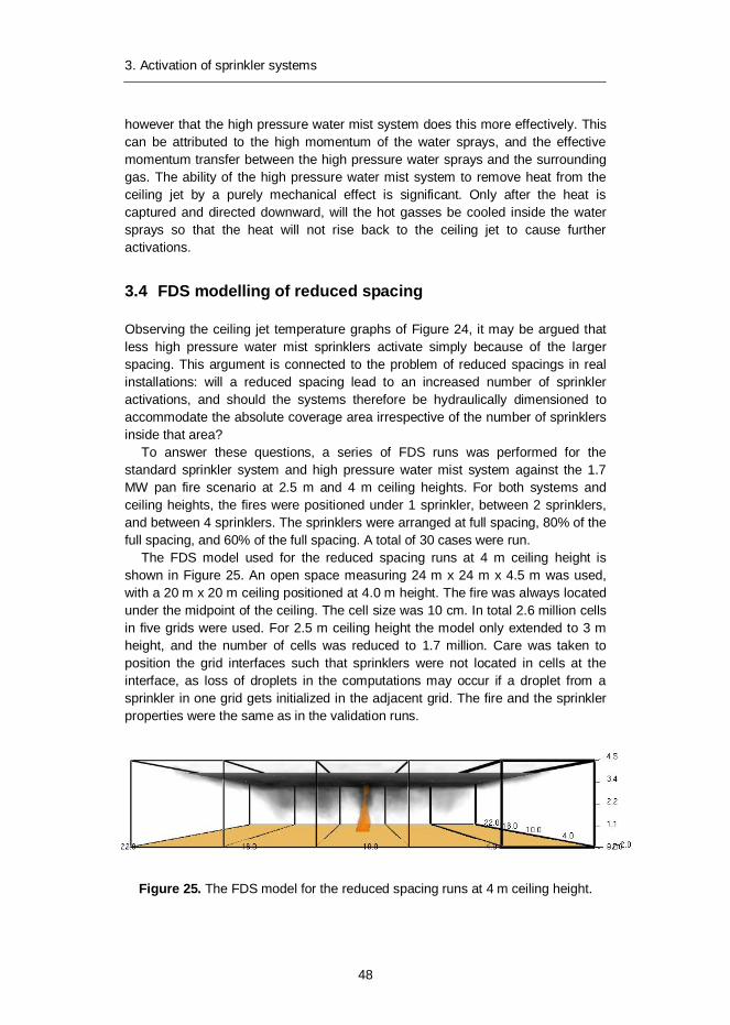
The FDS model used for the reduced spacing runs at 4 m ceiling height is shown in Figure 25. An open space measuring 24 m x 24 m x 4.5 m was used, with a 20 m x 20 m ceiling positioned at 4.0 m height. The fire was always located under the midpoint of the ceiling. The cell size was 10 cm. In total 2.6 million cells in five grids were used. For 2.5 m ceiling height the model only extended to 3 m height, and the number of cells was reduced to 1.7 million. Care was taken to position the grid interfaces such that sprinklers were not located in cells at the interface, as loss of droplets in the computations may occur if a droplet from a sprinkler in one grid gets initialized in the adjacent grid. The fire and the sprinkler properties were the same as in the validation runs.
Figure 25. The FDS model for the reduced spacing runs at 4 m ceiling height.
3. Activation of sprinkler systems
49
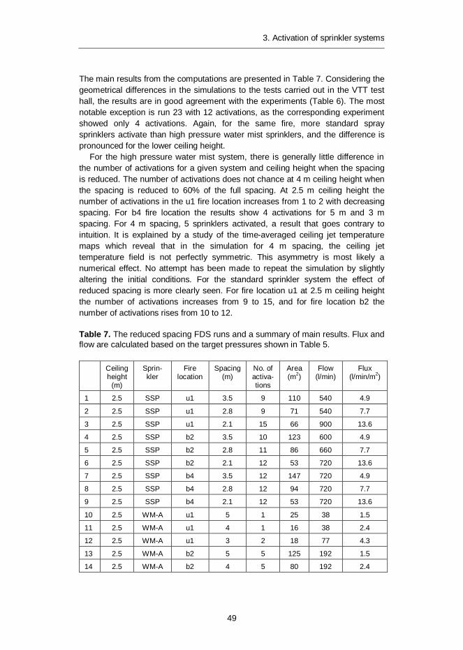
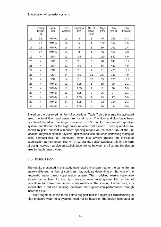
The main results from the computations are presented in Table 7. Considering the geometrical differences in the simulations to the tests carried out in the VTT test hall, the results are in good agreement with the experiments (Table 6). The most notable exception is run 23 with 12 activations, as the corresponding experiment showed only 4 activations. Again, for the same fire, more standard spray sprinklers activate than high pressure water mist sprinklers, and the difference is pronounced for the lower ceiling height.
For the high pressure water mist system, there is generally little difference in the number of activations for a given system and ceiling height when the spacing is reduced. The number of activations does not chance at 4 m ceiling height when the spacing is reduced to 60% of the full spacing. At 2.5 m ceiling height the number of activations in the u1 fire location increases from 1 to 2 with decreasing spacing. For b4 fire location the results show 4 activations for 5 m and 3 m spacing. For 4 m spacing, 5 sprinklers activated, a result that goes contrary to intuition. It is explained by a study of the time-averaged ceiling jet temperature maps which reveal that in the simulation for 4 m spacing, the ceiling jet temperature field is not perfectly symmetric. This asymmetry is most likely a numerical effect. No attempt has been made to repeat the simulation by slightly altering the initial conditions. For the standard sprinkler system the effect of reduced spacing is more clearly seen. For fire location u1 at 2.5 m ceiling height the number of activations increases from 9 to 15, and for fire location b2 the number of activations rises from 10 to 12.
Table 7. The reduced spacing FDS runs and a summary of main results. Flux and flow are calculated based on the target pressures shown in Table 5.
Ceiling height
(m)
Sprin-kler
Fire location
Spacing (m)
No. of activa-tions
Area (m2)
Flow (l/min)
Flux (l/min/m2)
1 2.5 SSP u1 3.5 9 110 540 4.9
2 2.5 SSP u1 2.8 9 71 540 7.7
3 2.5 SSP u1 2.1 15 66 900 13.6
4 2.5 SSP b2 3.5 10 123 600 4.9
5 2.5 SSP b2 2.8 11 86 660 7.7
6 2.5 SSP b2 2.1 12 53 720 13.6
7 2.5 SSP b4 3.5 12 147 720 4.9
8 2.5 SSP b4 2.8 12 94 720 7.7
9 2.5 SSP b4 2.1 12 53 720 13.6
10 2.5 WM-A u1 5 1 25 38 1.5
11 2.5 WM-A u1 4 1 16 38 2.4
12 2.5 WM-A u1 3 2 18 77 4.3
13 2.5 WM-A b2 5 5 125 192 1.5
14 2.5 WM-A b2 4 5 80 192 2.4
3. Activation of sprinkler systems
50
Ceiling height
(m)
Sprin-kler
Fire location
Spacing (m)
No. of activa-tions
Area (m2)
Flow (l/min)
Flux (l/min/m2)
15 2.5 WM-A b2 3 5 45 192 4.3
16 2.5 WM-A b4 5 4 100 154 1.5
17 2.5 WM-A b4 4 5 80 192 2.4
18 2.5 WM-A b4 3 4 36 154 4.3
19 4 SSP u1 3.5 9 110 540 4.9
20 4 SSP u1 2.1 9 40 540 13.6
21 4 SSP b2 3.5 7 86 420 4.9
22 4 SSP b2 2.1 7 31 420 13.6
23 4 SSP b4 3.5 12 147 720 4.9
24 4 SSP b4 2.1 12 53 720 13.6
25 4 WM-B u1 4.25 1 18 38 2.1
26 4 WM-B u1 2.55 1 7 38 5.9
27 4 WM-B b2 4.25 2 36 77 2.1
28 4 WM-B b2 2.55 2 13 77 5.9
29 4 WM-B b4 4.25 4 72 154 2.1
30 4 WM-B b4 2.55 4 26 154 5.9
Based on the observed number of activations, Table 7 also presents the activated area, the total flow, and water flux for all runs. The flow and flux have been calculated based on the target pressures of 0.56 bar for the standard sprinkler system, and 80 bar for the high pressure water mist system. These quantities are shown to point out that a reduced spacing means an increased flux at the fire location. In typical sprinkler system applications with fire loads consisting mainly of solid combustibles, an increased water flux always means an increased suppression performance. The NFPA 13 standard acknowledges this in the form of design curves that give an explicit dependence between the flux and the design area for each hazard class.
3.5 Discussion
The results presented in this study have explicitly shown that for the same fire, an entirely different number of sprinklers may activate depending on the type of the automatic water based suppression system. The modelling results have also shown that at least for the high pressure water mist system, the number of activations for a fixed fire depends only weakly on the spacing. Furthermore, it is known that a reduced spacing increases the suppression performance through increased flux.
Taken together, these three points suggest that the hydraulic dimensioning of high pressure water mist systems need not be based on the design rules applied

3. Activation of sprinkler systems
51
for standard sprinkler systems. Indeed, the development of hydraulic dimensioning rules for water mist systems would be technically justified. This point is elaborated in Figure 26. The protection of a known fire hazard by standard sprinkler technology involves first assigning a hazard class to the fire hazard, and then following existing design rules for the sprinkler system. This procedure is the outcome of the long tradition of sprinkler systems.
It remains to be seen whether water mist technology will evolve to a point where a simple hazard classification scheme would work together with tabulated design rules. Currently, the evolution of this technology is taking a different approach altogether, by allowing variable system designs for the same hazard, and limiting the field of applicability of a given system. At the core of this approach is the fire performance test. Each system must prove its fire suppression performance in a fire test, and the field of applicability for the system is limited by the fire tests conducted for that system. Further experience with water mist systems may yield more generic fire performance tests and wider fields of applicability.
FIRE HAZARD
Application specific Hazard classification
Fire test - design fire explicitly defined
Design rules - design fire unknown
Performance based system parameters + safety factors
Prescriptive system parameters + safety factors
Fixed number of nozzles based on the fire test
Fixed design area
Figure 26. The process of determining the hydraulic dimensioning of a suppress-ion system through a fire test (left) or based on hazard classification (right).
Fire tests are simulated fires, not real fires. They could also be called design fires, for they define the design of the suppression system. The choice of the design fire (as well as the design of the entire fire test) is obviously critically important for the
3. Activation of sprinkler systems
52
performance of the suppression system in the intended application. However, once this choice is rigorously made, it should also be trusted. Currently, however, this choice is not fully trusted. Fire testings have been conducted where the acceptance criteria have been met with a limited number of sprinkler activations, but yet in practice these systems must be designed for many more activations. These extra activations can be called safety factors.
It is not the purpose of this presentation to extensively discuss the issue of safety factors. It is pointed out however, that the safety factors should be appropriate for the system in question. Applying the safety factors of one system type to another may lead to impractical system designs. For example, the design areas of standard sprinkler systems are intended for systems that can cover an entire generic hazard class, and a large design area may be desirable in order to make sure that all possible (but unknown) fires are controlled. A large design area for a water mist system designed for a limited range of applications may represent an overdesign.
One possible way to proceed with developing water mist system design rules could be to put more trust in the fire performance test and base the hydraulic dimensioning of these systems on the number of activations observed in the fire test. This is not to say that the dimensioning area should be based exactly on the largest number of activations observed in a test. Certainly a safety factor would need to be considered, and it would probably need to depend on the intended field of applicability. But considering the results of this study, a fixed number of sprinklers instead of a fixed design area could represent a way forward.
Finally it is noted that the suggested approach also puts strict requirements for the test arrangement. In particular, the test must be able to conclusively show that a ring of non-activated sprinklers surrounds the activated sprinklers. It is clear that for applications belonging to the higher hazard classes, the physical dimension of the test can increase significantly.
4. Cooling performance
53
4. Cooling performance
Water is the oldest known fire suppression agent, and today, despite the recent developments in the field of physical and chemical suppression agents, it still remains the agent of choice for numerous applications. On a mass basis, finely divided water mist can at least as effective as Halon 1301 (CF3Br) (Zegers et al. 2000) a fact that has prompted a lot of detailed studies on the suppression effectiveness and suppression mechanisms of water. These studies have shown that the suppression effect of liquid water as well as water vapour is for all practical purposes physical, and can be attributed to the large latent heat of evaporation of water, and the heat capacity of water vapour. Cooling of the flame and cooling of the fuel surfaces are two primary extinguishing mechanisms of water. In addition, the attenuation of thermal radiation is considered an important secondary extinguishing mechanism especially for water mist.
4.1 Cooling of fire plumes
Despite the fire itself, the cooling capability of water may also affect the surroundings of a fire, particularly the load-bearing capability of structures. For example, fires in high-rise storage areas can lead to extreme heat loads to the ceiling structures unless a sprinkler system is installed to control or to suppress the fire and to provide cooling to structures. Thus, the NFPA 13 sprinkler rules state that building steel structures (in storage areas) do not require special (passive) protection measures provided that the sprinkler system is installed to the appropriate protection requirements. On the contrary, the European sprinkler rules (EN12845 or CEA4001) do not explicitly mention steel structures, an issue that may cause confusion and even lead to excessive protection requirements in practice. To gain insight into the cooling effectiveness of a sprinkler system, this chapter presents simulations on temperatures of a fire plume with and without a sprinkler system. It should be stressed that these simulations purposefully neglect the solid fire loads present in practical applications in order to focus entirely on the cooling performance.
4. Cooling performance
54
4.1.1 Sprinkler modelling
The cooling simulations were performed for two types of sprinklers: standard spray sprinklers (SSP) and early suppression fast response (ESFR) sprinklers. Both sprinkler types have the same basic design. Water jet emerging from the circular discharge orifice impacts on a deflector plate that redirects the flow and forms the water into a spray. Deflector plates come in a variety of designs. Generally, plates designed for standard spray sprinklers result in a parabolic spray envelope that is directed downwards such that no water is directly hitting the ceiling above the sprinkler. However, little or no water is discharged directly below the deflector plate. Detailed analyses of sprinkler discharge patterns (Sheppard 2002) indicate that on the average sprinklers having a discharge orifice diameter less than 25 mm discharge most of the water around elevation angle of 60 degrees from vertical. However due to aerodynamic effects the water distribution at floor level is more uniform as especially the finer droplets tend to accumulate towards the centre of the spray.
The ESFR deflector plate design differs from SSP such that it allows more water to be discharged directly below the sprinkler. The ESFR sprinkler is specifically designed for high-pile storage applications where sprinklers installed directly in storage racks are not desired or possible. A storage fire may result in a fast-growing fire where vertical flow velocities in the fire plume are high. The purpose of the central core discharge in the spray pattern is to effectively counter the buoyant flow and to suppress the fire at an early stage of growth.
The water jet exit velocity from the discharge orifice is obtained from Bernoulli’s law as
(19)
where p is the pressure of the fluid in the orifice, and is the density of the fluid. However due to the interaction of the water jet with the deflector plate, and the atomization process, the droplet initial velocities some 10 cm away from the deflector plate are generally about 60% of the jet exit velocity.
The droplet size spectrum due to atomization is often described by a mathematical function such as a log-normal or a Rosin-Rammler distribution. There is no fundamental reason why the droplet size spectrum should conform with any standard distribution, these are used for convenience. FDS assumes, based on Sheppard (2002), a combination of log-normal (for fine droplets below median volume diameter) and Rosin-Rammler (for coarse droplets above median volume diameter) distributions. This is convenient as the user needs only to provide the median volume diameter and optionally another parameter defining the width of the distribution. However there is often little or no information available
pv 2
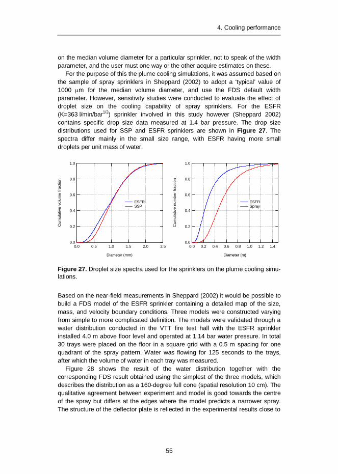
4. Cooling performance
55
on the median volume diameter for a particular sprinkler, not to speak of the width parameter, and the user must one way or the other acquire estimates on these.
For the purpose of this the plume cooling simulations, it was assumed based on the sample of spray sprinklers in Sheppard (2002) to adopt a ‘typical’ value of 1000 m for the median volume diameter, and use the FDS default width parameter. However, sensitivity studies were conducted to evaluate the effect of droplet size on the cooling capability of spray sprinklers. For the ESFR (K=363 l/min/bar1/2) sprinkler involved in this study however (Sheppard 2002) contains specific drop size data measured at 1.4 bar pressure. The drop size distributions used for SSP and ESFR sprinklers are shown in Figure 27. The spectra differ mainly in the small size range, with ESFR having more small droplets per unit mass of water.
Figure 27. Droplet size spectra used for the sprinklers on the plume cooling simu-lations.
Based on the near-field measurements in Sheppard (2002) it would be possible to build a FDS model of the ESFR sprinkler containing a detailed map of the size, mass, and velocity boundary conditions. Three models were constructed varying from simple to more complicated definition. The models were validated through a water distribution conducted in the VTT fire test hall with the ESFR sprinkler installed 4.0 m above floor level and operated at 1.14 bar water pressure. In total 30 trays were placed on the floor in a square grid with a 0.5 m spacing for one quadrant of the spray pattern. Water was flowing for 125 seconds to the trays, after which the volume of water in each tray was measured.
Figure 28 shows the result of the water distribution together with the corresponding FDS result obtained using the simplest of the three models, which describes the distribution as a 160-degree full cone (spatial resolution 10 cm). The qualitative agreement between experiment and model is good towards the centre of the spray but differs at the edges where the model predicts a narrower spray. The structure of the deflector plate is reflected in the experimental results close to
1.0
0.8
0.6
0.4
0.2
0.0
Cum
ulat
ive
volu
me
fract
ion
2.52.01.51.00.50.0
Diameter (mm)
ESFR SSP
1.0
0.8
0.6
0.4
0.2
0.0
Cum
ulat
ive
num
ber f
ract
ion
1.41.21.00.80.60.40.20.0
Diameter (m)
ESFR Spray

4. Cooling performance
56
the edge. For the FDS model however the reason for the azimuthal structure must be numerical since the boundary condition for the droplets is entirely symmetric around the vertical axis. It turned out that adding complexity to the nozzle definition made the agreement worse (the modelled spray became even narrower) and therefore the simple description was used for the plume cooling simulations.
Figure 28. Experimental (left) and simulated (right) water distribution of an ESFR sprinkler (K-factor 363 l/min/bar1/2, pressure 1.14 bar, height 4 m). The contour class units are grams of water.
In storage applications, both SSP and ESFR sprinklers are normally installed with a protected area of 9 m2 per sprinkler (3 m spacing) (EN 12845). This was also the sprinkler spacing used in the modelling.
4.1.2 Plume cooling model
The FDS model of the plume cooling simulation is shown in Figure 29. The computational domain is a cube with a side of 10 m. The spatial resolution is 10 cm. The plume is generated by a propane burner measuring 3.2 m x 3.2 m. Heat release rates of 5 MW, 10 MW, 15 MW and 20 MW were considered. Four sprinklers were installed 0.3 m below the ceiling such that the plume axis was between the four sprinklers. Point devices were placed along the plume axis to measure gas temperatures. The simulation also included a steel beam system above the plume as well as an insulated steel sheet ceiling, both of which were instrumented for surface temperatures. The simulations were run for at least 200 seconds. The first 60 seconds were run without the water sprays to establish the plume. Time-averaged gas temperatures in the freely burning and cooled plumes were computed from the point device outputs.
0 0.5 1 1.5 2 2.5 3 3.5 40
0.5
1
1.5
2
2.5
3
3.5
4
5500-6000
5000-5500
4500-5000
4000-4500
3500-4000
3000-3500
2500-3000
2000-2500
1500-2000
1000-1500
500-1000
0-500
0 0.5 1 1.5 2 2.5 3 3.5 40
0.5
1
1.5
2
2.5
3
3.5
4
5500-60005000-55004500-50004000-45003500-40003000-35002500-30002000-25001500-20001000-1500500-10000-500
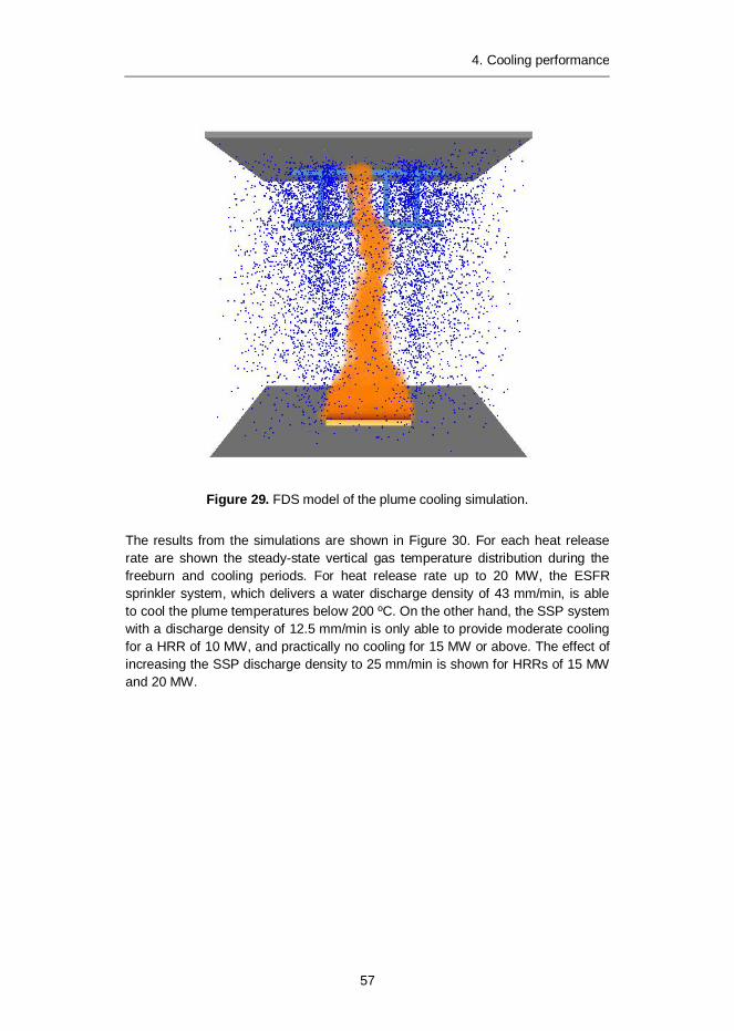
4. Cooling performance
57
Figure 29. FDS model of the plume cooling simulation.
The results from the simulations are shown in Figure 30. For each heat release rate are shown the steady-state vertical gas temperature distribution during the freeburn and cooling periods. For heat release rate up to 20 MW, the ESFR sprinkler system, which delivers a water discharge density of 43 mm/min, is able to cool the plume temperatures below 200 ºC. On the other hand, the SSP system with a discharge density of 12.5 mm/min is only able to provide moderate cooling for a HRR of 10 MW, and practically no cooling for 15 MW or above. The effect of increasing the SSP discharge density to 25 mm/min is shown for HRRs of 15 MW and 20 MW.
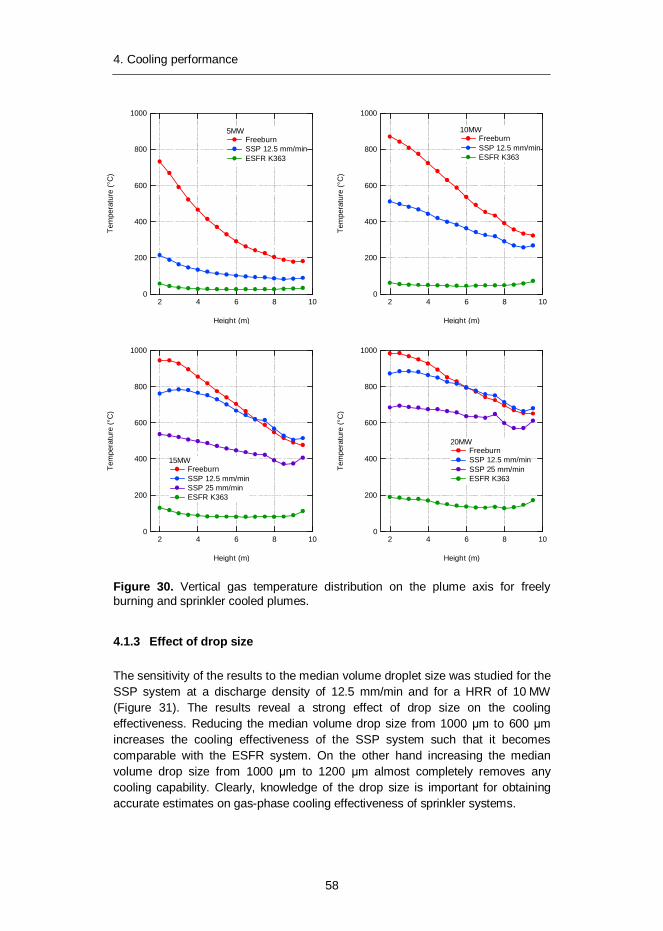
4. Cooling performance
58
Figure 30. Vertical gas temperature distribution on the plume axis for freely burning and sprinkler cooled plumes.
4.1.3 Effect of drop size
The sensitivity of the results to the median volume droplet size was studied for the SSP system at a discharge density of 12.5 mm/min and for a HRR of 10 MW (Figure 31). The results reveal a strong effect of drop size on the cooling effectiveness. Reducing the median volume drop size from 1000 m to 600 m increases the cooling effectiveness of the SSP system such that it becomes comparable with the ESFR system. On the other hand increasing the median volume drop size from 1000 m to 1200 m almost completely removes any cooling capability. Clearly, knowledge of the drop size is important for obtaining accurate estimates on gas-phase cooling effectiveness of sprinkler systems.
1000
800
600
400
200
0
Tem
pera
ture
(°C
)
108642
Height (m)
5MW Freeburn SSP 12.5 mm/min ESFR K363
1000
800
600
400
200
0
Tem
pera
ture
(°C
)
108642
Height (m)
10MW Freeburn SSP 12.5 mm/min ESFR K363
1000
800
600
400
200
0
Tem
pera
ture
(°C
)
108642
Height (m)
15MW Freeburn SSP 12.5 mm/min SSP 25 mm/min ESFR K363
1000
800
600
400
200
0
Tem
pera
ture
(°C
)
108642
Height (m)
20MW Freeburn SSP 12.5 mm/min SSP 25 mm/min ESFR K363
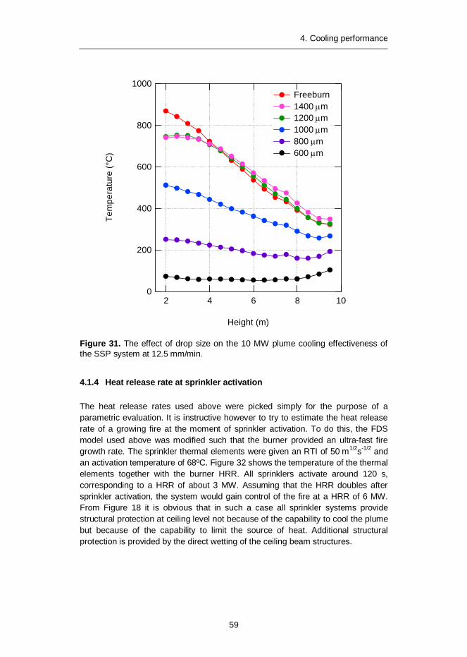
4. Cooling performance
59
Figure 31. The effect of drop size on the 10 MW plume cooling effectiveness of the SSP system at 12.5 mm/min.
4.1.4 Heat release rate at sprinkler activation
The heat release rates used above were picked simply for the purpose of a parametric evaluation. It is instructive however to try to estimate the heat release rate of a growing fire at the moment of sprinkler activation. To do this, the FDS model used above was modified such that the burner provided an ultra-fast fire growth rate. The sprinkler thermal elements were given an RTI of 50 m1/2s-1/2 and an activation temperature of 68ºC. Figure 32 shows the temperature of the thermal elements together with the burner HRR. All sprinklers activate around 120 s, corresponding to a HRR of about 3 MW. Assuming that the HRR doubles after sprinkler activation, the system would gain control of the fire at a HRR of 6 MW. From Figure 18 it is obvious that in such a case all sprinkler systems provide structural protection at ceiling level not because of the capability to cool the plume but because of the capability to limit the source of heat. Additional structural protection is provided by the direct wetting of the ceiling beam structures.
1000
800
600
400
200
0
Tem
pera
ture
(°C
)
108642
Height (m)
Freeburn 1400 m 1200 m 1000 m 800 m 600 m
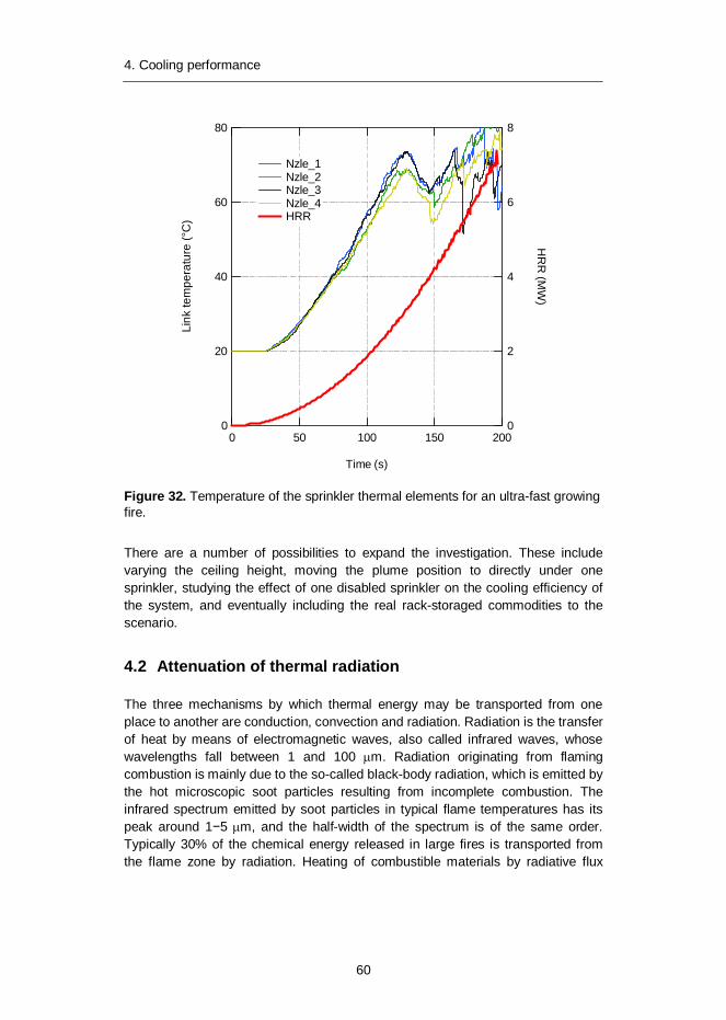
4. Cooling performance
60
Figure 32. Temperature of the sprinkler thermal elements for an ultra-fast growing fire.
There are a number of possibilities to expand the investigation. These include varying the ceiling height, moving the plume position to directly under one sprinkler, studying the effect of one disabled sprinkler on the cooling efficiency of the system, and eventually including the real rack-storaged commodities to the scenario.
4.2 Attenuation of thermal radiation
The three mechanisms by which thermal energy may be transported from one place to another are conduction, convection and radiation. Radiation is the transfer of heat by means of electromagnetic waves, also called infrared waves, whose wavelengths fall between 1 and 100 m. Radiation originating from flaming combustion is mainly due to the so-called black-body radiation, which is emitted by the hot microscopic soot particles resulting from incomplete combustion. The infrared spectrum emitted by soot particles in typical flame temperatures has its peak around 1 5 m, and the half-width of the spectrum is of the same order. Typically 30% of the chemical energy released in large fires is transported from the flame zone by radiation. Heating of combustible materials by radiative flux
80
60
40
20
0
Link
tem
pera
ture
(°C
)
200150100500
Time (s)
8
6
4
2
0
HR
R (M
W)
Nzle_1 Nzle_2 Nzle_3 Nzle_4 HRR

4. Cooling performance
61
from the flames is an important fire spread mechanism. High radiative flux levels may also prevent manual fire fighting operations.
This chapter presents first an experimental investigation on the capability of water mist sprays to attenuate radiation, followed by simulations of the experi-ments in order to evaluate the current capability of FDS to treat attenuation or radiation by small particles.
4.2.1 Experimental set-up
The general idea in the experiments was to measure the total radiative flux from a heat source with and without a water spray between the heat source and a heat flux gauge. Ideally, the heat source should provide black-body radiation, whose intensity is sufficiently high considering the measurement range of the heat flux gauge, and does not fluctuate or drift as a function of time. In addition, the water spray between the heat source and the gauge should wet neither the heat source nor the gauge. In practice, the available hardware will limit the design of the set-up.
The experiments were carried out in the VTT large fire test hall. A schematic diagram of the experimental arrangement is shown in Figure 33 and a photograph of the set-up is shown in Figure 34. The heat source was a LPG gas heater unit with a total heat output of 3.25 kW. The radiative panel of the unit measured about 20 cm x 30 cm. The maximum surface temperature of the panel was 950 C, as measured by a hand-held K-type thermocouple probe. The panel was oriented in a vertical plane such that the convective heat flow from the panel would not reach the heat flux gauge and would not interfere with the water spray.

4. Cooling performance
62
Figure 33. Schematic diagram of the experimental arrangement for radiation attenuation tests.
Figure 34. Experimental set-up for measuring the radiation attenuation by water mist micro nozzles.
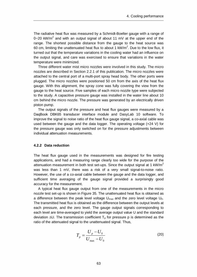
4. Cooling performance
63
The radiative heat flux was measured by a Schmidt-Boelter gauge with a range of 20 kW/m2 and with an output signal of about 11 mV at the upper end of the
range. The shortest possible distance from the gauge to the heat source was 60 cm, limiting the unattenuated heat flux to about 1 kW/m2. Due to the low flux, it turned out that the temperature variations in the cooling water had an influence on the output signal, and care was exercised to ensure that variations in the water temperature were minimized.
Three different water mist micro nozzles were involved in this study. The micro nozzles are described in Section 2.2.1 of this publication. The micro nozzles were attached to the central port of a multi-port spray head body. The other ports were plugged. The micro nozzles were positioned 50 cm from the axis of the heat flux gauge. With this alignment, the spray cone was fully covering the view from the gauge to the heat source. Five samples of each micro nozzle type were subjected to the study. A capacitive pressure gauge was installed in the water line about 10 cm behind the micro nozzle. The pressure was generated by an electrically driven piston pump.
The output signals of the pressure and heat flux gauges were measured by a DaqBook DBK65 transducer interface module and DasyLab 10 software. To improve the signal to noise ratio of the heat flux gauge signal, a co-axial cable was used between the gauge and the data logger. The operating voltage (+24 V) for the pressure gauge was only switched on for the pressure adjustments between individual attenuation measurements.
4.2.2 Data reduction
The heat flux gauge used in the measurements was designed for fire testing applications, and had a measuring range clearly too wide for the purpose of the attenuation measurement in both test set-ups. Since the output signal at 1 kW/m2 was less than 1 mV, there was a risk of a very small signal-to-noise ratio. However, the use of a co-axial cable between the gauge and the data logger, and sufficient time averaging of the gauge signal provided a surprisingly good accuracy for the measurement.
A typical heat flux gauge output from one of the measurements in the micro nozzle test set-up is shown in Figure 35. The unattenuated heat flux is obtained as a difference between the peak level voltage Umax and the zero level voltage U0. The transmitted heat flux is obtained as the difference between the output levels at each pressure, and the zero level. The gauge output signals corresponding to each level are time-averaged to yield the average output value U and the standard deviation U. The transmission coefficient Tp for pressure p is determined as the ratio of the attenuated signal to the unattenuated signal. Thus,
0max
0
UUUU
T pp (20)

4. Cooling performance
64
because the heat flux incident on the gauge is linearly proportional to the output voltage. In case of micro nozzles, five samples of each micro nozzle types were used in the experiments. The quantities U0, Umax and Up and their error estimates can be obtained as the weighted means and their standard deviations over five individual determinations. As an example, for Up we have
5
1
2,
5
1
2,,
1i
ip
iipip
p
U
UUU (21)
and
5
1
2,1
1
iip
p
UU
(22)
The absolute error for the transmission coefficient is given by the partial derivatives as
020max
0
0max
max20max
0
0max
1
1
UUUUU
UU
UUUUU
UUU
T
p
ppp
(23)
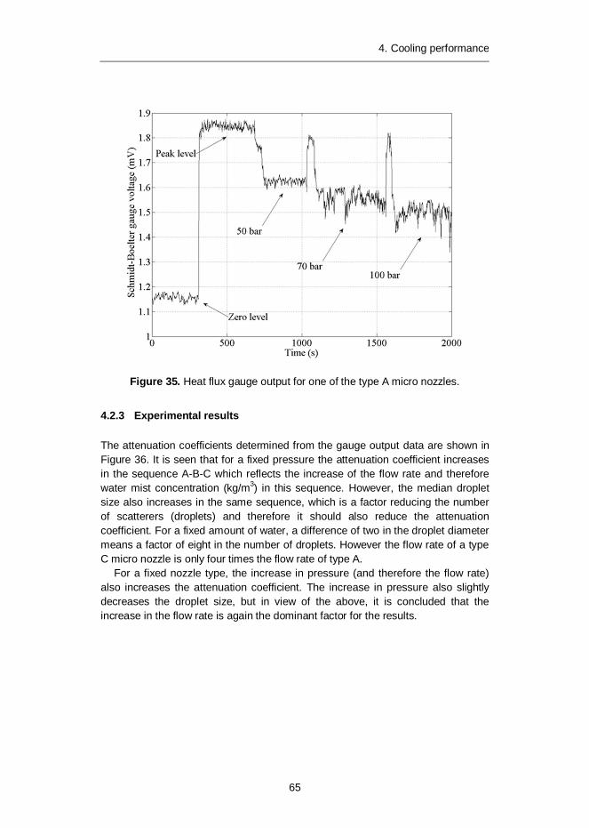
4. Cooling performance
65
Figure 35. Heat flux gauge output for one of the type A micro nozzles.
4.2.3 Experimental results
The attenuation coefficients determined from the gauge output data are shown in Figure 36. It is seen that for a fixed pressure the attenuation coefficient increases in the sequence A-B-C which reflects the increase of the flow rate and therefore water mist concentration (kg/m3) in this sequence. However, the median droplet size also increases in the same sequence, which is a factor reducing the number of scatterers (droplets) and therefore it should also reduce the attenuation coefficient. For a fixed amount of water, a difference of two in the droplet diameter means a factor of eight in the number of droplets. However the flow rate of a type C micro nozzle is only four times the flow rate of type A.
For a fixed nozzle type, the increase in pressure (and therefore the flow rate) also increases the attenuation coefficient. The increase in pressure also slightly decreases the droplet size, but in view of the above, it is concluded that the increase in the flow rate is again the dominant factor for the results.
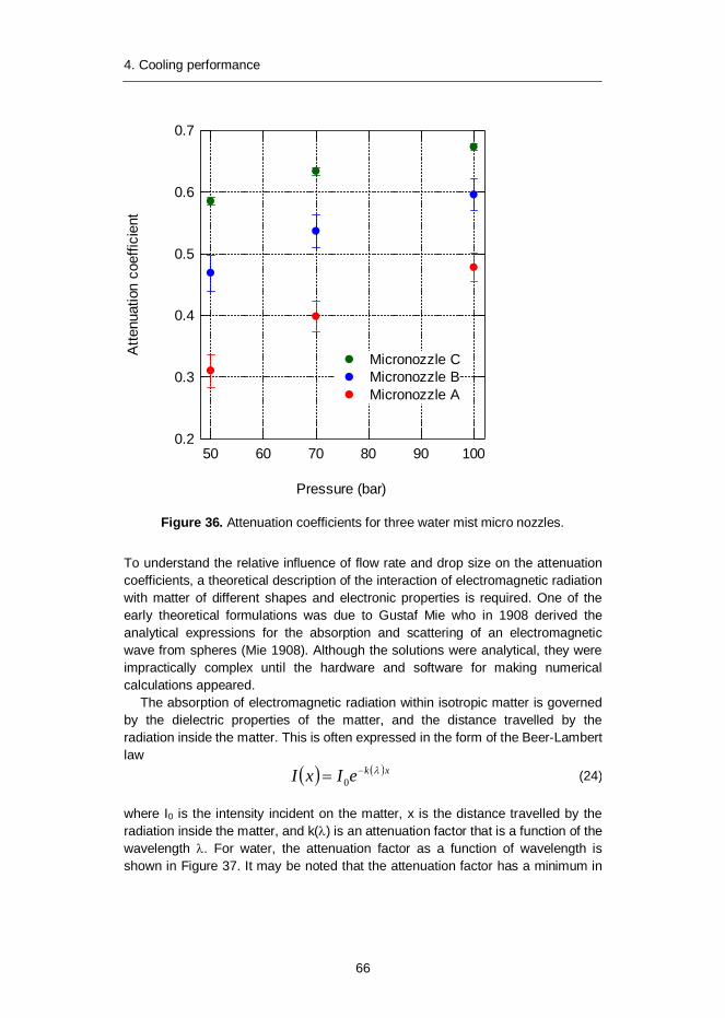
4. Cooling performance
66
Figure 36. Attenuation coefficients for three water mist micro nozzles.
To understand the relative influence of flow rate and drop size on the attenuation coefficients, a theoretical description of the interaction of electromagnetic radiation with matter of different shapes and electronic properties is required. One of the early theoretical formulations was due to Gustaf Mie who in 1908 derived the analytical expressions for the absorption and scattering of an electromagnetic wave from spheres (Mie 1908). Although the solutions were analytical, they were impractically complex until the hardware and software for making numerical calculations appeared.
The absorption of electromagnetic radiation within isotropic matter is governed by the dielectric properties of the matter, and the distance travelled by the radiation inside the matter. This is often expressed in the form of the Beer-Lambert law
xkeIxI 0 (24)
where I0 is the intensity incident on the matter, x is the distance travelled by the radiation inside the matter, and k( ) is an attenuation factor that is a function of the wavelength . For water, the attenuation factor as a function of wavelength is shown in Figure 37. It may be noted that the attenuation factor has a minimum in
0.7
0.6
0.5
0.4
0.3
0.2
Atte
nuat
ion
coef
ficie
nt
1009080706050
Pressure (bar)
Micronozzle C Micronozzle B Micronozzle A

4. Cooling performance
67
the visible wavelength range around turquoise colour (475 nm), and a maximum around 2.9 m.
Figure 37. The attenuation factor for electromagnetic radiation in liquid water (Hale & Quarry 1973).
The physical parameters governing the scattering process are the index of refraction, the scattering angle, and, importantly, the ratio of the sphere diameter to the wavelength, as defined in the form (Özisik 1973)
Dx (25)
The significance of x lies in the fact that the scattering cross section has its maximum for values of x close to 1. In other words, the scattering efficiency is at maximum when the wavelength of the wave and the diameter of the scatterer are equal. Given the fact that the black-body radiation spectrum emitted by a flame peaks around 2 m, it is evident that the smallest droplets produced by the present water mist systems are the most effective contributors to scattering of heat radiation.
10-1
100
101
102
103
104
105
106
Atte
nuat
ion
fact
or (1
/m)
2 4 6 8
10-62 4 6 8
10-52 4 6 8
10-42
Wavelength ( m)

4. Cooling performance
68
The attenuation of thermal radiation from a black-body heat source by water mist sprays involves a spectrum of wavelengths and drop sizes. The attenuation coefficients determined in this study represent integral values over both spectrums. The integrated cross sections for absorption and scattering processes can be computed for example using relevant parts of the code contained in FDS. The integrated absorption and scattering cross sections as a function of median volume drop size (for the default FDS drop size distribution) are shown in Figure 38, together with the cumulative number fraction (CNF) spectrum measured for type A micro nozzle. The discretization interval for the drop size in the measurements was 10 m. The digital imaging technique was not capable of detecting any droplets in the smallest size bin of 0 10 m. Nevertheless, it is obvious from the CNF curve that the majority of the water volume for type A nozzle (at 70 bar) is in droplets of such size that the absorption process has a larger cross section than the scattering process. Since type B and type C nozzles produce (on the average) larger droplets, Figure 38 effectively explains why the flow rate, and therefore the water volumetric concentration, is the dominant factor in determining the attenuation coefficient for thermal radiation.
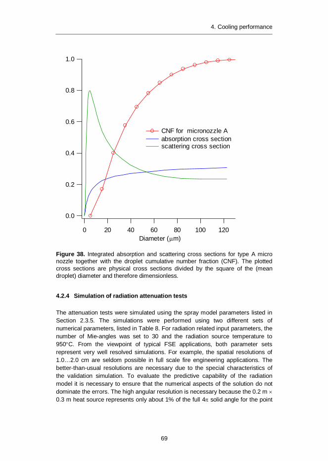
4. Cooling performance
69
Figure 38. Integrated absorption and scattering cross sections for type A micro nozzle together with the droplet cumulative number fraction (CNF). The plotted cross sections are physical cross sections divided by the square of the (mean droplet) diameter and therefore dimensionless.
4.2.4 Simulation of radiation attenuation tests
The attenuation tests were simulated using the spray model parameters listed in Section 2.3.5. The simulations were performed using two different sets of numerical parameters, listed in Table 8. For radiation related input parameters, the number of Mie-angles was set to 30 and the radiation source temperature to 950 C. From the viewpoint of typical FSE applications, both parameter sets represent very well resolved simulations. For example, the spatial resolutions of 1.0…2.0 cm are seldom possible in full scale fire engineering applications. The better-than-usual resolutions are necessary due to the special characteristics of the validation simulation. To evaluate the predictive capability of the radiation model it is necessary to ensure that the numerical aspects of the solution do not dominate the errors. The high angular resolution is necessary because the 0.2 m 0.3 m heat source represents only about 1% of the full 4 solid angle for the point
1.0
0.8
0.6
0.4
0.2
0.0
120100806040200Diameter ( m)
CNF for micronozzle A absorption cross section scattering cross section
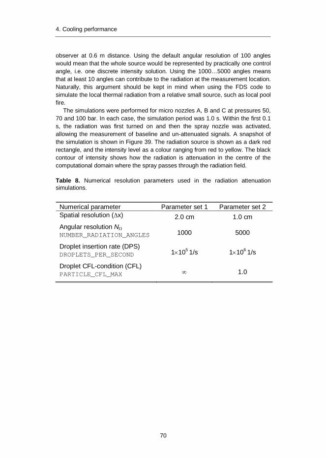
4. Cooling performance
70
observer at 0.6 m distance. Using the default angular resolution of 100 angles would mean that the whole source would be represented by practically one control angle, i.e. one discrete intensity solution. Using the 1000…5000 angles means that at least 10 angles can contribute to the radiation at the measurement location. Naturally, this argument should be kept in mind when using the FDS code to simulate the local thermal radiation from a relative small source, such as local pool fire.
The simulations were performed for micro nozzles A, B and C at pressures 50, 70 and 100 bar. In each case, the simulation period was 1.0 s. Within the first 0.1 s, the radiation was first turned on and then the spray nozzle was activated, allowing the measurement of baseline and un-attenuated signals. A snapshot of the simulation is shown in Figure 39. The radiation source is shown as a dark red rectangle, and the intensity level as a colour ranging from red to yellow. The black contour of intensity shows how the radiation is attenuation in the centre of the computational domain where the spray passes through the radiation field.
Table 8. Numerical resolution parameters used in the radiation attenuation simulations.
Numerical parameter Parameter set 1 Parameter set 2 Spatial resolution ( x) 2.0 cm 1.0 cm Angular resolution N NUMBER_RADIATION_ANGLES 1000 5000
Droplet insertion rate (DPS) DROPLETS_PER_SECOND 1 105 1/s 1 106 1/s
Droplet CFL-condition (CFL) PARTICLE_CFL_MAX 1.0
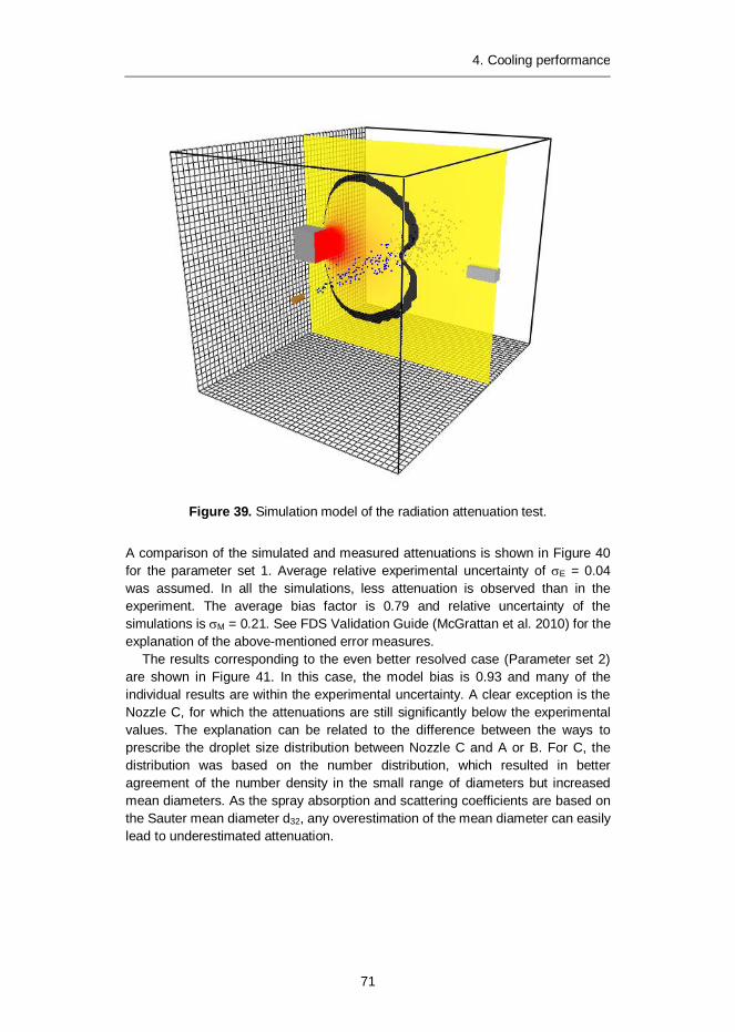
4. Cooling performance
71
Figure 39. Simulation model of the radiation attenuation test.
A comparison of the simulated and measured attenuations is shown in Figure 40 for the parameter set 1. Average relative experimental uncertainty of E = 0.04 was assumed. In all the simulations, less attenuation is observed than in the experiment. The average bias factor is 0.79 and relative uncertainty of the simulations is M = 0.21. See FDS Validation Guide (McGrattan et al. 2010) for the explanation of the above-mentioned error measures.
The results corresponding to the even better resolved case (Parameter set 2) are shown in Figure 41. In this case, the model bias is 0.93 and many of the individual results are within the experimental uncertainty. A clear exception is the Nozzle C, for which the attenuations are still significantly below the experimental values. The explanation can be related to the difference between the ways to prescribe the droplet size distribution between Nozzle C and A or B. For C, the distribution was based on the number distribution, which resulted in better agreement of the number density in the small range of diameters but increased mean diameters. As the spray absorption and scattering coefficients are based on the Sauter mean diameter d32, any overestimation of the mean diameter can easily lead to underestimated attenuation.
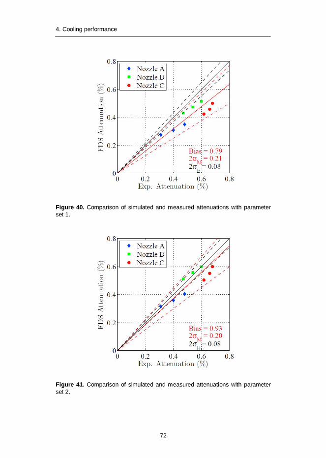
4. Cooling performance
72
Figure 40. Comparison of simulated and measured attenuations with parameter set 1.
Figure 41. Comparison of simulated and measured attenuations with parameter set 2.
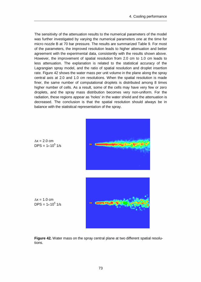
4. Cooling performance
73
The sensitivity of the attenuation results to the numerical parameters of the model was further investigated by varying the numerical parameters one at the time for micro nozzle B at 70 bar pressure. The results are summarized Table 9. For most of the parameters, the improved resolution leads to higher attenuation and better agreement with the experimental data, consistently with the results shown above. However, the improvement of spatial resolution from 2.0 cm to 1.0 cm leads to less attenuation. The explanation is related to the statistical accuracy of the Lagrangian spray model, and the ratio of spatial resolution and droplet insertion rate. Figure 42 shows the water mass per unit volume in the plane along the spray central axis at 2.0 and 1.0 cm resolutions. When the spatial resolution is made finer, the same number of computational droplets is distributed among 8 times higher number of cells. As a result, some of the cells may have very few or zero droplets, and the spray mass distribution becomes very non-uniform. For the radiation, these regions appear as ‘holes’ in the water shield and the attenuation is decreased. The conclusion is that the spatial resolution should always be in balance with the statistical representation of the spray.
x = 2.0 cm DPS = 1 105 1/s
x = 1.0 cm DPS = 1 105 1/s
Figure 42. Water mass on the spray central plane at two different spatial resolu-tions.
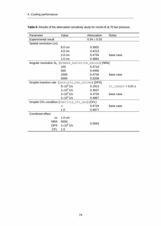
4. Cooling performance
74
Table 9. Results of the attenuation sensitivity study for nozzle B at 70 bar pressure.
Parameter Value Attenuation Notes Experimental result 0.54 0.03 Spatial resolution ( x) 8.0 cm 0.3502 4.0 cm 0.4213 2.0 cm 0.4734 base case 1.0 cm 0.3882 Angular resolution N (NUMBER_RADIATION_ANGLES) (NRA) 100 0.3710 500 0.4456 1000 0.4734 base case 5000 0.5208 Droplet insertion rate (DROPLETS_PER_SECOND) (DPS) 5 103
1/s 0.1913 DT_INSERT = 0.01 s 1 104 1/s 0.3637 1 105 1/s 0.4734 base case 1 106 1/s 0.4867 Droplet CFL-condition (PARTICLE_CFL_MAX) (CFL) 0.4734 base case 1.0 0.4877 Combined effect
x 1.0 cm
0.5563
NRA 5000 DPS 1 106 1/s CFL 1.0

5. Flame suppression
75
5. Flame suppression
Fire simulation tools based on computational fluid dynamics (CFD) are increasingly used in performance-based fire safety engineering. The tools are particularly suitable for predicting the spread of heat and smoke in complex enclosures, and generally predicting the ‘far-field’ conditions, i.e. conditions far from the flame region. Large-scale CFD simulations are typically conducted at a spatial resolution of 0.1 m or above. Such resolution is clearly too coarse compared to the resolution needed to resolve the physical and chemical processes near or in the flame, which occur on a length scale of 0.001 m or less. For these cases, FDS uses a combustion model based on the mixture fraction concept.
Generally a ‘mixture fraction’ can be defined as the ratio of the mass of a certain set of gas species to the mass of all gas species in a given volume. For combustion applications, the mixture fraction is defined as the mass fraction of the gas mixture that originates in the fuel stream. FDS versions 2 through 4 used a single parameter mixture fraction to track fuel and combustion product species. Essentially this was a ‘mixed is burned’ model: it was assumed that whenever fuel and oxygen is found in the same cell, these react immediately and completely. Among the issues of that approach was that it was unable to simulate extinction; heat release could be disabled but product formation could not.
5.1 Combustion model in FDS v.5
The release of FDS version 5 brought with it a new species tracking approach using a lumped species approach to conserve computational resources. FDS 5 by default uses a two-parameter mixture fraction that is capable of explicitly tracking unburned fuel and burned fuel (e.g. a lumped species consisting of all combustion products) and implicitly tracking the lumped species of air (e.g. everything that is not fuel or burned fuel) (Floyd & McGrattan 2009). Since combustion products are transported as a distinct species, true extinction can be modelled in FDS 5 (no heat release and no product formation). Naturally, this is an important pre-requisite for modelling under ventilated fires or fires that are suppressed by an inert gas agent.
5. Flame suppression
76
In some cases it may be desirable to predict the formation of carbon monoxide resulting from incomplete combustion. For these purposes, FDS 5 includes the possibility to further decompose the mixture fraction into three components. Choosing this option also chooses the combustion chemistry. Whereas the two-parameter mixture fraction assumes direct oxidation of fuel into CO2, the three-parameter mixture fraction invokes a two-step treatment of combustion. In this approach, all fuel that undergoes combustion is oxidized to CO in the first step. In the second step, CO is further oxidized to CO2. It is assumed that the latter step occurs always in those cells where a flame is present (to the extent that CO and O2 is available), but elsewhere the CO conversion rate is dependent on the local temperature in the Arrhenius formulation.
5.1.1 Flame extinguishing criterion
Regardless of the number of mixture fraction parameters, FDS 5 uses the following relationship between the oxygen mass fraction within the control volume and the adiabatic temperature rise of the control volume to determine whether combustion is possible
(26)
where Tm is the temperature of the control volume. By assuming an average specific heat of 1.2 kJ/(kg K) and a critical flame temperature of 1700 K, one gets the following approximate expression for the limiting oxygen mass fraction as a function of temperature:
(27)
At 293 K (20 C), the limiting oxygen concentration is 0.129, and falls linearly to zero at 1700 K (1427 C).
In the numerical implementation of this criterion, each cell is investigated for the extinguishing criterion before the actual combustion reactions are computed, provided the logical parameter SUPPRESSION has the value .TRUE.. However, when deciding whether combustion can occur in the current cell, not only the cell itself but in addition the immediate six nearest neighbours are checked. If the limiting oxygen concentration is exceeded in any of these seven cells, combustion can occur in the current cell. The extinguishment model is controlled by the following three parameters on the REAC line:
CRITICAL_FLAME_TEMPERATURE (default 1427 C) X_O2_LL (default 0.15 mol/mol) Y_F_LFL (default 0 kg/kg)
2
lim,2
O
mfpO rH
TTcY
KTTY mm
O5
lim,2 1016.91557.01310017002.1
5. Flame suppression
77
It should be noted that setting a non-zero value for Y_F_LFL means that fires in the simulations do not ignite spontaneously, and a means of igniting the fuel vapours needs to be included in the simulation.
5.1.2 Analysis of the flame extinguishing criterion
The flame extinguishing effectiveness of inert gas fire extinguishing agents can be fairly accurately attributed to the heat capacity of the agents and the existence of a critical flame temperature below which combustion reactions cannot propagate (Senecal 2005). For a given fuel, the volumetric extinguishing concentration of the agent increases with decreasing specific heat of the agent. Thus, for common inert gas agents, the flame extinguishing effectiveness can be ranked as follows:
Ar < N2 < CO2
It can be noted that Ar is a monatomic agent, nitrogen is a diatomic agent, and carbon dioxide is a triatomic agent. In general, the increased structural complexity of a molecule increases the possibilities to store thermal energy in rotational and vibrational modes. The mass of the molecule plays a secondary role to the structural complexity. For example, the room temperature specific heat of CO2 (37.1 J/(mol K)) is close to that of gaseous H2O (33.6 J/(mol K)) even though there is a significant difference in the molecular mass.
Figure 43 shows the specific heat of common inert gases and ethylene (as an example of a hydrocarbon fuel) as a function of temperature. It can be observed that the average specific heat of 1.2 kJ/(kg K) is a fair approximation for oxygen and nitrogen (i.e. normal air) as well as carbon dioxide between room and flame temperatures. However, it significantly deviates from the numbers appropriate for monatomic inert gas agents (He, Ar) and an important inert gas agent, water vapour.
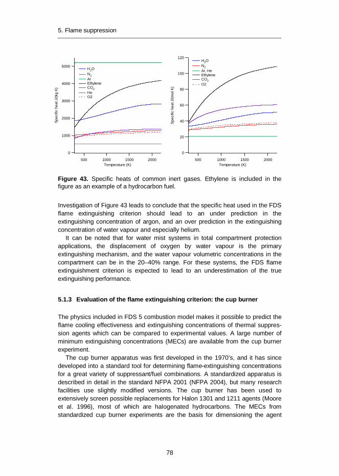
5. Flame suppression
78
Figure 43. Specific heats of common inert gases. Ethylene is included in the figure as an example of a hydrocarbon fuel.
Investigation of Figure 43 leads to conclude that the specific heat used in the FDS flame extinguishing criterion should lead to an under prediction in the extinguishing concentration of argon, and an over prediction in the extinguishing concentration of water vapour and especially helium.
It can be noted that for water mist systems in total compartment protection applications, the displacement of oxygen by water vapour is the primary extinguishing mechanism, and the water vapour volumetric concentrations in the compartment can be in the 20–40% range. For these systems, the FDS flame extinguishment criterion is expected to lead to an underestimation of the true extinguishing performance.
5.1.3 Evaluation of the flame extinguishing criterion: the cup burner
The physics included in FDS 5 combustion model makes it possible to predict the flame cooling effectiveness and extinguishing concentrations of thermal suppres-sion agents which can be compared to experimental values. A large number of minimum extinguishing concentrations (MECs) are available from the cup burner experiment.
The cup burner apparatus was first developed in the 1970’s, and it has since developed into a standard tool for determining flame-extinguishing concentrations for a great variety of suppressant/fuel combinations. A standardized apparatus is described in detail in the standard NFPA 2001 (NFPA 2004), but many research facilities use slightly modified versions. The cup burner has been used to extensively screen possible replacements for Halon 1301 and 1211 agents (Moore et al. 1996), most of which are halogenated hydrocarbons. The MECs from standardized cup burner experiments are the basis for dimensioning the agent
5000
4000
3000
2000
1000
0
Spec
ific
heat
J/(k
g K)
200015001000500Temperature (K)
H2O N2 Ar Ethylene CO2 He O2
120
100
80
60
40
20
0
Spec
ific
heat
J/(m
ol K
)
200015001000500Temperature (K)
H2O N2 Ar, He Ethylene CO2 O2

5. Flame suppression
79
containers for full-scale clean agent fire-extinguishing systems. Although many other laboratory-scale burners exist for determining MEC, it is often stated that the low-strain co-flow diffusion flame of the cup burner is a close representation of the diffusion flames in real fires.
The cup burner consists of a vertical round chimney 533 mm ± 10 mm in height and 85 mm ± 2 mm in inner diameter. An air-agent mixture is admitted to the chimney through a diffuser at the bottom of the chimney. A round fuel cup 28 31 mm in outer diameter and 1 2 mm wall thickness is on the axis of the chimney such that the rim of the cup is 235 mm above the chimney bottom.
To save on CPU time, only a part of the apparatus was modelled with FDS. An axisymmetric two-dimensional grid was used with a spatial resolution of 0.5 mm. There were 84 cells in the radial direction, and 480 cells in the axial direction. The FDS model was run in the DNS mode. The oxidizer inflow boundary was located 85 mm below the fuel inflow boundary. The cup was 14 mm in inner diameter. The rim of the cup was 1mm thick and 1 mm high. A surface temperature of 300ºC was applied to the rim. The chimney wall was a non-reacting solid surface with a fixed wall temperature of 20ºC.
The oxidizer inflow boundary was a simple inflow vent pushing a mixture of dry air and a gaseous suppressant into the chimney at 20ºC (ambient) temperature. The mass fraction of the suppressant could be ramped up as a function of time to mimic the actual cup burner experiment. Typically, the agent concentration was zero for a pre-burn time of a few seconds to allow for the flame to develop. Then, the agent concentration was increased to a level slightly below the extinguishing concentration, and ramped up over a time of about 30 seconds to a value that ensured flame extinguishment. For methane, the oxidizer inflow velocity was set to 0.107 m/s to give a volumetric flow rate of 36 L/min in the chimney. For heptane, the oxidizer inflow velocity was 0.118 m/s for a flow rate of 39 L/min. These velocities and flow rates are typical for the cup burner experiment, and correspond to the so-called ‘plateau region’ in a plot of the MEC vs. velocity for both gaseous and liquid fuels. In this region, the experimental MEC values are practically independent of the flow velocity (NFPA 2004).
For methane, the fuel inflow boundary was a simple inflow vent with a normal velocity of 0.92 cm/s for an oxidizer to fuel velocity ratio of 11.6:1. For heptane, a liquid evaporation model was used, where the evaporation rate of the fuel is governed by the Clausius-Clapeyron equation. With 0.5 mm cell size, the cup diameter is spanned by 56 cells.
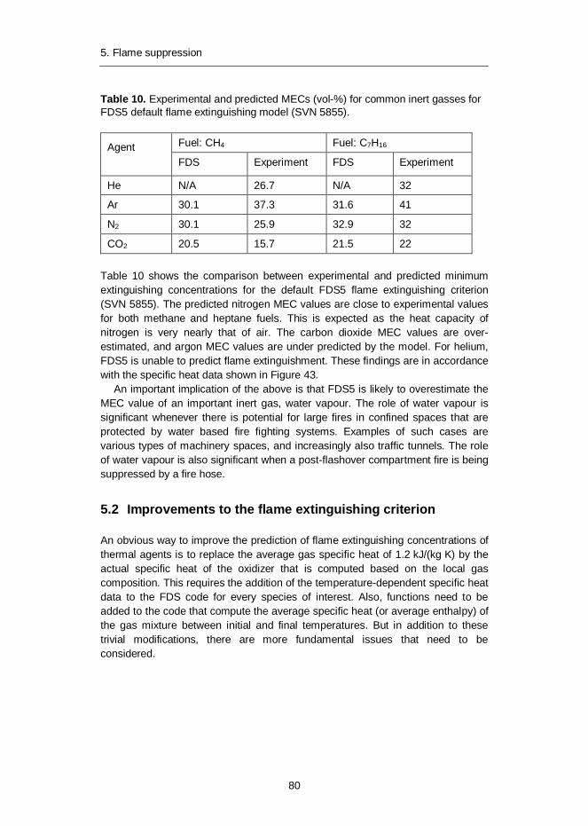
5. Flame suppression
80
Table 10. Experimental and predicted MECs (vol-%) for common inert gasses for FDS5 default flame extinguishing model (SVN 5855).
Agent Fuel: CH4 Fuel: C7H16
FDS Experiment FDS Experiment
He N/A 26.7 N/A 32
Ar 30.1 37.3 31.6 41
N2 30.1 25.9 32.9 32
CO2 20.5 15.7 21.5 22 Table 10 shows the comparison between experimental and predicted minimum extinguishing concentrations for the default FDS5 flame extinguishing criterion (SVN 5855). The predicted nitrogen MEC values are close to experimental values for both methane and heptane fuels. This is expected as the heat capacity of nitrogen is very nearly that of air. The carbon dioxide MEC values are over-estimated, and argon MEC values are under predicted by the model. For helium, FDS5 is unable to predict flame extinguishment. These findings are in accordance with the specific heat data shown in Figure 43.
An important implication of the above is that FDS5 is likely to overestimate the MEC value of an important inert gas, water vapour. The role of water vapour is significant whenever there is potential for large fires in confined spaces that are protected by water based fire fighting systems. Examples of such cases are various types of machinery spaces, and increasingly also traffic tunnels. The role of water vapour is also significant when a post-flashover compartment fire is being suppressed by a fire hose.
5.2 Improvements to the flame extinguishing criterion
An obvious way to improve the prediction of flame extinguishing concentrations of thermal agents is to replace the average gas specific heat of 1.2 kJ/(kg K) by the actual specific heat of the oxidizer that is computed based on the local gas composition. This requires the addition of the temperature-dependent specific heat data to the FDS code for every species of interest. Also, functions need to be added to the code that compute the average specific heat (or average enthalpy) of the gas mixture between initial and final temperatures. But in addition to these trivial modifications, there are more fundamental issues that need to be considered.

5. Flame suppression
81
5.2.1 Enthalpy calculation
Firstly, in textbook examples of combustion reactions the oxidation reaction is written first, followed by the enthalpy released by this reaction. It would therefore be tempting to compute the enthalpy increase for a gas composition after reaction. This is however not practical in the numerical implementation, as a reverse reaction would be needed in case the enthalpy increase is not sufficient. In reality, combustion is a complex series of chemical reactions that release various amounts of energy on the way. These are not however suitable for a lumped species combustion model. Numerically the most convenient path is to take the local gas composition before reaction and to check whether the enthalpy due to a potential reaction could rise the temperature of the unreacted gas mixture above a critical threshold temperature. This requires knowledge of the fuel specific heat data. Thermodynamically all these reaction paths are equivalent, because enthalpy is a thermodynamic state function, and for state functions, Hess’s Law states that the difference between state functions in the final and initial states (such as initial and final temperatures) is independent of the path between those states.
5.2.2 Stoichiometry
Secondly, it must be decided whether the enthalpy calculation is to be done for a stoichiometric mixture or for the true gas mixture in the cell. At this point it should be borne in mind that the lumped species combustion model in FDS is fundamentally designed for large-scale simulations where the spatial resolutions of 0.1 m–0.5 m are typical, i.e. much larger than the real flame sheet. The energy released by combustion in a given cell is distributed throughout the entire cell resulting in gas temperatures that are below true flame temperatures. Therefore, if the entire mass of gas in a large cell would be taken into account when determining the flame extinguishing criterion, little or no combustion would occur. For this reason, the extinguishing concentration does not consider the entire gas in a cell, but rather a portion of the gas in a cell that forms a stoichiometric mixture of fuel and oxidizer. Formally, the amount of fuel participating in combustion is obtained as
(28)
and the amount of oxidizer is obtained as
(29)
In the above formula, oxidizer is the cell gas mixture excluding fuel.
FOOFF rYYMINY /2,
FOO
FFOX r
YYYY /2
1
5. Flame suppression
82
5.2.3 Activation energy
Thirdly, it is noted that whenever fuel and oxidizer co-exist in a cell in such proportions that combustion would be possible based on the flame extinguishment criterion, it occurs spontaneously. This is a conscious choice by the FDS developers to make the model more user-friendly. In reality, most combustion reactions are activated chemical reactions. Due to the presence of an activation energy, combustion needs an external energy source, such as a spark, or the system must have sufficient internal energy (temperature) to initiate combustion. Conversely, without an activation energy, it would be difficult to completely extinguish flames which may lead to unphysical results. For example, when simulating under ventilated compartment fires, residual flames are often found around ventilation openings where temperature is close to ambient and where unburnt fuel is being convected through the vent. For the purpose of cup burner simulations, a new parameter, auto ignition temperature, was added to the reaction line. It prevents combustion in cells where the local gas temperature is below auto ignition temperature (AIT) regardless of the gas composition. It should be noted however, that this approach requires a spatial resolution that resolves true flame temperatures, i.e. DNS calculations. For coarse grid simulations, it is expected that the use of AIT would lead to unphysically small combustion efficiencies.
5.2.4 Cell surroundings
Finally, it should be evaluated whether there is a need to check the extinguishing criterion in the nearest-neighbour cells when deciding whether the current cell is allowed to react or not. For this, MEC values were computed for He, Ar, N2 and CO2 and for methane and n-heptane fuels using three different versions of the model, where extinguishment was evaluated based on the composition of
1. current cell only 2. current cell and six nearest-neighbour cells, and 3. current cell and all nearest-neighbour cells in the upwind direction.
The purpose of model 3 was to put special emphasis on the oxidizer stream that was convectively supplying oxygen to the flame. Denoting the gas velocity in the current cell by cv and in the neighbouring cell by nv a cell was considered to be in the upwind direction if
(30) 0nc vv
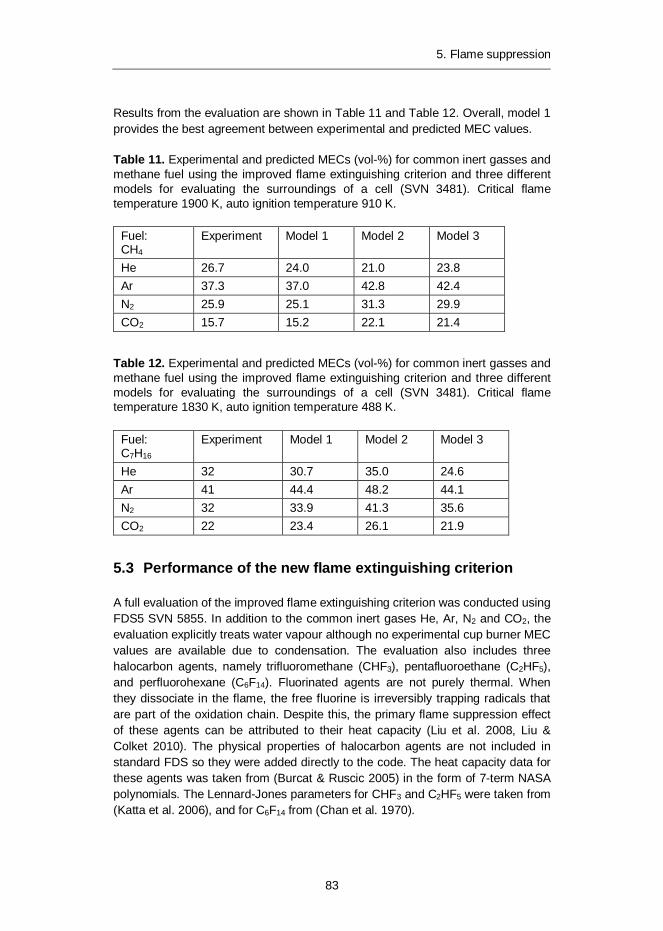
5. Flame suppression
83
Results from the evaluation are shown in Table 11 and Table 12. Overall, model 1 provides the best agreement between experimental and predicted MEC values.
Table 11. Experimental and predicted MECs (vol-%) for common inert gasses and methane fuel using the improved flame extinguishing criterion and three different models for evaluating the surroundings of a cell (SVN 3481). Critical flame temperature 1900 K, auto ignition temperature 910 K.
Fuel: CH4
Experiment Model 1 Model 2 Model 3
He 26.7 24.0 21.0 23.8 Ar 37.3 37.0 42.8 42.4 N2 25.9 25.1 31.3 29.9 CO2 15.7 15.2 22.1 21.4
Table 12. Experimental and predicted MECs (vol-%) for common inert gasses and methane fuel using the improved flame extinguishing criterion and three different models for evaluating the surroundings of a cell (SVN 3481). Critical flame temperature 1830 K, auto ignition temperature 488 K.
Fuel: C7H16
Experiment Model 1 Model 2 Model 3
He 32 30.7 35.0 24.6 Ar 41 44.4 48.2 44.1 N2 32 33.9 41.3 35.6 CO2 22 23.4 26.1 21.9
5.3 Performance of the new flame extinguishing criterion
A full evaluation of the improved flame extinguishing criterion was conducted using FDS5 SVN 5855. In addition to the common inert gases He, Ar, N2 and CO2, the evaluation explicitly treats water vapour although no experimental cup burner MEC values are available due to condensation. The evaluation also includes three halocarbon agents, namely trifluoromethane (CHF3), pentafluoroethane (C2HF5), and perfluorohexane (C6F14). Fluorinated agents are not purely thermal. When they dissociate in the flame, the free fluorine is irreversibly trapping radicals that are part of the oxidation chain. Despite this, the primary flame suppression effect of these agents can be attributed to their heat capacity (Liu et al. 2008, Liu & Colket 2010). The physical properties of halocarbon agents are not included in standard FDS so they were added directly to the code. The heat capacity data for these agents was taken from (Burcat & Ruscic 2005) in the form of 7-term NASA polynomials. The Lennard-Jones parameters for CHF3 and C2HF5 were taken from (Katta et al. 2006), and for C6F14 from (Chan et al. 1970).
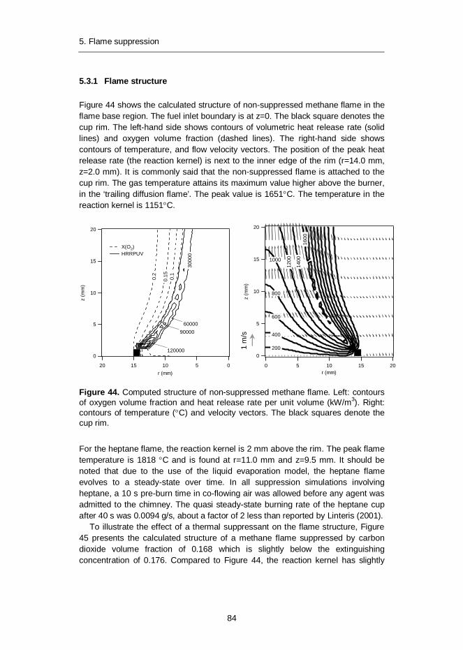
5. Flame suppression
84
5.3.1 Flame structure
Figure 44 shows the calculated structure of non-suppressed methane flame in the flame base region. The fuel inlet boundary is at z=0. The black square denotes the cup rim. The left-hand side shows contours of volumetric heat release rate (solid lines) and oxygen volume fraction (dashed lines). The right-hand side shows contours of temperature, and flow velocity vectors. The position of the peak heat release rate (the reaction kernel) is next to the inner edge of the rim (r=14.0 mm, z=2.0 mm). It is commonly said that the non-suppressed flame is attached to the cup rim. The gas temperature attains its maximum value higher above the burner, in the ‘trailing diffusion flame’. The peak value is 1651 C. The temperature in the reaction kernel is 1151 C.
Figure 44. Computed structure of non-suppressed methane flame. Left: contours of oxygen volume fraction and heat release rate per unit volume (kW/m3). Right: contours of temperature ( C) and velocity vectors. The black squares denote the cup rim.
For the heptane flame, the reaction kernel is 2 mm above the rim. The peak flame temperature is 1818 C and is found at r=11.0 mm and z=9.5 mm. It should be noted that due to the use of the liquid evaporation model, the heptane flame evolves to a steady-state over time. In all suppression simulations involving heptane, a 10 s pre-burn time in co-flowing air was allowed before any agent was admitted to the chimney. The quasi steady-state burning rate of the heptane cup after 40 s was 0.0094 g/s, about a factor of 2 less than reported by Linteris (2001).
To illustrate the effect of a thermal suppressant on the flame structure, Figure 45 presents the calculated structure of a methane flame suppressed by carbon dioxide volume fraction of 0.168 which is slightly below the extinguishing concentration of 0.176. Compared to Figure 44, the reaction kernel has slightly
20
15
10
5
0
z (m
m)
20 15 10 5 0r (mm)
300
00
0.2
0.1
5 0
.1
120000
90000 60000
X(O2) HRRPUV
20
15
10
5
0
z (m
m)
20151050r (mm)
200
160
0 1
400
120
0 1000
800
600
400
1 m
/s
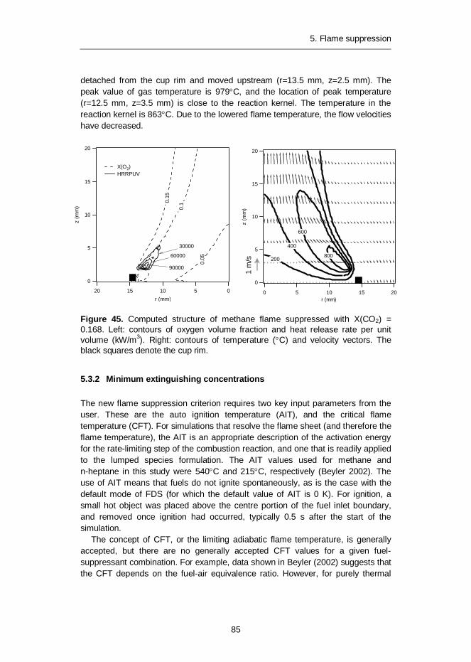
5. Flame suppression
85
detached from the cup rim and moved upstream (r=13.5 mm, z=2.5 mm). The peak value of gas temperature is 979 C, and the location of peak temperature (r=12.5 mm, z=3.5 mm) is close to the reaction kernel. The temperature in the reaction kernel is 863 C. Due to the lowered flame temperature, the flow velocities have decreased.
Figure 45. Computed structure of methane flame suppressed with X(CO2) = 0.168. Left: contours of oxygen volume fraction and heat release rate per unit volume (kW/m3). Right: contours of temperature ( C) and velocity vectors. The black squares denote the cup rim.
5.3.2 Minimum extinguishing concentrations
The new flame suppression criterion requires two key input parameters from the user. These are the auto ignition temperature (AIT), and the critical flame temperature (CFT). For simulations that resolve the flame sheet (and therefore the flame temperature), the AIT is an appropriate description of the activation energy for the rate-limiting step of the combustion reaction, and one that is readily applied to the lumped species formulation. The AIT values used for methane and n-heptane in this study were 540 C and 215 C, respectively (Beyler 2002). The use of AIT means that fuels do not ignite spontaneously, as is the case with the default mode of FDS (for which the default value of AIT is 0 K). For ignition, a small hot object was placed above the centre portion of the fuel inlet boundary, and removed once ignition had occurred, typically 0.5 s after the start of the simulation.
The concept of CFT, or the limiting adiabatic flame temperature, is generally accepted, but there are no generally accepted CFT values for a given fuel-suppressant combination. For example, data shown in Beyler (2002) suggests that the CFT depends on the fuel-air equivalence ratio. However, for purely thermal
20
15
10
5
0
z (m
m)
20 15 10 5 0r (mm)
30000
0.1
5
0.1
90000
60000
X(O2) HRRPUV
0.0
5
20
15
10
5
0
z (m
m)
20151050r (mm)
200 800
600
400 1
m/s
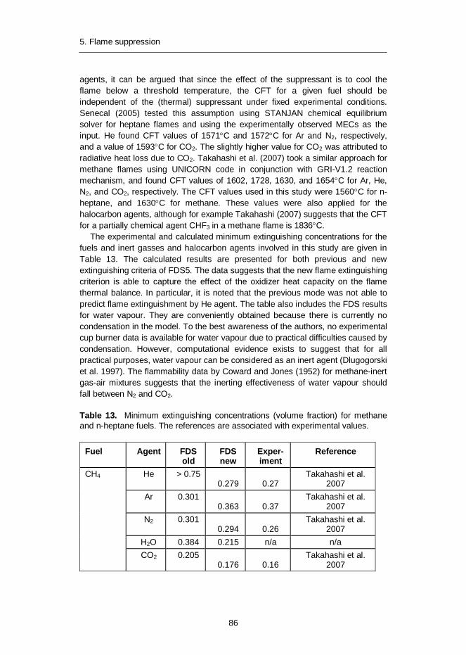
5. Flame suppression
86
agents, it can be argued that since the effect of the suppressant is to cool the flame below a threshold temperature, the CFT for a given fuel should be independent of the (thermal) suppressant under fixed experimental conditions. Senecal (2005) tested this assumption using STANJAN chemical equilibrium solver for heptane flames and using the experimentally observed MECs as the input. He found CFT values of 1571 C and 1572 C for Ar and N2, respectively, and a value of 1593 C for CO2. The slightly higher value for CO2 was attributed to radiative heat loss due to CO2. Takahashi et al. (2007) took a similar approach for methane flames using UNICORN code in conjunction with GRI-V1.2 reaction mechanism, and found CFT values of 1602, 1728, 1630, and 1654 C for Ar, He, N2, and CO2, respectively. The CFT values used in this study were 1560 C for n-heptane, and 1630 C for methane. These values were also applied for the halocarbon agents, although for example Takahashi (2007) suggests that the CFT for a partially chemical agent CHF3 in a methane flame is 1836 C.
The experimental and calculated minimum extinguishing concentrations for the fuels and inert gasses and halocarbon agents involved in this study are given in Table 13. The calculated results are presented for both previous and new extinguishing criteria of FDS5. The data suggests that the new flame extinguishing criterion is able to capture the effect of the oxidizer heat capacity on the flame thermal balance. In particular, it is noted that the previous mode was not able to predict flame extinguishment by He agent. The table also includes the FDS results for water vapour. They are conveniently obtained because there is currently no condensation in the model. To the best awareness of the authors, no experimental cup burner data is available for water vapour due to practical difficulties caused by condensation. However, computational evidence exists to suggest that for all practical purposes, water vapour can be considered as an inert agent (Dlugogorski et al. 1997). The flammability data by Coward and Jones (1952) for methane-inert gas-air mixtures suggests that the inerting effectiveness of water vapour should fall between N2 and CO2.
Table 13. Minimum extinguishing concentrations (volume fraction) for methane and n-heptane fuels. The references are associated with experimental values.
Fuel Agent FDS old
FDS new
Exper-iment
Reference
CH4 He > 0.75 0.279 0.27
Takahashi et al. 2007
Ar 0.301 0.363 0.37
Takahashi et al. 2007
N2 0.301 0.294 0.26
Takahashi et al. 2007
H2O 0.384 0.215 n/a n/a CO2 0.205
0.176 0.16 Takahashi et al.
2007
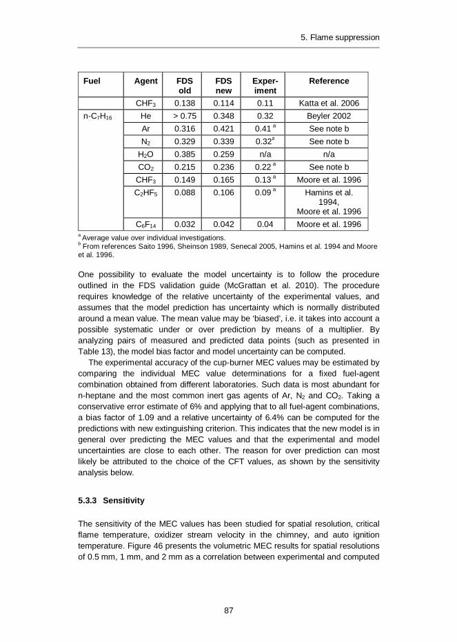
5. Flame suppression
87
Fuel Agent FDS old
FDS new
Exper-iment
Reference
CHF3 0.138 0.114 0.11 Katta et al. 2006 n-C7H16 He > 0.75 0.348 0.32 Beyler 2002
Ar 0.316 0.421 0.41 a See note b N2 0.329 0.339 0.32a See note b
H2O 0.385 0.259 n/a n/a CO2 0.215 0.236 0.22 a See note b
CHF3 0.149 0.165 0.13 a Moore et al. 1996 C2HF5 0.088 0.106 0.09 a Hamins et al.
1994, Moore et al. 1996
C6F14 0.032 0.042 0.04 Moore et al. 1996 a Average value over individual investigations. b From references Saito 1996, Sheinson 1989, Senecal 2005, Hamins et al. 1994 and Moore et al. 1996. One possibility to evaluate the model uncertainty is to follow the procedure outlined in the FDS validation guide (McGrattan et al. 2010). The procedure requires knowledge of the relative uncertainty of the experimental values, and assumes that the model prediction has uncertainty which is normally distributed around a mean value. The mean value may be ‘biased’, i.e. it takes into account a possible systematic under or over prediction by means of a multiplier. By analyzing pairs of measured and predicted data points (such as presented in Table 13), the model bias factor and model uncertainty can be computed.
The experimental accuracy of the cup-burner MEC values may be estimated by comparing the individual MEC value determinations for a fixed fuel-agent combination obtained from different laboratories. Such data is most abundant for n-heptane and the most common inert gas agents of Ar, N2 and CO2. Taking a conservative error estimate of 6% and applying that to all fuel-agent combinations, a bias factor of 1.09 and a relative uncertainty of 6.4% can be computed for the predictions with new extinguishing criterion. This indicates that the new model is in general over predicting the MEC values and that the experimental and model uncertainties are close to each other. The reason for over prediction can most likely be attributed to the choice of the CFT values, as shown by the sensitivity analysis below.
5.3.3 Sensitivity
The sensitivity of the MEC values has been studied for spatial resolution, critical flame temperature, oxidizer stream velocity in the chimney, and auto ignition temperature. Figure 46 presents the volumetric MEC results for spatial resolutions of 0.5 mm, 1 mm, and 2 mm as a correlation between experimental and computed
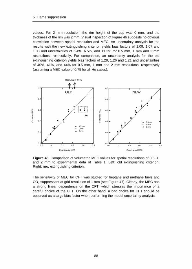
5. Flame suppression
88
values. For 2 mm resolution, the rim height of the cup was 0 mm, and the thickness of the rim was 2 mm. Visual inspection of Figure 46 suggests no obvious correlation between spatial resolution and MEC. An uncertainty analysis for the results with the new extinguishing criterion yields bias factors of 1.09, 1.07 and 1.03 and uncertainties of 6.4%, 6.5%, and 11.2% for 0.5 mm, 1 mm and 2 mm resolutions, respectively. For comparison, an uncertainty analysis for the old extinguishing criterion yields bias factors of 1.28, 1.26 and 1.21 and uncertainties of 40%, 41%, and 44% for 0.5 mm, 1 mm and 2 mm resolutions, respectively (assuming a MEC value of 0.75 for all He cases).
Figure 46. Comparison of volumetric MEC values for spatial resolutions of 0.5, 1, and 2 mm to experimental data of Table 1. Left: old extinguishing criterion. Right: new extinguishing criterion.
The sensitivity of MEC for CFT was studied for heptane and methane fuels and CO2 suppressant at grid resolution of 1 mm (see Figure 47). Clearly, the MEC has a strong linear dependence on the CFT, which stresses the importance of a careful choice of the CFT. On the other hand, a bad choice for CFT should be observed as a large bias factor when performing the model uncertainty analysis.
0.5
0.4
0.3
0.2
0.1
0.0
Com
pute
d M
EC
0.50.40.30.20.10.0
Experimental MEC
0.5 mm 1 mm 2 mm
0.5
0.4
0.3
0.2
0.1
0.0
Com
pute
d M
EC
0.50.40.30.20.10.0
Experimental MEC
0.5 mm 1 mm 2 mm
He: MEC > 0.75
OLD NEW
Ar
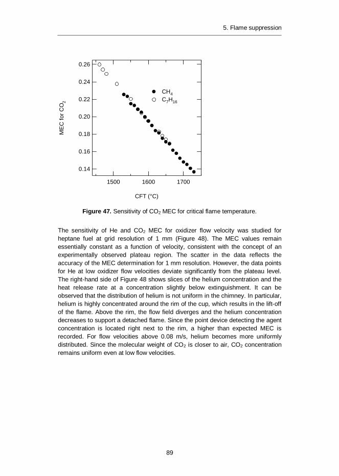
5. Flame suppression
89
Figure 47. Sensitivity of CO2 MEC for critical flame temperature.
The sensitivity of He and CO2 MEC for oxidizer flow velocity was studied for heptane fuel at grid resolution of 1 mm (Figure 48). The MEC values remain essentially constant as a function of velocity, consistent with the concept of an experimentally observed plateau region. The scatter in the data reflects the accuracy of the MEC determination for 1 mm resolution. However, the data points for He at low oxidizer flow velocities deviate significantly from the plateau level. The right-hand side of Figure 48 shows slices of the helium concentration and the heat release rate at a concentration slightly below extinguishment. It can be observed that the distribution of helium is not uniform in the chimney. In particular, helium is highly concentrated around the rim of the cup, which results in the lift-off of the flame. Above the rim, the flow field diverges and the helium concentration decreases to support a detached flame. Since the point device detecting the agent concentration is located right next to the rim, a higher than expected MEC is recorded. For flow velocities above 0.08 m/s, helium becomes more uniformly distributed. Since the molecular weight of CO2 is closer to air, CO2 concentration remains uniform even at low flow velocities.
0.26
0.24
0.22
0.20
0.18
0.16
0.14
ME
C fo
r CO
2
170016001500
CFT (°C)
CH4 C7H16
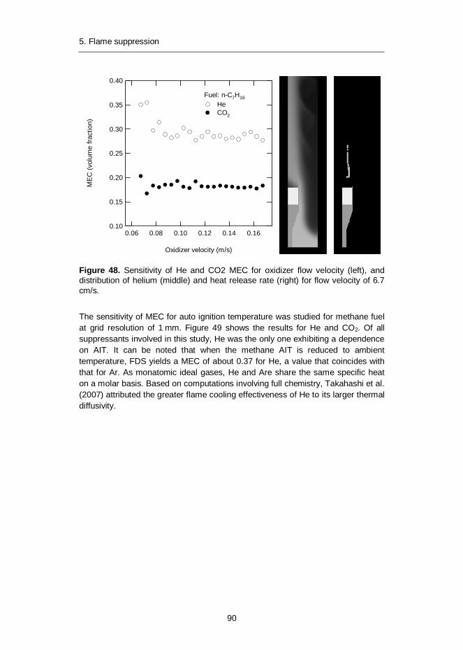
5. Flame suppression
90
Figure 48. Sensitivity of He and CO2 MEC for oxidizer flow velocity (left), and distribution of helium (middle) and heat release rate (right) for flow velocity of 6.7 cm/s.
The sensitivity of MEC for auto ignition temperature was studied for methane fuel at grid resolution of 1 mm. Figure 49 shows the results for He and CO2. Of all suppressants involved in this study, He was the only one exhibiting a dependence on AIT. It can be noted that when the methane AIT is reduced to ambient temperature, FDS yields a MEC of about 0.37 for He, a value that coincides with that for Ar. As monatomic ideal gases, He and Are share the same specific heat on a molar basis. Based on computations involving full chemistry, Takahashi et al. (2007) attributed the greater flame cooling effectiveness of He to its larger thermal diffusivity.
0.40
0.35
0.30
0.25
0.20
0.15
0.10
MEC
(vol
ume
fract
ion)
0.160.140.120.100.080.06
Oxidizer velocity (m/s)
Fuel: n-C7H16 He CO2
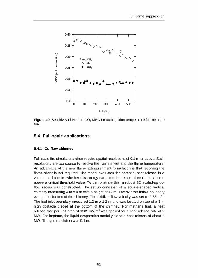
5. Flame suppression
91
Figure 49. Sensitivity of He and CO2 MEC for auto ignition temperature for methane fuel.
5.4 Full-scale applications
5.4.1 Co-flow chimney
Full-scale fire simulations often require spatial resolutions of 0.1 m or above. Such resolutions are too coarse to resolve the flame sheet and the flame temperature. An advantage of the new flame extinguishment formulation is that resolving the flame sheet is not required. The model evaluates the potential heat release in a volume and checks whether this energy can raise the temperature of the volume above a critical threshold value. To demonstrate this, a robust 3D scaled-up co-flow set-up was constructed. The set-up consisted of a square-shaped vertical chimney measuring 4 m x 4 m with a height of 12 m. The oxidizer inflow boundary was at the bottom of the chimney. The oxidizer flow velocity was set to 0.83 m/s. The fuel inlet boundary measured 1.2 m x 1.2 m and was located on top of a 3 m high obstacle placed at the bottom of the chimney. For methane fuel, a heat release rate per unit area of 1389 kW/m2 was applied for a heat release rate of 2 MW. For heptane, the liquid evaporation model yielded a heat release of about 4 MW. The grid resolution was 0.1 m.
0.40
0.35
0.30
0.25
0.20
0.15
0.10
ME
C (v
olum
e fra
ctio
n)
5004003002001000
AIT (°C)
Fuel: CH4 He CO2
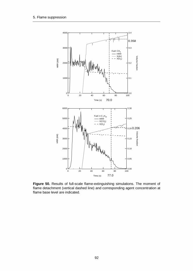
5. Flame suppression
92
Figure 50. Results of full-scale flame-extinguishing simulations. The moment of flame detachment (vertical dashed line) and corresponding agent concentration at flame base level are indicated.
4000
3000
2000
1000
0
HR
R (k
W)
100806040200
Time (s)
0.4
0.3
0.2
0.1
0.0
Volume fraction
Fuel: CH4 HRR X(Ar) X(O2)
6000
5000
4000
3000
2000
1000
0
HR
R (k
W)
100806040200
Time (s)
0.30
0.25
0.20
0.15
0.10
0.05
0.00
Volume fraction
Fuel: n-C 7H16 HRR X(CO2) X(O2)
70.0
0.358
77.0
0.206
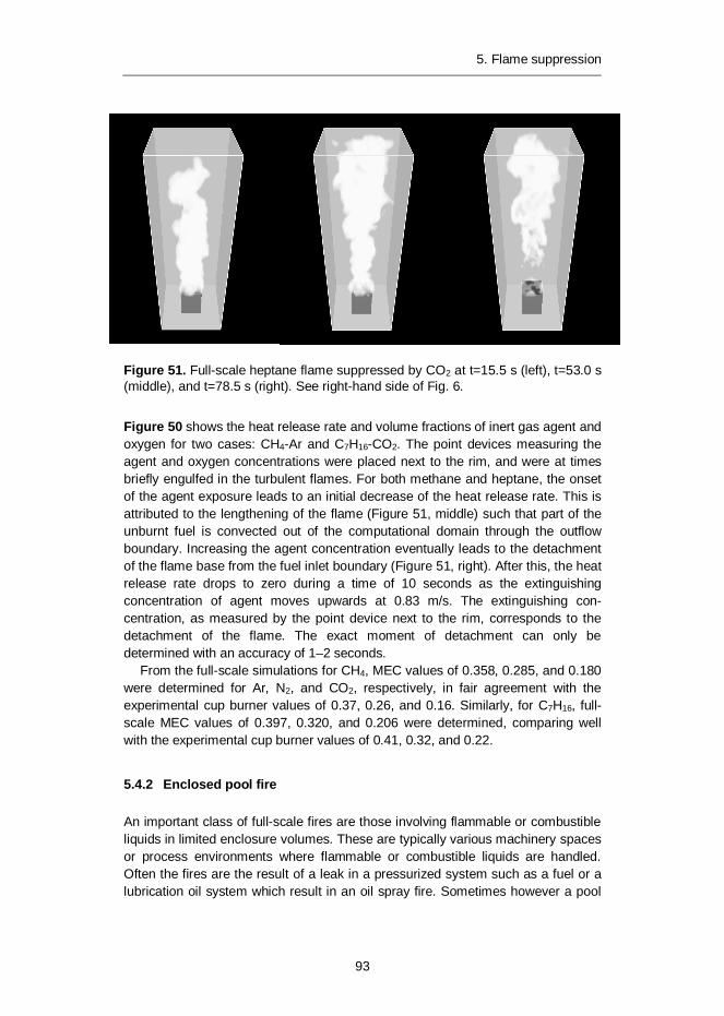
5. Flame suppression
93
Figure 51. Full-scale heptane flame suppressed by CO2 at t=15.5 s (left), t=53.0 s (middle), and t=78.5 s (right). See right-hand side of Fig. 6.
Figure 50 shows the heat release rate and volume fractions of inert gas agent and oxygen for two cases: CH4-Ar and C7H16-CO2. The point devices measuring the agent and oxygen concentrations were placed next to the rim, and were at times briefly engulfed in the turbulent flames. For both methane and heptane, the onset of the agent exposure leads to an initial decrease of the heat release rate. This is attributed to the lengthening of the flame (Figure 51, middle) such that part of the unburnt fuel is convected out of the computational domain through the outflow boundary. Increasing the agent concentration eventually leads to the detachment of the flame base from the fuel inlet boundary (Figure 51, right). After this, the heat release rate drops to zero during a time of 10 seconds as the extinguishing concentration of agent moves upwards at 0.83 m/s. The extinguishing con-centration, as measured by the point device next to the rim, corresponds to the detachment of the flame. The exact moment of detachment can only be determined with an accuracy of 1–2 seconds.
From the full-scale simulations for CH4, MEC values of 0.358, 0.285, and 0.180 were determined for Ar, N2, and CO2, respectively, in fair agreement with the experimental cup burner values of 0.37, 0.26, and 0.16. Similarly, for C7H16, full-scale MEC values of 0.397, 0.320, and 0.206 were determined, comparing well with the experimental cup burner values of 0.41, 0.32, and 0.22.
5.4.2 Enclosed pool fire
An important class of full-scale fires are those involving flammable or combustible liquids in limited enclosure volumes. These are typically various machinery spaces or process environments where flammable or combustible liquids are handled. Often the fires are the result of a leak in a pressurized system such as a fuel or a lubrication oil system which result in an oil spray fire. Sometimes however a pool

5. Flame suppression
94
fire may form on the floor level of such a space. The performance of fire extinguishing systems for machinery spaces are normally tested using a set of spray and pool fires and typically using a high flashpoint fuel such as diesel oil, and/or a low flashpoint fuel such as heptane. Practice has shown that often pool fires of low flashpoint liquids are the most difficult fires to extinguish. It is therefore of interest to see how the suppression and eventual extinguishment of a pool fire in an enclosure can be predicted by the flame extinguishment included in FDS.
There are a few well-documented and well instrumented test series performed to investigate the performance of water-based fire suppression systems in machinery spaces (Back et al. 2000, Arvidson & Hertzberg 2003). The VINNOVA test series (Arvidson & Hertzberg 2003) is particularly suitable for this work because many of the tests were conducted using obstructed heptane pool fires, and for some of these tests, a high pressure water mist system was used that was based on the nozzle technology involved in Chapter 2.
The VINNOVA test series was conducted in an enclosure measuring 8m x 12.5 m x 5 m (high) with a volume of 500 m3. The fire scenario chosen for this work was a round heptane pool with a diameter of 1.12 m and an area of 1.0 m2. The pool was filled with 50 litres of heptane on a 50 litre water bed such that the freeboard was 150 mm. The pool had a nominal heat release rate of 2 MW. The pool was placed on a scale positioned centrally on the floor of the test enclosure, and it was obstructed by a 4 mm thick steel plate measuring 2 m x 2 m and positioned 1 m above floor level. For the test simulated below, all ventilation openings in the enclosure were closed, and only allowed to act as pressure relief vents. The pre-burn time was 30 seconds.
The high pressure water mist system for the experiments was supplied by Marioff Corporation Oy and consisted of four ceiling mounted spray heads of the HI-FOG 1000 product family. At 70 bar pressure each spray head flowed about 15 l/min. The spray heads were installed with a 5.0 m spacing in the longitudinal direction and 2.5 m spacing in the transverse direction of the test enclosure.
The experiments were instrumented for gas and surface temperatures, gas concentrations (O2, CO2, CO, relative humidity), radiative heat fluxes, compart-ment pressure, mass loss rate of the pool, and the water pressure in the suppression system pipe work.
The FDS model of the test enclosure is shown in Figure 52. The spatial resolution of the model was 10 cm. The pool fire was modelled using the liquid evaporation model of FDS (boiling temperature 98ºC). The heat release rate per unit volume of the heptane combustion reaction was limited to 1000 kW/m3. The spray pattern for each spray head was constructed according to the spray head multiport configuration. Each spray was modeled as a 10 degree wide full cone. The FDS default droplet size distribution was used with a volume mean diameter of 80 m.
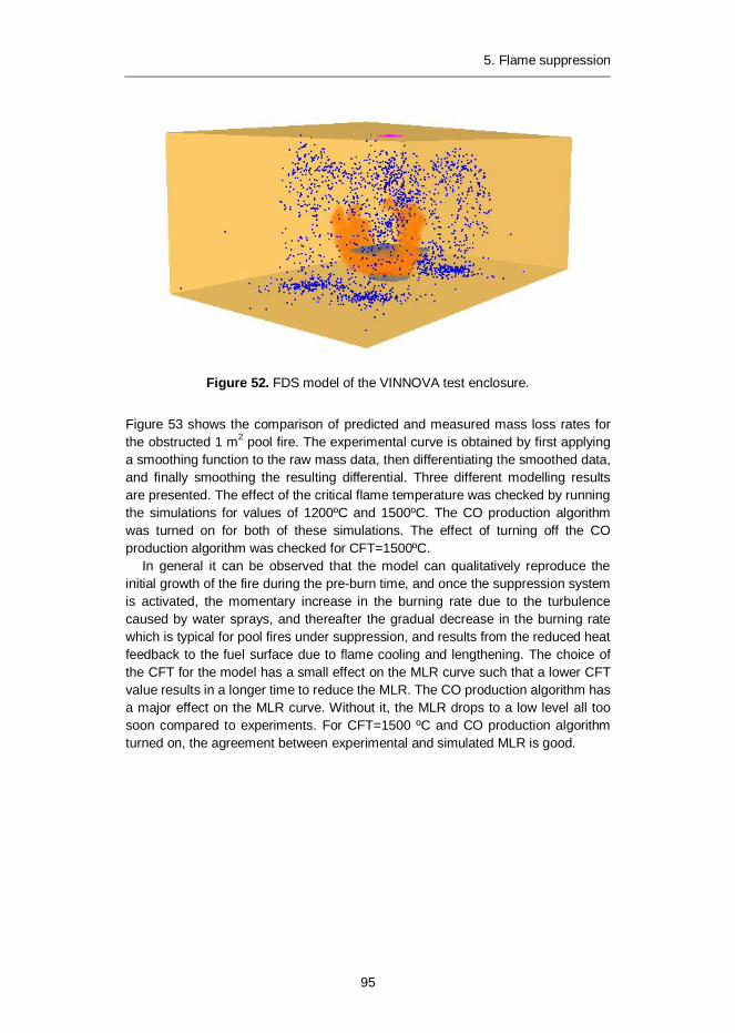
5. Flame suppression
95
Figure 52. FDS model of the VINNOVA test enclosure.
Figure 53 shows the comparison of predicted and measured mass loss rates for the obstructed 1 m2 pool fire. The experimental curve is obtained by first applying a smoothing function to the raw mass data, then differentiating the smoothed data, and finally smoothing the resulting differential. Three different modelling results are presented. The effect of the critical flame temperature was checked by running the simulations for values of 1200ºC and 1500ºC. The CO production algorithm was turned on for both of these simulations. The effect of turning off the CO production algorithm was checked for CFT=1500ºC.
In general it can be observed that the model can qualitatively reproduce the initial growth of the fire during the pre-burn time, and once the suppression system is activated, the momentary increase in the burning rate due to the turbulence caused by water sprays, and thereafter the gradual decrease in the burning rate which is typical for pool fires under suppression, and results from the reduced heat feedback to the fuel surface due to flame cooling and lengthening. The choice of the CFT for the model has a small effect on the MLR curve such that a lower CFT value results in a longer time to reduce the MLR. The CO production algorithm has a major effect on the MLR curve. Without it, the MLR drops to a low level all too soon compared to experiments. For CFT=1500 ºC and CO production algorithm turned on, the agreement between experimental and simulated MLR is good.
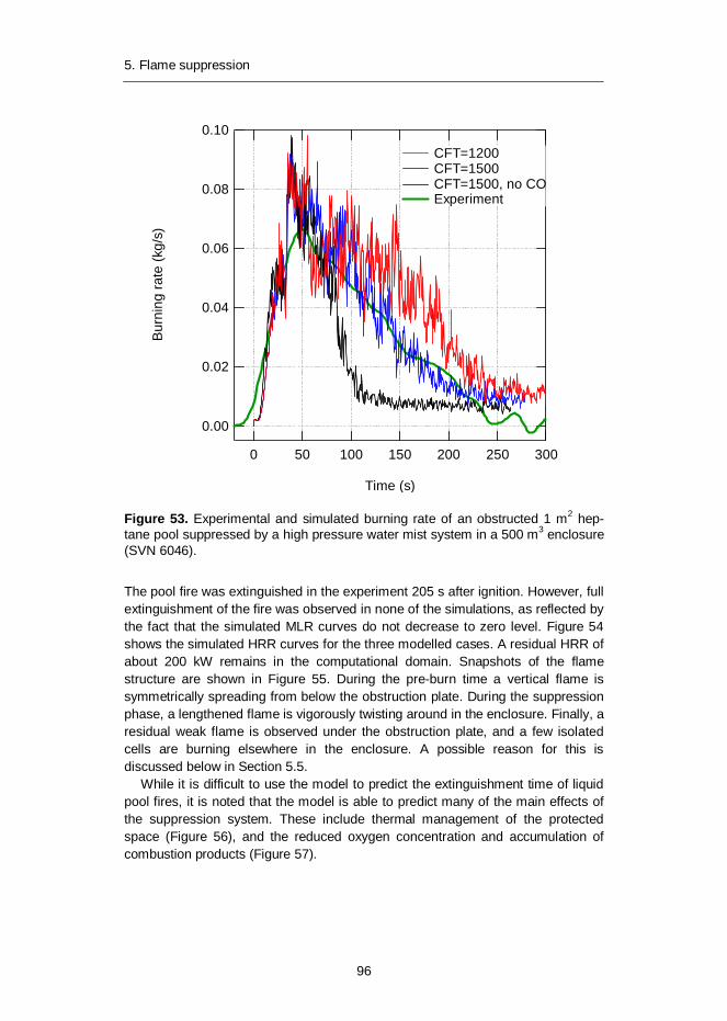
5. Flame suppression
96
Figure 53. Experimental and simulated burning rate of an obstructed 1 m2 hep-tane pool suppressed by a high pressure water mist system in a 500 m3 enclosure (SVN 6046).
The pool fire was extinguished in the experiment 205 s after ignition. However, full extinguishment of the fire was observed in none of the simulations, as reflected by the fact that the simulated MLR curves do not decrease to zero level. Figure 54 shows the simulated HRR curves for the three modelled cases. A residual HRR of about 200 kW remains in the computational domain. Snapshots of the flame structure are shown in Figure 55. During the pre-burn time a vertical flame is symmetrically spreading from below the obstruction plate. During the suppression phase, a lengthened flame is vigorously twisting around in the enclosure. Finally, a residual weak flame is observed under the obstruction plate, and a few isolated cells are burning elsewhere in the enclosure. A possible reason for this is discussed below in Section 5.5.
While it is difficult to use the model to predict the extinguishment time of liquid pool fires, it is noted that the model is able to predict many of the main effects of the suppression system. These include thermal management of the protected space (Figure 56), and the reduced oxygen concentration and accumulation of combustion products (Figure 57).
0.10
0.08
0.06
0.04
0.02
0.00
Bur
ning
rate
(kg/
s)
300250200150100500
Time (s)
CFT=1200 CFT=1500 CFT=1500, no CO Experiment
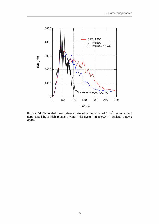
5. Flame suppression
97
Figure 54. Simulated heat release rate of an obstructed 1 m2 heptane pool suppressed by a high pressure water mist system in a 500 m3 enclosure (SVN 6046).
5000
4000
3000
2000
1000
0
HR
R (k
W)
300250200150100500
Time (s)
CFT=1200 CFT=1500 CFT=1500, no CO
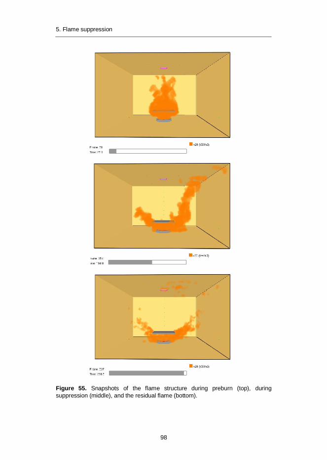
5. Flame suppression
98
Figure 55. Snapshots of the flame structure during preburn (top), during suppression (middle), and the residual flame (bottom).
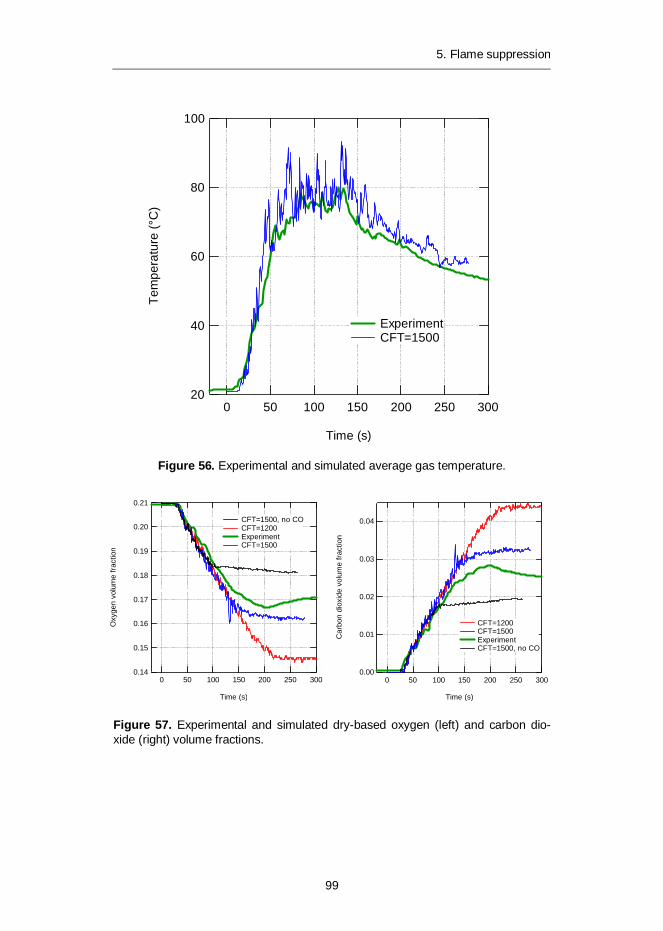
5. Flame suppression
99
Figure 56. Experimental and simulated average gas temperature.
Figure 57. Experimental and simulated dry-based oxygen (left) and carbon dio-xide (right) volume fractions.
100
80
60
40
20
Tem
pera
ture
(°C
)
300250200150100500
Time (s)
Experiment CFT=1500
0.21
0.20
0.19
0.18
0.17
0.16
0.15
0.14
Oxy
gen
volu
me
fract
ion
300250200150100500
Time (s)
CFT=1500, no CO CFT=1200 Experiment CFT=1500
0.04
0.03
0.02
0.01
0.00
Car
bon
diox
ide
volu
me
fract
ion
300250200150100500
Time (s)
CFT=1200 CFT=1500 Experiment CFT=1500, no CO
5. Flame suppression
100
5.5 Limits of validity
As discussed above in Section 5.2.2, the enthalpy calculation for evaluating cell combustion is performed for a stoichiometric mixture instead of taking into account the entire volume of gas in a cell. It is instructive therefore to evaluate whether this choice somehow limits the ability of FDS to predict flame extinguishment. One way to test the extinguishment criterion is to try to predict the flammability diagram of a ternary mixture of fuel, air, and diluent. Experimental flammability data is abundantly available. For this work, the tubular burner experiment is modelled, as reported in Liao et al. (1996).
The experimental tubular burner was a porous brass cylinder with an inner diameter of 30 mm and a length of 80 mm. A ternary mixture is injected radically through the porous cylinder from the outside towards the axis of the cylinder, resulting in a cylindrically symmetric flame with a circular cross section. Combustion products escape through both ends of the cylinder, which results in minimal heat losses in the post-flame region. A nitrogen shroud is applied at both ends of the cylinder to suppress diffusion flames that otherwise would block the view to the inside of the cylinder.
The tubular burner was modelled as a 2D axisymmetric domain with 1 mm spatial resolution, 15 cells in the radial direction and 100 cells in the axial direction. The ternary mixture inlet and the nitrogen shrouds were modelled as simple inflow vents on the boundary of the domain. Inflow velocity was set at 5 cm/s. Gravity vector was defined parallel to the radial direction to simulate a horizontally positioned burner. Direct numerical simulation was applied. An auto ignition temperature of 540ºC and a critical flame temperature of 1630ºC were applied for methane reaction.
Simulations were carried out to map the flammability diagram of CH4-Ar-air ternary mixture. The simulations were run in a similar manner to the experiments. First, for a given diluent concentration, a mixture was chosen that was close to the stoichiometric line on the flammability diagram to ensure that the mixture was flammable. The flame was allowed to stabilize for five seconds. Thereafter, the fuel concentration was ramped down to zero or up to 100% during 15 seconds depending on whether the lean or the rich flammability limit was searched.
The results from the simulations are shown in Figure 50 with the blue symbols. For comparison, the green curve is the experimental result by Liao et al. (1996). It is obvious that the flame suppression model is not able to predict the flammability diagram. In particular, the model is not able to predict the lower and upper flammability limits of methane in pure air. The error is particularly large on the fuel-rich branch where the model predicts that highly fuel-rich mixtures will undergo combustion. This error is a likely reason for the residual flames observed in the full-scale simulation of an enclosed pool fire discussed above in Section 5.4.2.
For comparison, the flammability limit was also mapped using a further modification to the extinguishment criterion that considered the entire volume of gas in a cell. The results are plotted in Figure 58 with red symbols. The agreement

5. Flame suppression
101
between experiment and simulation is much better in this case, and the major disagreement comes from the fact that the simulated result fail to predict the existence of a flame for diluent concentrations above X(Ar)=0.32. For reference, the cup-burner cases shown in Figurae 46 were run with 2 mm resolution and the extinction criterion considering the entire cell volume. The results are presented in Figure 59, suggesting that the MEC values are generally in agreement with experimental ones. However, the MEC for Ar/CH4 is 0.33 and thus smaller than the experimental value of 0.37. Further work will on the tubular burner model will be required to understand the model behaviour at high diluent concentrations.
Figure 58. Experimental and predicted flammability diagram of CH4-Ar-air ternary mixture.
0.5
0.4
0.3
0.2
0.1
0.0
Fuel
vol
ume
fract
ion
0.40.30.20.10.0
Argon volume fraction
Stoichiometric mixture Cell mixture Tubular burner

5. Flame suppression
102
Figure 59. Experimental and computed cup-burner MEC values for methane and heptane fuels and selected inert gas and halocarbon agents with an extinction criterion considering the entire gas volume in a cell.
0.5
0.4
0.3
0.2
0.1
0.0
Com
pute
d M
EC
0.50.40.30.20.10.0
Experimental MEC
2 mm
6. Suppressability of idle wooden pallets
103
6. Suppressability of idle wooden pallets
6.1 Pyrolysis of wood
Chemically, dry wood is composed of carbon (50%), hydrogen (6%) oxygen (44%) and trace amounts of nitrogen and inorganic compounds. These are combined to three natural polymers, cellulose, hemicellulose and lignin. The amount of cellulose is similar for hardwood and softwood, but softwood has more lignin and less hemicellulose than hardwood. Of the three compounds, lignin has the highest decomposition temperature, and it also releases the smallest fraction of volatile compounds (leading to a larger char residue).
In FDS, the burning rate of solids (or liquids) can be either prescribed or predicted. If the goal of the simulation is to predict the effect of water application to a burning surface on the burning rate of that surface, it is obviously desirable to try and use FDS to predict the burning rate. This requires detailed knowledge of the surface reactions leading to the release of combustible gasses.
Matala (2008) has performed a detailed study on estimating the input parameters required to describe the pyrolysis of non-charring and charring solids in fire simulation. The basic assumption behind the work is that given a solid composing of N material components, each with a density i and mass fraction Yi, the reaction rate converting component i to another substance (either an intermediate or a final product) can be written in Arrhenius form
RTEN
ii eAt
S
00
(31)
It should be noted that the Arrhenius form for the reaction rate is originally developed to describe gas-phase reactions, but it is widely used to describe any reactions whose rate exhibits a dependence on temperature. The problem of describing the pyrolysis of a solid material is then to define the reaction or reactions leading from virgin material to final products, and to obtain the kinetic parameters A, E, and NS for each of these reactions. Assuming this can be done, the next step is to compute the heat balance of the burning surface in order to define the surface temperature T. This requires knowledge of the thermal
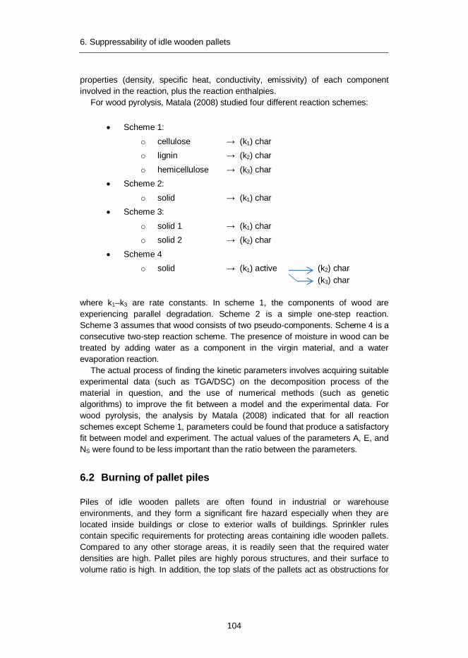
6. Suppressability of idle wooden pallets
104
properties (density, specific heat, conductivity, emissivity) of each component involved in the reaction, plus the reaction enthalpies.
For wood pyrolysis, Matala (2008) studied four different reaction schemes:
Scheme 1: o cellulose (k1) char o lignin (k2) char o hemicellulose (k3) char
Scheme 2: o solid (k1) char
Scheme 3: o solid 1 (k1) char o solid 2 (k2) char
Scheme 4 o solid (k1) active (k2) char
(k3) char where k1–k3 are rate constants. In scheme 1, the components of wood are experiencing parallel degradation. Scheme 2 is a simple one-step reaction. Scheme 3 assumes that wood consists of two pseudo-components. Scheme 4 is a consecutive two-step reaction scheme. The presence of moisture in wood can be treated by adding water as a component in the virgin material, and a water evaporation reaction.
The actual process of finding the kinetic parameters involves acquiring suitable experimental data (such as TGA/DSC) on the decomposition process of the material in question, and the use of numerical methods (such as genetic algorithms) to improve the fit between a model and the experimental data. For wood pyrolysis, the analysis by Matala (2008) indicated that for all reaction schemes except Scheme 1, parameters could be found that produce a satisfactory fit between model and experiment. The actual values of the parameters A, E, and NS were found to be less important than the ratio between the parameters.
6.2 Burning of pallet piles
Piles of idle wooden pallets are often found in industrial or warehouse environments, and they form a significant fire hazard especially when they are located inside buildings or close to exterior walls of buildings. Sprinkler rules contain specific requirements for protecting areas containing idle wooden pallets. Compared to any other storage areas, it is readily seen that the required water densities are high. Pallet piles are highly porous structures, and their surface to volume ratio is high. In addition, the top slats of the pallets act as obstructions for
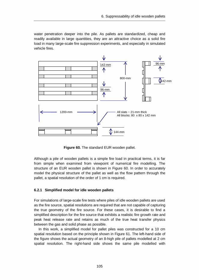
6. Suppressability of idle wooden pallets
105
water penetration deeper into the pile. As pallets are standardized, cheap and readily available in large quantities, they are an attractive choice as a solid fire load in many large-scale fire suppression experiments, and especially in simulated vehicle fires.
Figure 60. The standard EUR wooden pallet.
Although a pile of wooden pallets is a simple fire load in practical terms, it is far from simple when examined from viewpoint of numerical fire modelling. The structure of an EUR wooden pallet is shown in Figure 60. In order to accurately model the physical structure of the pallet as well as the flow pattern through the pallet, a spatial resolution of the order of 1 cm is required.
6.2.1 Simplified model for idle wooden pallets
For simulations of large-scale fire tests where piles of idle wooden pallets are used as the fire source, spatial resolutions are required that are not capable of capturing the true geometry of the fire source. For these cases, it is desirable to find a simplified description for the fire source that exhibits a realistic fire growth rate and peak heat release rate and retains as much of the true heat transfer physics between the gas and solid phase as possible.
In this work, a simplified model for pallet piles was constructed for a 10 cm spatial resolution based on the principle shown in Figure 61. The left-hand side of the figure shows the actual geometry of an 8-high pile of pallets modelled at 2 cm spatial resolution. The right-hand side shows the same pile modelled with
142-mm
142-mm
1200-mm
800-mm
144-mm
All slats ~ 21-mm thick All blocks: 80 x 80 x 142 mm
96-mm
96-mm

6. Suppressability of idle wooden pallets
106
obstacles conforming to 10 cm spatial resolution. The simplified model is designed to preserve some of the geometrical structure of the real pallet pile for the purpose of predicting both the fire spread and penetration of water into the pile.
Figure 61. The structure of a real (left) and simplified (right) pallet pile.
The surface area and solid volume of the simplified fire load are smaller than those of the real fire load. Also the physics of fuel pyrolysis and flame spread are simplified. The burning of the fuel is described by a heat release rate per unit area (HRRPUA). To conserve the potential peak HRR of the pallet pile (which assumes all surfaces are burning), the HRRPUA of the real material (typically 120 150 kW/m2 for softwood) should be corrected for the ratio of surface areas. However, the heat transport between gas and solid phases is based on the thermal properties of real wood to ensure that the heating of the material up to ignition temperature occurs at a realistic rate, and the ignition temperature is physically correct.
In FDS, the use of a HRRPUA to describe pyrolysis means by default that once a surface ignites, it emits fuel at a fixed pre-determined rate. It is however possible to change this behavior by adding a user-defined time dependence for the HRRPUA. Each appropriate wall cell will then follow this time dependence from the moment the said wall cell has ignited. It is in principle possible to take this time dependence for example from a cone calorimeter test. Figurae 62 presents the average HRRPUA measured at VTT from three samples taken from standard softwood EUR pallets (slats, thickness 21 mm) using the standard cone calorimeter with an incident radiative flux of 50 kW/m2. The samples had been heated in an oven to remove moisture. The HRRPUA curve shows an initial peak associated with surface ignition, a valley associated with an insulating char layer developing on the surface, and a secondary peak due to the pyrolysis front approaching the insulated backing of the sample. After 800 s, the HRRPUA is due to char oxidation.

6. Suppressability of idle wooden pallets
107
Figure 62 also presents the uncorrected time dependence used in the simplified FDS model for wall cells representing wood. Besides being quite a simple representation of the experimental curve, it most notably omits the initial peak of the experimental curve. The omission is due to the fact that when a real fire propagates through a pallet pile (ignited by a small ignition source such as a small fuel tray), the surfaces are not immediately exposed to an incident flux of 50 kW/m2, but rather to an incident heat flux that smoothly increases over time. The effect of the chosen HRRPUA time depencence is also directly observed in the macroscopic HRR time evolution of a simulated pallet fire, as the simulated HRR curve tends to reflect the shape of the HRRPUA curve chosen for a single wall cell. The HRR data measured for real pallet piles do not exhibit a double-peaked shape (see Section 7.2.2 below).
Note that based on the material density, thickness, and heat of combustion, FDS is able to compute when all of the fuel associated with a wall cell has been burned out. When this option is used, there is no need to make assumptions about how and when the HRRPUA decreases to zero.
Figure 62. Experimental heat release rate per unit area for softwood (red curve) from the cone calorimeter experiment, and the uncorrected HRRPUA time dependence of burning wall cells adopted for the FDS model (blue curve).
6.2.2 Freely burning pallets
In order to validate the ability of the simplified model to predict the burning of pallet piles, experiments were carried out in the VTT large fire test hall to measure the mass loss rate and ceiling gas temperatures. The experimental set-up is schematically presented in Figure 63. A pile of eight wooden EUR pallets was
200
150
100
50
0
HR
RP
UA
(kW
/m2)
10008006004002000Time (s)
Wood moisture 0 % Cone 50 kW/m2 FDS freeburn
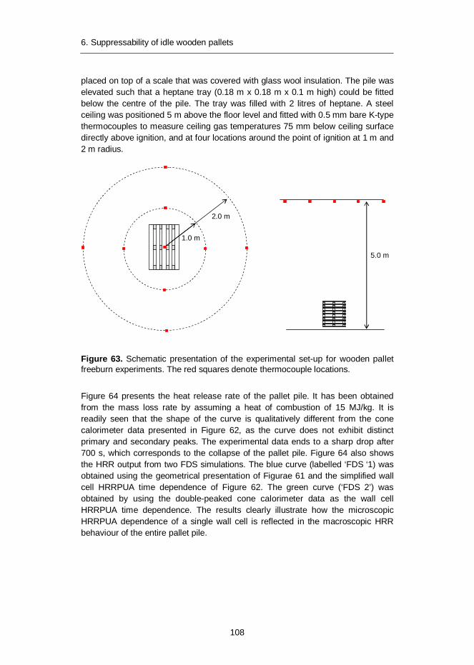
6. Suppressability of idle wooden pallets
108
placed on top of a scale that was covered with glass wool insulation. The pile was elevated such that a heptane tray (0.18 m x 0.18 m x 0.1 m high) could be fitted below the centre of the pile. The tray was filled with 2 litres of heptane. A steel ceiling was positioned 5 m above the floor level and fitted with 0.5 mm bare K-type thermocouples to measure ceiling gas temperatures 75 mm below ceiling surface directly above ignition, and at four locations around the point of ignition at 1 m and 2 m radius.
1.0 m
2.0 m
5.0 m
Figure 63. Schematic presentation of the experimental set-up for wooden pallet freeburn experiments. The red squares denote thermocouple locations.
Figure 64 presents the heat release rate of the pallet pile. It has been obtained from the mass loss rate by assuming a heat of combustion of 15 MJ/kg. It is readily seen that the shape of the curve is qualitatively different from the cone calorimeter data presented in Figure 62, as the curve does not exhibit distinct primary and secondary peaks. The experimental data ends to a sharp drop after 700 s, which corresponds to the collapse of the pallet pile. Figure 64 also shows the HRR output from two FDS simulations. The blue curve (labelled ‘FDS ‘1) was obtained using the geometrical presentation of Figurae 61 and the simplified wall cell HRRPUA time dependence of Figure 62. The green curve (‘FDS 2’) was obtained by using the double-peaked cone calorimeter data as the wall cell HRRPUA time dependence. The results clearly illustrate how the microscopic HRRPUA dependence of a single wall cell is reflected in the macroscopic HRR behaviour of the entire pallet pile.
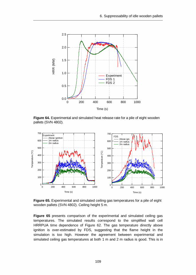
6. Suppressability of idle wooden pallets
109
Figure 64. Experimental and simulated heat release rate for a pile of eight wooden pallets (SVN 4802).
Figure 65. Experimental and simulated ceiling gas temperatures for a pile of eight wooden pallets (SVN 4802). Ceiling height 5 m.
Figure 65 presents comparison of the experimental and simulated ceiling gas temperatures. The simulated results correspond to the simplified wall cell HRRPUA time dependence of Figure 62. The gas temperature directly above ignition is over-estimated by FDS, suggesting that the flame height in the simulation is too high. However the agreement between experimental and simulated ceiling gas temperatures at both 1 m and 2 m radius is good. This is in
2.5
2.0
1.5
1.0
0.5
0.0
HR
R (M
W)
10008006004002000
Time (s)
Experiment FDS 1 FDS 2
700
600
500
400
300
200
100
0
Tem
pera
ture
(°C
)
10008006004002000
Time (s)
Experiment Above ignition 1m radius 2m radius
700
600
500
400
300
200
100
0
Tem
pera
ture
(°C
)
10008006004002000
Time (s)
FDS Above ign. 1m radius 2m radius
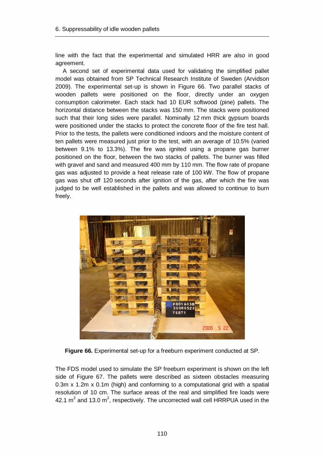
6. Suppressability of idle wooden pallets
110
line with the fact that the experimental and simulated HRR are also in good agreement.
A second set of experimental data used for validating the simplified pallet model was obtained from SP Technical Research Institute of Sweden (Arvidson 2009). The experimental set-up is shown in Figure 66. Two parallel stacks of wooden pallets were positioned on the floor, directly under an oxygen consumption calorimeter. Each stack had 10 EUR softwood (pine) pallets. The horizontal distance between the stacks was 150 mm. The stacks were positioned such that their long sides were parallel. Nominally 12 mm thick gypsum boards were positioned under the stacks to protect the concrete floor of the fire test hall. Prior to the tests, the pallets were conditioned indoors and the moisture content of ten pallets were measured just prior to the test, with an average of 10.5% (varied between 9.1% to 13.3%). The fire was ignited using a propane gas burner positioned on the floor, between the two stacks of pallets. The burner was filled with gravel and sand and measured 400 mm by 110 mm. The flow rate of propane gas was adjusted to provide a heat release rate of 100 kW. The flow of propane gas was shut off 120 seconds after ignition of the gas, after which the fire was judged to be well established in the pallets and was allowed to continue to burn freely.
Figure 66. Experimental set-up for a freeburn experiment conducted at SP.
The FDS model used to simulate the SP freeburn experiment is shown on the left side of Figure 67. The pallets were described as sixteen obstacles measuring 0.3m x 1.2m x 0.1m (high) and conforming to a computational grid with a spatial resolution of 10 cm. The surface areas of the real and simplified fire loads were 42.1 m2 and 13.0 m2, respectively. The uncorrected wall cell HRRPUA used in the
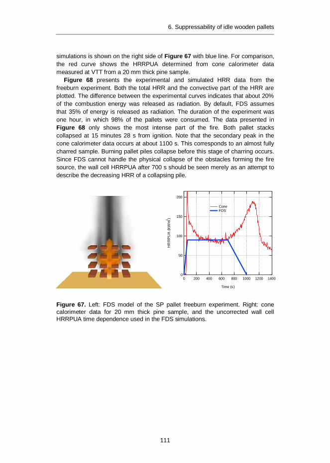
6. Suppressability of idle wooden pallets
111
simulations is shown on the right side of Figure 67 with blue line. For comparison, the red curve shows the HRRPUA determined from cone calorimeter data measured at VTT from a 20 mm thick pine sample.
Figure 68 presents the experimental and simulated HRR data from the freeburn experiment. Both the total HRR and the convective part of the HRR are plotted. The difference between the experimental curves indicates that about 20% of the combustion energy was released as radiation. By default, FDS assumes that 35% of energy is released as radiation. The duration of the experiment was one hour, in which 98% of the pallets were consumed. The data presented in Figure 68 only shows the most intense part of the fire. Both pallet stacks collapsed at 15 minutes 28 s from ignition. Note that the secondary peak in the cone calorimeter data occurs at about 1100 s. This corresponds to an almost fully charred sample. Burning pallet piles collapse before this stage of charring occurs. Since FDS cannot handle the physical collapse of the obstacles forming the fire source, the wall cell HRRPUA after 700 s should be seen merely as an attempt to describe the decreasing HRR of a collapsing pile.
Figure 67. Left: FDS model of the SP pallet freeburn experiment. Right: cone calorimeter data for 20 mm thick pine sample, and the uncorrected wall cell HRRPUA time dependence used in the FDS simulations.
200
150
100
50
0
HR
RP
UA
(kW
/m2 )
1400120010008006004002000
Time (s)
Cone FDS

6. Suppressability of idle wooden pallets
112
Figure 68. Experimental and simulated HRR data for the SP wooden pallet free-burn experiment (SVN 5002).
6.3 Water suppression
For the solid phase, water reduces the fuel pyrolysis rate primarily by cooling the surface. If the burning of the solid surface has been described using reaction parameters, there is no need to set additional suppression parameters. However, if the surface has been assigned a HRRPUA, there is a need for an empirical parameter that governs the behaviour of HRRPUA due to water application on the surface.
The suppression parameter (E_COEFFICIENT on the SURF-line of the FDS input file, here denoted simply as k) used by FDS is based on the work by Yu et al. (1994) on suppression of rack-storage fires by water. In that work it was found that the global heat release rate for a commodity depends on the mass application rate per unit area of water on top of the commodity in the form
(32)
with
(33)
4000
3000
2000
1000
0
HR
R (k
W)
120010008006004002000
Time (s)
Total HRR (experiment) Convective HRR (experiment) Total HRR (FDS) Convective HRR (FDS)
00
ttkeQQ
bmak
6. Suppressability of idle wooden pallets
113
where a (in units of m2/kg/s) and b (1/s) are to be determined experimentally. Subsequent work by Hamins, McGrattan and Forney (Hamins & McGrattan 1999, McGrattan et al. 2000, Hamins & McGrattan 2002) essentially supported the model. However, out of ’code development’ reasons the mass application rate was replaced by the concept of ’water application’, defined as
(34)
where A is the area of the top face of the commodity, U is the vertical velocity of droplets cascading down the sides of the commodity (0.54 m/s) and P is the perimeter of the commodity. Accordingly, the definition of parameter k takes the form
(35)
where a (in units of 1/s) is obtained from experiments. The local burning rate is obtained as
(36)
In the practical code implementation the effectiveness of water is evaluated through the array containing the water mass per unit area, WMPUA.
For evaluating the suppression parameter, experimental data from a commodity classification test series was used (Arvidson & Lönnermark 2002). The experimental set-up for wooden pallets is shown in Figure 69. The fire source consisted of 32 slatted wooden (pine) pallets measuring 1200 mm x 1000 mm x 150 mm (high) arranged in four piles in a 2 x 1 x 2 (high) configuration. The moisture content of the pallets was 10–12%. The pile was ignited by a heptane tray measuring 300 mm x 300 mm x 100 mm (high) filled with 1 litre of heptane on a 1 litre water base. A water applicator was fitted 300 mm above the top of the fire source that consisted of 24 full-cone, wide angle nozzles (4 x 6 square grid) with a 450 mm spacing. The fire source and water applicator were located under an oxygen consumption calorimeter. The water applicator was started when the convective heat release rate was 2 MW. Tests were conducted for water application densities of 5.0 mm/min, 7.5 mm/min, and 10.0 mm/min.
PUAmm
tmatk
dttkff etmtm 0,

6. Suppressability of idle wooden pallets
114
Figure 69. Commodity classification test for idle wooden pallets.
The FDS model of the pallet suppression tests is shown on left side of Figure 70. The pallets are described as 36 obstacles measuring 0.2 m x 1.2 m x 0.1 m (high) and conforming to a computational grid with a spatial resolution of 10 cm. The surface areas of the real and simplified fire loads are 96.2 m2 and 27.3 m2, respectively. The uncorrected wall cell HRRPUA used in the simulations is shown on right side of Figure 70. For comparison, the red curve shows the HRRPUA determined from cone calorimeter data measured at VTT from a 20 mm thick pine sample. In comparison to Figure 67, the HRRPUA used for FDS has a higher value (120 kW/m2) and a longer duration. The higher value was found necessary to reproduce the fire growth rate up to a convective HRR of 2MW. The longer duration was specified to ensure that the fuel would not run out due to the longer duration of a suppression test compared to a freeburn test.
The water nozzles were specified as Lechler 460.408 (5 mm/min), Lechler 460.448 (7.5 mm/min), and Lechler 460.528 (10 mm/min). The nozzles were operated at 2 bar, 3 bar, and 2 bar, respectively. All nozzles had a spray angle of 120 degrees. A median volume diameter of 400 m was assumed for densities 5 mm/min and 7.5 mm/min, and a median volume diameter of 500 m was assumed for the density 10 mm/min. No information on the drop sizes could be found in the Lechler data sheets.
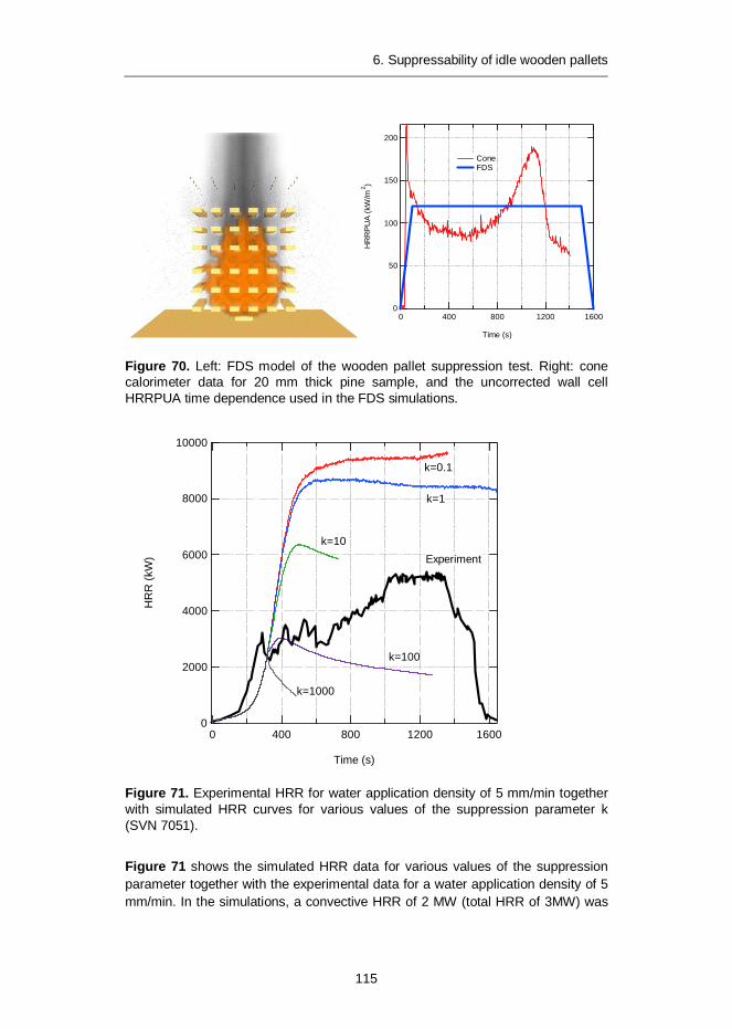
6. Suppressability of idle wooden pallets
115
Figure 70. Left: FDS model of the wooden pallet suppression test. Right: cone calorimeter data for 20 mm thick pine sample, and the uncorrected wall cell HRRPUA time dependence used in the FDS simulations.
Figure 71. Experimental HRR for water application density of 5 mm/min together with simulated HRR curves for various values of the suppression parameter k (SVN 7051).
Figure 71 shows the simulated HRR data for various values of the suppression parameter together with the experimental data for a water application density of 5 mm/min. In the simulations, a convective HRR of 2 MW (total HRR of 3MW) was
200
150
100
50
0
HR
RPU
A (k
W/m
2 )
160012008004000
Time (s)
Cone FDS
10000
8000
6000
4000
2000
0
HR
R (k
W)
160012008004000
Time (s)
Experiment
k=0.1
k=1
k=10
k=100
k=1000
6. Suppressability of idle wooden pallets
116
achieved at 320 s from ignition, at which point the water applicator was activated. It is observed that the onset of water application resulted in a sharp initial decrease in the experimental HRR, followed by a gradual increase up to a peak value of about 5 MW. For all values of the suppression parameter, the qualitative shape of the simulated HRR curve differs from the experimental result. Values of 10 or less are too small, resulting in too little suppression. A value of 100 provides a good HRR prediction at early stages of suppression, but it shows no initial decrease in the HRR, and no gradual increase at later stages. A value of 1000 provides a sharp initial decrease, but in accordance with the mathematical formulation of the model, the decrease is monotonous. The results of Figure 71 therefore raise a question of the validity of the current suppression parameter model for pallet piles.
As noted in the FDS Technical Reference Manual, the mathematical formulation for the suppression parameter model follows from a global energy balance for a complex fuel array. The derivation of the exponential decay of the HRR as a function of time assumes that the reduction of HRR is due to reduction in the surface area of the fuel undergoing pyrolysis (the surface is either burning or not burning) (Yu et al. 1994). However, FDS applies the exponential law locally, i.e. it assumes that the mass loss rate of a surface cell is exponentially dependent on the time a fixed water application rate hits the cell. This is locally awkward because the local water application rate may change as a function of time, for example because as the fire is suppressed, more water is able to penetrate to the seat of the fire.
There is experimental evidence (Magee & Reitz 1975) showing that below water application rates to achieve extinguishment, the steady-state mass loss rate per unit area of fuel exhibits a linear dependence on the water application rate per unit area. Furthermore, Magee and Reitz (1975) show that the linear dependence is entirely explained by the heat of evaporation of water. For PMMA, water reduces the burning rate of fuel such that the ratio of water mass application rate per fuel unit area to the fuel mass pyrolysis rate per fuel unit area is 6.5. On the other hand, Magee and Reitz (1975) also show that with water application rates above a critical rate to achieve extinguishment, the time to extinguishment is approximately an exponential function of time. It should be noted that many of the water application rates in Yu et al. (1994) were high enough to provide at least fire suppression.
In FDS, the surface cooling due to water is measured by the cooling effectiveness per unit area, WCPUA. This includes both heating of water up to the boiling point as well as evaporation of water. However, as evaporation requires significantly more energy per unit mass than heating, WCPUA essentially measures the evaporative cooling provided by water, unless the water application is large enough to reduce surface temperature of the fuel below the boiling point of water. For ordinary solid combustibles undergoing pyrolysis supporting combustion, this is never the case. An argument is therefore made that for fires defined by a prescriptive heat release rate, the suppression effectiveness of water
6. Suppressability of idle wooden pallets
117
is proportional to the instantaneous WCPUA. Thus, the mass flux of fuel due to water suppression, Wm , is computed as
(37)
Figure 72 presents the experimental and simulated HRR curves for wooden pallets for all three water application densities for the modified suppression parameter model. The simulated curves were computed with k=0.4 which resulted in the best qualitative overall agreement between experimental and simulated data. The simulated curves exhibit a correct qualitative shape, with an initial sharp decrease and a gradual increase of the HRR. The peak HRR value is slightly underestimated for 5 mm/min and overestimated for 10 mm/min. From visual inspection of the simulations, the initial decrease for HRR is due to the onset of cooling in the top part of the fuel array. The gradual increase is then due to the fire spreading in the lower part of the fuel array (5 mm/min and 7.5 mm/min). For 10 mm/min, there is enough water dripping through the array to the surfaces in lower parts to contain the fire in the centre of the array, preventing horizontal spread.
WW QkmMAXm 1,0 0

6. Suppressability of idle wooden pallets
118
Figure 72. Experimental and simulated HRR curves for wooden pallets with three different water application densities (SVN 5098).
6000
5000
4000
3000
2000
1000
0
HR
R (k
W)
150010005000
Time (s)
5 mm/min Experiment FDS
7.5 mm/min Experiment FDS
10 mm/min Experiment FDS
7. Road tunnels
119
7. Road tunnels Fires in road tunnels are rare events. When they happen, however, they can have catastrophic consequences both with respect to human life and material losses (vehicles, tunnel infrastructure). Recent examples of catastrophic road tunnel fires include the Mont Blanc tunnel (1999) with 39 deaths, Tauern tunnel (1999) with 12 deaths, and St. Gotthard tunnel (2001) with 11 deaths. In these fires, the cargo of a Heavy Goods Vehicle (HGV) played a key role.
It is estimated that the risk of road tunnel fires is gradually increasing due to growing density of traffic, growing number of tunnels and tunnel lengths, and vandalism (Haack 1994). Tunnel fires can be very intense. Modern vehicles may reach flashover conditions in a matter of few minutes. The limited vertical space in tunnels facilitates fire spread from one vehicle to another. The smoke from the fires may be pulled down by cold tunnel walls and recirculated back to the fire, reducing visibility and possibilities for safe escape. Fires involving multiple vehicles, if unsuppressed, may go on for hours if not days.
Because of the significant risk due to fires in tunnels, much effort has been put in understanding tunnel fires, their consequences, and importantly, ways to mitigate the consequences. The first European research effort to this effect was the EUREKA 499 project which involved eight European countries. This project provided the first systematic evidence for the extreme heat release rates (estimated to be above 100 MW) that were possible due to vehicle fires in tunnels, especially in the case of HGV fires and solid fire loads. Later, similar tests have been conducted in the Mont Blanc tunnel (Brousse et al. 2001), in the Second Benelux tunnel (Lemaire et al. 2002), and in Runehamar test tunnel (Ingason 2005), where the highest peak HRR values of about 200 MW for solid HGV fire loads were reported.
Due to the high cost of large-scale tunnel experiments, experimental research has also been carried out in model scale tunnels (Ingason 2008). Furthermore, there have been a few attempts to perform detailed CFD simulations on tunnel fire and fire suppression experiments (Cheong et al. 2009, Trelles & Mawhinney 2010). The particular purpose of the current work is to evaluate possibilities to predict rather than prescribe the performance of a tunnel fire suppression system by means of CFD.

7. Road tunnels
120
7.1 Runehamar tunnel
The fire tests conducted in Runehamar test tunnel, Norway, are reported in Lönnermark and Ingason (2005) and Ingason and Lönnermark (2005). Of the four tests conducted, this work considers Test 1 where the fire load consisted of wooden and plastic pallets. This test provides a well-documented case to evaluate the burning characteristics of the simplified FDS pallet model in a full-scale tunnel scenario.
7.1.1 FDS model of the tunnel
The Runehamar tunnel is a two-way-asphalted road tunnel 1600m long, 6m high and 9m wide, with a slope varying between 0.5% uphill and 1% downhill. The test fires were located 563 m from the tunnel downwind entrance. To protect the tunnel infrastructure, the tunnel walls were covered with fire protection boards over a distance of 75 m around the fire. Ventilation fans were located at the upwind entrance of the tunnel and they were capable of providing an air flow of 3–4 m/s in the tunnel. This flow velocity was chosen to reduce backlayering of smoke and to facilitate HRR measurement at the downwind end of the tunnel using oxygen consumption calorimetry.
The tunnel was instrumented to measure gas temperatures from 100 m upstream of the fire to 458 m downstream where a measuring station was located. The station was instrumented for gas temperature, gas velocity, and gas con-centration measurements (O2, CO2, CO) to enable HRR determination. Temperatures and gas velocities were measured at five different elevations, and gas concentrations at three different elevations. The tunnel cross section was thus divided into five horizontal segments, and the total HRR of the fire was obtained as a sum over individual HRR calculations in the five segments.
Figure 73 shows the overall structure of the FDS model for the Runehamar tunnel experiments. The whole length of the tunnel was not included in the model, which was reduced to a length of 792 m. The center of the fire source was located at position 0 m. The upwind end of the tunnel was at –204 m, and the downwind end at +588 m. The rectangular cross-section of the tunnel measured 9 m in width and 6 m in height. A pressure boundary with a dynamic pressure of 9.0 Pa provided the air flow in the tunnel. The computational domain was divided into five grids. Grid no. 2 (from –12 m to +12 m) contained the fire source, and it was modeled at a spatial resolution of 10 cm. All other grids were modeled at 20 cm resolution. Each grid had 1.3 million cells. Neither the sloping nor the curvature of the tunnel was taken into account in the model.
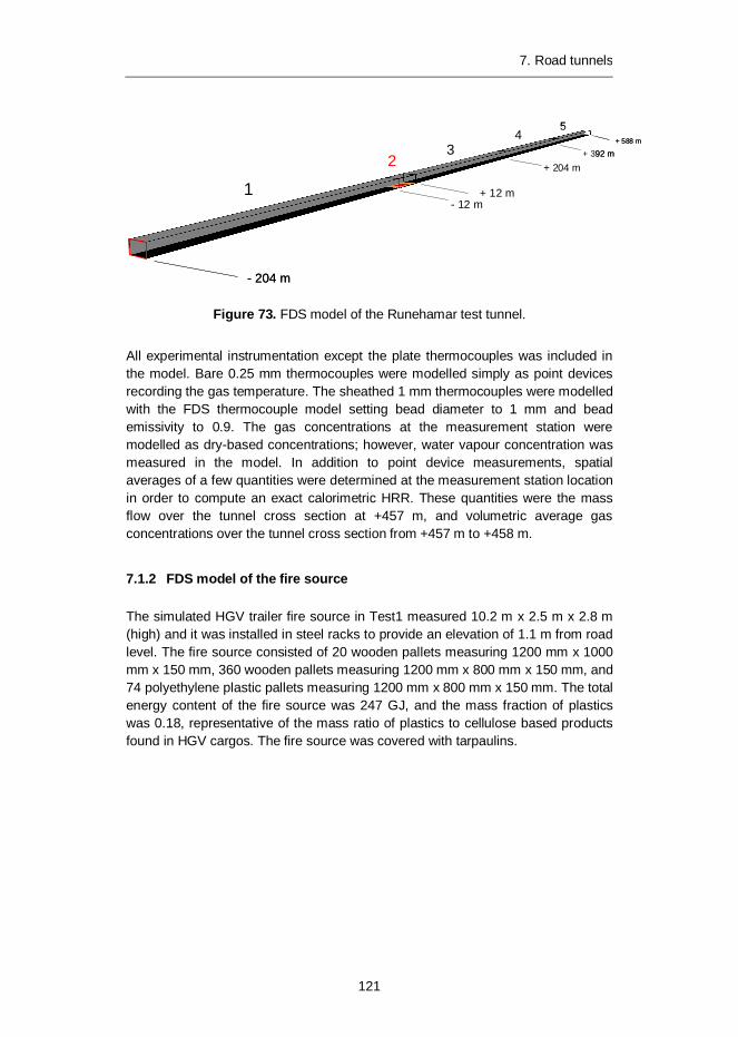
7. Road tunnels
121
Figure 73. FDS model of the Runehamar test tunnel.
All experimental instrumentation except the plate thermocouples was included in the model. Bare 0.25 mm thermocouples were modelled simply as point devices recording the gas temperature. The sheathed 1 mm thermocouples were modelled with the FDS thermocouple model setting bead diameter to 1 mm and bead emissivity to 0.9. The gas concentrations at the measurement station were modelled as dry-based concentrations; however, water vapour concentration was measured in the model. In addition to point device measurements, spatial averages of a few quantities were determined at the measurement station location in order to compute an exact calorimetric HRR. These quantities were the mass flow over the tunnel cross section at +457 m, and volumetric average gas concentrations over the tunnel cross section from +457 m to +458 m.
7.1.2 FDS model of the fire source
The simulated HGV trailer fire source in Test1 measured 10.2 m x 2.5 m x 2.8 m (high) and it was installed in steel racks to provide an elevation of 1.1 m from road level. The fire source consisted of 20 wooden pallets measuring 1200 mm x 1000 mm x 150 mm, 360 wooden pallets measuring 1200 mm x 800 mm x 150 mm, and 74 polyethylene plastic pallets measuring 1200 mm x 800 mm x 150 mm. The total energy content of the fire source was 247 GJ, and the mass fraction of plastics was 0.18, representative of the mass ratio of plastics to cellulose based products found in HGV cargos. The fire source was covered with tarpaulins.
1
32
54
- 204 m
- 12 m+ 12 m
+ 204 m+ 392 m
+ 588 m
1
32
54
- 204 m
- 12 m+ 12 m
+ 204 m+ 392 m
+ 588 m

7. Road tunnels
122
Figure 74. FDS model of the Runehamar Test 1 fire source.
Figurae 74 shows the FDS model of the fire source with a photograph of the real fire source as an inset. In the FDS model of the fire source, the pallets were described as 216 obstacles measuring 0.2 m x 2.4 m x 0.1 m (high) and conforming to a computational grid with a spatial resolution of 10 cm. Of the 216 obstacles, 36 represented plastic material. The surface areas of the real and simplified fire loads were 898 m2 and 296 m2, respectively. The uncorrected wall cell HRRPUA used in the simulations for wood and plastics is shown in Figure 75. The data for plastics is taken from Hirschler (1992) corresponding to an incident flux of 40 kW/m2. The fire protection boards surrounding the fire source, and the 10 cm thick sand layer below the fire source protecting the asphalt were included in the model. The tarpaulins were not included in the model.
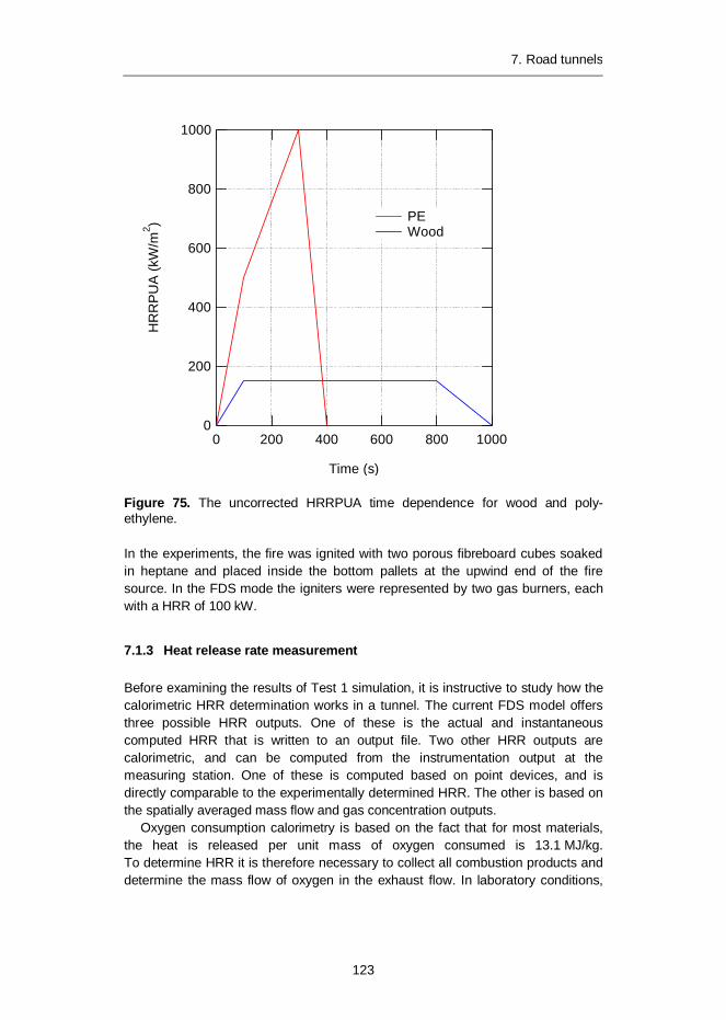
7. Road tunnels
123
Figure 75. The uncorrected HRRPUA time dependence for wood and poly-ethylene.
In the experiments, the fire was ignited with two porous fibreboard cubes soaked in heptane and placed inside the bottom pallets at the upwind end of the fire source. In the FDS mode the igniters were represented by two gas burners, each with a HRR of 100 kW.
7.1.3 Heat release rate measurement
Before examining the results of Test 1 simulation, it is instructive to study how the calorimetric HRR determination works in a tunnel. The current FDS model offers three possible HRR outputs. One of these is the actual and instantaneous computed HRR that is written to an output file. Two other HRR outputs are calorimetric, and can be computed from the instrumentation output at the measuring station. One of these is computed based on point devices, and is directly comparable to the experimentally determined HRR. The other is based on the spatially averaged mass flow and gas concentration outputs.
Oxygen consumption calorimetry is based on the fact that for most materials, the heat is released per unit mass of oxygen consumed is 13.1 MJ/kg. To determine HRR it is therefore necessary to collect all combustion products and determine the mass flow of oxygen in the exhaust flow. In laboratory conditions,
1000
800
600
400
200
0
HR
RP
UA
(kW
/m2 )
10008006004002000
Time (s)
PE Wood

7. Road tunnels
124
the exhaust gases flow in a duct under well-mixed conditions and therefore a single point measurement inside the duct gives sufficient accuracy. In tunnels however the downwind section is not generally well-mixed, but there is a distinct temperature, velocity, and oxygen concentration profile in the vertical direction (Ingason 1994). For obtaining accurate results, the tunnel cross section needs to be divided in segments, and the total HRR is obtained as a sum over the HRR values from each segment. This requires a fair amount of instrumentation.
When point devices are used in a segment of cross section A, the mass flow rate through the segment is obtained as
(38)
where the factor i is the ratio of the mean gas velocity to the maximum gas velocity in segment i. A value of 0.817 was used by Ingason and Lönnermark (2005). With measurements of the volumetric concentrations XO2 and XCO2 available, and neglecting CO, the heat release rate in segment i is obtained as
(39)
where E=13.1 MJ/kg, =1.105 (expansion factor), superscript 0 refers to incoming air, and subscript i has been omitted for clarity from the gas concentration measurements. In the Runehamar experiments, gas concentrations were measured only at two or three heights, and the ‘missing’ values were found by interpolation.
When spatially averaged quantities are used, and gas concentrations XO2, XCO2, XCO and XH2O are measured (oxygen, CO2 and CO still dry-based), the total mass flow is taken into account to within 99% (Janssens & Parker 1992). In this case, the heat release rate is obtained as
(40)
where ECO is the enthalpy per unit mass of oxygen for CO oxidation to CO2, 17.6 MJ/kg, and the oxygen depletion factor is
(41)
iii
ii AuT
Tm 00
20
220
2
220
2
022
111111
COCOOO
COO
O
OHAIROii
XXXXXX
X
XMMmEQ
02
02
2
2
12
1OOHAIR
AIR
O
O
COCOi XXm
MM
XXEEEQ
0002
02
022
002
02
111
COCOCOO
COOCOCOO
XXXXXXXXX
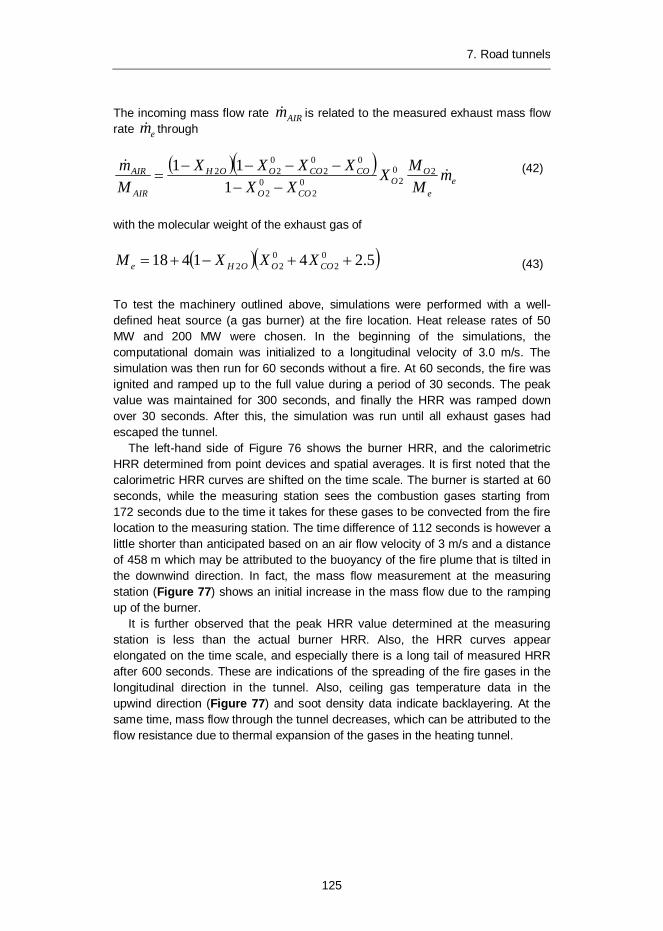
7. Road tunnels
125
The incoming mass flow rate AIRm is related to the measured exhaust mass flow rate em through
(42)
with the molecular weight of the exhaust gas of
(43)
To test the machinery outlined above, simulations were performed with a well-defined heat source (a gas burner) at the fire location. Heat release rates of 50 MW and 200 MW were chosen. In the beginning of the simulations, the computational domain was initialized to a longitudinal velocity of 3.0 m/s. The simulation was then run for 60 seconds without a fire. At 60 seconds, the fire was ignited and ramped up to the full value during a period of 30 seconds. The peak value was maintained for 300 seconds, and finally the HRR was ramped down over 30 seconds. After this, the simulation was run until all exhaust gases had escaped the tunnel.
The left-hand side of Figure 76 shows the burner HRR, and the calorimetric HRR determined from point devices and spatial averages. It is first noted that the calorimetric HRR curves are shifted on the time scale. The burner is started at 60 seconds, while the measuring station sees the combustion gases starting from 172 seconds due to the time it takes for these gases to be convected from the fire location to the measuring station. The time difference of 112 seconds is however a little shorter than anticipated based on an air flow velocity of 3 m/s and a distance of 458 m which may be attributed to the buoyancy of the fire plume that is tilted in the downwind direction. In fact, the mass flow measurement at the measuring station (Figure 77) shows an initial increase in the mass flow due to the ramping up of the burner.
It is further observed that the peak HRR value determined at the measuring station is less than the actual burner HRR. Also, the HRR curves appear elongated on the time scale, and especially there is a long tail of measured HRR after 600 seconds. These are indications of the spreading of the fire gases in the longitudinal direction in the tunnel. Also, ceiling gas temperature data in the upwind direction (Figure 77) and soot density data indicate backlayering. At the same time, mass flow through the tunnel decreases, which can be attributed to the flow resistance due to thermal expansion of the gases in the heating tunnel.
ee
OO
COO
COCOOOH
AIR
AIR mMMX
XXXXXX
Mm 20
202
02
002
022
111
5.241418 02
022 COOOHe XXXM
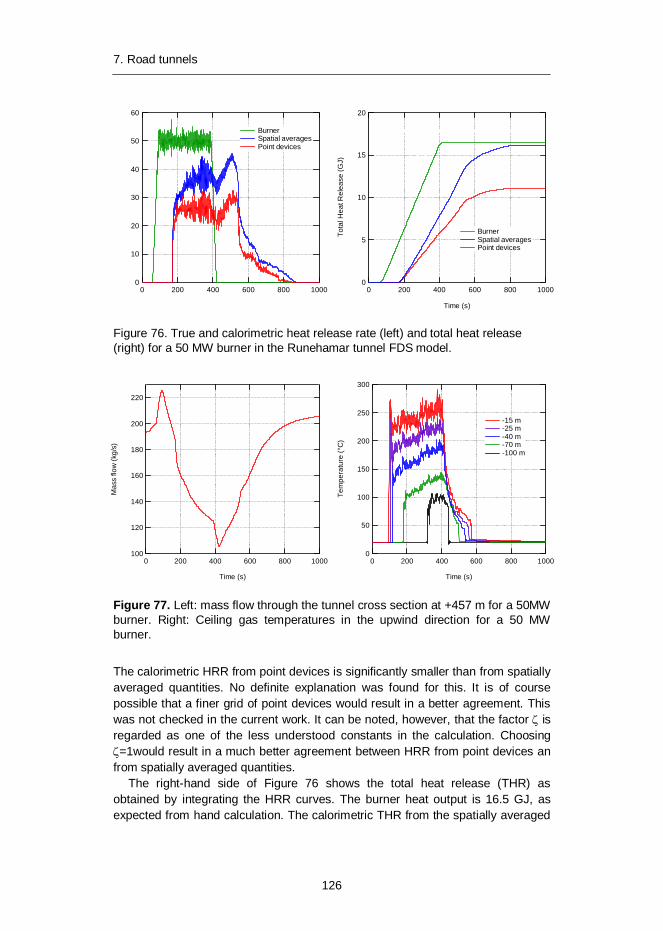
7. Road tunnels
126
Figure 76. True and calorimetric heat release rate (left) and total heat release (right) for a 50 MW burner in the Runehamar tunnel FDS model.
Figure 77. Left: mass flow through the tunnel cross section at +457 m for a 50MW burner. Right: Ceiling gas temperatures in the upwind direction for a 50 MW burner.
The calorimetric HRR from point devices is significantly smaller than from spatially averaged quantities. No definite explanation was found for this. It is of course possible that a finer grid of point devices would result in a better agreement. This was not checked in the current work. It can be noted, however, that the factor is regarded as one of the less understood constants in the calculation. Choosing =1would result in a much better agreement between HRR from point devices an
from spatially averaged quantities. The right-hand side of Figure 76 shows the total heat release (THR) as
obtained by integrating the HRR curves. The burner heat output is 16.5 GJ, as expected from hand calculation. The calorimetric THR from the spatially averaged
60
50
40
30
20
10
010008006004002000
Burner Spatial averages Point devices
20
15
10
5
0
Tota
l Hea
t Rel
ease
(GJ)
10008006004002000
Time (s)
Burner Spatial averages Point devices
220
200
180
160
140
120
100
Mas
s flo
w (k
g/s)
10008006004002000
Time (s)
300
250
200
150
100
50
0
Tem
pera
ture
(°C
)
10008006004002000
Time (s)
-15 m -25 m -40 m -70 m -100 m
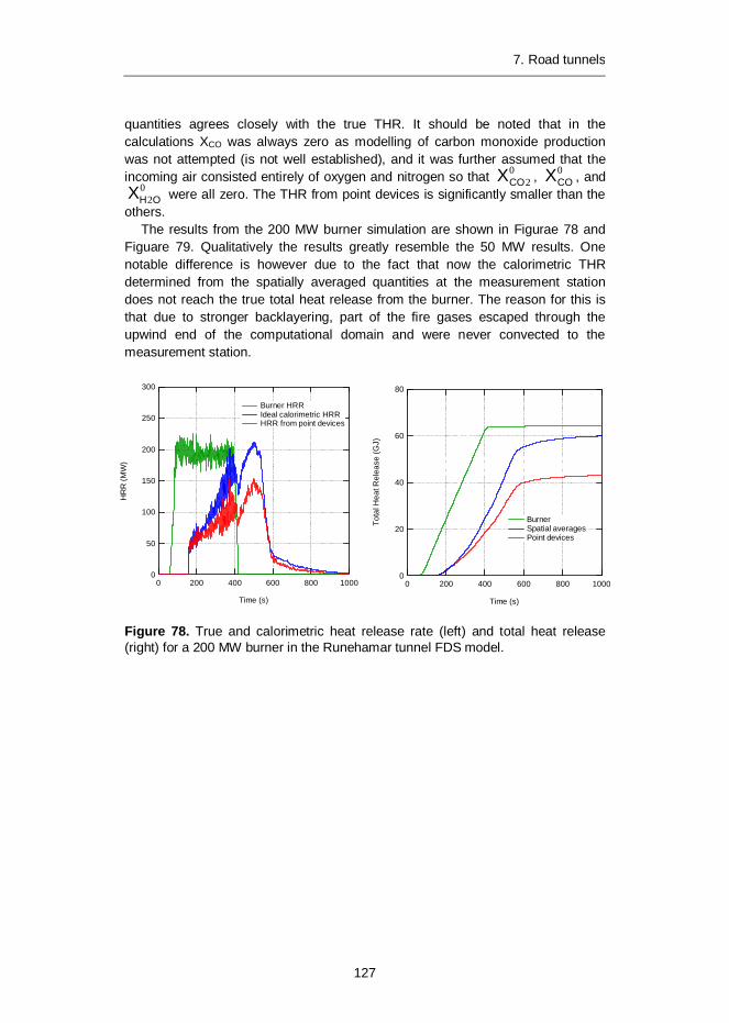
7. Road tunnels
127
quantities agrees closely with the true THR. It should be noted that in the calculations XCO was always zero as modelling of carbon monoxide production was not attempted (is not well established), and it was further assumed that the incoming air consisted entirely of oxygen and nitrogen so that 0
2COX , 0COX , and
02OHX were all zero. The THR from point devices is significantly smaller than the
others. The results from the 200 MW burner simulation are shown in Figurae 78 and
Figuare 79. Qualitatively the results greatly resemble the 50 MW results. One notable difference is however due to the fact that now the calorimetric THR determined from the spatially averaged quantities at the measurement station does not reach the true total heat release from the burner. The reason for this is that due to stronger backlayering, part of the fire gases escaped through the upwind end of the computational domain and were never convected to the measurement station.
Figure 78. True and calorimetric heat release rate (left) and total heat release (right) for a 200 MW burner in the Runehamar tunnel FDS model.
300
250
200
150
100
50
0
HR
R (M
W)
10008006004002000
Time (s)
Burner HRR Ideal calorimetric HRR HRR from point devices
80
60
40
20
0
Tota
l Hea
t Rel
ease
(GJ)
10008006004002000
Time (s)
Burner Spatial averages Point devices

7. Road tunnels
128
Figure 79. Left: mass flow through the tunnel cross section at +457 m for a 50MW burner. Right: Ceiling gas temperatures in the upwind direction for a 50 MW burner.
7.1.4 Test 1 heat release rate
Figure 80 presents the experimental and simulated heat release rate from Runehamar Test 1. The blue curve has been obtained with the tunnel model shown in Figure 65. The red curve has been obtained with a shorter model, from -60 m to +60 m. Both simulation results exhibit a faster rate of growth compared to the experimental data. It should be noted however that the FDS result is the actual FDS output whereas the experimental results is calorimetrically determined. It turned out difficult to obtain the calorimetric estimate from the numerical simulations in the long tunnel model. As seen from the HRR curve, the model goes unstable soon after the HRR reaches 200 MW, and in fact the simulation ended due to a numerical instability after 570 seconds of real time. The use of a short tunnel directly denies determination of the calorimetric HRR. However the model remains stable even with the HRR exceeding 200 MW. The peak value is about 220 MW, in quite good agreement with the experimental peak value of 202 MW. The numerical challenge posed by tunnel geometries (or in general geometries where a flow is passing through many grids in serial arrangement) is a known issue for FDS. Development work is ongoing to improve the performance of the pressure solver. Despite the numerical instabilities, the results shown in Figure 76 – Figure 79 indicate that the tunnel causes a difference between the actual and calorimetrically determined heat release rates, and especially affects the observed fire growth rate and possibly the peak HRR value.
250
200
150
100
Mas
s flo
w (k
g/s)
10008006004002000
Time (s)
600
500
400
300
200
100
0
Tem
pera
ture
(°C
)
10008006004002000
Time (s)
-15 m -25 m -40 m -70 m -100 m
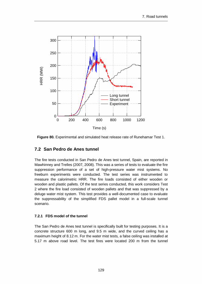
7. Road tunnels
129
Figure 80. Experimental and simulated heat release rate of Runehamar Test 1.
7.2 San Pedro de Anes tunnel
The fire tests conducted in San Pedro de Anes test tunnel, Spain, are reported in Mawhinney and Trelles (2007, 2008). This was a series of tests to evaluate the fire suppression performance of a set of high-pressure water mist systems. No freeburn experiments were conducted. The test series was instrumented to measure the calorimetric HRR. The fire loads consisted of either wooden or wooden and plastic pallets. Of the test series conducted, this work considers Test 2 where the fire load consisted of wooden pallets and that was suppressed by a deluge water mist system. This test provides a well-documented case to evaluate the suppressability of the simplified FDS pallet model in a full-scale tunnel scenario.
7.2.1 FDS model of the tunnel
The San Pedro de Anes test tunnel is specifically built for testing purposes. It is a concrete structure 600 m long, and 9.5 m wide, and the curved ceiling has a maximum height of 8.12 m. For the water mist tests, a false ceiling was installed at 5.17 m above road level. The test fires were located 200 m from the tunnel
300
250
200
150
100
50
0
HR
R (M
W)
120010008006004002000
Time (s)
Long tunnel Short tunnel Experiment
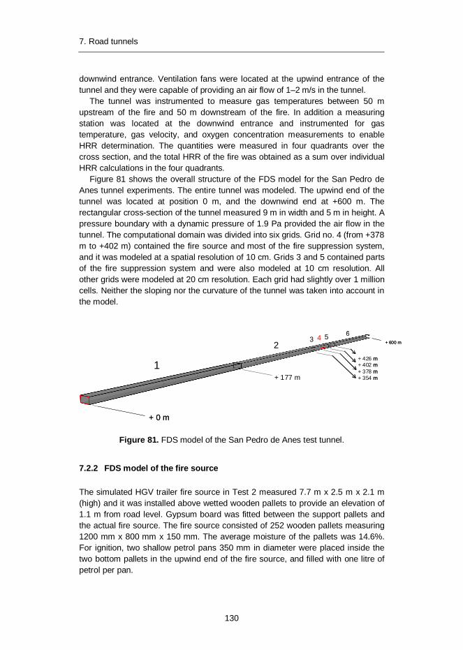
7. Road tunnels
130
downwind entrance. Ventilation fans were located at the upwind entrance of the tunnel and they were capable of providing an air flow of 1–2 m/s in the tunnel.
The tunnel was instrumented to measure gas temperatures between 50 m upstream of the fire and 50 m downstream of the fire. In addition a measuring station was located at the downwind entrance and instrumented for gas temperature, gas velocity, and oxygen concentration measurements to enable HRR determination. The quantities were measured in four quadrants over the cross section, and the total HRR of the fire was obtained as a sum over individual HRR calculations in the four quadrants.
Figure 81 shows the overall structure of the FDS model for the San Pedro de Anes tunnel experiments. The entire tunnel was modeled. The upwind end of the tunnel was located at position 0 m, and the downwind end at +600 m. The rectangular cross-section of the tunnel measured 9 m in width and 5 m in height. A pressure boundary with a dynamic pressure of 1.9 Pa provided the air flow in the tunnel. The computational domain was divided into six grids. Grid no. 4 (from +378 m to +402 m) contained the fire source and most of the fire suppression system, and it was modeled at a spatial resolution of 10 cm. Grids 3 and 5 contained parts of the fire suppression system and were also modeled at 10 cm resolution. All other grids were modeled at 20 cm resolution. Each grid had slightly over 1 million cells. Neither the sloping nor the curvature of the tunnel was taken into account in the model.
Figure 81. FDS model of the San Pedro de Anes test tunnel.
7.2.2 FDS model of the fire source
The simulated HGV trailer fire source in Test 2 measured 7.7 m x 2.5 m x 2.1 m (high) and it was installed above wetted wooden pallets to provide an elevation of 1.1 m from road level. Gypsum board was fitted between the support pallets and the actual fire source. The fire source consisted of 252 wooden pallets measuring 1200 mm x 800 mm x 150 mm. The average moisture of the pallets was 14.6%. For ignition, two shallow petrol pans 350 mm in diameter were placed inside the two bottom pallets in the upwind end of the fire source, and filled with one litre of petrol per pan.
+ 0 m
1
32
64 5
+ 177 m
+ 426 m+ 402 m+ 378 m+ 354 m
+ 600 m
+ 0 m
1
32
64 5
+ 177 m
+ 426 m+ 402 m+ 378 m+ 354 m
+ 600 m

7. Road tunnels
131
Figure 82 shows the FDS model of the fire source together with a photograph of the real fire source. In the FDS model of the fire source, the pallets were described as 102 obstacles measuring 0.2 m x 2.4 m x 0.1 m (high) and conforming to a computational grid with a spatial resolution of 10 cm. The surface areas of the real and simplified fire loads were 522 m2 and 151 m2, respectively. The uncorrected wall cell HRRPUA was ramped up linearly from 0 to 150 kW/m2 in a time of 100 seconds, after which it was kept constant. To model fuel burn-out, it was first noted that the obstacles occupy a volume of 4.896 m3. The real fire source weighs 6023 kg (23.9 kg per pallet), of which 5143.6 kg is dry mass. Each fuel obstacle was thus assigned a bulk density of 1050.6 kg/m3, which is one possibility to instruct FDS to account for fuel burn-out. In addition it was specified that FDS shall remove each fuel containing obstacle from the calculation once burn-out has occurred in that cell. The ignition sources were modelled as two 100 kW burners that were turned off after 5 minutes from ignition.
Figure 82. FDS model and photograph of the San Pedro de Anes Test 2 fire source. The yellow obstacles in the FDS model are the ignition burners.
7.2.3 FDS model of the high pressure water mist system
The nozzle layout for the high pressure water mist suppression system is shown in Figure 83. The deluge water mist system used in the simulations was set up according to the experimental arrangement used by Marioff Corporation Oy in the San Pedro de Anes test tunnel. A total of 24 nozzles were installed between +372 m and +400 m in three lines, each nozzle protecting an area of about 12 m2. The nozzle spacing within the lines was 4.0 m, and the spacing between the lines was 3.0 m. The discharge density was 3.8 mm/min and the total flow rate was 1180 l/min. The FDS default drop size distribution was used with median volume diameter of 150 m. The initial velocity of the droplets was 120 m/s. The spray pattern for each nozzle was constructed according to the HI-FOG 4S 1MD 6MD 1000 spray head multiport configuration. Each spray was modeled as a 15 degree wide full cone.
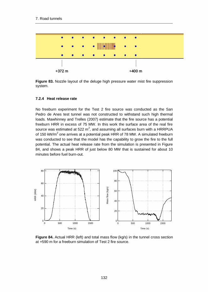
7. Road tunnels
132
Figure 83. Nozzle layout of the deluge high pressure water mist fire suppression system.
7.2.4 Heat release rate
No freeburn experiment for the Test 2 fire source was conducted as the San Pedro de Anes test tunnel was not constructed to withstand such high thermal loads. Mawhinney and Trelles (2007) estimate that the fire source has a potential freeburn HRR in excess of 75 MW. In this work the surface area of the real fire source was estimated at 522 m2, and assuming all surfaces burn with a HRRPUA of 150 kW/m2 one arrives at a potential peak HRR of 78 MW. A simulated freeburn was conducted to see that the model has the capability to grow the fire to the full potential. The actual heat release rate from the simulation is presented in Figure 84, and shows a peak HRR of just below 80 MW that is sustained for about 10 minutes before fuel burn-out.
Figure 84. Actual HRR (left) and total mass flow (kg/s) in the tunnel cross section at +590 m for a freeburn simulation of Test 2 fire source.
+372 m +400 m+372 m +400 m
80
60
40
20
0
HR
R (M
W)
150010005000
Time (s)
100
80
60
40
20
0
Mas
s flo
w (k
g/s)
150010005000
Time (s)

7. Road tunnels
133
The simulation also included instrumentation to determine the calorimetric HRR, but the air flow velocity of 2 m/s was not sufficient to prevent significant backlayering and escape of fire gases out ot the upwind end of the computational domain. This is reflected in the total mass flow rate determined for the tunnel cross section at +590 m (Figure 84, right). The initial mass flow rate is consistent with 2 m/s air flow, but once the fire delops, there is clear stratification along the entire length of the tunnel. In the downwind end this is observed as flow velocities of up to +4 m/s in the upper part of the tunnel, but in the lower part the air flow is towards the fire at about –2 m/s, resulting in a significantly reduced total mass flow.
Figure 85 shows the experimental and simulated HRR curves for deluge water mist system for Test 2. The experimental calorimetric HRR has been corrected for the estimated time delay between fire source and measurement station. The time from ignition to water mist system activation was 5 min 40 s. In this time the calorimetric HRR increased to about 10 MW. After activation, the experimental HRR developed slowly over 15 minutes to a peak value of about 23 MW, indicating a clear reduction in the HRR compared to the potential peak HRR.
Figure 85. Experimental and simulated HRR of a simulated HGV trailer fire suppressed with a deluge high pressure water mist system.
35
30
25
20
15
10
5
0
HR
R (M
W)
2000150010005000
Time (s)
Actual Calorimetric Experiment
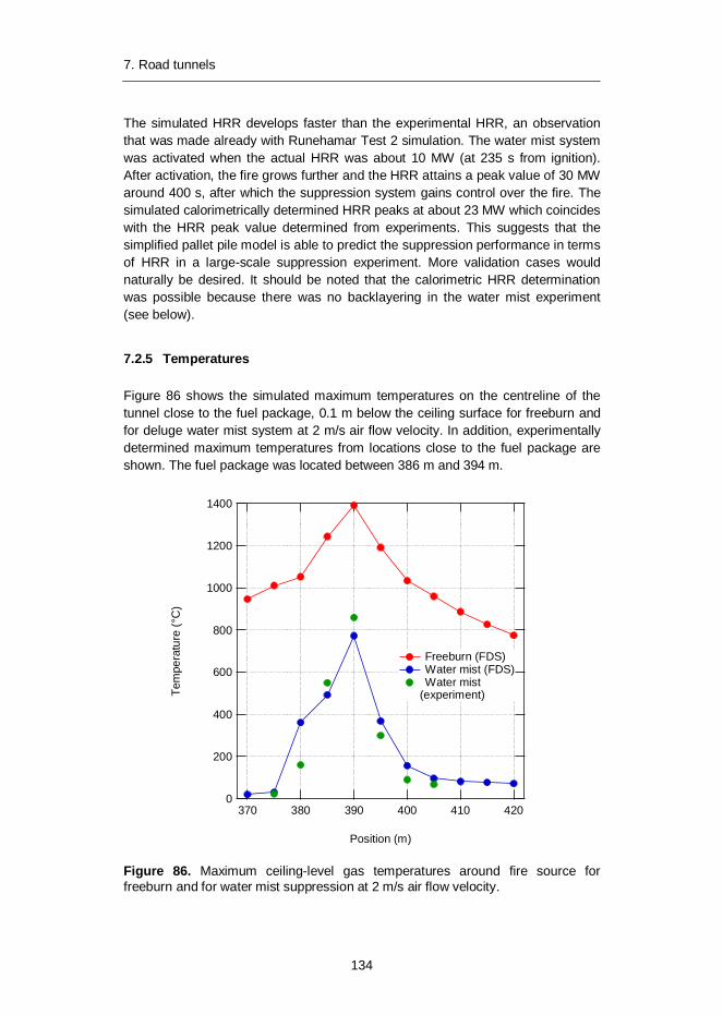
7. Road tunnels
134
The simulated HRR develops faster than the experimental HRR, an observation that was made already with Runehamar Test 2 simulation. The water mist system was activated when the actual HRR was about 10 MW (at 235 s from ignition). After activation, the fire grows further and the HRR attains a peak value of 30 MW around 400 s, after which the suppression system gains control over the fire. The simulated calorimetrically determined HRR peaks at about 23 MW which coincides with the HRR peak value determined from experiments. This suggests that the simplified pallet pile model is able to predict the suppression performance in terms of HRR in a large-scale suppression experiment. More validation cases would naturally be desired. It should be noted that the calorimetric HRR determination was possible because there was no backlayering in the water mist experiment (see below).
7.2.5 Temperatures
Figure 86 shows the simulated maximum temperatures on the centreline of the tunnel close to the fuel package, 0.1 m below the ceiling surface for freeburn and for deluge water mist system at 2 m/s air flow velocity. In addition, experimentally determined maximum temperatures from locations close to the fuel package are shown. The fuel package was located between 386 m and 394 m.
Figure 86. Maximum ceiling-level gas temperatures around fire source for freeburn and for water mist suppression at 2 m/s air flow velocity.
1400
1200
1000
800
600
400
200
0
Tem
pera
ture
(°C
)
420410400390380370
Position (m)
Freeburn (FDS) Water mist (FDS) Water mist
(experiment)

7. Road tunnels
135
In all cases, the maximum temperatures are observed directly above the centre of the fuel package. For freeburn, the maximum temperature of almost 1400 C is very high, and it is most likely too high given that temperatures in the 1300 1400 C range have been experimentally observed mostly in conjunction with fires involving combustible liquids (Ingason 2006). However, in Runehamar Test 1 (Lönnermark & Ingason 2005), gas temperatures above 1300 C were observed for a solid fire load. A possible explanation for the overestimation is that the model did not properly account for the cooling of the fuel surface due to evaporation of pyrolysis products, an effect known to lead to excessive fuel surface temperatures.
Despite the overestimation of the gas temperatures in the freeburn case, the results clearly demonstrate the reduction of gas temperatures due to a high pressure water mist fire suppression system, which is due to both reduction of the HRR, and evaporative cooling of the gas phase. For the water msit case, the gas temperatures close to the upwind end of the fuel package are reduced to the ambient temperature. This is due to the removal of backlayering caused by the water mist system (see below). The reduction of the maximum temperatures due to a water-based fire suppression system may affect the structural fire resistance requirements for the tunnel construction.
7.2.6 Backlayering
Backlayering means the spread of heat and smoke to both downwind and upwind directions from the fire source. This has implications with respect to both evacuation and manual fire fighting and rescue operations. Although the backlayering can be prevented by applying a sufficiently high air flow velocity in the tunnel, both experimental results and the simulation results of this study suggest that the fire suppression system may also affect backlayering. This was also observed experimentally.
Figure 87displays two snapshots of the soot distribution for 2 m/s air flow velocity. Notice that the pictures have been scaled in the longitudinal direction by a factor of 0.1 such that the entire 600 m long tunnel can be better visualized. The top picture shows the situation at 235 s, i.e. the moment when the suppression systems were activated. At that point, the smoke has already moved about 50 m in the upwind direction. The bottom picture shows the situation 100 seconds after the activation of the water mist system. All smoke is found either at fire location or in the downwind side of the fuel package, such that the water mist system has entirely prevented the backlayering of smoke. This is in accordance with the ceiling gas temperature data shown above.
A possible explanation for the ability of the high pressure water mist to prevent backlayering is connected to the kinetic energy of the water sprays which is able to overcome the buoyancy of the fire plume. On the other hand, buoyancy is also reduced due to the cooling capability of the water mist system.

7. Road tunnels
136
Figure 87. Spreading of smoke for air flow velocity of 2 m/s. Above: moment of suppression system activation. Below: 100 s after water mist system activation.

8. Summary
137
8. Summary This publication presents the main findings from a three-year research project with a goal to improve and enhance the capabilities of the NIST Fire Dynamics Simulator to describe water spray dynamics, discharge of large water based fire suppression systems, flame extinguishment, and the suppression of large complex solid fire loads. Significant emphasis was put on validation work against experimental data. When such data was not readily found in the literature, experiments were conducted to create the data.
In order to investigate the capability of FDS to simulate the dynamics of water mist sprays, three high pressure water mist micro nozzles and one low pressure fine water spray nozzle were experimentally characterized by the Direct Imaging (Shadowgraphy) technique to obtain the radial distributions of mean droplet size, mean droplet velocity, droplet mass flux, and droplet number concentration at an axial distance from the nozzle that corresponded to completion of the atomization process. Gross cumulative drop size distributions were constructed from the data that were given as the input for FDS together with the known water flow rate and initial drop velocity that was estimated from the water pressure. Spray angle was estimated from photographs. Comparisons of measured and simulated radial distributions showed relatively good agreement considering the simplistic de-scription of the droplet initial conditions in the simulations. Measurements were also performed to quantify the ability of the water sprays to entrain air by installing micro nozzles and spray heads consisting of several micro nozzles to rectangular channels and recording the air velocity behind the sprays. Simulations of the spray heads were done by superposing at the same point micro nozzles with different orientations. The deviation between experimental and simulated air velocities was not more than 20%. During the simulation process, the importance of the appropriate description of the momentum transfer between droplets and gas became obvious.
The ability of FDS to predict the activation of standard sprinklers and water mist sprinklers was studied for a set of experiments conducted under a 10 m x 20 m ceiling at 2.5 m or 4 m height and with a 1.7 MW heptane pool as the fire source. Both standard spray sprinklers (special response, 68°C) and water mist sprinklers (fast response, 57°C) were used. Up to 12 standard spray sprinklers were activated at 2.5 m height, while only up to 4 water mist sprinklers were activated. FDS simulations of the experiments suggested that FDS is able to predict the
8. Summary
138
number of activations for both standard spray and water mist sprinklers. Simulations were then carried out for both sprinkler types with a reduced spacing to see how spacing correlates to the number of activations. A very weak correlation was observed.
The ability of standard spray sprinklers to cool a fire plume was computationally evaluated for heat release rates between 5–20 MW and a ceiling height of 10 m. Discharge densities between 12.5 mm/min and 43 mm/min were investigated, the latter corresponding to an ESFR sprinkler system. The ESFR system was found to provide effective gas-phase cooling up to 20 MW, by reducing gas temperatures to around 200°C, a temperature that requires no passive protection measures for exposed steel structures. The results for lower discharge densities showed a very high sensitivity to the choice of the droplet size spectrum, underlining the need for drop size data when performing computational estimations of the gas-phase cooling ability.
An improved flame extinguishing criterion was implemented to FDS for gaseous suppressants under the lumped species model with transport-limited combustion (infinitely fast chemistry). The criterion considers the total enthalpy of gas mixture as a function of temperature, and evaluates whether a limiting adiabatic flame temperature can be obtained due to combustion in a cell. The model was validated against a number of experiments in the cup burner apparatus, a standard means of obtaining the minimum flame-extinguishing concentrations (MEC) for a variety of fuel-suppressant combinations. The results indicated that the model could reproduce the MEC values for all common inert gas agents, as well as some of the fluorinated halocarbon agents. It was further demonstrated that the flame extinguishment criterion, although validated using grid cells on the order of 1 mm, is equally applicable to larger cell sizes more appropriate for full-scale simulations. This improves the capability of FDS to predict the performance of full-scale fire suppression systems.
Piles of idle wooden pallets are often found in industrial or warehouse environments, and they form a significant fire hazard especially when they are located inside buildings or close to exterior walls of buildings. As pallets are standardized, cheap and readily available in large quantities, they are an attractive choice as a solid fire load in many large-scale fire suppression experiments, and especially in simulated vehicle fires. For simulations of large-scale fire tests where piles of idle wooden pallets are used as the fire source, spatial resolutions are required that are not capable of capturing the true geometry of the fire source. A simplified model for pallet piles was constructed for a 10 cm spatial resolution whose burning properties and suppressability by water was evaluated against experimental data.
Fires in road tunnels are rare events. When they happen, however, they can have catastrophic consequences both with respect to human life and material losses (vehicles, tunnel infrastructure). Because of the significant risk due to fires in tunnels, much effort has been put in understanding tunnel fires, their consequences, and importantly, ways to mitigate the consequences. Due to the high cost of large-scale tunnel experiments, experimental research has been

8. Summary
139
carried out in model scale tunnels, and there have been a few attempts to perform detailed CFD simulations on tunnel fire and fire suppression experiments; however these simulations focussed on the thermal management provided by the water based suppression system. In this project, possibilities were evaluated to predict rather than prescribe the performance of a tunnel fire suppression system by means of CFD. The simplified pallet burning model was used to simulate a large freeburn tunnel experiment and a large fire suppression experiment with a qualitative agreement between experiment and simulations

140
References
Arvidson, M. and Lönnermark, A. 2002. Commodity Classification Tests of Selected Ordinary Combustible Products. SP Report 2002:03. SP Swedish National Testing and Research Institute, Borås.
Arvidson, M. and Hertzberg, T. 2003. The VINNOVA water mist research project: a description of the 500 m3 machinery space tests. SP Report 2003:19. SP Swedish National Testing and Research Institute, Borås.
Arvidson, M. 2009. Private communication. SP Technical Research Institute of Sweden, Borås.
Back, G., Beyler, C., DiNenno, P. and Hansen, R. 2000. Water Mist Fire Protection for Very Large Machinery Spaces. USCG Report No CG-D-15-00. U.S. Coast Guard R&D Centre, Groton, CT.
Beyler, C. L. 2002. Flammability Limits of Premixed and Diffusion Flames. In: The SFPE Handbook of Fire Protection Engineering (3rd ed), DiNenno P.J. (ed.). National Fire Protection Association, Quincy, MA. P. 2/173.
Brousse, B., Perard, M., Voeltzel, A. and Botlan, Y. L. 2001. Ventilation and fire tests in the Mont Blanc Tunnel to better understand the catastrophic fire of March 24th, 1999. In: Third international conference on tunnel fires and escape from tunnels, Washington DC, USA. Pp. 211–222.
Burcat, A. and Ruscic, B. 2005. Third Millennium Ideal Gas and Condensed Phase Thermochemical Database for Combustion with Updates from Active Thermochemical Tables. ANL-05/20. Argonne National Laboratory, Argonne.
Chan, S. C., Bryant, J. T., Spicer, L. D. and Rabinovitch, B. S. 1970. Relative Cross Sections of Fluoroalkanes and Nitriles. Journal of Physical Chemistry, Vol. 74, pp. 2058–2064.
Cheong, M. K., Spearpoint, M. J. and Fleischmann, C. M. 2009. Calibrating an FDS Simulation of Goods-vehicle Fire Growth in a Tunnel Using the Runehamar Experiment. Journal of Fire Protection Engineering, Vol. 19, pp. 177–196.
Coward, H. F. and Jones, G. W. 1952. Limits of Flammability of Gases and Vapors. Bull. 503. US Bureau of Mines.

141
Ditch, B. and Yu, H.-Z. 2008. Water mist spray characterization and its proper application for numerical simulations. Fire Safety Science, Vol. 9, pp. 541–552.
Dlugogorski, B. Z., Hichens, R. K., Kennedy, E. M. and Bozzelli, J. W. 1997. Water vapour as an inerting agent. Halon Options Technical Working Conference, pp. 7–18.
Floyd, J. E. and McGrattan, K. B. 2009. Extending the mixture fraction concept to address under-ventilated fires. Fire Safety Journal, Vol. 44, pp. 291–300.
Grosshandler, W. L. 2007. A research agenda for the next generation of performance-based design tools. Interflam 2007. (Interflam '07). International Interflam Conference, 11th Proceedings. Volume 2. September 3–5, 2007, London, England. Pp. 1219–1230.
Haack, A. 1994. Introduction to the EUREKA-EU 499 Firetun project. In: Proceedings of the International Conference on Fires in Tunnels. SP Report 1994:54. SP Swedish National Testing and Research Institute, Borås.
Hale, G. M. and Quarry, M. R. 1973. Optical constants of water in the 200 nm to 200 m wavelength region. Applied Optics, Vol. 12, pp. 555–563.
Hamins, A., Gmurczyk, G. W., Grosshandler, W. L., Rehwoldt, R. G., Vazquez, I., Cleary, T. G., Presser, C. and Seshadri, K. G. 1994. Evaluation of Alternative In-Flight Fire Suppressants for Full-Scale Testing in Simulated Aircraft Engine Nacelles and Dry Bays. In: NIST SP 861, Grosshandler, W. L., Gann, R. G. and Pitts, W. M. (Eds.) National Institute of Standards and Technology, Gaithersburg, MD. Pp. 345–465.
Hamins, A. and McGrattan, K. B. 1999. Reduced-Scale Experiments to Characterize the Suppression of Rack-Storage Commodity Fires. NISTIR 6439. National Institute of Standards and Technology, Gaithersburg, MD.
Hamins, A. and McGrattan, K. B. 2002. Reduced-Scale Experiments on a Water Suppression of Rack-Storage Commodity Fire for Calibration of a CFD Model. Fire Safety Science, Vol. 7, pp. 457–468.
Hirschler, M. 1992. Heat Release from Plastic Materials. In: Heat Release in Fires. Babrauskas, V. and Grayson, S. J. (Eds.) Elsevier Applied Science, London. P. 401.
142
Ingason, H. 1994. Heat Release Rate Measurements in Tunnel Fires. In: Proceedings of the International Conference on Fires in Tunnels. SP Report 1994:54. SP Swedish National Testing and Research Institute, Borås.
Ingason, H. and Lönnermark, A. 2005. Heat release rates from heavy goods vehicle trailer fires in tunnels. Fire Safety Journal, Vol. 40, pp. 646–668.
Ingason, H. 2006. Design Fires in Tunnels. Safe & Reliable Tunnels. Innovative European Achievements. Second International Symposium, Lausanne.
Ingason, H. 2008. Model scale tunnel tests with water spray. Fire Safety Journal, Vol. 43, pp. 512–528.
Janssens, M. and Parker, W. J. 1992. Oxygen Consumption Calorimetry. In: Heat Release in Fires. Babrauskas, V. and Grayson, S. J. (Eds.) Elsevier Applied Science, London. Pp. 31–59.
Katta, V. R., Takahashi, F. and Linteris, G. T. 2006. Fire-suppression characteristics of CF3H in a cup burner. Combustion and Flame, Vol. 144, pp. 645–661.
Kokkala, M. 1990. Extinguishment of liquid fires with sprinklers and water sprays – analysis of the test results. VTT Research Reports 696. VTT, Espoo.
Lemaire, A., van de Leur, P. H. E. and Kenyon, Y. M. 2002. Safety Proef: TNO Metingen Beneluxtunnel – Meetrappor. TNO-Rapport 2002-CVB-R05572. TNO, Delft.
Linteris, G. T. 2001. Suppression of Cup-Burner Diffusion Flames by Super-Effective Chemical Inhibitors and Inert Compounds. Halon Options Technical Working Conference, pp. 187–196.
Liao, C., Saito, N., Saso, Y. and Ogawa, Y. 1996. Flammability Limits of Combustible Gases and Vapors Measured by a Tubular Flame Method. Fire Safety Journal, Vol. 27, pp. 49–68.
Liu, S., Soteriou, M. C., Colket, M. B. and Senecal, J. A. 2008. Determination of cup-burner extinguishing concentration using the perfectly stirred reactor model. Fire Safety Journal, Vol. 43, pp. 589–597.
Liu, S. and Colket, M. B. 2010. Modeling Cup-burner Minimum Extinguishing Concentration of Halogenated Agents. Proceedings of the Suppression, Detection and Signaling Research and Applications – A Technical Working Conference. National Fire Protection Association, Quincy, MA.
143
Lönnermark, A. and Ingason, H. 2005. Gas temperatures in heavy goods vehicle fires in tunnels. Fire Safety Journal, Vol. 40, pp. 506–527.
Magee, R. S. and Reitz, R. D. 1975. Extinguishment of Radiation Augmented Plastic Fires by Water Sprays. Proceedings of the Combustion Institute, Vol. 15, pp. 337–347.
Matala, A. 2008. Estimation of solid phase reaction parameters for fire simulation. Master’s thesis. Helsinki University of Technology, Faculty of Information and Natural Sciences, Espoo.
Mawhinney, J. R. and Trelles, J. 2007. Computational Fluid Dynamics Modelling of Water Mist Systems on Large HGV Fires in Tunnels. Journée d’Etude Technique: Broillard d’Eau – Quoi de Neuf? Pôle Européen de Sécurité CNPP, Vernon, France.
Mawhinney, J. R. and Trelles, J. 2008. The Use of CFD-FDS Modeling for Establishing Performance Criteria for Water Mist Systems in Very Large Fires in Tunnels. International Symposium on Tunnel Safety and Security, Vol. 3, pp. 29–42.
McGrattan, K. B., Hamins, A. and Forney, G. P. 2000. Modeling of Sprinkler, Vent and Draft Curtain Interaction. Fire Safety Science, Vol. 6, pp. 505–516.
McGrattan, K. B., Hostikka, S., Floyd, J. E. and McDermott, R. 2010. Fire Dynamics Simulator (Version 5) Technical Reference Guide, Volume 3: Validation. NIST SP 1018-5. National Institute of Standards and Technology, Gaithersburg, MD.
Mie, G. A. 1908. Beitrage zur Optik trüber Medien Speziell Kolloidale Metallösungen. Ann. Physik, Vol. 25, pp. 377–455.
Moore, A. T., Weitz, C. A. and Tapscott, R. E. 1996. An update on NMERI cup-burner test results. Proceedings of the Halon Options Technical Working Conference. Pp. 551–564.
NFPA 2004. NFPA 2001. Standard on Clean Agent Fire Extinguishing Systems. National Fire Protection Association, Quincy, MA.
Prahl, L., Jadoon, A. and Revstedt, J. 2009. Interaction between two spheres placed in tandem arrangement in steady and pulsating flow. International Journal of Multiphase Flow, Vol. 35, pp. 963–969.
144
Putkiranta, M. 2008. Spraymittauksia varjokuvamenetelmällä. Diplomityö. Tampereen teknillinen yliopisto, energia- ja prosessitekniikan laitos, Tampere.
Ramírez-Muñoz, J., Soria, A. and Salinas-Rodríguez, E. 2007. Hydrodynamic force on interactive spherical particles due to the wake effect. International Journal of Multiphase Flow, Vol. 33, pp. 802–807.
Saito, N., Ogawa, Y., Saso, Y., Liao, C. and Sakei, R. 1996. Flame-extinguishing concentrations and peak concentrations of N2, Ar, CO2 and their mixtures for hydrocarbon fuels. Fire Safety Journal, Vol. 27, pp. 185–200.
Senecal, J. A. 2005. Flame extinguishing in the cup-burner by inert gases. Fire Safety Journal, Vol. 40, pp. 579–591.
Sheinson, R. S., Penner-Hahn, J. E. and Indritz, D. 1989. Physical and chemical actions of fire suppressants. Fire Safety Journal, Vol. 15, pp. 437–450.
Sheppard, D. T. and Steppan, D. R. 1997. Sprinkler, Heat & Smoke Vent, Draft Curtain Project – Phase 1 Scoping Tests. Technical report. Underwriters Laboratories, Northbrook, IL.
Sheppard, D. T. 2002. Spray Characteristics of Fire Sprinklers. NIST GCR 02-838. National Institute of Standards and Technology, Gaithersburg, MD.
Takahashi, F., Linteris, G. T. and Katta, V. R. 2007. Extinguishment mechanisms of coflow diffusion flames in a cup-burner apparatus. Proceedings of the Combustion Institute, Vol. 31, pp. 2721–2729.
Trelles, J. and Mawhinney, J. R. 2010. CFD Investigation of Large Scale Pallet Stack Fires in Tunnels Protected by Water Mist Systems. Journal of Fire Protection Engineering, Vol. 20, pp. 149–197.
Yu, H.-Z., Lee, J. L. and Kung, H.-C. 1994. Suppression of Rack-Storage fires by Water. Fire Safety Science, Vol. 4, pp. 901–912.
Zegers, E. J. P, Williams, B. A., Sheinson, R .S. and Fleming, J. W. 2000. Dynamics and Suppression Effectiveness of Monodisperse Water Droplets in Non-Premixed Counterflow Flames. Proceedings of the Combustion Institute, Vol. 28, pp. 2931–2938.
Özisik, M. N. 1973. Radiative transfer and interactions with conduction and convection. John Wiley & Sons, New York. 77 p. ISBN 0-471-65722-0.
Series title and number VTT Technology 54
Title Numerical simulations on the performance of water-based fire suppression systems
Author(s) Jukka Vaari, Simo Hostikka, Topi Sikanen & Antti Paajanen
Abstract This publication summarizes a three-year research project with a goal to improve and enhance the capabilities of the NIST Fire Dynamics Simulator to describe water spray dynamics, discharge of large water based fire suppression systems, gas phase cooling by water sprays, flame extinguishment, and the suppression of large complex solid fire loads. Several new features were programmed to the code related to the description of water sprays, flame extinguishment, and suppressability of solid fire loads. Significant emphasis was put on validating the model performance against experimental data. When such data was not readily found in the literature, experiments were conducted to create the data. Due to the code development and validation work, the capability of FDS to predict the performance of fire suppression systems has been significantly improved.
ISBN, ISSN ISBN 978-951-38-7882-5 (URL: http://www.vtt.fi/publications/index.jsp) ISSN 2242-122X (URL: http://www.vtt.fi/publications/index.jsp)
Date October 2012
Language English
Pages 144 p.
Name of the project Fire Suppression RD
Commissioned by Tekes, Marioff Corporation Oy, Rautaruukki Oyj, YIT Kiinteistötekniikka Oy, Insinööritoimisto Markku Kauriala Ltd
Keywords FDS, water mist, spray dynamics, sprinkler activation, flame extinguishment, radiation attenuation, road tunnels
Publisher VTT Technical Research Centre of Finland P.O. Box 1000, FI-02044 VTT, Finland, tel. +358 20 722 111


VTT Technical Research Centre of Finland is a globally networked multitechnological contract research organization. VTT provides high-end technology solutions, research and innovation services. We enhance our customers’ competitiveness, thereby creating prerequisites for society’s sustainable development, employment, and wellbeing.
Turnover: EUR 300 million Personnel: 3,200
VTT publications
VTT employees publish their research results in Finnish and foreign scientific journals, trade periodicals and publication series, in books, in conference papers, in patents and in VTT’s own publication series. The VTT publication series are VTT Visions, VTT Science, VTT Technology and VTT Research Highlights. About 100 high-quality scientific and profes-sional publications are released in these series each year. All the publications are released in electronic format and most of them also in print.
VTT VisionsThis series contains future visions and foresights on technological, societal and business topics that VTT considers important. It is aimed primarily at decision-makers and experts in companies and in public administration.
VTT ScienceThis series showcases VTT’s scientific expertise and features doctoral dissertations and other peer-reviewed publications. It is aimed primarily at researchers and the scientific community.
VTT TechnologyThis series features the outcomes of public research projects, technology and market reviews, literature reviews, manuals and papers from conferences organised by VTT. It is aimed at professionals, developers and practical users.
VTT Research HighlightsThis series presents summaries of recent research results, solutions and impacts in selected VTT research areas. Its target group consists of customers, decision-makers and collaborators.

VT
T T
EC
HN
OL
OG
Y 5
4
Nu
meric
al sim
ula
tion
s on
the p
erfo
rman
ce o
f wate
rbase
d fi
re...
ISBN 978-951-38-7882-5 (URL: http://www.vtt.fi/publications/index.jsp)ISSN 2242-122X (URL: http://www.vtt.fi/publications/index.jsp)
Numerical simulations on the performance of water-based fire suppression systems
This publication summarizes a three-year research project with a goal to improve and enhance the capabilities of the NIST Fire Dynamics Simulator to describe water spray dynamics, discharge of large water based fire suppression systems, gas phase cooling by water sprays, flame extinguishment, and the suppression of large complex solid fire loads. Several new features were programmed to the code related to the description of water sprays, flame extinguishment, and suppressability of solid fire loads. Significant emphasis was put on validating the model performance against experimental data. When such data was not readily found in the literature, experiments were conducted to create the data. Due to the code development and validation work, the capability of FDS to predict the performance of fire suppression systems has been significantly improved.
Numerical simulations on the performance of waterbased fire suppressions systemsJukka Vaari | Simo Hostikka | Topi Sikanen | Antti Paajanen
•VISIONS•S
CIE
NC
E•T
ECHNOLOGY•R
ES
EA
RC
HHIGHLIGHTS
54