Numerical SimulatioN of oil reServoir Polymer floodiNg by ... · 20 GEORESURSY University

15

A.B. Mazo, K.A. Potashev, V.V. Baushin, D.V. Bulygin Georesursy = Georesources. 2017. V. 19. No. 1. Pp. 15-20

The text of this article is available in Russian and English languages at: https://geors.ru/archive/article/821/

Numerical SimulatioN of oil reServoir Polymer floodiNg by the model of fixed

Stream tube

A.B. Mazo1, K.A. Potashev1, V.V. Baushin2, D.V. Bulygin2

1Kazan Federal University, Kazan, Russia2LLC Aktualnye tekhnologii, Kazan, Russia

abstract. The work is devoted to development of high-speed mathematical model for accurately simulating the complex process of polymer flooding of oil reservoir. The proposed technique based on the use of fixed stream tube model. The technique consists of two steps. First, the stream lines and stream tubes from the injection well to surrounding producer wells defined from the solution of the thickness averaged two-dimensional problem of steady state flow. Then to describe the polymer flooding in each stream tube the problems of two-phase (water, oil) three-component (water, oil, polymer) flow are solved on a detail grid with a lateral mesh size to 1 meter, and with the vertical step of about 20 centimeters. Decomposition of the source three-dimensional problem to a series of two-dimensional problems allows to use high-resolution grids to describe the «thin» features of the viscous rim moving process. The viscosity of the aqueous solution of polymer is given as a function of concentration and shear rate. Model allows to make rapid simulations of different scenarios of polymer flooding, assessing the efficiency, and to determine the optimal parameters of development. The article demonstrated examples of numerical simulation of polymer flooding of a layered formation at different polymer injection modes.

Keywords: polymer flooding of petroleum reservoir, fixed streamtube model, reservoir treatments simulation, polymer viscosity, two phase flow

doi: http://doi.org/10.18599/grs.19.1.3

for citation: Mazo A.B., Potashev K.A., Baushin V.V., Bulygin D.V. Numerical Simulation of Oil Reservoir Polymer Flooding by the Model of Fixed Stream Tube. Georesursy = Georesources. 2017. V. 19. No. 1. Pp. 15-20. DOI: http://doi.org/10.18599/grs.19.1.3

Polymer flooding (PF) is used to increase the oil recovery of a reservoir that is heterogeneous in terms of permeability. With the usual flooding of a layered reservoir, the water from the injection well through the highly permeable layers can break through to the producing wells and flood their products, while the low-permeability interlayers are poorly developed. The addition of a thickener (polymer) to the water when pumped increases in dozens of times the effective viscosity of the fluid in the washed layers, as a result the displacement front is leveled, the reservoir is flooded, the low-permeable oil-saturated interlayers are included in the development, and the water cut is reduced.

One of the main tasks of designing a PF is to select the injection mode of the polymer into the reservoir through the injection well, i.e. definition of the function cw (t) – dependence of the polymer concentration in the injected agent on time. The optimum function for the given time interval 0 <t <T will be a function cw(t), which will ensure the greatest increase in oil production rate Qo in the surrounding production wells with the lowest flow of water Qw and polymer Qp. The solution of the optimization problem based on geological-filtration models assumes carrying out multivariant parametric calculations. At the same time, the calculated grids should be small

enough to reflect all the lithological features of the site selected for the PF.

We emphasize that the economic feasibility of PF is determined by “thin” processes of formation, advancement and decay of a viscous rim of a polymer solution, multicomponent fluid filtration in an inhomogeneous reservoir. Obviously, the usual filter simulation tools that use grids with a pitch of tens of meters are not suitable in this task. In this paper, we propose a new technique for the rapid calculation of the polymer flooding of an oil reservoir, based on the use of a model with fixed stream tube. This technique consists of two stages: first, the lines and tubes of stream from the injection well to the surrounding operational ones are determined, then for each stream tube a PF is modeled on a grid with a planned cell size of up to 1 meter and with a vertical pitch of 20 cm.

1. lines and tubes of streamThe first studies devoted to the application of

stream lines and tubes to the description of oil reservoir development are reflected in the works (Muskat, Wyckoff, 1934; Higgins, Leighton, 1962; Martin; Wegner 1979; Emanuel, Milliken, 1997). It is known that similar models require less less computer time by one to three orders of magnitude compared with the


GEORESURSY16

standard finite difference method. The current state of development, as well as the main advantages and disadvantages of these models, can be found in the works (Batycky, 1997, Mallison et al., 2004; Matringe, Gerritsen, 2004; Al-Najem et al., 2012).

A feature of the hydrodynamics of a layered formation penetrated by vertical wells is that the pressure gradient, and hence the direction of the filtration rate, is determined by the arrangement of wells and depends little on the vertical coordinate z. Therefore, in the first approximation, we can assume that the projections of the velocity vectors on the horizontal plane XОY form a family of streamlines (SL) ℓ, which are the same for all z. We choose one of these lines l, starting in the injection well and ending in the production well, and also two adjacent SLs ℓ1 and ℓ2 on opposite sides of ℓ. The area bounded from below by the bottom, from above the top of the reservoir, and from the sides by vertical surfaces spanned by the line ℓ1 and ℓ2 is a stream tube (ST) whose boundaries are impermeable to liquid.

At each point of the SL, the width W(ℓ) of the stream tube can be measured. In general, the configuration of the line ℓ and the relative width W(ℓ) depend on the operating mode of the surrounding wells and therefore vary with time. However, in the absence of drastic changes in reservoir development (drilling new wells near SL, significant changes in production rates), the geometric configuration of the flow remains stable. This makes it possible to use a stationary mathematical model of filtration (XY model) averaged over the thickness of the reservoir to determine the stream lines and tubes in the selected part of the deposit (Potashev et al., 2016; Shelepov et al., 2016) from the computed isobar map and the filtration flow pattern.

Figure 1 shows the calculation results for a model area containing two injection wells (5 and 8) and 6 production wells (1-4, 6, 7). The graphs of the initial functions of the ST width for all SL are shown in Fig. 2.

In order to move from a three-dimensional model of a PF to a series of two-dimensional tasks in stream tubes, it is necessary to determine the fraction coefficients φij, which show the fraction in the production rate qj of the production well with the number j provides the injection well with the number i. When evaluating the effectiveness of the PF at well i, we will multiply the results of well flow j by φij .To calculate the fractional coefficients, we again use the XY-model, within the framework of which the field of filtration rates has already been calculated. For each injection well j, a stationary problem is solved about the propagation of a single tracer concentration from it. The obtained value of the tracer concentration in the producing well i is the fraction coefficient φij.

2. viscosity of the aqueous polymer solutionThe PF technology is based on the variable viscosity

of the water phase μw, depending on the concentration of thickener c-polyacrylamide (PAA). Usually, it is a power function of Flory-Huggins (Lake, 1989). In addition, other factors affect the viscosity μw, among which we note the temperature, mineralization (NaCl content), mechanical and biological degradation, as well as the rate of shear strain e during the flow of the PAA solution in pores of the reservoir. We take this dependence in a factorized form:

μw = μ*αc(c)αe(e), (1)

Where μ* is the base value of the viscosity of the PAA solution at c = c* = 1 kg/m3, e = e* = 1 c-1, taking into account the average temperature, mineralization and destruction parameters.

Fig. 1. Stream lines and filtration flows across the boundary of the site. The color shows the average reservoir pressure over the reservoir

Fig. 2. The relative widths W (l) of the stream tubes along the stream lines

17


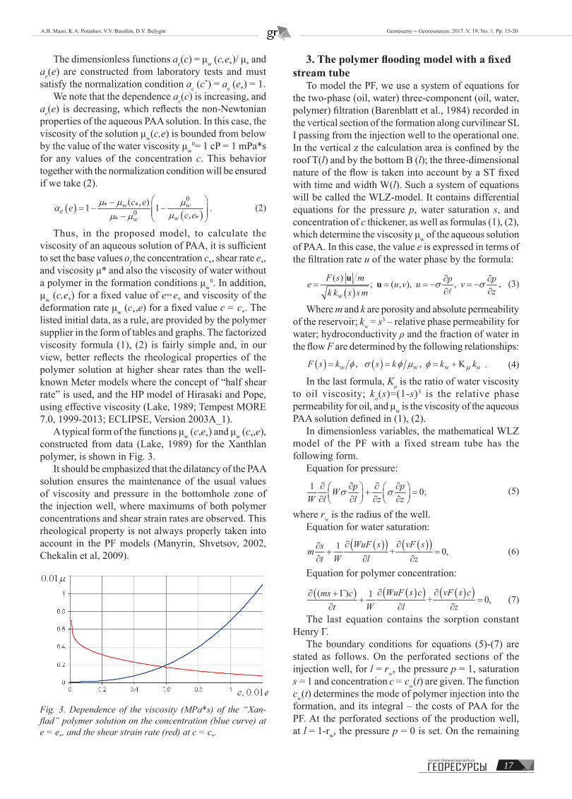
The dimensionless functions ac(c) = μw (c,e*)/ μ* and ae(e) are constructed from laboratory tests and must satisfy the normalization condition ac (c*) = ae (e*) = 1.

We note that the dependence ac(c) is increasing, and ae(e) is decreasing, which reflects the non-Newtonian properties of the aqueous PAA solution. In this case, the viscosity of the solution μw(c,e) is bounded from below by the value of the water viscosity μw

0= 1 cP = 1 mPa*s for any values of the concentration c. This behavior together with the normalization condition will be ensured if we take (2).

( ) ( )0

* *0

**

( , )1 1,

w we

ww

c eec e

µ µ µαµµ µ

−= − − −

. (2)

Thus, in the proposed model, to calculate the viscosity of an aqueous solution of PAA, it is sufficient to set the base values of the concentration c*, shear rate e*, and viscosity μ* and also the viscosity of water without a polymer in the formation conditions μw

0. In addition, μw (c,e*) for a fixed value of e=e* and viscosity of the deformation rate μw (c*,e) for a fixed value c = c*. The listed initial data, as a rule, are provided by the polymer supplier in the form of tables and graphs. The factorized viscosity formula (1), (2) is fairly simple and, in our view, better reflects the rheological properties of the polymer solution at higher shear rates than the well-known Meter models where the concept of “half shear rate” is used, and the HP model of Hirasaki and Pope, using effective viscosity (Lake, 1989; Tempest MORE 7.0, 1999-2013; ECLIPSE, Version 2003A_1).

A typical form of the functions μw (c,e*) and μw (c*,e), constructed from data (Lake, 1989) for the Xanthlan polymer, is shown in Fig. 3.

It should be emphasized that the dilatancy of the PAA solution ensures the maintenance of the usual values of viscosity and pressure in the bottomhole zone of the injection well, where maximums of both polymer concentrations and shear strain rates are observed. This rheological property is not always properly taken into account in the PF models (Manyrin, Shvetsov, 2002, Chekalin et al, 2009).

3. The polymer flooding model with a fixed stream tube

To model the PF, we use a system of equations for the two-phase (oil, water) three-component (oil, water, polymer) filtration (Barenblatt et al., 1984) recorded in the vertical section of the formation along curvilinear SL I passing from the injection well to the operational one. In the vertical z the calculation area is confined by the roof T(l) and by the bottom B (l); the three-dimensional nature of the flow is taken into account by a ST fixed with time and width W(l). Such a system of equations will be called the WLZ-model. It contains differential equations for the pressure p, water saturation s, and concentration of c thickener, as well as formulas (1), (2), which determine the viscosity μw of the aqueous solution of PAA. In this case, the value e is expressed in terms of the filtration rate u of the water phase by the formula:

( )( )

; ( , ), ,w

F s m p pe u v u vzk k s sm

σ σ∂ ∂= = = − = −

∂ ∂u

ul

, (3)

Where m and k are porosity and absolute permeability of the reservoir; kw = s3 – relative phase permeability for water; hydroconductivity ρ and the fraction of water in the flow F are determined by the following relationships:

( ) ( ), , Kw w w oF s k s k k kµφ σ φ µ φ= = = + . (4)

In the last formula, Kμ is the ratio of water viscosity to oil viscosity; ko(s)=(1-s)3 is the relative phase permeability for oil, and μw is the viscosity of the aqueous PAA solution defined in (1), (2).

In dimensionless variables, the mathematical WLZ model of the PF with a fixed stream tube has the following form.

Equation for pressure: 1 0;p pWW l l z z

σ σ∂ ∂ ∂ ∂ + = ∂ ∂ ∂ ∂ (5)

where rw is the radius of the well.Equation for water saturation: ( )( ) ( )( )1 + 0,

WuF s vF ssmt W l z

∂ ∂∂+ =

∂ ∂ ∂ (6)

Equation for polymer concentration: ( ) ( )( ) ( )( )( ) 1 + 0,

WuF s c vF s cms ct W l z

∂ ∂∂ + Γ+ =

∂ ∂ ∂ (7)

The last equation contains the sorption constant Henry Г.

The boundary conditions for equations (5)-(7) are stated as follows. On the perforated sections of the injection well, for l = rw, the pressure p = 1, saturation s = 1 and concentration c = cw(t) are given. The function cw(t) determines the mode of polymer injection into the formation, and its integral – the costs of PAA for the PF. At the perforated sections of the production well, at l = 1-rw, the pressure p = 0 is set. On the remaining

Fig. 3. Dependence of the viscosity (MPa*s) of the “Xan-flad” polymer solution on the concentration (blue curve) at e = e*, and the shear strain rate (red) at c = c*.


GEORESURSY18

sections of the boundary of calculated area, the waterproofing condition is set un = -σ∂p/∂n = 0.

The initial condition t = 0 : s = s0(1,z) for equation (6) describes the distribution of oil reserves in the studied vertical section of the formation at the time the PF starts. The only reliable way to determine the function s0(1,z) is the calculation of a full-scale geological-filtration model with an adaptation to the history of reservoir development (Kanevskaya, 2003). We use a super-element filtering model (Mazo, Bulygin, 2011; Mazo et al., 2013; Mazo et al., 2015) for this purpose, which allows solving this problem with the least expenditure of computing resources.

4. Evaluation of the efficiency of the polymer injection mode

The mathematical model (1)-(7) allows carrying out calculations of various PF scenarios, evaluating the effectiveness of the activity on a particular section of the deposit, and determining optimal development parameters. Let us give some results of numerical modeling of a three-layered reservoir in which the absolute permeability k of the upper layer is equal to 1, the middle layer is highly permeable, k = 10, and the lower one is weakly permeable, k = 0.1 (all quantities are dimensionless). At the moment t = 0 the layer is saturated with oil, s0(1, z) ≡ 0. Both wells are perfect for penetration. The process of oil displacement by aqueous solution of PAA in ST is simulated under five polymer injection modes described by the function cw(t) in the boundary condition on the left injection well.

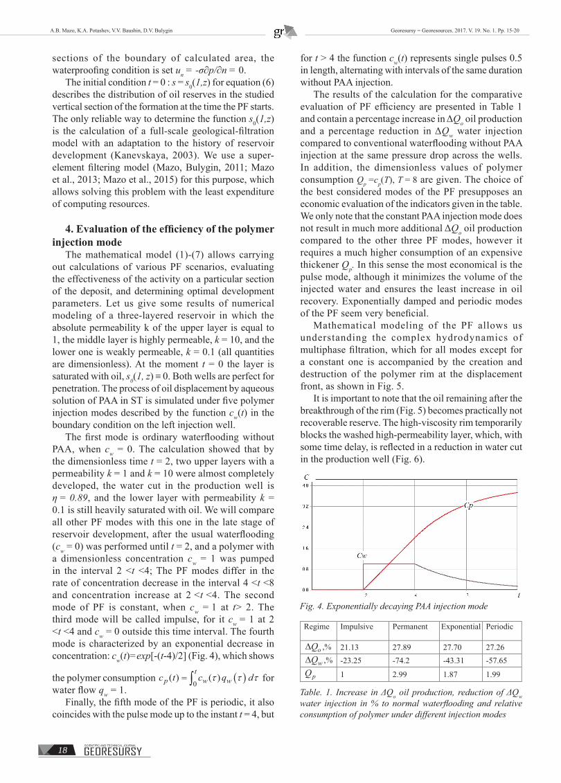
The first mode is ordinary waterflooding without PAA, when cw = 0. The calculation showed that by the dimensionless time t = 2, two upper layers with a permeability k = 1 and k = 10 were almost completely developed, the water cut in the production well is η = 0.89, and the lower layer with permeability k = 0.1 is still heavily saturated with oil. We will compare all other PF modes with this one in the late stage of reservoir development, after the usual waterflooding (cw = 0) was performed until t = 2, and a polymer with a dimensionless concentration cw = 1 was pumped in the interval 2 <t <4; The PF modes differ in the rate of concentration decrease in the interval 4 <t <8 and concentration increase at 2 <t <4. The second mode of PF is constant, when cw = 1 at t> 2. The third mode will be called impulse, for it cw = 1 at 2 <t <4 and cw = 0 outside this time interval. The fourth mode is characterized by an exponential decrease in concentration: cw(t)=exp[-(t-4)/2] (Fig. 4), which shows

the polymer consumption

( )0

( ) ( )t

p w wc t c q dτ τ τ= ∫ for water flow qw = 1.

Finally, the fifth mode of the PF is periodic, it also coincides with the pulse mode up to the instant t = 4, but

for t > 4 the function cw(t) represents single pulses 0.5 in length, alternating with intervals of the same duration without PAA injection.

The results of the calculation for the comparative evaluation of PF efficiency are presented in Table 1 and contain a percentage increase in ΔQo oil production and a percentage reduction in ΔQw water injection compared to conventional waterflooding without PAA injection at the same pressure drop across the wells. In addition, the dimensionless values of polymer consumption Qp =cp(T), T = 8 are given. The choice of the best considered modes of the PF presupposes an economic evaluation of the indicators given in the table. We only note that the constant PAA injection mode does not result in much more additional ΔQo oil production compared to the other three PF modes, however it requires a much higher consumption of an expensive thickener Qp. In this sense the most economical is the pulse mode, although it minimizes the volume of the injected water and ensures the least increase in oil recovery. Exponentially damped and periodic modes of the PF seem very beneficial.

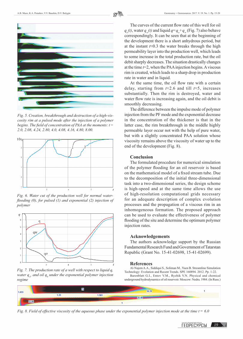
Mathematical modeling of the PF allows us understanding the complex hydrodynamics of multiphase filtration, which for all modes except for a constant one is accompanied by the creation and destruction of the polymer rim at the displacement front, as shown in Fig. 5.

It is important to note that the oil remaining after the breakthrough of the rim (Fig. 5) becomes practically not recoverable reserve. The high-viscosity rim temporarily blocks the washed high-permeability layer, which, with some time delay, is reflected in a reduction in water cut in the production well (Fig. 6).

Fig. 4. Exponentially decaying PAA injection mode

Table. 1. Increase in ΔQo oil production, reduction of ΔQw water injection in % to normal waterflooding and relative consumption of polymer under different injection modes

Regime Impulsive Permanent Exponential

Periodic

oQ∆ ,% 21.13 27.89 27.70 27.26

wQ∆ ,% -23.25 -74.2 -43.31 -57.65

pQ 1 2.99 1.87 1.99

19


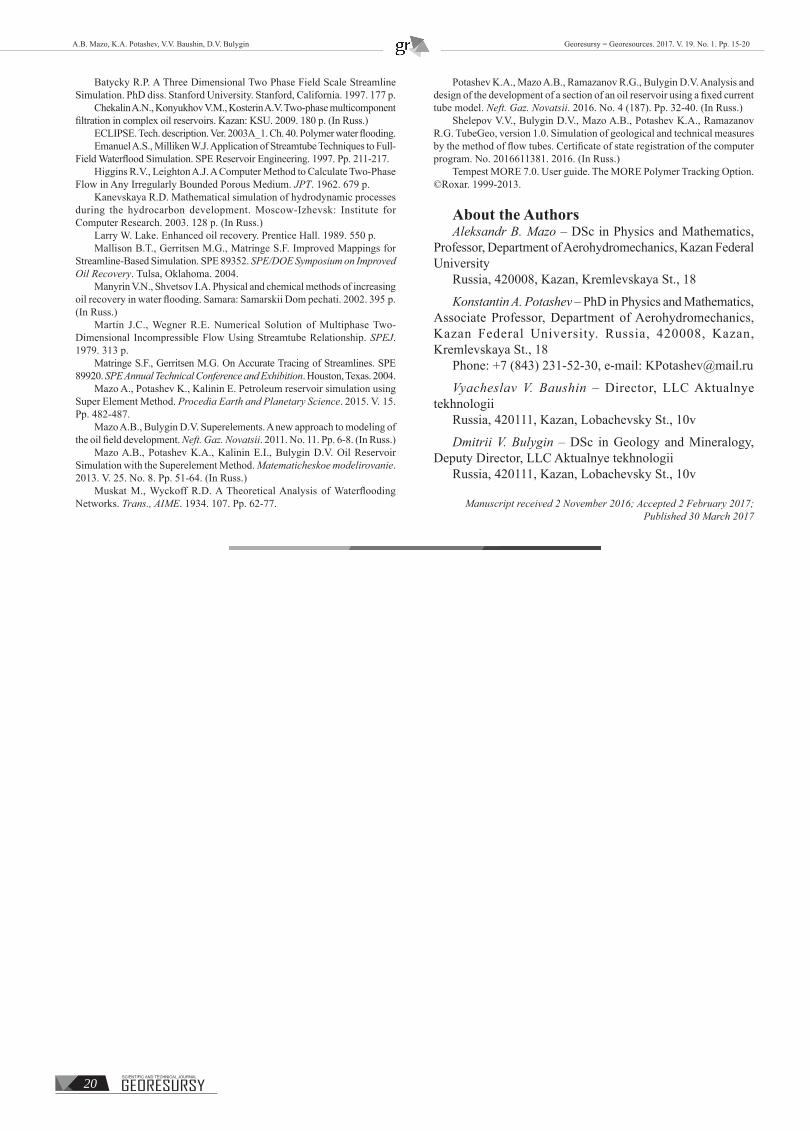
The curves of the current flow rate of this well for oil qo(t), water qw(t) and liquid q=qo+qw (Fig. 7) also behave correspondingly. It can be seen that at the beginning of the development there is a short anhydrous period, but at the instant t≈0.3 the water breaks through the high permeability layer into the production well, which leads to some increase in the total production rate, but the oil debit sharply decreases. The situation drastically changes at the time t=2, when the PAA injection begins. A viscous rim is created, which leads to a sharp drop in production rate in water and in liquid.

At the same time, the oil flow rate with a certain delay, starting from t≈2.6 and till t≈5, increases substantially. Then the rim is destroyed, water and water flow rate is increasing again, and the oil debit is smoothly decreasing.

The difference between the impulse mode of polymer injection from the PF mode and the exponential decrease in the concentration of the thickener is that in the latter case, the rim breakthrough in the middle highly permeable layer occur not with the help of pure water, but with a slightly concentrated PAA solution whose viscosity remains above the viscosity of water up to the end of the development (Fig. 8).

conclusionThe formulated procedure for numerical simulation

of the polymer flooding for an oil reservoir is based on the mathematical model of a fixed stream tube. Due to the decomposition of the initial three-dimensional task into a two-dimensional series, the design scheme is high-speed and at the same time allows the use of high-resolution computational grids necessary for an adequate description of complex evolution processes and the propagation of a viscous rim in an inhomogeneous formation. The proposed approach can be used to evaluate the effectiveness of polymer flooding of the site and determine the optimum polymer injection rates.

AcknowledgementsThe authors acknowledge support by the Russian

Fundamental Research Fund and Government of Tatarstan Republic (Grant No. 15-41-02698, 15-41-02699).

referencesAl-Najem A.A., Siddiqui S., Soliman M., Yuen B. Streamline Simulation

Technology: Evolution and Recent Trends. SPE 160894. 2012. Pp. 1-22.Barenblatt G.I., Entov V.M., Ryzhik V.N. Physical and chemical

underground hydrodynamics of oil reservoir. Moscow: Nedra. 1984. (In Russ.)

Fig. 8. Field of effective viscosity of the aqueous phase under the exponential polymer injection mode at the time t = 6.0

Fig. 7. The production rate of a well with respect to liquid q, water qw, and oil q0 under the exponential polymer injection regime

Fig. 6. Water cut of the production well for normal water-flooding (0), for pulsed (1) and exponential (2) injection of polymer

Fig. 5. Creation, breakthrough and destruction of a high-vis-cosity rim at a pulsed mode after the injection of a polymer begins. The field of concentration of PAA at the moments: t = 2.0, 2.08, 4.24, 2.80, 4.0, 4.08, 4.16, 4.80, 8.00.


GEORESURSY20

Batycky R.P. A Three Dimensional Two Phase Field Scale Streamline Simulation. PhD diss. Stanford University. Stanford, California. 1997. 177 p.

Chekalin A.N., Konyukhov V.M., Kosterin A.V. Two-phase multicomponent filtration in complex oil reservoirs. Kazan: KSU. 2009. 180 p. (In Russ.)

ECLIPSE. Tech. description. Ver. 2003A_1. Ch. 40. Polymer water flooding. Emanuel A.S., Milliken W.J. Application of Streamtube Techniques to Full-

Field Waterflood Simulation. SPE Reservoir Engineering. 1997. Pp. 211-217.Higgins R.V., Leighton A.J. A Computer Method to Calculate Two-Phase

Flow in Any Irregularly Bounded Porous Medium. JPT. 1962. 679 p.Kanevskaya R.D. Mathematical simulation of hydrodynamic processes

during the hydrocarbon development. Moscow-Izhevsk: Institute for Computer Research. 2003. 128 p. (In Russ.)

Larry W. Lake. Enhanced oil recovery. Prentice Hall. 1989. 550 p.Mallison B.T., Gerritsen M.G., Matringe S.F. Improved Mappings for

Streamline-Based Simulation. SPE 89352. SPE/DOE Symposium on Improved Oil Recovery. Tulsa, Oklahoma. 2004.

Manyrin V.N., Shvetsov I.A. Physical and chemical methods of increasing oil recovery in water flooding. Samara: Samarskii Dom pechati. 2002. 395 p. (In Russ.)

Martin J.C., Wegner R.E. Numerical Solution of Multiphase Two-Dimensional Incompressible Flow Using Streamtube Relationship. SPEJ. 1979. 313 p.

Matringe S.F., Gerritsen M.G. On Accurate Tracing of Streamlines. SPE 89920. SPE Annual Technical Conference and Exhibition. Houston, Texas. 2004.

Mazo A., Potashev K., Kalinin E. Petroleum reservoir simulation using Super Element Method. Procedia Earth and Planetary Science. 2015. V. 15. Pp. 482-487.

Mazo A.B., Bulygin D.V. Superelements. A new approach to modeling of the oil field development. Neft. Gaz. Novatsii. 2011. No. 11. Pp. 6-8. (In Russ.)

Mazo A.B., Potashev K.A., Kalinin E.I., Bulygin D.V. Oil Reservoir Simulation with the Superelement Method. Matematicheskoe modelirovanie. 2013. V. 25. No. 8. Pp. 51-64. (In Russ.)

Muskat M., Wyckoff R.D. A Theoretical Analysis of Waterflooding Networks. Trans., AIME. 1934. 107. Pp. 62-77.

Potashev K.A., Mazo A.B., Ramazanov R.G., Bulygin D.V. Analysis and design of the development of a section of an oil reservoir using a fixed current tube model. Neft. Gaz. Novatsii. 2016. No. 4 (187). Pp. 32-40. (In Russ.)

Shelepov V.V., Bulygin D.V., Mazo A.B., Potashev K.A., Ramazanov R.G. TubeGeo, version 1.0. Simulation of geological and technical measures by the method of flow tubes. Certificate of state registration of the computer program. No. 2016611381. 2016. (In Russ.)

Tempest MORE 7.0. User guide. The MORE Polymer Tracking Option. ©Roxar. 1999-2013.

about the authorsAleksandr B. Mazo – DSc in Physics and Mathematics,

Professor, Department of Aerohydromechanics, Kazan Federal University

Russia, 420008, Kazan, Kremlevskaya St., 18

Konstantin A. Potashev – PhD in Physics and Mathematics, Associate Professor, Department of Aerohydromechanics, Kazan Federal University. Russia, 420008, Kazan, Kremlevskaya St., 18

Phone: +7 (843) 231-52-30, e-mail: [email protected]

Vyacheslav V. Baushin – Director, LLC Aktualnye tekhnologii

Russia, 420111, Kazan, Lobachevsky St., 10v

Dmitrii V. Bulygin – DSc in Geology and Mineralogy, Deputy Director, LLC Aktualnye tekhnologii

Russia, 420111, Kazan, Lobachevsky St., 10v

Manuscript received 2 November 2016; Accepted 2 February 2017; Published 30 March 2017

Documents

Numerical SimulatioN of oil reServoir Polymer floodiNg by ... · 20 GEORESURSY University