Numerical Simulation of Fuel Filling with Volume of Fluid Master of Science Thesis [Innovative and Sustainable Chemical Engineering] Kristoffer Johansson Department of Chemistry and Bioscience Division of Chemical Reaction Engineering CHALMERS UNIVERSITY OF TECHNOLOGY Gothenburg, Sweden, 2011 Report No .xxx

Numerical Simulation of Fuel Filling with Volume of Fluid Masters Thesis Kristoffer Johansson © Kristoffer Johansson Department of Chemistry and Bioscience Chalmers University of Technology SE-412 96 Gothenburg Sweden Telephone +46(0)31-772 1000 Gothenburg, Sweden 2011 Picture on the front page describes the contour plot of volume fraction gasoline with an isosurface of the volume fraction gasoline, after 1s of fuel filling. The fuel filling is started when the tank is ~90% full.

Abstract The design of a new filling pipe and tank is often expensive and time consuming. The filling pipe is often costume made and if smaller changes are done in the geometry, a new filling pipe must be produced. It is therefore of interest of doing the preliminary investigation of a new fuel filling pipe with Computational Fluid Dynamics (CFD). The volume of fluid is an interface tracking method used for multiphase flow. The interface between gasoline and air is tracked by a color function and the interface is reconstructed in an implicit or explicit way. For the turbulence modeling Realizable k-ε with standard wall function is used. The experiments planned for verification of the numerical simulations failed. The transparent tank used for the experiments reacted with the gasoline and the filling pipe started to burst. Therefore the objective of the master thesis is changed from trying to develop a method for predicting fuel filling to a parameter study of the important parameters for modeling fuel filling. The important parameters are the mesh and time step size The different meshes investigated during this project are a tet mesh, different prism meshes and a hex mesh. All the prism meshes created for the project showed similar or better result in simulation of fuel filling than the tet mesh. Due to lack of time, the hex mesh is not fully investigated. The time step tested during the project was 2e-5s, 5e-6s and 2.5e-6s. The time step 2e-5s is proven to be too large for all the tested cases. Comparison between the other two time steps, 5e-6s and 2.5e-6s, showed little difference. The simulations indicate that it is possible to simulate fuel filling with volume of fluid. The implicit VOF discretization method is much more stable than the explicit VOF, and the implicit VOF is recommended as discretization method. The most promising mesh during the project is the fine 17 layers prism mesh with the time step 5e-6s.

Acknowledgments This thesis has been done at the CFD group at Volvo Car Corporation, Gothenburg. I would like to thank my supervisors at Volvo, Frida Nordin and Dr. Torbjörn Virdung for their patience and support during these months of hard work. I would also like to thank Patrik Sondell for improving my stamina, Marina Olsson for stepping in when my supervisors was away and the other guys at the CFD group for all the great time at the "fika" table. I would also like to thank Professor Bengt Andersson at Chalmers University of Technology for his support during this project and for that he has woken my interest for CFD. Most of all I would like to thank my future wife for her love, support and understanding. I am really looking forward to our marriage! Kristoffer Johansson Gothenburg, Sweden May 30, 2011

TABLE OF CONTENT 1. INTRODUCTION ................................................................................................................... 1

1.1 BACKGROUND ..................................................................................................................... 1 1.2 OBJECTIVE........................................................................................................................... 1

1.2.1 Original objective ........................................................................................................ 1 1.2.2 Revised objective......................................................................................................... 1

1.3 LIMITATIONS AND RESTRICTIONS ....................................................................................... 1 2. THEORY.................................................................................................................................. 2

2.1 TURBULENCE....................................................................................................................... 2 2.1.1 Governing equations.................................................................................................... 2

2.2 TURBULENCE MODELING .................................................................................................... 2 2.2.1 Reynolds decomposition and the RANS equations ..................................................... 2 2.2.2 The Boussinesq approximation ................................................................................... 3 2.2.3 Turbulence model ........................................................................................................ 4 2.3.3.1 Realizable k-ε model ................................................................................................ 5 2.3.4 Boundary Conditions ................................................................................................... 7 2.3.4.1 Inlet and outlet conditions ........................................................................................ 7 2.3.4.2 Wall functions........................................................................................................... 8

2.4 MULTIPHASE FLOW ............................................................................................................. 8 2.4.1 Volume of Fluid........................................................................................................... 8 2.4.2 Volume Fraction Equation......................................................................................... 10 2.4.2.1 Implicit discretization scheme ................................................................................ 10 2.4.2.2 Explicit discretization scheme ................................................................................ 10 2.4.2.3 Advection scheme................................................................................................... 11

2.5 MESHING ........................................................................................................................... 12 2.5.1 Courant Friedrichs Lewy condition ........................................................................... 12

2.6 NUMERICAL DIFFUSION..................................................................................................... 12 2.7 CONVERGENCE .................................................................................................................. 12

2.7.1 Enhancing convergence ............................................................................................. 13 2.7.2 Under-relaxation factor.............................................................................................. 13

2.8 SPATIAL DISCRETIZATION ................................................................................................. 14 2.8.1 Numerical scheme ..................................................................................................... 14 2.8.1.1 First order upwind scheme ..................................................................................... 14 2.8.1.2 Second order upwind scheme ................................................................................. 15 2.8.2 Pressure-velocity Coupling........................................................................................ 15

2.9 TEMPORAL DISCRETIZATION ............................................................................................. 16 2.9.1 Time advancement algorithm .................................................................................... 16

3. SIMULATIONS..................................................................................................................... 18 3.1 SOFTWARE......................................................................................................................... 18

3.1.1 Ansa ........................................................................................................................... 18 3.1.2 Ansys TGrid .............................................................................................................. 18 3.1.3 Ansys Fluent .............................................................................................................. 18 3.1.4 Ansys CFD-Post ........................................................................................................ 18

3.2 GEOMETRY ........................................................................................................................ 18 3.3 MESH ................................................................................................................................. 21

3.3.1 Tet mesh .................................................................................................................... 21 3.3.2 Prism mesh ................................................................................................................ 22 3.3.3 Hex mesh ................................................................................................................... 25

3.4 BOUNDARY CONDITIONS .................................................................................................. 26 3.5 MONITORING ..................................................................................................................... 27 3.6 PREVIOUS WORK................................................................................................................ 27

4. RESULTS............................................................................................................................... 29 4.1 MESH SIZE ......................................................................................................................... 29 4.2 TET MESH .......................................................................................................................... 29 4.3 CASE COMPARISON............................................................................................................ 31

4.3.1 Coarse prism mesh..................................................................................................... 31 4.3.2 Time step analysis, coarse prism mesh...................................................................... 34 4.3.3 Fine prism mesh......................................................................................................... 35 4.3.4 Time step analysis, fine prism mesh.......................................................................... 37 4.3.5 Extra fine prism mesh................................................................................................ 44 4.3.6 Time step analysis, extra fine prism mesh................................................................. 48 4.3.7 Numerical Scheme..................................................................................................... 48 4.3.8 Simulation time.......................................................................................................... 51 4.3.9 Hex mesh ................................................................................................................... 52

5. DISCUSSION......................................................................................................................... 54 5.1 MESH ................................................................................................................................. 54 5.2 EXPLICIT VS. IMPLICIT VOF.............................................................................................. 54 5.3 CASE COMPARISON............................................................................................................ 55

5.3.1 Coarse prism mesh..................................................................................................... 55 5.3.2 Time step, coarse prism mesh.................................................................................... 55 5.3.3 Fine prism mesh......................................................................................................... 55 5.3.4 Time step, fine prism mesh........................................................................................ 56 5.3.5 Extra fine prism mesh................................................................................................ 56 5.3.6 Numerical scheme ..................................................................................................... 57 5.3.7 Simulation time.......................................................................................................... 57 5.3.8 Hex mesh ................................................................................................................... 57

6. CONCLUSION AND RECOMMENDATION................................................................... 58 REFERENCES ..............................................................................................................................

1

1. INTRODUCTION 1.1 Background The design of a cars fuel filling system can be a very time consuming and expensive procedure. Often the fuel tank with filler pipe needs to be costume made and if small changes needed to be done to the geometry, a new tank or filler pipe must be produced. It is therefore of interest to do the preliminary testing of the fuel filling system with numerical simulation, like Computational Fluid Dynamic (CFD) to decrease lead time and cost in development of the fuel filling system.

1.2 Objective 1.2.1 Original objective The original objective for the project was to investigate the accuracy in predicting fuel filling with volume of fluid in CFD. The results from the simulations were supposed to be verified with experimental result preformed at the same geometry at Volvos Car Corporation's fuel department. An important parameter to investigate is the importance of having the fuel tank present in the simulation. If the fuel tank is replaced with just a pressure resistance the computational time can be reduced.

1.2.2 Revised objective Due to the lack of experiments, see 1.3 Limitations and Restrictions, the objective for the project has to be changed. Instead of trying to develop a method for predicting fuel filling, focus changed to investigate the important parameters during fuel filling. The important parameters are the mesh and the sizes of the time step used during the simulations.

1.3 Limitations and Restrictions The experiments for verification of the simulation did not go as well as expected. The material that the transparent tank was made of reacted with the gasoline and the filling pipe started to burst. Therefore there are no experimental results available for verification of the simulation and the objective for this maters thesis is changed. Time is also a limiting factor. This project time is set to 20 weeks and simulation time can with the denser meshes and smaller time step, be as long as a week. Due to the long simulation time, not all types of meshes and time step were investigated. The importance of having the tank present in the simulation is not either tested due to lack of time and experiments for verification of the simulation.

2

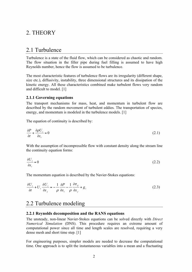
2. THEORY 2.1 Turbulence Turbulence is a state of the fluid flow, which can be considered as chaotic and random. The flow situation in the filler pipe during fuel filling is assumed to have high Reynolds number, hence the flow is assumed to be turbulence. The most characteristic features of turbulence flows are its irregularity (different shape, size etc.), diffusivity, instability, three dimensional structures and its dissipation of the kinetic energy. All these characteristics combined make turbulent flows very random and difficult to model. [1]

2.1.1 Governing equations The transport mechanisms for mass, heat, and momentum in turbulent flow are described by the random movement of turbulent eddies. The transportation of species, energy, and momentum is modeled in the turbulence models. [1] The equation of continuity is described by:

(2.1)

With the assumption of incompressible flow with constant density along the stream line the continuity equation forms:

(2.2)

The momentum equation is described by the Navier-Stokes equations:

(2.3)

2.2 Turbulence modeling 2.2.1 Reynolds decomposition and the RANS equations The unsteady, non-linear Navier-Stokes equations can be solved directly with Direct Numerical Simulation (DNS). This procedure requires an extreme amount of computational power since all time and length scales are resolved, requiring a very dense mesh and short time step. [1] For engineering purposes, simpler models are needed to decrease the computational time. One approach is to split the instantaneous variables into a mean and a fluctuating

3

part, letting the flow be statistically described by the mean flow velocity and the turbulence quantities. This method is called the Reynolds decomposition. [1]

(2.4)

(2.5) Using the Reynolds decomposition (eq. 2.4 and eq. 2.5) and the continuity equation for incompressible flow (eq. 2.2) in the Navier-Stokes equations (eq. 2.3) and taking a time-average the Reynolds Averaged Navier-Stokes (RANS) equation is obtained:

(2.6)

The difference between the original Navier-Stokes equations (eq. 2.3) and the RANS equations (eq. 2.6) lies in the additional term . [1] This term contains products of the velocity fluctuations and introduces a coupling between the mean and fluctuating parts of the velocity field. The term is referred to as the Reynolds stresses and requires modeling in order to close the RANS equations. The Reynolds stresses is a tensor and is individually described as:

(2.7)

The Reynolds stresses contains six unknown terms that require modeling, three normal stresses , and and three shear stresses ,

and . This because the tensor is symmetric, i.e. ,

and . [1]

2.2.2 The Boussinesq approximation One common method to model the Reynolds stresses is by assuming that the Reynolds stresses are proportional to the mean velocity gradient. This means that the transport of turbulence is assumed to be a diffusive process and that turbulent viscosity (eddy viscosity) can be used to model the Reynolds stress tensor. The concept is referred to as the Boussinesq approximation and is described by:

(2.8)

where υT is the turbulent viscosity k is the turbulent kinetic energy per unit mass

4

The turbulent kinetic energy is defined as . Note that the turbulent

viscosity is a property of the fluid flow not a property of the fluid like molecular viscosity, this means that it strongly depends on the state of turbulence. The Boussinesq approximation finally leads to:

(2.9)

Several limitations follow by using the Boussinesq approximation to model the Reynolds stresses. For example the method assumes that eddies behaves like molecules and exchange momentum quickly, that turbulence is isotropic and that local equilibrium exists between stress and strain. [1] When using the Boussinesq eddy-viscosity approximation to estimate the Reynolds stresses in the RANS equations, the turbulent eddy viscosity is introduced and requires modeling. The turbulent viscosity can be expressed as:

(2.10)

where u is the velocity l is the length scale To determine the turbulent eddy viscosity an additional set of equations are needed. The turbulence models that determine the eddy-viscosity can consist of a different amount of additional transport equations. The most common closure used for the RANS equations is the two-equation model. [1]

2.2.3 Turbulence model For general simulations of turbulence flow the two-equation models are often used due to their robustness and relative inexpensive computational cost. The two-equation models solve the turbulent velocity and length scale independently. The turbulence production and dissipation transportation can have localized rates. One approach to determine the local turbulence is to solve the turbulent kinetic energy (k) equation for the velocity scale and one equation with a property that can determine the length scale. Examples of properties are vorticity scale (ω), frequency scale (f), time scale (τ), dissipation rate (ε) and of course the length scales (l) itself. [1] The most common variable combination to describe the turbulence is to solve the k- and the ε-equation. This combination is called the k-ε model. The relation between turbulent energy dissipation and turbulent length scale is:

(2.11)

5

The length scale, l, is the turbulent velocity, times the lifetime of the turbulence

eddies :

(2.12)

The turbulent viscosity can then be determined by:

(2.13)

The most common and simple two-equation model is the standard k-ε model. It is a robust model with low computational cost. However with usage of the standard k-ε model some limitations follows. The accuracy describing round jets, swirls, flows involving significant curvature, sudden acceleration and low Reynolds regions is low. Accurate predictions can be made for high Reynolds numbers, isotropic turbulence, and flows where the energy cascade is in local equilibrium. Modifications can be made to the standard k-ε model to increase the applications. Examples of models are the RNG and realizable k-ε. However the standard k-ε is still a good model to start with due to its robustness. [1] In this project, the model used for predicting the turbulent structure of the flow is realizable k-ε. This is due to the significant curvature in the filling pipe that would have been difficult to resolve with standard k-ε.

2.3.3.1 Realizable k-ε model The exact transport equation for kinetic energy k with the Reynolds decomposition assumption is described by:

(2.14)

1 2 3 4 5 6 7 To be able to solve the exact transport equation for kinetic energy k closures are required. The unknown terms are the production (3), dissipation (4), and the diffusion terms (6 and 7). The production term is closed by using Boussinesq-approximation on the Reynolds stress term, by relating it to gradients of the mean flow. The dissipation term can be closed by the definition of the energy dissipation of turbulent kinetic energy. The diffusion terms, which must describe the turbulent transport of k, are closed by assuming a gradient diffusion transport mechanism. The three closures in the k-equation are defined as:

(2.15)

6

(2.16)

(2.17)

where σk is the Prandtl-Schmidt number. Submitting the closures (eq. 2.15–2.17) into the exact transport equation of kinetic energy (eq. 2.14), gives the modeled equation for k:

(2.18)

To solve the k-equation the energy dissipation rate, ε, and the turbulent viscosity, υT, needs to be determined. The exact transport of energy dissipation rate equation:

(2.19)

The exact equation of ε requires closures for the unknown terms, similar to the ones for the k equation 2.14, and finally the modeled ε-equation takes the form:

(2.20)

The time constant for turbulence is expressed as:

(2.21)

The rate of ε is proportional to:

(2.22)

The turbulent viscosity is given as the product of characteristic velocity and length scales, which will lead to the modeled form of υT:

(2.23)

7

The inaccuracy in this model comes from the use of the Boussinesq approximation that builds on the assumption of isotropic flow and the modeling method of the dissipation equation. [1] One limitation with the standard k-ε model is that the normal stress terms can become negative for flows with large mean strain rates (see eq. 2.24). This is unphysical since the normal stresses are a sum of squares and therefore must be positive. The normal stresses in the Reynolds stress tensor can be described as:

(2.24)

In realizable k-ε model a correction of the k-equation is made. This features a realizability constraint on the predicted stress tensor. The constant Cµ is changed to a variable to prevent the normal stresses to take negative values under all flow conditions, i.e. ensure realizability. This modification creates a model that should be able to predict flows involving rotation and separation more accurate. [1] The realizable k-ε model also modifies the ε-equation by adding a production term for turbulent energy dissipation. This change is considered to be the reason why the realizable k-ε model except for predicting planar jets, that the standard k-ε model can predict reasonably well, also resolves flows involving round jets. For simulations involving boundary layer flows, separated flows, and rotating shear flows the realizable k-ε model is preferable. It can better predict flows with a large strain rate. [1]

2.3.4 Boundary Conditions To be able to solve the turbulence models correctly proper boundary conditions must be specified. The system boundaries are the inlet, outlet and near the wall region.

2.3.4.1 Inlet and outlet conditions The choice of inlet and outlet conditions can have large influence on the simulation results and must therefore be carefully selected. The inlet and outlet velocity and turbulence is seldom constant, but rather depend on both upstream and downstream conditions. Therefore the inlet and outlet should be set far away from the region of interest so that the assumptions will not affect the final results. [1] For the realizable k-ε model, the turbulent kinetic energy and energy dissipation rate need inlet specifications. These quantities (k and ε) can be specified in terms of turbulent intensity and turbulent length scale. The turbulent intensity for a pipe at high Reynolds number is described by:

(2.25)

And the length scale by:

(2.26) where L is the hydraulic diameter

8

is the average velocity As outlet boundary condition the pressure is often set.

2.3.4.2 Wall functions In the region close to the wall viscous effects on the transport process are dominant. This implies that large gradients occur for the flow variables. Near the wall the “no-slip” condition, i.e. the relative velocity between the fluid and the wall is zero, applies. This condition applies since all the relevant momentum is lost when molecules hit the solid wall. Molecules that bounce back into the flow have then lost their momentum to the wall and the moving fluid close to the wall is slowed down, creating a boundary layer. Because of this, velocity increases rapidly from zero close to the wall up to free stream velocity. [1] For the models that cannot handle the near wall region wall functions can be used. The wall functions provide boundary conditions for the turbulent quantities and mean velocity components at the first grid point from the wall. This means that at the first cell close to the wall the velocities , k, ε and in the RANS models are provided. [1] The mean velocity components, the turbulent quantities and the Reynolds stresses are estimated from empirical rules based on the logarithmic law of the wall. This requires that the first grid point be within the logarithmic region, i.e. 20 < y+ 100. For flows involving strong pressure gradients, separation and impinging effects the validity of wall functions can be questioned. The distance to the first grid point, y+, is calculated as:

(2.27)

where y is the normal distance to the first grid point in the mesh, u* the characteristic velocity scale for the sub layer ν the kinematic viscosity

2.4 Multiphase flow As the most important flow situations for industrial application are turbulent, the most common flows are multiphase flows. Some of the common multiphase flows are rainfall, air pollution, boiling, flotation, fermentation, liquid-liquid extraction and spray drying. [2] Also fuel filling is a multiphase flow where fuel and air are the two different phases present.

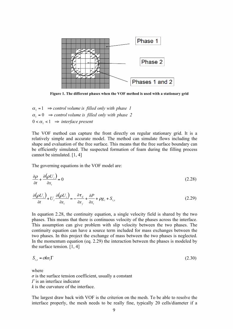
2.4.1 Volume of Fluid The idea with the volume of fluid (shorten VOF) method is that the interface between two phases is tracked. This is done by a color function (phase indicator function) that indicates the fractional amount of fluid at a certain position. [3] The different phases are illustrated in figure 1.

9

Figure 1. The different phases when the VOF method is used with a stationary grid

1 2

interface present The VOF method can capture the front directly on regular stationary grid. It is a relatively simple and accurate model. The method can simulate flows including the shape and evaluation of the free surface. This means that the free surface boundary can be efficiently simulated. The suspected formation of foam during the filling process cannot be simulated. [1, 4] The governing equations in the VOF model are:

(2.28)

(2.29)

In equation 2.28, the continuity equation, a single velocity field is shared by the two phases. This means that there is continuous velocity of the phases across the interface. This assumption can give problem with slip velocity between the two phases. The continuity equation can have a source term included for mass exchanges between the two phases. In this project the exchange of mass between the two phases is neglected. In the momentum equation (eq. 2.29) the interaction between the phases is modeled by the surface tension. [1, 4]

(2.30) where σ is the surface tension coefficient, usually a constant Γ is an interface indicator k is the curvature of the interface. The largest draw back with VOF is the criterion on the mesh. To be able to resolve the interface properly, the mesh needs to be really fine, typically 20 cells/diameter if a

10

bubble is resolved. The method is also of first order accurate; this is another reason for a use of a finer mesh. The problem with the cell size makes it impossible to resolve small bubbles or foam. [1, 4]

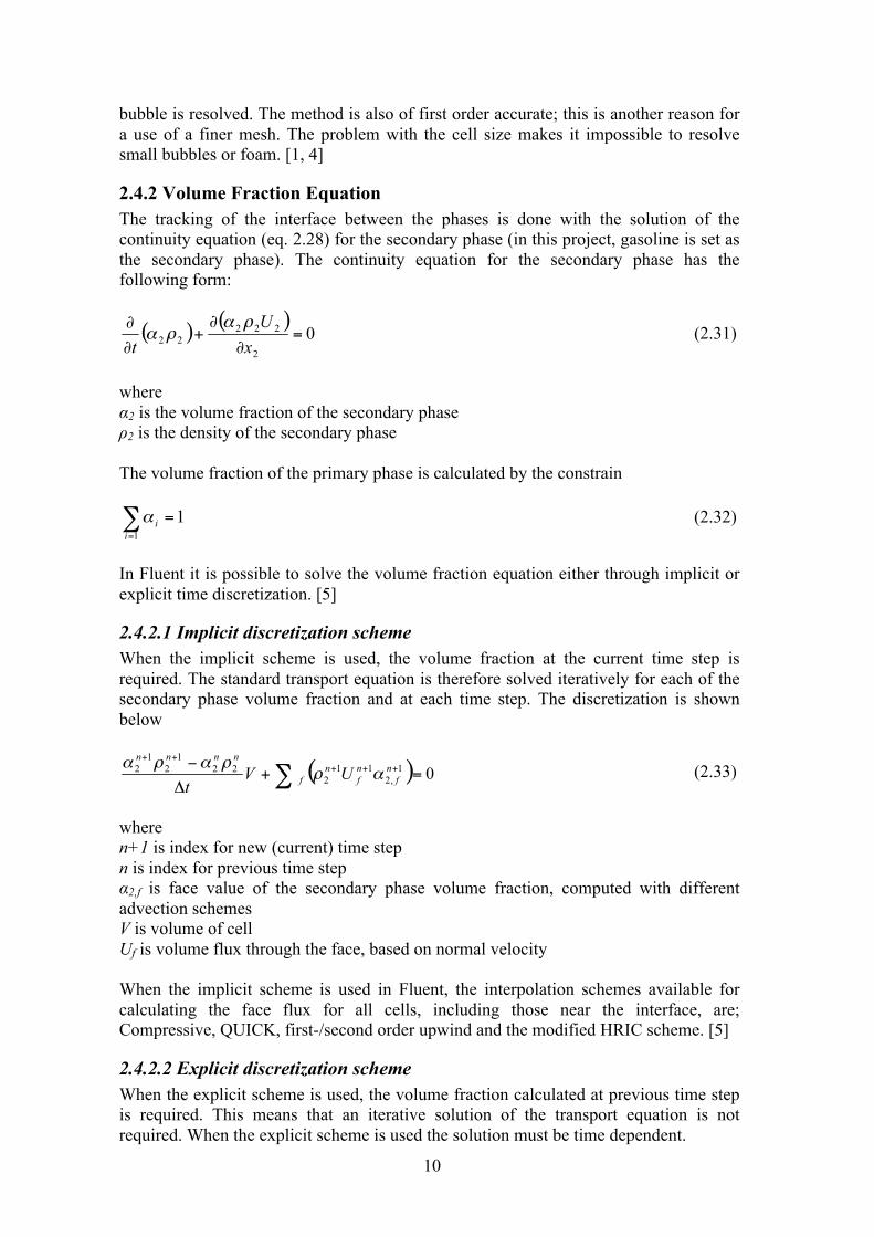
2.4.2 Volume Fraction Equation The tracking of the interface between the phases is done with the solution of the continuity equation (eq. 2.28) for the secondary phase (in this project, gasoline is set as the secondary phase). The continuity equation for the secondary phase has the following form:

(2.31)

where α2 is the volume fraction of the secondary phase ρ2 is the density of the secondary phase The volume fraction of the primary phase is calculated by the constrain

(2.32)

In Fluent it is possible to solve the volume fraction equation either through implicit or explicit time discretization. [5]

2.4.2.1 Implicit discretization scheme When the implicit scheme is used, the volume fraction at the current time step is required. The standard transport equation is therefore solved iteratively for each of the secondary phase volume fraction and at each time step. The discretization is shown below

(2.33)

where n+1 is index for new (current) time step n is index for previous time step α2,f is face value of the secondary phase volume fraction, computed with different advection schemes V is volume of cell Uf is volume flux through the face, based on normal velocity When the implicit scheme is used in Fluent, the interpolation schemes available for calculating the face flux for all cells, including those near the interface, are; Compressive, QUICK, first-/second order upwind and the modified HRIC scheme. [5]

2.4.2.2 Explicit discretization scheme When the explicit scheme is used, the volume fraction calculated at previous time step is required. This means that an iterative solution of the transport equation is not required. When the explicit scheme is used the solution must be time dependent.

11

(2.34)

where n+1 is index for new (current) time step n is index for previous time step α2,f is face value of the secondary phase volume fraction, computed with different advection schemes V is volume of cell Uf is volume flux through the face, based on normal velocity There are two possible interpolation methods available in Fluent when an explicit time discretization is used. The face flux can either be interpolated using interface reconstruction or be interpolated using a finite volume discretization scheme. The available reconstruction schemes in Fluent are Geo-Reconstruct and Donor-Acceptor. The finite volume discretization schemes available in Fluent are; first-/second order upwind, CICSAM, Compressive, Modified HRIC and QUICK. [5]

2.4.2.3 Advection scheme The advection schemes (interface interpolation scheme) are needed to keep the interface sharp and to produce monotonic profiles of the color function. When choosing advection scheme, the order of the scheme is important. Lower order scheme, like first order upwind, can give problem with numerical diffusion, which will smear, out the interface. Higher order schemes can be unstable and give problem with numerical oscillations. [1, 4] The interface that is calculated with eq. 2.31 is reconstructed during this project with two different schemes, the Geo-Reconstruction scheme and Modified HRIC scheme. The Geo-Reconstruction scheme is used with the explicit VOF, it is not available with the implicit VOF and instead Modified HRIC is used with the implicit VOF. The geometric reconstruction scheme uses a piecewise linear approach to reconstruct the interface between the phases. It assumes that the interface between two phases has a linear slope within the cell. This linear shape is used to calculate the advection of the fluid through the cell faces. This scheme is the most accurate for reconstruction of the interface but it is more computational expensive than the other discretization scheme available in Fluent. [5] The Modified HRIC is a central differencing scheme. The central differencing scheme is preferred before the upwind schemes when a VOF simulation is preformed. This is because of the overlay diffusive nature of the upwind schemes. On the other hand, the central differencing scheme is unbound and can give unphysical results. This problem is overcome using High Resolution Interface Capturing (HRIC). The Modified HRIC consists of a non-linear mix of upwind and downwind differencing. The modified HRIC scheme provides more accuracy than the other face flux scheme available in Fluent (QUICK, first-/ second order upwind for implicit solver) and is less computational expensive than the Geo-Reconstruction scheme. [5, 7]

12

2.5 Meshing One of the most important features in a good CFD simulation is the mesh. The grid is usually divided into structural grids and unstructured grid. The structural grid is build up by four edged elements but not necessary rectangles. In this arrangement, indexing and finding neighboring cells are very easy. Therefore a structured grid is often faster and requires less memory than if an unstructured grid is used. However it is not always possible to mesh complex geometries with a structured grid. [1] There are some restrictions of the appearance of the mesh to improve the accuracy of the solution. For elements close to the walls the angle between the wall and the grid should be close to 90o. The ratio of adjacent cell size should not be less than two and the aspect ratio of a computational cell less than five. The skewness of the computational cell should be greater than 45o. [1]

2.5.1 Courant Friedrichs Lewy condition For transient simulation there exists relation between the size of the computational cell, the transient time step size and the local fluid velocity within the cell. The relation is calculated by the CFL (Courant-Friedrichs-Lewy) equation:

(2.35)

where Δt is the time step used during the simulation Δxcell is the size of one side of the cell vcell is the velocity in the cell When an explicit solver is used, the CFL number (also called the courant number) can be used as a criterion for convergence but in this project the CFL number is just used as a measure for stability. [7]

2.6 Numerical diffusion Numerical diffusion, also called false diffusion, can occur when the flow situation is dominated by convection, i.e. the real diffusion is small. It can also occur when the cells are not parallel to the flow, which will lead to transport of species due to discretization. The numerical diffusion is minimized if the cells are parallel to the flow, the mesh is refined (since numerical diffusion has an inversely relation to the mesh resolution), and a higher order discretization scheme is used. [1]

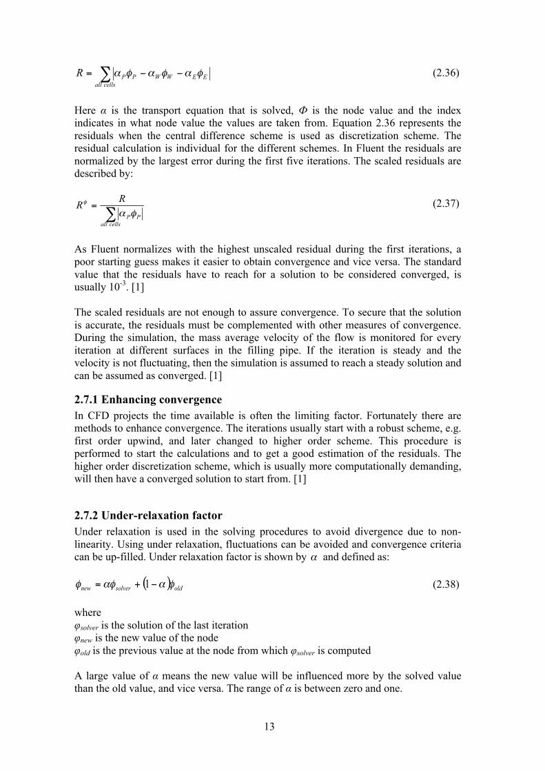
2.7 Convergence An important feature when performing CFD simulations is to know when the right solution is obtained, i.e. when the solution is converged, and the CFD simulation can be stopped. Since the exact solution of the problem is unknown, it is not possible to compare the numerical solution with the exact. Fluent uses user defined residuals to stop the iteration. The residual is a measurement of the absolute error. The residual is expressed as:

13

(2.36)

Here α is the transport equation that is solved, Ф is the node value and the index indicates in what node value the values are taken from. Equation 2.36 represents the residuals when the central difference scheme is used as discretization scheme. The residual calculation is individual for the different schemes. In Fluent the residuals are normalized by the largest error during the first five iterations. The scaled residuals are described by:

(2.37)

As Fluent normalizes with the highest unscaled residual during the first iterations, a poor starting guess makes it easier to obtain convergence and vice versa. The standard value that the residuals have to reach for a solution to be considered converged, is usually 10-3. [1] The scaled residuals are not enough to assure convergence. To secure that the solution is accurate, the residuals must be complemented with other measures of convergence. During the simulation, the mass average velocity of the flow is monitored for every iteration at different surfaces in the filling pipe. If the iteration is steady and the velocity is not fluctuating, then the simulation is assumed to reach a steady solution and can be assumed as converged. [1]

2.7.1 Enhancing convergence In CFD projects the time available is often the limiting factor. Fortunately there are methods to enhance convergence. The iterations usually start with a robust scheme, e.g. first order upwind, and later changed to higher order scheme. This procedure is performed to start the calculations and to get a good estimation of the residuals. The higher order discretization scheme, which is usually more computationally demanding, will then have a converged solution to start from. [1]

2.7.2 Under-relaxation factor Under relaxation is used in the solving procedures to avoid divergence due to non-linearity. Using under relaxation, fluctuations can be avoided and convergence criteria can be up-filled. Under relaxation factor is shown by and defined as:

(2.38) where φsolver is the solution of the last iteration φnew is the new value of the node φold is the previous value at the node from which φsolver is computed A large value of α means the new value will be influenced more by the solved value than the old value, and vice versa. The range of α is between zero and one.

14

2.8 Spatial discretization To construct values of scalar at the cell face, spatial discretization is needed. It is also necessary for computing velocity derivates and secondary diffusion terms. The gradient

of a given variable is used to discretize the convection and diffusion term in the flow conservation equation. [5] Three different gradient discretization schemes are available in Fluent, Green-Gauss Cell-based, Green-Gauss Node-based and Least Squares Cell-based. The Green-Gauss node–based is used in this project hence it is the only one further explained. [5] The Green-Gauss Node-based scheme computes the gradient of a scalar at the cell center c0 with the following discrete equation:

(2.39)

Where the summation is over all faces enclosing the cell and is the value of at

the cell face centroid. For the node-based equation, is calculated as:

(2.40)

where Nf is the number of nodes on the face The nodal value, , is calculated from the weighted average of the cell values surrounding the nodes. The node-based gradient is known to be more accurate than the cell-based gradient particularly on irregular unstructured meshes but it is more computational expensive than the cell-based gradient scheme. [5]

2.8.1 Numerical scheme To get accurate simulation results, the choice of numerical scheme is almost as important as the choice of turbulent model. Desired properties of the discretization scheme are to upheld boundedness and transportiveness

2.8.1.1 First order upwind scheme The first order upwind scheme transport information by setting the face value between two nodes equal to the nearest upstream node value:

(2.41) The gradients are estimated as:

(2.42)

15

From the equations it can be seen that the first order upwind scheme is bounded and it also fulfills the requirement of transportiveness since the direction of the flow is taken into account. The downside with this scheme is that it overestimates the transport in the flow direction, hence gives rise to numerical diffusion. However, if the flow is aligned with the mesh the numerical diffusion decreases and the first order upwind scheme is a good choice. The first order upwind discretization scheme also provides accurate results for flows where convection is dominating. The boundeness and robust properties make the first order upwind scheme a good starting scheme. However, for final simulations it should be replaced with higher order schemes. [1]

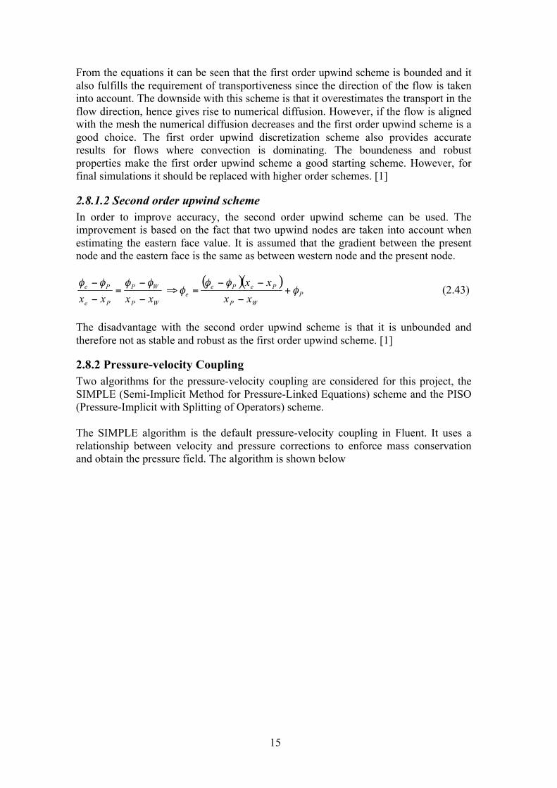
2.8.1.2 Second order upwind scheme In order to improve accuracy, the second order upwind scheme can be used. The improvement is based on the fact that two upwind nodes are taken into account when estimating the eastern face value. It is assumed that the gradient between the present node and the eastern face is the same as between western node and the present node.

(2.43)

The disadvantage with the second order upwind scheme is that it is unbounded and therefore not as stable and robust as the first order upwind scheme. [1]

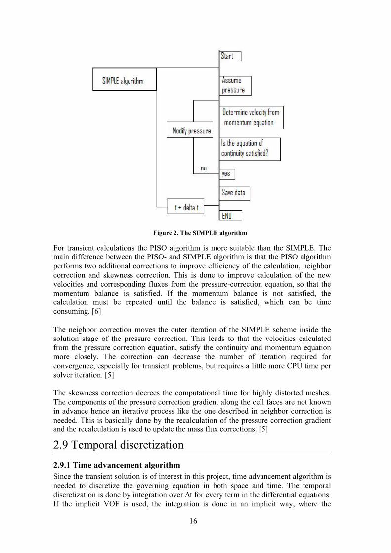
2.8.2 Pressure-velocity Coupling Two algorithms for the pressure-velocity coupling are considered for this project, the SIMPLE (Semi-Implicit Method for Pressure-Linked Equations) scheme and the PISO (Pressure-Implicit with Splitting of Operators) scheme. The SIMPLE algorithm is the default pressure-velocity coupling in Fluent. It uses a relationship between velocity and pressure corrections to enforce mass conservation and obtain the pressure field. The algorithm is shown below

16

Figure 2. The SIMPLE algorithm

For transient calculations the PISO algorithm is more suitable than the SIMPLE. The main difference between the PISO- and SIMPLE algorithm is that the PISO algorithm performs two additional corrections to improve efficiency of the calculation, neighbor correction and skewness correction. This is done to improve calculation of the new velocities and corresponding fluxes from the pressure-correction equation, so that the momentum balance is satisfied. If the momentum balance is not satisfied, the calculation must be repeated until the balance is satisfied, which can be time consuming. [6] The neighbor correction moves the outer iteration of the SIMPLE scheme inside the solution stage of the pressure correction. This leads to that the velocities calculated from the pressure correction equation, satisfy the continuity and momentum equation more closely. The correction can decrease the number of iteration required for convergence, especially for transient problems, but requires a little more CPU time per solver iteration. [5] The skewness correction decrees the computational time for highly distorted meshes. The components of the pressure correction gradient along the cell faces are not known in advance hence an iterative process like the one described in neighbor correction is needed. This is basically done by the recalculation of the pressure correction gradient and the recalculation is used to update the mass flux corrections. [5]

2.9 Temporal discretization 2.9.1 Time advancement algorithm Since the transient solution is of interest in this project, time advancement algorithm is needed to discretize the governing equation in both space and time. The temporal discretization is done by integration over ∆t for every term in the differential equations. If the implicit VOF is used, the integration is done in an implicit way, where the

17

equation is solved iteratively at each time level before moving to the next time step. The advantage of the implicit scheme is that it is stable with respect to time step size. [5] When the explicit VOF is used, explicit time integration is available. The time step, when using explicit time integration, is restricted to the stability limit of the underlying solver i.e. the time step is limited by the courant number. For stability, the explicit time stepping uses global time stepping. The global time stepping make sure that all cells in the domain must use the same time step and that time step must be the minimum of all the local time steps in the domain. The use of this time stepping has some restriction, but to capture the transient behavior of moving waves it can be more accurate and less expensive than implicit time stepping. But the CFL criterion for stability (CFL<0.5) makes the time stepping sensitive to sudden acceleration of the fluid and therefore very small time steps can be needed hence make the simulation time consuming. [5]

18

3. SIMULATIONS 3.1 Software 3.1.1 Ansa Ansa is a CAE pre-processing tool used for cleaning up the CAD models. The CAD model is often rather crude and needs to be clean up before meshing. The software can also create surface and volume meshes. [8]

3.1.2 Ansys TGrid Ansys TGrid is a software for creating surface and volume meshes. In this project, the surface mesh is imported from Ansa and the volume mesh is created in TGrid. The software offers advanced prism layer creation tool that includes sharp corner handling. The quality of the mesh is easily checked with inbuilt diagnostic program. [9]

3.1.3 Ansys Fluent Ansys Fluent is a simulation software for modeling fluid flow, heat transfer and chemical reaction. Fluent is used for all numerical simulation in this project. In Fluent, the different turbulence models, multiphase models, discretization schemes and time- /length steps are specified. [10]

3.1.4 Ansys CFD-Post Ansys CFD-Post is a post-processing software. It can generate 2D and 3D images, comparison between two different simulation results, where the difference between the results can easily be seen. It can also create animation if a transient solution is exported from Fluent. [11]

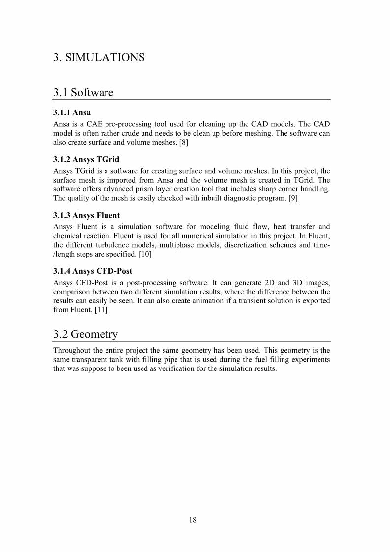
3.2 Geometry Throughout the entire project the same geometry has been used. This geometry is the same transparent tank with filling pipe that is used during the fuel filling experiments that was suppose to been used as verification for the simulation results.

19

Figure 3. The tank and fuel filling pipe geometry

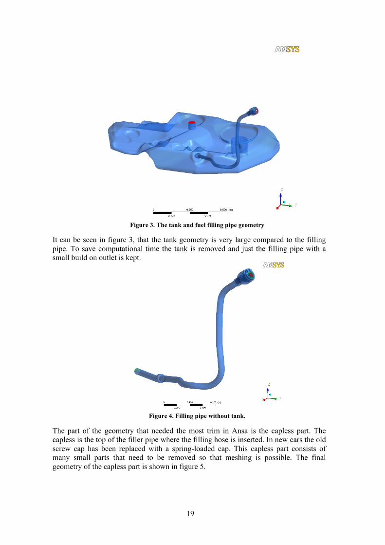
It can be seen in figure 3, that the tank geometry is very large compared to the filling pipe. To save computational time the tank is removed and just the filling pipe with a small build on outlet is kept.

Figure 4. Filling pipe without tank.

The part of the geometry that needed the most trim in Ansa is the capless part. The capless is the top of the filler pipe where the filling hose is inserted. In new cars the old screw cap has been replaced with a spring-loaded cap. This capless part consists of many small parts that need to be removed so that meshing is possible. The final geometry of the capless part is shown in figure 5.

20

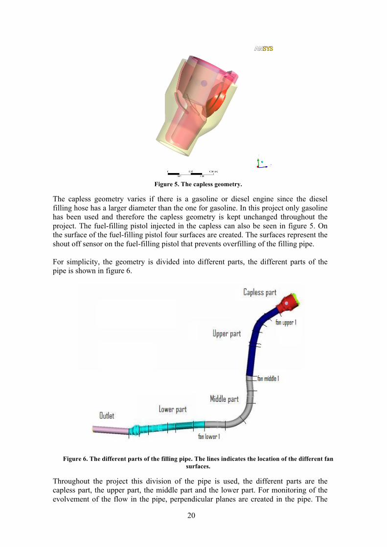
Figure 5. The capless geometry.

The capless geometry varies if there is a gasoline or diesel engine since the diesel filling hose has a larger diameter than the one for gasoline. In this project only gasoline has been used and therefore the capless geometry is kept unchanged throughout the project. The fuel-filling pistol injected in the capless can also be seen in figure 5. On the surface of the fuel-filling pistol four surfaces are created. The surfaces represent the shout off sensor on the fuel-filling pistol that prevents overfilling of the filling pipe. For simplicity, the geometry is divided into different parts, the different parts of the pipe is shown in figure 6.

Figure 6. The different parts of the filling pipe. The lines indicates the location of the different fan

surfaces.

Throughout the project this division of the pipe is used, the different parts are the capless part, the upper part, the middle part and the lower part. For monitoring of the evolvement of the flow in the pipe, perpendicular planes are created in the pipe. The

21

surfaces are called fans and are named depending on where in the pipe they are located, see figure 6. The number of the different fans is counted from the capless and down; example fan upper 1 is the first plane in the upper part of the pipe.

3.3 Mesh Three different types of meshes are created for this project and two of them are fully investigated. The meshes are tetrahedron mesh (shorten tet mesh), prism /tetrahedron mesh (prism mesh) and hexahedron mesh (hex mesh). The different types of meshes are shown in table 1.

Table 1. The different types of meshes created for the project.

Mesh type Tet

Prism 5 layers Prism 10 layers Prism 17 layers

Fine prism 10 layers Fine prism 17 layers

Extra fine prism 17 layers Hex

The meshes shown in table 1 also act as case name for the different cases. In this chapter the creation of the different meshes are explained.

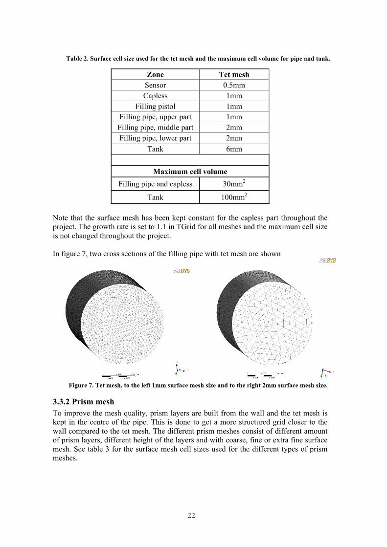
3.3.1 Tet mesh A tet mesh is very easy to generate and can give a good structural result. The tet mesh in this project is created with almost the same surfaces mesh as the mesh used in previous work (see 3.6 Previous work) on fuel filling at Volvo Cars. The surface mesh is created in Ansa and the volume mesh is created in TGrid. In table 2, the surface mesh size in the different parts of the pipe and the maximum cell volume for the tet mesh are shown.

22

Table 2. Surface cell size used for the tet mesh and the maximum cell volume for pipe and tank.

Zone Tet mesh Sensor 0.5mm Capless 1mm

Filling pistol 1mm Filling pipe, upper part 1mm

Filling pipe, middle part 2mm Filling pipe, lower part 2mm

Tank 6mm

Maximum cell volume Filling pipe and capless 30mm2

Tank 100mm2 Note that the surface mesh has been kept constant for the capless part throughout the project. The growth rate is set to 1.1 in TGrid for all meshes and the maximum cell size is not changed throughout the project. In figure 7, two cross sections of the filling pipe with tet mesh are shown

Figure 7. Tet mesh, to the left 1mm surface mesh size and to the right 2mm surface mesh size.

3.3.2 Prism mesh To improve the mesh quality, prism layers are built from the wall and the tet mesh is kept in the centre of the pipe. This is done to get a more structured grid closer to the wall compared to the tet mesh. The different prism meshes consist of different amount of prism layers, different height of the layers and with coarse, fine or extra fine surface mesh. See table 3 for the surface mesh cell sizes used for the different types of prism meshes.

23

Table 3. Surface cell size used for the different types of prism meshes.

Zone Coarse prism mesh

Fine prism mesh

Extra fine prism mesh

Sensor 0.5mm 0.5mm 0.5mm Capless 1mm 1mm 1mm

Filling pistol 2-3mm 1mm 1mm Filling pipe, upper part 2-3mm 1mm 0.75mm

Filling pipe, middle part 2-3mm 2mm 2mm Filling pipe, lower part 2-3mm 2mm 2mm

Tank 6mm 6mm 6mm The prism layer is created so that the height of the prism is the same as the height of the tet cell close to the wall, for the tet mesh with 1mm surface mesh.

Figure 8. Tetrahedron geometry.

It is assumed that the distances A-B, A-C, A-D, B-C and C-D is the same length, a=1mm. The height of the tetrahedron can be calculated as:

(3.1)

This height, h=0.8mm, is set as the height of the prism cells for the meshes with 5 prism layers and with 10 prism layers. The height of the prism is also made lower, to make the prism mesh finer. The lower height of the prism is calculated so that the mesh satisfies the y+ criterion for the wall function (see. 2.3.4.2 Wall Function). Equation 2.27 is used with the result from the simulation with the fine prism 10 layers.

(3.2)

If u and υ is assumed to be constant if the mesh is refined, y1

+=35 (from simulation) and y1=0.8. If y2

+ is set to 20 then y2, the height of the prism layer, can be calculated as:

(3.3)

24

So to remain within the region of the wall function, the height of the prism is set to 0.46 mm. This height is used for the meshes with 17 prism layers. The prism meshes created with the coarse surface mesh and the different layers of prism are shown in figures 9 and 10.

Figure 9. Prism 5 layers to the right and to the left prism 10 layers, both created from the coarse surface

mesh.

Figure 10. Prism 17 layers created from the coarse surface mesh.

Two prism meshes are created with finer surface mesh, prism 10 layers and prism 17 layers. The two different fine prism meshes are shown in figure 11.

25

Figure 11. Fine prism 10 layers to the left and fine prim 17 layers to the right, both meshes are created

from the fine surface mesh.

Finally a mesh is created with the extra fine surface mesh in the upper part of the pipe and 17 prism layers. This mesh is shown in figure 12.

Figure 12. Extra fine prism 17 layers created from the extra fine surface mesh.

The extra fine prism 17 layers are the densest mesh created during this project.

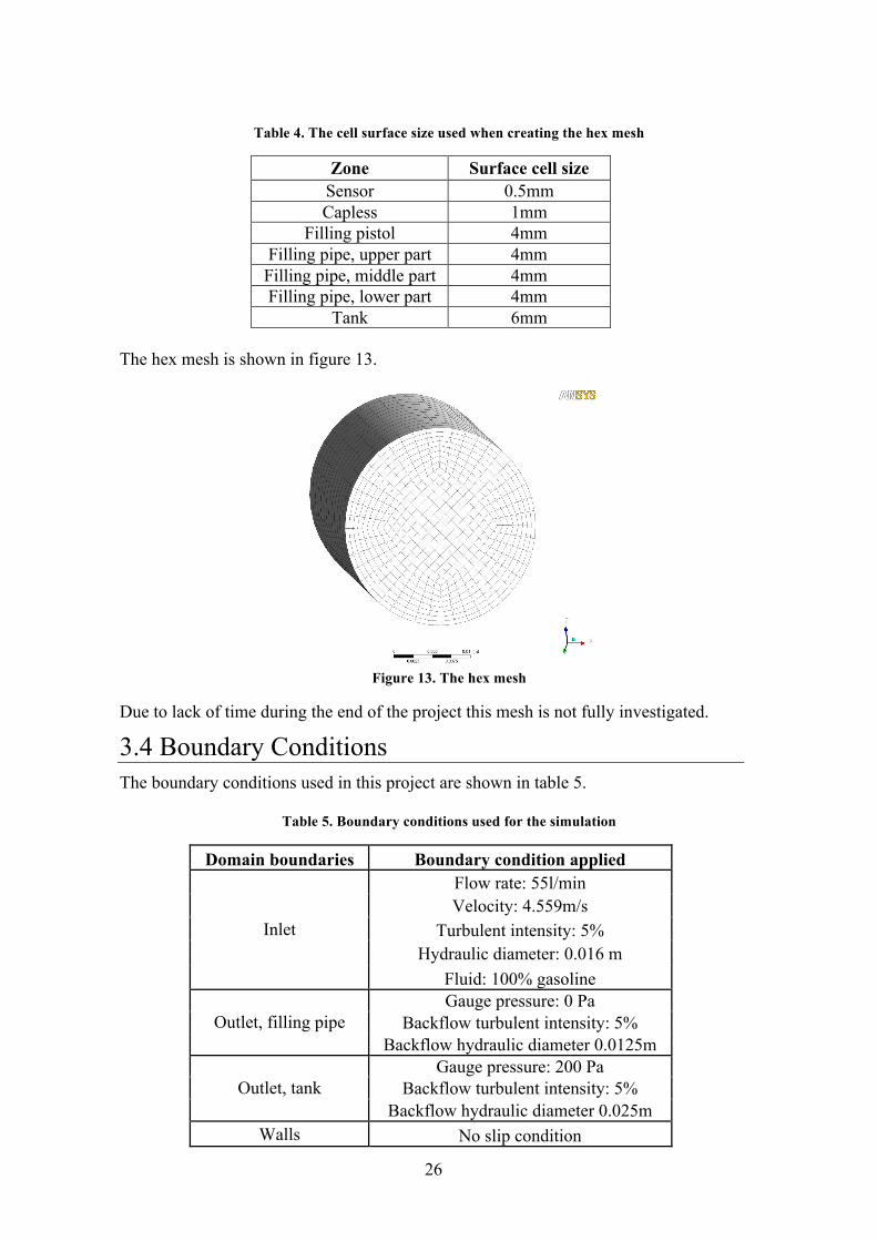
3.3.3 Hex mesh Instead of using tet cells or prism cells to create a mesh, hex cells can be used. The pipe geometry is rather fine, meaning the bends are not to sharp so there should be no problem in creating a hex mesh. The meshing is done in Ansa. The capless is not meshed with hex cells; it still has a tet mesh. In table 4 the surface cell size for the hex mesh is shown.

26

Table 4. The cell surface size used when creating the hex mesh

Zone Surface cell size Sensor 0.5mm Capless 1mm

Filling pistol 4mm Filling pipe, upper part 4mm

Filling pipe, middle part 4mm Filling pipe, lower part 4mm

Tank 6mm The hex mesh is shown in figure 13.

Figure 13. The hex mesh

Due to lack of time during the end of the project this mesh is not fully investigated.

3.4 Boundary Conditions The boundary conditions used in this project are shown in table 5.

Table 5. Boundary conditions used for the simulation

Domain boundaries Boundary condition applied Flow rate: 55l/min Velocity: 4.559m/s

Turbulent intensity: 5% Hydraulic diameter: 0.016 m

Inlet

Fluid: 100% gasoline Gauge pressure: 0 Pa

Backflow turbulent intensity: 5% Outlet, filling pipe Backflow hydraulic diameter 0.0125m

Gauge pressure: 200 Pa Backflow turbulent intensity: 5% Outlet, tank

Backflow hydraulic diameter 0.025m Walls No slip condition

27

3.5 Monitoring To investigate the flow situation in the pipe, the facet average of the volume fraction of gasoline is monitored at the fan surfaces in the pipe. The volume fraction gasoline is also monitored at the shut off sensors on the fuel-filling pistol. The CFL number will be monitored at the upper part of the pipe to investigate the connection between time step sizes, mesh size and cell velocity. The upper part is monitored because the mesh is smallest in this region and therefore the CFL number is assumed to be largest. To ensure convergence, the average velocity is monitored every iteration at three different fans in the pipe. If the flow is stable, not oscillating, then it is assumed that a stable solution is reached and the simulation within the time step has converged. To investigate the transient behavior of the flow, automatic export to CFD-Post of the volume fraction gasoline is done. The export is set to every 250 time step.

3.6 Previous work The initial settings for this project are based on previous simulation of fuel filling preformed at Volvo Car Corporation [12]. The boundary condition for the simulation is show in table 6.

Table 6. Boundary condition used in the previous work.

Domain boundaries Boundary condition applied Flow rate: 55l/min

Turbulent intensity: 5% Hydraulic diameter: 0.019 m Inlet

Fluid: 100% diesel Gauge pressure: 0 Pa

Backflow turbulent intensity: 5% Outlet, filling pipe Backflow hydraulic diameter 0.065m

Gauge pressure: 0 Pa Backflow turbulent intensity: 5% Outlet, tank

Backflow hydraulic diameter 0.05m Walls No slip condition

The mesh used during the computation is a tet mesh. The surface cell sizes are shown in table 7.

28

Table 7. Surface cell sizes used for the tet mesh created during previous work.

Zone Surface cell size Pistol sensor 0.5mm

Fuel-filling pistol 1 mm Filling pipe, upper part 1 mm

Filling pipe, middle part 2 mm Filling pipe, part closest to tank 3 mm

Tank 6 mm The maximum cell volume in TGrid is set to 30mm2 for the filling pipe and 100mm2 for the tank. [12] The time step used for the simulation is 2e-5s and the explicit volume fraction discretization is used.

29

4. RESULTS The investigation of the simulation in this project follows a red thread. The simulation starts of with the tet mesh, with settings based on previous work. Later on the mesh is changed to prism mesh and this mesh type is made finer until the realistically finest mesh is reach, the extra fine prism mesh. The different meshes are compared with each other and the time step size is also investigated for the different cases.

4.1 Mesh size The different sizes of the mesh created during the project are shown in table 8.

Table 8. The size of the different meshes. All meshes is without the tank present.

Mesh type Size Tet 3 040 879

Prism 5 layers 1 882 640 Prism 10 layers 1 888 589 Prism 17 layers 2 131 673

Fine prism 10 layers 3 106 321 Fine prism 17 layers 3 790 777

Extra fine prism 17 layers 5 038 233 Hex 1 166 736 Tank 2 926 827

The tet mesh has ~3 million cells, note that it is without the tank present, the tank has about 3 million cells. The finest mesh in the project has about ~5 million cells. The capless mesh has been kept constant throughout the project. The mesh size in the capless is 1.3-1.4 million tet cells except in the hex case where the capless has 1 million tet cells.

4.2 Tet mesh The initial simulations in this project are preformed with the explicit time discretization of the volume fraction equation and the tet mesh, according to the previous work at Volvo Cars. There were problem with stability and convergence during the simulations with the explicit VOF. The simulation converged in every time step up to ~22 000 time steps, when it suddenly diverged. According to the Fluent manual, the time step should be small enough so that if the cell is about to be emptied from fluid it should take more than two time steps, meaning that the CFL number should be less than 0.5. The CFL number for the different fan surfaces at the upper part of the pipe when explicit VOF and tet mesh are used are shown in table 9.

30

Table 9. The facet maximum CFL number for the different fan surfaces in the upper part of the pipe, time step 2.4e-5s, after 10 000 time steps.

Time step sizes 2.4e -5s, 10 000 time steps fan surface CFL number

filling pistol inlet 1.165 upper1 1.1 upper2 1.1 upper3 0.93 upper4 1.25 upper5 1.0 upper6 0.93

middle1 0.96 middle2 0.39

The CFL number is higher than 0.5 for all fan surfaces in the upper part of the pipe. The time step used for the simulation is too large. Even if a smaller time step is used, problem with the CFL number can still arise because of sudden acceleration of the fluid causing high CFL numbers. The explicit VOF is more sensitive to high CFL number than the implicit VOF, therefore the implicit VOF is used for further simulations. Even though the implicit VOF is not so sensitive to high CFL number as the explicit VOF, a too large time step can cause problem with convergence within the time step making the simulation unstable. The CFL number for the initial simulations with the implicit VOF and the tet mesh with different time steps are shown in table 10. Table 10. The face maximum CFL number for the different fan surfaces in the upper part of the pipe for

different time step.

Time step size 2e-5s, 20 000ts Time step size 1e-5s, 25 000ts Time step size 5e-6s, 30 000ts

Fan surface CFL number Fan surface CFL

number Fan surface CFL number

filling pistol inlet 1.165 filling pistol

inlet 0.583 filling pistol inlet 0.291

upper1 1.1 upper1 0.553 upper1 0.277 upper2 0.81 upper2 0.406 upper2 0.22 upper3 0.733 upper3 0.375 upper3 0.195 upper4 1.01 upper4 0.46 upper4 0.207 upper5 0.93 upper5 0.4 upper5 0.176 upper6 0.87 upper6 0.376 upper6 0.165

middle1 0.94 middle1 0.5 middle1 0.23 Based on the stability and convergence problem during the simulation, it is concluded that for a stable simulation with tet mesh, the time step required is 5e-6s.

31

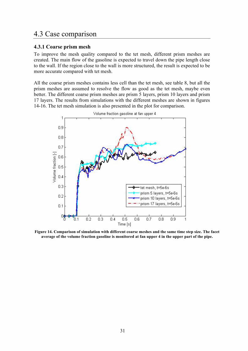
4.3 Case comparison 4.3.1 Coarse prism mesh To improve the mesh quality compared to the tet mesh, different prism meshes are created. The main flow of the gasoline is expected to travel down the pipe length close to the wall. If the region close to the wall is more structured, the result is expected to be more accurate compared with tet mesh. All the coarse prism meshes contains less cell than the tet mesh, see table 8, but all the prism meshes are assumed to resolve the flow as good as the tet mesh, maybe even better. The different coarse prism meshes are prism 5 layers, prism 10 layers and prism 17 layers. The results from simulations with the different meshes are shown in figures 14-16. The tet mesh simulation is also presented in the plot for comparison.

Figure 14. Comparison of simulation with different coarse meshes and the same time step size. The facet

average of the volume fraction gasoline is monitored at fan upper 4 in the upper part of the pipe.

32

Figure 15. Comparison of simulation with different coarse meshes and the same time step size. The facet

average of the volume fraction gasoline is monitored at fan middle 4 in the middle part of the pipe.

Figure 16. Comparison of simulation with different coarse meshes and the same time step size. The facet

average of the volume fraction gasoline is monitored at fan lower 3 in the lower part of the pipe.

The differences between the four cases are not large. It seams like the prism 10 layers and prism 17 layers follow each other and the tet mesh and the prism 5 layers often lies in between, like a average value. The largest difference is for the prism 17 layers in the middle part and in the upper part of the pipe, seen in figures 14-15.

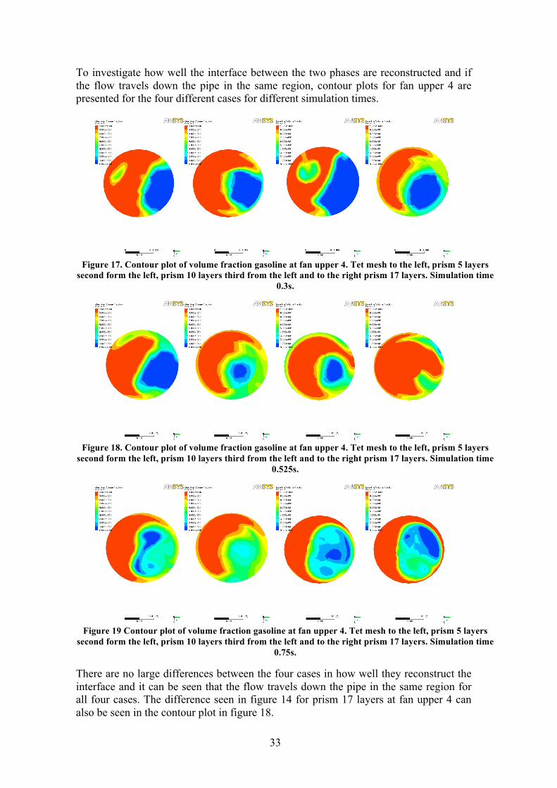
33

To investigate how well the interface between the two phases are reconstructed and if the flow travels down the pipe in the same region, contour plots for fan upper 4 are presented for the four different cases for different simulation times.

Figure 17. Contour plot of volume fraction gasoline at fan upper 4. Tet mesh to the left, prism 5 layers

second form the left, prism 10 layers third from the left and to the right prism 17 layers. Simulation time 0.3s.

Figure 18. Contour plot of volume fraction gasoline at fan upper 4. Tet mesh to the left, prism 5 layers

second form the left, prism 10 layers third from the left and to the right prism 17 layers. Simulation time 0.525s.

Figure 19 Contour plot of volume fraction gasoline at fan upper 4. Tet mesh to the left, prism 5 layers

second form the left, prism 10 layers third from the left and to the right prism 17 layers. Simulation time 0.75s.

There are no large differences between the four cases in how well they reconstruct the interface and it can be seen that the flow travels down the pipe in the same region for all four cases. The difference seen in figure 14 for prism 17 layers at fan upper 4 can also be seen in the contour plot in figure 18.

34

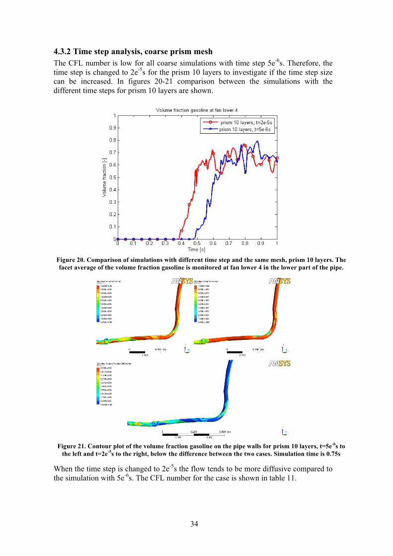
4.3.2 Time step analysis, coarse prism mesh The CFL number is low for all coarse simulations with time step 5e-6s. Therefore, the time step is changed to 2e-5s for the prism 10 layers to investigate if the time step size can be increased. In figures 20-21 comparison between the simulations with the different time steps for prism 10 layers are shown.

Figure 20. Comparison of simulations with different time step and the same mesh, prism 10 layers. The facet average of the volume fraction gasoline is monitored at fan lower 4 in the lower part of the pipe.

Figure 21. Contour plot of the volume fraction gasoline on the pipe walls for prism 10 layers, t=5e-6s to

the left and t=2e-5s to the right, below the difference between the two cases. Simulation time is 0.75s

When the time step is changed to 2e-5s the flow tends to be more diffusive compared to the simulation with 5e-6s. The CFL number for the case is shown in table 11.

35

Table 11. The facet maximum CFL number for different fan surfaces in the upper part of the pipe for prism 10 layers with two different time step after 0.4s simulation time.

Time step 2e-5s, 20 000ts (0.4s)

Time step 5e-6s, 80 000ts (0.4s)

fan surface CFL number CFL number filling pistol inlet 1.41 0.35

upper1 0.8 0.19 upper2 0.61 0.13 upper3 0.79 0.16 upper4 0.44 0.09 upper5 0.43 0.09 upper6 0.44 0.1

middle1 0.44 0.1 middle2 0.41 0.09

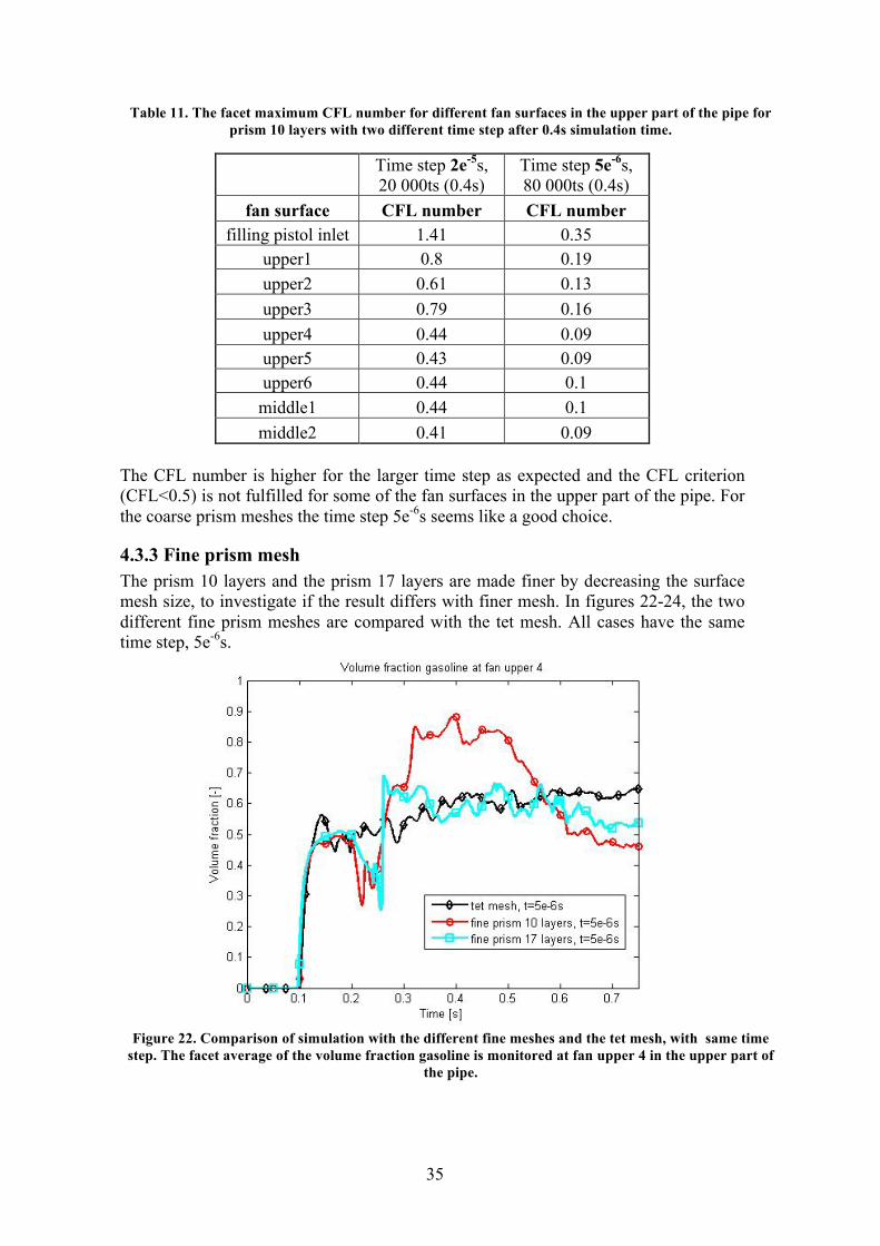
The CFL number is higher for the larger time step as expected and the CFL criterion (CFL<0.5) is not fulfilled for some of the fan surfaces in the upper part of the pipe. For the coarse prism meshes the time step 5e-6s seems like a good choice.

4.3.3 Fine prism mesh The prism 10 layers and the prism 17 layers are made finer by decreasing the surface mesh size, to investigate if the result differs with finer mesh. In figures 22-24, the two different fine prism meshes are compared with the tet mesh. All cases have the same time step, 5e-6s.

Figure 22. Comparison of simulation with the different fine meshes and the tet mesh, with same time

step. The facet average of the volume fraction gasoline is monitored at fan upper 4 in the upper part of the pipe.

36

Figure 23. Comparison of simulation with the different fine meshes and the tet mesh, with same time

step. The facet average of the volume fraction gasoline is monitored at fan middle 4 in the middle part of the pipe.

Figure 24. Comparison of simulation with the different fine meshes and the tet mesh, with same time

step. The facet average of the volume fraction gasoline is monitored at fan lower 3 in the lower part of the pipe.

It seems like the fine meshes resolves the flow situation better than the tet mesh. In the middle and the lower part of the pipe, the two fine meshes follow each other and show similar results. In the upper part of the pipe, a difference can be seen between the fine prism 10 layers and fine prism 17 layers.

37

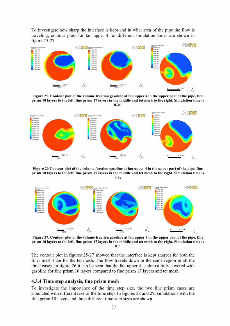
To investigate how sharp the interface is kept and in what area of the pipe the flow is traveling, contour plots for fan upper 4 for different simulation times are shown in figure 25-27.

Figure 25. Contour plot of the volume fraction gasoline at fan upper 4 in the upper part of the pipe, fine prism 10 layers to the left, fine prism 17 layers in the middle and tet mesh to the right. Simulation time is

0.3s.

Figure 26 Contour plot of the volume fraction gasoline at fan upper 4 in the upper part of the pipe, fine prism 10 layers to the left, fine prism 17 layers in the middle and tet mesh to the right. Simulation time is

0.4s

Figure 27. Contour plot of the volume fraction gasoline at fan upper 4 in the upper part of the pipe, fine prism 10 layers to the left, fine prism 17 layers in the middle and tet mesh to the right. Simulation time is

0.7.

The contour plot in figures 25-27 showed that the interface is kept sharper for both the finer mesh than for the tet mesh. The flow travels down in the same region in all the three cases. In figure 26 it can be seen that the fan upper 4 is almost fully covered with gasoline for fine prism 10 layers compared to fine prism 17 layers and tet mesh.

4.3.4 Time step analysis, fine prism mesh To investigate the importance of the time step size, the two fine prism cases are simulated with different size of the time step. In figures 28 and 29, simulations with the fine prism 10 layers and three different time step sizes are shown.

38

Figure 28. Comparison of simulation with different time step and the same mesh, fine 10 layers prism. The facet average of the volume fraction gasoline is monitored at fan upper 4 in the upper part of the

pipe.

Figure 29. Comparison of simulation with different time step and the same mesh, fine 10 layers prism. The facet average of the volume fraction gasoline is monitored at fan lower 3 in the lower part of the

pipe.

The diffusive trend for the larger time step and the coarse mesh seen in figures 20-21 can also be seen for the simulation with the finer mesh. It can also be seen in figures 28-29 that there is not much different between the simulation with time step 5e-6s and the simulation with 2.5e-6s. It appears as that the smaller time step (2.5e-6s) captures

39

more of the flow situation than the larger time step (5e-6s), but the difference is not that great. The CFL number for the fan surfaces in the upper part of the pipe is shown in table 12.

Table 12. The facet maximum CFL number in the upper part of the pipe, for fine 10 layers prism with different time step.

t=2e-5s t=5e-6s t=2.5e-6s fan surface CFL number CFL number CFL number

filling pistol inlet 1.44 0.36 0.21 upper1 1.5 0.39 0.196 upper2 1.8 0.38 0.23 upper3 1.7 0.36 0.21 upper4 1.55 0.26 0.19 upper5 1.12 0.26 0.17 upper6 1.3 0.24 0.17

middle1 1.36 0.2 0.18 middle2 0.61 0.08 0.09

The CFL number is high for the simulation with 2e-5s, above 1 for all fan surfaces in the upper part of the pipe. For the other two time steps, the CFL number are below 0.5, which indicates that the solution is stable for the two lower time step sizes and the time step 5e-6s is small enough. The fine prism 17 layers time step dependency is also investigated. The comparison can be seen in figure 30-31.

Figure 30. Comparison of simulation with different time step and the same mesh, fine prism 17 layers. The facet average of the volume fraction gasoline is monitored at fan upper 4 in the upper part of the

pipe.

40

Figure 31. Comparison of simulation with different time step and the same mesh, fine prism 17 layers. The facet average of the volume fraction gasoline is monitored at fan lower 3 in the lower part of the

pipe.

As for the fine prism 10 layers, the differences between the simulation with time steps 2.5e-6s and 5e-6s are small for the fine prism 17 layers. The smaller time step captures more of the flow situation but overall the differences are not that great. The CFL number varies more for the fine prism 17 layers than for the fine prism 10 layers.

Figure 32. Comparison of simulation with different time step and the same mesh, fine prism 17 layers.

The facet maximum CFL number is monitored at fan upper 1 in the upper part of the pipe.

41

Figure 33. Comparison of simulation with different time step and the same mesh, fine prism 17 layers.

The facet maximum CFL number is monitored at fan upper 4 in the upper part of the pipe.

The CFL number for both time steps gets larger in the beginning of the simulation and then settles to a more or less constant value. For both simulations, the CFL number follows the same trend and the CFL number is smaller for the smaller time step as expected. What happens after 0.35s simulation at fan upper 4 for the smaller time step goes against the trend and the CFL number becomes larger for the smaller time step. The reason for that could be that during simulation with the lower time step a sudden acceleration is captured, that the larger time step misses hence the CFL number becomes larger. To investigate the high CFL number during the beginning of the simulation at fan upper 1, see figure 32, different contour plots for fan upper 1 are shown in figure 34-36.

Figure 34. Contour plots of the CFL number on fan upper 1 for fine prism 17 layers. Left picture is the

triangulated prism mesh and the right is the prism mesh. Simulation time 0.175s.

42

Figure 35. The fan upper 1´s mesh. The triangulated prism mesh to the left and to the right the prism

mesh.

Figure 36. Contour plots on fan upper 1 for fine prism 17 layers, the left picture, volume fraction

gasoline and the right velocity magnitude. Simulation time 0.175s.

In figure 34 the CFL number for fan upper 1 is shown. To the left the triangulated prism mesh and to the right the prism mesh, the two different meshes can be seen in figure 35. It can be seen that the high CFL number is in the triangulated prism mesh region and the CFL number is lower in the prism region. In figure 36 it can be seen that the velocity is very high in the region with the high CFL number and that the gasoline is not present in the area with the high CFL number.

Figure 37. Contour plots for fan upper 4, fine 17 layers prism mesh. The left picture the CFL number, in

middle the velocity magnitude and to the right volume fraction gasoline. Simulation time 0.15s.

The other fan surface with high CFL number is the fan upper 4, see figure 33. In figure 37, the high CFL number is limited to a very small part of the surface (left picture), the region with highest CFL number also have the highest velocity (middle picture) and there is no gasoline present in the region with high CFL number (the right picture). To further investigate the importance of the time step size, the two fine meshes are compared when the smaller time step is used, 2.5e-6s.

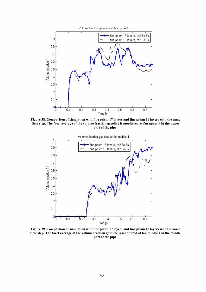
43

Figure 38. Comparison of simulation with fine prism 17 layers and fine prism 10 layers with the same time step. The facet average of the volume fraction gasoline is monitored at fan upper 4 in the upper

part of the pipe.

Figure 39. Comparison of simulation with fine prism 17 layers and fine prism 10 layers with the same time step. The facet average of the volume fraction gasoline is monitored at fan middle 4 in the middle

part of the pipe.

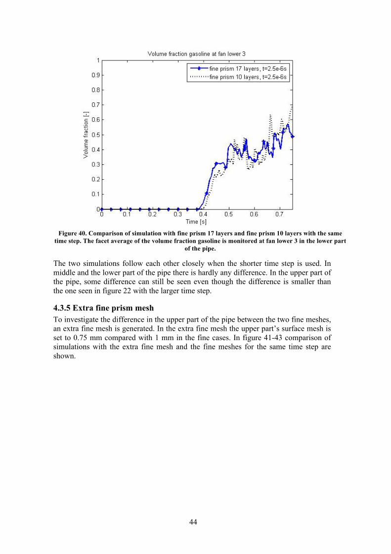
44

Figure 40. Comparison of simulation with fine prism 17 layers and fine prism 10 layers with the same

time step. The facet average of the volume fraction gasoline is monitored at fan lower 3 in the lower part of the pipe.

The two simulations follow each other closely when the shorter time step is used. In middle and the lower part of the pipe there is hardly any difference. In the upper part of the pipe, some difference can still be seen even though the difference is smaller than the one seen in figure 22 with the larger time step.

4.3.5 Extra fine prism mesh To investigate the difference in the upper part of the pipe between the two fine meshes, an extra fine mesh is generated. In the extra fine mesh the upper part’s surface mesh is set to 0.75 mm compared with 1 mm in the fine cases. In figure 41-43 comparison of simulations with the extra fine mesh and the fine meshes for the same time step are shown.

45

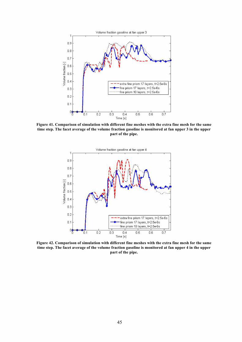
Figure 41. Comparison of simulation with different fine meshes with the extra fine mesh for the same time step. The facet average of the volume fraction gasoline is monitored at fan upper 3 in the upper

part of the pipe.

Figure 42. Comparison of simulation with different fine meshes with the extra fine mesh for the same time step. The facet average of the volume fraction gasoline is monitored at fan upper 4 in the upper

part of the pipe.

46

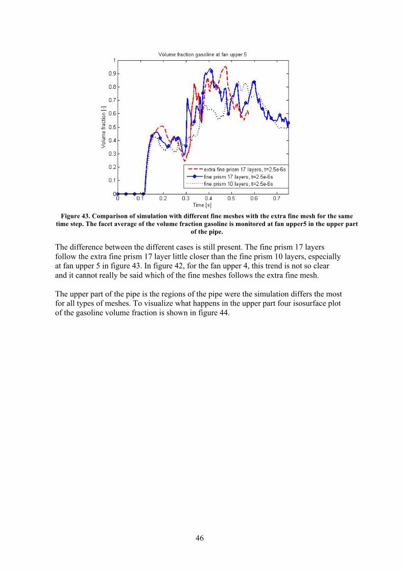
Figure 43. Comparison of simulation with different fine meshes with the extra fine mesh for the same

time step. The facet average of the volume fraction gasoline is monitored at fan upper5 in the upper part of the pipe.

The difference between the different cases is still present. The fine prism 17 layers follow the extra fine prism 17 layer little closer than the fine prism 10 layers, especially at fan upper 5 in figure 43. In figure 42, for the fan upper 4, this trend is not so clear and it cannot really be said which of the fine meshes follows the extra fine mesh. The upper part of the pipe is the regions of the pipe were the simulation differs the most for all types of meshes. To visualize what happens in the upper part four isosurface plot of the gasoline volume fraction is shown in figure 44.

47

Figure 44. Isosurface plots of the volume fraction gasoline in the upper part of the pipe at different simulation times. Upper left 0.1s, upper right 0.2s, lower left 0.3s and lower right 0.4s.

The gasoline injected in the upper part of the pipe is like a jet. It impinging against the wall in the first bend, this is where fan upper 4 is located. After the bend the flow becomes turbulent and continues down the pipe close to the wall. It is the breaking up of the jet that causes the different simulation result for the upper part of the pipe. This is a very difficult region to resolve and maybe another turbulence model or different wall function is needed in this region.

48

4.3.6 Time step analysis, extra fine prism mesh The CFL number for the fan surfaces in the upper part of the pipe for the simulation with the extra fine prism 17 layers mesh and time step 2.5e-6s after 0.3s simulation.

Table 13. The facet maximum CFL number for different fans in the upper part of the pipe after 0.3s simulation. Extra fine pirsm 17 layers with time step 2.5e-6s

t=2.5e-6s, 60 000ts (0.3s) fan surface CFL number filling pistol inlet 0.23 upper1 0.464 upper2 0.475 upper3 0.25 upper4 0.36 upper5 0.11 upper6 0.31 middle1 0.04 middle2 0.04

The CFL number is lower than 0.5 for all the fan surfaces in the upper part of the pipe at 0.3s simulation time. This indicates that the time step is not too large.

4.3.7 Numerical Scheme All the previous presented result has been simulated with first order upwind for the turbulence kinetic energy (k) and dissipation (ε). The first order upwind is known to be more robust than the second order upwind but tends to overestimate the diffusion. The fine 17 layers prism mesh is chosen for investigation of how the numerical scheme affects the result.

Figure 45. Comparison of simulation with different numerical scheme for the fine prism 17 layers mesh and the same time step. The facet average of the volume fraction gasoline is monitored at fan upper 4 in

the upper part of the pipe.

49

Figure 46. Comparison of simulation with different numerical scheme for the fine prism 17 layers mesh

and the same time step. The facet average of the volume fraction gasoline is monitored at fan middle 4 in the middle part of the pipe.

Figure 47. Comparison of simulation with different numerical scheme for the fine prism 17 layers mesh and the same time step. The facet average of the volume fraction gasoline is monitored at fan lower 3 in

the lower part of the pipe.

The figures 45-47 show that there are some differences between the choice of numerical scheme, special in the lower and the middle part of the filling pipe. At the upper part there is almost no difference between the two cases. To further investigate the importance of the numerical scheme and what happens in the middle and lower part of the pipe, an isosurface plot for the middle part of the pipe is shown in figures 48.

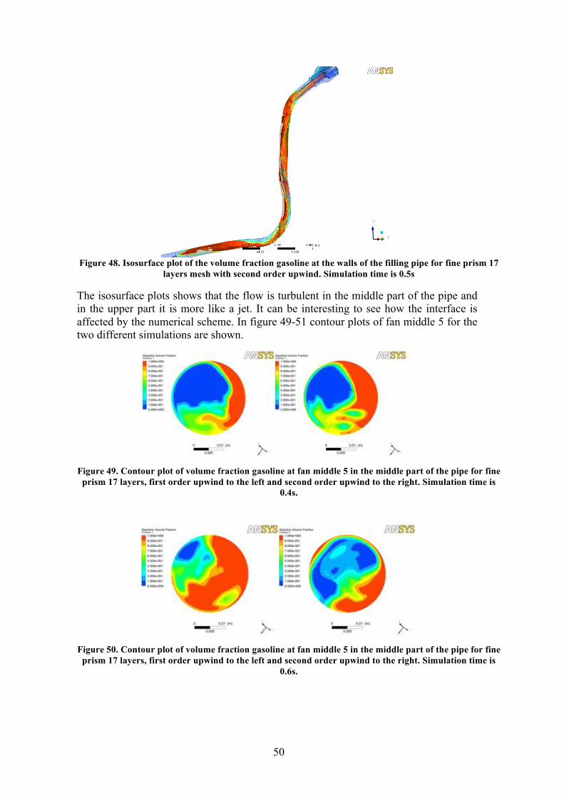
50

Figure 48. Isosurface plot of the volume fraction gasoline at the walls of the filling pipe for fine prism 17

layers mesh with second order upwind. Simulation time is 0.5s

The isosurface plots shows that the flow is turbulent in the middle part of the pipe and in the upper part it is more like a jet. It can be interesting to see how the interface is affected by the numerical scheme. In figure 49-51 contour plots of fan middle 5 for the two different simulations are shown.

Figure 49. Contour plot of volume fraction gasoline at fan middle 5 in the middle part of the pipe for fine

prism 17 layers, first order upwind to the left and second order upwind to the right. Simulation time is 0.4s.

Figure 50. Contour plot of volume fraction gasoline at fan middle 5 in the middle part of the pipe for fine

prism 17 layers, first order upwind to the left and second order upwind to the right. Simulation time is 0.6s.

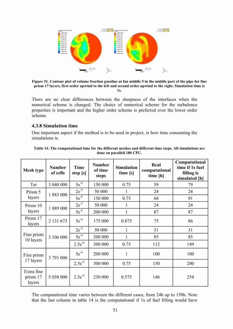
51

Figure 51. Contour plot of volume fraction gasoline at fan middle 5 in the middle part of the pipe for fine

prism 17 layers, first order upwind to the left and second order upwind to the right. Simulation time is 1s.

There are no clear differences between the sharpness of the interfaces when the numerical scheme is changed. The choice of numerical scheme for the turbulence properties is important and the higher order scheme is preferred over the lower order scheme.

4.3.8 Simulation time One important aspect if the method is to be used in project, is how time consuming the simulations is.

Table 14. The computational time for the different meshes and different time steps. All simulations are done on parallell 180 CPU.

Mesh type Number of cells

Time step [s]

Number of time steps

Simulation time [s]

Real computational

time [h]

Computational time if 1s fuel

filling is simulated [h]

Tet 3 040 000 5e-6 150 000 0.75 59 79 2e-5 50 000 1 24 24 Prism 5

layers 1 883 000 5e-6 150 000 0.75 68 91 2e-5 50 000 1 24 24 Prism 10

layers 1 889 000 5e-6 200 000 1 87 87

Prism 17 layers 2 131 673 5e-6 175 000 0.875 75 86

2e-5 50 000 1 31 31 5e-6 200 000 1 85 85 Fine prism

10 layers 3 106 000 2.5e-6 300 000 0.75 112 149

5e-6 200 000 1 100 100 Fine prism 17 layers 3 791 000

2.5e-6 300 000 0.75 150 200

Extra fine prism 17

layers 5 038 000 2.5e-6 230 000 0.575 146 254

The computational time varies between the different cases, from 24h up to 150h. Note that the last column in table 14 is the computational if 1s of fuel filling would have

52

been simulated. It can be seen in the column, that for the finest mesh and the shortest time step, the computational time is 254h. The computational time for the coarse prism meshes and the fine prism meshes is almost the same when the time step 5e-6s is used. This indicates that the size of the time step is more important than the size of the mesh for the computational time.

4.3.9 Hex mesh The simulation with the hexahedron mesh is compared with the fine prism 17 layers mesh for the same time step, 5e-6s.

Figure 52. Comparison of simulation with hex mesh with fine prism 17 layers mesh for the same time

step. The facet average of the volume fraction gasoline is monitored at fan upper 4 in the upper part of the pipe.

Figure 53. Comparison of simulation with hex mesh with fine prism 17 layers mesh for the same time

step. The facet average of the volume fraction gasoline is monitored at fan middle 4 in the middle part of the pipe.

53

Figure 54. Comparison of simulation with hex mesh with fine prism 17 layers mesh for the same time step. The facet average of the volume fraction gasoline is monitored at fan lower 1 in the lower part of

the pipe.

If the result from the simulation with the hex mesh is compared with the fine prism 17 mesh it can be seen that the hex mesh do not captures much of the physics during the simulation and can be assumed to be to coarse. Due to lack of time, further investigation of the hex mesh is not done.

54

5. DISCUSSION

5.1 Mesh A tet mesh is very easy to generate in TGrid, the easiest mesh created during the project. The tet mesh is known to have problem with numerical diffusion since the cells is not aligned with the flow, hence the interface is not kept as sharp as for the finer prism mesh. The prism mesh is expected to give a more structured result with fewer cells than a tet mesh. The procedure in creating a prism mesh is little more time consuming and difficult, but overall not too complicated. A problem with the prism mesh is the first tetrahedral cells growing out from the prism layer. These cells tend to be much smaller and of lower quality than rest of the tetrahedral cells. The problem with smaller cells is that the CFL number can become too high in these cells and cause stability problem during the simulations. Another problem area with less quality in the mesh is the first fan surface in the upper part of the pipe, fan upper 1. To be able to mesh tetrahedral cells in the capless region from the prism cells, the prism cell must be triangulated in TGrid. These triangulated cells tend to have lower quality and cause problem with high CFL number, especially when the fine prism 17 layers mesh is used. The hex mesh is the most difficult mesh to generate but it is assumed to give the most structured result. The filling pipe geometry is very suitable for hex mesh and it would have been interesting to further investigate this mesh type. The capless mesh is too fine. The capless mesh could be made coarser by changing the growth rate from 1.1 up to 1.6 in TGrid. The capless geometry can also be more simplified to further improve the mesh quality. If the flow situation is studied in the capless, it can be seen that the gasoline injected is more or less a jet, that goes right through the capless and out in the upper part of the pipe. This is also a reason why the geometry can be simplified and a coarser mesh can be applied.

5.2 Explicit vs. implicit VOF The explicit discretization of the volume fraction equation is a more mathematical effective model than the implicit. It is therefore assumed to be more computational effective. Simulations with the explicit VOF could diverged after 22 000 converged time step. The reason for this is not fully understood; perhaps there is some sudden acceleration somewhere in the lower region of the pipe or splashing of fuel causing acceleration of the fluid. But it is known that the explicit VOF is sensitive for too large time steps. Therefore the choice of the time step becomes very crucial for the explicit VOF. Variable time stepping was adopted to avoid problem with too large time step. The variable time stepping algorithm changes the time step according to the global CFL number. But the global CFL number was set too high and a too large time step was used and the simulation diverged.

55

For the implicit VOF, the simulation did not diverged when a too large time step is used. But there were problems with larger residuals for the turbulence properties. Therefore the simulation becomes unstable and unnecessary time consuming. This is why the CFL criterion is used to find a suitable time step for the simulation with the implicit VOF. Due to the lack of stability with the explicit VOF, the implicit VOF should be chosen as discretization scheme for the volume fraction equation during simulation of fuel filling.

5.3 Case comparison The case comparison follows a red thread. The simulation starts with the coarse prism meshes. The mesh is continuously made finer to investigate how the result varies with finer grid until the finest mesh is reached. As the mesh is made finer the time step have to be investigated due to the CFL number.

5.3.1 Coarse prism mesh Simulation with all the coarse prism meshes shows similar results as simulation with the tet mesh for the same time step. Comparison between the three different coarse prism meshes showed little difference. The mesh size is about the same for prism 5 layers and prism 10 layers. The prism 17 layers mesh is the most dense coarse prism mesh. It can be assumed that this mesh would give the most accurate result. The prism 10 layers follow the prism 17 layers more closely than the prism 5 layers. The prism 5 layers follow the tet mesh more than the prism 17 layers and it’s most likely a poorer choice of mesh. The prism 5 layers are not chosen for further investigation.

5.3.2 Time step, coarse prism mesh The simulation with the larger time step size (2e-5s) and prism 10 layers mesh is more diffusive than the simulation with the same mesh and the time step 5e-6s. The CFL number is also larger, and the CFL criterion is not fulfilled for some of the fan surfaces in the upper part of the pipe. This indicates that the time step 5e-6s is a good choice for the prism 10 layers. The time step dependence for the prism 17 layers is not investigated.

5.3.3 Fine prism mesh When the simulations with the finer prism meshes are compared with the tet mesh, a large difference can clearly be seen. The mesh size for the fine prism 10 layers is in the same magnitude as the tet mesh, but the fine prism 10 layers capture more of the flow situation than the tet mesh. The expected diffusive property of the tet mesh is clearly seen here and the prism mesh is a much better choice for this kind of simulation. This is also seen in the contour plots over fan upper 4. The interface is kept sharper for the fine prism meshes than for the tet mesh. The difference between the fine meshes is mostly in the upper part of the pipe. In the lower and the middle part of pipe the simulation results are similar. The difference in the upper part of the pipe is discussed in chapter 5.3.5 Extra fine mesh.

56

5.3.4 Time step, fine prism mesh The CFL number is below 0.5 for all the fan surfaces in the upper part of the pipe for fine 10 layers prism. It is therefore of interest to investigate if the time step could be set higher to save computational time. The simulation showed that the larger time step, 2e-5 is too large and the simulation showed the same diffusive trend as for the prism 10 layers. The smaller time step showed the same trend for both the finer meshes. Simulation with the smaller time step, a little more of the flow situation is captured. This is because the flow stays longer in every cell hence there is more time to capture more of the flow situation within the cell. But the simulation becomes more time consuming with the smaller time step. The small difference between the two time steps are acceptable and it is assumed that the time step 5e-6s is the best choice. The CFL analysis for the fine prism 17 layers showed that the CFL number is above 0.5 for both time steps (5e-6s and 2.5e-6s) at fan upper 1 and fan upper 4. The high CFL number for fan upper 1 is in the triangulated prism cells. It can be seen that the area with high CFL number is where there is no gasoline present. The high CFL number can be accepted as long as the simulations converge. The same goes for the high CFL number at fan upper 4. There it is in the smaller tetrahedral cells growing out from the prism layer that causes problems. In the region with high CFL number there is no gasoline present hence it can be accepted as long there are no problem with the simulations. The difference between the simulation with the smaller time step (2.5e-6s) and the fine prism meshes showed almost no difference in the lower and middle part of the pipe. But in the upper part there is still a difference between the two simulations. The difference is smaller than for the time step 5e-6s but still there are some differences. The extra fine prism mesh is created to further investigate the upper part of the pipe.

5.3.5 Extra fine prism mesh It is assumed that the upper part of the filling pipe is the region that can cause the most problem during fuel filling. It is also the region were the result from the prism meshes varies the most. The comparison between the extra fine prism mesh and the fine prism mesh indicates that the fine prism 17 layers follows the extra fine mesh better than the fine prism 10 layers but there are still some differences between the simulations. The contour plots can explain why the result from simulations of the upper pipe, especially at fan upper 4, has varied throughout the entire project. The gasoline comes in as a jet in the upper part and impinging against the wall. This happens almost exactly at fan upper 4. This flow situation appears to be difficult to simulate. Maybe it can be the choice of turbulence model that affect the results. The realizable k-ε is known to handle swirling flows, flow separation and round jets better that the standard k-ε but maybe k-ω can handle the wall region better. Or maybe it is the use of the standard wall function that causes the problem. The standard wall function is known to have problem in handling impinging flows and a non-equilibrium wall function might have been a better choice.

57

5.3.6 Numerical scheme In the beginning of the project there were problems with convergence during the simulations, the residual for the turbulence properties where the ones that diverged. Therefore the numerical scheme was changed from second order upwind to first order upwind for k and ε. The change of numerical scheme did not affect the flow in the upper part of the pipe. This is because the flow is not that turbulent in the upper part. The flow is more like a jet through the region and it is first after it struck the first bend it start to be become more turbulent. In the middle and lower part of the pipe the difference between the simulations with the different numerical schemes are more obvious. The flow is more turbulent here and the second order upwind will be less diffusive than the first order upwind. However, the sharpness of the interface is not affected by the numerical scheme as it might have been expected. The volume of fluid is a first order accurate model and the interface is more affected by the size of the mesh than the order of turbulence discretization scheme.

5.3.7 Simulation time The transient simulation with volume of fluid can be very time consuming. It depends on the number of cells, the size of the cells and the transient time step size. In this project, it is estimated that at least 0.75-1s of fuel filling needs to be simulated to ensure that the flow reaches the outlet. When the same time step is used, the computational time between the coarse prism meshes, the fine prism meshes and the tet mesh is in the same magnitude, between 80-100h for 1s simulation. But if the time step size is made smaller the computational time becomes much larger, 150-250h. Keeping the time step large is more important for shorter computational time than the sizes of the mesh. The problem is that if the mesh size is smaller then the time step must also be smaller to fulfill the CFL criterion (CFL<0.5), hence if a fine mesh is used, the time step must be kept small.

5.3.8 Hex mesh Unfortunately the mesh created was too coarse, the pipe only consist of 150 000 cells. Even though the few cells, the simulation with the hex mesh showed similar results as the tet mesh, it acted as an average of the finer prism mesh. This mesh type is recommended for future investigations.

58

6. CONCLUSION AND RECOMMENDATION The simulation results presented in this reports indicates that there are great possibilities in simulation of fuel filling with volume of fluid. The computational time is acceptable and the result looks promising. The implicit VOF is a more stable discretization method than the explicit VOF. It is not so sensitive to high CFL numbers and it is not too computational expensive. All the prism mesh showed similar or better result than the previous used tet mesh. Since there are no experiments to verify the simulations with, recommendation of a mesh is impossible. The level of information needed is not known, meaning how well the flow needs to be resolved for an accurate enough prediction of fuel filling. The experiments are also necessary to verify if the tank needs to be present during the simulation or not. The recommendations from this project are based on the comparison of the different cases. The most promising method from this comparison is the fine prism 17 layers mesh with time step 5e-6s and second order upwind scheme for the turbulence properties. It captures more of the flow than the coarse prism meshes and tet mesh and follows the extra fine mesh better in the upper part than the fine prism 10 layers. The computational time for this mesh is acceptable and the time step used is proven to be in the right magnitude. The hex mesh could be interesting to investigate further. It is really structured and should work fine to predict fuel filling. The mesh is not necessary created in Ansa, it might be created in Harpoon with the same good result. To improve the handling of the upper region of the pipe, non-equilibrium wall function can be tested. The standard wall function is known to have problem with impinging flow.

REFERENCES 1. Andersson. B., Andersson. R., Håkansson. L., Mortensen. M., Sudiyo. R. and

van Wachem. B. (2010) Computational Fluid Dynamics for Chemical Engineers. 6-th edition. Gothenburg. Sweden

2. Clift. R., Grace. J. R. and Weber. M. E. (1978) Bubbles, Drops and Particles. London: Academic Press INC LTD.

3. Hirt. C. W. and Nichols B. D. (1979) Volume of Fluid (VOF) Method for the Dynamic of Free Boundaries. Journal of computational physics. (1981). vol 39. page 201-225.

4. Dang Hieu. P. and Tanimoto. K. (2006) Verification of a VOF-based two-phase flow model for wave breaking and wave-structure. Ocean Engineering 33. page 1565-1588. www.elsevier.com/locate/oceaneng [2011-01-21]

5. Ansys Fluent. v13 Documentation. – Southpointe : Software guide –bundled with Ansys Fluent v13 [2011-05-10]

6. Barton. I. E. (1998) Comparison of SIMPLE- and PISO algorithms for transient flows. International Journal for numerical methods in fluids, vol. 26. page 459-483 [2011-03-22]

7. Courant. R., Friedrichs. K and Lewy. H. (1967) On the Partial Difference Equations of Mathematical Physics. IBM Journal. p.p 215-234 http://www.stanford.edu/class/cme324/classics/courant-friedrichs-lewy.pdf [2011-05-03]

8. BETA CAE Systems S. A. (2010) Ansa. http://www.beta-cae.gr/ansa.htm [2011-01-24].

9. ANSYS (2011) TGrid. http://www.ansys.com/Products/Other+Products/TGrid [2011-01-24]

10. ANSYS (2011) Fluent. http://www.ansys.com/Products/Simulation+Technology/Fluid+Dynamics/ANSYS+FLUENT [2011-05-28]

11. ANSYS (2011) CFD-Post. http://www.ansys.com/Products/Simulation+Technology/Fluid+Dynamics/ANSYS+CFD-Post [2011-05-28]

12. Virdung. T. (2009) CFD of Fuel Filling in Y283, CFD report, Volvo Car Corporation