Numerical Simulation of Complex and Multiphase Flows

Porquerolles, 18-22 April 2005

•thanks to: ERCOFTAC, Conseil Général Var, Région PACA, USTV and Stana.

•copy of the students passports (ERCOFTAC grants).

•extra nights have to be paid today.

•lectures (morning) and advanced communications (afternoon).

Applications of the finite volumes method for complex flows: from the theory to the

practice

Philippe HELLUY,

ISITV, Université de Toulon,

France.

Spring school « numerical simulations of multiphase and complex flows », 18-22 April 2005, Porquerolles.

I) Introduction to finite volumes for hyperbolic systems of conservation laws.

II) An industrial application.

III) Mixtures thermodynamics and numerical schemes for phase transition flows.

IIntroduction to finite volumes for

hyperbolic systems of conservation laws

Example: let u(x,t) be a solution to

Characteristic curve

0.t xu cu

( ( ), ) 0,

'( ) 0.t x

du x t t

dtu x t u

The characteristic has thus the equation '( ) ,

Cst

x t c

x ct

That implies that u is an arbitrary function of x-ct.

A characteristic is a curve along which a regular solution of a first order Partial Differential Equation (PDE) is constant

u(x(t),t)=Cst

Other example: Burgers equation 2 / 2 0t xu u

A regular solution satisfies 0t xu u u

The characteristic equation is thus '( ) ( ( ), )x t u x t t

0 0( ) ( ,0)x t x u x t

Consider now an initial condition of the form

1 if 0,

( ,0) 1 if 0 1,

0 if 1.

x

u x x x

x

If u were regular, it would imply u(x,t)=1=0 if x>1 and t>1

or

Admissible shock waveA shock wave is a discontinuous solution of a first order PDE, wt+f(w)x=0, emerging from an intersection of characteristics.If the shock curve is parametrized by (x(t),t), the normal vector to the shock is n=(1,-s), with s=x’(t).

We denote by [w]=wR -wL the jump of the quantity w in the shock. According to distribution theory, we must have the Rankine-Hugoniot relation

( ) 0,

( ) .

t xn w n f w

s w f w

The characteristic intersection condition gives

'( ) '( ).L Rf w s f w Lax’s condition (for Burgers: uL>uR )

(For Burgers:s=1/2(uL+uR) )

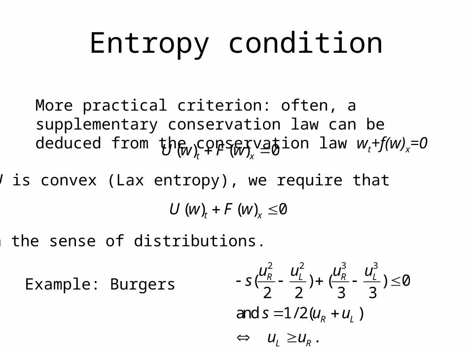
Entropy condition

More practical criterion: often, a supplementary conservation law can be deduced from the conservation law wt+f(w)x=0

( ) ( ) 0t xU w F w

If U is convex (Lax entropy), we require that

( ) ( ) 0t xU w F w

In the sense of distributions.

Example: Burgers2 2 3 3

( ) ( ) 02 2 3 3

and 1/ 2( )

.

R L R L

R L

L R

u u u us

s u u

u u

The Riemann problemExample of the Burgers equation

2( / 2) 0,

, if x<0,( ,0)

if 0.

t x

L

R

u u

uu x

u x

+ entropy condition

The solution is noted R(x/t,uL,uR) and is

if /

( , ) / if /

if /

L L

L R

R R

u x t u

u x t x t u x t u

u u x t

if /( , ) 2

if /

L RL

R

u uu x t

u x tu x t

L Ru uL Ru u

Rarefaction wave Shock wave

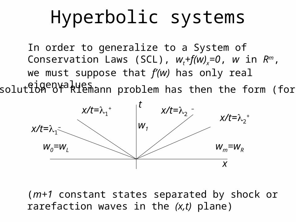
Hyperbolic systems

In order to generalize to a System of Conservation Laws (SCL), wt+f(w)x=0, w in Rm, we must suppose that f’(w) has only real eigenvalues.

The solution of Riemann problem has then the form (for m=2)

x/t=1–

x/t=1+

w0=wL wm=wR

x/t=2+

x/t=2 –

w1

x

t

(m+1 constant states separated by shock or rarefaction waves in the (x,t) plane)

Finite volume schemes

In two dimensions the SCL reads wt+f(w)x+g(w)y=0, and one solves a Riemann problem for each edge between two finite volumes in the normal direction to the edge.

Ci

Cj

1( , ) ( , )

i

ni i n nC

w w x t w x t dxh

11/ 2 1/ 2

1/ 2 1

0,

( (0, , )).

n n n ni i i i

n n ni i i

w w f f

h

f f R w w

Godunov flux

"Exact" in some sense, and satisfies a discrete entropy inequality

In one dimension: let be a time step, h a space step, xi=ih, tn=n, The cell (or finite volume) Ci is the interval ]xi-1/2,xi+1/2[

max/(2 ).h

IIIndustrial application

(Oz)

Conditiond'entrée

Sortie

Parois

Multifluid modelGas generator: industrial tool to eject device

•Two phases (air and water)•Compressible (pressure up to 300 atm)•Duration: 50 ms, thus evaporation and viscosity neglected.

The unknowns are the density (x,t), the velocity u(x,t), the internal energy (x,t) the pressure p(x,t) and the mass fraction of gas y(x,t)Euler equations (in 1D in order to simplify)

2

2 2

( ) 0,

( ) ( ) 0,

( / 2) (( / 2 ) ) 0,

( ) ( ) 0.

t x

t x

t x

t x

u

u u p

u u p u

y uy

Pressure law: ( , , )p p y

2

2 2

( , , / 2, ) ,

( ) ( , ,( / 2 ) , ) .

T

T

w u u y

f w u u p u p u yu

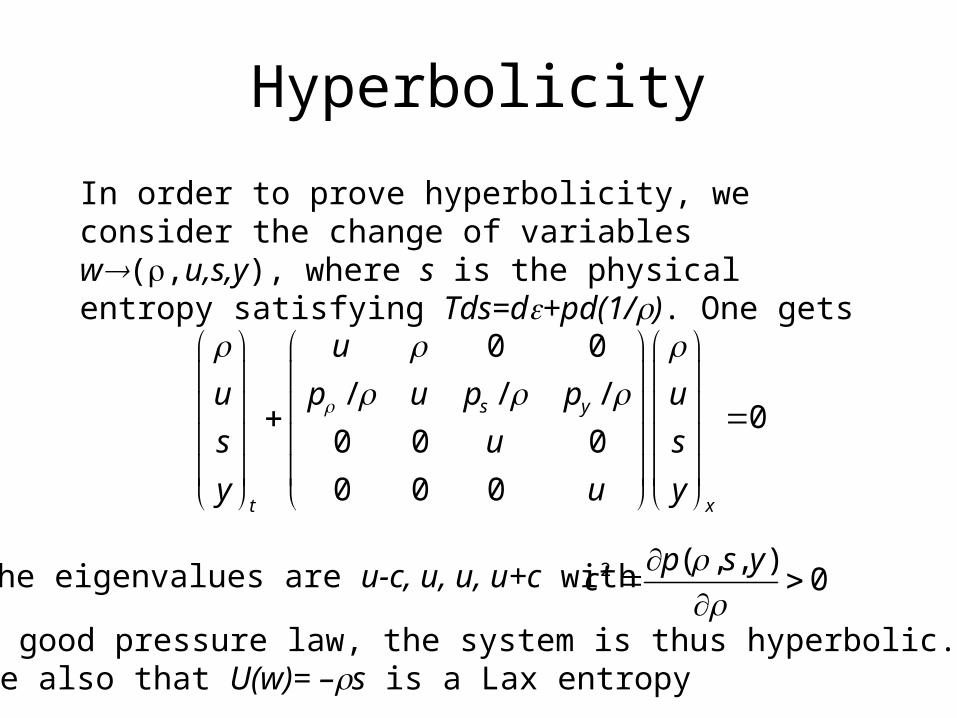
Hyperbolicity

In order to prove hyperbolicity, we consider the change of variables w(,u,s,y), where s is the physical entropy satisfying Tds=d+pd(1/). One gets

0 0

/ / /0

0 0 0

0 0 0

s y

t x

u

u p u p p u

s u s

y u y

The eigenvalues are u-c, u, u, u+c with 2 ( , , )0

p s yc

With a good pressure law, the system is thus hyperbolic.We have also that U(w)= –s is a Lax entropy

Practical pressure lawWe use a pressure law that allows the exact resolution of the Riemann problem and acceptable precision: the stiffened gas equation of state (EOS)

air water

air air water water

air water

( 1) ,

( ), ( ),

1 1 1(1 ) ,

1 1 1

(1 ) .1 1 1

p

y y

y y

y y

For numerical reasons, it appears that the last conservation law should be replaced by a non-conservative transport equation (Abgrall-Saurel 1996)

0.t xy uy

2 .p

c

then

Numerical results

Rouy, 2000

IIIMixtures thermodynamics and numerical schemes for phase

transition flows.

Cavitation

boiling

Demonstration

Liquid area heated at the center by a laser pulse

Bubble collapse near a rigid wall

Ambient liquid (1atm)

Heated liquid (1500 atm)

2.0 mm, 70 cells

2.4 mm, 70 cells

1.4 mm

0.15 mm 0.45 mm

Wall

Mixture pressure (from 0 to 2ns)

Bubble close to a rigid wall

Volume Fraction of Vapor (from 0 to 66ns)

Bubble close to a rigid wall

1) Thermodynamics of a single fluid and of an immiscible mixture of two fluids;2) Relaxation scheme for flow with phase transition (coupling the hydrodynamics and the thermodynamics);3) Miscible mixtures and super-critical fluids.

Mixtures thermodynamics and numerical schemes for phase

transition flows

•T. Barberon and Helluy. Finite volume simulation of cavitating flows. Computers and Fluids, 2004.•P. Helluy, N. Seguin. A simple model for super-critical fluids, 2005, preprint.

Single fluid thermodynamics

S(W) is the entropy. It is extensive and concave

We define the temperature T by1 S

T E

The pressure p byp S

T V

S

T M

The chemical potential

TdS dE pdV dM This gives

Single fluid of mass M, volume V and energy E. W=(M,V,E).

An extensive variable X is a function of W that is Positively Homogeneous of degree 1 (PH1) : X is an intensive variable if it is PH0:

0, ( ) ( ).X W X W

0, ( ) ( ).X W X W

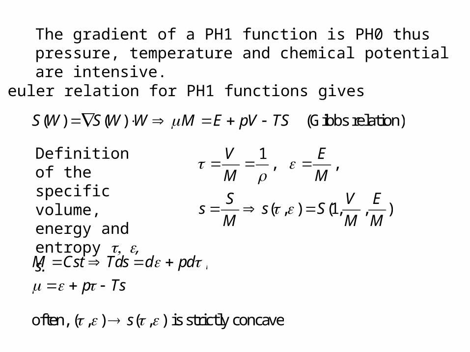
The gradient of a PH1 function is PH0 thus pressure, temperature and chemical potential are intensive.

The euler relation for PH1 functions gives

( ) ( ) (Gibbs relation)S W S W W M E pV TS

Definition of the specific volume, energy and entropy , s.

1, ,

( , ) (1, , )

V E

M M

S V Es s S

M M M

,M Cst Tds d pd

p Ts

often, ( , ) ( , ) is strictly concaves

The sound speed c of the fluid computed from p=p() must be real

2 2/c pp p 2 2 2( 2 ) ( , 1),

quadratic form <0

c T p s ps s TQ p

Q

Hyperbolicity if0,

concave.

T

s

The sign of p is not important…

Hyperbolicity

•H. B. Callen. Thermodynamics and an introduction to thermostatistics, second edition. Wiley and Sons, 1985.•J.-P. Croisille. Contribution à l’étude théorique et à l’approximation par éléments finis du système hyperbolique de la dynamique des gaz multidimensionnelle et multiespèces. PhD thesis, Université Paris VI, 1991.

Mixture of two immiscible fluids (1) and (2)

1 1 1 1 2 2 2 2( , , ), ( , , )W M V E W M V E

Mixture entropy out of equilibrium

1 2 1 1 2 2( , ) ( ) ( )S W W S W S W

1 2 and entropies of the two fluidsS S

Constraints 1 2 1 2 1 2( , ), , 0,Q W W W W W W W

Equilibrium entropy1 2

1 2( , )

( ) max ( , )W W Q

S W S W W

at equilibrium: 1 2 1 2 1 2, and .T T p p (Isobaric law)

M1,V1,E1

M2,V2,E2

M,V,E

1 2

1 1( , , ) ( , ) (1 ) ( , )

1 1

z zs Y s s

out-of-equilibrium pressure and temperature:1

,

thus ( , , ) and ( , , ).

s p s

T Tp p Y T T Y

It is more practical to use intensive variables.

1

1

1

volume fraction ,

mass fraction ,

energy fraction .

V

VM

ME

zE

1 2( , )out-of-equilibrium specific entropy: ( , , )

S W Ws Y

M

fractions vector ( , , )Y z

Out-of-equilibrium specific entropy

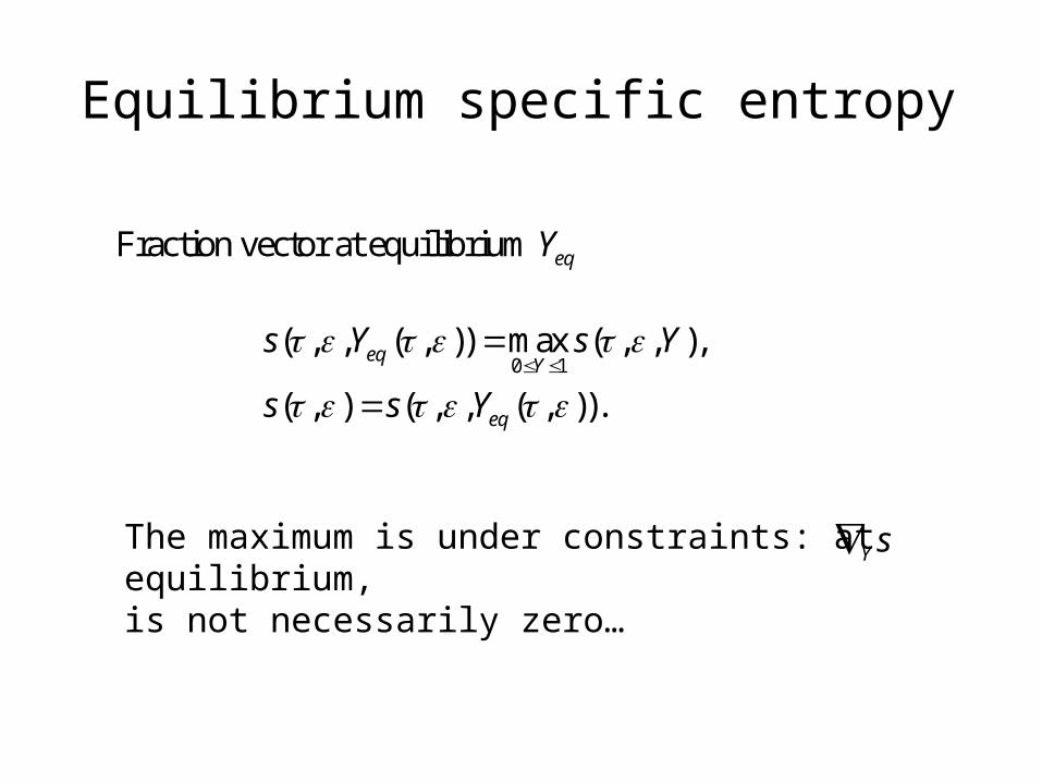
Equilibrium specific entropy

0 1( , , ( , )) max ( , , ),

( , ) ( , , ( , )).

eqY

eq

s Y s Y

s s Y

Fraction vector at equilibrium eqY

The maximum is under constraints: at equilibrium, is not necessarily zero…

Y s

Simple example (perfect gases mixture)

The fractions and z can then be eliminated.

1with ln( ).ii i is

We suppose temperature and pressure equilibrium

0.s s

z

1 1

2 2

1 2

ln ( 1) ln ( 1) ln( 1)

(1 )( 1) ln( 1) ( 1) ln( 1),

( ) (1 ) .

s

Out-of-equilibrium specific entropy (before mass transfer)

1 2

1 1( , , ) ( , ) (1 ) ( , )

1 1

z zs Y s s

Pressure law out of equilibrium and saturation curve

Out of equilibrium, we have a perfect gas law

The saturation curve is thus a line in the (T,p) plane.

On the other side,1 2

1 1 2 2

( ) ln1

( 1)(ln( 1) 1) ( 1)(ln( 1) 1).

s

1 1,

( ) 1( 1) ,

( ( ) 1) .

s

Ts p

pT

p

0 Cste1

s T

p

Phase 2 is the most stable Phase 1 is the most stable

Phases 1 and 2 are at equilibrium

Optimization with constraints of ( , , )

(here, ), ( , ) being fixed.

s Y

Y

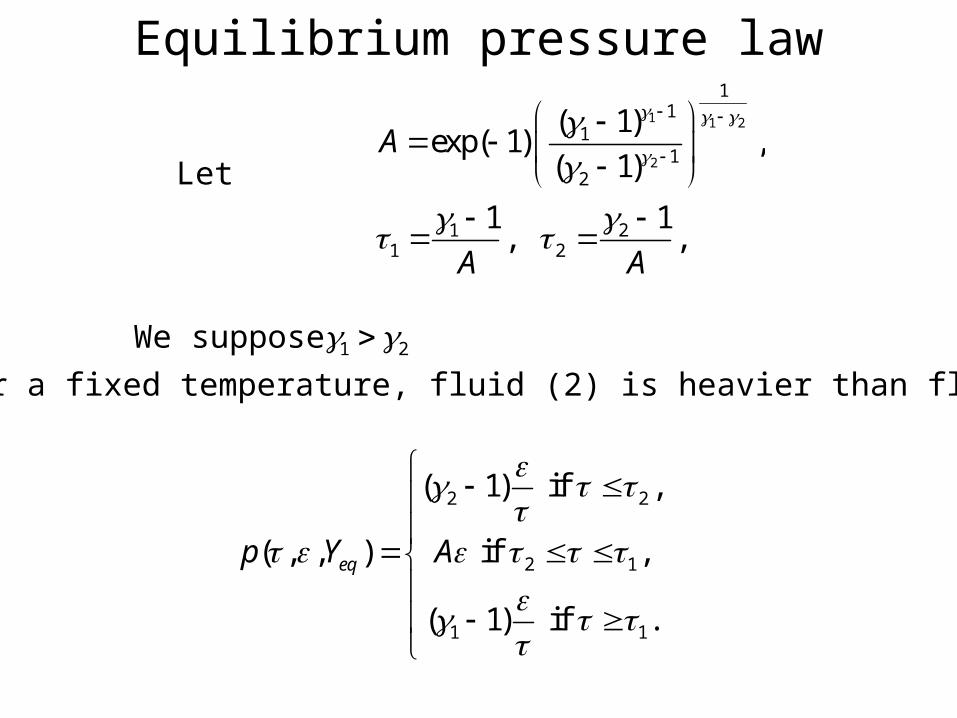
Equilibrium pressure law

Let

We suppose

(for a fixed temperature, fluid (2) is heavier than fluid (1))

2 2

2 1

1 1

( 1) if ,

( , , ) if ,

( 1) if .

eqp Y A

1 1 2

2

11

11

2

1 21 2

( 1)exp( 1) ,

( 1)

1 1, ,

A

A A

1 2.

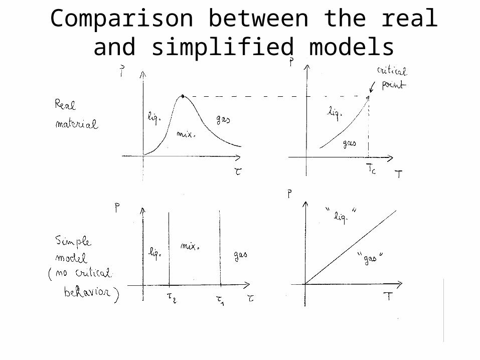
Comparison between the real and simplified models

Partial conclusion:•the temperature and pressure of the mixture are obtained from the entropy;•the equilibrium entropy is solution of a constrained convex optimisation problem.

Next step:•coupling with hydrodynamics;•numerical scheme.

One-velocity two-fluid models

2

2 2

( ) 0,

( ) ( ) 0,

( / 2) (( / 2 ) ) 0,

( ).

t x

t x

t x

t x eq

u

u u p

u u p u

Y uY Y Y

0 1

is computed from the out-of-equilibrium entropy

is the equilibrium fractions vector:

( , , ) max ( , , ).

eq

eqY

p

Y

s Y s Y

positive matrix

0 0

= 0 0

0 0

0 0 0

= 0 0

0 0

Instantaneous equilibrium No phase transition

Y

z

Other possible models…

Formal limit +

2

2 2

( ) 0,

( ) ( ) 0,

( / 2) (( / 2 ) ) 0,

( , , ).

t x

t x

t x

eq

u

u u p

u u p u

p p Y

It is natural to study the weak entropy solutions of the formal limit system:

•R. Menikoff and B. J. Plohr. The Riemann problem for fluid flow of real materials. Rev. Modern Phys., 61(1):75–130, 1989. •S. Jaouen. Étude mathématique et numérique de stabilité pour des modèles hydrodynamiques avec transition de phase. PhD thesis, Université Paris VI, November 2001.

•Generally, this system has several Lax solutions•Liu entropy criterion is more adequate

Standard schemes as Rusanov's may converge towards different solutions

CFL=0.9418 CFL=0.9419

density

numerical entropy production

Relaxation scheme based on entropy optimisation

When =0, the previous system can be written in the classical form

2

2 2

( ) 0,

( , , ( / 2), ) ,

( ) ( , , ( ( / 2) ) , )

t x

T T

T T

w f w

w u u Y

f w u u p u p u uY

1) Finite volumes scheme (relaxation of the pressure law)

1/ 21/ 2 1/ 2

1/ 2 1

( , ),

0,

( , ) Godunov flux (computable)

ni

n n n ni i i i

n n ni i i

w w n t i x

w w F F

t x

F F w w

2) Projection on the equilibrium pressure law1 1/ 2 1 1/ 2 1 1/ 2, ,n n n n n n

i i i i i iu u 1 1 1 1 1

0 1( , , ) max ( , , )n n n n n

i i i i iY

s Y s Y

Other works about relaxation schemes

• Yann Brenier. Averaged multivalued solutions for scalar conservation laws. SIAM J. Numer. Anal., 1984.• B. Perthame. Boltzmann type schemes for gas dynamics and the entropy property. SIAM J. Numer. Anal., 1990. • F. Coquel and B. Perthame. Relaxation of energy and approximate Riemann solvers for general pressure laws in fluid dynamics. SIAM J. Numer. Anal., 1998.• Saurel, Richard; Abgrall, Rémi A multiphase Godunov method for compressible multifluid and multiphase flows. J. Comput. Phys., 1999.• G. Chanteperdrix, P. Villedieu, and Vila J.-P. A compressible model for separated two-phase flows computations. In ASME Fluids Engineering Division Summer Meeting. ASME, Montreal, Canada, July 2002. • Stéphane Dellacherie. Relaxation schemes for the multicomponent Euler system. M2AN Math. Model. Numer. Anal., 2003.•…

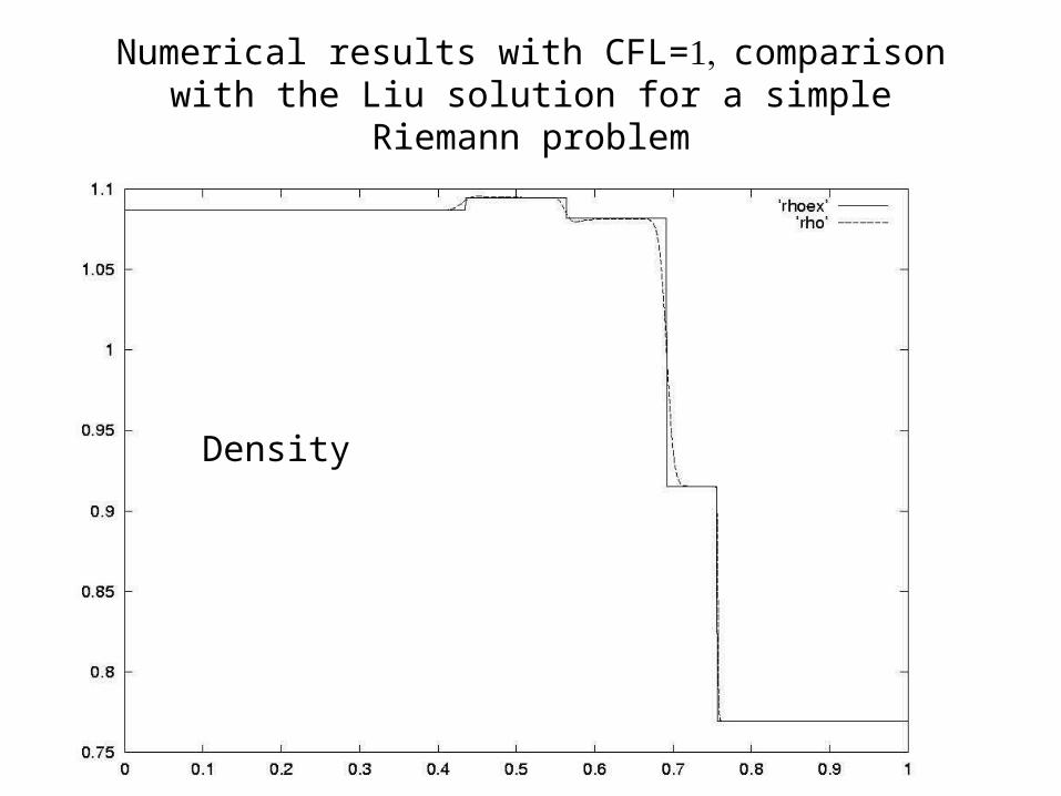
Numerical results with CFL=comparison with the Liu solution for a simple Riemann problem

Density

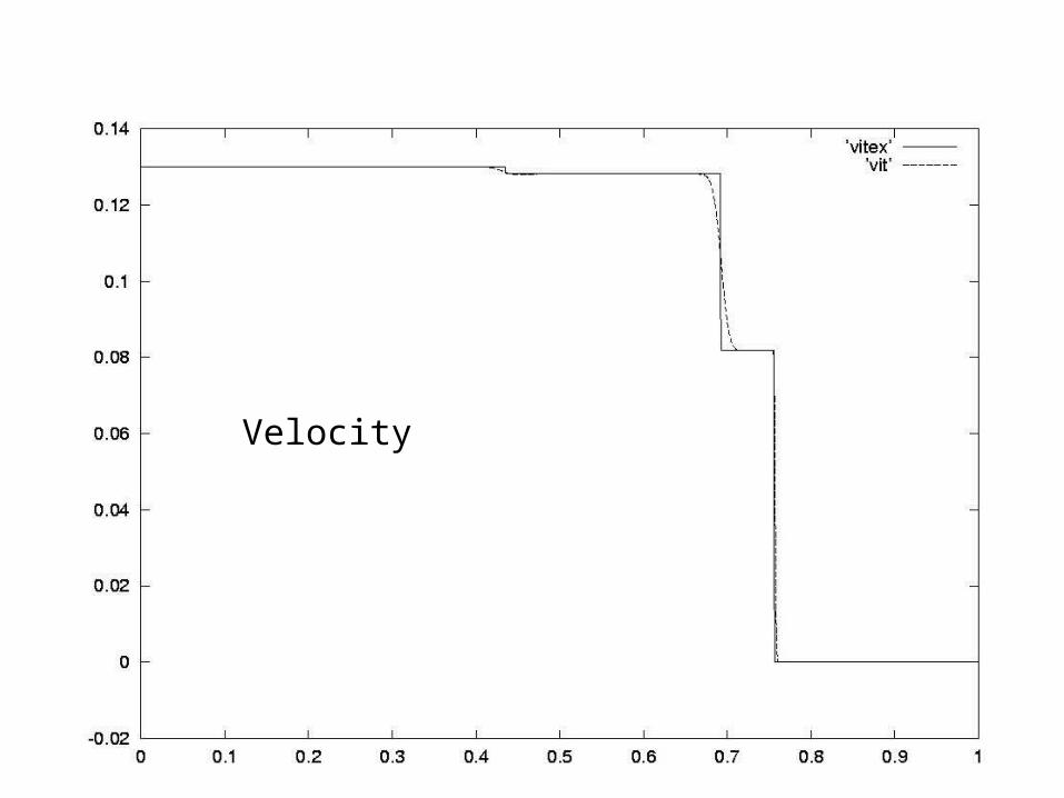
Velocity

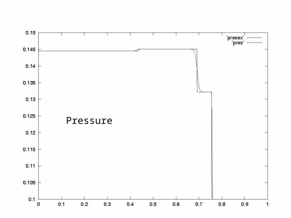
Pressure

Mixture of stiffened gases

1 0Stiffened gas entropy: ln(( )ii i i i is C Q s

•We suppose only temperature equilibrium (elimination of z).•Out of equilibrium, the mixture still satisfies a stiffened gas law: exact Riemann solver in the relaxation step.•Equilibrium is obtained after optimization with respect to and .•The pressure law is not analytic.

0Coefficients , , , , , 1, 2, are fitted to experimentsi i i i iC Q s i

Liquid area heated at the center by a laser pulse

Bubble collapse near a rigid wall

Ambient liquid (1atm)

Heated liquid (1500 atm)

2.0 mm, 70 cells

2.4 mm, 70 cells

1.4 mm

0.15 mm 0.45 mm

Wall

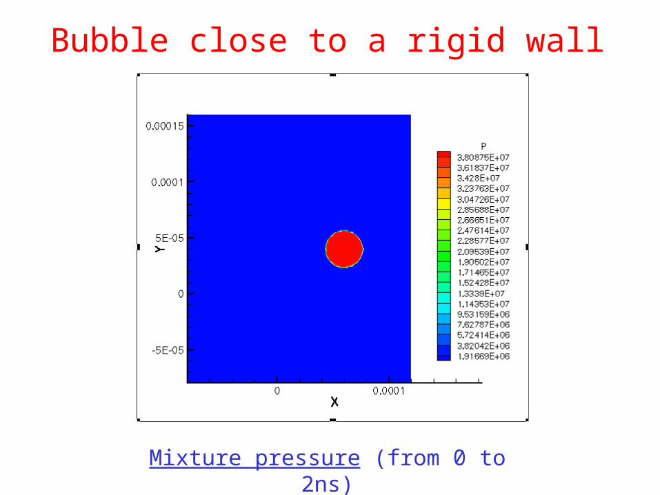
Mixture pressure (from 0 to 2ns)

Bubble close to a rigid wall

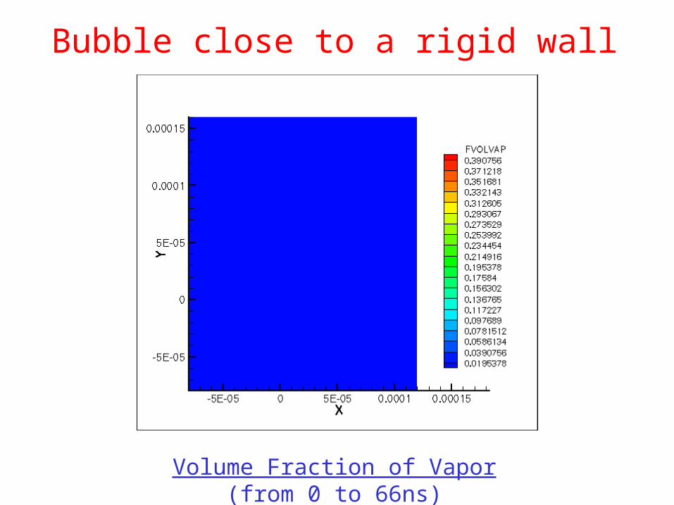
Volume Fraction of Vapor (from 0 to 66ns)

Bubble close to a rigid wall

Partial conclusion:•the relaxation scheme is based on entropy optimisation•it seems to converge towards the Liu solution•it can be used in practical configurations

Next step: super-critical fluids

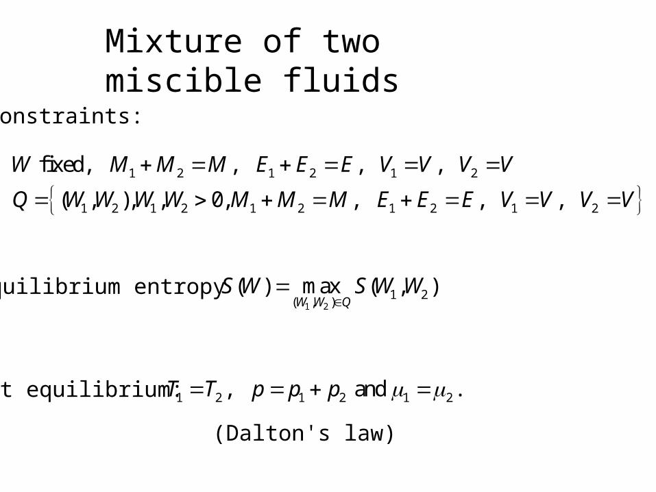
Mixture of two miscible fluids

Constraints:

1 2 1 2 1 2

1 2 1 2 1 2 1 2 1 2

fixed, , , ,

( , ), , 0, , , ,

W M M M E E E V V V V

Q W W W W M M M E E E V V V V

Equilibrium entropy1 2

1 2( , )

( ) max ( , )W W Q

S W S W W

At equilibrium: 1 2 1 2 1 2, and .T T p p p

(Dalton's law)

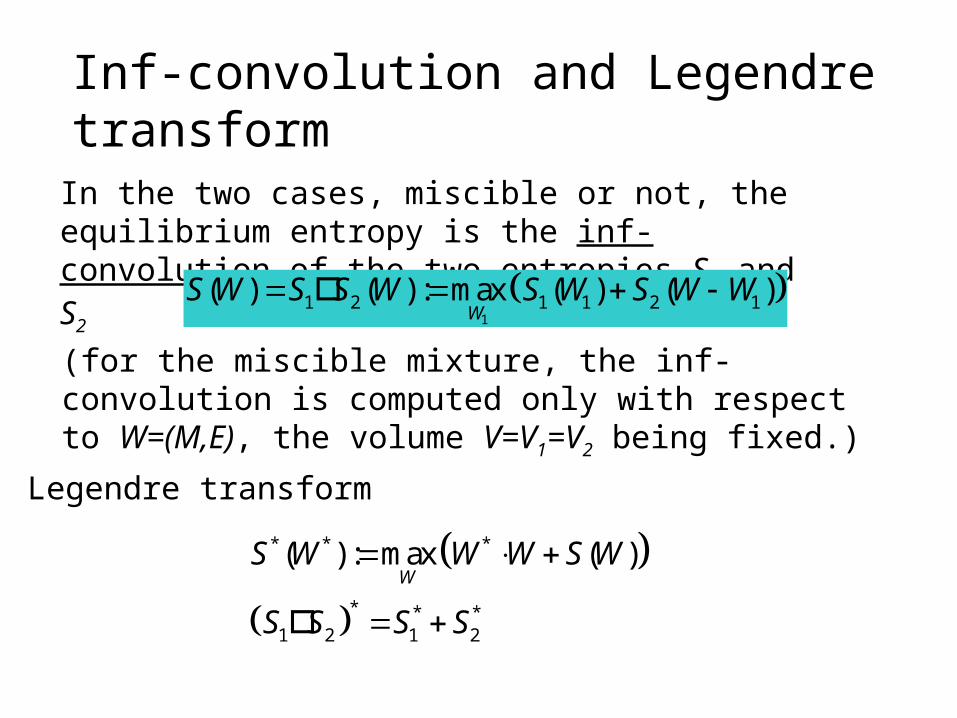
Inf-convolution and Legendre transform

* * *

* * *1 2 1 2

( ) : max ( )W

S W W W S W

S S S S

In the two cases, miscible or not, the equilibrium entropy is the inf-convolution of the two entropies S1 and S2

1

1 2 1 1 2 1( ) ( ) : max ( ) ( )W

S W S S W S W S W W

(for the miscible mixture, the inf-convolution is computed only with respect to W=(M,E), the volume V=V1=V2 being fixed.)

Legendre transform

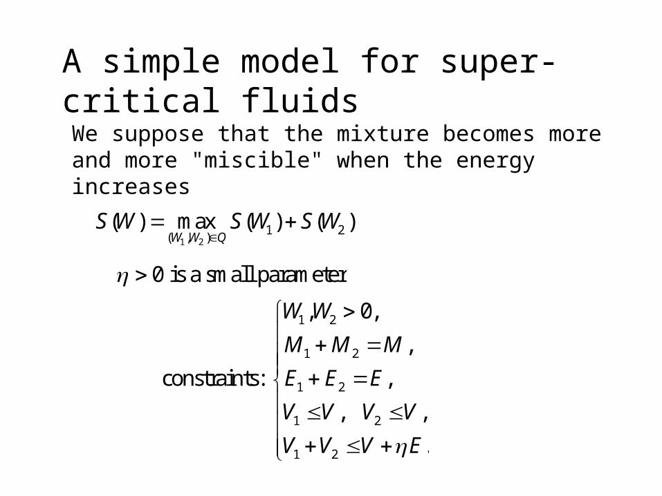
A simple model for super-critical fluids

We suppose that the mixture becomes more and more "miscible" when the energy increases

1 21 2

( , )( ) max ( ) ( )

W W QS W S W S W

1 2

1 2

1 2

1 2

1 2

, 0,

,

constraints: ,

, ,

.

W W

M M M

E E E

V V V V

V V V E

0 is a small parameter

Optimisation problem in intensive variables

1 21 2

1( , , ) ( , ) (1 ) ( , )

1 1

z zs Y s s

1 2( , , , )TY z

1

2

1 2

0 1,

0 1,

0 1,

0 1,

0 1 .

z

constraints

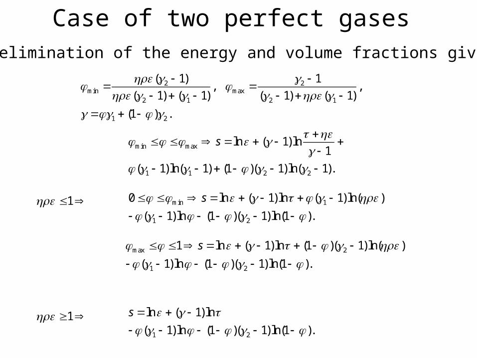
Case of two perfect gasesThe elimination of the energy and volume fractions gives

2 2min max

2 1 2 1

1 2

( 1) 1, ,

( 1) ( 1) ( 1) ( 1)

(1 ) .

min max

1 1 2 2

ln ( 1)ln1

( 1)ln( 1) (1 )( 1) ln( 1).

s

min 1

1 2

0 ln ( 1)ln ( 1)ln( )

( 1)ln (1 )( 1)ln(1 ).

s

max 2

1 2

1 ln ( 1)ln (1 )( 1) ln( )

( 1)ln (1 )( 1)ln(1 ).

s

1 2

ln ( 1) ln

( 1)ln (1 )( 1)ln(1 ).

s

1

1

Isothermal lines in the (,p) plane

p

critical point

saturation"liquid"

"gas" critical isotherm

super-critical fluid

In the saturation zone: modified isobaric pressure law

In the "liquid" zone the two phases are present

In the "gas" zone the two phases are present

In the super-critical zone: Dalton's law

*1 2

*

*

,

.1

p p p

pp

p

2

1

.1

pp

p

1

2

.1

pp

p

1 2.p p p

Conclusion

•the relaxation scheme expresses on the discrete level the physical entropy production.•it seems to converge towards the Liu solution•it is possible to implement the scheme in realistic configurations•the qualitative features of super-critical fluids can be recovered with the entropy optimisation procedure

Prospects

obtaining a precise critical behavior is still a challenging difficulty