Embed Size (px)
Citation preview

Numerical Simulation of Complex and Multiphase Flows
Numerical Simulation of Complex and Multiphase Flows.
IGESA. Porquerolles. 18th - 22nd April 2005
Non Homogenous Riemann Solver to simulate two-phaseflows.
K. Mohamed(1), L. Quivy(1),(2), F. Benkhaldoun(1),(2)
(1) LAGA, Université Paris XIII, FRANCE(2) CMLA, ENS de Cachan, FRANCE
Porquerolles 2005 1

Numerical Simulation of Complex and Multiphase Flows
1 Introduction :
– Presentation of VF scheme for non hongeneous systems, using flux
values instead of eigenvectors.
– Scheme analysis.
– Numerical results in 1D and 2D.
Porquerolles 2005 2
Numerical Simulation of Complex and Multiphase Flows
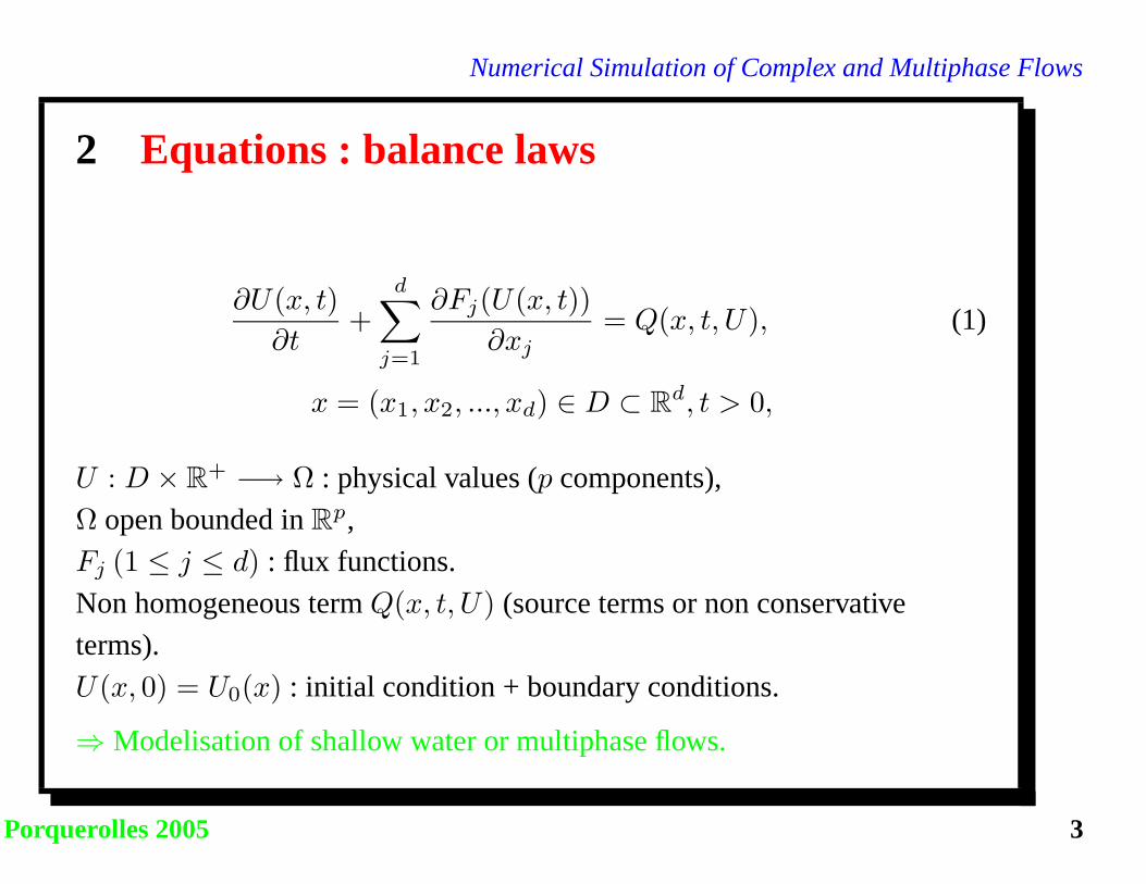
2 Equations : balance laws
∂U(x, t)
∂t+
d∑
j=1
∂Fj(U(x, t))
∂xj= Q(x, t, U), (1)
x = (x1, x2, ..., xd) ∈ D ⊂ Rd, t > 0,
U : D × R+ −→ Ω : physical values (p components),
Ω open bounded in Rp,
Fj (1 ≤ j ≤ d) : flux functions.
Non homogeneous term Q(x, t, U) (source terms or non conservative
terms).
U(x, 0) = U0(x) : initial condition + boundary conditions.
⇒Modelisation of shallow water or multiphase flows.
Porquerolles 2005 3

Numerical Simulation of Complex and Multiphase Flows
1D uniform case :∂U
∂t+∂F (U)
∂x= Q(x,U), 0 < t < T,
U(x, 0) = U0(x), ∀x ∈ Ω ⊂ R.
SRNHR schemeUnj+ 1
2=
1
2(Unj + Unj+1)−
αnj+ 1
2
2Snj+ 1
2
[F (Unj+1)− F (Unj )
]+αnj+ 1
2
2
∆x
Snj+ 1
2
Qnj+ 12
Un+1j = Unj − rn
[F (Unj+ 1
2)− F (Unj− 1
2)]
+ τnQnj ,
where Snj+ 1
2
= maxp=1,...,m
(∣∣λnp,i∣∣ ,∣∣λnp,i+1
∣∣) : local Rusanov velocity,
αnj+ 1
2
real and positive parameter, rn = τn
∆x .
Remark : αnj+ 1
2
is a parameter which aims to control numerical diffusion of
scheme.For example, for linear scalar equation on uniform mesh, αn
j+ 12
= 1
corresponds to Lax-Wendroff scheme.
Porquerolles 2005 4

Numerical Simulation of Complex and Multiphase Flows
3 Scheme analysis :Hypothesis : (scalar case)H1) f ′ and f” have a constant sign and does not vanish.H2) u0 has a constant sign and does not vanish. Suppose that0 < um ≤ u0(x) ≤ uM .
Proposition 3.1 Suppose that αnj+ 1
2
= (αnj+ 1
2
)1 =Snj+ 1
2
snj+ 1
2
, ∀j, ∀n, with
Snj+ 12
= max(|f ′(unj )|, |f ′(unj+1)|
)and
snj+ 12
= min(|f ′(unj )|, |f ′(unj+1
)|).
Denoting by αn = sup(j∈Z)
Snj+ 1
2
snj+ 1
2
, αmax =fpMfpm
,
fpm = min(|f ′(um)|, |f ′(uM )|), fpM = max(|f ′(um)|, |f ′(uM )|) and
M = sup | f ′(w) |, w ∈ w inR/ |w| ≤ αmax ‖ u0 ‖∞.Then, under condition αnMrn ≤ 1, SRNHR scheme is TV D, satisfy
maximum principle and then is L∞ stable.
Porquerolles 2005 5

Numerical Simulation of Complex and Multiphase Flows
Proposition 3.2 Suppose now that αnj+ 1
2
= (αnj+ 1
2
)2 = rnSnj+ 1
2
. Then
scheme SRNHR writes
unj+ 1
2
= 12 (unj + unj+1)− rn
2
[f(unj+1)− f(unj )
]
un+1j = unj − rn
[f(un
j+ 12
)− f(unj− 1
2
)].
which is secund order Richtmeyer scheme.
Then, the use of limiter theory :
αnj+ 12
= Φj(αnj+ 1
2)1 + (1− Φj) (αnj+ 1
2)2 (2)
where Φj is a limiter function (Superbee, Van-Leer,...).
Porquerolles 2005 6

Numerical Simulation of Complex and Multiphase Flows
4 Stationnary states preserving :
For Saint-Venant equations :
∂h
∂t(x, t) +
∂hu
∂x(x, t) = 0
∂hu
∂t(x, t) +
∂(hu2 + gh2
2 )
∂x(x, t) = −gh(x, t)
dz
dx(x)
h0(x), u0(x), z(x) given
Proposition 4.1 Under condition that source term is discretized as
Qnj = − 1
8∆xg(unj−1 + 2unj + unj+1)(zj+1 − zj−1)
SRNHR scheme satisfy exact C-property.
Riemann invariants for Saint-Venant equations are Wk = u+ (−1)k2c.
Porquerolles 2005 7

Numerical Simulation of Complex and Multiphase Flows
At step n, for each cell, local Rusanov velo-
city : Snj+ 1
2= max
p
(max
(|λnp,j |, |λnp,j+1|
))
If (Wkj+1 = Wkj ) then
θWk = 0
elseVelocity at interface :
cj+ 12
=√ghj+hj+1
2,
Vj+ 12
=(uj+uj+1)
2,
λkj+ 1
2
= Vj+ 12
+ (−1)k cj+ 12
If (λkj+ 1
2
> 0) then
θWk =Wkj
−Wkj−1
Wkj+1−Wkj
elseθWk =
Wkj+2−Wkj+1
Wkj+1−Wkj
end Ifend If
sj+ 12
= min(|λ1j+ 1
2
|, |λ2j+ 1
2
|)If (sj+ 1
2< ε ) then
sj+ 12
= ε
end IfIf (θW1 < 0 or θW2 < 0) then
φ = 0
else
φ = limiter functionend Ifαnj+ 1
2=
Snj+ 1
2sj+ 1
2
(1− φ) + φrnSnj+ 1
2.
Porquerolles 2005 8

Numerical Simulation of Complex and Multiphase Flows
5 1D homogeneous Saint-Venant equations :
Consider a dam break with solution containing a shock wave and a
rarefaction wave.
∂h
∂t(x, t) +
∂(hu)
∂x(x, t) = 0
∂(hu)
∂t(x, t) +
∂(hu2 + gh2
2
)
∂x(x, t) = 0
(3)
with initial conditions : h0(x) =
6 if x ≤ 6
2 if x > 6., and u0(x) = 0, ∀x.
Mesh contains 100 points and results are given at t = 0.4.
Porquerolles 2005 9

Numerical Simulation of Complex and Multiphase Flows
0 2 4 6 8 10 122
2.5
3
3.5
4
4.5
5
5.5
6Hauteur de l’eau, SRNHR, t=0.4, np=100
solution exacteSRNHR−alpha limiteROE
Homogeneous Shallow Water,
water level, SRNHR and Roe
schemes.
0 2 4 6 8 10 120
0.5
1
1.5
2
2.5
3
3.5solution exacteSRNHR−alpha limiteROE
Homogeneous Shallow Water,
water velocity, SRNHR and Roe
schemes.
Porquerolles 2005 10
Numerical Simulation of Complex and Multiphase Flows
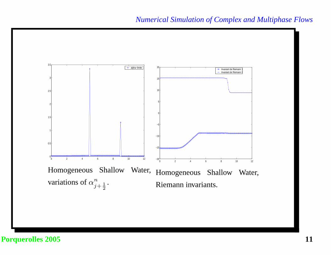
0 2 4 6 8 10 120
0.5
1
1.5
2
2.5
3
3.5alpha−limite
Homogeneous Shallow Water,
variations of αnj+ 1
2.
0 2 4 6 8 10 12−20
−15
−10
−5
0
5
10
15
20Invariant de Riemann 1Invariant de Riemann 2
Homogeneous Shallow Water,
Riemann invariants.
Porquerolles 2005 11
Numerical Simulation of Complex and Multiphase Flows
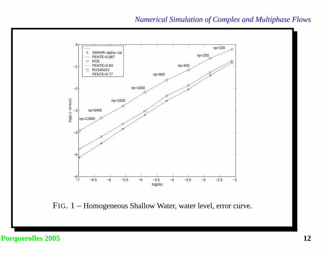
−7 −6.5 −6 −5.5 −5 −4.5 −4 −3.5 −3 −2.5 −2−6
−5
−4
−3
−2
−1
0
log(dx)
log
(L1
−e
rre
ur)
SRNHR−alpha−cstPENTE=0.887ROEPENTE=0.83RUSANOV PENTE=0.77
np=100
np=200
np=400
np=800
np=1600
np=3200
np=6400
np=12800
FIG. 1 – Homogeneous Shallow Water, water level, error curve.
Porquerolles 2005 12

Numerical Simulation of Complex and Multiphase Flows
6 1D homogeneous Euler equations :
Shock tube with initial conditions
ρ0(x, y) =
1 kg/m3 si x ≤ 0
0.01 kg/m3 si x > 0,
u0(x, y) = 0m/s, ∀x ∈ [−10; 10],
P0(x, y) =
105 Pa si x ≤ 0
103 Pa si x > 0,
Mesh : 800 points ; cfl = 0.95 ; t = 0.01.
Comparaison between SRNHR scheme and VFRoe scheme.
First characteristic field is a rarefaction wave which contains a sonic point.
Roe scheme needs to add entropic correction.
Porquerolles 2005 13

Numerical Simulation of Complex and Multiphase Flows
−10 −8 −6 −4 −2 0 2 4 6 8 100
0.1
0.2
0.3
0.4
0.5
0.6
0.7
0.8
0.9
1Densité du fluide, CFL=0.75, t=0.01, Maill=400
SRNHR ROE
Fluid density ; SRNHR and Roe
schemes.
−10 −8 −6 −4 −2 0 2 4 6 8 100
100
200
300
400
500
600
700Vitesse du fluide, CFL=0.75,T=0.01, MAILLAGE=400
SRNHR ROE
Fluid velocity ; SRNHR and Roe
schemes.
Porquerolles 2005 14

Numerical Simulation of Complex and Multiphase Flows
7 1D non homogeneous Saint-Venant
equations :Consider a dam break over a step. Source term describes bottom geometry.
∂h
∂t(x, t) +
∂(hu)
∂x(x, t) = 0
∂(hu)
∂t(x, t) +
∂(hu2 + gh2
2 )
∂x(x, t) = −gh(x, t)
dz
dx(x)
z(x) =
0 if x ≤ 6
1 if x > 6
h0(x) =
5 if x ≤ 6
1 if x > 6.
u0(x) = 0.
(4)
Porquerolles 2005 15
Numerical Simulation of Complex and Multiphase Flows
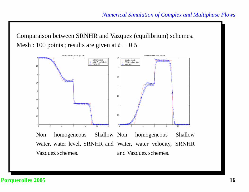
Comparaison between SRNHR and Vazquez (equilibrium) schemes.
Mesh : 100 points ; results are given at t = 0.5.
0 2 4 6 8 10 121
1.5
2
2.5
3
3.5
4
4.5
5Hauteur de l’eau, t=0.5, np= 100
solution exacteSRNHR−alpha limiteVAZQUEZ
Non homogeneous Shallow
Water, water level, SRNHR and
Vazquez schemes.
0 2 4 6 8 10 120
0.5
1
1.5
2
2.5
3
3.5Vitesse de l’eau, t=0.5, np=100
solution exacteSRNHR−alpha limiteVAZQUEZ
Non homogeneous Shallow
Water, water velocity, SRNHR
and Vazquez schemes.
Porquerolles 2005 16

Numerical Simulation of Complex and Multiphase Flows
−5 −4.5 −4 −3.5 −3 −2.5 −2−3.5
−3
−2.5
−2
−1.5
−1
−0.5
0
log(dx)
log
(L1
−E
rre
ur)
SRNHR−alpha limitéPente=0.82SRNHR−alpha=1.1Pente=0.734VazquezPente=0.51
np=100
np=200
np=400
np=800
np=1600
FIG. 2 – Non homogeneous Shallow Water, error curve, (water level), SRNHR and
Vazquez schemes.
Porquerolles 2005 17

Numerical Simulation of Complex and Multiphase Flows
8 2D SRNHR schemeNon homogeneous Saint-Venant equations :
∀(x, y) ∈ Ω ⊂ R2, t ∈ R+,
∂h
∂t(x, y, t) +
∂(hu)
∂x(x, y, t) +
∂hv
∂y(x, y, t) = 0
∂(hu)
∂t(x, y, t) +
∂(hu2 + 12gh2)
∂x(x, y, t) +
∂hv
∂y(x, y, t) = −gh(x, y, t)
dz
dx(x, y)
∂(hv)
∂t(x, y, t) +
∂hv
∂x+∂(hv2 + 1
2gh2)
∂y(x, y, t) = −gh(x, y, t)
dz
dy(x, y)
(5)
with initial conditions
h(x, y, 0) = h0(x, y)
(hu)(x, y, 0) = (hu)0(x, y)
(hv)(x, y, 0) = (hv)0(x, y)
z(x, y) given.
Porquerolles 2005 18
Numerical Simulation of Complex and Multiphase Flows
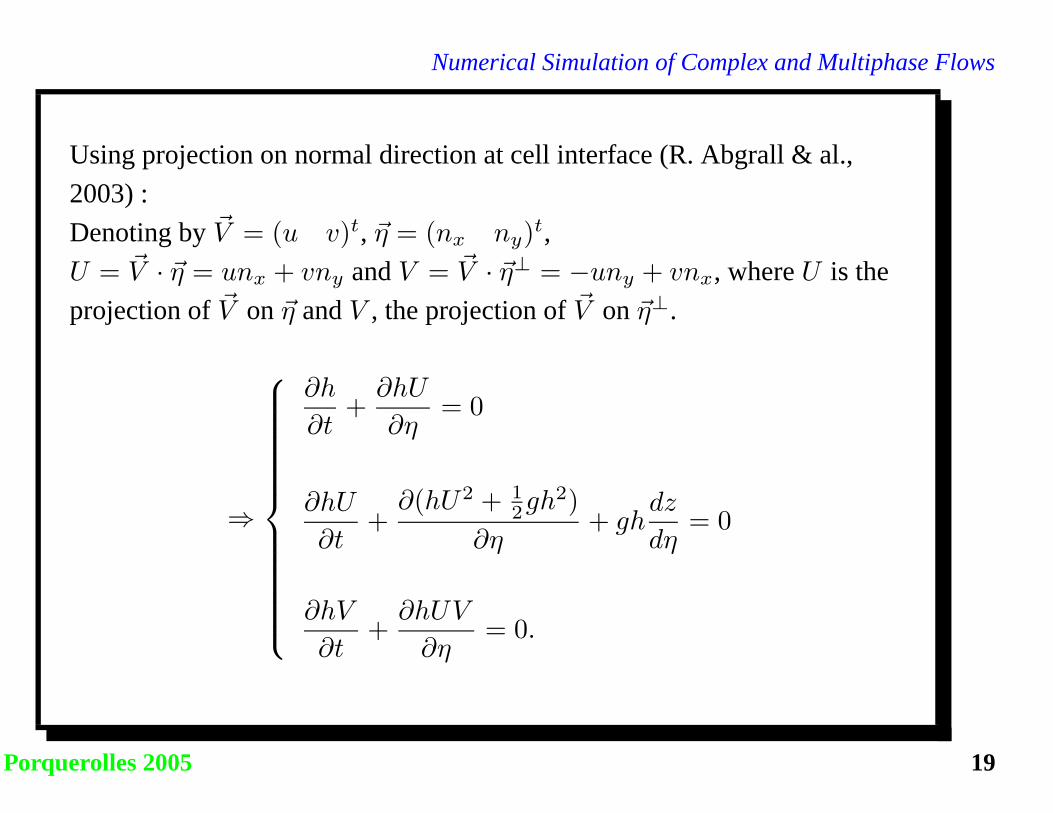
Using projection on normal direction at cell interface (R. Abgrall & al.,
2003) :
Denoting by ~V = (u v)t, ~η = (nx ny)t,
U = ~V · ~η = unx + vny and V = ~V · ~η⊥ = −uny + vnx, where U is the
projection of ~V on ~η and V , the projection of ~V on ~η⊥.
⇒
∂h
∂t+∂hU
∂η= 0
∂hU
∂t+∂(hU2 + 1
2gh2)
∂η+ gh
dz
dη= 0
∂hV
∂t+∂hUV
∂η= 0.
Porquerolles 2005 19

Numerical Simulation of Complex and Multiphase Flows
Numerical results :
Initial conditions : h0(x, y) =
6 if x ≤ 6, ∀y ∈ [0; 1]
2 if x > 6, ∀y ∈ [0; 1]
u0(x, y) = v0(x, y) = 0, ∀x ∈ [0; 12], ∀y ∈ [0; 1].
PSfrag replacements
12 m
zl = 0 m
zr = 1 mhr = 2 m
hl = 6 m
(u, v)l = (0, 0) m/s (u, v)r = (0, 0) m/s
Porquerolles 2005 20
Numerical Simulation of Complex and Multiphase Flows
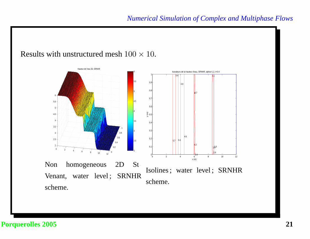
Results with unstructured mesh 100× 10.
0 2 4 6 8 10 120
0.2
0.4
0.6
0.8
1
2
2.5
3
3.5
4
4.5
5
5.5
6
Hauteur de l’eau 2D, SRNHR
2
2.5
3
3.5
4
4.5
5
5.5
6
Non homogeneous 2D St-
Venant, water level ; SRNHR
scheme.
0 2 4 6 8 10 120
0.1
0.2
0.3
0.4
0.5
0.6
0.7
0.8
0.9
1
2.3
2.6
2.9
3.1
3.4
3.74
4.3
4.6
4.9
5.1
5.4
5.7
x (m)
y (
m)
Isovaleurs de la hauteur d’eau, SRNHR, alpha=1.2, t=0.4
Isolines ; water level ; SRNHR
scheme.
Porquerolles 2005 21
Numerical Simulation of Complex and Multiphase Flows
0 2 4 6 8 10 120
0.2
0.4
0.6
0.8
1
−0.5
0
0.5
1
1.5
2
2.5
3Vitesse de l’eau 2D, SRNHR
0
0.5
1
1.5
2
2.5
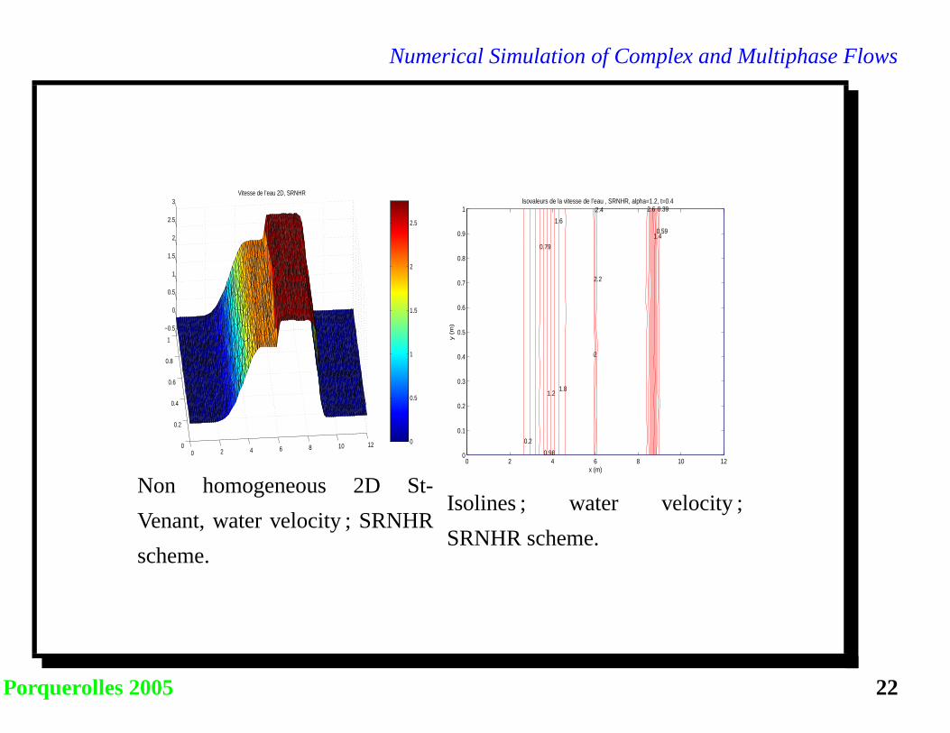
Non homogeneous 2D St-
Venant, water velocity ; SRNHR
scheme.
0 2 4 6 8 10 120
0.1
0.2
0.3
0.4
0.5
0.6
0.7
0.8
0.9
1
0.2
0.39
0.59
0.79
0.98
1.2
1.4
1.6
1.8
2
2.2
2.4 2.6
x (m)
y (
m)
Isovaleurs de la vitesse de l’eau , SRNHR, alpha=1.2, t=0.4
Isolines ; water velocity ;
SRNHR scheme.
Porquerolles 2005 22

Numerical Simulation of Complex and Multiphase Flows
0 2 4 6 8 10 120
0.2
0.4
0.6
0.8
1
−2
0
2
4
6
8
10
Débit 2D, SRNHR
0
1
2
3
4
5
6
7
8
9
Non homogeneous 2D St-
Venant, water flow ; SRNHR
scheme.
0 2 4 6 8 10 120
0.1
0.2
0.3
0.4
0.5
0.6
0.7
0.8
0.9
1 0.67
1.3
2
2.7
3.3
4
4.7
5.3
6
6.7
7.3 8
8.7
x (m)
y (
m)
Isovaleur du débit de l’eau, SRNHR, alpha=1.2, t=0.4
Isolines ; water flow ; SRNHR
scheme.
Porquerolles 2005 23

Numerical Simulation of Complex and Multiphase Flows
9 Two phase flow
1D case :
∂U
∂t+∂f(U)
∂x= Q1(x,U) +Q2(x,U)
U(x, 0) = U0(x)
(6)
with
U = (µvρv µvρvuv µlρl µlρlul)t,
f(U) = (µvρvuv µvρvu2v µlρlul µlρlu
2l )t,
Q1(x,U) = (0 − µv∂P
∂x0 − µl
∂P
∂x)t,
Q2(x,U) = (0 µvρvg 0 µlρlg)t.
Non hyperbolic and non conservative problem.
Porquerolles 2005 24

Numerical Simulation of Complex and Multiphase Flows
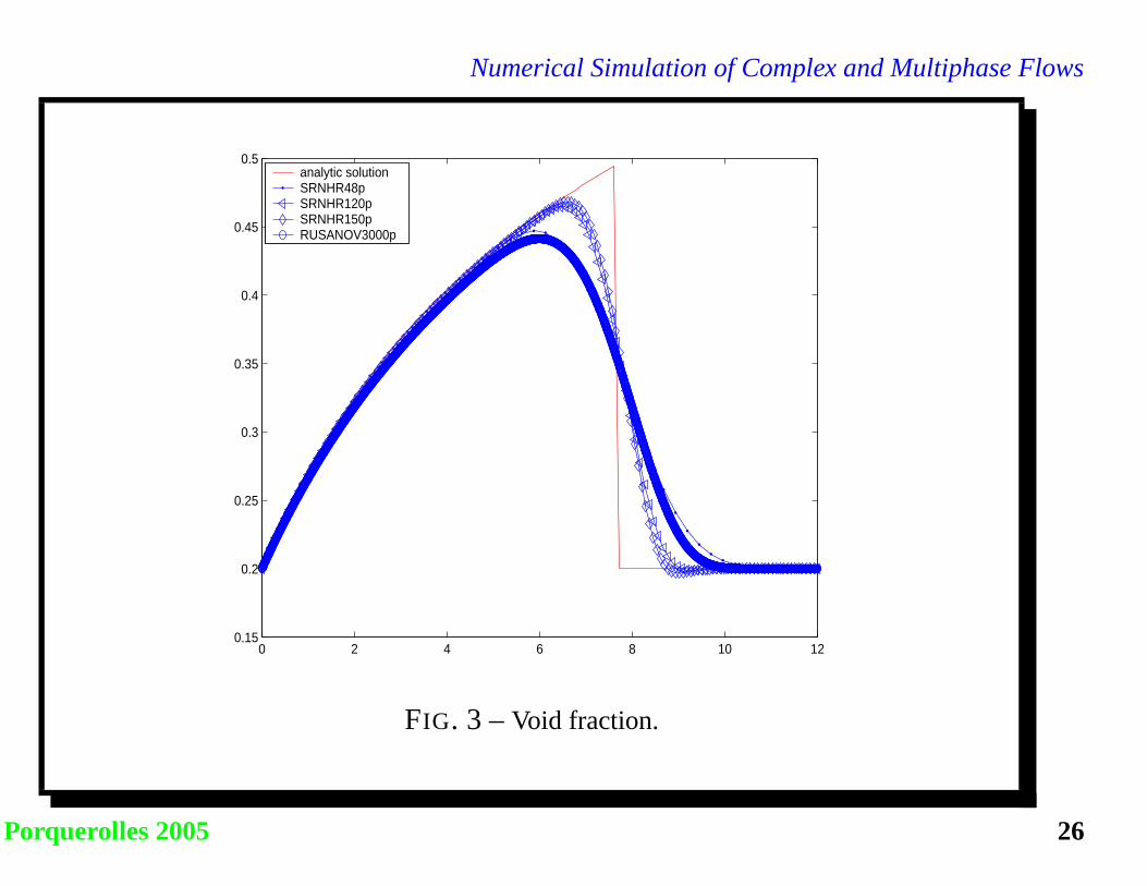
1D Ransom ProblemInitial condition :
∀x ∈ [x0, xl], µv(t = 0) = 0.2,
ul(t = 0) = 10,
uv(t = 0) = 0,
p(t = 0) = 105,
ρv(t = 0) = 1,
ρl(t = 0) = 988, 0638.
Boundary conditions :
– inlet (x0 = 0) :
µv(0, t) = 0.2,
ul(0, t) = 10, uv(0, t) = 0.
– outlet (xl = 12) :
p (12, t) = 105.
g
PSfrag replacements
inlet
outlet
g
12 m
ul = 10 m/svv = 0 m/s
µv = 0.2 m/s
P = 105Pa
gaz
liquid
Porquerolles 2005 25
Numerical Simulation of Complex and Multiphase Flows
0 2 4 6 8 10 120.15
0.2
0.25
0.3
0.35
0.4
0.45
0.5analytic solutionSRNHR48pSRNHR120pSRNHR150pRUSANOV3000p
FIG. 3 – Void fraction.
Porquerolles 2005 26

Numerical Simulation of Complex and Multiphase Flows
10 Discretization of source termSRNHR scheme :
Unj+ 12
= (νUnj + (1−ν)Unj+1)−αnj+ 1
2
2snj+ 1
2
[f(Unj+1)−f(Unj )
]−αnj+ 1
2
2
∆x
snj+ 1
2
Qnj+ 12
Un+1j = Unj − r
[f(Unj+ 1
2
)− f
(Unj− 1
2
))]
+ ∆tnQnj ,
Qnj =1
2∆x
(µnj)
(Pj+1 − Pj−1) (second step).
Qnj+ 12
=µnj+ 1
2
2
(Pj+1 − Pj)h
(first step).
µnj+ 1
2
: intermediate value between µnj and µnj+1.
To preserve stationnary states, 2 choices :
µnj+ 1
2
= 12 (µnj + µnj+1) : results given before.
µnj+ 1
2
= µnj+ 1
2
obtained with Unj+ 1
2
computed at same step→ better in this
case.
Porquerolles 2005 27

Numerical Simulation of Complex and Multiphase Flows
0 2 4 6 8 10 120.1
0.15
0.2
0.25
0.3
0.35
0.4
0.45
0.5Taux de vide,1D,t=0.6
solution exacteSRNHR−48pSRNHR−100pSRNHR−200pSRNHR−400p
Void fraction ; µnj+ 1
2= µn
j+ 12
.
−4 −3.5 −3 −2.5 −2 −1.5 −1 −0.5−2.6
−2.4
−2.2
−2
−1.8
−1.6
−1.4
−1.2
−1
−0.8
log(dx)lo
g(L
1−
Err
eu
r)
Courbe d’erreur, Taux de vide,SRNHR, cfl=0.5, t=0.6
SRNHR− choix 1PENTE=0.533
np=24
np=48
np=96
np=200
np=400
Error curve ; Void fraction ;
µnj+ 1
2= µn
j+ 12
.
Porquerolles 2005 28

Numerical Simulation of Complex and Multiphase Flows
11 Model with interfacial pressure
Source term writes now :
Q1(x,W ) = (0 −µv∂P
∂x−(P−Pi)∂µv∂x 0 −µl
∂P
∂x−(P−Pi)
∂µl∂x
)t,
Q2(x,W ) = (0 µvρvg 0 µlρlg)t,
with P − Pi = ρv(uv − ul)2 : interfacial pressure.
→ Hyperbolic problem
Porquerolles 2005 29

Numerical Simulation of Complex and Multiphase Flows
0 2 4 6 8 10 120.2
0.25
0.3
0.35
0.4
0.45
0.5Taux de vide, 1D,cfl=0.5, t=0.6
solution exacteSRNHR−200pSRNHR−500pSRNHR−1000pSRNHR−2000p
Void Fraction (with interfacial
pressure) ; µnj+ 1
2= µn
j+ 12
.
−5.5 −5 −4.5 −4 −3.5 −3 −2.5 −2 −1.5 −1 −0.5−2.8
−2.6
−2.4
−2.2
−2
−1.8
−1.6
−1.4
−1.2
−1
−0.8
log(dx)
log
(L1
−E
rre
ur)
Courbe d’erreur,Taux de vide avec la pression interfaciale, cfl=0.5, t=0.6
SRNHR −Choix 1PENTE=0.4 np=24
np=48
np=96
np=200
np=400
np=800
np=1600 np=2000
Error curve ; Void Fraction
(with interfacial pressure) ;
µnj+ 1
2= µn
j+ 12
.
Porquerolles 2005 30
Numerical Simulation of Complex and Multiphase Flows
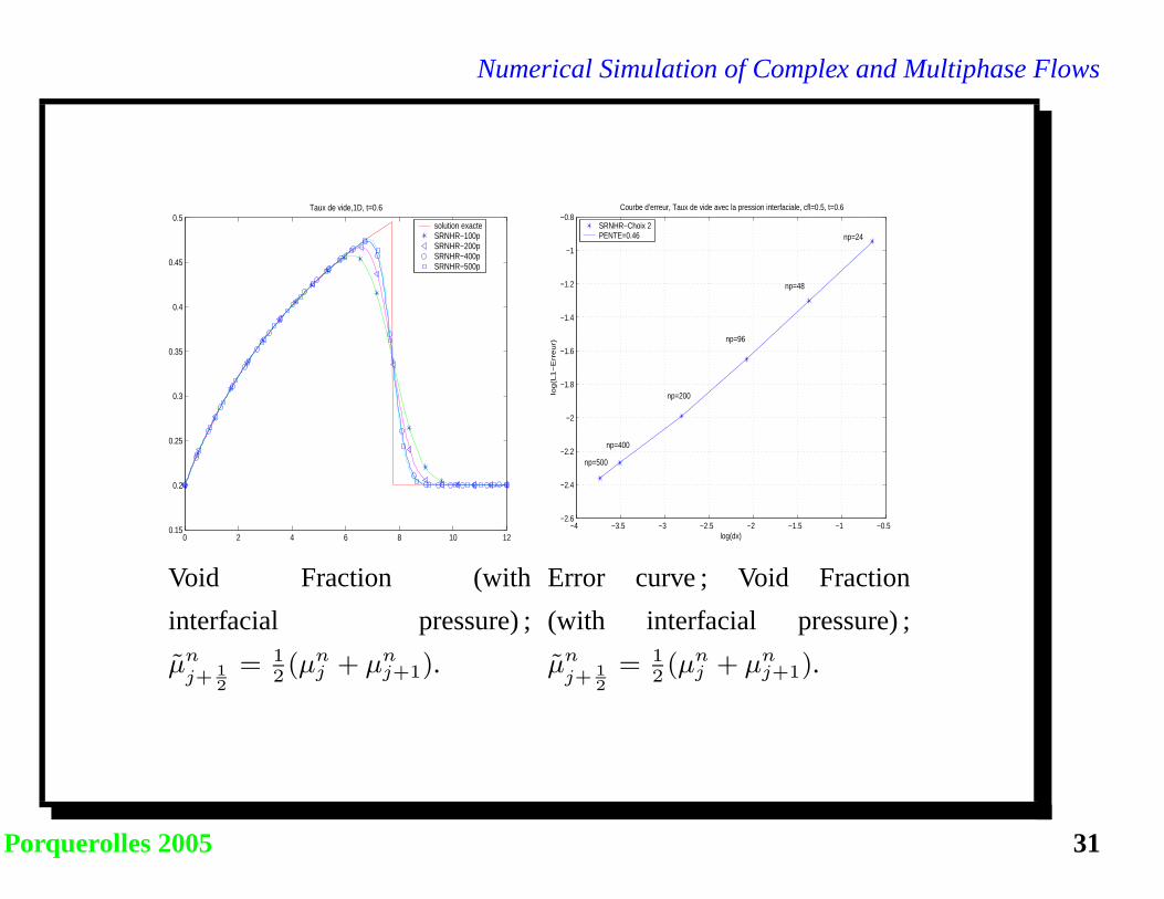
0 2 4 6 8 10 120.15
0.2
0.25
0.3
0.35
0.4
0.45
0.5Taux de vide,1D, t=0.6
solution exacteSRNHR−100pSRNHR−200pSRNHR−400pSRNHR−500p
Void Fraction (with
interfacial pressure) ;
µnj+ 1
2= 1
2(µnj + µnj+1).
−4 −3.5 −3 −2.5 −2 −1.5 −1 −0.5−2.6
−2.4
−2.2
−2
−1.8
−1.6
−1.4
−1.2
−1
−0.8
log(dx)
log
(L1
−E
rre
ur)
Courbe d’erreur, Taux de vide avec la pression interfaciale, cfl=0.5, t=0.6
SRNHR−Choix 2PENTE=0.46 np=24
np=48
np=96
np=200
np=400
np=500
Error curve ; Void Fraction
(with interfacial pressure) ;
µnj+ 1
2= 1
2(µnj + µnj+1).
Porquerolles 2005 31
Numerical Simulation of Complex and Multiphase Flows
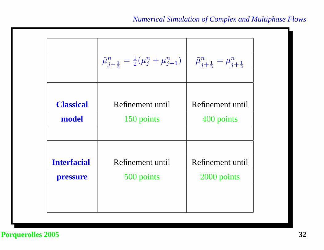
µnj+ 1
2
= 12 (µnj + µnj+1) µn
j+ 12
= µnj+ 1
2
Classical Refinement until Refinement until
model 150 points 400 points
Interfacial Refinement until Refinement until
pressure 500 points 2000 points
Porquerolles 2005 32
Numerical Simulation of Complex and Multiphase Flows
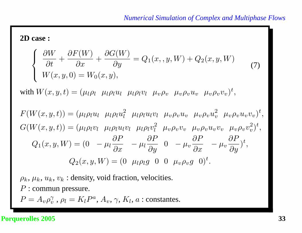
2D case :
∂W
∂t+∂F (W )
∂x+∂G(W )
∂y= Q1(x, , y,W ) +Q2(x, y,W )
W (x, y, 0) = W0(x, y),(7)
with W (x, y, t) = (µlρl µlρlul µlρlvl µvρv µvρvuv µvρvvv)t,
F (W (x, y, t)) = (µlρlul µlρlu2l µlρlulvl µvρvuv µvρvu
2v µvρvuvvv)
t,
G(W (x, y, t)) = (µlρlvl µlρlulvl µlρlv2l µvρvvv µvρvuvvv µvρvv
2v)t,
Q1(x, y,W ) = (0 − µl∂P
∂x− µl
∂P
∂y0 − µv
∂P
∂x− µv
∂P
∂y)t,
Q2(x, y,W ) = (0 µlρlg 0 0 µvρvg 0)t.
ρk, µk, uk, vk : density, void fraction, velocities.P : commun pressure.P = Avρ
γv , ρl = KlP
a, Av, γ, Kl, a : constantes.
Porquerolles 2005 33

Numerical Simulation of Complex and Multiphase Flows
µv = 0.6. UK Drag mesh 48× 10.
0 2 4 6 8 10 120
0.2
0.4
0.6
0.8
1
0.56
0.58
0.6
0.62
0.64
0.66
0.68
0.7
0.72
0.74
Taux de vide, SRNHR
0.6
0.62
0.64
0.66
0.68
0.7
0.72
Void fraction ; SRNHR scheme
(α = 2).
0 2 4 6 8 10 120
0.5
1
1.5
2
2.5
3
3.5
4Isovaleur de taux de vide
Void fraction ; Isolines ; SRNHR
scheme (α = 2).
Porquerolles 2005 34

Numerical Simulation of Complex and Multiphase Flows
0 2 4 6 8 10 12
0
0.2
0.4
0.6
0.8
1
10
11
12
13
14
15
16
Vitesse du liquide, SRNHR
10.5
11
11.5
12
12.5
13
13.5
14
14.5
15
15.5
Liquid velocity ; SRNHR scheme
(α = 2).
0 2 4 6 8 10 120
0.5
1
1.5
2
2.5
3
3.5
4Isovaleur de la vitesse du liquide
Liquid velocity ; Isolines ;
SRNHR scheme (α = 2).
Porquerolles 2005 35
Numerical Simulation of Complex and Multiphase Flows
Conclusion :
– Robust and efficient scheme for non homogeneous systems.
– Do not need calculus of jacobien fields decomposition.
– Accurate results obtained with few mesh points.
Porquerolles 2005 36


