Embed Size (px)
Citation preview

Numerical Simulation in Statistical Physics
Lecture in Master 2 “Physics of complex systems” and “Modeling,
Statistics and Algorithms for out-of-equilibrium systems.
Pascal ViotLaboratoire de Physique Theorique de la Matiere Condensee, Boıte 121,
4, Place Jussieu, 75252 Paris Cedex 05Email : [email protected]
October 26, 2015
These lecture notes provide an introduction to the methods of numerical simulation in classicalstatistical physics.
Based on simple models, we start in a first part on the basics of the Monte Carlo method andof the Molecular Dynamics. A second part is devoted to the introduction of the basic microscopicquantities available in simulation methods, and to the description of the methods allowing for studyingthe phase transitions. In a third part, we consider the study of out-of-equilibrium systems as well asthe characterization of the dynamics: in particular, aging phenomena are presented.
2

1Statistical mechanics and numerical simulation
1.1 Brief History of simulation
Numerical simulation started in the fifties when computers were used for the first time for peacefulpurposes. In particular, the computer MANIAC started in 1952 1 at Los Alamos. Simulation pro-vides a complementary approach to theoretical methods 2. Areas of physics where the perturbativeapproaches are efficient (dilute gases, vibrations in quasi-harmonic solids) do not require simulationmethods. Conversely, liquid state physics, where few exact results are known and where the theoreticaldevelopments are not always under control, has been developed largely through simulation. The firstMonte Carlo simulation of liquids was performed by Metropolis et al. in 1953 3.
The first Molecular Dynamics was realized on the hard disk model by Alder and Wainwright in1957[1]. The first Molecular Dynamics of a simple liquid (Argon) was performed by Rahman in 1964.In these last two decades, the increasing power of computers associated with their decreasing costs
allowed numerical simulations with personal computers. Even if supercomputers are necessary forextensive simulations, it becomes possible to perform simulations on low cost computers. In orderto measure the power of computers, the unit of performance is the GFlops (or billion of floatingpoint operations per second). Nowadays, a Personal computer PC (for instance, Intel Core i7) has aprocessor with four cores (floating point unit) and offers a power of 24 Gflops. Whereas the frequencyof processors seems to have plateaued last few years, power of computers continues to increase becausethe number of cores within a processor grows. Nowadays, processors with 6 or 8 cores are available.In general, the power of a computer is not a linear function of cores for many programs. For scientificcodes, it is possible to exploit this possibility by developing scientific programs incorporating librarieswhich perform parallel computing (OpenMP, MPI). The gnu compilers are free softwares allowingfor parallel computing. For massive parallelism, MPI (message passing interface) is a library whichspreads the computing load over many cores.
It is worth noting that the rapid evolution of the power of the computers. In 2009, only onecomputer exceeded the PFlops, while they are 37 in 2014. the world in 2014 with a power rate of 33PFlops.
1. The computer MANIAC is the acronym of ”mathematical and numerical integrator and computer”. MANIAC Istarted March 15, 1952.
2. Sometimes, theories are in their infancy and numerical simulation is the sole manner for studying models3. Metropolis, Nicholas Constantine (1915-1999) both mathematician and physicist of education was hired by J.
Robert Oppenheimer at the Los Alamos National Laboratory in April 1943. He was one of scientists of the ManhattanProject and collaborated with Enrico Fermi and Edward Teller on the first nuclear reactors. After the war, Metropoliswent back to Chicago as an assistant professor, and returned to Los Alamos in 1948 by creating the Theoretical Division.He built the MANIAC computer in 1952, then 5 years later MANIAC II. He returned from 1957 to 1965 to Chicago andfounded the Computer Research division, and finally, returned to Los Alamos.
3

Statistical mechanics and numerical simulation
1.2 Ensemble averages in a nutshell
Knowledge of the partition function of a system allows one to obtain all thermodynamic quanti-ties. First, we briefly review the main ensembles used in Statistical Mechanics. We assume that thethermodynamic limit leads to the same quantities, a property for systems where interaction betweenparticles are not long ranged or systems without quenched disorder.
For finite size systems (which correspond to those studied in computer simulation), there aredifferences that we will analyze in the following.
1.2.1 Microcanonical ensemble
The system is characterized by the set of macroscopic variables: volume V , total energy E and thenumber of particles N . This ensemble is not appropriate for experimental studies, where one generallyhas
— a fixed number of particles, but a fixed pressure P and temperature T . This corresponds to aset of variables (N,P, T ) and is the isothermal-isobaric ensemble,
— a fixed chemical potential µ, volume V and temperature T , ensemble (µ, V, T ) or grand canon-ical ensemble,
— a fixed number of particles, a given volume V and temperature T , ensemble (N,V, T ) or canon-ical ensemble.
The partition function Z(E, V,N) is
Z(E, V,N) =∑α
δ(E − Eα) (1.1)
where δ is a Kronecker symbol (equal to 1 when (E−Eα) = 0 and 0 when (E−Eα) 6= 0. Note that allmicrostates have the same weight for computing the partition function. The associated thermodynamicpotential is the entropy given by
S(E, V,N) = kB ln(Z(E, V,N)) (1.2)
where kB is the Boltzmann constant.
The variables conjugated to the global quantities defining the ensemble fluctuate in time. Forthe micro-canonical ensemble, this corresponds to the pressure P conjugate to the volume V , to thetemperature T conjugate to the energy E and to the chemical potential µ conjugate to the totalnumber of particles N .
1.2.2 Canonical ensemble
The system is characterized by the following set of variables: the volume V ; the temperature Tand the total number of particles N . If we denote the Hamiltonian of the system H, the partitionfunction reads
Q(V, β,N) =∑α
exp(−βH(α)) (1.3)
where β = 1/kBT (kB is the Boltzmann constant). The sum runs over all configurations of thesystem. If this number is continuous, the sum is replaced with an integral. α denotes the index ofthese configurations. The free energy F (V, β,N) of the system is equal to
βF (V, β,N) = − ln(Q(V, β,N)). (1.4)
4

1.2 Ensemble averages in a nutshell
One defines the probability of having a configuration α as
p(V, β,N ;α) =exp(−βH(α))
Q(V, β,N). (1.5)
where H(α) denotes the energy of the configuration α. One easily checks that the basic properties ofa probability are satisfied, i.e.
∑α p(V, β,N ;α) = 1 and p(V, β,N ;α) > 0.
The derivatives of the free energy are related to the moments of this probability distribution, whichgives a microscopic interpretation of the macroscopic thermodynamic quantities. The mean energyand the specific heat are then given by
— Mean energy
U(V, β,N) = 〈H(α)〉 =∂(βF (V, β,N))
∂β
U =∑α
H(α)p(V, β,N ;α) (1.6)
— Specific heat
Cv(V, β,N) = −kBβ2∂U(V, β,N)
∂β= kBβ
2(〈H(α)2〉 − 〈H(α)〉2
)
Cv = kBβ2
∑α
H2(α)p(V, β,N ;α)−
(∑α
H(α)p(V, β,N ;α)
)2 (1.7)
1.2.3 Grand canonical ensemble
The system is then characterized by the following set of variables: the volume V , the temperatureT and the chemical potential µ. Let us denote the Hamiltonian HN the Hamiltonian of N particles,the grand partition function Ξ(V, β, µ) reads:
Ξ(V, β, µ) =∞∑N=0
∑αN
exp(−β(HN (αN )− µN)) (1.8)
where β = 1/kBT (kB is the Boltzmann constant) and the sum run over all configurations of Nparticles and over all configurations for systems having a number of particles going from 0 to infty.The grand potential is equal to
βΩ(V, β, µ) = − ln(Ξ(V, β, µ)) (1.9)
In a similar way, one defines the probability (distribution) P (V, β, µ;αN ) of having a configurationαN (with N particles) by the relation
p(V, β, µ;αN ) =exp(−β(HN (αN )− µN))
Ξ(V, β, µ)(1.10)
The derivatives of the grand potential can be expressed as moments of the probability distribution
5

Statistical mechanics and numerical simulation
— Mean number
〈N(V, β, µ)〉 = −∂(βΩ(V, β, µ))
∂(βµ)=∑N
∑αN
p(V, β, µ;αN ) (1.11)
— Susceptibility
χ(V, β, µ) =β
〈N(V, β, µ)〉ρ∂〈N(V, β, µ)〉
∂βµ=
β
〈N(V, β, µ)〉ρ(〈N2(V, β, µ)〉 − 〈N(V, β, µ)〉2
)(1.12)
χ(V, β, µ) =β
〈N(V, β, µ)〉ρ
∑N
∑αN
N2p(V, β, µ;αN )−
(∑N
∑αN
Np(V, β, µ;αN )
)2
(1.13)
1.2.4 Isothermal-isobaric ensemble
The system is characterized by the following set of variables: the pressure P , the temperature T andthe total number of particles N . Because this ensemble is generally devoted to molecular systems andnot used for lattice models, one only considers continuous systems. The partition function reads:
Q(P, β,N) =βP
Λ3NN !
∫ ∞0
dV exp(−βPV )
∫ V
0drN exp(−βU(rN )) (1.14)
where β = 1/kBT (kB is the Boltzmann constant). The Gibbs potential is equal to
βG(P, β,N) = − ln(Q(P, β,N)). (1.15)
One defines the probability p(P, β, µ;αV ) of having a configuration αV ≡ rN (particle positionsrN ), with a temperature T and a pressure P ).
p(P, β, µ;αV ) =exp(−βV ) exp(−β(U(rN )))
Q(P, β,N). (1.16)
The derivatives of the Gibbs potential are expressed as moments of this probability distribution.Therefore,
— Mean volume
〈V (P, β,N)〉 =∂(βG(P, β,N))
∂βP(1.17)
〈V (P, β,N)〉 =
∫ ∞0
dV V
∫ V
0drNΠ(P, β, µ;αV ). (1.18)
This ensemble is appropriate for simulations which aim to determine the equation of state of a system.Let us recall that a statistical ensemble can not be defined from a set of intensives variables only.However, we will see later that a technique so called Gibbs ensemble method is close in spirit of suchan ensemble (with the difference we always consider in simulation finite systems).
6

1.3 Model systems
1.3 Model systems
We restrict the lecture notes to classical statistical mechanics, which means that the quantumsystems are not considered here. In order to provide many illustrations of successive methods, weintroduce several basic models that we consider several times in the following
1.3.1 Simple liquids and Lennard-Jones potential
A simple liquid is a system of N point particles labeled from 1 to N , of identical mass m, interactingwith an external potential U1(ri) and among themselves by a pairwise potential U2(ri, rj) (i.e. apotential where the particles only interact by pairs). The Hamiltonian of this system reads:
H =N∑i=1
[p2i
2m+ U1(ri)
]+
1
2
∑i 6=j
U2(ri, rj), (1.19)
where pi is the momentum of the particle i. For instance, in the grand canonical ensemble, thepartition function Ξ(µ, β, V ) is given by
Ξ(µ, β, V ) =∞∑N=0
1
N !
∫ N∏i=1
(ddpi)(ddri)
hdNexp(−β(H− µN)) (1.20)
where h is the Planck constant and d the space dimension. The integral over the momentum can beobtained analytically, because there is factorization of the multidimensional integral on the variablespi. The one-dimensional integral of each component of the momentum is a Gaussian integral. Usingthe thermal de Broglie length
ΛT =h√
2πmkBT, (1.21)
one has ∫ +∞
−∞
ddp
hdexp(−βp2/(2m)) =
1
ΛdT. (1.22)
The partition function can be reexpressed as
Ξ(µ, β, V ) =∞∑N=0
1
N !
(eβµ
ΛdT
)NZN (β,N, V ) (1.23)
where ZN (β,N, V ) is called the configuration integral.
ZN (β,N, V ) =
∫drN exp(−βU(rN )) (1.24)
One defines z = eβµ as the fugacity. The thermodynamic potential associated with the partitionfunction, Ω(µ, β, V ), is
Ω(µ, β, V ) = − 1
βln(Ξ(µ, β, V )) = −PV (1.25)
where P is the pressure. Note that, for classical systems, only the part of the partition functionwith the potential energy is non-trivial. Moreover, there is decoupling between the kinetic part andpotential part, contrary to the quantum statistical mechanics.
To determine the phase diagram composed of different regions (liquid phase, gas and solid phases),the interaction potential between particles must contain a repulsive short-range interaction and anattractive long-range interaction. The physical interpretation of these contributions is the following:at short distance, quantum mechanics prevent atom overlap which explains the repulsive part of the
7

Statistical mechanics and numerical simulation
potential. At long distance, even for neutral atoms, the London forces (whose origin is also quantummechanical) are attractive. A potential satisfying these two criteria, is the Lennard-Jones potential
u(r) = 4ε
[(σr
)12−(σr
)6]
(1.26)
where ε defines a microscopic energy scale and σ denotes the atom diameter (see Fig.1.1).
0.5 1.0 1.5 2.0 2.5 3.0 3.5 4.0r/σ
1
0
1
2
3
4
u(r
)/ε
Figure 1.1 – Reduced Lennard-Jones potentialu(r)/ε versus r/σ.
import numpy as np
import matplotlib.pylab as plt
def lj(x):
return 4*(x**(-12)-x**(-6))
x= np.arange(0.8,4.0,0.01)
plt.ylim(-1,4)
plt.plot(x,lj(x))
plt.show()
plt.xlabel(’$r/\sigma$’,fontsize=20)
plt.ylabel(’$u(r)/\epsilon$’,fontsize=20)
plt.plot([0.5,4],[0,0])
As usual, in simulation, all quantities are expressed in dimensionless units: temperature is thenT ∗ = kBT/ε where kB is the Boltzmann constant, the distance is r∗ = r/σ and the energy is u∗ = u/ε.The three-dimensional Lennard-Jones model has a critical point at T ∗c = 1.3 and ρ∗c = 0.3, and a triplepoint T ∗t = 0.6 and ρ∗t = 0.8
1.3.2 Ising model and lattice gas. Equivalence
The Ising model is a lattice model where sites are occupied by particles with very limited degreesof freedom. Indeed, the particle is characterized by a spin which is a two-state variable (−1,+1). Eachspin interacts with its nearest neighbors and with a external field H, if it exists. The Ising model,initially introduced for describing the behavior of para-ferromagnetic systems, can be used in manyphysical situations The Hamiltonian is given by
H = −J∑<i,j>
SiSj −HN∑i=1
Si (1.27)
where the summation < i, j > means that the interaction is restricted to distinct pairs of nearestneighbors and H denotes an external uniform field. If J > 0, interaction is ferromagnetic and if J < 0,interaction is antiferromagnetic.
In one dimension, this model can be solved analytically and one shows that the critical temperatureis the zero temperature.
In two dimensions, Onsager (1944) solved this model in the absence of an external field and showedthat there exists a para-ferromagnetic transition at a finite temperature. For the square lattice, thiscritical temperature is given by
Tc = J2
ln(1 +√
2)(1.28)
and a numerical value equal to Tc ' 2.269185314 . . . J .In three dimensions, the model can not be solved analytically, but numerical simulations have been
performed with different algorithms and the values of the critical temperature obtained for variouslattices and from different theoretical methods are very accurate (see Table 1.1).
8

1.3 Model systems
D Lattice Tc/J (exact) Tc,MF /J
1 0 22 square 2.269185314 42 triangular 3.6410 62 honeycomb 1.5187 33 cubic 4.515 63 bcc 6.32 83 diamond 2.7040 44 hypercube 6.68 8
Table 1.1 – Critical Temperatures of the Ising model for different lattices in 1 to 4 dimensions.
A useful, but crude, estimate of the critical temperature is given by the mean-field theory
Tc = cJ (1.29)
where c is the coordination number.Table 1.1 illustrates that the critical temperatures predicted by the mean-field theory are always
an upper bound of the exact values and that the quality of the approximation becomes better whenthe spatial dimension of the system is large and/or the coordination number is large.
The lattice gas model was introduced by Lee and Yang. The basic idea, greatly extended later,consists of assuming that the macroscopic properties of a system with a large number of particles donot crucially depend on the microscopic details of the interaction. By performing a coarse-graining ofthe microscopic system, one builds an effective model with a smaller number of degrees of freedom.This idea is often used in statistical physics, because it is often necessary to reduce the complexity ofthe original system for several reasons: 1) practical: In a simpler model, theoretical treatments aremore tractable and simulations can be performed with larger system sizes. 2) theoretical: macroscopicproperties are almost independent of some microscopic degrees of freedom and a local average isefficient method for obtaining an effective model for the physical properties of the system. Thismethod underlies the existence of a certain universality, which is appealing to many physicists.
From a Hamiltonian of a simple liquid to a lattice gas model, we proceed in three steps. Thefirst consists of rewriting the Hamiltonian by introducing a microscopic variable: this step is exact.The second step consists of performing a local average to define the lattice Hamiltonian; severalapproximations are performed in this step and it is essential to determine their validity. In the thirdstep, several changes of variables are performed in order to transform the lattice gas Hamiltonian intoa spin model Hamiltonian: this last step is exact again.
Rewriting of the Hamiltonian
First, let us reexpress the Hamiltonian of the simple liquid as a function of the microscopic 4
density
ρ(r) =
N∑i=1
δ(r− ri). (1.30)
By using the property of the Dirac distribution∫f(x)δ(x− a)dx = f(a) (1.31)
one obtainsN∑i=1
U1(ri) =∑i=1
∫VU1(r)δ(r− ri)d
dr =
∫VU1(r)ρ(r)ddr (1.32)
4. The local density is obtained by performing a local average that leads to a smooth function
9

Statistical mechanics and numerical simulation
0 0.2 0.4 0.6 0.8 1
X
0
0.2
0.4
0.6
0.8
1
Y
Figure 1.2 – Particle configuration of a two-dimensional simple liquid. The grid represents the cellsused for the local average. Each cell can accommodate zero or one particle center.
in a similar way
∑i 6=j
U2(ri, rj) =∑i 6=j
∫VU2(r, rj)δ(r− ri)d
dr
=∑i 6=j
∫V
∫VU2(r, r′)δ(r− ri)δ(r
′ − rj)ddrddr′
∑i 6=j
U2(ri, rj) =
∫V
∫VU2(r′, r)ρ(r)ρ(′r)ddrddr′ (1.33)
Local average
The area (”volume”) V of the simple liquid is divided into Nc cells such that the probability offinding more than one particle center per cell is negligible 5 (typically, this means that the diagonalof each cell is slightly smaller than the particle diameter, see Fig. 1.2). Let us denote by a the linearlength of the cell, then one has ∫
V
N∏i=1
ddri = adNc∑α=1
(1.34)
which gives Nc = V/ad. The lattice Hamiltonian is
H =
Nc∑α=1
U1(α)nα + 1/2
Nc∑α,β
U2(α, β)nαnβ (1.35)
where nα is a Boolean variable, namely nα = 1 when a particle center is within a cell α, and 0otherwise. Note that the index α of this new Hamiltonian is associated with cells whereas the index
5. The particle is an atom or a molecule with its own characteristic length scale.
10

1.3 Model systems
of the original Hamiltonian is associated with the particles. One obviously has U(α, α) = 0, no self-energy, because there is no particle overlap. Since the interaction between particles is short range,U2(r) is also short range, and is replaced with an interaction between nearest neighbor cells:
H =
Nc∑α=1
U1(α)n(α) + U2
∑<αβ>
nαnβ (1.36)
The factor 1/2 does not appear because the bracket < αβ > only considers distinct pairs.
Equivalence with the Ising model
We consider the previous lattice gas model in a grand canonical ensemble. The relevant quantityis then
H− µN =∑α
(U1(α)− µ)nα + U2
∑<α,β>
nαnβ. (1.37)
Let us introduce the following variables
Si = 2ni − 1. (1.38)
As expected, the spin variable is equal to +1 when a site is occupied by a particle (ni = 1) and −1when the site in unoccupied (ni = 0). One then obtains∑
α
(U1(α)− µ)nα =1
2
∑α
(U1(α)− µ)Sα +1
2
∑α
(U1(α)− µ) (1.39)
and
U2
∑<α,β>
nαnβ =U2
4
∑<α,β>
(1 + Sα)(1 + Sβ)
=U2
4
Ncc
2+ c
∑α
Sα +∑<α,β>
SαSβ
(1.40)
where c is the coordination number (number of nearest neighbors) of the lattice. Therefore, thisgives
H− µN = E0 −∑α
HαSα − J∑<α,β>
SαSβ (1.41)
with
E0 = Nc
(〈U1(α)〉 − µ
2+U2c
8
)(1.42)
where 〈U1(α)〉 corresponds to the average of U1 over the sites.
Hα =µ− U(α)
2− cU2
4(1.43)
and
J = −U2
4(1.44)
where J is the interaction strength. Finally, one gets
Ξgas(N,V, β, U(r)) = e−βE0QIsing(H,β, J,Nc). (1.45)
11
Statistical mechanics and numerical simulation
This analysis confirms that the partition function of the Ising model in the canonical ensemble hasa one-to-one map with the partition function of the lattice gas in the grand canonical ensemble. Onecan easily show that the partition function of the Ising model with the constraint of a constant totalmagnetization corresponds to the partition function in the canonical ensemble of the lattice gas model.Some comments on these results: first, one checks that if the interaction is attractive, U2 < 0, one hasJ > 0, which corresponds to a ferromagnetic interaction. Because the interaction is divided by 4, Thecritical temperature of the Ising model is four times higher than of the lattice gas model. Note alsothat the equivalence concerns the configuration integral and not the initial partition function. Thismeans that, like for the Ising model, the lattice gas does not own a microscopic dynamics, unlike to theoriginal liquid model. By performing a coarse-graining, one has added a symmetry between particlesand holes, which does not exist in the liquid model. This leads for the lattice gas model a symmetricalcoexistence curve and a critical density equal to 1/2. A comparison with the Lennard-Jones liquidgives a critical packing fraction equal to 0.3 in three dimensions. In addition, the coexistence curvesof liquids are not symmetric between the liquid phase and the gas phase, whereas the lattice gas dueto its additional symmetry ρliq = 1− ρgas, leads to a symmetric coexistence curve. Before startinga simulation, it is useful to have an estimate of the phase diagram in order to correctly choose thesimulation parameters. The mean-field theory gives a first approximation, for instance, of the criticaltemperature. For the Ising model (lattice gas), one obtains
Tc = cJ =cU2
4(1.46)
As expected, the mean-field approximation overestimates the value of the critical temperature becausethe fluctuations are neglected. This allows order to persist to a temperature higher than the exactcritical temperature of the system. Unlike to the critical exponents which do not depend on thelattice, the critical temperature depends on the details of the system. However, larger the coordinationnumber, the closer the mean-field value to the exact critical temperature.
1.4 Conclusion
In this chapter, we have drawn the preliminary scheme before the simulation: 1) Select the appro-priate ensemble for studying a model 2) When the microscopic model is very complicated, performa coarse-graining procedure which leads to an effective model that is more amenable for theoreticaltreatments and/or more efficient for simulation. As we will see in the following chapters, refined MonteCarlo methods consists of including more and more knowledge of the Statistical Mechanics, which fi-nally leads to a more efficient simulation. Therefore, I recommend reading of several textbooks on theStatistical Physics[13, 5, 12, 33]. In addition to these lecture notes, several textbooks or reviews areavailable on simulations[11, 18, 19, 4].
12
2Monte Carlo methods
2.1 Introduction
Once a model of a physical system has been chosen, its statistical properties of the model can bedetermined by performing a simulation. If we are interested in the static properties of the model, wehave seen in the previous chapter that the computation of the partition function consists of performinga multidimensional integral or a multivariable summation similar to
Z =∑i
exp(−βU(i)) (2.1)
where i is an index running over all configurations available to the system 1. If one considers the simpleexample of a lattice gas in three dimensions with a linear size of 10, the total number of configurationsis equal to 21000 ' 10301, for which is impossible to compute exactly the sum, Eq. (2.1). For acontinuous system, calculation of the integral starts by a discretization. Choosing 10 points for eachspace coordinate and with 100 particles evolving in a three dimensional space, the number of pointsis equal to 10300, which is of the same order of magnitude of the previous lattice system with a largernumber of sites. It is necessary to have specific methods for evaluating the multidimensional integrals.The specific method used is the Monte Carlo method with an importance sampling algorithm.
2.2 Uniform and weighted sampling
To understand the interest of a weighted sampling, we first consider a basic example, an one-dimensional integral
I =
∫ b
adxf(x). (2.2)
This integral can be recast asI = (b− a)〈f(x)〉 (2.3)
where 〈f(x)〉 denotes the average of the function f on the interval [a, b]. By choosing randomly anduniformlyNr points along the interval [a, b] and by evaluating the function of all points, one gets anestimate of the integral
INr =(b− a)
Nr
Nr∑i=1
f(xi). (2.4)
1. We will use in this chapter a roman index for denoting configurations.
13

Monte Carlo methods
The convergence of this method can be estimated by calculating the variance, σ2, of the sum INr2.
Therefore, one has
σ2 =1
N2r
Nr∑i=1
Nr∑j=1
(f(xi)− 〈f(xi)〉)(f(xj)− 〈f(xj)〉). (2.5)
The points being chosen independently, crossed terms vanish, and one obtains
σ2 =1
Nr〈f(x)2〉 − 〈f(x)〉2). (2.6)
The 1/Nr-dependence gives a a priori slow convergence, but there is no simple modification forobtaining a faster convergence. However, one can modify in a significant manner the variance. Itis worth noting that the function f has significant values on small regions of the interval [a, b] andit is useless to calculate the function where values are small. By using a random but non uniformdistribution with a weight w(x), the integral is given by
I =
∫ b
adxf(x)
w(x)w(x). (2.7)
If w(x) is always positive, one can define du = w(x)dx with u(a) = a and u(b) = b, and
I =
∫ b
aduf(x(u))
w(x(u)), (2.8)
the estimate of the integral is given by
I ' (b− a)
Nr
Nr∑i=1
f(x(ui))
w(x(ui)), (2.9)
with the weight w(x). Similarly, the variance of the estimate then becomes
σ2 =1
Nr
(⟨(f(x(u))
w(x(u))
)2⟩−⟨f(x(u))
w(x(u))
⟩2). (2.10)
By choosing the weight distribution w proportional to the original function f , the variance vanishes.This trick is only possible in one dimension. In higher dimensions, the change of variables in amultidimensional integral involves the absolute value of a Jacobian and one cannot find in a intuitivemanner the change of variable to obtain a good weight function.
2.3 Markov chain for sampling an equilibrium system
Let us return to the statistical mechanics: very often, we are interested in the computation of thethermal average of a quantity but not in the partition function itself.
〈A〉 =
∑iAi exp(−βUi)
Z. (2.11)
Let us recall that
pi =exp(−βUi)
Z(2.12)
2. The points xi being chosen uniformly on the interval [a, b], the central limit theorem is valid and the integralconverges towards the exact value according to a Gaussian distribution
14

2.3 Markov chain for sampling an equilibrium system
defines the probability of having the configuration i (at equilibrium). The basic properties of aprobability distribution are satisfied: pi is strictly positive and
∑i pi = 1. If one were able to generate
configurations with this weight, the thermal average of A should be given by
〈A〉 ' 1
Nr
Nr∑i
Ai (2.13)
where Nr is the total number of configurations where A is evaluated. In this way, the thermal averagebecomes an arithmetic average.
The trick proposed by Metropolis, Rosenbluth and Teller in 1953 consists of introducing a stochasticMarkovian process between successive configurations, and which converges towards the equilibriumdistribution peq.
First, we introduce some useful definitions: To follow the sequence of configurations, one definesa time t equal to the number of “visited“ configurations divided by the system size. This time hasno relation with the real time of the system. Let us denote p(i, t) the probability of having theconfiguration i at time t.
Let us explain the meaning of the dynamics: ”stochastic“ means that going from a configurationto another does not obey a ordinary differential equation but is a random process determined byprobabilities; ”Markovian“ means that the probability of having a configuration j at time t + dt,(dt = 1/N where N is the particle number of the system), only depends on the configuration i at timet, but not on previous configurations (the memory is limited to the time t); this conditional probabilityis denoted by W (i → j)dt. The master equation of the system is then given (in the thermodynamiclimit) by :
p(i, t+ dt) = p(i, t) +∑j
(W (j → i)P (j, t)−W (i→ j)p(i, t)) dt (2.14)
This equation corresponds to the fact that at time t + dt, the probability of the system of being inthe configuration i is equal to the probability of being in a same state at time t, (algebraic) addedof the probability of leaving the configuration towards a configuration j and the probability of goingfrom a configuration j towards the configuration i.
At time t = 0, the system is in a initial configuration i0: The initial probability distribution isp(i) = δi0,i, which means that we are far from the equilibrium distribution
In order to obtain a stationary solution of the master equation, Eq. (2.14), one obtains the set ofconditions
∑j
W (j → i)peq(j) = peq(i)∑j
W (i→ j) (2.15)
A simple solution solution of these equations is given by
W (j → i)peq(j) = W (i→ j)peq(i) (2.16)
This equation, (2.16), is known as the condition of detailed balance. It expresses that, in a stationarystate (as equilibrium state), the probability that the system goes from a stationary state i to a state jis the same that the reverse situation. Let us add this condition is not a sufficient condition, becausewe have not proved that the solution of the set of equations (2.15) is unique and that the equation(2.16) is a solution with a simple physical interpretation. Because it is difficult to prove that a MonteCarlo algorithm converges towards equilibrium, several algorithms use the detailed balance condition.
15

Monte Carlo methods
As we will see later, recently a few algorithms violating detailed balance have been proposed thatconverges asymptotically towards equilibrium (or a stationary state).
Equation (2.16) can be reexpressed as
W (i→ j)
W (j → i)=peq(j)
peq(j)= exp(−β(U(j)− U(i))). (2.17)
This implies that W (i→ j) does not depend on the partition function Z, but only on the Boltzmannfactor.
2.4 Metropolis algorithm
The choice of a Markovian process in which detailed balance is satisfied is a solution of Eqs. (2.16).In order to obtain solutions of Eqs. (2.16) or, in other words, to obtain the transition matrix (W (i→j)), note that Monte Carlo dynamics is the sequence of two elementary steps:
1. From a configuration i, one selects randomly a new configuration j, with a priori proba-bility α(i→ j).
2. This new configuration is accepted with a probability Π(i→ j).
Therefore, one hasW (i→ j) = α(i→ j)Π(i→ j). (2.18)
In the original algorithm developed by Metropolis (and many others Monte Carlo algorithms), onechooses α(i→ j) = α(j → i); we restrict ourselves to this situation in the remainder of this chapter
Eqs. (2.17) are reexpressed as
Π(i→ j)
Π(j → i)= exp(−β(U(j)− U(i))) (2.19)
The choice introduced by Metropolis et al. is
Π(i→ j) =
exp(−β(U(j)− U(i))) if U(j) > U(i)
1 if U(j) ≤ U(i)(2.20)
As we will see later, this solution is efficient in phase far from transitions. Moreover, the implementa-tion is simple and can be used as a benchmark for more sophisticated methods. In chapter 5, specificmethods for studying phase transitions will be discussed.
Additional comments for implementing a Monte Carlo algorithm:
Computation of a thermal average only starts when the system reaches equilibrium, namelywhen p ' peq. Therefore, in a Monte Carlo run, there are generally two parts: The firststarting from an initial configuration, where a run is performed in order to lead the systemclose to equilibrium; the second where the system evolves in the vicinity of equilibrium with thecomputation of thermodynamic quantities.
To estimate the relaxation time towards equilibrium, there are several methods:
1. a naive approach consists of following the evolution of the instantaneous energy of the systemand in considering that equilibrium is reached when the energy is stabilized around a quasi-stationary value.
16

2.5 Applications
2. A more precise method estimates the relaxation time of a correlation function and one choosesa time significantly larger than the relaxation time. For disordered systems, and at temperaturelarger the phase transition, this criteria is reasonable in a first approach. More sophisticatedestimates will be discussed in the lecture.
We now consider how the Metropolis algorithm can be implemented for several basic models.
2.5 Applications
2.5.1 Ising model
Periodic boundary conditions
Since simulation cells are always of finite size, the ratio of the surface times the linear dimension ofthe particle over the volume of the system is a quite large number. To avoiding large boundary effects,simulations are performed by using periodic boundary conditions. In two dimensions, this means thatthe simulation cell must tile the plane: due to the geometric constraints, two types of cell are possible:a elementary square and a regular hexagonal. The periodic boundary conditions are implemented asfollows: Starting from a given cell, all neighboring cells are drawn with the same configuration of thecell. For each site, one determines all nearest neighbors with the rule: When a spin of a site is flipped,all images are updated in the same time. In other words, the original lattice can be viewed as a latticeon a torus.
Metropolis algorithm
For starting a Monte Carlo simulation, one needs to define a initial configuration, which can be:
1. The ground-state with all aligned spins +1 or −1,
2. A infinite-temperature configuration: on each site, one chooses randomly and uniformly anumber between 0 and 1. If this selected number is between 0 and 0.5, the site spin is takenequal to +1; if the selected number is between 0.5 and 1, the site spin is taken equal to −1.
As mentioned previously, Monte Carlo dynamics involves two elementary steps:first, one selects randomly a trial configuration and secondly, one considers acceptance or rejection
by using the Metropolis condition.In order that the trial configuration can be accepted, this configuration needs to be ”close” to
the previous configuration; indeed, the acceptance condition is proportional to the exponential of theenergy difference of the two configurations. If this difference is large and positive, the probabilityof acceptance becomes very small and the system can stay “trapped“ a long time a local minimum.For a Metropolis algorithm, the single spin flip is generally used which leads to a dynamics whereenergy changes are reasonable. Because the dynamics must remain stochastic, a spin must be chosenrandomly for each trial configuration, and not according to a regular sequence.
In summary, an iteration of the Metropolis dynamics for an Ising model consists of the following:
1. A site is selected by choosing at random an integer i between 1 and the total number oflattice sites.
2. One computes the energy difference between the trial configuration (in which the spin iis flipped) and the old configuration. For short-range interactions, this energy differenceinvolves a few terms and is ”local” because only the selected site and its nearest neighborsare considered.
3. If the trial configuration has a lower energy, the trial configuration is accepted. Otherwise,a uniform random number is chosen between 0 and 1 and if this number is less thanexp(β(U(i) − U(j))), the trial configuration is accepted. If not, the system stays in theold configuration.
17

Monte Carlo methods
Computation of thermodynamic quantities (mean energy, specific heat, magnetization, suscepti-bility,. . . ) can be easily performed. Indeed, if a new configuration is accepted, the update of thesequantities does not require additional calculation: En = Eo+∆E where En and Eo denote the energiesof the new and the old configuration; similarly, the magnetization is given by Mn = Mo + 2sgn(Si)where sgn(Si) is the sign of spin Si in the new configuration. In the case where the old configurationis kept, instantaneous quantities are unchanged, but time must be incremented.
As we discussed in the previous chapter, thermodynamic quantities are expressed as moments ofthe energy distribution and/or the magnetization distribution. The thermal average can be performedat the end of the simulation when one uses a histogram along the simulation and eventually one storesthese histograms for further analysis.
Note that, for the Ising model, the energy spectra is discrete, and computation of thermal quantitiescan be performed after the simulation run. For continuous systems, it is not equivalent to perform athermal average “on the fly“ and by using a histogram. However, by choosing a sufficiently small binsize, the average performed by using the histogram converges to the ”on the fly“ value.
Practically, the implementation of a histogram method consists of defining an array with a dimen-sion corresponding the number of available values of the quantity; for instance, the magnetization ofthe Ising model is stored in an array histom[2N + 1], where N is the total number of spins. (The sizeof the array could be divided by two, because only even integers are available for the magnetization,but state relabeling is necessary.) Starting with a array whose elements are set to zero at the initialtime, magnetization update is performed at each simulation time by the formal code line
histom[magne] = histom[magne] + 1 (2.21)
where magne is the variable storing the instantaneous magnetization.
2.5.2 Simple liquids
Periodic boundary conditions
Calculation of the energy of a new configuration is more sophisticated than for Ising lattice models.Indeed, because the interaction involves all particles of the system, the energy update containsN terms,where N is the total number of particles of the simulation cell. One implements the periodic boundaryconditions by covering space by replicating the original simulation unit cell. Therefore, the interactionnow involves not only particles inside the simulation cell, but also particles with the simulation celland particles in all replica.
Utot =1
2
′∑i,j,n
u(|rij + nL|) (2.22)
where L is the length of the simulation cell and n is a vector with integer components. For interactionpotential decreasing sufficiently rapidly (practically for potentials such that
∫dV u(r) is finite, where
dV is the infinitesimal volume), the summation is restricted to the nearest cells, the so-called minimumimage convention.; for calculating of the energy between the particle i and the particle j, a test isperformed, for each spatial coordinate if |xi − xj | (|yi − yj | and |zi − zj |, respectively) is less thanone-half of length size of the simulation cell L/2. If |xi − xj | (|yi − yj | and |zi − zj |, respectively) isgreater than to L/2, one calculates xi − xjmod L (yi − yjmod L and zi − zjmod L, respectively),which considers particles within the nearest cell of the simulation box. For systems interacting witha long-range interaction, one must compute interaction with all particles, and specific methods havebeen developped to save comuter time: for instane, see Ewald method in Appendix.
18
2.5 Applications
Metropolis algorithm
For an off-lattice system, a trial configuration is generated by moving at random a particle; thisparticle is obviously chosen at random. In a three-dimensional space a trial move is given by
x′i → xi + ∆(rand− 0.5) (2.23)
y′i → yi + ∆(rand− 0.5) (2.24)
z′i → zi + ∆(rand− 0.5) (2.25)
with the condition that (x′i − xi)2 + (y′i − yi)2 + (z′i − zi)2 ≤ ∆2/4 (this condition corresponds toconsidering isotropic moves) where rand denotes a uniform random number between 0 and 1. ∆ isa a distance of maximum move by step. The value of this quantity must be set at the beginning ofthe simulation and generally its value is chosen in order to keep a reasonable ratio of new acceptedconfigurations over the total number of configurations.
Note that x′i → xi + ∆rand would be incorrect because only positive moves are allowed and thedetailed balance is then not satisfied (see Eq. (2.16)).
This first step is time consuming, because the energy update requires calculation of N2/2 terms.When the potential decreases rapidly (for instance, the Lennard-Jones potential), at long distance,the density ρ(r) becomes uniform and one can estimate this contribution to the mean energy by thefollowing formula
ui =1
2
∫ ∞rc
4r2dru(r)ρ(r) (2.26)
' ρ
2
∫ ∞rc
4r2dru(r) (2.27)
This means that the potential is replaced with a truncated potential
utrunc(r) =
u(r) r ≤ rc,0 r > rc.
(2.28)
For a finite-range potential, energy update only involves a summation of a finite number of parti-cles at each time, which becomes independent of the system size. For a Monte Carlo simulation, thecomputation time becomes proportional to the number of particles N (because we keep constant thesame number of moves per particle for all system sizes). In the absence of truncation of potential,the update energy would be proportional to N2 Note that the truncated potential introduces a dis-continuity of the potential. This correction can be added to the simulation results, which gives an”impulse” contribution to the pressure. For the Molecular Dynamics, we will see that this procedureis not sufficient.
In a similar manner to the Ising model (or lattice models), it is useful to store the successiveinstantaneous energies in a histogram. However, the energy spectra being continuous, it is necessaryto introduce a adapted bin size (∆E). If one denotes Nh the dimension of the histogram array, theenergies are stored from Emin to Emin + ∆(ENt − 1). If E(t) is the energy of the system at time t,the index of the array element is given by the relation
i = Int(E − Emin/∆E) (2.29)
In this case, the numerical values of moments calculated from the histogram are not exact unlike theIsing model, and it is necessary to choose the bin size in order to minimize this bias.
19

Monte Carlo methods
2.6 Random number generators
Monte Carlo simulation uses extensively random numbers and it is useful to examine the quality ofthese generators. The basic generator is a procedure that gives sequences of uniform pseudo-randomnumbers. The quality of a generator depends on a large number of criteria: it is obviously necessary tohave all moments of a uniform distribution satisfied, but also since the numbers must be independent,the correlation between successive trials must be as weak as possible.
As the numbers are coded on a finite number of bytes, a generator is characterized by a period,that we expect very large and more precisely much larger than the total random numbers requiredin a simulation run. In the early stage of computational physics, random number generators used aone-byte coding leading to very short period, which biases the first simulations. We are now beyondthis time, since the coding is performed with 8 or 16 byte words. As we will see below, there existsnowadays several random number generators of high quality.
A generator relies on an initial number (or several numbers). If the seed(s) of the random numbergenerator is (are) not set, the procedure has a seed by default. However, when one restarts a runwithout setting the seed, the same sequence of random numbers is generated and while this feature isuseful in debugging, production runs require different number seeds, every time one performs a newsimulation. If not, dangerous biases can result from the absence of a correct initialization of seeds.
Two kinds of algorithms are at the origin of random number generators. The first one is based ona linear congruence relation
xn+1 = (axn + c)modm (2.30)
This relation generates a sequence of pseudo-random integer numbers between 0 and m − 1. mcorresponds to the generator period. Among generators using a linear congruence relation, one findsthe functions randu (IBM), ranf (Cray), drand48 on the Unix computers, ran (Numerical Recipes,Knuth), etc. The periods of these generators go from 229 (randu IBM) to 248 (ranf). Let us recallthat 230 ' 109; if one considers a Ising spin lattice in three dimensions with 1003 sites, only 103 spinflips per site can be done on the smallest period. For a model lattice with 103 sites, allowed spin flipsare multiplied by thousand and can be used for a preliminary study of the phase diagram (outside ofthe critical region, where a large number of configuration is required.
The generator rng cmrg (Lecuyer) 3 provides a sequence of numbers from the relation:
zn = (xn − yn)modm1, (2.31)
where xn and yn are given by the following relations
xn = (a1xn−1 + a2xn−2 + a3xn−3)modm1 (2.32)
yn = (b1yn−1 + b2yn−2 + b3yn−3)modm2. (2.33)
The generator period is 2305 ' 1061
The second class of random number generators is based on the register shift through the logicaloperation “exclusive or“. An example is provided by the Kirkpatrick and Stoll generator.
xn = xn−103
⊕xn−250 (2.34)
Its period is large, 2250, but it needs to store 250 words. The generator with the largest period is likelyof that Matsumoto and Nishimura, known by the name MT19937 (Mersenne Twister generator). Itsperiod is 106000! It uses 624 words and it is equidistributed in 623 dimensions!
2.6.1 Generating non uniform random numbers
Introduction
If, as we have seen in the above section, it is possible to obtain a ”good” generator of uniformrandom numbers, there exists some physical situations where it is necessary to generate non uniform
3. P. Lecuyer contributed many times to develop several generators based either on linear congruence relation or onshift register.
20

2.6 Random number generators
random numbers, namely random numbers defined by a probability distribution f(x) on an interval I,such that
∫I dxf(x) = 1 (condition of probability normalization). We here introduce several methods
which generated random numbers with a specific probability distribution.
Inverse transformation
If f(x) denotes the probability distribution on the interval I, one defines the cumulative distributionF as
F (x) =
∫ x
f(t)dt (2.35)
If there exists an inverse function F−1, then u = F−1(x) define a cumulative distribution for randomnumbers with a uniform distribution on the interval [0, 1].
For instance, if one has a exponential distribution probability with a average λ, usually denotedE(λ), one has
F (x) =
∫ x
0dtλe−λt
= 1− e−λx (2.36)
Therefore, inverting the relation u = F (x), one obtains
x = − ln(1− u)
λ(2.37)
Considering the cumulative distribution F (x) = 1−x, one immediately obtains that u is a uniformrandom variable defined on the unit interval, and 1 − u is also a uniform random variable uniformdefined on the same interval. Therefore, Equ. (2.37) can be reexpressed as
x = − ln(u)
λ(2.38)
Box-Muller method
The Gaussian distribution is frequently used in simulations Unfortunately, the cumulative distri-bution is an error function. for a Gaussian distribution of unit variance centered on zero, denoted byN (0, 1) ( N corresponds to a normal distribution), one has
F (x) =1√2π
∫ x
−∞dte−t
2/2 (2.39)
This function is not invertible and one cannot apply the previous method. However, if one considers acouple of independent random variables (x, y) = the joint probability distribution is given by f(x, y) =exp(−(x2 + y2)/2)/(2π). Using the change of variables (x, y) → (r, θ), namely polar coordinates, thejoint probability becomes
f(r2)rdrdθ = exp(−r2
2)dr2
2
dθ
2π. (2.40)
The variable r2 is a random variable with a exponential probability distribution of average 1/2, orE(1/2), and θ is a random variable with a uniform probability distribution on the interval [0, 2π].
If u and v are two uniform random variables on the interval [0, 1], or U[0,1], one has
21

Monte Carlo methods
0 0.2 0.4 0.6 0.8 10
0.5
1
1.5
2
2.5
3
1624 black 3376 rednumerical ratio 0.324 (exact ratio 1/3)
Figure 2.1 – Computation of the probability distribution B(4, 8) with the acceptance-rejection methodwith 5000 random points.
x =√−2 ln(u) cos(2πv)
y =√−2 ln(u) sin(2πv) (2.41)
which are independent random variables with a Gaussian distribution.
Acceptance rejection method
The inverse method or the Box-Muller method can not be used for general probability distribu-tion. The acceptance-rejection method is a general method which gives random numbers with variousprobability distributions.
This method uses the following property
f(x) =
∫ f(x)
0dt (2.42)
Therefore, by considering a couple of random variables with an uniform distribution, one defines thejoint probability g(x, u) with the condition 0 < u < f(x); the function f(x) is the marginal distribution(of the x variable) of the joint distribution,
f(x) =
∫dug(x, u) (2.43)
By using a Monte Carlo method with an uniform sampling, one obtains independent random variableswith a distribution, not necessary invertible. The price to pay is illustrated in Fig. 2.1 where theprobability distribution xα(1− x)β (or more formally, a distribution B(α, β)) is sampled . For a goodefficiency of the method, it is necessary to choose for the variable u an uniform distribution whoseinterval U[0,m] with m greater or equal than the maximum of f(x). Therefore, the maximum of f(x)must be determined in the definition interval before selecting the range for the random variables. Bychoosing a maximum value for u equal to the maximum of the function optimizes the method.
More precisely, the efficiency of the method is asymptotically given by the ratio of areas: the areawhose external boundaries are given by the curve, the x-axis and the two vertical axis over that of
22

2.6 Random number generators
the rectangle defined by the two horizontal and vertical axis (in Fig. 2.1, the area of the rectangle isequal to 1). For the probability distribution β(3, 7) and by choosing a maximum value for the variableu equal to 3, one obtains a ratio of 1/3 (which corresponds to an infinitely large number of trials)between accepted random numbers over total trial numbers (5000 in Fig. 2.1 with 1624 acceptancesand 3376 rejections).
The limitations of this method are easy to identify: only probability distribution with a compactsupport can be well sampled. If not, a truncation of the distribution must be done and when thedistribution decreases slowly, the ratio goes to a small value which deteriorates the efficiency of themethod.
In order to improve this method, the rectangle can be replaced with a area with an upper boundarydefined by a curve. If g is a simple function to sample and if g > f for all values on the interval, onesamples random numbers with the distribution g and the acceptance-rejection method is applied forthe function f(x)/g(x). The efficiency of the method then becomes the ratio of areas defined by thetwo functions, respectively, and the number of rejections decreases.
Method of the Ratio of uniform numbers
This method generates random variables for various probability distributions by using the ratioof two uniform random variables. Let us denote z = a1 + a2y/x where x and y are uniform randomnumbers.
If one considers an integrable function r normalized to one, if x is uniform on the interval [0, x∗]and y on the interval [y∗, y
∗], and by introducing w = x2 and z = a1 + a2y/x, if w ≤ r(z), then z hasthe distribution r(z), for −∞ < z <∞.
In order to show the property, let us consider the joint distribution fX,Y (x, y) which is uniform inthe domain D, which is within the rectangle [0, x∗]× [y∗, y
∗]. The joint distribution fW,Z(w, z) is givenby
fW,Z(w, z) = JfX,Y (√w, (z − a1)
√w/a2) (2.44)
where J is the Jacobian of the change of variables.Therefore, one has
J =
∣∣∣∣ ∂x∂w
∂x∂z
∂y∂w
∂y∂z
∣∣∣∣ =
∣∣∣∣∣1
2√w
0z−a1
2a2√w
√wa2
∣∣∣∣∣ =1
2a2(2.45)
By calculating
fZ(z) =
∫dwfW,Z(w, z) (2.46)
one infers fZ(z) = r(z).To determine the equations of the boundaries D, one needs to solve the following equations
x(z) =√r(z)
y(z) = (z − a1)x(z)/a2
Let us consider the Gaussian distribution. We restrict the interval to positive values. The boundsof the domain are given by the equations.
x∗ = sup(√r(z) (2.47)
y∗ = inf((z − a1)√r(z)/a2) (2.48)
y∗ = sup((z − a1)√r(z)/a2) (2.49)
One chooses a1 = 0 and a2 = 1. Since r(z) = e−z2/2, by using Eqs. (2.47)- (2.49), one infers that
x∗ = 1, y∗ = 0 and y∗ =√
2/e. On can show that the ratio of the domain D over the rectangle
available for values of x and y is equal to√πe/4 ' 0.7306. The test to do is x ≤ e−(y/x)2/2, which
can be reexpressed as y2 ≤ −4x2 ln(x). Because this computation involves logarithms, which are time
23
Monte Carlo methods
consuming to compute, the interest of the method could be limited. But it is possible to improve theperformance by avoiding the calculation of transcendental functions as follows: the logarithm functionis bounded between 0 and 1 by the functions
x− 1
x≤ ln(x) ≤ 1− x (2.50)
To limit the calculation of logarithms, one performs the following pretests— y2 ≤ 4x2(1−x). If the test is true, the number is accepted (this corresponds to a domain inside
to the domain of the logarithm), otherwise the second test is performed.— y2 ≤ 4x(1 − x). If the test is false, the number is rejected, otherwise, the second test is
performed.With this procedure, one can show that we save computing time. A simple explanation comes fromthe fact that a significant fraction of numbers are accepted by the pretest and only few acceptednumbers need the logarithm test. Although some numbers need the three tests before acceptance, thisis compensated by the fact that the pretest selects the largest fraction of random numbers.
Beyond this efficiency, the ROU method allows the sampling of probability distributions whoseinterval is not compact (see above the Gaussian distribution). This represents a significant advantageto the acceptance-rejection method, where the distribution needs to be truncated. It is noticeablethat many softwares have libraries where many probability distribution are implemented nowadays:for instance, the Gnu Scientific Library owns Gaussian, Gamma, Cauchy distributions, etc,... Thisfeature is not restricted to the high-level language, because scripting languages like Python, Perl alsoimplement these functions.
2.7 Isothermal-isobaric ensemble
In the rest of this chapter, we considers Monte-Carlo methods based on the Metropolis algorithmfor simple liquids implemented in different ensembles.
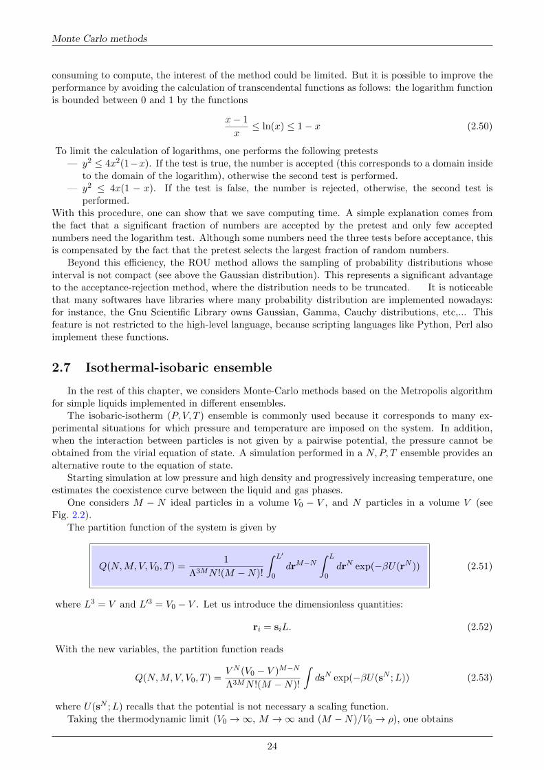
The isobaric-isotherm (P, V, T ) ensemble is commonly used because it corresponds to many ex-perimental situations for which pressure and temperature are imposed on the system. In addition,when the interaction between particles is not given by a pairwise potential, the pressure cannot beobtained from the virial equation of state. A simulation performed in a N,P, T ensemble provides analternative route to the equation of state.
Starting simulation at low pressure and high density and progressively increasing temperature, oneestimates the coexistence curve between the liquid and gas phases.
One considers M − N ideal particles in a volume V0 − V , and N particles in a volume V (seeFig. 2.2).
The partition function of the system is given by
Q(N,M, V, V0, T ) =1
Λ3MN !(M −N)!
∫ L′
0drM−N
∫ L
0drN exp(−βU(rN )) (2.51)
where L3 = V and L′3 = V0 − V . Let us introduce the dimensionless quantities:
ri = siL. (2.52)
With the new variables, the partition function reads
Q(N,M, V, V0, T ) =V N (V0 − V )M−N
Λ3MN !(M −N)!
∫dsN exp(−βU(sN ;L)) (2.53)
where U(sN ;L) recalls that the potential is not necessary a scaling function.Taking the thermodynamic limit (V0 →∞, M →∞ and (M −N)/V0 → ρ), one obtains
24

2.7 Isothermal-isobaric ensemble
V0-VV
Figure 2.2 – Illustration of a simulation using the isothermal-isobaric ensemble. Ideal gas particles arein red, and interacting particles are in blue.
(V0 − V )M−N = VM−N0 (1− V/V0)M−N → VM−N
0 exp(−ρV ). (2.54)
Let us denote that ρ is the density of the ideal gas, the equation is state gives ρ = βP .The system to be studied by simulation is the sub-system consisting of N particles, independently
of ideal gas configurations, which appears in the second box. The partition function of the system ofN particles is then given by using Eq. (2.53)
Q′(N,P, V, T ) = limV0,(M−N)/V0→∞
Q(N,M, V, V0, T )
Qid(M −N,V0, T )(2.55)
where Qid(M−N,V0, T ) is the partition function of a ideal gas of M−N particles occupying a volumeV0, with the temperature T .
By using Eq. (2.54), one obtains
Q′(N,P, V, T ) =V N
Λ3NN !exp(−βPV )
∫dsN exp(−βU(sN ;L)). (2.56)
If the system modifies the volume V , the partition function associated with the subsystem of particlesinteracting with the potential U(rN ) is given by considering the sum of partition functions withdifferent volumes V . This function is then equal to
Q(N,P, T ) =
∫ +∞
0dV (βP )Q′(N,P, V, V0, T ) (2.57)
=
∫ ∞0
dV βPV N exp(−βPV )
Λ3NN !dsN exp(−βU(sN )) (2.58)
The probability P(V, sN ) that N particles occupy a volume V at locations sN is given by
P(V, sN ) ∼ V N exp(−βPV − βU(sN ;L)) (2.59)
∼ exp(−βPV − βU(sN ;L) +N ln(V )). (2.60)
Assuming a detailed balance condition, we choose the transition probabilities of a volume changeaccording to the Metropolis rule.
Π(o→ n) = Min(1, exp(−β[U(sN , Vn)− U(sN , Vo) + P (Vn − Vo)] +N ln(Vn/Vo))
). (2.61)
25

Monte Carlo methods
Unless the interaction potential has a scaling form (U(rN ) = LNU(sN )), volume change is a verydemanding computationally. Attempts to change the volume change are made one time on averagewhen the particles are moved one time on average. For better efficiency, one performs a change ofvariable for a volume by choosing a logarithmic scale instead of a linear scale. As a consequence, thepartition function, (Eq. (2.56)), is expressed as
Q(N,P, T ) =βP
Λ3NN !
∫d ln(V )V N+1 exp(−βPV )
∫dsN exp(−βU(sN ;L)) (2.62)
which gives a modified acceptance rate:
Π(o→ n) = Min(1, exp(−β[U(sN , Vn)− U(sN , Vo) + P (Vn − Vo)] + (N + 1) ln(Vn/Vo))
).
(2.63)
The complete simulation algorithm is as follows:
1. Choose a random integer η between 0 and the total number of particles N .
2. If η 6= 0, select the corresponding particle and perform a trial move within the volumeV of the simulation box. The acceptance probability is given by a standard Metropolisrule.
3. If η = 0, choose a uniform random number between 0 and 1 and calculate the new volumeof the simulation box according to the formula
vn = v0 exp(ln(vmax)(rand− 0.5)). (2.64)
Change the center of mass of each molecule (for point particles, this corresponds tocoordinates) by using the relation
rNn = rNo (vn/vo)1/3 (2.65)
Calculate the energy of the new configuration (a significant computational effort whenthe potential is not simple) and the new configuration is accepted or rejected accordingthe Metropolis rule: (2.61).
2.8 Grand canonical ensemble
The grand-canonical ensemble (µ, V, T ) is suitable for systems in contact with a particle reservoirand a thermostat. This ensemble is appropriate for describing physical situations like isothermaladsorptions (for instance, fluids in zeoliths and other porous media), and for studying the coexistencecurve of fluids.
The system considered here is the sum of a reservoir of ideal gas with M −N particles, placed ina volume V − V0, and of a subsystem of N particles in a volume V0. Instead of changing the volumeas done in the previous section, one exchanges particles.
The partition function reads
Q(M,N, V, V0, T ) =1
Λ3MN !(M −N)!
∫ L′
0drM−N
∫ L
0drN exp(−βU(rN )). (2.66)
Changes of variables are performed with coordinates rN et rM−N are performed as in the previous
26

2.8 Grand canonical ensemble
section, and one finally obtains
Q(M,N, V, V0, T ) =V N (V0 − V )M−N
Λ3MN !(M −N)!
∫dsN exp(−βU(sN )). (2.67)
Taking the thermodynamic limit of an ideal gas reservoir, M →∞, (V0 − V )→∞ with M/(V0 −V )→ ρ, one gets
M !
(V0 − V )N (M −N)!→ ρN . (2.68)
The partition function associated with the subsystem can be expressed as the ratio of partitionfunction of the complete system (Eq. (2.66)) over the subsystem of a ideal gas Qid(M,V0− V, T ) withM particles within a volume V0 − V .
Q′(N,V, T ) = limM,(V0−V )→∞
Q(N,M, V, V0, T )
Qid(M,V0 − V, T )(2.69)
For an ideal gas, the chemical potential is given by the relation
µ = kBT ln(Λ3ρ). (2.70)
In the thermodynamic limit, the partition function of the subsystem defined by the volume V can bewritten as
Q′(µ,N, V, T ) =exp(βµN)V N
Λ3NN !
∫dsN exp(−βU(sN ) (2.71)
Summing over all configurations with a particle number N going from zero to infinity.
Q′(µ, V, T ) = limN→∞
M∑N=0
Q′(N,V, T ) (2.72)
or
Q(µ, V, T ) =
∞∑N=0
exp(βµN)V N
Λ3NN !
∫dsN exp(−βU(sN )). (2.73)
The probability P (µ, sN ) that N particles are in a volume V with coordinates sN is given by
P (µ, sN ) ∼ exp(βµN)V N
Λ3NN !exp(−βU(sN )). (2.74)
Because detailed balance ensures convergence to equilibrium, we choose the transition probabilitiesof a volume change according to the Metropolis rule.
The acceptance rule of the Metropolis algorithm is given by the following equations:
1. For inserting a particle
Π(N → N + 1) = Min
(1,
V
Λ3(N + 1)exp(β(µ− U(N + 1) + U(N)))
). (2.75)
2. For removing a particle
Π(N → N − 1) = Min
(1,
Λ3N
Vexp(−β(µ+ U(N − 1)− U(N)))
). (2.76)
The complete algorithm of a grand-canonical ensemble is made of several steps
27

Monte Carlo methods
1. Choose a random integer η between 1 et N1 with N1 = Nt + nexc (the ratio nexc/〈N〉 sets themean frequency of exchanges with the reservoir) with Nt the particle number in the simulationbox at time t.
2. If η ∈ [1, Nt], choose the corresponding particle and perform a trial move by using the Metropolisrule
3. If η > Nt, select a uniform random number η2 between 0 and 1.
— If η2 < 0.5, one attempts to remove a particle. For that, calculate the energy with theremaining particles Nt−1, and perform the Metropolis test given by equation (2.76). If thenew configuration is accepted, remove the particle. Otherwise, keep the old configuration.
— If η2 > 0.5, one attempts to insert a particle. Calculate the energy with Nt + 1 particlesand one performs the Metropolis test given by equation (2.75). If the new configurationis accepted, add the particle. Otherwise, keep the old configuration.
For very dense fluids, the insertion probability becomes very small and the efficiency of the methoddecreases.
2.9 Liquid-gas transition and coexistence curve
Figure 2.3 – Coexistence curve (temperature versus density) between liquid and gas regions of theLennard-Jones liquid. The dimensionless critical density is close to 0.3 to be compared with thelattice gas model where the dimensionless critical density is 0.5. As expected, the coexistence curveshows an asymmetric shape when decreasing the temperature.
While the study of the phase diagram of lattice models is often restricted to the vicinity of criticalpoints, a complete determination of the phase diagram is often performed for continuous models.This is because, even for a simple liquid, the coexistence curve 4 of liquid-gas displays an asymmetrybetween the liquid region and the gas region, which shows a non universal feature of the system,whereas for a lattice model where a hole-particle symmetry exists, the coexistence curve (temperatureversus density) remains symmetric below the critical density.
When two phases coexist, thermodynamics imposes that temperatures and chemical potentials ofeach phase are equal. A basic idea consists of using an ensemble µ, P, T . Unfortunately, this ensemblecan not defined, because only intensive parameters are involved. A well-defined ensemble requiresat least one extensive variable, either volume or particle number. The method, introduced by Pana-giotopoulos en 1987, is specific for studying the two-phase equilibrium and suppresses the interfacialfree-energy between the two phases, which exists when the two phases are within a simulation box.The presence of a interface between two phases means that one has to overcome a free energy barrier
4. For a liquid, below the critical temperature, it exists a region where liquid and gas phases coexist; boundaries ofthis region defines the coexistence curve.
28

2.10 Gibbs ensemble
in order to go from one phase to one other. The computing time is proportional to the exponential ofthe free energy barrier, and becomes rapidly larger than the simulation time.
2.10 Gibbs ensemble
One considers a system of N particles occupying a volume V = V1+V2, in contact with a thermostatto the temperature T .
The partition function of this system reads
Q(M,V1, V2, T ) =N∑
N1=0
∫ V
0dV1
V N11 (V − V1)N−N1
Λ3NN1!(N −N1)!
∫dsN1
1 exp(−βU(sN11 ))
∫dsN−N1
2 exp(−βU(sN−N12 )).
(2.77)
Comparing this method with the grand canonical method, one notes that particles which occupythe volume V2 are not ideal particles, but they interact with the same potential than particles whichare in the other box.
One easily infers the probability P (N1, V1, sN11 , sN−N1
2 ) of finding a configuration with N1 particlesin the box 1 at the positions sN1
1 and N2 = N −N1 remaining particles in the box 2 at the positionssN2
2 :
P (N1, V1, sN11 , sN−N1
2 ) ∼ V N11 (V − V1)N−N1
N1!(N −N1)!exp(−β(U(sN1
1 ) + U(sN−N12 ))). (2.78)
2.10.1 Acceptance rules
The algorithm involves three kinds of moves: single moves of particles in each box, volume changeswith the constraint that the total volume is conserved, particle swap between boxes.
For single moves within a box, one applies the Metropolis rule for particle displacements like for acanonical ensemble.
For a volume change, a linear scale (Vn = Vo + ∆V ∗ rand) leads to a accpetance rate equal to
Π(o→ n) = Min
(1,
(Vn,1)N1(V − Vn,1)N−N1 exp(−βU(sNn ))
(Vo,1)N1(V − Vo,1)N−N1 exp(−βU(sNo ))
). (2.79)
A logarithmic scale of the volume change is generally more efficient, namely by considering ln(V1/V2),and one obtains an acceptance rate similar to that obtained in the N,P, T ensemble.
Therefore, expressing the partition function by means the logarithmic scale gives:
Q(M,V1, V2, T ) =
N∑N1=0
∫ V
0d ln
(V1
V − V1
)(V − V1)V1
V
V N11 (V − V1)N−N1
Λ3NN1!(N −N1)!∫dsN1
1 exp(−βU(sN11 ))
∫dsN−N1
2 exp(−βU(sN−N12 )). (2.80)
The corresponding probability of volume changes with the logarithmic scale is equal to
p(N1, V1, sN11 , sN−N1
2 ) ∼ V N1+11 (V − V1)N−N1+1
V N1!(N −N1)!exp(−β(U(sN1
1 ) + U(sN−N12 ))) (2.81)
29

Monte Carlo methods
0 0.2 0.4 0.6 0.8 1
X
0
0.2
0.4
0.6
0.8
1
Y
V-V1 N-N
1V
1 N1
Figure 2.4 – Illustration of a simulation using the Gibbs ensemble where the global system is in contactwith a thermostat and where the two sub systems can exchange particles and volume.
and the acceptance rate is then equal to
Π(o→ n) = Min
(1,
(Vn,1)N1+1(V − Vn,1)N−N1+1 exp(−βU(sNn ))
(Vo,1)N1+1(V − Vo,1)N−N1+1 exp(−βU(sNo ))
). (2.82)
The last possibility concerns particle swaps between boxes. For a particle moving from the box 1to the 2, the ratio of the Boltzmann weights is given by
p(o)
p(n)=
N1!(N −N1)!(V1)N1−1(V − V1)N−(N1−1)
(N1 − 1)!(N − (N1 − 1))!(V1)N1(V − V1)N−N1exp(−β(U(sNn )− U(sNo ))
=N1(V − V1)
(N − (N1 − 1))V1exp(−β(U(sNn )− U(sNo ))) (2.83)
which gives
Π(o→ n) = Min
(1,
N1(V − V1)
(N − (N1 − 1))V1exp(−β(U(sNn )− U(sNo )))
). (2.84)
This algorithm is a generalization of the (µ, V, T ) ensemble in which one replaces insertion and removalof particles with particle swap between boxes and in which the volume change, already studied in thealgorithm of the (N,P, T ) ensemble is replaced with a simultaneous volume change of two boxes.
30

3Molecular Dynamics
3.1 Introduction
Monte Carlo simulation has an intrinsic limitation: its dynamics does not correspond to the “real”dynamics. For continuous systems defined from a classical Hamiltonian, it is possible to solve thedifferential equations of all particles simultaneously. This method provides the possibility of preciselyobtaining the dynamical properties (temporal correlations) of equilibrium systems, quantities whichare available in experiments, which allows one to test, for instance, the quality of the model.
The efficient use of new tools is associated with knowledge of their ability; first, we analyze thelargest available physical time as well as the particle numbers that we can consider for a given systemthrough Molecular Dynamics. For a three dimensional system, one can solve the equations of motionfor systems up to several hundred thousands particles. Note that for a simulation with a moderatenumber of particles, namely 104, the average number of particles along an edge of the simulation boxis (104)(1/3) ' 21. This means that for a thermodynamic study one needs to use the periodic boundaryconditions like in Monte Carlo simulations. For atomic systems far from the critical region, thecorrelation length is smaller than the dimensionless length of 21, but Molecular Dynamics is not thebest simulation method for a study of phase transitions. The situation is worse if one considers moresophisticated molecular structures, in particular biological systems.
By using a Lennard-Jones potential, it is possible to find a typical time scale from an analysis ofmicroscopic parameters of the system (m mass of the particle, σ diameter, and ε energy scale of theinteraction potential) is
τ = σ
√m
ε(3.1)
This time corresponds to the duration for a atom of moving on a distance equal to its linear size witha velocity equal to the mean velocity in the liquid. For instance, for argon, one has the numericalvalues σ = 3A, m = 6.63.10−23kg and ε = 1.64.10−20J , which gives τ = 2.8.10−14s. For solving theequations of motion, the integration step must be much smaller than the typical time scale τ , typically∆t = 10−15s, even smaller. The total number of steps performed in a run is typically of order ofmagnitude from 105 to 107; therefore, the duration of the simulation for an atomic system is 10−8s.
For many atomic systems, relaxation times are much smaller than 10−8s and Molecular Dynamicsis a very good tool for investigating dynamic and thermodynamic properties of the systems. For glass-formers, in particular, in for supercooled liquids, one observes relaxation times to the glass transitionwhich increases by several orders of magnitude, where Molecular Dynamics cannot be equilibrated.For conformational changes of proteins, for instance, to the contact of a solid surface, typical relaxationtimes are of order of a millisecond. In these situations, it is necessary to coarse-graining some of themicroscopic degrees of freedom allowing the typical time scale of the simulation to be increased.
31

Molecular Dynamics
3.2 Equations of motion
We consider below the typical example of a Lennard-Jones liquid. Equations of motion of particlei are given by
d2ridt2
= −∑j 6=i∇riu(rij). (3.2)
For simulating an “infinite” system, periodic boundary conditions are used. The calculation of theforce between two particles i and j can be performed by using the minimum image convention (if thepotential decreases sufficiently fast to 0 at large distance. This means that for a given particle i, oneneeds to find if j or one of its images which is the nearest neighbor of i.
Similarly to a Monte Carlo, simulation, force calculation on the particle i involves the computationof de (N − 1) elementary forces between each particle and particle i. By using a truncated potential,one restricts the summation to particles within a sphere whose radius corresponds to the potentialtruncation.In order that the forces remain finite whatever the particle distance, the truncated Lennard-Jones potential used in Molecular Dynamics is the following
utrunc(r) =
u(r)− u(rc) r < rc
0 r ≥ rc.(3.3)
One has to account for the bias introduced in the potential in the thermodynamics quantities comparedto original Lennard-Jones potential.
3.3 Discretization. Verlet algorithm
For obtaining a numerical solution of the equations of motion, it is necessary to discretize. Differentchoices are a priori possible, but as we will see below, it is crucial that the total energy which isconstant for a isolated Hamiltonian system remains conserved along the simulation (let us recall thatthe ensemble is microcanonical). The Verlet’s algorithm is one of first methods and remains one mostused nowadays.
For the sake of simplicity, let us consider an Hamiltonian system with identical N particles. r,is a vector with 3N components: r = (r1, r2, ..., rN , where ri denotes the position of particle i. Thesystem formally evolves as
md2r
dt2= f(r(t)). (3.4)
A time series expansion gives
r(t+ ∆t) = r(t) + v(t)∆t+f(r(t))
2m(∆t)2 +
d3r
dt3(∆t)3 +O((∆t)4) (3.5)
and similarly,
r(t−∆t) = r(t)− v(t)∆t+f(r(t))
2m(∆t)2 − d3r
dt3(∆t)3 +O((∆t)4). (3.6)
Adding these above equations, one obtains
r(t+ ∆t) + r(t−∆t) = 2r(t) +f(r(t))
m(∆t)2 +O((∆t)4). (3.7)
The position updates are performed with an accuracy of (∆t)4. This algorithm does not use theparticle velocities for calculating the new positions. One can however determine these as follows:
v(t) =r(t+ ∆t)− r(t−∆t)
2∆t+O((∆t)2) (3.8)
32

3.3 Discretization. Verlet algorithm
Let us note that most of the computation is spent by the force calculation, and marginally spenton the position updates. As we will see below, we can improve the accuracy of the simulation by usinga higher-order time expansion, but this requires the computation of spatial derivatives of forces andthe computation time increases rapidly compared to the same simulation performed with the Verletalgorithm.
For the Verlet algorithm, the accuracy of trajectories is roughly given by
∆t4Nt (3.9)
where Nt is the total number of integration steps, and the total simulation time is given by ∆tNt.It is worth noting that the computation accuracy decreases with simulation time, due to the
round-off errors which are not included in Eqs. (3.9).There are more sophisticated algorithms involving force derivatives; they improve the short-time
accuracy, but the long-time precision may deteriorate faster than with a Verlet algorithm. In addition,the computation efficiency is significant lower.
Time symmetry is an important property of the equations of motion. Note that Verlet’s algorithmpreserves this symmetry. This is, if we change ∆t→ −∆t, Eq. (3.7) is unchanged. As a consequence, ifat a given time t of the simulation, one inverts the arrow of time , the Molecular Dynamics trajectoriesare retraced. The round-off errors accumulative in the simulation limit the the reversibility when thetotal number of integration steps becomes very large.
For Hamiltonian systems, the volume of phase space is conserved with time, and numerical simu-lation must preserve this property. Conversely, if an algorithm does not have this property, the totalenergy is no longer conserved, even for a short simulation. In order to keep this property, it is necessarythat the Jacobian of the transformation in phase space, namely between the old and new coordinatesin phase space; is equal to one. We will see below that the Verlet algorithm satisfies this property.
An a priori variant of the Verlet algorithm is known as the Leapfrog algorithm and is based onthe following procedure: velocities are calculated on half-time intervals, and positions are obtained oninteger time intervals. Let us define the velocities for t+ ∆t/2 and t−∆t/2
v(t+ ∆t/2) =r(t+ ∆t)− r(t)
∆t, (3.10)
v(t−∆t/2) =r(t)− r(t−∆t)
∆t, (3.11)
one immediately obtainsr(t+ ∆t) = r(t) + v(t+ ∆t/2)∆t (3.12)
and similarlyr(t−∆t) = r(t)− v(t−∆t/2)∆t. (3.13)
By using Eq. (3.7), one gets
v(t+ ∆t/2) = v(t−∆t/2) +f(t)
m∆t+O((∆t)3). (3.14)
Because the Leapfrog algorithm leads to Eq. (3.7), the trajectories are identical to those calculated bythe Verlet’s algorithm. The computations of velocities for half-integer times are temporary variables,but the positions are identical Some care is necessary when calculating the thermodynamics quantitiesbecause the mean potential energy, which is calculated at integer times, and the kinetic energy whichis calculated at half-integer times, do not give a constant total energy.
Many attempts to obtain better algorithms have been made, and, in order to overcome the previousheuristic derivation, a more rigorous approach is necessary. From the Liouville formalism, we aregoing to derive symplectic algorithms, namely algorithms conserving the phase space volume andconsequently the total energy of the system. This method provides algorithms with greater accuracythan the Verlet algorithm for a fixed time step ∆t. Therefore, more precise trajectories can be obtained.
33

Molecular Dynamics
3.4 Symplectic algorithms
3.4.1 Liouville formalism
In the Gibbs formalism, the phase space distribution is given by an N -particle probability distri-bution f (N)(rN ,pN , t) (N is the total number of particles of the system) rN denotes the coordinate setand pN that of the impulses. If f (N)(rN ,pN , t) is known, the average of a macroscopic quantity canbe calculated [29, 11]. By writing the local conservation of the probability distribution, one obtains
∂f (N)(rN ,pN , t)
∂t+
N∑i=1
(∂
∂ri
(dri
dtf (N)(rN , pN , t)
)+
∂
∂pi
(dpi
dtf (N)(rN ,pN , t)
))= 0,
(3.15)
irrespective of the nature of the dynamics. If the dynamics is Hamiltonian(∂HN∂pi
)=vi =
dridt
(3.16)(∂HN∂ri
)=− fi = −dpi
dt. (3.17)
one obtains,
∂
∂ri
(dridt
)= − ∂
∂pi
(dpidt
)(3.18)
which gives the Liouville equation
∂f (N)(rN ,pN , t)
∂t+
N∑i=1
(dridt
∂f (N)
∂ri+dpidt
∂f (N)
∂pi
)= 0, (3.19)
In the following, we only consider Hamiltonian dynamics. The time evolution of the distributionprobability can be expressed as
∂f (N)(rN ,pN , t)
∂t− HN , f (N) = 0, (3.20)
where HN denotes the Hamiltonian of the system of N particles, and the bracket A,B correspondsthe Poisson bracket 1
A,B =
N∑i=1
(∂A
∂ri
∂B
∂pi− ∂B
∂ri
∂A
∂pi
)The Liouville operator is defined as
L = iHN , =N∑i=1
((∂HN∂ri
)∂
∂pi−(∂HN∂pi
)∂
∂ri
)(3.21)
Therefore, Eq. (3.20) is reexpressed as
∂f (N)(rN ,pN , t)
∂t= −iLf (N), (3.22)
1. If A andB are two functions of rN andpN , the Poisson bracket between A andB is defined as
34

3.4 Symplectic algorithms
and one gets the formal solution
f (N)(rN ,pN , t) = exp(−iLt)f (N)(rN ,pN , 0). (3.23)
Similarly, if A is a function of positions rN , and impulses, pN , (but without explicit time dependence)obeys
dA
dt=
N∑i=1
(∂A
∂ri
dridt
+∂A
∂pi
dpidt
). (3.24)
Using the Liouville operator, this equation becomes
dA
dt= iLA, (3.25)
which gives formally
A(rN (t),pN (t)) = exp(iLt)A(rN (0),pN (0)). (3.26)
Unfortunately (or fortunately, because, if not, the world would be too simple), exact expression ofthe exponential operator is not possible in general case. However, one can obtain it in two importantcases: the first expresses the Liouville operator as the sum of two operators
L = Lr + Lp (3.27)
where
iLr =∑i
dridt
∂
∂ri(3.28)
and
iLp =∑i
dpidt
∂
∂pi(3.29)
In a first case, one assumes that the operator Lp is equal to zero. Physically, this corresponds to thesituations where particle impulses are conserved during the evolution of the system and
iL0r =
∑i
dridt
(0)∂
∂ri(3.30)
Time evolution of A(t) is given by
A(r(t),p(t)) = exp(iL0rt)A(r(0),p(0)) (3.31)
Expanding the exponential, one obtains
A(rN (t),pN (t)) = A(rN (0),pN (0)) + iL0rA(rN (0),pN (0)) +
(iL0r)
2
2!A(rN (0),pN (0)) + . . .
=∞∑n=0
∑i
(dridt (0)t
)nn!
(∂n
∂rni
)A(r(0),p(0)) (3.32)
A(rN (t),pN (t)) = A
((ri +
dridt
(0)t
)N,pN (0)
)(3.33)
The solution is a simple translation of spatial coordinates, which corresponds to a free streamingof particles without interaction, as expected.
The second case uses a Liouville operator where L0r = 0. Applying to A, L0
p defined like L0r in the
first case, one obviously obtains the solution of the Liouville equation which corresponds to a simpleimpulse translation.
35

Molecular Dynamics
3.4.2 Discretization of the Liouville equation
In the previous section, we expressed the Liouville operator as the sum of two operators Lr andLp. These two operators do not commute
exp(Lt) 6= exp(Lrt) exp(Lpt). (3.34)
The key point of the reasoning uses the Trotter identity
exp(B + C) = limP→∞
(exp
(B
2P
)exp
(C
P
)exp
(B
2P
))P. (3.35)
For a finite number P of iterations, one obtains
exp(B + C) =
(exp
(B
2P
)exp
(C
P
)exp
(B
2P
))Pexp
(O(
1
P 2
))(3.36)
When truncating after P iterations, the approximation is of order 1/P 2. Therefore, by using ∆t = t/P ,by replacing the formal solution of the Liouville equation by a discretized version, and by introducing
B
P=iLptP
(3.37)
andC
P=iLrtP
, (3.38)
one obtains for an elementary step
eiLp∆t/2eiLr∆teiLp∆t/2. (3.39)
Because the operators Lr and Lp are hermitian, the exponential operator is unitary, and by using theTrotter formula, one gets a method for which we may derive symplectic algorithms namely algorithmspreserving the volume of the phase space.
eiLp∆t/2A(rN (0),pN (0)
)=
A
(rN (0),
(p(0) +
∆t
2
dp(0)
dt
)N) (3.40)
then
eiLr∆tA
(rN (0),
(p(0) +
∆t
2
dp(0)
dt
)N)=
A
(r(0) + ∆tdr(∆t
2 )
dt
)N,
(p(0) +
∆t
2
dp(0)
dt
)N (3.41)
and lastly, applying eiLp∆t/2, we have
A
(r(0) + ∆tdr(∆t
2 )
dt
)N,
(p(0) +
∆t
2
dp(0)
dt+
∆t
2
dp(∆t)
dt
)N (3.42)
In summary, one obtains the global transformations
36

3.5 Hard sphere model
p(∆t) = p(0) +∆t
2(f(r(0)) + f(r(∆t))) (3.43)
r(∆t) = r(0) + ∆tdr(∆t/2)
dt(3.44)
By using Eq. (3.43) with the impulse (defined at half-integer times) and Eq. (3.44) for the initialand final times 0 and −∆t, one removes the velocity dependence and recover the Verlet algorithmat the lowest order expansion of the Trotter formula. Note that it is possible of restarting a newderivation by inverting the roles of operators Lr and Lp in the Trotter formula and to obtains newevolution equations. Once again, the discretized equations of trajectories are those of Verlet algorithm.In summary, the product of the three unitary operators is also a unitary operator which leads to a
symplectic algorithm. In other words, the Jacobian of the transformation, Eq. (3.39), is the productof three Jacobian and is equal to 1. Expansion can be performed to the next order in the Trotterformula: More accurate algorithms can be derived, which are always symplectic, but they involve forcederivatives. Since force calculation is always very demanding, calculation of force derivatives wouldadd a large penalty of the computing performance and are only used when short-time accuracy is acrucial need.
3.5 Hard sphere model
The hard sphere model is defined by the Hamiltonian
HN =
N∑i
(1
2mv2
i + u(ri − rj)
), (3.45)
where the interaction potential is
u(ri − rj) =
+∞ |ri − rj | ≤ σ0 |ri − rj | > σ
(3.46)
From this definition, one sees that the Boltzmann factors, which are involved in the configurationalintegral exp(−βu(ri− rj)) are equal either 0 (when two spheres overlap) or 1 otherwise, which meansthat this integral does not depend on the temperature, but only on the density. As for systems witha purely repulsive interaction, the hard sphere model does not undergo a liquid-gas transition, but aliquid-solid transition exists.
This model was been intensely studied both theoretically and numerically. A renewal of interestin the two last decades comes in the non equilibrium version, commonly used for granular gases.Indeed, when the packing fraction is small, the inelastic hard sphere is a good reference model. Theinteraction potential remains the same, but dissipation that occurring during collisions is accountedfor in a modified collision rule (see Chapter 7).
Note that the impulsive character of forces between particles prevents use of the Verlet algorithmand others; all previous algorithms assume that forces are continuous functions of distance, which isnot the case here.
For hard spheres, particle velocities are only modified during collisions. Between two collisions,particles follow rectilinear trajectories. Moreover, since the collision is instantaneous, the probabilityof having three spheres in contact at the same time is infinitesimal. The dynamics is a sequence ofbinary collisions.
Consider two spheres of identical mass: during the collision, the total momentum is conserved
v1 + v2 = v′1 + v′2 (3.47)
37

Molecular Dynamics
For an elastic collision, the normal component of the velocity at contact is inverted.
(v′2 − v′1).(r2 − r1) = −(v1 − v2).(r2 − r1), (3.48)
whereas the tangential component of the velocity is unchanged.
(v′2 − v′1).n12 = (v1 − v2).n12, (3.49)
where n12 is the normal vector to the collision axis and belonging to the plane defined by the twoincoming velocities.
By using Eqs. (3.48) and (3.49), one obtains the post-collisional velocities
v′1 = v1 +(v2 − v1).(r1 − r2)
(r1 − r2)2(r1 − r2) (3.50)
v′2 = v2 +(v1 − v2).(r1 − r2)
(r1 − r2)2(r1 − r2) (3.51)
It is easy to check that the total kinetic energy is constant during the simulation. Indeed, since thealgorithm being exact (discarding for the moment the round-off problem), the algorithm is obviouslysymplectic.
Practically, the hard sphere algorithm is as follows: starting from an initial (non overlapping)configuration, all possible binary collisions are considered, namely for each pair of particles, collisiontime is calculated.
Between collisions, the positions of i and j are given by
ri = r0i + vit (3.52)
rj = r0j + vjt (3.53)
where = r0i and = r0
i are the particle positions i andj after collision.
The contact condition between two particles is given by relation
σ2 = (ri − ri)2 = (r0
i − r0j )
2 + (vi − vj)2t2 + 2(r0
i − r0j )(vi − vj)t (3.54)
Because the collision time is a solution of a quadratic equation, several cases must be considered: ifthe roots are complex, the collision time is set to a very large value in simulation. If the two roots arereal, either they are negative and the collision time is set to a very large value in simulation again. Ifonly one root is positive, the collision time corresponds to this value. If the two roots are positive, thesmallest one is selected as the collision time.
A necessary condition for having a positive solution for t (collision in the future) is that
(r0i − r0
j ).(vi − vj) < 0 (3.55)
Once all pair of particles have been examined, the shortest time is selected, namely the firstcollision. The trajectories of particles evolve rectilinearly until the new collision occurs (calculation oftrajectories is exact, because forces between particles are only contact forces). At the collision time,velocities of the two particles are updated, and one calculates the next collision again.
The algorithm provides trajectories with an high accuracy, bounded only by the round-off errors.The integration step is not constant, contrary to the Verlet’s algorithm. This quasi-exact method hassome limitation, when the density becomes significant, because the mean time between two collisionsdecreases rapidly and the system then evolves slowly. In addition, rattling effects occur in isolatedregions of the system, which decreases the efficiency of the method.
38

3.6 Molecular Dynamics in other ensembles
3.6 Molecular Dynamics in other ensembles
As discussed above, Molecular Dynamics corresponds to a simulation in the microcanonical en-semble. Generalizations exist in other ensembles, for instance, in canonical ensemble. Let us notethat the thermal bath introduces random forces which changes dynamics with an ad hoc procedure.Because the dynamics then depends on a adjustable parameter, different dynamics can generated thatare different from the “real“ dynamics obtained in a microcanonical ensemble. The methods consistof modifying the equations of motion so that the velocity distribution reaches a Boltzmann distribu-tion. However, this condition is not sufficient for characterizing a canonical ensemble. Therefore, afterintroducing a heuristic method, we will see how to build a more systematic method for performingMolecular Dynamics in generalized ensembles.
3.6.1 Andersen algorithm
The Andersen algorithm is a method where the coupling of the system with a bath is done asfollows: a stochastic process modifies velocities of particles by the presence of instantaneous forces.This mechanism can be interpreted as Monte Carlo-like moves between isoenergy surfaces. Betweenthese stochastic ”collisions”, the system evolves with the usual Newtonian dynamics. The couplingstrength is controlled by the collision frequency denoted by ν. In addition, one assumes that thestochastic “collisions“ are totally uncorrelated, which leads to a Poissonian distribution of collisions,P (ν, t)
P (ν, t) = e−νt (3.56)
Practically, the algorithm is composed of three steps
— The system follows Newtonian dynamics over one or several time steps, denoted ∆t.— On chooses randomly a number of particles for stochastic collisions. The probability of
choosing a particle in a time interval ∆t is ν∆t.— When a particle is selected, its velocity is chosen randomly in a Maxwellian distribution
with a temperature T . Other velocities are not updated.
This procedure ensures that the velocity distribution goes to equilibrium, but obviously, real dy-namics of the system is deeply disturbed. Moreover, the full distribution obtained with the Andersenthermostat is not a canonical distribution: This can be shown by considering the fluctuation calcula-tion. In particular, correlation functions relax at a rate which strongly depends on coupling with thethermostat.
3.6.2 Nose-Hoover algorithm
Refs.[[22, 17]] As discussed above, the Andersen algorithm biases dynamics of the simulation, whichis undesirable, because the main purpose of the Molecular Dynamics is to provide a real dynamics.To overcome this problem, a more systematic approach, introduced by Nose enlarges the system byintroducing additional degrees of freedom. This procedure modifies the Hamiltonian dynamics byadding friction forces which change the particle velocities. These changes increase or decrease thevelocities.
Let us consider the Lagrangian
L =
N∑i=1
mis2
2
(dridt
)2
− U(rN ) +Q
2
(ds
dt
)2
− L
βln(s) (3.57)
where L is a free parameter and U(rN ) is the interaction potential between N particles. Q represent
39
Molecular Dynamics
the effective mass of the unidimensional variable s. The Lagrange equations of this system read
pi =∂L∂ri
= mis2ri (3.58)
ps =∂L∂s
= Qs (3.59)
By using a Legendre transformation, one obtains the Hamiltonian
H =N∑i=1
(pi)2
2mis2+ U(rN ) +
p2s
2Q+L
βln(s) (3.60)
Let us reexpress the microcanonical partition function of this system made of N interacting par-ticles and of this additional degree of freedom interacting with N particles.
Q =1
N !
∫dpsdsdp
NdrNδ(H− E) (3.61)
The partition function corresponds to N indistinguishable particles and to the additional variable inthe microcanonical ensemble where microstates of isoenergy are considered equiprobable.
Let us introduce p′ = p/s. One obtains that
Q =1
N !
∫dpsdss
3Ndp′NdrNδ(
N∑i=1
(p′i)2
2mi+ U(rN ) +
p2s
2Q+L
βln(s)− E) (3.62)
One defines H′ as
H′ =N∑i=1
(p′i)2
2mi+ U(rN ) (3.63)
the partition function becomes
Z =1
N !
∫dpsdss
3Ndp′NdrNδ(H′ + p2
s
2Q+L
βln(s)− E) (3.64)
By using the property
δ(h(s)) =δ(s− s0)
h′(s0)(3.65)
where h(s) is a function with only one zero on the x-axis at the value s = s0. One integrates overthe variable s and one obtains
δ(H′ + p2s
2Q+L
βln(s)− E) =
βs
Lδ(s− exp(−β
L(H′ + p2
s
2Q− E))) (3.66)
This gives for the partition function
Z =β exp(E(3N + 1)/L)
LN !
∫dpsdp
′NdrN exp
(−β(3N + 1)
L(H′ + p2
s
2Q)
)(3.67)
Setting L = 3N + 1, and integrating over the additional degree of freedom, the partially integratedpartition function Q of the microcanonical ensemble of the full system (N particles and the additionaldegree of freedom), becomes a canonical partition function of a system with N particle.
40

3.7 Brownian dynamics
It is worth noting that variables used are r, p′ and ′t′. Discretizing the equations of motion wouldgive a variable time step which is not easy to control in Molecular Dynamics. It is possible to returnto a constant time step by using additional changes of variable. This work was done by Hoover.
Finally, the equations of motion are
ri =pimi
(3.68)
pi = −∂U(rN )
∂ri− ξpi (3.69)
ξ =
(N∑i=1
p2i
2mi− L
β
)1
Q(3.70)
s
s= ξ (3.71)
The two first equations are a closed set of equations for N particles. The last equation controlsthe evolution of the additional degree of freedom in the simulation.
3.7 Brownian dynamics
3.7.1 Different timescales
Until now, we have considered simple systems with a unique microscopic time. For a mixture ofparticles, whose size are very different (an order of magnitude is sufficient, two different microscopictime scales are present (the smallest one is associated with the smallest particles). To obtain thestatistical properties of large particles, simulation time exceeds the computer ability. This situation isnot exceptional, because it corresponds, for instance, to the physical situation of biological moleculesin water. Diluted nanoparticles, like ferrofluids or other colloids, are examples where the presenceof several microscopic timescales prohibits simulation with standard Molecular Dynamics. Browniandynamics (which refers to the Brownian motion) corresponds to a dynamics where smallest particlesare replaced with a continuous media. The basic idea is to perform averages on the degrees of freedomassociated with the smallest relaxation times. Timescales associated with the largest particle movesare assumed larger than the relaxation times of the velocities.
3.7.2 Langevin equation. Discretization
Starting from the Liouville equation of the whole system (large molecules and solvent molecules)and by using a projection method, one obtains a generalized Langevin equation for the variables ofthe large molecules. By using a large time scale separation between the characteristic times associatedwith the solvant and with the large molecules, one obtains equations of motion in terms of Langevinequations.
drN
dt= βDF +
∂
∂rN.D + ξrN (3.72)
where D is the diffusion matrix which depends on the particle configuration in the solvent and ξrN isa Gaussian white noise.
By discretizing the stochastic differential equation, Eq. (3.72) with a constant time step ∆t, oneobtains with a Euler algorithm the following discretized equation
∆rN =
(βDF +
∂
∂rN.D
)∆t+ R (3.73)
41
Molecular Dynamics
∆t is a sufficiently small time step in order that the force changes remain weak in the time step, butsufficiently large for having an equilibrated velocity distribution. R is a random move chosen from aGaussian distribution with a zero mean < R >= 0, and with a variance given by
〈RRT 〉 = 2D∆t (3.74)
RT denotes the transpose of the vector R.A main difficulty with the dynamics is to obtain an expression of the diffusion matrix as a function
of particle configuration. For an infinitely dilute system, the diffusion matrix becomes diagonal andthe nonzero matrix elements are all equal to the diffusion constant in the infinite dilution limit. In ageneral case, the solvent plays a more active role by adding hydrodynamic forces. Theses forces aregenerally long ranged and their effects can not be neglected for modest packing fractions. In the caseof the dilute limit, spherical particles with translational degrees of freedom are involved, the diffusionmatrix has the asymptotic expression
D = D0I +O
(1
r2ij
)(3.75)
with
D0 =1
3πησβ(3.76)
where η is the solvent viscosity, σ is the diameter of the large particles, and β is the inverse of thetemperature. This corresponds to the Stokes law.
3.7.3 Consequences
This stochastic differential equation does not satisfy the time reversal symmetry observed in Hamil-tonian systems. Therefore, the time correlation functions calculated from the Brownian dynamics willbe different on the short time scales. Conversely, one finds glassy behaviors with many studied sys-tems with the Brownian Dynamics. This universal behavior is observed in Molecular Dynamics withmolecular systems (Orthophenyl, salol, glycerol,...) and nanomolecules (ferrofluids, polymers,...).
Let us note that Brownian dynamics which combines aspect of Molecular Dynamics (deterministicforces) and of stochastic process is a intermediate method between Molecular dynamics and MonteCarlo simulation. Optimization techniques and hydrodynamics forces are topics which goes beyondthese lecture notes, but must be considered for efficient and accurate simulation of complex systems.
3.8 Conclusion
The Molecular Dynamics method has developed considerably during these last decades. Initiallydevoted for simulating atomic and molecular systems, generalized ensembles and/or Brownian dynam-ics allow the study of systems containing large molecules, like biological molecules.
42

4Correlation functions
4.1 Introduction
With Monte Carlo or Molecular Dynamics simulation, one can calculate thermodynamic quantities,as seen in previous chapters, but also the spatial correlation functions. These functions characterize thestructure of the system and provide more detailed information that thermodynamic quantities. Corre-lation functions can be directly compared to light or neutron scattering, and/or to several theoreticalapproaches that have been developed during the last decades (for instance, the integral equations ofliquid state). Time correlation functions can be compared to experiments if the simulation dynam-ics corresponds to a ”real” dynamics, namely a Molecular Dynamics. Monte Carlo dynamics stronglydepends of the chosen rule. However, although the Metropolis algorithm does not correspond to a realdynamics, global trends of a real dynamics are generally contained (slowing down for a continuoustransition, glassy behavior in glass formers liquids, ...). Using the linear response theory, the transportcoefficients can be obtained by integrating the time correlation functions.
In the second part of this chapter, we consider the glassy behavior where simulation showedrecently that dynamics of the system is characterized by dynamical heterogeneities. Indeed, whilemany particles seem to be frozen, isolated regions contain mobile particles. This phenomenon evolvescontinuously with time where mobile particles becomes frozen and conversely. This feature can becharacterized by a high-order correlation function (4-point correlation function). Therefore, specificbehavior can be characterized by a more or less sophisticated correlation functions.
4.2 Structure
4.2.1 Radial distribution function
We now derive the equilibrium correlation functions as a function of the local density (alreadydefined in Chap. 1). The main interest is to show that these expression are well adapted for simulation.In addition, we pay special attention to finite size effects; indeed the simulation box containing a finitenumber of particles, quantities of interest display some differences with the same quantities in thethermodynamic limit and one must account for it.
Let us consider a system of N particles defined by the Hamiltonian
H =N∑i=1
p2i
2m+ V (rN ). (4.1)
In the canonical ensemble, the density distribution associated with the probability of finding n particlesin the elementary volume
∏ni=1 dri, denoted in the following as drn, is given by
ρ(n)N (rn) =
N !
(N − n)!
∫. . .∫
exp(−βV (rN ))drN−n
ZN (V, T )(4.2)
43

Correlation functions
where
ZN (V, T ) =
∫. . .
∫exp(−βV (rN ))drN . (4.3)
Normalization of ρ(n)N (rn) is such that∫
. . .
∫ρ
(n)N (rn)drn =
N !
(N − n)!, (4.4)
which corresponds to the number of occurrences of finding n particles among N . In particular, onehas ∫
ρ(1)N (r1)dr1 =N (4.5)∫ ∫ρ
(2)N (r2)dr2 =N(N − 1) (4.6)
which means for Eqs.(4.5) and (4.6) that one can find N particles and one can find N(N − 1) pairsof particles in the total volume, respectively.
The pair distribution function is defined as
g2N (r1, r2) =
ρ(2)N (r1, r2)
(ρ(1)N (r1)ρ
(1)N (r2))
. (4.7)
For an homogeneous system (which is not the case of liquids in the vicinity of interfaces), one
has ρ(1)N (r) = ρ and the pair distribution function only depends on the relative distance between
particles:
g(2)N (r1, r2) = g(|r1 − r2|) =
ρ(2)N (|r1 − r2|)
ρ2(4.8)
where g(r) is called the radial de distribution function.When the distance |r1 − r2| is large, the radial distribution function goes to 1 − 1
N . To thethermodynamics limit, one recovers that the radial distribution function goes to 1, but in finite size,a correction appears which changes the large distance limit.
Noting that
〈δ(r− r1)〉 =1
ZN (V, T )
∫. . .
∫δ(r− r1) exp(−βVN (rN ))drN (4.9)
=1
ZN (V, T )
∫. . .
∫exp(−βVN (r, r2, . . . , rN ))dr2 . . . drN (4.10)
the probability density is reexpressed as
ρ(1)N (r) = 〈
N∑i=1
δ(r− ri)〉. (4.11)
Similarly, one infers
ρ(2)N (r, r′) = 〈
N∑i=1
N∑j=1,j 6=i
δ(r− ri)δ(r′ − rj)〉. (4.12)
By using microscopic densities, the radial distribution function is expressed as
g(2)(r1, r2)ρ(r1))ρ(r2) = 〈N∑i=1
N∑j=1,j 6=i
δ(r− ri)δ(r′ − rj)〉. (4.13)
44

4.2 Structure
0 0.2 0.4 0.6 0.8 1X
0
0.2
0.4
0.6
0.8
1
Y
Figure 4.1 – Basics of the computation of the radial distribution function: starting from a particle,one determines the pair number whose distance is between the successive built from the discretizationgiven by Eq. (4.15).
For a homogeneous and isotropic system, the radial distribution function only depends on themodule of relative distance |r− r′|. Integrating over the volume, one obtains that
ρg(|r|) =1
N〈N∑i=1
N∑j=1,j 6=i
δ(r− ri + rj)〉. (4.14)
In a simulation using periodic boundary conditions (with cubic symmetry), one cannot obtain thestructure of the system beyond a distance equal to L/2, because of the spatial periodicity of each maindirections of the box. Computation of the radial distribution function lies on a space discretization.Practically, one starts with an empty distance histogram of spatial step of ∆r, one calculates thenumber of pairs whose distance is between r and r + ∆r, one performs integration of Eq. (4.14) onthe shell labeled by the index j of thickness ∆r by using the approximate formula:
ρg(∆r(j + 0.5)) =1
N(Vj+1 − Vj)2Np(r), (4.15)
where Np(r) is the number of distinct pairs whose center to center distances are between j∆r and(j + 1)∆r and where Vj = 4π
3 ((j + 1)∆r)3.
This formula is accurate if the radial distribution smoothly varies between the distance r and r+∆r.By decreasing the spatial steps, one can check a posteriori that this condition is satisfied. However, bydecreasing the spatial step of the histogram, the statistical accuracy in each bin diminishes. Therefore,a compromise must be found for the step, based in part on a rule of thumb.
Last, note that computation of this correlation function (for a given configuration) involves all pairs,namely the square of the particle number, a intrinsic property of the correlation function. Because acorrect average needs to consider a sufficient number of different configurations, only configurationswhere all particles have been moved will be considered instead of all configurations. The part ofcomputation time spent for the correlation is then divided by N . In summary, calculation of thecorrelation function scales asN and is comparable to this of the simulation dynamics. The computationtime can be decreased if only the short distance structure is either significant or of interest.
45

Correlation functions
By expressing the radial distribution function with the local density, note that the distributionfunction is then defined in a statistical manner. The ensemble average is not restricted to equilibrium.We will see later (Chapter 7) that it is possible to calculate this function for out of equilibrium systems( random sequential addition) where the process is not described by a Gibbs distribution.
4.2.2 Structure factor
The static structure factor, S(k), is a quantity available experimentally from light or neutronscattering; this is the Fourier transform of the radial distribution function g(r).
For a simple liquid, the static structure factor is defined as
S(k) =1
N〈ρkρ−k〉 (4.16)
where ρk is the Fourier transform of the microscopic density ρ(r). This reads
S(k) =1
N
⟨N∑i=1
N∑j=1
exp(−ikri) exp(ikrj)
⟩. (4.17)
By using δ distributions, S(k) is expressed as
S(k) = 1 +1
N
⟨∫ ∫exp(−ik(r− r′))
N∑i=1
N∑j=1,i 6=j
δ(r− ri)δ(r− rj)drdr′
⟩(4.18)
which gives
S(k) = 1 +1
N
∫ ∫exp(−ik(r− r′))ρ(r, r′)drdr′. (4.19)
For a homogeneous fluid (isotropic and uniform)
S(k) = 1 +ρ2
N
∫ ∫exp(−ik(r− r′))g(r, r′)drdr′ (4.20)
For an isotropic fluid, the radial distribution function only depends on |r− r′|. One then obtains
S(k) = 1 + ρ
∫exp(−ikr)g(r)dr. (4.21)
Because the system is isotropic, the Fourier transform only depends on the modulus k of wave vector,|k|, which gives in three dimensions
S(k) = 1 + 2πρ
∫r2g(r)
∫ π
0exp(−ikr cos(θ)) sin(θ)dθdr (4.22)
and, after some calculation
S(k) = 1 + 4πρ
∫ ∞0
r2g(r)sin(kr)
krdr. (4.23)
Finally, calculation of the static structure factor requires a one-dimensional sine-Fourier transformon the positive axis. Efficient codes of fast Fourier transforms calculate S(k) very rapidly.
In a simulation, one can calculate either g(r) and obtain S(k) by a Fourier transform or S(k) fromEq. (4.17) and obtain g(r) by an inverse Fourier transform. In both cases, knowledge of correlationsis limited to a distance equal to the half length of the simulation box.
46

4.3 Dynamics
For the static structure factor, this yields an infrared cut-off (π/L). The simulation cannot provideinformation for smaller wave vectors. Because the computation of the spatial correlation function overpairs of particles for a given configuration, the number of terms of the summation is proportional to N2
(times the number of configurations used for the average in the simulation). In the direct calculationof the static structure factor S(k), the number of terms to consider is proportional to N multiplied bythe number of wave numbers which are the components of the structure factor (and finally multipliedby the number of configurations used in the simulation.
Repeated evaluation of trigonometric functions in Eq. (4.17) can be avoided by tabulating complexexponentials in an array at the beginning of the simulation
Basically, computation of g(r), followed of the Fourier transform, should give the same resultthan the direct computation of the structure factor. However, because of the finite duration of thesimulation as well as the finite size of the simulation box, statistical errors and round-off errors cangive differences between the two manners of computation.
4.3 Dynamics
4.3.1 Introduction
Spatial correlation functions are relevant probes of the presence or absence of the order at manylenghtscales. Similarly, knowledge of equilibrium fluctuations is provided by time correlation functions.Indeed, let us recall that equilibrium does not mean absence of particle dynamics: the system under-goes continuously fluctuations and how a fluctuation is able to disappear is a essential characteristicassociated with to macroscopic changes, observed in particular in the vicinity of a phase transition.
4.3.2 Time correlation functions
Let us consider two examples of time correlation functions using simple models introduced in thefirst chapter of these lecture notes.
For the Ising model, one defines the spin-spin time correlation function
C(t) =1
N
N∑i=1
< Si(0)Si(t) > (4.24)
where the brackets denote equilibrium average and Si(t) is the spin variable of site i at time t. Thisfunction measures the system looses memory of a configuration at time t. At time t = 0, this functionis equal to 1 (value which can not exceeded, by definition), then decreases and goes to 0 when theelapsed time is much larger than the equilibrium relaxation time.
For a simple liquid made of point particles, one can monitor the density autocorrelation function
C(t) =1
V
∫dr〈δρ(r, t)δρ(r, 0)〉 (4.25)
where δρ(r, t) denotes the local density fluctuation. This autocorrelation function measures theevolution of the local density along the time. It goes to zero when the elapsed time is much larger tothe relaxation times of the system.
4.3.3 Computation of the time correlation function
We now go in details for implementing the time autocorrelation function, for a basic example,namely the spin correlation in the Ising model. This function is defined in Eq. (4.24) 1.
1. Ising model does now own a Hamiltonian dynamics, and must be simulated by a Monte Carlo simulation, but themethod described here can be applied for all sorts of dynamics, Monte Carlo or Molecular Dynamics.
47

Correlation functions
Time average of a correlation function (or others quantities) in the equilibrium simulation (Molec-ular Dynamics or Monte Carlo) is calculated by using a fundamental property of equilibrium systems,namely, time translational invariance: in other words, if one calculates < Si(t
′)Si(t′ + t) >, the re-
sults is independent of t′. In order to have a statistical average well defined, one must iterate thiscomputation for many different t′.
C(t) =1
NM
M∑j=1
N∑i=1
Si(tj)Si(tj + t). (4.26)
where the initial instant is a time where the system is already at equilibrium.We have assumed that the time step is constant. When the later is variable, one can add a constant
time step for the correlation function (in general, slightly smaller than the mean value of variable timestep) and the above method can be then applied.
For practical computation of C(t), one first defined Nc vectors of N components (N is the totalnumber of spins and once equilibrated, one real vector of Nc components and one integer vector of Nc
components. All vectors are initially set to 0.— At t = 0, the spin configuration is stored in the first N component vector, scalar product∑
i Si(t0)Si(t0) is performed and added to the first component of the real Nc component vector— At t = 1, the spin configuration is stored in the second N component vector, scalar products∑
i Si(t1)Si(t1) and∑
i Si(t0)Si(t1) are performed and added to the first and second componentof the real Nc component vector
— For t = k with k < Nc, the same procedure is iterated and k+ 1 scalar products are performedand added in the k + 1 components of the real Nc component vector.
— When t = Nc − 1, the first N component vector is erased and replaced with the new config-uration. NC scalar products can be performed and added to the Nc component vector. Fort = Nc, the second vector is replaced by the new configuration and so on.
— Finally, this procedure is stopped at time t = Tf , and because number of configurations in-volved in averaging the correlation function are not equal, the integer vector of Nc is used as ahistogram of configuration average.
— Finally Eq. (4.26) is used for calculating the correlation function. )A last remark concerns the delicate choice of the time step as well the number of components of the
correlation function. First, the correlation function is calculated for a duration equal to (Nc − 1)∆t,which is bounded
τeq << Nc∆tc << Tsim (4.27)
Indeed, configuration averaging needs that Nc∆tc is less than the total simulation time, but muchlarger than the equilibrium relaxation. Therefore, ∆tc which is a free parameter, is chosen a multipleof the time step of the simulation.
4.3.4 Linear response theory: results and transport coefficients
When a equilibrium system is slightly perturbed by an external field, the linear response theoryprovides the following result: the response of the system and return to equilibrium are directly relatedto the ability of the equilibrium system (namely in the absence of a external field) to answer tofluctuations ( Onsager assumption of fluctuation regression).
In a simulation, it is easier to calculate a correlation function than a linear response functionfor several reasons: i) Computation of a correlation function is done at equilibrium. Practically,the correlation function is obtained simultaneously with other thermodynamic quantities along thesimulation. ii) For computing response functions, it is necessary to perform different simulations foreach response functions. Moreover, for obtaining the linear part of the response function (response of aquantity B(t) to a external field∆F ), one needs to ensure that the ratio 〈∆B(t)〉/∆F is independent of∆F : this constraint leads to choose a small value of ∆F , but if the perturbative field is too weak, thefunction 〈∆B(t)〉 will be small and could be of the same order of magnitude of statistical fluctuationsof the simulation. In the last chapter of these lecture notes, we will introduce a recent method allowing
48
4.3 Dynamics
to calculate response functions without perturbing the system. However, this method is restricted toMonte Carlo simulations. For Molecular Dynamics, fluctuations grow very rapidly with time 2.
In summary, by integrating the correlation function C(t) over time, on obtains the system suscep-tibility.
Consider a system at equilibrium described by the Hamiltonian H0. At time t = 0, this system issubmitted to an external force and the Hamiltonian H′ is given by
H′ = −A(rN )F (t) (4.28)
where F (t) is an external time-dependent force and A(rN ) is the variable conjugate to the force F .One assumes that this force goes to zero when t→∞ such that the system goes to equilibrium. It ispossible to consider a space-dependent force, but for sake of simplicity, we restrict here the analysisto a uniform force.
The time evolution of the system is described by the Liouville equation
∂f (N)(rN ,pN , t)
∂t= −iLf (N)(rN ,pN , t)
=H0 +H′, f (N)(rN ,pN , t)=− iL0f
(N)(rN ,pN , t)− A, f (N)(rN ,pN , t)F (t)
where L0 denotes the Liouville operator associated with H0, L0 = iH0, .Because the system was initially at equilibrium, one has
f (N)(rN ,pN , 0) = C exp(−βH0(rN ,pN )), (4.29)
where C is a normalization constant. Since the external force is weak, one performs a perturbativeexpansion of f (N)(rN ) around equlibrium. One writes
f (N)(rN ,pN , t) = f(N)0 (rN ,pN ) + f
(N)1 (rN ,pN , t) (4.30)
To the lowest order in , one has
∂f(N)1 (rN ,pN , t)
∂t= −iL0f
(N)1 (rN ,pN , t)− A(rN ), f
(N)0 (rN ,pN )F (t). (4.31)
Equation (4.31) is solved formally with the initial condition given by equation (4.29). This gives
f(N)1 (rN ,pN , t) = −
∫ t
−∞exp(−i(t− s)L0)A, f (N)
0 F (s)ds. (4.32)
Therefore, the variable 〈∆B(t)〉 = 〈B(t)〉 − 〈B(−∞)〉 evolves as
〈∆B(t)〉 =
∫ ∫drNdpN
(f (N)(rN ,pN , t)− f (N)
0 (rN ,pN ))B(rN )drNdpN . (4.33)
To lowest order, the difference of Liouville distributions is given by equation (4.32) and equation(4.33) becomes
〈∆B(t)〉 =−∫ ∫
drNdpN∫ t
−∞exp(−i(t− s)L0)A, f (N)
0 B(rN )F (s)ds
=−∫ ∫
drNdpN∫ t
−∞A, f (N)
0 exp(i(t− s)L0)B(rN )F (s)ds (4.34)
2. It exists some cases where the response function is easier to calculate than the correlation function, namely viscosityfor liquids.
49

Correlation functions
by using the fact that the Liouville operator is Hermitian. Calculating the Poisson bracket, oneobtains that
A, f (N)0 =
N∑i=1
(∂A
∂ri
∂f(N)0
dpi− ∂A
∂pi
∂f(N)0
dri
)
=− βN∑i=1
(∂A
∂ri
∂H(N)0
dpi− ∂A
∂pi
∂H(N)0
dri
)f
(N)0
=− βiL0Af(N)0
=− βdA(0)
dtf
(N)0 (4.35)
By inserting equation (4.35) in Eq. (4.34), one obtains
〈∆B(t)〉 = β
∫ ∫drNdpNf
(N)0
∫ t
−∞
dA(0)
dtexp(−i(t− s)L0)B(rN )F (s)ds (4.36)
By using the fact that
B(rN (t)) = exp(itL0)B(rN (0)) (4.37)
Eq. (4.36) becomes
〈∆B(t)〉 = β
∫ t
−∞ds
⟨dA(0)
dtB(t− s)
⟩F (s) (4.38)
One defines the linear response function of B with respect to F as
〈∆B(t)〉 =
∫ ∞−∞
dsχ(t, s)F (s) +O(F 2) (4.39)
With Eq. (4.38), one finds the following properties
1. By equating Eqs. (4.38) and (4.39), one obtains the fluctuation-dissipation theorem
χ(t) =
−βd
dt〈A(0)B(t)〉 t > 0
0 t < 0(4.40)
2. A system cannot respond to a perturbation before it is applied. This property is aconsequence of the causality.
χ(t, s) = 0, t− s ≤ 0 (4.41)
3. The equilibrium response function is translationally invariant in time
χ(t, s) = χ(t− s) (4.42)
When A = B, one denotes the autocorrelation function as
CA(t) = 〈A(0)A(t)〉, (4.43)
and we have
χ(t) =
−βdCA(t)
dtt > 0
0 t < 0(4.44)
50

4.4 Space-time correlation functions
By defining the linear response as
R(t) =
∫ t
0χ(s)ds (4.45)
The fluctuation-dissipation theorem is expressed as
R(t) =
β(CA(0)− CA(t)) t > 0
0 t < 0(4.46)
4.4 Space-time correlation functions
4.4.1 Introduction
To go further in correlation study, one can follow correlations both in space and time. Thisinformation is richer, but the price to pay is the calculation of a two-variable correlation function, atleast. We introduce these functions because they are also available in experiments, essentially formneutron scattering.
4.4.2 Van Hove function
Let us consider the density correlation function which depends both on space and time
ρG(r, r′; t) = 〈ρ(r′ + r, t)ρ(r′, 0)〉 (4.47)
This function can be expressed from the microscopic densities as
ρG(r, r′; t) =
⟨N∑i=1
N∑j=1
δ(r′ + r− ri(t))δ(r− rj(0))
⟩(4.48)
For a homogeneous system, G(r, r′; t) only depends on the relative distance. Integrating over volume,one obtains
G(r, t) =1
N
⟨N∑i=1
N∑j=1
δ(r− ri(t) + rj(0))
⟩(4.49)
At t = 0, the Van Hove function G(r, t) is simplified and one obtains
G(r, 0) =1
N
⟨N∑i=1
N∑j=1
δ(r + ri(0)− rj(0))
⟩= δ(r) + ρg(r) (4.50)
Except a singularity at the origin, at t = 0, the Van Hove function is proportional to the pairdistribution function g(r). On can separate this function in two parts, self and distinct
G(r, t) = Gs(r, t) +Gd(r, t) (4.51)
with
Gs(r, t) =1
N
⟨N∑i=1
δ((r + ri(0)− ri(t))
⟩(4.52)
51

Correlation functions
Gd(r, t) =1
N
⟨N∑i 6=j
δ(r + rj(0)− ri(t))
⟩(4.53)
These correlation functions have the physical interpretation: the Van Hove function is the probabilitydensity of finding a particle i in the vicinity of r at time t knowing that a particle j is in the vicinity ofthe origin at time t = 0. Gs(r, t) is the probability density of finding a particle i at time t knowing thatthis particle was at the origin at time t = 0; finally, Gd(r, t) corresponds to the probability density offinding a particle j different of i at time t knowing that the particle i was at the origin at time t = 0.
Normalization of these two functions reads∫drGs(r, t) = 1 (4.54)
and corresponds to be certain that the particle is in the volume at any time (namely, particle conser-vation).
Similarly, one has ∫drGd(r, t) = N − 1 (4.55)
with the following physical meaning: by integrating over space, the distinct correlation function isable to count the remaining particles.
In the long time limit, the system looses memory of the initial configuration and the correlationfunctions becomes independent of the distance r.
limr→∞
Gs(r, t) = limt→∞
Gs(r, t) '1
V' 0 (4.56)
limr→∞
Gd(r, t) = limt→∞
Gs(r, t) 'N − 1
V' ρ (4.57)
4.4.3 Intermediate scattering function
Instead of considering correlations in space, one can see in reciprocal space, namely in Fouriercomponents. Let us define a correlation function so called intermediate scattering function, which isthe Fourier transform of the Van Hove function
F (k, t) =
∫dkG(r, t)e−ik.rt (4.58)
In a similar manner, one defines self and distinct parts of the function
Fs(k, t) =
∫dkGs(r, t)e
−ikrt (4.59)
Fd(k, t) =
∫dkGd(r, t)e
−ikrt (4.60)
The physical interest of splitting the function is related to the fact that coherent and incoherentneutron scattering provide the total F (k, t) and self Fs(k, t) intermediate scattering functions.
52

4.5 Dynamic heterogeneities
4.4.4 Dynamic structure factor
The dynamics structure factor is defined as the time Fourier transform of the intermediate scat-tering function
S(k, ω) =
∫dtF (k, t)eiωt (4.61)
Obviously, one has the following sum rule: integrating the dynamic structure factor over ω gives thestatic structure factor. ∫
dωS(k, ω) = S(k) (4.62)
4.5 Dynamic heterogeneities
4.5.1 Introduction
In previous sections, we have seen that accurate information how the system evolves by monitoringspace and time correlation functions. However, it exists important physical situations where relevantinformation is not provided by the previous defined functions. Indeed, many systems have relaxationtimes growing in spectacular manner with a rather small variation of a control parameter, namelythe temperature. This corresponds to a glassy behavior, where no significant changes in the structureappear (spatial correlation functions do not change when the control parameter is changes), no phasetransition occurs. Numerical simulations as well experimental results have shown that particles of thesystem, assumed identical, behave very differently at the same time: while most of the particles arecharacterized by a extremely slow evolution, a small part evolves more rapidly. In order to know theseregions have a collective behavior, one needs to build more suitable correlation functions. Indeed, theprevious functions are irrelevant for characterizing this heterogeneous dynamics.
4.5.2 4-point correlation function
The heterogeneities cannot be characterized by a two-point correlation function, but one needs ahigher-order correlation function, and let us define the 4-point correlation function
C4(r, t) = 〈 1
V
∫dr′δρ(r′, 0)δρ(r′, t)δρ(r′ + r, 0)δρ(r′ + r, t)〉
− 〈 1
V
∫dr′δρ(r′, 0)δρ(r′, t)〉〈 1
V
∫dr′δρ(r′ + r, 0)δρ(r′ + r, t)〉 (4.63)
where δρ(r, t) is a density fluctuation at the position r at time t. The physical meaning of this functionis as follows: : when a fluctuation occurs at r′ at time t = 0, how long this heterogeneity will surviveand what is the spatial extension of this heterogeneity?
4.5.3 4-point susceptibility and dynamic correlation length
In order to measure the strength of the correlation defined above, one must perform the spatialintegration of the 4-point correlation function. This defines the 4-point susceptibility
χ4(t) =
∫drC4(r, t) (4.64)
This function can be reexpressed as
χ4(t) = N(< C2(t) > − < C(t) >2) (4.65)
53

Correlation functions
where one defines C(t)
C(t) =1
V
∫drδρ(r, t)δρ(r, 0) (4.66)
as the correlation function (not averaged). For glassy systems, this 4-point susceptibility is a functionwhich displays a maximum at the typical relaxation time. Considering this quantity as algebraic of aquantity ξ(t); this later is interpreted as a dynamic correlation length which characterized the spatialheterogeneities.
4.6 Conclusion
Correlation functions are tools allowing for detailed investigation of spatial and time behavior ofequilibrium systems. As seen above with the 4-point functions, collective properties of systems canbe revealed by building ad hoc correlation functions, when thermodynamic quantities as well as twopoint correlation functions do not change.
54

5Phase transitions
5.1 Introduction
One very interesting application of simulations is to the study of phase transitions, even thoughthey can occur only in infinite systems (namely in the thermodynamic limit). This apparent paradoxcan be resolved as follows: in a continuous phase transition (unlike a first-order transition), fluctuationsoccur at increasing length scales as the temperature approaches the critical point. In a simulationbox, when fluctuations are smaller than the linear dimension of the simulation cell, the system doesnot realize that the simulation cell is finite and its behavior (and the thermodynamic quantities) isclose to an infinite system. When the fluctuations are comparable to the system size, the behaviordiffers from the infinite system close the critical temperature, but the finite size behavior is similar tothe infinite system when the temperature is far from the critical point.
Finite size scaling analysis which involves simulations with different system sizes 1 provides anefficient tool for determining the critical exponents of the system.
Many simulations investigating the critical phenomena (continuous phase transitions) were per-formed with lattice models. Studies of continuous systems are less common. the critical phenomenatheory show that phase transitions are characterized by scaling laws (algebraic laws) whose exponentsare universal quantities independent of a underlying lattice. This is due to the fact that a continuousphase transition is associated with fluctuations of all length scales at the critical point. Therefore,microscopic details are irrelevant in the universal behavior of the system, but the space dimension ofthe system as well as the symmetry group of the order parameter are essential.
Phase transitions are characterized by critical exponents which define universality classes. Studiescan therefore be realized accurately on simple models. For example, the liquid-gas transition for liquidsinteracting with a pairwise potential belongs to the same universality class as the para-ferromagnetictransition of the Ising model.
As we will see below, simulations must be performed with different sizes in order to determine thecritical exponents. If we compare lattice and continuous systems, the former requires less simulationtime. Indeed, varying the size of a continuous system over several orders of magnitude is a challengingproblem, whereas it is possible with lattice systems.
Finally, let us note that the critical temperature obtained in simulations varies weakly with thesystem size in continuous systems, whereas a strong dependence can be observed in lattice models.Consequently, with a modest size, a rather good estimate of the critical temperature can be obtainedwith a simulation.
1. For a good accuracy for the critical exponents, one must choose large simulation cells (and the accuracy of criticalexponents are restricted by the computer powers). Indeed, scaling laws used for the critical exponent calculation corre-sponds to asymptotic behaviors, whose validity is for large simulation cells. To have accurate critical exponents, scalinglaw corrections can be included, which introduces additional parameters to be estimated.
55

Phase transitions
5.2 Scaling laws
5.2.1 Critical exponents
Scaling law assumptions were made in the sixties and were subsequently precisely derived with therenormalization group theory, which provides a general framework for studying critical phenomena.Detailed presentation of this theory goes beyond the scope of these lecture notes, and we only introducethe basic concepts useful for studying phase transitions in simulations
For the sake of simplicity, we consider the Ising model whose Hamiltonian is given by
H = −JN∑
<i,j>
SiSj −HN∑i=1
Si (5.1)
where < i, j > denotes a summation over nearest sites, J is the ferromagnetic interaction strength,and H a uniform external field.
In the vicinity of the critical point (namely, for the Ising model, H = 0, Tc/J = 2.2691 . . . in twodimensions), thermodynamic quantities, as well as spatial correlation functions behave according toscaling laws. The magnetization per spin is defined by
m(t, h) =1
N
N∑i=1
〈Si〉, (5.2)
where t = (T − Tc)/Tc is the dimensionless temperature and h = H/kBT the dimensionless externalfield.
Magnetization (Eq. (5.2)) is defined as
m(t, h) = limN→∞
mN (t, h). (5.3)
In the absence of an external field, the scaling law is
m(t, h = 0) =
0 t > 0
A|t|β t < 0(5.4)
where the exponent β characterizes the spontaneous magnetization in the ferromagnetic phase.Similarly, along the critical isotherm, one has
m(t = 0, h) =
−B|h|1/δ h < 0
B|h|1/δ h > 0(5.5)
where δ is the exponent of the magnetization in the presence of an external field.The specific heat cv is given by
cv(t, h = 0)
C|t|−α t < 0
C ′|t|−α′t > 0
(5.6)
where α and α′ are the exponents associated with the specific heat.Experimentally, one always observes that α = α′. The amplitude ratio C/C ′ is also a universal
quantity. Similarly, one can define a pair of exponents for each quantity for positive or negative
56

5.2 Scaling laws
dimensionless temperature, but exponents are always identical and we only consider an exponent foreach quantity. Isothermal susceptibility in zero external field diverges at the critical point as
χT (h = 0) ∼ |t|−γ , (5.7)
where γ is the susceptibility exponent.
The spatial correlation function, denoted by g(r), behaves in the vicinity of the critical point as
g(r) ∼ exp(−r/ξ)rd−2+η
, (5.8)
where ξ is the correlation length, which behaves as
ξ ∼ |t|−ν , (5.9)
where ν is the exponent associated with the correlation length.
This correlation function decreases algebraically at the critical point as follows
g(r) ∼ 1
rd−2+η(5.10)
where η is the exponent associated with the correlation function.
These six exponents (α, β, γ, δ, ν, η) are not independent! Assuming that the free energy per volumeunit and the pair correlation function obey a scaling function, it can be shown that only two exponentsare independent.
5.2.2 Scaling laws
Landau theory neglects the fluctuations of the order parameter (relevant in the vicinity of thephase transition) and expresses the free energy as an analytical function of the order parameter. Thephase transition theory assumes that the neglected fluctuations of the mean-field approach make anon analytical contribution to the thermodynamic quantities, e.g. the free energy density, denotedfs(t, h):
fs(t, h) = |t|2−αF±f
(h
|t|∆
)(5.11)
where F±f are functions defined below and above the critical temperature and which approach a nonzero value when h→ 0 and have an algebraic behavior when the scaling variable goes to infinity,
F±f (x) ∼ xλ+1, x→∞. (5.12)
Properties of this non analytical term give relations between critical exponents. Therefore, magneti-zation is obtained by taking the derivative of the free energy density with respect to the external fieldh,
m(h, t) = − 1
kBT
∂fs∂h∼ |t|2−α−∆F±
′
f
(h
|t|∆
). (5.13)
For h→ 0, one identifies exponents of the algebraic dependence in temperature:
β = 2− α−∆. (5.14)
57

Phase transitions
Similarly, by taking the second derivative of the free energy density with respect to the field h, oneobtains the isothermal susceptibility
χT (t, h) ∼ t2−α−2∆F±′′
f
(h
|t|∆
). (5.15)
For h→ 0, one identifies exponents of the algebraic dependence in temperature:
− γ = 2− α− 2∆. (5.16)
By eliminating ∆, one obtains a first relation between exponents α, β and γ, called Rushbrookescaling law
α+ 2β + γ = 2. (5.17)
This relation does not depend on the space dimension d. Moreover, one has
∆ = β + γ. (5.18)
Let us consider the limit when t goes to zero when h 6= 0. One then obtains for the magnetization,along the critical isotherm:
m(t, h) ∼|t|β(
h
|t|∆
)λ(5.19)
∼|t|β−∆λhλ. (5.20)
In order to recover Eq. (5.5), magnetization must be finite when t→ 0, i.e. does not diverge or vanish.This yields
β = ∆λ, (5.21)
By identifying exponents of h in Eqs. (5.5) and (5.20) one infers
λ =1
δ. (5.22)
Eliminating ∆ and λ in Eqs. (5.21), (5.22) and (5.18) , one infers the following relation
βδ = β + γ. (5.23)
The next two relations are inferred from the scaling form of the free energy density and of the spatialcorrelation relation g(r). By considering that the relevant macroscopic length scale of the system isthe correlation length, the singular free energy density has the following expansion
fskBT
∼ ξ−d(A+B1
(l1ξ
)+ . . .) (5.24)
where l1 is a microscopic length scale. When t → 0, subdominant corrections can be neglected andone has
fskBT
∼ ξ−d ∼ |t|νd. (5.25)
Taking the second derivative of this equation with respect to the temperature, one obtains for thespecific heat
cv = −T ∂2fs∂T 2
∼ |t|νd−2. (5.26)
58

5.2 Scaling laws
Figure 5.1 – Spin configurations of the Ising model in 2 dimensions: (a) at high temperature. (b) closeto the critical temperature (c) below the critical temperature
By using Eq. (5.6), one infers the Josephson relation (so called the hyper scaling relation),
2− α = dν, (5.27)
which involves the space dimension. Knowing that the space integral of g(r) is proportional to thesusceptibility, one performs the integration of g(r) over a volume whose linear dimension is ξ, whichgives ∫ ξ
0ddrg(r) =
∫ ξ
0ddr
exp(−r/ξ)rd−2+η
(5.28)
With the change of variable u = r/ξ in Eq. (5.28), it comes∫ ξ
0ddrg(r) = ξ2−η
∫ 1
0ddu
exp(−u)
ud−2+η(5.29)
On the right-hand side of Eq. (5.29), the integral is a finite value. By using the relation between thecorrelation length ξ and the dimensionless temperature t (Eq. (5.9)), one obtains that
χT (h = 0) ∼ |t|−(2−η)ν , (5.30)
By considering Eq. (5.7), one infers
γ = (2− η)ν. (5.31)
Finally, since there are four relations between critical exponents that implies only two are indepen-dent 2.
An significant feature of the critical phenomena theory is the existence of a upper and lowercritical dimensions: At the upper critical dimension dsup and above, the mean-field theory (up tosome logarithmic subdominant corrections) describes the critical phase transition. Below lower criticaldimension dinf , no phase transition can occur. For the Ising model, dinf = 1 and dsup = 4. This impliesthat in three-dimensional Euclidean space, a mean-field theory cannot describe accurately the para-ferromagnetic phase transition, in particular the critical exponents. Because the liquid-gas transitionbelongs to the universality class of the Ising model, a similar conclusion applies to the phase transition.
After this brief survey of critical phenomena, we now apply scaling laws for finite size systems todevelop a method which gives the critical exponents of the phase transition as well as non universalquantities in the thermodynamic limit.
2. This property does not apply to quenched disordered systems.
59

Phase transitions
1.8 2 2.2 2.4 2.6 2.8 3T
0
0.2
0.4
0.6
0.8
1
1.2
1.4
1.6
1.8
2
2.2
Cv
L=16L=24L=32L=48
Figure 5.2 – Specific heat versus temperature of the Ising model in two dimensions, The simulationresults correspond to different system sizes where L is the linear dimension of the lattice.
5.3 Finite size scaling analysis
5.3.1 Specific heat
A close examination of spin configuration in Fig. 5.1 merely illustrates that a system close tothe phase transition shows domains of spins of the same sign. The size of domains increases as thetransition is approached. The group renormalization theory showed that, close to the critical point,the thermodynamic quantities of a finite system of linear size L for a dimensionless temperature t,and a dimensionless field h,. . . , are the same of a system of size L/l for a dimensionless temperaturetlyt and a dimensionless field hlyh ,. . . , which gives
fs(t, h, . . . L−1) = l−dfs(tl
yt , hlyh , . . . , (l/L)−1). (5.32)
where yt and yh are the exponents associated with the fields.A phase transition occurs when all variables of fs go to 0. In zero field, one has
fs(t, . . . L−1) = |t|2−αF±f (|t|−ν/L). (5.33)
If the correlation length ξ is smaller than L, the system behaves like an infinite system. But, insimulation, the limit t → 0 can be taken before than L → ∞, and ξ can be larger than L, the lineardimension of the simulation cell; in other words, this corresponds to the fact that the variable of thefunction Ff (Eq. (5.33)) then goes to infinity; this means, one moves away the critical point. Belowand above the critical point of the infinite and for a vicinity which shrinks with increasing sizes ofsimulation cells, the system behaves like an infinite system whereas in the region where the correlationlength is equal to size of the simulation cell, one observes a size-dependence (See Fig. 5.2). If wedenote by Fc the scaling function associated with the specific heat, which depends on the scalingvariable |t|−ν/L, one has
cv(t, L−1) = |t|−αF±c (|t|−ν/L). (5.34)
Because |t|−α goes to infinity when t→ 0, F±c (x) must go to zero when x goes to zero. Reexpressingthis function as
F±c (|t|−ν/L)) = (|t|−ν/L)−κD±(Ltν) (5.35)
60

5.3 Finite size scaling analysis
with D±(0) finite. Since the specific heat does not diverge when |t| goes to zero, one requires that
κ = α/ν (5.36)
which gives for the specific heatcv(t, L
−1) = Lα/νD(L|t|ν). (5.37)
The function D goes to zero when the scaling variable is large and is always finite and positive. D isa continuous function, and displays a maximum for a finite value of the scaling variable, denoted x0.Therefore, for a finite size system, one obtains the following result
— The maximum of the specific heat occurs at a temperature Tc(L) which is shifted withrespect to that of the infinite system
Tc(L)− Tc ∼ L−1/ν . (5.38)
— The maximum of the specific heat of a finite size system L is given by the scaling law
Cv(Tc(L), L−1) ∼ Lα/ν . (5.39)
5.3.2 Other quantities
Similar results can be obtained for other thermodynamic quantities, available in simulations. Forinstance, let us consider the absolute value of the magnetization
〈|m|〉 =1
N〈|
N∑i=1
Si|〉 (5.40)
and the isothermal susceptibility
kBTχ = N(〈m2〉 − 〈m〉2). (5.41)
It is possible to calculate a second susceptibility
kBTχ′ = N(〈m2〉 − 〈|m|〉2) (5.42)
χ increases as N when T → 0, due to the existence of two peaks in the magnetization distributionand does not display a maximum at the transition temperature. Conversely, χ′ goes to 0 when T → 0and has a maximum at the critical point. At high temperature, both susceptibilities are related inthe thermodynamic limit by the relation χ = χ′(1 − 2/π). At the critical point, both susceptibilitiesχ and χ′ diverge with the same exponent, but χ′ has a smaller amplitude.
Another quantity, useful in simulation, is the Binder parameter
U = 1− 〈m4〉3〈m2〉2
(5.43)
The reasoning leading to the scaling function of the specific heat can be used for other thermodynamicquantities and scaling laws for finite size systems are given by the relations
〈|m(t, 0, L−1)|〉 = L−β/νF±m(tL1/ν) (5.44)
kBTχ(t, 0, L−1) = Lγ/νF±χ (tL1/ν) (5.45)
kBTχ′(t, 0, L−1) = Lγ/νF±χ′(tL
1/ν) (5.46)
U(t, 0, L−1) = F±U (tL1/ν) (5.47)
where F±m , F±χ , F±χ′ , and F±U are 8 scaling functions (with different maxima).
61

Phase transitions
Practically, by plotting Binder’s parameter as a function of temperature, all curves U(t, 0, L−1)intersect at the same abscissa (within statistical errors), which determines the critical temperature ofthe system in the thermodynamic limit. Once the temperature of the transition obtained, one cancompute β/ν from 〈|m|〉 , then γ/ν from χ (or χ′). By considering the maximum of Cv or otherquantities, one derives the value of the exponent 1/ν.
Note that in simulation more information is available than the two independent exponents and thecritical temperature. Indeed, because of uncertainty and sub-dominant corrections to scaling laws, 3,by comparing results, one can determine more accurately critical exponents.
Monte Carlo simulation, combined with finite size scaling, is a powerful method for calculatingcritical exponents. Moreover, one also obtains non-universal quantities, like the critical temperature,that no analytical treatment is able to provide with sufficient accuracy until now. Indeed, the renor-malization group can only give critical exponents and is unable to provide a reasonable value of thecritical temperature. Only the functional or non perturbative approach can give quantitative results,but with a high price to pay in terms of computation time.
5.4 Critical slowing down
The nice method, developed in the previous section, uses the idea that the Metropolis algorithmremains efficient even in the vicinity of the critical region. This is not the case, and in order toobtain equilibrium, fluctuations must be sampled at all scales. But, close to the critical point, largescale fluctuations are present and relaxation times increase accordingly; these times are related to thegrowing correlation length by the scaling relation
τ ∼ (ξ(t))z (5.48)
where z is a new exponent, the so-called dynamical exponent. It typically varies between 2 and 5(for a Metropolis algorithm). For a infinite system, knowing that ξ ∼ |t|−ν , the relaxation time thendiverges as
τ ∼ |t|−νz. (5.49)
For a finite-size system, the correlation length is bound by the linear system size L and the relaxationtime increases as
τ ∼ Lz; (5.50)
Simulation times then become prohibitive!
5.5 Reweighting Method
To obtain a complete phase of a given system, a large number of simulations are required forscanning the entire range of temperatures, or for the range of external fields. When one attemptsto locate a phase transition precisely, the number of simulation runs can become prohibitive. Thereweighting method is a powerful techniques that estimates the thermodynamic properties of thesystem by using the simulation data performed at a temperature T , for a set of temperatures between[T −∆T, T + ∆T ] (or for an external field H, within a set of values of the external field [H−∆H,H+∆H]).
The method relies on the following results: Consider the partition function [9, 10, 8],
3. Scaling laws correspond to asymptotic behavior for very large system sizes: in order to increase the accuracy ofthe simulation, one needs to incorporate subdominant corrections.
62

5.5 Reweighting Method
Z(β,N) =∑α
exp(−βH(α))
=∑i=1
g(i) exp(−βE(i)) (5.51)
where α denotes all available states, the index i runs over all available energies of the system, g(i)denotes the density of states of energy E(i). For a given inverse temperature β′ = 1/(kBT
′), thepartition function can be expressed as
Z(β′, N) =∑i
g(i) exp(−β′E(i))
=∑i
g(i) exp(−βE(i)) exp(−(β′ − β)E(i))
=∑i
g(i) exp(−βE(i)) exp(−(∆β)E(i)), (5.52)
where ∆β = (β′ − β).Similarly, a thermal average, like the mean energy, is expressed as:
〈E(β′, N)〉 =
∑i g(i)E(i) exp(−β′E(i))∑i g(i) exp(−β′E(i))
=
∑i g(i)E(i) exp(−βE(i)) exp(−(∆β)E(i))∑i g(i) exp(−βE(i)) exp(−(∆β)E(i))
. (5.53)
In a Monte Carlo simulation, at equilibrium, one can monitor an energy histogram associated withvisited configurations.
This histogram, denoted Dβ(i), is proportional to the density of states g(i) weighted by the Boltz-mann factor,
Dβ(i) = C(β)g(i) exp(−βE(i)) (5.54)
where C(β) is a temperature dependent constant. One can easily see that Eq. (5.53) can bereexpressed as
〈E(β′, N)〉 =
∑iDβ(i)E(i) exp(−(∆β)E(i))∑iDβ(i) exp(−(∆β)E(i))
. (5.55)
An naive (or optimistic) view would consist in believing that a single simulation at given temper-ature could give the thermodynamic quantities of the entire range of temperature 4. As shown in theschematic of Fig. 5.3, when the histogram is reweighted with a lower temperature than the temper-ature of the simulation, (β1 > β), energy histogram is shifted towards to lower energies. Conversely,when reweighted energy histogram with a higher temperature (β2 > β), energy histogram is shiftedtowards the higher energies.
In a Monte Carlo simulation, the number of steps is finite, which means that for a given temper-ature, states of energy significantly lower or larger than the mean energy are weakly sampled, or notsampled at all. Reweighting leads to an exponential increase of errors with the temperature difference.Practically, when the reweighted histogram has a maximum at a distance larger than the standarddeviation of the simulation data, the accuracy of the reweighted histogram, and of the thermodynamicquantities is poor.
We briefly summarize the results of a more refined analysis of the reweighting methodFor a system with a continuous phase transition, the energy histogram Dβ(i) is bell-shaped, and
can be approximated by a Gaussian far from a phase transition. This is associated with the fact that
4. By using a system of small dimensions, one can obtain an estimate for a large range of temperatures.
63

Phase transitions
0 2 4 6 8 10E
0
0.2
0.4
0.6
0.8
1
Dβ(E
)
β1β2
Figure 5.3 – Energy histogram, Dβ(E) of a Monte Carlo simulation (middle curve) to the inversetemperature β; ,Dβ1(E) and Dβ2(E) are obtained by a reweighting method.
at equilibrium, available energy states are around the mean energy value. Far from the critical point,the histogram width corresponds to fluctuations and is then proportional to 1/
√N where N is the site
number or the particle number. This shows that the efficiency of this reweighting method decreaseswhen the system size increases. In the critical region, the width of the energy histogram increases,and if simulation sampling is done correctly, an increasing range of temperatures is estimated by thereweighting method.
In summary, this method is accurate in the vicinity of the temperature of the simulation and allowsone to build a complete phase diagram rapidly, because the number of simulations to perform is quitelimited. By combining several energy histograms (multiple reweighting method), one can improve theestimates of thermodynamic quantities for a large range of temperatures.
The principle of the method developed by considering energy and the conjugate variable β can begeneralized for all pairs of conjugate variables, e.g. the magnetization M and an external uniform fieldH.
5.6 Conclusion
Phase transitions can be studied by simulation, by using several results of statistical physics.Indeed, the renormalization group theory has provided the finite size analysis, which permits theextrapolations of the critical exponents of the system in the thermodynamic limit by using simulationresults of different systems size. Cluster methods are required for decreasing the dynamic exponentassociated with the phase transition. By combining simulation results with a reweighting method, onedrastically reduces the number of simulations. If the accuracy of simulation results are comparableto the theoretical methods for simple systems, like the Ising model, it is superior for almost morecomplicated models.
64

6Advanced Monte Carlo Algorithms
6.1 Introduction
When a system undergoes a continuous phase transition, Monte Carlo methods which consists offlipping (or moving) a single spin (or particle) converge more slowly in the critical region than thecluster algorithm (when it exists). The origin of this slowing down is associated with real physicalphenomena, even if Monte Carlo dynamics can never to be considered as a true dynamics. The rapidincrease of the relaxation time is related to the existence of fluctuations of large sizes (or the presenceof domains) which are difficult to sample by a local dynamics: indeed, cluster algorithms acceleratethe convergence in the critical region, but not far away.
For a first-order transition, the convergence of Monte Carlo methods based on a local dynamics isweak because close to the transition, there exists two or more metastable states: the barriers betweenmetastable states increase with the system size, and the relaxation time has an exponential dependenceof system size which rapidly exceeds a reasonable computing time. Finally, the system is unable toexplore the phase space and is trapped in a metastable region. The replica exchange method provides aefficient way for crossing metastable regions, but this method requires a fine tuning of many parameters(temperatures, exchange frequency between replica).
New approaches have been proposed in the last decade based on the computation of the densityof states. These methods are general in the sense that the details of dynamics are not imposed. Onlya condition similar to the detailed balance is given. The goal of these new methods is to obtain thekey quantity which is the density of states.
6.2 Cluster algorithm
Let us recall that the Metropolis algorithm is a Markovian dynamics for particle motion (or spinflips in lattices). A reasonable acceptance ratio is obtained by choosing a single particle (or spin)in order to have a product |β∆E| which is relatively small. A major advance of twenty years agoconsists of generating methods where a large number of particles (or spins) are moved (or flipped)simultaneously, and keeping a quite high acceptance ratio (or even equal to 1), as well as by reachinga equilibrium state.[27].
We consider below the Ising model, but be generalized the method can be done for all locallysymmetric Hamiltonian (for the Ising model, this corresponds to the up/down symmetry).
Ideally, a global spin flip should have a acceptance ratio equal to 1. The proposed method adds anew step to the Metropolis algorithm: from a given spin configuration, one characterizes the configu-ration by means of bonds between spins. The detailed balance equation (2.17) Chap. 2 is modified asfollows
Pgc(o)W (o→ n)
Pgc(n)W (n→ o)= exp(−β(U(n)− U(o))) (6.1)
where Pgc(o) is the probability of generating a bond configuration from o to n (o and n denote the old
65

Advanced Monte Carlo Algorithms
and new configurations, respectively). If one wishes to accept all new configurations (W (i→ j) = 1),whatever configurations i and j, one must have the following ratio
Pgc(o)
Pgc(n)= exp(−β(U(n)− U(o))) (6.2)
In order to build such an algorithm, let us note that energy is simply expressed as
U = (Na −Np)J (6.3)
where Np is the number of pairs of nearest neighbor spins of the same sign and Na the numberof pairs of nearest neighbor spins of the opposite sign. This formula, beyond its simplicity, has theadvantage of being exact whatever the dimensionality of the system. The method relies on rewritingof the partition function given by Fortuyn and Kasteliyn (1969), but exploiting this idea for simulationoccurred almost twenty years later with the Swendsen and Wang[27] work.
For building clusters, one defines bonds between nearest neighbor spins with the following rules
1. If two nearest neighbor spins have opposite signs, they are not connected.
2. If two nearest neighbor spins have the same sign, they are connected with a probabilityp and disconnected with a probability (1− p).
This rule assumes that J is positive (ferromagnetic system). When J is negative, spins of samesign are always disconnected and spins of opposite signs are connected with a probability p, anddisconnected with a probability (1 − p). Let consider a configuration of Np pairs of spins of samesign, the probability of having nc pairs connected (and consequently nb = Np − nc pairs of spins aredisconnected) is given by the relation
Pgc(o) = pnc(1− p)nb . (6.4)
Once bonds are set, a cluster is a set of spins connected by at least one bond between them. If oneflips a cluster (o → n), the number of bonds between pairs of spins of same and opposite signs ischanged and one has
Np(n) = Np(o) + ∆ (6.5)
and similarly
Na(n) = Na(o)−∆. (6.6)
The energy of the new configuration U(n) is simply related to the energy of the old configurationU(o) by the equation:
U(n) = U(o)− 2J∆. (6.7)
Let us now consider the probability of the inverse process. One wishes to generate the same clusterstructure, but one starts from a configuration where one has Np + ∆ parallel pairs and Na − ∆antiparallel pairs. Antiparallel bonds are assumed broken. One wishes that the bond number n′c isequal to nc because one needs to have the same number of connected bonds for generating the samecluster. The difference with the previous configuration is the number of bonds to break. Indeed, oneobtains
Np(n) = n′c + n′b (6.8)
Np(o) = nc + nb (6.9)
Np(n) = Np(o) + ∆
= nc + nb + ∆, (6.10)
66
6.3 Density of states
which immediately gives
n′b = nb + ∆. (6.11)
The probability of generating the new bond configuration from the old configuration is given by
Pgc(n) = pnc(1− p)nb+∆ (6.12)
Inserting Eqs. (6.4) and(6.12) in Eq. (6.2), one obtains
(1− p)−∆ = exp(2βJ∆) (6.13)
One can solve this equation for p, which gives
(1− p) = exp(−2βJ), (6.14)
Finally, the probability p is given by
p = 1− exp(−2βJ). (6.15)
Therefore, if the probability is chosen according Eq. (6.15), new configuration is always accepted!The virtue of this algorithm is not only its ideal acceptance rate, but one can also show that, in the
vicinity of the critical point, the critical slowing down drastically decreases. For example, the criticalexponent of the two-dimensional Ising model is equal to 2.1 with the Metropolis algorithm while it is0.2 with a cluster algorithm. Therefore, a cluster algorithm becomes quite similar to the Metropolisalgorithm in term of relaxation time far from the critical point.
More generally, Monte Carlo dynamics is accelerated when one finds a method able to flip largeclusters corresponding to the underlying physics. In the Swendsen-Wang method, one selects spinsets which correspond to equilibrium fluctuations; conversely, in a Metropolis method, by choosingrandomly a spin, one generally creates a defect in the bulk of a large fluctuation, and this defect mustdiffuse from the bulk to the cluster surface in order that the system reaches equilibrium. Knowingthat diffusion is like a random walk and that the typical cluster size is comparable to the correlationlength, the relaxation time is then given by τ ∼ ξ2, which gives for a finite size system τ ∼ L2, andexplains why the dynamical exponent is close to 2.
Note that the necessary ingredient for defining a cluster algorithm is the existence of a symmetry.C. Dress et W. Krauth [7] generalized these methods when the symmetry of the Hamiltonian has ageometric origin. For lattice Hamiltonians, where the up-down symmetry does not exist, J. Heringa andH. Blote generalized the Dress and Krauth method by using the discrete symmetry of the lattice [14,15].
6.3 Density of states
6.3.1 Definition and physical meaning
For a classical systems described by a Hamiltonian H, the microcanonical partition function isgiven by (see Chap. 1)
Z(E) =∑α
δ(H− E) (6.16)
where E denotes the energy of the system and the index α runs over all available configurations. Thesymbol δ denotes the Kronecker symbol where the summation is discrete; an analogous formula canbe written for the microcanonical partition function when the energy spectra is continuous; the sumis replaced with an integral and the Kronecker symbol with a δ distribution.
67

Advanced Monte Carlo Algorithms
-2 -1 0 1 2E
0
200
400
600
800
ln(g
(E))
Figure 6.1 – Logarithm of the density of states ln(g(E)) as a function of energy E for a two-dimensionalIsing model on a square lattice of linear size L = 32.
Equation (6.16) means that the microcanonical partition function is a sum over all microstatesof total energy E, each state has a identical weight. Introducing the degeneracy of the system for agiven energy E, the function g(E) is defined as follows: in the case of a continuous energy spectra,g(E)dE is the number of states available of the system for a total energy between E and E+dE. Themicrocanonical partition function is then given as
Z(E) =
∫dug(u)δ(u− E) = g(E) = exp(S(E)) (6.17)
Therefore, the density of states is nothing else than the microcanonical partition function of thesystem and its logarithm is equal to the entropy of the system.
6.3.2 Properties
The integral (or the sum) over all energies of the density of states gives the following rule∫dEg(E) = N (6.18)
where N is the total number of configurations (for a lattice model).For a Ising model, this number N is equal to 2N where N is the total number of spins of the
system. This value is then very large and grows exponentially with the system size. From a numericalpoint of view, one must use the logarithm of this function ln(g(E)) for avoiding overflow problem.
For simple models, one can obtain analytical expressions for small or moderate system sizes, butcombinatorics becomes rapidly a tedious task. Some results can not obtained easily: Indeed, for theIsing model, there are two ground states corresponding to full ordered states. The first nonzero valueof the density of states is equal to 2N which correspond to the number of possibilities of flipping onespin on the lattice of N sites.
Figure (6.1) shows the logarithm of the density of states of the two-dimensional Ising model on asquare lattice with a total number of sites equal to 1024. The shape of this curve is the consequence ofspecific and universal features that we now detail: for all systems where the energy spectra is discrete,the range of energy has a lower bound given by the ground state of the system. In case of simple
68

6.3 Density of states
liquids, the density of states does not have an upper bound, because overlap between particles whichinteract with a Lenard-Jones potential is always possible, which gives very large values of the energy;however the equilibrium probability of having such configurations is weak.
The shape of the curve which displays a maximum is a characteristic of all simple systems, butthe Oy-symmetry is a consequence of the up-down symmetry of the corresponding Hamiltonian. Thissymmetry is also present in thermodynamic quantities, like magnetization versus temperature (seeChapter 1).
For Monte Carlo algorithms based on the density of states, one can simply remark: With theMetropolis algorithm, the acceptance probability of a new configuration satisfies detailed balance,namely Π(i→ j)Peq(i) = Π(j → i)Peq(j) where Peq(j) is the probability of having the configuration jat equilibrium and Π(i→ j is the transition probability of going from the state i towards the state j.One then rewrites detailed balance in energy variable. Let us denote Hβ(E) the energy histogramassociated to successive visits of the simulation. Consequently, one has
Hβ(E) ∝ g(E) exp(−βE) (6.19)
Assume that one imposes the following biased detailed balance
Π(E → E′) exp(−βE + w(E)) = Π(E′ → E) exp(−βE′ + w(E′)) (6.20)
energy histogram then becomes proportional to
Hβ(E) ∝ g(E) exp(−βE + w(E)) (6.21)
It immediately appears that, when w(E) ∼ βE − ln(g(E)), the energy histogram becomes a flathistogram and independent of the temperature. The detailed balance then becomes
Π(E → E′)
g(E)=
Π(E′ → E)
g(E′)(6.22)
The stochastic process corresponds to a random walk in energy space. The convergence of thismethod is related to the fact that the available interval of the walker is bounded. For the Ising model,these bounds exist, for other models, it is possible of restricting the range of the energy interval in asimulation.
This very interesting result is at the origin of multicanonical methods (introduced for the studyof first-order transition). However, it is necessary to know the function w(E), namely to know thefunction g(E). In multicanonical method, a guess for w(E) is provided from the density of statesobtained (by simulation) with small system sizes. By extrapolating an expression for larger systemsizes, the simulation is performed and by checking the deviations of the flatness of the energy histogram,one can correct the weight function, in order to flatten the energy histogram in a second simulationrun.
Performing this kind of procedure consisting of suppressing the free energy barriers which exist in aMetropolis algorithm, and which vanishes here by the introduction of an appropriate weight function.The difficulty of this method is to obtain an good extrapolation of the weight function for large systemsizes. Indeed, a bias of the weight function can insert new free energy barriers and simulations convergeslowly again.
For obtaining a simulation method that computes the density of states without knowledge of agood initial guess, one needs to add an ingredient to the multicanonical algorithm. A new method hasbeen proposed in 2001 by J.S. Wang et D.P. Landau[32, 31], which we detail below.
69

Advanced Monte Carlo Algorithms
6.4 Wang-Landau algorithm
The basics of the algorithm are:
1. A change of the initial configuration is proposed (generally a local modification)
2. One calculates the energy associated with the modified configuration E′. This config-uration is accepted with a Metropolis rule Π(E → E′) = Min(1, g(E)/g(E′)), if notthe configuration is rejected and the old configuration is kept (and added as in an usualMetropolis algorithm)
3. The accepted configuration modifies the density of states as follows: ln(g(E′)) ←ln(g(E′)) + ln(f)
This iterative scheme is repeated until the energy histogram is sufficiently flat: practically, theoriginal algorithm proposes the histogram is flat when each value of the histogram must be largerthan 80% of the mean value of this histogram.
f is called the modification factor. Because the density of states changes continuously in time, itis not a stationary quantity. The accuracy of the density of states depends on the statistical quantityof each value of g(E). Because the density of states increases with time, the asymptotic accuracy isgiven by
√ln(f). To this first stage, the precision is not sufficient for calculating the thermodynamic
quantities.Wang and Landau completed the algorithm as follows: One resets the energy histogram (but,
obviously not the histogram of the density of states). One restart a new simulation described above,but with a new modification factor equal to
√f . Once this second stage achieved, the density of
states is refined with respect to the previous iteration, because the accuracy of the density is given by√ln(f)/2.In order to have an accurate density of states, the simulation is continued by diminishing the
modification factor by the relation
f ←√f (6.23)
When ln(f) ∼ 10−8, the density of states does not longer evolve, the dynamics becomes a randomwalk in energy space and the simulation is then stopped.
Once the density of states obtained, one can easily derive all thermodynamic quantities from thisalone function. A additional virtue in this kind of simulation is that if the accuracy is not reached, thesimulation can be easily prolongated by using the previous density of states until a sufficient accuracyis reached. Contrary to other methods based on one or several values of the temperature, one can herecalculate the thermodynamic quantities for all temperatures (corresponding to the energy scale usedin the simulation).
Considering that the motion in the energy space is purely diffusive (what is only true for the lastiterations of the algorithm, namely values of the modification factor close to one), the computer timewhich is necessary is proportional to (∆E)2, where ∆E represents the energy interval. This meansthat computer time increases as the square of the system size. The computer time of this king ofsimulation is then larger than this of Metropolis algorithm, but for the second case, one obtains thethermodynamic quantities for one temperature (or by using a reweighting method a small interval oftemperature), whereas for only one Wang-Landau simulation, one can obtains these quantities for alarge range of temperatures (as shown below) and the accuracy is much better.
For decreasing the computing time, it is judicious to reduce the energy interval in the simulation,and eventually to perform several simulations for different (overlapping) energy ranges. In the secondcase, the total duration of all simulations is divided by two compared to an unique simulation overthe complete energy space. One can then match the density of states of each simulation. However,this task is subtle, even impossible, if the energy interval belongs to the region of a transition. Indeed,it occurs errors in the density of states at the ends of each density of states forbidding a complete
70

6.5 Thermodynamics recovered!
rebuilding of the density of states. With limitations, the method is very efficient for lattice systemswith discrete energy spectra (additional problems occur with continuous energy spectra. In any case,free energy barriers disappear for first order transition, and it allows for an efficient exploration ofphase space.
6.5 Thermodynamics recovered!
Once obtained the density of states (to an additive constant), one obtains the mean energy (in acanonical ensemble) a posteriori by computing the ratio of following integrals
< E >=
∫E exp(−βE + ln(g(E)))dE∫exp(−βE + ln(g(E)))dE
(6.24)
The practical computation of these integrals requires some caution. The arguments of these expo-nentials can be very large and lead to overflows. For avoiding these problems, let us note that for agiven temperature (or β ), the expression
− βE + ln(g(E)) (6.25)
is a function which admits one or several maxima (but close) and which decreases rapidly towardnegative values when the energy is much smaller or greater to these minima. Without changing theresult, one can multiply each integral by exp(−Max(−βE + ln(g(E)))) 1, the exponentials of eachinterval have an argument always negative or equal to zero. On can then truncate the bounds of eachintegral when the arguments of each exponential become equal to −100 and the computation of eachinterval is safe, without any overflows (or underflows).
The computation of the specific heat is done with the usual formula
Cv = kBβ2(〈E2〉 − 〈E〉2
)(6.26)
It is easy to see that the procedure skechted for the computation of the energy can be transposedidentically for the computation of the specific heat. One can calculate the thermodynamic quantitiesfor any value of the temperature and obtain an accurate estimate of the maximum of the specific heatas well as the associated temperature.
A last main advantage of this method is to obtain the free energy of the system for all temperaturesas well as the entropy of the system, a different situation of a Monte Carlo simulation in the canonicalensemble.
One can also obtain the thermodynamic magnetic quantities with a modest computational effort.Indeed, one obtained the density of states, it is possible to run a simulation where the modificationfactor is equal to 1 (the density of states does not evolve) and therefore the simulation corresponds toa random walk in the space energy: one stores a magnetization histogram M(E) as well as the squaremagnetization M2(E), even higher moments Mn(E).... From these histograms and the density ofstates g(E), one can calculate the mean magnetization of the system as a function of the temperatureby using the following formula
< M(β) >=
∫ M(E)H(E) exp(−βE + ln(g(E)))dE∫
exp(−βE + ln(g(E)))dE(6.27)
and one can obtain the critical exponent associated to the magnetization for a finite size scaling.
Similarly, one can calculate the magnetic susceptibility as a function of the temperature.
1. When there are several maxima, one chooses the maximum which gives the largest value.
71

Advanced Monte Carlo Algorithms
Therefore, one can write a minimal program for studying a system by calculating the quantitiesinvolving the moments of energy in order to determine the region of the phase diagram where thetransition takes place and what is the order of the transition. Secondly, one can calculate otherthermodynamic quantities by performing an additional simulation in which the modification factor isequal to 1. Conversely, for a simulation in a canonical ensemble, a complete program must be writtenfor calculating all quantities from the beginning.
To simply summarize the Monte Carlo simulations based on the density of states, one can say thatan efficient method for obtaining thermodynamics of a system consists in performing a simulationwhere thermodynamics is not involved.
Indeed, simulation is focussed on the density of states which is not a thermodynamic quantity, buta statistical quantity intrinsic of the system.
It is possible to perform simulations of Wang-Landau with a varying number of particles. It allowsone to obtain the thermodynamic potential associated with a grand canonical ensemble. On can alsoperform simulation of simple lquids and build the coexistence curves with accuracu. Let us note thatadditional difficulties occur when the energy spectra is continuous and some refinements with respectto the original algorithm have been proposed by several authors correcting in part the drawbacks ofthe method. Because this method is very recent , improvements are expected in the near future, butthis method represents a breakthough and can alllow studies of systems where standard methods failto obtain reliable thermodynamic quantities. There is an active fied for bringing modifications to theoriginal method (see e.g. the references [34, 23]).
6.6 Monte Carlo method with multiple Markov chains
The free energy barriers prevent the exploration of the phase diagram in a reasonable computertime. The convergence of Metropolis-like algorithms becomes very slow, because the typical relaxationtime is proportional to the exponential of the free energy barriers, which grow with the system size.
To calculate a coexistence curve, or to obtain a well equilibrated system below the critical tem-perature, one has to perform a series of simulations for a sequence of temperature (and/or chemicalpotentials for a liquid)
The “parallel tempering” method (or replica exchange method) is inspired by the following remark:when the temperature decreases, equilibrium is more and more difficult to reach, due to the presenceof large free energy barriers. Conversely, phase diagram is easily explored at high temperatures. Themethod consists of propagating from high temperature toward low temperature configurations andconversely.
For the sake of simplicity, we consider a system where one only changes the temperature, butthe method is easy generalized to other intensive quantities (chemical potential, modification of theHamiltonian,...): the canonical partition function of a system to the temperature Ti is given by therelation
Qi =∑α
exp(−βiU(α)) (6.28)
where α is an index running over all configurations available to the system and βi the inverse of thetemperature.
Let us consider the direct product of all systems evolving to different temperatures, the corre-sponding partition function of this new ensemble is equal to
Qtotal =N∏i=1
Qi (6.29)
where N denotes the total number of temperatures used in all simulation boxes.
72
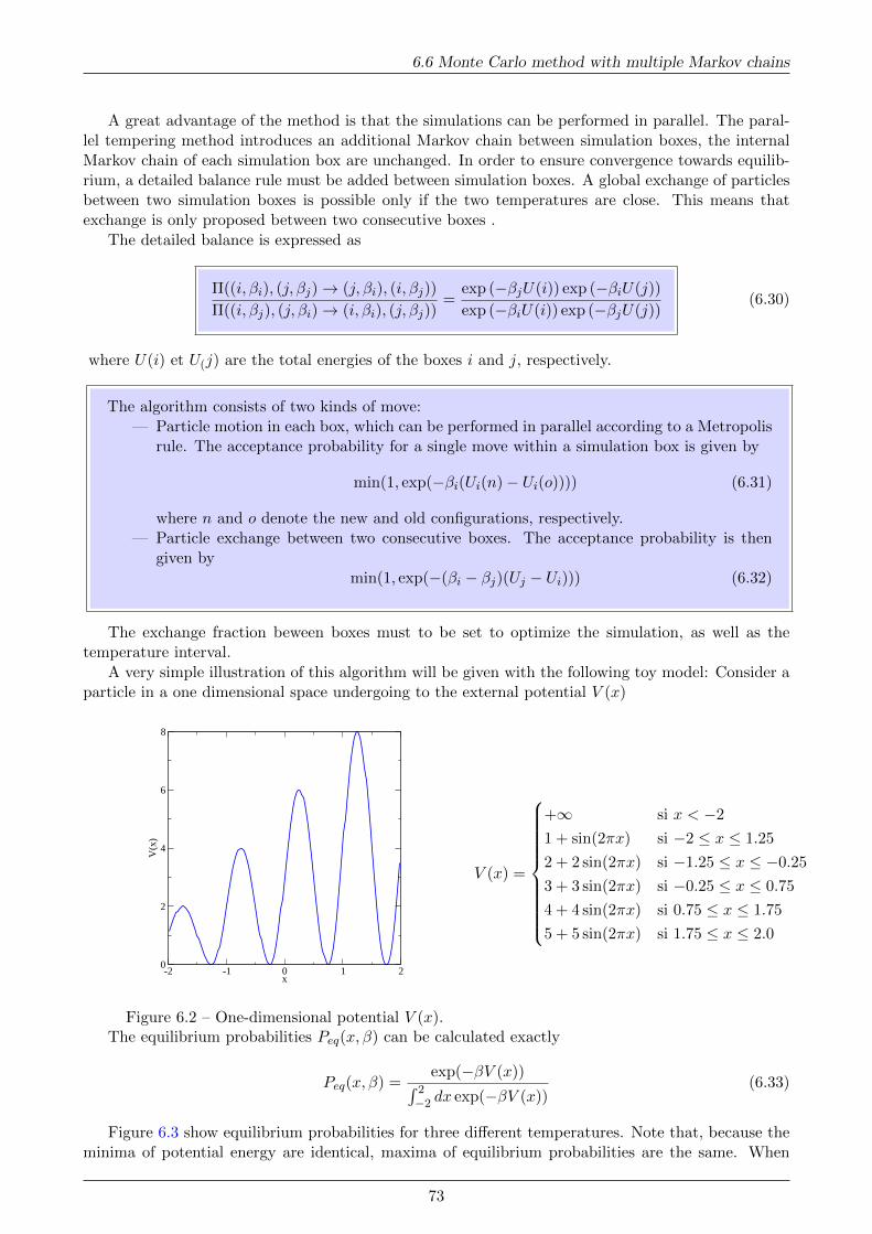
6.6 Monte Carlo method with multiple Markov chains
A great advantage of the method is that the simulations can be performed in parallel. The paral-lel tempering method introduces an additional Markov chain between simulation boxes, the internalMarkov chain of each simulation box are unchanged. In order to ensure convergence towards equilib-rium, a detailed balance rule must be added between simulation boxes. A global exchange of particlesbetween two simulation boxes is possible only if the two temperatures are close. This means thatexchange is only proposed between two consecutive boxes .
The detailed balance is expressed as
Π((i, βi), (j, βj)→ (j, βi), (i, βj))
Π((i, βj), (j, βi)→ (i, βi), (j, βj))=
exp (−βjU(i)) exp (−βiU(j))
exp (−βiU(i)) exp (−βjU(j))(6.30)
where U(i) et U(j) are the total energies of the boxes i and j, respectively.
The algorithm consists of two kinds of move:— Particle motion in each box, which can be performed in parallel according to a Metropolis
rule. The acceptance probability for a single move within a simulation box is given by
min(1, exp(−βi(Ui(n)− Ui(o)))) (6.31)
where n and o denote the new and old configurations, respectively.— Particle exchange between two consecutive boxes. The acceptance probability is then
given bymin(1, exp(−(βi − βj)(Uj − Ui))) (6.32)
The exchange fraction beween boxes must to be set to optimize the simulation, as well as thetemperature interval.
A very simple illustration of this algorithm will be given with the following toy model: Consider aparticle in a one dimensional space undergoing to the external potential V (x)
-2 -1 0 1 2x
0
2
4
6
8
V(x
)
Figure 6.2 – One-dimensional potential V (x).
V (x) =
+∞ si x < −2
1 + sin(2πx) si −2 ≤ x ≤ 1.25
2 + 2 sin(2πx) si −1.25 ≤ x ≤ −0.25
3 + 3 sin(2πx) si −0.25 ≤ x ≤ 0.75
4 + 4 sin(2πx) si 0.75 ≤ x ≤ 1.75
5 + 5 sin(2πx) si 1.75 ≤ x ≤ 2.0
The equilibrium probabilities Peq(x, β) can be calculated exactly
Peq(x, β) =exp(−βV (x))∫ 2
−2 dx exp(−βV (x))(6.33)
Figure 6.3 show equilibrium probabilities for three different temperatures. Note that, because theminima of potential energy are identical, maxima of equilibrium probabilities are the same. When
73

Advanced Monte Carlo Algorithms
the temperature is decreased, the probability of passing between two energy minima becomes verysmall.
-2 -1 0 1 2x
0
0.01
0.02
0.03
0.04
0.05P(
x)
Metropolis+ Exact
-2 -1 0 1 2x
0
0.005
0.01
0.015
0.02
P(x)
Tempering+ Exact
Figure 6.3 – Equilibrium probabilities (full curves) and probabities obtained from simulations forthe particle undergoing to the external one dimensional potential for three different temperaturesT = 0.1, 0.3, 2. (a) Metropolis (b) parallel tempering
Figure 6.3a shows simulation results with a Metropolis algorithm for three different temperatures,whereas figure 6.3b is for a parallel tempering algorithm. The total number of configurations used inboth simulations are the same.
With a Metropolis algorithm, the system is only equilibrated for the highest temperature. ForT = 0.3, the system cannot reach the third potential minimum (knowing that the initial position ofthe particle was in the left region. For T = 0.1, the particle is unable to cross an energy barrier duringthe simulation run. By using the parallel tempering method, the system reaches equilibrium for alltemperatures, in particular even for the lowest temperature.
For an N body system, the parallel tempering algorithm must be performed by using a numberof simulation boxes which increases with the system size. Moreover, this method introduces severalparameters to be set in order that the simulation is efficient: the temperature interval must be set ina subtle manner: if the interval is too large, the acceptance probability for particle exchange is verysmall and the simulation boxes at low temperatures are not sufficiently equilibrated. The temperatureinterval is not necessarily constant (a constant interval in the inverse temperature is more efficient).Once a particle exchange is performed, the system must relax at a given temperature, which meansthat the frequency exchange must be smaller than the inverse of the relaxation time of each simulationbox.
6.7 Conclusion
Monte Carlo methods can be used in various physical situations and can be adapted and/or op-timized by considering the specific properties of a systems to be studied. This chapter is a simpleoverview of a rapidly growing literature, but we hope to give some elements for building more specificmethods.
74

7Stochastic thermodynamics and fluctuation theorems
7.1 Introduction
The classical point of view in thermodynamics is focused on the mean quantities of large systems;indeed, in the thermodynamical limit, the mean quantities per particle are well defined because thefluctuations of these later decrease as long as the central limit theorem holds. In other words, fluctu-ations were considered as a pebble in one’s shoe., and their random behavior seemed to be useless.
Whereas fluctuations have a time evolution which appears stochastic, their statistical propertiesexhibit strong constraints and are the signature of intrinsic properties of the system. A first approachhas revealed this feature through the linear response theory. Basically, at equilibrium, the responseof a system to a small (“infinitesimal”) external field is intimately related to how fluctuations of thequantity (conjugate to the field) vanishes when the system relaxes to equilibrium.
The renewed interest in studying fluctuations is associated with many physical situations wherea thermodynamic limit cannot be taken: for instance, biological systems, colloidal particles drivenby tweezers, biological motors... For these systems, the large molecule undergoes collisions with bathparticles, whose dynamics can be modeled as a stochastic process. Along a trajectory, the large par-ticle exchanges work and heat with its environment in the presence of fluctuations which cannot beneglected. Definitions of thermodynamic quantities have to be adapted to the stochastic dynamics,and this topic is called stochastic thermodynamics. To define these new quantities, we first considerthe trajectories of a particle at a microscopic level surrounded by a environment of small particlesand a external operator able to modify the potential in which the particle evolves. A convenientapproach consists in using a Langevin equation, namely a stochastic differential equation. One firstintroduce some definitions and properties of this mathematical field. Second, two paradigmatic modelsof Langevin are then defined, allowing us to introduce the basic concepts of the stochastic thermody-namics more physically and finally to consider the different fluctuation theorems.
In linear response theory, the role of fluctuations is well understood when the system is close toequilibrium. Several major steps have been done on fluctuations by the findings of different relations,so called fluctuation theorems.
We review some of these results in this chapter, but recent exhaustive reviews[25] and books[26]help readers to go beyond this basic introduction.
7.2 Stochastic differential equations
Let us consider the stochastic differential equation
dx(t)
dt= a(x, t) + b(x, t)ξ(t) (7.1)
75

Stochastic thermodynamics and fluctuation theorems
where ξ(t) is a Gaussian white noise, < ξ(t) >= 0 and < ξ(t)ξ(t′) >= 2δ(t− t′).A formal solution of the stochastic differential equation in the time interval ∆t reads
x(t+ ∆t) = x(t) +
∫ t+∆t
tdt′(a(x, t′) + b(x, t′))ξ(t′) (7.2)
= x(t) +
∫ t+∆t
tdt′a(x, t′) +
∫ t+∆t
tdW (t)b(x, t′) (7.3)
where w(t) is a Wiener process, with dW (t) = ξ(t)dt.
7.2.1 Stochastic calculus
In order to solve the Langevin equation previously introduced, we have to calculate integrals as∫ t
t0
f(t)dW (t) (7.4)
where W (t) is a Wiener process and f(t) an unspecified function A standard way of calculatingthis integral consists of discretizing the time with a constant timestep and performing a Riemannintegration. Therefore, one has
Sn =
n∑i=1
f(τi)(W (ti)−W (ti−1)) (7.5)
where τi is a intermediate time between ti−1 and ti.
By choosing f(t) = W (t), one calculates the average of the integral over all realizations of theWiener process.
< Sn >=
n∑i=1
(Min(τi, ti)−Min(τi, ti−1)) (7.6)
=
n∑i=1
(τi − ti−1) (7.7)
If one chooses τi as the barycenter of the time interval
τi = αti + (1− α)ti−1 (7.8)
with α between 0 and 1, one obtains for the mean value of Sn
< Sn >= α(t− t0) (7.9)
which leads to a result depending on the intermediate point, even after the average over all realization!
For defining the value of a stochastic integral, it is necessary to choose the intermediate point andthe Ito’s choice corresponds to α = 0. Thereforce, one has∫ t
t0
f(t)dW (t) = limn→∞
n∑i=1
f(ti−1)(W (ti)−W (ti−1)) (7.10)
The Ito’s choice corresponds to the fact that the integral is calculated by taking a value of the functionf independent of the behavior of the Wiener process in the future. A principle similar to the causalityprinciple! However, it yields < f(t).dW (t) >=< f(t) >< dW (t) >= 0 and raises question for thecomputation of the work along a stochastic trajectory.
The Stratonovitch’s choice implies that < f(t).dW (t) >6=< f(t) >< dW (t) >6= 0, which leads toadopt this choice in the stochastic thermodynamic.
76

7.3 Langevin dynamics
7.2.2 Change of variable
Let the change of variable dy = f(x(t), t). Performing an expansion to the second order in en dx,one obtains
— Ito calculus
dy(t) = f(x(t+ dt))− f(x(t)) =∂f(x, t)
∂tdt+
∂f(x, t)
∂xdx(t) +
∂2f(x, t)
2∂x2dx(t)2... (7.11)
Using the differential expression of the Langevin equation, the term in dx(t)2 contains termsin dt2, dWdt which can be neglected, but it remains a term dW (t)2 which is in dt to be keept.Therefore, one obtains the following result
dy(t) =
(∂f(x, t)
∂t+ a(x, t)
∂f(x, t)
∂x+∂2f(x, t)
2∂x2b2(x, t)
)dt+ b(x, t)f ′(x).dW (t) (7.12)
— Stratonovitch calculus Let us introduce the Stratonovitch notation, one has
f ′(x) dx = f ′(x+ dx/2)dx
= (f(x) + f ′′(x)dx/2)dx
= df(x) (7.13)
In order to obtain the same trajectory either calculated the Ito calculus and the Stratonovitchcalculus, one uses
b(x, t) dW (t) = b(x, t)dW (t) + b(x, t)∂b(x, t)
∂xdt (7.14)
Finally, the Langevin equation can be expressed as
dx(t) =
(a(x)− b(x, t)∂b(x, t)
∂x
)dt+ b(x) dW (t) (7.15)
Therefore, one can obtain the same trajectory by using the Ito calculus or the Stratonovitch calculus, ifthe Langevin equation is modified as above. Note that when b is independent of x, both equations havethe same expressions. However, when one computes integrals which involves the stochastic variablex(t) (namely work and/or heat, see below), the result depends the choice of Ito or Stratonovitch.
7.3 Langevin dynamics
7.3.1 Underdamped motion
Let us consider a particle in one dimension with an applied force deriving from a potential energyU(x, λ) and in thermal environment, where λ is a parameter which depends on time in general.
dpdt = −∂U(x,λ)
∂x − γ pm + ξ(t)
dxdt = p
m
where ξ(t) is a Gaussian white noise characterized by the two first moments
〈ξ(t)〉 = 0, 〈ξ(t)ξ(t′)〉 = 2γkbTδ(t− t′) (7.16)
and −γ pm is a viscous damping force coming from the thermal environment. In the absence of the
external force, one easily checks that the system obeys the Einstein relation, and leads the system to
equilibrium. It is easy to show that 〈p2
m 〉 = kBT .
77
Stochastic thermodynamics and fluctuation theorems
7.3.2 Overdamped motion
If one assumes that the variation of λ is slow, and the time step ∆t for solving the equationof motion is larger than m/γ, the velocity distribution of the particle is always at equilibrium andthe derivative of the momentum in the Langevin is much smaller than γp/m. The motion is thenoverdamped and the Langevin equation becomes
0 = −∂U(x, λ)
∂x− γ p
m+ ξ(t) (7.17)
which can be reexpressed asdx
dt=
1
γ
(−∂U(x, λ)
∂x+ ξ(t)
)(7.18)
7.4 Fokker-Planck and Kramers equations
Whereas the Langevin equation is well adapted for obtaining information for a single trajectory,the Fokker-Planck and Kramers equation describe the evolution of the probability P (x, p, t) whichcorresponds to an average over a large number of trajectories.
For underdamped motion, one has
∂P (x, p, t)
∂t=
[− p
m
∂
∂x+
∂
∂p
(∂U(x, λ)
∂x+ γ
p
m
)+
∂2
∂p2γkBT
]P (x, p, t) (7.19)
Note that the Kramers equation can be interpreted as an equation of continuity in the phase space
∂P (x, p, t)
∂t= −∂Jx
∂x− ∂Jp
∂p= −~∇. ~J (7.20)
with
~J =
Jx = p
mP (x, p, t)
Jp =(−∂U(x,λ)
∂x − γ pm
)− ∂
∂p(γkBTP (x, p, t))(7.21)
is the flux of probability at point (x, p).Note that when λ and T are constant, the Kramers equation converges equilibrium.
Peq(x, p) =exp
(−β(p2
2m + U(x, λ)))
√2πm/β
∫dx exp
(−β(p2
2m + U(x, λ))) (7.22)
For an overdamped motion, the velocity distribution is at equilibrium all the time and the positiondistribution obeys the Fokker-Planck equation
∂P (x, t)
∂t= − ∂
∂x
(1
γ
[∂U(x, λ)
∂x+
∂
∂xkBT
])P (x, t) = −∂J
∂x(7.23)
where J is the probability flux
J =1
γ
(∂U(x, λ
∂x+
∂
∂xkBT
)P (x, p, t) (7.24)
78

7.5 Path integral approach
Is is worth noting that the position distribution also reaches equilibrium for long time.
Peq(x) =exp (−βU(x, λ))∫dx exp (−βU(x, λ))
(7.25)
7.5 Path integral approach
A third approach for the stochastic processes can be done by using the formalism of path ensemble.ξ(t) is a Gaussian white noise, with the two first moments 〈ξ(t)〉 = 0 and 〈ξ(t)ξ(t′)〉 = 2γkbT . Theprobability of having a path ξ(t) between 0 and t is given by
P [ξ] ∝ exp
(− 1
4γkBT
∫ t
0du ξ2(t)
)(7.26)
For an overdamped motion, the Langevin equation can be expressed as
γdx
dt+∂U(x, λ)
∂x= ξ(t) (7.27)
which can be interpreted as follows: when one solves the stochastic differential equation: the noiseis converted in position fluctuations of the particle. Therefore, the probability of having a trajectoryx(t) is given by
P [x] ∝ exp
(− 1
4γkBT
∫ t
0du
[γdx
dt+∂U
∂x
]2
− 2kBT∂2U
∂x2
)(7.28)
The seconde derivative of the potential in Eq.7.28 comes from the Jacobian of the change of variableξ(t) to x(t). Indeed, taking a finite time step, the Langevin equation is expressed as
γ((xn+1 − xn) = −1
2(U ′(xn+1)− U ′(xn))δt+
√2γkBT (Wn+1 −Wn) (7.29)
Note that a trapezoidal rule is used. The Jacobian of the elementary transformation is then equal to
∂(Wn+1 −Wn)
∂(xn+1 − xn)=
γ√2γkBT
(1 +δt
2γU ′′(xn) (7.30)
Finally, one takes the limit ∆t→ 0, and one obtains
t∆t∏n=0
(1 +δt
2γU ′′(xn))→ exp
(1
2γ
∫ t
0U ′′(x)ds
)(7.31)
Contrary to Hamiltonian systems, the Langevin equation breaks the time-reversal symmetry. How-ever, one can see that the time-reversal process ξ(−t) occurs with the same probability. When aLangevin process described a motion at equilibrium, the probability of having the time-reversal tra-jectory x(−t) is equal to the probability of having x(t). This symmetry is called detailed balance.Consequently, no work can be extracted from the stochastic motion of the particle, corresponding tothe prescription of the second law of thermuodynamics.
79

Stochastic thermodynamics and fluctuation theorems
System
Reservoir External
d'Wd'Q
dE
Figure 7.1 – Scheme of the energy fluxes between the three parts of the world. The arrows indicatepositive fluxes.
7.6 Stochastic thermodynamics
In order to define the fluctuating thermodynamic quantities of a stochastic process, one first definesthe world consists in three parts: the system, the thermal environnement and the external operator.(See Fig. (7.1) Afin de definir les quantites thermodynamiques fluctuantes d’un processus stochastique,on definit tout d’abord le monde constitue de trois parties: le systeme, l’environnement thermique etun operateur externe. (Voir Fig. (7.1))
As for macroscopic systems, when the system receives heat from the reservoir (thermal environ-ment), it is considered as positive. For an infinitesimal timestep dt. The force exerced by the thermalenvironment is −γ dxdt + ξ(t) and the heat received is d′Q
d′Q =
(−γ dx
dt+ ξ(t)
) dx(t) (7.32)
Note that the product is performed by the Stratonovitch rule for physical reasons.
For an underdamed motion, the heat is slightly modified by replacing dxdt with the momentum p.
Moreover, by using the equation of motion, one obtains
d′Q =
(dp
dt+∂U(x, λ)
∂x
) dx(t) (7.33)
7.6.1 First law of thermodynamics
The work brought to the system corresponds to a change performed by the external operator, onehas
d′W =∂U(x, λ)
∂λ dλ(t) (7.34)
For a underdamped motion, one uses two identities
dp
dt dx(t) =
dp
dt pmdt = d
(p2
2m
)∂U(x, λ)
∂x dx(t) = dU(x(t), λ(t))− ∂U(x, λ)
∂λ dλ(t)
which gives
dE = d′Q+ d′W (7.35)
80

7.6 Stochastic thermodynamics
where E is the total energy of the system
E =
(p2
2m+ U(x, λ)
)(7.36)
Eq.(7.35) expresses the conservation of the energy of the system.
For an overdamped motion, by using the Langevin equation and Eq.(7.32), the heat is given by
d′Q =∂U(x, λ)
∂x dx(t) (7.37)
and one immediately obtains
dU(x, λ) = d′Q+ d′W (7.38)
Because the motion is overdamped, the mean kinetic energy stays at equilibrium and only the internalenergy is modified when work and/or heat are brought to the system. Comme le mouvement estsuramorti, l’energie cinetique moyenne reste a l’equilibre et seule l’energie interne est modifiee quanddu travail ou de la chaleur sont apportes au systeme.
The thermodynamics quantities have been defined for a single trajectory, and it is also interestingto calculate an ensemble average of these fluctuating observables. It is convenient to use the Fokker-Planck and/or Kramers equations.
For a underdamped motion, the mean heat variation is given by
〈d′Q〉 =
∫ (∂E
∂xJx +
∂E
∂pJp
)dxdp (7.39)
~J is the flux of probability in the phase space. Similarly, for an overdamped motion, one has
〈d′Q〉 =
∫∂E
∂xJxdx (7.40)
7.6.2 Entropy and second law of thermodynamics
It is now possible to define a stochastic entropy which comes from the particle trajectory
s(t) = − ln(p((xt, λ), t)) (7.41)
where p((xt, λ), t) is the probability provided by the Fokker-Planck equation associated with theLangevin equation and calculated along the particle trajectory xt. As a consequence, the stochas-tic entropy depends both on the trajectory and on the ensemble. Taking the time derivative of thestochastic entropy, one has
ds(t)
dt= −∂tp(x, t)
p(x, t)− ∂xp(x, t)
p(x, t)
dx
dt(7.42)
By using Eq.(7.24)
∂xp(x, t) = β(γJ(x, t) + ∂xU(x, t)p(x, t)) (7.43)
one obtainsds(t)
dt= −∂tp(x, t)
p(x, t)+
(βγJ(x, t)
p(x, t)+ β∂xU(x, t)
)xt
dx
dt(7.44)
81

Stochastic thermodynamics and fluctuation theorems
It is possible to calculate the entropy dissipated into the environment: the heat released in theenvironnement is equal to the opposite heat received by the system and the entropie rate is given by
dsm(x(t))
dt= β−dq(x(t))
dt(7.45)
By using Eq.(7.37)dsm(x(t))
dt= −β∂xU(x, t)
dx
dt(7.46)
By summing the two entropies, one obtains the total entropy
dstot(t)
dt= −∂tp(x, t)
p(x, t)+
(J(x, t)
Dp(x, t)
)xt
dx
dt(7.47)
where D = T/γ. The total entropy only increases by averaging over all trajectoiries. By using thefollowing result ⟨
g(x)dx
dt
⟩=
∫dxg(x)j(x, t) (7.48)
one obtains
dStot(t)
dt=
⟨dstot(t)
dt
⟩=
∫dx
j2(x, t)
Dp(x, t)=< v2(x, t) >
D≥ 0 (7.49)
Therefore, one recovers that the total entropy increases with time as the second law of the thermody-namics predicts.
7.7 Classification
The different fluctuation theorems express the universal properties of the probability distribution ofthe thermodynamic quantities. This corresponds to a generalisation of thermodynamics by includingthe fluctuations. Three classes of properties have been proved under specific assumptions. Let usintroduce a variable Λ(x, t) which depends on x and t.
7.7.1 Integral fluctuation theorem
If Λ(x, t) is a non dimensional functional, one says that Λ obeys the integral fluctuation theoremiff
〈exp(−Λ)〉 =
∫dΛp(Λ) exp(−Λ) = 1 (7.50)
where p(Λ) is the distribution probability.
Several properties can be infered from the IFT
—
〈Λ〉 ≥ 0 (7.51)
which is a consequence of the convexity of the exponential function.— The integral being equal to 1, there are trajectories where Λ is negative. There is an apparent
violation of the second law of thermodynamics. In fact, this corresponds to fluctuations whichcan lead to negative values of Λ.
—
P (Λ < −λ) ≤∫ −λ−∞
dΛp(Λ)e−λ−Λ ≤ e−λ (7.52)
82

7.8 Work fluctuation theorems
To prove the inequality, one writes
P (Λ < −λ) =
∫ −λ−∞
dΛp(Λ)
≤∫ −λ−∞
dΛp(Λ)e−λ−Λ
≤∫ ∞−∞
dΛp(Λ)e−λe−Λ
≤ e−λ (7.53)
— IFT imposes a constraint between the variance and the mean of Λ
〈(Λ− 〈Λ〉)2〉 = 2〈Λ〉 (7.54)
7.7.2 Detailed fluctuation theorem
The detailed fluctuation theorem provides a relation between the probability of obtaining thequantity Λ and the opposite −Λ:
p(−Λ)
p(Λ)= exp(−Λ) (7.55)
Several properties can be also infered from this theorem
When a quantity Λ satisfies this relation, the IFT is also satisfied.∫dΛ exp(−Λ)p(Λ) =
∫dΛp(−Λ) (7.56)
=
∫dΛp(Λ) = 1 (7.57)
7.7.3 Generalized Crooks fluctuation theorem
The generalized Crooks fluctuation theorem provides a relation comparing the probability distri-bution function p(Λ) with the probability p†(Λ) of the same quantity Λ for a “conjugate” process(generally one considers a time-reversed process)
p†(−Λ)
p(Λ)= exp(−Λ) (7.58)
7.8 Work fluctuation theorems
We first consider work fluctuations when the initial configuration is in equilibrium whereas thefinal configuration is not necessarily in equilibrium. The system evolves between the two states dueto a driving force.
7.8.1 Jarzynski relation
Jarzynski showed the work which allows to drive the system from the initial equilibrium state byusing a time-dependent potential V (x, λ) for a time t satisfies the relation⟨
exp(−wT
)⟩= exp
(−∆F
T
)(7.59)
83

Stochastic thermodynamics and fluctuation theorems
where ∆F is the difference of the free energy between the final state where the control parameter isequal to λt and the initial state with a control parameter λ0. This can be viewed as a IFT relationfor the dimensionless dissipated work.
wd =w −∆F
T(7.60)
Therefore, experimentally and/or in simulation, it becomes possible to obtain the free energy difference∆F = F(λt)−F(λ0), namely a equilibrium property, from non equilibrium measurements.
7.8.2 Crooks fluctuation theorem
The Crooks fluctuation theorem states that the probability distribution p(w) for work spent inthe process is related to the probability distribution p for work in the reverse process. The controlparameter of the reversed process is given by λ(τ) = λ(t − τ) and the initial state of the reversedprocess is an equilibrium state where λ(0) = λ(t).
p(w)
p(w)= exp
(−w −∆F
T
)(7.61)
Note that for a system where the Crooks relation holds, the Jarzynski theorem is satisfied. Indeed,knowing that p(w) is normalized, one immediately infers that the JR holds.
7.9 Entropy production
The entropy production along a trajectory is the sum of two terms as previously seen
∆stot = ∆sm + ∆s (7.62)
with∆s = − ln(p(xt, λt)) + ln(p(x0, λ0)) (7.63)
The total entropy obeys the IFT〈exp (−∆stot)〉 = 1 (7.64)
By using the convexity of the exponential function, one infers that 〈∆stot〉 ≥ 0 wich shows that theentropy production is obviously compatible with the second law of thermodynamics.
7.10 Conclusion
The research on Fluctuation theorems is a very active field under progress: new results are foundcontinously. Applications of these findings concern interdisciplinary fields, as biology, nanotechnologyallowing to obtain deeper understanding of phenomena, which are in non equilibrium situations. Sim-ulations and theoretical approaches of paradigmatic provide precise results benchmarking new ideasin this field.
84

8Out of equilibrium systems
8.1 Introduction
In the two following chapters, we consider the large domain of out-of-equilibrium statistical physics.Physical situations where a system evolves without reaching equilibrium are very frequent. There aredifferent reasons: i) a system is not isolated, for instance in contact with a thermostat, or surroundedby several particle reservoirs,... which prevents to reach equilibrium; ii) the relaxation times may bemuch larger than the typical experiment time, and the system cannot reach equilibrium (for instance,protein adsorption at liquid-solid interfaces, polymers, glassformers, spin glasses); iii) The system hasan intrinsic irreversibility (for instance, collisional dynamics for granular matter) for which one needsto introduce an appropriate out of equilibrium statistical description (granular matter, fragmentation,growing phenomena, avalanches, earthquakes)[30, 16, 28].
These systems can be separated in three large classes which describe their out of equilibrium evolu-tion: First, relaxation times are very large (significantly larger than the experimental time), second, theevolution is driven towards non equilibrium states. Lastly, systems evolve under external constraintstowards stationary states, with a microscopic dynamics that may or may not be Hamiltonian.
The relevance of this approach is illustrated by considering several toy models of non equilibriumstatistical physics. Special attention will be devoted to algorithms of numerical simulation of thesesystems.
A numerical approach is justified by the absence of a general theoretical framework of out-of-equilibrium systems. Numerical results allow us to understand the physics of such systems and are anefficient tool for developing theoretical methods.
8.2 Random sequential addition
8.2.1 Motivation
When a solution of macromolecules (proteins, colloids) is placed in contact with a solid surface, oneobserves a surface adsorption as a monolayer of macromolecules. This process is slow; the adsorptioncan take from several minutes to several weeks. Once adsorption performed, if one replaces thesolution with a buffer solution, little or no desorption is observed and there are few changes in thestructure of the adsorbed monolayer. When the experiment is repeated with different concentrationsof macromolecules, the saturation coverage is always the same[28].
Considering the typical time scales and the microscopic complexity of molecules, it is not possibleto perform Molecular Dynamics describing the process. A first step consists of coarse-graining thesystem with a “mesoscopic” length scale. The typical size of molecules is from 10nm to some mm,and therefore the range of interaction between particles is smaller than the particle size. The shape ofthese particles does not change during the process and particles cannot overlap. As a first approach,the interaction potential can be taken as a hard core potential (for instance for colloids).
85
Out of equilibrium systems
When the particle is in the neighborhood of the surface, the interaction with the surface is stronglyattractive on a short distance and strongly repulsive when the particle goes into the surface. The in-teraction potential can be approximated as a strongly attractive contact potential. Once adsorbed,particles cannot desorb or move on the surface. Because particles in solution follow Brownian trajecto-ries, one can assume that particles reach the surface randomly. If the particle first reaches an adsorbedparticle, it is pushed away from the surface and returns to the bulk. If the particle reaches the solidsurface, without overlapping other adsorbed particles, it is “glued” to the surface, definitively.
8.2.2 Definition
Once the system has been coarse-grained, the particle adsorption can be described by the followingmodel, called, Random Sequential Adsorption (or Addition), RSA.
Consider a space of dimension d. One sequentially drops hard particles onto a d − 1 surface,randomly, with the following condition: if the trial particle does not overlap any adsorbed particles,this particle is placed in this position definitively; otherwise, the trial particle is removed and a newattempt is performed.
Such a model contains two essential features characterizing the adsorption kinetics: exclusioneffects and irreversibility of the kinetics.
When one considers spherical particles, this means that in one dimension one places hard rodsonto a line, in two dimensions, one places discs onto a plane and in three dimensions balls in thethree-dimensional space.
As seen in chapter 2, Monte Carlo dynamics with a detailed balance condition corresponds to aMarkovian process converging to equilibrium. For the RSA model, without detailed balance (or balancecondition), the Markovian process does not converge to equilibrium, but approaches a saturation state.A Monte Carlo algorithm can be used for describing this model and is detailed below.
8.2.3 Algorithm
The basic algorithm of the Monte Carlo simulation is independent of the space dimension. Becausethe primary motivation is particle adsorption onto a surface, we consider hard discs (which representthe projected volume onto the plane). The length size of the simulation cell is set to unity. Two arraysof maximum size equal to 4/(πσ2) are initialized to zero (σ denotes the particle diameter), and areused for storing particle positions during the process.
These arrays are void at time t = 0, because the surface does not contain particles initially. Akinetic time step is the following:
1. One selects randomly and uniformly positions of a trial particle within the simulation cell.x0 = rand
y0 = rand(8.1)
Time is increased by 1: t = t+ 1.
2. One checks if the trial particle does not overlap already adsorbed (a true condition at t = 0,because the surface is empty) One has to check that (r0−ri)
2 > σ2 wih i running from 1 to theindex of the last adsorbed particle (at time t) denoted na· If this test is false, one can stop thenested loop, and the trial particle is rejected and one selects a new trial particle. Oppositely,when the test is true for all adsorbed particles, one increments the index na (na = na + 1), oneinserts the particle positions in the coordinate arrays:
x[na] = x0
y[na] = y0.(8.2)
86

8.2 Random sequential addition
0.2 0.4 0.6 0.8
X
0.2
0.4
0.6
0.8
Y
Figure 8.1 – Adsorbed discs in a RSA kinetics: the trial particle is at the center of the figure. The cellassociated with the trial particle is in red. The 24 cells to be considered for the overlapping test arein orange.
Because the attempt number for filling the surface is not known initially, one sets the maximumof attempts and in other words the computer time of a run.
The basic algorithm is correct, but very slow in the final stages of the kinetics. Indeed, at eachtime step, it is necessary to perform na overlapping tests for determining if the trial particle can beinserted onto the surface. When we are close to the saturation coverage, a lot of computer time isspent performing useless tests, because practically all trial particles are rejected.
Knowing that a disc can be surrounded by six particles at maximum, it is easy to see that over-lapping tests are useless with particles far from the trial particle.
A solution can be found by listing cells where particles can overlap with the trial particle. If onchooses a grid whose elementary cell has a linear size strictly smaller than the particle diameter, thismeans that in each cell, one can put one or zero disc. One defines a two dimensional array whoseindices i and j correspondent to elementary cells. This array is initialized to 0. The algorithm is thenmodified as follows:
1. The first step is unchanged.
2. One determines indices corresponding to the elementary cell associated to the trial particle.i0 = Int(x0/σ)
j0 = Int(y0/σ).(8.3)
If the cell is occupied ( cell[i0][j0] 6= 0), the trial particle is immediately rejected and onerestarts with a new particle. If the cell is empty, one needs to test the neighboring 24 cellscellules. The nested loop is only performed on occupied cells (see Fig 8.1). For an occupiedcell, (cell[i][j] 6= 0), a test for overlap between the trial particle and the particle of the cell isperformed. If overlap, the loop is interrupted, and a new particle is selected. Otherwise, thenext occupied cell is considered. If overlap tests with particles belonging to neighboring cellsare false, the trial particle is then inserted onto the plane, as in the previous algorithm. Onceinserted, the corresponding cell becomes occupied and the value of the two dimensional arrayis updated.
cell[i0][j0] = na. (8.4)
By using this algorithm, test number is now bounded to 24 for a trial, regardless of the number ofpreviously adsorbed particles. The computer time is now proportional to the particle number and notto the squared particle number. List methods are frequently used in Molecular Dynamics in order torestrict the particle number for computing forces.
87
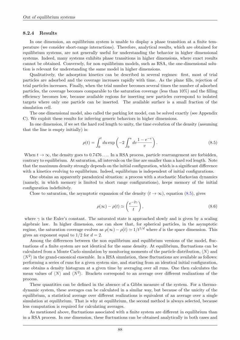
Out of equilibrium systems
8.2.4 Results
In one dimension, an equilibrium system is unable to display a phase transition at a finite tem-perature (we consider short-range interactions). Therefore, analytical results, which are obtained forequilibrium systems, are not generally useful for understanding the behavior in higher dimensionalsystems. Indeed, many systems exhibits phase transitions in higher dimensions, where exact resultscannot be obtained. Conversely, for non equilibrium models, such as RSA, the one-dimensional solu-tion is relevant for understanding the same model in higher dimensions.
Qualitatively, the adsorption kinetics can be described in several regimes: first, most of trialparticles are adsorbed and the coverage increases rapidly with time. As the plane fills, rejection oftrial particles increases. Finally, when the trial number becomes several times the number of adsorbedparticles, the coverage becomes comparable to the saturation coverage (less than 10%) and the fillingefficiency becomes low, because available regions for inserting new particles correspond to isolatedtargets where only one particle can be inserted. The available surface is a small fraction of thesimulation cell.
The one dimensional model, also called the parking lot model, can be solved exactly (see AppendixC). We exploit these results for inferring generic behaviors in higher dimensions.
In one dimension, if we set the hard rod length to unity, the time evolution of the density (assumingthat the line is empty initially) is:
ρ(t) =
∫ t
0du exp
(−2
∫ u
0dv
1− e−v
v
). (8.5)
When t→∞, the density goes to 0.7476 . . .. In a RSA process, particle rearrangement are forbidden,contrary to equilibrium. At saturation, all intervals on the line are smaller than a hard rod length. Notethat the maximum density strongly depends on the initial configuration, which is a significant differencewith a kinetics evolving to equilibrium. Indeed, equilibrium is independent of initial configurations.
One obtains an apparently paradoxical situation: a process with a stochastic Markovian dynamics(namely, in which memory is limited to short range configurations), keeps memory of the initialconfiguration indefinitely.
Close to saturation, the asymptotic expansion of the density (t→∞), equation (8.5), gives
ρ(∞)− ρ(t) '(e−2γ
t
), (8.6)
where γ is the Euler’s constant. The saturated state is approached slowly and is given by a scalingalgebraic law. In higher dimension, one can show that, for spherical particles, in the asymptoticregime, the saturation coverage evolves as ρ(∞)− ρ(t) ' 1/t1/d where d is the space dimension. Thisgives an exponent equal to 1/2 for d = 2.
Among the differences between the non equilibrium and equilibrium versions of the model, fluc-tuations of a finite system are not identical for the same density. At equilibrium, fluctuations can becalculated from a Monte Carlo simulation by monitoring moments of the particle distribution, 〈N〉 and〈N2〉 in the grand-canonical ensemble. In a RSA simulation, these fluctuations are available as follows:performing a series of runs for a given system size, and starting from an identical initial configuration,one obtains a density histogram at a given time by averaging over all runs. One then calculates themean values of 〈N〉 and 〈N2〉. Brackets correspond to an average over different realizations of theprocess.
These quantities can be defined in the absence of a Gibbs measure of the system. For a thermo-dynamic system, these averages can be calculated in a similar way, but because of the unicity of theequilibrium, a statistical average over different realizations is equivalent of an average over a singlesimulation at equilibrium. That is why at equilibrium, the second method is always selected, becauseless computation is required for calculating averages.
As mentioned above, fluctuations associated with a finite system are different in equilibrium thanin a RSA process. In one dimension, these fluctuations can be obtained analytically in both cases and
88

8.3 Avalanche model
their are less pronounced in a RSA process. This behavior is similar in higher dimensions, where onlynumerical results can be obtained. The analysis of fluctuations of adsorbed configurations allows oneto distinguish equilibrium and irreversible kinetics.
As seen in Chapter 4, the correlation function g(r) can be defined from geometrical considerations(for hard particles) and not necessarily by using a Gibbs measure. Consequently, it is possible tocalculate in a RSA process, pair correlations. By using the statistical average defined above (forfluctuation computation), one obtains g(r) at a given time by using several realizations.
A significant result of the structure is that at saturation, the pair distribution diverges logarith-mically at contact:
g(r, ρ∞) ∼ ln
((r − 1)
σ
). (8.7)
This feature is specific to an RSA kinetics. At equilibrium, at the same density, the pair distributionfunction g(r) is always finite at contact, in particular at density corresponding to the saturation densityof the RSA process.
8.3 Avalanche model
8.3.1 Introduction
Twenty five years ago, Bak, Tang et Wiesenfeld[2] introduced a model in order to explain thedynamic behavior of avalanches in a sand heap. Indeed, if one drops continuously sand particles abovea surface at a given point, one observes the formation of a heap, whose shape looks like a cone with anangle which can not exceed a critical value. Once reached this state, if sand particles are added again,one observes at different times avalanches of different sizes. This phenomenon seems independent ofthe microscopic nature of interactions between particles. Therefore, this simple model with non-linearrules is able to reproduce kinetics of avalanches.
8.3.2 Definition
For a square lattice in two dimensions (N ×N), one assumes that at each node, one has a integerz(i, j) associated with the site (i, j). This variable is considered as the local slope of the sand heap.The rules of the kinetics are the following:
1. At time t, one chooses randomly a site of the square lattice denoted i0, j0. One increments thesite value by one
z(i0, j0)→ z(i0, j0) + 1
t→ t+ 1.(8.8)
2. If z(i0, j0) > 4, the local slope becomes too high, and it triggers a particle spreading on nearestneighbor sites according the following rules:
z(i0, j0) → z(i0, j0)− 4
z(i0 ± 1, j0) → z(i0 ± 1, j0) + 1
z(i0, j0 ± 1) → z(i0, j0 ± 1) + 1
t→ t+ 1.
(8.9)
3. Particle spreading can increase the local slope on these sites, and if a local slope becomes largerthan the threshold value, this site also triggers a local avalanche (step 2)...
89

Out of equilibrium systems
For boundary sites, one considers that particles can be lost and the kinetic rules are the fol-lowing
z(0, 0) → z(0, 0)− 4
z(1, 0) → z(1, 0) + 1
z(0, 1) → z(0, 1) + 1
t→ t+ 1.
(8.10)
In this case, two particles leave the simulation box.
For i between 1 and N − 2 z(0, i) → z(0, i)− 4
z(1, i) → z(1, i) + 1
z(0, i± 1) → z(0, i± 1) + 1
t→ t+ 1.
(8.11)
In this case, only one particle leaves the simulation box.
One can also modify the kinetic rules on the box boundaries, by modifying the thresholds ofthe boundary sites. For instance, for a site of the corner of the box, the threshold is then equalto 2 and one has
z(0, 0) → z(0, 0)− 2
z(1, 0) → z(1, 0) + 1
z(0, 1) → z(0, 1) + 1
t→ t+ 1.
(8.12)
For i between 1 and N − 2, the threshold is equal to 3z(0, i) → z(0, i)− 3
z(1, i) → z(1, i) + 1
z(0, i± 1) → z(0, i± 1) + 1
t→ t+ 1.
(8.13)
In a similar way, one can write kinetic rules for all boundary sites.
A cycle continues until no site variable is less than the threshold value. 1. When the cycle isfinished, one restarts the step 1.
This algorithm can easily be adapted for different lattices and space dimensions.
The quantities, which can be monitored in simulation are the following: particles involved in anavalanche, namely number of sites which were in a critical state before adding anew particle (step 1).On can consider the particle distribution of lost particles (on the boundaries of the simulation box)along the process. Lastly, the frequency and the size distributions of avalanches are also interestingquantities.
8.3.3 Results
The significant results of this toy model are the following:
— Distribution of particle number in avalanches has a scaling law
N(s) ∼ s−τ (8.14)
where τ ' 1.03 in two dimensions.
1. Because sites which are critical at a given t are not nearest neighbor sites, the order in which update is done doesnot change the final state of the cycle. In others words, the model is Abelian.
90

8.4 Inelastic hard sphere model
— Avalanches occur randomly and their frequencies depend on the size s with a scaling law
D(s) ∼ s−2. (8.15)
— If the time associated with the elementary steps in an avalanche is T , the numnber of avalanchesof T time steps is given by
N ∼ T−1. (8.16)
It is interesting to compare the main features of this model with the basic features of systems atequilibrium.
A specific feature of this model is that the system evolves spontaneously towards a critical state,because spatially (avalanche distribution) and temporally, it is the analog of a critical point of anequilibrium system. However, in a equilibrium system, a critical point is associated with a fine tuningof a intensive parameter, like the temperature. In the avalanche model, there is no control parameters(temperature, pressure,...) and the system evolves to a critical state. Indeed, the value of the particleflux is an irrelevant quantity (but must be nonzero), and the avalanche distribution is unchanged. Theauthors who introduced this model, referred to this state as Self-Organized Criticality (SOC)[30, 2]).
The characteristics of this model have fascinated a wide community of scientists, beyond statisticalphysicists. Many variants of the original model have been studied, and the behavior observed in thetoy model is robust and can be recovered in many physical situations. For instance, in seismology,earthquakes are present in regions where the constraints are accumulated. A universal behavior ofearthquakes is the following: although it is hard to predict the date when an event can occur, aswell the intensity, one observes that the intensity distribution obeys a scaling law, with an exponentα ' 2. The same quantity monitored in the avalanche model gives an exponent α = 1, which givesa qualitative description of the earthquake statistics. More refined models are necessary for a moreprecise agreement.
Forest fires are a second example for which the analogy with the avalanche model is interesting. Ina first period, the forest grows on the surface, but it can be destroyed partially or totally by a forestfire. In the models used for the description of this phenomenon, there are two time scales: the firstone is associated with the random drop of trees on a given lattice; the second one is the inverse of thefrequency of fire triggering at a random position. 2. Fire propagates if the nearest neighbor sites areoccupied by a tree. Area distribution of burned forests is experimentally described by a scaling lawwith α ' 1.3− 1.4, close to the prediction of the SOC model.
We finish this section by returning to the initial objectives of the model. Are the observedavalanches in sand heaps described by this kind of model? The answer is rather negative. In most ex-periments, the frequency of the avalanche distribution is not uniformly distributed but rather sharplypronounced around a a given frequency. The size distribution is not given by a scaling law. It ispossible that the inertial and cohesive effects be neglected in the simple model could be responsiblefor the absence of a pure critical behavior. The system which seems to behave like a SOC model, isan assembly of rice grains, where scaling laws are observed 3
8.4 Inelastic hard sphere model
8.4.1 Introduction
Granular matter (powders, sands, ...) is characterized by the following properties: particle size ismuch larger than the atomic scales (at least several hundreds micrometers); the range of interactionbetween particles is less than the typical particle size; when particles collide, a fraction of the kineticenergy is lost and transformed in local heating; the particle mass being much larger than atoms, the
2. Obviously, experimental realization is prohibitive.3. you can try to test the truth fo these results in your kitchen, but I cannot held responsible for any damages.
91

Out of equilibrium systems
thermal energy is negligible compared to gravitational energy and power supply (generally, providedby vibrations).
In the absence of a continuous power supply, a granular system looses rapidly this initial kineticenergy, which is transformed in heat. At a macroscopic level (which corresponds to the observation),the system appears as dissipative. Taking account of the time scale separation, one can considersthat the collision time is negligible compared to the characteristic time of free steaming. Because theinteractions are short ranged and particle shape is not modified with collisions (we consider “gentle”collisions), one can assume that the interaction potential is hard core potential.
The total momentum of the two particles involved in a collision is conserved:
v1 + v2 = v′1 + v′2. (8.17)
During the collision, the relative velocity of the point of impact is changed as follows: Assuming thatthe tangential component of the velocity is conserved (which corresponds to a tangential coefficient ofrestitution equal to 1) one has the following relation
(v′1 − v′2).n = −e(v1 − v2).n (8.18)
where e is the normal coefficient of restitution and n is a normal unit vector, whose direction isgiven by the straight line joining the two centers of colliding particles. The value of this coefficient isbetween 0 and 1; the latter corresponding to a system of elastic hard spheres .
8.4.2 Definition
The inelastic hard sphere model is defined as a system interacting by a hard core potential andloosing kinetic energy in collisions. Combining the conservation of the total impulse and the collisionrules, one obtains the postcollisional velocities:
v′i,j = vi,j ±1 + e
2[(vj − vi).n]n (8.19)
with
n =r1 − r2
|r1 − r2|. (8.20)
This model is suitable for Molecular Dynamic simulations. We saw in Chapter 3 the algorithmof Molecular Dynamics of (elastic) hard spheres; it is easy to adapt this algorithm for inelastic hardspheres. The difference between the two systems, concerns the equations for updating velocities, whichimplies that the inelastic hard spheres looses continuously a fraction of its kinetic energy.
8.4.3 Results
The dissipative nature of collisions has some consequences: when one studies a granular systemin a steady state, it is necessary to inject energy in the system. Moreover, when the density of thesystem is moderate or large, particles rapidly form aggregates. This last phenomenon always existseven at low density where even one starts with a uniform distribution of particles, the system evolvestowards a state composed of clusters. The local density of clusters is then much larger than the initialuniform density and there are large regions of low density.
When the particle density increases sufficiently, the phenomenon od inelastic collapse will stop thesimulation. Since the system loses kinetic energy, one has configurations in which three particles ormore can trap one particle. Time evolution of the simulation is then dominated by a sequence ofcollisions between the central particle and its neighbors with a collision time which rapidly decreasesto zero. Asymptotically, one obtains a glued set of particles. 4.
This effect, which occurs in a simulation for a small group of particles, can be understood byconsidering the simple phenomenon of a single particle bouncing on a plane under the influence of
4. Particles are not strictly glued but the simulation is practically stopped, because this corresponds to an infinitesequence of collisions which occurs in a finite time.
92

8.4 Inelastic hard sphere model
gravity. Let h denotes the height at which the ball is dropped. At the first collision between theparticle and the plane, the elapsed time is t1 =
√2h/g and the precollisional velocity is
√2gh. After
the first collision, the velocity becomes e√
2gh. When the second collision occures, the elapsed timeis,
t2 = t1 + 2et1 (8.21)
and for the n collision, one has
tn = t1
(1 + 2
n−1∑i=1
ei
). (8.22)
Therefore, for an infinite number of collisions, one has
t∞ =t1
(1 +
2e
1− e
)(8.23)
=t11 + e
1− e(8.24)
A finite time of duration is elapsed until the bead comes to rest on the plan, whereas an infinitenumber of collisions was performed.
Because computation of a collision is proportional to the number of collisions, when an inelasticcollapse occurs, the simulation does not evolve longer in time. For real systems, when the relativevelocity at the point of impact becomes very small, collision does not remain inelastic, and the coeffi-cient of restitution goes to one when the relative velocity goes to zero. Indeed, the assumption of thecoefficient of restitution is constant is valid for collision velocities comparable to the thermal veloci-ties. For very large velocities, plastic deformation of hard particles are significant and the coefficientof restitution decreases for large velocities. Conversely, when velocities go to zero, the coeffficient ofrestitution goes to 1, and particle collisions become quasi elastic.
Even though, one expects the total kinetic energy to decrease to zero with time (unless there is apower supply that compensates the dissipation due to collisions), simulation of inelastic hard spherescannot reach this state, because simulation is stopped by the phenomenon of inelastic collapse.
If one wants to have a realistic model, it is necessary to consider how to supply power for a systemstudied in a steady state. In three dimensions, there is generally a vibrating wall whose collisions withparticles supply energy to the system. In a steady state, collisions between particles, which dissipateenergy, are compensated by collisions between particles and the vibrating wall.
In summary, the inelastic hard sphere model is a basic model for modeling granular gases.
8.4.4 Some properties
In the absence of a power supply, the system decreases continuously the temperature, there is ascaling regime before cluster formation in which the system remains homogeneous and whose velocitydistribution is expressed as a scaling function. To understand this regime, one considers the loss ofkinetic energy resulting from a collision between two particles. By using equation (8.19), one obtains
∆E = −1− α2
4m((vj − vi).n)2 (8.25)
One obviously notes that if α = 1 (elastic spheres), the kinetic energy is conserved, as seen in chapter3.Conversely, the energy loss is maximum when the coefficient of restitution is equal to 0.
With the assumption of a homogeneous system, the mean collision frequency is proportional tol/∆v. The mean energy loss is given by ∆E = −ε(∆v)2 where ε = 1−α2, which gives the evolution
dT
dt= −εT 3/2 (8.26)
and then the cooling law
T (t) ' 1
(1 +Aεt)2(8.27)
93

Out of equilibrium systems
This is known as the Haff’s law (1983).
When the granular system has an external source of energy, it reaches a steady state where theproperties are different from equilibrium. In particular, the velocity distribution is never Gaussian.This implies that the granular temperature defined as the mean square velocity is different from ofthe temperature associated with the width of the velocity distribution. One can show that the tailsof the velocity distribution do not decay as a Gaussian generally, and that the shape is closely relatedto the details of the power supply.
Among the specific properties, note that in a mixture de two species of granular particles (forinstance, different sizes of particles), the granular temperatures of each specie are differnt: there is noequipartition contrary to equilibrium.
8.5 Exclusion models
8.5.1 Introduction
Whereas the Gibbs-Botzmann distribution is central to equilibrium statistical mechanics owns,there is no general method for obtaining the configuration distribution for a steady state of a system.Exclusion models are toy models that they have beeen extensively studied by theory and simulations.These models can be used for describing vehicular traffic, in particular, for phenomena as traffic jamsas well as fluctuation currents which spontaneously appear when the car density increases.
Many variants of the original model exist and we restrict our attention to basic examples in orderto exhibit the most significant properties. In theoretical treatments, the one dimensional version ofthese models are most studied.
Consider a one dimensional lattice of N sites where n particles are placed. Each particle has ahopping probability p on the right si the nearest site is empty and a hopping probability 1− p on theleft if the nearest site is empty.
For non equilibrium systems, the details of the stochastic dynamics can be relevant for propertiesof the system. For these models, one can choose among at least three different methods for thedynamics.
— Parallel update: at the same time, all rules are applied to particles. This dynamics is sometimescalled synchronous update. This kind of dynamics leads to significant particle correlations. Thecorresponding master equation is a finite difference equation in time. 5
— Asynchronous update. This corresponds to the most used algorithm by choosing randomly anduniformly a particle at time t and to apply the update rules of the model. The correspondingmaster equation is a differential equation.
— When the update is sequential and ordered, one considers successive sites of the lattice. Order-ing can be chosen from the left to the right or conversely. The corresponding equation is alsofinite difference equation in time.
8.5.2 Random walk on a ring
Stationary state and detailed balance
When the systems has periodic boundary conditions, the walker which reached the site N has aprobability p of hopping on the site 1. It is easy to find out that such a system has a stationary statewhere the the probability of being on a site is independent of the site and is equal to Pst(i) = 1/N .
5. For the ASEP model, for avoiding overlap between particle hopping from the left or from the right at the sametime, the algorithm considers alternatively a parallel update on a sub-lattice, which prevents the overlap configurationof two particles coming from the left and from the right at the same time. Therefore, one performs the parallel updateon the first sub-lattice of even sites and a parallel update on the sublattice of odd sites.
94
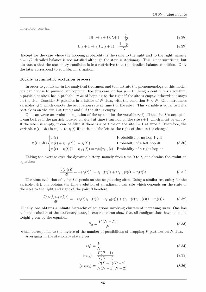
8.5 Exclusion models
Therefore, one has
Π(i→ i+ 1)Pst(i) =p
N(8.28)
Π(i+ 1→ i)Pst(i+ 1) =1− pN
(8.29)
Except for the case where the hopping probability is the same to the right and to the right, namelyp = 1/2, detailed balance is not satisfied although the state is stationary. This is not surprising, butillustrates that the stationary condition is less restrictive than the detailed balance condition. Onlythe later correspond to equilibrium situation.
Totally asymmetric exclusion process
In order to go further in the analytical treatment and to illustrate the phenomenology of this model,one can choose to prevent left hopping. For this case, on has p = 1: Using a continuous algorithm,a particle at site i has a probability dt of hopping to the right if the site is empty, otherwise it stayson the site. Consider P particles in a lattice of N sites, with the condition P < N . One introducesvariables τi(t) which denote the occupation rate at time t of the site i. This variable is equal to 1 if aparticle is on the site i at time t and 0 if the site is empty.
One can write an evolution equation of the system for the variable τi(t). If the site i is occupied,it can be free if the particle located on site i at time t can hop on the site i+ 1, which must be empty.If the site i is empty, it can be filled if there is a particle on the site i − 1 at time t. Therefore, thevariable τi(t+ dt) is equal to τi(t) if no site on the left or the right of the site i is changed
τi(t+ dt)
τi(t) Probability of no hop 1-2dt
τi(t) + τi−1(t)(1− τi(t)) Probabilty of a left hop dt
τi(t)− τi(t)(1− τi+1(t)) = τi(t)τi+1(t) Probabilty of a right hop dt
(8.30)
Taking the average over the dynamic history, namely from time 0 to t, one obtains the evolutionequation:
d〈τi(t)〉dt
= −〈τi(t)(1− τi+1(t))〉+ 〈τi−1(t)(1− τi(t))〉 (8.31)
The time evolution of a site i depends on the neighboring sites. Using a similar reasoning for thevariable τi(t), one obtains the time evolution of an adjacent pair site which depends on the state ofthe sites to the right and right of the pair. Therefore,
d(〈τi(t)τi+1(t)〉)dt
= −〈τi(t)τi+1(t)(1− τi+2(t)〉) + 〈τi−1(t)τi+1(t)(1− τi(t))〉 (8.32)
Finally, one obtains a infinite hierarchy of equations involving clusters of increasing sizes. One hasa simple solution of the stationary state, because one can show that all configurations have an equalweight given by the equation
Pst =P !(N − P )!
N !(8.33)
which corresponds to the inverse of the number of possibilities of dropping P particles on N sites.Averaging in the stationary state gives
〈τi〉 =P
N(8.34)
〈τiτj〉 =P (P − 1)
N(N − 1)(8.35)
〈τiτjτk〉 =P (P − 1)(P − 2)
N(N − 1)(N − 2)(8.36)
95

Out of equilibrium systems
0 0.5 1α
0
0.5
1
β
CPLDP
HDP
Figure 8.2 – Phase diagram of ASEP model. The dashed line is a first-order line transition and thetwo full curves correspond to continuous transition lines.
8.5.3 Model with open boundaries
By using open boundaries, the system can exchange particles with“reservoirs”. If the site 1 is emptyat time t, there is a probability (or a probability density for a continuous dynamics) α of injecting aparticle at site 1, and if the site is occupied, there is a probability γ of removing the particle from theleft site of the lattice. Similarly, if the site N is occupied, there is a probability β of removing theparticle from the right side of the lattice and if the site N is empty, there is a probability δ of insertinga particle on site N .[6, 21]
On can write equations of time evolution in general, but analytical solutions cannot be obtained.For the sake of simplicity, we restrict ourselves to the totally asymmetric case. The evolution equationsobtained for the system with periodic boundary conditions are the same for sites 2 to N − 1, and forthe sites 1 and N they are modified as follows: the site 1, if empty, can accept a particle from thereservoir with a probability α and, if occupied, lose its particle, either because the particle hops intothe reservoir with the probability γ, or it hops on the right site. One then obtains
d〈τ1(t)〉dt
= α(1− 〈τ1(t)〉)− γ〈τ1(t)〉 − 〈τ1(t)(1− τ2(t))〉 (8.37)
In a similar manner for the site N , one has
d〈τN (t)〉dt
= 〈τN−1(t)(1− τN (t))〉+ δ〈(1− τN (t))〉 − β〈τN (t)〉 (8.38)
It is possible to derive a solution in the stationary state. We only summarize basic features of themodel by drawing the phase diagram, in the case where δ = γ = 0, see figure 8.2.
The LDP (low density phase) region corresponds to a stationary density (in bulk) equal to α ifα < 1/2 and α < β. The HDP (high density phase) region corresponds to a stationary density 1− βand occurs for values of β < 0.5 and α > β. The last region of the phase diagram is called maximalcurrent phase and corresponds to values of α and β strictly larger than 1/2. The dashed line denotesthe boundary between the LCP et HDP phase and corresponds to a first-order transition line. Indeed,in the thermodynamic limit, crossing the transition line leads to a density discontinuity
∆ρ = ρHCP − ρLCP= 1− β − α (8.39)
= 1− 2α (8.40)
96

8.6 Kinetically constrained models
which is nonzero for α < 0.5. For a simulation where one has a finite system, one obtains a rapidlyvariation with a increasing slope when the system size increases.
8.6 Kinetically constrained models
8.6.1 Introduction
When a liquid is supercooled, the relaxation time increases by fifteen orders of magnitude andthe liquid becomes a glass, which corresponds to a non equilibrium state. The glass transition isassociated with the phase change, but contrary to other transitions (liquid-gas, liquid-solid,...), nodiverging length is unambiguously identified, no significant structural change can be monitored. Inorder to gather data associated with many glassformers, it is useful to show the fast increase ofrelaxation times (or the viscosity) as a function of the inverse of the temperature normalized for eachglassformer with its temperature of glass transition. 6
Figure 8.3 shows the Angell diagram for different systems. A straight line in this diagram corre-sponds to a strong glass whereas a curved line is characteristic of a fragile glass. The fragility increaseswith curvature ; in this diagram, the most fragile glass is the orthoterphenyl.
For strong glasses, the temperature dependence is
τ = τ0 exp(E/T ) (8.41)
where E is an activation energy which is independent of the temperature.For fragile glasses, several proposed fits are associated with the absence of a specific temperature
relevant to the phenomenon; A possible scenario is the existence of a temperature (below the glasstransition) and a putative transition not accessible to experiments . The Vogel-Fulscher-Thalmann(VFT) law provides accurate fits of the relaxation time versus temperature and is given by the relation
τ = τ0 exp(A/(T − T0)). (8.42)
The temperature T0 is often interpreted as a transition temperature, where the transition can bereached experimentally. An alternative interpretation consists of considering the ratio A/(T − T0) asan activation energy which increases rapidly when the system is cooled. Another suggestion consistentwith fragile behavior is given by the relation
τ = τ0 exp(B/T 2) (8.43)
This fit gives an accurate description of the relaxation time as a function of temperature for severalglassformers.
A second characteristic of supercooled liquids is the slow, non exponential decay of correlationfunctions. This behavior is usually fitted by a Kohraush-Williams-Watts law, which is expressed as
φ(t) = exp(−atb) (8.44)
where φ(t) is the correlation function of the measured quantity. Generally, b is a decreasing function ofthe temperature. b is an exponent starting from 1 at high temperature (region where correlation func-tions decasy exponentially) to 0.5 to 0.3 close the glass transition. One can also write the correlationfunction as
φ(t) = exp(−(t/τ)b) (8.45)
where τ = a−1/b. This is corresponds to a stretched exponential, The strechting is significant whenthe exponent is small.
There are three different procedures to determine the characteristic relaxation time of the correla-tion function,
6. This temperature is defined with an experimental protocol where the relaxation time reaches the value of 1000s.The temperature of glass transition depends on how fast the system is cooled.
97

Out of equilibrium systems
Figure 8.3 – Logarithm of the viscosity (or relaxation time) as a function of the inverse of the normalizedtemperature of the glass transition of each glassformer. Germanium oxide is considered a strong glasswhereas orthoterphenyl is the most fragile glass.
— Consider that the characteristic time is given by φ(τ) = 0.1φ(0). This method is used both insimulation and in experiments, Because the statistical fluctuations are generally smaller then0.1φ(0), τ can be obtained with a good accuracy. Conversely, if one chooses φ(τ) = 0.01φ(0)the signal to noise ratio is too low for obtaining the time relaxation.
— More rigorously, on can say that the characteristic relaxation time is given by the integral ofthe correlation function. τ =
∫∞0 dtφ(t). This method is interesting when the decay of the
correlation function is fast.— On can determine the relaxation time from the fitting law, Eq.(8.45), but one must find at the
same time the exponent of the stretched exponential.
When the correlation function is described by a simple exponential, the three methods providesimilar relaxation times. In general, there is no simple relation between the relaxation times cal-culated by the three different methods. However, when the decay of the correlation function has ashape of type KWW and the exponent b is not too small (which corresponds to many experiments ofglassformers), the relation between the three times is simple. Therefore the first method is generallyused in simulation.
A final characteristic of glassformers is the existence of heterogeneous relaxation: In other words,the supercooled liquid split into regions with different characteristic relaxation times. The global relax-ation would be the superimposition of “individual” relaxations. An interpretation of this phenomenonleads to a KWW law; indeed, if each domain relaxes exponentially with a typical relaxation frequencyν, the total relaxation is given by
φ(t) =
∫dνexp(−tν)D(ν) (8.46)
Mathematically, this corresponds to the Laplace transform of the frequency density of different do-mains.
98

8.6 Kinetically constrained models
8.6.2 Facilitated spin models
Introduction
Because glassy behavior is common to many different systems, including polymers and granularmatter, it seems reasonable to consider coarse-grained approaches. Kinetically constrained modelsare based on this idea. By considering that the heterogeneous dynamics is at the origin of the slowrelaxation observed in glassy systems, many lattice models with discrete variables have been proposed.The virtue of these models, is that, starting with a trivial thermodynamics, restriction of the standardMetropolis rules can lead to non trivial dynamics and can reproduce a significant part of the observedphenomena[24]. Because the origin of the glass transition is still being debated, we do not discussthe relevance of these models, but we focus on the drastic changes of the dynamics caused by theintroduction of some local rules. In the next chapter, we wiil consider an second example (adsorption-desorption model) where the absence of diffusion compared to a standard dynamics leads to a slowand non trivil relaxation.
Friedrickson-Andersen model
Twenty five years ago, Friedrickson and Andersen introduced the following model: Consider alattice (in one-dimension, for the sake of simplicity), On each site, one has a boolean variable, denotedby ni. The Hamiltonian reads
H =N∑i=1
ni (8.47)
At a given temperature T (the inverse temperature is β = 1/kBT ), one has the density of (“mobile”)n in the state 1, which is given by
n =1
1 + exp(β)(8.48)
Particles which are mobile are in the state 1 whereas particles in the state 0 are sluggish. Thismodel mimics a heterogeneous dynamics. At low temperature, the density of mobile particles is smalln ∼ exp(−β). Using Metropolis rules, four elementary configuration changes have to be considered.The rule corresponding to a state change does not depend on the neighborhood, but one has
...000...↔ ...010... (8.49)
...100...↔ ...110... (8.50)
...001...↔ ...011... (8.51)
...101...↔ ...111... (8.52)
The Friedrickson-Andersen model removes the configuration change of the first of the four situa-tions, which corresponds to preventing the creation or destruction of a mobile particle surrounded byimmobile particles. By restricting the dynamics, one can explore all configurations of the phase spaceexcept one configuration where all particles are immobile and cannot be reached.
In this case, one can show that the relaxation time evolves in one dimension as
τ = exp(3β) (8.53)
which corresponds to a strong glass behavior with a activated process dynamics.
East Model
Refs.[[24, 20, 20]] This model is inspired by the preceding model: the Hamiltonian is the same, butthe dynamics is more restrictive with a left-right symmetry breaking. Indeed, the dynamic rules arethe same as the preceding model, except the rule, Eq.(8.51), and mobile particles are only created if
99

Out of equilibrium systems
a mobile particleexists on the right. One can easily check that all configurations are available (exceptthe configuration of immobile particles) but with the additional rule the characteristic time becomes
τ = exp(1/(T 2 ln(2)) (8.54)
Because the relaxation time increases more rapidly than observed in a Arrhenius law, this modelhas a dynamics alike to a fragile glass whereasd the FA model behaves as a strong glass. With thesesimple rules, it is possible to perform very accurate numerical simulations at equilibrium and also innon equlibrium situations, which allows one to compare to theoretical approaches.
8.7 Conclusion
These different models illustrate the diversity of behaviors and therefore the richness of phenomenain out-of-equilibrium situations. Because no general theory is available for non equilibrium systems,numerical simulation is a powerful tool for investigating systems and also for testing theoretical ap-proaches that have been developed on simple models.
100

9Slow kinetics, aging.
9.1 Introduction
In the previous chapter, we have shown that the diversity of behaviors by considering differentsimple models whose kinetics do not reach equilibrium. In many situations, even if the relaxation timeis finite, the observation time may be significantly smaller than the relaxation time and the systemremains out-of-equilibrium with a very slow evolution. In this case, quantities of interest (in simulationor in an experiment) depends of the initial state of the system. This means that, if two experimentsin the same system are performed sequentially (with a very large waiting time), quantities of interestare not identical. For a long time, this was a significant barrier for understanding the properties of asystem.
Thanks to many experiments (spin glasses, polymer aging, granular matter,...), theoretical worksin domain growth (numerical simulation and exact results) and spin dynamics of spin models (in thepresence of quenched disorder), some general features of non-equilibrium systems have emerged.
The statistical physics of out-of-equilibrium systems rapidly evolving, numerical simulation is apowerful tool for investigating the dynamics and providing detailed information about the propertiesof the systems.
9.2 Formalism
9.2.1 Two-time correlation and response functions.
When the relaxation time is much larger than the observation time, the system cannot be consideredat equilibrium at any time.
Therefore, one must consider not only the elapsed time τ of the experiment (like at equilibrium),but also the waiting time tw, corresponding to the duration between the initial time when the systemwas prepared and the time when the experiment begins. Assuming that the system is at equilibriumat high temperature T at time t = 0, one performs a rapid quench to a lower temperature T1. Lettw denote the elapsed time between the quench and the beginning of experiment. For a quantity A,function of microscopic variables (magnetization for a spin model, positions and velocities of particlesin a liquid
”...), one defines the two-time correlation function CA(t, tw) as
CA(t, tw) = 〈A(t)A(tw)〉 − 〈A(t)〉〈A(tw)〉. (9.1)
The angular bracket denotes an average over a large number of realizations where the system wasinitially at equilibrium before the quench. 1.
1. At high temperature, the relaxation time is generally short and the system reaches equilibrium rapidly. After arapid quench at time t = 0, the system evolves naturally and at tw, the experiment starts and the time correlationfunction is then monitored.
101

Slow kinetics, aging.
Similarly, one defines a response function for the variable A. If h is the external field conjugate toA (δE = −hA), the two-time response function is given by the functional derivative of the variable Awith respect to the field h:
RA(t, tw) =
(δ〈A(t)〉δh(tw)
)h=0
. (9.2)
In simulation (or in experiement), it is easier to calculate the integrated response function which isdefined as
χA(t, tw) =
∫ t
tw
dt′RA(t, t′) (9.3)
In other words, the response function can be expressed as
〈A(t)〉 =
∫ t
tw
dsRA(t, s)h(s) +O(h2) (9.4)
Since causality is satisfied, the response function obeys
RA(t, tw) = 0, for t < tw. (9.5)
9.2.2 Aging and scaling laws
At least, two time-scales characterize the dynamics of a system: a typical time scale associatedwith a local rearrangement of the system (mean time for a spin flip in a lattice model), that wecalled microscopic time t0, and a relaxation time teq associated with the typical time scale for reachingequilibrium. When the waiting time tw and the experiment time τ are between the following timeintervals
t0 << tw << teq (9.6)
t0 << tw + τ << teq, (9.7)
the system is not equilibrated and is unable to reach equilibrium on a time scale associated withexperiment.
In many experiments, as well as in solutions of exact models (corresponding to a mean-field ap-proximation) the correlation function can be expressed as the sum of two contributions:
CA(t, tw) = CST (t− tw) + CAG
(ξ(tw)
ξ(t)
)(9.8)
where ξ(tw) is a function depending on the system. This means that, for a short duration of time, thesystem behaves as if it were at equilibrium; this regime is described by the function CST (τ = t− tw),and is independent of the waiting time tw, as in a system at equilibrium.
For a domain growth of a ferromagnetic system, when one quenches the system at a temperaturelower than the critical temperature, the first term of equation (9.8) corresponds to the spin relaxationwithin a domain, whereas the second term depends on the waiting time and describes the relaxationof domain walls (where ξ(t) is the typical size of domains at time t).
The expression of “aging” is justified by the fact that, when one waits a longer time for measuringa quantity, the system needs more time to lose memory of the initial configuration.
The function ξ(tw) is not known in general, which means that it is necessary to propose trial
functions and to check if the correlation functions CAG
(ξ(tw)ξ(t)
)collapse in a master curve.
102

9.3 Adsorption-desorption model
9.2.3 Interrupted aging
When the second inequality of equation (9.7) is not satisfied, namely the time t becomes muchlarger than the equilibrium time teq, whereas tw is much smaller than teq, the system has an interruptedaging.
At times larger than the microscopic time, the system relaxes as an out-of-equilibrium system, i.e.with a non stationary part of the correlation function. At long times, the system reaches equilibrium,and the correlation function becomes translationally invariant in time and the fluctuation-dissipationtheorem holds again.
9.2.4 “Violation” of the fluctuation-dissipation theorem
For an equilibrium system, the response and correlation functions are translationally invariant intime RA(t, tw) = RA(τ = t − tw) et CA(t, tw) = CA(τ), and related by the fluctuation-dissipationtheorem (see Appendix A).
RA(τ) =
−βdCA(τ)
dττ ≥ 0
0 τ < 0(9.9)
This relation between the response function and the correlation function is valid only if the systemevolves towards equilibrium. 2. One often writes that for out-of-equilibrium systems there is violationof fluctutation-dissipation theorem, but the appropriate wording is that the FD theorem does not hold.Indeed, for out-of-equilibrium systems, the FD theorem is not violated since the basic assumptions ofthe proof are not satisfied.
Using analytical results obtained in solvable models and numerical simulation, one formally definesa relation between the response function and the assocaited correlation function,
RA(t, tw) = −βX(t, tw)∂CA(t, tw)
∂tw(9.10)
where X(t, tw) is then defined by this above equation: This function is a priori unknown.
For an equilibrium system, one has
X(t, tw) = 1. (9.11)
At short time, the correlation and response functions decay as stationary functions irrespective of thewaiting time; one then has
X(t, tw) = 1 τ = t− tw << tw. (9.12)
Beyond this regime, the system ages and the function Xo is different from 1.
In mean-field models, the fluctuation-dissipation ratio only depends on the correlation functionX(t, tw) = X(C(t, tw)) at long time. In this case, one can assume that the aging system is characterizedby an effective temperature
Teff (t, tw) =T
X(t, tw)(9.13)
9.3 Adsorption-desorption model
9.3.1 Introduction
We now illustrate the concepts introduced above by using the adsorption-desorption model. Thismodel has several advantages: it is an extension of the Parking model discussed in previous chapters; atlong time (which can be larger than the simulation time) the system reaches equilibrium. Consequently,by tuning one control parameter (basically the chemical potential which sets the equilibrium constant
2. The cornerstone of the proof is the knowledge of the equilibrium probability distribution.
103

Slow kinetics, aging.
between the adsorption and desorption rates), one has a model where one can observe equilibriumproperties to out-of-equilibrium properties.
The dynamics of this model is similar to a Monte Carlo simulation in a grand-canonical ensemble,except that the particles do not move on the line. Even through, at long time, the system evolvestowards equilibrium, the system relaxes extremely slowly (if the equilibrium density is high), and onecan observe the system aging.
Lastly, the adsorption-desortion model can be used as a phenomelogical approach for interpretingthe granular compaction.
9.3.2 Definition
Hard rods are dropped onto a line, with a constant rate k+. If the trial particle does not overlapother previously adsorbed particle, this particle is accepted, otherwise it is rejected and a new trialis performed. Moreover, particles are desorbed randomly and uniformly with a constant rate k−.For k− = 0, this model corresponds to the parking model for which the jamming limit is equal toρ∞ ' 0.7476 . . . . (if the line was empty initially). When k− 6= 0, but very small, the system evolvesvery slowly towards equilibrium.
Because the properties of the system only depend on the ratio K = k+/k−, and by using a changeof variable of unit of time, the time evolution of the system is expressed as
dρ
dt= Φ(t)− ρ
K, (9.14)
where Φ(t) is the probability of inserting a particle at time t.At equilibrium, one has
Φ(ρeq) =ρeqK
(9.15)
The insertion probability is then given by
Φ(ρ) = (1− ρ) exp
(−ρ
1− ρ
). (9.16)
By inserting equation (9.16) in equation (9.15), one obtains the equilibrium density
ρeq =Lw(K)
1 + Lw(K), (9.17)
where Lw(x), the Lambert-W function, is the solution of equation x = yey. In the limit of smallvalues of K, ρeq ∼ K/(1 +K), whereas for large values of K,
ρeq ∼ 1− 1/ ln(K). (9.18)
The equilibrium density ρeq goes to 1 when K → ∞. Let us note that there is a discontinuitybetween the limit K → ∞ and the case K = ∞, because the maximum densities are equal to 1 and0.7476 . . ., respectively.
9.3.3 Kinetics
Unlike the Parking model the kinetics of the adsorption-desorption model cannot be obtainedanalytically. It is however possible to analyze qualitatively the dynamics in different regimes. We onlyconsider the case where the desorption is weak 1/K << 1.
1. Until the density is smaller than the jamming limit of the Parking model, desorption can beneglected and for t ∼ 5, the density increases as for the Parking model, namely as 1/t.
2. When the interval of time between two adsorptions become comparable to the characteristictime of adsorption of a new particle, the density only increases if a desorbed particle freesenough room to accommodate two adsorptions. In this regime, one can show that the densityincreases as 1/ ln(t) (see figure 9.1).
104

9.3 Adsorption-desorption model
0 5 10 15
ln(t)
0.40
0.50
0.60
0.70
0.80
0.90
ρ(t)
1/ln(t)
1/t
e(-Γt)
Figure 9.1 – Density of the desorption-adsorption model as a function of time. Kinetics can be dividedin theee regimes at high density: the first one evolves as 1/t, the second one as 1/ ln(t) and the thirdone as an exponential exp(−Γt).
3. At long time, the system reaches equilibrium: desorption events become comparable to ad-sorption events and the density approaches equilibrium exponentially exp(−Γt), where Γ is theinverse of the relaxation time.
9.3.4 Equilibrium linear response
When the waiting time is much larger than the relaxation time at equilibrium, one must recoverthe fluctuation-dissipation theorem.
At equilibrium, the adsorption-desorption model corresponds to a hard rod model in a grand-canonical ensemble. with a chemical potential βµ = ln(K).
The integrated response function can be easily calculated
χeq = ρeq(1− ρeq)2. (9.19)
Similarly, one can calculate the equilibrium correlation function.
Ceq = ρeq(1− ρeq)2. (9.20)
Fluctuation-dissipation theorem gives
χ(τ) = C(0)− C(τ). (9.21)
For hard core particles, the temperature is an irrelevant parameter, which explains the slight modifi-cation of the the fluctuation-dissipation theorem. Figure 9.2 shows a parametric plot of the responsefunction χ(τ)/χeq versus C(τ)/Ceq. The diagonal corresponds to the value given by the fluctuation-dissipation theorem.
9.3.5 Hard rods age!
We are interested in non-equilibrium properties of the model in the kinetic regime 1/ ln(t), namelywhen the system does not reach equilibrium. The quantity of interest of this model is the (normalized)density correlation function, which is defined as
105

Slow kinetics, aging.
0 0.2 0.4 0.6 0.8
C(t,tw
)
0
0.2
0.4
0.6
0.8
1
χ(t,t
w)
Figure 9.2 – Normalized equilibrium integrated response function χ(τ) versus the normalized correla-tion function C(τ) for K = 300 (the waiting time is equal to tw = 3000 > teq ).
C(t, tw) = 〈ρ(t)ρ(tw)〉 − 〈ρ(t)〉〈ρ(tw)〉 (9.22)
where angular brackets denote an average over many independent runs.When τ and tw are large, but smaller than the equilibrium time τeq, aging is described by a scaling
function. For this model, on obtains a simple aging which corresponds to the following function
C(t, tw) = f(tw/t) (9.23)
9.3.6 Algorithm
The integrated response function is defined as
χ(t, tw) =δρ(t)
δ ln(K(tw)). (9.24)
In simulation, computation of the integrated response function requires, a priori, to perform a runin the presence of an external field. Unfortunately, choosing the intensity of the field is a challengingproblem: in order to obtain a linear response function, one has to choose a weak external field, butif this field is small, the response function which is defined as the ratio of the difference between twosimulations (the first one in the presence of an external field, the second one in the absence of a field)over the external field becomes very noisy when the field is small. One method used for minimizing theinfluence of non linear contributions consists of performing three simulations: one in the absence of anexternal field, two others in the presence of a positive and negative fields. Using a linear combinationof results, it is possible to cancel the quadratic term of the non linear response function, but cubicand higher odd orders terms are present.
The second method, proposed by L. Berthier[3], is more recent and has several adavantages: Onlyone run in the absence of an external field is necessary. The response function is calculated in thelimit of an infinitesimal field. The basic idea of the method consists of expressing the average in termsof probabilities of observing the system at time t
〈ρ(t)〉 =1
N
N∑k=1
ρ(t)Pk(tw → t) (9.25)
106

9.3 Adsorption-desorption model
where Pk(tw → t) is the probability that the kth trajectory (or simulation) goes from tw to t and kis index running over N independent trajectories.
Because the dynamics is Markovian, the probability Pk(tw → t) is expressed as the product oftransition probabilities of successive configurations of the system going from tw to t
Pk(tw → t) =t−1∏t′=tw
WCkt′→C
kt′+1
(9.26)
where WCkt′→C
kt′+1
is transition probability from the configuration Ckt′ of the kth trajectory at time t′
to the configuration of the kth trajectory Ckt′+1 at time t′ + 1. For a standard Monte Carlo dynamics,this transition probability is expressed as
WCkt→Ck
t+1= δCk
t+1C′tΠ(Ckt → C ′t) + δCt+1Ck
t(1−Π(Ckt → C ′t)) (9.27)
where Π(Ckt → C ′t) is the acceptance probability from the configuration Ckt at time t to the config-uration C ′t+dt at time t + dt. The second term of the right hand side of equation (9.27) accounts forthe fact that, if the configuration C ′t is rejected, the trajectory keeps the same configuration with thecomplementary probability.
The integrated susceptibility (integrated response function) is expressed as
χ(t, tw) =∂ρ(t)
∂h(tw)(9.28)
For the parking model, one has h = ln(K).By using the trajectory probabilities, one can write the susceptibility as
χ(t, tw) =1
N
N∑k=1
ρ(t)∂Pk(tw → t)
∂h(9.29)
If one adds an infinitesimal field, the transition probalities are modified and taking the logarithmof equation (9.25), one has
∂Pk(tw → t)
∂h= Pk(tw → t)
t−1∑t′=tw
∂ ln(WCkt′→C
kt′+1
)
∂h(9.30)
Therefore, the integrated response function is expressed as an average
χ(t, tw) = 〈ρ(t)H(tw → t)〉 (9.31)
where the brackets are the average over a trajectory in the absence of a field and with the functionHk(tw → t) whose expression is given by
Hk(tw → t) =∑t′
∂ ln(WCkt′→C
kt′+1
)
∂h(9.32)
On can easily compute the two-time correlation function by using the same trajectories (withoutfield). For estimating the fluctuation-dissipation ratio, one has the relation
∂χ(t, tw)
∂tw= −X(t, tw)
T
∂C(t, tw)
∂tw(9.33)
One can obtain the function X(t,tw)T by considering the local slope of the parametric plot. When
this function is a piecewise constant function, X(t, tw) is interpreted as an effective temperature. Itis important to stress that the parametric plot must be done at constant t and for different values ofthe waiting times tw, which is a consequence of equation (9.33). Indeed, the derivative is with respectof tw and not t. First studies were done incorrectly, and significant corrections are obtained with thecorrect method.
107

Slow kinetics, aging.
1 10 100t-t
w
0
0.001
0.002
0.003
0.004
1/ρ(
t)-1
/ρeq
(K=
500)
Figure 9.3 – Time evolution of the excess volume for the adsorption-desorption model 1/ρ(t) −1/ρeq(K = 500) as a function of t − tw. The upper curve corresponds to the case where K is de-creased from K = 5000 to K = 500 at tw = 240. The middle curve K is switched from K = 2000 toK = 500 at tw = 169, and the lower curve corresponds to the case where K decreases from 1000 to500 at tw = 139.
9.4 Kovacs effect
For systems with extremely large relaxation times, the response to a sequence of external fieldsleads to a behavior different to that observed at equilibrium. It seems that there is some universalbehavior of responses in out-of-equilibrium systems. The Kovacs effect is an example, that can beillustrated with the simple Parking model. Originally observed in polymers in sixties, this phenomenonis observed by performing the following sequence: A rapid quench at low temperature, where the systemremains a waiting time tw, and a rapid heating to an intermediate temperature. When the volumeof the polymer reaches the equilibrium volume in the heating phase, one then observes a volumeincrease and at long time the volume decreases in order to reach the equilibrium volume. This out-of-equilibrium phenomenon is universal and is present in the adsorption-desorption model. In figure 9.3,the maximum of the volume is more important when the quench is significant. This behavior was alsoobserved in fragile glassformers as well as in simulation.
9.5 Conclusion
The study of out-of-equilibrium phenomena is quite recent compared to equilibrium systems. Formore complex systems than described above and for which one has an hierarchy of time scales, it isnecessary to consider a sequence of aging, generalizing the simple scheme presented in this chapter:
CA(tw + τ, tw) = CST (τ) +∑i
CAG,i
(ξi(tw)
ξi(tw + τ)
)(9.34)
To obtain the typical time scales is obviously a difficult task. This could be what happens in manyglassy systems. Several methods have been proposed in the last ten years for numerical simulation andexperimental studies, in which the response of the system to an external field can provide significantinformation on the dynamic properties.
108

Bibliography
[1] B. J. Alder and T. E. Wainwright. Phase transition for a hard sphere system. J. Chem. Phys.,27(5):1208–1209, 1957.
[2] Per Bak, Chao Tang, and Kurt Wiesenfeld. Self-organized criticality: An explanation of the 1/fnoise. Phys. Rev. Lett., 59(4):381–384, Jul 1987.
[3] Ludovic Berthier. Efficient measurement of linear susceptibilities in molecular simulations: Ap-plication to aging supercooled liquids. Phys. Rev. Lett., 98(22):220601, 2007.
[4] K Binder. Applications of monte carlo methods to statistical physics. Reports on Progress inPhysics, 60(5):487–559, 1997.
[5] D. Chandler. Introduction to Modern Statistical Mechanics. Oxford University Press, New York,USA, 1987.
[6] B Derrida, M R Evans, V Hakim, and V Pasquier. Exact solution of a 1d asymmetric exclusionmodel using a matrix formulation. J. Phys. A: Math. Gen., 26(7):1493, 1993.
[7] C. Dress and W. Krauth. Cluster algorithm for hard spheres and related systems. Journal OfPhysics A-Mathematical And General, 28(23):L597–L601, December 1995.
[8] Alan M. Ferrenberg, D. P. Landau, and Robert H. Swendsen. Statistical errors in histogramreweighting. Phys. Rev. E, 51(5):5092–5100, 1995.
[9] Alan M. Ferrenberg and Robert H. Swendsen. New monte carlo technique for studying phasetransitions. Phys. Rev. Lett., 61:2635–2638, Dec 1988.
[10] Alan M. Ferrenberg and Robert H. Swendsen. Optimized monte carlo data analysis. Phys. Rev.Lett., 63(12):1195–1198, 1989.
[11] D. Frenkel and B. Smit. Understanding Molecular Simulation: from algorithms to applications.Academic Press, London, UK, 1996.
[12] Nigel Goldenfeld. Lectures on Phase Transitions and the Renormalization Group. Addison-Wesley,New-York, USA, 1992.
[13] J. P. Hansen and I. R. Mc Donald. Theory of simple liquids. Academic Press, London, UK, 1986.
[14] J. R. Heringa and H. W. J. Blote. Geometric cluster monte carlo simulation. Phys. Rev. E,57(5):4976–4978, May 1998.
[15] J. R. Heringa and H. W. J. Blote. Geometric symmetries and cluster simulations. Physica A,254(1-2):156–163, May 1998.
[16] Haye Hinrichsen. Non-equilibrium critical phenomena and phase transitions into absorbing states.Adv. Phys., 49(7):815–958, 2000.
[17] William G. Hoover. Canonical dynamics: Equilibrium phase-space distributions. Phys. Rev. A,31(3):1695–1697, Mar 1985.
109
BIBLIOGRAPHY
[18] Werner Krauth. Statistical Mechanics: Algorithms and Computations. Oxford University Press,London, UK, 2006.
[19] David P. Landau and Kurt Binder. A Guide to Monte Carlo Simulations in Statistical Physics.Cambridge University Press, New York, USA, 2000.
[20] Sebastien Leonard, Peter Mayer, Peter Sollich, Ludovic Berthier, and Juan P Garrahan. Non-equilibrium dynamics of spin facilitated glass models. J. Stat. Mech., 2007(07):P07017, 2007.
[21] Kirone Mallick. Some exact results for the exclusion process. Journal of Statistical Mechanics:Theory and Experiment, 2011(01):P01024, 2011.
[22] Shuichi Nose. A unified formulation of the constant temperature molecular dynamics methods.J. Chem. Phys., 81(1):511–519, 1984.
[23] P. Poulain, F. Calvo, R. Antoine, M. Broyer, and Ph. Dugourd. Performances of wang-landaualgorithms for continuous systems. Phys. Rev. E, 73(5):056704, 2006.
[24] F. Ritort and P. Sollich. Glassy dynamics of kinetically constrained models. Adv. Phys., 52(4):219–342, 2003.
[25] Udo Seifert. Stochastic thermodynamics, fluctuation theorems and molecular machines. Reportson Progress in Physics, 75(12):126001, 2012.
[26] Ken Sekimoto. Stochastic Energetics. Springer Berlin / Heidelberg, 2010.
[27] Robert H. Swendsen and Jian-Sheng Wang. Nonuniversal critical dynamics in monte carlo simu-lations. Phys. Rev. Lett., 58(2):86–88, 1987.
[28] J. Talbot, G. Tarjus, P. R. Van Tassel, and P. Viot. From car parking to protein adsorption:an overview of sequential adsorption processes. Colloids and Surfaces A: Physicochemical andEngineering Aspects, 165(1-3):287–324, May 2000.
[29] S. H. Tsai, H. K. Lee, and D. P. Landau. Molecular and spin dynamics simulations using modernintegration methods. American Journal Of Physics, 73(7):615–624, July 2005.
[30] Donald L Turcotte. Self-organized criticality. Reports on Progress in Physics, 62(10):1377–1429,1999.
[31] Fugao Wang and D. P. Landau. Determining the density of states for classical statistical models:A random walk algorithm to produce a flat histogram. Phys. Rev. E, 64(5):056101, 2001.
[32] Fugao Wang and D. P. Landau. Efficient, multiple-range random walk algorithm to calculate thedensity of states. Phys. Rev. Lett., 86(10):2050–2053, 2001.
[33] A. P. Young. Spin glasses and random fields. World Scientific, Singapore, 1998.
[34] Chenggang Zhou and R. N. Bhatt. Understanding and improving the wang-landau algorithm.Phys. Rev. E, 72(2):025701, 2005.
110
Contents
1 Statistical mechanics and numerical simulation 31.1 Brief History of simulation . . . . . . . . . . . . . . . . . . . . . . . . . . . . . . . . . . 31.2 Ensemble averages in a nutshell . . . . . . . . . . . . . . . . . . . . . . . . . . . . . . . 4
1.2.1 Microcanonical ensemble . . . . . . . . . . . . . . . . . . . . . . . . . . . . . . . 41.2.2 Canonical ensemble . . . . . . . . . . . . . . . . . . . . . . . . . . . . . . . . . 41.2.3 Grand canonical ensemble . . . . . . . . . . . . . . . . . . . . . . . . . . . . . . 51.2.4 Isothermal-isobaric ensemble . . . . . . . . . . . . . . . . . . . . . . . . . . . . 6
1.3 Model systems . . . . . . . . . . . . . . . . . . . . . . . . . . . . . . . . . . . . . . . . 71.3.1 Simple liquids and Lennard-Jones potential . . . . . . . . . . . . . . . . . . . . 71.3.2 Ising model and lattice gas. Equivalence . . . . . . . . . . . . . . . . . . . . . . 8
1.4 Conclusion . . . . . . . . . . . . . . . . . . . . . . . . . . . . . . . . . . . . . . . . . . 12
2 Monte Carlo methods 132.1 Introduction . . . . . . . . . . . . . . . . . . . . . . . . . . . . . . . . . . . . . . . . . . 132.2 Uniform and weighted sampling . . . . . . . . . . . . . . . . . . . . . . . . . . . . . . . 132.3 Markov chain for sampling an equilibrium system . . . . . . . . . . . . . . . . . . . . . 142.4 Metropolis algorithm . . . . . . . . . . . . . . . . . . . . . . . . . . . . . . . . . . . . . 162.5 Applications . . . . . . . . . . . . . . . . . . . . . . . . . . . . . . . . . . . . . . . . . . 17
2.5.1 Ising model . . . . . . . . . . . . . . . . . . . . . . . . . . . . . . . . . . . . . . 172.5.2 Simple liquids . . . . . . . . . . . . . . . . . . . . . . . . . . . . . . . . . . . . . 18
2.6 Random number generators . . . . . . . . . . . . . . . . . . . . . . . . . . . . . . . . . 202.6.1 Generating non uniform random numbers . . . . . . . . . . . . . . . . . . . . . 20
2.7 Isothermal-isobaric ensemble . . . . . . . . . . . . . . . . . . . . . . . . . . . . . . . . 242.8 Grand canonical ensemble . . . . . . . . . . . . . . . . . . . . . . . . . . . . . . . . . . 262.9 Liquid-gas transition and coexistence curve . . . . . . . . . . . . . . . . . . . . . . . . 282.10 Gibbs ensemble . . . . . . . . . . . . . . . . . . . . . . . . . . . . . . . . . . . . . . . . 29
2.10.1 Acceptance rules . . . . . . . . . . . . . . . . . . . . . . . . . . . . . . . . . . . 29
3 Molecular Dynamics 313.1 Introduction . . . . . . . . . . . . . . . . . . . . . . . . . . . . . . . . . . . . . . . . . . 313.2 Equations of motion . . . . . . . . . . . . . . . . . . . . . . . . . . . . . . . . . . . . . 323.3 Discretization. Verlet algorithm . . . . . . . . . . . . . . . . . . . . . . . . . . . . . . . 323.4 Symplectic algorithms . . . . . . . . . . . . . . . . . . . . . . . . . . . . . . . . . . . . 34
3.4.1 Liouville formalism . . . . . . . . . . . . . . . . . . . . . . . . . . . . . . . . . . 343.4.2 Discretization of the Liouville equation . . . . . . . . . . . . . . . . . . . . . . . 36
3.5 Hard sphere model . . . . . . . . . . . . . . . . . . . . . . . . . . . . . . . . . . . . . . 373.6 Molecular Dynamics in other ensembles . . . . . . . . . . . . . . . . . . . . . . . . . . 39
111

BIBLIOGRAPHY
3.6.1 Andersen algorithm . . . . . . . . . . . . . . . . . . . . . . . . . . . . . . . . . 39
3.6.2 Nose-Hoover algorithm . . . . . . . . . . . . . . . . . . . . . . . . . . . . . . . . 39
3.7 Brownian dynamics . . . . . . . . . . . . . . . . . . . . . . . . . . . . . . . . . . . . . . 41
3.7.1 Different timescales . . . . . . . . . . . . . . . . . . . . . . . . . . . . . . . . . 41
3.7.2 Langevin equation. Discretization . . . . . . . . . . . . . . . . . . . . . . . . . 41
3.7.3 Consequences . . . . . . . . . . . . . . . . . . . . . . . . . . . . . . . . . . . . . 42
3.8 Conclusion . . . . . . . . . . . . . . . . . . . . . . . . . . . . . . . . . . . . . . . . . . 42
4 Correlation functions 43
4.1 Introduction . . . . . . . . . . . . . . . . . . . . . . . . . . . . . . . . . . . . . . . . . . 43
4.2 Structure . . . . . . . . . . . . . . . . . . . . . . . . . . . . . . . . . . . . . . . . . . . 43
4.2.1 Radial distribution function . . . . . . . . . . . . . . . . . . . . . . . . . . . . . 43
4.2.2 Structure factor . . . . . . . . . . . . . . . . . . . . . . . . . . . . . . . . . . . . 46
4.3 Dynamics . . . . . . . . . . . . . . . . . . . . . . . . . . . . . . . . . . . . . . . . . . . 47
4.3.1 Introduction . . . . . . . . . . . . . . . . . . . . . . . . . . . . . . . . . . . . . 47
4.3.2 Time correlation functions . . . . . . . . . . . . . . . . . . . . . . . . . . . . . . 47
4.3.3 Computation of the time correlation function . . . . . . . . . . . . . . . . . . . 47
4.3.4 Linear response theory: results and transport coefficients . . . . . . . . . . . . 48
4.4 Space-time correlation functions . . . . . . . . . . . . . . . . . . . . . . . . . . . . . . 51
4.4.1 Introduction . . . . . . . . . . . . . . . . . . . . . . . . . . . . . . . . . . . . . 51
4.4.2 Van Hove function . . . . . . . . . . . . . . . . . . . . . . . . . . . . . . . . . . 51
4.4.3 Intermediate scattering function . . . . . . . . . . . . . . . . . . . . . . . . . . 52
4.4.4 Dynamic structure factor . . . . . . . . . . . . . . . . . . . . . . . . . . . . . . 53
4.5 Dynamic heterogeneities . . . . . . . . . . . . . . . . . . . . . . . . . . . . . . . . . . . 53
4.5.1 Introduction . . . . . . . . . . . . . . . . . . . . . . . . . . . . . . . . . . . . . 53
4.5.2 4-point correlation function . . . . . . . . . . . . . . . . . . . . . . . . . . . . . 53
4.5.3 4-point susceptibility and dynamic correlation length . . . . . . . . . . . . . . . 53
4.6 Conclusion . . . . . . . . . . . . . . . . . . . . . . . . . . . . . . . . . . . . . . . . . . 54
5 Phase transitions 55
5.1 Introduction . . . . . . . . . . . . . . . . . . . . . . . . . . . . . . . . . . . . . . . . . . 55
5.2 Scaling laws . . . . . . . . . . . . . . . . . . . . . . . . . . . . . . . . . . . . . . . . . . 56
5.2.1 Critical exponents . . . . . . . . . . . . . . . . . . . . . . . . . . . . . . . . . . 56
5.2.2 Scaling laws . . . . . . . . . . . . . . . . . . . . . . . . . . . . . . . . . . . . . . 57
5.3 Finite size scaling analysis . . . . . . . . . . . . . . . . . . . . . . . . . . . . . . . . . . 60
5.3.1 Specific heat . . . . . . . . . . . . . . . . . . . . . . . . . . . . . . . . . . . . . 60
5.3.2 Other quantities . . . . . . . . . . . . . . . . . . . . . . . . . . . . . . . . . . . 61
5.4 Critical slowing down . . . . . . . . . . . . . . . . . . . . . . . . . . . . . . . . . . . . 62
5.5 Reweighting Method . . . . . . . . . . . . . . . . . . . . . . . . . . . . . . . . . . . . . 62
5.6 Conclusion . . . . . . . . . . . . . . . . . . . . . . . . . . . . . . . . . . . . . . . . . . 64
6 Advanced Monte Carlo Algorithms 65
6.1 Introduction . . . . . . . . . . . . . . . . . . . . . . . . . . . . . . . . . . . . . . . . . . 65
6.2 Cluster algorithm . . . . . . . . . . . . . . . . . . . . . . . . . . . . . . . . . . . . . . . 65
6.3 Density of states . . . . . . . . . . . . . . . . . . . . . . . . . . . . . . . . . . . . . . . 67
6.3.1 Definition and physical meaning . . . . . . . . . . . . . . . . . . . . . . . . . . 67
6.3.2 Properties . . . . . . . . . . . . . . . . . . . . . . . . . . . . . . . . . . . . . . . 68
6.4 Wang-Landau algorithm . . . . . . . . . . . . . . . . . . . . . . . . . . . . . . . . . . . 70
6.5 Thermodynamics recovered! . . . . . . . . . . . . . . . . . . . . . . . . . . . . . . . . . 71
6.6 Monte Carlo method with multiple Markov chains . . . . . . . . . . . . . . . . . . . . 72
6.7 Conclusion . . . . . . . . . . . . . . . . . . . . . . . . . . . . . . . . . . . . . . . . . . 74
112
BIBLIOGRAPHY
7 Stochastic thermodynamics and fluctuation theorems 757.1 Introduction . . . . . . . . . . . . . . . . . . . . . . . . . . . . . . . . . . . . . . . . . . 757.2 Stochastic differential equations . . . . . . . . . . . . . . . . . . . . . . . . . . . . . . . 75
7.2.1 Stochastic calculus . . . . . . . . . . . . . . . . . . . . . . . . . . . . . . . . . . 767.2.2 Change of variable . . . . . . . . . . . . . . . . . . . . . . . . . . . . . . . . . . 77
7.3 Langevin dynamics . . . . . . . . . . . . . . . . . . . . . . . . . . . . . . . . . . . . . . 777.3.1 Underdamped motion . . . . . . . . . . . . . . . . . . . . . . . . . . . . . . . . 777.3.2 Overdamped motion . . . . . . . . . . . . . . . . . . . . . . . . . . . . . . . . . 78
7.4 Fokker-Planck and Kramers equations . . . . . . . . . . . . . . . . . . . . . . . . . . . 787.5 Path integral approach . . . . . . . . . . . . . . . . . . . . . . . . . . . . . . . . . . . . 797.6 Stochastic thermodynamics . . . . . . . . . . . . . . . . . . . . . . . . . . . . . . . . . 80
7.6.1 First law of thermodynamics . . . . . . . . . . . . . . . . . . . . . . . . . . . . 807.6.2 Entropy and second law of thermodynamics . . . . . . . . . . . . . . . . . . . . 81
7.7 Classification . . . . . . . . . . . . . . . . . . . . . . . . . . . . . . . . . . . . . . . . . 827.7.1 Integral fluctuation theorem . . . . . . . . . . . . . . . . . . . . . . . . . . . . . 827.7.2 Detailed fluctuation theorem . . . . . . . . . . . . . . . . . . . . . . . . . . . . 837.7.3 Generalized Crooks fluctuation theorem . . . . . . . . . . . . . . . . . . . . . . 83
7.8 Work fluctuation theorems . . . . . . . . . . . . . . . . . . . . . . . . . . . . . . . . . . 837.8.1 Jarzynski relation . . . . . . . . . . . . . . . . . . . . . . . . . . . . . . . . . . 837.8.2 Crooks fluctuation theorem . . . . . . . . . . . . . . . . . . . . . . . . . . . . . 84
7.9 Entropy production . . . . . . . . . . . . . . . . . . . . . . . . . . . . . . . . . . . . . . 847.10 Conclusion . . . . . . . . . . . . . . . . . . . . . . . . . . . . . . . . . . . . . . . . . . 84
8 Out of equilibrium systems 858.1 Introduction . . . . . . . . . . . . . . . . . . . . . . . . . . . . . . . . . . . . . . . . . . 858.2 Random sequential addition . . . . . . . . . . . . . . . . . . . . . . . . . . . . . . . . . 85
8.2.1 Motivation . . . . . . . . . . . . . . . . . . . . . . . . . . . . . . . . . . . . . . 858.2.2 Definition . . . . . . . . . . . . . . . . . . . . . . . . . . . . . . . . . . . . . . . 868.2.3 Algorithm . . . . . . . . . . . . . . . . . . . . . . . . . . . . . . . . . . . . . . . 868.2.4 Results . . . . . . . . . . . . . . . . . . . . . . . . . . . . . . . . . . . . . . . . 88
8.3 Avalanche model . . . . . . . . . . . . . . . . . . . . . . . . . . . . . . . . . . . . . . . 898.3.1 Introduction . . . . . . . . . . . . . . . . . . . . . . . . . . . . . . . . . . . . . 898.3.2 Definition . . . . . . . . . . . . . . . . . . . . . . . . . . . . . . . . . . . . . . . 898.3.3 Results . . . . . . . . . . . . . . . . . . . . . . . . . . . . . . . . . . . . . . . . 90
8.4 Inelastic hard sphere model . . . . . . . . . . . . . . . . . . . . . . . . . . . . . . . . . 918.4.1 Introduction . . . . . . . . . . . . . . . . . . . . . . . . . . . . . . . . . . . . . 918.4.2 Definition . . . . . . . . . . . . . . . . . . . . . . . . . . . . . . . . . . . . . . . 928.4.3 Results . . . . . . . . . . . . . . . . . . . . . . . . . . . . . . . . . . . . . . . . 928.4.4 Some properties . . . . . . . . . . . . . . . . . . . . . . . . . . . . . . . . . . . 93
8.5 Exclusion models . . . . . . . . . . . . . . . . . . . . . . . . . . . . . . . . . . . . . . . 948.5.1 Introduction . . . . . . . . . . . . . . . . . . . . . . . . . . . . . . . . . . . . . 948.5.2 Random walk on a ring . . . . . . . . . . . . . . . . . . . . . . . . . . . . . . . 948.5.3 Model with open boundaries . . . . . . . . . . . . . . . . . . . . . . . . . . . . 96
8.6 Kinetically constrained models . . . . . . . . . . . . . . . . . . . . . . . . . . . . . . . 978.6.1 Introduction . . . . . . . . . . . . . . . . . . . . . . . . . . . . . . . . . . . . . 978.6.2 Facilitated spin models . . . . . . . . . . . . . . . . . . . . . . . . . . . . . . . 99
8.7 Conclusion . . . . . . . . . . . . . . . . . . . . . . . . . . . . . . . . . . . . . . . . . . 100
9 Slow kinetics, aging. 1019.1 Introduction . . . . . . . . . . . . . . . . . . . . . . . . . . . . . . . . . . . . . . . . . . 1019.2 Formalism . . . . . . . . . . . . . . . . . . . . . . . . . . . . . . . . . . . . . . . . . . . 101
9.2.1 Two-time correlation and response functions. . . . . . . . . . . . . . . . . . . . 1019.2.2 Aging and scaling laws . . . . . . . . . . . . . . . . . . . . . . . . . . . . . . . . 102
113

BIBLIOGRAPHY
9.2.3 Interrupted aging . . . . . . . . . . . . . . . . . . . . . . . . . . . . . . . . . . . 1039.2.4 “Violation” of the fluctuation-dissipation theorem . . . . . . . . . . . . . . . . . 103
9.3 Adsorption-desorption model . . . . . . . . . . . . . . . . . . . . . . . . . . . . . . . . 1039.3.1 Introduction . . . . . . . . . . . . . . . . . . . . . . . . . . . . . . . . . . . . . 1039.3.2 Definition . . . . . . . . . . . . . . . . . . . . . . . . . . . . . . . . . . . . . . . 1049.3.3 Kinetics . . . . . . . . . . . . . . . . . . . . . . . . . . . . . . . . . . . . . . . . 1049.3.4 Equilibrium linear response . . . . . . . . . . . . . . . . . . . . . . . . . . . . . 1059.3.5 Hard rods age! . . . . . . . . . . . . . . . . . . . . . . . . . . . . . . . . . . . . 1059.3.6 Algorithm . . . . . . . . . . . . . . . . . . . . . . . . . . . . . . . . . . . . . . . 106
9.4 Kovacs effect . . . . . . . . . . . . . . . . . . . . . . . . . . . . . . . . . . . . . . . . . 1089.5 Conclusion . . . . . . . . . . . . . . . . . . . . . . . . . . . . . . . . . . . . . . . . . . 108
114