Embed Size (px)
Citation preview
Numerical modelling of the railway track with reinforced substructure
MARGARIDA MILICIC CAMEIRA MARTINS
A Dissertation submitted in partial fulfilment of the requirements for the degree of
MASTER OF SCIENCE IN CIVIL ENGINEERING — SPECIALIZATION IN GEOTECHNICS
Supervisor: Professor Doctor Eduardo Manuel Cabrita Fortunato
Co-supervisor: Doctor André Luís Marques Paixão
SEPTEMBER 2017
MESTRADO INTEGRADO EM ENGENHARIA CIVIL 2016/2017
DEPARTAMENTO DE ENGENHARIA CIVIL
Tel. +351-22-508 1901
Fax +351-22-508 1446
Editado por
FACULDADE DE ENGENHARIA DA UNIVERSIDADE DO PORTO
Rua Dr. Roberto Frias
4200-465 PORTO
Portugal
Tel. +351-22-508 1400
Fax +351-22-508 1440
http://www.fe.up.pt
Reproduções parciais deste documento serão autorizadas na condição que seja mencionado
o Autor e feita referência a Mestrado Integrado em Engenharia Civil - 2016/2017 -
Departamento de Engenharia Civil, Faculdade de Engenharia da Universidade do Porto,
Porto, Portugal, 2017.
As opiniões e informações incluídas neste documento representam unicamente o ponto de
vista do respetivo Autor, não podendo o Editor aceitar qualquer responsabilidade legal ou
outra em relação a erros ou omissões que possam existir.
Este documento foi produzido a partir de versão eletrónica fornecida pelo respetivo Autor.
Dissertação elaborada no Laboratório Nacional de Engenharia Civil (LNEC) para obtenção do
grau de Mestre em Engenharia Civil pela Faculdade de Engenharia Civil da Universidade do
Porto (FEUP) no âmbito do Protocolo de Cooperação entre estas duas entidades.

Numerical modelling of the railway track with reinforced substructure
i
To my mother

Numerical modelling of the railway track with reinforced substructure
ii

Numerical modelling of the railway track with reinforced substructure
iii
ACKNOWLEDGEMENTS
This thesis was developed at LNEC (Laboratório Nacional de Engenharia Civil) under the tutoring of
Professor Doctor Eduardo Manuel Cabrita Fortunato as supervisor and Doctor André Luís Marques
Paixão as co-supervisor.
This work was carried out under the R&D project GroutRail, co-funded by the European Regional
Development Fund, through the POCI, in the scope of the Portugal2020 and Lisb@2020 programs
[POCI-01-0247-FEDER-017978].
I would like to express my appreciation to all who have accompanied me during the elaboration of this
work that, through their friendship and consideration, contributed to the elaboration of this thesis. I wish
to express my sincere gratitude to:
To my supervisor, Professor Doctor Eduardo Fortunato, I would like to thank for the invitation to
develop this theme at LNEC, for the encouraging words given throughout this research, for the relevant
topic discussions, knowledge acquired and for his support in tough decisions.
To my co-supervisor, Doctor André Paixão, I express my gratitude for his support, constant availability,
and constructive reviews, always with keen suggestions, seeking a high scientific rigor. Thank you for
sharing with me relevant knowledge on numerical modelling and programming that without it, this work
would not have been possible.
To LNEC, in the name of its President, Principal Researcher Carlos Alberto de Brito Pina and to LNEC’s
Transportation Department, in the name of its Director, Principal Researcher António Lemonde de
Macedo, for providing all the conditions and means necessary to develop this work, during my period
in LNEC.
To FEUP, in the name of its President, Professor João Falcão e Cunha and the Civil Engineering
Department, in the name of its Director, Professor António Silva Cardoso, for all the conditions available
and the high standard of education provided, allowing me to become a better professional in my future
life.
To Pedro Campos, for the growing friendship demonstrated in the past years but also for the support
and giggles shared in our office in LNEC.
To Catarina Mano, for the discussions and suggestions given to each other in our thesis works, but
foremost for the long-lasting friendship that I hope will still carry on.
To all the people I have become friends with in LNEC, especially Vânia, Anabela, Vitor, Daniel and the
other thesis writers for our entertaining lunch hours, scientific discussions and support. To Ayke and
Karen, for the friendship and motivational talks.
To all my friends at FEUP that have been beside me in this 5-year journey, for the memories that will
never disappear, especially to José Falcão, Pedro Campelo, Diogo Santos, Filipe Baptista, Gonçalo
Cabral and the Miocenics of geotechnics.
To Mariana Amorim, for the stubbornness and for all the journeys that we have gone through as friends
and colleagues, whether for the late-night study sessions and thesis discussions as well as international
adventures.
Last but not least, to my mother for everything she made for me.

Numerical modelling of the railway track with reinforced substructure
iv
Numerical modelling of the railway track with reinforced substructure
v
ABSTRACT
Today’s railway infrastructures are subjected to greater demands, due to economic and social pressure,
leading to an increase of the axle loads and train speeds. Despite many efforts in optimising the design
and performance of railway tracks, the degradation of these structures is an intrinsic aspect of its
behaviour. To restore the track’s structural behaviour to desirable conditions, interventions such as
ground improvement techniques are often required to guarantee a required level of performance.
In this thesis, it was decided to study a ground improvement technique that improves the subgrade
characteristics underneath the ballast, due to its considerable influence in the track’s overall
deformation. The focus of this study was to assess the track’s structural behaviour when substructure
improvement is applied by means of Jet-grout columns.
For that purpose, three-dimensional FDM models designed with varied placement patterns of Jet-grout
columns, were studied by carrying out parametric studies on the influence of the column diameter,
column pattern and loading position. Even though geomaterials are often considered as having a linear
elastic behaviour in most of structural analyses, it is known that the ballast layer has a resilient non-
linear elastic behaviour, dependent of the stress levels. For this reason, two different material behaviour
models for the ballast layer were considered and ultimately compared.
The results of these studies showed that, by implementing Jet-grout columns, vertical stresses are
directed to the columns, following a very clear load path. In general, this results in the reduction of the
stress levels at the upper layers of the substructure, as was intended with this reinforcement technique.
This aspect is particularly relevant in the context of the rehabilitation of old railway lines to modern
requirements. The consideration of the linear elastic behaviour of the ballast layer yielded comparable
results to the non-linear elastic behaviour, in terms of vertical displacements. However, in terms of
vertical stresses, results for the non-linear approach demonstrated smaller stress concentrations at the
columns’ positions, in comparison with the linear elastic approach. This might have to do due with the
fact that the Young modulus assigned to the ballast layer in the linear approach was somewhat
overestimated, which suggests the need for future work in terms of Young modulus calibrations.
KEYWORDS: railway track, substructure reinforcement, FDM modelling, non-linear constitutive laws,
k- θ model

Numerical modelling of the railway track with reinforced substructure
vi
Numerical modelling of the railway track with reinforced substructure
vii
RESUMO
Atualmente, as infraestruturas ferroviárias estão sujeitas a maiores exigências, devido à pressão
económica e social, levando a um aumento das cargas por eixo e da velocidade de circulação das
carruagens. Apesar de vários esforços em otimizar o dimensionamento e o desempenho das ferrovias, a
degradação dessas estruturas é um aspeto intrínseco do seu comportamento. Para restaurar o
comportamento estrutural da via para condições desejáveis, muitas vezes são necessárias intervenções
como técnicas de melhoramento do solo, de forma a garantir o nível de desempenho exigido.
Nesta tese, foi decidido estudar uma medida de fortalecimento do solo que melhore as características da
subestrutura abaixo do balastro, devido à sua considerável influência na deformação geral da via. O foco
deste estudo foi avaliar o comportamento estrutural da via-férrea quando a subestrutura é
intervencionada por meio de colunas Jet-grout.
Para isso, foram estudados modelos FDM tridimensionais modelados com variados padrões de
posicionamento das colunas Jet-grout, realizando estudos paramétricos sobre a influência do diâmetro
da coluna, padrão de colunas e a posição de carga. Embora os geo-materiais sejam frequentemente
considerados como tendo um comportamento elástico linear na maioria das análises estruturais, sabe-se
que a camada de balastro possui um comportamento não linear elástico resiliente, dependente do estado
de tensão instalado. Por esse motivo, dois modelos diferentes de comportamento do material foram
considerados para a camada de balastro e, no final, comparados os resultados dessas análises.
Os resultados desses estudos mostraram que, ao implementar colunas Jet-grout, as tensões verticais são
direcionadas para as colunas, sendo visivelmente criado um caminho de carga. Em geral, isso resulta na
redução dos níveis de tensão nas camadas superiores da subestrutura, como era pretendido com a
aplicação desta técnica de reforço. Este aspeto é particularmente relevante no contexto da reabilitação
de linhas ferroviárias antigas para responder aos requisitos modernos. A consideração do
comportamento elástico linear da camada de balastro produziu resultados comparáveis ao
comportamento elástico não linear, em termos de deslocamentos verticais. No entanto, em termos de
tensões verticais, os resultados da abordagem não linear demonstraram concentrações de tensões
menores nas colunas, em comparação com a abordagem elástica linear. Verificou-se que isso poderá
estar relacionado com o facto de que o módulo de Young atribuído à camada de balastro na abordagem
linear ter sido ligeiramente sobreestimado, o que sugere a necessidade de trabalhos futuro em termos de
calibrações de módulo de Young.
PALAVRAS-CHAVE: via-férrea, reforço da subestrutura, modelação MDF, leis constitutivas não-lineares,
modelo k- θ

Numerical modelling of the railway track with reinforced substructure
viii
Numerical modelling of the railway track with reinforced substructure
ix
TABLE OF CONTENTS
AKNOWLODGMENTS ..................................................................................................................... iii
ABSTRACT ............................................................................................................................ v
RESUMO...................................................................................................................................... .vii
1.1 Background of this study ......................................................................................... 1
1.2 Aim of this study ........................................................................................................ 6
1.3 Thesis outline ............................................................................................................. 6
2.1 Introduction ................................................................................................................ 9
2.2 The track system composition ................................................................................. 9
2.2.1 Superstructure and substructure .................................................................................... 10
2.2.2 Elements of the track system ........................................................................................ 10
2.3 Soil improvement methods-general overview...................................................... 12
2.3.1 Geosynthetics ............................................................................................................... 12
2.3.2 Vibro-techniques .......................................................................................................... 13
2.3.2.1 Vibro-compaction ..................................................................................................... 13
2.3.2.2 Vibro-replacement .................................................................................................... 14
2.3.2.3 Grouted stone columns ............................................................................................. 15
2.3.2.4 Vibro-concrete columns ............................................................................................ 16
2.3.3 Grouting techniques ...................................................................................................... 17
2.3.3.1 Deep Soil Mixing...................................................................................................... 17
2.3.3.2 Jet-grout columns ..................................................................................................... 19
3.1 General considerations ........................................................................................... 23
3.2 Numerical modelling of the railway track structural behaviour ......................... 23
3.3 FLAC3D: Fast Lagrangian Analysis of Continua in 3 Dimensions .................... 25
3.4 Parametric study to understand the importance of interface elements and its parameters ........................................................................................................................... 27
3.4.1 Model description ......................................................................................................... 27
3.4.2 Equal soil layers model ................................................................................................. 28
Numerical modelling of the railway track with reinforced substructure
x
3.4.2.1 Results ...................................................................................................................... 28
3.4.3 Two-layered different soils models............................................................................... 29
3.4.3.1 Results ...................................................................................................................... 29
3.5 Parametric study to understand the interaction of different meshes between
soil layers ............................................................................................................................. 33
3.5.1 Model description ......................................................................................................... 33
3.5.2 Equal soil layers and different zone type ...................................................................... 33
3.5.2.1 Results ...................................................................................................................... 34
3.5.3 Different soil layers and zone type ............................................................................... 36
3.5.3.1 Different soil layers (column included in bottom layer) ........................................... 36
3.5.3.2 Results ...................................................................................................................... 37
3.5.3.3 Different soil layers and soil column properties........................................................ 38
3.5.3.4 Results ...................................................................................................................... 39
3.6 Concluding remarks ................................................................................................ 40
4.1 General considerations ........................................................................................... 43
4.2 Description of the numerical models .................................................................... 43
4.2.1 Geometric properties .................................................................................................... 43
4.2.2 Modelling the railway components ............................................................................... 45
4.2.2.1 Superstructure ........................................................................................................... 46
4.2.2.2 Substructure .............................................................................................................. 47
4.2.3 Track components and ground constitutive models ...................................................... 48
4.2.3.1 Linear elastic behaviour ............................................................................................ 49
4.2.3.2 Non-linear elastic behaviour: k-θ model ................................................................... 49
4.2.4 Modelling procedure..................................................................................................... 51
5.1 General Aspects ....................................................................................................... 55
5.2 Linear elastic behaviour.......................................................................................... 58
5.2.1 Influence of column diameter ....................................................................................... 58
5.2.1.1 Results at the XY planes ........................................................................................... 59
5.2.1.1.1 Vertical displacements on top of the ballast layer ............................................... 59
5.2.1.1.2 Vertical displacements on top of the foundation ................................................. 60
5.2.1.1.3 Vertical displacements under the columns .......................................................... 63
5.2.1.1.4 Vertical stresses on top of the ballast layer ......................................................... 65

Numerical modelling of the railway track with reinforced substructure
xi
5.2.1.1.5 Vertical stresses at the bottom of the ballast layer .............................................. 68
5.2.1.1.6 Vertical stresses on top of the foundation ........................................................... 70
5.2.1.1.7 Vertical stresses under the columns .................................................................... 72
5.2.1.2 Results at the XZ plane aligned with the rail ............................................................ 74
5.2.1.2.1 Vertical rail displacements in the longitudinal alignment ................................... 74
5.2.1.2.2 Vertical stresses under the rail alignment ........................................................... 76
5.2.1.2.3 Vertical displacements under the rail alignment ................................................. 77
5.2.2 Reinforced substructure vs no reinforcement ................................................................ 78
5.2.2.1 Vertical stresses and vertical displacements at the XY planes .................................. 79
5.2.2.2 Vertical stresses and vertical displacements at the XZ plane aligned with the rail .... 86
5.2.3 Influence of the axle loading position ........................................................................... 89
5.2.3.1 Vertical stresses and vertical displacements at the XY planes .................................. 90
5.2.3.2 Vertical stresses and vertical displacements at the XZ plane aligned with the rail .... 95
5.2.3.3 Summary of vertical stresses at relevant locations .................................................... 97
5.2.4 Impact on the track vertical stiffness .......................................................................... 101
5.3 Non-linear elastic behaviour ................................................................................ 102
5.3.1 Influence of the column diameter ............................................................................... 103
5.3.1.1 Vertical displacements and vertical stresses at the XY planes ................................ 103
5.3.1.2 Results at the XZ plane aligned with the rail .......................................................... 112
5.3.2 Reinforced substructure vs no reinforcement .............................................................. 115
5.3.2.1 Vertical stresses and vertical displacements at the XY planes ................................ 115
5.3.2.2 Vertical stresses and vertical displacements at the XZ plane aligned with the rail .. 120
5.3.3 Summary of vertical stresses at imperative locations .................................................. 122
5.3.4 Impact on the track vertical stiffness .......................................................................... 124
5.4 Linear elastic behaviour vs non-linear elastic behaviour in the ballast layer 125
5.4.1 Vertical stresses and vertical displacements at the XY planes .................................... 125
5.4.2 Vertical stresses and vertical displacements at the XZ plane aligned with the rail...... 129
5.4.3 Impact on the track vertical stiffness .......................................................................... 135
6.1 Main conclusions ................................................................................................... 137
6.2 Future works and recommendations .................................................................. 140
Numerical modelling of the railway track with reinforced substructure
xii
LIST OF FIGURES
Figure 1.1 - Development of EU-15 transportation trends: growth by mode (1993=100) (after EC, 2003) ............................................................................................................................................................... 1
Figure 1.2 - Modal split of inland transportation of a) passenger and b) cargo for 2013 (after EC,2017)
............................................................................................................................................................... 2
Figure 1.3 - Transportation modes and respective CO2 emissions, EU-28 countries (after EC,2014) .... 2
Figure 1.4 - Settlements of embankments (after UIC,2008) ................................................................... 3
Figure 1.5 - Different settlement parts by time (after UIC,2008) ............................................................. 4
Figure 1.6 - Contribution of the track layers to the total settlement experienced by the track (after Selig
& Waters,1994) ...................................................................................................................................... 4
Figure 1.7 - Track subgrade failure caused by repeated loading (after Selig & Waters,1994) ............... 5
Figure 1.8 – Ballast pocket caused by excessive subgrade deformation (after Li & Selig,1998Fortunato (2005)) .................................................................................................................................................... 5
Figure 2.1 – Comparison between ballastless track and ballasted track (after UIC,2008) ................... 10
Figure 2.2 - The track structure (after UIC (2008) and Dahlberg (2003)) ............................................. 10
Figure 2.3 - Scheme of the base area of each track component and vertical load transfer (after Profillidis,2000) ..................................................................................................................................... 11
Figure 2.4 - Example of application of a geosynthetic (geogrid) in a railway (after INNOTRACK,2008) ............................................................................................................................................................. 12
Figure 2.5 - Vibro-compaction methodology (after Raju,2003) ............................................................. 14
Figure 2.6 - Vibro-replacement technique (after Arulrajah [et al.],2009) ............................................... 15
Figure 2.7 - Grouted stone columns execution (after Raju,2003) Kempfert & Raithel (2015) .............. 16
Figure 2.8 -Execution of vibro-concrete columns (after Raju,2003)...................................................... 17
Figure 2.9 - Deep Soil Mixing technique scheme (after Raju,2003) ..................................................... 18
Figure 2.10 - Jet-grouting methodology (after Hayward Baker Inc,2011) ............................................. 19
Figure 2.11- Types of Jet-grouting (after Moseley & Kirsch, 2004) ...................................................... 20
Figure 3.1 – A schematic representation of the numerical model used in a study by Paixão [et al.] (2016a) ............................................................................................................................................................. 24
Figure 3.2 – a) Main elements considered in the finite element model in research made by Varandas [et al.] (2014) and b) distribution of maximum resilient modulus obtained inside the ballast and sub-ballast layers .................................................................................................................................................... 25
Figure 3.3 – a) Representation of the 3D FEM model and b) longitudinal view of the deformation of the
ballast-substructure system with culvert (after Varandas [et al.] (2017)) .............................................. 25
Figure 3.4 – FLAC3D layout pane ........................................................................................................ 26
Figure 3.5 – Schematic representation of the model’s configuration .................................................... 28
Figure 3.6 - Z displacements with depth for model without interface versus with interface, with equal soil
layers .................................................................................................................................................... 29
Figure 3.7 - Softer vs stiffer interface based behaviour with stiffer layer of soil (E2=4xE) in distinct
location in the model ............................................................................................................................ 30
Figure 3.8 - Comparison with different soil types and interface parameter with bottom stiffer soil (a) and
bottom softer soil (b) ............................................................................................................................. 31
Figure 3.9 - Absolute difference between Z displacements obtained with models with soft interface and
with stiff interface, for different soil types in the layers ......................................................................... 32
Figure 3.10 – Relative difference between soft and stiff interface results, with stiffer bottom layer (a) and
stiffer top layer (b) ................................................................................................................................ 32
Figure 3.11 – Schematic representation of half of the simple model and its fixities.............................. 33
Numerical modelling of the railway track with reinforced substructure
xiii
Figure 3.12 – Schematic representation of half of the column model, its boundary conditions and
interface elements ................................................................................................................................ 34
Figure 3.13 - Displacement curve for different meshes and different commands to adjoin grids ......... 35
Figure 3.14 – Plot of relative difference between the control model and the models with the cylindrical mesh column, for different commands ................................................................................................. 35
Figure 3.15 - Relative difference of results between the “ATTACH” command and “INTERFACE” command, in the model with the cylindrical mesh column (model A2 vs model I2) .............................. 35
Figure 3.16 - Different soil layers with regular mesh models: a) “attach” command (model A1); b) “interface” command (model I1) ........................................................................................................... 36
Figure 3.17 - Different soil layers with mixed mesh models: a) “attach” command (model A2); b) “interface” command (model I2) ........................................................................................................... 36
Figure 3.18- Displacement curve for different meshes and different soil types .................................... 37
Figure 3.19 - Plot of relative difference between “INTERFACE” vs “ATTACH” command, for the mesh
models with and without column........................................................................................................... 38
Figure 3.20 – Scheme of model I2 for different soil layers properties and mesh types ........................ 39
Figure 3.21 -Displacement curves for models A, I1 and I2 ................................................................... 40
Figure 3.22 – Relative difference plot between “INTERFACE” and “ATTACH” command for models I1
and A .................................................................................................................................................... 40
Figure 4.1 – Model’s different configurations regarding column pattern and load position (the number of
sleepers in this schematic representation of the different configurations is only illustrative, being that for all models a total of 8 sleepers were modelled).................................................................................... 44
Figure 4.2 – Schematic representation of the railway track model generated with FLAC3D ................ 45
Figure 4.3 – Schematic representation of the modelled elements of the railway .................................. 46
Figure 4.4 – Plane view of superstructure and depiction of unit lengths ............................................... 47
Figure 4.5 – Depiction of the foundation’s mesh for the CC model (XY plane view) ............................ 47
Figure 4.6 – Triaxial test with repeated loading and its response, for a granular soil sample (after Taciroglu ,1998) ................................................................................................................................... 50
Figure 4.7 – Stress strain curve for granular materials during one cycle of load application (hysteresis loop) (after Lekarp [et al.],2000) ........................................................................................................... 50
Figure 4.8 -Variation of E with θ (after Zeghal (2004)) ......................................................................... 51
Figure 4.9 - Initial stress state generated with the k-θ model ............................................................... 52
Figure 4.10 - Stress state originated at the ballast layer: a) in first load step and b) second load step 53
Figure 5.1 – Schematic representation of the XZ and XY planes where the analyses were made ...... 56
Figure 5.2 -Queried zones for stress values considering a) a larger and b) smaller tolerance interval (XY plane view) ........................................................................................................................................... 56
Figure 5.3 -Queried zones for stress values with a column radius of 0.3 m (XY plane view) ............... 57
Figure 5.4 – Mesh incompatibility representation in the transverse plane for models a) CI and b) CE (YZ
plane view) ........................................................................................................................................... 57
Figure 5.5 -Mesh incompatibility between model CC a) and CI b)........................................................ 58
Figure 5.6 – Identical mesh geometry for direct comparison between different column diameters: a) D = 0.6 m; b) D = 0.3 m (XY plane view) .............................................................................................. 58
Figure 5.7 - Vertical displacement distribution on top of the ballast layer in pattern CE for a diameter of 0.3 m a) and 0.6 m b) ........................................................................................................................... 60
Figure 5.8 -Difference of results of vertical displacement distribution on top of the ballast layer between different diameters in pattern CE .......................................................................................................... 60
Figure 5.9 -Maximum displacement values and their position for different column layouts and diameters (a) D=0.3m and b) D=0.6m) on top of the ballast layer. ....................................................................... 61
Numerical modelling of the railway track with reinforced substructure
xiv
Figure 5.10 - Vertical displacement on top of the foundation in pattern CE for a diameter of a) 0.3 m and
b ........................................................................................................................................................... 62
Figure 5.11 - Difference of results of vertical displacement distribution on top of the foundation between
different diameters in the pattern CE .................................................................................................... 62
Figure 5.12 - Maximum displacement values and their position for different column patterns and
diameters (a) D=0.3m and b) D=0.6m) on top of the foundation. ......................................................... 63
Figure 5.13 – Vertical displacement at the bottom of Jet column in pattern CE, for a diameter of a) 0.3 m
and b) 0.6 m ......................................................................................................................................... 64
Figure 5.14 -Difference of results of vertical displacement at the base of the Jet column in pattern CE
............................................................................................................................................................. 64
Figure 5.15 - Maximum displacement values and their position for different column patterns and
diameters (a) D=0.3m and b) D=0.6m) at a position beneath the Jet-grout column. ............................ 65
Figure 5.16 - Vertical stress distribution on top of the ballast layer in pattern CE for a diameter of a)
0.3 m and b) 0.6 m ............................................................................................................................... 66
Figure 5.17 - Schematic representation of arching effect principle on a piled embankment (after Jenck
[et al.],2009) ......................................................................................................................................... 66
Figure 5.18 - Difference of results of vertical stress distribution on top of the ballast layer between
different diameters in pattern CE .......................................................................................................... 67
Figure 5.19 - Maximum vertical stress values and their position for different column layouts and
diameters (a) D=0.3m and b) D=0.6m) on top of the ballast layer. ....................................................... 67
Figure 5.20 - Vertical stress at the bottom of the ballast layer in pattern CE for a diameter of 0.3 m a)
and 0.6 m b) ......................................................................................................................................... 68
Figure 5.21 - Difference of results of vertical stress distribution at the bottom of the ballast layer for
different diameters in pattern CE .......................................................................................................... 69
Figure 5.22 - Maximum vertical stress values and their position for different column layouts and
diameters (a) D=0.3m and b) D=0.6m) on the bottom of the ballast layer. ........................................... 69
Figure 5.23 - Vertical stress on top of the foundation in pattern CE for a diameter of 0.3 m a) and 0.6 m
b) .......................................................................................................................................................... 70
Figure 5.24 - Difference of results of vertical stress distribution on top of the foundation for different
diameters in pattern CE ........................................................................................................................ 71
Figure 5.25 - Maximum vertical stress values and their position for different column layouts and
diameters (a) D=0.3m and b) D=0.6m) on top of the foundation. ......................................................... 71
Figure 5.26 - Vertical stress at the bottom of the Jet-grout column in pattern CE for a diameter of 0.3 m
a) and 0.6 m b) ..................................................................................................................................... 72
Figure 5.27 - Difference of results of vertical stress distribution at the bottom of the Jet-grout column for
different diameters in pattern CE .......................................................................................................... 73
Figure 5.28 - Maximum vertical stress values and their position for different column layouts and
diameters (a) D=0.3m and b) D=0.6m) at the bottom of the Jet-grout column. .................................... 73
Figure 5.29 -Longitudinal rail displacement for the different models with diameter of a) 0.3 m and b)
0.6 m .................................................................................................................................................... 75
Figure 5.30 - Difference plot between different diameters for results of longitudinal rail displacement 76
Figure 5.31 - Column's diameter area of influence in model CEZZ ...................................................... 76
Figure 5.32 - Vertical stress distribution with depth under the rail, in pattern CE, for diameter a) 0.3 m
and b) 0.6 m ......................................................................................................................................... 77
Figure 5.33 - Difference of vertical stress distribution with depth under the rail between different
diameters in pattern CE ........................................................................................................................ 77
Figure 5.34 - Vertical displacement distribution with depth under the rail, in pattern CE, for diameter a)
0.3 m and b) 0.6 m ............................................................................................................................... 78
Numerical modelling of the railway track with reinforced substructure
xv
Figure 5.35 - Difference of vertical displacement distribution with depth under the rail between different
diameters in pattern CE ........................................................................................................................ 78
Figure 5.36 – Scheme of comparison established between reinforced substructures and no
reinforcement ....................................................................................................................................... 78
Figure 5.37 - Vertical displacement distribution on top of the ballast layer in pattern N ....................... 79
Figure 5.38 - Difference of vertical displacement distribution on top of the ballast layer between models CE and N, for a) D=0.3 m and b) D=0.6 m ........................................................................................... 80
Figure 5.39 - Vertical displacement on top of foundation in pattern N .................................................. 80
Figure 5.40 - Difference of vertical displacement distribution on top of the foundation between models
CE and N, for a) D=0.3 m and b) D=0.6 m ........................................................................................... 81
Figure 5.41 - Vertical displacement at the bottom of Jet column in pattern N ...................................... 81
Figure 5.42 - Difference of vertical displacement distribution at the bottom of the Jet-grout column between models CE and N, for a) D=0.3 m and b) D=0.6 m ................................................................ 82
Figure 5.43 - Vertical stress distribution on top of the ballast layer in pattern N. .................................. 83
Figure 5.44 - Difference of vertical stress distribution at the top of the ballast layer between models CE
and N, for a) D=0.3 m and b) D=0.6 m ................................................................................................. 83
Figure 5.45 - Vertical stress distribution on bottom of the ballast layer in pattern N ............................. 84
Figure 5.46 - Difference of vertical stress distribution on bottom of the ballast layer between models CE and N, for a) D=0.3 m and b) D=0.6 m ................................................................................................. 84
Figure 5.47 - Vertical stress distribution on top of the foundation in pattern N ..................................... 85
Figure 5.48 - Difference of vertical stress distribution on the top of the foundation between models CE
and N, for a) D=0.3 m and b) D=0.6 m ................................................................................................. 85
Figure 5.49 - Vertical stress distribution at a depth underneath the Jet-grout column in pattern N ...... 86
Figure 5.50 - Difference of vertical stress distribution at a depth underneath the Jet-grout column between models CE and N, for a) D=0.3 m and b) D=0.6 m ................................................................ 86
Figure 5.51 - Longitudinal rail displacement for the model N ............................................................... 87
Figure 5.52 - Difference plot between models with substructure improvement and model without
improvement, for results of longitudinal rail displacement, for a) D=0.3 m and b) D=0.6 m ................. 87
Figure 5.53 – Vertical stress distribution with depth under the rail, in pattern N ................................... 88
Figure 5.54 - Difference of vertical stress distribution with depth under the rail, between models CE and N, for a) D=0.3 m and b) D=0.6 m ........................................................................................................ 88
Figure 5.55 - Vertical displacement distribution with depth under the rail, in pattern N ........................ 89
Figure 5.56 - Difference of vertical displacement distribution with depth under the rail, between models
CE and N, for a) D=0.3 m and b) D=0.6 m ........................................................................................... 89
Figure 5.57 - Scheme of comparison established to analyse loading response of the track, under
different model configurations (for model nomenclature see Figure 4.1) .............................................. 90
Figure 5.58 - Vertical displacement distribution on top of the ballast layer in pattern CE1, for a diameter
of 0.6 m ................................................................................................................................................ 90
Figure 5.59 - Difference of vertical displacement distribution on top of the ballast layer, between model
CE and CE1 with reference the CE model ........................................................................................... 91
Figure 5.60 - Difference of vertical displacement distribution on top of the foundation, between model
CE and CE1 with reference the CE model ........................................................................................... 91
Figure 5.61 - Difference of vertical displacement distribution at a depth slightly under the Jet-grout
column, between model CE and CE1 with reference the CE model..................................................... 92
Figure 5.62 - Vertical stress distribution on a) top of the ballast, b) bottom of the ballast, c) top of
foundation and d) beneath the Jet-grout columns in pattern CE1, for a diameter of 0.6 m .................. 93
Numerical modelling of the railway track with reinforced substructure
xvi
Figure 5.63 - Difference of vertical stress distribution on a) top of the ballast, b) bottom of the ballast, c)
top of foundation and d) beneath Jet-grout columns between model CE and CE1 with reference the CE model ................................................................................................................................................... 94
Figure 5.64 - Difference of longitudinal rail displacement results, for different loading configurations (train load at x=-0.3 m) .................................................................................................................................. 95
Figure 5.65 – Vertical stress distribution with depth under the rail, in pattern CE1, for a diameter of 0.6 m ............................................................................................................................................................. 95
Figure 5.66 - Difference of vertical stress distribution with depth under the rail, between model CE and CE1 with reference the CE model ........................................................................................................ 96
Figure 5.67 - Vertical displacement distribution with depth under the rail, in pattern CE1, for a diameter of 0.6 m ................................................................................................................................................ 96
Figure 5.68 - Difference of vertical displacement distribution with depth under the rail, between model CE and CE1 with reference the CE model ........................................................................................... 97
Figure 5.69 -Queried points for stress analysis in red .......................................................................... 97
Figure 5.70 – Vertical stress values at the bottom of the ballast layer, for the different column layouts,
at the query points specified in Figure 5.69 for a) 0.3 m diameter and b) 0.6 m diameter. ................... 98
Figure 5.71 – Query points range under the rail for models a) CC1 D = 0.3 m, b) CC1 D = 0.6 m, c) CI
D = 0.3 m and d) CI D = 0.6 m ............................................................................................................. 99
Figure 5.72 - Vertical stress values at the top of the foundation, for the different column layouts, at the
query points specified in Figure 5.69 for a) 0.3 m diameter and b) 0.6 m diameter. ............................. 99
Figure 5.73- Vertical stress values beneath the Jet-grout column, for the different column layouts, at the
query points specified in Figure 5.69 for a) 0.3 m diameter and b) 0.6 m diameter. ........................... 100
Figure 5.74 – Vertical stiffness coefficients for different model types and column diameter size ....... 101
Figure 5.75 - Vertical stress distribution with depth under the rail, in pattern CE, for a diameter of 0.6 m, with a) linear elastic behaviour; b) non-linear elastic behaviour of the ballast layer; c) non-linear elastic behaviour of the ballast layer after removing the gravitational effect. ................................................. 103
Figure 5.76 - Vertical displacement distribution on top of the ballast layer in pattern CE for a diameter of
0.3 m a) and 0.6 m b), for non-linear behaviour ................................................................................. 104
Figure 5.77 - Difference of vertical displacement distribution on top of the ballast layer between different
diameters in pattern CE, for the non-linear behaviour ........................................................................ 104
Figure 5.78 - Maximum displacement values and their position for different column layouts and
diameters (a) D=0.3m and b) D=0.6m) on top of the ballast layer, for a non-linear behaviour. .......... 105
Figure 5.79 - Difference of vertical displacement distribution on top of the foundation between different
diameters in pattern CE, for non-linear behaviour .............................................................................. 105
Figure 5.80 - Maximum displacement values and their position for different column layouts and
diameters (a) D=0.3m and b) D=0.6m) on top of the foundation, for non-linear behaviour ................ 106
Figure 5.81 - Difference of vertical displacement at the base of the Jet column in pattern CE, for non-
linear behaviour .................................................................................................................................. 107
Figure 5.82 - Maximum displacement values and their position for different column layouts and
diameters (a) D=0.3m and b) D=0.6m) at a position beneath the Jet-grout column, for non-linear behaviour ........................................................................................................................................... 107
Figure 5.83 - Difference of vertical stress distribution on top of the ballast layer between different diameters in pattern CE, for non-linear behaviour .............................................................................. 108
Figure 5.84 - Maximum vertical stress values and their position for different column layouts and diameters (a) D=0.3m and b) D=0.6m) on top of the ballast layer, for non-linear behaviour .............. 108
Figure 5.85 - Difference of vertical stress distribution at the bottom of the ballast layer for different diameters in pattern CE, for non-linear behaviour .............................................................................. 109
Figure 5.86 - Maximum vertical stress values and their position for different column layouts and diameters (a) D=0.3m and b) D=0.6m) on bottom of the ballast layer, for non-linear behaviour ........ 109

Numerical modelling of the railway track with reinforced substructure
xvii
Figure 5.87 - Difference of vertical stress distribution on top of the foundation for different diameters in
pattern CE, for non-linear behaviour .................................................................................................. 110
Figure 5.88 - Maximum vertical stress values and their position for different column layouts and
diameters (a) D=0.3m and b) D=0.6m) on top of the foundation, for the non-linear behaviour .......... 111
Figure 5.89 - Difference of vertical stress distribution at the bottom of the Jet-grout column for different
diameters in pattern CE, for non-linear behaviour. ............................................................................. 111
Figure 5.90 - Maximum vertical stress values and their position for different column layouts and
diameters (a) D=0.3m and b) D=0.6m) at the bottom of the Jet-grout column, for non-linear behaviour ........................................................................................................................................................... 112
Figure 5.91 - Longitudinal rail displacement for the different models with diameter of a) 0.3 m and b) 0.6 m, for non-linear behaviour........................................................................................................... 113
Figure 5.92 - Difference plot between different diameters for results of longitudinal rail displacement, for non-linear behaviour ........................................................................................................................... 114
Figure 5.93 - Difference of vertical stress distribution with depth under the rail between different diameters in pattern CE, for a non-linear behaviour ........................................................................... 114
Figure 5.94 - Difference of vertical displacement distribution with depth under the rail, between different diameters in pattern CE, for non-linear behaviour .............................................................................. 115
Figure 5.95 - Difference of vertical displacement distribution on top of the ballast layer between models CE and N, for a) D=0.3 m and b) D=0.6 m, for non-linear behaviour ................................................. 116
Figure 5.96 - Difference of vertical displacement distribution on top of the foundation between models CE and N, for a) D=0.3 m and b) D=0.6 m, for non-linear behaviour ................................................. 116
Figure 5.97 - Difference of vertical displacement distribution at the bottom of the Jet-grout column between models CE and N, for a) D=0.3 m and b) D=0.6 m, for non-linear behaviour ...................... 117
Figure 5.98 - Difference of vertical stress distribution at the top of the ballast layer between models CE and N, for a) D=0.3 m and b) D=0.6 m, for non-linear behaviour ....................................................... 118
Figure 5.99 - Difference of vertical stress distribution on bottom of the ballast layer between models CE and N, for a) D=0.3 m and b) D=0.6 m, for non-linear behaviour ....................................................... 118
Figure 5.100 - Difference of vertical stress distribution on the top of the foundation between models CE and N, for a) D=0.3 m and b) D=0.6 m, for non-linear behaviour ....................................................... 119
Figure 5.101 - Difference of vertical stress distribution on the top of the foundation between models CE and N, for a) D=0.3 m and b) D=0.6 m, for non-linear behaviour ....................................................... 120
Figure 5.102 - Difference plot between models with substructure improvement and model without improvement, for results of longitudinal rail displacement, for a) D=0.3 m and b) D=0.6 m, for non-linear behaviour ........................................................................................................................................... 121
Figure 5.103 - Difference of vertical stress distribution with depth under the rail, between models CE
and N, for a) D=0.3 m and b) D=0.6 m ............................................................................................... 122
Figure 5.104 - Vertical stress values at the bottom of the ballast layer, for the different column layouts,
at the query points specified in Figure 5.69 for a) 0.3 m diameter and b) 0.6 m diameter, for non-linear behaviour ........................................................................................................................................... 123
Figure 5.105 - Vertical stress values at the top of the foundation, for the different column layouts, at the query points specified in Figure 5.69 for a) 0.3 m diameter and b) 0.6 m diameter, for non-linear behaviour ........................................................................................................................................... 123
Figure 5.106 - Vertical stress values beneath the Jet-grout column, for the different column layouts, at
the query points specified in Figure 5.69 for a) 0.3 m diameter and b) 0.6 m diameter, for non-linear behaviour............................................................................................................................................ 124
Figure 5.107 - Vertical stiffness coefficients for different model types and column diameter size, for non-linear behaviour .................................................................................................................................. 124
Figure 5.108 - Difference of vertical displacement distribution at the top of the ballast layer between non-linear elastic behaviour and linear elastic behaviour, for model CE ................................................... 125
Numerical modelling of the railway track with reinforced substructure
xviii
Figure 5.109 - Difference of vertical displacement distribution at the top of the foundation between non-
linear elastic behaviour and linear elastic behaviour, for model CE ................................................... 126
Figure 5.110 - Difference of vertical displacement distribution at a depth beneath the Jet-grout column
between non-linear elastic behaviour and linear elastic behaviour, for model CE .............................. 126
Figure 5.111 - Difference of vertical stress distribution at the top of the ballast layer between non-linear
elastic behaviour and linear elastic behaviour, for model CE ............................................................. 127
Figure 5.112 - Vertical stress distribution on bottom of the ballast layer in pattern CE, for a) linear elastic
and b) non-linear elastic behaviour. ................................................................................................... 127
Figure 5.113 - Difference of vertical stress distribution at the bottom of the ballast layer between non-
linear elastic behaviour and linear elastic behaviour, for model CE ................................................... 128
Figure 5.114 - Difference of vertical stress distribution at the top of the foundation between non-linear
elastic behaviour and linear elastic behaviour, for model CE ............................................................. 128
Figure 5.115 - Difference of vertical stress distribution at a depth beneath the Jet-grout column between
non-linear elastic behaviour and linear elastic behaviour, for model CE ............................................ 129
Figure 5.116 - Difference plot between models with linear elastic and non-linear elastic, for results of
longitudinal rail displacement ............................................................................................................. 129
Figure 5.117 - Vertical displacement distribution with depth under the rail, in pattern CE, for a) linear
elastic and b) non-linear elastic behaviour. ........................................................................................ 130
Figure 5.118 - Difference of vertical displacement with depth, under the rail, between non-linear elastic
behaviour and linear elastic behaviour, for model CE ........................................................................ 130
Figure 5.119 - Vertical stress distribution with depth under the rail, in pattern CE, for a) linear elastic and
b) non-linear elastic behaviour. .......................................................................................................... 131
Figure 5.120 - Difference of vertical stress with depth, under the rail, between non-linear elastic
behaviour and linear elastic behaviour, for model CE ........................................................................ 132
Figure 5.121 -Principal stress tensor vectors, inside the ballast layer, for model CI regarding a) linear
elastic and b) non-linear elastic behaviour ......................................................................................... 133
Figure 5.122 - Principal stress tensor vectors, inside the ballast layer, for model CI regarding linear
elastic behaviour ................................................................................................................................ 134
Figure 5.123 -Young modulus’ variation on top the ballast layer, for the non-linear analysis in model CE
........................................................................................................................................................... 134
Figure 5.124 -Relative difference between results of vertical stiffness coefficient, between the two model
types ................................................................................................................................................... 135
Numerical modelling of the railway track with reinforced substructure
xix
LIST OF TABLES
Table 2.1 - Geosynthetics function and field of application (adapted from INNOTRACK (2008) and Pires [et al.] (2014)) ....................................................................................................................................... 13
Table 2.2 - Advantages and disadvantages of Deep Soil Mixing technique (Townsend & Anderson,
2004) .................................................................................................................................................... 19
Table 3.1 - Soil and interface parameters for the two-layered equal soil model ................................... 28
Table 3.2 - Soil and interface parameters for the two-layered different soils model ............................. 30
Table 3.3 - Soil and interface parameters for the two-layered equal soils model ................................. 34
Table 3.4 - Soil and interface parameters for the two-layered different soils model ............................. 37
Table 3.5 - Soil and interface parameters for the two-layered different soils model ............................. 39
Table 4.1 – Number of grid points (GPs) and zone generated for each model .................................... 45
Table 4.2 – Stiffness and other parameters of the modelled superstructure elements ......................... 47
Table 4.3 - Stiffness and other parameters of the modelled substructure elements ............................. 48
Table 4.4 – Parameters used for the k- θ formulation applied to the ballast layer ................................ 51
Table 5.1 – Maximum rail displacement for different models and diameters ........................................ 75
Table 5.2- Maximum rail displacement for different models and diameters, for non-linear behaviour 113
Numerical modelling of the railway track with reinforced substructure
xx
LIST OF SYMBOLS AND ABBREVIATION
kn Interface normal stiffness [MPa/m]
ks Interface shear stiffness [MPa/m]
E Young’s modulus [MPa]
G Shear modulus [MPa]
K Bulk modulus [MPa]
∆z Smallest zone dimension attached to an
interface (m)
δij Kroenecker delta symbol
α2 Material constant related to the bulk modulus,
and shear modulus
Er Resilient modulus [MPa]
θ Sum of principal stresses
σ1, σ2, σ3 First, second and third principal stress [MPa]
Er min Minimum resilient modulus assigned [MPa]
k1, k2 k- θ model parameters
∆σij Stress increment in linear elastic behaviour in
FLAC3D
σij Original stress values in linear elastic behaviour
in FLAC3D
σijN
New stress values originated in linear elastic
behaviour in FLAC3D
D Jet-grout column diameter [m]
Q Wheel load [kN]
δmax Maximum vertical rail displacement [mm]
Kv Vertical stiffness coefficient [kN/mm]
FEM Finite Element Method
FDM Finite Difference Method
FLAC3D Fast Lagrangian Analysis of Continua in 3
Dimensions
CC1
Model with columns placed in central position
relatively to the sleepers and rail, with Jet-grout
column under loading point
CE
Model with columns placed in external position
relatively to the sleepers and rail, without Jet-
grout column under loading point
Numerical modelling of the railway track with reinforced substructure
xxi
CE1
Model with columns placed in external position
relatively to the sleepers and rail, with Jet-grout
column under loading point
CI
Model with columns placed in internal position
relatively to the sleepers and rail, without Jet-
grout column under loading point
CI1
Model with columns placed in internal position
relatively to the sleepers and rail, with Jet-grout
column under loading point
CEZZ
Model with columns placed in external position
relatively to the sleepers and rail, placed in zig-
zag pattern
CIZZ
Model with columns placed in internal position
relatively to the sleepers and rail, placed in zig-
zag pattern

Numerical modelling of the railway track with reinforced substructure
xxii
Numerical modelling of the railway track with reinforced substructure
1
INTRODUCTION
1.1 BACKGROUND OF THIS STUDY
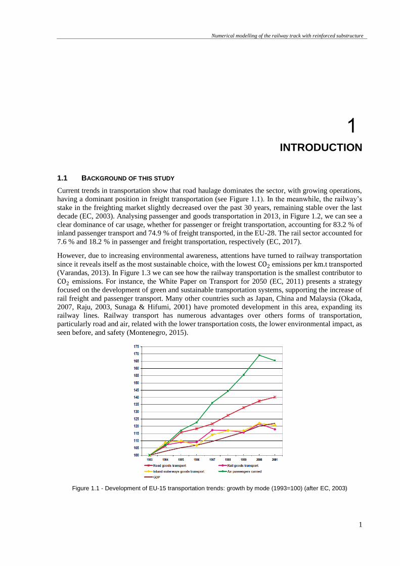
Current trends in transportation show that road haulage dominates the sector, with growing operations,
having a dominant position in freight transportation (see Figure 1.1). In the meanwhile, the railway’s
stake in the freighting market slightly decreased over the past 30 years, remaining stable over the last
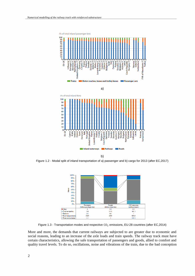
decade (EC, 2003). Analysing passenger and goods transportation in 2013, in Figure 1.2, we can see a
clear dominance of car usage, whether for passenger or freight transportation, accounting for 83.2 % of
inland passenger transport and 74.9 % of freight transported, in the EU-28. The rail sector accounted for
7.6 % and 18.2 % in passenger and freight transportation, respectively (EC, 2017).
However, due to increasing environmental awareness, attentions have turned to railway transportation
since it reveals itself as the most sustainable choice, with the lowest CO2 emissions per km.t transported
(Varandas, 2013). In Figure 1.3 we can see how the railway transportation is the smallest contributor to
CO2 emissions. For instance, the White Paper on Transport for 2050 (EC, 2011) presents a strategy
focused on the development of green and sustainable transportation systems, supporting the increase of
rail freight and passenger transport. Many other countries such as Japan, China and Malaysia (Okada,
2007, Raju, 2003, Sunaga & Hifumi, 2001) have promoted development in this area, expanding its
railway lines. Railway transport has numerous advantages over others forms of transportation,
particularly road and air, related with the lower transportation costs, the lower environmental impact, as
seen before, and safety (Montenegro, 2015).
Figure 1.1 - Development of EU-15 transportation trends: growth by mode (1993=100) (after EC, 2003)
Numerical modelling of the railway track with reinforced substructure
2
a)
b)
Figure 1.2 - Modal split of inland transportation of a) passenger and b) cargo for 2013 (after EC,2017)
Figure 1.3 - Transportation modes and respective CO2 emissions, EU-28 countries (after EC,2014)
More and more, the demands that current railways are subjected to are greater due to economic and
social reasons, leading to an increase of the axle loads and train speeds. The railway track must have
certain characteristics, allowing the safe transportation of passengers and goods, allied to comfort and
quality travel levels. To do so, oscillations, noise and vibrations of the train, due to the bad conception
Numerical modelling of the railway track with reinforced substructure
3
of the track system or due to degradation of it, must not exceed certain limits (Paixão, 2014). Despite
this, it is known that, throughout its life-cycle, the railway track degrades its quality (Selig & Waters,
1994). Nowadays, many railways struggle to meet the standards of a good quality track, since its design
is not appropriate nor the ground conditions are favourable (Ekberg & Paulsson, 2010). As demands for
railway transportation are becoming higher and traffic is growing, there is a need to upgrade these tracks
(Ekberg & Paulsson, 2010).
The main functions of the track are to guide the train correctly, to withstand the train’s loads and to
distribute that same load over a larger area as possible (Dahlberg, 2003), thus quickly reducing the
stresses developed into the track substructure (Profillidis, 2000).
Even though there are many design methods available to properly determine the granular layer thickness
of the rail track (Li & Selig, 1998), these granular materials suffer degradation, for instance, due to
stresses imposed by the cyclic axle loads transferred from the track components onto the subgrade (Selig
& Waters, 1994) or due to the weather conditions. To prevent this, a regular monitoring of the track
conditions (i.e. in terms of track geometric quality, fault detection and component degradation, among
other aspects) combined with adequate maintenance measures should be carried out in order to avoid
compromising the track’s correct functioning.
In general, the main causes behind track quality degradation are: i) the nature of the axle loads; ii) the
variation of the characteristics of the materials that compose the rail track and iii) the environmental
conditions (Fortunato, 2005, Ribeiro, Viviana 2015). From the causes mentioned above, the most severe
is the nature of the load due to its high value and cyclic nature (Fortunato, 2005). The long-term
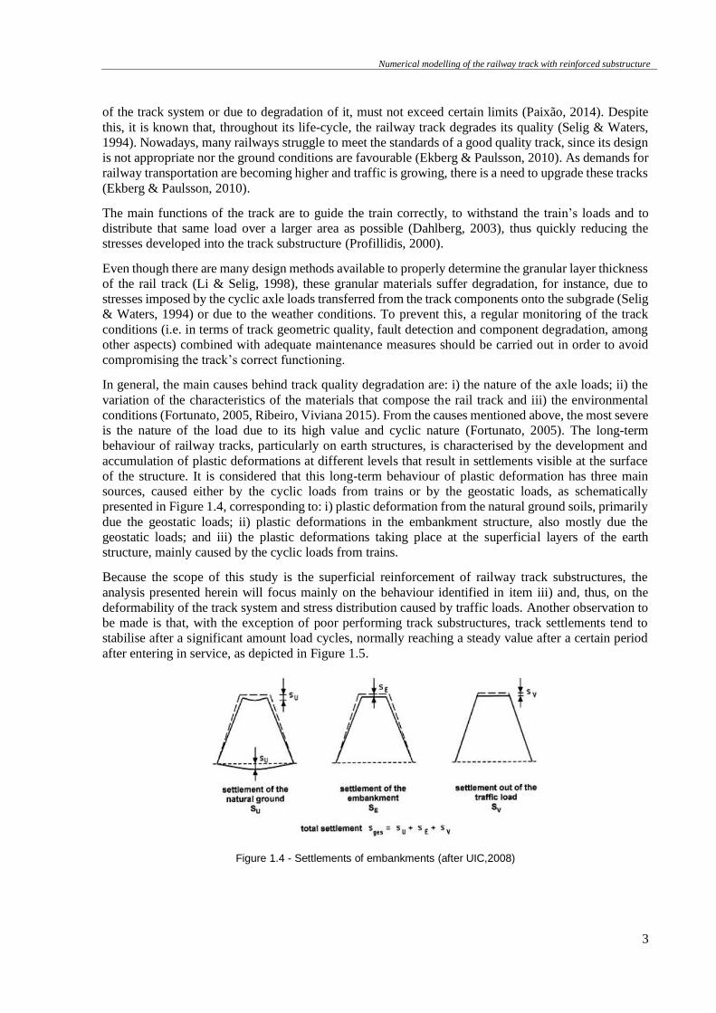
behaviour of railway tracks, particularly on earth structures, is characterised by the development and
accumulation of plastic deformations at different levels that result in settlements visible at the surface
of the structure. It is considered that this long-term behaviour of plastic deformation has three main
sources, caused either by the cyclic loads from trains or by the geostatic loads, as schematically
presented in Figure 1.4, corresponding to: i) plastic deformation from the natural ground soils, primarily
due the geostatic loads; ii) plastic deformations in the embankment structure, also mostly due the
geostatic loads; and iii) the plastic deformations taking place at the superficial layers of the earth
structure, mainly caused by the cyclic loads from trains.
Because the scope of this study is the superficial reinforcement of railway track substructures, the
analysis presented herein will focus mainly on the behaviour identified in item iii) and, thus, on the
deformability of the track system and stress distribution caused by traffic loads. Another observation to
be made is that, with the exception of poor performing track substructures, track settlements tend to
stabilise after a significant amount load cycles, normally reaching a steady value after a certain period
after entering in service, as depicted in Figure 1.5.
Figure 1.4 - Settlements of embankments (after UIC,2008)
Numerical modelling of the railway track with reinforced substructure
4
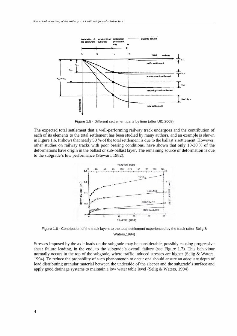
Figure 1.5 - Different settlement parts by time (after UIC,2008)
The expected total settlement that a well-performing railway track undergoes and the contribution of
each of its elements to the total settlement has been studied by many authors, and an example is shown
in Figure 1.6. It shows that nearly 50 % of the total settlement is due to the ballast’s settlement. However,
other studies on railway tracks with poor bearing conditions, have shown that only 10-30 % of the
deformations have origin in the ballast or sub-ballast layer. The remaining source of deformation is due
to the subgrade’s low performance (Stewart, 1982).
Figure 1.6 - Contribution of the track layers to the total settlement experienced by the track (after Selig &
Waters,1994)
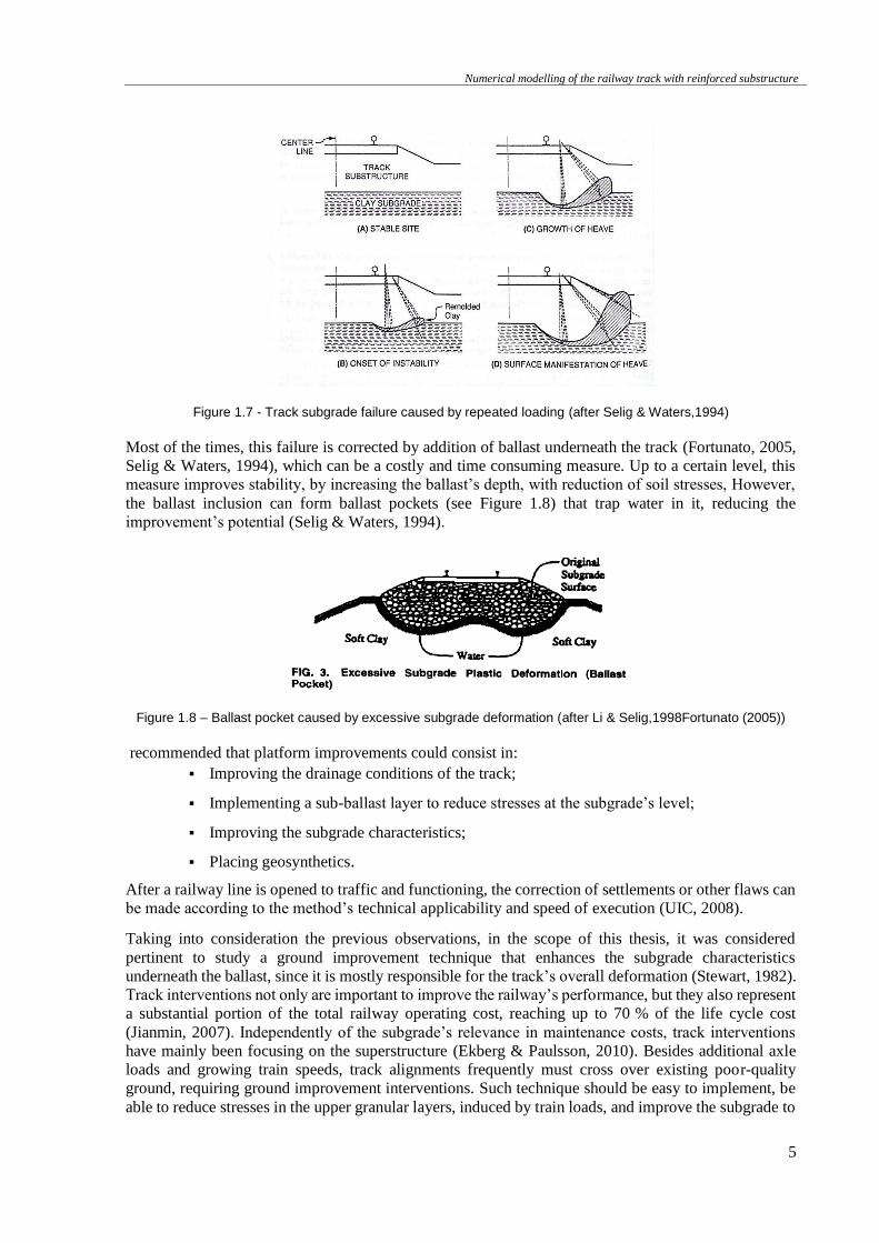
Stresses imposed by the axle loads on the subgrade may be considerable, possibly causing progressive
shear failure leading, in the end, to the subgrade’s overall failure (see Figure 1.7). This behaviour
normally occurs in the top of the subgrade, where traffic induced stresses are higher (Selig & Waters,
1994). To reduce the probability of such phenomenon to occur one should ensure an adequate depth of
load distributing granular material between the underside of the sleeper and the subgrade’s surface and
apply good drainage systems to maintain a low water table level (Selig & Waters, 1994).
Numerical modelling of the railway track with reinforced substructure
5
Figure 1.7 - Track subgrade failure caused by repeated loading (after Selig & Waters,1994)
Most of the times, this failure is corrected by addition of ballast underneath the track (Fortunato, 2005,
Selig & Waters, 1994), which can be a costly and time consuming measure. Up to a certain level, this
measure improves stability, by increasing the ballast’s depth, with reduction of soil stresses, However,
the ballast inclusion can form ballast pockets (see Figure 1.8) that trap water in it, reducing the
improvement’s potential (Selig & Waters, 1994).
Figure 1.8 – Ballast pocket caused by excessive subgrade deformation (after Li & Selig,1998Fortunato (2005))
recommended that platform improvements could consist in:
▪ Improving the drainage conditions of the track;
▪ Implementing a sub-ballast layer to reduce stresses at the subgrade’s level;
▪ Improving the subgrade characteristics;
▪ Placing geosynthetics.
After a railway line is opened to traffic and functioning, the correction of settlements or other flaws can
be made according to the method’s technical applicability and speed of execution (UIC, 2008).
Taking into consideration the previous observations, in the scope of this thesis, it was considered
pertinent to study a ground improvement technique that enhances the subgrade characteristics
underneath the ballast, since it is mostly responsible for the track’s overall deformation (Stewart, 1982).
Track interventions not only are important to improve the railway’s performance, but they also represent
a substantial portion of the total railway operating cost, reaching up to 70 % of the life cycle cost
(Jianmin, 2007). Independently of the subgrade’s relevance in maintenance costs, track interventions
have mainly been focusing on the superstructure (Ekberg & Paulsson, 2010). Besides additional axle
loads and growing train speeds, track alignments frequently must cross over existing poor-quality
ground, requiring ground improvement interventions. Such technique should be easy to implement, be
able to reduce stresses in the upper granular layers, induced by train loads, and improve the subgrade to
Numerical modelling of the railway track with reinforced substructure
6
achieve as closely as possible the behaviour represented in Figure 1.6. To do so, it was chosen to study
the efficiency of including short Jet-grout columns placed in various patterns, as will be described later
in more detail.
Recently, many studies and projects about track degradation have been developed with the purpose to
upgrade the tracks to current and higher standards. Example of such projects, where ground-
improvement interventions are exposed in various case studies, are the SUPERTRACK (2005),
INNOTRACK (2010), SMARTRAIL (2014) and RUFEX (2011).
The analysis made in this thesis focuses on structural behaviour of a railway track after being submitted
to substructure reinforcement with short columns. It is considered that the plastic deformation of the
studied structures is residual, thus evidencing a quasi-elastic behaviour.
1.2 AIM OF THIS STUDY
This thesis focus is to study and evaluate the track’s structural behaviour when its substructure is
improved with short Jet-grout columns. To do so, detailed three-dimensional FDM models, designed
with various layouts with different placement patterns of Jet-grout columns, will be studied. Parametric
studies on the influence of the column diameter, column pattern and loading position will be made,
considering two different material behaviour models for the ballast layer, and ultimately comparing
them.
The main expected contributions are not only to obtain more insight into the behaviour of these
structures and to assess the advantages and potentiality of this ground improvement technique, but also
to evaluate the impact of considering non-linear elastic constitutive behaviour for the ballast layer in
these advanced numerical modelling approaches.
1.3 THESIS OUTLINE
This thesis is made up by six chapters.
In Chapter 2, a general description of the ballasted track system and its components is made followed
by a brief state of the art regarding soil improvement techniques, with application to railways. The
methods exposed include the application of geosynthetics, vibro-techniques and grouting techniques.
In Chapter 3, a series of parametric numerical studies regarding interfaces, using FLAC3D, are analysed
due to the existence, in the railway model, of certain important interactions that require accurate
modelling, such as the sleeper/ballast interaction. In the first parametric study, the implications of
applying an interface and how to model its behaviour was assessed. The second parametric test aimed
to study the interaction between different mesh types. These parametric tests were made in simpler and
smaller models, compared with the railway track models in the following chapters. Ultimately, a
conclusion is reached on which software command to apply to the larger scale railway model.
In Chapter 4, a general description of the designed railway numerical models is made, detailing material
characteristics, modelling procedures, assigned material constitutive behaviours and other details.
In Chapter 5, to obtain more insight into the behaviour of tracks improved by Jet-grout columns and to
assess the advantages and potentiality of this ground improvement technique, the results of parametric
studies regarding the influence of the column diameter, column pattern and loading position, in terms
of vertical stress and displacement, are presented and discussed. Since one of the focuses of this study
was to see the influence of implementing a non-linear elastic behaviour to the ballast layer, in the end
of this chapter a comparison between linear elastic and non-linear elastic behaviour is established. Due
to the extent of these parametric studies, a limited number of results and plots are presented in this
chapter, being the remaining results presented in the digital annexes.
Lastly, in Chapter 6, the main conclusions and recommendations for future developments are mentioned.

Numerical modelling of the railway track with reinforced substructure
7

Numerical modelling of the railway track with reinforced substructure
8

Numerical modelling of the railway track with reinforced substructure
9
THE TRACK SYSTEM AND SOIL
IMPROVEMENT TECHNIQUES FOR RAILWAY TRACKS
2.1 INTRODUCTION
Currently, many railways still consist of old conventional lines where, for the most part, its design is not
optimized and the subgrade is of low quality. Throughout the years, maintenance and inspections were
targeted to the superstructure, neglecting the subgrade, regardless of its importance in the track
maintenance costs (Ekberg & Paulsson, 2010).
As standards for railway transportation are becoming more demanding and traffic is increasing, there is
a need to upgrade these tracks, applying diverse types of improvements, therefore increasing the quality
and capacity of these rail lines. Subgrade improvement techniques should consider the current conditions
of the track, the desirable outcome for track performance under traffic, economic impact and experience
of the railway company. These methods’ range is wide, extending from some meters to several
kilometres of applicability, depending on the technique (Ekberg & Paulsson, 2010).
However, ground improvement techniques are very-costly, including materials, labour and traffic
interruptions that can be extensive in time. Thereby, there is a need to find ground improvement methods
that are cost efficient. But these methods must be verified thoroughly before being applied in actual
railway tracks. This is where the importance of numerical methods steps in, justifying one of the
purposes of this thesis. With numerical methods, it is possible to simulate the behaviour of certain
subgrade improvement technique, predicting its behaviour before applying it in the railway line.
Nevertheless, experimental field research is also very important to confirm numerical simulations
(Ekberg & Paulsson, 2010).
In this chapter, the general composition of the ballasted track system is detailed followed by a general
overview of some soil improvement techniques. These methods can be classified in two main categories:
mechanical and chemical methods. Mechanical methods include geosynthetics, vibro-techniques, jet-
grouting, deep soil mixing and micro pile installation. Chemical methods are electro-osmosis and
chemical grouts. Only the mechanical methods are explained in this chapter, for a briefer overview.
2.2 THE TRACK SYSTEM COMPOSITION
To the purpose of this thesis, only the composition of the ballasted track system will be detailed,
presenting the most common configuration of this structure and the function of its components. However
other track configurations exist such as the slab track (Fortunato & Paixão, 2009). In Figure 2.1 a
schematic representation of the difference between a ballastless and a ballasted track is shown.
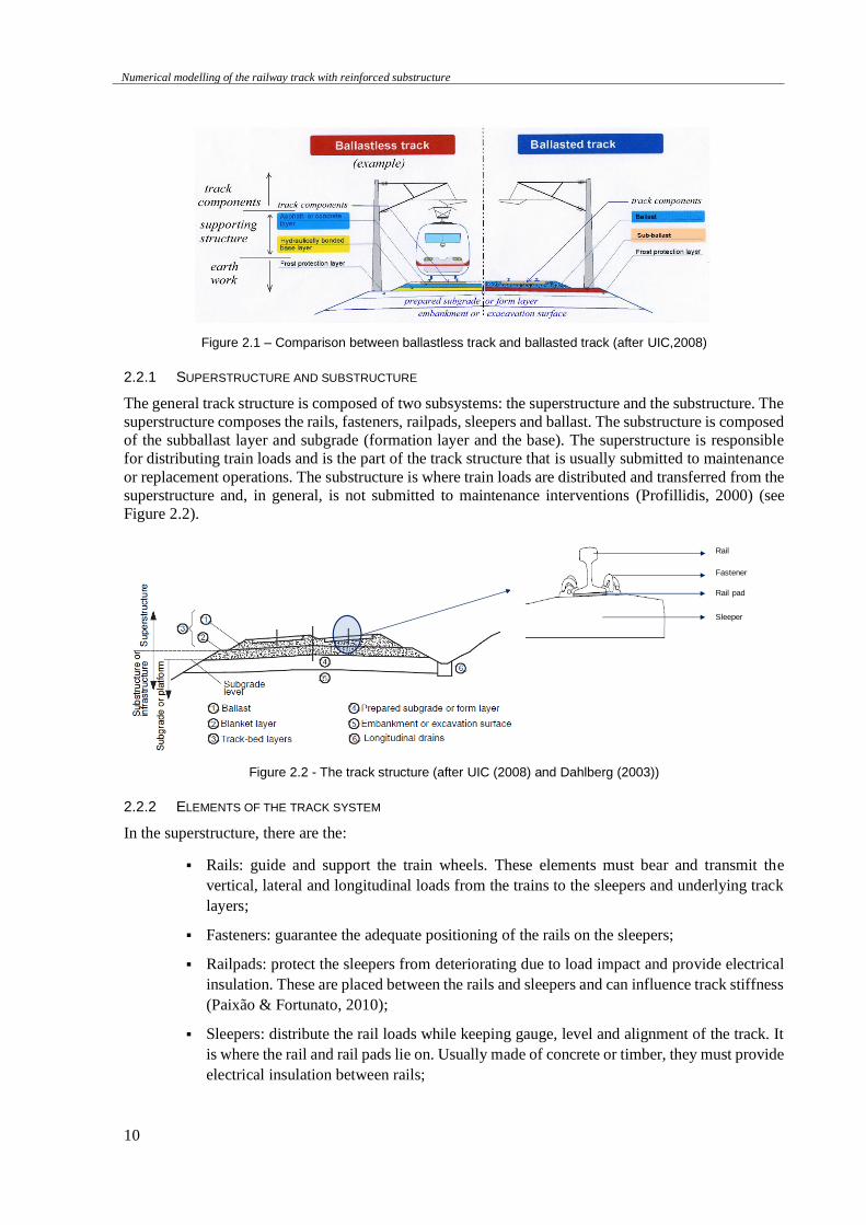
Numerical modelling of the railway track with reinforced substructure
10
Figure 2.1 – Comparison between ballastless track and ballasted track (after UIC,2008)
2.2.1 SUPERSTRUCTURE AND SUBSTRUCTURE
The general track structure is composed of two subsystems: the superstructure and the substructure. The
superstructure composes the rails, fasteners, railpads, sleepers and ballast. The substructure is composed
of the subballast layer and subgrade (formation layer and the base). The superstructure is responsible
for distributing train loads and is the part of the track structure that is usually submitted to maintenance
or replacement operations. The substructure is where train loads are distributed and transferred from the
superstructure and, in general, is not submitted to maintenance interventions (Profillidis, 2000) (see
Figure 2.2).
Figure 2.2 - The track structure (after UIC (2008) and Dahlberg (2003))
2.2.2 ELEMENTS OF THE TRACK SYSTEM
In the superstructure, there are the:
▪ Rails: guide and support the train wheels. These elements must bear and transmit the
vertical, lateral and longitudinal loads from the trains to the sleepers and underlying track
layers;
▪ Fasteners: guarantee the adequate positioning of the rails on the sleepers;
▪ Railpads: protect the sleepers from deteriorating due to load impact and provide electrical
insulation. These are placed between the rails and sleepers and can influence track stiffness
(Paixão & Fortunato, 2010);
▪ Sleepers: distribute the rail loads while keeping gauge, level and alignment of the track. It
is where the rail and rail pads lie on. Usually made of concrete or timber, they must provide
electrical insulation between rails;
Rail
Fastener
Rail pad
Sleeper
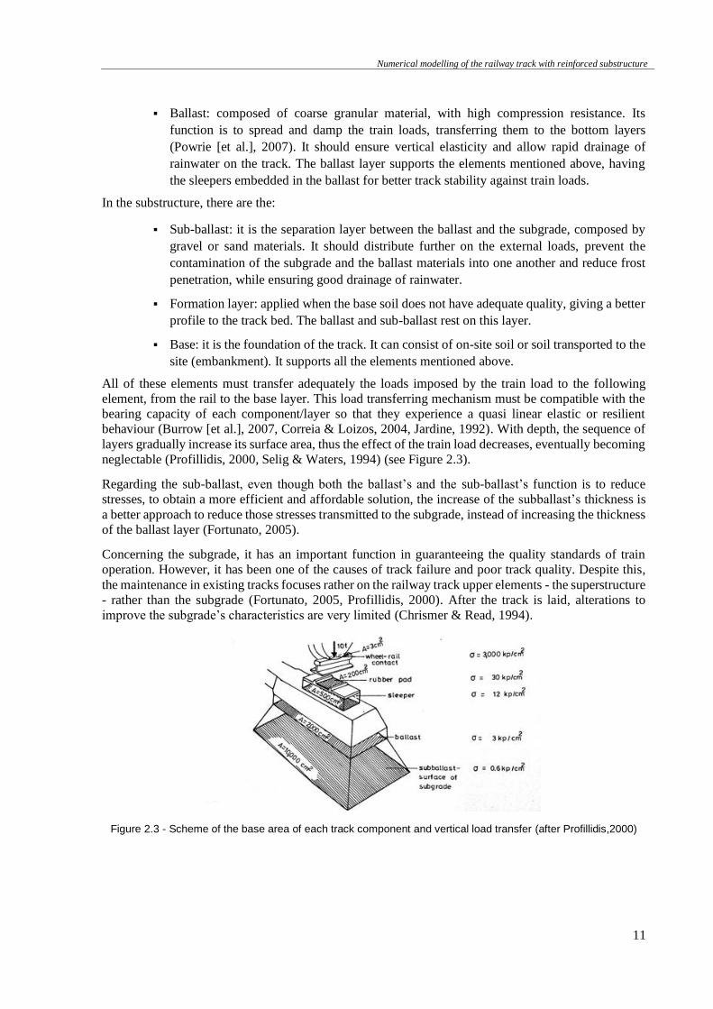
Numerical modelling of the railway track with reinforced substructure
11
▪ Ballast: composed of coarse granular material, with high compression resistance. Its
function is to spread and damp the train loads, transferring them to the bottom layers
(Powrie [et al.], 2007). It should ensure vertical elasticity and allow rapid drainage of
rainwater on the track. The ballast layer supports the elements mentioned above, having
the sleepers embedded in the ballast for better track stability against train loads.
In the substructure, there are the:
▪ Sub-ballast: it is the separation layer between the ballast and the subgrade, composed by
gravel or sand materials. It should distribute further on the external loads, prevent the
contamination of the subgrade and the ballast materials into one another and reduce frost
penetration, while ensuring good drainage of rainwater.
▪ Formation layer: applied when the base soil does not have adequate quality, giving a better
profile to the track bed. The ballast and sub-ballast rest on this layer.
▪ Base: it is the foundation of the track. It can consist of on-site soil or soil transported to the
site (embankment). It supports all the elements mentioned above.
All of these elements must transfer adequately the loads imposed by the train load to the following
element, from the rail to the base layer. This load transferring mechanism must be compatible with the
bearing capacity of each component/layer so that they experience a quasi linear elastic or resilient
behaviour (Burrow [et al.], 2007, Correia & Loizos, 2004, Jardine, 1992). With depth, the sequence of
layers gradually increase its surface area, thus the effect of the train load decreases, eventually becoming
neglectable (Profillidis, 2000, Selig & Waters, 1994) (see Figure 2.3).
Regarding the sub-ballast, even though both the ballast’s and the sub-ballast’s function is to reduce
stresses, to obtain a more efficient and affordable solution, the increase of the subballast’s thickness is
a better approach to reduce those stresses transmitted to the subgrade, instead of increasing the thickness
of the ballast layer (Fortunato, 2005).
Concerning the subgrade, it has an important function in guaranteeing the quality standards of train
operation. However, it has been one of the causes of track failure and poor track quality. Despite this,
the maintenance in existing tracks focuses rather on the railway track upper elements - the superstructure
- rather than the subgrade (Fortunato, 2005, Profillidis, 2000). After the track is laid, alterations to
improve the subgrade’s characteristics are very limited (Chrismer & Read, 1994).
Figure 2.3 - Scheme of the base area of each track component and vertical load transfer (after Profillidis,2000)
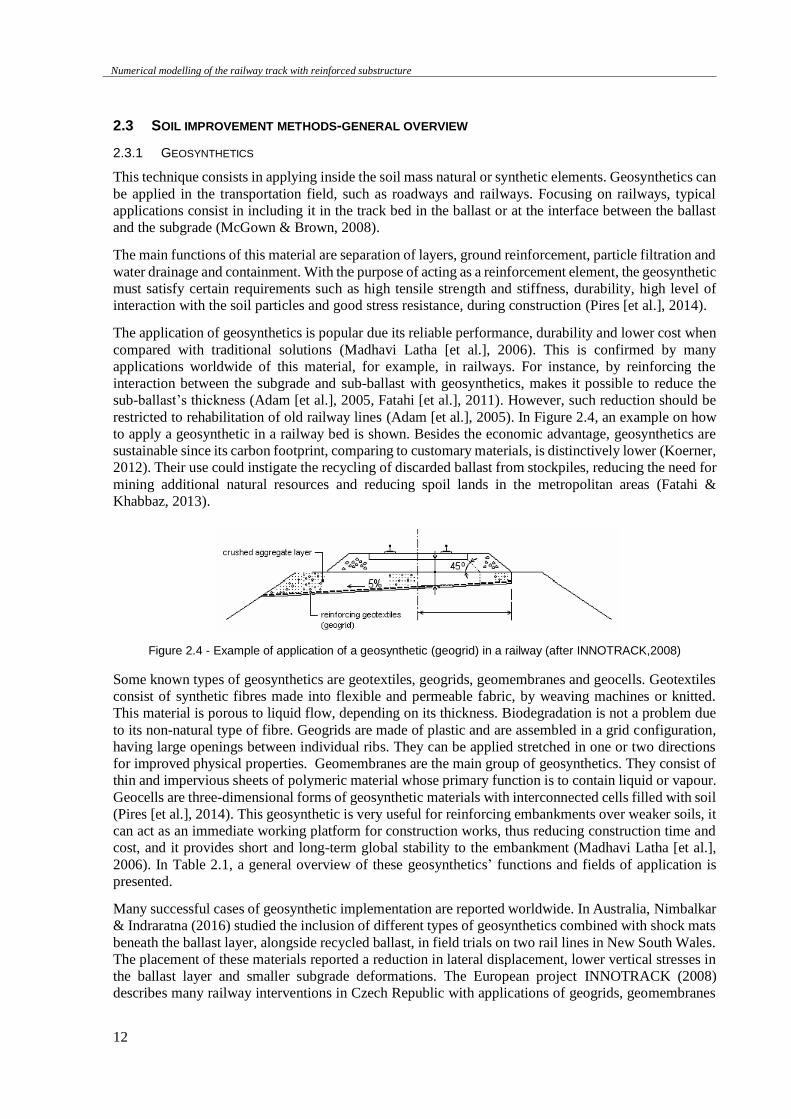
Numerical modelling of the railway track with reinforced substructure
12
2.3 SOIL IMPROVEMENT METHODS-GENERAL OVERVIEW
2.3.1 GEOSYNTHETICS
This technique consists in applying inside the soil mass natural or synthetic elements. Geosynthetics can
be applied in the transportation field, such as roadways and railways. Focusing on railways, typical
applications consist in including it in the track bed in the ballast or at the interface between the ballast
and the subgrade (McGown & Brown, 2008).
The main functions of this material are separation of layers, ground reinforcement, particle filtration and
water drainage and containment. With the purpose of acting as a reinforcement element, the geosynthetic
must satisfy certain requirements such as high tensile strength and stiffness, durability, high level of
interaction with the soil particles and good stress resistance, during construction (Pires [et al.], 2014).
The application of geosynthetics is popular due its reliable performance, durability and lower cost when
compared with traditional solutions (Madhavi Latha [et al.], 2006). This is confirmed by many
applications worldwide of this material, for example, in railways. For instance, by reinforcing the
interaction between the subgrade and sub-ballast with geosynthetics, makes it possible to reduce the
sub-ballast’s thickness (Adam [et al.], 2005, Fatahi [et al.], 2011). However, such reduction should be
restricted to rehabilitation of old railway lines (Adam [et al.], 2005). In Figure 2.4, an example on how
to apply a geosynthetic in a railway bed is shown. Besides the economic advantage, geosynthetics are
sustainable since its carbon footprint, comparing to customary materials, is distinctively lower (Koerner,
2012). Their use could instigate the recycling of discarded ballast from stockpiles, reducing the need for
mining additional natural resources and reducing spoil lands in the metropolitan areas (Fatahi &
Khabbaz, 2013).
Figure 2.4 - Example of application of a geosynthetic (geogrid) in a railway (after INNOTRACK,2008)
Some known types of geosynthetics are geotextiles, geogrids, geomembranes and geocells. Geotextiles
consist of synthetic fibres made into flexible and permeable fabric, by weaving machines or knitted.
This material is porous to liquid flow, depending on its thickness. Biodegradation is not a problem due
to its non-natural type of fibre. Geogrids are made of plastic and are assembled in a grid configuration,
having large openings between individual ribs. They can be applied stretched in one or two directions
for improved physical properties. Geomembranes are the main group of geosynthetics. They consist of
thin and impervious sheets of polymeric material whose primary function is to contain liquid or vapour.
Geocells are three-dimensional forms of geosynthetic materials with interconnected cells filled with soil
(Pires [et al.], 2014). This geosynthetic is very useful for reinforcing embankments over weaker soils, it
can act as an immediate working platform for construction works, thus reducing construction time and
cost, and it provides short and long-term global stability to the embankment (Madhavi Latha [et al.],
2006). In Table 2.1, a general overview of these geosynthetics’ functions and fields of application is
presented.
Many successful cases of geosynthetic implementation are reported worldwide. In Australia, Nimbalkar
& Indraratna (2016) studied the inclusion of different types of geosynthetics combined with shock mats
beneath the ballast layer, alongside recycled ballast, in field trials on two rail lines in New South Wales.
The placement of these materials reported a reduction in lateral displacement, lower vertical stresses in
the ballast layer and smaller subgrade deformations. The European project INNOTRACK (2008)
describes many railway interventions in Czech Republic with applications of geogrids, geomembranes
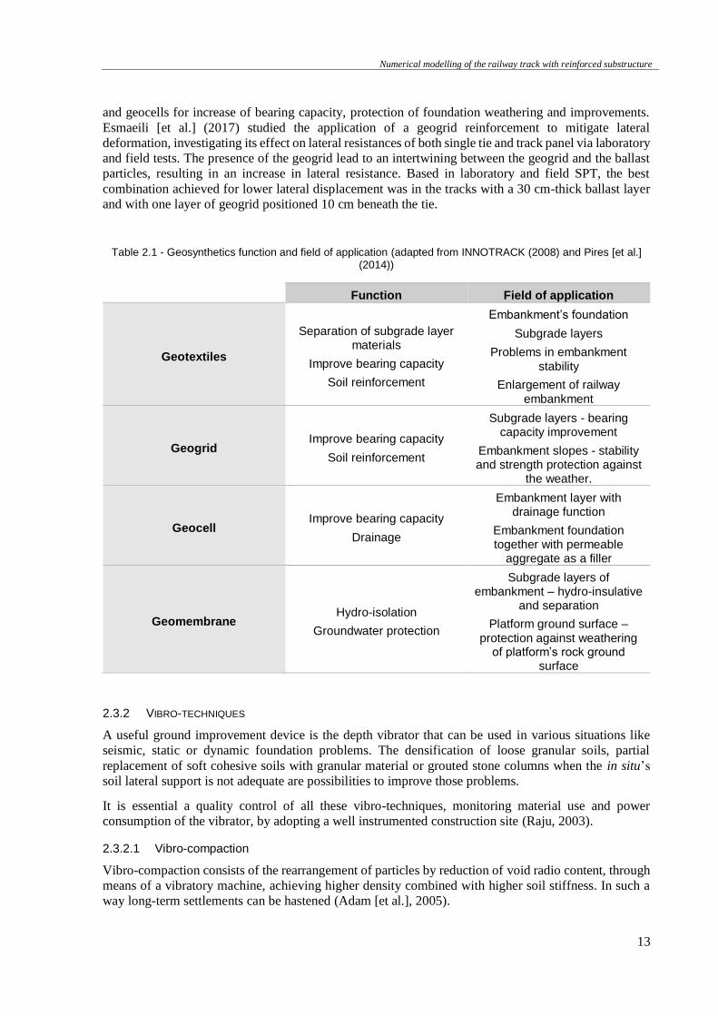
Numerical modelling of the railway track with reinforced substructure
13
and geocells for increase of bearing capacity, protection of foundation weathering and improvements.
Esmaeili [et al.] (2017) studied the application of a geogrid reinforcement to mitigate lateral
deformation, investigating its effect on lateral resistances of both single tie and track panel via laboratory
and field tests. The presence of the geogrid lead to an intertwining between the geogrid and the ballast
particles, resulting in an increase in lateral resistance. Based in laboratory and field SPT, the best
combination achieved for lower lateral displacement was in the tracks with a 30 cm-thick ballast layer
and with one layer of geogrid positioned 10 cm beneath the tie.
Table 2.1 - Geosynthetics function and field of application (adapted from INNOTRACK (2008) and Pires [et al.] (2014))
Function Field of application
Geotextiles
Separation of subgrade layer materials
Improve bearing capacity
Soil reinforcement
Embankment’s foundation
Subgrade layers
Problems in embankment
stability
Enlargement of railway
embankment
Geogrid Improve bearing capacity
Soil reinforcement
Subgrade layers - bearing capacity improvement
Embankment slopes - stability and strength protection against
the weather.
Geocell Improve bearing capacity
Drainage
Embankment layer with drainage function
Embankment foundation together with permeable
aggregate as a filler
Geomembrane Hydro-isolation
Groundwater protection
Subgrade layers of embankment – hydro-insulative
and separation
Platform ground surface –
protection against weathering of platform’s rock ground
surface
2.3.2 VIBRO-TECHNIQUES
A useful ground improvement device is the depth vibrator that can be used in various situations like
seismic, static or dynamic foundation problems. The densification of loose granular soils, partial
replacement of soft cohesive soils with granular material or grouted stone columns when the in situ’s
soil lateral support is not adequate are possibilities to improve those problems.
It is essential a quality control of all these vibro-techniques, monitoring material use and power
consumption of the vibrator, by adopting a well instrumented construction site (Raju, 2003).
2.3.2.1 Vibro-compaction
Vibro-compaction consists of the rearrangement of particles by reduction of void radio content, through
means of a vibratory machine, achieving higher density combined with higher soil stiffness. In such a
way long-term settlements can be hastened (Adam [et al.], 2005).
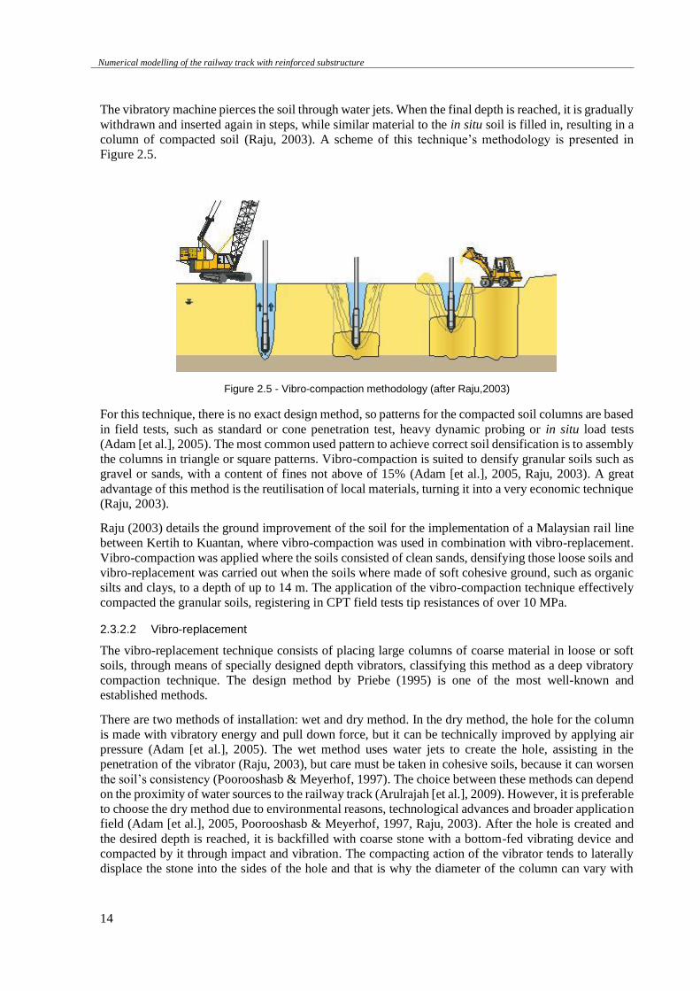
Numerical modelling of the railway track with reinforced substructure
14
The vibratory machine pierces the soil through water jets. When the final depth is reached, it is gradually
withdrawn and inserted again in steps, while similar material to the in situ soil is filled in, resulting in a
column of compacted soil (Raju, 2003). A scheme of this technique’s methodology is presented in
Figure 2.5.
Figure 2.5 - Vibro-compaction methodology (after Raju,2003)
For this technique, there is no exact design method, so patterns for the compacted soil columns are based
in field tests, such as standard or cone penetration test, heavy dynamic probing or in situ load tests
(Adam [et al.], 2005). The most common used pattern to achieve correct soil densification is to assembly
the columns in triangle or square patterns. Vibro-compaction is suited to densify granular soils such as
gravel or sands, with a content of fines not above of 15% (Adam [et al.], 2005, Raju, 2003). A great
advantage of this method is the reutilisation of local materials, turning it into a very economic technique
(Raju, 2003).
Raju (2003) details the ground improvement of the soil for the implementation of a Malaysian rail line
between Kertih to Kuantan, where vibro-compaction was used in combination with vibro-replacement.
Vibro-compaction was applied where the soils consisted of clean sands, densifying those loose soils and
vibro-replacement was carried out when the soils where made of soft cohesive ground, such as organic
silts and clays, to a depth of up to 14 m. The application of the vibro-compaction technique effectively
compacted the granular soils, registering in CPT field tests tip resistances of over 10 MPa.
2.3.2.2 Vibro-replacement
The vibro-replacement technique consists of placing large columns of coarse material in loose or soft
soils, through means of specially designed depth vibrators, classifying this method as a deep vibratory
compaction technique. The design method by Priebe (1995) is one of the most well-known and
established methods.
There are two methods of installation: wet and dry method. In the dry method, the hole for the column
is made with vibratory energy and pull down force, but it can be technically improved by applying air
pressure (Adam [et al.], 2005). The wet method uses water jets to create the hole, assisting in the
penetration of the vibrator (Raju, 2003), but care must be taken in cohesive soils, because it can worsen
the soil’s consistency (Poorooshasb & Meyerhof, 1997). The choice between these methods can depend
on the proximity of water sources to the railway track (Arulrajah [et al.], 2009). However, it is preferable
to choose the dry method due to environmental reasons, technological advances and broader application
field (Adam [et al.], 2005, Poorooshasb & Meyerhof, 1997, Raju, 2003). After the hole is created and
the desired depth is reached, it is backfilled with coarse stone with a bottom-fed vibrating device and
compacted by it through impact and vibration. The compacting action of the vibrator tends to laterally
displace the stone into the sides of the hole and that is why the diameter of the column can vary with
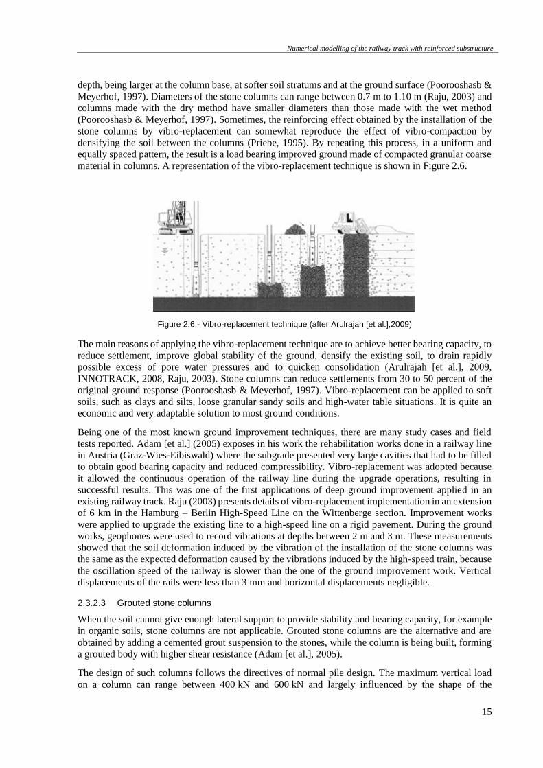
Numerical modelling of the railway track with reinforced substructure
15
depth, being larger at the column base, at softer soil stratums and at the ground surface (Poorooshasb &
Meyerhof, 1997). Diameters of the stone columns can range between 0.7 m to 1.10 m (Raju, 2003) and
columns made with the dry method have smaller diameters than those made with the wet method
(Poorooshasb & Meyerhof, 1997). Sometimes, the reinforcing effect obtained by the installation of the
stone columns by vibro-replacement can somewhat reproduce the effect of vibro-compaction by
densifying the soil between the columns (Priebe, 1995). By repeating this process, in a uniform and
equally spaced pattern, the result is a load bearing improved ground made of compacted granular coarse
material in columns. A representation of the vibro-replacement technique is shown in Figure 2.6.
Figure 2.6 - Vibro-replacement technique (after Arulrajah [et al.],2009)
The main reasons of applying the vibro-replacement technique are to achieve better bearing capacity, to
reduce settlement, improve global stability of the ground, densify the existing soil, to drain rapidly
possible excess of pore water pressures and to quicken consolidation (Arulrajah [et al.], 2009,
INNOTRACK, 2008, Raju, 2003). Stone columns can reduce settlements from 30 to 50 percent of the
original ground response (Poorooshasb & Meyerhof, 1997). Vibro-replacement can be applied to soft
soils, such as clays and silts, loose granular sandy soils and high-water table situations. It is quite an
economic and very adaptable solution to most ground conditions.
Being one of the most known ground improvement techniques, there are many study cases and field
tests reported. Adam [et al.] (2005) exposes in his work the rehabilitation works done in a railway line
in Austria (Graz-Wies-Eibiswald) where the subgrade presented very large cavities that had to be filled
to obtain good bearing capacity and reduced compressibility. Vibro-replacement was adopted because
it allowed the continuous operation of the railway line during the upgrade operations, resulting in
successful results. This was one of the first applications of deep ground improvement applied in an
existing railway track. Raju (2003) presents details of vibro-replacement implementation in an extension
of 6 km in the Hamburg – Berlin High-Speed Line on the Wittenberge section. Improvement works
were applied to upgrade the existing line to a high-speed line on a rigid pavement. During the ground
works, geophones were used to record vibrations at depths between 2 m and 3 m. These measurements
showed that the soil deformation induced by the vibration of the installation of the stone columns was
the same as the expected deformation caused by the vibrations induced by the high-speed train, because
the oscillation speed of the railway is slower than the one of the ground improvement work. Vertical
displacements of the rails were less than 3 mm and horizontal displacements negligible.
2.3.2.3 Grouted stone columns
When the soil cannot give enough lateral support to provide stability and bearing capacity, for example
in organic soils, stone columns are not applicable. Grouted stone columns are the alternative and are
obtained by adding a cemented grout suspension to the stones, while the column is being built, forming
a grouted body with higher shear resistance (Adam [et al.], 2005).
The design of such columns follows the directives of normal pile design. The maximum vertical load
on a column can range between 400 kN and 600 kN and largely influenced by the shape of the
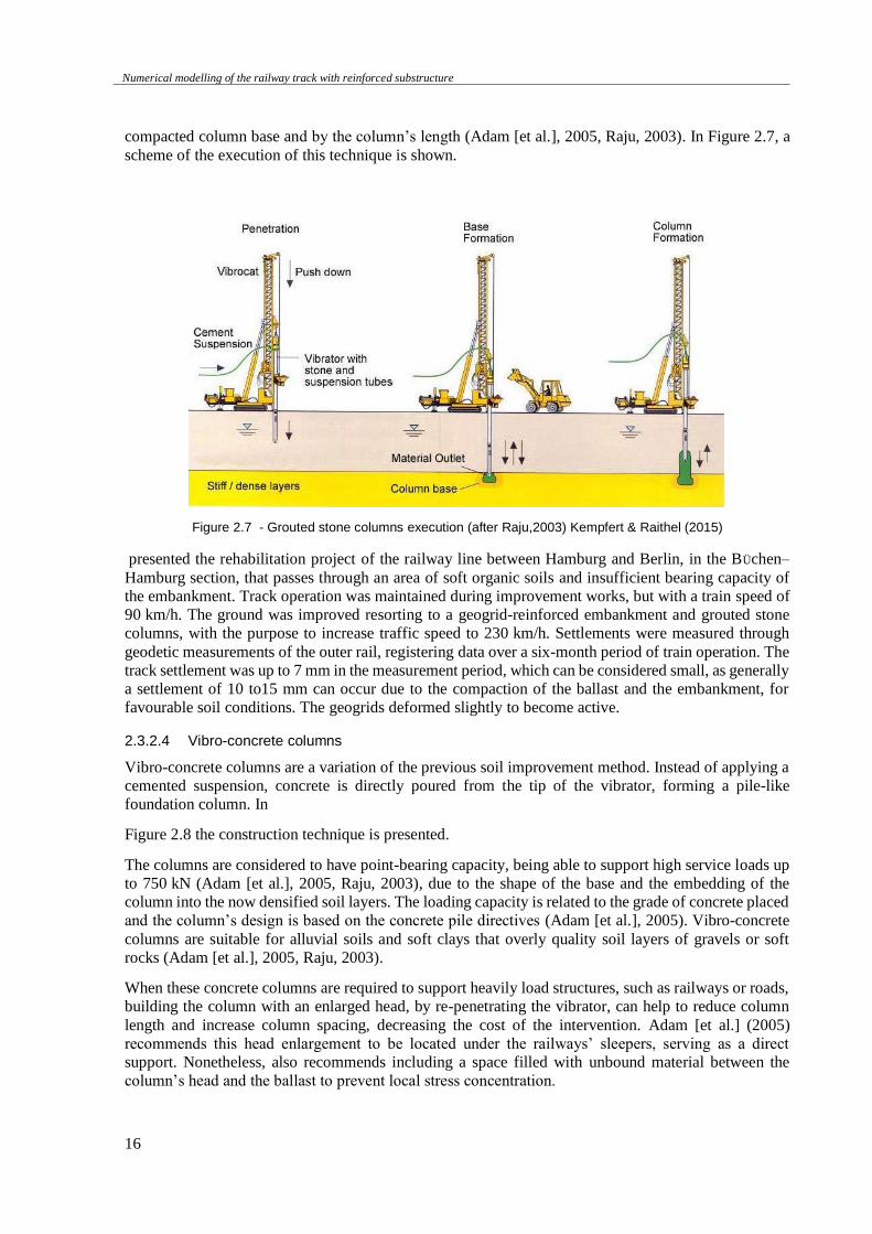
Numerical modelling of the railway track with reinforced substructure
16
compacted column base and by the column’s length (Adam [et al.], 2005, Raju, 2003). In Figure 2.7, a
scheme of the execution of this technique is shown.
Figure 2.7 - Grouted stone columns execution (after Raju,2003) Kempfert & Raithel (2015)
presented the rehabilitation project of the railway line between Hamburg and Berlin, in the BÜchen–
Hamburg section, that passes through an area of soft organic soils and insufficient bearing capacity of
the embankment. Track operation was maintained during improvement works, but with a train speed of
90 km/h. The ground was improved resorting to a geogrid-reinforced embankment and grouted stone
columns, with the purpose to increase traffic speed to 230 km/h. Settlements were measured through
geodetic measurements of the outer rail, registering data over a six-month period of train operation. The
track settlement was up to 7 mm in the measurement period, which can be considered small, as generally
a settlement of 10 to15 mm can occur due to the compaction of the ballast and the embankment, for
favourable soil conditions. The geogrids deformed slightly to become active.
2.3.2.4 Vibro-concrete columns
Vibro-concrete columns are a variation of the previous soil improvement method. Instead of applying a
cemented suspension, concrete is directly poured from the tip of the vibrator, forming a pile-like
foundation column. In
Figure 2.8 the construction technique is presented.
The columns are considered to have point-bearing capacity, being able to support high service loads up
to 750 kN (Adam [et al.], 2005, Raju, 2003), due to the shape of the base and the embedding of the
column into the now densified soil layers. The loading capacity is related to the grade of concrete placed
and the column’s design is based on the concrete pile directives (Adam [et al.], 2005). Vibro-concrete
columns are suitable for alluvial soils and soft clays that overly quality soil layers of gravels or soft
rocks (Adam [et al.], 2005, Raju, 2003).
When these concrete columns are required to support heavily load structures, such as railways or roads,
building the column with an enlarged head, by re-penetrating the vibrator, can help to reduce column
length and increase column spacing, decreasing the cost of the intervention. Adam [et al.] (2005)
recommends this head enlargement to be located under the railways’ sleepers, serving as a direct
support. Nonetheless, also recommends including a space filled with unbound material between the
column’s head and the ballast to prevent local stress concentration.
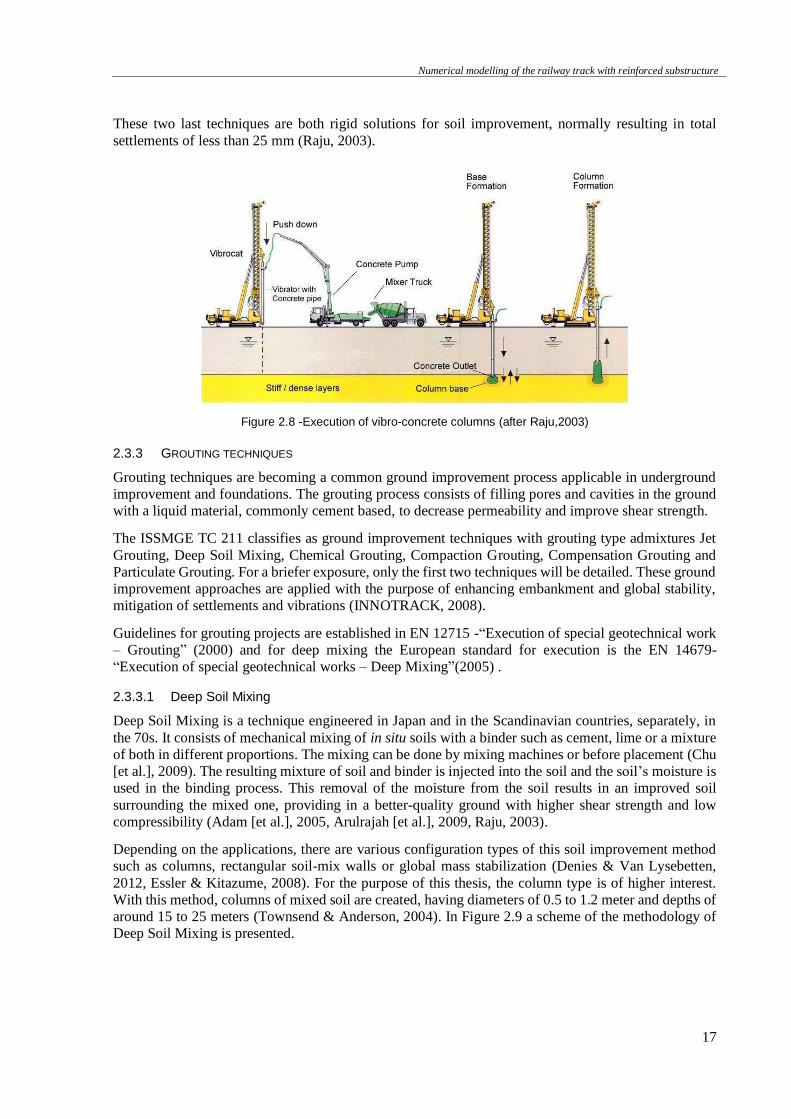
Numerical modelling of the railway track with reinforced substructure
17
These two last techniques are both rigid solutions for soil improvement, normally resulting in total
settlements of less than 25 mm (Raju, 2003).
Figure 2.8 -Execution of vibro-concrete columns (after Raju,2003)
2.3.3 GROUTING TECHNIQUES
Grouting techniques are becoming a common ground improvement process applicable in underground
improvement and foundations. The grouting process consists of filling pores and cavities in the ground
with a liquid material, commonly cement based, to decrease permeability and improve shear strength.
The ISSMGE TC 211 classifies as ground improvement techniques with grouting type admixtures Jet
Grouting, Deep Soil Mixing, Chemical Grouting, Compaction Grouting, Compensation Grouting and
Particulate Grouting. For a briefer exposure, only the first two techniques will be detailed. These ground
improvement approaches are applied with the purpose of enhancing embankment and global stability,
mitigation of settlements and vibrations (INNOTRACK, 2008).
Guidelines for grouting projects are established in EN 12715 -“Execution of special geotechnical work
– Grouting” (2000) and for deep mixing the European standard for execution is the EN 14679-
“Execution of special geotechnical works – Deep Mixing”(2005) .
2.3.3.1 Deep Soil Mixing
Deep Soil Mixing is a technique engineered in Japan and in the Scandinavian countries, separately, in
the 70s. It consists of mechanical mixing of in situ soils with a binder such as cement, lime or a mixture
of both in different proportions. The mixing can be done by mixing machines or before placement (Chu
[et al.], 2009). The resulting mixture of soil and binder is injected into the soil and the soil’s moisture is
used in the binding process. This removal of the moisture from the soil results in an improved soil
surrounding the mixed one, providing in a better-quality ground with higher shear strength and low
compressibility (Adam [et al.], 2005, Arulrajah [et al.], 2009, Raju, 2003).
Depending on the applications, there are various configuration types of this soil improvement method
such as columns, rectangular soil-mix walls or global mass stabilization (Denies & Van Lysebetten,
2012, Essler & Kitazume, 2008). For the purpose of this thesis, the column type is of higher interest.
With this method, columns of mixed soil are created, having diameters of 0.5 to 1.2 meter and depths of
around 15 to 25 meters (Townsend & Anderson, 2004). In Figure 2.9 a scheme of the methodology of
Deep Soil Mixing is presented.
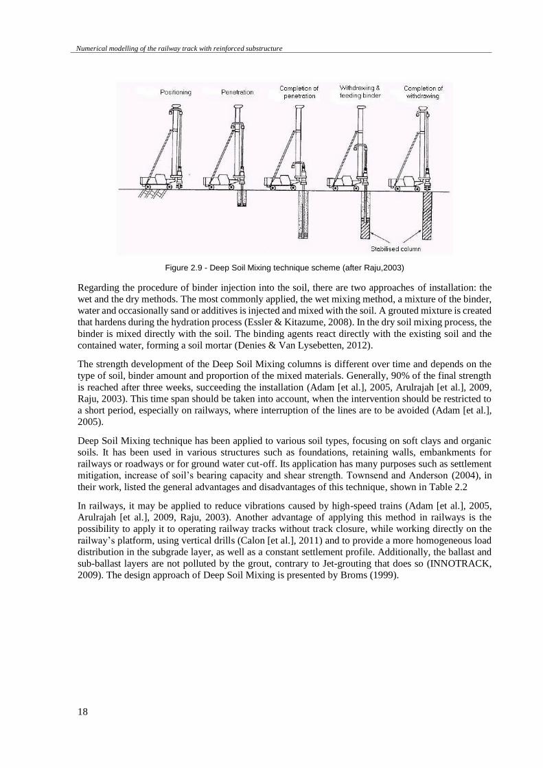
Numerical modelling of the railway track with reinforced substructure
18
Figure 2.9 - Deep Soil Mixing technique scheme (after Raju,2003)
Regarding the procedure of binder injection into the soil, there are two approaches of installation: the
wet and the dry methods. The most commonly applied, the wet mixing method, a mixture of the binder,
water and occasionally sand or additives is injected and mixed with the soil. A grouted mixture is created
that hardens during the hydration process (Essler & Kitazume, 2008). In the dry soil mixing process, the
binder is mixed directly with the soil. The binding agents react directly with the existing soil and the
contained water, forming a soil mortar (Denies & Van Lysebetten, 2012).
The strength development of the Deep Soil Mixing columns is different over time and depends on the
type of soil, binder amount and proportion of the mixed materials. Generally, 90% of the final strength
is reached after three weeks, succeeding the installation (Adam [et al.], 2005, Arulrajah [et al.], 2009,
Raju, 2003). This time span should be taken into account, when the intervention should be restricted to
a short period, especially on railways, where interruption of the lines are to be avoided (Adam [et al.],
2005).
Deep Soil Mixing technique has been applied to various soil types, focusing on soft clays and organic
soils. It has been used in various structures such as foundations, retaining walls, embankments for
railways or roadways or for ground water cut-off. Its application has many purposes such as settlement
mitigation, increase of soil’s bearing capacity and shear strength. Townsend and Anderson (2004), in
their work, listed the general advantages and disadvantages of this technique, shown in Table 2.2
In railways, it may be applied to reduce vibrations caused by high-speed trains (Adam [et al.], 2005,
Arulrajah [et al.], 2009, Raju, 2003). Another advantage of applying this method in railways is the
possibility to apply it to operating railway tracks without track closure, while working directly on the
railway’s platform, using vertical drills (Calon [et al.], 2011) and to provide a more homogeneous load
distribution in the subgrade layer, as well as a constant settlement profile. Additionally, the ballast and
sub-ballast layers are not polluted by the grout, contrary to Jet-grouting that does so (INNOTRACK,
2009). The design approach of Deep Soil Mixing is presented by Broms (1999).
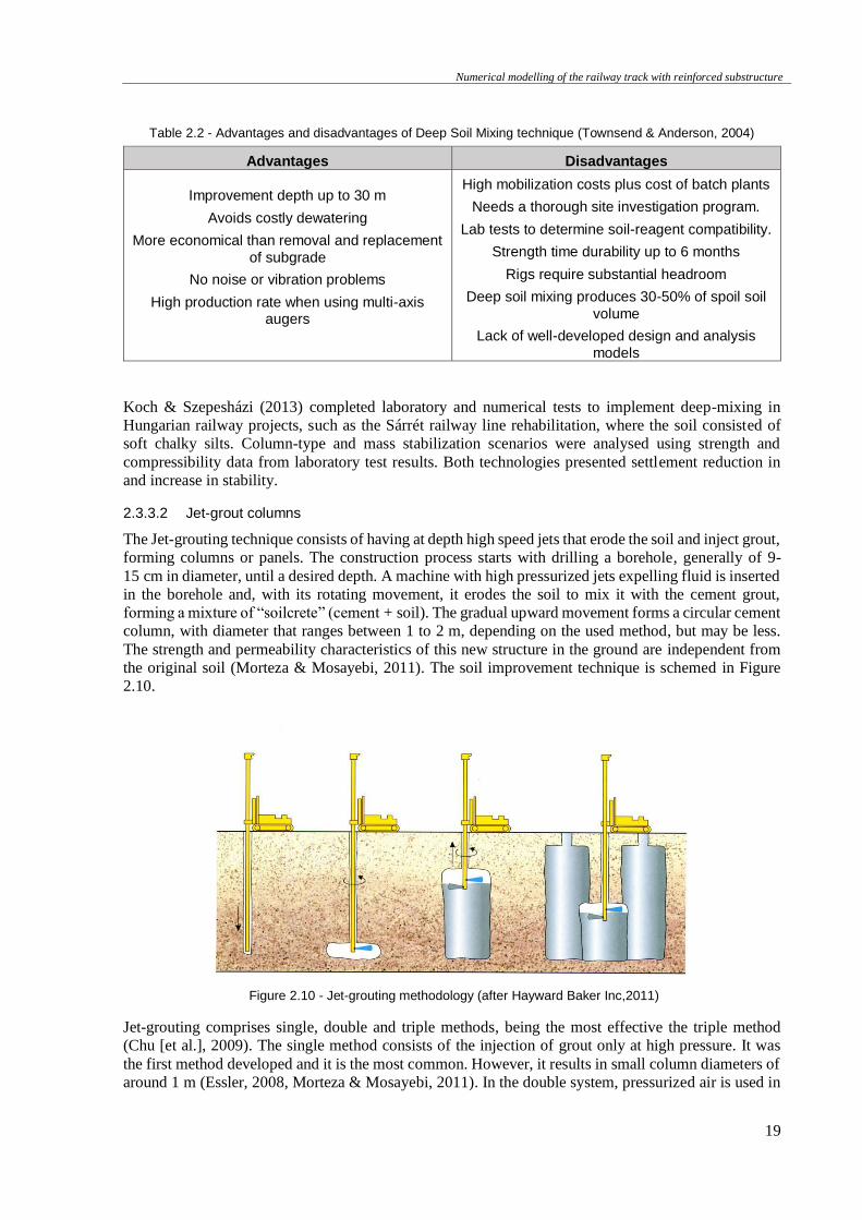
Numerical modelling of the railway track with reinforced substructure
19
Table 2.2 - Advantages and disadvantages of Deep Soil Mixing technique (Townsend & Anderson, 2004)
Advantages Disadvantages
Improvement depth up to 30 m
Avoids costly dewatering
More economical than removal and replacement
of subgrade
No noise or vibration problems
High production rate when using multi-axis augers
High mobilization costs plus cost of batch plants
Needs a thorough site investigation program.
Lab tests to determine soil-reagent compatibility.
Strength time durability up to 6 months
Rigs require substantial headroom
Deep soil mixing produces 30-50% of spoil soil
volume
Lack of well-developed design and analysis
models
Koch & Szepesházi (2013) completed laboratory and numerical tests to implement deep-mixing in
Hungarian railway projects, such as the Sárrét railway line rehabilitation, where the soil consisted of
soft chalky silts. Column-type and mass stabilization scenarios were analysed using strength and
compressibility data from laboratory test results. Both technologies presented settlement reduction in
and increase in stability.
2.3.3.2 Jet-grout columns
The Jet-grouting technique consists of having at depth high speed jets that erode the soil and inject grout,
forming columns or panels. The construction process starts with drilling a borehole, generally of 9-
15 cm in diameter, until a desired depth. A machine with high pressurized jets expelling fluid is inserted
in the borehole and, with its rotating movement, it erodes the soil to mix it with the cement grout,
forming a mixture of “soilcrete” (cement + soil). The gradual upward movement forms a circular cement
column, with diameter that ranges between 1 to 2 m, depending on the used method, but may be less.
The strength and permeability characteristics of this new structure in the ground are independent from
the original soil (Morteza & Mosayebi, 2011). The soil improvement technique is schemed in Figure
2.10.
Figure 2.10 - Jet-grouting methodology (after Hayward Baker Inc,2011)
Jet-grouting comprises single, double and triple methods, being the most effective the triple method
(Chu [et al.], 2009). The single method consists of the injection of grout only at high pressure. It was
the first method developed and it is the most common. However, it results in small column diameters of
around 1 m (Essler, 2008, Morteza & Mosayebi, 2011). In the double system, pressurized air is used in
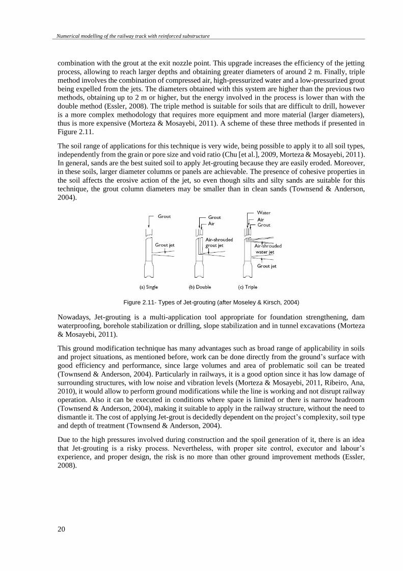
Numerical modelling of the railway track with reinforced substructure
20
combination with the grout at the exit nozzle point. This upgrade increases the efficiency of the jetting
process, allowing to reach larger depths and obtaining greater diameters of around 2 m. Finally, triple
method involves the combination of compressed air, high-pressurized water and a low-pressurized grout
being expelled from the jets. The diameters obtained with this system are higher than the previous two
methods, obtaining up to 2 m or higher, but the energy involved in the process is lower than with the
double method (Essler, 2008). The triple method is suitable for soils that are difficult to drill, however
is a more complex methodology that requires more equipment and more material (larger diameters),
thus is more expensive (Morteza & Mosayebi, 2011). A scheme of these three methods if presented in
Figure 2.11.
The soil range of applications for this technique is very wide, being possible to apply it to all soil types,
independently from the grain or pore size and void ratio (Chu [et al.], 2009, Morteza & Mosayebi, 2011).
In general, sands are the best suited soil to apply Jet-grouting because they are easily eroded. Moreover,
in these soils, larger diameter columns or panels are achievable. The presence of cohesive properties in
the soil affects the erosive action of the jet, so even though silts and silty sands are suitable for this
technique, the grout column diameters may be smaller than in clean sands (Townsend & Anderson,
2004).
Figure 2.11- Types of Jet-grouting (after Moseley & Kirsch, 2004)
Nowadays, Jet-grouting is a multi-application tool appropriate for foundation strengthening, dam
waterproofing, borehole stabilization or drilling, slope stabilization and in tunnel excavations (Morteza
& Mosayebi, 2011).
This ground modification technique has many advantages such as broad range of applicability in soils
and project situations, as mentioned before, work can be done directly from the ground’s surface with
good efficiency and performance, since large volumes and area of problematic soil can be treated
(Townsend & Anderson, 2004). Particularly in railways, it is a good option since it has low damage of
surrounding structures, with low noise and vibration levels (Morteza & Mosayebi, 2011, Ribeiro, Ana,
2010), it would allow to perform ground modifications while the line is working and not disrupt railway
operation. Also it can be executed in conditions where space is limited or there is narrow headroom
(Townsend & Anderson, 2004), making it suitable to apply in the railway structure, without the need to
dismantle it. The cost of applying Jet-grout is decidedly dependent on the project’s complexity, soil type
and depth of treatment (Townsend & Anderson, 2004).
Due to the high pressures involved during construction and the spoil generation of it, there is an idea
that Jet-grouting is a risky process. Nevertheless, with proper site control, executor and labour’s
experience, and proper design, the risk is no more than other ground improvement methods (Essler,
2008).

Numerical modelling of the railway track with reinforced substructure
21

Numerical modelling of the railway track with reinforced substructure
22
Numerical modelling of the railway track with reinforced substructure
23
PARAMETRIC NUMERICAL STUDIES
ON INTERFACES USING FLAC3D
3.1 GENERAL CONSIDERATIONS
One of the purposes of this thesis is to analyse the utility and performance of railway track subgrade
improvement solutions, resorting to Jet-grout columns, using a three-dimensional numerical model of a
railway track. However, due to the complexity of such numerical modelling, in terms of geometry, size
(number of elements, nodes and degrees of freedom), different mesh types/shapes, combination of
diverse materials and also due to the sleeper-ballast interaction behaviour, in some situations it may be
recommended to introduce interfaces or other numerical techniques in the model (Paixão & Fortunato,
2010, Wu [et al.], 2016). Therefore, one must first study, in a smaller scale, how two generic bodies,
with different soil layers and mesh type, interact using those numerical techniques to better understand
how to model them further on.
The focus of the parametric studies presented in this chapter was to see if there are differences in the
model behaviour, analysing stress and displacement fields, when we have different soil layers with
different mesh types, especially, cylindrical zones on the bottom layer combined with brick zones
(orthogonal grids) on top and their interaction.
3.2 NUMERICAL MODELLING OF THE RAILWAY TRACK STRUCTURAL BEHAVIOUR
Railway lines are rather complex structures with material and structural non-linear behaviour (Paixão &
Fortunato, 2009). When studying the track’s behaviour, one must consider the interaction between the
various components that make up this system in order to determine accurate strain and stress results due
to train loads.
Despite the existence of analytical methods that try to reproduce the effects of the train’s three-
dimensional loading (vertical, lateral and longitudinal), numerical methods such as the finite element
method (FEM) or the finite difference method (FDM) are generally more adequate to simulate train
loads and implement non-linear behaviour to the track’s various materials (Fortunato, 2005, Paixão &
Fortunato, 2009). Despite the train load being made up of three main components, as mentioned before,
track analysis studies have been focusing rather on the effects only due to vertical loading (Fortunato,
2005, Fortunato & Resende, 2006, Varandas [et al.], 2016).
With the increase of computational capacity, the implementation of such numerical methods has become
a common practice, allowing users to generate larger and more complex numerical models to achieve a
better understanding of the track system’s behaviour. A big advantage of implementing such numerical
approaches is that it allows to perform parametric studies, analysing the effect of variation of numerous
properties.
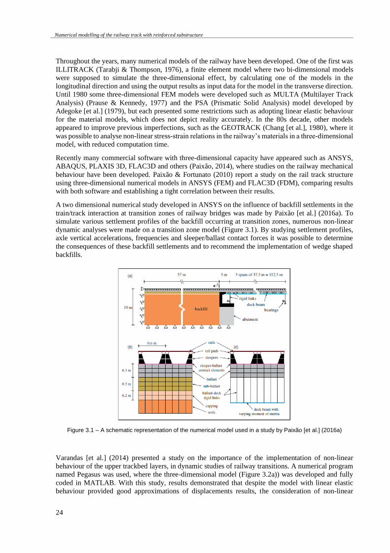
Numerical modelling of the railway track with reinforced substructure
24
Throughout the years, many numerical models of the railway have been developed. One of the first was
ILLITRACK (Tarabji & Thompson, 1976), a finite element model where two bi-dimensional models
were supposed to simulate the three-dimensional effect, by calculating one of the models in the
longitudinal direction and using the output results as input data for the model in the transverse direction.
Until 1980 some three-dimensional FEM models were developed such as MULTA (Multilayer Track
Analysis) (Prause & Kennedy, 1977) and the PSA (Prismatic Solid Analysis) model developed by
Adegoke [et al.] (1979), but each presented some restrictions such as adopting linear elastic behaviour
for the material models, which does not depict reality accurately. In the 80s decade, other models
appeared to improve previous imperfections, such as the GEOTRACK (Chang [et al.], 1980), where it
was possible to analyse non-linear stress-strain relations in the railway’s materials in a three-dimensional
model, with reduced computation time.
Recently many commercial software with three-dimensional capacity have appeared such as ANSYS,
ABAQUS, PLAXIS 3D, FLAC3D and others (Paixão, 2014), where studies on the railway mechanical
behaviour have been developed. Paixão & Fortunato (2010) report a study on the rail track structure
using three-dimensional numerical models in ANSYS (FEM) and FLAC3D (FDM), comparing results
with both software and establishing a tight correlation between their results.
A two dimensional numerical study developed in ANSYS on the influence of backfill settlements in the
train/track interaction at transition zones of railway bridges was made by Paixão [et al.] (2016a). To
simulate various settlement profiles of the backfill occurring at transition zones, numerous non-linear
dynamic analyses were made on a transition zone model (Figure 3.1). By studying settlement profiles,
axle vertical accelerations, frequencies and sleeper/ballast contact forces it was possible to determine
the consequences of these backfill settlements and to recommend the implementation of wedge shaped
backfills.
Figure 3.1 – A schematic representation of the numerical model used in a study by Paixão [et al.] (2016a)
Varandas [et al.] (2014) presented a study on the importance of the implementation of non-linear
behaviour of the upper trackbed layers, in dynamic studies of railway transitions. A numerical program
named Pegasus was used, where the three-dimensional model (Figure 3.2a)) was developed and fully
coded in MATLAB. With this study, results demonstrated that despite the model with linear elastic
behaviour provided good approximations of displacements results, the consideration of non-linear
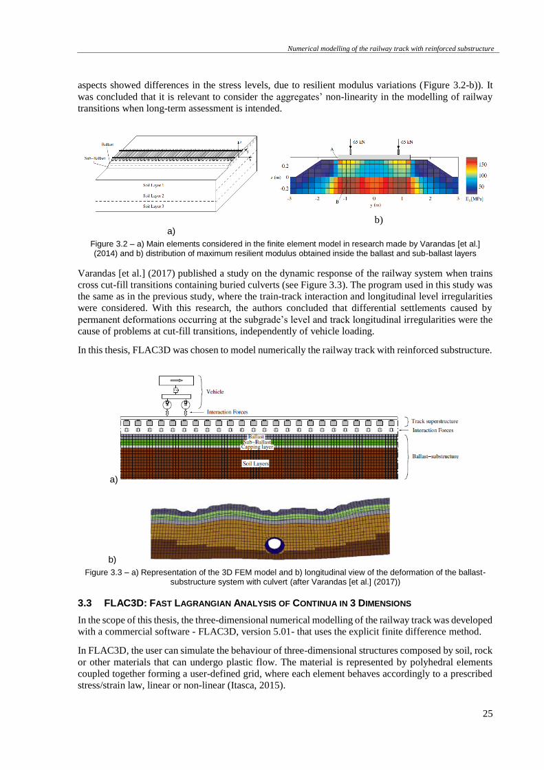
Numerical modelling of the railway track with reinforced substructure
25
aspects showed differences in the stress levels, due to resilient modulus variations (Figure 3.2-b)). It
was concluded that it is relevant to consider the aggregates’ non-linearity in the modelling of railway
transitions when long-term assessment is intended.
a)
b)
Figure 3.2 – a) Main elements considered in the finite element model in research made by Varandas [et al.] (2014) and b) distribution of maximum resilient modulus obtained inside the ballast and sub-ballast layers
Varandas [et al.] (2017) published a study on the dynamic response of the railway system when trains
cross cut-fill transitions containing buried culverts (see Figure 3.3). The program used in this study was
the same as in the previous study, where the train-track interaction and longitudinal level irregularities
were considered. With this research, the authors concluded that differential settlements caused by
permanent deformations occurring at the subgrade’s level and track longitudinal irregularities were the
cause of problems at cut-fill transitions, independently of vehicle loading.
In this thesis, FLAC3D was chosen to model numerically the railway track with reinforced substructure.
a)
b)
Figure 3.3 – a) Representation of the 3D FEM model and b) longitudinal view of the deformation of the ballast-substructure system with culvert (after Varandas [et al.] (2017))
3.3 FLAC3D: FAST LAGRANGIAN ANALYSIS OF CONTINUA IN 3 DIMENSIONS
In the scope of this thesis, the three-dimensional numerical modelling of the railway track was developed
with a commercial software - FLAC3D, version 5.01- that uses the explicit finite difference method.
In FLAC3D, the user can simulate the behaviour of three-dimensional structures composed by soil, rock
or other materials that can undergo plastic flow. The material is represented by polyhedral elements
coupled together forming a user-defined grid, where each element behaves accordingly to a prescribed
stress/strain law, linear or non-linear (Itasca, 2015).
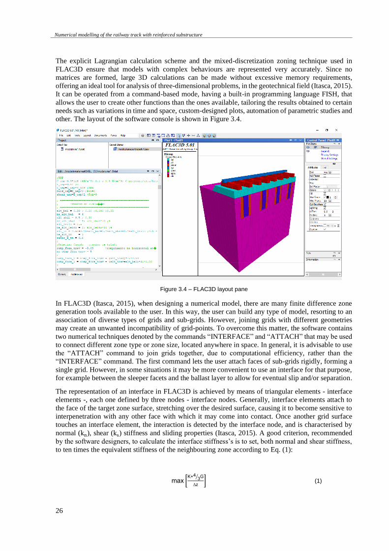
Numerical modelling of the railway track with reinforced substructure
26
The explicit Lagrangian calculation scheme and the mixed-discretization zoning technique used in
FLAC3D ensure that models with complex behaviours are represented very accurately. Since no
matrices are formed, large 3D calculations can be made without excessive memory requirements,
offering an ideal tool for analysis of three-dimensional problems, in the geotechnical field (Itasca, 2015).
It can be operated from a command-based mode, having a built-in programming language FISH, that
allows the user to create other functions than the ones available, tailoring the results obtained to certain
needs such as variations in time and space, custom-designed plots, automation of parametric studies and
other. The layout of the software console is shown in Figure 3.4.
Figure 3.4 – FLAC3D layout pane
In FLAC3D (Itasca, 2015), when designing a numerical model, there are many finite difference zone
generation tools available to the user. In this way, the user can build any type of model, resorting to an
association of diverse types of grids and sub-grids. However, joining grids with different geometries
may create an unwanted incompatibility of grid-points. To overcome this matter, the software contains
two numerical techniques denoted by the commands “INTERFACE” and “ATTACH” that may be used
to connect different zone type or zone size, located anywhere in space. In general, it is advisable to use
the “ATTACH” command to join grids together, due to computational efficiency, rather than the
“INTERFACE” command. The first command lets the user attach faces of sub-grids rigidly, forming a
single grid. However, in some situations it may be more convenient to use an interface for that purpose,
for example between the sleeper facets and the ballast layer to allow for eventual slip and/or separation.
The representation of an interface in FLAC3D is achieved by means of triangular elements - interface
elements -, each one defined by three nodes - interface nodes. Generally, interface elements attach to
the face of the target zone surface, stretching over the desired surface, causing it to become sensitive to
interpenetration with any other face with which it may come into contact. Once another grid surface
touches an interface element, the interaction is detected by the interface node, and is characterised by
normal (kn), shear (ks) stiffness and sliding properties (Itasca, 2015). A good criterion, recommended
by the software designers, to calculate the interface stiffness’s is to set, both normal and shear stiffness,
to ten times the equivalent stiffness of the neighbouring zone according to Eq. (1):
max [K+4
3⁄ G
∆z] (1)
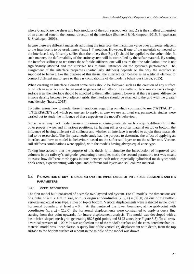
Numerical modelling of the railway track with reinforced substructure
27
where G and K are the shear and bulk modulus of the soil, respectively, and ∆z is the smallest dimension
of an attached zone in the normal direction of the interface (Esmaeili & Hakimpour, 2015, Pirapakaran
& Sivakugan, 2006).
In case there are different materials adjoining the interface, the maximum value over all zones adjacent
to the interface is to be used, hence “max [ ]” notation. However, if one of the materials connected to
the interface is significantly stiffer than the other, then Eq. (1) should be applied to the softer side. In
such manner, the deformability of the entire system will be controlled by the softer material. By setting
the interface stiffness to ten times the soft-side stiffness, one will ensure that the calculation time is not
significantly affected and the interface has minimal influence on the system’s performance. The
assignment of the interface properties (particularly stiffness) depends on the way the interface is
supposed to behave. For the purpose of this thesis, the interface can behave as an artificial element to
connect different mesh types so there is compatibility of the model’s behaviour (Itasca, 2015).
When creating an interface element some rules should be followed such as the creation of any surface
on which an interface is to be set must be generated initially or if a smaller surface area contacts a larger
surface area, the interface should be attached to the smaller region. However, if there is a great difference
in zone density between two adjacent grids, the interface should be attached to the grid with the greater
zone density (Itasca, 2015).
To better assess how to model these interactions, regarding on which command to use (“ATTACH” or
“INTERFACE”) and which parameters to apply, in case we use an interface, parametric studies were
carried out to study the influence of these aspects on the model’s behaviour.
Since the railway track model consists of various adjoining materials, each one quite different from the
other property wise, and in various positions, i.e. having stiffer or softer material on top or bottom, the
influence of having different soil stiffness and whether an interface is needed to adjoin these materials
had to be researched. The first parametric study had the purpose to determine the effect of applying an
interface and how to model its behaviour, based on the softer soil layer or on the stiffer one. Various
soil stiffness combinations were applied, with the models having always equal zone type.
Taking into account that the purpose of this thesis is to simulate the introduction of improved soil
columns in the railway’s subgrade, generating a complex mesh, the second parametric test was meant
to assess how different mesh types interact between each other, especially cylindrical mesh types with
brick zones, experimenting with equal and different soil layers and soil column material.
3.4 PARAMETRIC STUDY TO UNDERSTAND THE IMPORTANCE OF INTERFACE ELEMENTS AND ITS
PARAMETERS
3.4.1 MODEL DESCRIPTION
The first model built consisted of a simple two-layered soil system. For all models, the dimensions are
of a cube of 4 m x 4 m in size, with its origin at coordinates (x, y, z) = (0,0,0) on one of the bottom
vertexes and equal zone type, either on top or bottom. Vertical displacements were restricted in the lower
horizontal boundary, at level z = 0 m. At the centre of the lower boundary, at the grid-point with
coordinates (x, y, z) = (2,2,0), the horizontal displacements were constrained to apply a query line
starting from that point upwards, for future displacement analysis. The model was developed with a
basic brick-shaped mesh grid, generating 9826 grid-points and 8192 zones (see Figure 3.5). To all tests,
a vertical pressure of -100 MPa was applied on top of the model’s surface and the considered mechanical
material model was linear elastic. A query line of the vertical (z) displacement with depth, from the top
surface to the bottom surface of a point in the middle of the model was drawn.
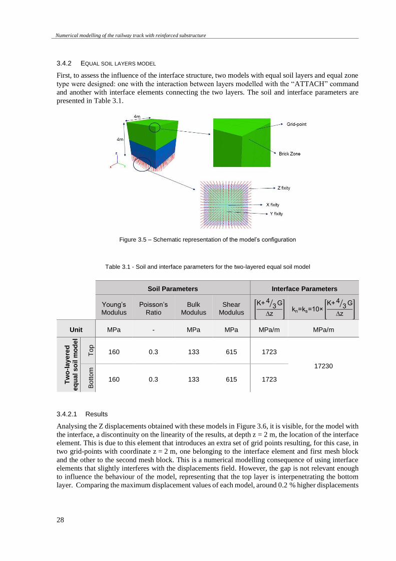
Numerical modelling of the railway track with reinforced substructure
28
3.4.2 EQUAL SOIL LAYERS MODEL
First, to assess the influence of the interface structure, two models with equal soil layers and equal zone
type were designed: one with the interaction between layers modelled with the “ATTACH” command
and another with interface elements connecting the two layers. The soil and interface parameters are
presented in Table 3.1.
Figure 3.5 – Schematic representation of the model’s configuration
Table 3.1 - Soil and interface parameters for the two-layered equal soil model
3.4.2.1 Results
Analysing the Z displacements obtained with these models in Figure 3.6, it is visible, for the model with
the interface, a discontinuity on the linearity of the results, at depth z = 2 m, the location of the interface
element. This is due to this element that introduces an extra set of grid points resulting, for this case, in
two grid-points with coordinate z = 2 m, one belonging to the interface element and first mesh block
and the other to the second mesh block. This is a numerical modelling consequence of using interface
elements that slightly interferes with the displacements field. However, the gap is not relevant enough
to influence the behaviour of the model, representing that the top layer is interpenetrating the bottom
layer. Comparing the maximum displacement values of each model, around 0.2 % higher displacements
Soil Parameters Interface Parameters
Young’s
Modulus
Poisson’s
Ratio
Bulk
Modulus
Shear
Modulus [K+ 4
3⁄ G
∆z] kn=ks=10× [
K+ 43⁄ G
∆z]
Unit MPa - MPa MPa MPa/m MPa/m
Tw
o-l
ay
ere
d
eq
ua
l s
oil
mo
de
l
To
p
160 0.3 133 615 1723
17230
Bo
tto
m
160 0.3 133 615 1723
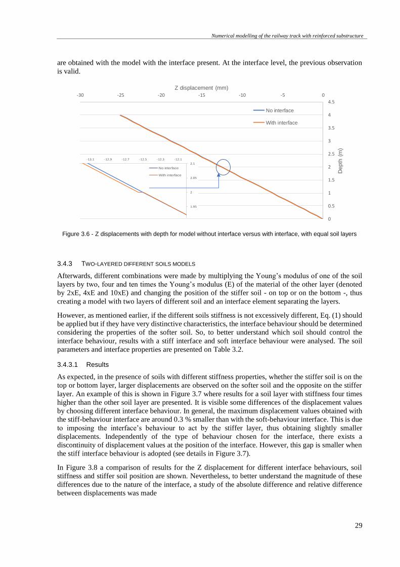
Numerical modelling of the railway track with reinforced substructure
29
are obtained with the model with the interface present. At the interface level, the previous observation
is valid.
Figure 3.6 - Z displacements with depth for model without interface versus with interface, with equal soil layers
3.4.3 TWO-LAYERED DIFFERENT SOILS MODELS
Afterwards, different combinations were made by multiplying the Young’s modulus of one of the soil
layers by two, four and ten times the Young’s modulus (E) of the material of the other layer (denoted
by 2xE, 4xE and 10xE) and changing the position of the stiffer soil - on top or on the bottom -, thus
creating a model with two layers of different soil and an interface element separating the layers.
However, as mentioned earlier, if the different soils stiffness is not excessively different, Eq. (1) should
be applied but if they have very distinctive characteristics, the interface behaviour should be determined
considering the properties of the softer soil. So, to better understand which soil should control the
interface behaviour, results with a stiff interface and soft interface behaviour were analysed. The soil
parameters and interface properties are presented on Table 3.2.
3.4.3.1 Results
As expected, in the presence of soils with different stiffness properties, whether the stiffer soil is on the
top or bottom layer, larger displacements are observed on the softer soil and the opposite on the stiffer
layer. An example of this is shown in Figure 3.7 where results for a soil layer with stiffness four times
higher than the other soil layer are presented. It is visible some differences of the displacement values
by choosing different interface behaviour. In general, the maximum displacement values obtained with
the stiff-behaviour interface are around 0.3 % smaller than with the soft-behaviour interface. This is due
to imposing the interface’s behaviour to act by the stiffer layer, thus obtaining slightly smaller
displacements. Independently of the type of behaviour chosen for the interface, there exists a
discontinuity of displacement values at the position of the interface. However, this gap is smaller when
the stiff interface behaviour is adopted (see details in Figure 3.7).
In Figure 3.8 a comparison of results for the Z displacement for different interface behaviours, soil
stiffness and stiffer soil position are shown. Nevertheless, to better understand the magnitude of these
differences due to the nature of the interface, a study of the absolute difference and relative difference
between displacements was made
0
0.5
1
1.5
2
2.5
3
3.5
4
4.5
-30 -25 -20 -15 -10 -5 0
Depth
(m
)
Z displacement (mm)
No interface
With interface
1.9
1.95
2
2.05
2.1
-13.5 -13.3 -13.1 -12.9 -12.7 -12.5 -12.3 -12.1
No interface
With interface
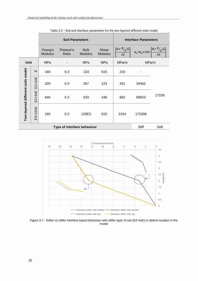
Numerical modelling of the railway track with reinforced substructure
30
Table 3.2 - Soil and interface parameters for the two-layered different soils model
Figure 3.7 - Softer vs stiffer interface based behaviour with stiffer layer of soil (E2=4xE) in distinct location in the model
0
0.5
1
1.5
2
2.5
3
3.5
4
4.5
-20 -18 -16 -14 -12 -10 -8 -6 -4 -2 0
De
pth
(m
)
Z displacement (mm)
Interface softer 4xE bottom Interface stiffer 4xE bottom
Interface softer 4xE top Interface stiffer 4xE top
1.8
1.85
1.9
1.95
2
2.05
2.1
2.15
2.2
-5 -4.5 -4 -3.5 -3 -2.5 -2
De
pth
(m)
Z displacement (mm)
1.7
1.8
1.9
2
2.1
2.2
2.3
-13 -12.9 -12.8 -12.7 -12.6 -12.5 -12.4 -12.3 -12.2 -12.1 -12
De
pth
(m
)
Z displacement (mm)
Soil Parameters Interface Parameters
Young’s
Modulus
Poisson’s
Ratio
Bulk
Modulus
Shear
Modulus [K+ 4
3⁄ G
∆z] kn=ks=10× [
K+ 43⁄ G
∆z]
Unit MPa - MPa MPa MPa/m MPa/m
Tw
o-l
ay
ere
d d
iffe
ren
t s
oils
mo
de
l
E
160 0.3 133 615 215 -
17230
E1
=2
xE
320 0.3 267 123 431 34462
E2
=4
xE
640 0.3 533 246 862 68923
E3
=1
0xE
160 0.3 133E3 615 2154 172308
Type of interface behaviour Stiff Soft
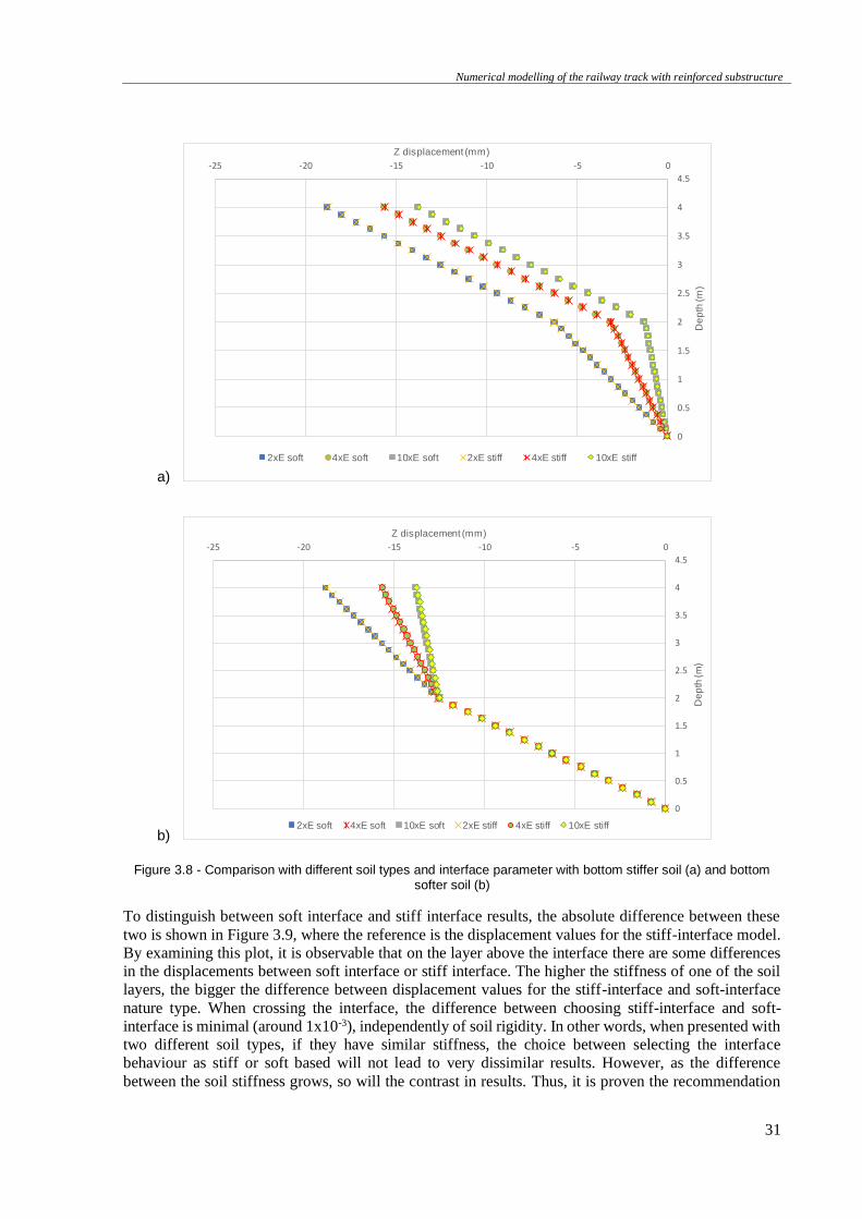
Numerical modelling of the railway track with reinforced substructure
31
a)
b)
Figure 3.8 - Comparison with different soil types and interface parameter with bottom stiffer soil (a) and bottom softer soil (b)
To distinguish between soft interface and stiff interface results, the absolute difference between these
two is shown in Figure 3.9, where the reference is the displacement values for the stiff-interface model.
By examining this plot, it is observable that on the layer above the interface there are some differences
in the displacements between soft interface or stiff interface. The higher the stiffness of one of the soil
layers, the bigger the difference between displacement values for the stiff-interface and soft-interface
nature type. When crossing the interface, the difference between choosing stiff-interface and soft-
interface is minimal (around 1x10⁻³), independently of soil rigidity. In other words, when presented with
two different soil types, if they have similar stiffness, the choice between selecting the interface
behaviour as stiff or soft based will not lead to very dissimilar results. However, as the difference
between the soil stiffness grows, so will the contrast in results. Thus, it is proven the recommendation
0
0.5
1
1.5
2
2.5
3
3.5
4
4.5
-25 -20 -15 -10 -5 0
De
pth
(m
)
Z displacement (mm)
2xE soft 4xE soft 10xE soft 2xE stiff 4xE stiff 10xE stiff
0
0.5
1
1.5
2
2.5
3
3.5
4
4.5
-25 -20 -15 -10 -5 0
De
pth
(m)
Z displacement (mm)
2xE soft 4xE soft 10xE soft 2xE stiff 4xE stiff 10xE stiff
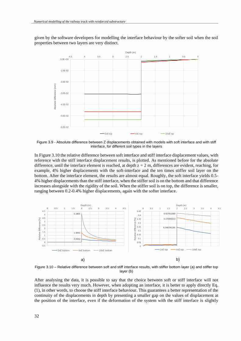
Numerical modelling of the railway track with reinforced substructure
32
given by the software developers for modelling the interface behaviour by the softer soil when the soil
properties between two layers are very distinct.
Figure 3.9 - Absolute difference between Z displacements obtained with models with soft interface and with stiff interface, for different soil types in the layers
In Figure 3.10 the relative difference between soft interface and stiff interface displacement values, with
reference with the stiff interface displacement results, is plotted. As mentioned before for the absolute
difference, until the interface element is reached, at depth z = 2 m, differences are evident, reaching, for
example, 4% higher displacements with the soft-interface and the ten times stiffer soil layer on the
bottom. After the interface element, the results are almost equal. Roughly, the soft interface yields 0.5-
4% higher displacements than the stiff interface, when the stiffer soil is on the bottom and that difference
increases alongside with the rigidity of the soil. When the stiffer soil is on top, the difference is smaller,
ranging between 0.2-0.4% higher displacements, again with the softer interface.
a)
b)
Figure 3.10 – Relative difference between soft and stiff interface results, with stiffer bottom layer (a) and stiffer top layer (b)
After analysing the data, it is possible to say that the choice between soft or stiff interface will not
influence the results very much. However, when adopting an interface, it is better to apply directly Eq.
(1), in other words, to choose the stiff interface behaviour. This guarantees a better representation of the
continuity of the displacements in depth by presenting a smaller gap on the values of displacement at
the position of the interface, even if the deformation of the system with the stiff interface is slightly
-6.0E-02
-5.0E-02
-4.0E-02
-3.0E-02
-2.0E-02
-1.0E-02
0.0E+00
00.511.522.533.544.5A
bsolu
te d
iffere
nce (
mm
)Depth (m)
2xE top 4xE top 10xE top
0.4662
1.3845
4.1803
-0.5
0
0.5
1
1.5
2
2.5
3
3.5
4
4.5
0 0.5 1 1.5 2 2.5 3 3.5 4 4.5
Re
lative
diffe
ren
ce
(%
)
Depth (m)
2xE bottom 4xE bottom 10xE bottom
0.246736136
0.370900313
0.427952069
0
0.05
0.1
0.15
0.2
0.25
0.3
0.35
0.4
0.45
0 0.5 1 1.5 2 2.5 3 3.5 4 4.5
Re
lative
diffe
ren
ce
(%
)
Depth (m)
2xE top 4xE top 10xE top
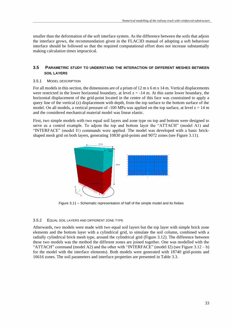
Numerical modelling of the railway track with reinforced substructure
33
smaller than the deformation of the soft interface system. As the difference between the soils that adjoin
the interface grows, the recommendation given in the FLAC3D manual of adopting a soft behaviour
interface should be followed so that the required computational effort does not increase substantially
making calculation times impractical.
3.5 PARAMETRIC STUDY TO UNDERSTAND THE INTERACTION OF DIFFERENT MESHES BETWEEN
SOIL LAYERS
3.5.1 MODEL DESCRIPTION
For all models in this section, the dimensions are of a prism of 12 m x 6 m x 14 m. Vertical displacements
were restricted in the lower horizontal boundary, at level z = -14 m. At this same lower boundary, the
horizontal displacement of the grid-point located in the centre of this face was constrained to apply a
query line of the vertical (z) displacement with depth, from the top surface to the bottom surface of the
model. On all models, a vertical pressure of -100 MPa was applied on the top surface, at level z = 14 m
and the considered mechanical material model was linear elastic.
First, two simple models with two equal soil layers and zone type on top and bottom were designed to
serve as a control example. To adjoin the top and bottom layer the “ATTACH” (model A1) and
“INTERFACE” (model I1) commands were applied. The model was developed with a basic brick-
shaped mesh grid on both layers, generating 10830 grid-points and 9072 zones (see Figure 3.11).
Figure 3.11 – Schematic representation of half of the simple model and its fixities
3.5.2 EQUAL SOIL LAYERS AND DIFFERENT ZONE TYPE
Afterwards, two models were made with two equal soil layers but the top layer with simple brick zone
elements and the bottom layer with a cylindrical grid, to simulate the soil column, combined with a
radially cylindrical brick mesh type, around the cylindrical grid (Figure 3.12). The difference between
these two models was the method the different zones are joined together. One was modelled with the
“ATTACH” command (model A2) and the other with “INTERFACE” (model I2) (see Figure 3.12 – b)
for the model with the interface elements). Both models were generated with 18740 grid-points and
16616 zones. The soil parameters and interface properties are presented in Table 3.3.
6 m
14 m
12 m
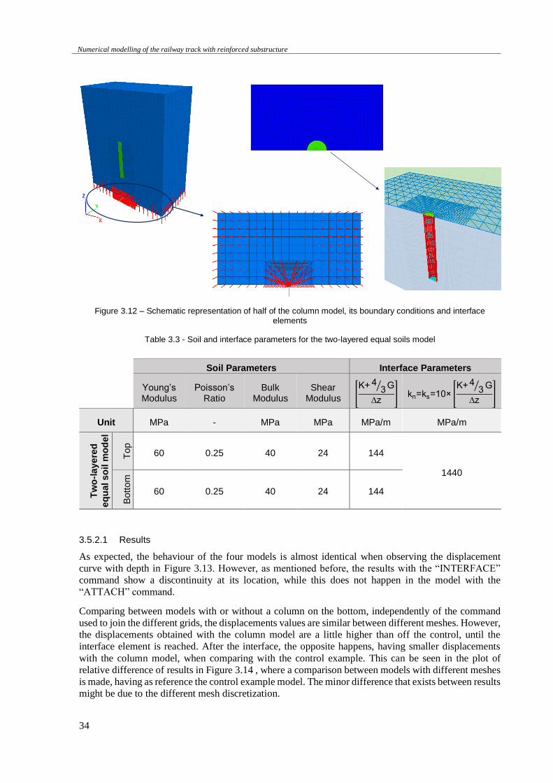
Numerical modelling of the railway track with reinforced substructure
34
Figure 3.12 – Schematic representation of half of the column model, its boundary conditions and interface elements
Table 3.3 - Soil and interface parameters for the two-layered equal soils model
3.5.2.1 Results
As expected, the behaviour of the four models is almost identical when observing the displacement
curve with depth in Figure 3.13. However, as mentioned before, the results with the “INTERFACE”
command show a discontinuity at its location, while this does not happen in the model with the
“ATTACH” command.
Comparing between models with or without a column on the bottom, independently of the command
used to join the different grids, the displacements values are similar between different meshes. However,
the displacements obtained with the column model are a little higher than off the control, until the
interface element is reached. After the interface, the opposite happens, having smaller displacements
with the column model, when comparing with the control example. This can be seen in the plot of
relative difference of results in Figure 3.14 , where a comparison between models with different meshes
is made, having as reference the control example model. The minor difference that exists between results
might be due to the different mesh discretization.
Soil Parameters Interface Parameters
Young’s Modulus
Poisson’s Ratio
Bulk Modulus
Shear Modulus
[K+ 4
3⁄ G
∆z] kn=ks=10× [
K+ 43⁄ G
∆z]
Unit MPa - MPa MPa MPa/m MPa/m
Tw
o-l
ay
ere
d
eq
ua
l s
oil
mo
de
l
To
p
60 0.25 40 24 144
1440
Bo
tto
m
60 0.25 40 24 144
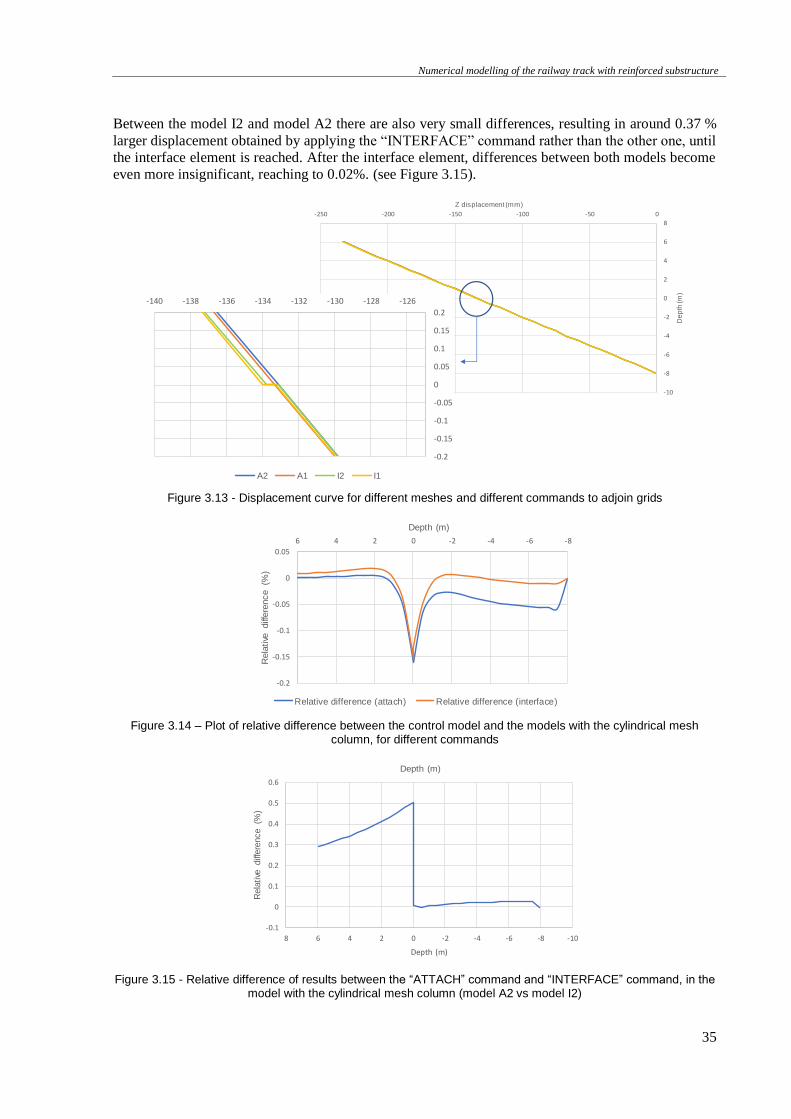
Numerical modelling of the railway track with reinforced substructure
35
Between the model I2 and model A2 there are also very small differences, resulting in around 0.37 %
larger displacement obtained by applying the “INTERFACE” command rather than the other one, until
the interface element is reached. After the interface element, differences between both models become
even more insignificant, reaching to 0.02%. (see Figure 3.15).
Figure 3.13 - Displacement curve for different meshes and different commands to adjoin grids
Figure 3.14 – Plot of relative difference between the control model and the models with the cylindrical mesh column, for different commands
Figure 3.15 - Relative difference of results between the “ATTACH” command and “INTERFACE” command, in the model with the cylindrical mesh column (model A2 vs model I2)
-10
-8
-6
-4
-2
0
2
4
6
8
-250 -200 -150 -100 -50 0
De
pth
(m
)
Z displacement (mm)
mesh with column (attach) No column (attach)
mesh with column (interface) No column (interface)
-0.2
-0.15
-0.1
-0.05
0
0.05
0.1
0.15
0.2
-140 -138 -136 -134 -132 -130 -128 -126
De
pth
(m
)
Z displacement (mm)
A2 A1 I2 I1
-0.2
-0.15
-0.1
-0.05
0
0.05
-8-6-4-20246
Rela
tive
diff
ere
nce (%
)
Depth (m)
Relative difference (attach) Relative difference (interface)
-0.2
-0.15
-0.1
-0.05
0
0.05
-8-6-4-20246
Rela
tive
diff
ere
nce (%
)
Depth (m)
Relative difference (attach) Relative difference (interface)-0.1
0
0.1
0.2
0.3
0.4
0.5
0.6
-10-8-6-4-202468
Rel
ati
ve D
iffe
ren
ce
Depth (m)

Numerical modelling of the railway track with reinforced substructure
36
3.5.3 DIFFERENT SOIL LAYERS AND ZONE TYPE
After the previous tests, where the interface elements acted only as a means to connect different mesh
types, one must study how this interface acts when in presence of different soil layers and mesh types,
on top and at the bottom, and its effect.
3.5.3.1 Different soil layers (column included in bottom layer)
Four models with the geometric properties of the previous ones were created, however, with different
soil properties on top and at the bottom. Two of them were made with regular mesh types on both layers,
one having the “ATTACH” command and other the “INTERFACE” command separating the soils
(models A1 and I1) (see Figure 3.16). The other two models had the mixed mesh type, also one with the
“ATTACH” and another with the “INTERFACE” separating the layers (model A2 and model I2) as
shown in Figure 3.17. The interface properties were based in the stiffer soil and the ground and interface
attributes are presented in Table 3.4.
a) b)
Figure 3.16 - Different soil layers with regular mesh models: a) “attach” command (model A1); b) “interface” command (model I1)
a) b)
Figure 3.17 - Different soil layers with mixed mesh models: a) “attach” command (model A2); b) “interface” command (model I2)
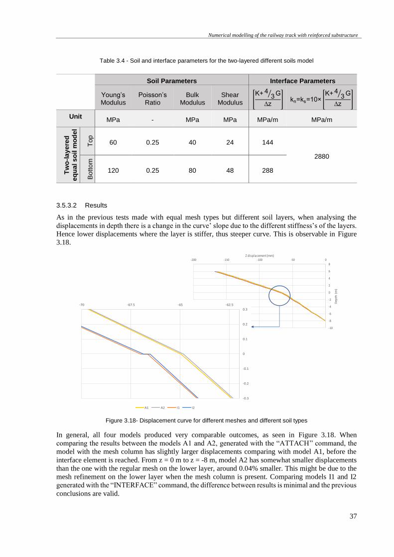
Numerical modelling of the railway track with reinforced substructure
37
Table 3.4 - Soil and interface parameters for the two-layered different soils model
3.5.3.2 Results
As in the previous tests made with equal mesh types but different soil layers, when analysing the
displacements in depth there is a change in the curve’ slope due to the different stiffness’s of the layers.
Hence lower displacements where the layer is stiffer, thus steeper curve. This is observable in Figure
3.18.
Figure 3.18- Displacement curve for different meshes and different soil types
In general, all four models produced very comparable outcomes, as seen in Figure 3.18. When
comparing the results between the models A1 and A2, generated with the “ATTACH” command, the
model with the mesh column has slightly larger displacements comparing with model A1, before the
interface element is reached. From z = 0 m to z = -8 m, model A2 has somewhat smaller displacements
than the one with the regular mesh on the lower layer, around 0.04% smaller. This might be due to the
mesh refinement on the lower layer when the mesh column is present. Comparing models I1 and I2
generated with the “INTERFACE” command, the difference between results is minimal and the previous
conclusions are valid.
-10
-8
-6
-4
-2
0
2
4
6
8
-200 -150 -100 -50 0
De
pth
(m
)
Z displacement (mm)
-0.3
-0.2
-0.1
0
0.1
0.2
0.3
-70 -67.5 -65 -62.5
A1 A2 I1 I2
Soil Parameters Interface Parameters
Young’s Modulus
Poisson’s Ratio
Bulk Modulus
Shear Modulus
[K+ 4
3⁄ G
∆z] kn=ks=10× [
K+ 43⁄ G
∆z]
Unit MPa - MPa MPa MPa/m MPa/m
Tw
o-l
ay
ere
d
eq
ua
l s
oil
mo
de
l
To
p
60 0.25 40 24 144
2880
Bo
tto
m
120 0.25 80 48 288
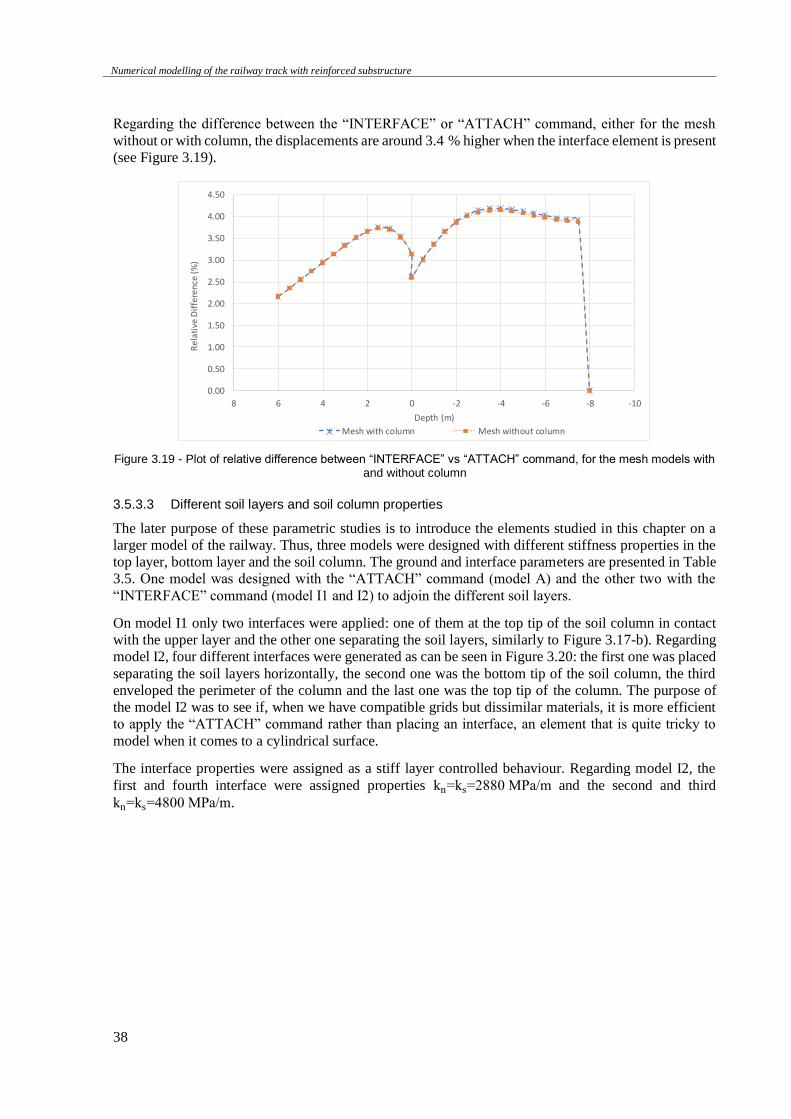
Numerical modelling of the railway track with reinforced substructure
38
Regarding the difference between the “INTERFACE” or “ATTACH” command, either for the mesh
without or with column, the displacements are around 3.4 % higher when the interface element is present
(see Figure 3.19).
Figure 3.19 - Plot of relative difference between “INTERFACE” vs “ATTACH” command, for the mesh models with and without column
3.5.3.3 Different soil layers and soil column properties
The later purpose of these parametric studies is to introduce the elements studied in this chapter on a
larger model of the railway. Thus, three models were designed with different stiffness properties in the
top layer, bottom layer and the soil column. The ground and interface parameters are presented in Table
3.5. One model was designed with the “ATTACH” command (model A) and the other two with the
“INTERFACE” command (model I1 and I2) to adjoin the different soil layers.
On model I1 only two interfaces were applied: one of them at the top tip of the soil column in contact
with the upper layer and the other one separating the soil layers, similarly to Figure 3.17-b). Regarding
model I2, four different interfaces were generated as can be seen in Figure 3.20: the first one was placed
separating the soil layers horizontally, the second one was the bottom tip of the soil column, the third
enveloped the perimeter of the column and the last one was the top tip of the column. The purpose of
the model I2 was to see if, when we have compatible grids but dissimilar materials, it is more efficient
to apply the “ATTACH” command rather than placing an interface, an element that is quite tricky to
model when it comes to a cylindrical surface.
The interface properties were assigned as a stiff layer controlled behaviour. Regarding model I2, the
first and fourth interface were assigned properties kn=ks=2880 MPa/m and the second and third
kn=ks=4800 MPa/m.
0.00
0.50
1.00
1.50
2.00
2.50
3.00
3.50
4.00
4.50
-10-8-6-4-202468
Re
lati
ve D
iffe
ren
ce (%
)
Depth (m)
Mesh with column Mesh without column
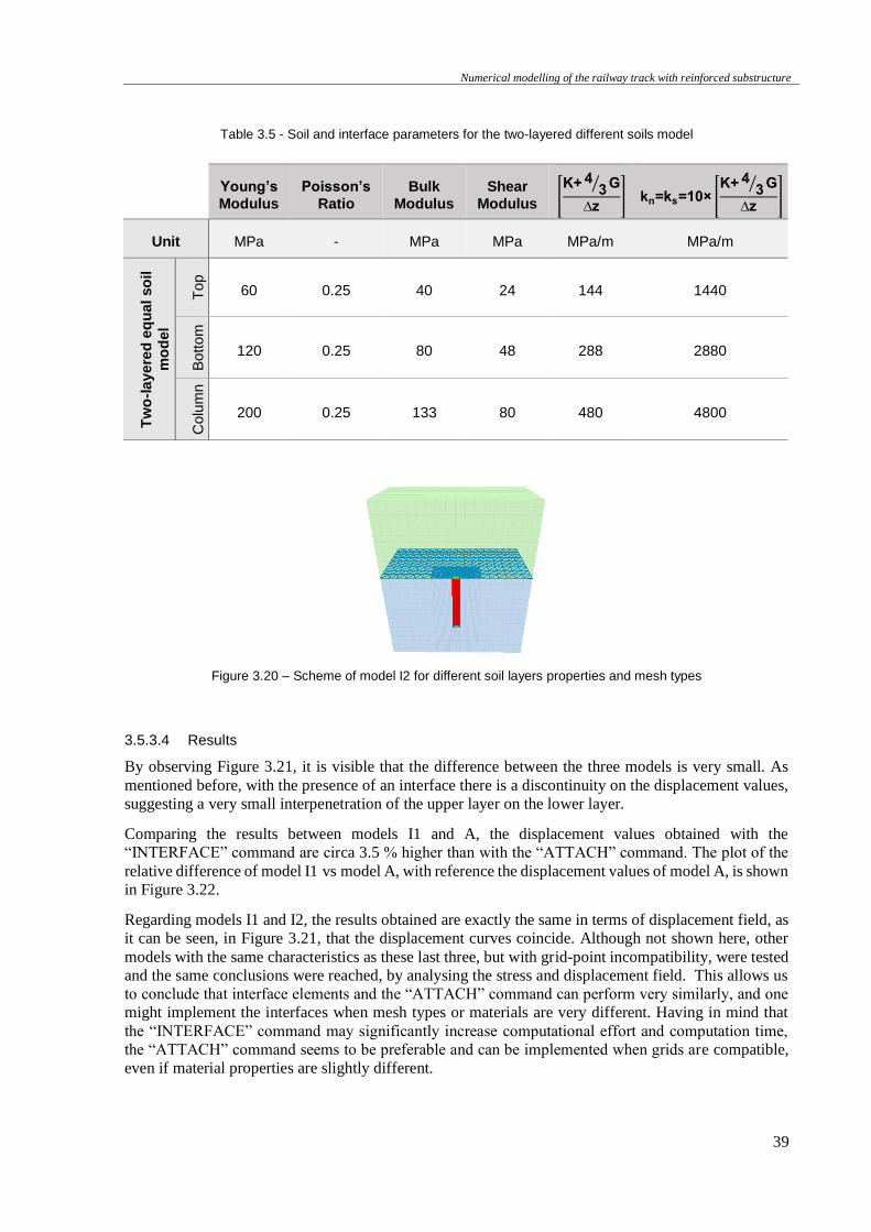
Numerical modelling of the railway track with reinforced substructure
39
Table 3.5 - Soil and interface parameters for the two-layered different soils model
Figure 3.20 – Scheme of model I2 for different soil layers properties and mesh types
3.5.3.4 Results
By observing Figure 3.21, it is visible that the difference between the three models is very small. As
mentioned before, with the presence of an interface there is a discontinuity on the displacement values,
suggesting a very small interpenetration of the upper layer on the lower layer.
Comparing the results between models I1 and A, the displacement values obtained with the
“INTERFACE” command are circa 3.5 % higher than with the “ATTACH” command. The plot of the
relative difference of model I1 vs model A, with reference the displacement values of model A, is shown
in Figure 3.22.
Regarding models I1 and I2, the results obtained are exactly the same in terms of displacement field, as
it can be seen, in Figure 3.21, that the displacement curves coincide. Although not shown here, other
models with the same characteristics as these last three, but with grid-point incompatibility, were tested
and the same conclusions were reached, by analysing the stress and displacement field. This allows us
to conclude that interface elements and the “ATTACH” command can perform very similarly, and one
might implement the interfaces when mesh types or materials are very different. Having in mind that
the “INTERFACE” command may significantly increase computational effort and computation time,
the “ATTACH” command seems to be preferable and can be implemented when grids are compatible,
even if material properties are slightly different.
Young’s
Modulus
Poisson’s
Ratio
Bulk
Modulus
Shear
Modulus [K+ 4
3⁄ G
∆z] kn=ks=10× [
K+ 43⁄ G
∆z]
Unit MPa - MPa MPa MPa/m MPa/m
Tw
o-l
ay
ere
d e
qu
al
so
il
mo
de
l
To
p
60 0.25 40 24 144 1440
Bo
tto
m
120 0.25 80 48 288 2880
Colu
mn
200 0.25 133 80 480 4800
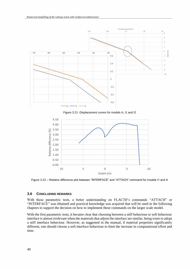
Numerical modelling of the railway track with reinforced substructure
40
Figure 3.21 -Displacement curves for models A, I1 and I2
Figure 3.22 – Relative difference plot between “INTERFACE” and “ATTACH” command for models I1 and A
3.6 CONCLUDING REMARKS
With these parametric tests, a better understanding on FLAC3D’s commands “ATTACH” or
“INTERFACE” was obtained and practical knowledge was acquired that will be used in the following
chapters to support the decision on how to implement these commands on the larger scale model.
With the first parametric tests, it became clear that choosing between a stiff behaviour or soft behaviour
interface is almost irrelevant when the materials that adjoin the interface are similar, being wiser to adopt
a stiff interface behaviour. However, as suggested in the manual, if material properties significantly
different, one should choose a soft interface behaviour to limit the increase in computational effort and
time.
-10
-8
-6
-4
-2
0
2
4
6
8
-170 -120 -70 -20 30
Dep
th (
m)
Z displacement (mm)
-0.6
-0.4
-0.2
0
0.2
0.4
0.6
-70 -68 -66 -64 -62 -60
A I1 I2
0.00
0.50
1.00
1.50
2.00
2.50
3.00
3.50
4.00
4.50
-10-50510
Rel
ativ
e di
ffer
ence
(%
)
Depth (m)
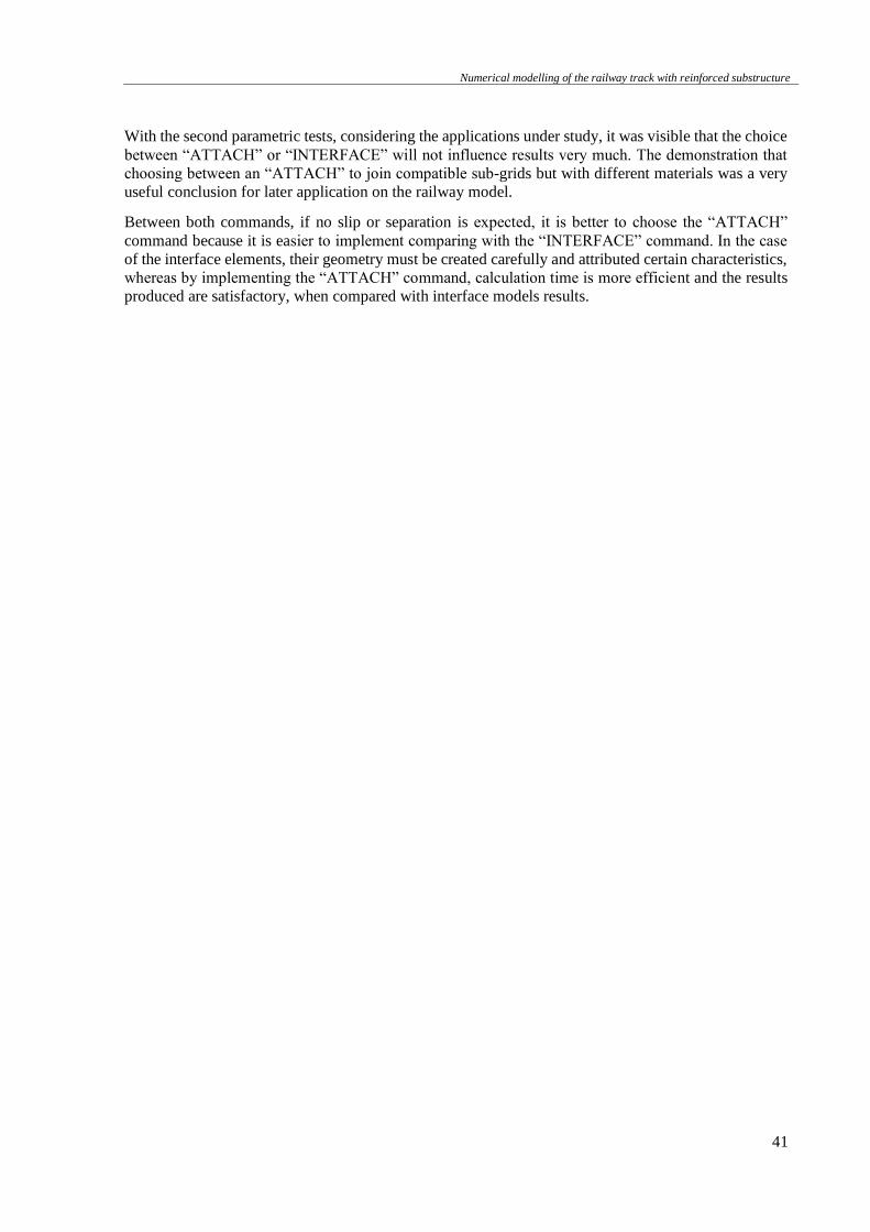
Numerical modelling of the railway track with reinforced substructure
41
With the second parametric tests, considering the applications under study, it was visible that the choice
between “ATTACH” or “INTERFACE” will not influence results very much. The demonstration that
choosing between an “ATTACH” to join compatible sub-grids but with different materials was a very
useful conclusion for later application on the railway model.
Between both commands, if no slip or separation is expected, it is better to choose the “ATTACH”
command because it is easier to implement comparing with the “INTERFACE” command. In the case
of the interface elements, their geometry must be created carefully and attributed certain characteristics,
whereas by implementing the “ATTACH” command, calculation time is more efficient and the results
produced are satisfactory, when compared with interface models results.

Numerical modelling of the railway track with reinforced substructure
42
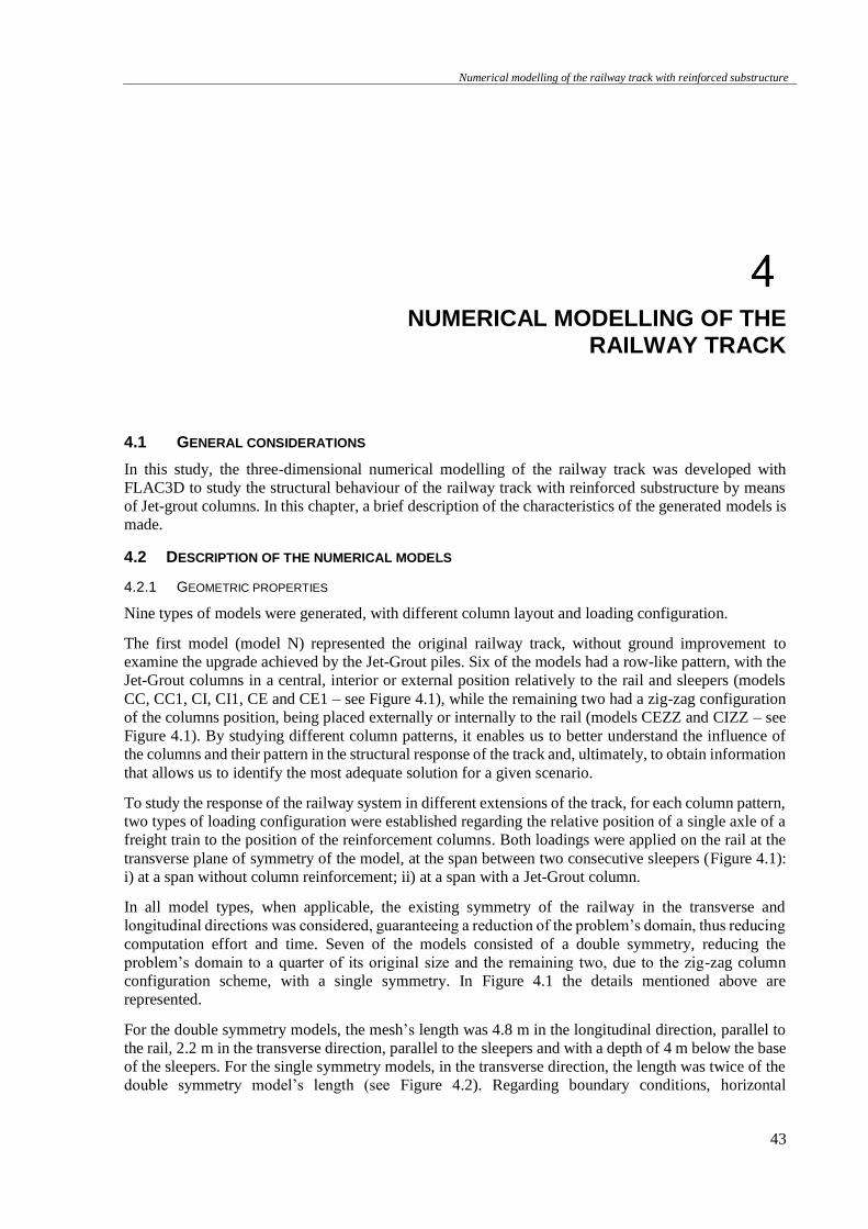
Numerical modelling of the railway track with reinforced substructure
43
NUMERICAL MODELLING OF THE
RAILWAY TRACK
4.1 GENERAL CONSIDERATIONS
In this study, the three-dimensional numerical modelling of the railway track was developed with
FLAC3D to study the structural behaviour of the railway track with reinforced substructure by means
of Jet-grout columns. In this chapter, a brief description of the characteristics of the generated models is
made.
4.2 DESCRIPTION OF THE NUMERICAL MODELS
4.2.1 GEOMETRIC PROPERTIES
Nine types of models were generated, with different column layout and loading configuration.
The first model (model N) represented the original railway track, without ground improvement to
examine the upgrade achieved by the Jet-Grout piles. Six of the models had a row-like pattern, with the
Jet-Grout columns in a central, interior or external position relatively to the rail and sleepers (models
CC, CC1, CI, CI1, CE and CE1 – see Figure 4.1), while the remaining two had a zig-zag configuration
of the columns position, being placed externally or internally to the rail (models CEZZ and CIZZ – see
Figure 4.1). By studying different column patterns, it enables us to better understand the influence of
the columns and their pattern in the structural response of the track and, ultimately, to obtain information
that allows us to identify the most adequate solution for a given scenario.
To study the response of the railway system in different extensions of the track, for each column pattern,
two types of loading configuration were established regarding the relative position of a single axle of a
freight train to the position of the reinforcement columns. Both loadings were applied on the rail at the
transverse plane of symmetry of the model, at the span between two consecutive sleepers (Figure 4.1):
i) at a span without column reinforcement; ii) at a span with a Jet-Grout column.
In all model types, when applicable, the existing symmetry of the railway in the transverse and
longitudinal directions was considered, guaranteeing a reduction of the problem’s domain, thus reducing
computation effort and time. Seven of the models consisted of a double symmetry, reducing the
problem’s domain to a quarter of its original size and the remaining two, due to the zig-zag column
configuration scheme, with a single symmetry. In Figure 4.1 the details mentioned above are
represented.
For the double symmetry models, the mesh’s length was 4.8 m in the longitudinal direction, parallel to
the rail, 2.2 m in the transverse direction, parallel to the sleepers and with a depth of 4 m below the base
of the sleepers. For the single symmetry models, in the transverse direction, the length was twice of the
double symmetry model’s length (see Figure 4.2). Regarding boundary conditions, horizontal
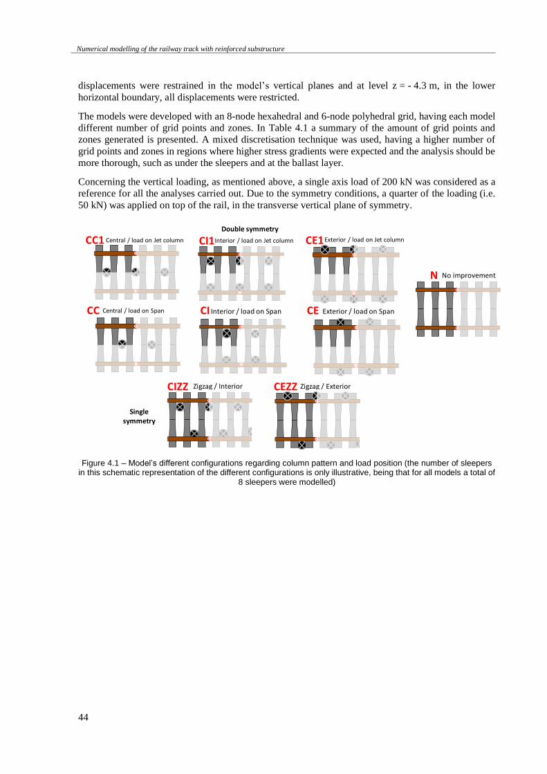
Numerical modelling of the railway track with reinforced substructure
44
displacements were restrained in the model’s vertical planes and at level z = - 4.3 m, in the lower
horizontal boundary, all displacements were restricted.
The models were developed with an 8-node hexahedral and 6-node polyhedral grid, having each model
different number of grid points and zones. In Table 4.1 a summary of the amount of grid points and
zones generated is presented. A mixed discretisation technique was used, having a higher number of
grid points and zones in regions where higher stress gradients were expected and the analysis should be
more thorough, such as under the sleepers and at the ballast layer.
Concerning the vertical loading, as mentioned above, a single axis load of 200 kN was considered as a
reference for all the analyses carried out. Due to the symmetry conditions, a quarter of the loading (i.e.
50 kN) was applied on top of the rail, in the transverse vertical plane of symmetry.
Figure 4.1 – Model’s different configurations regarding column pattern and load position (the number of sleepers in this schematic representation of the different configurations is only illustrative, being that for all models a total of
8 sleepers were modelled)
Double symmetry
Singlesymmetry
CC1
CC
CI1
CI
CE1
CE
CIZZ CEZZ
Central / load on Jet column Interior / load on Jet column Exterior / load on Jet column
Central / load on Span Interior / load on Span Exterior / load on Span
Zigzag / Interior Zigzag / Exterior
N No improvement
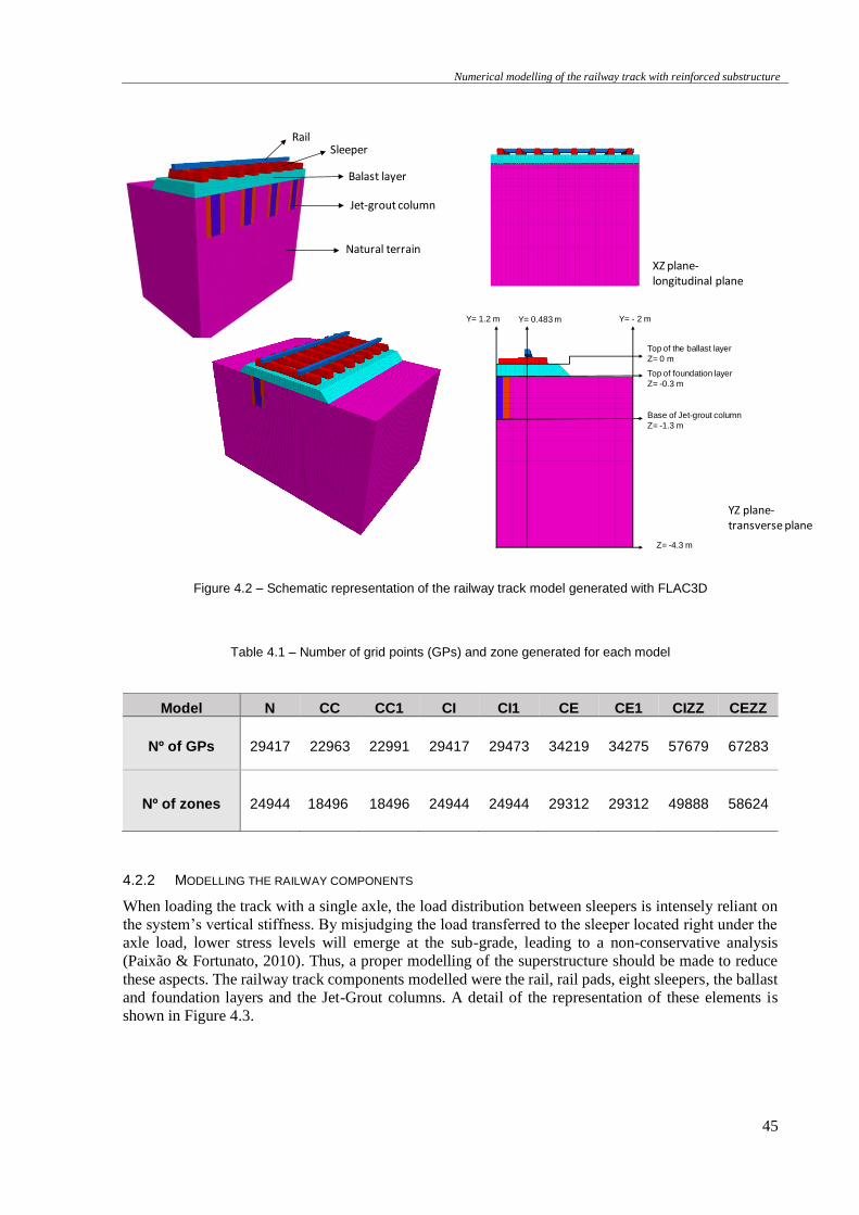
Numerical modelling of the railway track with reinforced substructure
45
Figure 4.2 – Schematic representation of the railway track model generated with FLAC3D
Table 4.1 – Number of grid points (GPs) and zone generated for each model
4.2.2 MODELLING THE RAILWAY COMPONENTS
When loading the track with a single axle, the load distribution between sleepers is intensely reliant on
the system’s vertical stiffness. By misjudging the load transferred to the sleeper located right under the
axle load, lower stress levels will emerge at the sub-grade, leading to a non-conservative analysis
(Paixão & Fortunato, 2010). Thus, a proper modelling of the superstructure should be made to reduce
these aspects. The railway track components modelled were the rail, rail pads, eight sleepers, the ballast
and foundation layers and the Jet-Grout columns. A detail of the representation of these elements is
shown in Figure 4.3.
RailSleeper
Balast layer
Natural terrain
XZ plane-longitudinal plane
YZ plane-transverse plane
Jet-grout column
Top of the ballast layer
Z= 0 m
Base of Jet-grout column
Z= -1.3 m
Y= 0.483 m
Z= -4.3 m
Top of foundation layer
Z= -0.3 m
Y= - 2 mY= 1.2 m
Model N CC CC1 CI CI1 CE CE1 CIZZ CEZZ
Nº of GPs 29417 22963 22991 29417 29473 34219 34275 57679 67283
Nº of zones 24944 18496 18496 24944 24944 29312 29312 49888 58624
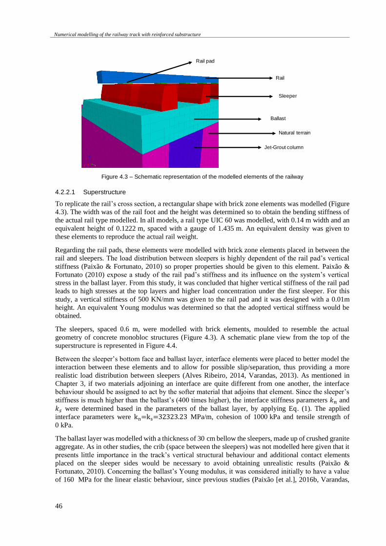
Numerical modelling of the railway track with reinforced substructure
46
Figure 4.3 – Schematic representation of the modelled elements of the railway
4.2.2.1 Superstructure
To replicate the rail’s cross section, a rectangular shape with brick zone elements was modelled (Figure
4.3). The width was of the rail foot and the height was determined so to obtain the bending stiffness of
the actual rail type modelled. In all models, a rail type UIC 60 was modelled, with 0.14 m width and an
equivalent height of 0.1222 m, spaced with a gauge of 1.435 m. An equivalent density was given to
these elements to reproduce the actual rail weight.
Regarding the rail pads, these elements were modelled with brick zone elements placed in between the
rail and sleepers. The load distribution between sleepers is highly dependent of the rail pad’s vertical
stiffness (Paixão & Fortunato, 2010) so proper properties should be given to this element. Paixão &
Fortunato (2010) expose a study of the rail pad’s stiffness and its influence on the system’s vertical
stress in the ballast layer. From this study, it was concluded that higher vertical stiffness of the rail pad
leads to high stresses at the top layers and higher load concentration under the first sleeper. For this
study, a vertical stiffness of 500 KN/mm was given to the rail pad and it was designed with a 0.01m
height. An equivalent Young modulus was determined so that the adopted vertical stiffness would be
obtained.
The sleepers, spaced 0.6 m, were modelled with brick elements, moulded to resemble the actual
geometry of concrete monobloc structures (Figure 4.3). A schematic plane view from the top of the
superstructure is represented in Figure 4.4.
Between the sleeper’s bottom face and ballast layer, interface elements were placed to better model the
interaction between these elements and to allow for possible slip/separation, thus providing a more
realistic load distribution between sleepers (Alves Ribeiro, 2014, Varandas, 2013). As mentioned in
Chapter 3, if two materials adjoining an interface are quite different from one another, the interface
behaviour should be assigned to act by the softer material that adjoins that element. Since the sleeper’s
stiffness is much higher than the ballast’s (400 times higher), the interface stiffness parameters 𝑘𝑛 and
𝑘𝑠 were determined based in the parameters of the ballast layer, by applying Eq. (1). The applied
interface parameters were kn=ks=32323.23 MPa/m, cohesion of 1000 kPa and tensile strength of
0 kPa.
The ballast layer was modelled with a thickness of 30 cm bellow the sleepers, made up of crushed granite
aggregate. As in other studies, the crib (space between the sleepers) was not modelled here given that it
presents little importance in the track’s vertical structural behaviour and additional contact elements
placed on the sleeper sides would be necessary to avoid obtaining unrealistic results (Paixão &
Fortunato, 2010). Concerning the ballast’s Young modulus, it was considered initially to have a value
of 160 MPa for the linear elastic behaviour, since previous studies (Paixão [et al.], 2016b, Varandas,
Rail pad
Rail
Sleeper
Ballast
Natural terrain
Jet-Grout column
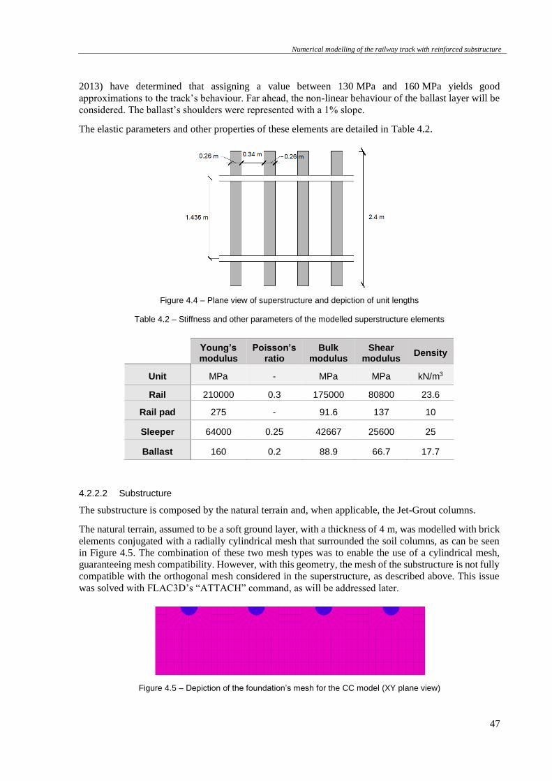
Numerical modelling of the railway track with reinforced substructure
47
2013) have determined that assigning a value between 130 MPa and 160 MPa yields good
approximations to the track’s behaviour. Far ahead, the non-linear behaviour of the ballast layer will be
considered. The ballast’s shoulders were represented with a 1% slope.
The elastic parameters and other properties of these elements are detailed in Table 4.2.
Figure 4.4 – Plane view of superstructure and depiction of unit lengths
Table 4.2 – Stiffness and other parameters of the modelled superstructure elements
4.2.2.2 Substructure
The substructure is composed by the natural terrain and, when applicable, the Jet-Grout columns.
The natural terrain, assumed to be a soft ground layer, with a thickness of 4 m, was modelled with brick
elements conjugated with a radially cylindrical mesh that surrounded the soil columns, as can be seen
in Figure 4.5. The combination of these two mesh types was to enable the use of a cylindrical mesh,
guaranteeing mesh compatibility. However, with this geometry, the mesh of the substructure is not fully
compatible with the orthogonal mesh considered in the superstructure, as described above. This issue
was solved with FLAC3D’s “ATTACH” command, as will be addressed later.
Figure 4.5 – Depiction of the foundation’s mesh for the CC model (XY plane view)
Young’s modulus
Poisson’s ratio
Bulk modulus
Shear modulus
Density
Unit MPa - MPa MPa kN/m3
Rail 210000 0.3 175000 80800 23.6
Rail pad 275 - 91.6 137 10
Sleeper 64000 0.25 42667 25600 25
Ballast 160 0.2 88.9 66.7 17.7
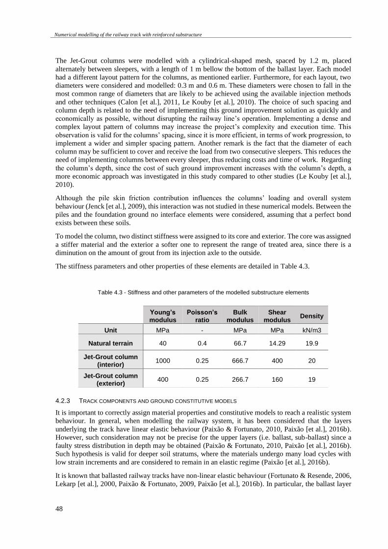
Numerical modelling of the railway track with reinforced substructure
48
The Jet-Grout columns were modelled with a cylindrical-shaped mesh, spaced by 1.2 m, placed
alternately between sleepers, with a length of 1 m bellow the bottom of the ballast layer. Each model
had a different layout pattern for the columns, as mentioned earlier. Furthermore, for each layout, two
diameters were considered and modelled: 0.3 m and 0.6 m. These diameters were chosen to fall in the
most common range of diameters that are likely to be achieved using the available injection methods
and other techniques (Calon [et al.], 2011, Le Kouby [et al.], 2010). The choice of such spacing and
column depth is related to the need of implementing this ground improvement solution as quickly and
economically as possible, without disrupting the railway line’s operation. Implementing a dense and
complex layout pattern of columns may increase the project’s complexity and execution time. This
observation is valid for the columns’ spacing, since it is more efficient, in terms of work progression, to
implement a wider and simpler spacing pattern. Another remark is the fact that the diameter of each
column may be sufficient to cover and receive the load from two consecutive sleepers. This reduces the
need of implementing columns between every sleeper, thus reducing costs and time of work. Regarding
the column’s depth, since the cost of such ground improvement increases with the column’s depth, a
more economic approach was investigated in this study compared to other studies (Le Kouby [et al.],
2010).
Although the pile skin friction contribution influences the columns’ loading and overall system
behaviour (Jenck [et al.], 2009), this interaction was not studied in these numerical models. Between the
piles and the foundation ground no interface elements were considered, assuming that a perfect bond
exists between these soils.
To model the column, two distinct stiffness were assigned to its core and exterior. The core was assigned
a stiffer material and the exterior a softer one to represent the range of treated area, since there is a
diminution on the amount of grout from its injection axle to the outside.
The stiffness parameters and other properties of these elements are detailed in Table 4.3.
Table 4.3 - Stiffness and other parameters of the modelled substructure elements
4.2.3 TRACK COMPONENTS AND GROUND CONSTITUTIVE MODELS
It is important to correctly assign material properties and constitutive models to reach a realistic system
behaviour. In general, when modelling the railway system, it has been considered that the layers
underlying the track have linear elastic behaviour (Paixão & Fortunato, 2010, Paixão [et al.], 2016b).
However, such consideration may not be precise for the upper layers (i.e. ballast, sub-ballast) since a
faulty stress distribution in depth may be obtained (Paixão & Fortunato, 2010, Paixão [et al.], 2016b).
Such hypothesis is valid for deeper soil stratums, where the materials undergo many load cycles with
low strain increments and are considered to remain in an elastic regime (Paixão [et al.], 2016b).
It is known that ballasted railway tracks have non-linear elastic behaviour (Fortunato & Resende, 2006,
Lekarp [et al.], 2000, Paixão & Fortunato, 2009, Paixão [et al.], 2016b). In particular, the ballast layer
Young’s
modulus
Poisson’s
ratio
Bulk
modulus
Shear
modulus Density
Unit MPa - MPa MPa kN/m3
Natural terrain 40 0.4 66.7 14.29 19.9
Jet-Grout column
(interior) 1000 0.25 666.7 400 20
Jet-Grout column (exterior)
400 0.25 266.7 160 19
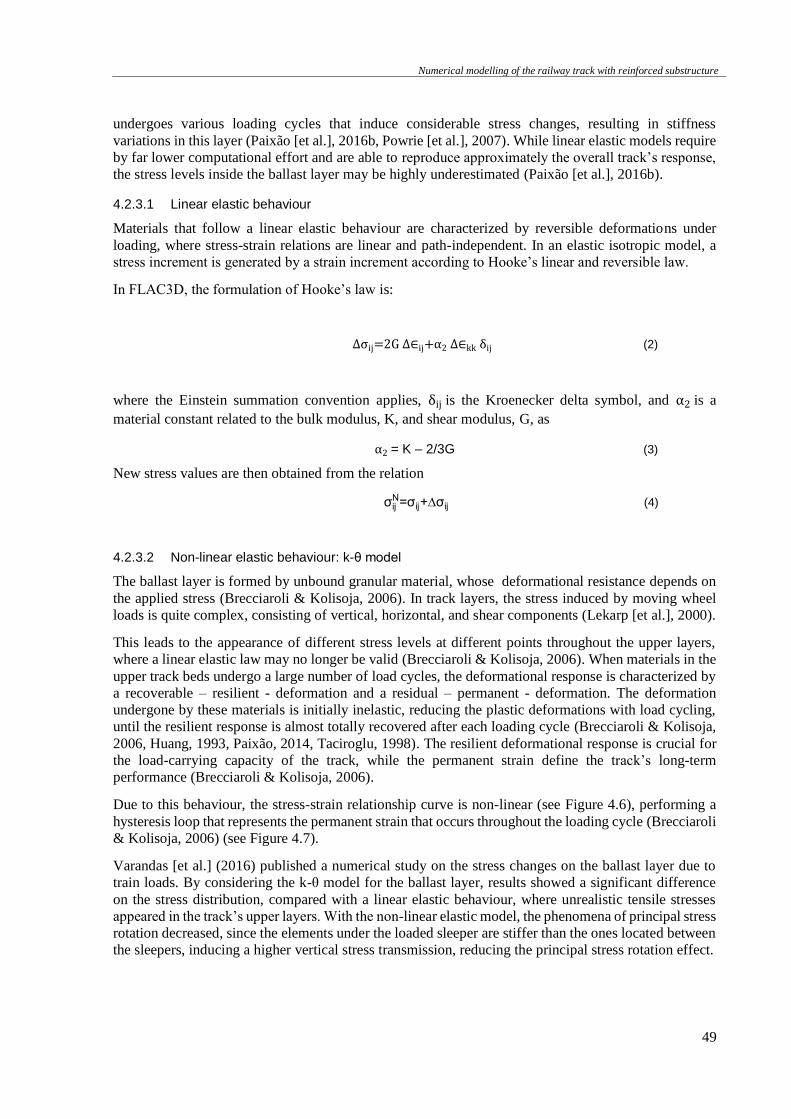
Numerical modelling of the railway track with reinforced substructure
49
undergoes various loading cycles that induce considerable stress changes, resulting in stiffness
variations in this layer (Paixão [et al.], 2016b, Powrie [et al.], 2007). While linear elastic models require
by far lower computational effort and are able to reproduce approximately the overall track’s response,
the stress levels inside the ballast layer may be highly underestimated (Paixão [et al.], 2016b).
4.2.3.1 Linear elastic behaviour
Materials that follow a linear elastic behaviour are characterized by reversible deformations under
loading, where stress-strain relations are linear and path-independent. In an elastic isotropic model, a
stress increment is generated by a strain increment according to Hooke’s linear and reversible law.
In FLAC3D, the formulation of Hooke’s law is:
∆σij=2G ∆∈ij+α2 ∆∈kk δij (2)
where the Einstein summation convention applies, δij is the Kroenecker delta symbol, and α2 is a
material constant related to the bulk modulus, K, and shear modulus, G, as
α2 = K – 2/3G (3)
New stress values are then obtained from the relation
σijN=σij+∆σij (4)
4.2.3.2 Non-linear elastic behaviour: k-θ model
The ballast layer is formed by unbound granular material, whose deformational resistance depends on
the applied stress (Brecciaroli & Kolisoja, 2006). In track layers, the stress induced by moving wheel
loads is quite complex, consisting of vertical, horizontal, and shear components (Lekarp [et al.], 2000).
This leads to the appearance of different stress levels at different points throughout the upper layers,
where a linear elastic law may no longer be valid (Brecciaroli & Kolisoja, 2006). When materials in the
upper track beds undergo a large number of load cycles, the deformational response is characterized by
a recoverable – resilient - deformation and a residual – permanent - deformation. The deformation
undergone by these materials is initially inelastic, reducing the plastic deformations with load cycling,
until the resilient response is almost totally recovered after each loading cycle (Brecciaroli & Kolisoja,
2006, Huang, 1993, Paixão, 2014, Taciroglu, 1998). The resilient deformational response is crucial for
the load-carrying capacity of the track, while the permanent strain define the track’s long-term
performance (Brecciaroli & Kolisoja, 2006).
Due to this behaviour, the stress-strain relationship curve is non-linear (see Figure 4.6), performing a
hysteresis loop that represents the permanent strain that occurs throughout the loading cycle (Brecciaroli
& Kolisoja, 2006) (see Figure 4.7).
Varandas [et al.] (2016) published a numerical study on the stress changes on the ballast layer due to
train loads. By considering the k-θ model for the ballast layer, results showed a significant difference
on the stress distribution, compared with a linear elastic behaviour, where unrealistic tensile stresses
appeared in the track’s upper layers. With the non-linear elastic model, the phenomena of principal stress
rotation decreased, since the elements under the loaded sleeper are stiffer than the ones located between
the sleepers, inducing a higher vertical stress transmission, reducing the principal stress rotation effect.
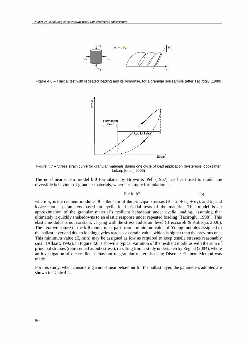
Numerical modelling of the railway track with reinforced substructure
50
Figure 4.6 – Triaxial test with repeated loading and its response, for a granular soil sample (after Taciroglu ,1998)
Figure 4.7 – Stress strain curve for granular materials during one cycle of load application (hysteresis loop) (after Lekarp [et al.],2000)
The non-linear elastic model k-θ formulated by Brown & Pell (1967) has been used to model the
reversible behaviour of granular materials, where its simple formulation is:
Er= k1 θk2 (5)
where Er is the resilient modulus, θ is the sum of the principal stresses (θ = σ1 + σ2 + σ3), and k1 and
k2 are model parameters based on cyclic load triaxial tests of the material. This model is an
approximation of the granular material’s resilient behaviour under cyclic loading, assuming that
ultimately it quickly shakedowns to an elastic response under repeated loading (Taciroglu, 1998). This
elastic modulus is not constant, varying with the stress and strain level (Brecciaroli & Kolisoja, 2006).
The iterative nature of the k-θ model must part from a minimum value of Young modulus assigned to
the ballast layer and due to loading cycles reaches a certain value, which is higher than the previous one.
This minimum value (Er min ) may be assigned as low as required to keep tensile stresses reasonably
small (Allaart, 1992). In Figure 4.8 is shown a typical variation of the resilient modulus with the sum of
principal stresses (represented as bulk stress), resulting from a study undertaken by Zeghal (2004), where
an investigation of the resilient behaviour of granular materials using Discrete-Element Method was
made.
For this study, when considering a non-linear behaviour for the ballast layer, the parameters adopted are
shown in Table 4.4.
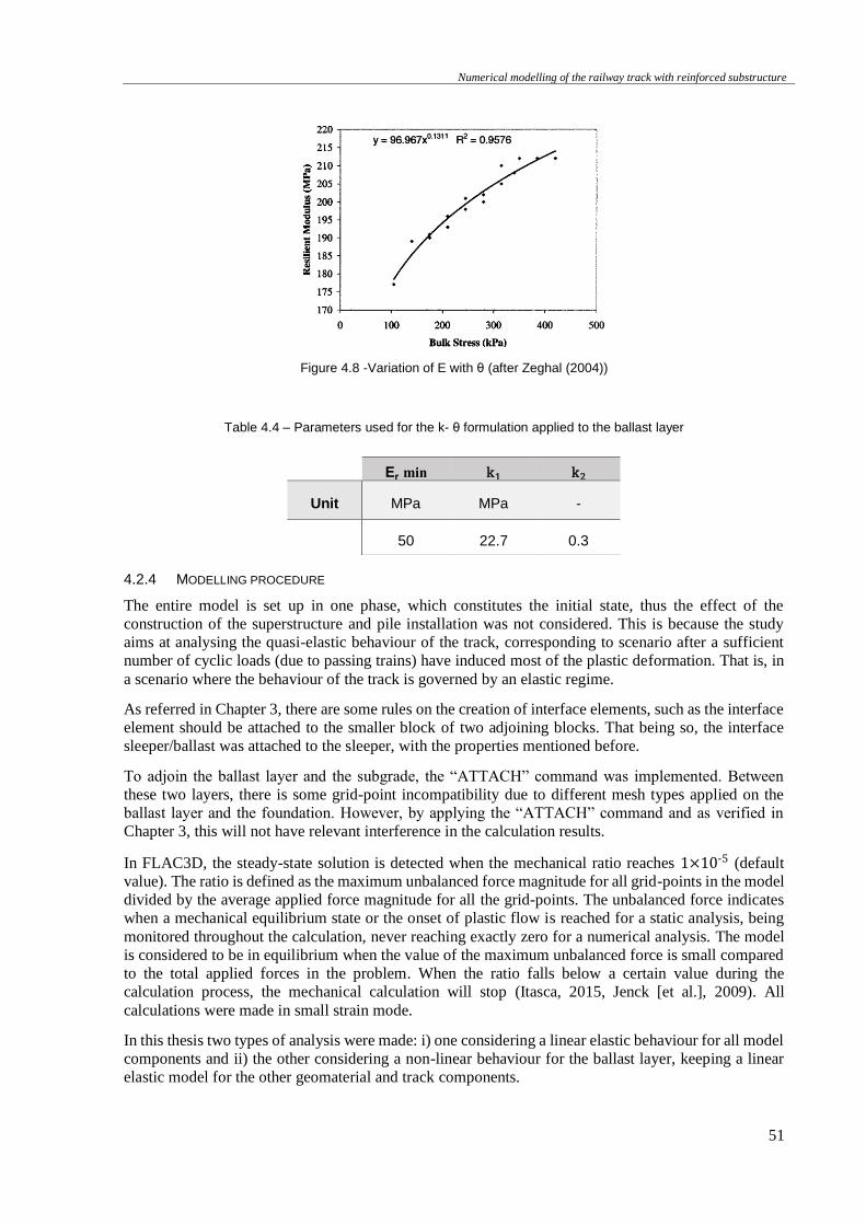
Numerical modelling of the railway track with reinforced substructure
51
Figure 4.8 -Variation of E with θ (after Zeghal (2004))
Table 4.4 – Parameters used for the k- θ formulation applied to the ballast layer
4.2.4 MODELLING PROCEDURE
The entire model is set up in one phase, which constitutes the initial state, thus the effect of the
construction of the superstructure and pile installation was not considered. This is because the study
aims at analysing the quasi-elastic behaviour of the track, corresponding to scenario after a sufficient
number of cyclic loads (due to passing trains) have induced most of the plastic deformation. That is, in
a scenario where the behaviour of the track is governed by an elastic regime.
As referred in Chapter 3, there are some rules on the creation of interface elements, such as the interface
element should be attached to the smaller block of two adjoining blocks. That being so, the interface
sleeper/ballast was attached to the sleeper, with the properties mentioned before.
To adjoin the ballast layer and the subgrade, the “ATTACH” command was implemented. Between
these two layers, there is some grid-point incompatibility due to different mesh types applied on the
ballast layer and the foundation. However, by applying the “ATTACH” command and as verified in
Chapter 3, this will not have relevant interference in the calculation results.
In FLAC3D, the steady-state solution is detected when the mechanical ratio reaches 1×10⁻⁵ (default
value). The ratio is defined as the maximum unbalanced force magnitude for all grid-points in the model
divided by the average applied force magnitude for all the grid-points. The unbalanced force indicates
when a mechanical equilibrium state or the onset of plastic flow is reached for a static analysis, being
monitored throughout the calculation, never reaching exactly zero for a numerical analysis. The model
is considered to be in equilibrium when the value of the maximum unbalanced force is small compared
to the total applied forces in the problem. When the ratio falls below a certain value during the
calculation process, the mechanical calculation will stop (Itasca, 2015, Jenck [et al.], 2009). All
calculations were made in small strain mode.
In this thesis two types of analysis were made: i) one considering a linear elastic behaviour for all model
components and ii) the other considering a non-linear behaviour for the ballast layer, keeping a linear
elastic model for the other geomaterial and track components.
Er min k1 k2
Unit MPa MPa -
50 22.7 0.3
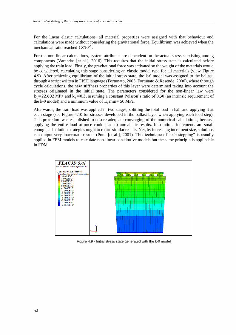
Numerical modelling of the railway track with reinforced substructure
52
For the linear elastic calculations, all material properties were assigned with that behaviour and
calculations were made without considering the gravitational force. Equilibrium was achieved when the
mechanical ratio reached 1×10⁻⁵.
For the non-linear calculations, system attributes are dependent on the actual stresses existing among
components (Varandas [et al.], 2016). This requires that the initial stress state is calculated before
applying the train load. Firstly, the gravitational force was activated so the weight of the materials would
be considered, calculating this stage considering an elastic model type for all materials (view Figure
4.9). After achieving equilibrium of the initial stress state, the k-θ model was assigned to the ballast,
through a script written in FISH language (Fortunato, 2005, Fortunato & Resende, 2006), where through
cycle calculations, the new stiffness properties of this layer were determined taking into account the
stresses originated in the initial state. The parameters considered for the non-linear law were
k1=22.682 MPa and k2=0.3, assuming a constant Poisson’s ratio of 0.30 (an intrinsic requirement of
the k-θ model) and a minimum value of Er min = 50 MPa.
Afterwards, the train load was applied in two stages, splitting the total load in half and applying it at
each stage (see Figure 4.10 for stresses developed in the ballast layer when applying each load step).
This procedure was established to ensure adequate converging of the numerical calculations, because
applying the entire load at once could lead to unrealistic results. If solutions increments are small
enough, all solution strategies ought to return similar results. Yet, by increasing increment size, solutions
can output very inaccurate results (Potts [et al.], 2001). This technique of “sub stepping” is usually
applied in FEM models to calculate non-linear constitutive models but the same principle is applicable
in FDM.
Figure 4.9 - Initial stress state generated with the k-θ model
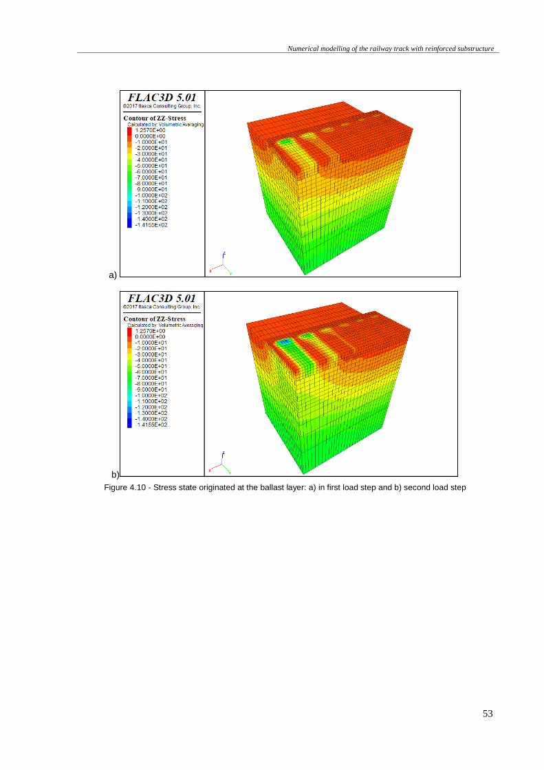
Numerical modelling of the railway track with reinforced substructure
53
a)
b)
Figure 4.10 - Stress state originated at the ballast layer: a) in first load step and b) second load step

Numerical modelling of the railway track with reinforced substructure
54
Numerical modelling of the railway track with reinforced substructure
55
PARAMETRIC STUDY ON THE
STRUCTURAL BEHAVIOUR OF RAILWAY TRACKS WITH
REINFORCED SUBSTRUCTURE
5.1 GENERAL ASPECTS
To evaluate the potential of subgrade improvement by means of Jet-grout columns, various layouts with
different placement patterns of the columns within the subgrade were designed and studied, generating
different structures. In this chapter, the results of a parametric study on the influence of the column
diameter, column pattern and loading position are presented and discussed to obtain more insight into
the behaviour of these structures and to assess the advantages and potentiality of this ground
improvement technique.
The generated models were designed as described in Chapter 4. The parametric study also focused on
analysing the influence of assigning non-linear elastic constitutive behaviour to some geomaterials to
achieve a more realistic representation of the actual behaviour of the track system. Firstly, results
considering the linear elastic behaviour only will be analysed and discussed. Then, the non-linear elastic
behaviour will be introduced in the ballast layer following a k-θ law and subsequent analysis and
discussion of the results will be presented. This chapter will conclude with a comparison between these
two approaches and an overall summary of results.
In general, the analysis of results was made in terms of vertical stress and vertical displacement values.
The rail’s vertical displacements, as well as the displacements and stresses developed in depth in the
geomaterials, were analysed at the XZ plane aligned with the rail. The stresses and displacements on the
top and at the bottom of the ballast layer, on the top of the foundation and slightly beneath the Jet column
were analysed at specific XY planes, (see Figure 5.1).
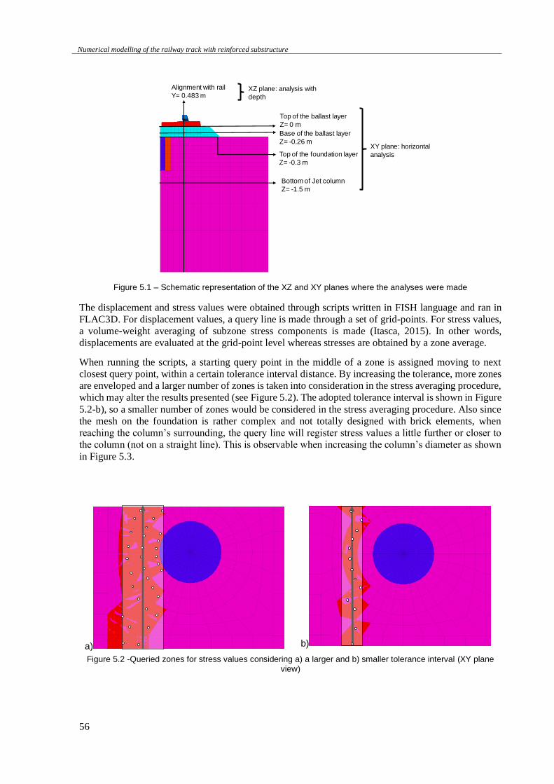
Numerical modelling of the railway track with reinforced substructure
56
Figure 5.1 – Schematic representation of the XZ and XY planes where the analyses were made
The displacement and stress values were obtained through scripts written in FISH language and ran in
FLAC3D. For displacement values, a query line is made through a set of grid-points. For stress values,
a volume-weight averaging of subzone stress components is made (Itasca, 2015). In other words,
displacements are evaluated at the grid-point level whereas stresses are obtained by a zone average.
When running the scripts, a starting query point in the middle of a zone is assigned moving to next
closest query point, within a certain tolerance interval distance. By increasing the tolerance, more zones
are enveloped and a larger number of zones is taken into consideration in the stress averaging procedure,
which may alter the results presented (see Figure 5.2). The adopted tolerance interval is shown in Figure
5.2-b), so a smaller number of zones would be considered in the stress averaging procedure. Also since
the mesh on the foundation is rather complex and not totally designed with brick elements, when
reaching the column’s surrounding, the query line will register stress values a little further or closer to
the column (not on a straight line). This is observable when increasing the column’s diameter as shown
in Figure 5.3.
a) b)
Figure 5.2 -Queried zones for stress values considering a) a larger and b) smaller tolerance interval (XY plane view)
Top of the ballast layer
Z= 0 m
Top of the foundation layer
Z= -0.3 m
Alignment with rail
Y= 0.483 mXZ plane: analysis with
depth
XY plane: horizontal
analysis
Bottom of Jet column
Z= -1.5 m
Base of the ballast layer
Z= -0.26 m
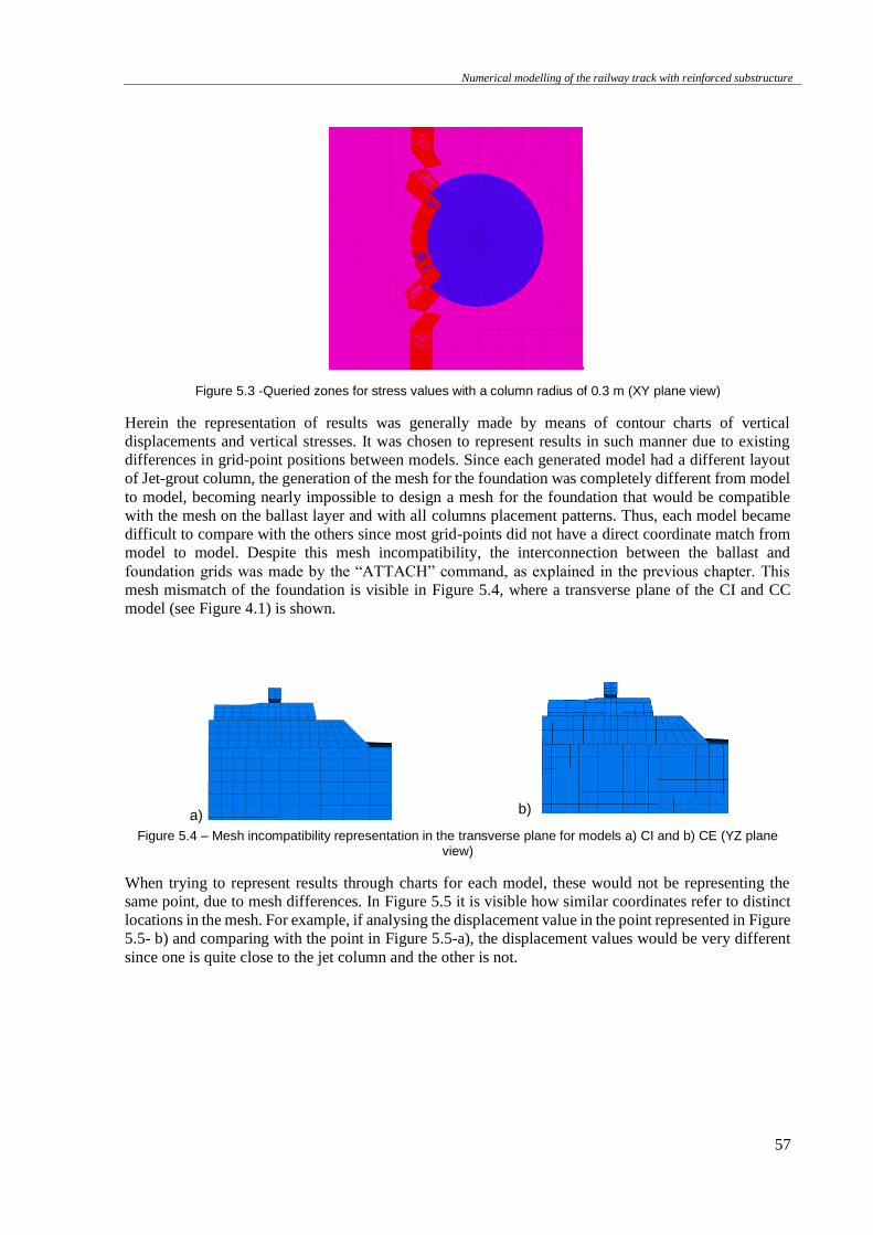
Numerical modelling of the railway track with reinforced substructure
57
Figure 5.3 -Queried zones for stress values with a column radius of 0.3 m (XY plane view)
Herein the representation of results was generally made by means of contour charts of vertical
displacements and vertical stresses. It was chosen to represent results in such manner due to existing
differences in grid-point positions between models. Since each generated model had a different layout
of Jet-grout column, the generation of the mesh for the foundation was completely different from model
to model, becoming nearly impossible to design a mesh for the foundation that would be compatible
with the mesh on the ballast layer and with all columns placement patterns. Thus, each model became
difficult to compare with the others since most grid-points did not have a direct coordinate match from
model to model. Despite this mesh incompatibility, the interconnection between the ballast and
foundation grids was made by the “ATTACH” command, as explained in the previous chapter. This
mesh mismatch of the foundation is visible in Figure 5.4, where a transverse plane of the CI and CC
model (see Figure 4.1) is shown.
a) b)
Figure 5.4 – Mesh incompatibility representation in the transverse plane for models a) CI and b) CE (YZ plane view)
When trying to represent results through charts for each model, these would not be representing the
same point, due to mesh differences. In Figure 5.5 it is visible how similar coordinates refer to distinct
locations in the mesh. For example, if analysing the displacement value in the point represented in Figure
5.5- b) and comparing with the point in Figure 5.5-a), the displacement values would be very different
since one is quite close to the jet column and the other is not.
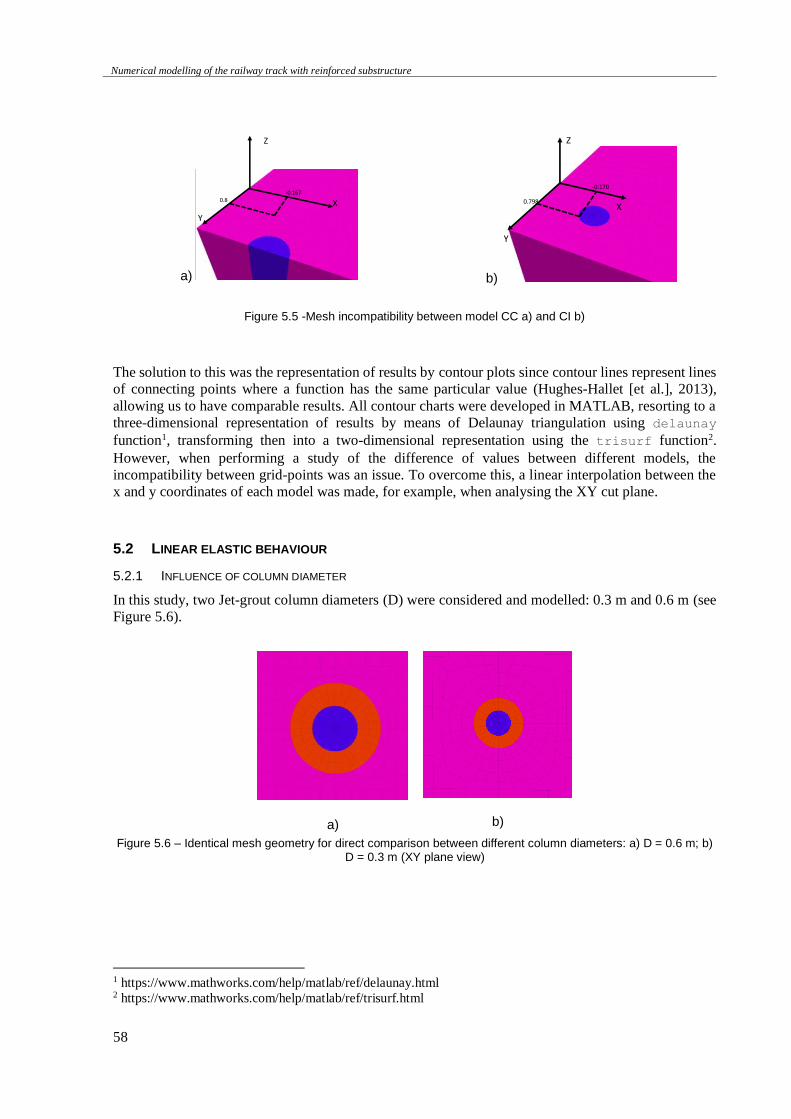
Numerical modelling of the railway track with reinforced substructure
58
a) b)
Figure 5.5 -Mesh incompatibility between model CC a) and CI b)
The solution to this was the representation of results by contour plots since contour lines represent lines
of connecting points where a function has the same particular value (Hughes-Hallet [et al.], 2013),
allowing us to have comparable results. All contour charts were developed in MATLAB, resorting to a
three-dimensional representation of results by means of Delaunay triangulation using delaunay
function1, transforming then into a two-dimensional representation using the trisurf function2.
However, when performing a study of the difference of values between different models, the
incompatibility between grid-points was an issue. To overcome this, a linear interpolation between the
x and y coordinates of each model was made, for example, when analysing the XY cut plane.
5.2 LINEAR ELASTIC BEHAVIOUR
5.2.1 INFLUENCE OF COLUMN DIAMETER
In this study, two Jet-grout column diameters (D) were considered and modelled: 0.3 m and 0.6 m (see
Figure 5.6).
a)
b)
Figure 5.6 – Identical mesh geometry for direct comparison between different column diameters: a) D = 0.6 m; b) D = 0.3 m (XY plane view)
1 https://www.mathworks.com/help/matlab/ref/delaunay.html 2 https://www.mathworks.com/help/matlab/ref/trisurf.html
Z
Y
X-0.167
0.8
Z
Y
X
-0.170
0.798
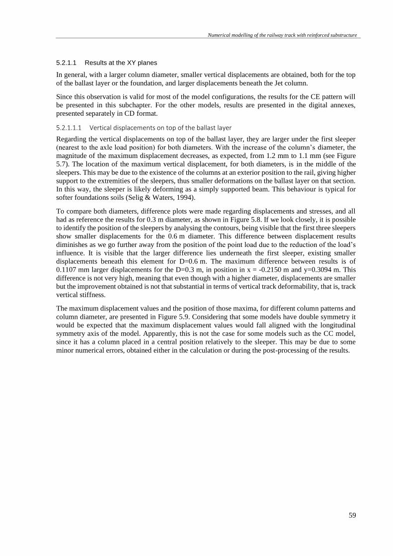
Numerical modelling of the railway track with reinforced substructure
59
5.2.1.1 Results at the XY planes
In general, with a larger column diameter, smaller vertical displacements are obtained, both for the top
of the ballast layer or the foundation, and larger displacements beneath the Jet column.
Since this observation is valid for most of the model configurations, the results for the CE pattern will
be presented in this subchapter. For the other models, results are presented in the digital annexes,
presented separately in CD format.
5.2.1.1.1 Vertical displacements on top of the ballast layer
Regarding the vertical displacements on top of the ballast layer, they are larger under the first sleeper
(nearest to the axle load position) for both diameters. With the increase of the column’s diameter, the
magnitude of the maximum displacement decreases, as expected, from 1.2 mm to 1.1 mm (see Figure
5.7). The location of the maximum vertical displacement, for both diameters, is in the middle of the
sleepers. This may be due to the existence of the columns at an exterior position to the rail, giving higher
support to the extremities of the sleepers, thus smaller deformations on the ballast layer on that section.
In this way, the sleeper is likely deforming as a simply supported beam. This behaviour is typical for
softer foundations soils (Selig & Waters, 1994).
To compare both diameters, difference plots were made regarding displacements and stresses, and all
had as reference the results for 0.3 m diameter, as shown in Figure 5.8. If we look closely, it is possible
to identify the position of the sleepers by analysing the contours, being visible that the first three sleepers
show smaller displacements for the 0.6 m diameter. This difference between displacement results
diminishes as we go further away from the position of the point load due to the reduction of the load’s
influence. It is visible that the larger difference lies underneath the first sleeper, existing smaller
displacements beneath this element for D=0.6 m. The maximum difference between results is of
0.1107 mm larger displacements for the D=0.3 m, in position in x = -0.2150 m and y=0.3094 m. This
difference is not very high, meaning that even though with a higher diameter, displacements are smaller
but the improvement obtained is not that substantial in terms of vertical track deformability, that is, track
vertical stiffness.
The maximum displacement values and the position of those maxima, for different column patterns and
column diameter, are presented in Figure 5.9. Considering that some models have double symmetry it
would be expected that the maximum displacement values would fall aligned with the longitudinal
symmetry axis of the model. Apparently, this is not the case for some models such as the CC model,
since it has a column placed in a central position relatively to the sleeper. This may be due to some
minor numerical errors, obtained either in the calculation or during the post-processing of the results.
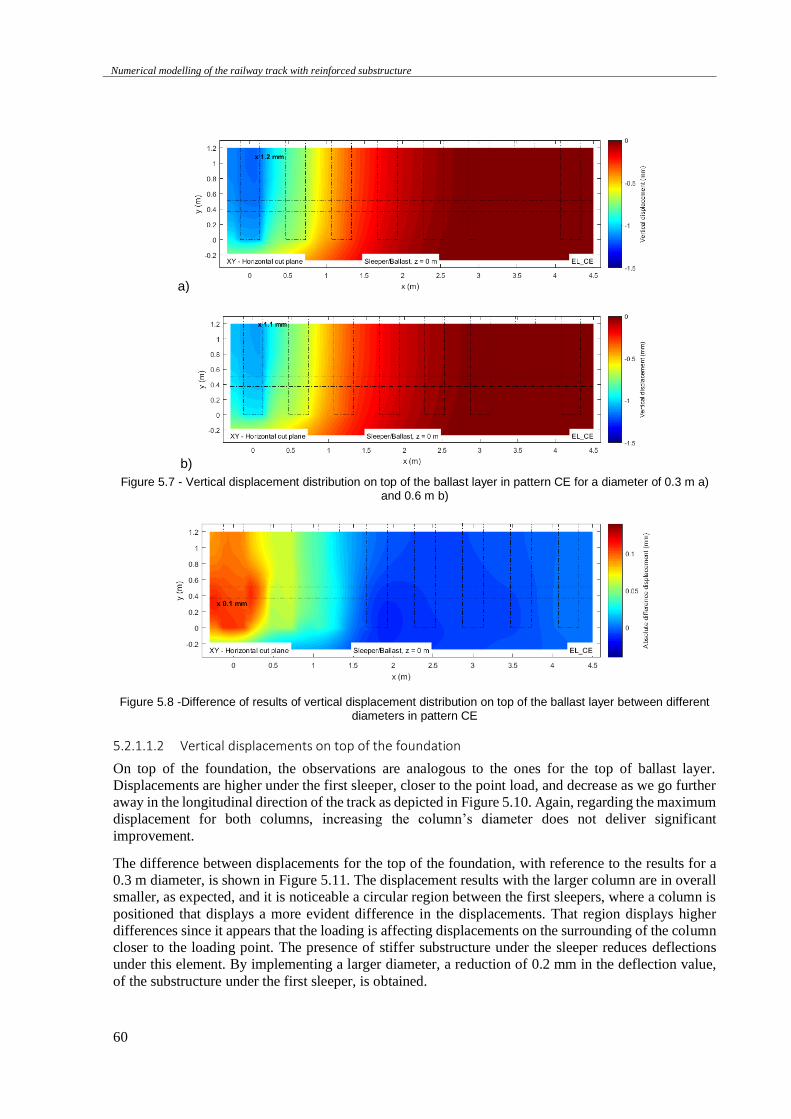
Numerical modelling of the railway track with reinforced substructure
60
a)
b)
Figure 5.7 - Vertical displacement distribution on top of the ballast layer in pattern CE for a diameter of 0.3 m a) and 0.6 m b)
Figure 5.8 -Difference of results of vertical displacement distribution on top of the ballast layer between different diameters in pattern CE
5.2.1.1.2 Vertical displacements on top of the foundation
On top of the foundation, the observations are analogous to the ones for the top of ballast layer.
Displacements are higher under the first sleeper, closer to the point load, and decrease as we go further
away in the longitudinal direction of the track as depicted in Figure 5.10. Again, regarding the maximum
displacement for both columns, increasing the column’s diameter does not deliver significant
improvement.
The difference between displacements for the top of the foundation, with reference to the results for a
0.3 m diameter, is shown in Figure 5.11. The displacement results with the larger column are in overall
smaller, as expected, and it is noticeable a circular region between the first sleepers, where a column is
positioned that displays a more evident difference in the displacements. That region displays higher
differences since it appears that the loading is affecting displacements on the surrounding of the column
closer to the loading point. The presence of stiffer substructure under the sleeper reduces deflections
under this element. By implementing a larger diameter, a reduction of 0.2 mm in the deflection value,
of the substructure under the first sleeper, is obtained.
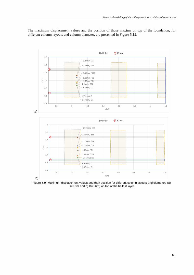
Numerical modelling of the railway track with reinforced substructure
61
The maximum displacement values and the position of those maxima on top of the foundation, for
different column layouts and column diameter, are presented in Figure 5.12.
a)
b)
Figure 5.9 -Maximum displacement values and their position for different column layouts and diameters (a) D=0.3m and b) D=0.6m) on top of the ballast layer.
1.2mm / CC
1.2mm / CC1
1.18mm / CE
1.18mm / CE1
1.17mm / CI
1.17mm / CI1
1.18mm / EZZ
1.17mm / IZZ
1.23mm / N
-0.3
0.2
0.7
1.2
1.7
2.2
2.7
-1.2-1-0.8-0.6-0.4-0.200.2
x (m
)
y (m)
D=0.3m 20 ton
1.14mm / CC
1.14mm / CC1
1.09mm / CE
1.09mm / CE1
1.07mm / CI
1.07mm / CI1
1.09mm / EZZ
1.07mm / IZZ
1.23mm / N
-0.3
0.2
0.7
1.2
1.7
2.2
2.7
-1.2-1-0.8-0.6-0.4-0.200.2
x (m
)
y (m)
D=0.6m 20 ton
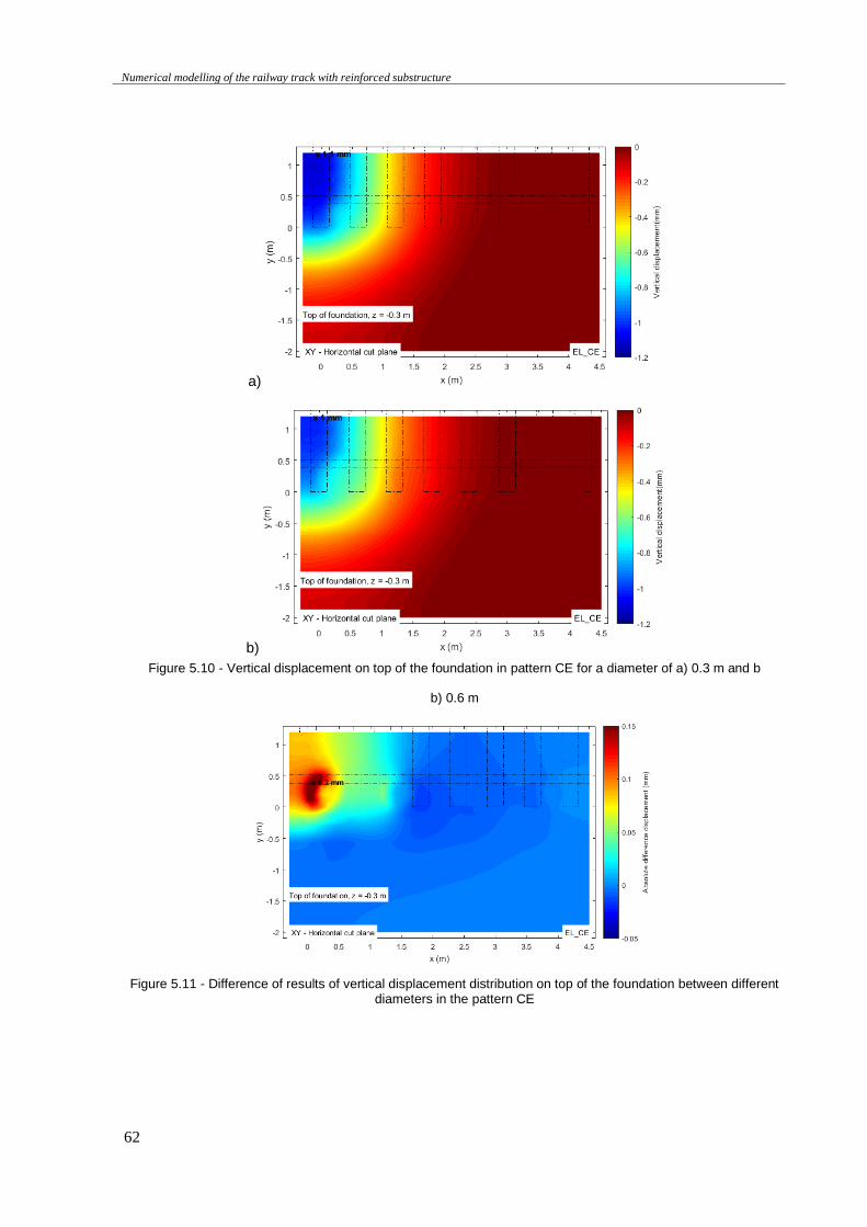
Numerical modelling of the railway track with reinforced substructure
62
a)
b)
Figure 5.10 - Vertical displacement on top of the foundation in pattern CE for a diameter of a) 0.3 m and b
b) 0.6 m
Figure 5.11 - Difference of results of vertical displacement distribution on top of the foundation between different diameters in the pattern CE
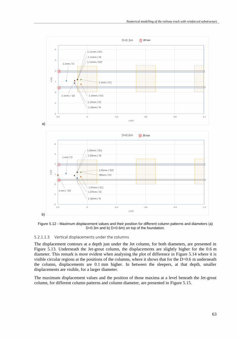
Numerical modelling of the railway track with reinforced substructure
63
a)
b)
Figure 5.12 - Maximum displacement values and their position for different column patterns and diameters (a) D=0.3m and b) D=0.6m) on top of the foundation.
5.2.1.1.3 Vertical displacements under the columns
The displacement contours at a depth just under the Jet column, for both diameters, are presented in
Figure 5.13. Underneath the Jet-grout column, the displacements are slightly higher for the 0.6 m
diameter. This remark is more evident when analysing the plot of difference in Figure 5.14 where it is
visible circular regions at the positions of the columns, where it shows that for the D=0.6 m underneath
the column, displacements are 0.1 mm higher. In between the sleepers, at that depth, smaller
displacements are visible, for a larger diameter.
The maximum displacement values and the position of those maxima at a level beneath the Jet-grout
column, for different column patterns and column diameter, are presented in Figure 5.15.
1.13mm / CC
1.13mm / CC1
1.11mm / CE
1.11mm / CE1
1.1mm / CI
1.1mm / CI1
1.11mm / EZZ
1.1mm / IZZ
1.16mm / N
-2
-1
0
1
2
3
4
-1.2-0.9-0.6-0.300.3
x (m
)
y (m)
D=0.3m 20 ton
1.07mm / CC
1.07mm / CC1
1.03mm / CE
1.03mm / CE1
1.mm / CI
.99mm / CI1
1.03mm / EZZ
1.mm / IZZ
1.16mm / N
-2
-1
0
1
2
3
4
-1.2-0.9-0.6-0.300.3
x (m
)
y (m)
D=0.6m 20 ton
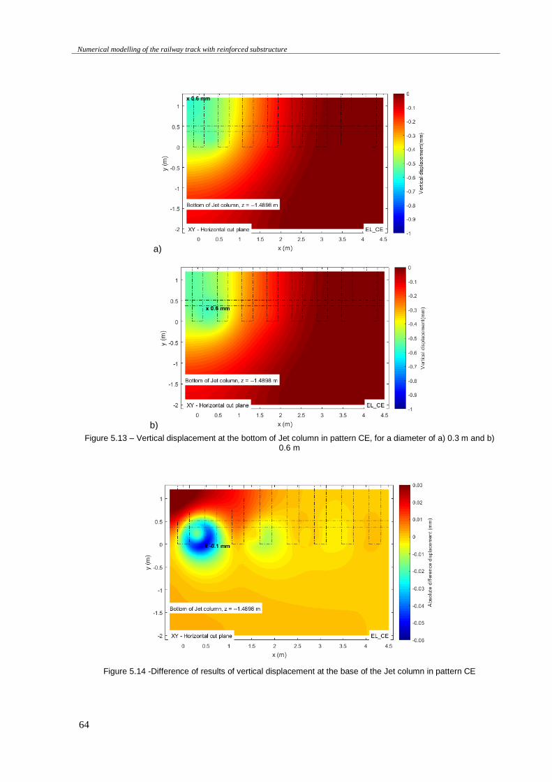
Numerical modelling of the railway track with reinforced substructure
64
a)
b)
Figure 5.13 – Vertical displacement at the bottom of Jet column in pattern CE, for a diameter of a) 0.3 m and b) 0.6 m
Figure 5.14 -Difference of results of vertical displacement at the base of the Jet column in pattern CE
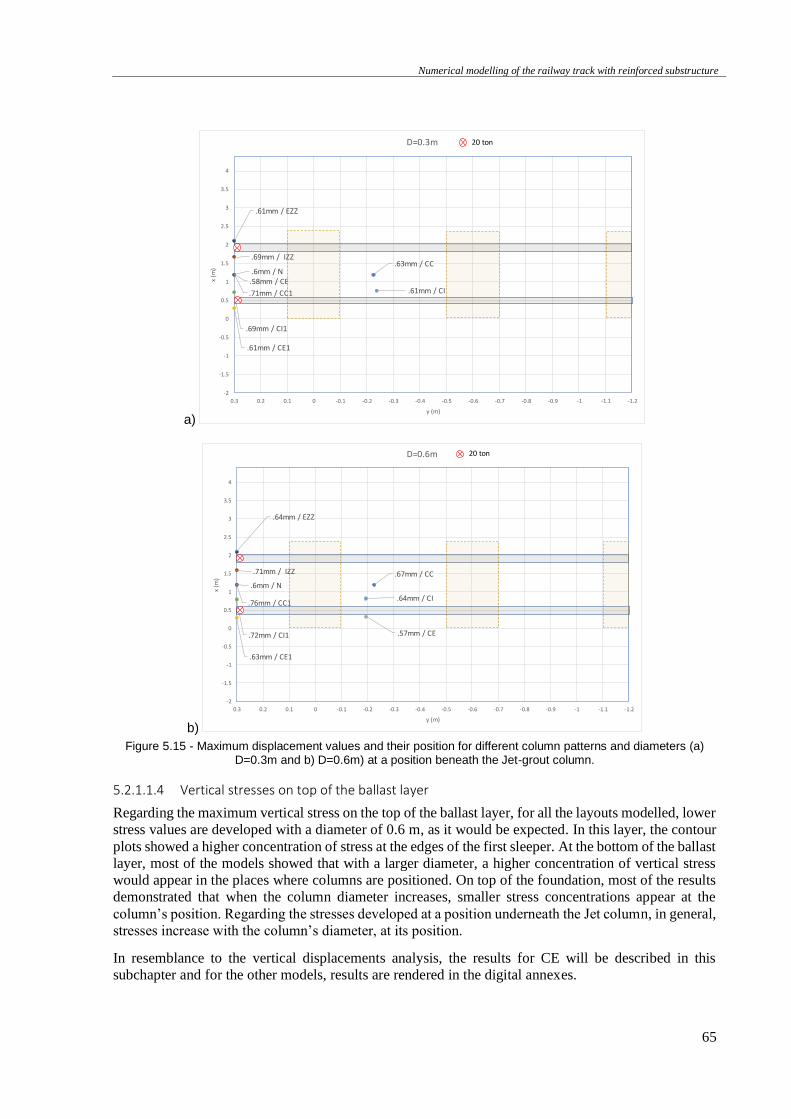
Numerical modelling of the railway track with reinforced substructure
65
a)
b)
Figure 5.15 - Maximum displacement values and their position for different column patterns and diameters (a) D=0.3m and b) D=0.6m) at a position beneath the Jet-grout column.
5.2.1.1.4 Vertical stresses on top of the ballast layer
Regarding the maximum vertical stress on the top of the ballast layer, for all the layouts modelled, lower
stress values are developed with a diameter of 0.6 m, as it would be expected. In this layer, the contour
plots showed a higher concentration of stress at the edges of the first sleeper. At the bottom of the ballast
layer, most of the models showed that with a larger diameter, a higher concentration of vertical stress
would appear in the places where columns are positioned. On top of the foundation, most of the results
demonstrated that when the column diameter increases, smaller stress concentrations appear at the
column’s position. Regarding the stresses developed at a position underneath the Jet column, in general,
stresses increase with the column’s diameter, at its position.
In resemblance to the vertical displacements analysis, the results for CE will be described in this
subchapter and for the other models, results are rendered in the digital annexes.
.63mm / CC
.71mm / CC1
.58mm / CE
.61mm / CE1
.61mm / CI
.69mm / CI1
.61mm / EZZ
.69mm / IZZ
.6mm / N
-2
-1.5
-1
-0.5
0
0.5
1
1.5
2
2.5
3
3.5
4
-1.2-1.1-1-0.9-0.8-0.7-0.6-0.5-0.4-0.3-0.2-0.100.10.20.3
x (m
)
y (m)
D=0.3m 20 ton
.67mm / CC
.76mm / CC1
.57mm / CE
.63mm / CE1
.64mm / CI
.72mm / CI1
.64mm / EZZ
.71mm / IZZ
.6mm / N
-2
-1.5
-1
-0.5
0
0.5
1
1.5
2
2.5
3
3.5
4
-1.2-1.1-1-0.9-0.8-0.7-0.6-0.5-0.4-0.3-0.2-0.100.10.20.3
x (m
)
y (m)
D=0.6m 20 ton
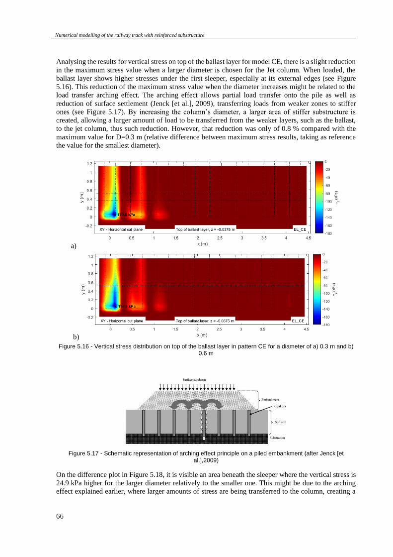
Numerical modelling of the railway track with reinforced substructure
66
Analysing the results for vertical stress on top of the ballast layer for model CE, there is a slight reduction
in the maximum stress value when a larger diameter is chosen for the Jet column. When loaded, the
ballast layer shows higher stresses under the first sleeper, especially at its external edges (see Figure
5.16). This reduction of the maximum stress value when the diameter increases might be related to the
load transfer arching effect. The arching effect allows partial load transfer onto the pile as well as
reduction of surface settlement (Jenck [et al.], 2009), transferring loads from weaker zones to stiffer
ones (see Figure 5.17). By increasing the column’s diameter, a larger area of stiffer substructure is
created, allowing a larger amount of load to be transferred from the weaker layers, such as the ballast,
to the jet column, thus such reduction. However, that reduction was only of 0.8 % compared with the
maximum value for D=0.3 m (relative difference between maximum stress results, taking as reference
the value for the smallest diameter).
a)
b)
Figure 5.16 - Vertical stress distribution on top of the ballast layer in pattern CE for a diameter of a) 0.3 m and b) 0.6 m
Figure 5.17 - Schematic representation of arching effect principle on a piled embankment (after Jenck [et al.],2009)
On the difference plot in Figure 5.18, it is visible an area beneath the sleeper where the vertical stress is
24.9 kPa higher for the larger diameter relatively to the smaller one. This might be due to the arching
effect explained earlier, where larger amounts of stress are being transferred to the column, creating a
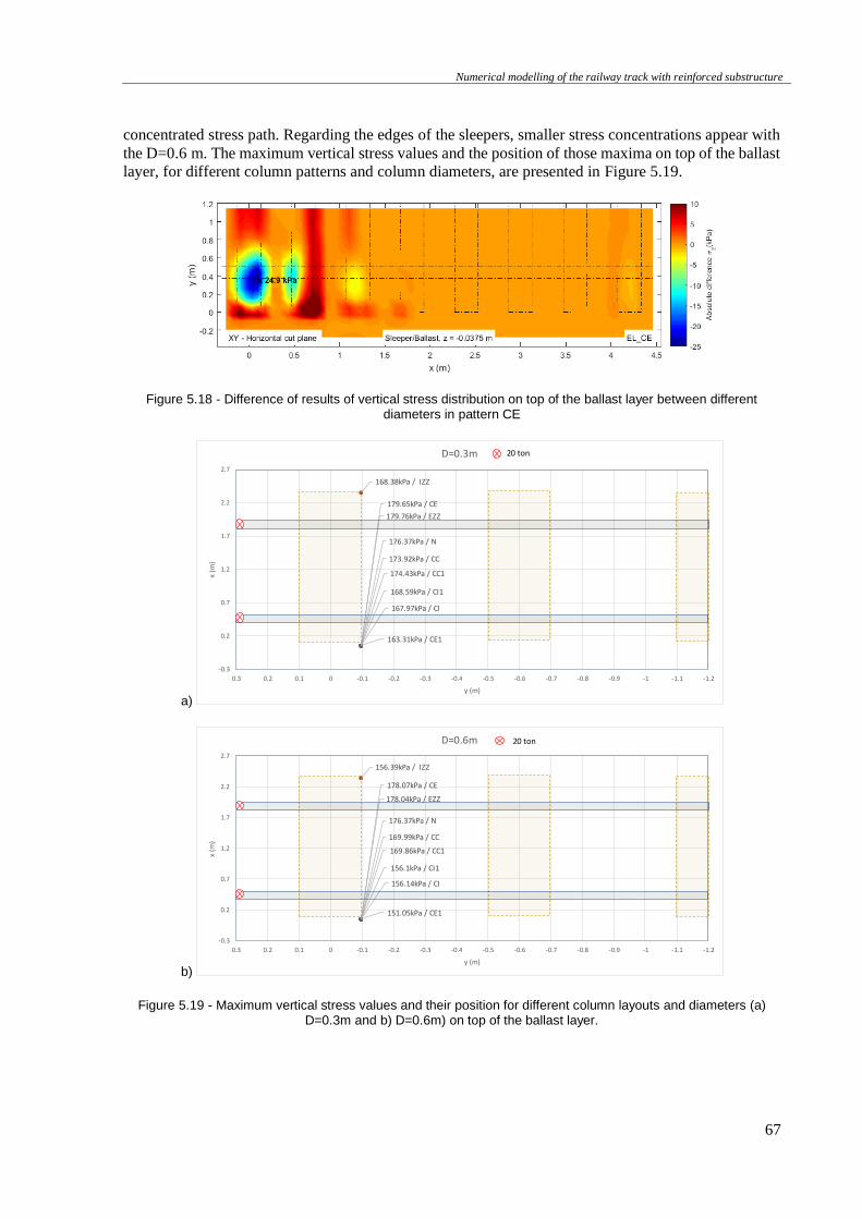
Numerical modelling of the railway track with reinforced substructure
67
concentrated stress path. Regarding the edges of the sleepers, smaller stress concentrations appear with
the D=0.6 m. The maximum vertical stress values and the position of those maxima on top of the ballast
layer, for different column patterns and column diameters, are presented in Figure 5.19.
Figure 5.18 - Difference of results of vertical stress distribution on top of the ballast layer between different diameters in pattern CE
a)
b)
Figure 5.19 - Maximum vertical stress values and their position for different column layouts and diameters (a) D=0.3m and b) D=0.6m) on top of the ballast layer.
173.92kPa / CC
174.43kPa / CC1
179.65kPa / CE
163.31kPa / CE1
167.97kPa / CI
168.59kPa / CI1
179.76kPa / EZZ
168.38kPa / IZZ
176.37kPa / N
-0.3
0.2
0.7
1.2
1.7
2.2
2.7
-1.2-1.1-1-0.9-0.8-0.7-0.6-0.5-0.4-0.3-0.2-0.100.10.20.3
x (m
)
y (m)
D=0.3m 20 ton
169.99kPa / CC
169.86kPa / CC1
178.07kPa / CE
151.05kPa / CE1
156.14kPa / CI
156.1kPa / CI1
178.04kPa / EZZ
156.39kPa / IZZ
176.37kPa / N
-0.3
0.2
0.7
1.2
1.7
2.2
2.7
-1.2-1.1-1-0.9-0.8-0.7-0.6-0.5-0.4-0.3-0.2-0.100.10.20.3
x (m
)
y (m)
D=0.6m 20 ton
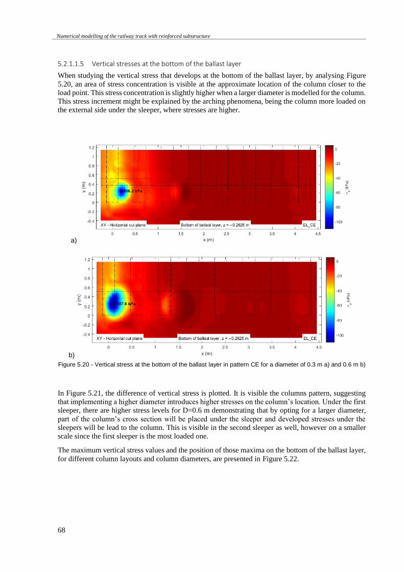
Numerical modelling of the railway track with reinforced substructure
68
5.2.1.1.5 Vertical stresses at the bottom of the ballast layer
When studying the vertical stress that develops at the bottom of the ballast layer, by analysing Figure
5.20, an area of stress concentration is visible at the approximate location of the column closer to the
load point. This stress concentration is slightly higher when a larger diameter is modelled for the column.
This stress increment might be explained by the arching phenomena, being the column more loaded on
the external side under the sleeper, where stresses are higher.
a)
b)
Figure 5.20 - Vertical stress at the bottom of the ballast layer in pattern CE for a diameter of 0.3 m a) and 0.6 m b)
In Figure 5.21, the difference of vertical stress is plotted. It is visible the columns pattern, suggesting
that implementing a higher diameter introduces higher stresses on the column’s location. Under the first
sleeper, there are higher stress levels for D=0.6 m demonstrating that by opting for a larger diameter,
part of the column’s cross section will be placed under the sleeper and developed stresses under the
sleepers will be lead to the column. This is visible in the second sleeper as well, however on a smaller
scale since the first sleeper is the most loaded one.
The maximum vertical stress values and the position of those maxima on the bottom of the ballast layer,
for different column layouts and column diameters, are presented in Figure 5.22.
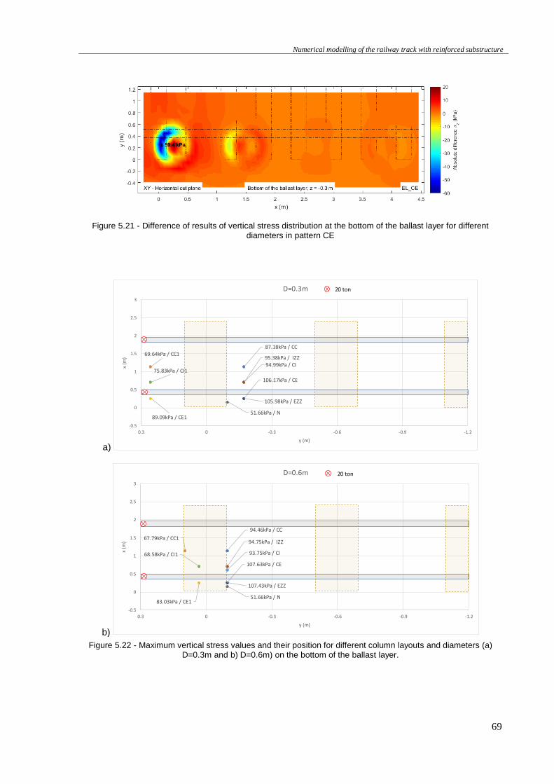
Numerical modelling of the railway track with reinforced substructure
69
Figure 5.21 - Difference of results of vertical stress distribution at the bottom of the ballast layer for different diameters in pattern CE
a)
b)
Figure 5.22 - Maximum vertical stress values and their position for different column layouts and diameters (a) D=0.3m and b) D=0.6m) on the bottom of the ballast layer.
87.18kPa / CC69.64kPa / CC1
106.17kPa / CE
89.09kPa / CE1
94.99kPa / CI75.83kPa / CI1
105.98kPa / EZZ
95.38kPa / IZZ
51.66kPa / N
-0.5
0
0.5
1
1.5
2
2.5
3
-1.2-0.9-0.6-0.300.3
x (m
)
y (m)
D=0.3m 20 ton
94.46kPa / CC
67.79kPa / CC1
107.63kPa / CE
83.03kPa / CE1
93.75kPa / CI68.58kPa / CI1
107.43kPa / EZZ
94.75kPa / IZZ
51.66kPa / N
-0.5
0
0.5
1
1.5
2
2.5
3
-1.2-0.9-0.6-0.300.3
x (m
)
y (m)
D=0.6m 20 ton
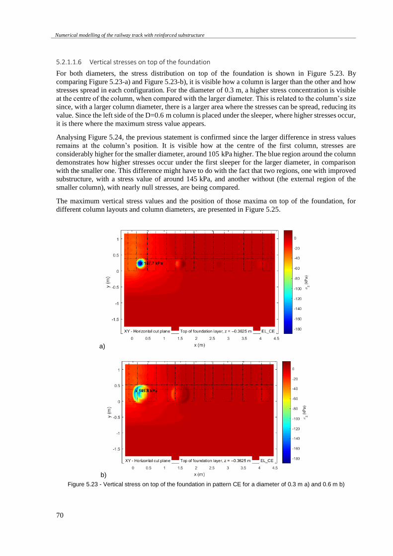
Numerical modelling of the railway track with reinforced substructure
70
5.2.1.1.6 Vertical stresses on top of the foundation
For both diameters, the stress distribution on top of the foundation is shown in Figure 5.23. By
comparing Figure 5.23-a) and Figure 5.23-b), it is visible how a column is larger than the other and how
stresses spread in each configuration. For the diameter of 0.3 m, a higher stress concentration is visible
at the centre of the column, when compared with the larger diameter. This is related to the column’s size
since, with a larger column diameter, there is a larger area where the stresses can be spread, reducing its
value. Since the left side of the D=0.6 m column is placed under the sleeper, where higher stresses occur,
it is there where the maximum stress value appears.
Analysing Figure 5.24, the previous statement is confirmed since the larger difference in stress values
remains at the column’s position. It is visible how at the centre of the first column, stresses are
considerably higher for the smaller diameter, around 105 kPa higher. The blue region around the column
demonstrates how higher stresses occur under the first sleeper for the larger diameter, in comparison
with the smaller one. This difference might have to do with the fact that two regions, one with improved
substructure, with a stress value of around 145 kPa, and another without (the external region of the
smaller column), with nearly null stresses, are being compared.
The maximum vertical stress values and the position of those maxima on top of the foundation, for
different column layouts and column diameters, are presented in Figure 5.25.
a)
b)
Figure 5.23 - Vertical stress on top of the foundation in pattern CE for a diameter of 0.3 m a) and 0.6 m b)
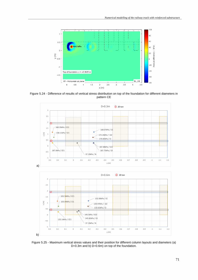
Numerical modelling of the railway track with reinforced substructure
71
Figure 5.24 - Difference of results of vertical stress distribution on top of the foundation for different diameters in pattern CE
a)
b)
Figure 5.25 - Maximum vertical stress values and their position for different column layouts and diameters (a) D=0.3m and b) D=0.6m) on top of the foundation.
168.07kPa / CC160.35kPa / CC1
187.75kPa / CE187.6kPa / CE1
170.82kPa / CI
158.11kPa / CI1
187.88kPa / EZZ
172.24kPa / IZZ
37.19kPa / N
-1
-0.5
0
0.5
1
1.5
2
2.5
3
-1.2-1.1-1-0.9-0.8-0.7-0.6-0.5-0.4-0.3-0.2-0.100.10.20.3
x (m
)
y (m)
D=0.3m 20 ton
132.06kPa / CC103.56kPa / CC1
145.82kPa / CE120.14kPa / CE1
133.62kPa / CI
103.84kPa / CI1
145.5kPa / EZZ
134.97kPa / IZZ
37.19kPa / N
-1
-0.5
0
0.5
1
1.5
2
2.5
3
-1.2-1.1-1-0.9-0.8-0.7-0.6-0.5-0.4-0.3-0.2-0.100.10.20.3
x (m
)
y (m)
D=0.6m 20 ton
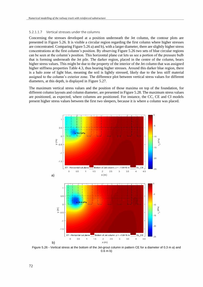
Numerical modelling of the railway track with reinforced substructure
72
5.2.1.1.7 Vertical stresses under the columns
Concerning the stresses developed at a position underneath the Jet column, the contour plots are
presented in Figure 5.26. It is visible a circular region regarding the first column where higher stresses
are concentrated. Comparing Figure 5.26 a) and b), with a larger diameter, there are slightly higher stress
concentrations at the first column’s position. By observing Figure 5.26 two sets of blue circular regions
can be seen at the column’s position. This horizontal plane cut lets us see a portion of the pressure bulb
that is forming underneath the Jet pile. The darker region, placed in the centre of the column, bears
higher stress values. This might be due to the property of the interior of the Jet column that was assigned
higher stiffness properties Table 4.3, thus bearing higher stresses. Around this darker blue region, there
is a halo zone of light blue, meaning the soil is lightly stressed, likely due to the less stiff material
assigned to the column’s exterior zone. The difference plot between vertical stress values for different
diameters, at this depth, is displayed in Figure 5.27.
The maximum vertical stress values and the position of those maxima on top of the foundation, for
different column layouts and column diameter, are presented in Figure 5.28. The maximum stress values
are positioned, as expected, where columns are positioned. For instance, the CC, CE and CI models
present higher stress values between the first two sleepers, because it is where a column was placed.
a)
b)
Figure 5.26 - Vertical stress at the bottom of the Jet-grout column in pattern CE for a diameter of 0.3 m a) and 0.6 m b)
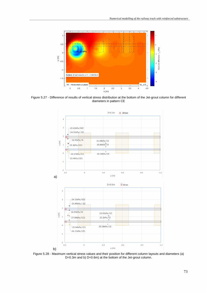
Numerical modelling of the railway track with reinforced substructure
73
Figure 5.27 - Difference of results of vertical stress distribution at the bottom of the Jet-grout column for different diameters in pattern CE
a)
b)
Figure 5.28 - Maximum vertical stress values and their position for different column layouts and diameters (a) D=0.3m and b) D=0.6m) at the bottom of the Jet-grout column.
21.68kPa / CC
25.3kPa / CC1
19.19kPa / CE
22.4kPa / CE1
20.86kPa / CI
24.37kPa / CI1
22.41kPa / EZZ
24.31kPa / IZZ
16.93kPa / N
-2
-1
0
1
2
3
4
-1.2-0.9-0.6-0.300.3
x (m
)
y (m)
D=0.3m 20 ton
23.91kPa / CC
27.99kPa / CC1
20.58kPa / CE
24.11kPa / CE1
22.2kPa / CI
25.94kPa / CI1
24.15kPa / EZZ
25.89kPa / IZZ
16.93kPa / N
-2
-1
0
1
2
3
4
-1.2-0.9-0.6-0.300.3
x (m
)
y (m)
D=0.6m 20 ton
Numerical modelling of the railway track with reinforced substructure
74
5.2.1.2 Results at the XZ plane aligned with the rail
5.2.1.2.1 Vertical rail displacements in the longitudinal alignment
The vertical rail displacements in the longitudinal alignment, for column diameters of 0.3 m and 0.6 m,
are shown in Figure 5.29 and the maximum rail displacement values are presented Table 5.1. For all
model configurations, the increase of the columns radius led to a reduction of the rail’s displacement.
As expected, the maximum displacement occurs at the position of the point load and decreases as we go
further away in the longitudinal direction. For both column diameters, between point load distance of
2.5 m and 3 m, it is observable the typical an upward vertical displacement of the rail.
To analyse the improvement in the rail displacement, the difference of results is presented in Figure
5.30. From all models, the one that showed less improvement with the increase of the column’s diameter
was the central column pattern, probably because it is the one with the least number of columns per
sleeper. Moreover, given that the position of the jet columns in this pattern is in the middle of the span
in between sleepers, the improvement obtained from the Jet-gout on the deflection does not encompass
the rail since the columns are somewhat far from it and not under the sleepers, not being able to reduce
sufficiently the rail’s displacement.
The patterns that showed better performance with the diameter’s increase were the ones where the
columns are placed closer to the rail such as the models CE or CI. The pattern that showed the most
improvement by increasing the radius of the column was model CEZZ. As mentioned earlier, by
increasing the column’s diameter, part of it envelops the surface under the sleepers adjacent to it. This
creates a larger support to the sleepers, reducing deflections under it. By implementing a zig-zag pattern
and diameter increase, the sleepers support will be improved from both of its edges as explained in
Figure 5.31.
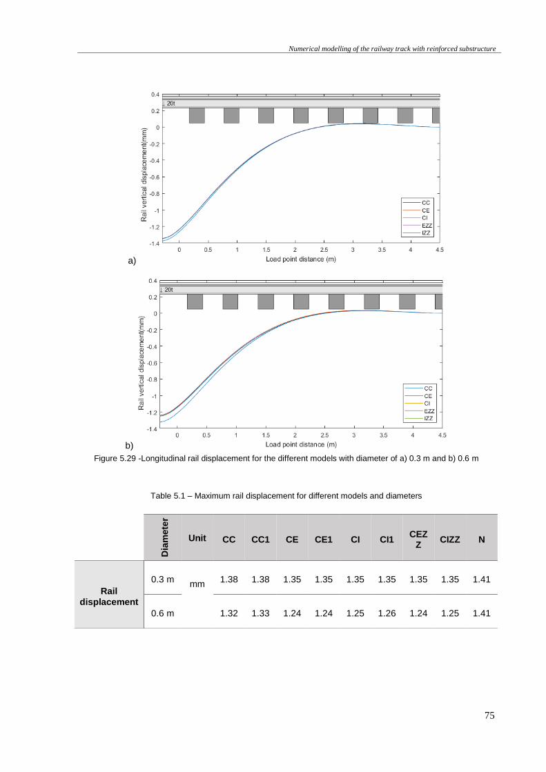
Numerical modelling of the railway track with reinforced substructure
75
a)
b)
Figure 5.29 -Longitudinal rail displacement for the different models with diameter of a) 0.3 m and b) 0.6 m
Table 5.1 – Maximum rail displacement for different models and diameters
Dia
me
ter
Unit CC CC1 CE CE1 CI CI1 CEZ
Z CIZZ N
Rail
displacement
0.3 m
mm 1.38 1.38 1.35 1.35 1.35 1.35 1.35 1.35 1.41
0.6 m 1.32 1.33 1.24 1.24 1.25 1.26 1.24 1.25 1.41
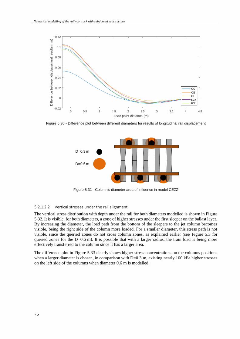
Numerical modelling of the railway track with reinforced substructure
76
Figure 5.30 - Difference plot between different diameters for results of longitudinal rail displacement
Figure 5.31 - Column's diameter area of influence in model CEZZ
5.2.1.2.2 Vertical stresses under the rail alignment
The vertical stress distribution with depth under the rail for both diameters modelled is shown in Figure
5.32. It is visible, for both diameters, a zone of higher stresses under the first sleeper on the ballast layer.
By increasing the diameter, the load path from the bottom of the sleepers to the jet column becomes
visible, being the right side of the column more loaded. For a smaller diameter, this stress path is not
visible, since the queried zones do not cross column zones, as explained earlier (see Figure 5.3 for
queried zones for the D=0.6 m). It is possible that with a larger radius, the train load is being more
effectively transferred to the column since it has a larger area.
The difference plot in Figure 5.33 clearly shows higher stress concentrations on the columns positions
when a larger diameter is chosen, in comparison with D=0.3 m, existing nearly 100 kPa higher stresses
on the left side of the columns when diameter 0.6 m is modelled.
D=0.3 m
D=0.6 m
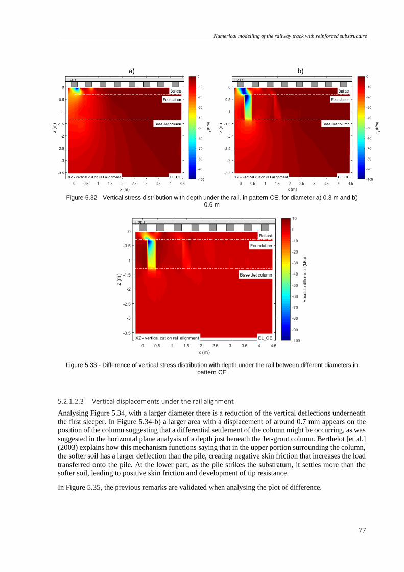
Numerical modelling of the railway track with reinforced substructure
77
a)
b)
Figure 5.32 - Vertical stress distribution with depth under the rail, in pattern CE, for diameter a) 0.3 m and b)
0.6 m
Figure 5.33 - Difference of vertical stress distribution with depth under the rail between different diameters in pattern CE
5.2.1.2.3 Vertical displacements under the rail alignment
Analysing Figure 5.34, with a larger diameter there is a reduction of the vertical deflections underneath
the first sleeper. In Figure 5.34-b) a larger area with a displacement of around 0.7 mm appears on the
position of the column suggesting that a differential settlement of the column might be occurring, as was
suggested in the horizontal plane analysis of a depth just beneath the Jet-grout column. Berthelot [et al.]
(2003) explains how this mechanism functions saying that in the upper portion surrounding the column,
the softer soil has a larger deflection than the pile, creating negative skin friction that increases the load
transferred onto the pile. At the lower part, as the pile strikes the substratum, it settles more than the
softer soil, leading to positive skin friction and development of tip resistance.
In Figure 5.35, the previous remarks are validated when analysing the plot of difference.
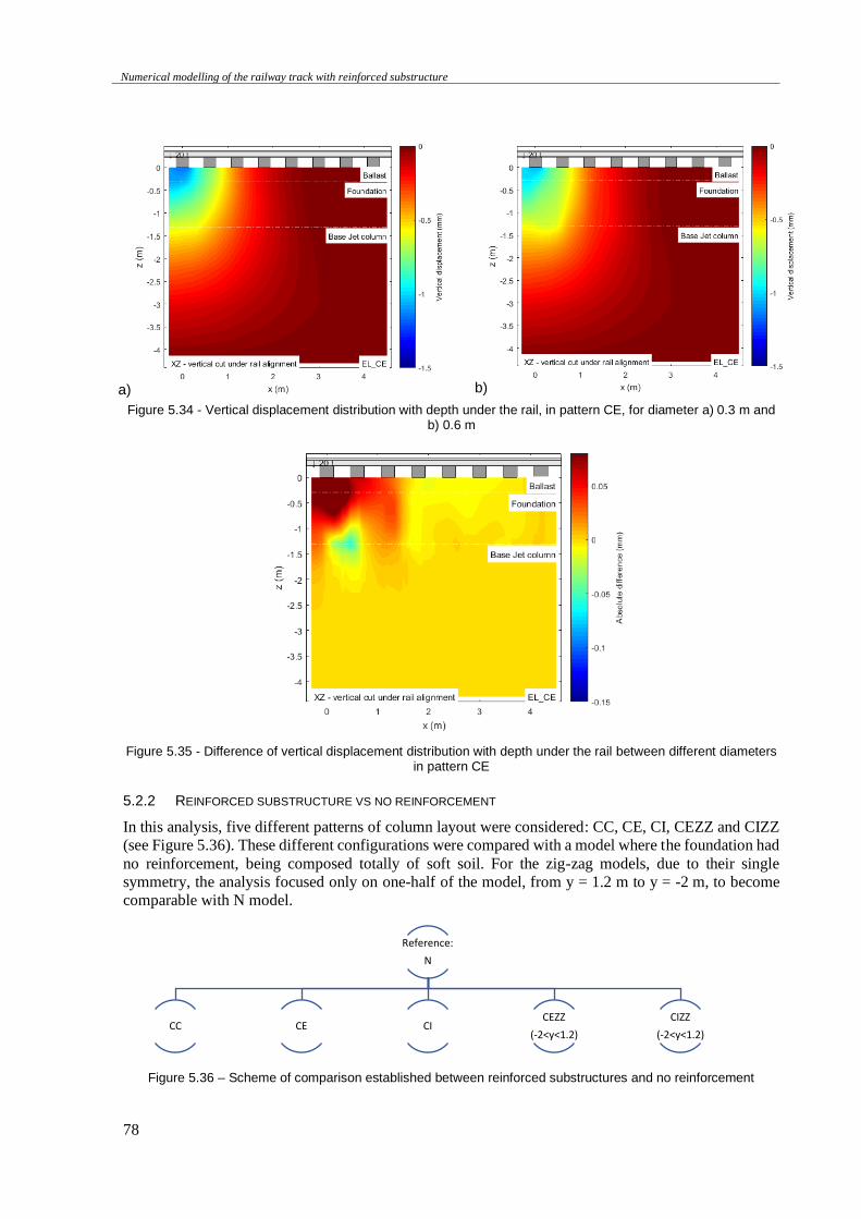
Numerical modelling of the railway track with reinforced substructure
78
a) b)
Figure 5.34 - Vertical displacement distribution with depth under the rail, in pattern CE, for diameter a) 0.3 m and b) 0.6 m
Figure 5.35 - Difference of vertical displacement distribution with depth under the rail between different diameters in pattern CE
5.2.2 REINFORCED SUBSTRUCTURE VS NO REINFORCEMENT
In this analysis, five different patterns of column layout were considered: CC, CE, CI, CEZZ and CIZZ
(see Figure 5.36). These different configurations were compared with a model where the foundation had
no reinforcement, being composed totally of soft soil. For the zig-zag models, due to their single
symmetry, the analysis focused only on one-half of the model, from y = 1.2 m to y = -2 m, to become
comparable with N model.
Figure 5.36 – Scheme of comparison established between reinforced substructures and no reinforcement
Reference:
N
CC CE CICEZZ
(-2<y<1.2)
CIZZ
(-2<y<1.2)
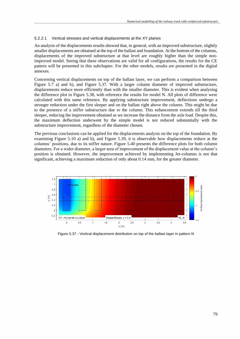
Numerical modelling of the railway track with reinforced substructure
79
5.2.2.1 Vertical stresses and vertical displacements at the XY planes
An analysis of the displacements results showed that, in general, with an improved substructure, slightly
smaller displacements are obtained at the top of the ballast and foundation. At the bottom of the columns,
displacements of the improved substructure at that level are roughly higher than the simple non-
improved model. Seeing that these observations are valid for all configurations, the results for the CE
pattern will be presented in this subchapter. For the other models, results are presented in the digital
annexes.
Concerning vertical displacements on top of the ballast layer, we can perform a comparison between
Figure 5.7 a) and b), and Figure 5.37. With a larger column diameter of improved substructure,
displacements reduce more efficiently than with the smaller diameter. This is evident when analysing
the difference plot in Figure 5.38, with reference the results for model N. All plots of difference were
calculated with this same reference. By applying substructure improvement, deflections undergo a
stronger reduction under the first sleeper and on the ballast right above the column. This might be due
to the presence of a stiffer substructure due to the column. This enhancement extends till the third
sleeper, reducing the improvement obtained as we increase the distance from the axle load. Despite this,
the maximum deflection underwent by the simple model is not reduced substantially with the
substructure improvement, regardless of the diameter chosen.
The previous conclusions can be applied for the displacements analysis on the top of the foundation. By
examining Figure 5.10 a) and b), and Figure 5.39, it is observable how displacements reduce at the
columns’ positions, due to its stiffer nature. Figure 5.40 presents the difference plots for both column
diameters. For a wider diameter, a larger area of improvement of the displacement value at the column’s
position is obtained. However, the improvement achieved by implementing Jet-columns is not that
significant, achieving a maximum reduction of only about 0.14 mm, for the greater diameter.
Figure 5.37 - Vertical displacement distribution on top of the ballast layer in pattern N
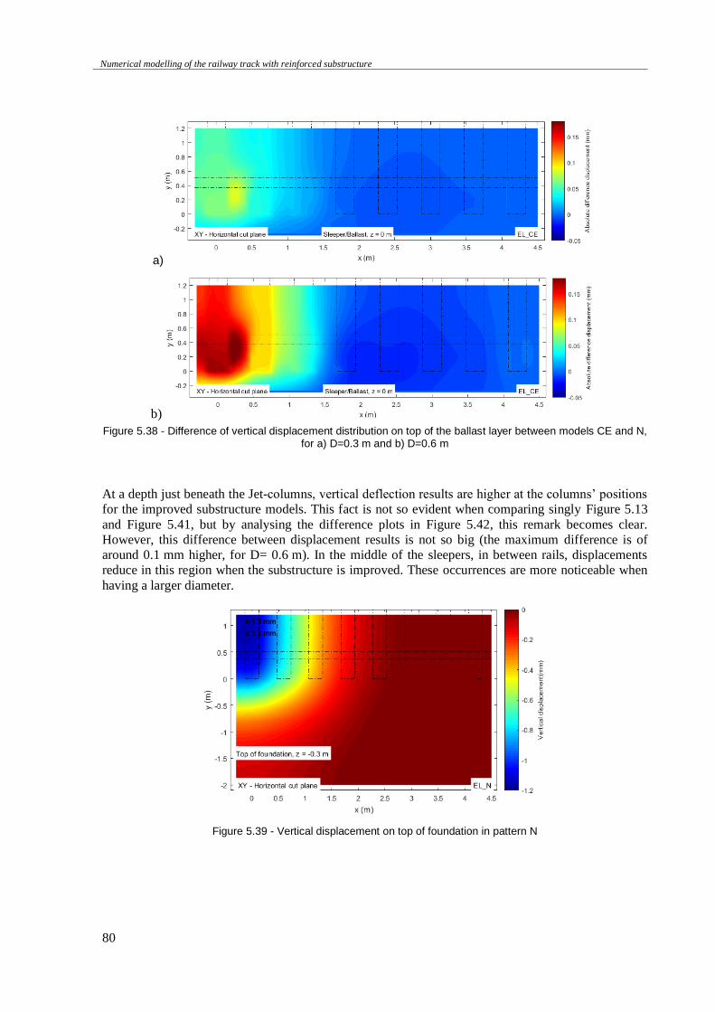
Numerical modelling of the railway track with reinforced substructure
80
a)
b)
Figure 5.38 - Difference of vertical displacement distribution on top of the ballast layer between models CE and N, for a) D=0.3 m and b) D=0.6 m
At a depth just beneath the Jet-columns, vertical deflection results are higher at the columns’ positions
for the improved substructure models. This fact is not so evident when comparing singly Figure 5.13
and Figure 5.41, but by analysing the difference plots in Figure 5.42, this remark becomes clear.
However, this difference between displacement results is not so big (the maximum difference is of
around 0.1 mm higher, for D= 0.6 m). In the middle of the sleepers, in between rails, displacements
reduce in this region when the substructure is improved. These occurrences are more noticeable when
having a larger diameter.
Figure 5.39 - Vertical displacement on top of foundation in pattern N
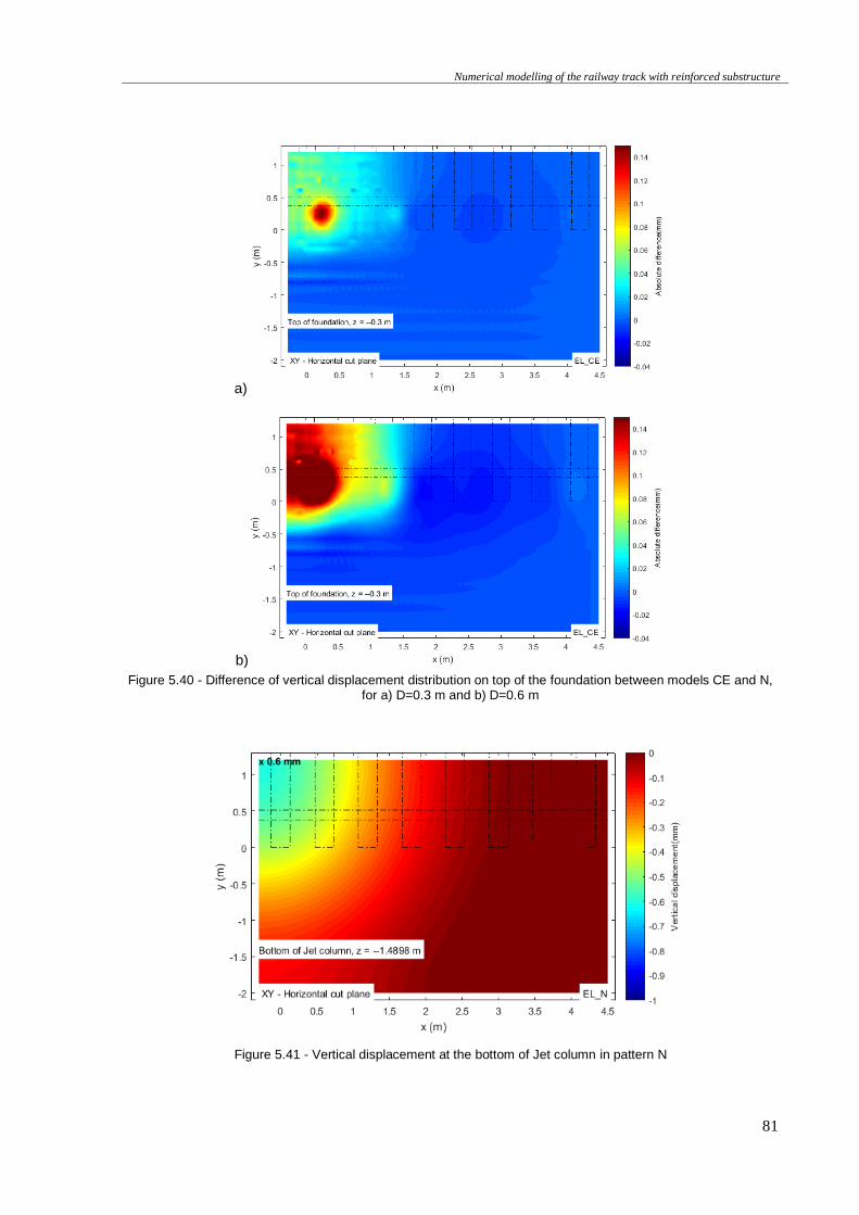
Numerical modelling of the railway track with reinforced substructure
81
a)
b)
Figure 5.40 - Difference of vertical displacement distribution on top of the foundation between models CE and N, for a) D=0.3 m and b) D=0.6 m
Figure 5.41 - Vertical displacement at the bottom of Jet column in pattern N
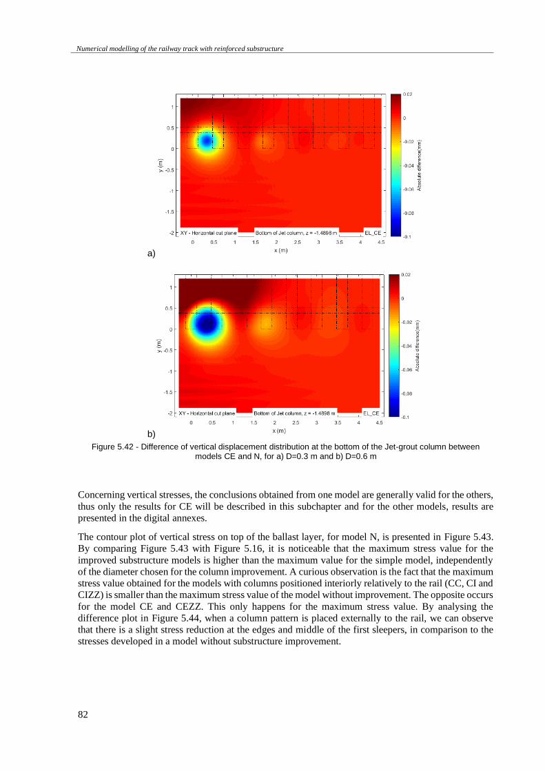
Numerical modelling of the railway track with reinforced substructure
82
a)
b)
Figure 5.42 - Difference of vertical displacement distribution at the bottom of the Jet-grout column between models CE and N, for a) D=0.3 m and b) D=0.6 m
Concerning vertical stresses, the conclusions obtained from one model are generally valid for the others,
thus only the results for CE will be described in this subchapter and for the other models, results are
presented in the digital annexes.
The contour plot of vertical stress on top of the ballast layer, for model N, is presented in Figure 5.43.
By comparing Figure 5.43 with Figure 5.16, it is noticeable that the maximum stress value for the
improved substructure models is higher than the maximum value for the simple model, independently
of the diameter chosen for the column improvement. A curious observation is the fact that the maximum
stress value obtained for the models with columns positioned interiorly relatively to the rail (CC, CI and
CIZZ) is smaller than the maximum stress value of the model without improvement. The opposite occurs
for the model CE and CEZZ. This only happens for the maximum stress value. By analysing the
difference plot in Figure 5.44, when a column pattern is placed externally to the rail, we can observe
that there is a slight stress reduction at the edges and middle of the first sleepers, in comparison to the
stresses developed in a model without substructure improvement.
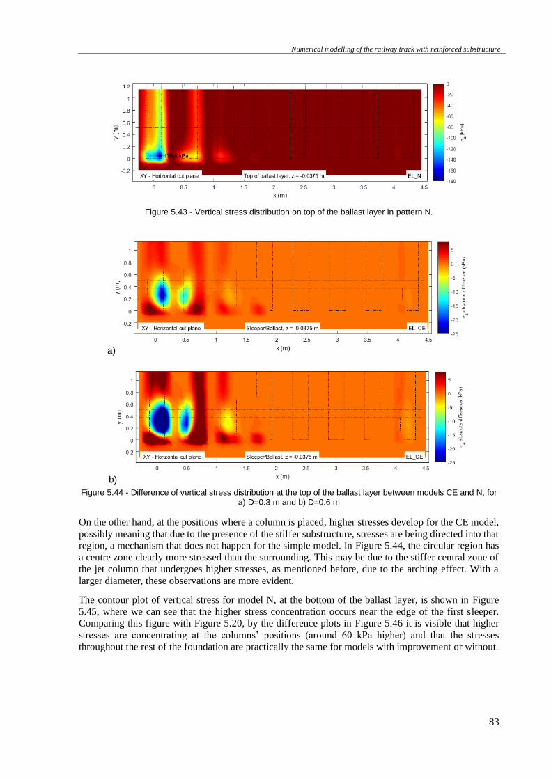
Numerical modelling of the railway track with reinforced substructure
83
Figure 5.43 - Vertical stress distribution on top of the ballast layer in pattern N.
a)
b)
Figure 5.44 - Difference of vertical stress distribution at the top of the ballast layer between models CE and N, for a) D=0.3 m and b) D=0.6 m
On the other hand, at the positions where a column is placed, higher stresses develop for the CE model,
possibly meaning that due to the presence of the stiffer substructure, stresses are being directed into that
region, a mechanism that does not happen for the simple model. In Figure 5.44, the circular region has
a centre zone clearly more stressed than the surrounding. This may be due to the stiffer central zone of
the jet column that undergoes higher stresses, as mentioned before, due to the arching effect. With a
larger diameter, these observations are more evident.
The contour plot of vertical stress for model N, at the bottom of the ballast layer, is shown in Figure
5.45, where we can see that the higher stress concentration occurs near the edge of the first sleeper.
Comparing this figure with Figure 5.20, by the difference plots in Figure 5.46 it is visible that higher
stresses are concentrating at the columns’ positions (around 60 kPa higher) and that the stresses
throughout the rest of the foundation are practically the same for models with improvement or without.
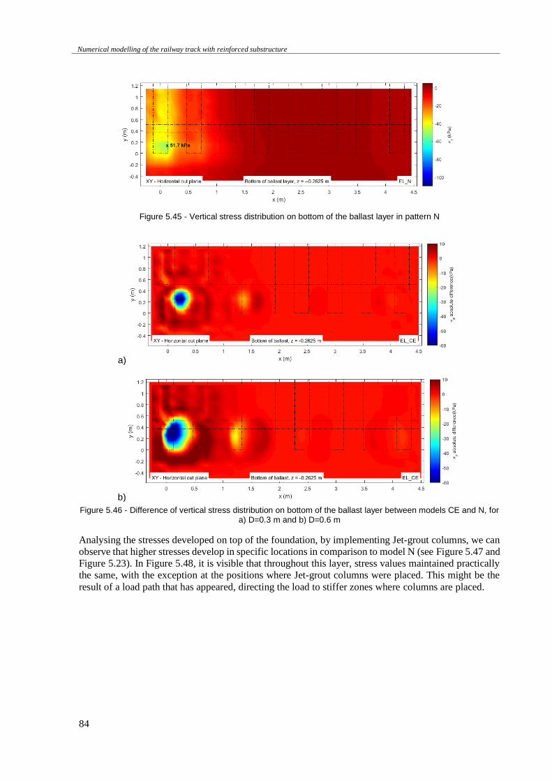
Numerical modelling of the railway track with reinforced substructure
84
Figure 5.45 - Vertical stress distribution on bottom of the ballast layer in pattern N
a)
b)
Figure 5.46 - Difference of vertical stress distribution on bottom of the ballast layer between models CE and N, for a) D=0.3 m and b) D=0.6 m
Analysing the stresses developed on top of the foundation, by implementing Jet-grout columns, we can
observe that higher stresses develop in specific locations in comparison to model N (see Figure 5.47 and
Figure 5.23). In Figure 5.48, it is visible that throughout this layer, stress values maintained practically
the same, with the exception at the positions where Jet-grout columns were placed. This might be the
result of a load path that has appeared, directing the load to stiffer zones where columns are placed.
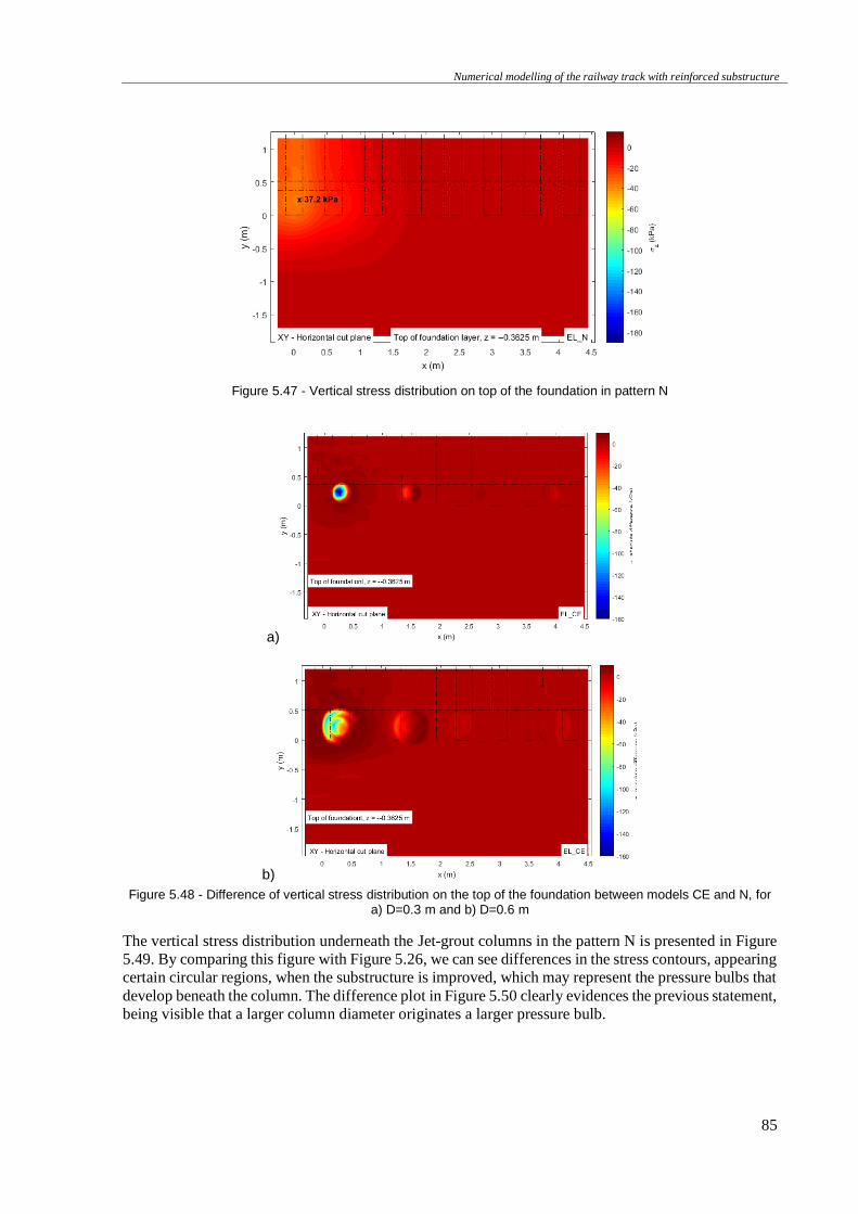
Numerical modelling of the railway track with reinforced substructure
85
Figure 5.47 - Vertical stress distribution on top of the foundation in pattern N
a)
b)
Figure 5.48 - Difference of vertical stress distribution on the top of the foundation between models CE and N, for a) D=0.3 m and b) D=0.6 m
The vertical stress distribution underneath the Jet-grout columns in the pattern N is presented in Figure
5.49. By comparing this figure with Figure 5.26, we can see differences in the stress contours, appearing
certain circular regions, when the substructure is improved, which may represent the pressure bulbs that
develop beneath the column. The difference plot in Figure 5.50 clearly evidences the previous statement,
being visible that a larger column diameter originates a larger pressure bulb.
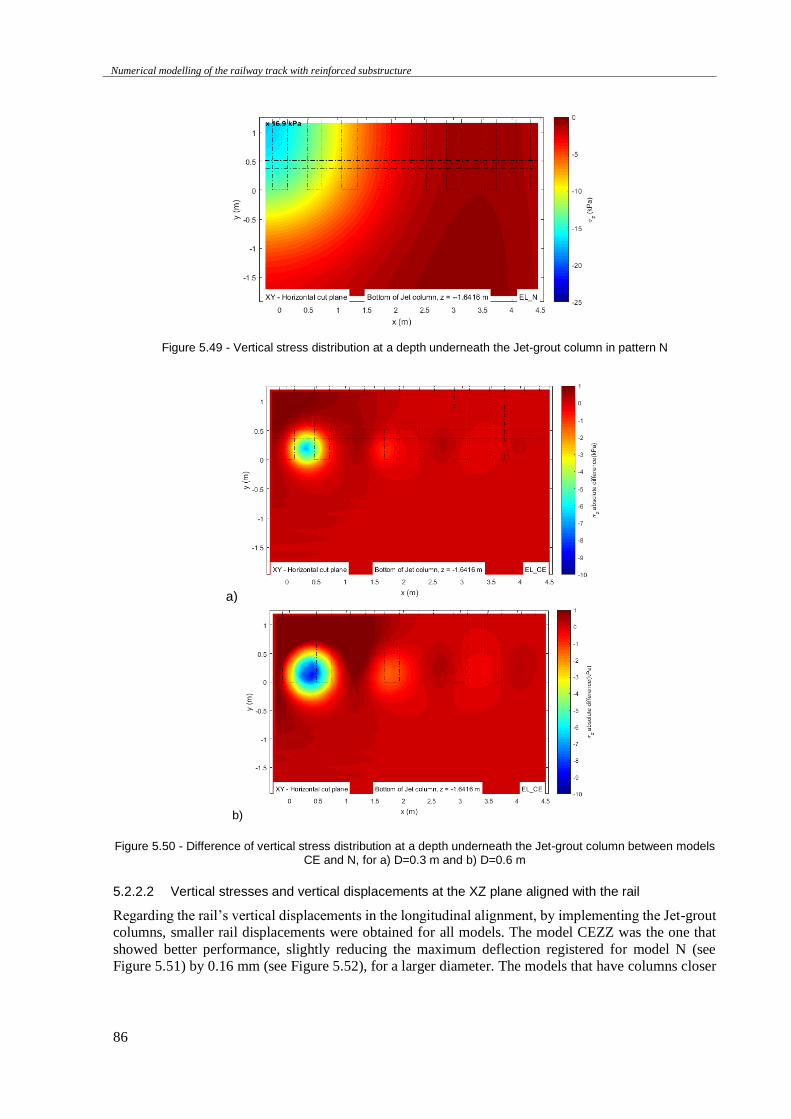
Numerical modelling of the railway track with reinforced substructure
86
Figure 5.49 - Vertical stress distribution at a depth underneath the Jet-grout column in pattern N
a)
b)
Figure 5.50 - Difference of vertical stress distribution at a depth underneath the Jet-grout column between models CE and N, for a) D=0.3 m and b) D=0.6 m
5.2.2.2 Vertical stresses and vertical displacements at the XZ plane aligned with the rail
Regarding the rail’s vertical displacements in the longitudinal alignment, by implementing the Jet-grout
columns, smaller rail displacements were obtained for all models. The model CEZZ was the one that
showed better performance, slightly reducing the maximum deflection registered for model N (see
Figure 5.51) by 0.16 mm (see Figure 5.52), for a larger diameter. The models that have columns closer
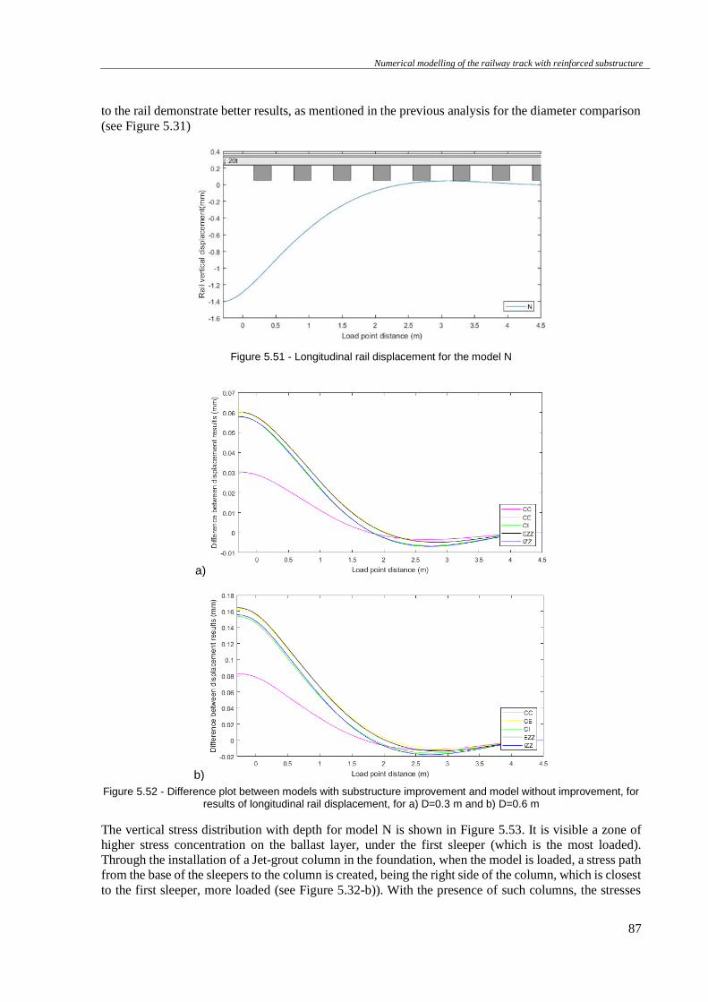
Numerical modelling of the railway track with reinforced substructure
87
to the rail demonstrate better results, as mentioned in the previous analysis for the diameter comparison
(see Figure 5.31)
Figure 5.51 - Longitudinal rail displacement for the model N
a)
b)
Figure 5.52 - Difference plot between models with substructure improvement and model without improvement, for results of longitudinal rail displacement, for a) D=0.3 m and b) D=0.6 m
The vertical stress distribution with depth for model N is shown in Figure 5.53. It is visible a zone of
higher stress concentration on the ballast layer, under the first sleeper (which is the most loaded).
Through the installation of a Jet-grout column in the foundation, when the model is loaded, a stress path
from the base of the sleepers to the column is created, being the right side of the column, which is closest
to the first sleeper, more loaded (see Figure 5.32-b)). With the presence of such columns, the stresses
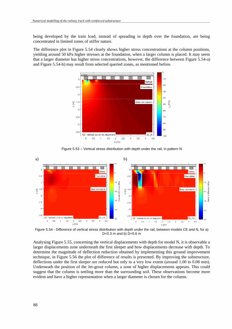
Numerical modelling of the railway track with reinforced substructure
88
being developed by the train load, instead of spreading in depth over the foundation, are being
concentrated in limited zones of stiffer nature.
The difference plot in Figure 5.54 clearly shows higher stress concentrations at the column positions,
yielding around 50 kPa higher stresses at the foundation, when a larger column is placed. It may seem
that a larger diameter has higher stress concentrations, however, the difference between Figure 5.54-a)
and Figure 5.54-b) may result from selected queried zones, as mentioned before.
Figure 5.53 – Vertical stress distribution with depth under the rail, in pattern N
a)
b)
Figure 5.54 - Difference of vertical stress distribution with depth under the rail, between models CE and N, for a)
D=0.3 m and b) D=0.6 m
Analysing Figure 5.55, concerning the vertical displacements with depth for model N, it is observable a
larger displacements zone underneath the first sleeper and how displacements decrease with depth. To
determine the magnitude of deflection reduction obtained by implementing this ground improvement
technique, in Figure 5.56 the plot of difference of results is presented. By improving the substructure,
deflections under the first sleeper are reduced but only to a very low extent (around 1.00 to 0.08 mm).
Underneath the position of the Jet-grout column, a zone of higher displacements appears. This could
suggest that the column is settling more than the surrounding soil. These observations become more
evident and have a higher representation when a larger diameter is chosen for the column.
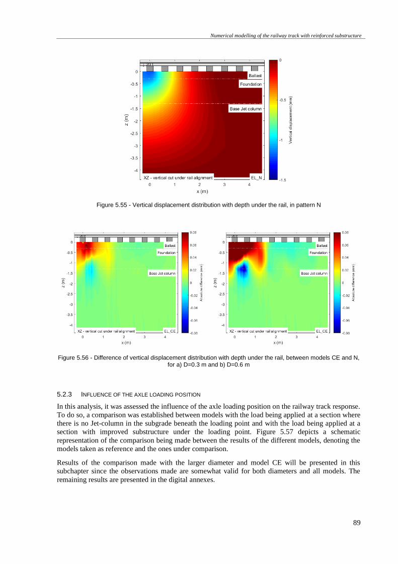
Numerical modelling of the railway track with reinforced substructure
89
Figure 5.55 - Vertical displacement distribution with depth under the rail, in pattern N
Figure 5.56 - Difference of vertical displacement distribution with depth under the rail, between models CE and N, for a) D=0.3 m and b) D=0.6 m
5.2.3 INFLUENCE OF THE AXLE LOADING POSITION
In this analysis, it was assessed the influence of the axle loading position on the railway track response.
To do so, a comparison was established between models with the load being applied at a section where
there is no Jet-column in the subgrade beneath the loading point and with the load being applied at a
section with improved substructure under the loading point. Figure 5.57 depicts a schematic
representation of the comparison being made between the results of the different models, denoting the
models taken as reference and the ones under comparison.
Results of the comparison made with the larger diameter and model CE will be presented in this
subchapter since the observations made are somewhat valid for both diameters and all models. The
remaining results are presented in the digital annexes.
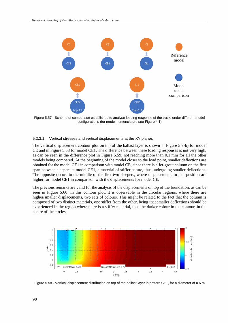
Numerical modelling of the railway track with reinforced substructure
90
Reference
model
Model
under
comparison
Figure 5.57 - Scheme of comparison established to analyse loading response of the track, under different model
configurations (for model nomenclature see Figure 4.1)
5.2.3.1 Vertical stresses and vertical displacements at the XY planes
The vertical displacement contour plot on top of the ballast layer is shown in Figure 5.7-b) for model
CE and in Figure 5.58 for model CE1. The difference between these loading responses is not very high,
as can be seen in the difference plot in Figure 5.59, not reaching more than 0.1 mm for all the other
models being compared. At the beginning of the model closer to the load point, smaller deflections are
obtained for the model CE1 in comparison with model CE, since there is a Jet-grout column on the first
span between sleepers at model CE1, a material of stiffer nature, thus undergoing smaller deflections.
The opposite occurs in the middle of the first two sleepers, where displacements in that position are
higher for model CE1 in comparison with the displacements for model CE.
The previous remarks are valid for the analysis of the displacements on top of the foundation, as can be
seen in Figure 5.60. In this contour plot, it is observable in the circular regions, where there are
higher/smaller displacements, two sets of colours. This might be related to the fact that the column is
composed of two distinct materials, one stiffer from the other, being that smaller deflections should be
experienced in the region where there is a stiffer material, thus the darker colour in the contour, in the
centre of the circles.
Figure 5.58 - Vertical displacement distribution on top of the ballast layer in pattern CE1, for a diameter of 0.6 m
CC1
CC
CE1
CE
CI1
CI
CEZZ
-2<y<1.2
CE1
CIZZ
-2<y<1.2
CI1
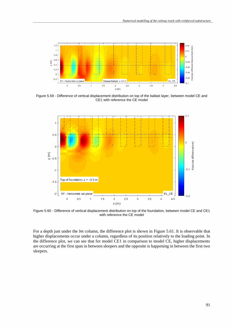
Numerical modelling of the railway track with reinforced substructure
91
Figure 5.59 - Difference of vertical displacement distribution on top of the ballast layer, between model CE and CE1 with reference the CE model
Figure 5.60 - Difference of vertical displacement distribution on top of the foundation, between model CE and CE1 with reference the CE model
For a depth just under the Jet column, the difference plot is shown in Figure 5.61. It is observable that
higher displacements occur under a column, regardless of its position relatively to the loading point. In
the difference plot, we can see that for model CE1 in comparison to model CE, higher displacements
are occurring at the first span in between sleepers and the opposite is happening in between the first two
sleepers.

Numerical modelling of the railway track with reinforced substructure
92
Figure 5.61 - Difference of vertical displacement distribution at a depth slightly under the Jet-grout column, between model CE and CE1 with reference the CE model
Regarding the vertical stress developed at the level of ballast layer, foundation and beneath the jet
column, the following observations, regarding the contour plots, are valid for all levels. The contour
plots of vertical stresses on top and bottom of the ballast layer, on top of the foundation and beneath the
Jet-grout column, for model CE1, are presented in Figure 5.62. The corresponding plots of differences
are shown in Figure 5.63.
In the difference plot, it is visible that higher stresses develop at the beginning of the model, at x= -
0.3 m, for the model CE1, due to the presence of a column in this position. This stress concentration
happens whenever there is a column, despite the model considered. The presence of a column may lead
to a higher stress concentration, due to a loading path of stress transference to stiffer zones that is
possibly being created. The opposite is occurring for model CE, in comparison to model CE1, where we
can see stress concentrations in the middle of the first two sleepers, once more, at the column’s position.
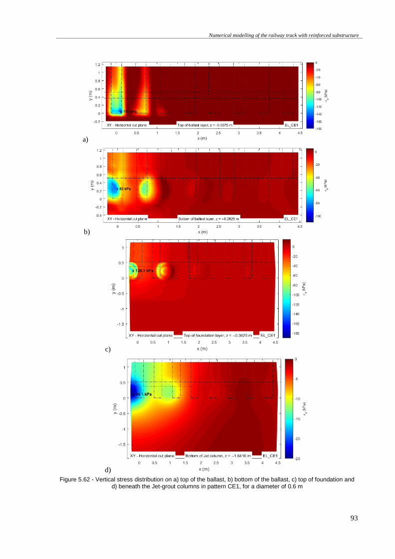
Numerical modelling of the railway track with reinforced substructure
93
a)
b)
c)
d)
Figure 5.62 - Vertical stress distribution on a) top of the ballast, b) bottom of the ballast, c) top of foundation and d) beneath the Jet-grout columns in pattern CE1, for a diameter of 0.6 m
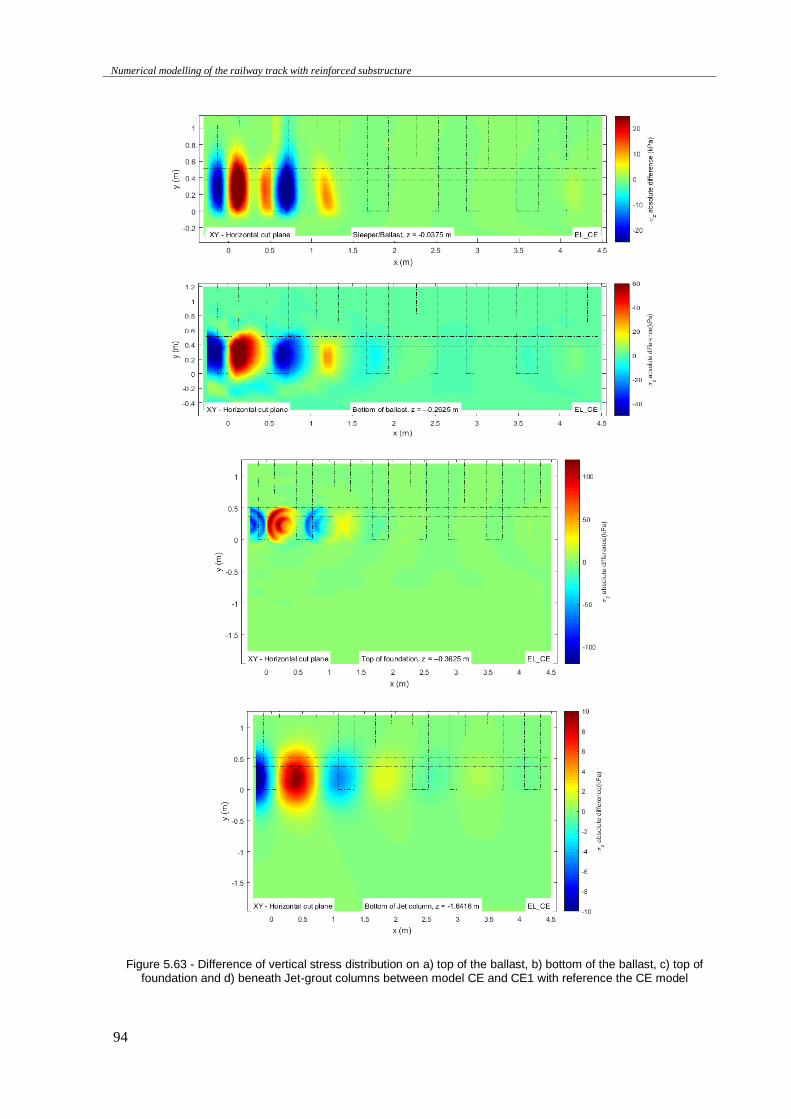
Numerical modelling of the railway track with reinforced substructure
94
Figure 5.63 - Difference of vertical stress distribution on a) top of the ballast, b) bottom of the ballast, c) top of foundation and d) beneath Jet-grout columns between model CE and CE1 with reference the CE model
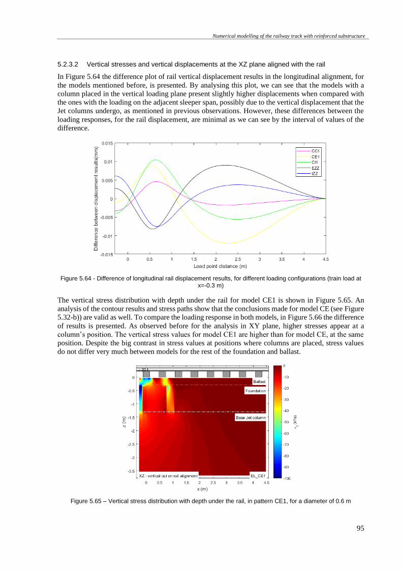
Numerical modelling of the railway track with reinforced substructure
95
5.2.3.2 Vertical stresses and vertical displacements at the XZ plane aligned with the rail
In Figure 5.64 the difference plot of rail vertical displacement results in the longitudinal alignment, for
the models mentioned before, is presented. By analysing this plot, we can see that the models with a
column placed in the vertical loading plane present slightly higher displacements when compared with
the ones with the loading on the adjacent sleeper span, possibly due to the vertical displacement that the
Jet columns undergo, as mentioned in previous observations. However, these differences between the
loading responses, for the rail displacement, are minimal as we can see by the interval of values of the
difference.
Figure 5.64 - Difference of longitudinal rail displacement results, for different loading configurations (train load at x=-0.3 m)
The vertical stress distribution with depth under the rail for model CE1 is shown in Figure 5.65. An
analysis of the contour results and stress paths show that the conclusions made for model CE (see Figure
5.32-b)) are valid as well. To compare the loading response in both models, in Figure 5.66 the difference
of results is presented. As observed before for the analysis in XY plane, higher stresses appear at a
column’s position. The vertical stress values for model CE1 are higher than for model CE, at the same
position. Despite the big contrast in stress values at positions where columns are placed, stress values
do not differ very much between models for the rest of the foundation and ballast.
Figure 5.65 – Vertical stress distribution with depth under the rail, in pattern CE1, for a diameter of 0.6 m
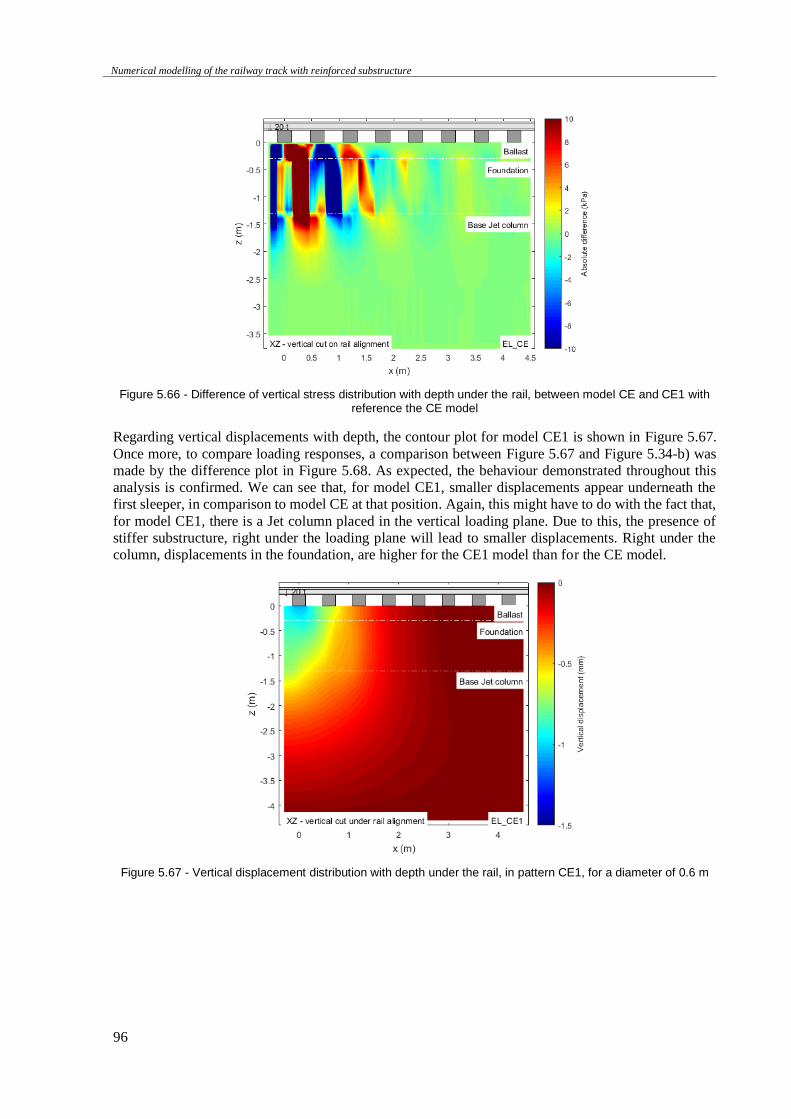
Numerical modelling of the railway track with reinforced substructure
96
Figure 5.66 - Difference of vertical stress distribution with depth under the rail, between model CE and CE1 with reference the CE model
Regarding vertical displacements with depth, the contour plot for model CE1 is shown in Figure 5.67.
Once more, to compare loading responses, a comparison between Figure 5.67 and Figure 5.34-b) was
made by the difference plot in Figure 5.68. As expected, the behaviour demonstrated throughout this
analysis is confirmed. We can see that, for model CE1, smaller displacements appear underneath the
first sleeper, in comparison to model CE at that position. Again, this might have to do with the fact that,
for model CE1, there is a Jet column placed in the vertical loading plane. Due to this, the presence of
stiffer substructure, right under the loading plane will lead to smaller displacements. Right under the
column, displacements in the foundation, are higher for the CE1 model than for the CE model.
Figure 5.67 - Vertical displacement distribution with depth under the rail, in pattern CE1, for a diameter of 0.6 m
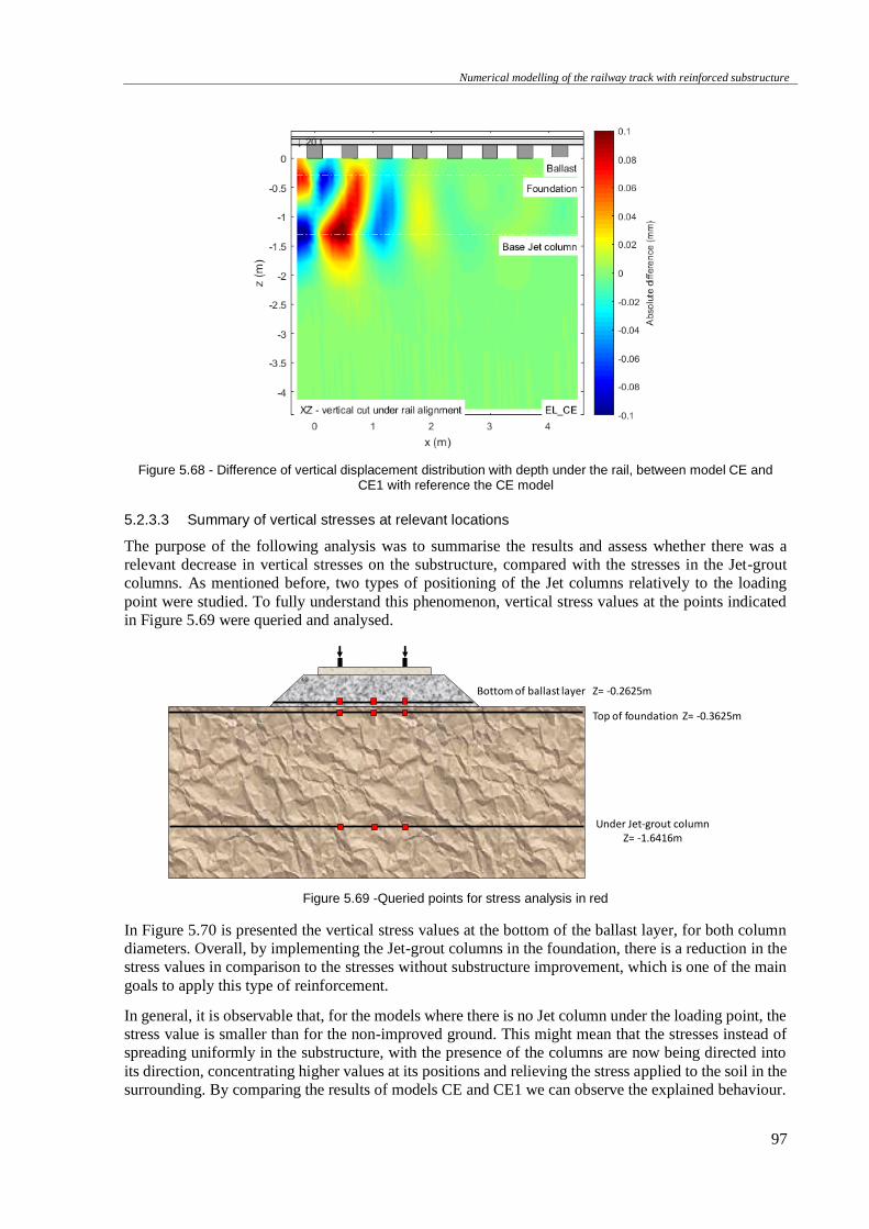
Numerical modelling of the railway track with reinforced substructure
97
Figure 5.68 - Difference of vertical displacement distribution with depth under the rail, between model CE and CE1 with reference the CE model
5.2.3.3 Summary of vertical stresses at relevant locations
The purpose of the following analysis was to summarise the results and assess whether there was a
relevant decrease in vertical stresses on the substructure, compared with the stresses in the Jet-grout
columns. As mentioned before, two types of positioning of the Jet columns relatively to the loading
point were studied. To fully understand this phenomenon, vertical stress values at the points indicated
in Figure 5.69 were queried and analysed.
Figure 5.69 -Queried points for stress analysis in red
In Figure 5.70 is presented the vertical stress values at the bottom of the ballast layer, for both column
diameters. Overall, by implementing the Jet-grout columns in the foundation, there is a reduction in the
stress values in comparison to the stresses without substructure improvement, which is one of the main
goals to apply this type of reinforcement.
In general, it is observable that, for the models where there is no Jet column under the loading point, the
stress value is smaller than for the non-improved ground. This might mean that the stresses instead of
spreading uniformly in the substructure, with the presence of the columns are now being directed into
its direction, concentrating higher values at its positions and relieving the stress applied to the soil in the
surrounding. By comparing the results of models CE and CE1 we can observe the explained behaviour.
Top of foundation Z= -0.3625m
Bottom of ballast layer Z= -0.2625m
Under Jet-grout columnZ= -1.6416m
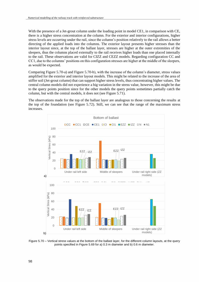
Numerical modelling of the railway track with reinforced substructure
98
With the presence of a Jet-grout column under the loading point in model CE1, in comparison with CE,
there is a higher stress concentration at the column. For the exterior and interior configurations, higher
stress levels are occurring under the rail, since the column’s position relatively to the rail allows a better
directing of the applied loads into the columns. The exterior layout presents higher stresses than the
interior layout since, at the top of the ballast layer, stresses are higher at the outer extremities of the
sleepers, thus the columns placed externally to the rail receives higher loads than one placed internally
to the rail. These observations are valid for CIZZ and CEZZ models. Regarding configuration CC and
CC1, due to the columns’ positions on this configuration stresses are higher at the middle of the sleepers,
as would be expected.
Comparing Figure 5.70-a) and Figure 5.70-b), with the increase of the column’s diameter, stress values
amplified for the exterior and interior layout models. This might be related to the increase of the area of
stiffer soil (Jet-grout column) that can support higher stress levels, thus concentrating higher values. The
central column models did not experience a big variation in the stress value, however, this might be due
to the query points position since for the other models the query points sometimes partially catch the
column, but with the central models, it does not (see Figure 5.71).
The observations made for the top of the ballast layer are analogous to those concerning the results at
the top of the foundation (see Figure 5.72). Still, we can see that the range of the maximum stress
increases.
a)
b)
Figure 5.70 – Vertical stress values at the bottom of the ballast layer, for the different column layouts, at the query points specified in Figure 5.69 for a) 0.3 m diameter and b) 0.6 m diameter.
EZZ EZZIZZIZZ
0
20
40
60
80
100
Under rail left side Middle of sleepers Under rail right side (ZZmodels)
Ve
rtic
al S
tre
s (
kP
a)
Bottom of ballast
CC CC1 CE CE1 CI CI1 EZZ IZZ N N1
EZZ EZZIZZ
IZZ
0
20
40
60
80
100
Under rail left side Middle of sleepers Under rail right side (ZZmodels)
Ve
rtic
al S
tre
s (
kP
a)
Bottom of ballast
CC CC1 CE CE1 CI CI1 EZZ IZZ N N1
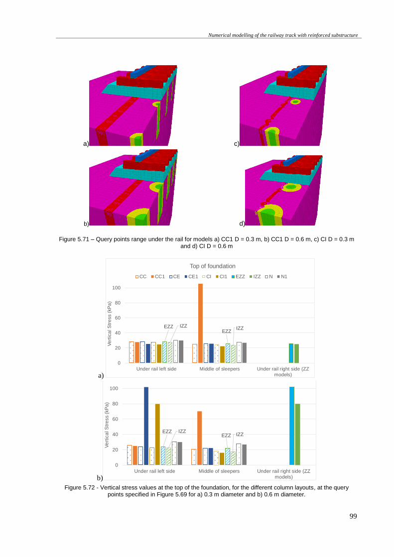
Numerical modelling of the railway track with reinforced substructure
99
a) c)
b) d)
Figure 5.71 – Query points range under the rail for models a) CC1 D = 0.3 m, b) CC1 D = 0.6 m, c) CI D = 0.3 m and d) CI D = 0.6 m
a)
b)
Figure 5.72 - Vertical stress values at the top of the foundation, for the different column layouts, at the query points specified in Figure 5.69 for a) 0.3 m diameter and b) 0.6 m diameter.
EZZEZZ
IZZ IZZ
0
20
40
60
80
100
Under rail left side Middle of sleepers Under rail right side (ZZmodels)
Ve
rtic
al S
tre
ss (
kP
a)
Top of foundation
CC CC1 CE CE1 CI CI1 EZZ IZZ N N1
EZZEZZ
IZZIZZ
0
20
40
60
80
100
Under rail left side Middle of sleepers Under rail right side (ZZmodels)
Ve
rtic
al S
tre
ss (
kP
a)
Top of foundation
CC CC1 CE CE1 CI CI1 EZZ IZZ N N1
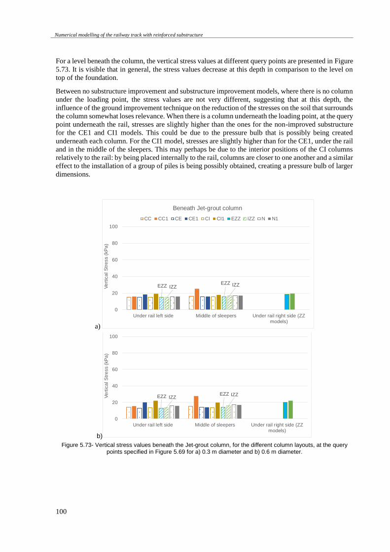
Numerical modelling of the railway track with reinforced substructure
100
For a level beneath the column, the vertical stress values at different query points are presented in Figure
5.73. It is visible that in general, the stress values decrease at this depth in comparison to the level on
top of the foundation.
Between no substructure improvement and substructure improvement models, where there is no column
under the loading point, the stress values are not very different, suggesting that at this depth, the
influence of the ground improvement technique on the reduction of the stresses on the soil that surrounds
the column somewhat loses relevance. When there is a column underneath the loading point, at the query
point underneath the rail, stresses are slightly higher than the ones for the non-improved substructure
for the CE1 and CI1 models. This could be due to the pressure bulb that is possibly being created
underneath each column. For the CI1 model, stresses are slightly higher than for the CE1, under the rail
and in the middle of the sleepers. This may perhaps be due to the interior positions of the CI columns
relatively to the rail: by being placed internally to the rail, columns are closer to one another and a similar
effect to the installation of a group of piles is being possibly obtained, creating a pressure bulb of larger
dimensions.
a)
b)
Figure 5.73- Vertical stress values beneath the Jet-grout column, for the different column layouts, at the query points specified in Figure 5.69 for a) 0.3 m diameter and b) 0.6 m diameter.
EZZEZZ
IZZ IZZ
0
20
40
60
80
100
Under rail left side Middle of sleepers Under rail right side (ZZmodels)
Ve
rtic
al S
tre
ss (
kP
a)
Beneath Jet-grout column
CC CC1 CE CE1 CI CI1 EZZ IZZ N N1
EZZEZZ
IZZIZZ
0
20
40
60
80
100
Under rail left side Middle of sleepers Under rail right side (ZZmodels)
Ve
rtic
al S
tre
ss (
kP
a)
Beneath Jet-grout column
CC CC1 CE CE1 CI CI1 EZZ IZZ N N1
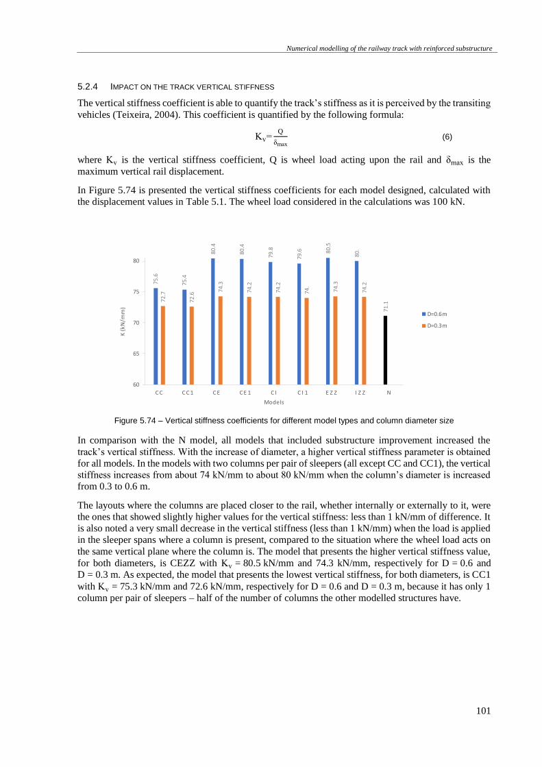
Numerical modelling of the railway track with reinforced substructure
101
5.2.4 IMPACT ON THE TRACK VERTICAL STIFFNESS
The vertical stiffness coefficient is able to quantify the track’s stiffness as it is perceived by the transiting
vehicles (Teixeira, 2004). This coefficient is quantified by the following formula:
Kv=Q
δmax (6)
where Kv is the vertical stiffness coefficient, Q is wheel load acting upon the rail and δmax is the
maximum vertical rail displacement.
In Figure 5.74 is presented the vertical stiffness coefficients for each model designed, calculated with
the displacement values in Table 5.1. The wheel load considered in the calculations was 100 kN.
Figure 5.74 – Vertical stiffness coefficients for different model types and column diameter size
In comparison with the N model, all models that included substructure improvement increased the
track’s vertical stiffness. With the increase of diameter, a higher vertical stiffness parameter is obtained
for all models. In the models with two columns per pair of sleepers (all except CC and CC1), the vertical
stiffness increases from about 74 kN/mm to about 80 kN/mm when the column’s diameter is increased
from 0.3 to 0.6 m.
The layouts where the columns are placed closer to the rail, whether internally or externally to it, were
the ones that showed slightly higher values for the vertical stiffness: less than 1 kN/mm of difference. It
is also noted a very small decrease in the vertical stiffness (less than 1 kN/mm) when the load is applied
in the sleeper spans where a column is present, compared to the situation where the wheel load acts on
the same vertical plane where the column is. The model that presents the higher vertical stiffness value,
for both diameters, is CEZZ with Kv = 80.5 kN/mm and 74.3 kN/mm, respectively for D = 0.6 and
D = 0.3 m. As expected, the model that presents the lowest vertical stiffness, for both diameters, is CC1
with Kv = 75.3 kN/mm and 72.6 kN/mm, respectively for D = 0.6 and D = 0.3 m, because it has only 1
column per pair of sleepers – half of the number of columns the other modelled structures have.
75.6
75.4
80.4
80.4
79.8
79.6 80
.5
80
.
71
.1
72.7
72.6
74.3
74.2
74
.2
74.
74.3
74.2
60
65
70
75
80
C C C C 1 C E C E 1 C I C I 1 E Z Z I Z Z N
K (
kN
/mm
)
Models
D=0.6m
D=0.3m
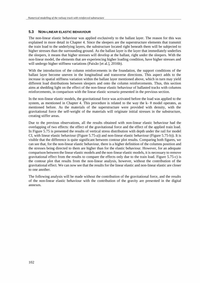
Numerical modelling of the railway track with reinforced substructure
102
5.3 NON-LINEAR ELASTIC BEHAVIOUR
The non-linear elastic behaviour was applied exclusively to the ballast layer. The reason for this was
explained in more detail in Chapter 4. Since the sleepers are the superstructure elements that transmit
the train load to the underlying layers, the substructure located right beneath them will be subjected to
higher stresses than the surrounding ground. As the ballast layer is the layer that immediately underlies
the sleepers, it means that higher stresses will develop at the ballast, right under the sleepers. With the
non-linear model, the elements that are experiencing higher loading condition, have higher stresses and
will undergo higher stiffness variations (Paixão [et al.], 2016b).
With the introduction of the column reinforcements in the foundation, the support conditions of the
ballast layer become uneven in the longitudinal and transverse directions. This aspect adds to the
increase in spatial stiffness variation within the ballast layer mentioned above, which in turn may yield
different load distributions between sleepers and onto the column reinforcements. Thus, this section
aims at shedding light on the effect of the non-linear elastic behaviour of ballasted tracks with columns
reinforcements, in comparison with the linear elastic scenario presented in the previous section.
In the non-linear elastic models, the gravitational force was activated before the load was applied to the
system, as mentioned in Chapter 4. This procedure is related to the way the k- θ model operates, as
mentioned before. As the materials of the superstructure were provided with density, with the
gravitational force the self-weight of the materials will originate initial stresses in the substructure,
creating stiffer areas.
Due to the previous observations, all the results obtained with non-linear elastic behaviour had the
overlapping of two effects: the effect of the gravitational force and the effect of the applied train load.
In Figure 5.75 is presented the results of vertical stress distribution with depth under the rail for model
CI, with linear elastic behaviour (Figure 5.75-a)) and non-linear elastic behaviour (Figure 5.75-b)). It is
visible that the difference is quite significant between contour plot results. Comparing both figures, we
can see that, for the non-linear elastic behaviour, there is a higher definition of the columns position and
the stresses being directed to them are higher than for the elastic behaviour. However, for an adequate
comparison between the linear elastic models and the non-linear elastic models, it is necessary to remove
gravitational effect from the results to compare the effects only due to the train load. Figure 5.75-c) is
the contour plot that results from the non-linear analysis, however, without the contribution of the
gravitational effect. We can now see that the results for the linear elastic and non-linear elastic are closer
to one another.
The following analysis will be made without the contribution of the gravitational force, and the results
of the non-linear elastic behaviour with the contribution of the gravity are presented in the digital
annexes.
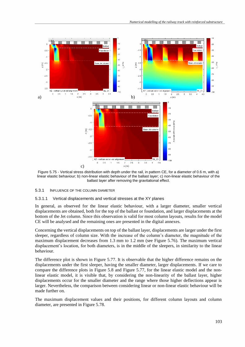
Numerical modelling of the railway track with reinforced substructure
103
a) b)
c)
Figure 5.75 - Vertical stress distribution with depth under the rail, in pattern CE, for a diameter of 0.6 m, with a) linear elastic behaviour; b) non-linear elastic behaviour of the ballast layer; c) non-linear elastic behaviour of the
ballast layer after removing the gravitational effect.
5.3.1 INFLUENCE OF THE COLUMN DIAMETER
5.3.1.1 Vertical displacements and vertical stresses at the XY planes
In general, as observed for the linear elastic behaviour, with a larger diameter, smaller vertical
displacements are obtained, both for the top of the ballast or foundation, and larger displacements at the
bottom of the Jet column. Since this observation is valid for most column layouts, results for the model
CE will be analysed and the remaining ones are presented in the digital annexes.
Concerning the vertical displacements on top of the ballast layer, displacements are larger under the first
sleeper, regardless of column size. With the increase of the column’s diameter, the magnitude of the
maximum displacement decreases from 1.3 mm to 1.2 mm (see Figure 5.76). The maximum vertical
displacement’s location, for both diameters, is in the middle of the sleepers, in similarity to the linear
behaviour.
The difference plot is shown in Figure 5.77. It is observable that the higher difference remains on the
displacements under the first sleeper, having the smaller diameter, larger displacements. If we care to
compare the difference plots in Figure 5.8 and Figure 5.77, for the linear elastic model and the non-
linear elastic model, it is visible that, by considering the non-linearity of the ballast layer, higher
displacements occur for the smaller diameter and the range where those higher deflections appear is
larger. Nevertheless, the comparison between considering linear or non-linear elastic behaviour will be
made further on.
The maximum displacement values and their positions, for different column layouts and column
diameter, are presented in Figure 5.78.
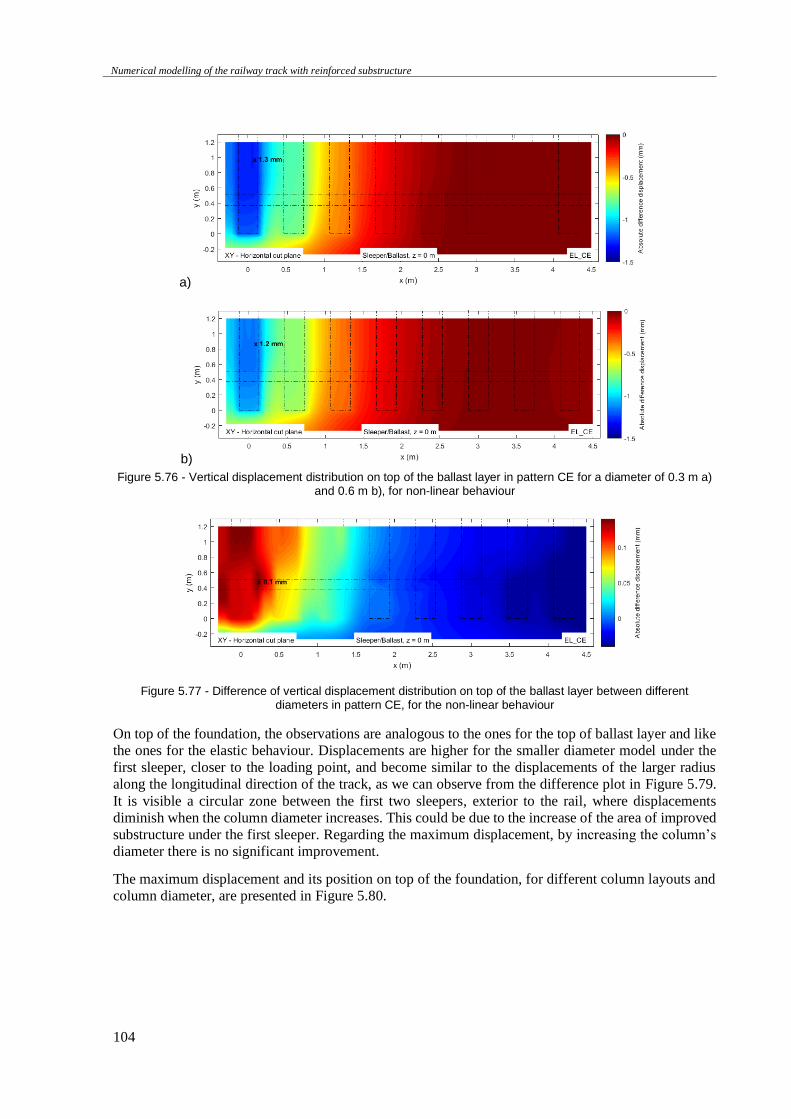
Numerical modelling of the railway track with reinforced substructure
104
a)
b)
Figure 5.76 - Vertical displacement distribution on top of the ballast layer in pattern CE for a diameter of 0.3 m a) and 0.6 m b), for non-linear behaviour
Figure 5.77 - Difference of vertical displacement distribution on top of the ballast layer between different diameters in pattern CE, for the non-linear behaviour
On top of the foundation, the observations are analogous to the ones for the top of ballast layer and like
the ones for the elastic behaviour. Displacements are higher for the smaller diameter model under the
first sleeper, closer to the loading point, and become similar to the displacements of the larger radius
along the longitudinal direction of the track, as we can observe from the difference plot in Figure 5.79.
It is visible a circular zone between the first two sleepers, exterior to the rail, where displacements
diminish when the column diameter increases. This could be due to the increase of the area of improved
substructure under the first sleeper. Regarding the maximum displacement, by increasing the column’s
diameter there is no significant improvement.
The maximum displacement and its position on top of the foundation, for different column layouts and
column diameter, are presented in Figure 5.80.
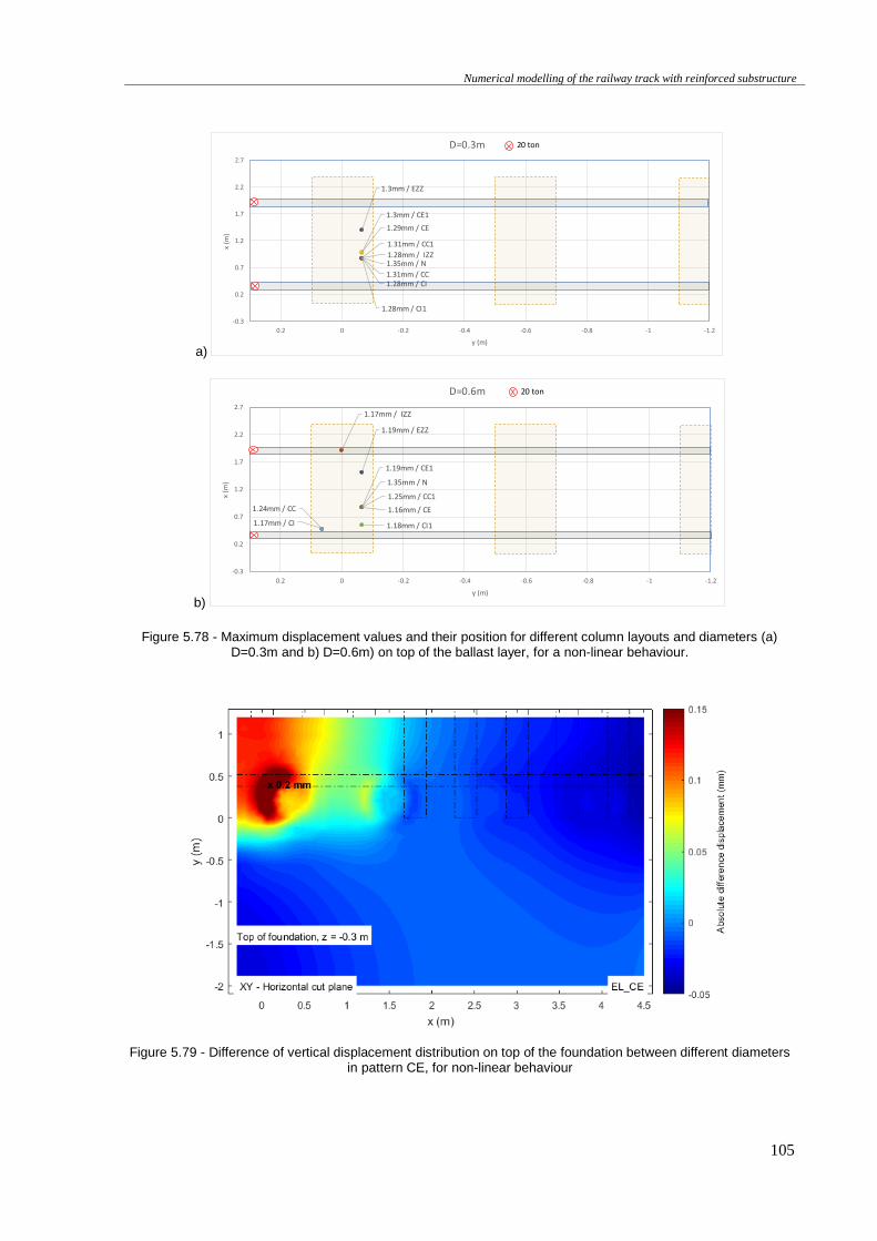
Numerical modelling of the railway track with reinforced substructure
105
a)
b)
Figure 5.78 - Maximum displacement values and their position for different column layouts and diameters (a) D=0.3m and b) D=0.6m) on top of the ballast layer, for a non-linear behaviour.
Figure 5.79 - Difference of vertical displacement distribution on top of the foundation between different diameters in pattern CE, for non-linear behaviour
1.31mm / CC
1.31mm / CC1
1.29mm / CE
1.3mm / CE1
1.28mm / CI
1.28mm / CI1
1.3mm / EZZ
1.28mm / IZZ1.35mm / N
-0.3
0.2
0.7
1.2
1.7
2.2
2.7
-1.2-1-0.8-0.6-0.4-0.200.2
x (m
)
y (m)
D=0.3m 20 ton
1.24mm / CC
1.25mm / CC1
1.16mm / CE
1.19mm / CE1
1.17mm / CI 1.18mm / CI1
1.19mm / EZZ
1.17mm / IZZ
1.35mm / N
-0.3
0.2
0.7
1.2
1.7
2.2
2.7
-1.2-1-0.8-0.6-0.4-0.200.2
x (m
)
y (m)
D=0.6m 20 ton
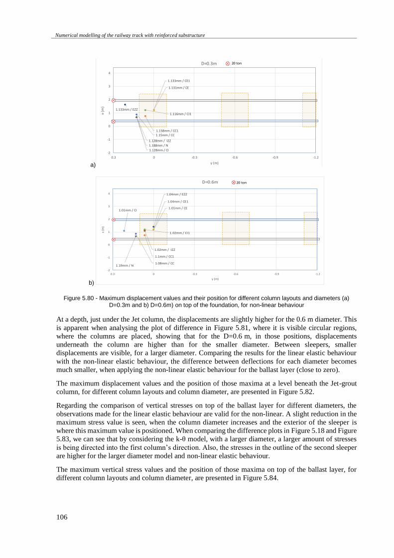
Numerical modelling of the railway track with reinforced substructure
106
a)
b)
Figure 5.80 - Maximum displacement values and their position for different column layouts and diameters (a) D=0.3m and b) D=0.6m) on top of the foundation, for non-linear behaviour
At a depth, just under the Jet column, the displacements are slightly higher for the 0.6 m diameter. This
is apparent when analysing the plot of difference in Figure 5.81, where it is visible circular regions,
where the columns are placed, showing that for the D=0.6 m, in those positions, displacements
underneath the column are higher than for the smaller diameter. Between sleepers, smaller
displacements are visible, for a larger diameter. Comparing the results for the linear elastic behaviour
with the non-linear elastic behaviour, the difference between deflections for each diameter becomes
much smaller, when applying the non-linear elastic behaviour for the ballast layer (close to zero).
The maximum displacement values and the position of those maxima at a level beneath the Jet-grout
column, for different column layouts and column diameter, are presented in Figure 5.82.
Regarding the comparison of vertical stresses on top of the ballast layer for different diameters, the
observations made for the linear elastic behaviour are valid for the non-linear. A slight reduction in the
maximum stress value is seen, when the column diameter increases and the exterior of the sleeper is
where this maximum value is positioned. When comparing the difference plots in Figure 5.18 and Figure
5.83, we can see that by considering the k-θ model, with a larger diameter, a larger amount of stresses
is being directed into the first column’s direction. Also, the stresses in the outline of the second sleeper
are higher for the larger diameter model and non-linear elastic behaviour.
The maximum vertical stress values and the position of those maxima on top of the ballast layer, for
different column layouts and column diameter, are presented in Figure 5.84.
1.15mm / CC1.158mm / CC1
1.131mm / CE
1.133mm / CE1
1.128mm / CI
1.116mm / CI11.133mm / EZZ
1.128mm / IZZ
1.188mm / N
-2
-1
0
1
2
3
4
-1.2-0.9-0.6-0.300.3
x (m
)
y (m)
D=0.3m 20 ton
1.08mm / CC
1.1mm / CC1
1.01mm / CE
1.04mm / CE1
1.01mm / CI
1.02mm / CI1
1.04mm / EZZ
1.02mm / IZZ
1.19mm / N
-2
-1
0
1
2
3
4
-1.2-0.9-0.6-0.300.3
x (m
)
y (m)
D=0.6m 20 ton
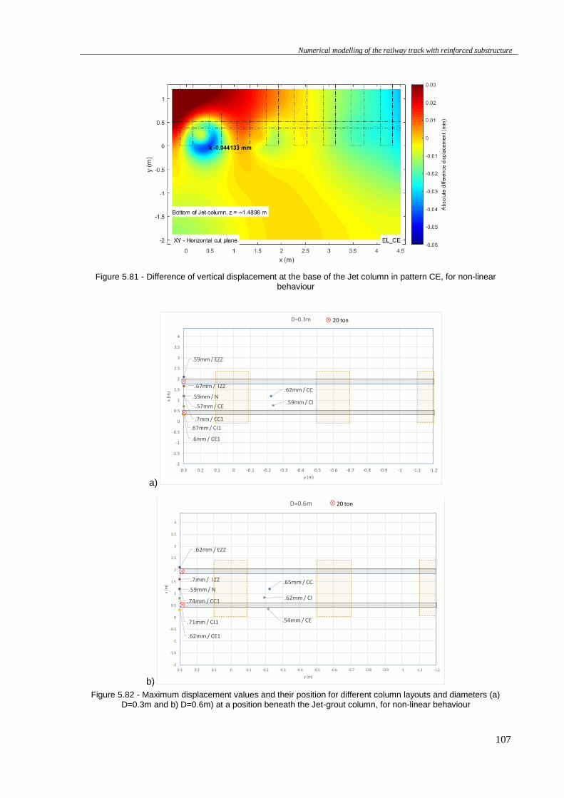
Numerical modelling of the railway track with reinforced substructure
107
Figure 5.81 - Difference of vertical displacement at the base of the Jet column in pattern CE, for non-linear behaviour
a)
b)
Figure 5.82 - Maximum displacement values and their position for different column layouts and diameters (a) D=0.3m and b) D=0.6m) at a position beneath the Jet-grout column, for non-linear behaviour
.62mm / CC
.7mm / CC1
.57mm / CE
.6mm / CE1
.59mm / CI
.67mm / CI1
.59mm / EZZ
.67mm / IZZ
.59mm / N
-2
-1.5
-1
-0.5
0
0.5
1
1.5
2
2.5
3
3.5
4
-1.2-1.1-1-0.9-0.8-0.7-0.6-0.5-0.4-0.3-0.2-0.100.10.20.3
x (m
)
y (m)
D=0.3m 20 ton
.65mm / CC
.74mm / CC1
.54mm / CE
.62mm / CE1
.62mm / CI
.71mm / CI1
.62mm / EZZ
.7mm / IZZ
.59mm / N
-2
-1.5
-1
-0.5
0
0.5
1
1.5
2
2.5
3
3.5
4
-1.2-1.1-1-0.9-0.8-0.7-0.6-0.5-0.4-0.3-0.2-0.100.10.20.3
x (m
)
y (m)
D=0.6m 20 ton
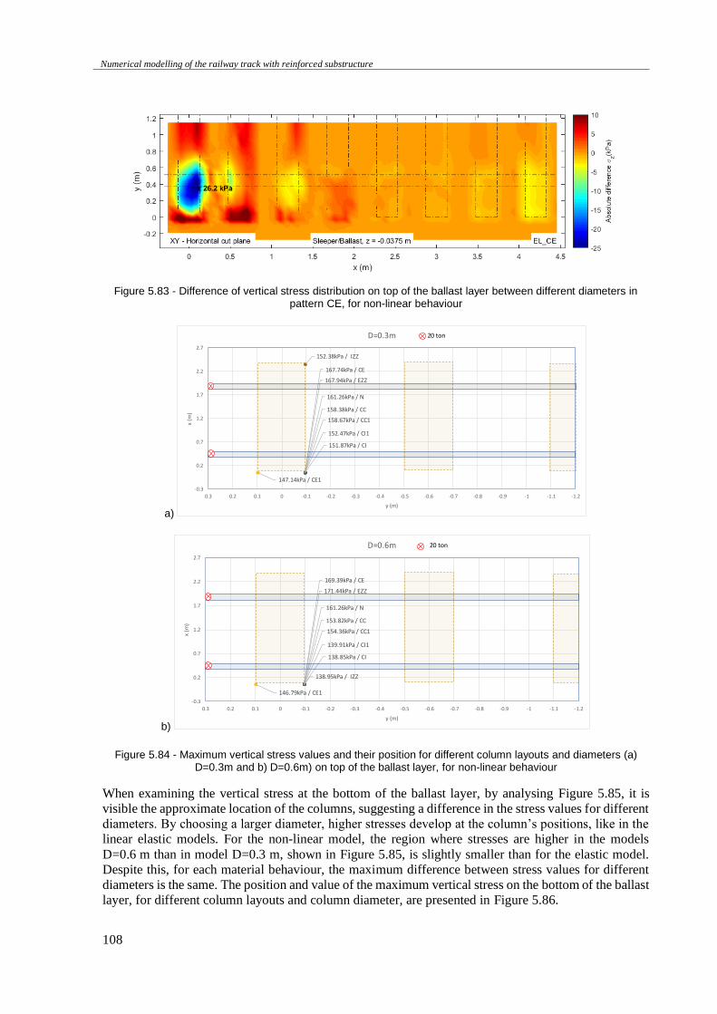
Numerical modelling of the railway track with reinforced substructure
108
Figure 5.83 - Difference of vertical stress distribution on top of the ballast layer between different diameters in pattern CE, for non-linear behaviour
a)
b)
Figure 5.84 - Maximum vertical stress values and their position for different column layouts and diameters (a) D=0.3m and b) D=0.6m) on top of the ballast layer, for non-linear behaviour
When examining the vertical stress at the bottom of the ballast layer, by analysing Figure 5.85, it is
visible the approximate location of the columns, suggesting a difference in the stress values for different
diameters. By choosing a larger diameter, higher stresses develop at the column’s positions, like in the
linear elastic models. For the non-linear model, the region where stresses are higher in the models
D=0.6 m than in model D=0.3 m, shown in Figure 5.85, is slightly smaller than for the elastic model.
Despite this, for each material behaviour, the maximum difference between stress values for different
diameters is the same. The position and value of the maximum vertical stress on the bottom of the ballast
layer, for different column layouts and column diameter, are presented in Figure 5.86.
158.38kPa / CC
158.67kPa / CC1
167.74kPa / CE
147.14kPa / CE1
151.87kPa / CI
152.47kPa / CI1
167.94kPa / EZZ
152.38kPa / IZZ
161.26kPa / N
-0.3
0.2
0.7
1.2
1.7
2.2
2.7
-1.2-1.1-1-0.9-0.8-0.7-0.6-0.5-0.4-0.3-0.2-0.100.10.20.3
x (m
)
y (m)
D=0.3m 20 ton
153.82kPa / CC
154.36kPa / CC1
169.39kPa / CE
146.79kPa / CE1
138.85kPa / CI
139.91kPa / CI1
171.44kPa / EZZ
138.95kPa / IZZ
161.26kPa / N
-0.3
0.2
0.7
1.2
1.7
2.2
2.7
-1.2-1.1-1-0.9-0.8-0.7-0.6-0.5-0.4-0.3-0.2-0.100.10.20.3
x (m
)
y (m)
D=0.6m 20 ton

Numerical modelling of the railway track with reinforced substructure
109
Figure 5.85 - Difference of vertical stress distribution at the bottom of the ballast layer for different diameters in pattern CE, for non-linear behaviour
a)
b)
Figure 5.86 - Maximum vertical stress values and their position for different column layouts and diameters (a) D=0.3m and b) D=0.6m) on bottom of the ballast layer, for non-linear behaviour
80.08kPa / CC
60.07kPa / CC1
99.32kPa / CE
78.82kPa / CE1
85.74kPa / CI
64.21kPa / CI1
98.99kPa / EZZ
86.22kPa / IZZ
55.05kPa / N
-0.5
0
0.5
1
1.5
2
2.5
3
-1.2-0.9-0.6-0.300.3
x (m
)
y (m)
D=0.3m 20 ton
94.09kPa / CC
73.88kPa / CC1
107.63kPa / CE
90.84kPa / CE1
91.9kPa / CI73.27kPa / CI1
108.87kPa / EZZ
92.63kPa / IZZ
55.05kPa / N
-0.5
0
0.5
1
1.5
2
2.5
3
-1.2-0.9-0.6-0.300.3
x (m
)
y (m)
D=0.6m 20 ton
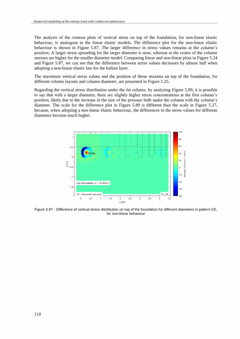
Numerical modelling of the railway track with reinforced substructure
110
The analysis of the contour plots of vertical stress on top of the foundation, for non-linear elastic
behaviour, is analogous to the linear elastic models. The difference plot for the non-linear elastic
behaviour is shown in Figure 5.87. The larger difference in stress values remains at the column’s
position. A larger stress spreading for the larger diameter is seen, whereas at the centre of the column
stresses are higher for the smaller diameter model. Comparing linear and non-linear plots in Figure 5.24
and Figure 5.87, we can see that the difference between stress values decreases by almost half when
adopting a non-linear elastic law for the ballast layer.
The maximum vertical stress values and the position of those maxima on top of the foundation, for
different column layouts and column diameter, are presented in Figure 5.25.
Regarding the vertical stress distribution under the Jet column, by analysing Figure 5.89, it is possible
to say that with a larger diameter, there are slightly higher stress concentrations at the first column’s
position, likely due to the increase in the size of the pressure bulb under the column with the column’s
diameter. The scale for the difference plot in Figure 5.89 is different than the scale in Figure 5.27,
because, when adopting a non-linear elastic behaviour, the differences in the stress values for different
diameters become much higher.
Figure 5.87 - Difference of vertical stress distribution on top of the foundation for different diameters in pattern CE, for non-linear behaviour
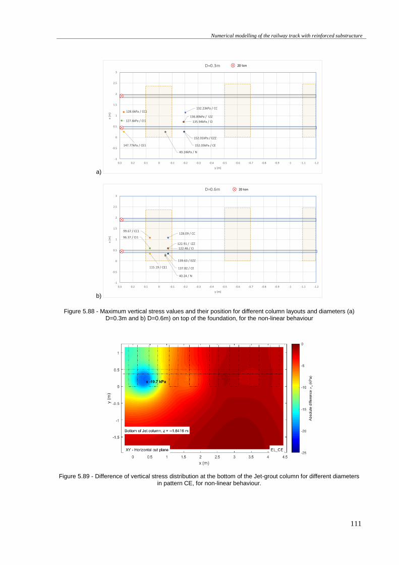
Numerical modelling of the railway track with reinforced substructure
111
a)
b)
Figure 5.88 - Maximum vertical stress values and their position for different column layouts and diameters (a) D=0.3m and b) D=0.6m) on top of the foundation, for the non-linear behaviour
Figure 5.89 - Difference of vertical stress distribution at the bottom of the Jet-grout column for different diameters in pattern CE, for non-linear behaviour.
132.23kPa / CC128.6kPa / CC1
152.03kPa / CE147.77kPa / CE1
135.94kPa / CI127.6kPa / CI1
152.01kPa / EZZ
136.89kPa / IZZ
40.24kPa / N
-1
-0.5
0
0.5
1
1.5
2
2.5
3
-1.2-1.1-1-0.9-0.8-0.7-0.6-0.5-0.4-0.3-0.2-0.100.10.20.3
x (m
)
y (m)
D=0.3m 20 ton
128.09 / CC99.67 / CC1
137.82 / CE115.19 / CE1
122.46 / CI
96.37 / CI1
139.63 / EZZ
122.91 / IZZ
40.24 / N
-1
-0.5
0
0.5
1
1.5
2
2.5
3
-1.2-1.1-1-0.9-0.8-0.7-0.6-0.5-0.4-0.3-0.2-0.100.10.20.3
x (m
)
y (m)
D=0.6m 20 ton
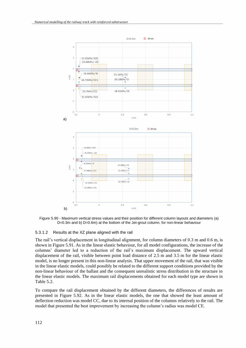
Numerical modelling of the railway track with reinforced substructure
112
a)
b)
Figure 5.90 - Maximum vertical stress values and their position for different column layouts and diameters (a) D=0.3m and b) D=0.6m) at the bottom of the Jet-grout column, for non-linear behaviour
5.3.1.2 Results at the XZ plane aligned with the rail
The rail’s vertical displacement in longitudinal alignment, for column diameters of 0.3 m and 0.6 m, is
shown in Figure 5.91. As in the linear elastic behaviour, for all model configurations, the increase of the
columns’ diameter led to a reduction of the rail’s maximum displacement. The upward vertical
displacement of the rail, visible between point load distance of 2.5 m and 3.5 m for the linear elastic
model, is no longer present in this non-linear analysis. That upper movement of the rail, that was visible
in the linear elastic models, could possibly be related to the different support conditions provided by the
non-linear behaviour of the ballast and the consequent unrealistic stress distribution in the structure in
the linear elastic models. The maximum rail displacements obtained for each model type are shown in
Table 5.2.
To compare the rail displacement obtained by the different diameters, the differences of results are
presented in Figure 5.92. As in the linear elastic models, the one that showed the least amount of
deflection reduction was model CC, due to its internal position of the columns relatively to the rail. The
model that presented the best improvement by increasing the column’s radius was model CE.
21.1kPa / CC
24.72kPa / CC1
18.41kPa / CE
21.65kPa / CE1
20.18kPa / CI
23.7kPa / CI1
21.65kPa / EZZ
23.68kPa / IZZ
16.66kPa / N
-2
-1
0
1
2
3
4
-1.2-0.9-0.6-0.300.3
x (m
)
y (m)
D=0.3m 20 ton
23.28kPa / CC
27.48kPa / CC1
19.73kPa / CE
23.59kPa / CE1
21.51kPa / CI
25.52kPa / CI1
23.6kPa / EZZ
25.35kPa / IZZ
16.65kPa / N
-2
-1
0
1
2
3
4
-1.2-0.9-0.6-0.300.3
x (m
)
y (m)
D=0.6m 20 ton
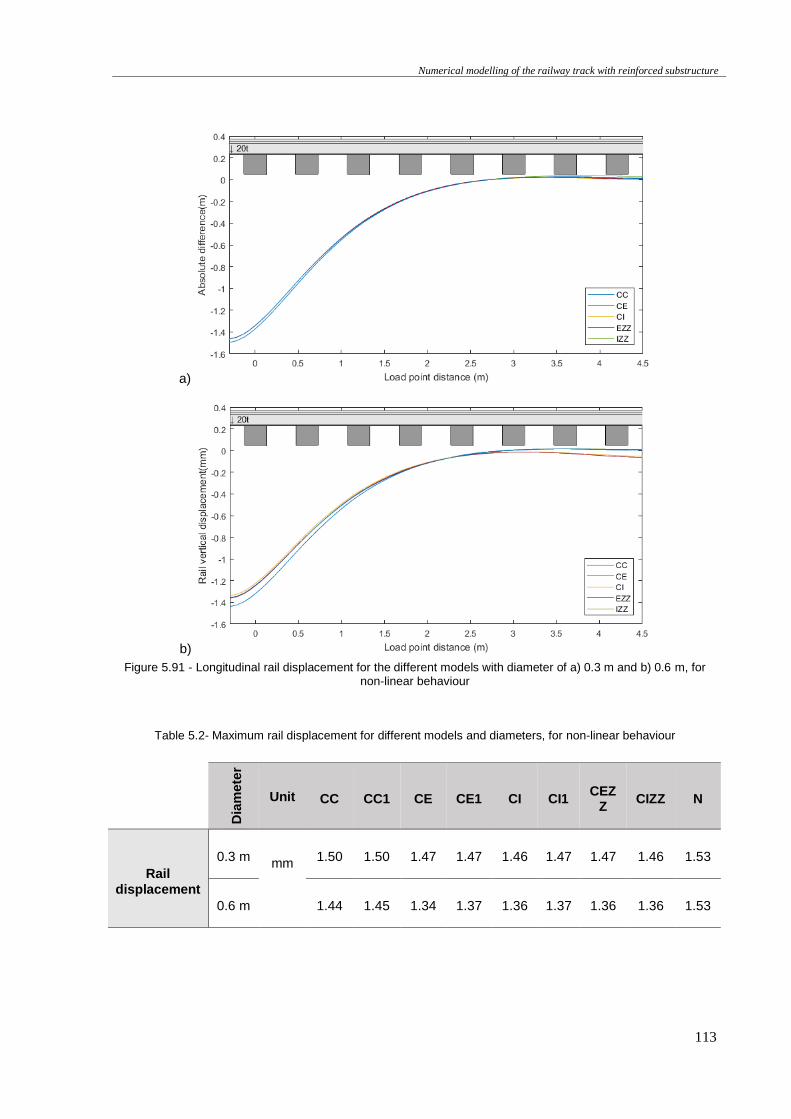
Numerical modelling of the railway track with reinforced substructure
113
a)
b)
Figure 5.91 - Longitudinal rail displacement for the different models with diameter of a) 0.3 m and b) 0.6 m, for non-linear behaviour
Table 5.2- Maximum rail displacement for different models and diameters, for non-linear behaviour
Dia
me
ter
Unit CC CC1 CE CE1 CI CI1 CEZ
Z CIZZ N
Rail
displacement
0.3 m
mm 1.50 1.50 1.47 1.47 1.46 1.47 1.47 1.46 1.53
0.6 m 1.44 1.45 1.34 1.37 1.36 1.37 1.36 1.36 1.53
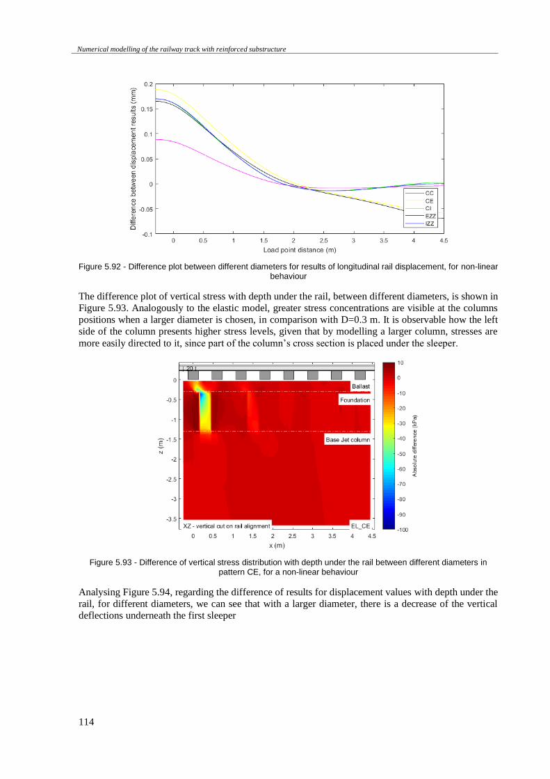
Numerical modelling of the railway track with reinforced substructure
114
Figure 5.92 - Difference plot between different diameters for results of longitudinal rail displacement, for non-linear behaviour
The difference plot of vertical stress with depth under the rail, between different diameters, is shown in
Figure 5.93. Analogously to the elastic model, greater stress concentrations are visible at the columns
positions when a larger diameter is chosen, in comparison with D=0.3 m. It is observable how the left
side of the column presents higher stress levels, given that by modelling a larger column, stresses are
more easily directed to it, since part of the column’s cross section is placed under the sleeper.
Figure 5.93 - Difference of vertical stress distribution with depth under the rail between different diameters in pattern CE, for a non-linear behaviour
Analysing Figure 5.94, regarding the difference of results for displacement values with depth under the
rail, for different diameters, we can see that with a larger diameter, there is a decrease of the vertical
deflections underneath the first sleeper
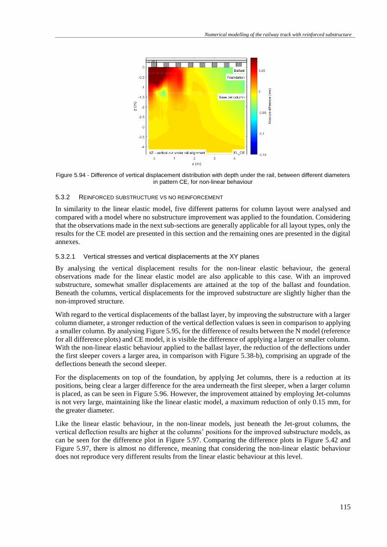
Numerical modelling of the railway track with reinforced substructure
115
Figure 5.94 - Difference of vertical displacement distribution with depth under the rail, between different diameters in pattern CE, for non-linear behaviour
5.3.2 REINFORCED SUBSTRUCTURE VS NO REINFORCEMENT
In similarity to the linear elastic model, five different patterns for column layout were analysed and
compared with a model where no substructure improvement was applied to the foundation. Considering
that the observations made in the next sub-sections are generally applicable for all layout types, only the
results for the CE model are presented in this section and the remaining ones are presented in the digital
annexes.
5.3.2.1 Vertical stresses and vertical displacements at the XY planes
By analysing the vertical displacement results for the non-linear elastic behaviour, the general
observations made for the linear elastic model are also applicable to this case. With an improved
substructure, somewhat smaller displacements are attained at the top of the ballast and foundation.
Beneath the columns, vertical displacements for the improved substructure are slightly higher than the
non-improved structure.
With regard to the vertical displacements of the ballast layer, by improving the substructure with a larger
column diameter, a stronger reduction of the vertical deflection values is seen in comparison to applying
a smaller column. By analysing Figure 5.95, for the difference of results between the N model (reference
for all difference plots) and CE model, it is visible the difference of applying a larger or smaller column.
With the non-linear elastic behaviour applied to the ballast layer, the reduction of the deflections under
the first sleeper covers a larger area, in comparison with Figure 5.38-b), comprising an upgrade of the
deflections beneath the second sleeper.
For the displacements on top of the foundation, by applying Jet columns, there is a reduction at its
positions, being clear a larger difference for the area underneath the first sleeper, when a larger column
is placed, as can be seen in Figure 5.96. However, the improvement attained by employing Jet-columns
is not very large, maintaining like the linear elastic model, a maximum reduction of only 0.15 mm, for
the greater diameter.
Like the linear elastic behaviour, in the non-linear models, just beneath the Jet-grout columns, the
vertical deflection results are higher at the columns’ positions for the improved substructure models, as
can be seen for the difference plot in Figure 5.97. Comparing the difference plots in Figure 5.42 and
Figure 5.97, there is almost no difference, meaning that considering the non-linear elastic behaviour
does not reproduce very different results from the linear elastic behaviour at this level.
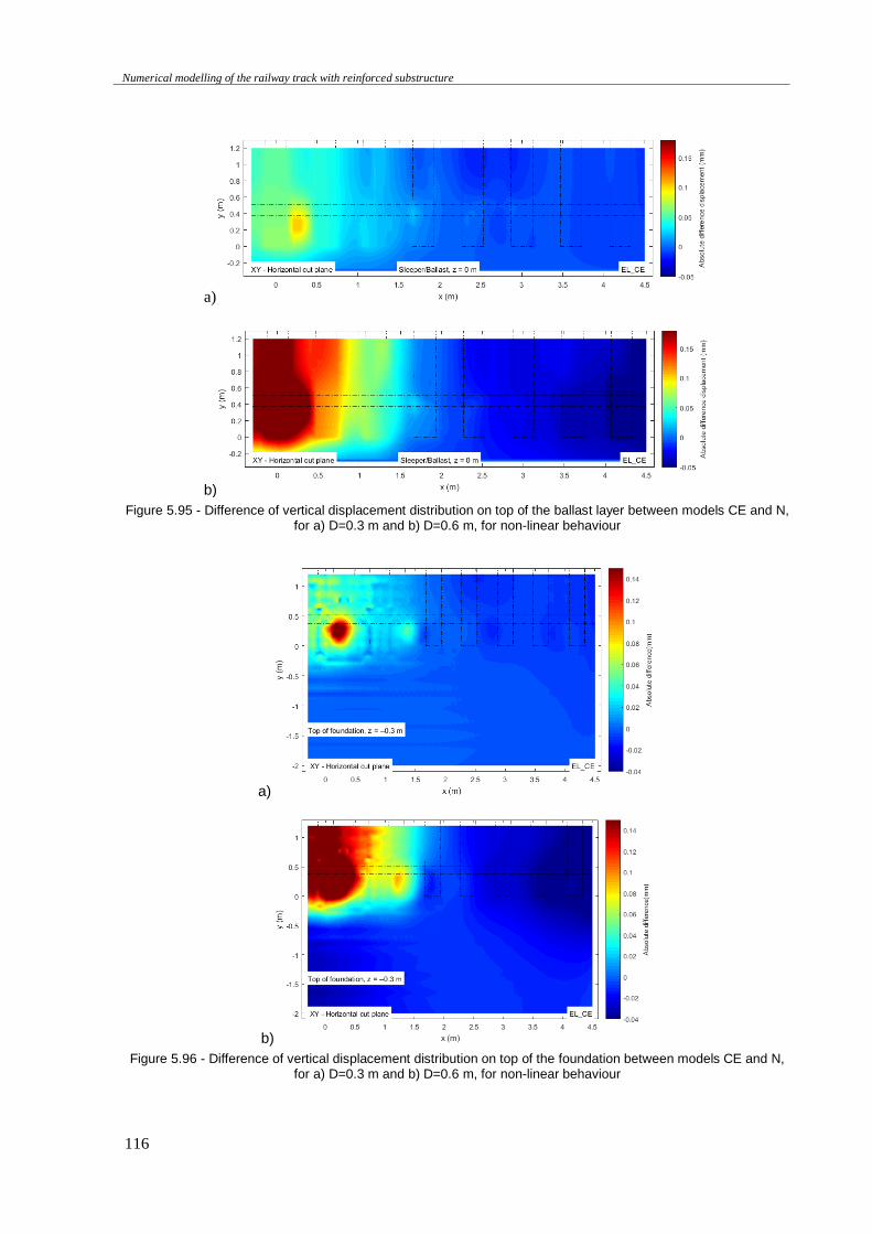
Numerical modelling of the railway track with reinforced substructure
116
a)
b)
Figure 5.95 - Difference of vertical displacement distribution on top of the ballast layer between models CE and N, for a) D=0.3 m and b) D=0.6 m, for non-linear behaviour
a)
b)
Figure 5.96 - Difference of vertical displacement distribution on top of the foundation between models CE and N, for a) D=0.3 m and b) D=0.6 m, for non-linear behaviour
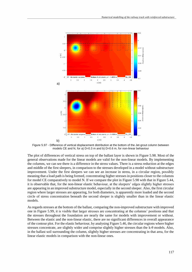
Numerical modelling of the railway track with reinforced substructure
117
a)
b)
Figure 5.97 - Difference of vertical displacement distribution at the bottom of the Jet-grout column between models CE and N, for a) D=0.3 m and b) D=0.6 m, for non-linear behaviour
The plot of differences of vertical stress on top of the ballast layer is shown in Figure 5.98. Most of the
general observations made for the linear models are valid for the non-linear models. By implementing
the columns, we can see there is a difference in the stress values. There is a stress reduction at the edges
and middle of the first sleepers, in comparison to the stresses developed in a model without substructure
improvement. Under the first sleepers we can see an increase in stress, in a circular region, possibly
meaning that a load path is being formed, concentrating higher stresses in positions closer to the columns
for model CE comparatively to model N. If we compare the plot in Figure 5.98 with that in Figure 5.44,
it is observable that, for the non-linear elastic behaviour, at the sleepers’ edges slightly higher stresses
are appearing in an improved substructure model, especially in the second sleeper. Also, the first circular
region where larger stresses are appearing, for both diameters, is apparently more loaded and the second
circle of stress concentration beneath the second sleeper is slightly smaller than in the linear elastic
models.
As regards stresses at the bottom of the ballast, comparing the non-improved substructure with improved
one in Figure 5.99, it is visible that larger stresses are concentrating at the columns’ positions and that
the stresses throughout the foundation are nearly the same for models with improvement or without.
Between the elastic and the non-linear elastic, there are no significant differences in overall appearance
of the contour plot. For the elastic behaviour, by analysing Figure 5.46, the circular regions where higher
stresses concentrate, are slightly wider and comprise slightly higher stresses than the k-θ models. Also,
in the ballast soil surrounding the column, slightly higher stresses are concentrating in that area, for the
linear elastic models in comparison with the non-linear ones.
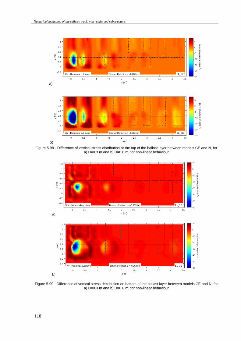
Numerical modelling of the railway track with reinforced substructure
118
a)
b)
Figure 5.98 - Difference of vertical stress distribution at the top of the ballast layer between models CE and N, for a) D=0.3 m and b) D=0.6 m, for non-linear behaviour
a)
b)
Figure 5.99 - Difference of vertical stress distribution on bottom of the ballast layer between models CE and N, for a) D=0.3 m and b) D=0.6 m, for non-linear behaviour
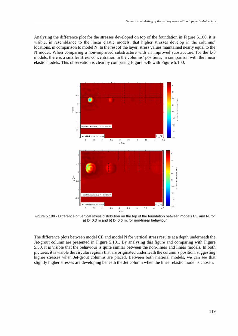
Numerical modelling of the railway track with reinforced substructure
119
Analysing the difference plot for the stresses developed on top of the foundation in Figure 5.100, it is
visible, in resemblance to the linear elastic models, that higher stresses develop in the columns’
locations, in comparison to model N. In the rest of the layer, stress values maintained nearly equal to the
N model. When comparing a non-improved substructure with an improved substructure, for the k-θ
models, there is a smaller stress concentration in the columns’ positions, in comparison with the linear
elastic models. This observation is clear by comparing Figure 5.48 with Figure 5.100.
Figure 5.100 - Difference of vertical stress distribution on the top of the foundation between models CE and N, for
a) D=0.3 m and b) D=0.6 m, for non-linear behaviour
The difference plots between model CE and model N for vertical stress results at a depth underneath the
Jet-grout column are presented in Figure 5.101. By analysing this figure and comparing with Figure
5.50, it is visible that the behaviour is quite similar between the non-linear and linear models. In both
pictures, it is visible the circular regions that are originated underneath the column’s position, suggesting
higher stresses when Jet-grout columns are placed. Between both material models, we can see that
slightly higher stresses are developing beneath the Jet column when the linear elastic model is chosen.

Numerical modelling of the railway track with reinforced substructure
120
Figure 5.101 - Difference of vertical stress distribution on the top of the foundation between models CE and N, for a) D=0.3 m and b) D=0.6 m, for non-linear behaviour
5.3.2.2 Vertical stresses and vertical displacements at the XZ plane aligned with the rail
Regarding the rail’s vertical displacement in the longitudinal alignment, whether we consider a non-
linear or linear law for the ballast’s behaviour, by implementing the Jet-grout columns, smaller rail
displacements were obtained for all models. In the non-linear models, there is a slight difference,
performance-wise, if we chose different column diameters. When opting for a smaller column, the
interior placed layouts (CI and CIZZ) showed a higher reduction in rail displacement, compared with
no improvement at all. By increasing the column’s diameter, the one that showed better performance
was the model CE, reducing rail displacement in almost 0.2 mm, as we can see in Figure 5.102.
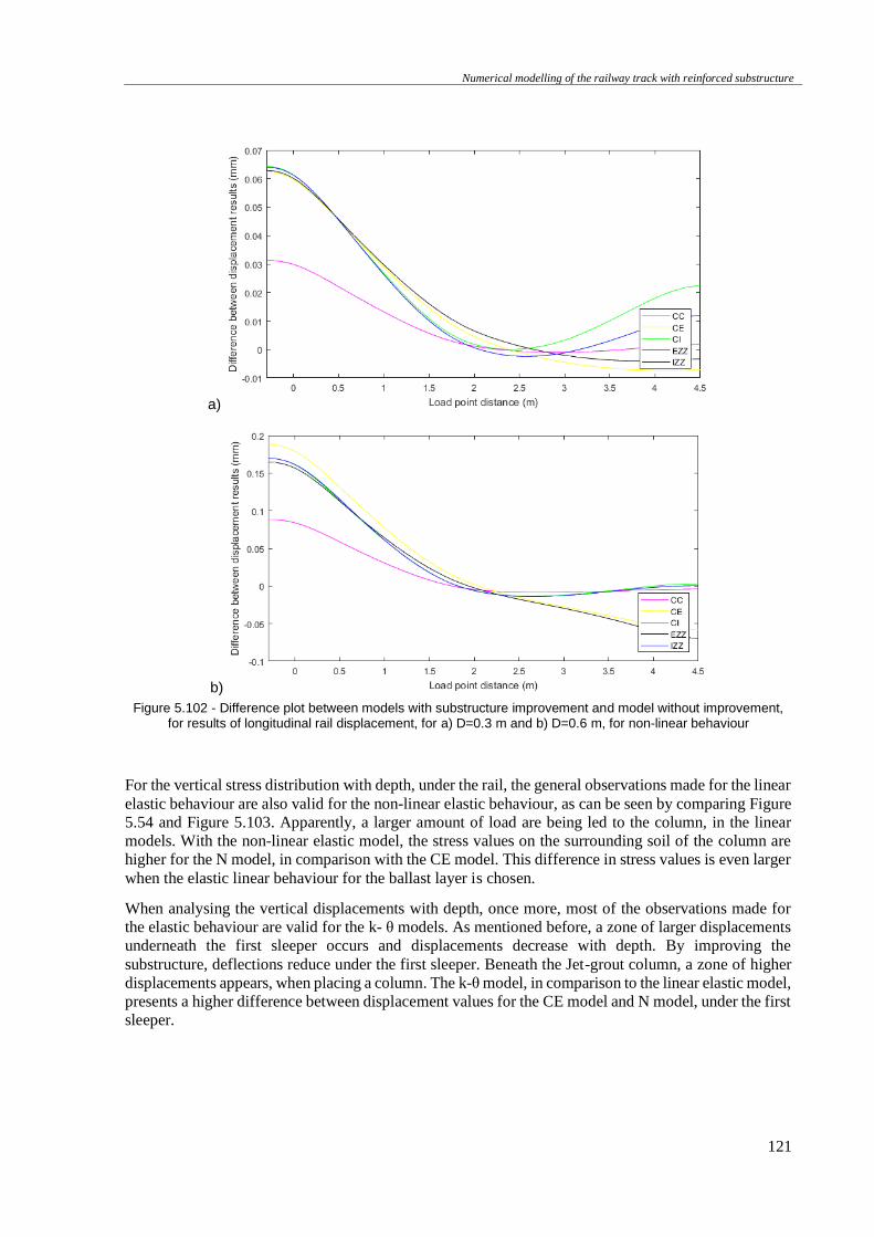
Numerical modelling of the railway track with reinforced substructure
121
a)
b)
Figure 5.102 - Difference plot between models with substructure improvement and model without improvement, for results of longitudinal rail displacement, for a) D=0.3 m and b) D=0.6 m, for non-linear behaviour
For the vertical stress distribution with depth, under the rail, the general observations made for the linear
elastic behaviour are also valid for the non-linear elastic behaviour, as can be seen by comparing Figure
5.54 and Figure 5.103. Apparently, a larger amount of load are being led to the column, in the linear
models. With the non-linear elastic model, the stress values on the surrounding soil of the column are
higher for the N model, in comparison with the CE model. This difference in stress values is even larger
when the elastic linear behaviour for the ballast layer is chosen.
When analysing the vertical displacements with depth, once more, most of the observations made for
the elastic behaviour are valid for the k- θ models. As mentioned before, a zone of larger displacements
underneath the first sleeper occurs and displacements decrease with depth. By improving the
substructure, deflections reduce under the first sleeper. Beneath the Jet-grout column, a zone of higher
displacements appears, when placing a column. The k-θ model, in comparison to the linear elastic model,
presents a higher difference between displacement values for the CE model and N model, under the first
sleeper.
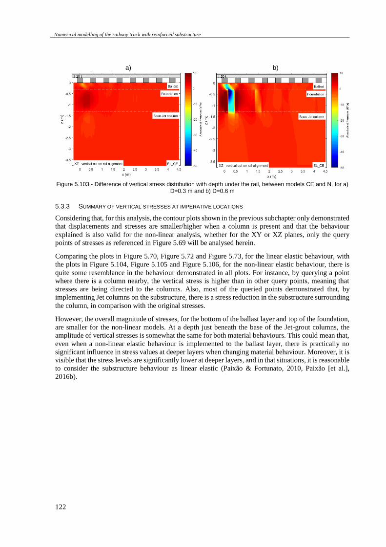
Numerical modelling of the railway track with reinforced substructure
122
a)
b)
Figure 5.103 - Difference of vertical stress distribution with depth under the rail, between models CE and N, for a)
D=0.3 m and b) D=0.6 m
5.3.3 SUMMARY OF VERTICAL STRESSES AT IMPERATIVE LOCATIONS
Considering that, for this analysis, the contour plots shown in the previous subchapter only demonstrated
that displacements and stresses are smaller/higher when a column is present and that the behaviour
explained is also valid for the non-linear analysis, whether for the XY or XZ planes, only the query
points of stresses as referenced in Figure 5.69 will be analysed herein.
Comparing the plots in Figure 5.70, Figure 5.72 and Figure 5.73, for the linear elastic behaviour, with
the plots in Figure 5.104, Figure 5.105 and Figure 5.106, for the non-linear elastic behaviour, there is
quite some resemblance in the behaviour demonstrated in all plots. For instance, by querying a point
where there is a column nearby, the vertical stress is higher than in other query points, meaning that
stresses are being directed to the columns. Also, most of the queried points demonstrated that, by
implementing Jet columns on the substructure, there is a stress reduction in the substructure surrounding
the column, in comparison with the original stresses.
However, the overall magnitude of stresses, for the bottom of the ballast layer and top of the foundation,
are smaller for the non-linear models. At a depth just beneath the base of the Jet-grout columns, the
amplitude of vertical stresses is somewhat the same for both material behaviours. This could mean that,
even when a non-linear elastic behaviour is implemented to the ballast layer, there is practically no
significant influence in stress values at deeper layers when changing material behaviour. Moreover, it is
visible that the stress levels are significantly lower at deeper layers, and in that situations, it is reasonable
to consider the substructure behaviour as linear elastic (Paixão & Fortunato, 2010, Paixão [et al.],
2016b).
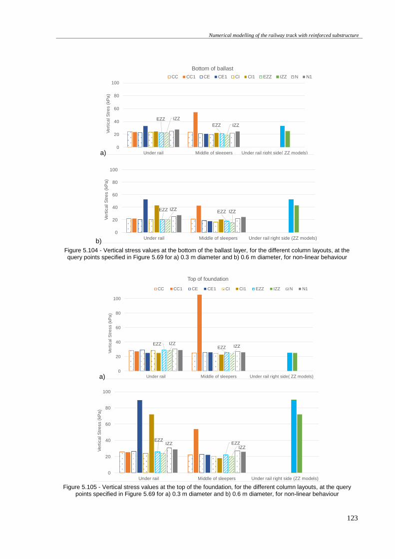
Numerical modelling of the railway track with reinforced substructure
123
a)
b)
Figure 5.104 - Vertical stress values at the bottom of the ballast layer, for the different column layouts, at the query points specified in Figure 5.69 for a) 0.3 m diameter and b) 0.6 m diameter, for non-linear behaviour
a)
Figure 5.105 - Vertical stress values at the top of the foundation, for the different column layouts, at the query
points specified in Figure 5.69 for a) 0.3 m diameter and b) 0.6 m diameter, for non-linear behaviour
EZZ
EZZ
IZZ
IZZ
0
20
40
60
80
100
Under rail Middle of sleepers Under rail right side( ZZ models)
Ve
rtic
al S
tre
s (
kP
a)
Bottom of ballast
CC CC1 CE CE1 CI CI1 EZZ IZZ N N1
EZZ EZZIZZ IZZ
0
20
40
60
80
100
Under rail Middle of sleepers Under rail right side (ZZ models)
Ve
rtic
al S
tre
s (
kP
a)
Bottom of ballast
CC CC1 CE CE1 CI CI1 EZZ IZZ N N1
EZZEZZ
IZZIZZ
0
20
40
60
80
100
Under rail Middle of sleepers Under rail right side( ZZ models)
Ve
rtic
al S
tre
ss (
kP
a)
Top of foundation
CC CC1 CE CE1 CI CI1 EZZ IZZ N N1
EZZEZZIZZ
IZZ
0
20
40
60
80
100
Under rail Middle of sleepers Under rail right side (ZZ models)
Ve
rtic
al S
tre
ss (
kP
a)
Top of foundationCC CC1 CE CE1 CI CI1 EZZ IZZ N N1
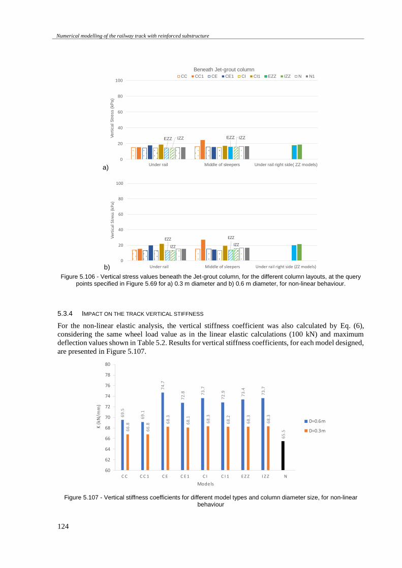
Numerical modelling of the railway track with reinforced substructure
124
a)
b)
Figure 5.106 - Vertical stress values beneath the Jet-grout column, for the different column layouts, at the query points specified in Figure 5.69 for a) 0.3 m diameter and b) 0.6 m diameter, for non-linear behaviour.
5.3.4 IMPACT ON THE TRACK VERTICAL STIFFNESS
For the non-linear elastic analysis, the vertical stiffness coefficient was also calculated by Eq. (6),
considering the same wheel load value as in the linear elastic calculations (100 kN) and maximum
deflection values shown in Table 5.2. Results for vertical stiffness coefficients, for each model designed,
are presented in Figure 5.107.
Figure 5.107 - Vertical stiffness coefficients for different model types and column diameter size, for non-linear behaviour
EZZ EZZIZZ IZZ
0
20
40
60
80
100
Under rail Middle of sleepers Under rail right side( ZZ models)
Ve
rtic
al S
tre
ss (
kP
a)
Beneath Jet-grout column
CC CC1 CE CE1 CI CI1 EZZ IZZ N N1
EZZ EZZ
IZZ IZZ
0
20
40
60
80
100
Under rail Middle of sleepers Under rail right side (ZZ models)
Ver
tica
l St
ress
(kP
a)
Beneath Jet-grout column
CC CC1 CE CE1 CI CI1 EZZ IZZ N N1
69
.5
69
.1
74
.7
72
.8 73
.7
72
.9 73
.4
73
.7
65
.566
.8
66
.8
68
.3
68
.1
68
.3
68
.2
68
.3
68
.3
60
62
64
66
68
70
72
74
76
78
80
C C C C 1 C E C E 1 C I C I 1 E Z Z I Z Z N
K (k
N/m
m)
Models
D=0.6m
D=0.3m
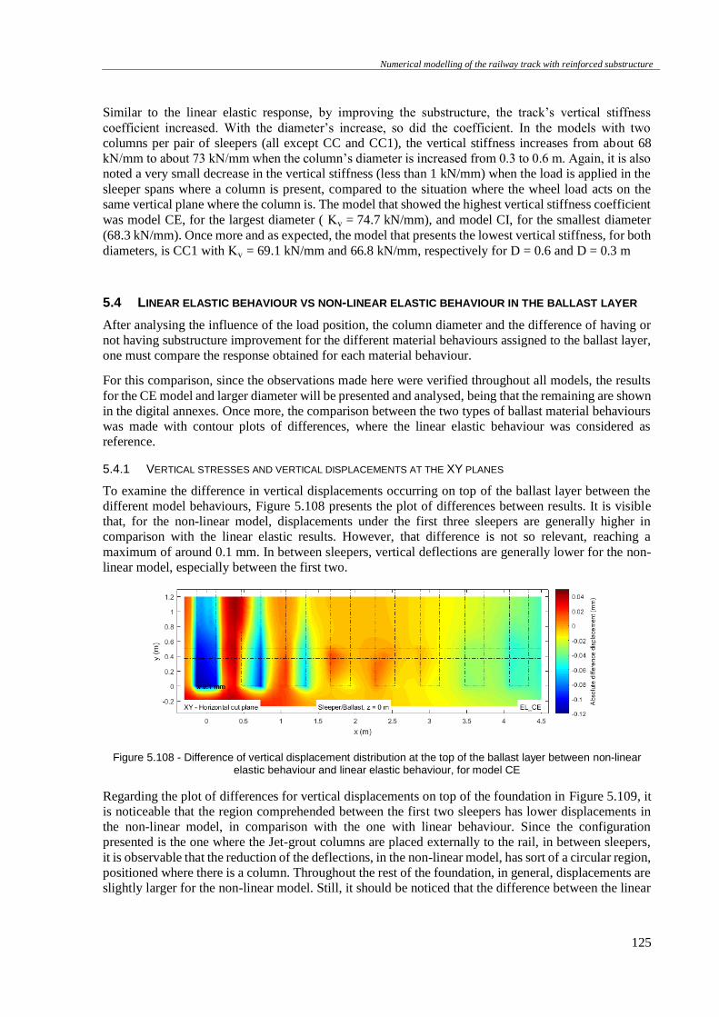
Numerical modelling of the railway track with reinforced substructure
125
Similar to the linear elastic response, by improving the substructure, the track’s vertical stiffness
coefficient increased. With the diameter’s increase, so did the coefficient. In the models with two
columns per pair of sleepers (all except CC and CC1), the vertical stiffness increases from about 68
kN/mm to about 73 kN/mm when the column’s diameter is increased from 0.3 to 0.6 m. Again, it is also
noted a very small decrease in the vertical stiffness (less than 1 kN/mm) when the load is applied in the
sleeper spans where a column is present, compared to the situation where the wheel load acts on the
same vertical plane where the column is. The model that showed the highest vertical stiffness coefficient
was model CE, for the largest diameter ( Kv = 74.7 kN/mm), and model CI, for the smallest diameter
(68.3 kN/mm). Once more and as expected, the model that presents the lowest vertical stiffness, for both
diameters, is CC1 with Kv = 69.1 kN/mm and 66.8 kN/mm, respectively for D = 0.6 and D = 0.3 m
5.4 LINEAR ELASTIC BEHAVIOUR VS NON-LINEAR ELASTIC BEHAVIOUR IN THE BALLAST LAYER
After analysing the influence of the load position, the column diameter and the difference of having or
not having substructure improvement for the different material behaviours assigned to the ballast layer,
one must compare the response obtained for each material behaviour.
For this comparison, since the observations made here were verified throughout all models, the results
for the CE model and larger diameter will be presented and analysed, being that the remaining are shown
in the digital annexes. Once more, the comparison between the two types of ballast material behaviours
was made with contour plots of differences, where the linear elastic behaviour was considered as
reference.
5.4.1 VERTICAL STRESSES AND VERTICAL DISPLACEMENTS AT THE XY PLANES
To examine the difference in vertical displacements occurring on top of the ballast layer between the
different model behaviours, Figure 5.108 presents the plot of differences between results. It is visible
that, for the non-linear model, displacements under the first three sleepers are generally higher in
comparison with the linear elastic results. However, that difference is not so relevant, reaching a
maximum of around 0.1 mm. In between sleepers, vertical deflections are generally lower for the non-
linear model, especially between the first two.
Figure 5.108 - Difference of vertical displacement distribution at the top of the ballast layer between non-linear elastic behaviour and linear elastic behaviour, for model CE
Regarding the plot of differences for vertical displacements on top of the foundation in Figure 5.109, it
is noticeable that the region comprehended between the first two sleepers has lower displacements in
the non-linear model, in comparison with the one with linear behaviour. Since the configuration
presented is the one where the Jet-grout columns are placed externally to the rail, in between sleepers,
it is observable that the reduction of the deflections, in the non-linear model, has sort of a circular region,
positioned where there is a column. Throughout the rest of the foundation, in general, displacements are
slightly larger for the non-linear model. Still, it should be noticed that the difference between the linear
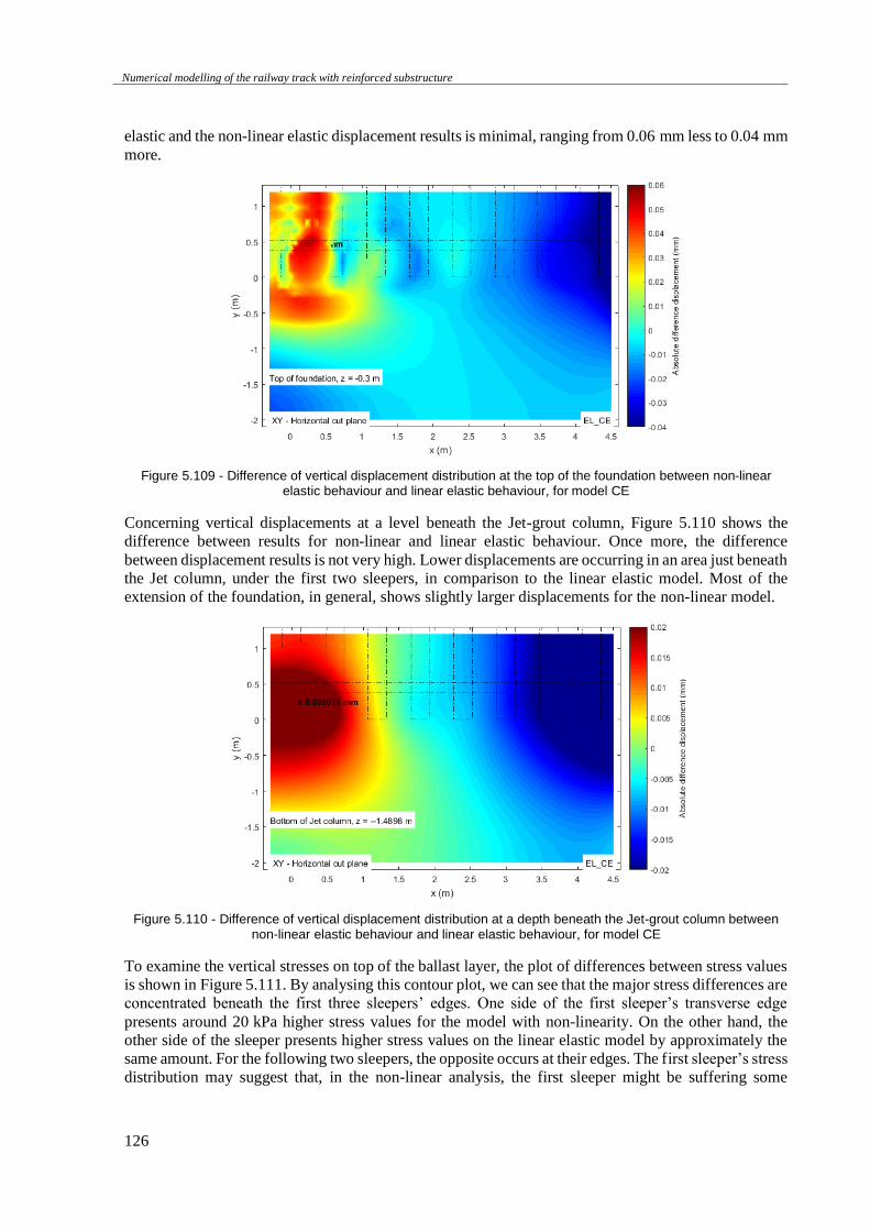
Numerical modelling of the railway track with reinforced substructure
126
elastic and the non-linear elastic displacement results is minimal, ranging from 0.06 mm less to 0.04 mm
more.
Figure 5.109 - Difference of vertical displacement distribution at the top of the foundation between non-linear elastic behaviour and linear elastic behaviour, for model CE
Concerning vertical displacements at a level beneath the Jet-grout column, Figure 5.110 shows the
difference between results for non-linear and linear elastic behaviour. Once more, the difference
between displacement results is not very high. Lower displacements are occurring in an area just beneath
the Jet column, under the first two sleepers, in comparison to the linear elastic model. Most of the
extension of the foundation, in general, shows slightly larger displacements for the non-linear model.
Figure 5.110 - Difference of vertical displacement distribution at a depth beneath the Jet-grout column between non-linear elastic behaviour and linear elastic behaviour, for model CE
To examine the vertical stresses on top of the ballast layer, the plot of differences between stress values
is shown in Figure 5.111. By analysing this contour plot, we can see that the major stress differences are
concentrated beneath the first three sleepers’ edges. One side of the first sleeper’s transverse edge
presents around 20 kPa higher stress values for the model with non-linearity. On the other hand, the
other side of the sleeper presents higher stress values on the linear elastic model by approximately the
same amount. For the following two sleepers, the opposite occurs at their edges. The first sleeper’s stress
distribution may suggest that, in the non-linear analysis, the first sleeper might be suffering some
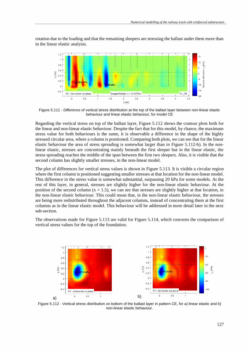
Numerical modelling of the railway track with reinforced substructure
127
rotation due to the loading and that the remaining sleepers are stressing the ballast under them more than
in the linear elastic analysis.
Figure 5.111 - Difference of vertical stress distribution at the top of the ballast layer between non-linear elastic behaviour and linear elastic behaviour, for model CE
Regarding the vertical stress on top of the ballast layer, Figure 5.112 shows the contour plots both for
the linear and non-linear elastic behaviour. Despite the fact that for this model, by chance, the maximum
stress value for both behaviours is the same, it is observable a difference in the shape of the highly
stressed circular area, where a column is positioned. Comparing both plots, we can see that for the linear
elastic behaviour the area of stress spreading is somewhat larger than in Figure 5.112-b). In the non-
linear elastic, stresses are concentrating mainly beneath the first sleeper but in the linear elastic, the
stress spreading reaches the middle of the span between the first two sleepers. Also, it is visible that the
second column has slightly smaller stresses, in the non-linear model.
The plot of differences for vertical stress values is shown in Figure 5.113. It is visible a circular region
where the first column is positioned suggesting smaller stresses at that location for the non-linear model.
This difference in the stress value is somewhat substantial, surpassing 20 kPa for some models. At the
rest of this layer, in general, stresses are slightly higher for the non-linear elastic behaviour. At the
position of the second column (x = 1.5), we can see that stresses are slightly higher at that location, in
the non-linear elastic behaviour. This could mean that, in the non-linear elastic behaviour, the stresses
are being more redistributed throughout the adjacent columns, instead of concentrating them at the first
columns as in the linear elastic model. This behaviour will be addressed in more detail later in the next
sub-section.
The observations made for Figure 5.113 are valid for Figure 5.114, which concerns the comparison of
vertical stress values for the top of the foundation.
a) b)
Figure 5.112 - Vertical stress distribution on bottom of the ballast layer in pattern CE, for a) linear elastic and b) non-linear elastic behaviour.
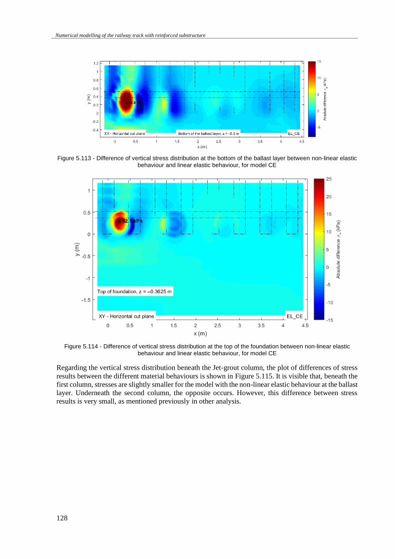
Numerical modelling of the railway track with reinforced substructure
128
Figure 5.113 - Difference of vertical stress distribution at the bottom of the ballast layer between non-linear elastic behaviour and linear elastic behaviour, for model CE
Figure 5.114 - Difference of vertical stress distribution at the top of the foundation between non-linear elastic behaviour and linear elastic behaviour, for model CE
Regarding the vertical stress distribution beneath the Jet-grout column, the plot of differences of stress
results between the different material behaviours is shown in Figure 5.115. It is visible that, beneath the
first column, stresses are slightly smaller for the model with the non-linear elastic behaviour at the ballast
layer. Underneath the second column, the opposite occurs. However, this difference between stress
results is very small, as mentioned previously in other analysis.
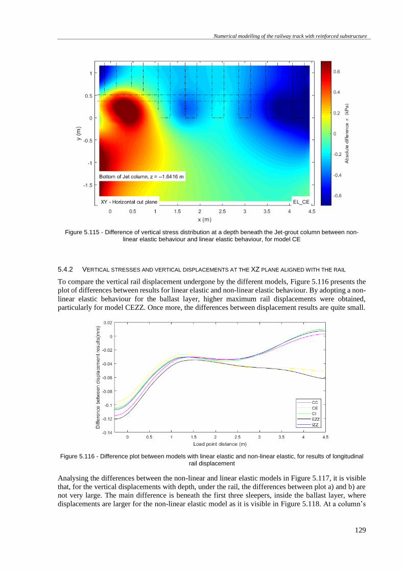
Numerical modelling of the railway track with reinforced substructure
129
Figure 5.115 - Difference of vertical stress distribution at a depth beneath the Jet-grout column between non-linear elastic behaviour and linear elastic behaviour, for model CE
5.4.2 VERTICAL STRESSES AND VERTICAL DISPLACEMENTS AT THE XZ PLANE ALIGNED WITH THE RAIL
To compare the vertical rail displacement undergone by the different models, Figure 5.116 presents the
plot of differences between results for linear elastic and non-linear elastic behaviour. By adopting a non-
linear elastic behaviour for the ballast layer, higher maximum rail displacements were obtained,
particularly for model CEZZ. Once more, the differences between displacement results are quite small.
Figure 5.116 - Difference plot between models with linear elastic and non-linear elastic, for results of longitudinal rail displacement
Analysing the differences between the non-linear and linear elastic models in Figure 5.117, it is visible
that, for the vertical displacements with depth, under the rail, the differences between plot a) and b) are
not very large. The main difference is beneath the first three sleepers, inside the ballast layer, where
displacements are larger for the non-linear elastic model as it is visible in Figure 5.118. At a column’s
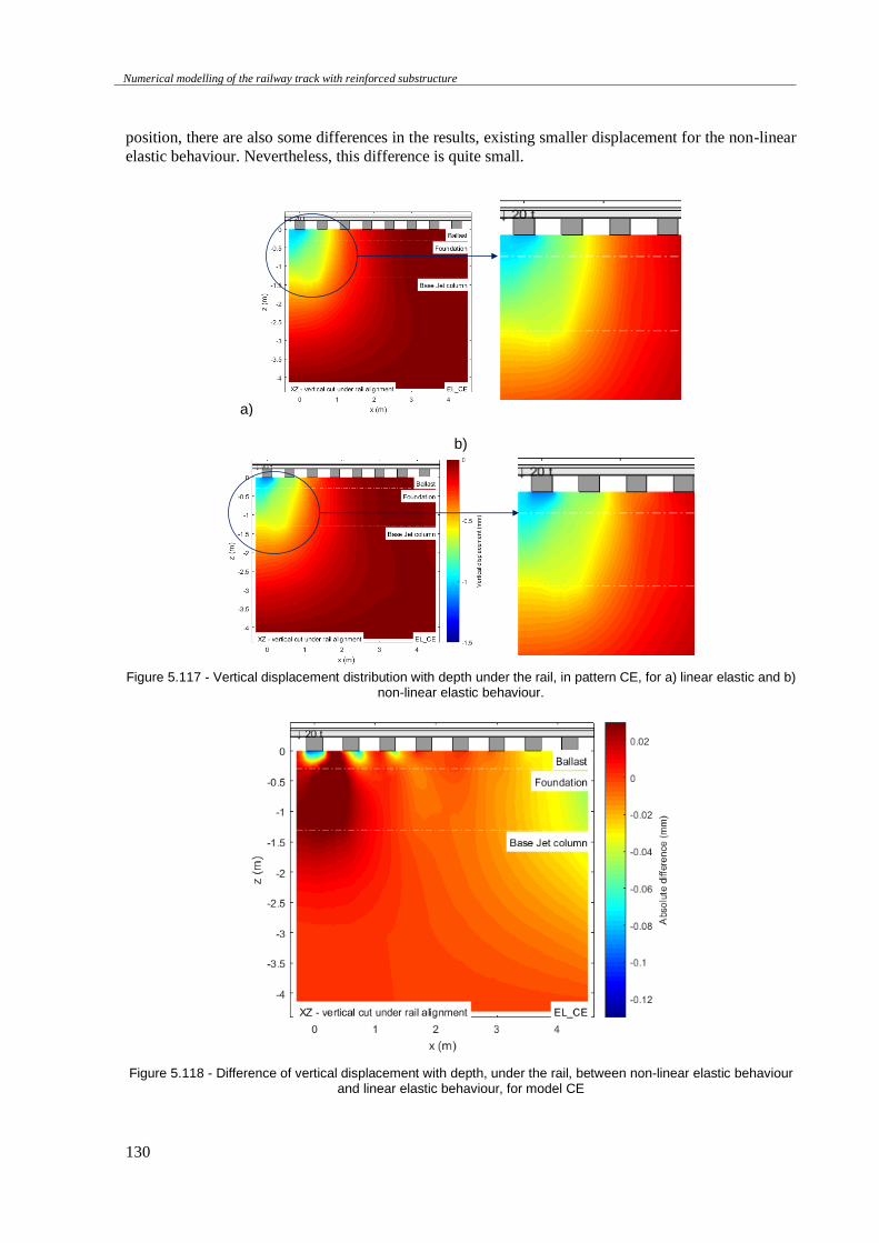
Numerical modelling of the railway track with reinforced substructure
130
position, there are also some differences in the results, existing smaller displacement for the non-linear
elastic behaviour. Nevertheless, this difference is quite small.
a)
b)
Figure 5.117 - Vertical displacement distribution with depth under the rail, in pattern CE, for a) linear elastic and b)
non-linear elastic behaviour.
Figure 5.118 - Difference of vertical displacement with depth, under the rail, between non-linear elastic behaviour and linear elastic behaviour, for model CE
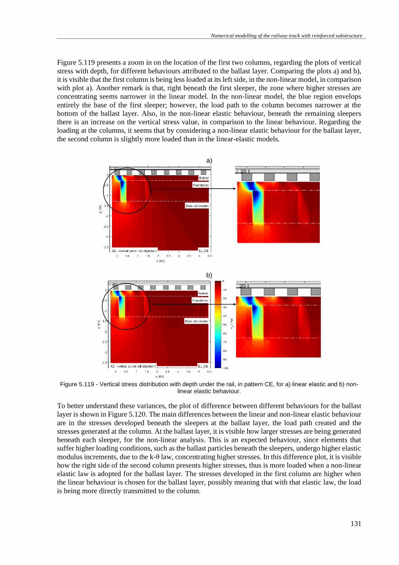
Numerical modelling of the railway track with reinforced substructure
131
Figure 5.119 presents a zoom in on the location of the first two columns, regarding the plots of vertical
stress with depth, for different behaviours attributed to the ballast layer. Comparing the plots a) and b),
it is visible that the first column is being less loaded at its left side, in the non-linear model, in comparison
with plot a). Another remark is that, right beneath the first sleeper, the zone where higher stresses are
concentrating seems narrower in the linear model. In the non-linear model, the blue region envelops
entirely the base of the first sleeper; however, the load path to the column becomes narrower at the
bottom of the ballast layer. Also, in the non-linear elastic behaviour, beneath the remaining sleepers
there is an increase on the vertical stress value, in comparison to the linear behaviour. Regarding the
loading at the columns, it seems that by considering a non-linear elastic behaviour for the ballast layer,
the second column is slightly more loaded than in the linear-elastic models.
a)
b)
Figure 5.119 - Vertical stress distribution with depth under the rail, in pattern CE, for a) linear elastic and b) non-
linear elastic behaviour.
To better understand these variances, the plot of difference between different behaviours for the ballast
layer is shown in Figure 5.120. The main differences between the linear and non-linear elastic behaviour
are in the stresses developed beneath the sleepers at the ballast layer, the load path created and the
stresses generated at the column. At the ballast layer, it is visible how larger stresses are being generated
beneath each sleeper, for the non-linear analysis. This is an expected behaviour, since elements that
suffer higher loading conditions, such as the ballast particles beneath the sleepers, undergo higher elastic
modulus increments, due to the k-θ law, concentrating higher stresses. In this difference plot, it is visible
how the right side of the second column presents higher stresses, thus is more loaded when a non-linear
elastic law is adopted for the ballast layer. The stresses developed in the first column are higher when
the linear behaviour is chosen for the ballast layer, possibly meaning that with that elastic law, the load
is being more directly transmitted to the column.
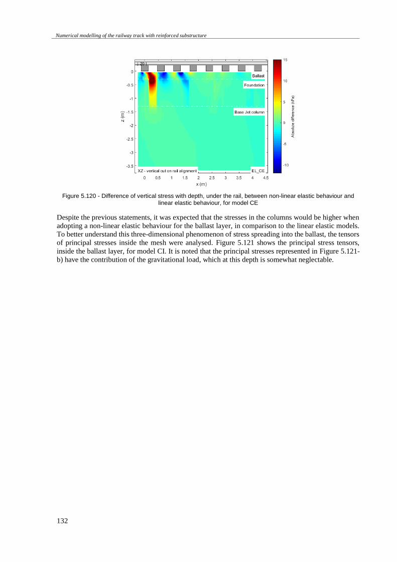
Numerical modelling of the railway track with reinforced substructure
132
Figure 5.120 - Difference of vertical stress with depth, under the rail, between non-linear elastic behaviour and linear elastic behaviour, for model CE
Despite the previous statements, it was expected that the stresses in the columns would be higher when
adopting a non-linear elastic behaviour for the ballast layer, in comparison to the linear elastic models.
To better understand this three-dimensional phenomenon of stress spreading into the ballast, the tensors
of principal stresses inside the mesh were analysed. Figure 5.121 shows the principal stress tensors,
inside the ballast layer, for model CI. It is noted that the principal stresses represented in Figure 5.121-
b) have the contribution of the gravitational load, which at this depth is somewhat neglectable.
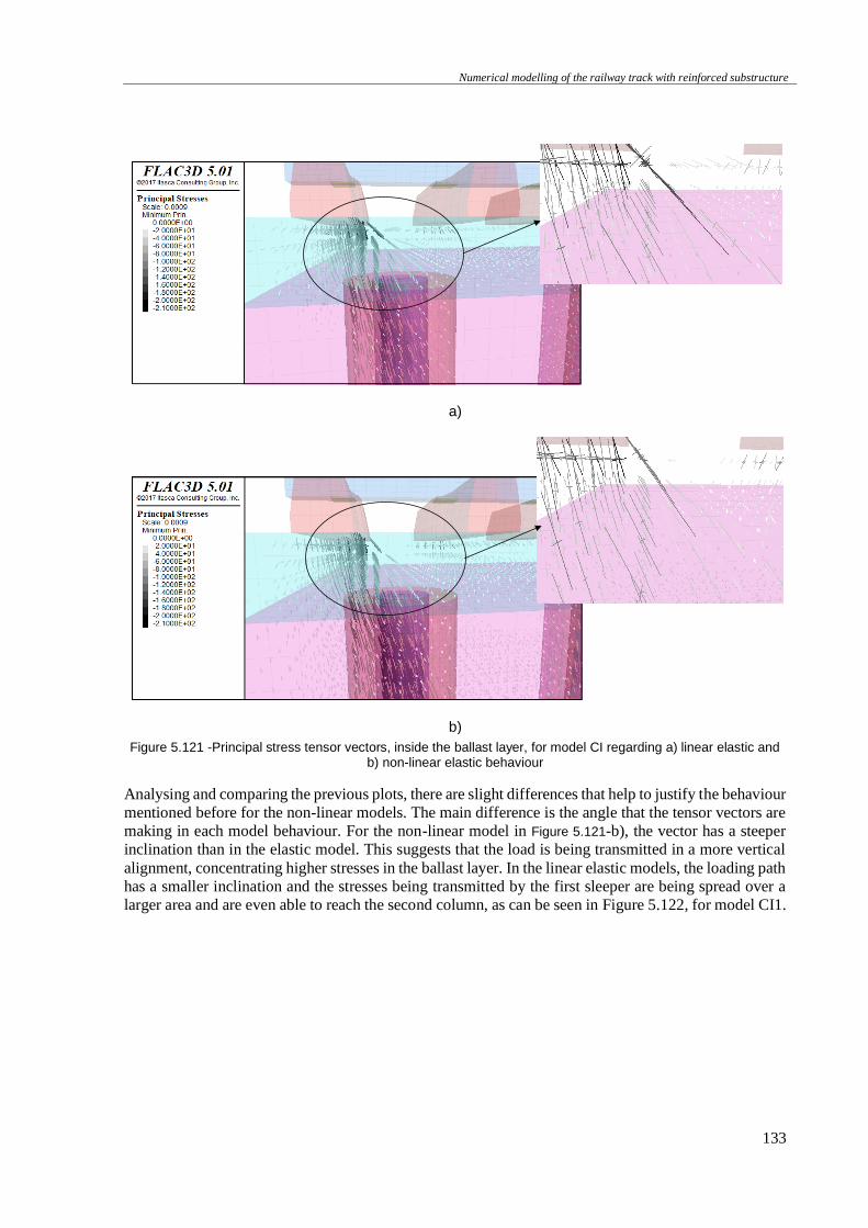
Numerical modelling of the railway track with reinforced substructure
133
a)
b)
Figure 5.121 -Principal stress tensor vectors, inside the ballast layer, for model CI regarding a) linear elastic and b) non-linear elastic behaviour
Analysing and comparing the previous plots, there are slight differences that help to justify the behaviour
mentioned before for the non-linear models. The main difference is the angle that the tensor vectors are
making in each model behaviour. For the non-linear model in Figure 5.121-b), the vector has a steeper
inclination than in the elastic model. This suggests that the load is being transmitted in a more vertical
alignment, concentrating higher stresses in the ballast layer. In the linear elastic models, the loading path
has a smaller inclination and the stresses being transmitted by the first sleeper are being spread over a
larger area and are even able to reach the second column, as can be seen in Figure 5.122, for model CI1.
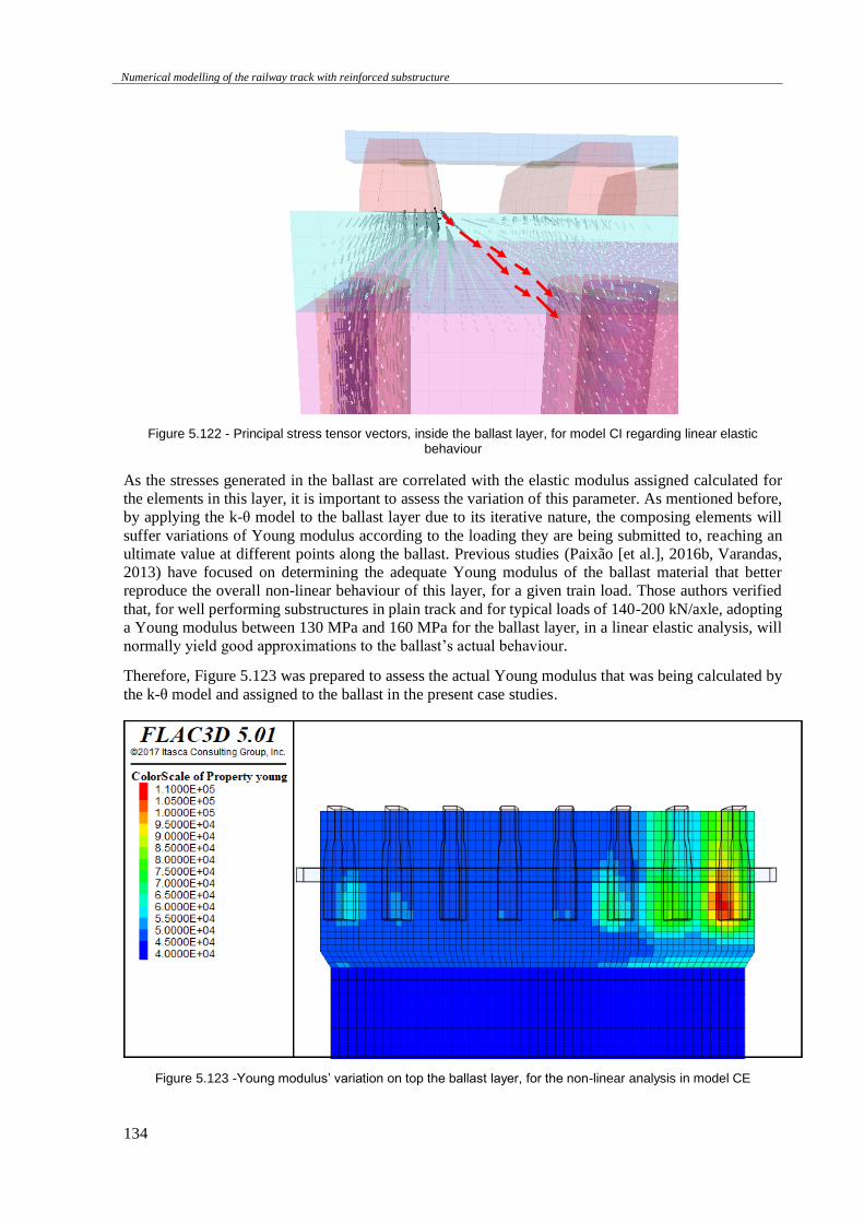
Numerical modelling of the railway track with reinforced substructure
134
Figure 5.122 - Principal stress tensor vectors, inside the ballast layer, for model CI regarding linear elastic behaviour
As the stresses generated in the ballast are correlated with the elastic modulus assigned calculated for
the elements in this layer, it is important to assess the variation of this parameter. As mentioned before,
by applying the k-θ model to the ballast layer due to its iterative nature, the composing elements will
suffer variations of Young modulus according to the loading they are being submitted to, reaching an
ultimate value at different points along the ballast. Previous studies (Paixão [et al.], 2016b, Varandas,
2013) have focused on determining the adequate Young modulus of the ballast material that better
reproduce the overall non-linear behaviour of this layer, for a given train load. Those authors verified
that, for well performing substructures in plain track and for typical loads of 140-200 kN/axle, adopting
a Young modulus between 130 MPa and 160 MPa for the ballast layer, in a linear elastic analysis, will
normally yield good approximations to the ballast’s actual behaviour.
Therefore, Figure 5.123 was prepared to assess the actual Young modulus that was being calculated by
the k-θ model and assigned to the ballast in the present case studies.
Figure 5.123 -Young modulus’ variation on top the ballast layer, for the non-linear analysis in model CE
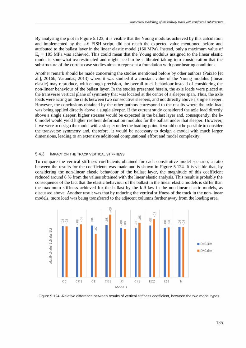
Numerical modelling of the railway track with reinforced substructure
135
By analysing the plot in Figure 5.123, it is visible that the Young modulus achieved by this calculation
and implemented by the k-θ FISH script, did not reach the expected value mentioned before and
attributed to the ballast layer in the linear elastic model (160 MPa). Instead, only a maximum value of
Er = 105 MPa was achieved. This could mean that the Young modulus assigned to the linear elastic
model is somewhat overestimated and might need to be calibrated taking into consideration that the
substructure of the current case studies aims to represent a foundation with poor bearing conditions.
Another remark should be made concerning the studies mentioned before by other authors (Paixão [et
al.], 2016b, Varandas, 2013) where it was studied if a constant value of the Young modulus (linear
elastic) may reproduce, with enough precision, the overall track behaviour instead of considering the
non-linear behaviour of the ballast layer. In the studies presented herein, the axle loads were placed at
the transverse vertical plane of symmetry that was located at the centre of a sleeper span. Thus, the axle
loads were acting on the rails between two consecutive sleepers, and not directly above a single sleeper.
However, the conclusions obtained by the other authors correspond to the results where the axle load
was being applied directly above a single sleeper. If the current study considered the axle load directly
above a single sleeper, higher stresses would be expected in the ballast layer and, consequently, the k-
θ model would yield higher resilient deformation modulus for the ballast under that sleeper. However,
if we were to design the model with a sleeper under the loading point, it would not be possible to consider
the transverse symmetry and, therefore, it would be necessary to design a model with much larger
dimensions, leading to an extensive additional computational effort and model complexity.
5.4.3 IMPACT ON THE TRACK VERTICAL STIFFNESS
To compare the vertical stiffness coefficients obtained for each constitutive model scenario, a ratio
between the results for the coefficients was made and is shown in Figure 5.124. It is visible that, by
considering the non-linear elastic behaviour of the ballast layer, the magnitude of this coefficient
reduced around 8 % from the values obtained with the linear elastic analysis. This result is probably the
consequence of the fact that the elastic behaviour of the ballast in the linear elastic models is stiffer than
the maximum stiffness achieved for the ballast by the k-θ law in the non-linear elastic models, as
discussed above. Another result was that by reducing the vertical stiffness of the track in the non-linear
models, more load was being transferred to the adjacent columns further away from the loading area.
Figure 5.124 -Relative difference between results of vertical stiffness coefficient, between the two model types
-.0
8
-.0
8
-.0
8
-.0
8
-.0
8
-.0
8 -.0
8
-.0
8
-.0
8
-.0
8 -.0
8
-.0
7
-.0
9
-.0
8
-.0
8 -.0
9
-.0
8
-.0
8
C C C C 1 C E C E 1 C I C I 1 E Z Z I Z Z N
ab
s(N
L)-a
bs(E
L)/a
bs(E
L)
Models
D=0.3m
D=0.6m

Numerical modelling of the railway track with reinforced substructure
136
Numerical modelling of the railway track with reinforced substructure
137
6 CONCLUSIONS AND FUTURE
DEVELOPMENTS
This closing chapter seeks to present the major conclusions attained in this study and to suggest future
developments and research, considering the observations made throughout this analysis.
The present work focused on the elaboration of parametric studies regarding the improvement of the
railway track’s subgrade resorting to Jet-grout columns, laying them out in various patterns. The scope
of this study was the railway’s response to such intervention, in what regards stresses and displacements
generated by a static train load. The numerical modelling in these studies was made with a finite-
difference method (FDM) software - FLAC3D - and the post-processing and analysis of results was
carried out with MATLAB.
6.1 MAIN CONCLUSIONS
Due to the subgrade’s importance in the overall track behaviour it is very important to properly design
it, to perform inspection and maintenance operations and, when necessary, to intervene with appropriate
technologies, when track performance is below the expected. Railway track substructure reinforcement
with Jet-grout columns is one of many possible ways to intervene and improve the subgrade
performance. Since those track operations are very costly, time consuming and disrupt normal railway
operation, it becomes imperative to verify their effectiveness. For that purpose, numerical software that
use continuous element methods, like FEM or FDM software, are very appropriate tools that allow to
simulate, with enough accuracy, various aspects of the structural behaviour before and after such
geotechnical interventions.
Since the railway is made up of various elements, when modelling such system, it is essential that all
elements are modelled correctly and that the interconnection between the various elements is represented
properly. Modelling the track system using continuous element methods entails a compromise between
generating a very refined mesh and calculation time (computational effort). Thus, it is necessary to
generate an adequate mesh that can yield results as precise as required for the given problem. In some
situations, for example due to the geometric complexity of the structures under analysis, it may be
advantageous to apply specific numerical techniques to merge different mesh layouts. The numerical
modelling studies presented in this thesis, focusing on railway track substructure reinforcement using
different column patterns, is one of those situations. In Chapter 3, a series of parametric studies were
made comprising FLAC3D commands “ATTACH” and “INTERFACE” that are used to adjoin different
mesh types, allowing a deeper insight on how to implement these commands.
The first parametric study allowed to draw conclusions concerning the assignment of the nature of an
interface, that depends on the stiffness of the adjacent materials, calculated by Eq. (1), according to the
Numerical modelling of the railway track with reinforced substructure
138
software’s manual. If an interface has two similar materials adjoining it, choosing between a stiff or soft
behaviour interface is almost irrelevant, being advised to opt for an interface behaviour based in the
stiffer material adjacent to the interface. Nevertheless, if the properties of those adjacent materials differ
significantly, as proposed in the software manual, soft interface behaviour should be chosen, to avoid
significantly increasing computational effort and calculation times.
The second parametric study had the purpose to compare and distinguish the commands mentioned
above, when applied to adjoin distinct types of sub-grids. Results suggested that choosing between the
“ATTACH” or “INTERFACE” command will not affect results considerably, suggesting that the
application of the “ATTACH” command is satisfactory and more efficient, in terms of calculation effort.
Weighing both commands, if no slip or separation is expected at the location where an interface might
be placed, it is prudent to choose the “ATTACH” command due to its easier implementation comparing
with the “INTERFACE” command, that involves complicated geometric generation and assignment of
interface attributes. These parametric studies were made to better understand how to apply these tools
when designing a complex model of the railway track system.
Later on, a parametric study on the structural behaviour of the railway track with reinforced substructure
was made. The complex model studied was designed as mentioned in Chapter 4, where two types of
behaviours were adopted for the ballast layer: i) linear elastic and ii) non-linear elastic using the k-θ
model (Brown & Pell, 1967). It was analysed the influence of the Jet-grout column’s diameter, column
placement and loading position.
In general, both material behaviours yielded comparable results in what concerns the reinforced track’s
behaviour. However, some differences were found.
When analysing the influence of the column’s diameter size, it was seen that, in general, by increasing
the column’s diameter smaller displacements are obtained for the top of the ballast and foundation and
higher displacements occur beneath the Jet column. However, the improvement obtained, displacement-
wise, was not very significant when increasing the column’s diameter.
Concerning vertical stresses, results demonstrated that an increase in column size leads to higher stress
concentrations at the ballast layer, beneath the sleepers. At the foundation level, when a smaller diameter
was adopted, higher stress concentrations would occur at a column’s position, whereas, with a larger
diameter smaller stresses would arise, since there is a larger area for stress spreading. Beneath the Jet-
grout columns, higher stresses would develop under the column, for the larger diameter, which could
mean that a pressure bulb was created under it. With a larger column diameter, larger pressure bulbs are
created as it was seen in these results.
The results of the rail’s vertical displacement demonstrated that an increase of the columns radius led to
a reduction of the rail’s displacement, having the models where the columns are placed closer to the rail
a slight better performance.
In the XZ vertical plane, it was observed that with a larger radius, vertical deflections underneath the
first sleeper are reduced and that the columns placed in the foundation, might undergo some differential
settlements. Regarding vertical stress with depth, it was visible a clear stress path from the bottom of
the sleepers to the column, where possibly stresses are being more efficiently directed to with a larger
column diameter.
In what regards the influence of reinforcing the substructure, an analysis of the vertical displacements
results showed that, in general, with an improved substructure, slightly smaller displacements are
obtained under the first sleeper extending till the third sleeper, at the top of the ballast and foundation.
At the bottom of the columns, displacements of the improved substructure at that level are roughly
higher than the non-improved model. In general, as expected, the reinforced structures under study
showed slightly lower vertical displacements assessed at the rail level, having the external column
layouts reinforcement showed a better performance.
Numerical modelling of the railway track with reinforced substructure
139
By analysing the vertical stress results, at the positions where a column is placed, higher stresses are
developed at the ballast layer and foundation, possibly due to the presence of the stiffer substructure
which directs stresses into that region, creating a clear loading path.
By installing Jet-grout columns in the foundation, the stresses being developed by the train load with
depth, instead of spreading evenly throughout the foundation, are being concentrated in limited zones
of stiffer nature, being a stress path created from the base of the sleepers to the column. In the XZ plane,
lower vertical displacements are observed under the first sleeper however, not so significant.
What regards the influence of the axle load position, with the contour plots it was possible to perceive
that displacements are smaller and stresses higher when a column is present beneath the loading point,
as expected. By querying vertical stress results at pertinent positions of the track, it was demonstrated
that, by applying Jet columns to the substructure, there is a stress reduction in the substructure
surrounding the column, in comparison with the original stresses, being most of the load induced stresses
now directed to the columns, relieving the surrounding ground.
In terms of vertical stiffness coefficient, with the improved substructure and diameter increase, the track
stiffness increased. Column patterns placed externally to the rail showed the highest increase in vertical
stiffness. With the diameter increase, the coefficient’s value increased constantly, independently of the
layout used, except for the CC model.
In general, the main differences between the linear elastic and the non-linear elastic model lay in the
stress values, since the consideration of the linear-elastic behaviour for the ballast layer somewhat
reproduced the global track behaviour, analysed in terms of vertical displacements.
At the top of the ballast layer, displacements under the first three sleepers are higher, for the non-linear
behaviour of the ballast layer. On top of the foundation, the k-θ model presented smaller displacements
where columns were placed, in comparison to the linear elastic. Beneath the Jet columns, vertical
displacements are smaller for the non-linear behaviour, meaning that the columns suffer smaller
differential settlements with this analysis. However, these differences mentioned are not very
significant.
Rail vertical displacements were demonstrated to be slightly higher for the non-linear elastic behaviour.
Referring to vertical stresses, it was seen that, for a non-linear elastic behaviour, on top of the ballast
layer, the first sleeper presented some stress differences at its edges suggesting that sleeper rotation is
happening due to the train load. This behaviour was not visible in the linear elastic models. It was also
visible that larger stresses were generated beneath each sleeper, for the non-linear analyses. This was an
expected behaviour since elements that suffer higher loading experience higher elastic modulus
increments, concentrating higher stresses. In general, it was demonstrated that, by opting for a non-linear
behaviour for the ballast layer, higher stresses would accumulate at this level.
At the bottom of the ballast layer and top of the foundation, it was visible that, by considering the non-
linear behaviour for the ballast, a wider stress redistribution over the columns was happening, not
concentrating stresses mainly in the first column, as in the linear elastic models. Despite this, the amount
of stress being directed at each column was smaller, when a non-linear behaviour was adopted for the
ballast layer, occurring higher stresses in the columns with the linear behaviour, possibly meaning that
with the elastic law, the load was being transmitted more directly to the column.
Beneath the Jet-grout columns stress results demonstrated, for a non-linear behaviour, smaller values
beneath the first column and higher beneath the remaining ones, corroborating the statement that the
other columns are being more loaded in the non-linear analysis. An analysis of the results in the XZ
planes also showed that the second column is more loaded in the non-linear analysis.
The results of stress distribuition with depth, under the rail, showed that, for the non-linear analysis, the
load path is narrower. By analysing the stress tensor vectors it was seen that inside the ballast layer,
Numerical modelling of the railway track with reinforced substructure
140
there was a difference in the vectors inclinations, due to different material behaviour. The non-linear
model showed steeper inclination in comparison with the elastic one, meaning that loads were being
trasmitted in a more vertical manner, thus concentrating higher stresses at the ballast layer under the
loading region. It was also visible that the elastic models had the ability of spreading stresses over a
larger area, inclusively, being able to directly load other columns adjacent to the one that was right
bellow the axle load.
The value of the Young modulus assigned to the linear elastic behaviour of the ballast layer was based
in previous studies performed by Paixão [et al.] (2016b) and Varandas (2013). However, when analysing
the actual Young modulus that was being calculated by the k- θ model, it was seen that the achieved
value was quite lower than the one assigned to the ballast layer in the linear elastic approach, meaning
that an overestimation of this parameter was made for this study’s conditions. It should be pointed out
that the studies mentioned above were made considering a well-performing railway track substructure
and that the axle loads were acting in the vertical alignment of a sleeper. This was not case of the studies
presented here, where it was intended to simulate a poor-performing substructure and the axle load was
applied at mid-span between sleepers.
6.2 FUTURE WORKS AND RECOMMENDATIONS
These parametric studies allowed a better understanding of the railway track’s behaviour when its
substructure is improved. However, some suggestions for future developments can be made that might
allow a deeper and better understanding of this ground improvement methodology.
Results demonstrated that the value achieved for the Young modulus in the ballast layer, in non-linear
calculations, was quite lower than the one assigned to the ballast in linear elastic calculations. So, to
achieve more realistic results with the linear elastic approach, it is recommended that a calibration of
the ballast’s Young modulus should be made for linear elastic calculations considering the axle load
position and the poor bearing characteristics of the substructure.
This study was made considering the train load as static, however to achieve more realistic results,
moving and dynamic train loads should be considered in future studies since it has a very high influence
in the stress paths inside the upper layers of the track.
A simplification that was made in this study was the assumption of a perfect bond between the columns
and the foundation soil. However, it might be interesting to introduce interface elements surrounding
the Jet-grout columns, to investigate the interaction forces that may surge when the railway is loaded
and if slip is occurring between the columns and surrounding soil.
Nevertheless, it is recommended that more layout patterns for the columns should be studied, since there
are many possible combinations. With this study, it can be advised to study patterns where columns are
placed in positions closer to the rail.
Numerical modelling of the railway track with reinforced substructure
141
1 REFERENCES
Adam, D.; Vogel, A.; Zimmermann, A. - Ground improvement techniques beneath existing rail tracks. 6th International Conference on Ground Improvement Techniques. Coimbra, Portugal. 18-19 July 2005. (2005).
Adegoke, Clement W.; Chang, Ching S.; Selig, Ernest T. - Study of analytical models for
track support systems. 58th Annual Meeting of the Transportation Research Board. Washington District of Columbia, United States. 15-19 January 1979. (1979). p. 12-20.
Allaart, Albert Pieter - Design principles for flexible pavements: a computational model for
granular bases. Technische Universiteit Delft. Delft, (1992). Ph.D. Alves Ribeiro, A.C. - Transições aterro-estrutura em linhas ferroviárias de alta velocidade:
análise experimental e numérica. Faculty of Engineering, University of Porto (FEUP). Porto, (2014). Ph.D.
Arulrajah, A.; Abdullah, A.; Bo, M. W.; Bouazza, A. - Ground improvement techniques for
railway embankments. Proceedings of the Institution of Civil Engineers: Ground Improvement. Vol. 162. n.º 1 (2009). p. 3-14. ISSN: DOI: 10.1680/grim.2009.162.1.3.
Berthelot, P; Pezot, B; Liausu, Ph - Amélioration des sols naturels ou anthropiques par
colonnes semi-rigides: Le procédé CMC. 13th European Conf. on Soil Mechanics and Geotehnical Engineering (XIII ECSMGE). Prague, Czech Republic. (2003). p. 25-29.
Brecciaroli, Fabrizio; Kolisoja, Pauli - Deformation behaviour of railway embankment
materials under repeated loading - Literature review. Helsinki: Finish Rail Admnistration A 5/2006, (2006). ISBN: 952-445-147-6
Broms, B B - Design of lime, lime/cement and cement columns. Keynote lecture.
International Conference on Dry Mix Methods for Deep Soil Stabilization. Stockholm, Sweden 13-15 October 1999. Balkema. (1999). p. 125-153. ISBN:
Numerical modelling of the railway track with reinforced substructure
142
Brown, SF; Pell, PS - An experimental investigation of the stresses, strains and deflections in a layered pavement structure subjected to dynamic loads. Intl Conf Structural Design Asphalt Pavements. Michigan, Ann Arbor. (1967). p. 487-504.
Burrow, MPN; Bowness, D; Ghataora, GS - A comparison of railway track foundation design
methods. Proceedings of the Institution of Mechanical Engineers, Part F: Journal of Rail and Rapid Transit. Vol. 221. n.º 1 (2007). p. 1-12. ISSN: 0954-4097. DOI:
Calon, Nicolas; Robinet, Alain; Mosser, JF; Reiffsteck, Philippe; Guilloux, Alain; Cui, Yu-Jun -
Improvement of railroad platforms by column of soil mixing. 9th WCRR. Lille, France. May 22-26 2011. (2011).
CEN - 12715: Execution of special geotechnical work: Grouting. 2000). ISBN/ISSN: CEN - 14679: Execution of special geotechnical works–Deep Mixing. 2005). ISBN/ISSN: Chang, Ching S; Adegoke, Clement W; Selig, Ernest T - GEOTRACK model for railroad track
performance. Journal of Geotechnical and Geoenvironmental Engineering. Vol. 106. n.º 11 (1980). ISSN: 1090-0241. DOI:
Chrismer, SM; Read, DM - Examining ballast and subgrade conditions. Railway Track and
Struct., AREA. (1994). p. 39-42. ISSN: DOI: Chu, Jian; Varaksin, Serge; Klotz, Ulrich; Mengé, Patrick - Construction processes.
Proceedings of the 17th International Conference on Soil Mechanics and Geotechnical Engineering. Alexandria, Egypt. 5-9 October 2009. (2009). p. 3066-3135.
Correia, A Gomes; Loizos, A. - Evaluation of mechanical properties of unbound granular
materials for pavements and rail tracks. Proceedings of the International Seminar on Geotechnics in Pavement and Railway Design and Construction. Athens, Greece. Millpress. (2004). p. 35-60. ISBN: 90-5966-038-2
Dahlberg, Tore - Railway track dynamics-a survey. Linköping University. (2003). ISSN: DOI: Denies, N; Van Lysebetten, G - General Report Session 4–SOIL MIXING 2–DEEP MIXING.
Proceedings of the International Symposium of ISSMGE-TC211. Recent research, advances & execution aspects of ground improvement works. 31 May-1 June 2012, Brussels, Belgium (2012). ISBN:
EC - Panorama of transport- Statistical overview of transport in the European Union Theme 7
-Transport. Luxembourg: Office for Official Publications of the European Communities, (2003). ISBN: 92-894-4993-4
EC - White Paper on transport :Roadmap to a single European transport area :Towards a
competitive and RESOURCE-EFFICIENT transport system Luxembourg Publications Office of the European Union, (2011). ISBN: 978-92-79-18270-9
EC - EU transport in figures General and regional statistics-Statistical books. Brussels:
2014). ISBN:
Numerical modelling of the railway track with reinforced substructure
143
EC - Key figures on Europe. Luxembourg: Publications Office of the European Union, (2017). ISBN: 978-92-79-63348-5
Ekberg, Anders; Paulsson, Björn - INNOTRACK: concluding technical report. International
Union of Railways (UIC), (2010). ISBN: 2746118505 Esmaeili, Morteza; Hakimpour, Seyed Mehrab - Three Dimensional Numerical Modelling of
Stone Column to Mitigate Liquefaction Potential of Sands. Journal of Seismology and Earthquake Engineering. Vol. 17. n.º 2 (2015). ISSN: DOI:
Esmaeili, Morteza; Zakeri, Jabbar Ali; Babaei, Mohammad - Laboratory and field
investigation of the effect of geogrid-reinforced ballast on railway track lateral resistance. Geotextiles and Geomembranes. Vol. 45. n.º 2 (2017). p. 23-33. ISSN: 0266-1144. DOI: http://dx.doi.org/10.1016/j.geotexmem.2016.11.003.
Essler, R - Application of Ground Improvement: Jet Grouting. ISSMGE TC211. International
Society for Soil Mechanics and Geotechnical EngineeringApplication of Ground Improvement: Jet Grouting.-(2008).
Essler, R; Kitazume, M - Application of Ground Improvement: Deep Mixing. ISSMGE TC211
International Society for Soil Mechanics and Geotechnical EngineeringApplication of Ground Improvement: Deep Mixing.-(2008).
Fatahi, Behzad; Khabbaz, Hadi - Optimising The Pattern Of Semi-Rigid Columns To Improve
Performance Of Rail Tracks Overlying Soft Soil Formation. Australian Geomechanics Journal. Vol. 48. n.º 3 (2013). p. 89-97. ISSN: 0818-9110. DOI:
Fatahi, Behzad; Khabbaz, Hadi; Liem Ho, Huu - Effects of geotextiles on drainage
performance of ballasted rail tracks. Australian Geomechanics. Vol. 46. n.º 4 (2011). p. 91-102. ISSN: 0818-9110. DOI:
Fortunato, Eduardo - Renovação de Plataformas Rodoviárias. Estudos relativos à
capacidade de carga. Universidade do Porto. (2005). Ph.D. Fortunato, Eduardo; Paixão, André - Novas soluções de superestrutura de via para Alta
Velocidade Ferroviária. Lisboa: LNEC, (2009). ISBN/ISSN: 978-972-49-2173-0. Fortunato, Eduardo; Resende, Ricardo - Mechanical behaviour of railway track structure and
foundation-Three dimensional numerical modelling. Proc. of RailFound 06 - International Conference on Railway Track Foundations. Birmingham, UK. 11-13 September 2006. University of Birmingham Press. (2006). p. 217-227. ISBN: 0704426005
HaywardBakerInc. - Jet Grouting. Keller Worlwide, (2011). ISBN/ISSN: Huang, Yang Hsien - Pavement analysis and design. 2nd. Englewood Cliffs, NJ: Pearson
Prentice Hall, (1993). ISBN: 0-13-142473- 4 Hughes-Hallet, Deborah; McCallum, William G; Gleason, Andrew M - Calculus:Single and
Multivariable. 6. John Wiley & Sons., (2013). ISBN: 978-0470-88861-2
Numerical modelling of the railway track with reinforced substructure
144
INNOTRACK - D 2.2.1 State of the art report on soil improvement methods and experience. D 2.2.1 State of the art report on soil improvement methods and experience.-(2008).
INNOTRACK - D 2.2.5 Subgrade reinforcement with columns. Part 1 Vertical columns, Part 2
Inclined columns. D 2.2.5 Subgrade reinforcement with columns. Part 1 Vertical columns, Part 2 Inclined columns.-(2009).
Itasca - FLAC 3D: User Manual. Minneapolis, MN, USA: Itasca Consulting Group, (2015).
ISBN/ISSN: Jardine, RJ - Some observations on the kinematic nature of soil stiffness. Soils and
foundations. Vol. 32. n.º 2 (1992). p. 111-124. ISSN: 0385-1621. DOI: Jenck, Orianne; Dias, Daniel; Kastner, Richard - Three-dimensional numerical modeling of a
piled embankment. International Journal of Geomechanics. Vol. 9. n.º 3 (2009). p. 102-112. ISSN: 1532-3641. DOI:
Jianmin, Z - Modelling and optimizing track maintenance and renewal. University of
Birmingham. (2007). Ph.D. Kempfert, Hans-Georg; Raithel, Marc - Chapter 21 - Soil Improvement and Foundation
Systems with Encased Columns and Reinforced Bearing Layers -Ground Improvement Case Histories. San Diego: Butterworth-Heinemann, 2015. - Chapter 21 - Soil Improvement and Foundation Systems with Encased Columns and Reinforced Bearing Layers ISBN: 978-0-08-100698-6.
Koch, E; Szepesházi, R - Laboratory tests and numerical modeling for embankment
foundation on soft chalky silt using deep-mixing. Proc. of the 18 th Intern. Conf. on Soil Mechanics and Geotechnical Engineering.–Paris. (2013). p. 2521-2524. ISBN:
Koerner, Robert M - Designing with geosynthetics 1. Xlibris Corporation, (2012). ISBN: 978-
1-4628-8290-8 Le Kouby, Alain; Bourgeois, Emmanuel; Rocher-Lacoste, Frédéric - Subgrade improvement
method for existing railway lines–an experimental and numerical study. Electronic Journal of Geotechnical Engineering. Vol. 15. n.º E (2010). p. pp 461-494. ISSN: DOI:
Lekarp, Fredrick; Isacsson, Ulf; Dawson, Andrew - State of the art. I: Resilient response of
unbound aggregates. Journal of transportation engineering. Vol. 126. n.º 1 (2000). p. 66-75. ISSN: 0733-947X. DOI:
Li, Dingqing; Selig, Ernest T - Method for railroad track foundation design. I: Development.
Journal of Geotechnical and Geoenvironmental Engineering. Vol. 124. n.º 4 (1998). p. 316-322. ISSN: 1090-0241. DOI:
Madhavi Latha, G; Rajagopal, K; Krishnaswamy, NR - Experimental and theoretical
investigations on geocell-supported embankments. International Journal of Geomechanics. Vol. 6. n.º 1 (2006). p. 30-35. ISSN: 1532-3641. DOI:
McGown, A; Brown, SF - Applications of reinforced soil for transport infrastructure. Proc. of
the 1st Int. Conference on Transportation, Geotechnics, Nottingham, UK., Advances
Numerical modelling of the railway track with reinforced substructure
145
in Transportation Geotechnics–E. Ellis, HS Yu, G. McDowell, A. Dawson, N. Thom (Eds), CRC Press, Taylor & Francis Group, London. (2008). p. 27-36. ISBN:
Montenegro, Pedro - A methodology for the assessment of the train running safety on
bridges. Faculty of Engineering of University of Porto. Porto, (2015). Ph.D. Moreno, Javier; González, Javier; Santos, Antonio; Cuéllar, Vicente -
SUPERTRACK:Retrofitting of track sections by hydraulic fracture injections. Laboratorio de Geotecnia, CEDEXSUPERTRACK:Retrofitting of track sections by hydraulic fracture injections.-(2005).
Morteza, Esmaeli; Mosayebi, Seyed Ali - Factors affecting jet grouting applicability in
stabilizing loose railway subgrades. Proceedings of the 43rd Symposium on Engineering Geology and Geotechnical Engineering:water, soils and sustainability in the intermountain West. Las Vegas, Nevada, USA. 23-25 March 2011. Engineering Geology and Geotechnical Engineering Symposium ( EGGES ). (2011). p. 87-101. ISBN: 9781622762491
Moseley, Michael P; Kirsch, Klaus - Ground improvement Spon Press, (2004). ISBN:
0203305205 Nimbalkar, Sanjay; Indraratna, Buddhima - Field Assessment of Ballasted Railroads Using
Geosynthetics and Shock Mats. Procedia Engineering. Vol. 143. (2016). p. 1485-1494. ISSN: 1877-7058. DOI: http://dx.doi.org/10.1016/j.proeng.2016.06.175.
Okada, Hiroshi - High-speed railways in China. Japan Railway & Transport Review. n.º 48
(2007). p. 22-29. ISSN: DOI: Paixão, André - Transition zones in railway tracks-An experimental and numerical study on the
structural behaviour. Faculty of Engineering of University of Porto. Porto,Portugal, (2014). Ph.D.
Paixão, André; Fortunato, Eduardo - Análise estrutural de via-férrea com recurso a um
modelo numérico tridimensional. 3as Jornadas Hispano Portuguesas sobre Geotecnia en las Infraestructuras Ferroviarias. Madrid. 25-26 June. (2009).
Paixão, André; Fortunato, Eduardo - Rail track structural analysis using three-dimensional
numerical models. 7th European Conference on Numerical Methods in Geotechnical Engineering (NUMGE2010). Trondheim. 02-04 Jun. 2010. (2010). p. 575-580.
Paixão, André; Fortunato, Eduardo; Calçada, Rui - A numerical study on the influence of
backfill settlements in the train/track interaction at transition zones to railway bridges. Proceedings of the Institution of Mechanical Engineers, Part F: Journal of Rail and Rapid Transit. Vol. 230. n.º 3 (2016a). p. 866-878. ISSN: 0954-4097. DOI:
Paixão, André; Varandas, José N.; Fortunato, Eduardo; Calçada, Rui - Non-Linear Behaviour
of Geomaterials in Railway Tracks under Different Loading Conditions. Procedia Engineering. Vol. 143. (2016b). p. 1128-1135. ISSN: 18777058. DOI: 10.1016/j.proeng.2016.06.147.
Pirapakaran, K.; Sivakugan, N. - Numerical and experimental studies of arching effects within
mine fill slopes. Proceedings of the 6th International Conference on Physical
Numerical modelling of the railway track with reinforced substructure
146
Modelling in Geotechnics - Physical Modelling in Geotechnics - 6th ICPMG '06. Hong Kong. (2006). p. 1519-1525. ISBN: 0415415861
Pires, J.; Phuong, H.T.M.; Dumont, A.G.; Vajdić, M.; Lenart, S.; Oslaković, I. Stipanović -
SMARTRAIL – DEL 3.2 Rehabilitation of Open Tracks and Transition Zones. SMARTRAIL – DEL 3.2 Rehabilitation of Open Tracks and Transition Zones.-(2014).
Poorooshasb, H. B.; Meyerhof, G. G. - Analysis of behavior of stone columns and lime
columns. Computers and Geotechnics. Vol. 20. n.º 1 (1997). p. 47-70. ISSN: 0266-352X. DOI: http://dx.doi.org/10.1016/S0266-352X(96)00013-4.
Potts, David M; Zdravkovic, Lidija; Zdravković, Lidija - Finite element analysis in geotechnical
engineering: application. Thomas Telford, (2001). ISBN: 0727727834 Powrie, W; Yang, LA; Clayton, Chris RI - Stress changes in the ground below ballasted
railway track during train passage. Proceedings of the Institution of Mechanical Engineers, Part F: Journal of Rail and Rapid Transit. Vol. 221. n.º 2 (2007). p. 247-262. ISSN: 0954-4097. DOI:
Prause, Robert H; Kennedy, James C - Parametric study of track response. Parametric study
of track response.-(1977). Priebe, H. J. - The design of vibro replacement. Ground Engineering. Vol. 28. n.º 10 (1995).
p. 31-37. ISSN: 0017-4653. DOI: Profillidis, Vassilios A - Railway engineering. Ashgate, (2000). ISBN: 9780754612797 Raju, V.R. - Ground improvement techniques for railway embankments. Railtech
Conference. (2003). ISBN: Ribeiro, Ana - Técnica de tratamento de solos–Jet Grouting. Universidade Técnica de
Lisboa. (2010). MSc Ribeiro, Viviana - Estudos sobre métodos não destrutivos de caracterização do
comportamento dinâmico da viaférrea com diversos tipos de fundação. Faculty of Engineering of Univeristy of Porto. Porto, (2015). MSc
Selig, E. T.; Waters, J. M. - Track geotechnology and substructure management. London:
Thomas Telford Publications, (1994). ISBN: 0727720139 Stewart, Harry - The prediction of track performance under dynamic traffic loading. University
of Massachusetts Amherst. (1982). Ph.D. Sunaga, Makoto; Hifumi, AOKI - Development of slab tracks for Hokuriku Shinkansen line.
Quarterly Report of RTRI. Vol. 42. n.º 1 (2001). p. 35-41. ISSN: 0033-9008. DOI: Taciroglu, Ertugrul - Constitutive modeling of the resilient response of granular solids.
University of Illinois at Urbana-Champaign. Urbana, Illinois, (1998). Ph.D. Tarabji, SD; Thompson, MR - PROGRAM ILLI-TRACK: Finite Element Analysis of a Railway
Track Support System,User’s Manual. PROGRAM ILLI-TRACK: Finite Element Analysis of a Railway Track Support System,User’s Manual.-(1976).
Numerical modelling of the railway track with reinforced substructure
147
Teixeira, Paulo - Contribución a la reducción de los costes de mantenimiento de vías de alta velocidad mediante la opitimización de su rigidez vertical. Universitat Politècnica de Catalunya. (2004). Ph.D.
Townsend, Frank C; Anderson, J Brian - A compendium of ground modification techniques.
Florida Department of Transportation. A compendium of ground modification techniques.-(2004).
UIC - Track-Bed Layers for Railway Lines (UIC Code 719 R). International Union of
Railways, Paris, France. Track-Bed Layers for Railway Lines (UIC Code 719 R).-(2008).
Varandas, J.N. - Long-term behaviour of railway transitions under dynamic loading
application to soft soil sites. Faculdade de Ciências e Tecnologia da Universidade Nova de Lisboa- FCT/UNL. Lisboa, (2013). Ph.D.
Varandas, J.N.; Paixão, André; Fortunato, Eduardo - A study on the dynamic train-track
interaction over cut-fill transitions on buried culverts. Computers & Structures. Vol. 189. (2017). p. 49-61. ISSN: 0045-7949. DOI:
Varandas, J.N.; Paixão, André; Fortunato, Eduardo; Hölscher, Paul - A Numerical Study on
the Stress Changes in the Ballast Due to Train Passages. Procedia Engineering. Vol. 143. (2016). p. 1169-1176. ISSN: 18777058. DOI: 10.1016/j.proeng.2016.06.127.
Varandas, J.N.; Paixão, André; Fortunato, Eduardo; Hölscher, Paul; Calçada, Rui -
Numerical modelling of railway bridge approaches: influence of soil non-linearity. The Int. J. of Railway Technology. Vol. 3. n.º 4 (2014). p. 73-95. ISSN: DOI:
Wu, Jiu-Jiang; Li, Yan; Cheng, Qian-Gong; Wen, Hua; Liang, Xin - A simplified method for
the determination of vertically loaded pile-soil interface parameters in layered soil based on FLAC3D. Frontiers of Structural and Civil Engineering. Vol. 10. n.º 1 (2016). p. 103-111. ISSN: 2095-2449. DOI: 10.1007/s11709-015-0328-4.
Zeghal, Morched - Discrete-element method investigation of the resilient behavior of granular materials. Journal of Transportation Engineering. Vol. 130. n.º 4 (2004). p. 503-509. ISSN: 0733-947X. DOI:

Numerical modelling of the railway track with reinforced substructure
148