Numerical model for determining fire behaviour of structures

Građevinar 1/2012

1

Neno Torić, Alen Harapin, Ivica Boko

Numerical model for determining fire behaviour of structures

A numerical model and computer program for predicting behaviour of structures subjected to fire action are presented in the paper. The nonlinear numerical procedure is conducted in pre-defined time increments. At that, the distribution of temperature is calculated in each increment and, depending on this calculation, material properties and stiffness of the element are corrected, and the static problem is resolved. The efficiency and accuracy of the model and computer program are presented on an example of a simply supported beam.


Numerički model ponašanja konstrukcija uslijed požara

U radu je prikazan numerički model i razvijeni računalni program za predviđanje ponašanja konstrukcija uslijed djelovanja požara. Nelinearni numerički postupak provodi se u zadanim vremenskim inkrementima, pri čemu se u svakom inkrementu proračunava razdioba temperature, u ovisnosti o njoj korigiraju karakteristike materijala i krutost elementa te rješava statički problem. Na jednostavnom primjeru čeličnog grednog nosača prikazana je efikasnost i točnost razvijenog modela i računalnog programa.


Numerisches Modell des Verhaltens von Konstruktionen infolge einer Brandwirkung

In der Arbeit ist das numerische Modell und das entwickelte Computerprogramm zur Prognosierung des Verhaltens von Konstruktionen infolge einer Brandwirkung dargestellt. Das nichtlineare numerische Verfahren wird innerhalb der vorgegebenen Zeitinkremente durchgeführt, wobei in jedem Inkrement die Temperaturverteilung ausgerechnet wird und abhängig davon werden die materiellen Charakteristiken und die Festigkeit der Elemente korrigiert sowie das statische Problem gelöst. Anhand des einfachen Beispiels des Einfeldträgers werden Effizienz sowie die Genauigkeit des entwickelten Modells und Computerprogrammes dargestellt.

GRAĐEVINAR 64 (2012) 1, 1-13

UDK 624.044+624.92:699.81

Neno Torić, B.Sc. CE

University of Split

Faculty of Civil Engineering, Architecture and Geodesy

[email protected]

Prof. Alen Harapin, Ph.D. CE

University of Split


[email protected]

Prof. Ivica Boko, Ph.D. CE

University of Split


[email protected]

Ključne riječi:

Key words:

Schlüsselwörter:

požarno opterećenje, mehaničke karakteristike, numerički model, provođenje topline, nelinearni proračun, čelik, beton

fire load, mechanical properties, numerical model, heat transfer, nonlinear analysis, steel, concrete

Brandbelastung, mechanische Charakteristiken, numerisches Modell, Wärmeleitung, nichtlineareBerechnung, Stahl, Beton

Received: 29.9.2011.

Corrected: 21.10.2011.

Accepted: 24.1.2012.

Available online: 15.2.2012.

Autori:

Izvorni znanstveni rad

Original scientific paper

Wissenschaftlicher Originalbeitrag


Građevinar 1/2012

2

(1)

(2)

GRAĐEVINAR 64 (2012) 1, 1-13


1. Introduction

Numerical modelling of behaviour of structures subjected to fire is currently one of topical subjects of vital importance on the global level. The development of simple and efficient numerical models, especially those that have been confirmed through experimental study [1, 2], is the basis for better understanding of fire as a stochastic process, and for further development of construction standards with requirements for better and safer structures.

First scientific studies on the effect of fire on man-made structures were conducted already in 1960s. Since then, development of computers has spurred astonishing advances in all fields of engineering, and hence also fast evolution of mathematical/numerical models for the description of fire action on structures. First models were developed in 1970s, mostly for steel structures, and were based on the hybrid model of nonlinear bearing capacity of cross section, as combined with the heat transfer model. These models most often originated from the 2D heat transfer model that provided sufficiently good predictions about development of temperature in structure, if the structure is uniformly heated along the entire span, which was most often not true in real fire situations.

In more recent studies [3, 4, 5, 6], hybrid models have been complemented and improved with various mechanical structural model formulations based on 1D/2D elements for description of structure/section geometry, which was combined with 3D heat transfer models that enable more accurate prediction of temperature distribution within the structure. The definition of constitutive law of behaviour of materials at high temperatures in case of multiaxial stress still remains a considerable problem in experimental research, especially as it does not enable the use of the 3D mechanical model of cross section. The prediction of fire behaviour of structures is more accurate in case of steel structures when compared to concrete structures. This is due to less complicated behaviour of steel at high temperatures, and also to smaller deviation of experimentally defined mechanical properties of steel [7]. The prediction of fire behaviour and fire resistance of structures has become more accurate after introduction of various implicit and explicit material creep models defining creep effect at high temperatures [8, 9].

2. Description of the numerical model

2.1. Introduction

The numerical model that accurately depicts behaviour of structures under fire must be capable of describing, in addition to nonlinear behaviour of structures subjected to load, the development of temperature within the structure and the change of material properties at high temperatures.In order to conduct such a complete (nonlinear) analysis, it

is of high significance to know the cross-sectional geometry, the exact type and position of reinforcement (for reinforced-concrete structures), load conditions, and the constitutive material law, which is generally nonlinear.The results of this analysis can greatly alter the stress and strain situation in individual structural elements, and enable structural engineer to gain a better insight into the behaviour and possible bearing capacity failure, which ultimately leads towards construction of more durable and economical structures.

2.2. Linear elastic model for beam elements

The principal starting point of almost all nonlinear analyses is the linear analysis, i.e. the analysis of materials conforming to Hooke's law. As this numerical model for behaviour of beam-element structures is very well known, and as it has often been described in the literature [10, 11, 12], it will only be briefly outlined in this study.

Two-node, rectilinear, ideally straight and partly prismatic final elements, with 6 degrees of freedom per node, considered so far in many papers [11, 13, 14, 15, 16, 17], are used in this paper.Behaviour of a beam element under load can generally be described using the following linear differential equation of equilibrium:

Where: - internal force vector - bracing vector - load vector - differential operator

In the absence of analytical solutions, the solution to equation (1) is normally sought through numerical procedures. One of the most often used and widely recognized procedures is the finite element method. The basic idea behind this method is to replace the system having an indefinite number of degrees of freedom with the system having a finite number of degrees of freedom. To achieve this, the behaviour of a set of points within a system is assumed (programmed) on a single finite element, as related to a specified number of fixed, previously determined points (nodes) on the same element.An approximate solution of the displacement field on a single element is assumed as follows:

where H is the basic function matrix, while is the vector of unknown node displacements. In case of beam-element systems, basic (shaping) functions are most frequently selected for the Hermite polynomial group [11, 13].

Građevinar 1/2012

3

The following can be deduced from the external and internal force equivalence:

that is:

i.e. after the left side is multiplied with :

or more simply:

where: - vector of internal forces at the ends of the finite element - element stiffness matrix - vector of external forces

GRAĐEVINAR 64 (2012) 1, 1-13


Local stiffness matrices and load vector must be transformed to the global coordinate system and, after transformation, the global system equilibrium is established by simple arrangement of stiffnesses and fixity forces in the corresponding nodes of the finite element mesh.

These are generally known equations where K and F are matrices of stiffness and load, respectively, while u is the global displacement vector.Before solving the above equation system, it is necessary to insert boundary conditions which, in case of a static problem, represent specified forces and/or displacements at system edges.

Prior to transformation to the global coordinate system, the local stiffness matrix of an element can be expressed, in its explicit form, as:

(3)

(4)

(5)

(6)

(7)

(8)

Građevinar 1/2012

4 GRAĐEVINAR 64 (2012) 1, 1-13


It can clearly be seen from the above expression (8) that the local stiffness matrix, apart from depending on the beam length l , also depends on the material parameters: E, G, and the geometrical parameters: A, Iy and Iz. In case of a real element (beam/column) subjected to a load, internal forces (and primarily bending and torsion moments)

Figure 1 . Stress-strain and stiffness along the girder as related to the level of stress in cross-section

can in a nonlinear case significantly alter distribution of stress and strain, which causes the change in stiffness.The material nonlinear analysis can very easily be applied by dividing the element into smaller parts (subelements), in which case the real stiffness is calculated for each subelement (Figure 1).

Građevinar 1/2012

5GRAĐEVINAR 64 (2012) 1, 1-13


In order to conduct the nonlinear analysis, it is therefore necessary to define in which way the cross sectional stiffness at various levels of stress should be calculated.

2.3. Calculation of stress and strain and calculation of cross-sectional stiffness

2.3.1. Basic assumptions

Basic premises of the model for calculating stress-strain situation along the cross-section [12, 18, 19] are:

- cross-sections remain flat even after deformation,- no sliding has been occurred at the connection of different

materials,- uniaxial stress-deformation relationship (constitutive law) is

known for all materials.

2.3.2. Cross-section deformation plane

The graphical view of a possible deformation plane, as compared to the previous state of equilibrium, is presented in Figure 2. An additional deformation of a given cross-sectional point is defined through equation of a plane:

where:

In the above expressions represents the vector of unknown parameters of the additional strain plane, and y, z the coordinates of the point in the Y-Z plane. The strain plane is described by its intersection with the X coordinate axis, and the components of relative rotations , around the Z and Y axis, respectively. If the considered section point has previous strain , its total strain is:

The deformation is known and determined through equilibrium position via , by analogy to expression (9), by means of:

If expressions (9) and (13) are inserted in the expression (12), we get:

or:

where is the vector of the total plane deformation parameters.

Figure 2. Graphical presentation of a possible deformation plane

2.3.3. Relationship between stress and strain

The starting point is the known relationship between the uniaxial stress s and strain e for a given material, i.e. the so called constitutive law of material behaviour. For real materials, this relationship is basically curved, and is defined by uniaxial test or appropriate regulations. From the standpoint of numerical analysis, it is appropriate to define this relationship as linear by individual segments (Figure 3). The controlled error introduced in this way is negligible when compared to other assumptions. The s-e relationship between any of the two i, j points of the diagram is described by the following expression:

If the expression (14) is inserted in (16) and if the following change is made:

then the stress in the sector under study can be described with the following expression:

In the above expressions, the element E denotes the current modulus of elasticity of material (inclination of the straight line in the sector under study), while graphical interpretation can be seen in Figure 3. It should be noted that the stress is constant and defined for the known initial situation and for the assumed current deformation between the points i and j.

(9)

(10)

(11)

(12)

(13)

(14)

(15)

(16)

(17)

(18)

Građevinar 1/2012

6

is a part of the vector of internal forces which is obtained by integration of the stress along the entire area of the composite cross section. Matrix members I represent current mechanical properties of the cross section.The vector Sv is composed of the vector of external forces Svp, which defines the initial deformation plane , and of the additional force vector , which causes the additional deformation plane .

To establish the balance, Sv must be equal to Su, i.e. :

In its developed form, the expression (24) is the system formed of three equations with an unknown vector

2.3.5. Bar reinforcement

After determination of the total deformation of a given steel bar, the procedure continues by defining between which node deformations i, i+1 on the - diagram it is situated. Then the corresponding elastic model E, is defined, along with contribution of current mechanical properties of bar material, by analogy to expression (22), using:

where As denotes the area of the bar. All bars cross-sections are summed up.A part of the internal force vector the bar reinforcement is contributing to be defined by analogy with the expression (21), i.e. by:

In case of bar-based materials, it is more appropriate to define the initial deformation with the discrete value , rather than with parameters of the initial deformation plane .

2.3.6. Larger area materials

The area of material with significantly greater area when compared to the area of the entire cross section, is assigned through convex polygonal elements without voids (finite

GRAĐEVINAR 64 (2012) 1, 1-13


In case of structures exposed to fire action, the stress and strain relationship of a material is highly dependent on temperature. For that reason, the behaviour of materials subjected to high temperatures is usually described as a set of stress - strain curves, each one for a specific temperature. At that, temperatures situated in between the specified ones are obtained by linear interpolation.

2.3.4. Equilibrium equation

The vector of cross-sectional internal resistance forces Su is a function of the resulting deformation plane and the s-e relationship of a specific material. If they are known, the Su can be calculated by integrating stress along the composite section area:

where Nu is the internal longitudinal force, Mzu and Myu are the corresponding moment forces with respect to coordinate axes, W is the area of a specific material, and S summation across all materials m. If (18) is inserted in (19), then:

where:

Figure 3. Possible stress - strain relationship for a material

(19)

(20)

(21)

(22)

(23)

(24)

(25)

(26)

Građevinar 1/2012

7GRAĐEVINAR 64 (2012) 1, 1-13


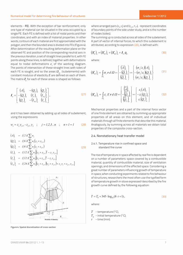
elements - FE). With the exception of bar reinforcement, only one type of material can be situated in the area occupied by a single FE. Each FE is defined with a list of nodal points and their coordinates, and with an index of material properties. In other words, contours of each material are first approximated with the polygon, and then the bounded area is divided into FEs (Figure 4). After determination of the resulting deformation plane on the observed FE and position of the corresponding neutral axis in the previous iteration, a set of straight lines parallel to it, with FE points along these lines, is defined, together with deformations equal to nodal deformations i of the working diagram. The points of intersection of these straight lines with sides of each FE is sought, and so the areas Ωei (subelements) with constant modulus of elasticity E are defined on each of them. The matrix Ie for each of these areas is shaped as follows:

and it has been obtained by adding up all sides of subelement, using the expressions:

Figure 4. Spatial discretisation of cross-section

where arranged pairs ( , ) and ( , ), represent coordinates of boundary points of the side under study, and n is the number of nodes (sides).The summing up is conducted across all sides of the subelement. A part of vector of internal forces, to which this subelement is attributed, according to expression (20), is defined with:

where:

Mechanical properties and a part of the internal force vector of one finite element are obtained by summing up appropriate properties of all areas on this element, and of individual materials through all finite elements that describe this material. Analogously, by summing across all materials we obtain total properties of the composite cross-section.

2.4. Nonstationary heat transfer model

2.4.1. Temperature rise in confined space and standard fire curve

The rise of temperature in space affected by real fire is dependent on a number of parameters: space covered by a combustible material, quantity of combustible material, size of ventilation openings, and dimensions of the affected space. Considering a great number of parameters influencing growth of temperature in space, when conducting experiments related to fire behaviour of structures, researchers the most often use the typified form of temperature growth in stove expressed/described by the fire growth curve defined by the following equation:

where:

T - temperature (°C),T0 - initial temperature (°C),t - time (min).

(27)

(28)

(29)

(30)

(31)

(32)

(33)

Građevinar 1/2012

8

where:- heat flow on the surface of an element (surface heat

flux) (W/m2),- coefficient of convection (W/m2K),- configuration factor,- resulting emissivity factor between the element and fire,- Stephan Boltzmann constant (=5.67A10-8 W/m2K4),- gas temperature near element (°C),- temperature on the surface of the element (°C).

The spatial domain is approximated with a specified number of finite elements, as shown in Figure 5. The presented heat transfer model uses 8-node 3D finite elements.

2.4.3. Integration of discrete system equations

The system of non-linear ordinary differential equations (35) is solved through integration of equations between two neighbouring time points for a relatively small time interval

. Temperatures at the beginning of the time interval are known and are used to calculate temperatures at the end of the time interval, i.e. at the moment t+ . By applying the mixed integration approach to the equation system (35), we obtain:

where: - known temperature at the beginning of the time

interval, - unknown temperature at the end of the time interval,

- interpolation parameter, - field production vector at the end of the time interval, - boundary heat flow vector at the end of the time

interval, - incremental time step.

The iterative procedure for determining the value starts by assuming the equivalence = , in the first iterative step within the time increment . After that, a new temperature value at the end of time interval is calculated, until the following condition is met:

where:

- incremental time step.

GRAĐEVINAR 64 (2012) 1, 1-13


2.4.2. Transient heat transfer

The transient heat transfer is a time-dependant heat transfer process in which the temperature field created by transfer of heat within the area under study changes in time. The model implemented is based on the 3D transient nonlinear heat transfer model. The differential equation describing this process in a spatial setting is defined by the expression:

where:

- density of matter (kg/m3) - specific heat capacity (J/kgK) - thermal conductivity coefficient tensor (W/mK)

- heat diffusion tensor (m2/s)

By applying the weak formulation to the equation (34), and by using the Galerkin method for selection of approximate solution function, we obtain the system of p ordinary differential equations:

where:

- space domain, - edge of space domain, - shape functions for approximate solution,

- total number of nodes in space domain discretisation.

The matrix C is called the capacitive matrix, matrix K the transmission matrix, vector F the thermal load vector, and Q the thermal inflow vector. The heat flow occurring as a result of fire is composed of convection and radiation. The heat flow on the surface of heated element is determined using the following expression:

(34)

(35)

(36)

(37)

(38)

(39)

(40)

(41)

(42)

Građevinar 1/2012

9GRAĐEVINAR 64 (2012) 1, 1-13


Figure 5. a) Global discretization of the space frame. (b) The beam-column element. (c) The element’s cross-section discretization. (d) The comparative body model for heat transfer analysis. (e) The stress-strain constitutive law of the element’s cross-section.

2.5. Integral nonlinear model for estimating behaviour of structures subjected to fire load

The above defined models: model for the analysis of linearly elastic beam-element systems, model for dimensioning composite cross-sections and model for transient heat transfer, have been united into a single integral model: model for analysis of spatial beam-element systems exposed of fire action. The model has been incorporated in a computer program.Figure 6 shows discretisation of a simple structure with the link between the spatial beam-element system, 2D and 3D network. The 2D network is used for discretisation of beam structure cross-sections, i.e. for calculating the stress-strain relationship along cross-section, and for stiffness calculation. The 3D network (model) is used for heat transfer calculation/analysis.The procedure starts by defining the spatial beam (frame) system, i.e. the initial and the final node must be defined for each beam (column/beam). In addition, the cross section with behaviour

pattern ( - diagram) must also be defined for each beam element and for each material used (2D network). The 3D network for heat transfer calculation is then automatically generated along the beam element (beam/column). It is also necessary to define the number of subelements the final element will be divided into. A cross section and the law of behaviour from the global element (beam/column) are attributed to each subelement.The heat flow calculation is made on the global 3D model and an instantaneous temperature is obtained in every node. The mean (average) temperature is calculated at every 2D network element (which represents the cross-section of the element), and the constitutive material law is corrected. After that the stress-strain situation in cross-section can be defined, as well as the cross-section stiffness, which represents stiffness of the beam (beam, column) subelement.The model is incremental and linear along individual increments. The procedure starts from the cross-section level (zero position) by calculating real cross-section stiffness values for unstressed cross-section, according to expressions (22), (25) and (27). The values obtained in this way represent the initial stiffness of cross-section. The initial stiffness values are used to calculate the initial beam-element stiffness matrix. It is significant to note that only axial and flexural properties of cross-section are set/corrected by integration at the cross-section level, while shear and torsional properties are left unchanged. This is followed by the usual procedure of arranging the global stiffness matrix and the global load vector (2), and by system calculation.After calculation of internal forces at the end of the beam element, the position of the deformation plane is determined and new cross-section stiffness is defined. In general, two cases are possible:

1. The deformation plane position can be determined for cross section. In this case, the strength of the cross-section is sufficient to withstand the external force action (i.e. the action of forces obtained by linear analysis of the beam element system).

2. The deformation plane position can not be determined for cross section, i.e. the procedure presented in section 2.2 is divergent. In this case, it can be stated that there is a failure at the cross-section, i.e. that local failure has occurred in the system, and hence that global system failure is also possible. In concrete terms, the stiffness values are then made equal to zero, and the global analysis procedure is reiterated.

The procedure continues until the standard of the displacement increase vector does not fall under an arbitrary value, i.e.:

In all practical cases, it can be assumed that the value amounts to 0.001.The incremental procedure and the computer program flow diagram are presented in Table 1 and Figure 6.

(43)

Građevinar 1/2012

10 GRAĐEVINAR 64 (2012) 1, 1-13


1

The initial load vector, which is actually the nul-vector (F=0) is assumed. On the basis of this load, the initial local stiffness matrices are determined for each beam element (20 and 22), and also the initial global stiffness matrix :

This matrix represents the so called zero stiffness, i.e. the system stiffness not influenced by forces.

2

From the given external load on the beams/columns, defining the forces on elements, and the vector of the applied forces:

3 Time loop, the first time step is set j=1.

4

The calculation of the temperature field in the 3D element (Fig. 5). For each cross section: the calculation of the mean temperature and the correction of the material characteristics according to the calculated mean temperature.

5 iteration loop, the first iteration step is set: i=1.

6

Calculation of node displacement and internal forces on elements:

7

Control of convergence:

If the convergence is satisfied, the procedure is finished and the results are printed. Procedure continues with new time step (4). If the convergence is not satisfied, the procedure continues– step (7).The value is an optionally chosen small value, usually 0,001.

8

The calculation of the new stiffness in 2D elements, according to corrected material characteristics and the corrected internal forces.

Procedure continues with new time step: j=j+1 and the calculation procedure continues to step (6). The procedure continues until certain accuracy is achieved or until divergence occurs. This divergence points out to that load capacity of the cross-section is reached, i.e. the failure of the element in that section and possible failure of the entire structure.

Table 1. Numerical model and incremental procedure

Figure 6. Computer program flow diagram

3. Verification of numerical model

3.1. Description of model and experiment

An example of modelling experiment conducted by Wainman and Kirby [20] is considered in order to present capabilities of the described numerical model for predicting fire behaviour of structures. This experiment involves a freely supported steel element I 254/146, steel quality S275, length: 4.58 m, exposed to temperatures defined by the standard fire curve. A non-composite concrete slab 12.5 cm in thickness and 65 cm in width, situated on top of the element, exerts load amounting to 2.21 kN/m along the length of the slab. Four concentrated forces K were taken as additional load. The forces amount to 32.5 kN and are placed in positions as defined in Figure 7, where we also see disposition of measurement points in which a time-related increase of temperature was monitored.The dimensions and geometrical properties of the steel section I 254/146 that were used as input data for modelling the freely supported steel element are presented in Table 2.

Građevinar 1/2012

11GRAĐEVINAR 64 (2012) 1, 1-13


Figure 7. View of experimental sample [20] with temperature measurement points (W-web, F-flange)

Table 2. Section dimensions and properties

h (mm) b (mm) tw (mm) tf (mm)I (cm4) A

(mm2)Iy Iz

259.6 147.3 7.3 12.7 6558.0 677.0 5452.0

Figure 8 . Stress - strain curves according to Wainman and Kirby

Figure 9. Stress - strain curves according to EN1993-1-2

3.2. Experiment results and comparison with numerical model

Experiment simulation was conducted for two different types of input mechanical properties: experimentally determined stress-strain diagrams for high temperatures [20] corresponding to the quality of steel S275 out of which the element was made, and the stress-strain diagrams given in EN1993-1-2 [21] for engineering calculation of fire behaviour of steel structures, as shown in Figures 8 and 9.

The results obtained in the course of the Wainman and Kirby experiment, and results obtained by model in typical steel element points, are presented in Figures 10-13.

The comparison of results of vertical deflection measured in a half of the element, taken from the experiment conducted by Wainman and Kirby, with results obtained through the described model, is presented in Figure 14.

Građevinar 1/2012

12 GRAĐEVINAR 64 (2012) 1, 1-13


Figure 12. Comparison of temperature results obtained by experiment and model - top flange

Figure 11. Comparison of temperature results obtained by experiment and model - web

Figure 10. Comparison of temperature results obtained by experiment and model - bottom flange

Građevinar 1/2012

13GRAĐEVINAR 64 (2012) 1, 1-13


REFERENCES

Boko, I.; Peroš, B.; Torić, N.: Reliability of steel structures in case of fire, Građevinar 62, 2010., 5, 389-400. (In Croatian)Boko, I.; Peroš, B.: Fire safety of steel structures, Građevinar 54, 2002., 11, 643-656. (In Croatian)Wang, Y. C.; Lennon, T.; Moore, D. B.: The Behaviour of Steel Frames Subject to Fire, Journal of Constructional Steel Research 35, 1995., 291-322.Terro, M. J.: Numerical Modeling of the Behaviour of Concrete Structures in Fire, ACI Structural Journal 95, 1998., 2, 183-193.Elghazouli, A. Y.; Izzuddin, B. A.: Response of Idealized Composite Beam-Slab Systems under Fire Conditions, Journal of Constructional Steel Research 56, 2000., 3, 199-224.Wu B.; Lu, J. Z.: A Numerical Study of the Behaviour of Restrained RC Beams at Elevated Temperatures, Fire Safety Journal 44, 2009., 4, 522-531.Youssef, M. A.; Moftah, M.: General Stress-Strain Relationship for Concrete at Elevated Temperatures, Engineering Structures 29, 2007., 10, 2618-2634.Kodur, V. K. R.; Dwaikat, M. M. S.: Response of Steel Beam-Columns Exposed to Fire, Engineering Structures 31, 2009., 2, 369-379.Dwaikat, M. B.; Kodur, V. K. R.: A Numerical Approach for Modelling the Fire Induced Restraint Effects in Reinforced Concrete Beams, Fire Safety Journal 43, 2008., 4, 298-307.Prezeminiecki, J. S.: Theory of Matrix Structural Analysis, McGrow-Hill, New York, 1968.Bangash, M. J. H.: Concrete, Concrete structures, Numerical Modeling, Applications, Elsevier Applied Science, New York, 1989.

[1]

[2]

[3]

[4]

[5]

[6]

[7]

[8]

[9]

[10]

[11]

Figure 14. Comparison between vertical deflections obtained by experiment and model based predictions

Figure 13. The development of the temperature field in discrete time intervals across the steel element

Radnić, J.; Harapin, A.; Markić R.: Testing influence of ties on the bearing capacity of concrete beams at compressive failure, Građevinar 59 (9) 2007., 789-795. (In Croatian)Mihanović, A.; Marović, P.; Dvornik, J.: Nonlinear calculations of RC structures, DHGK, Zagreb, 1993. (In Croatian)Liew, J. Y. R.; Chen, W. F.; Chen H.: Advanced Inelastic Analysis of Frame Structures, Journal of Constructional Steel Research 55, 2000., 1-3, 245-265.Sapountzakis, E. J.; Mokos, V. G.: 3-D Beam Element of Composite Cross Section Including Warping and Shear Deformation Effects, Computers and Structures 85, 2007., 1-2, 102-116.Yang, Y. B., Kuo, S. R., Wu, Y. S.: Incrementally small-deformation theory for nonlinear analysis of structural frames, Engineering Structures 24, 2002., 6, 783-798.Trogrlić, B.; Mihanović, A.: The Comparative Body Model in Material and Geometric Nonlinear Analysis of Space R/C frames, Engineering Computations 25, 2008., 2, 155-171.Trogrlić, B.; Harapin, A.; Mihanović, A.: The Null Configuration Model in limit load analysis of steel space frames, Materialwissenschaft und Werkstofftechnik 42, 2011., 5, 417–428.Radnić, J.; Harapin, A.: Model for dimensioning of composite cross-sections subjected to bending, Građevinar 45, 1993., 7, 379-389. (In Croatian)Wainman, D. E.; Kirby, B. R.: Compendium of UK Standard Fire Test Data: Unprotected Structural Steel – 1 & 2, British Steel Corporation, 1988.EN 1993-1-2:2005, Eurocode 3 - Design of steel structures - Part 1-2: General Rules - Structural fire design, European Committee for Standardization, Brussels, 2005.

[12]

[13]

[14]

[15]

[16]

[17]

[18]

[19]

[20]

[21]

4. Conclusions

It can be seen from Figures 10-12 that the model predicts, with sufficient accuracy, the temperature increase in typical points of the steel element: at bottom flange, at web, and at top flange. A possible reason why temperatures obtained by model deviate from those obtained by experiment is that the input parameter in the model is the mean temperature of stove, which is defined in a relatively small number of points that do not suffice for accurate description of temperature boundary conditions in experiments. Also, it can be seen from Figure 14 that the model predicts with sufficient precision deflections of the element in the 22 minute time interval, with significant deviation of

deflection at 14 minutes after the start of the experiment, when temperatures of over 450°C are developed in the element, and when the steel creep at elevated temperatures greatly influence deformation of the structure, i.e. deflection of the element.A relatively small deviation in deflection prediction occurs at two different types of stress - strain curves, which points to the fact that the proposed stress - strain curves, based on Eurocode 3 for fire action, are sufficiently accurate for modelling behaviour of steel structures subjected to fire action.Future development of the model will be oriented towards implementation of different implicit and explicit models of steel flow at elevated temperatures, so as to enable a more accurate prediction of element deflection at elevated temperatures.

Documents

Numerical model for determining fire behaviour of structures