Embed Size (px)
Citation preview

Department of BioEngineering College of Engineering
University of Illinois at Chicago
BioE 594 – COMPUTATIONAL METHODS IN BIOMECHANICS Fall 2011
Time & Place: Tuesdays 1:00 P.M. to 3:00 P.M.; ROOM 520 at
New Orthopedic Building, Rush University Medical Center Goals: Computer models are being increasingly used for the solution of many complex problems in biomechanics. This course will give the students an insight on how computer models based on numerical methods are applied in orthopedic biomechanics. Students will be required to complete mini projects in each of the applications that will be discussed in this course. Instructor: Raghu N. Natarajan Ph.D. Professor, Department of Orthopedics, Rush-Presbyterian-St.Luke’s Medical Center and Department of BioEngineering, University of Illinois at Chicago. (e-mail : [email protected]) Topics (1) Introduction to Orthopedics (2) Numerical methods (3) Introduction to Finite Element Method (4) Contact Analysis: Total Knee Replacement & Total Hip Replacement (5) Stress shielding in Total Hip Replacement (6) Micromotion in Orthopedics (7) Effect of surgical interventions on lumbar motion segment (8) Projects Grading: Homework 30% Projects 40% Final comprehensive examination 30%
NUMERICAL METHODS THAT CAN BE USED IN BIOMECHANICS
1) Mechanics of Materials Approach
(A) Complex Beam Theory
(i) Straight Beam
(ii) Curved Beam
(iii) Composite Beam
From:Daviddarling.info

NUMERICAL METHODS THAT CAN BE USED IN BIOMECHANICS
Mechanics of Material Approach (Cont)

NUMERICAL METHODS THAT CAN BE USED IN BIOMECHANICS
(2) Finite Difference Method

NUMERICAL METHODS THAT CAN BE USED IN BIOMECHANICS
(2) Finite Difference Method (Contd)
Consider an ordinary differential equation
One of the difference equation method is using:
To approximate the differential equation.
Solution is:

APPLICATION OF FINITE ELEMENT METHOD TO BIOMECHANICS

Introduction
Re-invented around 1963Initially applied to engineering structures
Concrete dams Aircraft structures
(Civil engineers) (Aeronautical
engineers)

Introduction
FEM is based on
EnergyMethod
Methodof
Residuals
Introduction
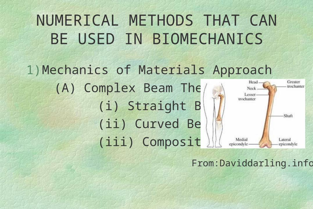
Energy method
Total potential energy must be stationary
δ (U + W) = δ ( П ) = 0

Introduction
Residual method
Differential equation governing the problem is given by A ( ø ) = 0
Minimise R = A ( ø* ) - A ( ø )
ø is actual solution
ø* is assumed solution

Introduction
Both methods give us a set of equations
[ K ] { a } = { f }
Stiffness Matrix
Displacement Matrix
Force Matrix

Introduction - FEM Procedure
Continuum is separated by imaginary lines or surfaces into a number of “finite elements”
Finite Elements

Introduction - FEM Procedure Elements are assumed to be interconnected at a
discrete number of “nodal points” situated on their boundaries
Finite ElementsNodal Points
Displacements at these nodal points will be the basic unknown

Introduction - FEM Procedure A set of functions is chosen to define uniquely the
state of displacement within each finite element ( U ) in terms of nodal displacements ( a1 , a2 , a3 )
U = Σ Ni ai i= 1, 3
x
y
a1
a2
a3
Finite Element
Nodal Point

Introduction - FEM Procedure This displacement function is input into either
“energy equations” or “residual equations” to give us element equilibrium equation
[ K ] { a } = { f }
x
y
a1
a2
a3
Finite Element
Nodal Point
ElementDisplacementMatrix
ElementForceMatrix
ElementStiffnessMatrix

Introduction - FEM ProcedureElement equilibrium equations are assembled
taking care of displacement compatibility at the connecting nodes to give a set of equations that represents equilibrium of the entire continuum
Finite ElementsNodal Points

Introduction - FEM ProcedureSolution for displacements are obtained after
substituting boundary conditions in the continuum equilibrium equations
Finite ElementsNodal Points
Support PointsSupport Points

Introduction Finite element method used to solve:
Elastic continuum Heat conduction Electric & Magnetic potential Non-linear (Material & Geometric) -plasticity, creep Vibration Transient problems Flow of fluids Combination of above problems Fracture mechanics

Introduction Finite elements:
Truss , Cable and Beam elements Two & Three solid elements Axi-symmetric elements Plate & Shell elements Spring, Damper & Mass elements Fluid elements
Application to Spine Biomechanics
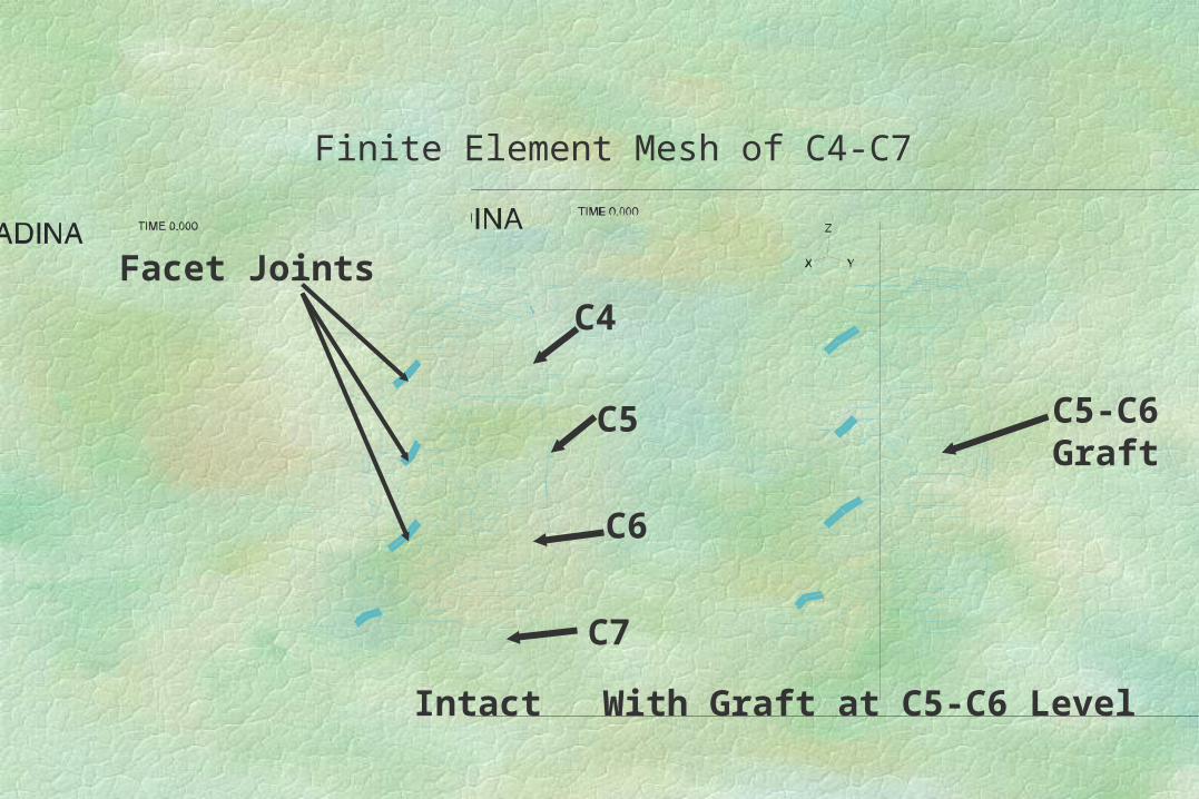
Finite Element Mesh of C4-C7
Intact With Graft at C5-C6 Level
C4
C5
C6
C7
C5-C6Graft
Facet Joints

von Mises Stress in C4-C5 Annulus (Flexion)
Neutral Graft Kyphotic Graft
5 MPa 6 MPaAnterior Anterior

Finite Element Mesh of L1-S1

Vertical Displacement Distribution in L1-S1

Finite Element Mesh of L2-L5With 25% Translational
Spondylolisthesis

Vertical Displacement Distribution in L2-L5 Under Flexion Moment
(25% translational spondylolisthesis)

Application to Knee Implant Biomechanics

Finite Element Mesh to Represent Tibial Insert & Femoral Component

Contact Compressive Stress

Motion of Femoral Implant with respect to UHMWPE Knee Insert

Application to Femoral Implant Biomechanics

Finite Element Mesh of an Intact Femur

Distribution of SIGMA-ZZ in an intact femur

Finite Element Mesh of a Femur with Implant

SIGMA-ZZ in a Femur With Implant

Implant fixed with cement layer in a femur

Von Misses stress in cement layer

SIGMA-ZZ in cortical bone in a femur with implant attached using cement

Advantage of using FEMIrregular complex geometry can be modeledEffect of large number of variables in a problem
can be easily analysedMultiple phase problems can be modeledEffect of various surgical techniques can be
compared using appropriate FE modelsBoth static and time dependent problems can be
modeledSolution to certain problems that cannot be (or
difficult) obtained otherwise can be solved by FEM