Embed Size (px)
Citation preview
Numerical Methods for the Multi-Physical Analysis of Long Span Cable-Stayed Bridges
DISSERTATION
zur Erlangung des akademischen Grades
Doktor-Ingenieur (Dr.-Ing.)
an der Fakultät Bauingenieurwesen
der
Bauhaus-Universität Weimar
vorgelegt von
M.Sc. Nazim Abdul Nariman
geboren am 15 Februar 1971 in Kirkuk - Irak
(Interner Doktorand)
Weimar, November 2, 2017
Mentor:
Prof. Dr.-Ing. Timon Rabczuk, Bauhaus-Universität Weimar
Gutachter:
Prof. Dr. Ir. Magd Abdel Wahab, Ghent University, Belgium
Prof. Dr. rer. nat. Tom Lahmer, Bauhaus-Universität Weimar


This work is dedicated to:
The souls of my beloved mother and father
&
To my loyal wife (Heero) and dearest sons (Revan) and (Avyar)

Acknowledgements
First of all, I thank my God who granted me the strength and the determination to complete
my doctorate study at Bauhaus Universität-Weimar in Germany.
I am deeply indebted to my dear supervisor Prof. Dr.-Ing.Timon Rabczuk, for his constant
support, valuable advice and guidance. Actually without his encouragement and
understanding of many obstacles encountered during my PhD study, it would have been
nearly impossible to continue and complete.
I would also like to give a special thanks to Prof. Dr.-Ing.Guido Morgenthal for providing a
wealth of helpful advice and guidance related to the area of wind effects on long span
bridges and validation process.
My grateful thanks are also to Prof. Dr. rer. nat. Tom Lahmer for his recommendations
regarding the field of sensitivity analysis.
I owe my most sincere gratitude to my wife Heero and sons Revan and Avyar for enduring
so much and remaining alone for a long time so that to support me.
Lastly, I would like to thank Dr.-Ing. Mohammed Msekh for assisting me in many directions
during my study in Weimar, I am grateful to him.
Nazim Abdul Nariman
Weimar, September 23, 2016

Ehrenwörtliche Erklärung
Ich erkläre hiermit ehrenwörtlich, dass ich die vorliegende Arbeit ohne unzulässige Hilfe
Dritter und ohne Benutzung anderer als der angegebenen Hilfsmittel angefertigt habe. Die
aus anderen Quellen direkt oder indirekt übernommenen Daten und Konzepte sind unter
Angaben der Quellen gekennzeichnet.
Weitere Personen waren an der inhaltlich-materiellen Erstellung der vorliegenden Arbeit
nicht beteiligt. Insbesondere habe ich hierfür nicht die entgeltliche Hilfe von Vermittlungs-
bzw. Beratungsdiensten (Promotionsberater oder anderer Personen) in Anspruch
genommen. Niemand hat von mir unmittelbar oder mittelbar geldwerte Leistungen für
Arbeiten erhalten, die im Zusammenhang mit dem Inhalt der vorgelegten Dissertation
stehen.
Die Arbeit wurde bisher weder im In-noch im Ausland in gleicher oder ähnlicher Form einer
anderen Prfungsbehörde vorgelegt.
Ich versichere ehrenwörtlich, dass ich nach bestem Wissen die reine Wahrheit gesagt und
nichts verschwiegen habe.
Nazim Abdul Nariman
Weimar, September 23, 2016
This dissertation has been constructed supporting on the following published papers:
1- Nariman N. A. (2017). Thermal Fluid-Structure Interaction and Coupled Thermal-Stress Analysis in a Cable Stayed Bridge Exposed to Fire. Frontiers of Structural and Civil Engineering, doi:10.1007/s11709-017-0452-4. 2- Nariman N. A. (2017). Kinetic Energy Based Model Assessment and Sensitivity Analysis of Vortex Induced Vibration of Segmental Bridge Decks. Frontiers of Structural and Civil Engineering, 11(4), 480-501. 3- Nariman N. A. (2017). Aerodynamic Stability Parameters Optimization and Global Sensitivity Analysis for a Cable Stayed Bridge. KSCE Journal of Civil Engineering, 21(5), 1866-1881. 4- Nariman N. A. (2017). Control Efficiency Optimization and Sobol's Sensitivity Indices of MTMDs Design Parameters for Buffeting and Flutter Vibrations in a Cable Stayed Bridge. Frontiers of Structural and Civil Engineering, 11(1), 66-89. 5- Nariman N. A. (2017). A Novel Structural Modification to Eliminate the Early Coupling between Bending and Torsional Mode Shapes in a Cable Stayed Bridge. Frontiers of Structural and Civil Engineering, 11(2), 131-142. 6- Nariman N. A. (2016). Influence of Fluid-Structure Interaction on Vortex Induced Vibration and Lock-in Phenomena in Long Span Bridges. Frontiers of Structural and Civil Engineering, 10(4), 363-384.


Abstract
The main categories of wind effects on long span bridge decks are buffeting, flutter, vortex-
induced vibrations (VIV) which are often critical for the safety and serviceability of the
structure. With the rapid increase of bridge spans, research on controlling wind-induced
vibrations of long span bridges has been a problem of great concern.The developments of
vibration control theories have led to the wide use of tuned mass dampers (TMDs) which has
been proven to be effective for suppressing these vibrations both analytically and
experimentally. Fire incidents are also of special interest in the stability and safety of long
span bridges due to significant role of the complex phenomenon through triple interaction
between the deck with the incoming wind flow and the thermal boundary of the surrounding
air.
This work begins with analyzing the buffeting response and flutter instability of three
dimensional computational structural dynamics (CSD) models of a cable stayed bridge due to
strong wind excitations using ABAQUS finite element commercial software. Optimization
and global sensitivity analysis are utilized to target the vertical and torsional vibrations of the
segmental deck through considering three aerodynamic parameters (wind attack angle, deck
streamlined length and viscous damping of the stay cables). The numerical simulations results
in conjunction with the frequency analysis results emphasized the existence of these
vibrations and further theoretical studies are possible with a high level of accuracy. Model
validation is performed by comparing the results of lift and moment coefficients between the
created CSD models and two benchmarks from the literature (flat plate theory) and flat plate
by (Xavier and co-authors) which resulted in very good agreements between them. Optimum
values of the parameters have been identified. Global sensitivity analysis based on Monte
Carlo sampling method was utilized to formulate the surrogate models and calculate the
sensitivity indices. The rational effect and the role of each parameter on the aerodynamic
stability of the structure were calculated and efficient insight has been constructed for the
stability of the long span bridge.
2D computational fluid dynamics (CFD) models of the decks are created with the support of
MATLAB codes to simulate and analyze the vortex shedding and VIV of the deck. Three
aerodynamic parameters (wind speed, deck streamlined length and dynamic viscosity of the
air) are dedicated to study their effects on the kinetic energy of the system and the vortices
shapes and patterns. Two benchmarks from the literature (Von Karman) and (Dyrbye and
Hansen) are used to validate the numerical simulations of the vortex shedding for the CFD
models. A good consent between the results was detected. Latin hypercube experimental

method is dedicated to generate the surrogate models for the kinetic energy of the system and
the generated lift forces. Variance based sensitivity analysis is utilized to calculate the main
sensitivity indices and the interaction orders for each parameter. The kinetic energy approach
performed very well in revealing the rational effect and the role of each parameter in the
generation of vortex shedding and predicting the early VIV and the critical wind speed.
Both one-way fluid-structure interaction (one-way FSI) simulations and two-way fluid-
structure interaction (two-way FSI) co-simulations for the 2D models of the deck are executed
to calculate the shedding frequencies for the associated wind speeds in the lock-in region in
addition to the lift and drag coefficients. Validation is executed with the results of (Simiu and
Scanlan) and the results of flat plate theory compiled by (Munson and co-authors)
respectively. High levels of agreements between all the results were detected. A decrease in
the critical wind speed and the shedding frequencies considering (two-way FSI) was
identified compared to those obtained in the (one-way FSI). The results from the (two-way
FSI) approach predicted appreciable decrease in the lift and drag forces as well as prediction
of earlier VIV for lower critical wind speeds and lock-in regions which exist at lower natural
frequencies of the system. These conclusions help the designers to efficiently plan and
consider for the design and safety of the long span bridge before and after construction.
Multiple tuned mass dampers (MTMDs) system has been applied in the three dimensional
CSD models of the cable stayed bridge to analyze their control efficiency in suppressing both
wind -induced vertical and torsional vibrations of the deck by optimizing three design
parameters (mass ratio, frequency ratio and damping ratio) for the (TMDs) supporting on
actual field data and minimax optimization technique in addition to MATLAB codes and Fast
Fourier Transform technique. The optimum values of each parameter were identified and
validated with two benchmarks from the literature, first with (Wang and co-authors) and then
with (Lin and co-authors). The validation procedure detected a good agreement between the
results. Box-Behnken experimental method is dedicated to formulate the surrogate models to
represent the control efficiency of the vertical and torsional vibrations. Sobol's sensitivity
indices are calculated for the design parameters in addition to their interaction orders. The
optimization results revealed better performance of the MTMDs in controlling both the
vertical and the torsional vibrations for higher mode shapes. Furthermore, the calculated
rational effect of each design parameter facilitates to increase the control efficiency of the
MTMDs in conjunction with the support of the surrogate models which simplifies the process
of analysis for vibration control to a great extent.
A novel structural modification approach has been adopted to eliminate the early coupling
between the bending and torsional mode shapes of the cable stayed bridge. Two lateral steel

beams are added to the middle span of the structure. Frequency analysis is dedicated to obtain
the natural frequencies of the first eight mode shapes of vibrations before and after the
structural modification. Numerical simulations of wind excitations are conducted for the 3D
model of the cable stayed bridge. Both vertical and torsional displacements are calculated at
the mid span of the deck to analyze the bending and the torsional stiffness of the system
before and after the structural modification. The results of the frequency analysis after
applying lateral steel beams declared that the coupling between the vertical and torsional
mode shapes of vibrations has been removed to larger natural frequencies magnitudes and
higher rare critical wind speeds with a high factor of safety.
Finally, thermal fluid-structure interaction (TFSI) and coupled thermal-stress analysis are
utilized to identify the effects of transient and steady state heat-transfer on the VIV and
fatigue of the deck due to fire incidents. Numerical simulations of TFSI models of the deck
are dedicated to calculate the lift and drag forces in addition to determining the lock-in
regions once using FSI models and another using TFSI models. Vorticity and thermal fields
of three fire scenarios are simulated and analyzed. The benchmark of (Simiu and Scanlan) is
used to validate the TFSI models, where a good agreement was manifested between the two
results. Extended finite element method (XFEM) is adopted to create 3D models of the cable
stayed bridge to simulate the fatigue of the deck considering three fire scenarios. The
benchmark of (Choi and Shin) is used to validate the damaged models of the deck in which a
good coincide was seen between them. The results revealed that the TFSI models and the
coupled thermal-stress models are significant in detecting earlier vortex induced vibration and
lock-in regions in addition to predicting damages and fatigue of the deck and identifying the
role of wind-induced vibrations in speeding up the damage generation and the collapse of the
structure in critical situations.


xii
Contents
Contents…………………………………………………………………………………………….xii
List of Figures…………………………………………………………………………………..xviii
List of Tables…………………………………………………………………………………….xxiv
Nomenclature………………………………………………………………………………….....xxv
1 Introduction……………………………………………………………………………………..1
1.1 Background…………………………………………………………………………….......1
1.2 State of The Art………………………………………………………………………….....5
1.3 Literature Review………………………………………………………………………......6
1.4 Aim and Objectives of Work…………………………………………………………….....8
1.5 Methodology………………………………………………..................................................9
1.6 Dissertation Outline ………………………………………………………………………..12
2 Aerodynamic Stability of Long Span Bridges……………………………………........16
2.1 Vertical and Torsional Vibrations ………………………………………………………...16
2.2 Aerodynamic Stability Parameters………………………………………………………...17
2.2.1 Wind Attack Angle………………………………………………………………..17
2.2.2 Deck Section……………………………………………………………………...18
2.2.3 Viscous Damping of Stay Cables………………………………………………....18
2.3 Equation of Motion………………………………………………………………………..19
2.3.1 Aerodynamic Forces and Moment……………………………………………….20
2.4 Finite Element Model……………………………………………………………………...21
2.4.1 Mesh Convergence……………………………………………………………….22
2.4.2 Wind Load………………………………………………………………………..23
2.4.3 Frequency Analysis………………………………………………………………24
2.4.4 Results of Mode Shapes………………………………………………………….24
2.4.5 Simulation of The Mode Shapes…………………………………………………25
2.5 Aerodynamic Instability Analysis…………………………………………………………26
2.5.1 Results of Vertical Vibrations……………………………………………………26
2.5.2 Results of Torsional Vibrations…………………………………………………..27

xiii
2.5.3 Simulation of Aerodynamic Instability….……………………………………….27
2.6 Aerodynamic Parameters Optimization …………………………………………………..29
2.6.1 Results of Wind Attack Angle Effect …………………………………………...30
2.6.2 Results of Deck Streamlined Length Effect …………………………………….31
2.6.3 Results of Stay Cables Viscous Damping Effect………………………………...32
2.7 Validation of The FE Models………………………………………………………….….33
2.7.1 Flat Plate Theory Benchmark …………………………………………………...33
2.7.2 Flat Plate Model (Xavier and Co-authors) Benchmark ………………………....34
2.8 Sensitivity Analysis………………………………………………………………………35
2.9 Experimental Design……………………………………………………………………..35
2.9.1 Monte Carlo Sampling………………………………………………………….36
2.9.2 Probability Distribution………………………………………………………....36
2.9.3 Response Surface Methodology………………………………………………...37
2.9.4 Sobol’s Sensitivity Indices……………………………………………………...38
2.9.5 Results and Discussion of The Surrogate Models……………………………....39
2.9.6 Results and Discussion of The Sensitivity Indices……………………………...43
2.9.7 Convergence of The Results…………………………………………………….44
3 Kinetic Energy Based Model Assessment……………………………………………...47
3.1 Von Karman Vortex Street ………………………………………………………….........47
3.2 VIV Parameters…………………………………………………………………………...48
3.2.1 Reynolds Number……………………………………………………………….48
3.2.2 Deck Shape……………………………………………………………………...49
3.2.3 Dynamic Viscosity of Air……………………………………………………….49
3.3 Vortex Shedding Phenomenon in Bridges……………………………………………….50
3.4 Finite Element Model…………………………………………………………………….51
3.4.1 Mesh Convergence……………………………………………………………...53
3.5 Results of Vorticity and Kinetic Energy………………………………………………….55
3.5.1 Wind Speed Effect……………………………………………………………....55
3.5.2 Deck Streamlined Length Effect………………………………………………..58
3.5.3 Dynamic Viscosity of Air Effect………………………………………………..60
3.6 Validation of 2D-CFD Models…………………………………………………….……..62
3.6.1 Von Karman Benchmark………………………………………………………..62

xiv
3.6.2 Dyrbye and Hansen Benchmark……………………………………………….63
3.7 Sensitivity Analysis……………………………………………………………………...64
3.7.1 Latin Hypercube Sampling…………………………………………………….64
3.8 Surrogate Model Results and Discussion……………………………………………….65
3.9 Sensitivity Analysis Results and Discussion……………………………………………69
3.9.1 Convergence of The Results…………………………………………………...69
4 Fluid-Structure Interaction and Lock-In Phenomenon…………………………..73
4.1 Vortex Induced Vibration (VIV)………………………………………………………..73
4.2 Fluid-Structure Interaction (FSI)………………………………………………………..74
4.2.1 One-Way FSI…………………………………………………………………..74
4.2.2 Two-Way FSI……………………….…………………………………………75
4.3 Finite Element Models………………………………………………………………......76
4.3.1 Boundary Conditions ………………………………………………………….78
4.4 Results and Discussion………………………………………………………………….79
4.4.1 Vortex Shedding Simulation…………………………………………………...79
4.4.2 Lift Forces……………………………………………………………………...81
4.4.3 Drag Forces…………………………………………………………………….83
4.4.4 Kinetic Energy…………………………………………………………………86
4.4.5 Lock-In Phenomenon…………………………………………………………..86
4.4.6 Lift Coefficient…………………………………………………………………88
4.4.7 Drag Coefficient………………………………………………………………..89
4.4.8 Reynolds Number……………………………………………………………...90
4.4.9 Strouhal Number………………………………………………………………90
4.5 Validation of The FSI Models…………………………………………………………..92
4.5.1 Simiu and Scnlan Benchmark…………………………………………………..92
4.5.2 Flat Plate Model (Munson and Co-authors) Benchmark ……………………...93
5 Control Efficiency Optimization of Multiple Tuned Mass Dampers…………95
5.1 Tuned Mass Damper (TMD)……………………………………………………………95
5.1.1 Energy Dissipation Mechanism………………………………………………...96
5.2 Multiple Tuned Mass Dampers (MTMDs)……………………………………………..96
5.3 Concept of TMD Using Two-Mass System…………………………………………….97
5.4 Equation of Motion……………………………………………………………………..99

xv
5.5 Finite Element Model of The TMD…………………………………………………….102
5.5.1 Mode Shapes Analysis………………………………………………………...103
5.6 Optimization of TMD Parameters……………………………………............................106
5.6.1 Optimum Mass Ratio………………………………………………………….106
5.6.2 Results and Discussion……………………………………………………..…107
5.6.3 Simulation of The Models…………………………………………………….109
5.6.4 Optimum Frequency Ratio……………………………………………………109
5.6.5 Results and Discussion………………………………………………………..110
5.6.6 Optimum Damping Ratio……………………………………………………..112
5.6.7 Results and Discussion………………………………………………………..113
5.7 Validation of The TMDs Models………………………………………………………114
5.7.1 Wang and Co-authors Benchmark…………………………………………….115
5.7.2 Lin and Co-authors Benchmark……………………………………………...116
5.8 Global Sensitivity Analysis…………………………………………………………….116
5.9 Box-Behnken Sampling Method……………………………………………………….117
5.9.1 Surrogate Models Results…………………………………………………….119
5.9.2 Sensitivity Indices Results and Discussion…………………………………..120
5.9.3 Convergence of The Results………………………………………………….122
6 Novel Structural Modification………………………………………………………….125
6.1 Flutter Wind Speed……………………………………………………………………..125
6.2 Flutter Analysis………………………………………………………………………....125
6.3 Finite Element Model After Modification……………………………………………...127
6.3.1 Structural Modification and Mode Shapes……………………………………129
6.3.2 Results of Vertical Displacements…………………………………………….132
6.3.3 Results of Torsional Displacements…………………………………………...132
6.4 Results of Control Efficiency…………………………………………………………...133
7 Thermal Fluid-Structure Interaction and Coupled Thermal-Stress Analysis
Due to Fire…………………………………………………………………………………...135
7.1 Standard Temperature-Time Fire Curve ……………………………………………….135
7.2 Heat-Transfer Analysis ………………………………………………………………...136
7.2.1 Thermal Analysis of a Cable Stayed Bridge …………………………………..137
7.2.2 Heat-Transfer Theory ……………….................................................................137

xvi
7.2.3 Thermal Boundary Conditions ………………………………………………..138
7.3 Thermal Fluid-Structure Interaction …………………………………………………...138
7.3.1 Governing Equations …………………………………………………………139
7.3.2 Fluid Model .………………………………………………………………….139
7.3.3 Solid Model …………………………………………………………………..140
7.4 Finite Element Model of TFSI…………………………………………………………140
7.4.1 Fire Scenarios…………………………………………………………………142
7.4.2 Results of TFSI-Models Simulations……………………………………….....143
7.4.3 Results of Lift and Drag Forces-FSI-Models…………………………………144
7.4.4 Results of Lift and Drag Forces-TFSI-Models……………………………….146
7.4.5 Results of Lock-in Phenomenon ……………………………………………...148
7.5 Validation of TFSI-Models…………………………………………………………….150
7.6 Coupled Thermal-Stress Analysis………………………………………………………150
7.6.1 Thermal Cracking and Spalling of Concrete ………………………………....151
7.6.2 Finite Element Model of Coupled Thermal-Stress ………………………….152
7.6.3 Results of Deck Displacements ……………………………………...............153
7.6.4 Extended Finite Element Method ………...………………………………….155
7.6.5 Results of Cracking and Spalling of The Deck………………………………157
7.7 Validation of Coupled Thermal - Stress Models………………………………………160
8 Conclusions and Recommendations for Further Research………………........162
8.1 Conclusions.……………………………………………………………………………162
8.2 Recommendations for Further Researches …………………………………………….166
Appendix A…………………………………………………………………………………..168 A.1 Mesh Convergence……………………………………………………………………...168
A.2 Surrogate Models Equations for Vertical and Torsional Responses (MATLAB Codes)…………………………………………………………………………………………………168
A.3 Lift Force and Aerodynamic Parameters……………………………………………….169
A.4 Surrogate Models Equations for Kinetig Energy and Lift Force (MATLAB Codes)….170
A.5 Effect of TMD’s Design Parameters on Vertical and Torsional Responses…………....170
A.6 Surrogate Models Equations for Vertical and Torsional Control Efficiencies (MATLAB Codes)…………………………………………………………... ……………………………………172
References……………………………………………………………………………………..173

xvii

xviii
List of Figures 2.1 Vertical and torsional motions of the deck……………………………………………………16
2.2 Aerodynamic characterization of a section……………………………………………………18
2.3 Sag of a stay cable and viscous damping……………………………………………………...19
2.4 Mesh convergence considering four mode shapes of vibrations……………………………...22
2.5 Wind speed fluctuation time history…………………………………………………………..23
2.6 Wind pressure and the FE model……………………………………………………………...23
2.7 Eight mode shapes of vibrations (Frequency Analysis)……………………………………….25
2.8 Time history of vertical vibration at mid-span center of the deck…………………………….26
2.9 Time history of flutter vibration at mid-span edges of the deck………………………………27
2.10 Eight simulations of vibration in the cable stayed bridge model……………………………..28
2.11 Wind attack angle effect on the vertical displacement of the deck …………………………..30
2.12 Wind attack angle effect on the torsional displacement of the deck………………………….30
2.13 Deck streamlined length effect on the vertical displacement of the deck…………………….31
2.14 Deck streamlined length effect on the torsional displacement of the deck…………………...31
2.15 Viscous damping of stay cables effect on the vertical displacement of the deck…………….32
2.16 Viscous damping of stay cables effect on the torsional displacement of the deck…………...33
2.17 Lift coefficient with wind attack angle validation……………………………………….34
2.18 Moment coefficient with wind attack angle validation…………………………………34
2.19 Coefficient of determination between actual and predicted vertical displacement……………....40
2.20 Response surface plot showing effect of X1 and X2 on the predicted vertical displacement…………………………………………………………………………………………….40
2.21 Response surface plot showing effect of X1 and X3 on the predicted vertical displacement…………………………………………………………………………………………….41
2.22 Response surface plot showing effect of X2 and X3 on the predicted vertical displacement…………………………………………………………………………………………….41
2.23 Coefficient of determination between actual and predicted torsional displacement…………….41
2.24 Response surface plot showing effect of X1 and X2 on the predicted torsional displacement…………………………………………………………………………………………….42
2.25 Response surface plot showing effect of X1 and X3 on the predicted torsional displacement…………………………………………………………………………………………….42
2.26 Response surface plot showing effect of X2 and X3 on the predicted torsional displacement…………………………………………………………………………………………….42

xix
2.27 Convergence of sensitivity indices-Vertical displacement…………………………………...44
2.28 Convergence of sensitivity indices-Torsional displacement………………………………….45
3.1 Karman-Bernard’s (Von Karman) vortex street……………………………………………...47
3.2 Vortex Street for a bluff body (Dyrbye and Hansen, 1999)………………………………….48
3.3 Dynamic viscosity of air versus temperature…………………………………………………50
3.4 Schematic flow around a stationary bridge deck……………………………………………..51
3.5 Deck model dimensions………………………………………………………………………52
3.6 Flow domain size in CFD…………………………………………………………………….52
3.7 Vortex shedding-Mesh size 28074 elements………………………………………………….53
3.8 Vortex shedding-Mesh size 9943 elements…………………………………………………...53
3.9 Vortex shedding- Mesh size 7724 elements…………………………………………………..54
3.10 Vortex shedding-Mesh size 6202 elements…………………………………………………...54
3.11 Vortex shedding-Mesh size 5317 elements…………………………………………………...54
3.12 Vortex shedding-Velocity field-V=0.5 m/s…………………………………………………...55
3.13 Vortex shedding-Vorticity field-V=0.5 m/s…………………………………………………...55
3.14 Vortex shedding-Velocity field-V=12.5 m/s………………………………………………….56
3.15 Vortex shedding-Vorticity field-V=12.5 m/s …………………………………………………56
3.16 Vortex shedding-Velocity field-V=25 m/s……………………………………………………56
3.17 Vortex shedding-Vorticity field-V=25 m/s…………………………………………………...56
3.18 Wind speed V = 0.5 m/s and the kinetic energy of the system………………………………..57
3.19 Wind speed V = 12.5 m/s and the kinetic energy of the system………………………………57
3.20 Wind speed V = 25 m/s and the kinetic energy of the system………………………………...58
3.21 Effect of wind speed on the kinetic energy of the system…………………………………….58
3.22 Vortex shedding-Velocity field-Deck streamlined length L = 0 m…………………………...59
3.23 Vortex shedding-Velocity field-Deck streamlined length L = 1 m…………………………...59
3.24 Vortex shedding-Velocity field-Deck streamlined length L = 2 m…………………………...59
3.25 Effect of deck streamlined length on the kinetic energy of the system……………………….60
3.26 Vortex shedding-Velocity field-Air dynamic viscosity μ=1.632E-5………………………….61
3.27 Vortex shedding-Velocity field-Air dynamic viscosity μ=1.757E-5………………………….61
3.28 Vortex shedding-Velocity field-Air dynamic viscosity μ =1.882E-5…………………………61
3.29 Effect of air dynamic viscosity on the kinetic energy of the system………………………….62

xx
3.30 Wind speed and ratio of two vortices rows central distance to one row vortices central distance validation……………………………………………………………………………………………….63
3.31 Wind speed and one row vortices central distance validation………………………………...64
3.32 Coefficient of determination between actual and predicted kinetic energy………………………66
3.33 Response surface plot showing effect of X1 and X2 on the predicted kinetic energy………..66
3.34 Response surface plot showing effect of X1 and X3 on the predicted kinetic energy………..66
3.35 Response surface plot showing effect of X2 and X3 on the predicted kinetic energy………..67
3.36 Coefficient of determination between actual and predicted lift force…………………………….67
3.37 Response surface plot showing effect of X1 and X2 on the predicted lift force……………...68
3.38 Response surface plot showing effect of X1 and X3 on the predicted lift force……………...68
3.39 Response surface plot showing effect of X2 and X3 on the predicted lift force……………...68
3.40 Convergence of sensitivity indices-Kinetic energy…………………………………………...70
3.41 Convergence of sensitivity indices-Lift force………………………………………………....71
4.1.a Deck model dimensions………………………………………………………………………77
4.1.b Flow domain size……………………………………………………………………………..77
4.1.c The CSD model ……………………………………………………………………………...77
4.2 Domains and fluid–structure interaction boundary conditions……………………………….78
4.3.a CFD mesh size-9943 elements………………………………………………………………..79
4.3.b CSD mesh size-357 elements…………………………………………………………………79
4.4 Vortex shedding one-way V=1 m/s…………………………………………………………...80
4.5 Vortex shedding two-way V=1 m/s…………………………………………………………...80
4.6 Vortex shedding one-way V=10 m/s………………………………………………………….80
4.7 Vortex shedding two-way V=10 m/s………………………………………………………….80
4.8 Vortex shedding one-way V=15 m/s………………………………………………………….81
4.9 Vortex shedding two-way V=15 m/s………………………………………………………….81
4.10 Time history of lift forces V=1 m/s…………………………………………………………...81
4.11 Time history of lift forces V=5 m/s…………………………………………………………...82
4.12 Time history of lift forces V=10 m/s………………………………………………………….82
4.13 Time history of lift forces V=15 m/s………………………………………………………….83
4.14 Time history of drag forces V=1 m/s………………………………………………………….84
4.15 Time history of drag forces V=5 m/s………………………………………………………….84

xxi
4.16 Time history of drag forces V=10 m/s………………………………………………………..85
4.17 Time history of drag forces V=15 m/s………………………………………………………..85
4.18 Time history of the simulations kinetic energy……………………………………………….86
4.19 Vortex shedding at Lock-in region……………………………………………………………87
4.20 Wind speed versus Vortex shedding frequency - Lock-In phenomenon……………………..88
4.21 Reynolds number versus lift coefficient………………………………………………………89
4.22 Reynolds number versus drag coefficient……………………………………………………..89
4.23 Reynolds number versus Strouhal number……………………………………………………91
4.24 Wind speed versus Vortex shedding frequency- Lock-in phenomenon validation……….…..92
4.25 Reynolds number versus drag coefficient validation………………………………………….93
5.1 TMD attached to the primary mass…………………………………………………………...98
5.2 Location of TMDs for suppressing a- Vertical vibration and b- Torsional vibration ………100
5.3 Positioning the TMDs……………………………………………………………………......102
5.4 Wind speed fluctuation profile……………………………………………………………….103
5.5 Eight mode shapes of vibrations……………………………………………………………..104
5.6 Power spectral densities of vertical and torsional displacements at the mid span…………...105
5.7 TMD mass ratio effect on the vertical vibration……………………………………………..107
5.8 TMD mass ratio effect on torsional vibration………………………………………………..108
5.9 TMDs mass ratio effect on vertical and torsional vibrations………………………………...109
5.10 TMD frequency ratio effect on the vertical vibration………………………………………..111
5.11 TMD frequency ratio effect on torsional vibration…………………………………………..112
5.12 TMD damping ratio effect on the vertical vibration…………………………………………113
5.13 TMD damping ratio effect on the torsional vibration………………………………………..114
5.14 Validation for TMDs mass ratio effect on the vertical vibration of the deck………………..115
5.15 Validation for TMDs damping ratio effect on the vertical vibration of the deck…………....116
5.16 Box-Behnken experimental design………………………………………………………….117
5.17 Coefficient of determination-Vertical vibration control efficiency……………………………...120
5.18 Coefficient of determination-Torsional vibration control efficiency……………………………120
5.19 Convergence of sensitivity indices-Vertical vibration control efficiency…………………...122
5.20 Convergence of sensitivity indices-Torsional vibration control efficiency…………………123

xxii
6.1 Wind induced forces (lift and drag) and moment in the deck……………………………….126
6.2 Finite element model before structural modification………………………………………...128
6.3 Finite element model after structural modification…………………………………………..128
6.4 Wind speed fluctuation time history………………………………………………………...128
6.5 Sixteen mode shapes of vibrations before and after structural modification………………...131
6.6 Time history of vertical vibrations at center of the deck mid-span………………………….132
6.7 Time history of torsional vibrations at outer edges of the deck mid-span…………………...133
7.1 ISO 834 Standard temp - Time fire curve…………………………………………………...135
7.2 The heat- transfer process of a segmental bridge deck exposed to fire……………………...137
7.3 Deck TFSI-model dimensions……………………………………………………………….141
7.4.a Segmental deck exposed to fire scenarios-Fire scenario 1………………………………….142
7.4.b Segmental deck exposed to fire scenarios-Fire scenario 2………………………………….142
7.4.c Segmental deck exposed to fire scenarios-Fire scenario 3………………………………….142
7.5.a TFSI-Models-Fire scenarios-Fire scenario 1-Vorticity field ……………………………….144
7.5.b TFSI-Models-Fire scenarios- Fire scenario 1-Temperature field.…………………………..144
7.5.c TFSI-Models-Fire scenarios-Fire scenario 2-Vorticity field………………………………..144
7.5.d TFSI-Models-Fire scenarios-Fire scenario 2-Temperature field…………………………....144
7.5.e TFSI-Models-Fire scenarios-Fire scenario 3-Vorticity field………………………………..144
7.5.f TFSI-Models-Fire scenarios-Fire scenario 3-Temperature field…………………………….144
7.6.a Lift and drag forces-FSI models- No Fire…………………………………………………...145
7.6.b Lift and drag forces-FSI models-Fire scenario1…………………………………………….145
7.6.c Lift and drag forces-FSI models-Fire scenario 2……………………………………………145
7.6.d Lift and drag forces-FSI models-Fire scenario 3……………………………………………145
7.7.a Lift and drag forces-TFSI models-No Fire………………………………………………….147
7.7.b Lift and drag forces-TFSI models-Fire scenario1…………………………………………...147
7.7.c Lift and drag forces-TFSI models-Fire scenario 2…………………………………………..147
7.7.d Lift and drag forces-TFSI models-Fire scenario 3…………………………………………..147
7.8 Lock-in Phenomenon - TFSI and FSI models ……………………………………………...149
7.9 Lock-in TFSI-models validation ……………………………………………………………150
7.10 Finite element 3D model of the cable stayed bridge………………………………………...152

xxiii
7.11 Horizontal displacement …………………………………………………………………....154
7.12 Vertical displacement………………………………………………………………………..154
7.13 Angular displacement ………………………………………………………………………154
7.14 Enriching shape functions of node 2 and node 3……………………………….……….......156
7.15 Crack in 3D by two level set functions ………………………………………....156
7.16 Maximum principal stress - Fire scenario 1- Without XFEM damage simulation ………....157
7.17 Maximum principal stress - Fire scenario 1- With XFEM damage simulation……………..157
7.18 Maximum principal stress - Fire scenario 2- Without XFEM damage simulation ………....158
7.19 Maximum principal stress - Fire scenario 2- With XFEM damage simulation …………….158
7.20 Maximum principal stress - Fire scenario 3- Without XFEM damage simulation ………....159
7.21 Maximum principal stress - Fire scenario 3- With XFEM damage simulation …………….159
A.1 Mesh convergence for mode shapes of vibrations………………………………………….168
A.3.1 Effect of wind speed on the generated lift force in the deck………………………………..169
A.3.2 Effect of deck streamlined length on the generated lift force in the deck…………………..169
A.3.3 Effect of air dynamic viscosity on the generated lift force in the deck……………………..169
A.5.1 Effect of TMD mass ratio on the vertical vibration of the deck…………………………….170
A.5.2 Effect of TMD mass ratio on the torsional vibration of the deck…………………………...170
A.5.3 Effect of TMD frequency ratio on the vertical vibration of the deck……………………….171
A.5.4 Effect of TMD frequency ratio on the torsional vibration of the deck……………………...171
A.5.5 Effect of TMD damping ratio on the vertical vibration of the deck………………………...171
A.5.6 Effect of TMD damping ratio on the torsional vibration of the deck……………………….172

xxiv
List of Tables 2.1 Material properties …………………………………………………………………………....22
2.2 Modes and frequencies……………………………………………………………………......24
2.3 Aerodynamic parameters and range values…………………………………………………...29
2.4 Results of lift and moment coefficients for ABAQUS FE model and two benchmarks……...33
2.5 Range values and probability distributions for the aerodynamic parameters………………....36
2.6 Sensitivity indices of the aerodynamic parameters…………………………………………....43
3.1 Validation with Von Karman benchmark……………………………………………………..63
3.2 Validation with Dyrbye and Hansen benchmark……………………………………………...64
3.3 Sensitivity indices……………………………………………………………………………..70
4.1 Reynolds number versus lift and drag coefficients for multiple wind velocities……………..90
4.2 Strouhal number versus vortex shedding frequency for multiple wind velocities………….....91
5.1 Vibration modes data……………………………………………………………………..….103
5.2 Parameters of TMDs for multiple mass ratios……………………………………………….106
5.3 Vertical vibration control efficiency-Mass ratio …………………………………………….107
5.4 Torsional vibration control efficiency-Mass ratio …………………………………………..108
5.5 Parameters of the TMD for multiple frequency ratios ……………………………………....110
5.6 Vertical vibration control efficiency-Frequency ratio……………………………………….111
5.7 Torsional vibration control efficiency-Frequency ratio……………………………………...112
5.8 Parameters of the TMD for multiple damping ratios ………………………………………..112
5.9 Vertical vibration control efficiency-Damping ratio………………………………………...113
5.10 Torsional vibration control efficiency-Damping ratio ……………………………………....114
5.11 The level of variables chosen for the Box-Behnken design……………………………….....118
5.12 Box-Behnken design with coded and actual values for three size fractions ………………...119
5.13 Sensitivity indices……………………………………………………………………………121
6.1 Mode shapes and frequencies………………………………………………………………..129
7.1 Lock-in data for TFSI and FSI models ……………………………………………………...149
7.2 Mode shapes and frequencies………………………………………………………………..153

xxv
Nomenclature Abberviations FE Finite Element
VIV Vortex Induced Vibration
B.C Boundary Condition
CSD Computational Structural Dynamics
CFD Computational Fluid Dynamics
FSI Fluid-Structure Interaction
TMDs Tuned Mass Dampers
MTMDs Multiple Tuned Mass Dampers
FFT Fast Fourier Transform
PSD Power Spectral Density
TFSI Thermal Fluid-Structure Interaction
XFEM Extended Finite Element Method
Aerodynamic Stability Parameters
( )
( )
( )

xxvi
( )
( )
Kinetic Energy Based Model Assessment
( )
( )
xxvii
( )
( )
( )
Fluid-Structure Interaction and Lock-in Phenomenon
( )
Control Efficiency Optimization of MTMDs
xxviii

xxix
Novel Structural Modification
( )
Thermal Fluid-Structure Interaction and Coupled Thermal-Stress Analysis Due to Fire

xxx
Velocity of the fluid
( )
( )
( )
( )
( ) ( ( ))

xxxi

1
Chapter 1 Introduction 1.1 Background Long span bridges are vulnerable to many types of vibrations when subjected to wind
buffeting action due to their slenderness, high flexibility, low structural damping and
lightweight. Therefore their safety and serviceability are often critical due to wind-induced
vibrations. Buffeting action is a type of vibration motion induced by turbulent wind. The
natural wind is not steady but has a turbulent characteristic, so the wind fluctuations in the
vertical and horizontal directions are random in space, and thus the wind pressures along the
bridges are random in time and space. The coupled mode of vibrations which is resulting
from the deck-stay cables interaction at lower modes of vibrations is dominant and critical
case.The buffeting responses of the long span bridges increase and become more notable
when increasing the bridge span and the deck width. The internal forces and the
displacements resulted from buffeting responses are growing more apparent when the wind
speed is high. As a result many serious effects are arising such as fatigue of the structural
components and in critical cases result in the failure of the structure. The Tacoma incident is
the best example case of a wind induced failure. However significant numbers of bridges have
experienced extreme responses which were of sufficiently large amplitudes to be considered
at serious condition. Aerodynamic effect is the most important aspect of this type of vibration
and the greatest aerodynamic effect is caused by flutter. The flutter stability of bridge
structures is due to the critical wind speed. When flutter occurs, the wind forces change
continuously due to structural displacements, while the wind alters the stiffness and structural
damping of the system. When the free span of a bridge increases, the aerodynamic instability
increases. The critical wind speed would step down due to the resulting reduced torsional
stiffness particularly and the reduced bending stiffness. When the structural damping becomes
very low, a small oscillation would be amplified until the structural failure [Simiu and
Scanlan, 1996; Diana et al., 1998; Lin et al., 2000; Chen et al., 2001; Chen and Cai, 2003;
Chen et al., 2004; Valdebenito and Aparicio, 2006; Al-Assaf, 2006; Ubertini, 2008; Starossek
and Aslan, 2008; Janjic, 2010; Kwon, 2010; Patil, 2010; Van Vu. et al., 2011; Keerthana et
al., 2011; Kvamstad, 2011; Odden and Skyvulstad, 2012; Huang et al., 2012; Qin et al., 2013;
Mohammadi, 2013; Flamand et al., 2014; Xu, 2013; Xie et al., 2014; Xu et al., 2014].
When the aeroelastic interaction between the wind and the long span bridges is generated, the
flutter and the torsional instabilities can take place at certain wind speeds. The vibrational

1.1 Background
2
response of long span bridges is affected by many structural characteristics like mass,
stiffness and energy dissipation mechanisms [Ding and Lee, 2000; Man, 2004; He et al.,
2008; Ge and Xiang, 2008; Vairo, 2010; Zhang Xi, 2012; Shin et al., 2014]. Recently many
slender long span bridges have been constructed without taking in consideration the both the
bending and torsional stiffness, which resulted in wide displacements especially at the mid
span of the deck with probabilities of aeroelastic instability and structural failure. The extra
sensitivity of long span cable supported bridges due to wind excitation is related to the very
low structural damping in the coupled modes of vibrations widely below 1% and even less
than this value in the vibration modes associated with cable vibrations. Flutter and torsional
instabilities force limits on the length increase of long span cable supported bridges which can
be avoided by better aerodynamic design of the deck or by the use of vibration control
methods [Jones and Spartz, 1990; Pacheco et al., 1993; Cheng, 1999; Su et al., 2003; Fujino
et al., 2010; Wang et al., 2013; Phan and Nguyen, 2013; Xiong et al., 2014; Preumont et al.,
2015; Kusano, 2015; Haque, 2015; Bakis et al., 2016].
Vortex induced vibration (VIV) which is one of the wind-induced vibrations, is
predominantly decisive for the security and serviceability of these structures. The segmental
bridge decks are being selected supporting on many factors like structural and economic
characteristics, where the essential shape of the deck is not requisite to be aerodynamically
efficient optimally. Due to this fact, long span bridges are overwhelmingly undergo VIV
[Frandsen, 2004; Sarwar and Ishihara, 2010; Wu and Kareem, 2012; Fujino and Siringoringo,
2013]. Several research studies on the geometries and the vortex shedding mechanisms from
bluff bodies have been conducted. Presently the deck cross sections are designed between
bluff bodies and streamlined, for example the Tsing Lung Bridge in Hong Kong. The wind
flow in the wake region of a bluff body such as segmental bridge decks is described by
vortices which are shed from its trailing edge continuously at a particular frequency, where
they are often attributed to Karman vortices. The shape and the pattern of the vortices are
occasionally referred to Karman Street [Kiviluoma, 2001; Nicoli, 2008; Edvardsen, 2010;
Patil, 2010; Asyikin, 2012; Dahl, 2013]. These vortices are shed from the bridge deck
continuously regardless of the wind speed magnitude. The shedding eddies have frequencies
varying linearly with the wind speed since the Strouhal number is stable mostly. When the
shedding frequency is matching the frequency of particular mode of vibration of the structure,
either vertical or torsional, the resonance might occur as a result the lock-in of the bridge
oscillation starts. Within particular limits and if the wind speed continues to increase, the
shedding frequency of the vortices keeps unaltered. This situation is named synchronization
domain. In a certain case where the ambit of the wind velocities is wide, this might cause
fatigue, discomforts or failure depending on the oscillations amplitude [Zhang et al., 2004;

1.1 Background
3
Diana et al., 2006; Irwin, 2008; Fariduzzaman et al., 2008; Zhang, 2012; Flamand et al.,
2013; Belloli et al., 2014; Grouthier et al., 2014]. Various shapes and patterns of vortex
shedding exist. These depend on the shape of the deck, diverse vortex shedding mechanisms
and Reynolds number (Re). The vortex shedding mechanism might be totally different relying
on the shape of the deck cross section. The main reason of VIV in a long span bridge is
referred to structural low damping and structural slenderness. This truth is approved in the
case of Rio-Niteroi Bridge in Rio de Janeiro which has manifested vortex shedding vibrations
even at weak wind speed of 14 m/s, where this event was not counted for in the design stage.
VIV can be reduced through selecting suitable cross sections and shapes for bridge decks
[Blackburn and Henderson, 1996; Schewe and Larsen, 1998; Larsen and Walther, 1998; Xie
et al., 2011; Lopes et al., 2006; Tang et al., 2008; Chen et al., 2014]. The aerodynamic
behavior and the damping of the bridge decks are affected and altered by the vortex shedding
pattern and the shape of the vortices. As a result, the deck reaction is affected. The vortex
shedding pattern and the shape of the vortices are affected by the frequency and the amplitude
of the oscillations. Hence, the study of the vortices shape and the vortex shedding pattern
helps to comprehend the relationship between the vortex shedding patterns and the structural
response at various Reynolds numbers [Bosch and Dhall, 2008; Liu et al., 2012; Corriols and
Morgenthal, 2012; Bosman, 2012; Abdi et al., 2012; Hansen et al., 2013, Borna et al., 2013].
VIV is a strong fluid-structure interaction (FSI) phenomenon. The application of FSI concept
in the vibration of long span bridges is a sensitive and important step in understanding the
actual behavior of the structure during vibration resulted from a wind excitation. The VIV of
the deck is a type of vibration results from the FSI between the wind and the deck of the
bridge. When a bridge deck is excited by a wind, it starts to oscillate in the in-line and the
cross-flow directions. The in-line oscillation often takes place at twice the frequency of the
cross-flow oscillation, and it is very small compared to the cross-flow oscillation. Therefore it
is not important in the majority of the engineering applications. When the cross-flow
oscillation amplitude of the deck is large enough, the FSI enhances and increases the strength
of the vortices or the mean drag forces on the deck. In the same time, the motion of the deck
will alter the phase, sequence and the vortices pattern in the wake region. The application of
fluid-structure coupling using numerical simulations is a complicated problem. It does result
in arising difficulties related to the fluid and the structure simulations in addition to coupling
of these two systems which is a hard process. These difficulties resulted from the coupling
process depends highly on the physical properties of the problem which is under simulation
[Simiu and Scanlan, 1996; Selvam et al., 1998; Dowell and Hall 2001; Onate and Garcia,
2001; Frandsen, 2004; Liaw, 2005; Chakrabarti, 2005; Vazquez, 2007; Badia and Codina,

1.1 Background
4
2007; Forster, 2007; Bourdier, 2008; Farshidianfar and Zanganeh, 2009; Razzaq et al., 2010;
Schmucker et al., 2010; Peng and Chen, 2012; Raja, 2012; Sarkic, 2014].
Fast increase of bridge spans led to undertake research on controlling wind-induced vibration
in long span bridges. Many research efforts have been done to improve aerodynamic
stabilities and to suppress excessive buffeting vibrations in long span bridges both at the
construction and at service time. The solution for the buffeting and flutter vibrations control
in long-span bridges is mainly related to the use of passive devices, dynamic energy absorbers
such as tuned mass dampers (TMDs), which have been studied to mitigate serious dynamic
buffeting vibration or to enhance the flutter stability of long span bridges. These control
devices that are called dynamic energy absorbers, dissipate external energy through supplying
damping to the designated mode shapes of vibrations [Lin et al., 1999; Din and Lee, 2000;
Pourzeynali and Esteki, 2009; Chen, 2010]. Increasing the lengths of the bridge span and
adopting slender decks tend to make the frequencies of the mode shapes of vibrations close to
each other, which results in increasing the modal coupling effects via aero-elastic effects in
strong wind cases. The effects of modal coupling resulted from a strong wind may lead to a
significant additional component to the buffeting vibration of each certain mode, compared
with the modal coupling effects resulted from a weak wind. There is a limitation imposed on
the application of TMD because it is effective in suppressing vibrations in one mode only,
usually it is the first mode. Furthermore, a TMD is efficient in a narrow frequency range only,
this exactly when it is tuned to a certain natural frequency of the structural system and it
doesn't act efficiently if the system manifests many narrow natural frequencies [Tang, 1997;
Kubo, 2004; Starossek and Aslan, 2007; Ubertini et al., 2015].
The application of thermal fluid-structure interaction (TFSI) is very important regarding the
safety and stability of long span due to fire incidents. It enables a profound analysis about
triple interaction between the bridge deck, forthcoming wind and the thermal boundary of the
air. Regarding TFSI, in Addition to the fluid domain and the structural domain, a thermal
domain is considered. Many environmental thermal effects such as fire, solar radiation and
the air temperature have significant impact on bridges. The continuous change of
temperatures in their structural elements may result in nonlinear thermal stresses that affect
their performance significantly. Generally, fire incidents are caused by smashing of vehicles
and combust of fuel on or under the bridges. The variation in the structural temperature and
its distribution in bridges lead to displacements, deformations, potentially extreme stresses,
cracks and in serious cases of fire might lead to structural collapse. Fires that are originated
by gasoline are considered most dangerous than building fires because they are distinguished
by a rapid heating rate and very high temperature. Regarding these types of fires, very high

1.2 State of The Art
5
temperatures will be acquired during the first few minutes [Baba et al., 1988; Potgieter and
Gamble, 1989; Bennetts and Moinuddin, 2009; Paya-Zaforteza and Garlock, 2012; Garlock et
al., 2012; Grilli et al., 2012; Zhou and Yi, 2013; Peris-Sayol et al., 2014; Braxtan et al., 2015;
Zhou et al., 2016; Kodur and Agrawal, 2016; Schumacher, 2016]. A bridge fire took place in
Birmingham, USA in 2002 due to collide of a diesel tanker with one of the Piers. The fire
finished after 45 minutes of burning 142,000 liters of diesel approximately. The location of
the fire was under the bridge and a part was unexposed. Due to non-regular exposure, the
bridge collapsed partially. The MacArthur Maze Bridge in USA in 2007, partially failed due
to truck incident with one of the support columns resulted in combustion of 32, 600 liters of
gasoline for more than two hours [Choi, 2008; Giuliani et al., 2012; Wright et al., 2013; Alos-
Moya et al., 2014].
1.2 State of The Art The up to date studies regarding wind-induced vibrations and especially the aerodynamic
stability of long span cable supported bridges have covered the effect of many aerodynamic
parameters on the overall structural damping which is responsible of the safety and
serviceability of the structure. Theoretical analysis using finite element method and
experimental analysis utilizing wind tunnel test have been adopted to enhance the design of
the structure against this problem in particular the deck. But the vibration problem in these
structures has not been solved totally. It is has been proofed that the coupled mode of
vibrations is the dominant which is resulting from the deck-stay cables interaction at lower
modes of vibrations due to associated and nearby wind excitations.
The previous studies were mostly supporting on the results of Reynolds number (Re) and
Strouhal number (St) to analyze the VIV of the deck and in the same time without considering
important parameters that have uncertain effects on this type of vibration. The influence of the
(FSI) in the analysis of VIV has achieved important and active results but it still needs to be
thoroughly studied, in addition to its role on predicting the lock-in phenomena and critical
wind speed.
The most of previous researches have studied the application of active and passive devices to
control vibrations in the long span bridges such as multiple tuned mass dampers (MTMDs) to
optimize the design parameters considering the first lower natural frequencies of the long
span bridges, in the same time the performance of the MTMDs system is still limited and
hasn't controlled the horizontal, vertical and torsional vibrations of the deck totally.
Up to date researches have concentrated on the heat- transfer in the structural elements of
bridges and analyzed their failure due to fire incidents and thermal environmental effects.

1.3 Literature Review
6
Numerical simulations were utilized to model the actual damaged members of the bridges
supporting on standard temperature-time curve of Eurocode1. These researches haven’t
covered the effect of transient heat-transfer due to fire incidents on the behavior of long span
bridges during wind excitations regarding VIV and lock-in phenomenon. They haven’t
considered the thermal effect mechanism on the generation of lock-in phenomena in addition
to the role of thermal effects in speeding up the fatigue and failure of the bridge along with
the incoming critical wind speeds.
1.3 Literature Review Previous studies in the field of wind-induced vibrations have been conducted to study the
problem theoretically and practically so that to identify the solutions to control or at least to
suppress the vibrations and eliminate their serious effects on the performance and safety of
the long span bridges. The following is a short summary of many studies and the findings of
the previous works.
[Ma et al., 2010] investigated the aerodynamic behavior of the Sutong Bridge. They
presented the main results of wind tunnel tests on a sectional model and the full aeroelastic
models of the Sutong Bridge. They discovered that both the lift and moment coefficients are
increasing from (-1 to 0.5) and (-0.2 to 0.1) respectively with the increase of the turbulent
wind attack angle between (-10° to 10°). [Xavier et al., 2015] studied experimentally the
effect of wind attack angle on the generation of lift and drag forces and pitching moment in a
flat plate with multiple aspect ratios excited by a turbulent wind in the wind tunnel test. The
results of the lift and the moment coefficients were supported on the range of wind attack
angle between (0 to 90°). The lift coefficient and moment coefficient values were (-0.12 to
0.01) and (-0.01 to 0.01) respectively, which is an indicator that increasing the wind attack
angle will increase the generated lift force and moment in the flat plate. [Abdel-Aziz and
Attia, 2008] conducted numerical analysis on four bridge deck sections using ANSYS
software, they calculated the effect of wind attack angle on the lift and moment coefficients
for the bridge deck section. The range of turbulent wind attack angle was between (-10° to
10°), in the other hand the calculated lift coefficient was (-0.65 to 0.2) and the calculated
moment coefficient was (-0.065 to 0.1). The results affirm the increase of lift force and
pitching moment in the bridge deck model.
An analytical study concerning the stability of the vortex patterns in a wake of a stationary
rectangular cylinderical body was carried out by Von Karman and Rubach, 1911. Based on
the two dimensional potential flow theory and assuming that the fluid is irrotational except in

1.3 Literature Review
7
concentrated vortices, it was shown that the vortex pattern is stable, if the vortices are
organized in unsymmetrical double row pattern. [Dyrbye and Hansen, 1999] have derived the
vortex shedding frequency of a non-vibrating bluff body where the time between the vortices
at each side is equal to the distance divided by the speed of the vortices. The distance between
the vortices must be proportional to the width of the body.
[Munson et al., 2002] studied the character of the drag coefficient as a function of Reynolds
number for objects with various degrees of streamlining, from a flat plate normal to the
upstream flow to a flat plate parallel to the flow (two-dimensional), where this value is related
to the cross flow oscillation of the body. They calculated the value of the drag coefficient for
a flat plate parallel to the flow which is simulating the bridge deck subjected to a wind flow,
this value's range was (0.08-0.0075) for the Reynolds number range ( 0.2*106 - 2.3*106).
Many researchers have studied the application of TMD system in long span bridges. [Jain et
al., 1998] analyzed the effects of modal damping on bridge performance of aero-elasticity. It
was found that supplemental damping provided through appropriate external dampers could
certainly increase the flutter stability and reduce the buffeting response of long span bridges.
[Nobuto et al., 1988] made a study on flutter control using a couple of TMDs, and the
numerical example indicated its efficiency. On this basis, a more advanced parametric study
was performed by [Gu et al.,1998] through a theoretical analysis and a wind tunnel test on the
Tiger-gate Bridge model. [Lin et al., 2000] studied the effect of TMD system in the reduction
of torsional and vertical responses of suspension bridges subjected to wind loading. The
important parameters involved are the natural frequency ratio and the mass ratio of damping
device to the structure. They used a TMD system with two degrees of freedom, vertical and
torsional. They obtained a TMD mass ratio of 2 % for getting a reduction of 25 % and 33 %
in vertical and torsional responses of the bridges, respectively. Considerable effort has been
directed towards the reduction of the mass ratio to an acceptable level, say less than 1%.
Weight penalty and precise tuning of frequency are major considerations in their application.
[Wang et al., 2014] studied the optimum control of buffeting displacement in the Sutong
Bridge using multiple tuned mass dampers (MTMDs). They discovered that the mass ratio
and damping ratio parameters have a significant effect in controlling the vertical vibration of
the deck. They obtained a mass ratio of 2% reduces 29% and a damping ratio of 3% reduces
27.5% of the vertical response of the Sutong Bridge [Kubo, 2004; Yang, 2008; Pourzeynali
and Esteki, 2009; Chen, 2010]. Since the structural damping of long span bridges is very low,
the applications of dashpots and frictional dampers have become an important need to
increase the damping of the structure against multiple types of vibrations, such as tuned mass
damper (TMD) which are mechanical dampers are modally tuned and applied at critical
locations in the long span bridges to increase the structural damping of the structure [Petersen,

1.4 Aim and Objectives of Work
8
2001]. Sealed tuned liquid column gas damper is another device used to increase the
structural damping of long span bridges which is consisted of gas spring effect consideration
especially when the vibrations are occurring in low frequency range [Ziegler and Amiri,
2013]. Electromechanical actuator bearing energy conversion characteristics is another
innovative device is used to damp the vibrations in long span bridges. The work of this device
is similar to piezoelectric device, where efficient design of this device can lead to optimally
damping vibrations of the system and energy harvesting abilities [Caruso et al., 2009].
[Dotreppe et al., 2006] used the developed SAFIR code at the University of Liege to
implement numerical analysis for the collapse of Vivegnis Bridge. The incident happened
when a fire broke out due to explosion of a gas pipe. A room temperature was considered to
generate their model so that to validate it with the measurements. They performed a transient
heat-transfer structural analysis supporting on the hydrocarbon temperature-time data of
Eurocode1-1-2. The mode of failure and the time needed in the numerical simulation
exhibited a good agreement with the actual data of the bridge collapse. [Kodur et al., 2013]
discussed the effects of fire incident on a bridge. They stated that the fire effect on bridges
girder requires especial modeling as compared to the effect of fire on a building beam. They
considered the data for the variation of heat-transfer parameters along the depth of the beam.
The analysis of the results showed that when the girder depth increases, the web, flange and
the slab of the girder are subject to lower radiation effects. [Zhou et al., 2016] searched the
temperature distribution of the Humber suspension Bridge in UK. They utilized numerical
simulation for the box girder in addition to field measurements by considering multiple wind
velocity to determine the thermal initial boundary conditions. They performed a transient
heat-transfer and they investigated the vertical and horizontal temperature differences for the
box girder. Then results of the temperature data at different regions and different times were
in good agreement with the measured data, where a significant result was detected for the
horizontal temperature variation in the box girder.
1.4 Aim and Objectives of Work The work in this dissertation aims to:
1- Applying proficient numerical modeling methodologies to study and analyze the effect of
wind-induced vibrations in a cable stayed bridge and to assess the behavior of the structure
under the excitations of critical wind speeds and lock-in phenomenon which is responsible of
generating many types of vibrations, aerodynamic instabilities and seriously affecting the
safety and serviceability of the structural system by considering both computational structural
1.5 Methodology
9
dynamics (CSD) and computational fluid dynamics (CFD) models in addition to fluid-
structure interaction (FSI) concept in the numerical simulations.
2- Constructing surrogate models for the responses of the cable stayed bridge regarding
vertical and torsional vibrations of the segmental deck by the support of many active and
famous methods of sampling methods which help the designers and researchers to predict the
response of the system against all types of wind-induced vibrations easily and rapidly to a
great extent of accuracy by considering the global effects of many aerodynamic parameters
that are directly and indirectly involve in the process.
3- Predicting the role and rational effect of each utilized aerodynamic parameter on the
structural response which can be used to verify the results from the experimental analysis
from wind tunnel test by adopting regression analysis and variance-based global sensitivity
analysis.
4- Optimizing the control efficiency of the multiple tuned mass dampers (MTMDs) system
which is used to suppress and accommodate the vertical and torsional vibrations of the
segmental deck by the use of minimax technique and Sobol’s sensitivity indices considering
three design parameters of TMDs.
5- Modifying the design of the segmental deck and the structural system so that to eliminate
the danger of early coupling between the vertical and torsional mode shapes which has been
proofed to be the reason beyond the negative structural damping and the possible collapse of
the structure in critical wind speed situations.
6- Identifying the effect of fire incidents on the VIV and early lock-in phenomenon in
addition to the detection of damages and fatigue of the segmental deck. Also to find out the
coupled role of both wind-induced vibrations and fire scenarios on earlier damage generation
and collapse of the structure by considering both transient heat-transfer and steady state heat-
transfer through utilizing thermal fluid-structure interaction (TFSI) concept and coupled
thermal-stress analysis in addition to extended finite element method (XFEM) analysis for
crack propagation.
1.5 Methodology To achieve the mentioned objectives, this work comprises of various stages.
1-Initially, 3D models of a long span cable stayed bridge are created using ABAQUS finite
element software. A strong wind with a speed of 47 m/s and duration of 30 seconds is
dedicated for numerical simulations. The wind fluctuation data is adopted supporting on exact

1.5 Methodology
11
field data from the literature. Then mesh convergence analysis is conducted to identify the
most suitable and accurate models. Frequency analysis is performed and the first eight mode
shapes of vibrations in the range of (0.242 -0.813) Hz are utilized to identify the dominant
mode shapes of vibrations. Optimization of three aerodynamic parameters (wind attack angle,
deck streamlined length and stay cables viscous damping) is conducted to calculate the
optimum values regarding suppression of vertical and torsional vibrations of the segmental
deck. Validation is performed supporting on the benchmark of flat plate theory for lift
coefficient and the benchmark of flat plate model by Xavier and co-authors for moment
coefficient. Global sensitivity analysis supporting on Monte Carlo sampling method is
conducted to calculate the sensitivity indices of each parameter to find out the role and
rational effect of each parameter in suppressing the deck vibrations, where surrogate models
are constructed and convergence process for the number of samples used in the analysis is
performed.
2- 2D-CFD models for the segmental deck of the cable stayed bridge are generated in
ABAQUS supporting on mesh convergence for the wind flow domain so that to simulate the
vortex shedding accurately. The numerical simulations of wind flow cases are with duration
of 100 seconds and 0° attack angle supporting on both non-turbulent and turbulent flow
situations by using the Spalart-Allmaras turbulence model for the latter. Kinetic energy of the
system and the shapes and patterns of the vortices are based on to detect the roles of three
aerodynamic parameters (wind speed, deck streamlined length and dynamic viscosity of the
air) on the generation of vortex shedding and VIV. The CFD models are validated using the
benchmark of Von Karman and the benchmark of Dyrbye and Hansen for vortices shapes and
patterns. Variance based sensitivity analysis is performed supporting on Latin Hypercube
sampling method to construct the surrogate models to identify the role and rational effect of
each parameter on the kinetic energy of the system and the lift forces. Convergence analysis
is conducted to identify the suitable number of samples for sensitivity analysis.
3- CFD models of the deck for one-way FSI approach and both CSD and CFD models of the
deck for two-way FSI approach are generated in ABAQUS to run co-simulations for the wind
flow with duration of 100 seconds and 0° attack angle so that to simulate and analyze the
effect of FSI on the VIV and lock-in phenomenon by targeting the lift and drag forces in
addition to kinetic energy as criteria of comparison supporting on a range of wind speed cases
falls between (1-15) m/s. Validation of the FSI models performed basing on the benchmark of
Simiu and Scanlan for lock-in phenomenon and based on the benchmark of Munson and co-
authors for the drag coefficient related to a flat plate model.

1.5 Methodology
11
4- 3D models of the MTMDs are created in ABAQUS and they are attached to the slab of the
segmental deck in the 3D model of the cable stayed bridge inside the hollows in three rows at
the mid span and they are distributed symmetrically in both x and z directions. The
dimensions of a single TMD is (4*4*0.24) m made of steel. A strong wind excitation with a
speed of 54 m/s with 25° attack angle supporting on field data from the literature and a
previously prepared excitation frequency is dedicated in the numerical simulations for
duration of 30 seconds. Frequency analysis is performed, and twenty mode shapes of
vibrations in the range of (0.242-1.631) Hz are considered so that to examine the control
efficiency of the MTMDs in suppressing the vertical and torsional vibrations of the deck at
higher mode shapes. Optimization of three design parameters (mass ratio, frequency ratio and
damping ratio) is conducted using minimax technique so that to identify the optimum values.
The results of the optimum values are validated using the benchmark of Wang and co-authors
regarding both mass ratio effect on the vertical vibration control efficiency and damping ratio
effect on vertical vibration control efficiency and using the benchmark of Lin and co-authors
regarding mass ratio effect on the vertical vibration control efficiency. The calculated
optimum values are utilized to start global sensitivity analysis supporting on fifteen samples
from Box-Behnken sampling method to construct the surrogate models, then the rational
effect and role of each design parameter are calculated for the vertical and torsional control
efficiencies using Sobol’s sensitivity indices.
5- In order to eliminate the early coupling between the vertical and torsional mode shapes of
vibrations, a structural modification is adopted. Two lateral steel beams with 146 m length
and cross section dimensions (10*0.5) m at the pylons location and (5*0.5) m at the mid span
are created and added to the original 3D model of the cable stayed bridge model at both sides
of the mid span. The wind speed in the numerical simulations is 54 m/s with 30 seconds
duration. Frequency analysis after modification is performed for the first eight mode shapes
of vibrations so that to compare the new mode shapes with the original mode shapes before
the structural modification. The vertical and torsional displacements of the deck due to the
wind excitations are calculated at the mid span of the deck to identify the effect of the
structural modification on the vertical and torsional vibrations control efficiency.
6- CFD and CSD models of the segmental deck are created in ABAQUS to run numerical
simulations for the TFSI analysis considering three fire scenarios (above, below and at one
side) of the deck. Standard ISO 834 fire time-temperature data is used to apply the transient
heat-transfer to a duration of 100 seconds in conjunction with wind flow analysis with a speed
of 6 m/s to simulate and analyze the vortex shedding and both the lift and drag forces and a
speed range between (1-15) m/s to simulate and analyze the lock-in phenomenon depending
on the critical scenario case detected for lift and drag forces. A comparison process is
1.6 Dissertation Outline
12
conducted between the results of TFSI models and FSI models so that to identify the effect of
thermal boundary of three fire scenarios on the results. Validation of the TFSI models is
performed considering the benchmark of Simiu and Scanlan for lock-in phenomenon. A
steady state heat-transfer analysis with duration of 1200 seconds is conducted to run
numerical simulations of coupled thermal-stress for the 3D model of the cable stayed bridge
with the same fire scenarios and the same standard ISO 834 fire data. Vertical, horizontal and
angular displacements are calculated at the mid span of the deck where an area of (22*20) m
of the deck is dedicated for the fired region. The damaged models including cracks and
spalling of the concrete are identified supporting on maximum principal stress through
utilizing XFEM analysis. The damaged models are validated using the benchmark of Choi
and Shin for the damaged zone of a reinforced concrete beam.
1.6 Dissertation Outline
Chapter 1, comprises of an introduction to the main subject of the dissertation and a literature
review including a short summary of many previous works in that area, in addition to the aim
and the scope of the work summarizing the targets that are planned to be achieved.
Furthermore, the methodology of the present work is outlined, and the final section is related
to the outline of the dissertation, where short descriptions about each chapter of the
dissertation are listed.
Chapter 2, focuses on buffeting response and flutter instability of a cable stayed bridge model
created using ABAQUS finite element program. Numerical simulations of wind excitations
are conducted in conjunction with the frequency analysis to optimize three aerodynamic
parameters (wind attack angle, deck streamlined length and stay cables viscous damping).
Validation process is performed considering two benchmarks from the literature (flat plate
theory and flat plate by Xavier and co-authors). Optimum values of the adopted aerodynamic
parameters are being identified and discussed. Sobol’s sensitivity indices which is a method
of global sensitivity analysis is adopted to calculate the roles and rational effects of each
parameter supporting on Monte Carlo sampling method to formulate the surrogate model for
the response of the structural system for both vertical and torsional vibrations of the deck.
In Chapter 3, simulations and analysis of vortex shedding and vortex induced vibration VIV
due to wind exciattion are studied and assessed considering 2D models of segmental bridge
decks basing on kinetig energy of the system using CFD models (stationary position)
generated by ABAQUS program and with the support of MATLAB codes. Three parameters
(wind speed, deck streamlined length and dynamic viscosity of the air) are dedicated to study

1.6 Dissertation Outline
13
and discuss their effects on the kinetic energy of the system in addition to the shapes and
patterns of the vortices. Two benchmarks from the literature (Von Karman) and (Dyrbye and
Hansen) are considered to validate the vortex shedding aspects for the CFD models. Latin
hypercube experimental method is dedicated to generate the surrogate models for the kinetic
energy of the system and the generated lift forces. Variance based sensitivity analysis is
utilized to calculate the roles and rational effects of each parameter on the kinetig energy of
the system and the lift forces through finding the main sensitivity indices and the interaction
orders for each parameter.
In Chapter 4, deck models of a cable stayed bridge are generated in ABAQUS, once using
only CFD model (one-way fluid-structure interaction) and another by using both the CFD
model and the CSD model together (two-way fluid-structure interaction) in a co-simulation.
Shedding frequencies for the associated wind velocities in the lock-in region are calculated, in
addition to calculating the lift and the drag coefficients for the two approaches. Validation is
performed for the results with two benchmarks from the literature (lock-in phenomenon by
Simiu and Scanlan) and the (flat plate theory by Munson and co-authors). The results of the
critical wind velocity and the shedding frequencies addition to the lift and drag forces
considering both two-way and one-way approaches which are related to the prediction of
earlier VIV and lower critical wind speeds are thoroughly discussed.
In Chapter 5, optimization of three design parameters (mass ratio, frequency ratio and
damping ratio) of multiple tuned mass dampers MTMDs which are applied for the cable
stayed bridge model excited by a strong wind are studied by dedicating minimax optimization
technique. ABAQUS program is utilized to run numerical simulations with the support of
MATLAB codes and Fast Fourier Transform FFT technique. The optimum values of these
three parameters are calculated and discussed in detail. Validation of the optimum results is
being performed supporting on two benchmarks from the literature (Wang and co-authors)
and (Lin and co-authors). Box-Behnken sampling method is dedicated to formulate the
surrogate models to represent the control efficiency of the vertical and the torsional
vibrations. Sobol's sensitivity indices are calculated for each design parameter in addition to
their interaction orders to identify and detect the roles and rational effects of the design
parameters on the vertical and torsional control efficiencies of the MTMDs.
In Chapter 6, a novel structural modification approach is adopted to increase the bending and
torsional stiffness of the cable stayed bridge model generated using ABAQUS program. Two
lateral steel beams are added to the middle span of the structure. Frequency analysis is
dedicated to obtain the natural frequencies of the first eight mode shapes of vibrations before
and after the structural modification approach. Numerical simulations of wind excitation are

1.6 Dissertation Outline
14
conducted for the 3D model of the cable stayed bridge with duration of 30 seconds supporting
on real data of a strong wind from the literature. Both vertical and torsional displacements are
calculated at the mid span of the deck to analyze both the bending and the torsional stiffness
of the system before and after the structural modification. The results of the frequency
analysis before and after applying lateral steel beams in addition to the coupling between the
vertical and torsional mode shapes are discussed in relation with the safety of the structure.
In Chapter 7, thermal fluid structure-interaction (TFSI) and coupled thermal-stress analysis
are utilized to identify the effects of transient and steady-state heat-transfer on the vortex
induced vibration and fatigue of a segmental bridge deck due to fire incidents. Numerical
simulations of TFSI models of a segmental bridge deck are dedicated to calculate the lift and
drag forces in addition to the lock-in regions. Simiu and Scanlan benchmark is used to
validate the TFSI models. Extended finite element method (XFEM) is adopted to create 3D
models of the cable stayed bridge to simulate the fatigue of the deck due to three fire
scenarios. Choi and Shin benchmark is used to validate the damaged models of the deck in
which a good coincide was seen between them. The results revealed that TFSI models and
thermal-stress models are significant in detecting earlier vortex induced vibration and lock-in
regions in addition to predicting damages and fatigue of the deck due to fire incidents.
Chapter 8, includes the main conclusions which have been framed as a sequence of the
present work. Further research recommendations for the future are listed and detailed so that
to enhance and improve the current results through dedicating additional methods and
techniques.

15

16
Chapter 2
Aerodynamic Stability of Long Span Bridges
2.1 Vertical and Torsional Vibrations
Three main factors are considered to be the basic supports for the buffeting responses of long
span bridges, the intensity of the wind turbulence, the natural frequencies and the shape of the
structure [Chunhua and Haifan, 2000 and Xiao et al., 2012], where long span bridges with
low natural frequencies or small deck widths are particularly exposed to flutter instability.
The combination of buffeting and flutter can be the cause of large aerodynamic instabilities
because of high vibrations amplitude. These aerodynamic instabilities generate negative
aerodynamic damping and rapidly building up severe torsional and vertical vibrations
resulting in the collapse of the structure shortly. The safety of the cable supported long span
bridges usually is not related to buffeting, but it just causes discomfort for the users of these
types of structures and fatigue of the structural elements [Chowdhury, 2004; Stærdahl et al.,
2008; Shuxian 2009]. Figure 2.1 shows only the vertical and the torsional motions of a bridge
deck due to buffeting, where these two types of motions are the axis of this study.
Wind
Wind
Figure 2.1 Vertical and torsional motions of the deck

2.2 Aerodynamic Stability Parameters
17
Particular care should be dedicated to flutter, where one of the main issues of the designers of
long span cable supported bridges is the collapse possibility due to tragic flutter. Efficient and
adequate information are needed for the probability of failure because of flutter, as it was the
reason of failure in Tacoma narrow Bridge in 1940. The critical wind speed resulted in this
accident was 42 mph. This critical wind speed resulted in vertical motion which was the
reason of developing tardiness between the opposite sides of the bridge providing a side to
side twisting motion.
The aerodynamic stability and modification of long span cable stayed bridge is necessary to
be sophisticated [Matsumoto et al., 1995 and Diana et al., 1998]. Up to date understanding of
bridge aerodynamic behavior and improved response prediction is a must to investigate the
aerodynamic stability plans. The importance of coupling between the modes of vibration in
the case of estimating the buffeting response, especially at situations of higher wind velocities
is an important task, and the coupling between flutter and buffeting issues has been classified
[Jain et al., 1996; Wilde and Fujino, 1998; Katsuchi et al., 1999]. Several cases of analytical
outputs of multimode flutter analyses of long span cable supported bridges mark the
complicated aerodynamic coupling due to nearly spaced natural frequencies and 3D mode
shapes. Moreover, flutter multimode coupling is not always originated by symmetric torsional
mode [Agar, 1989; Chen, 2004; Ge and Xiang, 2008].
2.2 Aerodynamic Stability Parameters
2.2.1 Wind Attack Angle
Two types of wind flows, laminar and turbulent are both the cases of dynamic vibration in
long span cable stayed bridges. The cause of buffeting is due to unsteady wind loading on the
structure because of speed fluctuation of the oncoming wind. Wind turbulence is a strong
factor that affects the aerodynamic behavior of the structure [Haan, 2000; Bartoli et al., 2008;
Xu et al., 2014; Zhang et al., 2016]. Bridge decks are subjected to large amplitudes of
vibration because of turbulent high speed winds, in which large fluctuation of immediate
angle of attack may result in aerodynamic nonlinearities that are considered to be critical for
the safety of the structure. To model both buffeting and flutter vibrations, considering the
effects of prompt angle of attack is a must, where this factor is obviously the source of high
buffeting responses of the long span cable supported bridges [Diana et al., 1998 and Ding et
al., 2000].

2.2 Aerodynamic Stability Parameters
18
2.2.2 Deck Section
Due to increase in the length of the bridge span, these types of structures are turning more
flexible, consequently this property entails the study of bluff body aerodynamics regarding
the flutter instability of the bridge deck. The shapes of bridge decks have complex cross
sections, so wind tunnel test is an important solution to define the aerodynamic derivatives,
and it is largely important to select efficient deck models to avoid flutter instability [Scanlan,
1977; Bartoli et al., 2008; Kusano et al., 2014].
Bluff bodies, such as bridge decks are aerodynamically classified into three section types
basing on the characteristics of the wind flow created supporting on zero angle of wind attack
[Fransos, 2008 and Dahl, 2013] (see Figure 2.2).These sections are Streamlined sections such
as Messina Bridge and Normandy Bridge, Bluff sections likeTacoma Narrow Bridge and
Lions Gate Bridge and finally Semi streamlined sections for example Great Belt East Bridge
and Tatara Bridge.
Figure 2.2 Aerodynamic characterization of a section
2.2.3 Viscous Damping of Stay Cables
The stay cables are considered the main structural elements of long span cable stayed
bridges. Due to flexible, relative small mass and highly low damping, stay cables are exposed
to large amplitude vibrations by wind excitation. These vibrations can be the cause of stay
cables fatigue and eventual decrease of their service life, [Soltane et al., 2010]. The sag of a
stay cable occurs with a catenary shape because of its weight and tensile force (Figure 2.3).
The sagging of the stay cables should be considered when a single straight cable element is
used to represent the stay cable. The tensile stiffness of the stay cable is assumed to be
elastically ideal. Furthermore, the bending stiffness, compressive and shear stiffness are

2.3 Equation of Motion
19
negligible. The nonlinearity of the cable sagging can be simulated supporting on the stay
cable equivalent modulus of elasticity (see Equation (2.1)).
( )
( )
where , and are the effective modulus of elasticity, the cross-sectional area and the
horizontal projected length of the stay cable, respectively; is the weight of the stay cable
per unit length; is the tension in the stay cable. In global analysis of cable stayed bridges,
one common practice is to model each cable as a single truss element with an equivalent
modulus to allow for sag [Liu and Wang, 2012; Liu et al., 2012; Sardesai and Desai, 2013].
The element stiffness matrix in local coordinates for such a cable element can be written as:
[
] ( )
Under the excitation of a wind, the stay cable vibrates due to energy dissipation results in
damping effect of the stay cables. It is a fact that the damping of a stay cable is too low
(0.005-0.01) and its vibration cannot be avoided. Hence, instruments such as viscous dampers
with certain characteristics could be used to mitigate the vibration [Xu et al., 2014].
Figure 2.3 Sag of a stay cable and viscous damping
2.3 Equation of Motion
The effect of flutter implicates nonlinear aerodynamic behavior, so it has been plausible in
many examples to deal with the problem as linear analytical methods. Whereas the

2.3 Equation of Motion
21
justification for this deal is that structural response is generally treated as linear elastic and
following exponentially modification of the sinusoidal oscillation. The separation between the
stable and the unstable systems is conducted by a primary condition that may be treated as to
have small amplitude to start it [Simiu and Scanlan, 1996 and Al-Assaf, 2006].
The equation of motion of a cable stayed bridge subjected to wind excitations, referred to the
global coordinate system, can be stated in a matrix form as follows:
( ) ( ) ( ) ( ) ( ) ( )
where ( ) is the nodal displacement vector, ( ) and ( ) are the vectors of the nodal
speed and acceleration, respectively. , and are the matrices of mass, damping and
stiffness, respectively, is the self-excited force vector, is the buffeting force vector. In
the flutter analysis, the buffeting force is not included in Equation (2.3) because flutter is
related to the aerodynamic damping and stiffness that are induced by the self-excited force
only [Chen et al., 2000; Chen et al., 2001; Chen, 2006; Chen et al., 2009; Andrianne, 2012;
Chen, 2012; Huang et al., 2012].
2.3.1 Aerodynamic Forces and Moment The vibration of bridge deck generally implicates torsional deformation of the deck, and a
relevant excitation technique for which there is a solution which is a direct analysis.
Aerodynamic forces are coupling together vertical and torsional natural modes of vibrations.
Flat plate theory is used as a base for the analytical solution, where this provides good results
even for many practical box girder deck sections, such as Severn Bridge which is the frontier
example [Maguire and Wyatt, 2002].
The forces per unit length Fx and Fy along the fixed body axes (x-axis and y-axis
respectively) are computed using the measured pressures. The mean force coefficients in x
and y directions are obtained as given below:
(
) ( )
(
) ( )
where and are mean force coefficient along x and y axes and is the characteristic
dimension which is taken as the height of the bridge section. The resultant of the aerodynamic
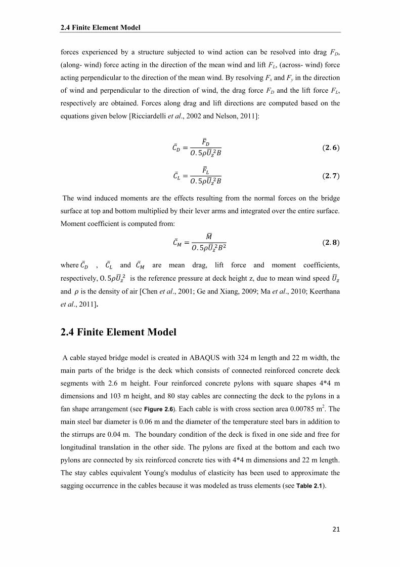
2.4 Finite Element Model
21
forces experienced by a structure subjected to wind action can be resolved into drag FD,
(along- wind) force acting in the direction of the mean wind and lift FL, (across- wind) force
acting perpendicular to the direction of the mean wind. By resolving Fx and Fy in the direction
of wind and perpendicular to the direction of wind, the drag force FD and the lift force FL,
respectively are obtained. Forces along drag and lift directions are computed based on the
equations given below [Ricciardelli et al., 2002 and Nelson, 2011]:
( )
( )
The wind induced moments are the effects resulting from the normal forces on the bridge
surface at top and bottom multiplied by their lever arms and integrated over the entire surface.
Moment coefficient is computed from:
( )
where , and are mean drag, lift force and moment coefficients,
respectively, is the reference pressure at deck height z, due to mean wind speed
and is the density of air [Chen et al., 2001; Ge and Xiang, 2009; Ma et al., 2010; Keerthana
et al., 2011].
2.4 Finite Element Model A cable stayed bridge model is created in ABAQUS with 324 m length and 22 m width, the
main parts of the bridge is the deck which consists of connected reinforced concrete deck
segments with 2.6 m height. Four reinforced concrete pylons with square shapes 4*4 m
dimensions and 103 m height, and 80 stay cables are connecting the deck to the pylons in a
fan shape arrangement (see Figure 2.6). Each cable is with cross section area 0.00785 m2. The
main steel bar diameter is 0.06 m and the diameter of the temperature steel bars in addition to
the stirrups are 0.04 m. The boundary condition of the deck is fixed in one side and free for
longitudinal translation in the other side. The pylons are fixed at the bottom and each two
pylons are connected by six reinforced concrete ties with 4*4 m dimensions and 22 m length.
The stay cables equivalent Young's modulus of elasticity has been used to approximate the
sagging occurrence in the cables because it was modeled as truss elements (see Table 2.1).

2.4 Finite Element Model
22
Table 2.1 Material properties
Material Mass density Kg/m3
Young's modulus of Elasticity Pa Poisson's ratio
High strength concrete
2643
3.10E+10
0.25
Steel bar 7800 2.00E+11 0.30
Stay cable 9438 1.65E+11 0.30
The deck is modeled as (C3D10: A10-quadratic tetrahedron) elements, pylons and ties are
modeled as (C3D8R: An 8 node linear brick reduced integration hourglass control) elements,
the reinforcing steel bars are modeled as (B31: A 2- node linear beam in space) elements and
the stay cables are modeled as (T3D2: A 2- node linear 3D truss) elements.
2.4.1 Mesh Convergence
Sufficiently refined mesh is important to make sure that the results obtained from ABAQUS
simulations are suitable. Coarse meshes can yield inaccurate results in analyses using implicit
or explicit methods. The numerical solutions of the models will tend toward a unique value as
the mesh is refined. The mesh will be converged when additional mesh refinement produces a
negligible change in the results. Mesh convergence was performed supporting on the results
of the natural frequencies for eight mode shapes of vibrations. A uniform mesh refinement
was considered with equal element size for each element type, where the results are calculated
14 times. The mesh convergence obviously starts with constant path approximately from
250000 elements (see Figure 2.4).
Figure 2.4 Mesh convergence considering four mode shapes of vibrations
1 1.5 2 2.5 3 3.5 4 4.5 5 5.5 6x 10⁵
0.1
0.2
0.3
0.4
0.5
0.6
0.7
0.8
0.9
Number of Elements
Natu
ral F
requ
ency
[ Hz
]
Mode shape 1Mode shape 3Mode shape 5Mode shape 8

2.4 Finite Element Model
23
To create the model of the cable stayed bridge, the total of 391577 elements were used
consisting of (10872-C3D8R elements, 108125-C3D10 elements, 6088-T3D2 elements and
266492-B31elements) which fall in the convergence region with finer mesh size.
2.4.2 Wind Load A strong wind with design speed of 47 m/s has been dedicated in the numerical simulations,
and the frequency of the excitation is arranged to produce vertical and torsional vibration
modes in the frequency ranges fall between the first eight mode shapes of vibrations of the
cable stayed bridge. The wind pressure assigned in the simulations is with duration of 30
seconds (see Figure 2.5). The wind fluctuation data has been prepared depending on exact data
from the literature in addition to modification of the excitation frequency [Wang et al., 2010].
Figure 2.5 Wind speed fluctuation time history
The cable stayed bridge model is divided into five regions over its height by taking in
account the wind pressure variation due to elevation from the ground. The wind pressure is
designed to excite the cable stayed bridge model perpendicular to the longitudinal axis
without skewedness. The wind forces (lift and drag) and moment are assigned to the cable
stayed bridge regions as pressure values supporting on the level of each region along the
height (see Figure 2.6).
Figure 2.6 Wind pressure and the FE model
0 5 10 15 20 25 30-1
-0.8
-0.6
-0.4
-0.2
0
0.2
0.4
0.6
0.8
t [ s ]
Wind
spee
d flu
ctuat
ion [
m/s
]

2.4 Finite Element Model
24
2.4.3 Frequency Analysis
To analyze the predicted types of vibrations of the cable stayed bridge model, frequency
analysis is conducted using ABAQUS FE program. The mode shapes of vibrations are being
calculated so that to identify the dominant mode shapes of vibrations and to confirm the
occurrence of vertical and torsional vibrations in the deck. The mode shapes of vibrations
with low frequencies are more prone to occur than the rest mode shapes with high frequencies
due to the nature of the actual winds except the situations of strong winds.
2.4.4 Results of Mode Shapes
The first 8 mode shapes of vibrations have been obtained, the type of vibration and the
related frequency were determined for each mode shape. The first 4 mode shapes are vertical
vibrations modes and their frequencies are 0.242 Hz, 0.347 Hz, 0.509 Hz and 0.613 Hz
respectively (see Table 2.2).
Table 2.2
Modes and frequencies
The fifth and sixth mode shapes are coupled lateral torsional and vertical torsional vibrations
with frequencies 0.655 Hz and 0.776 Hz respectively. While in the seventh and eighth mode
shapes are torsional and vertical vibrations respectively.
Mode shape Type Eigenvalue Frequency ( Hz )
1
2
3
4
5
6
7
8
Vertical
Vertical
Vertical
Vertical
Lateral –Torsional
Vertical – Torsional
Torsional
Vertical
2.311
4.764
10.248
14.842
16.941
23.817
24.612
26.131
0.242
0.347
0.509
0.613
0.655
0.776
0.789
0.813
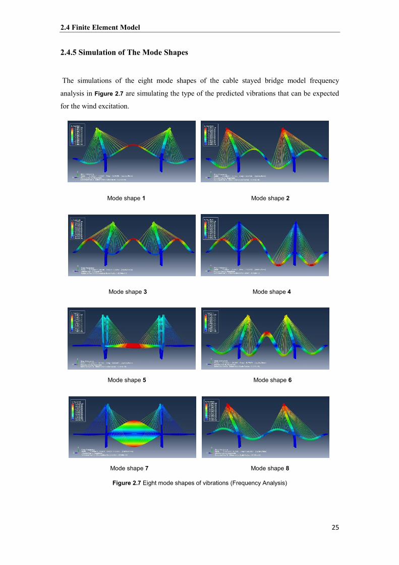
2.4 Finite Element Model
25
2.4.5 Simulation of The Mode Shapes
The simulations of the eight mode shapes of the cable stayed bridge model frequency
analysis in Figure 2.7 are simulating the type of the predicted vibrations that can be expected
for the wind excitation.
Mode shape 1 Mode shape 2
Mode shape 3 Mode shape 4
Mode shape 5 Mode shape 6
Mode shape 7 Mode shape 8
Figure 2.7 Eight mode shapes of vibrations (Frequency Analysis)

2.5 Aerodynamic Instability Analysis
26
The displacements are shown obviously and the colors are representing the magnitude of the
displacements in each point on the cable stayed bridge structure. The scale factor has been
magnified automatically by ABAQUS so that to thoroughly express on the type of vibrations
and their effect on the structural response.
2.5 Aerodynamic Instability Analysis A strong wind excitation on the cable stayed bridge is modeled with duration of 30 seconds.
The selected case for the aerodynamic parameters is the situation where the wind attack angle
value is 30°, the deck streamlined length is 1.14 m and the stay cables viscous damping is
0.0086 N.s/m. Numerical simulation is conducted for this model and data are collected for the
buffeting response and flutter instability of the structural model. 2.5.1 Results of Vertical Vibrations The vertical displacements at the mid span center of the deck are varying with time during 30
seconds of the numerical simulation. The first 7 seconds, the displacements do not exceed
0.008 m, but after that region the deck starts to vibrate stronger, and the vertical displacement
of the deck reaches 0.03 cm. This is an indication that the vertical buffeting deck response
exists and the frequency of the vibration is 0.5 Hz approximately calculated using the graph
of the vertical displacement time history of the deck center to calculate the number of the
cycles per time (see Figure 2.8). As a result it is realized that the third vertical mode shape of
vibration is dominant in this case where the natural frequency of this mode is 0.509 Hz.
Figure 2.8 Time history of vertical vibration at mid-span center of the deck
0 5 10 15 20 25 30 35-0.05
-0.04
-0.03
-0.02
-0.01
0
0.01
0.02
t [ s ]
d [ m
]

2.5 Aerodynamic Instability Analysis
27
2.5.2 Results of Torsional Vibrations
The torsional displacements at the mid span outer edges of the deck are varying with time
during 30 seconds of the numerical simulation. The first 8 seconds, the displacements do not
exceed 0.023 m which means that flutter is not obvious, but after that area the deck starts to
flutter rapidly every 1 second with a maximum torsional displacement of 0.05 m till 27
seconds of the numerical simulation. This is an indication that the torsional flutter of the deck
exists and the frequency of the vibration is 0.72 Hz approximately calculated using the graph
of the vertical displacement time history of the deck left edge to calculate the number of the
cycles per time (see Figure 2.9). This certifies that the sixth coupled vertical-torsional mode
shape of vibration is dominant in this case where the natural frequency of this mode is 0.776
Hz.
Figure 2.9 Time history of flutter vibration at mid-span edges of the deck
2.5.3 Simulation of Aerodynamic Instability To confirm the existence of aerodynamic instability in the cable stayed bridge model excited
by a strong wind, the following eight figures of the numerical simulation which have been
detailed in previous section, are being discussed (see Figure 2.10).
T = 9 s t = 11.8 s
0 5 10 15 20 25 30 35-0.04
-0.03
-0.02
-0.01
0
0.01
0.02
0.03
0.04
0.05
t [ s ]
d [ m
]

2.5 Aerodynamic Instability Analysis
28
t = 12 s t= 12.4 s
t = 12.9 s t = 14.4 s
t = 23 s t = 23.6 s
Figure 2.10 Eight simulations of vibration in the cable stayed bridge model
The first simulation at time 9 seconds shows the generation of torsional vibration in the
middle part of the deck only, where the colors are indicating this fact due to graduation of
colors in one edge only. The second simulation at time 11.8 seconds displays the additional
generation of torsional vibration in the left and right parts of the deck. The third simulation at
time 12 seconds indicates the occurrence of vertical vibration in the left part (regular
distribution of color) beside the torsional vibration of the center part of the deck. The fourth
simulation at time 12.4 seconds proofs the generation of vertical vibration of the center part of
the deck only (regular distribution of the color). The fifth simulation at time 12.9 seconds
exhibits the generation of vertical vibration at the left part of the deck. The sixth simulation at
time 14.4 seconds shows up occurrence of torsional vibrations in all parts of the deck like the
situation of the second simulation but in the opposite side. The seventh simulation at time 23
seconds features the generation of torsional vibration in the center part and vertical vibration
in right part of the deck like the third simulation but in the opposite side. Finally the eighth
simulation at time 23.6 seconds reveals the occurrence of a different torsional

2.6 Aerodynamic Parameters Optimization
29
vibration between the right and left sides of the center part of the deck. This is a firm fact on
that the buffeting vertical response and the flutter torsional instability of the deck pour into
the fact of existence of aerodynamic instability of the cable stayed bridge due to strong wind
excitation.
2.6 Aerodynamic Parameters Optimization Three aerodynamic parameters are utilized to realize their effects on the vertical vibration
and the torsional vibration of the deck in a cable stayed bridge model. Optimization of these
parameters is conducted to identify the optimum values that are taking part in the
aerodynamic stability of the cable stayed bridge, this by decreasing both the buffeting
response and the flutter instability of the structure. The first aerodynamic parameter (wind
attack angle) is the source of fluctuation of wind excitation that generates the buffeting
response in the cable stayed bridge directly, and the second aerodynamic parameter (deck
streamlined length) is responsible of the generation of both vertical and torsional vibration of
the deck due to vortex shedding incidence, and the third aerodynamic parameter (stay cables
viscous damping) is related to the control of the stay cables oscillation which takes part in the
aerodynamic stability of the cable stayed bridge. (Table 2.3) shows the range values of each
aerodynamic parameter. Table 2.3
Aerodynamic parameters and range values
In order to evaluate the effects of the three aerodynamic parameters on the vertical and
torsional vibrations of deck, nine models are utilized for the optimization process. Three cases
for each aerodynamic parameter are considered, and ABAQUS numerical simulations are
being adopted for the wind excitation on the cable stayed bridge model for a duration of 30
seconds.
Aerodynamic parameter First value Second value Third value
Wind attack angle (°)
Deck streamlined length (m)
Stay cables viscous damping ( N.s /m )
0
0
0.005
22.5
1
0.0075
45
2
0.01

2.6 Aerodynamic Parameters Optimization
31
2.6.1 Results of Wind Attack Angle Effect
When increasing the wind attack angle parameter in the FE model three times, starting from
0°, 22.5° and 45°, the displacement at the center of the deck mid-span will increase in a linear
way approximately to higher values. The effect of this parameter starts to appear from the
beginning of the wind excitation and continues in the same pattern till the end of the 30
seconds of the numerical simulation, where the maximum displacement at the center of the
deck mid span reaches 0.04 m after 16 seconds for the wind attack angle of 45° and for wind
attack angle 22.5° reaches 0.03 m, but for wind attack angle 0° is 0.02 m (see Figure 2.11).
This behavior means that increasing the wind attack angle will increase the vertical vibration
of the deck. While increasing this parameter from 0°, 22.5°and 45° will increase the flutter
displacement of the deck (outer edges) reaching to 0.042 m for wind attack angle 45° and
reaches 0.05 m both for wind attack angles 22.5° and 0° after 27 seconds of the wind
excitation. The speed of repeated fluttering of the deck starts obviously after 8 seconds and
continues till 27 seconds of the numerical simulation and the speed of the flutter occurrence
increases with the increase of the wind attack angle (see Figure 2.12).
Figure 2.11 Wind attack angle effect on the vertical displacement of the deck
Figure 2.12 Wind attack angle effect on the torsional displacement of the deck
0 5 10 15 20 25 30 35-0.08
-0.06
-0.04
-0.02
0
0.02
t [ s ]
d [ m
]
Wind attack angle 0 degreesWind attack angle 22.5 degreesWind attack angle 45 degrees
0 5 10 15 20 25 30 35-0.04
-0.02
0
0.02
0.04
0.06
t [ s ]
d [ m
]
Wind attack angle 0 degreesWind attack angle 22.5 degreesWind attack angle 45 degrees

2.6 Aerodynamic Parameters Optimization
31
2.6.2 Results of Deck Streamlined Length Effect
Increasing the deck streamlined length parameter in the FE model three times, starting from
0.0 m, 1.0 m and 2.0 m, the displacement at the center of the deck mid-span will decrease to
lower values. The effect of this parameter starts to appear after 7 seconds of the wind
excitation and continues in the same pattern till the end of the 30 seconds of the numerical
simulation. The maximum displacement at the center of the deck mid span reaches 0.0275 m
after 28 seconds for the deck streamlined length of 0.0 m and for deck streamlined length 1.0
m reaches 0.0225 m, but for deck streamlined length 2.0 m is 0.02 m (see Figure 2.13). This is
an indication that adopting streamlined sections for the deck will decrease the vertical
vibration of the deck. While increasing this parameter from 0.0 m, 1.0 m and 2.0 m will have
a very small non appreciable effect on the flutter displacement of the deck reaching to 0.05 m
for all cases approximately after 27 seconds of the wind excitation. The speed of repeated
fluttering of the deck starts obviously when after 8 seconds and continues till 27 seconds of
the numerical simulation as for wind attack angle cases, and the speed of the flutter
occurrence stays stable when increasing the deck streamlined length (see Figure 2.14).
Figure 2.13 Deck streamlined length effect on the vertical displacement of the deck
Figure 2.14 Deck streamlined length effect on the torsional displacement of the deck
0 5 10 15 20 25 30 35-0.05
-0.04
-0.03
-0.02
-0.01
0
0.01
t [ s ]
d [ m
]
Deck streamlined length 0.0 mDeck streamlined length 1.0 mDeck streamlined length 2.0 m
0 5 10 15 20 25 30 35-0.04
-0.02
0
0.02
0.04
0.06
t [ s ]
d [ m
]
Deck streamlined length 0.0 mDeck streamlined length 1.0 mDeck streamlined length 2.0 m

2.6 Aerodynamic Parameters Optimization
32
2.6.3 Results of Stay Cables Viscous Damping Effect
This time when increasing the stay cables viscous damping in the FE model three times,
starting from 0.005, 0.0075 and 0.01, the displacement at the center of the deck mid-span will
decrease in a small range with irregular pattern. The effect of this parameter starts to appear
after 6 seconds of the wind excitation and continues in the different patterns from a stable to
increasing and decreasing again during the 30 seconds of the numerical simulation. The
maximum displacement at the center of the deck mid span reaches 0.032 after 19 seconds for
the stay cables viscous damping of 0.0075 N.s/m and for stay cables viscous damping 0.005
N.s/m reaches 0.025, but for stay cables viscous damping 0.01 N.s/m is 0.025 too (see Figure
2.15). A nonlinear behavior exists due to variation of the stay cables viscous damping values
in relation with the vertical vibrations of the deck.
Figure 2.15 Viscous damping of stay cables effect on the vertical displacement of the deck
Considering torsional vibration of the deck, when increasing this parameter from 0.005 to
0.0075 and to 0.01 will have a very small non appreciable effect on the flutter displacement of
the deck for all cases but just for a period of time between 23-28 seconds reaching to
maximum 0.0475 m for both 0.005 and 0.01 cases approximately and becomes 0.0425m for
0.0075 case. The speed of repeated fluttering of the deck starts obviously after 8 seconds and
continues till 27 seconds of the numerical simulation, and the speed of the flutter occurrence
increases with the increase of the stay cables viscous damping (see Figure 2.16).
0 5 10 15 20 25 30 35-0.06
-0.05
-0.04
-0.03
-0.02
-0.01
0
0.01
0.02
t [ s ]
d [ m
]
Stay cables viscous damping 0.005 N.s/mStay cables viscous damping 0.0075 N.s/mStay cables viscous damping 0.01 N.s/m

2.7 Validation of The FE Models
33
Figure 2.16 Viscous damping of stay cables effect on the torsional displacement of the deck
2.7 Validation of The FE Models
The lift and moment coefficients calculated for the deck models are validated with two
benchmarks from the latest literature. First benchmark is the results obtained from the flat
plate theory and the second benchmark is the results of the flat plate model collected from
experiments done by (Xavier et al. 2015). (Table 2.4) shows the data of the lift coefficient
and moment coefficient for the two benchmarks and the numerical analysis results
calculated from the ABAQUS FE models.
Table 2.4
Results of lift and moment coefficients for ABAQUS FE model and two benchmarks
FE model Flat plate theory FE model
Flat plate (Xavier)
Angle of attack
0°
4°
8°
12°
16°
0.070
0.480
0.640
0.660
0.620
0.000
0.450
0.700
0.740
0.680
-0.0013
0.0078
0.0154
0.0305
0.0266
-0.0015
0.0080
0.0140
0.0280
0.0250
2.7.1 Flat Plate Theory Benchmark
0 5 10 15 20 25 30 35-0.04
-0.02
0
0.02
0.04
0.06
t [ s ]
d [ m
]
Stay cables viscous damping 0.005 N.s/mStay cables viscous damping 0.0075 N.s/mStay cables viscous damping 0.01 N.s/m

2.7 Validation of The FE Models
34
There is a very good agreement between the results of the lift coefficient for the FE model
and the flat plate theory in relation with multiple wind attack angle cases as shown in Figure
2.17.
Figure 2.17 Lift coefficient with wind attack angle validation
where the curves of the data for the two approaches are in a coinciding pattern starting from
0°- 16° of wind attack angle. There is a small difference in lift coefficient value between them
which is not exceeding 0.1 for the maximum situation for the wind attack angle of 12°.
2.7.2 Flat Plate Model (Xavier and Co-authors) Benchmark The comparison between the results of the moment coefficient for the FE model and the
results of the flat plate model experiment done by by Xavier and co-authors for the wind
attack angle cases is pointing to a good agreement between them. The two curves are
coinciding to a good extent in the range of 0°-16° of wind attach angle and the maximum
difference in moment coefficient is 0.0025 at the situation of 12° wind attach angle (see
Figure 2.18).
Figure 2.18 Moment coefficient with wind attack angle validation
0 2 4 6 8 10 12 14 160
0.1
0.2
0.3
0.4
0.5
0.6
0.7
0.8
Alpha [ ° ]
Cl
Flat Plate TheoryFE model
0 2 4 6 8 10 12 14 16-0.005
0
0.005
0.01
0.015
0.02
0.025
0.03
0.035
Alpha [ ° ]
Cm
Flat Plate (Xavier et al. 2015)FE model

2.8 Sensitivity Analysis
35
2.8 Sensitivity Analysis Sensitivity analysis is the study of how the uncertainty in the output of the model can be
handed out to various sources of input, or it attributes to the identification of individual
donation and various origins of uncertain inputs to the uncertainty in the output of a model
[Saltelli et al., 2000; Saltelli, 2004; Saltelli et al., 2008; Keitel et al., 2011]. There are two
sorts of sensitivity analysis methods: local sensitivity analysis and global sensitivity analysis.
Local sensitivity analysis methods calculate or convergent the local response of the model
outputs through modifying input parameters or individual parameters with other parameters at
nominal values in the hyperspace of the input parameter. In the other hand, global sensitivity
analysis estimates the effects of input variations on the outputs in the total permitted ranges of
the input space [Confalonieri et al., 2010; Tong, 2010; Zhan et al., 2013; Baroni and
Tarantola, 2014].
Analyses involve the consideration of models of the form: = ( ) where = [ 1, ,….,
] is a vector of analysis result and = [ , ,…. , ] is a vector of imprecisely known
analysis inputs. In general the model f can be quite large and involved (e.g., a system of
nonlinear partial differential equations requiring numerical solution or possibly a sequence of
complex, linked models as is the case in a probabilistic risk assessment for a nuclear power
plant or a performance assessment for a radioactive waste disposal facility the vector of
analysis results can be of high dimension and complex structure (e.g., the elements of might
be several hundred temporarily or spatially dependent functions); and the vector of analysis
inputs can also be of high dimension and complex structure e.g., several hundred variables,
with some variables corresponding to physical properties of the system under study and other
variables corresponding to parameters in probability distributions or perhaps to designators
for alternative models. The uncertainty in the elements of is characterized by a sequence of
probability distributions. where is a probability distribution characterizing
the uncertainty in [Saltelli, 2004; Storlie and Helton, 2008; Wainwright et al., 2014].
2.9 Experimental Design
Experimental design is widely used to control the effects of parameters in many problems.
The use of this method decreases the number of experiments, using time and material
resources. Furthermore, the experimental errors are minimized and the analysis performed on
the results is easily realized. Utilizing experimental design, the statistical methods measure
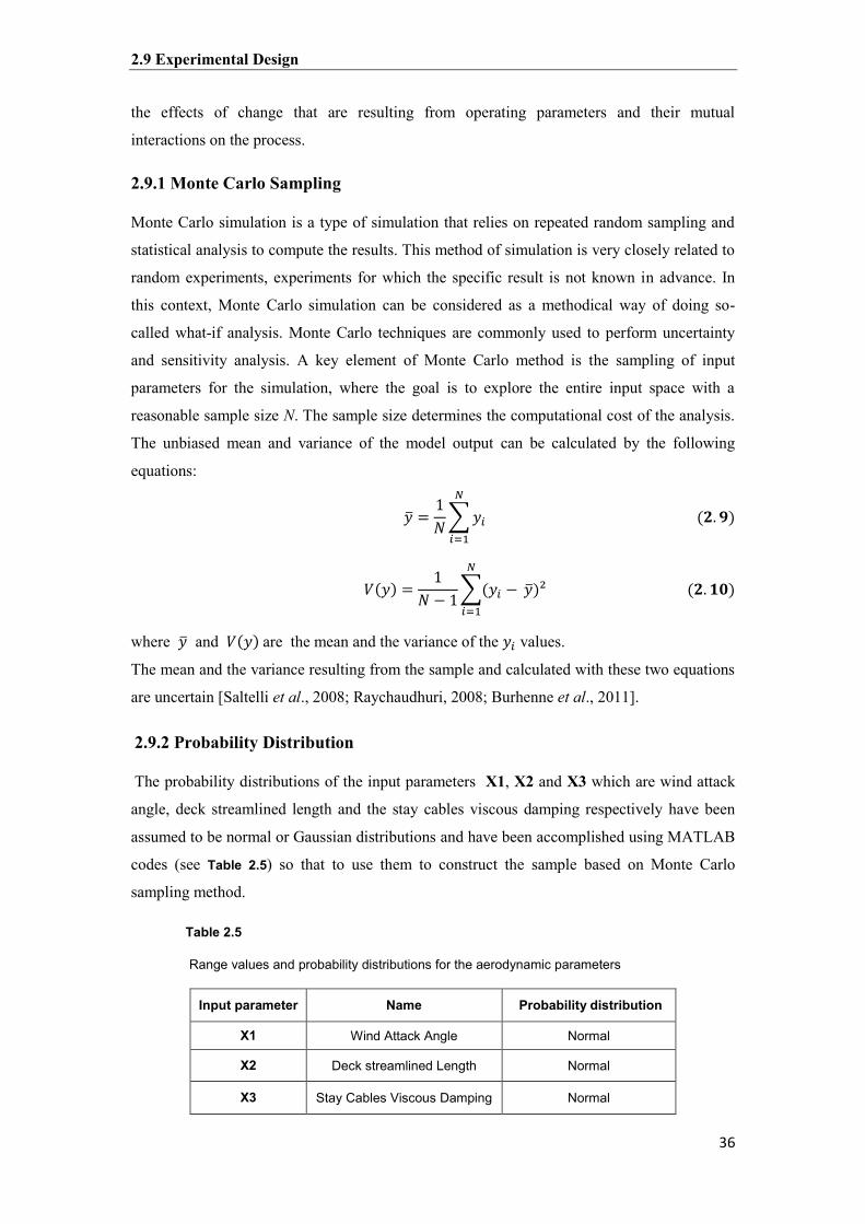
2.9 Experimental Design
36
the effects of change that are resulting from operating parameters and their mutual
interactions on the process.
2.9.1 Monte Carlo Sampling Monte Carlo simulation is a type of simulation that relies on repeated random sampling and
statistical analysis to compute the results. This method of simulation is very closely related to
random experiments, experiments for which the specific result is not known in advance. In
this context, Monte Carlo simulation can be considered as a methodical way of doing so-
called what-if analysis. Monte Carlo techniques are commonly used to perform uncertainty
and sensitivity analysis. A key element of Monte Carlo method is the sampling of input
parameters for the simulation, where the goal is to explore the entire input space with a
reasonable sample size N. The sample size determines the computational cost of the analysis.
The unbiased mean and variance of the model output can be calculated by the following
equations:
∑
( )
( )
∑(
) ( )
where and ( ) are the mean and the variance of the values.
The mean and the variance resulting from the sample and calculated with these two equations
are uncertain [Saltelli et al., 2008; Raychaudhuri, 2008; Burhenne et al., 2011]. 2.9.2 Probability Distribution The probability distributions of the input parameters X1, X2 and X3 which are wind attack
angle, deck streamlined length and the stay cables viscous damping respectively have been
assumed to be normal or Gaussian distributions and have been accomplished using MATLAB
codes (see Table 2.5) so that to use them to construct the sample based on Monte Carlo
sampling method.
Table 2.5
Range values and probability distributions for the aerodynamic parameters
Input parameter Name Probability distribution
X1 Wind Attack Angle Normal
X2 Deck streamlined Length Normal
X3 Stay Cables Viscous Damping Normal
2.9 Experimental Design
37
The aerodynamic parameters X1, X2 and X3 are arranged in samples according to the Monte
Carlo sampling method. These samples are used to determine the predicted vertical and
torsional displacements both at the center and outer edges of the deck mid-span respectively,
so that to formulate the surrogate models for upcoming sensitivity analysis.
2.9.3 Response Surface Methodology
Response surface methodology is a set of statistical and mathematical methods being used
for the analysis and modeling of many problems in the engineering field. The main purpose of
this methodology is to optimize the response surface which is being influenced by various
parameters. This methodology quantifies the relationship between the obtained response
surfaces and the controllable input parameters.
If all variables are assumed to be measurable, the response surface can be expressed as
follows:
( ) ( )
where is the answer of the system, and the variables of action called factors. The goal is
to optimize the response variable . It is assumed that the independent variables are
continuous and controllable by experiments with negligible errors. It is required to find a
suitable approximation for the true functional relationship between independent variables and
the response surface. Two important models are utilized in response surface methodology, the
first-degree model which is represented as follows:
∑
( )
and the second-degree model is formulated in the following equation:
∑
∑
∑∑
( )
where , , . . . , are the input factors which influence the response ; (
) (i = 1, 2,. . . ,k), (i = 1, 2, . . . ,k; j = 1, 2,. . . ,k) are unknown parameters
and is a random error. The coefficients are obtained by the least square method.
a series of n experiments should first be carried out, in each of which the response is
measured (or observed) for specified settings of the control variables. The totality of these

2.9 Experimental Design
38
settings constitutes the so-called response surface design, or just design, which can be
represented by a matrix, denoted by D, of order n × k called the design matrix,
(
)
( )
where denotes the u th design setting of (i = 1, 2, . . . , k; u = 1, 2, . . . , n). Each row of
D represents a point, referred to as a design point, in a k -dimensional Euclidean space. Let
denote the response value obtained as a result of applying the u th setting of x, namely
= ( , , . . . , ), (u = 1, 2, . . . , n).
In general:
( )
where = ( , , . . . , ) which is defined as a matrix of measured values, is a matrix of
independent variables of order n × p whose u th row is ( ), and ϵ = (ϵ , ϵ , . ………. . ,
ϵ ). Note that the first column of is the column of ones 1n.
Assuming that has a zero mean, the so called ordinary least-squares estimator of β is:
( ) ( )
where is the transpose of the matrix and ( ) is the inverse of the matrix
[Gunaraj and Murugan, 1999; Annadurai et al., 2004; Kwak, 2005; Aslan and Cebeci, 2007;
Amenaghawon et al., 2013].
2.9.4 Sobol’s Sensitivity Indices
Sobol’s indices are a global sensitivity measures which determine the contribution of each
parameter (or group of parameters) to the variance of the output. The usual Sobol’s sensitivity
indices include the main and total effects for each parameter, but the method can also provide
specific interaction terms [Glen and Isaacs, 2012]. It uses a variance ratio to estimate the
importance of parameters. This method is based on the partitioning of the total variance of
model output V(Y) using the following equation:
( ) ∑
∑
∑
( )

2.9 Experimental Design
39
where represent the first order effect for each parameter ( – [ ( | )]) and :
( ( | )) – ) to is the interactions among parameters. The first-
order sensitivity index can be calculated by:
( )
[ ( | )]
( ) ( )
where [ ( | )] is the variance of the expected value of when conditioning with respect
to and ( ) is the unconditional variance of
and the second-order sensitivity index can be calculated by:
( ) [ ( | )]
( ) ( )
In general, the total sensitivity index can be defined as [Homma and Saltelli, 1996;
Saltelli and Tarantola, 2002; Saltelli and Annoni, 2010]:
( ( | ))
( ) ( )
where the subscript refers to all of the inputs except input , Also the total sensitivity
index can be written as:
( ( | ))
( ) ( )
where ( ( | )) is the variance of the expected value of when conditioning with
respect to all parameters except for .
Due to parameter interaction of a parameter increases, therefore Ʃ ≥ 1 will always
hold. The difference – is a measure of how much interacts with other input
parameters.
The index is therefore a measure of the exclusive influence of input parameter If the
sum of all is close to one, the model is additive with respect to its variances and no
remarkable interactions between the parameters seem to exist [Nossent et al., 2011; Keitel et
al., 2011; Zhan et al., 2013; Baroni and Tarantola, 2014; Zhang et al., 2015].
2.9.5 Results and Discussion of The Surrogate Models
The regression coefficients calculated both for vertical and torsional actual displacements
supported on Monte Carlo experimental method, and in order to formulate the surrogate
models for the predicted vertical and torsional displacements, 400 samples were used
considering convergence process between the sensitivity indices. Quadratic and interaction

2.9 Experimental Design
41
terms were used to construct he surrogate model for the case of vertical displacement at the
center of the deck mid-span. The calculated coefficient of determination R2 between the actual
and the predicted vertical displacements was 98.12% (see Figure 2.19) which is an excellent
representation of the predicted vertical displacement, which means that just 1.88% of the
system response still unexplained.
Figure 2.19 Coefficient of determination between actual and predicted vertical displacement
The following response surface plots in Figure 2.20, Figure 2.21 and Figure 2.22 which have
been generated using MATLAB codes, are the relation between each two aerodynamic
parameters X1X2, X1X3, X2X3 and the predicted vertical displacement at the center of the
deck mid span.
Figure 2.20 Response surface plot showing effect of X1 and X2 on the predicted vertical displacement
0.0202 0.0203 0.0203 0.0204 0.0204 0.0204 0.0205 0.0205 0.0206 0.02060.0202
0.0203
0.0203
0.0204
0.0204
0.0204
0.0205
0.0205
0.0206
0.0206
VD - actual [ m ]
VD -
pred
icte
d [ m
]
R2=0.9812
010
2030
4050
11.2
1.41.6
1.82
-0.028
-0.026
-0.024
-0.022
-0.02
X1 Angle of attack °X2 Deck streamlined length m
Pred
icte
d v
ertic
al d
ispla
cem
ent
m

2.9 Experimental Design
41
Figure 2.21 Response surface plot showing effect of X1 and X3 on the predicted vertical displacement
Figure 2.22 Response surface plot showing effect of X2 and X3 on the predicted vertical displacement
Quadratic and interaction terms were used to build the surrogate model to calculate the
torsional displacement at the outer edges of the deck mid-span. The coefficient of
determination R2calculated between the actual and the predicted torsional displacements was
R2 = 97.50 % which is a very good approximation for the prediction of torsional displacement
that only 2.50 % of the system response remains unexplained (see Figure 2.23).
Figure 2.23 Coefficient of determination between actual and predicted torsional displacement
2 2.1 2.2 2.3 2.4 2.5 2.6 2.7 2.8x 10⁻³
1.9
2
2.1
2.2
2.3
2.4
2.5
2.6
2.7
2.8x 10⁻³
TD - actual [ m ]
TD -
pred
icted
[ m
] R2=0.9750
010
2030
4050
56
78
910
x 10-3
-0.023
-0.022
-0.021
-0.02
-0.019
X1 Angle of attack °X3 Stay cables viscous damping
Pred
icte
d ve
rtic
al d
ispla
cem
ent
m
11.2
1.41.6
1.82 5
678910 x 10-3
-0.023
-0.0225
-0.022
-0.0215
-0.021
-0.0205
-0.02
X3 Stay cables viscous dampingX2 Deck streamlined length m
Pred
icte
d v
ertic
al d
ispla
cem
ent
m

2.9 Experimental Design
42
The following response surface plots express on the relation between each two aerodynamic
parameters X1X2, X1X3, X2X3 and the predicted torsional displacement at the outer edges of
the deck mid span is shown in Figure 2.24, Figure 2.25 and Figure 2.26 which have been
generated using MATLAB codes.
Figure 2.24 Response surface plot showing effect of X1 and X2 on the predicted torsional displacement
Figure 2.25 Response surface plot showing effect of X1 and X3 on the predicted torsional displacement
Figure 2.26 Response surface plot showing effect of X2 and X3 on the predicted torsional displacement
010
2030
4050
11.2
1.41.6
1.820
0.5
1
1.5
2
2.5x 10-3
X1 Angle of attack °X2 Deck streamlined length m
Pred
icte
d to
rsio
nal
disp
lace
men
t m
010
2030
4050
56
78
910
x 10-3
1.5
2
2.5
3
3.5
4x 10-3
X1 Angle of attack °X3 Stay cables viscous damping
Pred
icte
d to
rsio
nal
disp
lace
men
t m
11.2
1.41.6
1.82
56
78
910
x 10-3
1.5
2
2.5
3x 10-3
X2 Deck streamlined length mX3 Stay cables viscous damping
Pred
icte
d to
rsio
nal
disp
lace
men
t m

2.9 Experimental Design
43
2.9.6 Results and Discussion of The Sensitivity Indices
The main orders of sensitivity indices for each aerodynamic parameter in addition to their
interaction orders were calculated considering the convergence results which recommended
using 400 samples to calculate both the vertical displacement and torsional displacement at
the center and the outer edges of the mid span of the cable stayed bridge model respectively
(see Figure 2.27 and Figure 2.28). Supporting on the calculated results, the total sensitivity
indices for each aerodynamic parameter have been calculated (see Table 2.6).
Table 2.6
Sensitivity indices of the aerodynamic parameters
Sensitivity indices Vertical displacement
Torsional displacement
first order X1
first order X2
first order X3
sum of first orders
interaction between X1 and X2
interaction between X1 and X3
interaction between X2and X3
total order of X1
total order of X2
total order of X3
sum of total orders
0.682520
0.154241
0.129080
0.965841
0.011241
0.008712
0.000537
0.702473
0.166019
0.138329
1.006821
0.557385
0.236873
0.205698
0.999956
0.000107
0.000044
0.000082
0.557536
0.237062
0.205824
1.000422
In relation with the vertical displacement , the total order sensitivity index of aerodynamic
parameter (wind attack angle) is 0.7024, this value is bigger than the total order sensitivity
index of aerodynamic parameter (deck streamlined length) X2 which is 0.1660, also it is
bigger than the total order sensitivity index of aerodynamic parameter (stay cables viscous
damping) X3 which is 0.1383, this means that the vertical displacement is 70.24% due to
variation in the wind attack angle, and it is 16.60% due to the variation in the deck
streamlined length. Also it is 13.83% due to the variation in the stay cables viscous damping.
While the interaction index between the aerodynamic parameters X1 and X2 is 0.0112 and
between X1 and X3 is 0.0087, while between X2 and X3 is 0.0005, which means that there is

2.9 Experimental Design
44
a small interaction between the aerodynamic factors taking part in the variation of the vertical
displacement of the deck at the center of the mid span.
While considering the torsional displacement , the total order sensitivity index of X1 is
0.5575, which is the biggest aerodynamic parameter which is bigger twice of the total order
sensitivity index of X2 which is 0.2370 approximately, also it is bigger twice the total order
sensitivity index of X3 which is 0.2058 approximately, this means that the torsional
displacement is dependable 55.75% on the wind attack angle variation, while it is 23.70%
due to the deck streamlined length variation, and it is 20.58% due to the variation in stay
cables viscous damping. While the interaction index between X1 and X2 is 0.0001 and
between X1 and X3 is 0.0000, in the other hand, between X2 and X3 is 0.0000 too, this
proofs that the surrogate model is additive approximately which means that there is no
interaction between aerodynamic parameters take part in the variation of the torsional
displacement of the deck at the outer edges of the mid span.
2.9.7 Convergence of The Results
The process of global sensitivity analysis supporting on Sobol's sensitivity indices requires
certain or adequate samples of experiments to find out the predicted effect of the aerodynamic
parameters on the response of the system. The most efficient number of samples is being
identified through the convergence of the sum of first orders and total sensitivity indices of
the aerodynamic parameters. All the sensitivity indices (first orders, interaction orders and
total orders) for each aerodynamic parameter have been calculated using m MATLAB codes.
Two outputs have been utilized in the process of converges, the vertical displacement and
torsional displacement. Figure 2.27 and Figure 2.28 show the relation between the number of
samples and the sum of first orders sensitivity indices, in the same time between the number
of samples and the sum of total sensitivity indices of the three aerodynamic parameters.
Figure 2.27 Convergence of sensitivity indices –Vertical displacement
0 100 200 300 400 500 600 7000.94
0.95
0.96
0.97
0.98
0.99
1
1.01
1.02
1.03
Ns
Si
Sum of first orders sensitivity indicesSum of total orders sensitivity indices

2.9 Experimental Design
45
For the case of vertical displacement (see Figure 2.27), the two curves of the sum of first
orders and total orders of sensitivity indices at the beginning are not coinciding to reach
convergence till 400 samples. After this stage the two curves are starting to converge at the
400 number of samples, where the two curves continue to remain in a stable position after
many times of changing the number of samples.
Also for the torsional displacement (see Figure 2.28) the two curves are reaching convergence
at 400 samples too, and the coinciding pattern continues.
Figure 2.28 Convergence of sensitivity indices –Torsional displacement
The convergence results of the two cases necessitate utilizing 400 samples of experiments to
efficiently get the predicted rational effects of each aerodynamic parameter on both the
variation of the vertical displacement and torsional displacement.
0 100 200 300 400 500 600 7000.999
0.9995
1
1.0005
1.001
1.0015
1.002
1.0025
1.003
Ns
Si
Sum of first orders sensitivity indicesSum of total orders sensitivity indices

46

47
Chapter 3
Kinetic Energy Based Model Assessment
3.1 Von Karman Vortex Street Attempts have been made to obtain analytical expressions for the fluctuating lift force
experienced by the bluff cylinder owing to the ideal Karman-Benard vortex trail (see Figure
3.1). The stable configuration of vortices possesses the relations: / =
arccosh √ and | | √ , where is the strength of vorticity
for a concentrated vortex. is the speed of the vortices, is the distance between the
vortices in a row and is the distance between the rows.
Figure 3.1 Karman-Bernard’s (Von Karman) vortex street
Furthermore, it was shown that the vortex trail induces almost steady drag force to the body
given by the following formula:
( )
in which is the mean value of the induced horizontal force per unit length , is the kinetic
pressure and the associated force coefficient is expressed as:
( )
( )
Considering infinite vortex trail and circular cross-section, Chen found that:
( )

3.2 VIV Parameters
48
where
(
*
( )
is the fluctuating across-wind force per unit length and is the associated aerodynamic
exciting coefficient. The aeroelastic actions can be considered in Equation (3.2) and
Equation (3.4) by noting that the spacing between the vortex row , and thus the induced
forces, can alter, if the cross-section performs across-wind oscillations. In general, analytical
formulations for the aerodynamic exciting coefficients are dependent on the approximations
assumed for the near-wake behind the body. The vibrations generated by vortex shedding
usually occur in slender structures with low damping. The vibrations occur if the vortex
shedding frequency coincides with or come close to the natural frequency of the structure.
The vortex shedding frequency fs of a non-vibrating body can be derived as suggested by
[Dyrbye and Hansen, 1999] see Figure 3.2. The time between the vortices at each side is
equal to the distance lv divided by the speed of the vortices U1. The frequency is the inverse
of the period, giving that fs = U1/lv. The distance between the vortices lv, must be
proportional to the structure width d, since this is the only relevant length.
Figure 3.2 Vortex Street for a bluff body (Dyrbye and Hansen, 1999)
3.2 VIV Parameters
3.2.1 Reynolds Number
Reynolds number is a dimensionless number that describes the flow around smooth bluff
bodies such as a bridge deck. It is the ratio between the inertia forces and viscous forces:
( )

3.2 VIV Parameters
49
in which is the diameter of the cylinder, is the flow speed and is the kinematic
viscosity of the fluid. Flow regimes are obtained as the result of many changes of the
Reynolds number. The changes of the Reynolds number generate separation of flows in the
wake region of the bluff body, which are called vortices. At low values of Reynolds number
( < 5), there no separation occurs. When Reynolds number is further increased, the
separation starts to occur and becomes unstable and initiates the phenomenon named vortex
shedding at particular frequency. The main parameter of Reynolds number is the wind speed
that is directly related to the generation of VIV by affecting the kinetic energy of the flow
system that is the source of vortex shedding [Schewe and Larsen, 1998; Kazutoshi et al.,
2007; Irwin, 2008; Asyikin, 2012; Wu and Kareem, 2012; Sutardi, 2014].
3.2.2 Deck Shape
The deck shape of a bridge is essential to be in such a way to enhance the aerodynamic
behavior and to reduce the tendency to vortex shedding. [Bienkiewicz, 1987] studied various
cross section samples and [Nagao et al, 1993] studied the ratios of width and the height of
box girders and many shapes of fairing. The results of these studies concluded that the best
streamlined deck shape involves better aerodynamic stability of the structure. While
[Wardlaw et al., 1983] discovered that the turbulence can suppress the vortex shedding.
[Noda et al., 2009] displayed the role of the leading edge of the bottom deck separation on the
lift force at a certain Reynolds number. However, there are other flow features, like top deck
leading edge separation and bottom deck trailing separation that their aerodynamic behavior
are still not clear [Larsen and Walther, 1998; Lin et al., 2005; Gosteev et al., 2014; Haque et
al., 2016].
3.2.3 Dynamic Viscosity of Air
Vortex shedding has an important relation with the dynamic viscosity of air, so it is essential
to consider this parameter in the study of vortex shedding patterns and vortices shapes. The
contact between the air particles and the deck surface has adhesion force that creates the
boundary layer. However, because of air mass, it undergoes inertial effect according to
Newton’s law and Navier-Stokes equations. The link between the inertial forces and the
viscous forces is specified by Reynolds number. The boundary layer separation point explains
the deck behavior submerged in the wind flow. A deck shape with a surface with high
curvature, the separation point modifies with respect to Reynolds number, which is the source
of diverse effects related to vortex shedding [Jurado et al., 2012 and Meinhardt et al., 2014].
The dynamic viscosity of air represents the resistance of the air to shearing wind flows. This
parameter has values that vary linearly with the variation of temperature (see Figure 3.3).

3.3 Vortex Shedding Phenomenon in Bridges
51
Figure 3.3 Dynamic viscosity of air versus temperature
3.3 Vortex Shedding Phenomenon in Bridges
When a bridge deck is subjected to a wind flow perpendicularly, the wind would be retarded
when it is with contact with the deck surface and boundary layer being composed. This
boundary layer at some parts of the deck, trends to separate from the deck. The separation of
the boundary layer generates a force on the deck and pressure on the windward part and
suction at leeward part. As a result, vortices would be formed which alters the distribution of
pressure on the bridge deck surface leading to structural deflections of the deck. These
vortices might not be symmetric around the deck. Hence diverse lifting forces are generated
around the deck. The motion of the deck would be transverse to the direction of the incoming
wind. When the shedding frequency of vortices matches the natural frequency of the bridge,
resonance oscillations will occur predominantly. The amplitude of the oscillations relies on
the system damping and the fluctuation of the wind. These oscillations might reach lock-in
region, consequently result in dangerous extension and failure due to fatigue [Zhang et al.,
2004; Diana et al., 2006; Flamand et al., 2013; Belloli et al., 2014; Grouthier et al., 2014;
Meinhardt et al., 2014].
Due to fluctuation of wind and variation with respect to time and elevation, the frequency of
vortex shedding is not remaining stable for a long time. As a result, bridges are not apt to
everyday wind excitation. In a critical case, when the wind is unusually stable and long
lasting, vortex shedding can result in vertical motion of the deck with amplitude up to
decimeters, where the duration of wind excitation in this case ranges between several minutes
and some hours. The amplitude of oscillations is an important case that is concerning the
users’ comfort, especially when it reaches noticeable level and when the fatigue of the
-20 -10 0 10 20 30 40 501.6
1.65
1.7
1.75
1.8
1.85
1.9
1.95
2x 10⁻⁵
Temp.[ °C ]
Mu
[ Pa
.s ]

3.4 Finite Element Model
51
structural elements is expected. A principal sketch of the phenomenon can be seen in Figure
3.4.
Figure 3.4 Schematic flow around a stationary bridge deck
A wind flow around asymmetric bluff body like a bridge deck will affect the periodic vortex
shedding or even suppress it. The motion of the deck which is periodic in nature may occur
when the shedding frequency of the vortices is close to natural frequency of the bridge. The
vortex induce vibrations can be averted by assigning the frequencies of the generated vortices
be widely far from the natural frequency of the bridge. This step can be done by changing the
geometry of the bridge structure or altering the natural frequencies in the design stage or after
construction. Strouhal number is the most critical parameter in the subject of vortex shedding,
which links between the shedding frequencies of the vortices, buff body diameter and flow
speed. Due to nonlinearity in the bridge structures and aerodynamic force Simiu and Scanlan,
1996 suggested a synthesis sample to take into account the nonlinear influence [Marin, 2003;
Dol et al., 2008; Stevens and Simonsen, 2008; Andrianne, 2012; Flamand et al., 2014].
3.4 Finite Element Model The bridge segmental deck model is generated in ABAQUS-CFD in 2D model with
dimensions 2.6 m height and total width of 22 m as shown in Figure 3.5, the thickness is 2 m.
The flow domain size is 140 m length and 40 m height, the position of the deck model in the
flow domain should be in a position so that to facilitate a proper area to show the vortex
shedding in the downstream Figure 3.6, in addition to an appropriate area above and under the
deck model to show the boundary layers around the deck with the separation points.

3.4 Finite Element Model
52
Figure 3.5 Deck model dimensions
Figure 3.6 Flow domain size in CFD
The air density is assigned 1.29 kg/m3 and the dynamic viscosity of the air is assigned
between the range (1.6321E-05 - 1.9821E-05) Pa.s depending on the temperature between (-
20) C° and (50) C° (see Figure 3.3). The model part is meshed using CFD element fluid
family with FC3D8: A-8 node linear fluid brick. The deck wall assigned with 0.4 element size
and the flow domain with 1 element size. A flow step with 100 seconds duration is created to
simulate the vortex shedding. Spalart- Allmaras turbulence model has been used in this
analysis for turbulent flow situations. Four boundary conditions are defined for the model,
fluid boundary B.C for the inlet flow and far fields assigning the air speed value in the
horizontal direction only (zero attack angle) and the other two directions with zero
magnitudes, fluid B.C for the outlet flow assigning zero pressure, fluid B.C for the front and
back of the flow model with zero speed magnitude for the third direction perpendicular to the
model (z- direction) and non-slip fluid B.C for the wall condition of the deck. A job is created
and the results are analyzed depending on the case if the model needs to be assigned model
turbulence or not, this is to be done by checking the time history of the kinetic energy
dissipated, where if the plot is oscillating randomly this means that the model needs to
activate the model turbulence in the flow step, as a result this indicates necessity of
predefining a fluid turbulence in the initial step. Commonly a very large number of Reynolds
number indicates the need for a turbulence model.

3.4 Finite Element Model
53
3.4.1 Mesh Convergence
The vortex shedding in the flow domain at the downstream of the deck in the velocity field
depends on the mesh size around the deck and the downstream so that to facilitate a better
simulation for the boundary layers and separation regions, in addition to the vortex shedding
periodically. Figure 3.7 shows the velocity field of the result with mesh size 28074 elements
where the vortex shedding is not simulated correctly compared to the actual phenomenon, the
vortices shedding is not in an asymmetric style, this is due to very fine mesh size around the
deck model.
Figure 3.7 Vortex shedding – Mesh size 28074 elements
The vortex shedding simulation in Figure 3.8 with mesh size 9943 elements is the best
simulation of the actual phenomenon, this is because the vortices shed is in an asymmetric
form and the shedding is near the trail of the deck at the wake region, and it worthy that the
mesh size in this case is appropriate, while the vortex shedding simulated in the model in
Figure 3.9 with mesh size 7724 elements is simulated in a weak style because the shedding of
vortices is relatively far from the trail of the deck despite the asymmetric style, and this
indicates that the mesh size is not suitable.
Figure 3.8 Vortex shedding – Mesh size 9943 elements

3.4 Finite Element Model
54
Figure 3.9 Vortex shedding – Mesh size 7724 elements
The models in Figure 3.10 and Figure 3.11 with mesh sizes 6202 and 5317 elements
simultaneously are not showing the vortex shedding at all due to the coarse mesh sizes of the
models. They look like to have a very large Reynolds number especially high speed
magnitude of the wind flow. As a result the mesh size of 9943 elements would be utilized to
mesh the CFD model.
Figure 3.10 Vortex shedding – Mesh size 6202 elements
Figure 3.11 Vortex shedding – Mesh size 5317 elements

3.5 Results of Vorticity and Kinetic Energy
55
3.5 Results of Vorticity and Kinetic Energy
3.5.1 Wind Speed Effect
When the wind speed parameter denoted by X1 increases, the vortex shedding in the
downstream of the deck is obviously being better generated and regulated in shape and the
frequency of shedding increases. When the wind speed V= 0.5 m/s, the vortex shedding is in
the way to generate and the vortices are simply shedding but without regular style (see Figure
3.12).The vorticity field of this case shows the wind flow around the deck and the start of
vortex shedding in the wake region (see Figure 3.13). When the wind speed increases to
V=12.5 m/s, the vortex shedding appears very well and the asymmetric pattern of the vortices
can be seen very well (see Figure 3.14) with bigger frequency of shedding. The vortices shape
and style in this case are bigger and wider than the previous case (see Figure 3.15). While
when the wind speed reaches V=25 m/s, the vortex shedding can be seen more organized with
bigger frequency of shedding (see Figure 3.16). The vorticity field shows bigger vortices and
different style of shedding (see Figure 3.17). All these cases indicate that increasing the wind
speed will help to better generate the vortex shedding in the wake region, also the shape and
the pattern of the vortices change to different style and the frequency of shedding increases,
where this will enhance starting the vibration of the deck.
Figure 3.12 Vortex shedding - Velocity field - V=0.5 m/s
Figure 3.13 Vortex shedding - Vorticity field - V=0.5 m/s
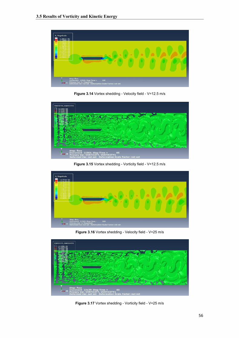
3.5 Results of Vorticity and Kinetic Energy
56
Figure 3.14 Vortex shedding - Velocity field - V=12.5 m/s
Figure 3.15 Vortex shedding - Vorticity field - V=12.5 m/s
Figure 3.16 Vortex shedding - Velocity field - V=25 m/s
Figure 3.17 Vortex shedding - Vorticity field - V=25 m/s

3.5 Results of Vorticity and Kinetic Energy
57
Regarding the kinetic energy of the system, when the wind speed increases, the kinetic
energy increases in a nonlinear way. When the wind speed is V = 0.5 m/s, the kinetic energy
starts increasing till 18 seconds from the simulation, and after that it starts to decrease in a
semi linear way due to energy dissipation due to generation of very simple vortex shedding
that can be seen in Figure 3.18. While for wind speed V = 12.5 m/s, the kinetic energy
increases till 2 seconds from the simulation and suddenly drops down till 7 seconds from the
simulation and again starts to rise until 13 seconds with an oscillatory style in the same time
decreasing to a stable oscillatory position starting from 20 seconds from the simulation till the
end indicating the start of the deck vibration with a certain frequency (see Figure 3.19).
Furthermore, when the wind speed is higher V = 25 m/s, the kinetic energy increases highly
in the same way as previous case of V = 12.5 m/s, but the sudden drop and sudden rise start in
earlier position in the same time with a greater frequency of oscillation (see Figure 3.20). The
overall comparison between the three kinetic energy cases can be seen in Figure 3.21.
Figure 3.18 Wind speed V = 0.5 m/s and the kinetic energy of the system
Figure 3.19 Wind speed V = 12.5 m/s and the kinetic energy of the system
0 20 40 60 80 100 120
9.14
9.16
9.18
9.2
9.22
9.24
9.26
9.28
t [ s ]
Ke [
N .
m ]
0 20 40 60 80 100 1205690
5700
5710
5720
5730
5740
5750
5760
t [ s ]
Ke [
N . m
]

3.5 Results of Vorticity and Kinetic Energy
58
Figure 3.20 Wind speed V = 25 m/s and the kinetic energy of the system
Figure 3.21 Effect of wind speed on the kinetic energy of the system
3.5.2 Deck Streamlined Length Effect
The input parameter X2 is the deck streamlined length. When the wind speed is constant and
just this length is changed, many situations of vortex shedding from the wake region and
vortices shapes and patterns are recognized. When this length L = 0 m, the vortex shedding is
generated in an primary establishing pattern showing the two rows of the asymmetric rows of
the vortices (see Figure 3.22), but when the length L =1 m, the vortex shedding modifies to
better shape and pattern of vortices in the two rows and the vortex trail can be recognized and
seen better (see Figure 3.23). While when this length L = 2 m, the vortex shedding disappears
and the vortices shape and pattern are destroyed (see Figure 3.24).
0 20 40 60 80 100 120-1
0
1
2
3
4x 10⁴
t [ s ]
Ke [
N .
m ]
wind speed v = 0.5 m/swind speed v = 12.5 m/s wind speed v = 25 m/s
0 20 40 60 80 100 1202.275
2.28
2.285
2.29
2.295
2.3
2.305x 10⁴
t [ s ]
Ke [
N .
m ]

3.5 Results of Vorticity and Kinetic Energy
59
Figure 3.22 Vortex shedding - Velocity field - Deck streamlined length L = 0 m
Figure 3.23 Vortex shedding - Velocity field - Deck streamlined length L = 1 m
Figure 3.24 Vortex shedding - Velocity field - Deck streamlined length L = 2 m
This means that a certain streamlined shape of the deck helps to avoid the vortex shedding
generation in the wake region and as a result avoiding the VIV of the deck, because the
complex process of separation of the wind flow from the deck edges, reattachments of them

3.5 Results of Vorticity and Kinetic Energy
61
and again separation of the flow to establish vortex shedding is dependable on many factors
that arranges the better situation to avoid vortex shedding not only the streamlined shape of
the deck itself only.
The results of the kinetic energy for all the three deck streamlined length cases proof energy
dissipation in a harmonic form but in different rate. When the deck streamlined length is L =
0 m, the kinetic energy starts to increase till 25 seconds from the wind flow simulation and it
continues to be stable for 5 seconds, then it decreases in light oscillatory pattern indicating
energy dissipation due to vortex shedding and vibration of the deck till the end of 100 seconds
of the simulation. In the same way for the deck streamlined length L = 2 m, but only after 30
seconds of the simulation the start of energy dissipation is taking place in a smaller rate than
the previous case (see Figure 3.25). Furthermore, for the deck streamlined length case L = 1
m, the kinetic energy starts to increase until 15 seconds from the simulation and continues to
be stable for the next 5 seconds, after that the kinetic energy decreases in a semi smooth way
showing greater energy dissipation than the previous two cases. This indicates that a certain
streamlined shape of the deck is critical for earlier vortex shedding generation as a result
earlier vibration of the deck.
Figure 3.25 Effect of deck streamlined length on the kinetic energy of the system
3.5.3 Dynamic Viscosity of Air Effect
The input parameter X3 is the dynamic viscosity of air. For a certain stable wind speed, the
vortex shedding from the downstream of the deck is generated in an organized style and the
asymmetric two rows of vortices. When this parameter increases, the vortices shape and
pattern are affected with a very small rate which can be distinguished from the simulation
results a little hardly as shown in Figure 3.26, Figure 3.27 and Figure 3.28, where the style of
the vortex shedding and the asymmetric shape of the vortices are not changed almost. This
indicates that the vortex shedding is affected by this input parameter with a small amount.
0 20 40 60 80 100 1209.1
9.15
9.2
9.25
9.3
t [ s ]
Ke [
N .
m ]
Deck streamlined length 0 mDeck streamlined length 1 mDeck streamlined length 2 m

3.5 Results of Vorticity and Kinetic Energy
61
Figure 3.26 Vortex shedding – Velocity field – Air dynamic viscosity μ=1.632E-5
Figure 3.27 Vortex shedding – Velocity field – Air dynamic viscosity μ=1.757E-5
Figure 3.28 Vortex shedding – Velocity field – Air dynamic viscosity μ =1.882E-5
Considering kinetic energy of the system, the two cases of air dynamic viscosity μ=1.632E-5
N/m2.s and μ=1.757E-5 N/m2.s have the same effect on the vortex shedding from the deck
where at the beginning of the wind flow simulation. The kinetic energy increases to higher
values till 50 seconds and after that the kinetic energy values decreases and increases in an
oscillatory pattern until the end of the simulation, this is an indication that the oscillation of

3.6 Validation of 2D - CFD Models
62
the deck starts after 50 seconds due to energy dissipation because of vortex shedding in the
wake region and the kinetic energy becomes not stable. While in the case of air dynamic
viscosity case μ=1.882E-5 N/m2.s, the kinetic energy of the system starts to increase till 5
seconds, but after that it begins to decrease in a simpler oscillatory non stable pattern but in a
higher range (see Figure 3.29). This behavior means that the vortex shedding begins in earlier
position but with the same pattern like the previous two cases for the same wind speed due to
increase in the air dynamic viscosity but with higher vibration amplitudes. There is a
nonlinear behavior of the deck vibration in relation with the air dynamic viscosity of the air.
Figure 3.29 Effect of air dynamic viscosity on the kinetic energy of the system
3.6 Validation of 2D - CFD Models The finite element models are validated through a comparison process against experimental
data. The calculated results of the vortex shedding generated due to wind flow assignation in
the 2D models of the segmental bridge decks are compared with two benchmarks results of
the vortex shedding from the literature regarding the vortices shapes and patterns, where the
generation of the vortices are indirectly associated with the kinetic energy of the system due
to wind flow. Furthermore, the shape and pattern of the vortices are affected by the motion of
the deck, and the wind speed strongly takes a main role in this process.
3.6.1 Von Karman Benchmark
The axis of validation is the ratio of the distance between two rows of vortices and the
distance between two vortices in the one row for a certain vortex trail. The value of this ratio
in the vortex shedding for a bluff body stated by Von Karman is 0.282, where the same ratio
value for the present 2D CFD model is between 0.291 and 0.296 considering five wind speed
situations (5 m/s, 10 m/s, 15 m/s, 20 m/s and 25 m/s). There is a good agreement between the
two results where the range of difference is narrow and falls between (0.009 –
0 20 40 60 80 100 120145.5
146
146.5
147
147.5
148
148.5
t [ s ]
Ke [
N .
m ]
Air dynamic viscosity 1.632E-5 N/m2.sAir dynamic viscosity 1.757E-5 N/m2.sAir dynamic viscosity 1.882E-5 N/m2.s

3.6 Validation of 2D - CFD Models
63
0.014) see Figure 3.30 and Table 3.1, where this ratio value in the CFD model is stable for
many wind speed situations approximately.
Table 3.1
Validation with Von Karman benchmark
Figure 3.30 Wind speed and ratio of two vortices rows central distance to
one row vortices central distance validation
3.6.2 Dyrbye and Hansen Benchmark
Another validation base is the distance between two vortices in the same row in the vortex
trail. The results of this distance considering the present 2D CFD model for the previously
mentioned five wind speed situations are between (11.22 – 11.31) m, while this distance is
suggested by Dyrbye and Hansen to equal 4.3 times the height of the bluff body, and in this
case equals to 11.18 m. It is quite obvious that there is a good agreement between the two
results and the gap range is between (0.04 -0.13) m see Figure 3.31 and Table 3.2. The results
of this value are better validated for low wind speeds. .
Wind speed m/s
CFD model hk / bk
Von Karman hk / bk
5
10
15
20
25
0.296
0.293
0.294
0.292
0.291
0.282
0.282
0.282
0.282
0.282
0 5 10 15 20 25 300.2
0.22
0.24
0.26
0.28
0.3
0.32
0.34
0.36
0.38
0.4
V [ m/s ]
hk/b
k [
]
CFD modelVon Karman

3.7 Sensitivity Analysis
64
Table 3.2
Validation with Dyrbye and Hansen benchmark
Figure 3.31 Wind speed and one row vortices central distance validation
3.7 Sensitivity Analysis
Three input parameters (wind speed, deck streamlined length and dynamic viscousity of air)
are being considered to undergo sensitivity analysis to calculate the sensitivity indices of each
imput parameter a lone and with interaction terms, where the rational effects of each
parameter are identified supporting on the surrogate models for two outputs (kinetic energy
and lift force). Latin hypercube sampling method is dedicated in this process.
3.7.1 Latin Hypercube Sampling
Latin hypercube sampling is one of the popular methods of experimental design. [McKay et
al., 1979] suggested an alternative method of generating X n that they called Latin hypercube
Wind speed m/s
CFD model bk
Dyrbye and Hansen bk
5
10
15
20
25
11.23
11.26
11.31
11.24
11.22
11.18
11.18
11.18
11.18
11.18
0 5 10 15 20 25 3010
10.2
10.4
10.6
10.8
11
11.2
11.4
11.6
11.8
12
V [ m/s ]
bk [
m ]
CFD modelDyrbye and Hansen

3.8 Surrogate Model Results and Discussion
65
sampling which is an extension of stratified sampling. Latin hypercube sampling ensures that
each of the input variables has all of its range represented. Uniform sampling increases the
realization efficiency while randomizing within the strata prevents the introduction of a bias
and avoids the extreme value effect associated with simple stratified sampling. Let the range
of each variable Xj , j = 1... p, be simultaneously partitioned into n equally probable intervals.
We note Xjn the n-sample of the variable Xj. A Latin hypercube sampling of size n is obtained
from a random selection of n values one per stratum for each Xj. Thus we obtain p n-tuples
that form the p columns of the n * p matrix of experiments Xn generated by Latin hypercube
sampling: the i th line of this matrix contains the p input variables and will correspond to the i th code execution.
Mathematically, if X1, . . . , Xp are mutually independent random variables with invertible
continuous distribution functions Fj , j = 1,..., p, respectively, then the Latin hypercube
sampling i th sample for the j th variable can be created as:
( )
(
( )
( )
) ( )
where the is independent uniform random permutations of the integers {1,2,...,n}, and the
( ) are independent random numbers independent of the [Petelet et al., 2010; Pan et al.,
2011; Koziel et al., 2011; Bakkiyaraj and Kumarappan, 2013].
3.8 Surrogate Model Results and Discussion
The regression coefficients were calculated for actual kinetic energy and lift force supporting
on Latin hypercube sampling method, and in order to formulate the surrogate models for the
predicted kinetic energy and lift force, 250 and 200 samples were used considering
convergence process between the sensitivity indices respectively. Quadratic and interaction
terms are used to construct the surrogate model for the case of kinetic energy for the system.
The calculated coefficient of determination R2 between the actual and the predicted kinetic
energy was 99.99% (see Figure 3.32) which is an excellent representation of the predicted
kinetic energy, which means that just 0.01% of the system response still unexplained.
The response surface plots in Figure 3.33, Figure 3.34 and Figure 3.35 which have been
generated using MATLAB codes, are the relation between each two aerodynamic parameters
X1X2, X1X3, X2X3 and the predicted kinetic energy of the system due to wind excitation
and vortex shedding.
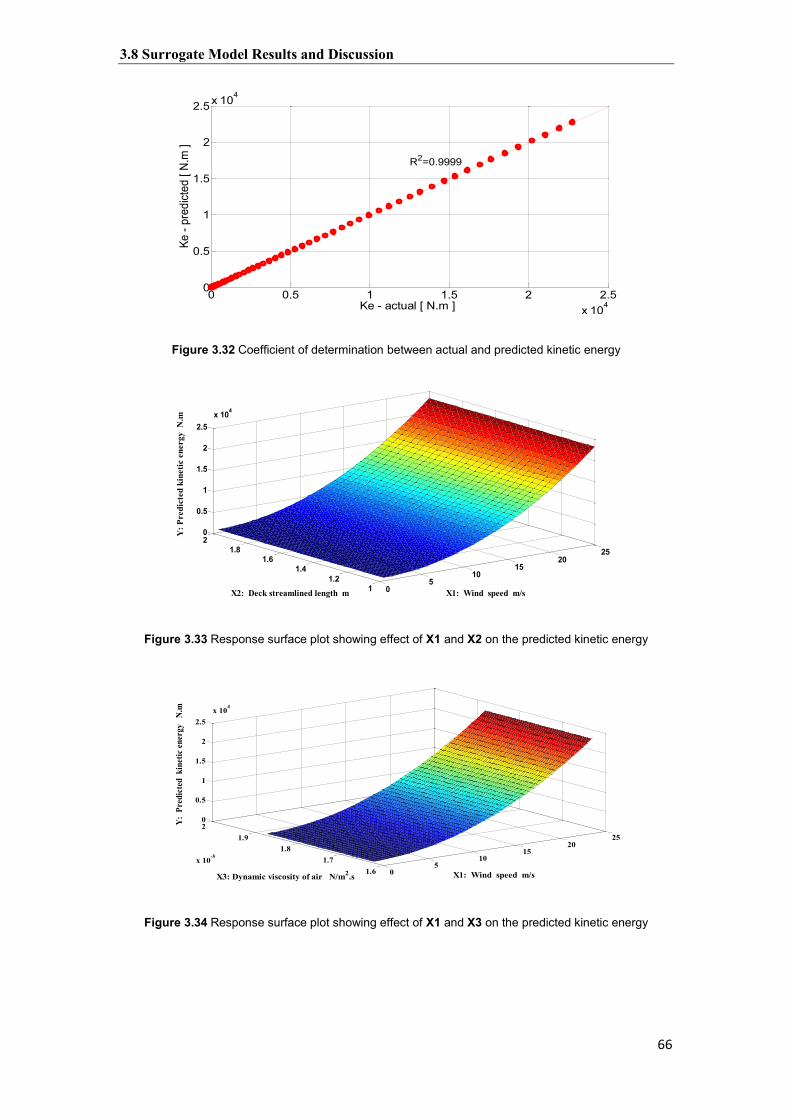
3.8 Surrogate Model Results and Discussion
66
Figure 3.32 Coefficient of determination between actual and predicted kinetic energy
Figure 3.33 Response surface plot showing effect of X1 and X2 on the predicted kinetic energy
Figure 3.34 Response surface plot showing effect of X1 and X3 on the predicted kinetic energy
0 0.5 1 1.5 2 2.5x 10⁴
0
0.5
1
1.5
2
2.5x 10⁴
Ke - actual [ N.m ]
Ke -
pred
icted
[ N.
m ]
R2=0.9999
05
1015
2025
11.2
1.41.6
1.820
0.5
1
1.5
2
2.5x 104
X1: Wind speed m/sX2: Deck streamlined length m
Y: P
redi
cted
kin
etic
ene
rgy
N.m
05
1015
2025
1.61.7
1.81.9
2
x 10-5
0
0.5
1
1.5
2
2.5x 104
X1: Wind speed m/sX3: Dynamic viscosity of air N/m2.s
Y: P
redi
cted
kin
etic
ener
gy
N.m

3.8 Surrogate Model Results and Discussion
67
Figure 3.35 Response surface plot showing effect of X2 and X3 on the predicted kinetic energy
Quadratic and interaction terms are used to build the surrogate model to calculate the lift
force generated in the deck. The coefficient of determination R2calculated between the actual
and the predicted lift force was R2 = 99.99 % which is a very good approximation for the
prediction of lift force where only 0.0 1% of the system response remains unexplained (see
Figure 3.36).
Figure 3.36 Coefficient of determination between actual and predicted lift force
The next response surface plots express on the relation between each two aerodynamic
parameters X1X2, X1X3, X2X3 and the predicted lift force generated in the deck as shown in
Figure 3.37, Figure 3.38 and Figure 3.39 which have been generated using MATLAB codes.
-500 0 500 1000 1500 2000 2500 3000-500
0
500
1000
1500
2000
2500
3000
Fl - actual [ N ]
Fl -
pred
icte
d [ N
]
R2=0.9999
11.2
1.41.6
1.82
1.61.7
1.81.9
2
x 10 -5
-60
-40
-20
0
20
X2: Deck streamlined length mX3: Dynamic viscosity of air N/m2.s
Y:
Pred
icte
d ki
netic
ene
rgy
N.m

3.8 Surrogate Model Results and Discussion
68
Figure 3.37 Response surface plot showing effect of X1 and X2 on the predicted lift force
Figure 3.38 Response surface plot showing effect of X1 and X3 on the predicted lift force
Figure 3.39 Response surface plot showing effect of X2 and X3 on the predicted lift force
05
1015
2025
11.2
1.41.6
1.82
-1.8
-1.6
-1.4
-1.2
-1
-0.8x 104
X1: Wind speed m/sX2: Deck streamlined length m
Y:
Pred
icte
d lif
t for
ce
N
05
1015
2025
1.61.7
1.81.9
2
x 10-5
-500
0
500
1000
1500
2000
2500
X1: Wind speed m/sX3: Dynamic viscosity of air N/m2.s
Y:
Pred
icte
d lif
t for
ce
N
11.2
1.41.6
1.82
1.61.7
1.81.9
2
x 10-5
-1000
-800
-600
-400
-200
0
200
X2: Deck streamlined length mX3: Dynamic viscosity of air N/m2.s
Y:
Pred
icte
d lif
t for
ce
N

3.9 Sensitivity Analysis Results and Discussion
69
3.9 Sensitivity Analysis Results and Discussion
The main orders of sensitivity indices for each aerodynamic parameter in addition to their
interaction orders were calculated considering the convergence results which recommended
using 250 samples to calculate the kinetic energy and 200 samples to calculate the lift force
for VIV of the deck (see Figure 3.40 and Figure 3.41). Supporting on the calculated results, the
total sensitivity indices for each aerodynamic parameter have been calculated (see Table 3.3).
In relation with the kinetic energy, the total order sensitivity index of aerodynamic parameter
(wind speed) is 0.9997, which is the biggest aerodynamic parameter, while the total order
sensitivity index of X2 is 0.0036. Furthermore, the total order sensitivity index of X3 is
0.0040, this means that the kinetic energy of the system is 99.97% due to variation in the
wind speed, and it is 0.36% due to the variation in the deck streamlined length. In the other
hand, it is 0.40% due to the variation in the dynamic viscosity of the wind. While the
interaction index between the aerodynamic parameters X1 and X2 is 0.0023 and between X1
and X3 is 0.0027, while between X2 and X3 is 0.0001, which means that there is a small
interaction between the aerodynamic parameters taking part in the variation of the kinetic
energy of the system due to vortex shedding.
While considering the lift force, the total order sensitivity index of X1 is 0.8375, which is the
biggest aerodynamic parameter, while the total order sensitivity index of X2 is 0.1707.
Furthermore, the total order sensitivity index of X3 is 0.0294, this means that the lift force is
dependable 83.75% on the wind speed variation, while it is 17.07% due to the deck
streamlined length variation, and it is 2.94% due to the variation in the dynamic viscosity of
the wind. While the interaction index between X1 and X2 is 0.0157 and between X1 and X3
is 0.0150, in the other hand, between X2 and X3 is 0.0012. This proofs that the surrogate
model is non-additive because there are small interactions between the aerodynamic
parameters especially between wind speed and deck streamlined length once and between
wind speed and dynamic viscosity of the wind in other side take part in the variation of the lift
force generated in the deck, while not appreciable interaction between the deck streamlined
length and the dynamic viscosity of the wind is seen to affect the lift force.
3.9.1 Convergence of The Results
The process of global sensitivity analysis supporting on Sobol's sensitivity indices requires
sufficient samples of experiments to identify the predicted effect of the aerodynamic
parameters on the VIV of the deck through two related outputs. The most efficient number of
samples is being identified through the convergence of the sum of first orders and total

3.9 Sensitivity Analysis Results and Discussion
71
sensitivity indices of the aerodynamic parameters. All the sensitivity indices (first orders,
interaction orders and total orders) for each aerodynamic parameter have been calculated
using m MATLAB codes. Two outputs have been considered in the process of converges, the
kinetic energy and the lift force. Figure 3.40 and Figure 3.41 show the relation between the
number of samples and the sum of first orders sensitivity indices, in the same time between
the number of samples and the sum of total sensitivity indices of the three aerodynamic
parameters.
Table 3.3
Sensitivity indices
Sensitivity indices Kinetic energy Lift force
first order X1
first order X2
first order X3
sum of first orders
interaction between X1 and X2
interaction between X1 and X3
interaction between X2 and X3
total order of X1
total order of X2
total order of X3
sum of total orders
0.9937
0.0001
0.0001
0.9989
0.0023
0.0027
0.0001
0.9997
0.0036
0.0040
1.0073
0.8039
0.1510
0.0104
0.9971
0.0157
0.0150
0.0012
0.8375
0.1707
0.0294
1.0376
Figure 3.40 Convergence of sensitivity indices – Kinetic energy
0 50 100 150 200 250 300 350 40099.5
100
100.5
101
101.5
102
102.5
103
Ns
S i
Sum of first orders sensitivity indicesSum of total orders sensitivity indices

3.9 Sensitivity Analysis Results and Discussion
71
Figure 3.41 Convergence of sensitivity indices – Lift force
For the case of kinetic energy (see Figure 3.40), the two curves of the sum of first orders and
total orders of sensitivity indices at the beginning are starting without stability for coinciding
to reach convergence, this situation continues till 250 samples. After this stage the two curves
are starting to converge at the 250 number of samples, where the two curves continue to
remain in a stable. In the same way, for the lift force (see Figure 3.41) the two curves are
reaching convergence at 200 samples, and the coinciding pattern continues in a stable
situation.
The convergence results of the two output cases predetermine utilizing 250 and 200 samples
of experiments to efficiently calculate the predicted rational effects of each aerodynamic
parameter on both the variation of the kinetic energy and lift force respectively.
0 50 100 150 200 250 300 350 40099
100
101
102
103
104
105
106
Ns
S i
Sum of first orders sensitivity indicesSum of total orders sensitivity indices

72

73
Chapter 4
Fluid-Structure Interaction and Lock-in Phenomenon
4.1 Vortex Induced Vibration (VIV) VIV can be known as the aerodynamic vibration which is caused by the alternate vortices
generated from the interaction between the object and wind flow. Normally, the
dimensionless constant called Strouhal number is used to evaluate the characteristic property
of each bluff-body in wind flow by means of the phenomenon called the vortex shedding
behind the object as shown in Equation (4.1) below.
( )
where the Strouhal number depends on body geometry and the Reynolds number , is
the across-wind dimension, is the mean velocity and is the primary frequency of the
vortex shedding. When the vortices shed in the wake region is exciting an elastically
supported body periodically, it will undergo a small response unless the Strouhal frequency
reaches close to the across- flow frequency of the structure. The surface pressure generates
in-line and across-flow forces with frequencies and simultaneously, where a pitching
moment has a frequency . Here, the body interacts with the flow strongly. This frequency
controls the vortex shedding even if the flow speed changes, which results in change of the
Strouhal frequency away by a few percent from the natural frequency, this phenomenon is
called lock-in [Dien, 1995; Kuroda, 1997; Larsen and Walther, 1997; Facchinetti et al., 2004;
Salvatori, 2007; Puckett et al., 2011; Bourguet et al., 2011; Tran, 2014]. It is known that the
across-wind force increases until limited cycle of oscillation amplitude reached during
synchronization. Also the along-structure correlation of force increases with oscillation
amplitude. The most qualified models of the mathematical modeling of lock-in phenomenon
are basing on coupled oscillators representing the structure and the wake [Diana et al., 2006].
Practically, the models of the single degree of freedom are usually considered in the structural
analysis, where a classical one is proposed by Simiu and Scanlan, 1996, through expressing
the across-wind force as: .

4.2 Fluid-Structure Interaction (FSI)
74
[ ( ) ( ) ( ) ( ( )
)
( )
] ( )
where , , , and are experimental parameters, functions of the Strouhal reduced
frequency = . In Equation (4.2), three terms are distinguished: harmonic forcing
term, a non-linear aerodynamic damping term, and an aerodynamic stiffness term. The
harmonic term represents the alternating lift where -in does not occur due to vortex-
shedding in the velocity ranges. The forcing term becomes negligible ( ≃ 0) in the region
close to lock-in, and the other terms are controlling the synchronized oscillations. Using Van
der Pol oscillator, the nonlinear damping term represents the self-limiting oscillations and the
stiffness term holds the frequencies synchronized in the lock-in region [Zhang, 2003 and
Salvatori, 2007].
Avoiding synchronization is suggested by Eurocode 1, but this phenomenon has been
observed where the wind speed can range between wide limits, especially because a wide
range of wind speeds result in the development of the phenomenon. Modifying the cross-
section geometry of the bridge deck changes the vortex shedding behavior as a result
changing the amplitude and the frequency of the oscillations but it does not development of
the phenomenon [Andersson and Ahl, 2011].
4.2 Fluid-Structure Interaction (FSI)
Multi-physics cases are very difficult to being solved using analytical methods. They mostly
should be solved by using numerical simulations or using experiments. The most advanced
techniques and the reputed commercial software in CFD and CSD have made the numerical
simulation possible. FSI within models created using finite element programs is mostly
conducted by the use of a node to surface contact algorithm. Standard FSI algorithm has three
steps, computing the surfaces and their normal, then conducting contact search between the
nodes of the fluid that might contact with the surface and the last is applying penalty forces to
the nodes of the fluid so that to prevent the fluid from penetrating the surfaces [Rabczuk et
al., 2010]. Exchange of the information is done at the interface between the two solvers, this
is called the coupling which is of two types, the first is the one-way coupling and the second
is the two-way coupling.
4.2.1 One-Way FSI In one-way coupling, the motion of the fluid flow influences the solid structure but the
reaction of the solid structure on the fluid flow is neglected. Also the two-way coupling can
be possible. The calculation of the fluid flow is performed until reaching convergence. The

4.2 Fluid-Structure Interaction (FSI)
75
resulted forces at the interface from the fluid calculation are being interpolated to the
structural mesh. Then the calculations of the structural dynamic are performed until meeting
convergence criterion. The process is repeated until reaching the end time. Interaction
between fluids and structures problems can be considered uncoupled problems within both
separate domains. In these problems assumption is formulated that a domain is driven by
another, but the driven domain has no feedback effect on the driving domain. CFD model
simulation provides the pressure on the structure by the fluid, and they are applied like load
condition or as a boundary for the finite element analysis simulation of the configuration,
where no feedback is done by the deflection into the CFD, which is called one-way fluid
structure interaction. Many civil structures are excited by dynamic wind loading which is an
example of one-way fluid structure interaction. In these cases, the structural motion and
displacement have no appreciable effect on the driving wind loads, where the structure can be
separately analyzed, or by treating the structure as uncoupled from the driving wind under
certain loads in the range of interest [Iliev et al., 2004; Van Zuijlen et al., 2006; Gale, 2008;
Hassler, 2009; Schmucker et al., 2010; Benra et al., 2011; Hansen, 2013].
4.2.2 Two-Way FSI In two-way coupling the motion of the fluid flow influences the solid structure and in the
same time the fluid flow is influenced by the reaction of the structural solid. During the
beginning of the time step, convergence solutions of the fluid calculation produce forces
acting on the solid structure. Next, the forces are interpolated to the structural mesh the same
as in the one-way coupling and the solutions from the structural solver is determined with the
fluid forces as boundary conditions. As a result the mesh is deformed according to the
response of the structure. The values of the displacements are interpolated to the fluid mesh
which results in deforming the fluid domain. The process is repeated until reaching the
convergence between the force and displacement values below the limit that was previously
determined [Onate and Garcia, 2001 and Raja, 2012]. When both the fluid and the structure
are interacting in a system of feedback in some practical applications in the engineering area,
the structural displacements generated by the fluid motion enhance the fluid forces, and this is
called two-way fluid structure interaction. In this case often the amplitude of the deflection of
the structure is large. The wind power plant is one example of this type of analysis [Van
Zuijlen et al., 2006; Forster, 2007; Razzaq et al., 2010; Benra et al., 2011; Liaghat, 2014].
In the general form, the FSI can be represented by the coupling both the equation of the
motion of the structure and the fluid. The equation of the motion of the structure can be
expressed as:

4.3 Finite Element Models
76
( )
where is the structural mass matrix, the structural damping matrix, the structural
stiffness matrix, the applied load vector, and the nodal displacement vector where the
dot denotes the time derivative. When the stagnant fluid is surrounding the oscillating
structure, the fluid effects on the structure should be accounted for. While the structure is
oscillating, the close fluid to the surface of the structure is starting to undergo motion in such
a way that the structure becomes affected by additional fluid force . As a result Equation
(4.3) represents the forced oscillation form, where is the fluid reaction on the structural
movement, and the decomposition of the force into three parts acting in-phase with the
displacement vector , the velocity vector and the acceleration vector of the structure is
possible [Bonisch et al., 2008; Von, 2012; Hengstler, 2013].
The accuracy of the two-way coupling is obvious, especially in large deflection cases where
the structural deformation influences the fluid field strongly. In strong two-way coupling,
solutions are of second order time accuracy, and they are more stable. In one-way coupling
conservation of energy at the interface is not guaranteed, but in two-way coupling is. There is
a benefit of one-way coupling simulations that ends with significant lower computational
time. The second benefit is that the fluid mesh has deformations without need to be
calculated, which result in producing a constant quality of the mesh. The effects of FSI for the
cases of totally or partially submerged body in a fluid flow with a free surface can't be
accurate predicted especially in cases related to civil engineering, offshore engineering and
naval architecture [Onate and Garcia, 2001 and Schmucker et al., 2010].
4.3 Finite Element Models The models of the segmental bridge deck are generated in ABAQUS once in CFD and
another in CSD. The CFD model is with a dimension 2.6 m height and total width of 22 m as
shown in Figure 4.1.a. The thickness is 0.01 m (should be very small so as to be treated as a
2D model). The flow domain size is 140 m length and 40 m height, the position of the deck
model in the flow domain should be in a position so that to facilitate a proper area to show the
vortex shedding in the downstream in addition to an appropriate area above and under the
deck model to show the boundary layers around the deck with the separation points (see
Figure 4.1.b). Material properties for the CFD model are assigned where the air density is
assigned 1.29 kg/m3 and the dynamic viscosity of the air is assigned 1.8E-05 Pa.s.

4.3 Finite Element Models
77
Figure 4.1.a Deck model dimensions
Figure 4.1.b Flow domain size
Figure 4.1.c The CSD model
The CFD model part is meshed using CFD element fluid family with FC3D8: A-8 node
linear fluid brick. The deck wall assigned with 0.4 element size and the flow domain with 1
element size. The CSD model has the following material properties: concrete density is
assigned 2643 kg/m3, Young’s modulus 200E+08 and the Poissons ratio 0.2 (see Figure 4.1.c).
The role of the steel reinforcement is neglected for simplicity because the thickness of the
CSD model is too small 0.01m and the reinforcement has no direct contact with the air. The
CSD model part is meshed using 3D stress family with C3D8R: A-8 node linear brick
reduced integration hourglass control.
A flow step with 100 seconds duration is created for the CFD model in addition to assigning
predefined Spalarat-Allmaras model turbulence due to very large number of Reynolds number
and or due to random oscillation of the time history curve of the kinetic energy dissipated, and

4.3 Finite Element Models
78
creating another dynamic implicit step with 100 seconds for the CSD model. The step time in
each model must be the same, in addition to adding interaction with the same name in each
model for the surfaces of interaction, also the important issue related to mesh generation is
equality of the mesh size in each model. The job is created for the simulation of CFD model
apart or one-way FSI approach, and another co-simulation job is generated for both the CFD
and the CSD models together or two-way FSI approach.
4.3.1 Boundary Conditions
Four boundary conditions are defined for the CFD and CSD models (Figure 4.2), fluid B.C
for the inflow and far fields assigning the air speed value in the horizontal direction only (zero
attack angle). The other two directions with zero magnitudes, fluid B.C for the outflow
assigning zero pressure and fluid B.C for the front and back of the flow model with zero
speed magnitude for the third direction perpendicular to the model (z-direction), and no-slip
fluid B.C for the wall condition of the deck.
Figure 4.2 Domains and fluid-structure interaction boundary conditions
A mesh size of 9943 elements would be utilized to mesh the CFD model. The mesh size of
the deck in the structural domain should be the same as the mesh size of it in the flow domain
at the interface so that to match or coincide. Depending on the desirable mesh size for the
CFD model, the related mesh size of the CSD model was 357 elements (without refinement
due to interface matching requirement (see Figure 4.3.a and Figure 4.3.b).

4.4 Results and Discussion
79
Figure 4.3.a CFD mesh size - 9943 elements
Figure 4.3.b CSD mesh size - 357 elements
4.4 Results and Discussion 4.4.1 Vortex Shedding Simulation
Generation of vortex shedding from the deck models exists with different patterns, and the
simulations are considered at the time 100 seconds. When considering one-way FSI approach
the vortex shedding for wind speed 1 m/s (see Figure 4.4) is generated and it is regular in
periodic shedding from the tail of the deck, but for two-way FSI approach and for the same
wind speed a simple vortex shedding exists with irregular shedding because the wind flow is
affected by the feedback of the deck which disturbs the periodic shedding style of the vortices
shed from the deck tail where the wind speed is not high (see Figure 4.5).

4.4 Results and Discussion
81
.
Figure 4.4 Vortex shedding one-way V=1 m/s Figure 4.5 Vortex shedding two-way V=1 m/s
For wind speed 10 m/s a very good and efficient regular vortex shedding style from the deck
exists for one-way FSI approach (see Figure4.6) but for two-way FSI approach and for the
same wind speed, the vortex shedding is generated with a different style which is an evidence
of effect of the deck feedback (CSD simulation) on the surrounding wind flow, where
increasing the wind speed increases the lift and drag forces as a result the disturbance in the
vortices will be detected (see Figure 4.7).
Figure 4.6 Vortex shedding one-way V=10 m/s Figure 4.7 Vortex shedding two-way V=10 m/s
While for wind speed 15 m/s another pattern of vortex shedding exists for one-way FSI
approach which is affected by increasing the wind speed where it changes the shedding style
and shape of the vortices (see Figure 4.8), but for two-way FSI approach and for the same
wind speed the vortex shedding is generated but without a vanishing pattern, this happens
because for higher wind velocities higher than the associated lock-in velocities leads to
vanishing of the vortex shedding for a range velocities because the amplitudes of vibrations of
the deck are increasing due to an increase in the lift and drag forces, hence the feedback of the
deck on the wind flow increases (see Figure 4.9) and it is possible that the lock-in
phenomenon and the vortex shedding generation restarts at higher wind velocities where this
needs a very long duration simulation process and computationally is much costly.
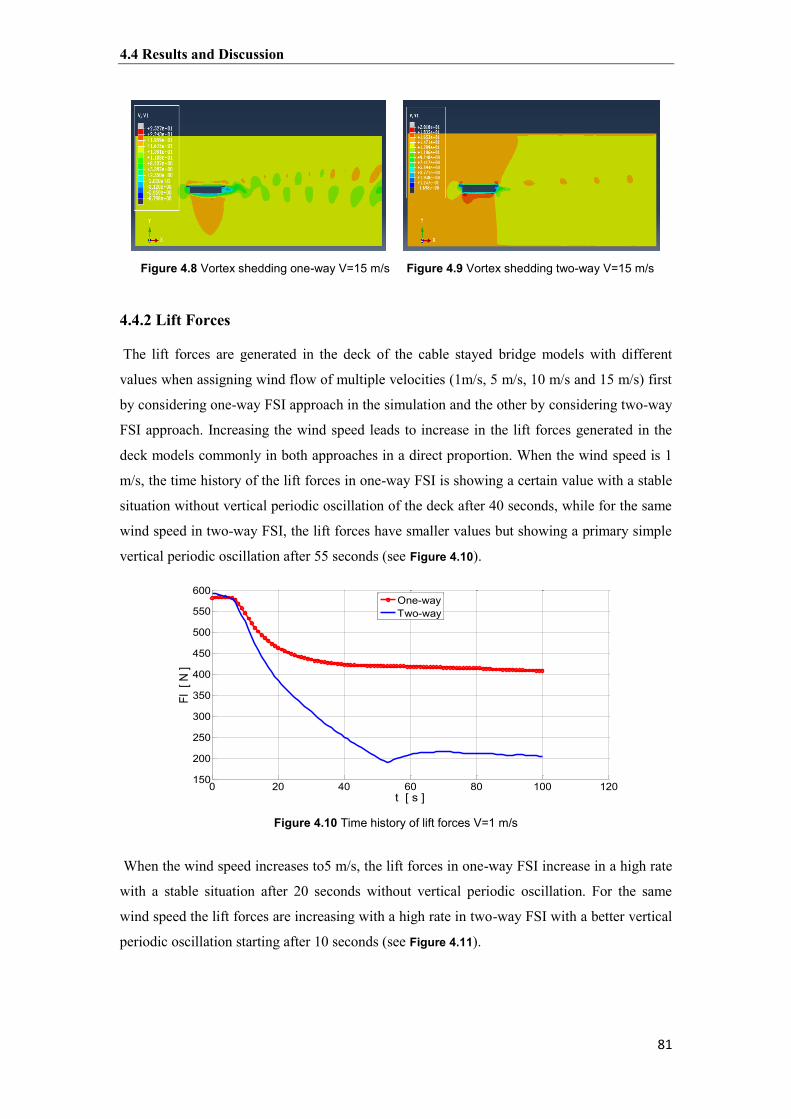
4.4 Results and Discussion
81
Figure 4.8 Vortex shedding one-way V=15 m/s Figure 4.9 Vortex shedding two-way V=15 m/s
4.4.2 Lift Forces The lift forces are generated in the deck of the cable stayed bridge models with different
values when assigning wind flow of multiple velocities (1m/s, 5 m/s, 10 m/s and 15 m/s) first
by considering one-way FSI approach in the simulation and the other by considering two-way
FSI approach. Increasing the wind speed leads to increase in the lift forces generated in the
deck models commonly in both approaches in a direct proportion. When the wind speed is 1
m/s, the time history of the lift forces in one-way FSI is showing a certain value with a stable
situation without vertical periodic oscillation of the deck after 40 seconds, while for the same
wind speed in two-way FSI, the lift forces have smaller values but showing a primary simple
vertical periodic oscillation after 55 seconds (see Figure 4.10).
Figure 4.10 Time history of lift forces V=1 m/s
When the wind speed increases to5 m/s, the lift forces in one-way FSI increase in a high rate
with a stable situation after 20 seconds without vertical periodic oscillation. For the same
wind speed the lift forces are increasing with a high rate in two-way FSI with a better vertical
periodic oscillation starting after 10 seconds (see Figure 4.11).
0 20 40 60 80 100 120150
200
250
300
350
400
450
500
550
600
t [ s ]
Fl [
N ]
One-wayTwo-way

4.4 Results and Discussion
82
Figure 4.11 Time history of lift forces V=5 m/s
Increasing the wind speed to 10 m/s, the lift forces in one-way FSI are increasing with a high
rate and the stability of the lift forces are obvious starting from 3 seconds without any vertical
periodic oscillation, while for the same wind speed the lift forces in two–way FSI are
increasing in a high rate too, but now the vertical periodic oscillatory behavior is much better
seen starting from 5 seconds (see Figure 4.12).
Figure 4.12 Time history of lift forces V=10 m/s
Now for the wind speed of 15 m/s, the lift forces for one-way FSI are increasing with a high
rate and show stability without showing vertical periodic oscillation after 2 seconds, but in
two-way FSI and for the same wind speed, the lift forces are increasing with a high rate
exhibiting significant vertical periodic oscillation with bigger frequency after 3 seconds (see
Figure 4.13).
0 20 40 60 80 100 1202000
4000
6000
8000
10000
12000
14000
16000
t [ s ]
Fl [
N ]
One-wayTwo-way
0 20 40 60 80 100 1201
2
3
4
5
6
7x 10⁴
t [ s ]
Fl [
N ]
One-wayTwo-way

4.4 Results and Discussion
83
Figure 4.13 Time history of lift forces V=15 m/s
The difference in the lift forces between one-way and two-way approaches is due to kinetic
energy dissipation in the latter approach which results in smaller values for lift forces. The
results of the lift forces in one-way FSI is an evidence that this approach is not sufficient in
detecting the actual VIV phenomenon, but the two-way FSI have a perfect ability in detecting
it. This means that the amplitudes of the lift displacement in the deck are predicted with lower
values of wind velocities, and thus the lock-in phenomenon is better predicted in earlier
stages.
4.4.3 Drag Forces For Drag forces, when one-way FSI approach is considered in the simulation process, the
drag forces increase in a direct proportion but the pattern of the horizontal periodic vibration
response of the deck models is not regular when the wind flow speed increases between (1
m/s to 15 m/s). When the wind speed value is 1 m/s, considering one-way FSI, the drag forces
have a certain value with a stable horizontal periodic vibration starting after 5 seconds, but for
two-way FSI and for the same wind speed, the drag forces have smaller values compared to
previous approach, and the horizontal periodic vibration have a semi stable situation starting
after 12 seconds and by time it is decreasing in a small rate (see Figure 4.14).
When the wind speed is increasing to 5 m/s, in one-way FSI, the drag forces are increasing in
a large rate with a stable situation of horizontal periodic vibration but with a larger frequency
for the amplitudes starting from the beginning of the wind excitation directly. While for two-
way FSI and for the same wind speed, the drag forces are increasing with a high rate but still
smaller than its values for the previous approach, in addition to creation of sudden changes in
the amplitudes of the horizontal periodic vibration coinciding with the start of changes of
vertical periodic vibrations after 45 seconds (see Figure 4.15), which means that the changes in
0 20 40 60 80 100 1202
4
6
8
10
12
14
16x 104
t [ s ]
Fl [
N ]
One-wayTwo-way

4.4 Results and Discussion
84
the frequency of the lift amplitudes leads to the change in the drag amplitudes in the same
time.
Figure 4.14 Time history of drag forces V=1 m/s
Figure 4.15 Time history of drag forces V=5 m/s
Increasing the wind speed to 10 m/s, in one-way FSI, the drag forces are increasing in a large
rate again with a stable situation of horizontal periodic vibration but with a smaller frequency
for the amplitudes starting from the beginning of the wind excitation directly too. While for
two-way FSI and for the same wind speed, the drag forces are increasing with a high rate but
still smaller than its values for the one-way FSI approach, furthermore a creation of sudden
changes in the amplitudes of the horizontal periodic vibration coinciding with the start of
changes of vertical periodic vibrations after 25, 55 and 85 seconds (see Figure 4.16) which
means that the changes in the frequency of the lift amplitudes leads to the change in the drag
amplitudes in the same time, where in this case three times are obvious.
0 20 40 60 80 100 12080
100
120
140
160
180
200
220
240
t [ s ]
Fd [
N ]
One-wayTwo-way
0 20 40 60 80 100 1201000
2000
3000
4000
5000
6000
7000
t [ s ]
Fd [
N ]
One-wayTwo-way

4.4 Results and Discussion
85
Figure 4.16 Time history of drag forces V=10 m/s
Continuous increase of wind speed to 15 m/s, and considering one-way FSI, the drag forces
are increasing in a large rate again with a stable situation of horizontal periodic vibration but
frequency for the amplitudes becomes bigger. While in two-way FSI and for the same wind
speed, the drag forces are increasing with a high rate but still smaller than its values in one-
way FSI approach, and it is worthy to mention that a creation of sudden changes in the
amplitudes of the horizontal periodic vibration are coinciding with the start of changes of
vertical periodic vibrations after 20, 40, 60, 80 and 100 seconds (see Figure 4.17) which means
that the changes in the frequency of the lift amplitudes leads to the change in the drag
amplitudes in the same time for five times along duration of 100 seconds of wind excitation.
Figure 4.17 Time history of drag forces V=15 m/s
The difference in the drag forces between one-way and two-way approaches is due to kinetic
energy dissipation in the latter approach which results in smaller values for drag forces. It is
obvious that the lift forces value in one-way FSI approach is three times the drag forces value
approximately for all the wind speed cases, compared to two-way FSI approach the lift forces
0 20 40 60 80 100 1200.5
1
1.5
2
2.5
3x 10⁴
t [ s ]
Fd [
N ]
One-wayTwo-way
0 20 40 60 80 100 1201.5
2
2.5
3
3.5
4
4.5
5
5.5
6x 10⁴
t [ s ]
Fd [
N ]
One-wayTwo-way

4.4 Results and Discussion
86
value is twice the drag forces value, the reason is the same which is related to the kinetic
energy dissipation.
4.4.4 Kinetic Energy The vibrational kinetic energy of the system is calculated from the simulation of vortex-
induced vibration of the deck models of a long span bridge due to a wind excitation in
ABAQUS for both the on-way and two-way FSI approaches. The results are for duration of
50 seconds. It is obvious that kinetic energy for the one-way approach is increasing from
4850 N.m to 4975 N.m and after this stage it becomes stable approximately till t = 20
seconds, while for the two-way approach this value is not stable in the beginning 20 sec with
a decreasing value from 4800 N.m and after that it becomes stable for the remain 30 seconds
with a value of 4525 N.m (see Figure 4.18). This means that the kinetic energy of the vibrating
system in one-way approach is still the same value approximately because the effect of the
structural model of the deck on the surrounding wind has not been considered and no
exchange of energy exists from the deck to the wind, so the overall kinetic energy remains
high and stable compared to that in two-way approach, but due to exchange of kinetic energy
between the deck and the wind together in two-way approach and large dissipation of the
kinetic energy in this process, the overall kinetic energy is less than of it in the on-way
approach.
Figure 4.18 Time history of the simulations kinetic energy
4.4.5 Lock-In Phenomenon At lock-in region, the vortex shedding is generated more efficiently. For one-way FSI
approach this phenomenon starts to appear clearly at wind speed of 11.5 m/s with regular
periodic and stable shape of the vortices shedding from the tail of the deck. The simulations
of the simulations are captured at the time histories 11.5 m/s, 11.7 m/s and 11.9 m/s. When
0 5 10 15 20 25 30 35 40 45 504500
4600
4700
4800
4900
5000
t [ s ]
KE [
N.m
]
One-wayTwo-way

4.4 Results and Discussion
87
the two-way FSI approach is considered, the vortex shedding generates with irregular style
due to the movement of the deck and its feedback on the surrounding wind flow for all wind
speed cases. The similarity in vortex shedding style with respect to the shape of the vortices
and the periodic pattern for all wind speed values for both the one-way and two-way
approaches is an indication of the lock-in phenomenon where the frequency of vortex
shedding remains constant approximately (see Figure 4.19).
One-way approach V=11.5 m/s Two-way approach V=11.5 m/s
One-way approach V=11.7 m/s Two-way approach V=11.7 m/s
One-way approach V=11.9 m/s Two-way approach V=11.9 m/s
Figure 4.19 Vortex shedding at Lock-in region

4.4 Results and Discussion
88
When only the one-way FSI approach is considered in the simulation, the lock-in
phenomenon exists at the wind speed of 11.5 m/s approximately but it is not quite regular and
the associated vortex shedding frequencies are near to 1.5 Hz till wind speed magnitude of 12
m/s, and after that range the vortex shedding frequency begins to increase in magnitude in a
linear proportion with the wind speed as shown in Figure 4.20.
Figure 4.20 Wind speed versus Vortex shedding frequency - Lock-In phenomenon
When considering the two-way FSI approach, the same phenomenon starts to appear at the
wind speed magnitude of 10 m/s and ends at 11.5 m/s in a regular path compared to the
previous approach, while the associated vortex shedding frequencies are 1.18 Hz. The vortex
shedding frequency after the lock-in region increases rapidly to 1.45 Hz and starts to
undertake a linear proportion approximately. This indicates that the FSI has an important and
effective role in detecting the actual region where the lock-in phenomenon starts to generate
and determines the associated shedding frequencies for lower natural frequencies of the
system.
4.4.6 Lift Coefficient The results of the relation between the Reynolds number and the lift coefficient Cl for the
deck model when the wind speed changes from 1 m/s to 15 m/s when considering one-way
FSI approach, the lift coefficient reaches a maximum value of 0.4 at Reynolds number value
of 0.75E+06, and the value of the lift coefficient is unstable until the Reynolds number
magnitude 0.9E+06, after that the relation becomes stable approximately for a lift coefficient
value -0.4 without appreciable changes in the value of the lift coefficient (see Figure 4.21).
0 5 10 150
0.5
1
1.5
2
U [ m/s ]
Ns
[ H
z ]
One-wayTwo-way

4.4 Results and Discussion
89
Figure 4.21 Reynolds number versus lift coefficient
The results of the relation between the Reynolds number and the lift coefficient when taking
in account the two-way FSI approach, show that the maximum value of the lift coefficient is -
0.3 begins from the Reynolds number value 0.9E+06 and in the same way as previous
approach it is unstable until the latter value of the Reynolds number and becomes stable after
that point.
4.4.7 Drag Coefficient The results of the relation between the Reynolds number and the drag coefficient Cd for
the deck model when the wind speed changes from 1 m/s to 15 m/s when considering one-
way FSI approach, the drag coefficient reaches a maximum value of 0.023 at Reynolds
number value of 1.5 E+06, and the value of the drag coefficient is stable at 0.02
approximately (see Figure 4.22).
Figure 4.22 Reynolds number versus drag coefficient
0 0.5 1 1.5 2 2.5x 10⁶
-1
-0.8
-0.6
-0.4
-0.2
0
0.2
0.4
Re [ ]
Cl [
]
One-wayTwo-way
0 0.5 1 1.5 2 2.5x 10⁶
-0.02
-0.01
0
0.01
0.02
0.03
0.04
Re [ ]
Cd
[ ]
One-wayTwo-way

4.4 Results and Discussion
91
While the relation between the Reynolds number and the drag coefficient when the two-way
FSI approach is used, show that the maximum value of the lift coefficient is 0.005 begins
from the Reynolds number value 4.0E+05 and it becomes stable starting from Reynolds
number value 0.8E+06 approximately.
4.4.8 Reynolds Number The Reynolds number calculations in each approach have been determined for multiple
wind velocities supporting on the results of the simulations in ABAQUS in addition to lift and
drag coefficients (see Table 4.1).
Table 4.1
Reynolds number versus lift and drag coefficients for multiple wind velocities
Wind
speed m/s Reynolds
number one-way
Reynolds number two-
way
Lift coefficient One-way
Lift coefficient two-way
Drag coefficient one-way
Drag coefficient two-way
1
2
3
4
5
6
8
10
12
15
1.50E+05
3.00E+05
4.50E+05
6.00E+05
7.51E+05
9.01E+05
1.20E+06
1.50E+06
1.80E+06
2.25E+06
1.50E+05
3.00E+05
4.50E+05
6.00E+05
7.51E+05
9.01E+05
1.20E+06
1.50E+06
1.80E+06
2.25E+06
0.3625
0.097
-0.267
-0.3405
0.398
-0.386
-0.3585
-0.4075
-0.362
-0.365
-0.77
-0.866
-0.445
-0.792
-0.419
-0.317
-0.311
-0.285
-0.269
-0.288
0.0212
0.01955
0.0213
0.0206
0.0216
0.0214
0.0206
0.02335
0.0208
0.0214
-0.0024
0.0042
0.0046
0.00285
0.00455
0.0045
0.0038
0.00325
0.00385
0.00405
4.4.9 Strouhal Number The calculations of the Strouhal number value for the deck models is between 0.322 and
0.324 for the one-way FSI approach, while for the two-way FSI approach this value is
between 0.285 and 0.308 (see Table 4.2). The relation between the Reynolds number and the
Strouhal number for the deck model when considering many cases of wind velocities for both
approaches is stable and linear approximately for one-way FSI approach but it is not stable
and nonlinear when adopting two-way FSI approach (see Figure 4.23).

4.4 Results and Discussion
91
This result proofs the fact that the Strouhal number is depending on the Reynolds number and
it is nearly with a value of 0.2 for a large range of Reynolds number, and the FSI concept is
better supporting this fact, this by comparing the results when considering two-way FSI
approach, where the Strouhal number is between (0.28-0.29) approximately until Reynolds
number value of (1E+06) but the Strouhal number value is constant at 0.32 until Reynolds
number value of 2.3E+06 when considering one-way FSI approach.
Table 4.2
Strouhal number versus vortex shedding frequency for multiple wind velocities
Figure 4.23 Reynolds number versus Strouhal number
Wind speed m/s
Shedding frequency one-way
Hz
Shedding frequency two-way
Hz
Strouhal number one-way
Strouhal number two-way
1
2
3
4
5
6
8
10
12
15
1.241E-01
2.490E-01
3.733E-01
4.962E-01
6.203E-01
7.472E-01
9.978E-01
1.248E+00
1.492E+00
1.865E+00
1.105E-01
2.208E-01
3.292E-01
4.549E-01
5.712E-01
6.758E-01
9.415E-01
1.154E+00
1.386E+00
1.777E+00
3.227E-01
3.237E-01
3.236E-01
3.225E-01
3.225E-01
3.238E-01
3.243E-01
3.244E-01
3.232E-01
3.233E-01
2.873E-01
2.870E-01
2.853E-01
2.957E-01
2.970E-01
2.928E-01
3.060E-01
3.000E-01
3.003E-01
3.080E-01
0 0.5 1 1.5 2 2.5x 10⁶
0.2
0.25
0.3
0.35
0.4
Re [ ]
St [
]
One-wayTwo-way

4.5 Validation of The FSI Models
92
4.5 Validation of The FSI Models
It is essential to accurately simulate the FE models and this depends on verification of the
numerical models through a comparison process against analytical solutions and or if it is
possible to compare it against experimental data. 4.5.1 Simiu and Scanlan Benchmark The results of the lock-in phenomenon determined from ABAQUS simulations in both one-
way FSI approach and two-way FSI approach are compared with the compiled numerical
results obtained by Simiu and Scanlan. The lock in phenomenon simulation using two-way
FSI approach is better represents the actual phenomenon this by validation with the results
obtained by Simiu and Scanlan (see Figure 4.24).
Figure 4.24 Wind speed versus vortex shedding frequency- Lock-in phenomenon validation Where the period of equal vortex shedding frequencies is greatly similar compared to the
region of equal vortex shedding frequencies in the one-way FSI approach, where the start of
the phenomenon in one-way approach is at wind speed 11.5 m/s till 12 m/s, but for two-way
approach is starting from wind speed of 10 m/s till 11.5 m/s. This is indicates the importance
of the two-way FSI approach in simulating the generation of lock-in phenomenon as a result
the vortex shedding induced vibration in the deck of the long span bridges can be determined
more efficiently and predicted for earlier and wider range of wind velocities in addition to
considering lower natural frequencies of the system which enhances the safety of the structure
against the VIV.
0 5 10 150
0.5
1
1.5
2
U [ m/s ]
Ns
[ H
z ]
Simiu and ScanlanTwo-wayOne-way

4.5 Validation of The FSI Models
93
4.5.2 Flat Plate Model (Munson and Co-authors) Benchmark Another validation parameter is the drag coefficient Cd for the deck model for different
Reynolds number values, where the main effective parameter is the wind speed changes from
1 m/s to 15 m/s. The benchmark of validation for Cd is the results of a flat plate model used
by Munson and co-authors. The Cd results obtained in the flat plate model show that this
value is unstable until Reynolds number of 7.5E+05 where Cd value is 0.08 and becomes
stable in the region between 0.002 and 0.085 approximately but the Cd value is 0.02 for one-
way FSI approach and it is 0.005 for two-way FSI approach, which means that there is a very
good approximation between the results specifically between the benchmark and the two-way
FSI approach (see Figure 4.25).
Figure 4.25 Reynolds number versus drag coefficient validation
0 0.5 1 1.5 2 2.5x 10⁶
-0.01
0
0.01
0.02
0.03
0.04
0.05
0.06
0.07
0.08
Re [ ]
Cd [
]
One-wayTwo-wayFlat Plate Theory

94

95
Chapter 5
Control Efficiency Optimization of Multiple Tuned Mass Dampers
5.1 Tuned Mass Damper (TMD)
The concept of TMD application dates back to the 1940s [Den Hartog, 1947]. This device is
a linear dynamic vibration absorber system, consists of a secondary mass suspended via a
viscous damper and a spring from a point on the main structure. It is tuned to a certain
structural frequency of the structure such as a bridge in order to, when excited, the damper
will resonate out of phase with the motion of the bridge, i.e., the TMD mass oscillates in the
opposite direction of the main structure. Nowadays, establishment of this system succeeded in
reducing wind-induced vibrations in many structural systems due to their particularity, where
they need less construction and maintenance cost, in addition to that their operation is easy
when used in the mechanical and civil engineering systems [Tang, 1997; Webster and
Vaicaitis, 2003; Thamasungkeeti, 2009; Fujino et al., 2010; Kumar, 2011: Miyata, 2003;
Mishra, 2011; Shetty et al., 2013; Wang et al., 2014]. These devices are most effective when
positioned at places of highest amplitudes. Therefore, considering this feature supplies the
opportunity for energy dissipation through the damper inertia force acting on the main
system. There are two main functions carried out by the TMD system, firstly it decreases the
resonant response of the main structure, and secondly, increases the overall damping of the
structure by the dashpot attached to, supplying additional source of energy dissipation. The
modal damping is affected by the mass ratio within low frequency ratio range, and this effect
almost finishes in high frequency ratio cases. The damping ratio has a great effect on the
response of cable stayed bridges, and it is emphasized that under a particular combination of
mass ratio, frequency ratio and the difference in the modal damping ratios, the effect of non-
classical damping is highly important [Chen and Kareem, 2003; Huang, 2006; Abdel Raheem
and Hayashikawa, 2008; Caruso et al., 2009; Samani, 2010; Huang, 2011; Guo, 2012; Huang
et al., 2012; Casalotti et al., 2013; Behrens et al., 2013; Tran, 2014; Wen et al., 2015].

5.2 Multiple Tuned Mass Dampers (MTMDs)
96
5.1.1 Energy Dissipation Mechanism
FSI between the exciting wind and the long span bridge generates aerodynamic instabilities.
As a result the bridge deck would be prone to vertical and torsional vibrations. The deck
motion is due to feeding energy into the bridge system by the the wind forces during one
cycle of oscillation. The energy is exchanged by the phase shift between the vertical and the
torsional vibrations and it counteracts the energy absorption by structural damping of the
bridge. When the structural damping of the bridge is sufficiently low which can't dissipate
these vibrations, the application of TMD becomes one of the solutions to suppress these
vibrations and boost the structural damping of the bridge system [Tsai and Lin, 1993; Lin et
al., 2000; Gua et al., 2002; Chen and Kareem, 2003; Chen and Cai, 2004]. The energy
dissipation mechanism starts when the bridge deck vibrates, with the presence of the TMD,
this device would be excited by the motion of the deck. When the mass of the damper moves
in a certain direction, as the movement of the deck would be toward the opposite direction,
hence the damping of the deck vibration is accomplished. The kinetic energy of the bridge
structure transfers into the TMD system where its viscous damper absorbs it. In order to attain
the most efficient energy absorbing rate, the natural period of the TMD is tuned to the natural
period of the bridge system. This is why it is called (Tuned Mass Dampers), so the strategy of
TMD application is attempting to dissipate the energy responsible of feeding the vibration.
The viscous damper of the TMD should be adjusted to optimum value so that to maximize
absorption of the energy [Zivanovic et al., 2005; Feldmann and Heinemeyer, 2007;
Andersson et al., 2013; Xing et al., 2014].
5.2 Multiple Tuned Mass Dampers (MTMDs)
The performance of TMD application in long span bridges is sensitive to the difference of
frequency ratios between the TMD and the bridge structure, even when optimally designed,
leads to serious performance deterioration this when the dynamic characteristics of the
structure are different from those used to accomplish its optimum design. This can be
overcome by the use of MTMDs. One of the important parameter for MTMDs is the mass
distribution to reduce effectively the dynamic response of a main system. When the mass
distribution is controlled along with other design parameters like damping ratio, frequency
range, number of dampers, the control of the main system response is achieved. To increase
the robustness of the vibration control system to various uncertainties in the structure, the use
of more than one TMD is an effective solution, where MTMDs have distributed natural
frequencies around the controlled mode of vibration [Lin et al., 1999; Patil, 2010; Samani,
2010; Bandivadekar and Jangid, 2012; Wang et al., 2014]. Adopting wide frequency band

5.3 Concept of TMD Using Two-Mass System
97
width makes it more robust and less sensitive to the change of the frequency ratio than using
TMD [Igusa and Xu, 1994], in addition they are suggested to mitigate the vertical and
torsional vibrations and to boost the aerodynamic stability of the long span bridges, which
permits to control of more than one mode of a multi degree of freedom (MDOF) structure by
tuning each TMD to the corresponding vibration mode of the main structure, or by tuning the
TMDs to frequencies close to a certain mode of the system. Though, in spite of their higher
effectiveness and robustness compared to single TMDs, the use of MTMDs encounters lack
capabilities of real time retuning, consequently their adaptation to frequency varying
excitation is very hard. The optimum TMD system for a certain structure is that one which
minimizes the expected vibrations amplitudes. Practically, the design of a TMD begins by
setting the value of the mass ratio, usually set within 1% to 10% [Warburton and Ayorinde,
1980]. The selection of this parameter value depends on the space availability to place the
TMDs. Despite the fact that use of high mass ratio values aid to further decrease the vibration
amplitudes, it may not be reasonable or economic because additional weight of the TMDs
necessitates strengthening other structural elements. As soon as the value of the mass ratio has
been elected, other design parameters such as frequency ratio and damping coefficients of the
viscous dampers of the TMDs require to be assigned [Chen and Xiang, 1998; Gua et al.,
2001; Lin and Cheng, 2001; Lee and Li, 2005; Karmakar et al., 2012; Estrad and Hong,
2015].
5.3 Concept of TMD Using Two-Mass System
The equation of motion for primary mass as shown in Figure 5.1 is:
( )
( )
( )
where is the mass of the damper and is the primary mass.
( )
( )
( )
where is the velocity, is the acceleration, is the damping ratio of the mass damper
is the natural frequency of the mass damper, , are the damping ratio, natural
frequency, damping coefficient and stiffeness of the primary mass respectively.

5.3 Concept of TMD Using Two-Mass System
98
Figure 5.1 TMD attached to the primary mass
The equation of motion for tuned mass is given by:
( )
The purpose of adding the mass damper is to control the vibration of the structure when it is
subjected to a particular excitation. The mass damper is having the parameters; the mass ,
stiffness , and damping coefficient . The damper is tuned to the fundamental frequency
of the structure such that:
( )
( )
The primary mass is subjected to the following periodic sinusoidal excitation
( )
then the response is given by
( ) ( )
( ) ( )
where and denote the displacement amplitude, response and phase shift of the primary
mass simultaneously, are displacement amplitude and response of the damper
respectively. The critical loading scenario is the resonant condition. The solution for this case
has the following form:

5.4 Equation of Motion
99
√
( ( ⁄ ) ⁄
⁄ ( )
( ) ( )
(
) ( )
( )
The above expression shows that the response of the tuned mass is 90º out of phase with the
response of the primary mass. This difference in phase produces the energy dissipation
contributed by the damper inertia:
(
) ( )
( )
To compare these two cases, we can express Equation (5.12) in terms of an equivalent
damping ratio:
(
* ( )
where
√
( ⁄
⁄ ) ⁄ ( )
Equation (5.19) shows the relative contribution of the damper parameters to the total
damping. Increasing the mass ratio magnifies the damping. However, since the added mass
also increases, so there is a practical limit on it.
5.4 Equation of Motion
Based on the classical method of flutter analysis and relating to the vertical bending and
torsion of a bridge, the frequencies of the TMDs are tuned to the neighborhood of the flutter
frequency so as to increase the critical flutter wind speed as shown in Figure 5.2.

5.4 Equation of Motion
111
Figure 5.2 Location of TMDs for suppressing a- Vertical vibration and b- Torsional vibration
The equation of motion of multi-degree of freedom structure TMDs which consists of
structure, TMD1 and TMD2 motion attached to hth and kth degree of freedom subjected to
wind load is given in Equation (5.20) besides Equation (5.21) presents the modal analysis
expressions.
( )
{
} [
] {
} ( )
where is a vector of absolute displacement of the main structure; and are absolute
displacement of TMD1 and TMD2 respectively; is a vector of generalized-coordinate
displacement of the main structure; and are generalized displacement of TMD1 and
TMD2 respectively; and is an nth natural mode shape of the main structure without
TMD, normalizing such that modal mass = 1.
Substitute Equation (5.21) into Equation (5.20) and pre-multiply with transpose of gives
the equation of motion in modal coordinates, as shown in in Equation (5.22).
( )
[ ]
( ) ( )

5.4 Equation of Motion
111
[
]
[
]
[
]
( )
[
]
[
]
[
]
( )
where , ( ) represent mass, damping coefficient and stiffness of TMD1
and TMD2 respectively.
To achieve the most efficient response suppression of the bridge deck, the optimal damping
ratio of TMD should be considered and to simplify the analysis, structural damping to be
neglected. The optimum damping ratio and optimum frequency ratio parameters of randomly
vibration can be calculated by Equation (5.28) and Equation (5.29) respectively [Warburton
and Ayorinde, 1980], where is ratio of TMD mass by structure mass Equation (5.26) and
frequency ratio parameter Equation (5.27).
( )
( )
√ ( )
( )( ) ( )
√
( ) ( )
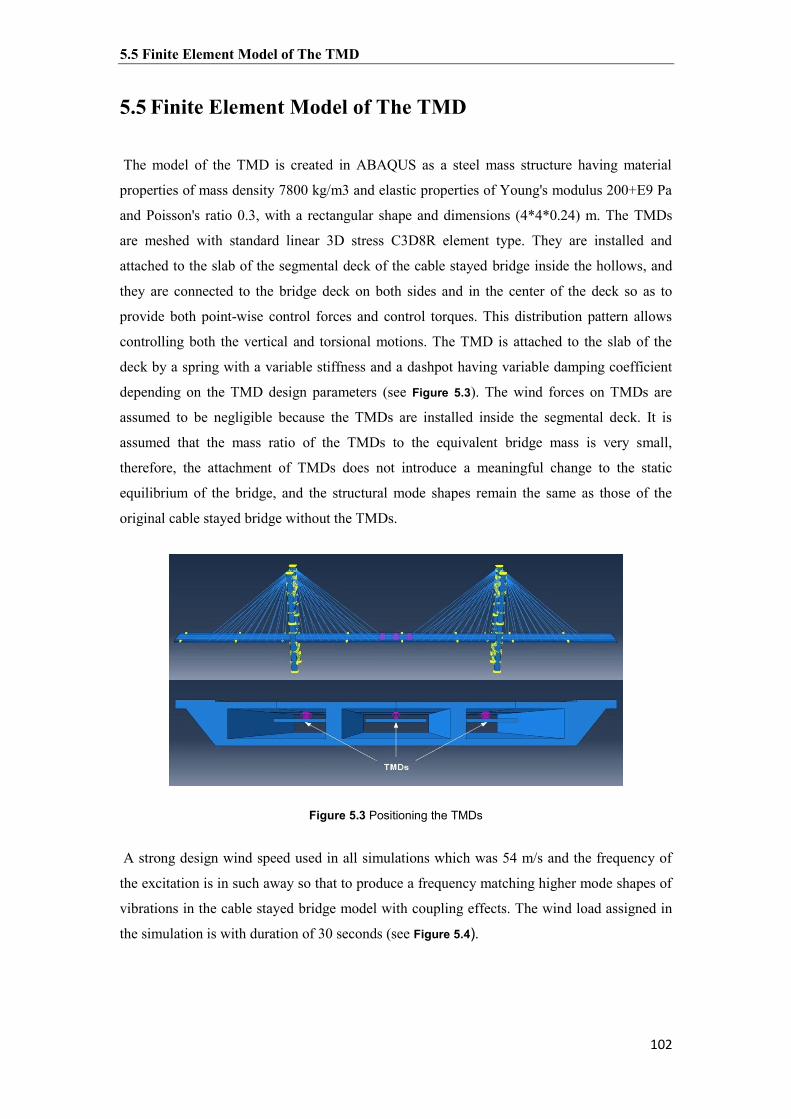
5.5 Finite Element Model of The TMD
112
5.5 Finite Element Model of The TMD
The model of the TMD is created in ABAQUS as a steel mass structure having material
properties of mass density 7800 kg/m3 and elastic properties of Young's modulus 200+E9 Pa
and Poisson's ratio 0.3, with a rectangular shape and dimensions (4*4*0.24) m. The TMDs
are meshed with standard linear 3D stress C3D8R element type. They are installed and
attached to the slab of the segmental deck of the cable stayed bridge inside the hollows, and
they are connected to the bridge deck on both sides and in the center of the deck so as to
provide both point-wise control forces and control torques. This distribution pattern allows
controlling both the vertical and torsional motions. The TMD is attached to the slab of the
deck by a spring with a variable stiffness and a dashpot having variable damping coefficient
depending on the TMD design parameters (see Figure 5.3). The wind forces on TMDs are
assumed to be negligible because the TMDs are installed inside the segmental deck. It is
assumed that the mass ratio of the TMDs to the equivalent bridge mass is very small,
therefore, the attachment of TMDs does not introduce a meaningful change to the static
equilibrium of the bridge, and the structural mode shapes remain the same as those of the
original cable stayed bridge without the TMDs.
Figure 5.3 Positioning the TMDs
A strong design wind speed used in all simulations which was 54 m/s and the frequency of
the excitation is in such away so that to produce a frequency matching higher mode shapes of
vibrations in the cable stayed bridge model with coupling effects. The wind load assigned in
the simulation is with duration of 30 seconds (see Figure 5.4).

5.5 Finite Element Model of The TMD
113
Figure 5.4 Wind speed fluctuation profile
The wind attack angle is 25° perpendicular to the longitudinal axis of the cable stayed bridge.
Frequency analysis has been undertaken to identify the first 20 mode shapes of vibrations for
the model. In this work we concentrate on the vertical and the torsional vibrations only. The
frequency magnitudes and the types of vibrations for eight mode shapes are available in Table
5.1.
Table 5.1
Vibration modes data
5.5.1 Mode Shapes Analysis
The process of designing the TMDs to control the vertical and torsional vibrations of the
deck in the cable stayed bridge needs to investigate the frequency analysis to identify the
0 5 10 15 20 25 30-4
-3
-2
-1
0
1
2
3
t [ s ]
Win
d sp
eed
fluct
uatio
n [ m
/s ]
Mode shape Type of vibration Frequency ( Hz )
1
3
6
7
9
11
16
20
Vertical
Vertical
Vertical –Torsional
Torsional
Vertical
Lateral –Torsional
Vertical –Torsional
Vertical –Torsional
0.242
0.509
0.776
0.789
0.883
0.986
1.208
1.631
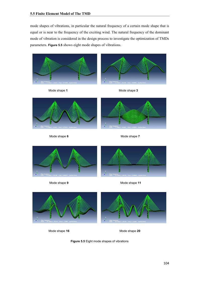
5.5 Finite Element Model of The TMD
114
mode shapes of vibrations, in particular the natural frequency of a certain mode shape that is
equal or is near to the frequency of the exciting wind. The natural frequency of the dominant
mode of vibration is considered in the design process to investigate the optimization of TMDs
parameters. Figure 5.5 shows eight mode shapes of vibrations.
Mode shape 1 Mode shape 3
Mode shape 6 Mode shape 7
Mode shape 9 Mode shape 11
Mode shape 16 Mode shape 20
Figure 5.5 Eight mode shapes of vibrations

5.5 Finite Element Model of The TMD
115
The vertical and torsional displacement time-histories at the mid span both for the center and
the outer edge are transformed into frequency domain signals using the Fast Fourier
Transform (FFT) technique by utilizing MATLAB codes, and the corresponding power
spectral density (PSD) of each time-history is shown in Figure 5.6. The energy of the vertical
vibrations of the bridge deck are concentrated on 0.7018 Hz, which is close to the sixth mode
vibration natural frequency of the cable stayed model; and the energy of the torsional
vibrations is centered on 0.7985 Hz, which is close to the seventh mode vibration natural
frequency. Results indicate that the vertical responses of the cable stayed bridge model are
dominated by the sixth mode, and the torsional responses are dominated by the seventh mode,
and it is clear that the two dominant modes are similar in their natural frequencies to a big
content. Thus, the sixth mode shape coupled (vertical-torsional) with natural frequency of
0.776 Hz would be the dominant vibration which would be based on to assign the TMDs
design data so that to get the optimum effect in suppressing the vertical and torsional
vibrations.
a- Vertical displacement
b- Torsional displacement
Figure 5.6 Power spectral densities of vertical and torsional displacements at the mid span
0 2 4 6 8 10 12 14 160
10
20
30
40
50
60
70
80
X: 0.7985Y: 74.69
Power spectral density PSD
Frequency f(Hz)
Powe
r P(m
2 .s)
0 2 4 6 8 10 12 14 160
10
20
30
40
50
60
X: 0.7018Y: 55.77
Power spectral density PSD
Frequency f(Hz)
Powe
r P(m
2 .s)

5.6 Optimization of TMD Parameters
116
5.6 Optimization of TMD Parameters TMD parameters are found using minimax optimization technique proposed by Tsai and Lin.
This technique to calculate the optimum values of frequency ratio and damping ratio for the
specified mass ratio is an iterative numerical search. For a fixed value of frequency ratio, the
maximum displacements for different values of damping ratios are found. Then the minimum
values are selected from the maximum displacements of response, which is the minimax
displacement for that value of frequency ratio. Then the above procedure is repeated for
different values of frequency ratio to find the minimax value of each frequency ratio. Finally,
the smallest minimizes are selected and corresponding frequency ratio and damping ratio are
the optimum parameters of the system having specified mass ratio. The numerical simulations
for all cases are implemented using ABAQUS finite element program.
5.6.1 Optimum Mass Ratio
When TMDs are designed, the mass ratio is an important parameter that is very sensitive to
design the overall weight and the number of these TMDs in order to get the most optimized
results for vibration mitigation. This parameter is the ratio of the TMDs total weight to the
total weight of the cable stayed bridge. Five mass ratios are considered which are (0.25 %,
0.75 %, 1.25 %, 1.75 % and 2.25 %). The dimensions of each TMD are designed (4*4*0.24)
m, they are distributed inside the three hollows of the segmental deck, and due to restriction
of place availability they are positioned parallel along the center line of the cable stayed
bridge model in a symmetrical pattern starting from the mid span region in the left and right
directions, so every mass ratio situation will take a certain number of TMDs (3 numbers, 9
numbers, 15 numbers, 21 numbers and 27 numbers) respectively for each mass ratio case.
Table 5.2 details the design data of the TMDs considering the mode shape 6 with natural
frequency of 0.776 Hz and constant frequency ratios of 1.0 and constant damping ratios of
0.05 which have been used in the simulations.
Table 5.2
Parameters of TMDs for multiple mass ratios
Mass ratio μ Frequency ratio f TMD stiffness Kd N/m
TMD damping coefficient Cd
N.s/m 0.25 % 1.0 54183 6982
0.75 % 1.0 162549 20947
1.25 % 1.0 270915 34912
1.75 % 1.0 379281 48876
2.25 % 1.0 487647 62841

5.6 Optimization of TMD Parameters
117
These situations are compared to the situation of the cable stayed bridge model excited by the
wind without the application of TMDs so that to compare the result to get the effect of mass
ratio on the vertical and torsional vibrations of the deck.
5.6.2 Results and Discussion
Considering the vertical vibration, the results confirm that the mass ratio of 2.25 % for
designing the TMDs is the optimum case to control the vertical vibration in this model. The
data is calculated for the point at the center above the deck at the mid span. Despite the fact
that the TMDs are in the beginning of the wind excitation are increasing the vertical vibration,
it needed approximately 10 seconds in order to start damping the vertical vibration
(buffeting). This case has an obvious effect in reducing the vertical vibration that reached
34.76 % of its magnitude without adding TMDs (see Figure 5.7). The case of minimum mass
ratio 0.25 % increased 33.20% of the vertical vibration, while the mass ratio of 0.75 %
reduced 12.77 % of the vertical vibration, and the mass ratio 1.25 % increased 9.24 % of the
vertical vibration. Finally the mass ratio 1.75 % has reduced the vertical vibration 15.12 % of
the vertical vibration (see Table 5.3).
Table 5.3
Vertical vibration control efficiency-Mass ratio
Figure 5.7 TMD mass ratio effect on the vertical vibration
Mass ratio μ Vertical vibration
control efficiency %
0.25 % -33.20
0.75 % 12.77
1.25 % -9.24
1.75 % 15.12
2.25 % 34.76
0 0.5 1 1.5 2 2.5-100
-50
0
50
100
u [ ]
Verti
cal v
ibra
tion
cont
rol e
ffici
ency
[ %
]

5.6 Optimization of TMD Parameters
118
This means that there is a nonlinear relation in the vertical vibration mitigation due to the
increase of TMDs mass ratio, and due to lack of place availability inside the segmental deck
and load effect in generating stresses due to the application of huge amounts of masses of the
TMDs, the mass ratio application should be limited to a desired quantity.
Relating to the torsional vibration of the deck, it was detected that the increase of the TMDs
mass ratio decreases the torsional (flutter) vibration to a significant amount as follows: for
mass ratio 0.25 % decreased 13.72 % and for mass ratio 0.75 % decreased 33.80 %, and for
mass ratio 1.25 % decreased 39.59 % while for mass ratio 1.75 % decreased 50.81% and
finally for mass ratio 2.25 % decreased 58.47 %, (see Figure 5.8 and Table 5.4). This is an
indication that the weight of the TMDs helps to balance the torsional vibration because the
TMDs are opposing the torsional vibration by their mass moments in the opposite direction.
This means that increasing mass ratio has a significant effect in mitigating the torsional
vibration of the deck.
Table 5.4
Torsional vibration control efficiency-Mass ratio
Figure 5.8 TMD mass ratio effect on torsional vibration
From the results above, it is clear the importance of using TMDs with the mass ratio 2.25%
to secure both the mitigation of the vertical vibration to 34.76% and the torsional vibration to
58.47%.
Mass ratio μ Torsional vibration
control efficiency %
0.25 % 13.72
0.75 % 33.80
1.25 % 39.59
1.75 % 50.81
2.25 % 58.47
0 0.5 1 1.5 2 2.50
20
40
60
80
100
u [ ]
Tors
iona
l vib
ratio
n co
ntro
l effi
cienc
y [ %
]

5.6 Optimization of TMD Parameters
119
5.6.3 Simulation of The Models
The mass ratio effect on the vertical and torsional vibrations of the cable stayed bridge is
simulated in ABAQUS and the following simulations (see Figure 5.9) show the situations of
vibrations due to wind excitation at time history of 30 seconds. The location of data collection
is at the mid span of the deck first at the center point and the second at the right and left outer
edges, where the first point is a reference to calculate the change in the vertical displacement
in each case and the second two points are used to calculate the change in the torsional
displacement.
No TMDs Mass ratio = 0.25 %
Mass ratio = 0.75 % Mass ratio = 1.25 %
Mass ratio = 1.75 % Mass ratio = 2.25 %
Figure 5.9 TMDs mass ratio effect on vertical and torsional vibrations
5.6.4 Optimum Frequency Ratio
Another parameter of designing TMDs is the frequency ratio, which is the ratio of the TMD
frequency and the natural frequency of the structure. The frequencies of the TMDs are tuned
to the natural frequency of the cable stayed bridge or near this frequency that belongs to the

5.6 Optimization of TMD Parameters
111
dominant mode shape of vibration. As mentioned in previous section, the dominant mode of
vibration is the mode shape 6, so the frequencies of the TMDs are tuned to 0.776 Hz which
has been calculated from the frequency analysis. Five frequency ratios cases which are (0.8,
0.9, 1.0, 1.1 and 1.2) would be utilized to detect the optimum reduction of the vertical and
torsional vibrations. Table 5.5 shows the magnitudes of the stiffness and the damping
coefficient of the TMDs for constant damping ratios of 0.05 and constant mass ratios of 2.25
% which was the best case to reduce the vertical and torsional vibrations.
Table 5.5
Parameters of the TMD for multiple frequency ratios
Frequency ratio f
Mass ratio μ
TMD stiffness Kd N/m
TMD damping coefficient Cd N.s/m
0.8 2.25 % 312094 50273
0.9 2.25 % 394994 56557
1.0 2.25 % 487647 62841
1.1 2.25 % 590052 69125
1.2 2.25 % 702211 75409
5.6.5 Results and Discussion
To consider the vertical vibration, the TMDs in the beginning of the wind excitation are
increasing the vertical vibration, and it needed approximately 10 seconds in order to start
mitigating the vertical vibration. It was detected that the case of frequency ratio 1.2 has the
largest effect in reducing the vertical vibration that reached 50.47% of its magnitude without
applying TMDs (see Figure 5.10). The case of frequency ratio 0.8 increased 21.76% of the
vertical vibration, while the frequency ratio of 0.9 decreased 6.16 % of the vertical vibration
and the frequency ratio of 1.0 decreased 34.76 % of the vertical vibration, but in other hand
the frequency ratio of 1.1 has decreased 46.18 % of the vertical vibration (see Table 5.6).
There is linearity in the vertical vibration mitigation due to the change in frequency ratio
design parameter till frequency ratio 1.0, after that the mitigation is less and tend to be stable
or with a very small change. The reduction in the vertical vibration between the two
frequency ratios 1.2 and 1.1 are near to each other, so the frequency ratio 1.1 can be
considered the suitable ratio to assign the TMDs frequencies which is near to the natural
frequency of the cable stayed bridge to optimize mitigating the vertical vibration of the deck.

5.6 Optimization of TMD Parameters
111
Table 5.6
Vertical vibration control efficiency-Frequency ratio
Figure 5.10 TMD frequency ratio effect on the vertical vibration
Related to torsional vibration, all the frequency ratio cases have shown significant reduction
of the torsional vibration of the deck (see Figure 5.11 and Table 5.7). The change in the ratios
has a very little effect on the results. Considering the frequency ratio 0.8, the torsional
vibration was reduced to 58.74 % and for frequency ratio 0.9 decreased 58.25%, and for
frequency ratio 1.0 decreased 58.47% while for frequency ratio 1.1 was decreased to 58.36 %
and finally for frequency ratio 1.2 decreased 58.12%. This means that changing the
frequency ratio of the TMDs has an appreciable effect in mitigating the torsional vibration of
the deck in the cable stayed bridge till reaching the frequency ratio 1.0 or near the natural
frequency of the cable stayed bridge but after that it has a small effect especially for large
TMD mass ratios.
From the results discussed above, it is essential to use the frequency ratio 1.1 to tune the
TMDs near to the natural frequency of the cable stayed bridge for the dominant mode shape 6
so that to control the vertical vibration to 46.18 % and to reduce the torsional vibration to
58.36%.
Frequency ratio f
Vertical vibration
control efficiency %
0.8 -21.76
0.9 6.16
1.0 34.76
1.1 46.18
1.2 50.47
0.75 0.8 0.85 0.9 0.95 1 1.05 1.1 1.15 1.2 1.25-80
-60
-40
-20
0
20
40
60
80
100
f [ ]
Verti
cal v
ibra
tion
cont
rol e
ffici
ency
[ %
]

5.6 Optimization of TMD Parameters
112
Table 5.7
Torsional vibration control efficiency-Frequency ratio
Figure 5.11 TMD frequency ratio effect on torsional vibration
5.6.6 Optimum Damping Ratio
The damping ratio parameter is considered for designing TMDs in vibration control, and it is
the ratio of the TMD damping coefficient to the critical damping coefficient of the main
structure. Five damping ratios (0.01, 0.05, 0.1, 0.15 and 0.2) are used to calculate the
optimum reduction in the vertical and torsional vibrations. Table 5.8 shows the magnitudes of
the stiffness and the damping coefficient of the TMDs considering these five damping ratio
cases with constant frequency ratios of 1.0 and constant mass ratios of 2.25 %.
Table 5.8
Parameters of the TMD for multiple damping ratios
Damping ratio
Mass ratio μ
TMD stiffness Kd N/m
TMD damping coefficient Cd
N.s/m 0.01 2.25 % 487647 12568
0.05 2.25 % 487647 62841
0.10 2.25 % 487647 125682
0.15 2.25 % 487647 188523
0.2 2.25 % 487647 251364
Frequency ratio f
Torsional vibration
control efficiency % 0.8 58.74
0.9 58.25
1.0 58.47
1.1 58.36
1.2 58.12
0.75 0.8 0.85 0.9 0.95 1 1.05 1.1 1.15 1.2 1.2550
55
60
65
70
f [ ]
Tors
iona
l vib
ratio
n co
ntro
l effi
cien
cy [
% ]

5.6 Optimization of TMD Parameters
113
5.6.7 Results and Discussion
Considering the vertical vibration, the results confirm that the damping ratio of 0.2 for
designing the TMDs is the optimum case to control the vertical vibration in this model. The
case of damping ratio 0.2 has the largest effect in reducing the vertical vibration which
reached 46.00% of its magnitude without applying TMDs (see Figure 5.12 and Table 5.9). The
case of damping ratio 0.01 decreased 33.03 % of the vertical vibration, while the damping
ratio of 0.05 decreased 34.76 % of the vertical vibration and the damping ratio of 0.1
decreased 38.93 % of the vertical vibration, but the damping ratio of 0.15 has decreased 43.74
% of the vertical vibration. Approximately a linear relation is apparent in the vertical
vibration mitigation due to the change of damping ratio.
Table 5.9
Vertical vibration control efficiency-Damping ratio
Figure 5.12 TMD damping ratio effect on the vertical vibration
Considering the reduction of the torsional vibration of the deck (see Figure 5.13 and Table
5.10). For damping ratio 0.01 the torsional vibration was reduced to 41.52% and for damping
ratio 0.05 decreased 41.54%, and for damping ratio 0.1 decreased 41.52 % , and for damping
ratio 0.15 was increased to 41.53 % and finally for damping ratio 0.2 decreased 41.56 %.
Damping ratio
Vertical vibration
control efficiency %
0.01 33.03
0.05 34.76
0.10 38.93
0.15 43.74
0.2 46.00
0 0.02 0.04 0.06 0.08 0.1 0.12 0.14 0.16 0.18 0.220
25
30
35
40
45
50
55
60
d [ ]
Verti
cal v
ibra
tion
cont
rol e
fficie
ncy
[ % ]

5.7 Validation of The TMDs Models
114
This means that changing the damping ratio of the TMDs has no effect on mitigating the
torsional vibration of the deck in the cable stayed bridge for this range of damping ratios.
Table 5.10
Torsional vibration control efficiency-Damping ratio
Figure 5.13 TMD damping ratio effect on the torsional vibration
Through the evaluation of the results, it is recommended to use the damping ratio 0.2 for
assigning TMDs damping coefficient so that to control the vertical vibration to 46.00% and to
reduce the torsional vibration to 41.56%.
From the minimax optimization technique results done for the three design parameters, it was
found that the use of TMDs with mass ratio 2.25%, frequency ratio of 1.1 and damping ratio
0.2 is the optimal case to guarantee the most efficient control of vertical and torsional
vibrations of the deck.
5.7 Validation of The TMDs Models The validation of the results for the TMDs design parameters is based on the comparison
with the benchmarks from the literature which have been considered in the introduction
section of this chapter. The first benchmark is the results obtained by Wang and co-authors
Damping ratio
Torsional vibration
control efficiency %
0.01 41.52
0.05 41.54
0.10 41.52
0.15 41.53
0.2 41.56
0 0.02 0.04 0.06 0.08 0.1 0.12 0.14 0.16 0.18 0.220
25
30
35
40
45
50
55
60
d [ ]
Tors
iona
l vib
ratio
n co
ntro
l effi
cienc
y [ %
]

5.7 Validation of The TMDs Models
115
for two TMDs design parameters mass ratio and damping ratio effects on the vertical
vibration of the deck for Sutong Bridge. The second benchmark is the results obtained by Lin
and co-authors for TMDs mass ratio effect on the vertical and torsional vibrations of the deck.
5.7.1 Wang and Co-authors Benchmark
The following Figure 5.14 is showing the curves of the results of the vertical vibration control
efficiency considering mass ratio obtained by Wang and co-authors and the results obtained
from the finite element model.
Figure 5.14 Validation for TMDs mass ratio effect on the vertical vibration of the deck
The control efficiency of the vertical vibration obtained from the results of Wang and co-
authors starts from 19.25% for mass ratio of 0.25% while it starts from -33.20% for the results
obtained from the finite element model. The curve of results for the FE model reaches near
the curve of the results of Wang and co-authors at mass ratio 0.75% with a control efficiency
of 12.73% and 25% for the latter. The nearest position is at mass ratio 2% with a value of
25% and 29% for the latter. The results obtained from the FE model showed a good
agreement with the results of Wang and co-authors at mass ratio range of (2% - 2.25%).
The curves of the results for the vertical vibration control efficiency considering the effect of
damping ratio for both Wang and co-authors and the finite element model are shown in Figure
5.15. The control efficiency of the vertical vibration obtained by Wang and co-authors start
with 26.70% for damping ratio of 0.01, while this output starts with 33.03% for the same
damping ratio obtained from the finite element model and the two response curves are
coinciding till the damping ratio 0.03. The control efficiency curve for Wang and co-authors
ends with 22.25% for damping ratio 0.08 and the curve of the finite element model has a
0 0.5 1 1.5 2 2.5-100
-50
0
50
100
u [ ]
Verti
cal v
ibra
tion
cont
rol e
ffici
ency
[ %
]
FE modelWang

5.8 Global Sensitivity Analysis
116
value of 36% at the same damping ratio. Supporting on the comparison between the two
results, a good agreement exists between them in the damping ratio range (0.01-0.03).
Figure 5.15 Validation for TMDs damping ratio effect on the vertical vibration of the deck
5.7.2 Lin and Co-authors Benchmark
Considering the aerodynamic coupling between the vertical and torsional vibrations for the
dominant mode shape of vibration, and when the mass ratio of the TMDs is 2%, the control
efficiency of the vertical vibration of the deck obtained from the results of the finite element
model was 25%, and it was the same value 25% obtained from Lin and co-authors. This
indicates that the two results have an excellent agreement, which pours to the validity of the
obtained results from the finite element model.
5.8 Global Sensitivity Analysis
Global sensitivity analysis studies how the uncertainty in the output of a model numerical or
otherwise can be apportioned to different sources of uncertainty in the model input. A good
sensitivity analysis should run analyses over the full range of plausible values of key
parameters and their interactions, to assess how impacts change in response to changes in key
parameters. Global sensitivity analysis methods such as Sobol's sensitivity indices have been
widely applied recently. Global sensitivity analysis explores the parameter space so that they
provide robust sensitivity measures in the presence of nonlinearity and interactions among the
parameters. Global sensitivity analysis, however, can be computationally intensive, since they
require sampling parameter sets. Several approximation methods have been developed to
0 0.01 0.02 0.03 0.04 0.05 0.06 0.07 0.08 0.09 0.10
20
40
60
80
100
d [ ]
Verti
cal v
ibra
tion
cont
rol e
ffici
ency
[ %
]
FE modelWang

5.9 Box-Behnken Sampling Method
117
reduce the computational cost. Global sensitivity analysis can provide additional information
for improving the system understanding.
Sobol sensitivity indices for the three design parameters (mass ratio, frequency ratio and
damping ratio) are utilized to obtain the control efficiency of vertical and torsional vibrations
of the deck after application of MTMDs.
5.9 Box-Behnken Sampling Method
Box-Behnken experimental design was based on to identify the relationship between the
response functions (vertical vibration and torsional vibration) of the deck in the cable stayed
bridge model and the three design variables of the TMDs (mass ratio, frequency ratio and
damping ratio). Box-Behnken design is rotatable second-order designs based on three-level
incomplete factorial designs. The special arrangement of the Box-Behnken design levels
allows the number of design points to increase at the same rate as the number of polynomial
coefficients. For three factors, for example, the design can be constructed as three blocks of
four experiments consisting of a full two-factor factorial design with the level of the third
factor set at zero.
Box-Behnken design requires an experiment number according to:
( )
where is the factor number and is the replicate number of the central point. Box-
Behnken is a spherical, revolving design. Viewed as a cube (Figure 5.16.a), it consists of a
central point and the middle points of the edges. However, it can also be viewed as consisting
of three interlocking factorial design and a central point (Figure 5.16.b). It has been applied
for optimization of several chemical and physical processes.
a- The design, as derived from a cube b- Interlocking factorial experiments
Figure 5.16 Box-Behnken experimental design

5.9 Box-Behnken Sampling Method
118
For the three-level three-factorial Box-Behnken experimental design, a total of 15
experimental runs shown in Table 5.11 are needed. The model is of the following form:
( )
where is the predicted response, model constant; , and independent variables;
, and are linear coefficients; , and are cross product coefficients and ,
and are the quadratic coefficients. The coefficients, i.e. the main effect and two
factors interactions have been estimated from the experimental results by computer
simulation programming applying least square method using MATLAB [Ferreira et al., 2004;
Rana et al., 2004; Kannan et al., 2004; Kincl et al., 2005; Souza et al., 2005; Ferreira et al.,
2007; Zhao and Tiede, 2011; Tekindal et al., 2012; Karmakar et al., 2012; Pasma et al., 2013;
Qiu et al., 2014].
Table 5.11
The level of variables chosen for the Box-Behnken design
Variable Symbol
Coded variable level
Low Center High
-1 0 +1
Mass ratio 0.0025 0.0125 0.0225
Frequency ratio 0.8 1.0 1.2
Damping ratio 0.01 0.105 0.20
The following Table 5.12 is showing both the coded and actual variable values that are related
to the 15 runs of the simulation of wind excitation with application of TMDs to reduce the
vertical and torsional responses of the deck utilizing variation in the three design parameters
mentioned above.

5.9 Box-Behnken Sampling Method
119
Table 5.12
Box-Behnken design with coded and actual values for three size fractions
Run no. Coded level of variables Actual level of variables
Mass ratio
Frequency ratio
Damping ratio
1 -1 -1 0 0.0025 0.8 0.105
2 +1 -1 0 0.0225 0.8 0.105
3 -1 +1 0 0.0025 1.2 0.105
4 +1 +1 0 0.0225 1.2 0.105
5 -1 0 -1 0.0025 1.0 0.01
6 +1 0 -1 0.0225 1.0 0.01
7 -1 0 +1 0.0025 1.0 0.2
8 +1 0 +1 0.0225 1.0 0.2
9 0 -1 -1 0.0125 0.8 0.01
10 0 +1 -1 0.0125 1.2 0.01
11 0 -1 +1 0.0125 0.8 0.2
12 0 +1 +1 0.0125 1.2 0.2
13 0 0 0 0.0125 1.0 0.105
14 0 0 0 0.0125 1.0 0.105
15 0 0 0 0.0125 1.0 0.105
5.9.1 Surrogate Models Results
The regression coefficients calculated from the second-degree model both for vertical and
torsional actual responses obtained using Box-Behnken method. Total of 15 runs are used to
formulate the surrogate models for the predicted vertical and torsional vibrations control
efficiency based on quadratic orders. The surrogate model for the case of vertical vibration
control efficiency has a coefficient of determination R2 of 99.45% (see Figure 5.17) which is a
very good representation of the predicted system response and just 0.55% of the system
response still unexplained.
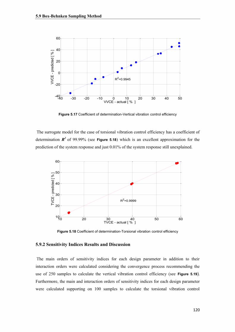
5.9 Box-Behnken Sampling Method
121
Figure 5.17 Coefficient of determination-Vertical vibration control efficiency
The surrogate model for the case of torsional vibration control efficiency has a coefficient of
determination R2 of 99.99% (see Figure 5.18) which is an excellent approximation for the
prediction of the system response and just 0.01% of the system response still unexplained.
Figure 5.18 Coefficient of determination-Torsional vibration control efficiency
5.9.2 Sensitivity Indices Results and Discussion
The main orders of sensitivity indices for each design parameter in addition to their
interaction orders were calculated considering the convergence process recommending the
use of 250 samples to calculate the vertical vibration control efficiency (see Figure 5.19).
Furthermore, the main and interaction orders of sensitivity indices for each design parameter
were calculated supporting on 100 samples to calculate the torsional vibration control
-40 -30 -20 -10 0 10 20 30 40 50-40
-20
0
20
40
60
VVCE - actual [ % ]
VVC
E - p
redi
cted
[ %
]
R2=0.9945
10 20 30 40 50 6010
20
30
40
50
60
TVCE - actual [ % ]
TVCE
- pr
edict
ed [
% ]
R2=0.9999

5.9 Box-Behnken Sampling Method
121
efficiency (see Figure 5.20). Supporting on the calculated results, the total sensitivity indices
for each design parameter have been calculated (see Table 5.13).
In relation with the vertical vibration control efficiency , the total order sensitivity index of
design parameter mass ratio X1 is 0.6979, this value is bigger than the total order sensitivity
index of design parameter frequency ratio X2 which is 0.2279, also it is much bigger than the
total order sensitivity index of design parameter damping ratio X3 which is 0.0883, this
means that the vertical vibration control efficiency is 69.79% due to variation in mass ratio
between the TMDs and the cable stayed bridge, and it is 22.79% due to the variation in
frequency ratio between the natural frequencies of the TMDs and the cable stayed bridge, also
it is 8.83% due to the variation in the damping ratio between them. While the interaction
index between the design parameter X1 and X2 is 0.0091 and between X1 and X3 is 0.0030,
while between X2 and X3 is 0.006, which means that there is a small interaction between the
input factors taking part in the variation of the vertical vibration control efficiency.
Table 5.13
Sensitivity indices
Sensitivity indices Vertical vibration control efficiency
Torsional vibration control efficiency
first order X1 0.6851 0.9997
first order X2 0.2176 0.0000
first order X3 0.0840 0.0001
sum of first orders 0.999329 0.999961
interaction between X1 and X2 0.0091 0.0001
interaction between X1 and X3 0.0030 0.0001
interaction between X2and X3 0.0006 0.0000
total order of X1 0.6979 0.9999
total order of X2 0.2279 0.0002
total order of X3 0.0883 0.0002
sum of total orders 1.0141 1.0003
While considering the torsional vibration control efficiency, the total order sensitivity index
of X1 is 0.9999, which can be named the controlling design parameter which is much bigger
than the total order sensitivity index of X2 which is 0.0002, also it is much bigger than the
total order sensitivity index of X3 which is 0.0002, this means that the torsional vibration
control efficiency is dependable 99.99% on the mass ratio variation, while it is 0.02% due to
the frequency ratio variation, and it is 0.02% due to the variation in damping ratio. While the
interaction index between X1 and X2 is 0.0001 and between X1 and X3 is 0.0001, while
between X2 and X3 is 0.0000, this proofs that the surrogate model is additive approximately

5.9 Box-Behnken Sampling Method
122
which means that there is no interaction between design parameters take part in the variation
of the torsional vibration control efficiency.
5.9.3 Convergence of The Results
The process of global sensitivity analysis supporting on Sobol's sensitivity indices requires
certain or adequate samples of experiments to find out the predicted effect of the design
parameters on the response of the system. The most efficient number of samples is being
identified through the convergence of the sum of first orders and total sensitivity indices of
the design parameters. All the sensitivity indices (first orders, interaction orders and total
orders) for each design parameter have been calculated using m MATLAB codes. Two
outputs have been utilized in the process of converges, the vertical vibration and torsional
vibration control efficiency. Figure 5.19 and Figure 5.20 show the relation between the number
of samples and the sum of first orders sensitivity indices, in the same time between the
number of samples and the sum of total sensitivity indices of all design parameters.
For the case of vertical vibration control efficiency (see Figure 5.19), the two curves of the
sum of first orders and total orders of sensitivity indices at the beginning are not coinciding to
reach convergence till 250 samples. After this stage the two curves are starting to converge at
the 250 number of samples, where the two curves continue to remain in a stable position after
many times of changing the number of samples starting from 250 samples.
Figure 5.19 Convergence of sensitivity indices-Vertical vibration control efficiency
While for the torsional vibration control efficiency (see Figure 5.20) the two curves are trying
to reach convergence earlier than the previous case, the convergence starts at 100 number of
samples and the process continues in the stability pattern.
0 50 100 150 200 250 300 350 4000.995
1
1.005
1.01
1.015
1.02
1.025
Ns
S i
Sum of first orders sensitivity indicesSum of total orders sensitivity indices

5.9 Box-Behnken Sampling Method
123
Figure 5.20 Convergence of sensitivity indices-Torsional vibration control efficiency
The convergence results of the two cases necessitate utilizing 250 samples of experiments to
efficiently get the predicted rational effects of each design parameter on the variation of the
vertical vibration control efficiency, and to consider 100 samples to obtain the predicted
rational effects of the design parameters on the variation of the torsional vibration control
efficiency.
0 50 100 150 200 250 300 350 4000.9999
1
1.0001
1.0002
1.0003
1.0004
1.0005
1.0006
1.0007
Ns
S i
Sum of first orders sensitivity indicesSum of total orders sensitivity indices

124

125
Chapter 6 Novel Structural Modification
6.1 Flutter Wind Speed
The flutter and buffeting response analysis of long span cable supported bridges exposed to a
turbulent wind excitation is generally performed in the frequency domain based on the
approach originally. The primary effect of the self-excited forces is to change the structural
damping through the aerodynamic damping [Chen et al., 2001 and Sato et al., 2002]. The
torsional-to-vertical frequency ratio is decisive for the critical flutter wind speed. In
traditional bridge design, this means that the required torsional stiffness of the bridge deck is
increased when the span goes up, which means that the mass of the bridge deck per unit
length is increased. The principle of decreasing the torsional frequency to the level of the
vertical frequency or below has been labeled the non-flutter design principle [Dyrbye and
Hansen, 1997]. Dyrbye and Hansen, 1997 explained that for very long span suspension
bridges, the torsional rigidity of a closed box girder is too small to resist flutter. In order to
obtain large critical flutter wind speeds, they proposed a design in which the torsional and
vertical frequencies deliberately were made identical. This concept was validated
experimentally by [Bartoli et al., 2008 and Andersen et al., 2014].
6.2 Flutter Analysis
Identifying the flutter wind speed for the design of long span bridges, needs to perform wind
tunnel analysis so that to calculate the flutter derivatives in addition to using frequency
domain. A vibrating bridge deck under wind flow creates self-induced forces that depend on
displacement vector ( ) and its derivative, where is horizontal, is vertical
and is the rotational degrees of freedom of the deck (see Figure 6.1).
The relationship between aeroelastic force and the displacement vector can be written
employing flutter derivatives as formulated by [Simiu and Scanlan, 1986].

6.2 Flutter Analysis
126
{
}
(
) { }
(
) {
} ( )
Figure 6.1 Wind induced forces (lift and drag) and moment in the deck
where is the deck width, is the air density, is the acting wind speed, K= Bω /V is the
reduced frequency with ω as the response frequency, and ( )are the
flutter derivatives obtained experimentally. The multimodal flutter analysis is used to solve
this problem. Equation (6.1) can be expressed in a matrix form as:
( )
where and are aeroelastic stiffness and damping matrices, while represents a
displacement vector of a node along the deck. The matrices and for the entire bridge,
can be obtained by assembling the matrix of each bar element of the deck. The dimension of
the matrices coincides with the total number of degree of freedom of the bridge deck. The
system of equations that governs the dynamic behavior of the deck under aeroelastic forces is
expressed as:
( )
where M, C, and K are mass, damping, and stiffness matrices. By combining Equation (6.2)
and Equation (6.3), we get:

6.3 Finite Element Model After Modification
127
( ) (
) ( )
In order to solve the problem of Equation (6.4), a modal analysis is performed. The
displacement vector can be written as a function of the most relevant m mode shapes grouped
by a modal matrix .
( )
where and are complex values. By plugging Equation (6.5) into Equation (6.4), the
system is transformed to:
(
)
( )
( )
(
) )
Equation (6.6) becomes a nonlinear eigenvalue problem as:
( ) ( )
(
*
(
*
In order to solve this problem, we need mode shapes and natural frequencies of the bridge
under study, which can be obtained by a finite element model. The solution to Equation (6.7)
is expressed as ( ) where is related to structural damping and is
the damping frequency. Flutter is produced when becomes null with increasing wind speed.
This eigenvalue problem is solved to obtain flutter speed.
6.3 Finite Element Model After Modification
Two lateral steel beams 146 m length, 0.5 m thickness and 10 m width at the pylons and 5 m
width at the middle part are added to the middle span tied with the deck and the pylons (see Figure 6.2 and Figure 6.3). The lateral steel beams are modeled as (B31: A 2- node linear beam
in space) elements. The mass density of the steel beam is 7800 Kg/m3, Young’s modulus of
elasticity is 2.0E+11 and Poisson’s ratio is 0.3.

6.3 Finite Element Model After Modification
128
Figure 6.2 Finite element model before structural modification
Figure 6.3 Finite element model after structural modification
A wind speed of 54 m/s has been dedicated in the numerical simulations, and the frequency
of the excitation is arranged to produce a frequency falls in the frequency ranges of first eight
mode shapes of vibrations of the cable stayed bridge model so that to include the vertical and
torsional modes. The wind pressure assigned in the simulations is with duration of 30 seconds
(see Figure 6.4).
Figure 6.4 Wind speed fluctuation time history
0 5 10 15 20 25 30-4
-3
-2
-1
0
1
2
3
t [ s ]
Win
d sp
eed
fluct
uatio
n [ m
/s ]

6.3 Finite Element Model After Modification
129
The wind fluctuation data has been prepared depending on exact data from the literature in
addition to modification of the excitation frequency [Wang et al., 2010]. It is worthy to
mention that after adding the two lateral steel beams, the level of wind pressure assignation
would be modified because the wind will act on the new added structural member.
6.3.1 Structural Modification and Mode Shapes
The first 8 mode shapes of vibrations have been obtained, the types of vibrations and the
related frequency were determined for each mode shape. The first 4 mode shapes are vertical
vibrations modes for the model before structural modification and their frequencies are 0.242
Hz, 0.347 Hz, 0.509 Hz and 0.613 Hz respectively. While for the model after modification,
the first four mode shapes are vertical vibrations too, and their frequencies are 0.390 Hz,
0.450 Hz, 0.579 Hz and 0.752 Hz simultaneously (see Table 6.1).
Table 6.1
Mode shapes and frequencies
This means that no changes took place in the type of vibrations for the mentioned mode
shapes but the magnitudes of frequencies have been increased to higher critical wind speeds
with a difference range of (0.07-0.148) Hz between the two cases. The fifth and sixth mode
shapes for the model before modification are coupled lateral torsional and vertical torsional
vibrations with frequencies 0.655 Hz and 0.776 Hz respectively, and the same mode shapes
for the model after modification are coupled lateral torsional vibrations with frequencies
Mode shape Type Frequency
( Hz ) before modification
Type Frequency ( Hz ) after
modification
1
2
3
4
5
6
7
8
Vertical
Vertical
Vertical
Vertical
Lateral –Torsional
Vertical – Torsional
Torsional
Vertical
0.242
0.347
0.509
0.613
0.655
0.776
0.789
0.813
Vertical
Vertical
Vertical
Vertical
Lateral –Torsional
Vertical
Lateral
Torsional
0.390
0.450
0.579
0.752
0.820
0.856
0.960
0.986

6.3 Finite Element Model After Modification
131
0.820 Hz and 0.856 Hz respectively. While the seventh and eighth mode shapes for the model
before modification are torsional and vertical vibrations respectively with frequencies 0.789
Hz and 0.813 Hz respectively. In the other hand the same mode shapes for the model after
modification are lateral and torsional vibrations with frequencies 0.960 Hz and 0.986 Hz
respectively. This indicates that after structural modification the danger of coupling between
the vertical and torsional vibrations has been removed and secured to remote region having
natural frequency of 1.610Hz and safety against flutter instability has been increased widely.
Simulation of frequency analysis for the first eight mode shapes of vibrations of the cable
stayed bridge model before and after structural modification are shown in (Figure 6.5). The
first 4 mode shapes of the model after structural modification have manifested appreciable
decrease in the displacement for the same scale factor as shown by the amplitude of the
displacement of the deck and the magnitude of the displacement represented by color.
Mode shape 1 before modification Mode shape 1 after modification
Mode shape 2 before modification Mode shape 2 after modification
Mode shape 3 before modification Mode shape 3 after modification

6.3 Finite Element Model After Modification
131
Mode shape 4 before modification Mode shape 4 after modification
Mode shape 5 before modification Mode shape 5 after modification
Mode shape 6 before modification Mode shape 6 after modification
Mode shape 7 before modification Mode shape 7 after modification
Mode shape 8 before modification Mode shape 8 after modification
Figure 6.5 Sixteen mode shapes of vibrations before and after structural modification

6.3 Finite Element Model After Modification
132
While for the mode shape 5, the lateral torsional vibration showed larger torsional
displacement after modification. Furthermore, the mode shapes 6, 7 and 8 has been altered
after the modification totally, where the types of vibrations have been changed and commonly
the frequencies of all the 8 mode shapes have been increased indicating an increase in the
bending and torsional stiffness.
6.3.2 Results of Vertical Displacements The magnitudes of vertical displacements at the center of the mid span during 30 seconds of
wind excitation after modifying the model of the cable stayed bridge have decreased widely
compared to the same situation before modification. It is worthy to mention that the
amplitudes of vibrations are smaller and the frequency of deck vibration has increased (see Figure 6.6). The maximum displacement reached is 0.0175 m compared to the maximum
displacement before modification is much smaller where it was 0.0325 m. These results
indicate high suppression of vertical vibrations as a result, stiffer and safer structure.
Figure 6.6 Time history of vertical vibrations at center of the deck mid-span
6.3.3 Results of Torsional Displacements
The torsional vibrations after the structural modification have decreased in wide range too.
First the maximum torsional displacements reached 0.02 m and the frequency of fluttering has
decreased very obviously till the end of the wind excitation. While the maximum torsional
displacements was 0.035 m before the modification, as well as the fluttering rate was quicker
(see Figure 6.7). This is a firm fact that the structural modification increased the torsional
stiffness of the structure.
0 5 10 15 20 25 30-0.06
-0.05
-0.04
-0.03
-0.02
-0.01
0
0.01
0.02
t [ s ]
d [ m
]
FE model - originalFE model - Lateral steel beams

6.4 Results of Control Efficiency
133
Figure 6.7 Time history of torsional vibrations at outer edges of the deck mid-span
6.4 Results of Control Efficiency Due to wind excitation for the duration of 30 seconds, the deck exhibited significant vertical
and torsional vibrations. In order to control these vibrations, lateral steel beams to increase the
structural stiffness of the system were adopted. The deck vibrations of the cable stayed bridge
model after structural modification have decreased to a large limit. For vertical displacement
at the mid span of the deck center, the displacement decreased in a wide range in such a way
for the overall response the control efficiency reached 64.73% compared to the same response
of the deck at the same point without structural modification. While the torsional
displacement of the deck at the mid span point decreased too much, and the control efficiency
for this case was 88.69% in comparison with the deck torsional response before structural
modification. This means that this novel method have an efficient action in suppressing both
the vertical and torsional vibrations of the deck.
0 5 10 15 20 25 30-0.08
-0.06
-0.04
-0.02
0
0.02
0.04
0.06
t [ s ]
d [ m
]
FE model - originalFE model - Lateral steel beams

134

135
Chapter 7
Thermal Fluid-Structure Interaction and Coupled Thermal-Stress Analysis Due to Fire
7.1 Standard Temperature-Time Fire Curve
Fire is one of the dangerous incidents for structures. Concrete is considered to resist the fire
fairly compared to other materials such as steel and wood. When a high temperature of fire is
exposed to concrete for a long time, mechanical properties of the concrete will be lost. When
concrete is not protected, the experiments demonstrate that it would decrease its mechanical
properties extremely above 300 ºC. Standard ISO 834 fire curve is an international
temperature-time curve which is used for heat-transfer analysis for structures (see Figure 7.1).
Figure 7.1 ISO 834 Standard temp - Time fire curve
This name is originated due to the document number prepared at the International Standard
Organization. The analysis of temperature is set for a specific time duration where the
temperature is a function of time, and the temperature rises as a result of the increase in time,
see Equation (7.1) [Carstensen, 2011; Sangluaia et al., 2013; Palmklint and Svensson, 2016].
0 2 4 6 8 10 12 14 16 18 20 220
100
200
300
400
500
600
700
800
t [ min ]
Tem
p [ º
C ]
ISO 834 Fire Curve

7.2 Heat-Transfer Analysis
136
( ) ( )
where represents the temperature in degree Celsius and is the time in minutes.
7.2 Heat-Transfer Analysis The surface of any material element which is exposed to fire is subjected to heat-transfer by
three modes; conduction, convection and radiation. The conduction is responsible of the
internal heat-transfer through concrete structural members only. The temperature gradient
drives heat-transfer from the hot to cold regions, which is called heat flux. Convection heat-
transfer is due to change in the air density depending on the temperature, where this causes
turbulence in the air leading to heat-transfer to nearby regions. Usually convection is ignored
for the exposed surface of concrete because it is responsible of less than10% of heat- transfer
at the exposed area, but it is usually considered only for unexposed areas of the concrete
surface. The radiation takes place when a structure is exposed directly to a fire, where the
surface is heated through heat-transfer [Nakne, 2011; Allam et al., 2013; Patade and
Chakrabarti, 2013 and Ab Kadir, 2013].
The convective heat flux is described by Equation (7.2) (EC 1991-1-2 2002).
( ) ( )
where is convection coefficient, 25 W/m2 K (EC 1991-1-2-2002), is surface
temperature (Kelvin) and is ambient temperature (Kelvin).
Radiation differs from convection, for heat-transfer there is no need for a medium. It consists
of electromagnetic waves from a region with high energy to a lower energy region. The
emissivity factor is the dependable factor for radiation effect where the materials absorb
radiated energy. The radiation heat flux is described by Equation (7.3) (EC 1991-1-2
2002).
(
) ( )
where is shape factor, usually 1.0 when radiation to ambient temperature and no other
surface (EC 1991- 1-2-2002), is emissivity of surface, is emissivity of ambient, fire
usually 1.0 (EC 1991-1-2-2002) and is Stephan-Boltzmann’s constant, 5.67*10-8 W/m2 K4.
The net heat flux is described as the sum of Equation (7.2) and Equation (7.3).
( )

7.2 Heat-Transfer Analysis
137
The convective heat flux and radiation heat flux are depending on the temperature difference
between the surface and ambient air. When the temperature is low, the main contribution to
the total heat flux is from convection but when the temperature raises, the effect of radiation
will govern.
7.2.1 Thermal Analysis of a Cable Stayed Bridge
Generally, the differences in the temperature in the longitudinal direction of bridges are not
considered. Only one segmental section of the deck is appropriate to analyze the distribution
of temperature due to fire exposition (see Figure 7.2). The process of heat-transfer in the
segmental deck which is exposed to fire occurs through heat conduction, heat convection and
thermal radiation. Where the heat conduction happens in the interior of the deck and it is
governed by the Fourier heat-transfer equation. While heat convection takes place through
energy exchange between the deck surface and the surrounding air which results in the
diffusion and motion of the air. Furthermore, the radiation occurs via energy transfer from the
fire to the deck and vice versa.
Figure 7.2 The heat-transfer process of a segmental bridge deck exposed to fire
7.2.2 Heat-Transfer Theory
The temperature of a point in a bridge can be expressed as ( ) where x, y, and
z are Cartesian coordinates of the point and = time. Heat-transfer theory is governed by the
typical Fourier heat-transfer equation:
(
)
( )
where = isotropic thermal conductivity coefficient; = density; and = specific heat of the
material. The temperature field of a structure at a specific time can be obtained by solving the
preceding Fourier partial differential equation under initial and boundary conditions.

7.3 Thermal Fluid-Structure Interaction
138
7.2.3 Thermal Boundary Conditions
There are three types of boundary conditions related to the structural thermal analysis. The
first is that the structural boundary temperature is exactly known. The second is that the heat
flux on the structural boundary is determinate. The third is that the heat flux on the structural
boundary is proportional to the temperature difference between the bridge and the air. The
boundary conditions associated with Equation (7.5) for the thermal analysis of a bridge can
be written as a combination of types 2 and 3:
( ) ( )
where is normal to the surface and the heat-transfer coefficient is:
which is combining the heat-transfer coefficients of convection and thermal irradiation
and its unit is W/m2K.
is air temperature; is structural surface temperature; and is boundary heat exchange
per unit area (heat fluxes, positive for inflow). The heat-transfer coefficient of convection
is related to wind speed. The wind blowing across the bridge surface significantly affects the
heat-transfer convection coefficient and consequently influences the accuracy of the thermal
analysis results. Previous studies on bridge thermal analysis used a constant value of wind
speed for all structural surfaces. The heat-transfer coefficient of thermal radiation depends
on the structural material, surface temperature, and air temperature [Elbadry and Ghali, 1983;
Lienhard and Lienhard, 2003; Choi et al., 2012 and Zhou et al., 2016].
7.3 Thermal Fluid-Structure Interaction Thermal fluid-structure interaction (TFSI) happens in many engineering applications, for
example in designing aircraft turbines, vehicle engines and in biomechanical fields. A full set
of interaction phenomenon between the fluid and the solid is available in all mentioned
applications. The interaction comprises the action of the fluid on the solid, also the solid acts
on the fluid and additional heat-transfer exists in the whole system. In TFSI, a thermal field is
considered in addition to the fluid and the structural fields. Considering the thermal field in
the respective domain, flow and solid, describes a volume-coupled problem. The volume
coupling to the thermal field is processed in each domain either with a partitioned approach or
with a monolithic scheme, where surface coupling of the thermal field between the two
domains is required. Therefore, the interaction of fluid, structure and thermo field leads to
many different coupling processes. Reynolds-averaged Navier-Stokes is used to model the
interaction phenomenon and the nonlinear Fourier heat conduction equations are used for the

7.3 Thermal Fluid-Structure Interaction
139
fluid and the solid phase, respectively. The thermal fluid-structure interaction investigates the
heat exchange between a heated bridge deck and the air flow due to fire [Pironkov, 2010;
Grilli et al., 2012; Yin et al., 2012; Gleim et al., 2014; Birken et al., 2015 and Talebi et al.,
2015].
7.3.1 Governing Equations
On a domain Ω1 ⊂ ℝd the physics is described by a fluid model, whereas on a domain Ω2 ⊂
ℝd, a different model describing a structure is used. The two domains are almost disjoint. The
part of the interface where the fluid and the structure are supposed to interact is called the
coupling interface. On this surface the coupling conditions are the temperature and the normal
component of the heat flux which are both continuous across the interface.
7.3.2 Fluid Model
The fluid is modeled using the Reynolds-averaged Navier-Stokes equations, which are a
second order system of conservation laws (mass, momentum, energy) modeling viscous
compressible flow. We consider the two dimensional case, written in conservative variables
density ρ, momentum m = ρ v and energy per unit volume E.
herein the following equation represents the viscous shear stress tensor
( ) ( )
and the heat flux is:
( )
As the equation is dimensionless, the Reynolds number Re and the Prandtl number Pr appear.
The equations are closed by the equation of state for the pressure:
( ) ( – | | ) ( )

7.4 Finite Element Model of TFSI
141
Furthermore, a Spalart-Allmaras one-equation model is used for the existing turbulence. The
spatial discretization is done by a finite volume method whereas a Runge-Kutta method is
used for the time integration.
( ) ( )
( )
( )
( ( ))
[ ( )
] ( )
7.3.3 Solid Model
The governing equations within the solid domain Ω2 are given by the balance of heat energy
and the Fourier law:
( ) ( ) ( ) ( ) ( )
( ) ( ) ( ) ( )
here, is the heat flux vector, the temperature of the solid, the temperature rate, the
density, the heating source and ( ) as well as ( ) are the temperature dependent
conductivity and specific heat capacity. The Neumann boundary conditions are the forced
convection of the fluid together with the thermal radiation ( ) [ ] at the
surface with the Stefan Boltzmann constant , the emissivity ( ) and the bulk temperature
is .
7.4 Finite Element Model of TFSI
The finite element model of thermal fluid-structure-interaction between the fire heated
segmental deck of a cable stayed bridge and the surrounding air due to heat-transfer when
there is a wind flow in the same time by considering three fire scenarios is modeled as
follows:
The model of the segmental bridge deck is generated in ABAQUS once in CFD and another
in CSD. The CFD model is with a dimension 2.6 m height and total width of 22 m as shown
in Figure 7.3. The thickness is 0.01 m. The flow domain size is 140 m length and 40 m height.

7.4 Finite Element Model of TFSI
141
Material properties for the CFD model are assigned where the air density is 1.29 kg/m3 and
the dynamic viscosity of the air is (1.8E-05) Pa.s. The thermal conductivity of the air is
0.0257 W/m2K, specific heat of air is 1005.4 J/kg.K and the thermal expansion coefficient of
air is 0.00343 K-1.
Figure 7.3 Deck TFSI-model dimensions
The CFD model part is meshed using CFD element fluid family with FC3D8: A-8 node
linear fluid brick. The deck wall assigned with 0.4 element size and the flow domain with 1
element size.
The CSD model have the following material properties concrete density is assigned 2643
kg/m3, Youngs modulus 200E+08 and the Poissons ratio 0.2. The role of the steel
reinforcement is neglected for simplicity because the thickness of the CSD model is too small
0.01m and the reinforcement has no direct contact with the air. The thermal conductivity,
specific heat and the thermal expansion coefficient of the concrete are set with amplitudes
supporting on temperature dependent data due to Eurocode EN 1994-1-2.The CSD model part
is meshed using heat-transfer family with DC3D8: A-8 node linear heat-transfer brick.
A flow step with 100 seconds duration is created for the CFD model by activating the energy
equation for temperature to enable the heat-transfer in the flow. An initial condition of fluid
thermal energy is assigned for the whole model both the deck and the fluid domain to
represent the ambient temperature of 293.15 K. Another transient heat-transfer step with 100
seconds is created for the CSD model. Also the same initial condition of temperature 293.15
K is assigned for the CSD model. The step time in each model must be the same, in addition
to adding interaction with the same name in each model for the surfaces of interaction, also
the important issue related to mesh generation is equality of the mesh size in each model.
Four boundary conditions are defined for the CFD model, fluid B.C for the inflow and far
fields assigning the air velocity value in the horizontal direction only (zero attack angle). The
other two directions with zero magnitudes, fluid B.C for the outflow assigning zero pressure
and fluid B.C for the front and back of the flow model with zero velocity magnitude for the

7.4 Finite Element Model of TFSI
142
third direction perpendicular to the model (z- direction), and no-slip fluid B.C for the wall
condition of the deck.
A temperature conduction boundary condition is defined for the surface of the CSD model
supporting on three fire scenarios (above, under and beside) the deck by assigning time-
temperature data amplitude due to ISO 834 fire curve. A heat flux load of 100 000 W/m2 (fire
flames) is assigned to the surface of the CSD model three times (three fire scenarios). A
convection interaction is assigned (three fire scenarios) with the film coefficient 23.5 W/m2K
and sink temperature 293.15K. A radiation interaction is assigned to the surfaces of the deck
(three fire scenarios) with an emissivity of 0.85 for the concrete and ambient temperature
293.15 K in addition the absolute zero temperature should be activated and assigned -273.15
and the Stefan Boltzmann constant 5.67E-08. A co-simulation job is generated for both the
CFD and the CSD models together to enable transient heat-transfer type of thermal coupling
between the two models.
7.4.1 Fire Scenarios
Three fire scenarios for 100 seconds duration are being considered to analyze the transient
heat-transfer due to the difference in temperature between the surrounding air and the
segmental deck where the incoming wind is cooler supporting on standard ISO 834fire time-
temperature curve. The first situation of the fire is above the segmental deck, the second
scenario is under the segmental deck and the last scenario is beside the deck (see Figure 7.4).
a- Fire scenario-1 b- Fire scenario-2
c- Fire scenario-3
Figure 7.4 Segmental deck exposed to fire scenarios

7.4 Finite Element Model of TFSI
143
7.4.2 Results of TFSI-Models Simulations
The numerical simulation of the finite element model of the deck when exposed to three fire
scenarios for 100 seconds duration which is considered a transient heat-transfer process is
simulated in both the vorticity and temperature fields so that to explain the thermal effect of
fire on the vortex shedding generated due to wind flow with a velocity of 6 m/s. The effect of
the heat-transfer occurs due to conduction, convection and radiation methods, which have
appreciable effect on the generated lift and drag forces in the deck.
Considering fire scenario 1, in the vorticity field the vortices are shed in a regular pattern
from the tail of the deck in the lower region, but in the upper region the vortices tend to
connect at the beginning of the shedding due to fire effect, but after a short distance the
vortices start to separate generating vortex shedding. The connection of the vortices occurs
again and becomes continuous. Regarding the temperature field, the thermal vortices are seen
with a semi regular pattern with difference in the temperature. The temperature of the vortices
is high in the start of the wake region reaching 658.8 °C while it decreases after shedding
from the tail of the deck regularly till 459.3°C (see Figure 7.5.a and Figure 7.5.b).
Regarding scenario 2, in the vorticity field the vortices are shed in a regular pattern from the
tail of the deck in the lower region, but in the upper region the vortices tend to connect at the
beginning of the shedding and after a shortly the vortices separate in the same way as
scenario1. The connection of the vortices occurs again and becomes continuous. While for
the temperature field, the thermal vortices are seen with a vanishing pattern with difference in
the temperature, which is high in the start of the wake region up to 658.8 °C while it
decreases after shedding from the tail of the deck linearly till 592.3°C, where the vortices are
being cooled slower than of the case in scenario 1 (see Figure 7.5.c and Figure 7.5.d). While in
scenario 3, in the vorticity field the vortices are shed in a regular pattern from the tail of the
deck in both the lower and upper regions. The vortices shed continuously with a better pattern
of vortex shedding. While for the temperature field, the thermal vortices are seen with a
continuous pattern with difference in the temperature. The temperature of the vortices is high
in the start of the wake region up to 658.8 °C while it decreases after shedding from the tail of
the deck linearly till 426.1°C which means that the vortices suffer from faster cooling during
shedding compared to the cases of scenario 1 and scenario 2 (see Figure 7.5.e and Figure 7.5.f).
To identify which fire scenario is critical for vortex induced vibration, analysis of generated
lift and drag forces is a must, and it is detailed in the next sections.

7.4 Finite Element Model of TFSI
144
a- Fire scenario 1-Vorticity field b- Fire scenario 1-Temperature field
c- Fire scenario 2-Vorticity field d- Fire scenario 2-Temperature field
e- Fire scenario 3-Vorticity field f- Fire scenario 3-Temperature field
Figure 7.5 TFSI-Models-Fire scenarios
7.4.3 Results of Lift and Drag Forces-FSI-Models
In order to identify the effect of thermal coupling of fluid-structure interaction due to wind
flow for the deck of the cable stayed bridge during fire incident, analysis of the fire scenarios
without thermal coupling is a valuable step so that to measure the difference in the behavior
of the deck with respect of the vortex induced vibration. The generated lift and drag forces are
other criteria of analysis, where the effect of fire is identified.
When there is no fire incident and just the fluid-structure interaction is considered, the lift
forces amplitudes have a stable and regular frequency with range values (9000-19000) N. The
drag forces have the same regular, stable frequency but lower amplitudes ranging between

7.4 Finite Element Model of TFSI
145
(3000-7000) N. The lift forces values are three times of the drag forces values approximately
(see Figure 7.6.a).
Now fire scenarios are added to the numerical simulations to search the effect of transient
heat-transfer without thermal coupling. In fire scenario 1, the fire region is above the deck.
The lift forces values have a stable and regular frequency range of (50-80) N, where these
values are much lower than the values of lift forces in the case of no fire scenario. While the
drag forces have much lower amplitude values than the values of drag forces in the case of no
fire scenario which are between (910-1330) N. The drag forces values are 18 times of the lift
forces values approximately (see Figure 7.6.b). This is an indication that fire scenario 1 will
decrease the lift and drag force in deck to a high ratio which is very significant in suppressing
the vertical and horizontal vibration of the deck.
a- No Fire b- Fire Scenario 1
c- Fire Scenario 2 d- Fire Scenario 3
Figure 7.6 Lift and drag forces-FSI models
In fire scenario 2, the fire region is under the deck. The lift forces values have a stable and
regular frequency of (50-85) N the same as the scenario1without any change. The drag forces
have amplitude values between (910-1330) N the same as scenario 1 without any change (see
0 10 20 30 40 50 60 70 80 90 100
0
500
1000
1500
2000
2500
t [ s ]
F [
N ]
Lift Force - Scenario 1Drag Force - Scenario 1
0 10 20 30 40 50 60 70 80 90 1000
0.5
1
1.5
2
2.5
3x 10⁴
t [ s ]
F
[ N
]
Lift Force - No FireDrag Force - No Fire
0 10 20 30 40 50 60 70 80 90 100
0
500
1000
1500
2000
2500
t [ s ]
F
[ N
]
Lift Force - Scenario 2Drag Force - Scenario 2
0 10 20 30 40 50 60 70 80 90 100
0
1000
2000
3000
4000
t [ s ]
F [
N ]
Lift Force - Scenario 3Drag Force - Scenario 3

7.4 Finite Element Model of TFSI
146
Figure 7.6.c). This is an indication that fire scenario 2 is very significant like the fire scenario
1 in suppressing the vertical and horizontal vibration of the deck to very high ranges.
In fire scenario 3, the fire region is under the deck but just at half of the region in one side
only. The lift forces values have a stable and regular frequency of (35-90) N the same as the
scenario1approximately. The drag forces have amplitude values between (640-3610) N
different from scenario 1 and scenario 2, where the amplitude of the drag forces are much
higher (see Figure 7.6.d). This is an indication that fire scenario 3 is more important in
increasing the horizontal vibration of the deck, but it decreases the vertical vibration to a
range which near to the range of its values in scenario 1 and scenario 2.
When no thermal coupling is considered, there is a nonlinear behavior of the deck under the
fire scenarios with respect to both vertical and horizontal vibrations of the deck. So a special
consideration should be given to each case supporting on the specifications of a certain design
aims when considering transient heat-transfer due to fire.
7.4.4 Results of Lift and Drag Forces-TFSI-Models
Thermal coupling in the numerical simulations for the fire scenarios is utilized to search the
effect of the of transient heat ransfer on vortex induced vibration of the deck and behavior of
the deck under the generated lift and drag forces. The case of no fire scenario available in the
numerical simulation has been mentioned in the previous section, and here is considered only
for comparison purpose so that to see the effect of thermal coupling on the behavior of the
deck.
Fire scenarios are added to the numerical simulations to search the effect of transient heat-
transfer with thermal coupling. In fire scenario 1, the lift forces values have a stable and
regular frequency range of (4810-11620) N, where these values are lower than the values of
lift forces in the case of no fire scenario up to half of their values approximately. While the
drag forces have higher amplitude values than the values of drag forces in the case of no fire
scenario but with regular repeated amplitudes relatively, and their values are between (2400-
7160) N (see Figure 7.7.b). This is an indication that fire scenario 1 will decrease the lift
forces to the half of its value and increase the amplitude of the drag force in deck. This
behavior proofs that a significant suppression in the vertical vibration will occur and
negatively the horizontal vibration of the deck would be increased.

7.4 Finite Element Model of TFSI
147
a- No Fire b- Fire Scenario 1
c- Fire Scenario 2 d- Fire Scenario 3
Figure 7.7 Lift and drag forces-TFSI models
In fire scenario 2, the lift forces values have a stable and regular frequency of (4810-11620)
N the same as the scenario1without any change. The drag forces have amplitude values
between (2400-7160) N the same as scenario 1 without any change (see Figure 7.7.c). This is
evidence that in fire scenario 2 the deck behaves like its behavior in the case of fire scenario 1
in suppressing the vertical vibration and increasing the horizontal vibration of the deck to a
small range.
In fire scenario 3, the lift forces values have a stable and regular frequency of (1010-4420) N
with a semi regular and stable frequency but much lower than the lift forces values in scenario
1 and scenario 2. The drag forces have amplitude values between (1210-5270) N which is
much lower than its values in scenario 1 and scenario 2 (see Figure 7.7.d). This is an
indication that fire scenario 3 is significant among the other scenarios in mitigating both the
horizontal and vertical vibrations of the deck
When thermal coupling is adopted in the numerical simulations, there is a nonlinear behavior
of the deck under fire scenario1 and scenario 2 with respect to both vertical and horizontal
vibrations of the deck. Furthermore, there is a significant behavior of the deck under fire
0 10 20 30 40 50 60 70 80 90 1000
0.5
1
1.5
2
2.5
3x 10⁴
t [ s ]
F
[ N
]
Lift Force - No FireDrag Force - No Fire
0 10 20 30 40 50 60 70 80 90 1000
0.5
1
1.5
2
2.5
3x 10⁴
t [ s ]
F [
N ]
Lift Force - Scenario 1Drag Force - Scenario 1
0 10 20 30 40 50 60 70 80 90 1000
0.5
1
1.5
2
2.5
3x 10⁴
t [ s ]
F [
N ]
Lift Force - Scenario 2Drag Force - Scenario 2
0 10 20 30 40 50 60 70 80 90 100
0
0.5
1
1.5
2
2.5
3x 10⁴
t [ s ]
F
[ N
]
Lift Force - Scenario 3Drag Force - Scenario 3
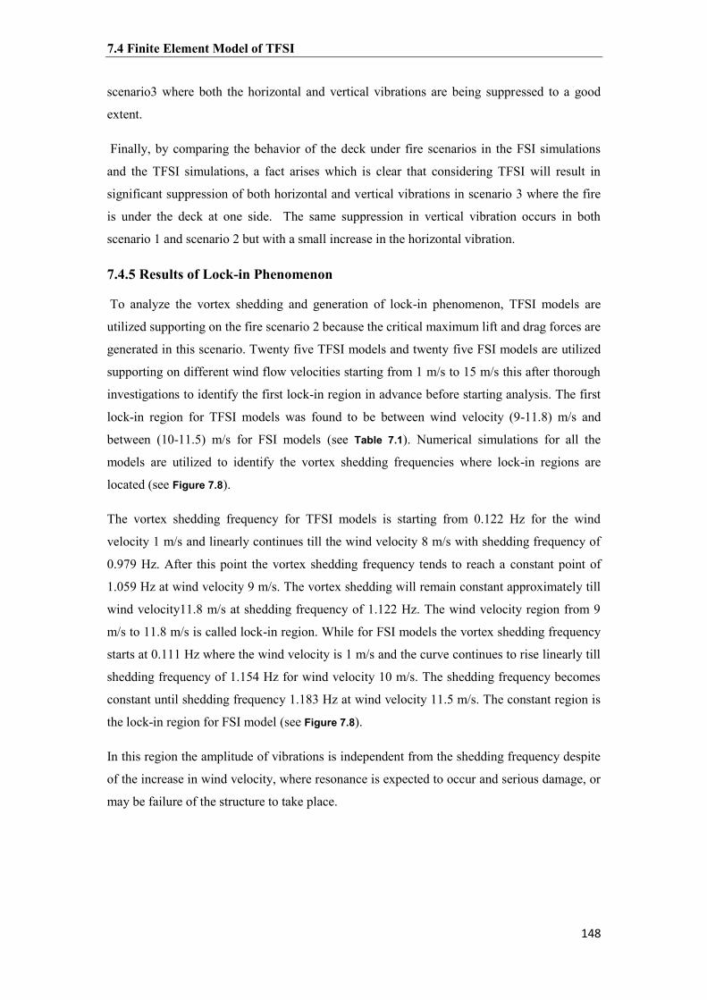
7.4 Finite Element Model of TFSI
148
scenario3 where both the horizontal and vertical vibrations are being suppressed to a good
extent.
Finally, by comparing the behavior of the deck under fire scenarios in the FSI simulations
and the TFSI simulations, a fact arises which is clear that considering TFSI will result in
significant suppression of both horizontal and vertical vibrations in scenario 3 where the fire
is under the deck at one side. The same suppression in vertical vibration occurs in both
scenario 1 and scenario 2 but with a small increase in the horizontal vibration.
7.4.5 Results of Lock-in Phenomenon
To analyze the vortex shedding and generation of lock-in phenomenon, TFSI models are
utilized supporting on the fire scenario 2 because the critical maximum lift and drag forces are
generated in this scenario. Twenty five TFSI models and twenty five FSI models are utilized
supporting on different wind flow velocities starting from 1 m/s to 15 m/s this after thorough
investigations to identify the first lock-in region in advance before starting analysis. The first
lock-in region for TFSI models was found to be between wind velocity (9-11.8) m/s and
between (10-11.5) m/s for FSI models (see Table 7.1). Numerical simulations for all the
models are utilized to identify the vortex shedding frequencies where lock-in regions are
located (see Figure 7.8).
The vortex shedding frequency for TFSI models is starting from 0.122 Hz for the wind
velocity 1 m/s and linearly continues till the wind velocity 8 m/s with shedding frequency of
0.979 Hz. After this point the vortex shedding frequency tends to reach a constant point of
1.059 Hz at wind velocity 9 m/s. The vortex shedding will remain constant approximately till
wind velocity11.8 m/s at shedding frequency of 1.122 Hz. The wind velocity region from 9
m/s to 11.8 m/s is called lock-in region. While for FSI models the vortex shedding frequency
starts at 0.111 Hz where the wind velocity is 1 m/s and the curve continues to rise linearly till
shedding frequency of 1.154 Hz for wind velocity 10 m/s. The shedding frequency becomes
constant until shedding frequency 1.183 Hz at wind velocity 11.5 m/s. The constant region is
the lock-in region for FSI model (see Figure 7.8).
In this region the amplitude of vibrations is independent from the shedding frequency despite
of the increase in wind velocity, where resonance is expected to occur and serious damage, or
may be failure of the structure to take place.

7.4 Finite Element Model of TFSI
149
Table 7.1
Lock-in data for TFSI and FSI models
TFSI models FSI models
Wind Velocity m/s
Vortex shedding frequency Hz
Vortex shedding frequency Hz
1 0.122 0.111
2 0.255 0.221
3 0.383 0.329
4 0.506 0.455
5 0.612 0.571
6 0.734 0.676
7 0.856 0.809
8 0.979 0.942
9 1.059 1.067
10 1.069 1.154
11 1.087 1.164
11.5 1.111 1.183
11.6 1.112 1.233
11.7 1.117 1.236
11.8 1.122 1.363
11.9 1.456 1.369
12 1.468 1.386
12.1 1.481 1.456
12.2 1.493 1.412
12.3 1.505 1.447
12.4 1.517 1.465
12.5 1.53 1.485
13 1.591 1.535
14 1.713 1.617
15 1.861 1.777
Figure 7.8 Lock-in Phenomenon - TFSI and FSI models
0 5 10 150
0.5
1
1.5
2
U [ m/s ]
Ns [
Hz
]
FSI-ModelTFSI-Model
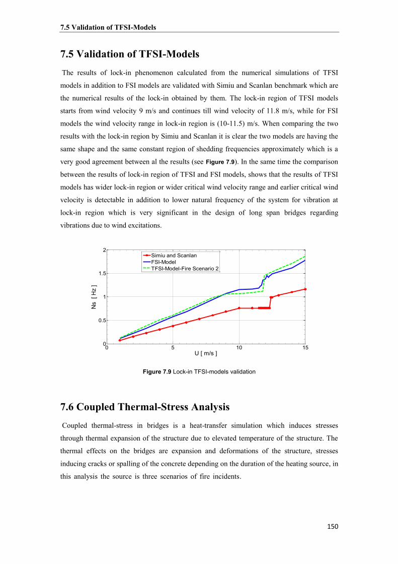
7.5 Validation of TFSI-Models
151
7.5 Validation of TFSI-Models The results of lock-in phenomenon calculated from the numerical simulations of TFSI
models in addition to FSI models are validated with Simiu and Scanlan benchmark which are
the numerical results of the lock-in obtained by them. The lock-in region of TFSI models
starts from wind velocity 9 m/s and continues till wind velocity of 11.8 m/s, while for FSI
models the wind velocity range in lock-in region is (10-11.5) m/s. When comparing the two
results with the lock-in region by Simiu and Scanlan it is clear the two models are having the
same shape and the same constant region of shedding frequencies approximately which is a
very good agreement between al the results (see Figure 7.9). In the same time the comparison
between the results of lock-in region of TFSI and FSI models, shows that the results of TFSI
models has wider lock-in region or wider critical wind velocity range and earlier critical wind
velocity is detectable in addition to lower natural frequency of the system for vibration at
lock-in region which is very significant in the design of long span bridges regarding
vibrations due to wind excitations.
Figure 7.9 Lock-in TFSI-models validation
7.6 Coupled Thermal-Stress Analysis Coupled thermal-stress in bridges is a heat-transfer simulation which induces stresses
through thermal expansion of the structure due to elevated temperature of the structure. The
thermal effects on the bridges are expansion and deformations of the structure, stresses
inducing cracks or spalling of the concrete depending on the duration of the heating source, in
this analysis the source is three scenarios of fire incidents. .
0 5 10 150
0.5
1
1.5
2
U [ m/s ]
Ns
[ H
z ]
Simiu and ScanlanFSI-ModelTFSI-Model-Fire Scenario 2

7.6 Coupled Thermal-Stress Analysis
151
Modeling of thermal-stress analysis or coupled problems in general [Zhuang et al., 2014]
poses significant challenges on the computational methods, particularly when coupled with
fluid-structure interaction and fracture. [Rabizadeh et al., 2016] proposed an adaptive FE
analysis for thermoelasticity problems in the context of the finite element method. Efficient
approaches to fracture include meshfree methods [Rabczuk et al., 2004; Rabczuk and
Belytschko, 2005; Amiri et al., 2014; Amiri et al., 2016] the extended finite element method,
phantom node methods [Rabczuk et al., 2008; Chau-Dinh et al., 2012; Vu-Bac et al., 2013],
extended meshfree methods [Rabczuk and Areias, 2000; Rabczuk and Belytschko, 2006;
Rabczuk et al., 2007; Zi et al., 2007; Rabczuk and Zi , 2007; Rabczuk et al., 2007; Bordas et
al., 2008; Rabczuk et al., 2008; Rabczuk et al., 2010; Amiri et al., 2014], efficient remeshing
techniques [Areias et al., 2013; Areias et al., 2013; Areias et al., 2013; Areias et al., 2015;
Areias et al., 2016], screen-Poisson models [Areias et al., 2016 and Areias et al., 2016],
cracking particles methods [Rabczuk and Belytschko, 2004; Rabczuk and Areias, 2006;
Rabczuk and Belytschko, 2007; Rabczuk et al., 2007; Rabczuk and Samaniego, 2008;
Rabczuk et al., 2010], anisotropic softening elements [Areias et al., 2014], extended IGA
[Ghorashi et al., 2015; Jia et al., 2015; Nguyen-Thanh et al., 2015; Quoc et al., 2016],
multiscale methods for fracture [Talebi et al., 2013; Budarapu et al., 2014; Silani et al., 2014;
Talebi et al., 2014; Budarapu et al., 2014; Talebi et al., 2015; Silani et al., 2016] and
peridynamics or dual-horizon peridynamics formulations [Vu-Bac et al., 2015; Amani et al.,
2016; Ren et al., 2016; Vu-Bac et al., 2016; Ren et al., 2017 ], to name a few though IGA and
XFEM has also been exploited for other applications [Nanthakumar et al., 2013; Valizadeh et
al., 2015; Nguyen et al., 2015; Anitescu et al., 2015; Nanthakumar et al., 2015; Ghasemi et
al., 2017; Chan et al., 2017; Rabczuk and Ren, 2017; Hamdia et al., 2017; Areias and
Rabczuk, 2017 ]. Fluid-structure interaction driven fracture has been proposed for instance in
[Rabczuk et al., 2010]. However, a coupled thermal stress analysis involving fluid-structure
interaction and fracture has not been carried out so far.
7.6.1 Thermal Cracking and Spalling of Concrete
Excessive differences in temperature within a concrete structure or its surrounding result in
thermal cracking. This causes contract of the cool part more than the warmer part and
consequently the contraction would be restrained. When the tensile stresses exceed the tensile
strength of the concrete, the thermal cracks appear. When extreme temperature differences
occur, thermal cracks with a random pattern appear on the concrete structural element.
Spalling is another aspect of thermal stresses inducing thermal strains which end with the
cracking and spalling of portions of concrete. The high temperature and intensity of the fire
causes bursting pressure in the moisture trapped within the microstructure of the concrete.
Due to unequal thermal expansion between the aggregates, cementitious paste and the steel

7.6 Coupled Thermal-Stress Analysis
152
bars can increase spalling of the concrete. In addition to material properties of the concrete,
geometric parameters like section shape and size contribute to the spalling of concrete.
Environmental parameters such as heating rate and profile, thermal restraint and temperature
level also affect the occurrence of spalling [Stratford and Dhakal, 2008; Bo, 2011; Ervine,
2012; Chung et al., 2013; Mueller and Kurama, 2014 and Klingsch, 2014].
Heating rates in the range of 20-32°C/min are significant for spalling to occur [Khoury,
2000]. The high heating rates occur in the early stages of the fire. Several researchers have
identified critical temperature ranges for spalling to start regarding exposed surface to fire.
[Akhtaruzzaman and Sullivan, 1970] have stated that exposed surface temperatures in the
range of 375 - 425°C for normal weight concretes leads to spalling. [Choi and Shin, 2011]
determined theoretically and experimentally the zone of spalling of a reinforced concrete
beam exposed to ISO 834 fire where the location of the spalling is at the upper right and left
of the external part of the beam.
7.6.2 Finite Element Model of Coupled Thermal-Stress
The full model of a cable stayed bridge is created in ABAQUS to undergo thermal stresses
due to heat transfer from a fire source for a long duration of 20 minutes supporting on the
standard ISO 834 Fire data. Three scenarios (the same as TFSI case) are dedicated to simulate
the effect of the fire on the deformations, cracks and spalling of concrete. A cable stayed
bridge model is created with 324 m length and 22 m width, the main parts of the bridge is the
deck which consists of connected reinforced concrete deck segments with 2.6 m height. Four
reinforced concrete pylons with square shapes 4*4 m dimensions and 103 m height, and 80
stay cables are connecting the deck to the pylons in a fan shape arrangement, each cable with
cross section area 0.00785 m2 (see Figure 7.10).
Figure 7.10 Finite element 3D model of the cable stayed bridge

7.6 Coupled Thermal-Stress Analysis
153
The main steel bar diameter is 0.06 m and the diameter of the temperature steel bars in
addition to the stirrups are 0.04 m. The boundary condition of the deck is fixed in one side
and free for longitudinal translation in the other side. The pylons are fixed at the bottom and
each two pylons are connected by six reinforced concrete ties with 4*4 m dimensions and 22
m length. The stay cables equivalent Young's modulus of elasticity has been used to
approximate the sagging occurrence in the cables because it was modeled as truss elements
(see Table 7.2). An ambient temperature of 293.15 K is assigned to the whole model, and a
static general step is created for duration of 1200 seconds. A predefined field (temperature
type) is assigned in to the region where three fire scenarios are considered with amplitude of
time dependent temperature (Standard ISO 834 Fire).
Table 7.2 Material properties
Material Mass Density Kg/m3
Young's Modulus of
Elasticity Pa Poisson's
Ratio Thermal
Conductivity W/m
2K
Specific Heat
J/kg.K
Concrete
2643
2.00E+10
0.20
2
890 Steel bar 7800 2.00E+11 0.30 20 490
Stay cable 9438 1.65E+11 0.30 21 460 To simulate the propagation of the cracks and the spalling in the concrete due to fire action,
equivalent thermal stresses are added in the fired regions using XFEM approach for each fire
scenario. Maximum principal stress is assigned in addition to the displacement at failure. The
start of damage in the simulations is identified with a maximum principal stress generated at
the temperature 400°C where the cracks and spalling in the concrete are prone to occur.
The deck is modeled as (C3D10: A10-quadratic tetrahedron) elements, pylons and ties are
modeled as (C3D8R: An 8 node linear brick reduced integration hourglass control) elements,
the reinforcing steel bars are modeled as (B31: A 2- node linear beam in space) elements and
the stay cables are modeled as (T3D2: A 2- node linear 3D truss) elements.
7.6.3 Results of Deck Displacements
Three fire scenarios for the duration of 1200 seconds on the middle part of the cable stayed
bridge in the region of (22*20) m is considered and the results of the displacements for each
case are calculated for a center point in the middle of the cable stayed bridge model.

7.6 Coupled Thermal-Stress Analysis
154
Considering the maximum horizontal displacements, this maximum value for scenario1 was
low which is reached 0.7 cm upward at the end of the 1200 seconds. While for scenario 2, this
maximum value was very low which is reached 0.02 cm upward at 172 seconds. Furthermore,
the maximum value for scenario3 was high reaching 20.4 cm downward at the end of the
1200 seconds of the fire exposition (see Figure 7.11).
Relating to the maximum vertical displacements, all the scenario cases reached teir
maximum values at the end of the fire exposition after 1200 seconds. Scenario 1 showed very
high maximum value of 44.2 cm upward. This maximum value for scenario2 was high
reached 33.7 cm downward but it is less than of it in the previous scenario. While for
scenario3, the maximum vertical displacement reache 18.1 cm downward which is less than
all the scenario cases ( see Figure 7.12). Finally, with respect to the maximum angular
displacemnts, all the scenarios reach the maximum value at the end of the 1200 seconds. In
scenario 1 , the maximum value was 0.038° which is considered very low which is not
effective. In the other hand , this value for scenario 2 was 0.064° which is nearly twice the
previous value but still not appreciable to induce stresses in the deck. While for scenario 3,
the maximum value reached 0.086° which is greater than all the maximum values in scenario
1 and scenario2 and is three times of the maximum value in scenario 1 approximately and it is
not an effective in producing stresses in the deck ( see Figure 7.13).
Figure 7.11 Horizontal displacement Figure 7.12 Vertical displacement
Figure 7.13 Angular displacement
0 200 400 600 800 1000 1200-1
-0.5
0
0.5
1
t [ s ]
Dis
pla
ce
me
nt
- V
ert
ica
l [
m ]
Fire Scenario 1Fire Scenario 2Fire Scenario 3
0 200 400 600 800 1000 1200
-0.25
-0.2
-0.15
-0.1
-0.05
0
0.05
0.1
0.15
t [ s ]
Dis
pla
ce
me
nt
- H
ori
zo
nta
l [
m ]
Fire Scenario 1Fire Scenario 2Fire Scenario 3
0 200 400 600 800 1000 1200
-0.1
-0.05
0
0.05
0.1
0.15
t [ s ]
Dis
pla
cem
en
t -
An
gu
lar
[ °
]
Fire Scenario 1Fire Scenario 2Fire Scenario 3

7.6 Coupled Thermal-Stress Analysis
155
This is an indication that the horizontal displacement in scenario 3 where the fire is exposed
on one side under the deck is the critical case in generating tension stresses in the fired side
and compression stresses in the opposite sides of the deck. The vertical displacement in
scenario 1 where the position of the fired region is above the deck is the critical case in
inducing tension stresses that are the reason of propagation of cracks and spalling of the
concrte above the deck whenever these stresses exceed the tensile strength of the concrete.
While the angular displacement in scenario 3 is the critical case but it is too low which is not
appreciated in the geneartion and propagation of cracks and spalling of concrete.
7.6.4 Extended Finite Elemnt Method
The extended finite element method (XFEM) is a partition of unity based numerical method.
It uses the partition of unity to describe the discontinuous displacement and uses the
enrichment function to realize the displacement jump over the discontinuity, see Equation
(7.15) which represents the discretization of the displacement field in 1D. The first term is the
continuous displacement while the second term is the discontinuous displacement.
( ) ∑
( ) ∑
( ) ( ( )) ( )
The classical finite element approximation is enhanced by means of enrichment functions.
The enrichment procedure is employed on a local level for the XFEM. Thus, only nodes close
to the crack tip, as well as the ones required for the correct localization of the crack, are
enriched. In the XFEM, enrichment functions are added to additional nodes, in order to
include information about discontinuities and singularities around the crack. These functions
are the asymptotic near-tip solutions, which are sensitive to singularities, and the Jump
function, which simulates the discontinuity when the crack opens. This evidently entails a
tremendous computational advantage. The XFEM method was firstly introduced by
[Belytschko and Black, 1999]. Their work, in which a method for enriching finite element
approximation in such a way that crack growth problems can be solved with minimal
remeshing, represents a milestone in the XFEM history. Later on, much more elegant
formulations, including the asymptotic near-tip field and the Heaviside function in the
enrichment scheme, have been proposed [Dolbow, 1999; Moes et al., 1999; Dolbow et al.,
2000]. The XFEM method, furthermore, has been demonstrated to be well suited for three
dimensional crack modelling [Sukumar et al., 2000]. Let's assume we have a crack in
element 2 between nodes 2 and 3. To capture the discontinuity, we multiply the FE shape
function with a so-called enrichment function. Since we know the displacement field is
discontinuous, we use a discontinuous enrichment function such as the step function. The

7.6 Coupled Thermal-Stress Analysis
156
Figure 7.14 shows the enriched shape functions of node 2 and node 3 which can be seen that
they are discontinuous across the crack.
Figure 7.14 Enriching shape functions of node 2 and node 3
Regarding the XFEM discretization of the temperature field due to fire, we assume that the
temperature is discontinuous across the crack and therefore we adopt the same enrichment
strategy as for the displacement field.
The XFEM capabilities can be extended if employed in conjunction with the level set method
(LSM) [Osher and Sethian, 1988; Stolarska et al., 2001; Ventura et al., 2003] which is a
technique for describing a crack and tracking the motion of the crack. The first level set
function describes the crack surface Ф (phi), the second level set function is constructed so
that the intersection of two level sets gives the crack front Ѱ (psi). Such method permits to
represent the 3D crack for both the position and the location of the crack tips (see Figure 7.15).
Figure 7.15 Crack in 3D by two level set functions

7.6 Coupled Thermal-Stress Analysis
157
7.6.5 Results of Cracking and Spalling of The Deck
To identify the damaged regions in the cable stayed bridge model, maximum principal stress
values calculated in ABAQUS are used for damage detection with the support of XFEM to
simulate the propagation of the cracks and occurrence of spalling in the concrete. In all fire
scenarios the duration of the fire is 20 minutes supported on standard ISO 834 Fire data.
In fire scenario 1, the fired region is shown (see Figure 7.16). Cracks and spalling of concrete
can be seen at the middle and external edges of deck (see Figure 7.17). The cracks propagated
from the inner edges of the flange toward the external edges leading to occurrence of spalling.
This is due to high vertical displacement upward and angular displacement of the deck caused
by the thermal stresses which induced high tensile stresses in the concrete exceeded the
tensile strength of the concrete.
Figure 7.16 Maximum principal stress - Fire scenario 1- Without XFEM damage simulation
Figure 7.17 Maximum principal stress - Fire scenario 1- With XFEM damage simulation

7.6 Coupled Thermal-Stress Analysis
158
Considering fire scenario 2, the fired region is shown in (Figure 7.18). Cracks are obvious in
the web of the deck in addition to spalling of concrete at one side of the exterior edges (see
Figure 7.19). The cracks appear first at the middle and the external edges of the web, then they
propagate from the exterior edges toward middle part of the web and consequently spalling
occurs. The thermal stresses generated high vertical displacement downward and relative
higher angular displacement of the deck with respect to its value in sceanrio1.
Figure 7.18 Maximum principal stress - Fire scenario 2- Without XFEM damage simulation
Figure 7.19 Maximum principal stress - Fire scenario 2- With XFEM damage simulation
While for fire scenario 3, the fired region is shown in (Figure 7.20). Cracks with spalling of
concrete can be seen at one side of the exterior edges on the web (see Figure 7.21). The cracks
start first at the fired side and then they propagate toward the middle of the web and as a
result, spalling occurs.

7.6 Coupled Thermal-Stress Analysis
159
Figure 7.20 Maximum principal stress - Fire scenario 3- Without XFEM damage simulation
Figure 7.21 Maximum principal stress - Fire scenario 3- With XFEM damage simulation
Cracks and spalling of concrete occur in all fire scenarios due to high temperature exposure
of the deck. Consequently the highest damage in the deck of the cable stayed bridge takes
place in the fire scenario1 where the fire is above the deck because larger amounts of cracks
and spalling appear in earlier time from the fire incident and the failure of the structure is
more prone to occur compared to other two fire scenarios.

7.7 Validation of Coupled Thermal-Stress Models
161
7.7 Validation of Coupled Thermal-Stress Models Von Mises stress of the concrete is utilized as the criteria of failure detection in a concrete
structure, which is used to visualize the location and magnitude of the deck crack and spalling
due to fire exposition. To validate the models of the spalling and cracking of the deck, a
benchmark of the spalling zone of the reinforced concrete beam by Choi and Shin, 2011 is
dedicated. The zone of the cracks and spalling of concrete of the coupled thermal-stress
models are in the upper external sides of the deck at the mid span of the cable stayed bridge
model in all three fire scenarios. Comparing the two results indicates that there is a good
agreement between the results of the coupled thermal-stress models and the results of the
benchmark model.

161

162
Chapter 8
Conclusions and Recommendations for Further Researches
8.1 Conclusions The application of ABAQUS finite element program to study the assessment of CSD, CFD
and coupled models of wind-induced vibrations and control efficiency in long span cable
supported bridges has shown great capabilities in identifying the predicted vertical and
torsional vibrations and the associated critical wind speeds. The results confirmed the
robustness of the approach in detecting the actual predicted VIV and lock-in phenomenon by
utilizing the FSI concept. Another strength aspect of this work was optimizing the application
of the MTMDs to suppress the vertical and torsional vibrations of the deck and the control
efficiency of this method was high relatively compared to the previous results from the
benchmarks in the literature. It is worthy to mention that employment of surrogate modeling
supporting on many experimental sampling methods in addition to Sobol’s global sensitivity
indices method identified and detected the predicted roles and rational effects of eight certain
and uncertain aerodynamic parameters which are considered the main sources of the
aerodynamic stability of the long span cable supported bridges. Frequency analysis helped to
identify the natural frequencies of the structure which are related to the vibration modes, in
addition to recognizing the dangerous coupling between the vertical and the torsional
vibrations. Structural modification was conducted and consequently, the vertical and torsional
stiffness of the structure were increased. Also the danger of coupling was removed to higher
natural frequencies which are rarely happen. Furthermore, a safer structural performance was
obtained. The application of TFSI concept exhibited high accuracy and capability to simulate
and analyze the effect of triple coupling between the wind and the deck domains in addition
to the thermal boundary. It succeeded to predict the early generation of VIV and lock-in
phenomena, also revealed the role of temperature field in the behavior of the cable stayed
bridge during wind excitations and fire incidents together.The coupled thermal-stress analysis
manifested very well in predicting the thermal deformations of the deck in addition to the
damages detection regarding the generation of cracks and spalling of the concrete due to fire
exposure with the support of XFEM analysis application.

8.1 Conclusions
163
All the mentioned results are formulating significant backgrounds to pave the way to the
engineers in that field to insure preparing better design with a greater factor of safety against
vibrations risks and the danger of structural failure in addition to wide region of modification
solutions to control the early weakness in the behavior and performance of long span cable
supported bridges under wind actions.
The following axes are the summary of the conclusions in details:
1- The numerical simulations in conjunction with frequency analysis confirmed the existence
of vertical and torsional vibrations of the deck due to wind excitation which is being
considered as a basic reference to understand the buffeting response and flutter instability of
the cable stayed bridge, and the results of the vortex shedding from the deck of the long span
bridge showed that the two-way FSI approach is more efficient than the one-way FSI
approach in detecting the generation of earlier VIV and predicting lower critical wind
velocities as a result detecting earlier lock-in phenomenon, which are indications for
designers to avoid the VIV in the design stage by ensuring that the frequencies of the vortices
generated are sufficiently separated from the natural frequencies of the long span bridge by
altering the geometrical design of the deck or changing the natural frequencies of the system.
The results of lift forces generated in the deck of the long span bridge in the two-way FSI
approach is smaller than the same values for the one-way FSI approach, which means that the
two-way approach determines the actual magnitude of the energy dissipation for the VIV of
the deck and the vertical periodic oscillation of the deck is detected in lower wind velocities
only by utilizing two-way FSI approach. Supporting on these results, the cable stayed bridge
is designed safely through avoiding wrong estimation of late VIV where in some cases lead to
resonant and dangerous events.
2- Eight certain and uncertain aerodynamic parameters have been optimally identified their
values that are responsible of improving the aerostatic and aerodynamic instabilities of the
cable stayed bridge. The wind attack angle and wind speed parameters were the most
effective parameters that affected the buffeting response and the flutter instability in addition
to generation of vortex shedding. The deck streamlined length parameter demonstrated a
nonlinear effect for a certain deck shape which falls between a bluff shape and a streamlined
shape which was an optimum case that supports the generation of vortex shedding and the
oscillation of the deck. The dynamic viscosity of air parameter has a nonlinear effect on the
vortex shedding and the vertical oscillations of the deck, where increasing this parameter to
high values will enhance the generation of the vortex shedding due to energy dissipation
mechanism.The viscous damping of the stay cable parameter showed a nonlinear relation with
the vertical vibration of the deck. When this parameter is increased, the displacement at the

8.1 Conclusions
164
center of the deck mid-span decreased in a small range with irregular pattern. While for
torsional vibration of the deck, a very small non appreciable effect on the flutter displacement
of the deck was seen. The mass ratio parameter that is related to the TMDs has a nonlinear
effect on the vertical vibration control efficiency and linear effect on the torsional vibration
control efficiency. Commonly increasing this ratio to a limited range will decrease both the
vertical and torsional vibrations of the deck in an appreciable amount. The frequency ratio
parameter has a semi linear effect on the vertical vibration control efficiency and linear effect
on the torsional vibration control efficiency. Where increasing this parameter value in a
bound limit, will decrease the vertical vibration of the deck in acceptable rate. While
increasing this parameter value has a nonappreciable effect on the torsional vibration. Finally
the damping ratio parameter has a linear effect on the vertical vibration control efficiency and
linear effect on the torsional vibration control efficiency. Where increasing this parameter
value in a bound limit, will decrease the vertical vibration of the deck with a small rate, and
has a very small effect on the torsional vibration which can be neglected.
3- Global sensitivity analysis for the aerodynamic parameters formulated surrogate models
which were supported on Monte Carlo sampling method to predict the buffeting response and
flutter instability of the cable stayed bridge so that to dedicate suitable plans and solutions for
each vibration case thoroughly. Latin hypercube sampling method established efficient
surrogate models to calculate the predicted kinetic energy of the system and the lift forces that
are the background data to analyze and control the generation of VIV. Box-Behnken
experimental method formulated excellent surrogate models representing the actual response
of the system to efficiently calculate the performance of the MTMDs in suppressing both the
vertical and torsional vibrations of the deck.
4- The sensitivity indices revealed the rational effect and role of each aerodynamic parameter
on the aerodynamic instability of the structure which are considered important data to identify
the priorities in the design procedure so that to optimize the response of the system against
vertical and torsional vibrations of the deck which are resulting due to strong critical wind
excitations.The role and the rational effects of wind attack angle parameter were very high on
both the vertical and torsional vibrations of the deck. The uncertainty of this parameter has
been identified to a good range which is responsible directly on the aerodynamic instability of
the structure.While the role and the rational effects of the deck streamlined length parameter
was not important related to the kinetic energy of the system, while it was effective on the
generation of lift forces due to VIV and buffeting response. Cconsequently a good
consideration should be given to this parameter. Related to the rational effects of the stay
cables viscous damping parameter, it is clear that this parameter has a fair effect on the
vertical vibration and a good effect on the torsional vibration, as a result the uncertainties of

8.1 Conclusions
165
this parameter are well studied.The role and the rational effects of wind speed parameter were
very high on the kinetic energy of the system and the lift forces and this parameter should be
considered for uncertainties in the generation of vortex shedding and oscillation of the deck
due to VIV and flutter instability. In the other hand, the dynamic viscosity of air parameter
has a non appreciable rational effect on the kinetic energy of the system, and has a small
rational effect on the lift forces, hence the uncertainties related to this parameter on the vortex
shedding and oscillation of the deck is very small. Furthermore, the rational effect of the mass
ratio on the vertical vibration was high and on the torsional vibration was too much high,
where this parameter can be considered the source of torsional control efficiency. While the
rational effect of the frequency ratio parameter on the vertical vibration was low and no effect
at all on the torsional vibration. Mreover, the rational effect of the damping ratio parameter on
the vertical vibration was too much low and no effect on the torsional vibration.
5- The novel structural modification of the cable stayed bridge model succeeded to increase
the bending and torsional stiffness of the structure to a wide range in such a way that showed
larger efficiency as vibrations suppressor compared to other approaches that have been
adopted for vibrations control in long span bridges such as TMDs, Sealed tuned liquid column
gas dampers and electromechanical actuator.The natural frequencies of the system were
modified positively, where the flutter wind speed has been modified to larger magnitudes, and
it insured the safety of the structure against a dangerous coupling between the vertical and
torsional mode shapes of vibrations by altering the coupling mode shape to much higher
natural frequencies after structural modification, which is an indication that the safety of the
structure against vertical and torsional vibrations and the coupling between them has been
guaranteed to a large factor of safety.
6- When TFSI numerical simulations are adopted, nonlinear behavior is detected for the deck
under fire scenario 1 and fire scenario 2 regarding the horizontal and vertical vibrations of the
deck which imposes special analysis for each case up to the design needs and specifications of
safety against vibrations. While for fire scenario 3 a significant suppression of both horizontal
and vertical vibrations to a good level has been identified. This fact can be further utilized to
use heating sources to invent new devices for the suppressing vibrations in long span bridges
where the lower temperature that enhances that target is lower than 100°C supporting on the
results of lift and drag forces for fire scenario 3 and the standard ISO 834 fire curve. An
earlier critical wind velocity is discovered for the TFSI simulations in the same time lower
vortex shedding frequencies for fire scenario 2 where the fire is under the deck, which
enhances the generation of earlier VIV and earlier lock-in phenomenon which is a serious
matter related to the service ability and safety of the cable stayed bridge due to vibrations and
failure. As a result a special attention should be dedicated to prevent

8.2 Recommendations for Further Researches
166
heating of the deck (above part) especially in hot countries where the source of heating from
the environment helps this situation. Using both coupled thermal-stress and XFEM
simulations, all fire scenarios generated thermal stresses in the deck due to very high
temperature, consequently deformations and damage of the concrete comprising cracks and
spalling of the concrete, especially fire scenario 1 where larger amounts of cracks and spalling
appear earlier which is considered critical for the safety of the structure compared to ire
scenario 2 and fire scenario 3.
8.2 Recommendations for Further Researches Supporting on the conclusions and the capability of model assessment by the finite element
method and the sensitivity analysis approach, it is recommended to further widening the
scope of the researches in this area by conducting the following investigations:
1- Using different models for the segmental decks such as circular and trapezoidal shapes so
that to investigate the buffeting response and flutter instability of the long span cable
supported bridge, where certain structural shapes are highly decisive in generating vibrations.
2- Considering higher wind speeds for CFD simulations more than 25 m/s so that to discover
higher critical wind speeds which are responsible of higher shedding frequencies related to far
lock-in regions, where the computational efforts and cost are higher compared to lower winds
speeds cases. This helps to secure placing the design of the deck away from vortex induced
vibration in very strong winds situations.
3- Designing the MTMDs with various shapes and dimensions in addition to positioning them
in different places in the deck so that to optimize their effects on controlling both the vertical
and torsional vibrations of the deck. Also a combination of both MTMDs and viscous
dampers is recommended, where this method in certain cases might be effective in enhancing
the suppression of the vibrations.
4- Modeling the stay cables with other shapes of distributions, such as semi fan shapes and
harp shapes to search the robustness of the structural modification for damping consideration,
where the local and the global responses even the coupled responses of the long span cable
supported bridges are associated with the motions and the quasi static motions of the stay
cables.
5- Investigating other uncertain parameters such as horizontal skewedness of the wind effect
on the buffeting response and flutter instability of the structure, in addition to its effect on the
vortex shedding and lock-in phenomenon, where in most of research studies this parameter is
not considered due to complexity of modeling the wind profile in finite element method.

8.2 Recommendations for Further Researches
167
6- Adopting different sampling methods like (LP-TAU) to search the results of the surrogate
models of the predicted response of the structure for vibrations control, and supporting on
other sensitivity analysis methods such as analysis of variance (ANOVA) and Fourier
Amplitude Sensitivity Test (FAST) to calculate the effect of the parameters on the aerostatic
and aerodynamic stability of the structure, in addition to comparison process between these
methods to identify the most critical method in that direction.
7- Starting global sensitivity analysis in thermal fluid-structure interaction simulations
utilizing transient heat-transfer of a fire considering input parameters such as heating rate,
heat flux, concrete density, ambient temperature and wind speed so that to identify the role
and rational effect of each parameter on the behavior of the deck during fire incidents.

Appendix A
168
Appendix A
A.1 Mesh Convergence
Figure A.1 Mesh convergence for mode shapes of vibrations
A.2 Surrogate Models Equations for Vertical and Torsional Responses (MATLAB Codes)
Yv = -0.020883722+0.00010033145755*x1.*1-0.004164325912621*x2.*1+0.349777764990117*x3.*1-0.000001157304765*x1.^2+0.000496530180774*x2.^2-40.802891600598*x3.^2+0.00002158455372*x1.*x2-0.007290619361827*x1.*x3+0.375075585195514*x2.*x3 (A.2-1)
Yt = 0.00066213+0.000071351888482*x1.*1-0.000614461247787*x2.*1+0.429585797605989*x3.*1-0.000001098266034*x1.^2+0.000214156053979*x2.^2-12.998644305948*x3.^2+0.000013018552105*x1.*x2- 0.006775003312961*x1.*x3-0.047574577127205*x2.*x3 (A.2-2)
1 1.5 2 2.5 3 3.5 4 4.5 5 5.5 6x 10⁵
0.1
0.2
0.3
0.4
0.5
0.6
0.7
0.8
0.9
Number of Elements
Nat
ural
Fre
quen
cy [
Hz
]
Mode shape 2Mode shape 4Mode shape 6Mode shape 7

Appendix A
169
A.3 Lift Force and Aerodynamic Parameters
Figure A.3.1 Effect of wind speed on the generated lift force in the deck
Figure A.3.2 Effect of deck streamlined length on the generated lift force in the deck
Figure A.3.3 Effect of air dynamic viscosity on the generated lift force in the deck
0 10 20 30 40 50 60 70 80 90 1000
500
1000
1500
2000
2500
3000
t [ s ]
Fl [
N ]
Deck Streamlined Length L = 0 mDeck Streamlined Length L = 1 mDeck Streamlined Length L = 2 m
0 10 20 30 40 50 60 70 80 90 1000
5000
10000
15000
t [ s ]
Fl [
N ]
Air Dynamic Viscosity mu = 1.632E-5Air Dynamic Viscosity mu = 1.757E-5Air Dynamic Viscosity mu = 1.882E-5
0 10 20 30 40 50 60 70 80 90 100
0
1
2
3
4
5
6
7
8x 10⁶
t [ s ]
Fl [
N ]
wind speed v = 0.5 m/swind speed v = 12.5 m/swind speed v = 25 m/s

Appendix A
171
A.4 Surrogate Models Equations for Kinetig Energy and Lift Force (MATLAB Codes)
Yke = 909.283-18.142*X1.*1+18.548*X2.*1-96380686.352*X3.*1+36.486*X1.^2-26.663*X2.^2+2537569337783.03*X3.^2+2.891*X1.*X2+954150.697*X1.*X3+615868.57*X2.*X3 (A.4-1)
Yfl = -15665.09+256*X1.*1+135.69*X2.*1+1631247932.54*X3.*1+2*X1.^2-457.43*X2.^2-43018934785069.2*X3.^2-16.9*X1.*X2-11417513.33*X1.*X3+36495311.07*X2.*X3 (A.4-2)
A.5 Effect of TMD’s Design Parameters on Vertical and Torsional Responses
Figure A.5.1 Effect of TMD mass ratio on the vertical vibration of the deck
Figure A.5.2 Effect of TMD mass ratio on the torsional vibration of the deck
0 5 10 15 20 25 30-0.1
-0.08
-0.06
-0.04
-0.02
0
0.02
0.04
0.06
t [ s ]
d [ m
]
Without TMDTMD Mass Ratio u = 0.0025TMD Mass Ratio u = 0.0075TMD Mass Ratio u = 0.0125TMD Mass Ratio u = 0.0175TMD Mass Ratio u = 0.0225
0 5 10 15 20 25 30-0.08
-0.06
-0.04
-0.02
0
0.02
0.04
0.06
t [ s ]
d [ m
]
Without TMDTMD Mass Ratio u = 0.0025TMD Mass Ratio u = 0.0075TMD Mass Ratio u = 0.0125TMD Mass Ratio u = 0.0175TMD Mass Ratio u = 0.0225

Appendix A
171
Figure A.5.3 Effect of TMD frequency ratio on the vertical vibration of the deck
Figure A.5.4 Effect of TMD frequency ratio on the torsional vibration of the deck
Figure A.5.5 Effect of TMD damping ratio on the vertical vibration of the deck
0 5 10 15 20 25 30-0.08
-0.06
-0.04
-0.02
0
0.02
0.04
0.06
t [ s ]
d [ m
]
Without TMDTMD Frequency Ratio f = 0.8TMD Frequency Ratio f = 0.9TMD Frequency Ratio f = 1.0TMD Frequency Ratio f = 1.1TMD Frequency Ratio f = 1.2
0 5 10 15 20 25 30-0.08
-0.06
-0.04
-0.02
0
0.02
0.04
0.06
t [ s ]
d [ m
]
Without TMDTMD Frequency Ratio f = 0.8TMD Frequency Ratio f = 0.9TMD Frequency Ratio f = 1.0TMD Frequency Ratio f = 1.1TMD Frequency Ratio f = 1.2
0 5 10 15 20 25 30-0.06
-0.05
-0.04
-0.03
-0.02
-0.01
0
0.01
0.02
t [ s ]
d [ m
]
Without TMDTMD Damping Ratio d = 0.01TMD Damping Ratio d = 0.05TMD Damping Ratio d = 0.1TMD Damping Ratio d = 0.15TMD Damping Ratio d = 0.2
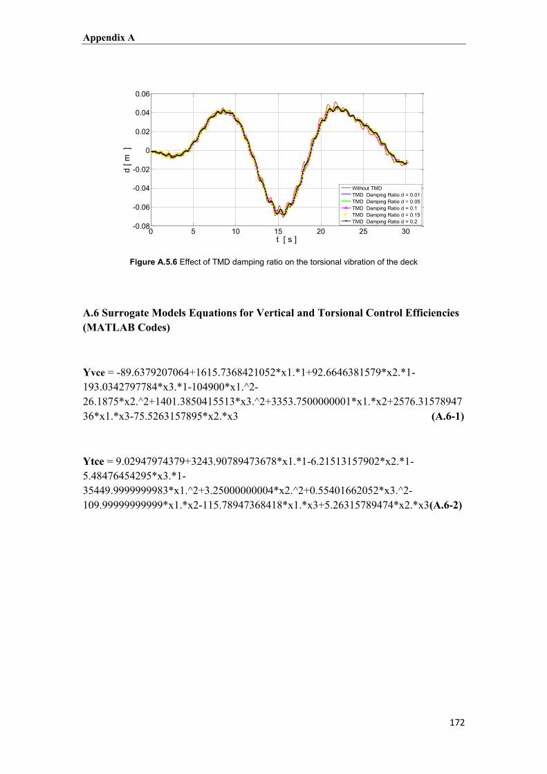
Appendix A
172
Figure A.5.6 Effect of TMD damping ratio on the torsional vibration of the deck
A.6 Surrogate Models Equations for Vertical and Torsional Control Efficiencies (MATLAB Codes)
Yvce = -89.6379207064+1615.7368421052*x1.*1+92.6646381579*x2.*1-193.0342797784*x3.*1-104900*x1.^2-26.1875*x2.^2+1401.3850415513*x3.^2+3353.7500000001*x1.*x2+2576.3157894736*x1.*x3-75.5263157895*x2.*x3 (A.6-1)
Ytce = 9.02947974379+3243.90789473678*x1.*1-6.21513157902*x2.*1-5.48476454295*x3.*1-35449.9999999983*x1.^2+3.25000000004*x2.^2+0.55401662052*x3.^2-109.99999999999*x1.*x2-115.78947368418*x1.*x3+5.26315789474*x2.*x3(A.6-2)
0 5 10 15 20 25 30-0.08
-0.06
-0.04
-0.02
0
0.02
0.04
0.06
t [ s ]
d [ m
]
Without TMDTMD Damping Ratio d = 0.01TMD Damping Ratio d = 0.05TMD Damping Ratio d = 0.1TMD Damping Ratio d = 0.15TMD Damping Ratio d = 0.2

References
173
References
Ab Kadir M. A. (2013). Fire Resistance of Earthquake Damaged Reinforced Concrete Frames. PhD
Thesis - The University of Edinburgh, Edinburgh, UK.
Abdel Raheem S. E. and Hayashikawa T. (2008). Vibration and Damping Characteristics of Cable-
Stayed Bridges Tower Control. International Association for Bridge and Structural Engineering, 8,
30 - 37.
Abdel-Aziz A. and Attia W. A. (2008). Aeroelastic Investigation of Different Deck Sections for
Suspension Bridges by Numerical Analysis. International Journal of Engineering and Innovative
Technology (IJEIT), 4(12), 49 - 57.
Abdi I. A., Abdulrahim A., Haser S., Uzol O. and Kurc O. (2012). Experimental and Numerical
Investigation of Wind Effects on Long Span Bridge Decks. 10th International Congress on Advances
in Civil Engineering, Ankara, Turkey. 17-19 October 2012.
Agar T. T. A. (1989). Aerodynamic Flutter Analysis of Suspension Bridges by a Modal Technique.
Engineering Structures, 11, 75 - 82.
Akhtaruzzaman, A. A. and Sullivan P. J. (1970). Explosive Spalling of Concrete Exposed to High
Temperature. Concrete Structures and Technology Research Report. London, Imperial.
Al-Assaf A. (2006). Flutter Analysis of Open-Truss Stiffened Suspension Bridges Using Synthesized
Aerodynamic Derivatives. PhD Thesis - Department of Civil and Environmental Engineering,
Washington State University, Washington, USA.
Allam S. M., Elbakry H. M. F. and Rabeai A. G. (2013). Behavior of One-Way Reinforced Concrete
Slabs Subjected to Fire. Alexandria Engineering Journal. 52, 749 - 761.
Alos-Moya J., Paya-Zaforteza I., Garlock M., Loma-Ossorio E., Schiffner D. and Hospitaler A.
(2014). Analysis of a Bridge Failure Due to Fire Using Computational Fluid Dynamics and Finite
Element Models. Engineering Structures, 68, 96 - 110.
Amani J., Oterkus E., Areias P. M. A., Zi G., Nguyen-Thoi T. and Rabczuk T. (2016). A non-
ordinary state-based peridynamics formulation for thermoplastic fracture. International Journal of
Impact Engineering, 87, 83 - 94.
Amenaghawon N.A., Nwaru K. I., Aisien F. A., Ogbeide S. E. and Okieimen C. O. (2013).
Application of Box-Behnken Design for the Optimization of Citric Acid Production from Corn Starch
Using Aspergillus Niger. British Biotechnology Journal, 3(3), 236 - 245.

References
174
Amiri F., Anitescu C., Arroyo M., Bordas S. and Rabczuk T. (2014). XLME interpolants, a seamless
bridge between XFEM and enriched meshless methods. Computational Mechanics, 53(1), 45 - 57.
Amiri F., Millan D., Arroyo M., Silani M. and Rabczuk T. (2016). Fourth order phase-field model
for local max-ent approximants applied to crack propagation. Computer Methods in Applied
Mechanics and Engineering, 312(C), 254 - 275.
Amiri F., Millán D., Shen Y., Rabczuk T. and Arroyo M. (2014). Phase-field modeling of fracture in
linear thin shells. Theoretical and Applied Fracture Mechanics, 69, 102 - 109.
Andersen M. S., Sahin E., Laustsen B., Lenius M. and Læso Jesper R. (2014). Implementation of
the Non-Flutter Design Principle. XIII Conference of the Italian Association for Wind Engineering IN-
VENTO 2014, Genova, Italy. 22-25 June 2014.
Andersson A., Connor A. O. and Karoumi R. (2013). External Damping of Stay Cables Using
Adaptive and Semi-Active Vibration Control. 8th International Cable Supported Bridge Operators
Conference, Edinburgh, UK. 3-5 June 2013.
Andersson C. and Ahl D. (2011). Fluid Structure Interaction Evaluation of Two Coupling Techniques.
M.Sc Dissertation - School of Information Science, Computer and Electrical Engineering, Halmstad
University, Halmstad, Germany.
Andrianne T. (2012). Experimental and Numerical Investigations of the Aeroelastic Stability of Bluff
Structures. PhD Thesis - Department of Aerospace and Mechanics, University of Liege, Liege,
Belgium.
Anitescu C., Jia Y., Zhang Y. and Rabczuk T. (2015). An isogeometric collocation method using
superconvergent points. Computer Methods in Applied Mechanics and Engineering, 284, 1073 -1097.
Annadurai G., Sung S. S. and Lee D. L. (2004). Optimisation of Floc characteristics for Treatment of
Highly Turbid Water. Separation Science and Technology, 39(1), 19 - 42.
Areias P. and Rabczuk T. (2013). Finite strain fracture of plates and shells with configurational forces
and edge rotation. International Journal for Numerical Methods in Engineering, 94(12), 1099 - 1122.
Areias P. and Rabczuk T. (2017). Steiner-point free edge cutting of tetrahedral meshes with
applications in fracture. Finite Elements in Analysis and Design, 132, 27 - 41.
Areias P. M. A., Rabczuk T. and Camanho P. P. (2014). Finite strain fracture of 2D problems with
injected anisotropic softening elements. Theoretical and Applied Fracture Mechanics, 72, 50 - 63.
Areias P., Msekh M. A. and Rabczuk T. (2016). Damage and fracture algorithm using the screened
Poisson equation and local remeshing. Engineering Fracture Mechanics, 158, 116 - 143.
Areias P., Rabczuk T. and Camanho P. P. (2013). Initially rigid cohesive laws and fracture based on
edge rotations. Computational Mechanics, 52(4), 931 - 947.

References
175
Areias P., Rabczuk T. and De Sá J. C. (2016). A novel two-stage discrete crack method based on the
screened Poisson equation and local mesh refinement. Computational Mechanics, 58(6), 1003 - 1018.
Areias P., Rabczuk T. and Dias-da-Costa D. (2013). Element-wise fracture algorithm based on
rotation of edges. Engineering Fracture Mechanics, 110, 113 - 137.
Areias P., Rabczuk T. and Msekh M. (2016). Phase-field analysis of finite-strain plates and shells
including element subdivision. Computer Methods in Applied Mechanics and Engineering, 312(C),
322 - 350.
Areias P., Reinoso J., Camanho P. and Rabczuk T. (2015). A constitutive-based element-by-element
crack propagation algorithm with local mesh refinement. Computational Mechanics, 56(2), 291 - 315.
Aslan N. and Cebeci Y. (2007). Application of Box-Behnken Design and Response Surface
methodology for modeling of some Turkish coals. Fuel, 86(1 - 2), 90 - 97.
Asyikin M. T. (2012). CFD Simulation of Vortex Induced Vibration of a Cylindrical Structure. M.Sc.
Dissertation - Department of Civil and Transport Engineering, Norwegian University of Science and
Technology, Trondheim, Norway.
Baba S., Kajita T. and Ninomiya K. (1988). Fire Under a Long Span Bridge. 13 th International
Association for Bridge and Structural Engineering (IABSE) congress, Helsinki. 6-10 June 1988.
Badia S. and Codina R. (2007). On Some Fluid Structure Iterative Algorithms Using Pressure
Segregation Methods: Application to Aeroelasticity. International Journal for Numerical Methods in
Engineering, 72, 46 - 71.
Bakis K. N., Massaro M., Williams M. S. and Limebeer D. J. N. (2016). Aeroelastic Control of
Long-Span Suspension Bridges with Controllable Winglets. Journal of Structural Control and Health
Monitoring, DOI: 10.1002/stc.1839.
Bakkiyaraj R. A. and Kumarappan N. (2013). Reliability Evaluation of Composite Electric Power
System Based On Latin Hypercube Sampling. International Journal of Electrical, Robotics,
Electronics and Communications Engineering, 7(4), 245 - 250.
Bandivadekar T. P. and Jangid R. S. (2012). Mass Distribution of Multiple Tuned Mass Dampers for
Vibration Control of Structures. International Journal of Civil and Structural Engineering, 3(1), 70 -
84.
Baroni G. and Tarantola S. (2014). A General Probabilistic Framework for Uncertainty and Global
Sensitivity Analysis of Deterministic Models: A Hydrological Case Study. Environmental Modelling
and Software, 51, 26 - 34.

References
176
Bartoli, G., Asdia, P., Febo, S., Pasto, C. and Procino, L. (2008). Innovative Solutions for Long-Span
Suspension Bridges. BBAA VI International Colloquium on: Bluff Bodies Aerodynamics and
Applications. Milano, Italy. 20-24 July 2008.
Behrens B. A., Krimm R. and Hasselbusch T. (2013). Tuned Mass Damper With Piezoelectrically
Tunable Damping. 20th International Congress on Sound and Vibration (ICSV20), Bangkok,
Thailand. 7-11 July 2013.
Belloli M., Fossati F., Giappino S. and Muggiasca S. (2014). Vortex Induced Vibrations of a Bridge
Deck: Dynamic Response and Surface Pressure Distribution. Journal of Wind Engineering and
Industrial Aerodynamics, 133, 160 - 168.
Belytschko T. and Black T. (1999). Elastic crack growth in finite elements with minimal remeshing.
International Journal for Numerical Methods in Engineering, 45(5), 601 - 620.
Bennetts I. and Moinuddin K. (2009). Evaluation of the Impact of Potential Fire Scenarios on
Structural Elements of a Cable-Stayed Bridge. Journal of Fire Protection Engineering, 19(4), 85 -
106.
Benra F. K., Dohmen H. J., Pei J., Schuster S. and Wan B. (2011). A Comparison of One-Way and
Two-Way Coupling Methods for Numerical Analysis of Fluid-Structure Interactions. Journal of
Applied Mathematics, 853560, 1 - 16.
Bienkiewicz, B. (1987). Wind Tunnel Study of Effects of Geometry Modification on Aerodynamics of a
Cable Stayed Bridge Deck. Journal of Wind Engineering and Industrial Aerodynamic, 26(3), 325 -
339.
Birken P., Gleim T, Kuhl D. and Meister A. (2015). Fast Solvers for Unsteady Thermal Fluid
Structure Interaction. International Journal for Numerical Methods in Fluids, 79(1), 16 - 29.
Blackburn H. and Henderson R. (1996). Lock-in Behavior in Simulated Vortex –Induced Vibration.
Journal of Experimental Thermal and Fluid Science, 12, 184 - 189.
Bo S. (2011). Finite Element Simulation of Fire Induced Spalling in High Strength Concrete Slabs.
M.Sc. Dissertation - Department of Civil and Environmental Engineering, Lehigh University,
Pennsylvania, USA.
Bonisch S., Dunne T. and Rannacher R. (2008). Numerics of Fluid-Structure Interaction.
Hemodynamical Flows, Modeling, Analysis and Simulation, 37, 333 - 378.
Bordas S., Rabczuk T. and Zi G. (2008). Three-dimensional crack initiation, propagation, branching
and junction in non-linear materials by an extended meshfree methods without asymptotic enrichment.
Engineering Fracture Mechanics, 75(5), 943 - 960.

References
177
Borna A., Habashi W. G., McClure G. and Nadarajah S. K. (2013). CFD-FSI Simulation of Vortex-
Induced Vibrations of a Circular Cylinder with Low Mass-Damping. Journal of Wind and Structures,
16(5), 411 - 431.
Bosch H. R. and Dhall T. (2008). Aerodynamic Investigation of Generic Bridges Deck Section Models.
BBAA VI International Colloquium on: Bluff Bodies Aerodynamics & Applications, Milano, Italy. 20-
24 July 2008.
Bosman E. (2012). Wind induced Vibration of fr UHSC Bridge Decks. M.Sc. Dissertation - Faculty of
Civil Engineering and Geosciences, Delft University of Technology, Delft, Netherland.
Bourdier S. (2008). Vortex-Induced Vibrations of a Non-Linearly Supported Rigid Cylinder. PhD
Thesis - School of Civil Engineering and the Environment, University of Southampton, Southampton,
UK.
Bourguet R., Karniadakis G. E. and Triantafyllou M. S. (2011). Lock-In of the Vortex-Induced
Vibrations of a Long Tensioned Beam in Shear Flow. Journal of Fluids and Structures, 27, 838 - 847.
Braxtan N. L., Wang Q., Whitney R. and Koch G. (2015). Numerical Analysis of a Composite Steel
Box Girder Bridge in Fire. Applications of Structural Fire Engineering, Dubrovnic, Croatia.15-16
October 2015.
Braxtan N. L., Whitney R., Wang Q. and Koch G. (2015). Preliminary Investigation of Composite
Steel Box Girder Bridges in Fire. Bridge Structures, 11, 105 - 114.
Budarapu P., Gracie R., Bordas S. and Rabczuk T. (2014). An adaptive multiscale method for quasi-
static crack growth. Computational Mechanics, 53(6), 1129 - 1148.
Budarapu P., Gracie R., Yang S. W., Zhuang X. and Rabczuk T. (2014). Efficient coarse graining in
multiscale modeling of fracture. Theoretical and Applied Fracture Mechanics, 69, 126 - 143.
Burhenne S., Jacob D. and Henze G. P. (2011). Sampling Based on Sobol Sequences for Monte Carlo
Techniques Applied to Building Simulations. 12th Conference of International Building Performance
Simulation Association, Sydney. 14-16 November 2011.
Carstensen J. V. (2011). Material Modelling of Reinforced Concrete at Elevated Temperatures. M.Sc.
Dissertation - Department of Civil Engineering, Technical University of, Denmark. Lyngby,
Denmark.
Caruso G, Mekki O. B. and Bourquin F. (2009). Modeling and Experimental Validation of a New
Electromechanical Damping Device. Journal of Vibroengineering, 11(4), 1 - 9.
Casalotti A., Arena A. and Lacarbonara W. (2013). Flutter Suppression in Long-Span Suspension
Bridges by Arrays of Hysteretic Tuned Mass Dampers. XXI AIMETA Congress of Theoretical and
Applied Mechanics, Torino, Italy. 17-20 September 2013.

References
178
Chakrabarti S. K. (2005). Physical Modelling of Offshore Structures. Handbook of Offshore
Engineering. Offshore Structure Analysis. Inc., Plainfield, IL, USA, 2005.Chapter 13, 1001 - 1054.
Chan C. L., Anitescu C. and Rabczuk T. (2017). Volumetric parametrization from a level set
boundary representation with a PHT-splines. Computer Aided Design, 82, 29 - 41.
Chau-Dinh T., Zi G., Lee P. S., Rabczuk T. and Song J. H. (2012). Phantom-node method for shell
models with arbitrary cracks. Computers & Structures, (92 - 93), 242 - 256.
Chen A., Ma R. and Wang D. (2009). Aerodynamic Problems of Cable Stayed Bridges Spanning Over
One Thousand Meters. Engineering Sciences, 7(3), 16 - 22.
Chen Q. and Xiang H. (1998). The Vibration Suppressing Performance of the Multiple Tuned Mass
Damper (MTMD) and its Control Over the Buffeting of Bridges. Journal of Tongji University Natural
Science, 28(2), 125 - 133.
Chen S. (2004). Dynamic Performance of Bridges and Vehicles Under Strong Wind. PhD Thesis -
Department of Civil and Environmental Engineering, Louisiana State University, Louisiana, USA.
Chen S. R. and Cai C. S. (2003). Control of Wind-Induced Coupled Vibration of Long-span Bridges
with Tuned Mass Dampers. 11th International Wind Engineering Conferences, Lubbock, Texas,
USA, 853 - 860.
Chen S. R. and Cai C. S. (2004). Coupled Vibration Control With Tuned Mass Damper for Long-Span
Bridges. Journal of Sound and Vibration, 278, 449 - 459.
Chen S. R., Cai C. S., Chang C. C. and Gu M. (2004). Modal Coupling Assessment and
Approximated Prediction of Coupled Multimode Wind Vibration of Long-Span Bridges. Journal of
Wind Engineering and Industrial Aerodynamic, 92, 393 - 412.
Chen W. L., Li H. and Hu H. (2014). An Experimental Study on the Unsteady Vortices and Turbulent
Flow Structures Around Twin-Box-Girder Bridge Deck Models With Different Gap Ratios. Journal of
Wind Engineering and Industrial Aerodynamics, 132, 27 - 36.
Chen X. (2006). Analysis of Long Span Bridge Response to Winds: Building Nexus between Flutter
and Buffeting. Journal of Structural Engineering, 132(12), 2006 - 2017.
Chen X. (2010). Optimization and Estimation Routine for Tuned Mass Damper. M.Sc. Dissertation -
Department of Mechanical Engineering. Blekinge Institute of Technology, Karlskrona, Sweden.
Chen X. (2012). Prediction of Buffeting Response of Long Span Bridges to Transient Non Stationary
Winds. The Seventh International Colloquium on Bluff Body Aerodynamics and Applications
(BBAA7). Shanghai, China. 2-6 September 2012.
Chen X. and Kareem A. (2003). Efficacy of Tuned Mass Dampers for Bridge Flutter Control. Journal
of Structural Engineering ASCE, 129(10), 1291 - 1300.

References
179
Chen X., Kareem A. and Matsumoto M. (2001). Multimode Coupled Flutter and Buffeting Analysis
of Long Span Bridges. Journal of Wind Engineering and Industrial Aerodynamics, 89(7-8), 649 - 664.
Chen X., Matsumoto M. and Kareem A. (2000). Aerodynamic Coupling Effects on Flutter and
Buffeting of Bridges. Journal of Engineering Mechanics, ASCE, 126(1), 17 - 26.
Chen Z. Q., Han Y., Hua X. G., and Luo Y. Z. (2009). Investigation on Influence Factors of
Buffeting Response of Bridges and its Aeroelastic Model Verification for Xiaoguan
Bridg. Engineering Structures, 31(2), 417 - 431.
Cheng S. (1999). Structural and Aerodynamic Stability Analysis of Long Span Cable Stayed Bridges.
PhD Thesis - Department of Civil and Environmental Engineering, Carleton University, Ottawa,
Canada.
Choi E. G. and Shin Y. S. (2011). The Structural Behavior and Simplified Thermal Analysis of
Normal-Strength and High-Strength Concrete Beams Under Fire. Engineering Structures, 33(4), 1123
- 1132.
Choi J. (2008). Concurrent Fire Dynamics Models and Thermo-Mechanical Analysis of Steel and
Concrete Structures. PhD Thesis - School of Civil and Environmental Engineering, Georgia Institute
of Technology, Georgia, USA.
Choi J., Haj-Ali R. and Kim H. S. (2012). Integrated Fire Dynamic and Thermo-Mechanical Modeling
of a Bridge Under Fire. Structural Engineering and Mechanics. 42(5), 815 - 829.
Chowdhury A. G. (2004). Identification of Frequency Domain and Time Domain Aeroelastic
Parameters for Flutter Analysis of Flexible Structures. PhD Thesis - Department of Aerospace
Engineering, Iowa State University, Iowa, USA.
Chung C. H., Im C. R. and Park J. (2013). Structural Test and Analysis of RC Slab After Fire
Loading. Nuclear Engineering and Technology, 45(2), 223 - 236.
Chunhua L. and Haifan X. (2000). Simulation of Buffeting Response History for Long Span Bridges.
8th ASCE Specialty Conference on Probabilistic Mechanics and Structural Reliability. Notre Dame,
Indiana, USA. 24-26 July 2000.
Confalonieri R., Bregaglio S. and Acutis M. (2010). A Proposal of an Indicator for Quantifying Model
Robustness Based on the Relationship Between Variability of Errors and of Explored Conditions.
Ecological Modelling, 221, 960 - 964.
Corriols A. S. and Morgenthal G. (2012). Computational Analysis of VIV Observed on Existing
Bridges. The Seventh International Colloquium on Bluff Body Aerodynamics and Applications
(BBAA7), Shanghai, China. 2-6 September 2012.

References
181
Dahl K. (2013). Aeroelastic Behavior of Very Long Span Suspension Bridges. M.Sc.Dissertation -
Department of Structural Engineering and Materials Science, University of Stavanger, Stavanger,
Norway.
Diana G., Belloli M. and Rocchi D. (2006). On the Vortex Shedding Forcing on Suspension Bridge
Deck. Journal of Wind Engineering and Industrial Aerodynamics, 94(5), 341 - 363.
Diana G., Zasso A., Vigevano L. and Formaggia L. (2006). Flow-Structure Interaction of the
Oscillating Circular Cylinder in the Lock-in Region: Computational Versus Experimental Approach
Comparison. The Fourth International Symposium on Computational Wind Engineering (CWE2006),
Yokohama, Japan. 16-19 July 2006.
Diana, G., Bruni, S., Collina, A., and Zasso, A. (1998). Aerodynamic Challenges in Super Long Span
Bridges Design. Proccedings of International Symposium on Advances in Bridge Aerodynamics,
Copenhagen, Denmark.
Dien J. P. V. (1995). Fatigue Resistant Design of Cantilevered Sign, Signal, and Luminaire Support
Structures. M.Sc. Dissertation - Lehigh University, Pennsylvania, USA.
Ding Q. and Lee P. K. K. (2000). Computer Simulation of Buffeting Actions of Suspension Bridges
Under Turbulent Wind. Computers and Structures, 76, 787 - 797.
Ding Q., Lee P. K. K. and Lo S. H. (2000). Time Domain Buffeting Analysis of Suspension Bridges
Subjected to Turbulent Wind With Effective Attack Angle. Journal of Sound and Vibration , 233(2),
311 - 327.
Dol S. S., Kopp G. A. and Martinuzzi R. J. (2008). The Suppression of Periodic Vortex Shedding
From a Rotating Circular Cylinder. Journal of Wind Engineering and Industrial Aerodynamics, 96,
1164 - 1184.
Dolbow J. (1999). An extended finite element method with discontinuous enrichment for applied
mechanics. PhD Thesis - Northwestern University, Illinois, USA.
Dolbow J., Moes N. and Belytschko T. (2000).Discontinuous enrichment infinite elements with a
partition of unity method. Finite Elements in Analysis and Design, 36(3 - 4), 235 - 260.
Dotreppe, J. C., Majkut, S. and Franssen, J. M. (2006). Failure of a Tied-Arch Bridge Submitted to a
Severe Localized Fire. Structures and Extreme Events, IABSE Symposium, Budapest, Hungary. 92,
272 - 273, September 2006.
Dowell E. H. and Hall K. C. (2001). Modeling of Fluid-Structure Interaction. Annual Review of Fluid
Mechanics, 33(1), 445 - 490.
Dyrbye C. and Hansen O. S. (1997). Wind Loads on Structures. John Wiley and Sons Ltd, New York,
USA.

References
181
Dyrbye, C. and Hansen O. S. (1999), Wind Loads on Structures. John Wiley and Sons Ltd. New
York, USA.
Edvardsen K. I. (2010). Numerical Analysis of Vortex Shedding. M.Sc Dissertation - Faculty of Science
and Technology, University of Stavanger, Stavanger, Norway.
Elbadry M. M. and Ghali A. (1983). Temperature Variations in Concrete Bridges. Journal of
Structural Engineering, 109(10), 2355 - 2374.
Ervine A. (2012). Damaged Reinforced Concrete Structures in Fire. PhD Thesis - Department of Civil
Engineering, University of Edinburgh, Edinburgh, UK.
Estrada P. A. and Hong H. P. (2015). Sensitivity Analysis of the Effectiveness of Tuned Mass
Dampers to Reduce The Wind-Induced Torsional Responses. Latin American Journal of Solids and
Structures, 12, 2520 - 2538.
Facchinetti M L, Langre E. D. and Biolley F. (2004). Vortex-Induced Travelling Waves along a
Cable. European Journal of Mechanics B/Fluids, 23, 199 - 208.
Fariduzzaman. Leonardo G., Lavi R. Z. and Amrinsyah N. (2008). Low Wind Speed Heaving
Resonance. 3rd International Symposium on Advanced Fluid/Solid Science and Technology in
Experimental Mechanics, Tainan, Taiwan. 7-10 December 2008.
Farshidianfar A. and Zanganeh H. (2009). The Lock-in Phenomenon in VIV Using A Modified Wake
Oscillator Model for both High and Low Mass-Damping Ratio. Iranian Journal of Mechanical
Engineering, 10(2), 5 - 28.
Feldmann M. and Heinemeyer C. (2007). Human Induced Vibration of Steel Structures, Design of
Foot Bridges. HIVOSS, RFS2-CT-00033.
Ferreira S. L. C., Bruns R. E., da Silva E. G. P., dos Santos W. N. L. , Quintella C. M. , David J.
M. , de Andrade J. B., Breitkreitz M. C. , Jardim I. C. S. F. and Neto B. B. (2007). Statistical
Designs and Response Surface Techniques for the Optimization of Chromatographic Systems.
Journal of Chromatography A, 1158, 2 - 14.
Ferreira S. L. C., Santos W. N. L., Quintella C. M., Neto B. B. and Boque S. J. M. (2004). Doehlert
Matrix: A Chemometric Toll for Analytical Chemistry Review. Talanta, 63(4), 1061 - 1067.
Flamand O,, De Oliveira F., Vlamis A. S., Papanikolas P. and Panagis A. (2014). Using Non
Continuous Records From Full Scale Monitoring System for Fatigue Assessment. 7th European
Workshop on Structural Health Monitoring, La Cite, Nantes, France. 8-11 July 2014.
Flamand O., De Oliveira F., Vlamis A. S. and Papanikolas P. (2013). Conditions for Occurrence of
Vortex Shedding on a Large Cable Stayed Bridge; Full Scale Data From Monitoring System. 6th
European and African Conference on Wind Engineering, Robinson, CamBridge. 7-13 July 2013.

References
182
Forster C. (2007). Robust Methods for Fluid-Structure Interaction With Stabilized Finite Elements.
PhD Thesis - Institute of Structural Mechanics, University of Stuttgart, Stuttgart, Germany.
Frandsen J. B. (2004). Numerical Bridge Deck Studies Using Finite Elements Part I: Flutter. Journal of
Fluids and Structures, 19, 171 - 191.
Fransos D. (2008). Stochastic Numerical Models for Wind Engineering. PhD Thesis - Polytechnic
University of Turin, Torino, Italy.
Fujino Y. and Siringoringo D. (2013). Vibration Mechanisms and Controls of Long-Span Bridges: A
Review .Structural Engineering International, 23(3), 248 - 268.
Fujino Y., Siringoringo D. M., Nagayama T. and Su D. (2010). Control, Simulation and Monitoring
of Bridge Vibration – Japan’s Recent Development and Practice. IABSE-JSCE Joint Conference on
Advances in Bridge Engineering-II, Dhaka, Bangladesh. 8-10 August 2010.
Gale J. (2008). Fluid-Structure Interaction for Simulations of Fast Transients. PhD Thesis - Faculty of
Mathematics and Physics, University of Ljubljana, Ljubljana, Slovenia.
Garlock M., Paya-Zaforteza I., Kodur V. and Gu L. (2012). Fire Hazard in Bridges: Review,
Assessment and Repair Strategies. Engineering Structures, 35, 89 - 98.
Ge Y. J. and Xiang H. F. (2008). Bluff Body Aerodynamics Application in Challenging Bridge Span
Length. BBAA VI International Colloquium on: Bluff Bodies Aerodynamics and Applications, Milano,
Italy. 20-24 July 2008.
Ge Y. J. and Xiang H. F. (2009). Aerodynamic Stabilization for Box-Girder Suspension Bridges with
Super-Long Span. 5th European and African Conference on Wind Engineering, EACWE 5. Florence,
Italy. 19-23 July 2009.
Ghasemi H., Park H. S. and Rabczuk T. (2017). A level-set based IGA formulation for topology
optimization of exoelectric materials. Computer Methods in Applied Mechanics and Engineering, 313,
239 - 258.
Ghorashi S., Valizadeh N., Mohammadi S. and Rabczuk T. (2015). T-spline based XIGA for fracture
analysis of orthotropic media. Computers & Structures, 147, 138 - 146.
Giuliani L., Crosti C. and Gentili F. (2012) Vulnerability of Bridges to Fire , Proceedings of the 6th
International Conference on Bridge Maintenance, Safety and Management (IABMAS), Stresa, Lake
Maggiore, Italy . 8-12 July 2012.
Gleim T., Birken P., Weiland M., Kuhl D., Meister A. and Wunsch O. (2014). Thermal Fluid-
Structure-Interaction - Experimental and Numerical Analysis. Proceedings of the International
Conference on Numerical Analysis and Applied Mathematics (ICNAAM), Rhodes, Greece.22-28
September 2014.

References
183
Glen G. and Isaacs K. (2012). Estimating Sobol Sensitivity Iindices Using Correlations. Journal of
Environmental Modelling and Software, 37, 157 - 166.
Gosteev Y. A., Obuhovskiy A. D. and Salenko S. D. (2014). Influence of the Shape on Aerodynamic
Characteristics of Girder Bridges. Magazine of Civil Engineering, 5(49), 63 - 72.
Grilli M., Hickel S. and Adams N. A. (2012). An Innovative Approach to Thermo-Fluid-Structure
Interaction Based on an Immersed Interface Method and a Monolithic Thermo-Structure Interaction
Algorithm. 42nd AIAA Fluid Dynamics Conference and Exhibit. Louisiana, USA. 25-28 June 2012.
Grouthier C., Michelin S., Bourguet R., Sadeghi Y. M. and de Langre E. (2014). On the Efficiency
of Energy Harvesting using Vortex-Induced Vibrations of Cables. Journal of Fluids and Structures,
49, 427 - 440.
Gu M., Chang, C. C., Wu W. and Xiang H. F. (1998). Increase of Critical Flutter Wind Speed of
Long-Span Bridges using Tuned Mass Dampers. Journal of Wind Engineering and Industrial
Aerodynamics, 73, 111 - 123.
Gua M., Chena S. R. and Chang C. C. (2002). Control of Wind-Induced Vibrations of Long-Span
Bridges by Semi-Active Lever-Type TMD. Journal of Wind Engineering and Industrial
Aerodynamics, 90, 111 - 126.
Gua Ming, Chena S. R. and Chang C. C. (2001). Parametric Study on Multiple Tuned Mass Dampers
for Buffeting Control of Yangpu Bridge. Journal of Wind Engineering and Industrial Aerodynamics,
89, 987 - 1000.
Gunaraj V and Murugan N. (1999). Application of Response Surface Methodologies for Predicting
Weld Base Quality in Submerged Arc Welding of Pipes. Journal of Materials Processing Technology,
88(1 - 3), 266 - 275.
Guo P. (2012). Damping System Designs using Nonlinear Frequency Analysis Approach. PhD Thesis -
Department of Automatic Control and Systems Engineering, University of Sheffield, Sheffield, UK.
Haan F. L. (2000). The Effects of Turbulence on the Aerodynamics of Long Span Bridges. PhD Thesis -
Department of Aerospace and Mechanical Engineering, University of Notre Dame, Notre Dame,
Indiana, USA.
Hamdia K., Silani M., Zhuang X., He P. and Rabczuk T. (2017). Stochastic analysis of the fracture
toughness of polymeric nanoparticle composites using polynomial chaos expansions. International
Journal of Fracture, 206(2), 215 - 227.
Hansen M. S. (2013). Boundary Conditions for 3D Fluid-Structure Interaction Simulations of
Compliant Vessels. M.Sc. Dissertation - Department of Structural Engineering, Norwegian University
of Science and Technology, Trondheim, Norway.

References
184
Hansen S. O., Srouji R. G.. Isaksen B. and Berntsen K. (2013). Vortex-Induced Vibrations of
Streamlined Single Box Girder Bridge Decks. 14 TH International Conference on Wind Engineering
ICWE 2014, Robinson, CamBridge. 21-26 June 2013.
Haque M. N. (2015). Shaping Effects on Aerodynamics of Long-Span Cable-Supported Bridge Deck by
Unsteady RANS. PhD Thesis - Department of Civil Engineering, Yokohama National University,
Louisiana, USA.
Haque M. N., Katsuchi H., Yamada H. and Nishio M. (2016). Flow Field Analysis of a Pentagonal-
Shaped Bridge Deck by Unsteady RANS. Engineering Applications of Computational Fluid
Mechanics, 10(1), 1 - 16.
Hassler M. (2009). Quasi-Static Fluid-Structure Interactions Based on a Geometric Description of
Fluids. PhD Thesis - Faculty of Civil Engineering, Geo-and Environmental Sciences, Karlsruhe
Institute of Technology, Karlsruhe, Germany.
He X. Moaveni B., Conte J. P. and Elgamal A. (2008). Modal Identification Study of Vincent Thomas
Bridge Using Simulated Wind-Induced Ambient Vibration Data. Computer-Aided Civil and
Infrastructure Engineering, 23(5), 373 - 388.
Hengstler J. A. N. (2013). Influence of the Fluid-Structure Interaction on the Vibrations of Structures.
PhD Thesis - Faculty of Engineering, ETH Zurich, Zurich, Switherland.
Homma T and Saltelli A. (1996). Importance Measures in Global Sensitivity Analysis of Model
Output. Reliability Engineering and System Safety, 52(1), 1 - 17.
Huang L. (2011). Experimental Study on Bridge Stay Cable Vibration Mitigation Using External
Viscous Damper. M.Sc. Dissertation - Department of Civil and Environmental Engineering,
University of Windsor, Windsor, Canada.
Huang M. H. (2006). Dynamic Characteristics of Slender Suspension FootBridges. PhD Thesis -
Faculty of Built Environmental and Engineering, Queensland University of Technology, Brisbane,
Australia.
Huang M. H., Lin Y. Y. and Weng M. X. (2012). Flutter and Buffeting Analysis of Bridges Subjected
to Skew Wind. Journal of Applied Science and Engineering, 15(4), 401 - 413.
Igusa T. and Xu K. (1994). Vibration Control Using Multiple Tuned Mass Damper. Journal of Sound
and Vibration, 175(4), 491 - 503.
Iliev O., Mikelic A., Turek S. and Popov P. (2004). Fluid Structure Interaction Problems in
Deformable Porous Media: Toward Permeability of Deformable Porous Media. Fraunhofer-Institut
für Techno- und Wirtschaftsmathematik ITWM, 65, 1 - 39.

References
185
Irwin P. A. (2008). Bluff Body Aerodynamics in Wind Engineering. Journal of Fluids and Structures,
96, 701 - 712.
Jain A., Jones, N. P. and Scanlan, R. H. (1996). Coupled Flutter and Buffeting Analysis of Long-Span
Bridges. Journal of Structural Engineering, ASCE, 122(7), 716 - 725.
Janjic D. (2010). Aspects of Wind Buffeting Response and Non-Linear Structural Analysis for Cable
Stayed Bridges. TDV Consulting GmbH, Dorian Janjic & Partner, Graz, Austria.
Jia Y., Anitescu C., Ghorashi S. and Rabczuk T. (2015). Extended isogeometric analysis for material
interface problems. IMA Journal of Applied Mathematics, 80(3), 608 - 633.
Jones N. P. and Spartz C. A. (1990). Structural Damping Estimation for Long‐Span Bridges. Journal
of Engineering Mechanics, 116(11), 2414 - 2433.
Jurado J. A., Sanchez R., Hernandez S., Nieto F. and Kusano I. (2012). A Review of Cases of
Vortex Shedding Excitation in Bridges: Sectional Models Testing. The Seventh International
Colloquium on Bluff Body Aerodynamics and Applications (BBAA7), Shanghai, China. 2-6 September
2012.
Kannan N., Rajakumar A. and Rengasamy G. (2004). Optimization of Process Parameters for
Adsorption of Metal Ions on Straw Carbon by Using Response Surface Methodology. Environmental
Technology, 25(5), 513 - 522.
Karmakar D., Chaudhuri S. R. and Shinozuka M. (2012). Conditional Simulation of Non-Gaussian
Wind Velocity Profiles: Application to Buffeting Response of Vincent Thomas Suspension Bridge.
Probabilistic Engineering Mechanics, 29, 167 - 175.
Katsuchi, H., Jones, N. P., and Scanlan, R. H. (1999). Multimode Coupled Flutter and Buffeting
Analysis of The Akashi-Kaikyo Bridge. Journal of Structural Engineering, ASCE, 125(1), 60 - 70.
Kazutoshi M., Masafumi T. and Tooru I. (2007). Reynolds Number Effects on the Steady and
Unsteady Aerodynamic Forces Acting on the Bridge Deck Sections of Long-Span Suspension Bridge.
IHI Engineering Review, 40(1), 12 - 26.
Keerthana M., Jaya K. P., Rajan S. Selvi, Clemons H. and Sankar R. Ravi. (2011). Numerical
Studies on Evaluation of Aerodynamic Force Coefficients of Cable-Stayed Bridge Deck. Journal of
wind and Engineering, 8(2), 19 - 29.
Keitel H., Karaki G., Lahmer T., Nikulla S. and Zabel V. (2011). Evaluation of Coupled Partial
Models in Structural Engineering Using Graph Theory and Sensitivity Analysis. Engineering
structures, 33, 3726 - 3736.
Khoury, G. A. (2000). Effect of Fire on Concrete and Concrete Structures. Progress in Structural
Engineering and Materials, 2(4), 429 - 447.

References
186
Kincl M., Turk S. and Vrecer F. (2005). Application of Experimental Design Methodology in
Development and Optimization of Drug Release Method. International Journal of Pharmaceutics,
291(1 - 2), 39 - 49.
Kiviluoma R. (2001). Frequency-Domain Approach for Calculating Wind-Induced Vibration and
Aeroelastic Stability Characteristics of Long-Span Bridges. PhD Thesis - Helsinki University of
Technology, Espoo, Finland.
Klingsch E. W. H. (2014). Explosive Spalling of Concrete in Fire. PhD Thesis - Institute of Structural
Engineering, ETH Zurich, Zurch, Switzerland.
Kodur V. K. and Agrawal A. (2016). Critical Factors Governing the Residual Response of Reinforced
Concrete Beams Exposed to Fire. Fire Technology. 52, 967 - 993.
Kodur V., Aziz E. and Dwaikat M. (2013). Evaluating Fire Resistance of Steel Girders in Bridges.
Journal of Bridge Engineering, 18(7), 633 - 643.
Koziel S., Ciaurri D. E. and Leifsson L. (2011). Computational Optimization, Methods and
Algorithms, Surrogate-Based Methods, SCI 356, Springer-Verlag Berlin, Heidelberg, 2011, 33 - 59.
Kubo Y. (2004). Prospects for the Suppression of Aeroedynamic Vibrations of a Long-Span Bridge
Using Boundary Layer Control. Journal of Vibration and Control, 10(9), 1359 - 1373.
Kumar A. (2011). Investigation of the Dynamic Performance of a Cable Stayed FootBridge. PhD
Thesis - School of Civil Engineering and Mechanical Structural Systems, University of Trento, Italy.
Kuroda S. (1997). Numerical Simulation of Flow Around a Box Girder of a Long Span Suspension
Bridge. Journal of wind engineering, 67&68, 239 - 252.
Kusano I. (2015). Reliability Based Design Optimization of Long Span Bridges Under Flutter
Constraint. PhD Thesis - Universidade Da Coruna, La Coruna, Spain.
Kusano I., Baldomir A., Jurado J. A. and Hernandez S. (2014). Reliability Based Design
Optimization of Long Span Bridges Considering Flutter. Journal of Wind Engineering and Industrial
Aerodynamics, 135, 149 - 162.
Kvamstad T. H. (2011). Assessment of the Flutter Stability Limit of The Hålogaland Bridge Using a
Probabilistic Approach. M.Sc. Dissertation - Department of Structural Engineering. Norwegian
University of Science and Technology NTNU, Trondheim, Norway.
Kwak J. S. (2005). Application of Taguchi and Response Surface Methodologies For Geometric Error
in Surface Grinding Process. International Journal of Machine Tools and Manufacture, 45(3), 327 -
334.

References
187
Kwon S. D. (2010). Uncertainty of Bridge Flutter Velocity Measured at Wind Tunnel Tests. The Fifth
International Symposium on Computational Wind Engineering (CWE2010), Chapel Hill, North
Carolina, USA. 23-27 May 2010.
Larsen A. and Walther J. H. (1997). Aeroelastic Analysis of Bridge Girder Sections Based on Discrete
Vortex Simulations. Journal of Wind Engineering, 67&68, 253 - 265.
Larsen A. and Walther J. H. (1998). Discrete Vortex Simulation of Flow Around Five Generic Bridge
Deck Sections. Journal of Wind Engineering and Industrial Aerodynamics, 77&78, 591 - 602.
Lee C. and Li Q. S. (2005). Evaluation of The Lever-Type Multiple Tuned Mass Dampers for
Mitigating Harmonically Forced Vibration. International Journal of Structural Stability and
Dynamics, 5(4), 641 - 664.
Liaghat T. (2014). Two Way Fluid Structure Coupling Vibration and Damping Analysis of an
Oscillating Hydrofoil. M.Sc. Dissertation - Department of Mechanical Engineering, Polytechnic
School of Montrea, Montreal, Canada.
Liaw K. F. (2005). Simulation of Flow Around Bluff Bodies and Bridge Deck Sections using CFD. PhD
Thesis - School of Civil Engineering, University of Nottinghamm, Nottingham, UK.
Lienhard, J. and Lienhard, J. (2003). A Heat Transfer Textbook, 3rd Ed., Phlogiston Press,
Cambridge, MA.
Lin Y. Y. and Cheng C. M. (2001). Performance of Multiple Tuned Mass Dampers for Suppressing
Buffeting Response and Increasing Flutter Speed of Long Span Bridges. Journal of the Chinese
Institute of Engineers, 24(3), 273 - 288.
Lin Y. Y., Cheng C. M. and Lee C. H. (1999). Multiple Tuned Mass Dampers for Controlling Coupled
Buffeting and Flutter of Long Span Bridges. Wind and Structures, 2(4), 267 - 284.
Lin Y. Y., Cheng C. M. and Lee C. H. (2000). A Tuned Mass Damper for Suppressing the Coupled
Flexural and Torsional Buffeting Response of Long-Span Bridges. Engineering Structures, 22, 1195 -
1204.
Lin Y. Y., Cheng C. M. and Sun D. (2000). Wind Induced Vibration Control of Long Span Bridges by
Multiple Tuned Mass Dampers. Tamkang Journal of Science and Engineering, 3(1), 1 - 13.
Lin Y. Y., Cheng C. Ming, Wu J. C., Lan T. L. and Wu K. T. (2005). Effects of Deck Shape and
Oncoming Turbulence on Bridge Aerodynamics. Tamkang Journal of Science and Engineering, 8(1),
43 - 56.
Liu M. Y. and Wang P. H. (2012). Finite Element Analysis of Cable-Stayed Bridges with Appropriate
Initial Shapes Under Seismic Excitations Focusing on Deck-Stay Interaction. Department of Civil
Engineering, Chung Yuan Christian University, Jhongli city, Taiwan. Chapter 9, 231 - 256.

References
188
Liu M. Y., Lin L. C. and Wang P. H. (2012). Investigation on Deck-Stay Interaction of Cable-Stayed
Bridges With Appropriate Initial Shapes. Structural Engineering and Mechanics, 43(5), 691 - 709.
Lopes A. V., Cunha A. and Luis M. C. S. (2006). CFD based Evaluation of the Lock-in Phenomenon
of a Bridge under Wind. III European Conference on Computational Mechanics, Solids, Structures
and Coupled Problems in Engineering, Lisbon, Portugal. 5-8 June 2006.
Ma C. M., Liao H. and Tao Q. (2010). Wind Tunnel Test on the Wind-Resistant Behavior of a Long-
Span Cable-Stayed Bridge during Erection. Joumal of Southwest Jiaotong University, 18(2), 112 -
117.
Maguire J. R and Wyatt T. (2002). Dynamics: An Introduction for Civil and Structural Engineers.
Thomas Telford Publishing, Thomas Telford Ltd, London.
Man S. K. (2004). Lateral and Torsional Vibration Control of Long Span Bridge Deck Using Novel
Tuned Liquid Column Dampers. PhD Thesis - Department of Civil and Structural Engineering, The
Hong Kong Polytechnic University, Kowloon, Hong Kong.
Marın D. A. A. (2003). Stochastic Structural Control of Bridges Subject to Wind-Induced Vibrations
Using Separated Surfaces. M.Sc.Dissertation - Faculty of Engineering, National University of
Colombia, Colombia.
Matsumoto M., Niihara, Y., Kobayashi, Y., Shirato, H., and Hamasaki, H. (1995). Flutter
Mechanism and its Stabilization of Bluff Bodies. Proceeding of 9th ICWE, New Delhi, India. 827 -
838.
McKay, M. D., Conover W. J. and Beckman R. J. (1979). A Comparison of Three Methods for
Selecting Values of Input Variables in the Analysis of Output from a Computer Code. Technometrics
21, 239 - 245.
Meinhardt C., Yin X., Luo Y. and Gao X. (2014). Enhancement of the Chong Qi Bridge Project
Girder sections to Reduce Vortex Shedding Induced Oscillations by Applying Passive Tuned Mass
Damper Systems. Proceedings of the 9th International Conference on Structural Dynamics,
EURODYN 2014, Porto, Portugal. 30 June - 2 July 2014.
Mishra R. (2011). Application of Tuned Mass Damper for Vibration Control of Frame Structures
Under Seismic Excitations. M.Sc. Dissertation - Department of Civil Engineering, National Institute
of Technology, Rourkela, India.
Miyata T. (2003). Historical View of Long-Span Bridge Aerodynamics. Journal of Wind Engineering
and Industrial Aerodynamics, 91(12 - 15), 1393 - 1410.
Moes N., Dolbow J. and Belytschko T. (1999). A finite element method for crack growth without
remeshing. International Journal for Numerical Methods in Engineering, 46, 131 - 150.

References
189
Mohammadi M. S. (2013). Wind Loads on Bridges Analysis of a Three Span Bridge Based on
Theoretical Methods and Eurocode 1. M.Sc. Dissertation - Department of Civil and Architectural
Engineering, Royal Institute of Technology (KTH), Stockholm, Sweden.
Mueller K. A. and Kurama Y. C. (2014). Through-Thickness Thermal Behavior of Two RC Bearing
Walls under Fire. Structures Congress 2014, 1159 - 1169.
Munson B. R., Young D. F. and Okiishi T. H. (2002). Fundamentals of Fluid Mechanics. 4th edition,
New York: John Wiley & Sons, Inc., 578 - 584.
Nagao F., Utsunomiya H., Oryu T. and Manabe, S. (1993). Aerodynamic Efficiency of Triangular
Fairing on Box Girder Bridge. Journal of Wind Engineering and Industrial Aerodynamics, 49(1 - 3),
565 - 574.
Nakne J. K. D. (2011). FE-Analysis of a Beam-Column Connection in Composite Structures Exposed to
Fire. M.Sc. Dissertation - Department of Civil and Environmental Engineering, Chalmers University
of Technology. Chalmers, Sweden.
Nanthakumar S. S., Lahmer T. and Rabczuk T. (2013). Detection of flaws in piezoelectric structures
using extended FEM. International Journal for Numerical Methods in Engineering, 96(6), 373 - 389.
Nanthakumar S., Valizadeh N., Park H. and Rabczuk T. (2015). Surface effects on shape and
topology optimization of nanostructures. Computational Mechanics, 56(1), 97 - 112.
Nelson R. S. (2011). Experimental Investigation of Wind Effects on Long-Span Slender Bridges with
Stochastic Traffic Flow. M.Sc.Dissertation - Department of Civil and Environmental Engineering,
Colorado State University, Fort Collins, Colorado, USA.
Nguyen V. P., Anitescu C., Bordas S. P. A. and Rabczuk T. (2015). Isogeometric analysis: An
overview and computer implementation aspects. Mathematics and Computers in Simulations, 117, art.
no. 4190, 89 - 116.
Nguyen-Thanh N., Valizadeh N., Nguyen M. N., Nguyen-Xuan H., Zhuang X., Areias P., Zi G.,
Bazilevs Y., De Lorenzis L. and Rabczuk T. (2015). An extended isogeometric thin shell analysis
based on Kirchhoff-Love theory. Computer Methods in Applied Mechanics and Engineering, 284, 265
- 291.
Nicoli J. M.T. (2008). Different Mechanisms of Vortex Induced Vibration of Bridges. PhD Thesis -
Department of Mechanical and Hydraulic Engineering Structures, University of Granada, Granada,
Spain.
Nobuto J., Fujino Y. and Ito M. (1988). A Study on the Effectiveness of TMD to Suppress a Coupled
Flutter of Bridge Deck. Proceedings of The Japan Society of Civil Engineers JSCE, 398(1 - 10), 413 -
416.

References
191
Noda T., Kubo Y., Kimura K., Kato K., Okubo K. and Yoshida K. (2009). The Effects of Lower
Flange Slope on The Aerodynamic Stability of a Pentagonal Cross-Section Girder. Journal of Civil
Engineering (JSCE), 65(3), 797 - 807.
Nossent J., Elsen P. and Bauwens W. (2011). Sobol Sensitivity Analysis of a Complex Environmental
Model. Journal of Environmental Modelling and Software, 26, 1515 - 1525.
Odden T. H. and Skyvulstad H. (2012). Wind-induced Dynamic Response and Aeroelastic Stability of
a Suspension Bridge crossing Sognefjorden. M.Sc. Dissertation - Department of Structural
Engineering, Norwegian University of Science and Technology, Trondhiem, Norway.
Onate E. and Garcia J. (2001). A Finite Element Method for Fluid-Structure Interaction with Surface
Waves Using A Finite Calculus Formulation. International Centre for Numerical Methods in
Engineering, Universidad Politecnica de Cataluna, PI208, 1 - 34.
Osher S. and Sethian J. (1988). Fronts propagating with curvature dependent speed: algorithms based
on Hamilton-Jacobi formulations. Journal of Computational Physics, 79(1), 12 - 49.
Pacheco B., Fujino Y. and Sulekh A. (1993). Estimation Curve for Modal Damping in Stay Cables
with Viscous Damper. Journal of Structural Engineering, 119(6), 1961 - 1979.
Palmklint E. and Svensson M. (2016). Thermal and Mechanical Response of Composite Slabs
Exposed to Travelling Fire. M.Sc. Dissertation - Department of Civil, Environmental and Natural
Resources Engineering, Lulea University of Technology, Lulea, Sweden.
Pan F., Zhu J., Ye M., Pachepsky Y. A. and Wue Y. S. (2011). Sensitivity Analysis of Unsaturated
Flow and Contaminant Transport with Correlated Parameters. Journal of Hydrology, 397(3 - 4), 238 -
249.
Pasma S. A., Daik R., Maskat M. Y. and Hassan O. (2013). Application of Box-Behnken Design in
Optimization of Glucose Production from Oil Palm Empty Fruit Bunch Cellulose. International
Journal of Polymer Science, 104502, 1 - 8.
Patade H. K. and Chakrabarti M. A. (2013). Thermal Stress Analysis of Beam Subjected To Fire.
Journal of Engineering Research and Applications, 3(5), 420 - 424.
Patil A. S. (2010). Mitigation of Vortex Induced Response in Long Span Bridges. M.Sc Dissertation -
Department of Civil and Environmental Engineering, The Florida State University, Florida, USA.
Paya-Zaforteza I. and Garlock M. (2012). A Numerical Investigation on the Fire Response of a Steel
Girder Bridge. Journal of Constructional Steel Research. 75, 93 - 103.
Peng J. and Chen G. S. (2012). Flow Oscillating Structure Interactions and the Applications to
Propulsion and Energy Harvest. Journal of Applied Physics Research, 4(2), 1 - 14.

References
191
Peris-Sayol G. Paya-Zaforteza I. and Alos-Moya J. (2014). Analysis of The Response of a Steel
Girder Bridge to Different Tanker Fires Depending on its Structural Boundary Conditions. 8th
International Conference on Structures in Fire, Shanghai, China.11-13 June 2014.
Petelet M., Iooss B., Asserin O. and Loredo A. (2010). Latin Hypercube Sampling with Inequality
Constraints. Advances in Statistical Analysis, 94, 325 - 339.
Petersen C. (2001). Schwingungsdämpfer im Ingenieurbau, Ed. Maurer Söhne GmbH and Co.KG,
Munich.
Phan D. H. and Nguyen N. T. (2013). Flutter and Buffeting Control of Long-Span Suspension Bridge
by Passive Flaps: Experiment and Numerical Simulation. International Journal of Aeronautical and
Space Science, 14(1), 46 - 57.
Pironkov P. (2010). Numerical Simulation of Thermal Fluid-Structure-Interaction. PhD Thesis -
Department of Mechanical Engineering, Technische Universitat Darmstadt, Darmstadt, Germany.
Potgieter I. C. and Gamble W. L. (1989). Nonlinear Temperature Distributions in Bridges at Different
Locations in the United States. PCI Journal, 34(4), 80 - 103.
Pourzeynali S. and Esteki S. (2009). Optimization of the TMD Parameters to Suppress the Vertical
Vibrations of Suspension Bridges Subjected to Earthquake Excitations. International Journal of
Engineering, Transactions B: Applications, 22(1), 23 - 34.
Preumont A., Voltan M., Sangiovanni A., Bastaits R., Mokrani B. and Alaluf D. (2015). An
Investigation of the Active Damping of Suspension Bridges. Mathematics and Mechanics of Complex
Systems, 3(4), 385 - 406.
Puckett J., Johnson R. and Barker M. (2011). Study of the Effects of Wind Power and Vortex-Induced
V.ibrations to Establish Fatigue Design Criteria for High-Mast Poles. Department of Transportation,
University Transportation Centers Program, University of Wyoming, Wyoming, USA.
Qin H., Liao H., Li M. and Sun Y. (2013). Vortex-Induced Vibration of Continuous Beam Bridge and
its Mitigation. The Eighth Asia-Pacific Conference on Wind Engineering, Chennai, India. 10-14
December 2013.
Qiu P., Cui M., Kang K., Park B., Son Y., Khim E., Jang M. and Khim J. (2014). Application of
Box–Behnken Design With Response Surface Methodology for Modeling and Optimizing Ultrasonic
Oxidation of Arsenite With H2O2. Central European Journal of Chemistry, 12(2), 164 - 172.
Quoc T. T., Rabczuk T., Bazilevs Y. and Meschke G. (2016). A higher-order stress-based gradient-
enhanced damage model based on isogeometric analysis. Computer Methods in Applied Mechanics
and Engineering, 304, 584 - 604.

References
192
Rabczuk T. and Areias P. M. A. (2000). A meshfree thin shell for arbitrary evolving cracks based on
an external enrichment. CMES-Computer Modeling in Engineering and Sciences, 1(1), 11 - 26.
Rabczuk T. and Areias P. M. A. (2006). A new approach for modelling slip lines in geological
materials with cohesive models. International Journal for Numerical and Analytical Methods in
Engineering, 30(11), 1159 - 1172.
Rabczuk T. and Belytschko T. (2004). Cracking particles: a simplified meshfree method for arbitrary
evolving cracks. International Journal for Numerical Methods in Engineering, 61(13), 2316 - 2343.
Rabczuk T. and Belytschko T. (2005). Adaptivity for structured meshfree particle methods in 2D and
3D. International Journal for Numerical Methods in Engineering, 63(11), 1559 - 1582.
Rabczuk T. and Belytschko T. (2006). Application of particle methods to static fracture of reinforced
concrete structures. International Journal of Fracture, 137(1 - 4), 19 - 49.
Rabczuk T. and Belytschko T. (2007). A three dimensional large deformation meshfree method for
arbitrary evolving cracks. Computer Methods in Applied Mechanics and Engineering, 196(29 - 30),
2777 - 2799.
Rabczuk T. and Ren H. (2017). A peridynamics formulation for quasi-static fracture and contact in
rock. Engineering Geology, 225, 42 - 48.
Rabczuk T. and Samaniego E. (2008). Discontinuous modelling of shear bands using adaptive
meshfree methods. Computer Methods in Applied Mechanics and Engineering, 197(6 - 8), 641 - 658.
Rabczuk T. and Zi G. (2007). A meshfree method based on the local partition of unity for cohesive
cracks. Computational Mechanics, 39(6), 743 - 760.
Rabczuk T., Areias P. M. A. and Belytschko T. (2007). A meshfree thin shell method for nonlinear
dynamic fracture. International Journal for Numerical Methods in Engineering, 72(5), 524 - 548.
Rabczuk T., Areias P. M. A. and Belytschko T. (2007). A simplified meshfree method for shear bands
with cohesive surfaces. International Journal for Numerical Methods in Engineering, 69(5), 993 -
1021.
Rabczuk T., Belytschko T. and Xiao S. P. (2004). Stable particle methods based on Lagrangian
kernels. Computer Methods in Applied Mechanics and Engineering, 193(12 - 14), 1035 - 1063.
Rabczuk T., Bordas S. and Zi G. (2007). A three-dimensional meshfree method for continuous
multiple-crack initiation, propagation and junction in statics and dynamics. Computational Mechanics,
40(3), 473 - 495.
Rabczuk T., Bordas S. and Zi G. (2010). On three-dimensional modelling of crack growth using
partition of unity methods. Computers & Structures, 88(23 - 24), 1391 - 1411.

References
193
Rabczuk T., Gracie R., Song J. H. and Belytschko T. (2010). Immersed particle method for fluid-
structure interaction. International Journal for Numerical Methods in Engineering, 81(1), 48 - 71.
Rabczuk T., Robert G., Jeong H. S. and Ted B. (2010). Immersed Particle Method for Fluid-Structure
Interaction. International Journal for Numerical Methods in Engineering, 81(1), 48 - 71.
Rabczuk T., Zi G., Bordas S. and Nguyen-Xuan H. (2008). A geometrically non-linear three
dimensional cohesive crack method for reinforced concrete structures. Engineering Fracture
Mechanics, 75(16), 4740 - 4758.
Rabczuk T., Zi G., Bordas S. and Nguyen-Xuan H. (2010). A simple and robust three dimensional
cracking-particle method without enrichment. Computer Methods in Applied Mechanics and
Engineering, 199(37 - 40), 2437 - 2455.
Rabczuk T., Zi G., Gerstenberger A. and Wall W. A. (2008). A new crack tip element for the
phantom node method with arbitrary cohesive cracks. International Journal for Numerical Methods in
Engineering, 75(5), 577 - 599.
Rabizadeh E., Bagherzadeh A. S. and Rabczuk T. (2016). Goal-oriented error estimation and
adaptive mesh refinement in dynamic coupled thermoelasticity. Computers & Structures, 173, 187 -
211.
Raja R. S. (2012). Coupled Fluid Structure Interaction Analysis on a Cylinder Exposed to Ocean Wave
Loading. M.Sc. Dissertation - Department of Applied Mechanics, Chalmers University of
Technology, Goteborg.
Rana P., Mohan N. and Rajagopal C. (2004). Electrochemical Removal of Chromium From
Wastewater by Using Carbon Aerogel Electrodes. Water Research, 38(12), 2811 - 2820.
Raychaudhuri S. (2008). Introduction to Monte Carlo Simulation. Proceedings of the 2008 Winter
Simulation Conference, Miami, Flurida. 7-10 December 2008.
Razzaq M., Tsotskas C., Turek S., Hron J., Kipouros T. and Savill M. (2010). Insight into Fluid
Structure Interaction Benchmarking Through Multi-Objective Optimization. Wiley Inter Science, 2, 1
- 25.
Ren H., Zhuang X. and Rabczuk T. (2017). Dual-horizon peridynamics: a stable solution to varying
horizons. Computer Methods in Applied Mechanics and Engineering, 318, 762 - 782.
Ren H., Zhuang X., Cai Y. and Rabczuk T. (2016). Dual-Horizon Peridynamics. International
Journal for Numerical Methods in Engineering, 108(12), 1451 - 1476.
Ricciardelli F., Grenet E. T. d. and Hangan H. (2002). Pressure Distribution, Aerodynamic Forces
and Dynamic Response of Box Sections. Journal of Wind Engineering and Industrial Aerodynamics,
90(10), 1135 - 1150.

References
194
Saltelli A and Tarantola S. (2002). On the Relative Importance of Input Factors in Mathematical
Models: Mafety Assessment for Nuclear Waste Disposal. Journal of American Statistical Association
97, 702 - 709.
Saltelli A. (2004). Global Sensitivity Analysis: An Introduction. European Commission, Joint Research
Centre of Ispra, Italy.
Saltelli A. and Annoni P. (2010). How to Avoid a Perfunctory Sensitivity Analysis. Environmental
Modelling and Software, 25(12), 1508 - 1517.
Saltelli A., Chan K. K., and Scott M. (2000). Sensitivity Analysis. John Wiley & Sons publishers, New
York, USA.
Saltelli A., Ratto M., Andres T., Campolongo F., Cariboni J. and Gatelli D. (2008). Global
Sensitivity Analysis: The Primer. John Wiley & Sons Ltd, New York, USA.
Salvatori L. (2007). Assessment and Mitigation of Wind Risk of Suspended-Span Bridges. PhD Thesis -
Faculty of Architecture, Civil Engineering and Environmental Sciences, University of Braunschweig
and Faculty of Engineering, University of Florence, Braunschweig and Florence, Germany and Italy.
Samani F. S. (2010). Vibration Reduction on Beams Subjected to Traveling Loads Using Linear and
Nonlinear Dynamic Absorbers. PhD Thesis - Department of Mechanical Engineering, Shahid Bahonar
University of Kerman, Kerman, Iran.
Sangluaia C., Haridharan M. K., Natarajan C. and Rajaraman A. (2013). Behaviour of Reinforced
Concrete Slab Subjected To Fire. International Journal of Computational Engineering Research, 3(1),
195 - 206.
Sardesai M. V. and Desai A. K. (2013). Investigation In to Cable-Structure Interaction for Extra-Dosed
Bridge. International Journal of Engineering Research and Applications (IJERA), 3(4), 1424 - 1429.
Sarkic A. (2014). Validated Numerical Simulation of Fluid-Structure Interactions of Bridge Girders in
Turbulent Wind Fields. PhD Thesis - Faculty of Civil and Environmental Engineering, Ruhr-
Universität Bochum, Bochum, Germany.
Sarwar M. W. and Ishihara T. (2010). Numerical Study on Suppression of Vortex-Induced Vibrations
of Box Girder Bridge Section by Aerodynamic Counter Measures. Journal of wind Engineering and
Industrial Aerodynamics, 98(12), 701 - 711.
Sato H., Hirahara N., Fumoto K., Hirano S. and Kusuhara S. (2002). Full Aeroelastic Model Test of
a Super Long-span Bridge with Slotted Box Girder. Journal of Wind Engineering and Industrial
Aerodynamics, 90, 2023 - 2032.
Scanlan R. H. (1977). Motion of Suspended Bridge Spans Under Gusty Wind. Journal of the Structural
Division, 103(9), 1867 - 1883.

References
195
Schewe G. and Larsen A. (1998). Reynolds Number Effects in The Flow Around a Bluff Bridge Deck
Cross Section. Journal of Wind Engineering and Industrial Aerodynamics, (74 - 76), 829 - 838.
Schmucker H., Flemming F. and Coulson S. (2010). Two-Way Coupled Fluid-Structure Interaction
Simulation of a Propeller Turbine. International Journal of Fluid Machinery and Systems, , 3(4), 342 -
351.
Schumacher J. (2016). Assessment of Bridge-Structures Under Fired Impact: A Case Study Approach.
M.Sc. Dissertation - Department of Civil and Environmental Engineering, University of Rhode Island,
Kingston, USA.
Selvam R. P., Tarini M. J. and Larsen A. (1998). Computer Modelling of Flow Around Bridges Using
LES and FEM. Journal of Wind Engineering, 77&78, 643 - 651.
Shetty R. S., Prashanth. M. H, Channappa. T. M. and Ravikumar. C. M. (2013). Vibration
Suppression of Steel Truss Railway Bridge Using Tuned Mass Dampers. International Journal of
Civil and Structural Engineering, 4(1), 63 - 71.
Shin Y. B., Sin S. H., Kim Y. M. and Hwang J. S. (2014). Performance Evaluation of Linear Active
Mass Damper for Bridges Through Wind Tunnel Test. Proceedings of the 9th International
Conference on Structural Dynamics, EURODYN 2014, Porto, Portugal. 30 June-2 July 2014.
Shuxian H. (2009). Time Domain Buffeting Analysis of Large Span Cable-stayed Bridge. M.Sc.
Dissertation - Faculty of Engineering. Norwegian University of Porto, Porto, Portugal.
Silani M., Talebi H., Hamouda A. S. and Rabczuk T. (2016). Nonlocal damage modelling in
clay/epoxy nanocomposites using a multiscale approach. Journal of Computational Science, 15, 18 -
23.
Silani M., Ziaei-Rad S., Talebi H. and Rabczuk T. (2014). A semi-concurrent multiscale approach for
modeling damage in nanocomposites. Theoretical and Applied Fracture Mechanics, 74, 30 - 38.
Simiu E. and Scanlan R. H. (1986). Wind Effects on Structures. Second Edition. John Wiley and Sons.
New York, USA.
Simiu E. and Scanlan R. H. (1996). Wind Effects on Structures. Third Edition, John Wiley and Sons.
New York, USA.
Soltane S., Mekki O. B., Montassar S. and Auricchio F. (2010). Damping Stay Cable Transverse
Vibration Using Shape Memory Alloys and Magneto Rheological Dampers. Advances in
Geomaterials and Structures, 9, 135 - 140.
Souza A. S., dos Santos. W. N. L. and Ferreira S. L. C. (2005). Application of Box–Behnken Design
in The Optimization of An On-Line Pre-Concentration System Using Knotted Reactor For Cadmium

References
196
Determination by Flame Atomic Absorption Spectrometry. Spectrochimica Acta Part B: Atomic
Spectroscopy, 60(5), 737 - 742.
Stærdahl J. W., Sorensen N. and Nielsen S. R. K. (2008). Aeroelastic Stability of Suspension Bridges
using CFD. Proceedings of International Symposium of the International Association for Shell and
Spatial Structures (IASS), Structural Architecture - Towards the Future Looking to The Past, Venice,
Italy. 3-6 December 2008.
Starossek U. and Aslan H. (2007). A Novel Aero-Elastic Damper for Long-Span Bridges. 12th
International Conference on Wind Engineering, Cairns, Australia. 1-6 July 2007.
Starossek U. and Aslan H. (2008). Passive Control of Bridge Deck Flutter Using Tuned Mass Dampers
and Control Surfaces. 7th European Conference on Structural Dynamics (EURODYN 2008),
Southampton, UK. 7-9 July 2008.
Stevens R. and Simonsen K. (2008). Investigation on Long Span Suspension Bridges During Erection,
The Great Belt East Bridge. M.Sc. Dissertation - Department of Civil Engineering, Aalborg
University, Aalborg, Denmark.
Stolarska M., Chopp D. L., Moes N. and Belytschko T. (2001). Modeling crack growth by level sets
in the extended finite element method. International Journal for Numerical Methods in Engineering,
51(8), 943 - 960.
Storlie C. B. and Helton J. C. (2008). Multiple Predictor Smoothing Methods for Sensitivity Analysis:
Description of Techniques. Journal of Reliability Engineering and System Safety, 93(1), 28 - 54.
Stratford T. and Dhakal R. P. (2008). Spalling of Concrete: Implications for Structural Performance in
Fire. 20th Australasian Conference on Mechanics of Structure and Materials, Toowoomba, Australia.
2-5 December 2008.
Su C., Han D. J., Yan Q. S., Au F. T. K., Tham L. G., Lee P. K. K., Lam K. M. and Wong K. Y.
(2003). Wind-Induced Vibration Analysis of The Hong Kong Ting Kau Bridge. Proceedings of The
Institution of Civil Engineers Structures and Buildings, 156(3), 263 - 272.
Sukumar N., Moes N., Moran B. and Belytschko T. (2000). Extended finite element method for three
dimensional crack modeling. International Journal for Numerical Methods in Engineering, 48, 1549 -
1570.
Sutardi S. (2014). The Rate of Turbulent Kinetic Energy Dissipation in a Turbulent Boundary Layer on
a Flat Plate. IPTEK, Journal of Proceeding Series, 1, 63 - 66.
Talebi E., Tahir M. M., Zahmatkesh F. and Kueh A. B. H. (2015). Fire Response of a 3D Multi-
Storey Building With Buckling Restrained Braces. Latin Americal Journal of Solids and Structures,
12(11), 2118 - 2142.

References
197
Talebi H., Silani M. and Rabczuk T. (2015). Concurrent multiscale modelling of three dimensional
crack and dislocation propagation. Advances in Engineering Software, 80, 82 - 92.
Talebi H., Silani M., Bordas S. P. A., Kerfriden P. and Rabczuk T. (2013). Molecular
dynamics/XFEM coupling by a three-dimensional extended bridging domain with applications to
dynamic brittle fracture. International Journal for Multiscale Computational Engineering, 11(6), 527
- 541.
Talebi H., Silani M., Bordas S., Kerfriden P. and Rabczuk T. (2014). A computational library for
multiscale modelling of material failure. Computational Mechanics, 53(5), 1047 - 1071.
Tang J., Viieru D. and Shyy W. (2008). Effects of Reynolds Number and Flapping Kinematics on
Hovering Aerodynamics. American Institute of Aeronautics and Astronautics Journal, 46(4), 967 -
976.
Tang K. H. (1997). Tuned Mass Dampers for Flutter and Buffeting Control of Long-Span Suspension
Bridges. M.Sc. Dissertation - Department of Mechanical Engineering, Hong Kong University of
Science and Technology, Hong Kong.
Tekindal M. A, Bayrak H., Ozkaya B. and Genc Y. (2012). Box Behnken Experimental Design in
Factorial Experiments: The Importance of Bread for Nutrition and Health. Turkish Journal of Field
Crops, 17(2), 115 - 123.
Thamasungkeeti W. (2009). Suppression of Aerodynamic Responses of IRR Cable-Stayed Bridge by
Tuned Mass Dampers and Aerodynamic Appendages. M.Sc. Dissertation - Department of Civil
Engineering. Thammasat University, Bangkok, Thailand.
Tong, C. (2010). Self validated Variance based Methods for Sensitivity Analysis of Model Outputs.
Reliability Engineering & System Safety, 95(3), 301 - 309.
Tran D. A. (2014). Numerical Investigation into the Suppression Mechanism of Vortex-Induced
Vibration for Box Girder in the Presence of Flap. PhD Thesis - Urban Innovation Faculty, Yokohama
National University, Kanagawa, Japan.
Tsai H. C. and Lin G. C. (1993). Optimum Tuned Mass Damper for Minimizing Steady State
Response of Support-Excited and Damped System. Journal of Earthquake Engineering and Structural
Dynamics, 22, 957 - 973.
Ubertini F, Comanducci G. and Laflamme S. (2015). A Parametric Study on Reliability Based Tuned
Mass Damper Design Against Bridge Flutter. Journal of Vibration and Control, 1 - 22.
Ubertini F. (2008). Wind Effects on Bridges: Response, Stability and Control. PhD Thesis - School of
Civil Engineering University of Pavia, Pavia, Italy.

References
198
Vairo G. (2010). A Simple Analytical Approach to the Aeroelastic Stability Problem of Long Span
Cable Stayed Bridges. International Journal for Computational Methods in Engineering Science and
Mechanics, 11(1), 1 - 19.
Valdebenito G. E. and Aparicio A. C. (2006). Seismic Behaviour of Cable Stayed Bridges: A State of
the Art Review. 4th International Conference on Earthquake Engineering, Taipei, Taiwan. 12-13
October 2006.
Valizadeh N., Bazilevs Y., Chen J. S. and Rabczuk T. (2015). A coupled IGA-meshfree discretization
of arbitrary order of accuracy and without global geometry parameterization. Computer Methods in
Applied Mechanics and Engineering, 293, 20 - 37.
Van Vu T., Lee H. Y., Chun N. H., Oh S. T., Kim Y. M. and Lee H. E. (2011). Flutter Analysis of
Bridges Through Use of State Space Method. Proceedings of the 8th International Conference on
Structural Dynamics, EURODYN 2011, Leuven, Belgium. 4-6 July 2011.
Van Zuijlen A. H., Bosscher S. and Bijl H. (2006). Two Level Algorithms for Partitioned Fluid-
Structure Interaction Computations. European Conference on Computational Fluid Dynamics, Delft,
Netherland. 5-8 September 2006.
Vazquez J. G. V. (2007). Nonlinear Analysis of Orthotropic Membrane and Shell Structures Including
Fluid-Structure Interaction. PhD Thesis - Department of Resistance of Materials and Structures and
Engineering, Universitat Politecnica de Catalunya, Barcelona, Spain.
Ventura G., Budyn E. and Belytschko T. (2003). Vector level sets for description of propagating
crack in finite elements. International Journal for Numerical Methods in Engineering, 58(10), 1571 -
1592.
Von V. (2012). Fluid-Structure Interaction Induced Oscillation of Flexible Structures in Uniform
Flows. PhD Thesis - Faculty of Engineering, Universitat Erlangen-Nurnberg, Erlangen, Germany.
Vu-Bac N., Lahmer T., Zhuang X., Nguyen-Thoi T. and Rabczuk T. (2016). A software framework
for probabilistic sensitivity analysis for computationally expensive models. Advances in Engineering
Software, 100, 19 - 31.
Vu-Bac N., Nguyen-Xuan H., Chen L., Lee C. K., Zi G., Zhuang X., Liu G. R. and Rabczuk T.
(2013). A phantom-node method with edge-based strain smoothing for linear elastic fracture
mechanics. Journal of Applied Mathematics, 978026.
Vu-Bac N., Rafiee R., Zhuang X., Lahmer T. and Rabczuk T. (2015). Uncertainty quantification for
multiscale modeling of polymer nanocomposites with correlated parameters. Composites. Part B,
Engineering, 68, 446 - 464.
Wainwright H. M., Finsterle S, Jung Y, Zhou Q. and Birkholzer J. T. (2014). Making Sense of
Global Sensitivity Analyses. Computers and Geosciences, 65, 84 - 94.

References
199
Wang H, Li A, Zong Z, Tong T. and Zhou R. (2013). Damper Optimization for Long-Span
Suspension Bridges: Formulations and Applications. IGI global, Pennsylvania.
Wang H, Tao T, Cheng H. and He X. (2014). Simulation Study on Train-Induced Vibration Control of
a Long-Span Steel Truss Girder Bridge by Tuned Mass Dampers. Hindawi Publishing Corporation,
Mathematical Problems in Engineering, 1 - 12.
Wang H, Tao T., Cheng H.. and Li A. Q. (2014). A Simulation Study on The Optimal Control of
Buffeting Displacement for The Sutong Bridge with Multiple Tuned Mass Dampers. Journal of
Zhejiang University - Science A: Applied Physics and Engineering, 15(10), 798 - 812.
Wang H., Li A., Zhao G. and Li J. (2010). Non-Linear Buffeting Response Analysis of Long-Span
Suspension Bridges with Central Buckle. Earthquake Engineering and Engineering Vibration, 9(2),
259 - 270.
Warburton G. B. and Ayorinde E. O. (1980). Optimum Absorber Parameters for Simple Systems.
Earthquake Engineering and Structural Dynamics, 8(3), 197 - 217.
Wardlaw R. L., Tanaka H. Utsunomiya H. (1983). Wind Tunnel Experiments on the Effects of
Turbulence on the Aerodynamic Behavior of Bridge Road Decks. Journal of Wind Engineering and
Industrial Aerodynamics, 14(1 - 3), 247 - 257.
Webster A. C. and Vaicaitis R. (2003). Application of Tuned Mass Dampers to Control Vibrations of
Composite Floor Systems. Engineering Journal - American Institute of Steel Construction, 116 - 124.
Wen Q., Hua X. G. and Chen Z. Q. (2015). Field Validation on Vibration Control of a Cable-Stayed
FootBridge with Tuned Mass Dampers. 11th International Workshop on Advanced Smart Materials
and Smart Structures Technology, University of Illinois, Urbana-Champaign, USA. 1-2 August 2015.
Wilde K. and Fujino Y. (1998). Aerodynamic Control of Bridge Deck Flutter by Active Surfaces.
Journal of Engineering Mechanics, ASCE, 124(7), 718 - 727.
Wright W., Lattimer B., Woodworth M. Nahid M. and Sotelino E. (2013) Highway Bridge Fire
Hazard Assessment , Blacksburg, VA, USA: Virginia Polytechnic Institute and State University.
Wu T. and Kareem A. (2012). An Overview of Vortex-Induced Vibration (VIV) of Bridge decks.
Frontries of Structural and Civil Engineering-Springer, 6(4), 335 - 347.
Xavier O., David. and Dvid W. (2015). Forces and Moments on Flat Plates of Small Aspect Ratio with
Application to PV Wind Loads and Small Wind Turbine Blades. Joumal of Energies, 8(4), 2438 -
2453.
Xiao Y. Q., Hu G., Tu M. Q. and Zheng R. Q. (2012). The Influence of Turbulence Integral Scale to
Buffeting of Long-Span Bridge. Applied Mechanics and Materials, (105 - 107), 9 - 12.

References
211
Xie F. F., Deng J. and Zheng Y. (2011). Multi-Mode Vortex Induced Vibrations of Flexible Circular
Cylinder. Journal of Hydrodynamics, Ser. B, 23(4), 483 - 490.
Xie X., Xiaozhang L. and Yonggang S. (2014). Static and Dynamic Characteristics of a Long Span
Cable Stayed Bridge with CFRP Cables. Materials, 7(6), 4854 - 4877.
Xing C., Wang H., Li A. and Xu Y. (2014). Study on Wind Induced Vibration Control of a Long Span
Cable Stayed Bridge Using TMD Type Counterweight. Journal of Bridge Engineering, 19(1), 141 -
148.
Xiong L., Liao H. L. and Li M. S. (2014). The Flutter Performance Study for a Suspension Bridge
Based on Numerical Analysis and Wind-Tunnel Test. The 2014 World Congress on Advances in Civil,
Environmental and Materials Research (ACEM14) , Busan, Korea. 24-28 August 2014.
Xu Y. L. (2013). Wind Effects on Cable Supported Bridges. John Wiley & Sons Singapore Pte. Ltd.
Xu Y. L., Hu L., and Kareem A. (2014). Conditional Simulation of Nonstationary Fluctuating Wind
Speeds for Long-Span Bridges. Journal of Engineering Mechanics, 140(1), 61 - 73.
Yang F. (2008). Optimal Vibration Suppression of Beam-Type Structures Using Passive and Semi-
Active Tuned Mass Dampers. PhD Thesis - Department of Mechanical and Industrial Engineering,
Concordia University, Montreal, Canada.
Yin L., Jiang J. and Chen L. (2012). A Monolithic Solution Procedure for a Thermal Fluid- Structure
Interaction System of Thermal Shock. Procedia Engineering, 31, 1131 - 1139.
Zhan C. S., Song X. M., Xia J. and Tong C. (2013). An Efficient Integrated Approach for Global
Sensitivity Analysis of Hydrological Model Parameters. Environmental Modelling and Software , 41 ,
39 - 52.
Zhang M. M., Cheng L. and Zhou Y. (2004). Closed-Loop-Controlled Vortex Shedding and
Vibration of a Flexibly Supported Square Cylinder Under Different Schemes. Physics of Fluids,
16(5), 1439 - 1448.
Zhang W. (2012). Fatigue Performance of Exciting Bridges Under Dynamic Loads From Winds and
Vehicles. PhD Thesis - Department of Civil and Environmental Engineering, Louisiana State
University, Louisiana, USA.
Zhang X. (2003). Aeroelastic Analysis of Super Long Cable-Supported Bridges. PhD Thesis - School of
Civil and Environmental Engineering, Nanyang Technological University, Nanyang, Singapore.
Zhang X. (2012). Wind Effect on Long Span Bridge. M.Sc. Dissertation - Department of Civil and
Environmental Engineering, Massachusetts Institute of Technology, Massachusetts, USA.

References
211
Zhang X. Y., Trame M. N., Lesko L. J. and Schmidt S. (2015). Sobol Sensitivity Analysis: A Tool to
Guide the Development and Evaluation of Systems Pharmacology Models. CPT: Pharmacometrics
and Systems Pharmacology, 4(2), 69 - 79.
Zhang Z. Q., Ding Y. L. and Geng F. F. (2016). Investigation of Influence Factors of Wind-Induced
Buffeting Response of a Six-Tower Cable-Stayed Bridge. Shock and Vibration, ID 6274985, 1 - 16.
Zhao J. and Tiede C. (2011). Using a Variance Based Sensitivity Analysis for Analyzing the Relation
Between Measurements and Unknown Parameters of a Physical Model. Nonlinear Processes in
Geophysics, 18, 269 - 276.
Zhou G. D. and Yi T. H. (2013). Thermal Load in Large-Scale Bridges: A State-of-the-Art Review.
International Journal of Distributed Sensor Networks, 2013, ID 217983, 1 - 17.
Zhou L., Xia Y., Brownjohn J. M. W. and Koo K. Y. (2016). Temperature Analysis of a Long-Span
Suspension Bridge Based on Field Monitoring and Numerical Simulation. Journal of Bridge
Engineering, 21(1), 04015027, 1 - 10.
Zhuang X., Huang R., Liang C. and Rabczuk T. (2014). A coupled thermo-hydro-mechanical model
of jointed hard rock for compressed air energy storage. Mathematical Problems in
Engineering,179169.
Zi G., Rabczuk T. and Wall W. A. (2007). Extended meshfree methods without branch enrichment for
cohesive cracks. Computational Mechanics, 40(2), 367 - 382.
Ziegler F. and Amiri A. K. (2013). Bridge Vibrations Effectively Damped By Means of Tuned Liquid
Column Gas Dampers. Asian Journal of Civil Engineering (BHRC), 14(1), 1 - 16.
Zivanovic S., Pavic A. and Reynolds P. (2005). Vibration Serviceability of Foot Bridges Under
Human-Induced Excitation: a Literature Review. Journal of Sound and Vibration, 279(1 - 2), 1 - 74.


Curriculum Vitae Personal Information:
Name: Dr.–Ing. Nazim Abdul Nariman Occupation: Researcher and Consultant Structural Engineer Date of Birth: 15. Feb.1971 Marital Status: Married Mobile Tel.: 004915226164226 / 009647702210546 E-mail: [email protected] [email protected] Address: Am Herrenrodchen 1C, 99427 - Weimar , Germany Language Skills: 1- English 2- Kurdish 3- Arabic 4- Persian Education: 1- Dr.-Ing. in Structural Mechanics (2012-2017) Bauhaus Universitat Weimar Germany 2- M.Sc. in Structural Engineering (2009-2010) Universiti Sains Malaysia Malaysia 3- B.Sc. in Civil Engineering (1988-1992) Salahaddin University Iraq
Engineering Software Skills: 1- AUTO CAD 2- ETABS 3- ABAQUS 4- ANSYS 5- LUSAS 6- MATLAB 7- PYTHON 9- C++ Professional Qualifications: 1-Methods of Teaching at Garmian University-Iraq (2014). .

2-American USAID Certificate in Project Management-(2008) 3-TOEFL Certificate with Score of (517) in (2007) 4-English Language Proficiency Exam Certificate from Sulaimani University-Iraq (2006) 5-Computer Proficiency Exam Certificate from Sulaimani University-Iraq (2006)
Affiliation and Membership: 1- Member of American Society of Civil Engineers ASCE (2015) 2- Member of German Bauhaus Research School (2012) 3- Member of Iraqi Society of Professionals ISOP (2010) 4- Consultant Civil and Structural Engineer at KEU-Iraq (1993) 5- Member of Iraqi Syndicate of Civil Engineers-Iraq (1992) Research Interests: - Model Assessment and Sensitivity Analysis of Structures - Uncertainty Quantification of Structural Damage and Failure - Surrogate Modeling and Structural Response Prediction - Fluid-Structure Interaction (FSI) - Thermal Fluid-Structure Interaction (TFSI) - Finite Element Method (FEM) - Extended Finite Element Method (XFEM) - Fire Effects on Structures - Wind Effects on Structures - Earthquake Effects on Structures
Journals Reviewer: 1- Journal of Civil Engineering and Science (JCES). 2- International Journal of Civil Engineering and Geo Environmental of University Malaysia Pahang (IJCEG). 3- NED, University Journal of Research (NEDUJR). 4- Scientific Journal of Koya University (ARO). 5- Journal of Sustainable Architecture and Civil Engineering of Kaunas University of Technology (JSACE). 6- Frontiers of Structural and Civil Engineering (FSCE)-Springer. 7- Open Journal of Civil Engineering (OJCE) 8- Engineering Geology-Elsevier. 9- International Journal of Mechanical Sciences-Elsevier
List of Publications: 1- Nariman N. A. (2017). Thermal Fluid-Structure Interaction and Coupled Thermal-Stress Analysis in a Cable Stayed Bridge Exposed to Fire. Frontiers of Structural and Civil Engineering, doi:10.1007/s11709-017-0452-4. 2- Nariman N. A., Lahmer, T., Karampour P. (2017). Uncertainty Quantification of Stability and Damage Detection Parameters of Coupled Hydrodynamic-Ground Motion in Concrete Gravity Dams. Frontiers of Structural and Civil Engineering, a special issue in modeling of multi-field problems (accepted). .

3- Nariman N. A. (2017). Kinetic Energy Based Model Assessment and Sensitivity Analysis of Vortex Induced Vibration of Segmental Bridge Decks. Frontiers of Structural and Civil Engineering, 11(4), 480-501. 4- Nariman N. A. (2017). Aerodynamic Stability Parameters Optimization and Global Sensitivity Analysis for a Cable Stayed Bridge. KSCE Journal of Civil Engineering, 21(5), 1866-1881. 5- Nariman N. A. (2017). Control Efficiency Optimization and Sobol's Sensitivity Indices of MTMDs Design Parameters for Buffeting and Flutter Vibrations in a Cable Stayed Bridge. Frontiers of Structural and Civil Engineering, 11(1), 66-89. 6- Nariman N. A. (2017). A Novel Structural Modification to Eliminate the Early Coupling between Bending and Torsional Mode Shapes in a Cable Stayed Bridge. Frontiers of Structural and Civil Engineering, 11(2), 131-142. 7- Nariman N. A. (2016). Influence of Fluid-Structure Interaction on Vortex Induced Vibration and Lock-in Phenomena in Long Span Bridges. Frontiers of Structural and Civil Engineering, 10(4), 363-384. 8- Nariman N. A. (2014). Earthquake Response Analysis of a Concrete Gravity Dam. Amazon Books. 9- Nariman N. A. (2014). Vibration and Mode Shapes Analysis of Cable Stayed Bridges Considering Different Structural Parameters. GRIN Verlag GmbH, V267379. 10- Nariman N. A. (2014). Nonlinear Structural Design Optimization of Cable Stayed Bridges. Lap-Lambert Academic Publishing. 11- Nariman N. A. (2013). Twisting Feature in High Rise Structures. Amazon Books.
Work History: 1- Consultant Civil Engineer at Ministry of Health - Kurdistan Region - Iraq (2001-2017) 2- Project Manager at Kurdistan Health Foundation KHF - Kurdistan Region - Iraq (1999-2001) 3- Project Manager at QANDIL Swedish NGO - Kurdistan Region - Iraq (1997-1999) 4- Supervisor Engineer at Ministry of Works and Rehabilitation - Kurdistan Region - Iraq (1993-1997)
References:
1- Prof. Dr.-Ing. Timon Rabczuk 2- Assoc. Prof. Dr. Choong Kok Keong
Bauhaus Universitat-Weimar University Sains Malaysia
[email protected] [email protected] Tel: 00493643584511 Tel: 006045996225