Embed Size (px)
Citation preview
Numerical Methodsfor Structured Matrix FactorizationsDiplomarbeitTechnische Universit�at ChemnitzFakult�at f�ur Mathematik
Eingereicht von Daniel Kressnergeboren am 07. April 1978 in Karl-Marx-StadtBetreuer Prof. Dr. Ralph ByersProf. Dr. Volker Mehrmann
Chemnitz, den 13. Juni 2001

Aufgabenstellung� Analyse und Implementierung des periodischen QZ Algorithmus, hier insbesondere{ e�ziente Verfahren zur Reduktion auf Hessenberggestalt,{ akkurate Berechnung der Shifts,{ Ausbalancierung,{ De ation.� Implementierung von Faktorisierungsalgorithmen f�u Block-Toeplitz-Matrizen.
i

ii AUFGABENSTELLUNG

ContentsAufgabenstellung iIntroduction ixConventions xi1 The Periodic QZ Algorithm 11.1 Introduction . . . . . . . . . . . . . . . . . . . . . . . . . . . . . . . . . . . 11.2 Matrix pencils . . . . . . . . . . . . . . . . . . . . . . . . . . . . . . . . . . 31.3 Order Reduction . . . . . . . . . . . . . . . . . . . . . . . . . . . . . . . . 81.4 Balancing . . . . . . . . . . . . . . . . . . . . . . . . . . . . . . . . . . . . 111.5 Hessenberg-Triangular Form . . . . . . . . . . . . . . . . . . . . . . . . . . 141.5.1 Unblocked Reduction . . . . . . . . . . . . . . . . . . . . . . . . . . 151.5.2 Blocked Reduction to Upper r-Hessenberg-Triangular Form . . . . . 181.5.3 Further Reduction of the r-Hessenberg-Triangular Form . . . . . . . 201.5.4 Performance Results . . . . . . . . . . . . . . . . . . . . . . . . . . 211.6 De ation . . . . . . . . . . . . . . . . . . . . . . . . . . . . . . . . . . . . . 221.7 Periodic QZ Iteration . . . . . . . . . . . . . . . . . . . . . . . . . . . . . . 251.8 Exploiting the Splitting Property . . . . . . . . . . . . . . . . . . . . . . . 271.9 Shifts in a Bulge . . . . . . . . . . . . . . . . . . . . . . . . . . . . . . . . 281.10 An Application . . . . . . . . . . . . . . . . . . . . . . . . . . . . . . . . . 302 Matrices with Block Displacement Structure 372.1 Introduction . . . . . . . . . . . . . . . . . . . . . . . . . . . . . . . . . . . 372.2 Notion of Block Displacement . . . . . . . . . . . . . . . . . . . . . . . . . 382.3 The generalized Schur algorithm . . . . . . . . . . . . . . . . . . . . . . . . 402.4 Exploiting Symmetries . . . . . . . . . . . . . . . . . . . . . . . . . . . . . 432.5 Constructing Proper Generators . . . . . . . . . . . . . . . . . . . . . . . . 462.6 Linear systems with s.p.d. Block Toeplitz Matrices . . . . . . . . . . . . . 522.6.1 Cholesky Factorization and Generator of T�1 . . . . . . . . . . . . 532.6.2 Banded Toeplitz Systems . . . . . . . . . . . . . . . . . . . . . . . . 552.6.3 Direct Solution of Linear Systems . . . . . . . . . . . . . . . . . . . 562.7 Least Squares Problems with Block Toeplitz Matrices . . . . . . . . . . . . 572.7.1 Block Toeplitz Matrix-Vector Products . . . . . . . . . . . . . . . . 602.7.2 QR Factorization . . . . . . . . . . . . . . . . . . . . . . . . . . . . 682.7.3 Banded QR factorization . . . . . . . . . . . . . . . . . . . . . . . . 72iii

iv CONTENTS2.7.4 Direct Least Squares Solution . . . . . . . . . . . . . . . . . . . . . 722.8 Toeplitz plus Hankel systems . . . . . . . . . . . . . . . . . . . . . . . . . . 75Conclusions 77References 79A An Arithmetic for Matrix Pencils 85B Periodic QZ Codes 87B.1 Hessenberg Reduction . . . . . . . . . . . . . . . . . . . . . . . . . . . . . 87B.2 Periodic QZ Iterations . . . . . . . . . . . . . . . . . . . . . . . . . . . . . 89C Block Toeplitz Codes 93C.1 Linear Systems with s.p.d. Block Toeplitz Matrices . . . . . . . . . . . . . 93C.2 Least Squares Problems with Block Toeplitz Matrices . . . . . . . . . . . . 100C.3 The Fast Hartley Transform and Applications . . . . . . . . . . . . . . . . 105Thesen 109Ehrenw�ortliche Erkl�arung 111
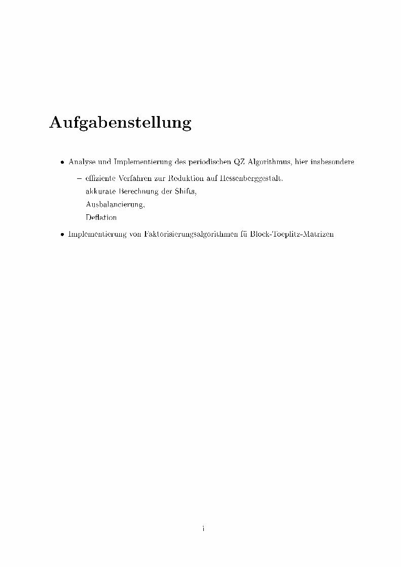
List of Tables1.1 Flop counts for the Hessenberg reduction. . . . . . . . . . . . . . . . . . . 181.2 Execution times for the Hessenberg reduction . . . . . . . . . . . . . . . . 221.3 Execution times for the Hessenberg reduction . . . . . . . . . . . . . . . . 221.4 Execution times for the Hessenberg reduction . . . . . . . . . . . . . . . . 221.5 Flop counts for the de ation of in�nite eigenvalues. . . . . . . . . . . . . . 302.1 Execution times for the Cholesky factorization . . . . . . . . . . . . . . . . 562.2 Summary description of applications. . . . . . . . . . . . . . . . . . . . . . 702.3 Comparative results for computing the QR factorization. . . . . . . . . . . 712.4 Execution times for the QR factorization. . . . . . . . . . . . . . . . . . . . 72
v

vi LIST OF TABLES

List of Figures1.1 Backward errors for the eigenvalue computation of matrix products. . . . . 21.2 Diagrams of the bulge chasing process. . . . . . . . . . . . . . . . . . . . . 262.1 Condition numbers of a block Toeplitz matrix. . . . . . . . . . . . . . . . . 542.2 Cholesky factorization residuals. . . . . . . . . . . . . . . . . . . . . . . . . 552.3 CONVH versus DE01OD. . . . . . . . . . . . . . . . . . . . . . . . . . . . 652.4 Number of multiplications surface plot. . . . . . . . . . . . . . . . . . . . . 672.5 Multiplication versus convolution for point and block Toeplitz matrices. . . 68
vii

viii LIST OF FIGURES

IntroductionStructured matrices are encountered in various application �elds. This work is concernedwith two types of structures.The �rst to mention is the periodic eigenproblem. Depending on the point of viewthis problem can be treated as an ordinary eigenproblem where the involved matrix isrepresented by a product or quotient of several matrices. Or, more appropriate to theusual de�nition of structure, the periodic case can be seen as a generalized eigenproblemwith a special sparsity pattern.Strongly connected to this problem are the linear periodic discrete-time systems. Vari-ous processes in chemical, electrical and aerospace engineering can be modeled using suchperiodic systems. Furthermore, it is the simplest extension of the time-invariant case.In reliable methods for pole placement [61] or state feedback control [60] related toperiodic systems the periodic QZ algorithm often represents the �rst and most expensivestep. This algorithm is also a stable method for �nding eigenvalues and invariant subspacesof periodic eigenproblems [10, 35, 64]. Furthermore, it can be used to solve a broad varietyof matrix equations [16, 62, 67]. Another application arises in the context of Hamiltonianpencils [6].Once the QZ algorithm was established by Moler and Stewart [51], a number of subse-quent publications was concerned with computational and theoretical details re�ning thealgorithm. Particularly mentioned should be the papers of Kaufman and Ward [42, 69, 70].Surprisingly, there do not seem to exist similar works for the periodic QZ algorithm whichcan be considered as a generalization of the QZ algorithm. Some thoughts on the QZ beara trivial extension to the periodic QZ, but phenomena like exponential divergence are notencountered in the �rst case.In Chapter 1 of this thesis methods for order reduction and balancing, blocking tech-niques and special de ation strategies are discussed. This details will not give the periodicQZ a di�erent shape, but it is shown that they may result in a gain of performance andreliability.The second type of structure comes along with Toeplitz matrices, or, more general,with matrices of low displacement rank. The concept of displacement leads to powerfulcharacterizations of a variety of n-by-m matrices whose entries are dependent on as fewas O(n+m) parameters [34, 40]. Although our main interest is focused on block Toeplitzmatrices, Chapter 2 starts with a general treatment of the block displacement concept.This �nally leads to e�cient implementations of the generalized Schur algorithm for solvinglinear equations and least squares problems involving block Toeplitz matrices. Again, thismethods are far from being novel [25, 40]. However, some details like blocking and pivotingtechniques are presented for the �rst time. ix
x INTRODUCTIONPeriodicity and displacement are not unrelated. Both arise from control theory, partic-ularly from linear discrete-time systems. Moreover, block circulant matrices play a role inin Section 1.4 when balancing periodic eigenproblems. Recently, an algebraic link betweenmatrix pencils and block Toeplitz matrices was established [12].I have to say thank you to many friendly and respectful researchers for answering mails,giving useful comments and sending unpublished reports. This list includes Peter Benner,Lars Eld�en, Georg Heinig, John Hench, Linda Kaufman, Bo K�agstr�om, Kurt Lust, KarlaRost, Vasile Sima, Michael Stewart, Paul Van Dooren, Charles Van Loan, Eric Van Vleck,Andras Varga, David Watkins and Honggou Xu.I am much obliged to my advisors, Ralph Byers and Volker Mehrmann, for help, sup-port, travel funds, lots of opportunities and a nice Thanksgiving in Lawrence.
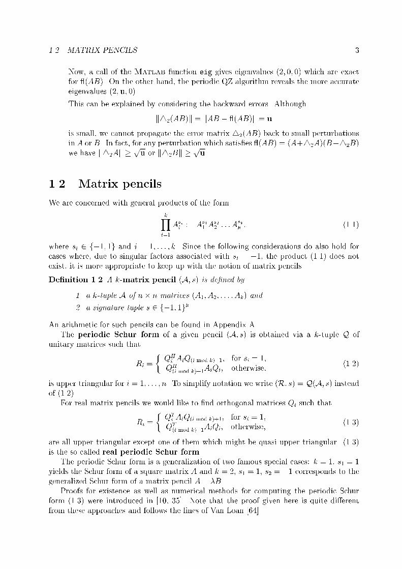
ConventionsWe describe the not explicitly de�ned notation used in this thesis . The following conven-tions are partly taken from [37].Generally, we use capital letters for matrices, subscripted lower case letters for matrixelements, lower case letters for vectors and lower case Greek letters for scalars. The vectorspace of all real m-by-n matrices is denoted by Rm;n and the vector space of real n-vectorsby Rn . For matrix pencils, as de�ned in Chapter 1, Al is the l-th matrix of the pencil andaij:l the (i; j) entry in Al.Algorithms are expressed using a pseudocode based on the Matlab1 language [48].Submatrices are speci�ed with the colon notation as used inMatlab: A(p : q; r : s) denotesthe submatrix of A formed by the intersection of rows p to q and columns r to s. Whendealing with block structures even this convenient notation becomes a mess. For a matrixA with uniquely speci�ed block pattern Ai� denotes the i-th block row, A�j the j-th blockcolumn and Aij the (i; j) block of A.The Kronecker product of two matrices is denoted by . The only nonzero elements ofthe n-by-n matrix diag(a1; : : : ; an) are on its diagonal, given by a1; : : : ; an. The direct sumA� B is a block diagonal matrix with diagonal blocks A and B.We make use of the oor function: bxc is the largest integer less than or equal to x.The elementwise multiplication of two vectors is denoted by x: � y and the elementwisedivision by x:=y.For a matrix A 2 Rm;n , the matrix jAj is equivalent to A only that all elements arereplaced by their absolute values. If not otherwise stated, then kAk denotes the spectralnorm of A, and �(A) = kAk � kAyk the corresponding condition number, where Ay is thegeneralized Moore-Penrose inverse of A.Special symbols:In The identity matrix of order n.�pq Signature matrix, �pq = Ip � (�Iq).0 A zero matrix of appropriate dimension.? An unspeci�ed part of a matrix.ei The i-th unit vector.�ij Kronecker delta, �ij = � 1 if i = j;0 otherwise.�(S) If S is a true-false statement then �(S) = � 1 if S is true,0 if S is false.1Matlab is a registered trademark of The MathWorks, Inc.xi

xii CONVENTIONSThe unit roundo�, which in our computational setting is 2�53, is denoted by u. Thecost of algorithms are measured in ops. A op is an elementary oating point operation:+;�; = or �. Only the highest-order terms of op counts are stated.We were fortunate to have access to the following computing facility:Type Origin 2000Processors 2 � 400 MHz IP27 R12000Memory 16 gigabytesLevel 1 cache 32 kilobytes data and 32 kilobytes instruction cache per processorLevel 2 cache 8 megabytes combined data and instruction cacheAccording to its server name karl.math.ukans.edu, the computer is referred as karl.All Fortran 77 programs were compiled with version 7.30 of the MIPSpro compiler withoptions -n32 -mips4 -r10000 -TARG:madd=ON:platform=ip27 -OPT:Olimit=0 -LNO.The programs call optimized BLAS and LAPACK [2] subroutines from the SGI/CrayScienti�c Library version 1.2.0.0. We observed that the measured execution times of anyparticular program with its particular data might vary by a few percent. Automatic paral-lelization was not used, all programs were serially executed. Some numerical experimentsinvolve Matlab version 5.3 (R11).

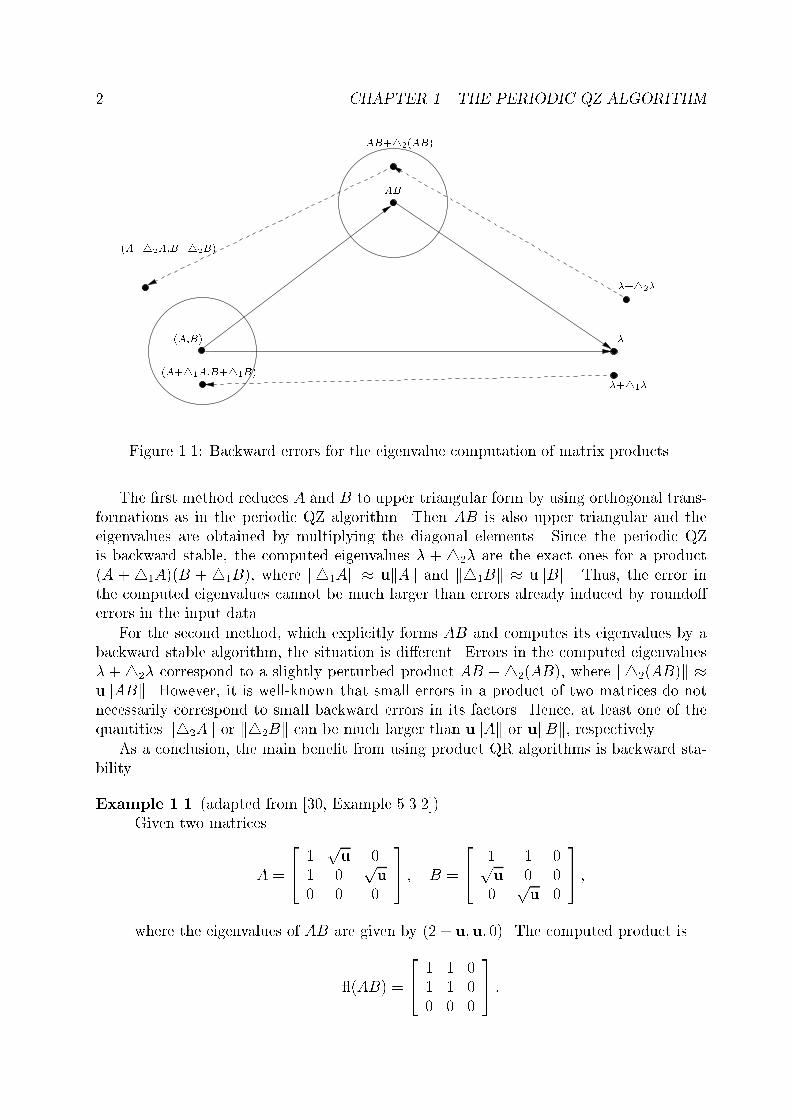
Chapter 1The Periodic QZ Algorithm1.1 IntroductionA brief history of product QR algorithms It was 1965 when Golub and Kahan [29]developed a method for computing the singular value decomposition (SVD) of a matrix A.The algorithm implicitly applies a QR algorithm to ATA working directly on the matrixof A. This approach avoids loss of information implicated by the formation of ATA, whichis a preprocessing step for naive SVD algorithms as described in [30, Section 8.6.2].The generalized eigenproblem is concerned with computing eigenvalues and eigenvectorsof the product AB�1 for some square matrices A and B. The so called QZ algorithmis una�ected by a singular or ill-conditioned B matrix and was invented by Moler andStewart [51] in 1973. Again, the method works directly with the factors A and B ratherthan forming the quotient AB�1 explicitly.Two years later, Van Loan [64] published an algorithm for solving eigenproblems relatedto general products of the form A�1B�1CD, which, of course, does not form the product.Every unitary Hessenberg matrix of order n can be factored into n�1 Givens rotations.A QR algorithm which exclusively involves these factors was presented by Ammar, Graggand Reichel [1] in 1985.Finally, during the years 1992-94, Bojanczyk, Golub and Van Dooren [10] and Henchand Laub [35] independently derived an algorithm for the numerically stable computationof the Schur form of large general products like A1A�12 A3A4A�15 A�16 A7: To the best of ourknowledge, there exist 3 implementations of the so called periodic QZ algorithm, namely:1. the SLICOT [7] subroutines MB03VD and MB03WD dealing with products of the formA1A2A3 : : : Ak; implemented by Varga,2. FORTRAN 77 routines for the same kind of products developed by Lust in thecontext of bifurcation analysis and Floquet multipliers [46],3. the Periodic Schur Reduction Package by Mayo and Quintana [49] for more generalproducts A1A�12 A3A�14 : : : Ak:What is the bene�t from product QR algorithms ? The backward error analysis oftwo di�erent methods for computing the eigenvalues of a matrix product AB is illustratedin Figure 1.1. 1
2 CHAPTER 1. THE PERIODIC QZ ALGORITHM
(A;B) �AB
(A+41A;B+41B)
AB+42(AB)
�+41��+42�(A+42A;B+42B)
Figure 1.1: Backward errors for the eigenvalue computation of matrix products.The �rst method reduces A and B to upper triangular form by using orthogonal trans-formations as in the periodic QZ algorithm. Then AB is also upper triangular and theeigenvalues are obtained by multiplying the diagonal elements. Since the periodic QZis backward stable, the computed eigenvalues � + 42� are the exact ones for a product(A +41A)(B +41B), where k41Ak � ukAk and k41Bk � ukBk. Thus, the error inthe computed eigenvalues cannot be much larger than errors already induced by roundo�errors in the input data.For the second method, which explicitly forms AB and computes its eigenvalues by abackward stable algorithm, the situation is di�erent. Errors in the computed eigenvalues� +42� correspond to a slightly perturbed product AB +42(AB), where k42(AB)k �ukABk. However, it is well-known that small errors in a product of two matrices do notnecessarily correspond to small backward errors in its factors. Hence, at least one of thequantities k42Ak or k42Bk can be much larger than ukAk or ukBk, respectively.As a conclusion, the main bene�t from using product QR algorithms is backward sta-bility.Example 1.1 (adapted from [30, Example 5.3.2])Given two matricesA = 24 1 pu 01 0 pu0 0 0 35 ; B = 24 1 1 0pu 0 00 pu 0 35 ;where the eigenvalues of AB are given by (2 + u;u; 0). The computed product is (AB) = 24 1 1 01 1 00 0 0 35 :
1.2. MATRIX PENCILS 3Now, a call of the Matlab function eig gives eigenvalues (2; 0; 0) which are exactfor (AB). On the other hand, the periodic QZ algorithm reveals the more accurateeigenvalues (2;u; 0).This can be explained by considering the backward errors. Althoughk42(AB)k = kAB � (AB)k = uis small, we cannot propagate the error matrix 42(AB) back to small perturbationsin A or B. In fact, for any perturbation which satis�es (AB) = (A+42A)(B+42B)we have k42Ak � pu or k42Bk � pu.1.2 Matrix pencilsWe are concerned with general products of the formkYi=1 Asii := As11 As22 : : : Askk ; (1.1)where si 2 f�1; 1g and i = 1; : : : ; k. Since the following considerations do also hold forcases where, due to singular factors associated with si = �1, the product (1.1) does notexist, it is more appropriate to keep up with the notion of matrix pencils.De�nition 1.2 A k-matrix pencil (A; s) is de�ned by1. a k-tuple A of n� n matrices (A1; A2; : : : ; Ak) and2. a signature tuple s 2 f�1; 1gk.An arithmetic for such pencils can be found in Appendix A.The periodic Schur form of a given pencil (A; s) is obtained via a k-tuple Q ofunitary matrices such thatRi = � QHi AiQ(i mod k)+1; for si = 1;QH(i mod k)+1AiQi; otherwise; (1.2)is upper triangular for i = 1; : : : ; n. To simplify notation we write (R; s) = Q(A; s) insteadof (1.2).For real matrix pencils we would like to �nd orthogonal matrices Qi such thatRi = � QTi AiQ(i mod k)+1; for si = 1;QT(i mod k)+1AiQi; otherwise; (1.3)are all upper triangular except one of them which might be quasi upper triangular. (1.3)is the so called real periodic Schur form.The periodic Schur form is a generalization of two famous special cases: k = 1, s1 = 1yields the Schur form of a square matrix A and k = 2, s1 = 1, s2 = �1 corresponds to thegeneralized Schur form of a matrix pencil A� �B.Proofs for existence as well as numerical methods for computing the periodic Schurform (1.3) were introduced in [10, 35]. Note that the proof given here is quite di�erentfrom these approaches and follows the lines of Van Loan [64].

4 CHAPTER 1. THE PERIODIC QZ ALGORITHMTheorem 1.3 For every k-matrix pencil (A; s) there exists a k-tuple Q of unitary matricessuch that Q(A; s) is in periodic Schur form (1.2).Proof: First assume that allAi, i = 1; : : : ; k are invertible. By the Schur decomposition[30, Theorem 7.1.3] there exists a unitary matrix Q1 such thatR = QH1 kYi=1 Asii !Q1is upper triangular. Now, after application of the procedurefor i = k : �1 : 2 doApply a QR/RQ factorization such that Ai = � QiRi; si = 1;RiQHi ; si = �1: :Update Ai�1 = � Ai�1Qi si�1 = 1;QHi Ai�1 si�1 = �1: :endwe have de�ned all necessary Qi of a unitary k-tuple Q. Setting (R; s) = Q(A; s)the above procedure provides upper triangular Ri for i = 2; : : : ; k. Note that R1 canbe written as a product of upper triangular matrices, namelyR1 = RR�skk R�sk�1k�1 : : : R�s22 :We have thus proved the decomposition in the case when our pencil consists ofnonsingular matrices. We can nevertheless proceed without this restriction. Forgeneral (A; s) let Ai = UiSi, i = 1; : : : ; k, be the QR factorization of Ai where Si hasnonnegative diagonal elements. IfA[m]i = Ui�Si + 1mIn�then it follows that kA[m]i � Aik ! 0 for m!1 and that for every positive integerm, rank A[m]i = n. Let us de�neA[m] = fA[m]1 ; A[m]2 ; : : : ; A[m]k g;then by the �rst part of the proof, we can �nd unitary k-tuples Q[m] such that eachpencil Q[m](A[m]; s) consists of upper triangular matrices. Using a C n2 version of theBolzano-Weierstrass theorem (see [73, p. 105]) repeatedly, we �nd a subsequencefmig of the positive integers such that Q[mi] converges to a unitary k-tuple Q. Thisconstruction enforces the subdiagonal entries of Q(A; s) to be zero.Remark 1.4 For our further considerations we will sometimes assume that s1 = 1. Thisis justi�ed by the following observation.If there exists an index j such that sj = 1 then we may consider the reorderd pencil(A(j); s(j)) with A(j) = (Aj; Aj+1; : : : ; Ak; A1; : : : ; Aj�1) (1.4)
1.2. MATRIX PENCILS 5and s(j) = (sj; sj+1; : : : ; sk; s1; : : : ; sj�1): (1.5)Since (Q(A; s))(j) = Q(j)(A(j); s(j)), the periodic Schur decomposition of (A(j); s(j))also supplies that one of (A; s), and vice versa.In the case of s = (�1;�1; : : : ;�1) we consider the pencil (A(�1); s(�1)) withA(�1) = (Ak; Ak�1; : : : ; A1) and s(�1) = (1; 1; : : : ; 1):Now, we get the Schur form of (A; s) by the identity(Q(A; s))�1 = Q(�k)(A(�1); s(�1));where Q(�k) = (Q(�1))(k).As already seen in the proof of Theorem 1.3 there is a close relationship between theSchur form of general products of matrices and the periodic Schur form.Lemma 1.5 Let (A; s) be a k-matrix pencil and Q unitary such that Q(A; s) is in periodicSchur form. Under the assumption that each Ai with si = �1 is nonsingular, all thefollowing products are in upper triangular formQHj Asjj Asj+1j+1 : : : Askk As11 : : : Asj�1j�1 Qj; j = 1; : : : ; k: (1.6)Proof: The term (1.6) is equivalent toQHj Asjj Qj+1QHj+1Asj+1j+1Qj+2 : : : QHk Askk Q1QH1 As11 Q2 : : : QHj�1Asj�1j�1 Qj j = 1; : : : ; k:From (1.2) we know that this is nothing but a product of upper triangular matrices.However, in general the converse of Lemma 1.5 is not true. Since the diagonal elementsof (1.6) are invariant under commutation all products must have the same eigenvalues.But only under the assumption that these values are distinct and appear in the same orderon the diagonal of (1.6) the uniqueness of the Schur form and Lemma 1.5 guarantee thatQ(A; s) is in periodic Schur form.The following de�nition of eigenvalues is chosen in a way so that if the associatedproduct does exist then its eigenvalues are equivalent to those of the matrix pencil.De�nition 1.6 Let (R; s) = Q(A; s) be in periodic Schur form. If there is no integer jsuch that the product Qki=1 rsijj; i becomes unde�ned we call (A; s) regular and other-wise singular. For a regular pencil and an integer j,1. if all rjj; i corresponding to si = �1 are nonzero we call �j =Qki=1 rsijj; i a �niteeigenvalue of (A; s), and2. if some rjj; i corresponding to si = �1 is zero then (A; s) has an in�nite eigen-value �j =1.

6 CHAPTER 1. THE PERIODIC QZ ALGORITHMSingular pencils are most often pathological cases. The following example shows that inthese cases the periodic Schur decomposition does not yield a proper de�nition of eigen-values.Example 1.7 Let (A; s) = ��� 2 10 0 � ; � 0:5 10 0 �� ; f1;�1g�in periodic Schur form with eigenvalues (4; 0=0). By permutations, (A; s) becomes(A0; s) = ��� 1 20 0 � ; � 1 0:50 0 �� ; f1;�1g� ;where the eigenvalues are given by (1; 0=0).Hence, we need to separate the singular and the regular parts beforehand. Recently,techniques were developed to achieve this goal by reducing the matrix pencil to blockdiagonal form [44].The eigenvalues of products or quotients of two symmetric positive de�nite matricesare always real and positive [30, Section 8.7]. Another example shows that this propertygets lost for larger products.Example 1.8 Consider the 3-matrix pencil(A; s) = ��� 13 �16�16 20 � ; � 5 �2�2 1 � ; � 4 00 1 �� ; f1;�1; 1g� :The orthogonal tupleQ = �15 � �3 �44 �3 � ; 1p2 � 1 �11 1 � ; 1p10 � �3 �11 �3 ��transforms (A; s) to periodic Schur form,Q(A; s) = � 15p2 � 25 2310 8 � ; 1p5 � �5 120 �1 � ; 1p10 � 8 90 5 �� :Hence, the eigenvalues of (A; s) are both �4. Note that all matrices of the pencil aresymmetric positive de�nite.We can introduce a norm on k-matrix tuples viakAk = maxj=1;:::;k kAjk; (1.7)where kAjk can denote one of your favorite unitarily invariant matrix norm like k � k2 ork � kF . As in the matrix case orthogonal transformations do not alter the tuple norm,in particular we have for an orthogonal (resp. unitary) tuple Q that kRk = kAk where(R; s) = Q(A; s). Furthermore, continuity of eigenvalues may be extended to matrixtuples.

1.2. MATRIX PENCILS 7Lemma 1.9 For a sequence of k-matrix pencils (Ai; s) let (Ai; s)! (A; s) where (A; s) isregular. Then the eigenvalues of (Ai; s) converge to those of (A; s).Proof: By Theorem 1.3 we can assume that (A; s) is in upper triangular form. Usingthe Frobenius norm yields for the diagonal entries of (Ai; s) that there exist complexnumbers rjj:l so that r(i)jj:l ! rjj:l; l = 1; : : : ; k;where r(i)jj:l is the (j; j)-entry in the l-th matrix of the pencil (Ai; s). Thus, the entriesin the strictly lower triangular parts of (Ai; s) will certainly converge to zero. Now,the regularity of (A; s) implies�r(i)jj:1�s1 �r(i)jj:2�s2 : : :�r(i)jj:k�sk ! �j;where �j denotes the j-th eigenvalue of (A; s).Remark 1.10 Note that Lemma 1.9 does not hold for singular pencils. E.g., consider thesequence (Aj; s) = ��� 1=j 00 1 � � 1=j 00 1 �� ; f1;�1g�which converges to a singular pencil. However, the eigenvalues of (Aj; s) obviouslyconverge to f1; 1g.The periodic eigenvalue problem may also be studied via an in ated generalized eigen-value problem [45, 44]. Let us considerB � �C = 26664 B1 B2 . . . Bk37775� �26664 C1C2 . . . Ck
37775 ; (1.8)where (Bi; Ci) = � (In; Ai); if si = 1;(Ai; In); if si = �1:The 2k-matrix pencil(Z; sZ) = (fB;C; : : : ; B; C| {z }k times g; f�1; 1; : : : ;�1; 1g)may be reformulated as a block matrix with k-matrix pencils as entries, namely26664 (A(1); s(1)) (A(2); s(2)) . . . (A(k); s(k)) 37775 ;where the pencils (A(j); s(j)) are as de�ned in Remark 1.4. Hence, we get the followingresult.

8 CHAPTER 1. THE PERIODIC QZ ALGORITHMCorollary 1.11 [45] Let (A; s) be a regular k-matrix pencil of n � n matrices with reigenvalues. Then the generalized eigenvalue problem B��C as de�ned in (1.8) hasrk eigenvalues �ij where i = 1; : : : ; r and j = 1; : : : ; k so that1. �ij are the k-th roots of �i if �i is �nite, and2. �ij =1 if �i =1.The LAPACK implementations of the QR and QZ algorithms are preceded by permu-tations to eventually isolate eigenvalues and (optionally) by diagonal similarity transforma-tions to make the rows and columns of the involved matrices as close in norm as possible.While the �rst enhances e�ciency for certain matrices, the latter attempts to improve therelative accuracy of the computed eigenvalues. The generalization to periodic eigenvalueproblems is presented in a style close to the paper of Ward [70].1.3 Order ReductionFor some factors A1; A2; : : : ; Ak it is possible to reduce the problem of computing theperiodic Schur form (1.2) by solely using row and column permutations.That is, determine permutation matrices P1; P2; : : : ; Pk such thatP1As11 P T2 = 24 A11; 1 A12; 1 A13; 10 A22; 1 A23; 10 0 A33; 1 35s1P2As22 P T3 = 24 A11; 2 A12; 2 A13; 20 A22; 2 A23; 20 0 A33; 2 35s2 (1.9)...PkAskk P T1 = 24 A11; k A12; k A13; k0 A22; k A23; k0 0 A33; k 35sk ;where A11; i and A33; i are upper triangular matrices for i = 1; : : : ; k. Now, the computa-tional part of the reduction to periodic Schur form can be restricted to the subpencil inthe middle, (A22; s) = (fA22; 1; : : : ; A22; kg; s):First, we want to limit the variety of signatures arrays. By introducing identities,it can be assumed that each signature si = �1 is proceeded by si+1 = 1. For a pairfsi; si+1g = f�1; 1g, the matrices PiAiP Ti+1 and PiAi+1P Ti+1 are in upper block triangularform (1.9) if and only if Pi(jAij+ jAi+1j)P Ti+1 is in upper block triangular form. Hence, wecan assume w.l.o.g. that s = (1; : : : ; 1).For k = 2, the existence of two permutation matrices P1 and P3 such that P1jA1jjA2jP T3is block upper triangular is a necessary but not su�cient condition for the existence of apermutation matrix P2 such that P1A1P T2 and P2A2P T3 are both block upper triangular.This fact can be used for the order reduction algorithm.

1.3. ORDER REDUCTION 9Let Bi be de�ned as Bi = jA1jjA2j : : : jAij; i = 1; : : : ; k;then the following order reduction algorithm is proposed:1. Find all possible integers p(1)j , j = 1; : : : ; l, such that, after a swap of rows p(1)j $ nand columns p(1)j $ n (from now on denoted by (p(1)j ; p(1)j )) , the last row of Bk hasonly one nonzero element at the n-th position.2. For each p(1)j the possibility to reveal such a row in the updated factors Bk�1 andAk is tested. For example the product P1BkP T1 = (P1Bk�1)(jAkjP T1 ) could have theform 2664 � � � �� � � �� � � �0 0 0 0 3775 = 2664 � � � �� � � �� � � �0 0 0 0 37752664 � � � �� � � �� � � �� � � � 3775or 2664 � � � �� � � �� � � �0 0 0 � 3775 = 2664 � � � �� � � �� � � �0 � 0 0 37752664 � � � �0 0 0 �� � � �� � � � 3775 :In the �rst case there does not exist an inner permutation which annihilates the lastrows of Bk�1 and Ak besides the (n; n) element. However, in the latter there existssuch a permutation, namely p(k)1 = 3. In the matrix product2664 � � � �� � � �� � � �0 0 0 0 3775 = 2664 � � � �� � � �� � � �0 0 0 0 37752664 0 0 0 �� � � �0 0 0 �� � � � 3775 ;we encounter p(k)1 = 1 and p(k)2 = 3 as possible inner permutations.In general, each p(1)j corresponds to a set Sj = fp(k)i j i = 1; : : : ; ljg of suitable innerswaps, that is, for the corresponding permutation matrices P1 and Pk, the �rst n� 1entries in the last rows of the matrices P1Bk�1P Tk and PkAkP T1 are zero.3. This gives us for each p(1)j exactly card(Sj) di�erent inner permutations. IflXj=1 card(Sj) = 0;then the matrix pencil cannot be reduced. Otherwise the same test is applied to theproduct Bk�2 � jAk�1j, now for the at most n2 di�erent row/column swaps�p(1)j ; p(k)i � ; p(k)i 2 Sj; j = 1; : : : ; l:

10 CHAPTER 1. THE PERIODIC QZ ALGORITHM4. This procedure is recursively applied to the productsBk�3 � jAk�2j; Bk�4 � jAk�3j; : : : :If there is a suitable inner perturbations for the last product jA1j � jA2j, then wesucceeded in reducing the order by one, that is, the permuted product will look like2664 � � � �� � � �� � � �0 0 0 � 37752664 � � � �� � � �� � � �0 0 0 � 3775 : : :2664 � � � �� � � �� � � �0 0 0 � 3775 : (1.10)Note that the complexity of the tests will not explode; the cardinality of outer row /column swaps is bounded by n2. If the tests are e�ciently implemented, we get an overallcomplexity of at most O(kn2), which is low in comparison with the bene�ts from an orderreduction.Example 1.12 LetA1 = 2664 1 0 0 00 0 0 00 0 0 11 0 0 0 3775 ; A2 = 2664 1 0 0 10 1 1 00 0 0 11 0 0 0 3775 ; A3 = 2664 1 0 0 01 0 0 00 0 0 00 0 0 0 3775 ;then B2 = 2664 1 0 0 10 0 0 01 0 0 01 0 0 1 3775 ; B3 = 2664 1 0 0 00 0 0 01 0 0 01 0 0 0 3775 :Possible outer permutations are p(1)1 = 1 and p(1)2 = 2. The corresponding sets ofinner permutations for the product B2 � jA3j are given by S1 = f;g and S2 = f3; 4g:The permuted factors of jA1j � jA2j for each of the 2 possible row/column swaps areshown below. (2; 3) : 2664 1 0 0 01 0 0 00 0 0 10 0 0 0 3775 � 2664 1 0 1 00 1 0 10 0 1 01 0 0 0 3775(2; 4) : 2664 1 0 0 01 0 0 00 0 0 10 0 0 0 3775 � 2664 1 0 0 10 1 1 00 0 0 11 0 0 0 3775Only for the row/column swap (2; 4) it is possible to �nd an inner permutation,namely 3$ 4.

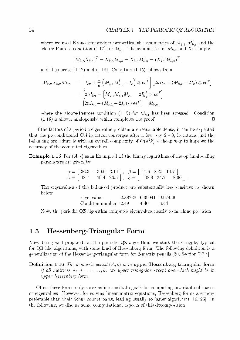
1.4. BALANCING 11Hence, by swapping rows 2$ 4, columns 3$ 4 of A1, rows 3$ 4 of A2 and columns2$ 4 of A1, we have derived the reduced problemA1 = 2664 1 0 0 01 0 0 00 0 1 00 0 0 0 3775 ; A2 = 2664 1 0 0 10 1 1 01 0 0 00 0 0 1 3775 ; A3 = 2664 1 0 0 01 0 0 00 0 0 00 0 0 0 3775 :After having reduced the problem dimension by one, we can repeat the algorithm forthe north west blocks in (1.10), which �nally yields the blocks A33; 1; A33; 2; : : : ; A33; k in(1.9).The A11; 1; A11; 2; : : : ; A11; k blocks are obtained by the same method only that we now(implicitly) consider the pencil�fPATkP; PATk�1P; : : : ; PAT1 Pg; f1; : : : ; 1g�where P is the identity matrix, ipped from the left to the right.1.4 BalancingAs a rule of thumb we haveForward error = Condition number � Backward error:Thus, in order to obtain accurate eigenvalues, the backward error of the implementedmethod as well as the conditioning of the problem must be small. The aim of this sectionis not to reduce the backward error (the periodic QZ algorithm is already backward stable)but the condition numbers of the eigenvalues. Such condition numbers can be foundin [8, 45].Example 1.13 Consider the matrix pencil (A; s) = (fA1; A2; A3; A4g; f1;�1; 1;�1g) withA1 = 24 5�26 3�14 6�166�06 2+06 3+044�16 2�04 5�06 35 ; A2 = 24 6�28 3�16 5�187�09 3+03 7+016�23 3�11 3�13 35 ;A3 = 24 8�02 6�24 6�115+17 5�05 6+083+03 4�19 7�06 35 ; A4 = 24 9+00 4�22 3�097+20 2�02 9+114+10 6�12 7+01 35�1 ;where the signed integer superscript at the end of a number represents its decimalexponent. Eigenvalues and associated condition numbers are tabulated below.Eigenvalue 2:88728 0:39941 0:07459Conditon number 4:32� 1021 1:77� 1021 2:59� 1021Not surprisingly, the periodic QZ algorithm completely fails to reveal any relevantinformation about the eigenvalues.

12 CHAPTER 1. THE PERIODIC QZ ALGORITHMIll-conditioning, caused from matrix entries of widely varying magnitudes, can be re-moved by a preceding balancing step. For positive de�nite diagonal matrices D�, D�, D ,D� the eigenvalues of the matrix pencils(fA;B;C;Eg; s) ; s = f1;�1; 1;�1g;and (fD�AD�; D BD�; D CD�; D�ED�g; s) (1.11)are equivalent. Di�erent sign patterns do not pose a problem; if for example s2 = 1, thenin the following discussion B can virtually be replaced by the matrix~B = �~bij�ni;j=1 := ��(bji 6= 0) � 1bji�ni;j=1 ;where for 0 �1 situations the formal term �(bji 6= 0)=bji is de�ned to be zero. The diagonaltransformations should reduce the condition numbers and thus improve the accuracy ofthe computed eigenvalues. However, minimizing the conditioning of the periodic eigenvalueproblem is certainly an unrealistic goal. On the other hand, reducing the magnitude rangesof the elements in the factors seems to be reasonable.Analogously to the generalized eigenvalue problem [70], the balancing step can be for-mulated as the solution of an optimization problem. Let �i, �i, i and �i denote the binarylogarithms of the i-th diagonal entries in the corresponding diagonal matrices. Then onewants to minimize the expressionS(�; �; ; �) = Pni;j=1 (�i + �j + log2 jaijj)2 + ( i + �j + log2 jbijj)2 (1.12)+( i + �j + log2 jcijj)2 + (�i + �j + log2 jeijj)2:By di�erentiation an optimal point (�; �; ; �) satis�es the linear system of equations2664 F (E;A) H(A) 0 H(E)HT (A) G(A;B) HT (B) 00 H(B) F (B;C) H(C)HT (E) 0 HT (C) G(C;E) 37752664 �� � 3775 = �2664 row(A) + row(E)col(B) + col(A)row(C) + row(B)col(E) + col(C) 3775 ; (1.13)where the notation is as follows:1. F (X; Y ) (resp. G(X; Y )) is a diagonal matrix whose elements are given by thenumber of nonzero entries in the rows (resp. columns) of X and Y ,2. H(X) is the incidence matrix of X,3. row(X) (resp. col(X)) is the vector of row (resp. column) sums of the matrix��(xij 6= 0) � log2 jxijj�ni;j=1:

1.4. BALANCING 13It can be shown that the linear system (1.13) is symmetric, positive semide�nite andconsistent. However, the system is of order kn. Thus, a solution via an SVD or rankrevealing QR factorization requires O(k3n3) ops which is unacceptably high in comparisonwith the periodic QZ algorithm which only requires O(kn3) ops.We rather propose to use a generalized conjugate gradient (CG) iteration as in [70]. Inthe following discussion we drop the assumption k = 4 and consider pencils of arbitrarylength k > 2. To reduce the number of iterations in the CG it is crucial to �nd a suitablepreconditioner. For this purpose we assume that all the matrices in (A; s) are completelydense. Then the system matrix in (1.13) is given byMk;n = �2nIkn + (Mk;1 � 2Ik) eeT � ; (1.14)where Mk;1 is, for even k, the k-by-k circulant matrix with �rst row [ 2 1 0 : : : 0 1 ],or, for odd k, the skew circulant matrix with �rst row [ 2 1 0 : : : 0 � 1 ] and e is then-vector of all ones.To be successful as a preconditioner, the application of the Moore-Penrose generalizedinverse M yk;n to a vector should not be expensive. Indeed, for x 2 Rk the product M yk;1xcan be formed within O(k) operations by using an incomplete Cholesky factorization whichexploits the underlying sparsity structure.The following lemma shows that forming M yk;nx for x 2 Rkn only requires O(kn) ops.Lemma 1.14 The Moore-Penrose generalized inverse of the matrix Mk;n as de�ned in(1.14) is given by Xk;n = 1n2 �n2 Ikn + �M yk;1 � 12Ikn� eeT� :Proof: We prove that Xk;n satis�es the four Moore-Penrose conditionsMk;nXk;nMk;n =Mk;n; (1.15)Xk;nMk;nXk;n = Xk;n; (1.16)(Mk;nXk;n)T =Mk;nXk;n; (1.17)(Xk;nMk;n)T = Xk;nMk;n: (1.18)Then it readily follows that Xk;n =M yk;n [30, Section 5.5.4].We have Mk;nXk;n = �Ikn + 1n �2M yk;1 + 12Mk;1 � 2Ik eeT�+ 1n2 (Mk;1 � 2I)�M yk;1 � 12Ik� e(eT e)eT�= Ikn + 1n �Mk;1M yk;1 � Ik� eeT ;and analogously,Xk;nMk;n = Ikn + 1n �M yk;1Mk;1 � Ik� eeT= Ikn + 1n �Mk;1M yk;1 � Ik� eeT =Mk;nXk;n;
14 CHAPTER 1. THE PERIODIC QZ ALGORITHMwhere we used Kronecker product properties, the symmetries of Mk;1;M yk;1 and theMoore-Penrose condition (1.17) for Mk;1. The symmetries of Mk;n and Xk;n imply(Mk;nXk;n)T = Xk;nMk;n = Xk;nMk;n = (Xk;nMk;n)T ;and thus prove (1.17) and (1.18). Condition (1.15) follows fromMk;nXk;nMk;n = �Ikn + 1n �Mk;1M yk;1 � Ik� eeT� �2nIkn + (Mk;1 � 2Ik) eeT �= h2nIkn + �Mk;1M yk;1Mk;1 � 2Ik� eeT i= �2nIkn + (Mk;1 � 2Ik) eeT � =Mk;n;where the Moore-Penrose condition (1.15) for Mk;1 has been stressed. Condition(1.16) is shown analogously, which completes the proof.If the factors of a periodic eigenvalue problem are reasonable dense, it can be expectedthat the preconditioned CG iteration converges after a few, say 2 - 3, iterations and thebalancing procedure is with an overall complexity of O(n2k) a cheap way to improve theaccuracy of the computed eigenvalues.Example 1.15 For (A; s) as in Example 1.13 the binary logarithms of the optimal scalingparameters are given by� = � 36:3 �30:0 3:14 � ; � = � 47:6 8:85 14:7 � = � 42:7 �20:4 26:5 � ; � = � �38:8 34:7 �8:96 � :The eigenvalues of the balanced product are substantially less sensitive as shownbelow. Eigenvalue 2:88728 0:39941 0:07459Conditon number 2:49 4:40 3:44Now, the periodic QZ algorithm computes eigenvalues nearly to machine precision.1.5 Hessenberg-Triangular FormNow, being well prepared for the periodic QZ algorithm, we start the struggle, typicalfor QR like algorithms, with some kind of Hessenberg form. The following de�nition is ageneralization of the Hessenberg-triangular form for 2-matrix pencils [30, Section 7.7.4].De�nition 1.16 The k-matrix pencil (A; s) is in upper Hessenberg-triangular formif all matrices Ai, i = 1; : : : ; k, are upper triangular except one which might be inupper Hessenberg form.Often these forms only serve as intermediate goals for computing invariant subspacesor eigenvalues. However, for solving linear matrix equations, Hessenberg forms are morepreferable than their Schur counterparts, leading usually to faster algorithms [16, 26]. Inthe following, we discuss some computational aspects of this decomposition.

1.5. HESSENBERG-TRIANGULAR FORM 151.5.1 Unblocked ReductionWe present 2 di�erent algorithms to compute the periodic upper Hessenberg form. Algo-rithm 1.17 is a generalization of the 2-matrix pencil case [30, Algorithm 7.7.1]. Algorithm1.18 is a combination of two algorithms proposed in [10].Algorithm 1.17 Given a k-matrix pencil (A; s) with Ai 2 Rn�n (resp. C n�n) and s1 =1, the following algorithm overwrites A with an periodic upper Hessenberg pencilQ(A; s) where Qi is orthogonal (resp. unitary) for i = 1; : : : ; k.% Step 1: Transform (A2; : : : ; Ak) to upper triangular formfor i = k : �1 : 2 doApply a QR/RQ factorization such that Ai = � QiRi; si = 1RiQHi ; si = �1 :Update Ai = Ri and Ai�1 = � Ai�1Qi si�1 = 1QHi Ai�1 si�1 = �1 :end% Step 2: Transform A1 to upper Hessenberg formfor j = 1 : n� 2 dofor l = n : �1 : j + 2 do[c; s] = givens(A1(l � 1; j); A1(l; j))A1(l � 1 : l; j : n) = � c1 s1��s1 c1 �H A1(l � 1 : l; j : n)Propagate the rotation successively through Ak; Ak�1; : : : ; A2.A1(1 : n; l � 1 : l) = A1(1 : n; l � 1 : l) � c2 s2��s2 c2 �endendThe main computational burden in Step 2 of Algorithm 1.17 is the application ofGivens rotations. This might not always be favorable, especially if the pencil contains longsubproducts with signature (1; : : : ; 1). It is possible to replace rotations by Householdertransformations for a certain subset S � f1; : : : ; kg which is de�ned asS = fl 2 [1; : : : ; k] : sl = 1g (1.19)Note that the following algorithm does also work with each subset of S which contains 1.Furthermore it reduces to Algorithm 1.17 if S = f1g.Algorithm 1.18 Given a k-matrix pencil (A; s) with Ai 2 Rn�n (resp. C n�n) and s1 =1, the following algorithm overwrites A with an periodic upper Hessenberg pencilQ(A; s) where Qi is orthogonal (resp. unitary) for i = 1; : : : ; k.1. Choose S as in (1.19) and let smax = maxfk 2 Sg.2. Transform all matrices Ak with k 62 S to upper triangular form.

16 CHAPTER 1. THE PERIODIC QZ ALGORITHM3. Transform the remaining matrices to upper triangular resp. upper Hessenbergform:for j = 1 : n� 1 dofor l = smax : �1 : 2 doif l 2 S thenAnnihilate Al(j + 1 : n; j) by 8<: Householderre ections if l � 1; l 2 S;Givens rotations otherwise.Apply last transformation to Al�1.elseAl is already upper triangular, push the Givens rotations throughAl as in Step 2 of Algorithm 1.17.endendAnnihilate A1(j + 2 : n; j) by � Householder re ections if k = smax;Givens rotations if k 6= smax:for l = k : �1 : smax � 1 doAl is already upper triangular, push the Givens rotations throughAl as in Step 2 of Algorithm 1.17.endApply last transformation to Asmax.endExample 1.19 Let us demonstrate Algorithm 1.18 for a matrix pencil with n = k = 4and s = (1;�1; 1; 1).The �rst step is to transform A2 to upper triangular form which alters A1:2664 � � � �� � � �� � � �� � � � 37752664 � � � �0 � � �0 0 � �0 0 0 � 3775�1 2664 � � � �� � � �� � � �� � � � 37752664 � � � �� � � �� � � �� � � � 3775Now, we choose a Householder re ection from the left to annihilate A4(2 : 4; 1) whichrecombines all columns of A3:2664 � � � �� � � �� � � �� � � � 37752664 � � � �0 � � �0 0 � �0 0 0 � 3775�1 2664 � � � �� � � �� � � �� � � � 37752664 � � � �0 � � �0 � � �0 � � � 3775We cannot apply the same procedure to A3 as long as we want to preserve thetriangular shape of A2. Using a Givens rotation to annihilate the (4; 1)-element inA3 and propagating this transformation over A2 to A1 yields the following diagram:2664 � � � �� � � �� � � �� � � � 3775 x2664 � � � �0 � � �0 0 � �0 0 � � 3775�1 x2664 � � � �� � � �� � � �0 � � � 37752664 � � � �0 � � �0 � � �0 � � � 3775

1.5. HESSENBERG-TRIANGULAR FORM 17x x2664 � � � �� � � �� � � �� � � � 37752664 � � � �0 � � �0 0 � �0 0 0 � 3775�1 2664 � � � �� � � �� � � �0 � � � 37752664 � � � �0 � � �0 � � �0 � � � 3775Continuing this process for the elements (3; 1) and (2; 1) gives:2664 � � � �� � � �� � � �� � � � 37752664 � � � �0 � � �0 0 � �0 0 0 � 3775�1 2664 � � � �0 � � �0 � � �0 � � � 37752664 � � � �0 � � �0 � � �0 � � � 3775Again, we are allowed to use a re ection from the left to zero A1(3 : 4; 1). Note thatthe corresponding transformation on A4 does not destroy the zero structure:2664 � � � �� � � �0 � � �0 � � � 37752664 � � � �0 � � �0 0 � �0 0 0 � 3775�1 2664 � � � �0 � � �0 � � �0 � � � 37752664 � � � �0 � � �0 � � �0 � � � 3775Applying this algorithm to the submatrices Ai(2 : 4; 2 : 4) and Ai(3 : 4; 3 : 4) �nallyyields:2664 � � � �� � � �0 � � �0 0 � � 37752664 � � � �0 � � �0 0 � �0 0 0 � 3775�1 2664 � � � �0 � � �0 0 � �0 0 0 � 37752664 � � � �0 � � �0 0 � �0 0 0 � 3775Flop Count The number of ops needed by Algorithm 1.18 depends on the structureof the signature array s. Alternating signature arrays like (1;�1; 1;�1; : : : ; 1;�1) need alot of Givens rotations while the Hessenberg form of pencils with s = (1; 1; : : : ; 1) may becomputed with the exclusive usage of Householder re ections. In Table 1.1 we list opcounts for 3 di�erently structured signature arrays:s(1) = (1; : : : ; 1| {z }k times )s(2) = (1;�1; : : : ; 1;�1| {z }k=2 times )s(3) = (1; : : : ; 1| {z }k+ times ;�1; : : : ;�1| {z }k� times )Note that the e�ciency of Algorithm 1.17 does not depend on the structure of theunderlying signature array. However, Table 1.1 tells us that the costs of this algorithm arealways greater or equal than those of Algorithm 1.18. Reality, i.e. execution time, mighttell a di�erent story though. This topic is discussed in Section 1.5.4.

18 CHAPTER 1. THE PERIODIC QZ ALGORITHMs # ops # opsAlgorithm 1.17 without Q Accumalation of Qs(1) 193 kn3 � 43n3 133 kn3 � 73n3s(2) 193 kn3 � 43n3 133 kn3 � 73n3s(3) 193 (k+ + k�)n3 � 43n3 133 (k+ + k�)n3 � 73n3Algorithm 1.18 without Q Accumalation of Qs(1) 103 kn3 43kn3s(2) 173 kn3 196 kn3s(3) 103 k+n3 + 193 k�n3 + 53n3 43k+n3 + 133 k�n3 + 23Table 1.1: Flop counts for reducing a k-matrix pencil of n-by-n matrices to Hessenberg-triangular form.1.5.2 Blocked Reduction to Upper r-Hessenberg-Triangular FormBased on the algorithms for the reduction to upper r-Hessenberg-triangular form of 2-matrix pencils by Dackland and K�agstr�om [21] it is quite straightforward to formulateblocked versions of the periodic Hessenberg reduction. Introducing matrix-matrix oper-ations in Step 3 of Algorithm 1.18 allows us the e�cient usage of level-3 BLAS in theupdates of Ai and, if requested, also in the transformation matrices Qi. Roughly speaking,bunches of Givens rotators are replaced by QR factorizations of 2r-by-r matrices resp. RQfactorizations of r-by-2r matrices where r denotes the block size. All occuring Householderre ections are blocked. That is, we take a product of r Householder matrices,Q = (I + �1v1vT1 )(I + �2v2vT2 ) : : : (I + �rvrvTr );and represent them as one rank-r update. For this purpose, two matrices W;Y 2 Rn;r areconstructed so that Q = I +WY T [30, Algorithm 5.1.2]. The application of Q to a matrixC 2 Rn;q is now rich in level-3 operations, QTC = C + Y (W TC):Let us demonstrate this concept for the case k = 4; n = 9 and s = f1;�1; 1; 1g. Theblock size r is chosen as 3.As in example 1.19 the �rst step consists of transforming A2 to upper triangular form.Now, A4(:; 1 : 3) is triangularized by three Householder re ections. Their WY representa-tion is applied to the remaining part of A4 as well as the matrix A3.������������������������������������
��������
������������
������������
����
������������������������������������
��������
������������
������������
����
������������������������������������
��������
������������
������������
����
������������
��������
������������
������������
����
������������������������
������������
��������
������������
������������
����
��������
����
������������
������������
����������������������������
����
����������������������������
����
����������������������������
����������������
����
������������
����
������������
����
������������
����
������������
����
������������
��������
����
����������������������������
��������������������
����������������������������
����
����������������������������
����������������A blocked QR factorization triangularizes A3(4 : 9; 1 : 3) which introduces nonzeros in thelower triangular part of A2(4 : 9; 4 : 9).

1.5. HESSENBERG-TRIANGULAR FORM 19����
����������������������������
����
����������������������������
��������������������
����������������������������
����
����������������������������
����
����������������������������
����������������
����������������
������������������������
����������������
��������
����
����������������������������
����
����������������������������
��������������������
����������������������������
����
����������������������������
����������������This part is immediately annihilated by an appropriate RQ factorization.����
��
����������
��������
��
����
��������
����
��������������������
����������������
����
��������
����
��
����������
��������
��
����
����
��
����������
��������
��
����
��������
����
��������������������
����������������
����
��������
����
��
����������
��������
��
����
����
����������������������������
����
����������������������������
������������������������������������������������
��������������������������������
������������������������������������������������
��������������������������������
����������������Repeating the procedure for A3(1 : 6; 1 : 3) yields the following pattern.����
����������������������������
����
����������������������������
��������������������
����������������������������
����
����������������������������
����������������
����������������
����������������
������������������������
����
����������������������������
����
����������������������������
��������������������
����������������������������
����
����������������������������
��������������������
��������
��
����
��
����������
��������
��
����
��������
����
��������������������
����������������
����
��������
����
��
����������
��������
��
����
��������
����
��������������������
����������������
����
��������
����
��
����������
��������
��
����
����
��
����������
��������
��
����
��������������������������������
��������������������������������
������������������������������������������������
��������������������������������
����������������Now, blocked Householder re ections make A1(:; 1 : 3) upper triangular.����������������
����������������
������������������������
����������������
��������
����
����������������������������
����
����������������������������
��������������������
����������������������������
����
����������������������������
��������������������
��
����������
��������
��
����
��������
����
��������������������
����������������
����
��������
����
��
����������
��������
��
����
����
��
����������
��������
��
����
��������
����
��������������������
����������������
����
��������
����
��
����������
��������
��
����

20 CHAPTER 1. THE PERIODIC QZ ALGORITHMRepeating this procedure for the subpencil A(4 : 9; 4 : 9) �nally leads to the so calledupper r-Hessenberg-triangular form.It should be noted that the �ll-ins in A2 overlap for consecutive iterations. Hence, in anactual implementation we use RQ iterations of size r � 2r to annihilate �ll ins except thelast one in each block column.1.5.3 Further Reduction of the r-Hessenberg-Triangular FormThe second stage is to annihilate the remaining r�1 subdiagonals in the block Hessenbergmatrix. We can solve this problem by a slight modi�cation of Algorithm 1.17.Algorithm 1.20 Given a k-matrix pencil (A; s) with A1 in upper r-Hessenberg and A2,: : : , Ak in upper triangular form, the following algorithm overwrites A with an upperHessenberg-triangular pencil.for j = 1 : n� 2 dofor l = min(j + r; n) : �1 : j + 2 do[c1; s1] = givens(A1(l � 1; j); A1(l; j))A1(l � 1 : l; j : n) = � c1 s1��s1 c1 �H A1(l � 1 : l; j : n)for i = l : r : n doPropagate the (c1; s1) rotation successively through Ak; Ak�1; : : : ; A2.m = min(i+ r; n)A1(1 : m; i� 1 : i) = A1(1 : m; i� 1 : i) � c2 s2��s2 c2 �if (i+ r � n) then[c1; s1] = givens(A1(i+ r � 1; i� 1); A1(i+ r; i� 1))A1(i+ r � 1 : i + r; i� 1 : n) = : : :� c1 s1��s1 c1 �H A1(i + r � 1 : i+ r; i� 1 : n)end end end end

1.5. HESSENBERG-TRIANGULAR FORM 21Note that Algorithm 1.20 reduces to the second step of Algorithm 1.17 if r = n. The maindrawback of this algorithm is its memory reference pattern. For each element in column jevery r-th row pair and column pair of the matrices A1, : : : , Ak are updated, which resultsin unnecessary memory tra�c. Again, Dackland and K�agstr�om [21] developed a blockedalgorithm, the so called super sweep, which increases the data locality in each sweep ofAlgorithm 1.20 for 2-matrix pencils. And again, there is a straightforward generalizationto the k-matrix pencil case. The main ideas can be summarized as follows:1. All r � 1 subdiagonal elements in column k are reduced before the nonzero �ll-inelements are chased.2. A so called supersweep reduces m columns of A1 per iteration in the outer j loop.3. The updates of the matrices A1; : : : ; Ak are restricted to r consecutive columns at atime.1.5.4 Performance ResultsAn extensive performance analysis was applied to the Hessenberg-triangular reduction of2-matrix pencils (fA1; A�12 g; f1;�1g). Table 1.2 shows the corresponding execution timeson karl for the initial reduction of A2 to triangular form (TRIU) and the reduction of A1 toHessenberg form by the LAPACK routine DGGHRD and the FORTRAN 77 routines PGGHRD,PGGBRD. The last routine employs blocked algorithms as described in Sections 1.5.2 - 1.5.3,and is tabulated for di�erent block sizes r.Two aspects are rather surprising. The routine PGGHRD, designed for general pencils, isalways signi�cantly faster than DGGHRD, speci�cally designed for the 2-matrix pencil case.For what reason ? It seems that swapping the two inner loops of the Hessenberg-triangularreduction algorithm results in an increased workspace requirement of O(n) and in a gainof performance. The second aspect is not that pleasant. Although we have time savingsof up to 60% when using the blocked algorithms, this �gure is far below the 75% reportedin [21]. The reason is not clear yet.Optimal block sizes r are always in the interval [64; 128]. The order of the problemshould be greater or equal than 256, otherwise PGGBRD can be, though not drastically,slower than PGGHRD.Some interesting facts are hidden in Table 1.3, which shows timings for inverse free2-matrix pencils. An initial reduction of A2 to triangular form is never advisable, that is,Algorithm 1.17 is considerably slower than Algorithm 1.18. Furthermore, the timings areapproximately 20% below those listed in Table 1.2.Finally, results for the 6-matrix pencil(A; s) = (fA1; A2; A3; A4; A5; A6g; f1; 1; 1; 1; 1; 1g)are summarized in Table 1.4. Since the saved time ratios tend to be invariant under changesof k, we stop listing further benchmarks results.

22 CHAPTER 1. THE PERIODIC QZ ALGORITHMw/o accumulating Q accumulating Qn r TRIU DGGHRD PGGHRD PGGBRD TRIU DGGHRD PGGHRD PGGBRD256 4 0:3 1:9 1:6 3:1 0:5 4:0 2:7 5:2256 16 2:0 3:3256 64 1:8 2:9256 128 1:7 2:3512 4 2:9 45 34 32 4:3 61 45 47512 16 19 30512 64 16 25512 128 16 251024 4 24 432 408 359 36 537 456 5101024 16 208 3191024 64 171 2721024 128 176 2662048 4 265 4576 4474 4500 408 5561 5431 66672048 16 2496 51142048 64 2216 35932048 128 2322 3572Table 1.2: Execution times in seconds for the Hessenberg reduction of A1A�12 .W/o prior reduction of A2 With prior reduction of A2r PGGHRD PGGBRD Saved time4 365 215 40%16 174 52%64 137 62%128 146 60% r TRIU PGGHRD PGGBRD Saved time4 22 407 360 11%16 194 52%64 167 59%128 165 59%Table 1.3: Execution times in seconds for the Hessenberg reduction of A1A2 with n = 1024.W/o prior reduction of A2; : : : ; A6 With prior reduction of A2; : : : ; A6r PGGHRD PGGBRD Saved time4 1047 671 36%16 547 48%64 408 61%128 560 47% r TRIU PGGHRD PGGBRD Saved time4 112 949 918 3%16 531 13%64 444 53%128 560 41%Table 1.4: Execution times in seconds for the Hessenberg reduction of A1A2A3A4A5A6with n = 1024.1.6 De ationFor some pencils in Hessenberg form the task of computing the periodic Schur form can besplit into two smaller problems by means of at most O(n2) ops. This procedure, called

1.6. DEFLATION 23de ation, is often advisable and in some cases even necessary to avoid severe convergencebreakdowns of the later described periodic QZ iterations. Overall, we mention 4 di�erentsituations calling for de ation. They are known [10, 35, 64] besides the last one, which isdescribed in Section 1.8.Small subdiagonal elements in A1 When do we regard an entry in A1, say aj+1;j; 1for some j 2 [1; n� 1], as small enough to be considered as zero ?Often the inequality jaj+1;j; 1j � ukA1kis su�cient, since setting aj+1;j; 1 = 0 corresponds to a norm wise perturbation of orderukA1k in A1, which cannot be avoided anyway. This strategy is used in the LAPACKroutine DHGEQZ for solving generalized eigenvalue problems.For special cases, involving graded matrices, it is possible to reveal more accurateeigenvalues by using a di�erent de ation strategy. By this strategy, only perturbations notgreater than the magnitudes of some neighboring elements are introduced. For example,the south east corner of A1 could have a considerably small norm. Then, perturbations oforder ukA1k in that corner are not likely to be inherited from uncertainties in the inputdata. Consequently, in the LAPACK routine DHSEQR they use the criterionjaj+1;j; 1j � u �max(jaj;j; 1j; jaj+1;j+1; 1j): (1.20)The di�erence between these two strategies can be nicely demonstrated by the matrixA = 2664 100 10�3 0 010�3 10�7 10�10 00 10�10 10�14 10�170 0 10�17 10�21 3775 :Tabulated below are the exact eigenvalues of A, the computed eigenvalues using the moregenerous strategy and, in the last column, the computed eigenvalues using criterion (1.20).Exact eigenvalues Generous de ation Careful de ation1:0000009999991000 1:0000009999991001 1:0000009999990999�:8999991111128208�10�06 �:8999991111128212�10�06 �:8999991111128213�10�06:2111111558732113�10�13 :2111111085047986�10�13 :2111111558732114�10�13�:3736841266803067�10�20 0:0999999999999999�10�20 �:3736841266803068�10�20As expected, there is a dramatic loss of accuracy in the two smallest eigenvalues whenusing the generous de ation strategy. Both strategies are o�ered in the FORTRAN 77routine PHGEQZ.Finally, after a small subdiagonal element jaj+1;j; 1j has been set to zero, the problemdecouples into two smaller problems, one of order j and one of order n� j,� A1:j;1:j; 1 A1:j;j+1:n; 10 Aj+1:n;j+1:n; 1 � � A1:j;1:j; 2 A1:j;j+1:n; 20 Aj+1:n;j+1:n; 2 �s2 : : : � A1:j;1:j; k A1:j;j+1:n; k0 Aj+1:n;j+1:n; k �sk :

24 CHAPTER 1. THE PERIODIC QZ ALGORITHMSmall diagonal elements where si = 1. If for some j 2 [1; n] and i 2 [2; k] with si = 1the diagonal element ajj; i happens to be small, for example,ajj; i � ukAik;then the problem can be decoupled into at most 3 smaller problems of orders j � 1, 1 andn� j.The diagonal analog of (1.20) is given by the testjaj;j; 1j � u �max(jaj�1;j; 1j; jaj;j+1; 1j):Here, the de ation step is little more involved than just setting the diagonal element tozero. It consists of two unshifted periodic QZ iterations (see Section 1.7), one from the topand one from the bottom. Instead of giving a detailed outline we demonstrate the algorithmfor the case k = 2, n = 7, s = f1; 1g. After a44; 2 has been set to zero, Givens rotationsannihilate the subdiagonal elements a21; 1, a32; 1, a43; 1 from the left. Applying them fromthe right to the triangular matrix A2 creates two nonzero entries in the subdiagonal part:2666666664� � � � � � �0 � � � � � �0 0 � � � � �0 0 0 � � � �0 0 0 � � � �0 0 0 0 � � �0 0 0 0 0 � �
37777777752666666664� � � � � � �� � � � � � �0 � � � � � �0 0 0 0 � � �0 0 0 0 � � �0 0 0 0 0 � �0 0 0 0 0 0 �
3777777775Now, the subdiagonal of A2 is annihilated from the left by a sequence of two rotationswhich must be applied to A1:2666666664� � � � � � �� � � � � � �0 � � � � � �0 0 0 � � � �0 0 0 � � � �0 0 0 0 � � �0 0 0 0 0 � �
37777777752666666664� � � � � � �0 � � � � � �0 0 � � � � �0 0 0 0 � � �0 0 0 0 � � �0 0 0 0 0 � �0 0 0 0 0 0 �
3777777775To decouple the lower 4-by-4 part, rotations are used to zero a76; 1, a65; 1 and a54; 1 fromthe right. Again, only two subdiagonal elements of A2 are a�ected:2666666664� � � � � � �� � � � � � �0 � � � � � �0 0 0 � � � �0 0 0 0 � � �0 0 0 0 0 � �0 0 0 0 0 0 �
37777777752666666664� � � � � � �0 � � � � � �0 0 � � � � �0 0 0 0 � � �0 0 0 0 � � �0 0 0 0 � � �0 0 0 0 0 � �
3777777775
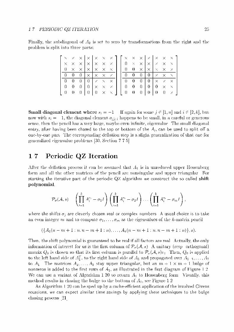
1.7. PERIODIC QZ ITERATION 25Finally, the subdiagonal of A2 is set to zero by transformations from the right and theproblem is split into three parts:2666666664� � � � � � �� � � � � � �0 � � � � � �0 0 0 � � � �0 0 0 0 � � �0 0 0 0 � � �0 0 0 0 0 � �
37777777752666666664� � � � � � �0 � � � � � �0 0 � � � � �0 0 0 0 � � �0 0 0 0 � � �0 0 0 0 0 � �0 0 0 0 0 0 �
3777777775Small diagonal element where si = �1. If again for some j 2 [1; n] and i 2 [2; k], butnow with si = �1, the diagonal element ajj; i happens to be small, in a careful or generoussense, then the pencil has a very large, maybe even in�nite, eigenvalue. The small diagonalentry, after having been chased to the top or bottom of the Ai, can be used to split o� aone-by-one part. The corresponding de ation step is a slight generalization of that one forgeneralized eigenvalue problems [30, Section 7.7.5].1.7 Periodic QZ IterationAfter the de ation process it can be assumed that A1 is in unreduced upper Hessenbergform and all the other matrices of the pencil are nonsingular and upper triangular. Forstarting the iterative part of the periodic QZ algorithm we construct the so called shiftpolynomial,P�(A; s) = kYi=1 Asii � �1I! kYi=1 Asii � �2I! : : : kYi=1 Asii � �mI! ;where the shifts �j are cleverly chosen real or complex numbers. A usual choice is to takean even integer m and to compute �1; : : : ; �m as the eigenvalues of the k-matrix pencil(fA1(n�m + 1 : n; n�m + 1 : n); : : : ; Ak(n�m + 1 : n; n�m+ 1 : n)g; s):Then, the shift polynomial is guaranteed to be real if all factors are real. Actually, the onlyinformation of interest for us is the �rst column of P�(A; s). A unitary (resp. orthogonal)matrix Q0 is chosen so that its �rst column is parallel to P�(A; s)e1. Then, Q0 is appliedto the left hand side of AT1 , to the right hand side of Ak and propagated over Ak�1; : : : ; A2to A1. The matrices A2; : : : ; Ak stay upper triangular, but an m + 1 � m + 1 bulge ofnonzeros is added to the �rst rows of A1, as illustrated in the �rst diagram of Figure 1.2.We can use a variant of Algorithm 1.20 to return A1 to Hessenberg form. Visually, thismethod results in chasing the bulge to the bottom of A1, see Figure 1.2.As Algorithm 1.20 can be sped up by a cache-e�cient application of the involved Givensrotations, we can expect similar time savings by applying these techniques to the bulgechasing process [21].

26 CHAPTER 1. THE PERIODIC QZ ALGORITHM
Figure 1.2: Diagrams of the bulge chasing process.Computation of the initial bulge Especially for long products, computing the shiftsand the shift polynomial desires for great care to avoid unnecessary over-/under ow anddisastrous cancellations. From this point of view, it is more favorable to construct the initialtransformation Q0 directly from the given data. For example, if the shift polynomial canbe rewritten as a product of matrices, then Q0 can be computed by a partial product QRfactorization [22]. For the case m = 2 with �1; �2 as the eigenvalues of the south east2-by-2 pencil such a suitable product embedding is given byP�(A; s) = � A1 In � � kYi=2 � Ai 00 an�1;n�1; iIn �si� � �In 0an�1;n�1; 1In �an;n�1; 1In �� �A1 an;n�1; 1In an;n; 1In0 an�1;n�1; 1In an�1;n; 1In �(1.21)� kYi=2 24 Ai 0 00 an�1;n�1; iIn an�1;n; iIn0 0 an;n; iIn 35si � 24 In0In 35 :By carefully exploiting the underlying structure the recursive computation of Q0 from thisembedding requires approximately 37k ops. For further details the FORTRAN 77 routinePLASHF should be consulted.It is unlikely to �nd an embedding like (1.21) for larger m. Thus, we propose to reducethe m-by-m south east pencil to Schur form, group m=2 pairs of complex conjugate or real

1.8. EXPLOITING THE SPLITTING PROPERTY 27eigenvalues together and apply the partial product QR decomposition to the product ofm=2 corresponding embeddings 1.21). However, it must be noted that the complexity ofsuch an algorithm becomes O(km3). On the other hand, from the experiences with QRalgorithms [72] it can be expected that useful m are less than 10.1.8 Exploiting the Splitting PropertyConvergence is certainly the most important aspect of an iterative algorithm.Consider the k-matrix pencil (A; s) withA1 = 26666664 9:0 4:0 1:0 4:0 3:0 4:06:0 8:0 2:0 4:0 0:0 2:00:0 7:0 4:0 4:0 6:0 6:00:0 0:0 8:0 4:0 6:0 7:00:0 0:0 0:0 8:0 9:0 3:00:0 0:0 0:0 0:0 5:0 0:037777775 ; (1.22)
A2 = � � � = Ak = diag(10�1; 10�2; 10�3; 1; 1; 1);and s2 = � � � = sk = 1. For k = 5 the periodic QZ algorithm requires 29 iterations toconverge, 62 for k = 10, 271 for k = 40 and for k � 50 it does not converge at all. Evenworse, the breakdown cannot be cured by using standard ad hoc shifts.The reason is basically that the leading diagonal entries in the triangular factors divergeexponentially, that is, the relationkYi=1 a(i)j+1;j+1a(i)jj !si = O(�k); 0 � � < 1; (1.23)is satis�ed for j = 1; 2. A Givens rotation acting on such a (j; j + 1) plane is likely toconverge to the 2-by-2 identity matrix when propagated over Ak; Ak�1; : : : ; A2 back to A1.It is important to note that (1.23) is not an exceptional situation. Exponentially splitproducts as de�ned by Oliveira and Stewart [56] have the pleasant property that even forextremely large k the eigenvalues can be computed to high relative accuracy. Moreover,such products hardly ever fail to satisfy (1.23). One of the prominent examples is an in�niteproduct where all factors have random entries chosen from a uniform distribution on theinterval (0; 1). It can be shown that the sequence of periodic Hessenberg forms related to�nite truncations of this product satis�es (1.23) for all j = 1; : : : ; n� 1.For the purpose that exponentially diverging diagonal entries do not represent a con-vergence barrier the following additional de ation strategy is proposed.A QR decomposition is applied to the Hessenberg matrix A0. If sk = 1, the resultingn� 1 Givens rotations (cj; sj) are successively applied to the columns of Ak," a(k)j;j a(k)j+1;j0 a(k)j+1;j+1 # � cj sj�sj cj �= " cja(k)j;j � sja(k)j+1;j sja(k)j;j + cja(k)j+1;j�sja(k)j+1;j+1 cja(k)j+1;j+1 # :

28 CHAPTER 1. THE PERIODIC QZ ALGORITHMWhenever it happens that ��sja(k)j+1;j+1�� is small compared tomax���cja(k)j;j � sja(k)j+1;j��; ��cja(k)j+1;j+1���;or, being more generous, compared to kAkk, then in the following steps (cj; sj) can be safelyset to (1; 0). Otherwise, the (j + 1; j) element of Ak is annihilated by a Givens rotationacting on rows (j; j + 1). (cj; sj) is overwritten with the parameters of this rotation.The process, being similar when sk = �1, is recursively applied to Ak�1; : : : ; A2. At theend, the rotation sequence is applied to the columns of A1 and each pair (cj; sj) = (1; 0)results in a zero element at position (j + 1; j) in A1.Since the above procedure is as expensive as a single shift periodic QZ iteration itshould only occasionally be applied.For the k-matrix pencil (1.22) with k = 40, two applications of the proposed de ationstrategy result in zeros at positions (2; 1), (3; 2) and (7; 6) in A1. Barely 7 periodic QZiterations are required to reduce the remaining 3-by-3 product to quasi upper triangularform.1.9 Shifts in a BulgeDuring the chasing process shifts are carried by the bulge down to the bottom of theHessenberg matrix in order to force a de ation at the (n�m+1; n�m) position. Watkins[71, 72] observed for the QR and QZ algorithms that the shifts can actually be computedfrom the current bulge. Furthermore, it was pointed out that there is an almost one-to-onecorrespondence between the quality of shifts in a bulge and rapid convergence. Needlessto say, there is an easy generalization to periodic eigenvalue algorithms.Let us consider a k-matrix pencil (A; s) in periodic Hessenberg form, where s1 = 1and A1 is unreduced upper Hessenberg. Furthermore we will assume that all zero diagonalentries of the upper triangular matrices Ai with si = 1 are de ated and therefore do notexist. Note that nevertheless in�nite eigenvalues are welcome unless they do not appear inthe upper m � m portion of the matrix pencil. In that case the �rst column of the shiftpolynomial were not well-de�ned.First, let us de�ne the so called zeroth bulge pencil. Given m shifts, we calculatex = �P�(A; s)e1 = � kYi=1 Asii � �1I! : : : kYi=1 Asii � �mI! e1; (1.24)where � is any convenient nonzero scale factor. The vector x has at most m + 1 nonzeroentries.Now, de�ne the zeroth bulge pencil as the (k + 1)-matrix pencil(C; ~s) := (fC1; N; C2; C3; : : : ; Ckg; fs1;�1; s2; s3; : : : ; skg); (1.25)where N is a single (m+ 1)-by-(m+ 1) zero Jordan block andC1 = 26664 x1 a11:1 : : : a1m:1... a21:1 . . . ...... 0 . . . amm:1xm+1 0 0 am+1;m:137775 ; Ci = 26664 a11:i : : : a1m:i 0. . . ... ...amm:i 01 37775

1.9. SHIFTS IN A BULGE 29with i = 2; : : : ; k. Now, we are ready to rewrite [71, Theorem 5.1] for periodic eigenvalueproblems.Corollary 1.21 For a given k-matrix pencil (A; s) in unreduced upper Hessenberg formsuppose that for i = 2; : : : ; k,ajj:i 6= 0 for � j � m; si = �1;j = 1 : : : n; si = 1:Then the eigenvalues of the zeroth bulge pencil (C; ~s) as de�ned in (1.25) are the shifts�1; : : : ; �m and 1.Proof: By assumption, the matrix product B = A�skk A�sk�1k�1 : : : A�s22 is well de�ned.We apply [71, Theorem 5.1] to the generalized eigenvalue problemC1 � � ~B; ~B = � 0 B(1 : m; : m)0 0 � ;and �nd that its �nite eigenvalues are given by �1; : : : ; �m. The (m + 1)-by-(m+ 1)matrix ~B can be factorized as ~B = C�snn Csn�1n�1 : : : C�s22 N; which completes the proof.Applying the orthogonal transformation Q0 with Q0x = e1 to both sides of the productresults in the formation of a bulge in A0. The rest of the periodic QZ iteration consistsof returning the pencil to Hessenberg-triangular form by chasing the bulge from top tobottom. Say the bulge has been chased j� 1 positions down and to the right. The currentpencil (A(j); s) has a bulge in A1 starting in column j. The tip of the bulge is at aj+m+1;j:1; 1.The j-th bulge pencil is de�ned as(C(j); ~s) = (fC(j)1 ; N; C(j)2 ; C(j)3 ; : : : ; C(j)k g; fs1;�1; s2; s3; : : : ; skg); (1.26)where N again denotes a single (m+ 1)-by-(m+ 1) zero Jordan block andC(j)1 = 26664 aj+1;j:1 : : : aj+1;j+m:1... ...aj+m;j:1 : : : aj+m;j+m:1aj+m+1;j:1 : : : aj+m+1;j+m:137775 ; C(j)i = 26664 aj+1;j+1:i : : : aj+1;j+m:i 0. . . ... ...aj+m;j+m:i 01 37775for i = 2; : : : ; k.The following corollary can be considered as a periodic variant of [71, Theorem 5.2].Corollary 1.22 Under the assumptions of Corollary 1.21 the �nite eigenvalues of the j-thbulge pencil as de�ned in (1.26) are the shifts �1; : : : ; �m.Proof: The proof goes along the lines of the proof of Corollary 1.21, now applying [71,Theorem 5.2] on the corresponding collapsed pencil.Remark 1.23 In the previous section we saw that pencils with exponentially divergingfactors may su�er convergence breakdowns. This is essentially caused by an impropertransmission of shifts. After having chased the bulge to the bottom one could checkwhether it still contains a passable approximation to the shifts. If this is not the casefor small m, then it is certainly a good time to apply a controlled zero shift iteration.

30 CHAPTER 1. THE PERIODIC QZ ALGORITHMShould we still de ate in�nite eigenvalues ? Watkins [71] states: It would be muchmore e�cient to use the upward-chasing analogue of [30, 7.7.5] which de ates in�niteeigenvalue at the top. Better yet, one can let the QZ algorithm deal with the zeros..Let us discuss the denial of de ating in�nite eigenvalues, unless they do not appear inthe top of the pencil.For a discussion it is su�cient to consider the single shift algorithm for the generalizedeigenvalue problem A � �B. Assume that there is one zero diagonal element at the (j; j)position in B. We want to distinguish between computing the complete Schur form andthe exclusive computation of eigenvalues. In both cases de ating the in�nite eigenvaluescuts the trip of the bulge in the subsequent QZ step by exactly one element. In the lattercase additional savings can be achieved, since then the orthogonal updates are applied toa smaller subpencil. On the other hand, de ating in�nite eigenvalues is not a free dinner.From the viewpoint of e�ciency one clearly wants to chase the in�nite eigenvalue to thetop if j � n2 and to the bottom if j > n2 .Table 1.5 lists the necessary operations for de ating one in�nite eigenvalue and thesubsequent j single shift QZ steps. The integer function fj(n) denotes the number ofoperations which are necessary for applying j QZ steps without any de ation. Only O(n2+nj) terms are displayed. By denying de ation we have to apply approximately fj(n)Generalized Eigenvalues Generalized Schur decompositionj � n2 fj(n)� 12nj fj(n)j > n2 fj(n) + 12n2 � 36nj fj(n) + 12n2 � 24njTable 1.5: Flop counts for the de ation of in�nite eigenvalues.operations until we get a de ation of the in�nite eigenvalue at the top. As observed in [71]the quality of the bulge pencil tends to be invariant under de ation. However, in all casesthe expenses for de ation are less or equal than the costs of a denial of de ation. Thisstatement is even stronger when the orthogonal transformations have to be accumulated.To summarize, we answer the question in the title: Yes, we should still de ate in�niteeigenvalues.1.10 An ApplicationWe want to �nish this chapter with a less known application of the periodic QZ algorithm.It will also be shown that the ideas of Section 1.5.2 can be applied to Hessenberg-triangularreduction algorithms for di�erently structured matrices.Benner, Byers, Mehrmann and Xu [6] developed methods for several structured gener-alized eigenvalue problems. The main part of the computation consists of a reduction tosome sort of Hessenberg form and one application of the periodic QZ algorithm. From thecorresponding condensed form it is an easy task to extract the eigenvalues of the underlying(generalized) Hamiltonian problem. Note that all the Hessenberg like reduction algorithmsin [6] mainly consists of Givens rotations. As mentioned earlier, modern computer archi-tectures do not love these BLAS 1 techniques. Fortunately, we can block the Hessenberg

1.10. AN APPLICATION 31reduction algorithms by a method which is quite similar to the methods described in Sec-tions 1.5.2 and 1.5.3. Let us demonstrate the technique by a reformulation of [6, Algorithm3].NotationDe�nition 1.24 Let J := � 0 In�In 0 �, then1. a matrix H 2 C 2n;2n is Hamiltonian if (HJ)H = HJ,2. a matrix S 2 C 2n;2n is skew-Hamiltonian if (SJ)H = �SJ,3. a matrix S 2 C 2n;2n is symplectic if SJSH = J, and4. a matrix Ud 2 C 2n;2n is unitary symplectic if UdJUHd = J and UdUHd = I2n.We are not going to explore the beautiful algebraic structures, like Lie algebras or Jordangroups, induced by these matrices. Only these relations are listed below which are usefulfor our further considerations.1. H = � H11 H12H21 H22 � is Hamiltonian if and only if H21 and H12 are symmetric andH11 = �HH11.2. H = � S11 S12S21 S22 � is skew-Hamiltonian if and only ifH21 and H12 are skew-symmetricand S11 = SH11.3. The unitary symplectic matrices form a group with respect to multiplication (in facteven a Lie group).4. For a skew-Hamiltonian S and unitary symplectic U the matrix JUHJHSU is alsoskew-Hamiltonian.Some examples for unitary symplectic matrices The de�nition of a unitary sym-plectic matrix excludes some useful unitary transformations like all Householder re ectionslarger than n-by-n. It is well known that Q 2 C 2n;2n is unitary and symplectic if and onlyif Q = � Q1 Q2�Q2 Q1 � ;where QH1 +QH2 Q2 = In and QH2 Q1 is Hermitian. Nevertheless there are still some usefultransformations in this class. The 2n� 2n Givens rotation matrixGs(i; �) = 266664 Ii�1 cos � sin �In�1� sin � cos � In�i377775

32 CHAPTER 1. THE PERIODIC QZ ALGORITHMas well as Q�Q, for an n-by-n orthogonal matrix Q, are unitary symplectic.As announced, we now present a blocked version of [6, Algorithm 3] which does a Schurlike reduction of real skew-Hamiltonian / skew-Hamiltonian matrix pencils.Algorithm 1.25 Given a real skew-Hamiltonian / skew-Hamiltonian pencil(fS;Ng; f�1; 1g)with S = JZTJTZ, the algorithm computes an orthogonal matrix Q and an orthog-onal symplectic matrix U such thatUTZQ = � Z1 ?Z2 � and JQTJTNQ = � N1 ?N1 � ;with upper triangular Z1; ZT2 and upper quasi triangular N1.Step 1 Apply a blocked RQ factorization with changed elimination order to Z to de-termine an orthogonal Q such thatZ ZQ = 264 0 375 :Update N JQTJTNQ using WY representations of the Householder re ec-tions generated by the RQ factorization.Step 2 For the readers convenience this step is only illustrated for n = 9 with blocksize r = 3. The (i; j) block entry is denoted by Zij and Nij, respectively.We start with an RQ factorization of � N41 N42 � which introduces nonzerosin Z21 and the lower triangular parts of Z11 and Z22.����
��������������������
��������
����
��������������������
������������������������
��������������������
��������������������
���������
���
����������������
��������
����
����
����������������
��������������������������������
����������������
����������������
����������������
��������������������������������
����������������
����������������
����������������
��������������������������������
����������������
������������
������������������������
����
����������������
������������
����������������
����������������
������������
����������������
������������������������ �
�����������
������������
��������
����������������
������������������������������������
������������
��������
����������������
������������
��������
������������
������������
����
����������������������������������
��������������
����������������
������������������������
����������������
������������
����������������
������������
����
����������������
������������
������������
��������������������
��
����
����������
These entries are immediately annihilated by a QR factorization of � Z11 Z12Z21 Z22 �.To keep things symplectic we have to apply QT also to � Z44 Z45Z54 Z55 � whichunfortunately creates some nonzeros there.

1.10. AN APPLICATION 33��������������������������������
������������������������������������������������
��������������������������������
������������������������������������������������
������������
������������
��������
���������������� ������������������������
������������
������������
��������
���������������� �
�����������
������������
��������
���������������� ������������������������
������������
������������
��������
����������������
����
����������������
����
����������������
��������
��������������������������������
����
����������������
������������
��������������������
����������������
������������
����
����������������
������������
��������������������
����������������
������������
Now we use an LQ factorization of � Z44 Z45Z54 Z55 � to annihilate its upper trian-gular part.��������������������������������������������������������������������������������
������������������������
����������������
����������������������������������������
����
����������������
������������
����������������
����������
��������
��
����������
��������������������
����������������
����
��������������������
����������
��������
��
����������
����������
��������
��
����������
����������
��������
��
����������
��������������������
����������������
����
��������������������
����
����������������
������������
����
����������������
������������
��������������������
����������������
������������
����
����������������
������������
��������������������
����������������
������������
����
����������������
������������
��������������������
����������������
������������
������
��������
������
������
����
������
��������
������
������
����
������������
����������������
������������
������������
��������
������
��������
������
������
����
������
��������
������
������
����
������������
����������������
������������
������������
��������
����������������
������������������������
����������������
������������������������
������������
������������������������������������
���� ������������ ��������������������
������������������������������������
������������
������������������������������������
���� ������������ ��������������������
������������������������������������
Repeating this process, now starting with an RQ factorization of � N42 N43 �,yields the following diagram.
As long as the block size is su�ciently large, N43 can be quartered and someparts of it get annihilated by the same method as above. However, at theend there are some tiny blocks left which must be annihilated by applying [6,Algorithm 3].The next step consists of a QR factorization of � N21 N31 � creating somenonzero parts in Z.

34 CHAPTER 1. THE PERIODIC QZ ALGORITHM����
����������������
������������
��������������������
����������������
������������
����
����������������
������������
��������������������
����������������
������������
����
����������������
������������
��������������������
����������������
������������
����
����������������
������������
��������������������
����������������
������������
����
����������������
������������
��������������������
����������������
������������
������������
������������
������������������
��������������������������������������������
������������������������������������������������������������������������������������������
����
��������������������������������������������������������������������������������
��������������������������������
��������������������������������������������������������������������������������������������������������������������������������
������������������������������������������������������������
����������������
������������������
����������������������������������������������
����������������
��������������������
��������
����
����
����
���� ��������
�� ��������
��������������������������
��������������
����
��������
�� ����������
����
��������������
Next, we do a QL factorization of � Z55 Z56Z65 Z66 �, which, to keep things symplec-tic, also acts on the upper part of Z.������������
������������
��������
����������������
������������������������������������
������������
��������
����������������
������������
������������
��������
����������������
������������������������������������
������������
��������
����������������
����
����������������
������������
��������������������
����������������
������������
����
����������������
������������
��������������������
����������������
������������
����������������
������������������������
����������������
������������������������
��������������������������������
������������������������������������������������
��������������������������������
������������������������������������������������A suitable RQ factorization annihilates the unwanted nonzero entries in Z whilepreserving the zero structure of N .
��������������������������������
����������������������������������������������������������������
������������������������������������������������
��������������������
����������������
��������������������������������
����������������
������������
������������������������������������
������������
��������
����������������
������������
������������
��������
����������������
������������������������������������
������������
��������
����������������
������������
������������
����
����������������������������
�������������
�������
����������������
������������������
����������������
����
����������������
������������
��������������������
����������������
������������
����
����������������
������������
��������������������
����������������
������������
����
����������������
������������
��������������������
����������������
������������
������������
������������
��������
������������
����
������
Applying the whole step on the remaining submatrices results in somethingwhich might be regarded as an upper r-Hessenberg form for Skew-Hamiltonian/ Skew-Hamiltonian pencils.
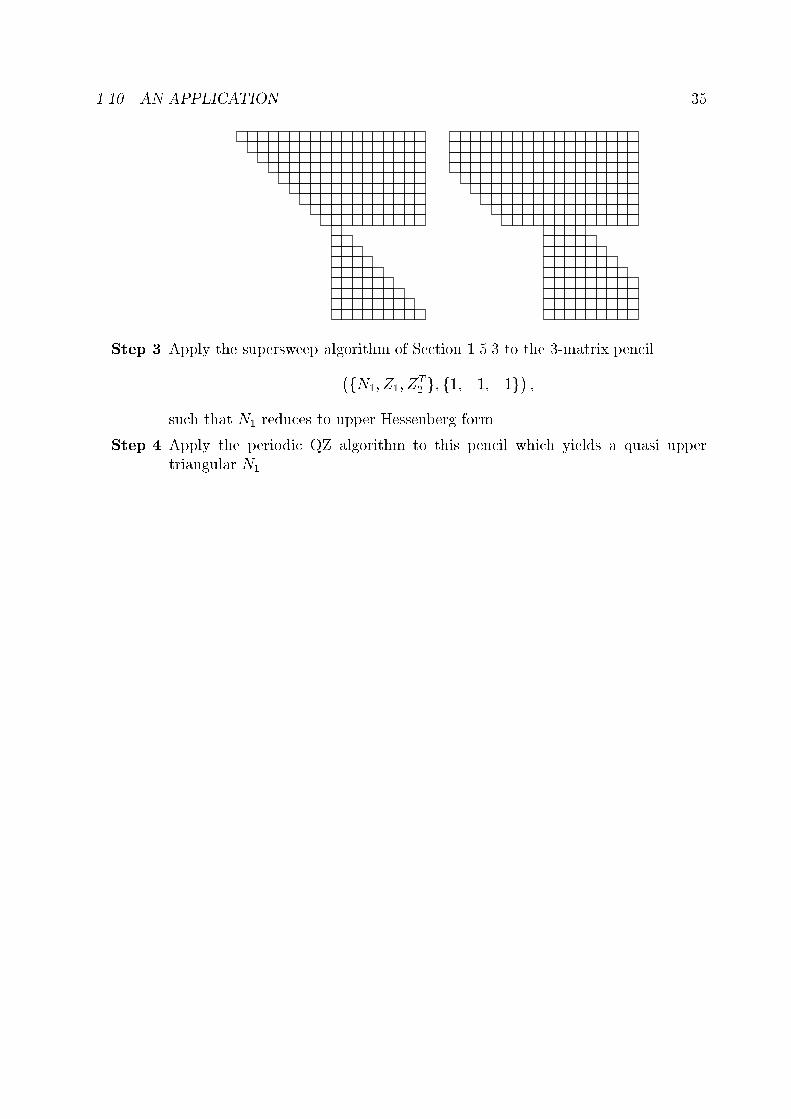
1.10. AN APPLICATION 35
Step 3 Apply the supersweep algorithm of Section 1.5.3 to the 3-matrix pencil�fN1; Z1; ZT2 g; f1;�1;�1g� ;such that N1 reduces to upper Hessenberg form.Step 4 Apply the periodic QZ algorithm to this pencil which yields a quasi uppertriangular N1.

36 CHAPTER 1. THE PERIODIC QZ ALGORITHM
Chapter 2Fast Algorithms for Matrices withBlock Displacement StructureFast algorithms for matrix inversion, (least squares) solution of linear equations and tri-angular and orthogonal matrix factorizations are well known for Toeplitz and Toeplitz-likematrices. The concept of displacement structure was introduced by Kailath and severalcoauthors to show that fast algorithms can also be obtained for a much broader class ofmatrices [41]. Several compositions of Toeplitz matrices as well as matrices which are lowrank perturbations of structured matrices are nowadays well understood in the frameworkof this concept.Factorizations and linear system solvers for such matrices have a wide range of appli-cations. This includes state-space identi�cation, interpolation problems, linear-phase andadaptive �ltering. An extensive overview may be found in [40]. For example, identi�cationsproblems desire for QR factorizations of block Toeplitz matrices [47, 54, 59]. This sectiontreats existing and new approaches for factorizations and (least squares) solutions of sys-tems involving such matrices. Furthermore, numerical results substantiate the stabilityclaims of Stewart and Van Dooren [63].All described algorithms have been implemented in Fortran 77. The codes conform tothe implementation and documentation standards of the software library SLICOT [7, 75].Indeed, most of the routines are already included in this library [43].2.1 IntroductionConsider the linear time-invariant state-space modelxk+1 = Axk +Buk + wk;yk = Cxk +Duk + vk;where uk and yk are the m-dimensional input vector and the l-dimensional output vector,respectively and xk is the n-dimensional state vector at time k and fwkg, fvkg are stateand output disturbances or noise sequences. A, B, C and D are unknown real matrices ofappropriate dimensions.At the "Database for the Identi�cation of Systems", http://www.esat.kuleuven.ac.be/sista/daisy/, one can �nd input/output data sets for such models of glass ovens,37
38 CHAPTER 2. MATRICES WITH BLOCK DISPLACEMENT STRUCTUREevaporators or even CD player arms [53].In non-sequential data processing, one chooses N � 2(m + l)s and constructs theN -by-2(m + l)s matrixH =
2666666666664uT1 uT2 : : : uT2s yT1 yT2 : : : yT2suT2 : : : ... yT2 : : : ...... : : : ... ... : : : ...uT2s uTN yT2s yTN... : : : uTN+1 ... : : : yTN+1... : : : : : : ... ... : : : : : : ...uTN uTN+1 : : : uTN+2s�1 yTN yTN+1 : : : yTN+2s�1
3777777777775 (2.1)consisting of two concatenated block Hankel matrices. Then the R factor of a QR factor-ization H = QR is used for data compression [54, 59, 66]. H becomes a block Toeplitzmatrix by suitable column permutations. One of the results in this section shows that Rcan be computed in no more than O(N rank H) ops.Before comparing accuracy and e�ciency of such fast methods with standard algorithmslike the Householder QR factorization let us focus on a theoretical treatment of blockToeplitz-like matrices and their relatives.2.2 Notion of Block DisplacementLet F f 2 Rm;m and F b 2 Rn;n be strictly lower triangular matrices. For a matrix A 2 Rm;nthe transformation r(F f ;F b)A := A� F fA(F b)T (2.2)is called the displacement of A with respect to the displacement operators fF f ; F bg.A generator of A is a matrix pair fX; Y g withr(F f ;F b)A = XY T ; X 2 Rm;� ; Y 2 Rn;� : (2.3)The integer � measures the length of the generator. A generator of minimal possiblelength is called a minimal generator. The displacement rank of A is de�ned by thelength of the minimal generator, which is equivalent to the rank of r(F f ;F b)A. This conceptof displacement was established by Kailath and Sayed [40]. It should be noted that thereexists another early de�nition of matrices of structure. The book of Heinig and Rost [34]treats matrices for which rA = FA + AGT has low rank for suitable matrices F andG. The two de�nitions are quite similar and parallel tracks for describing Toeplitz-likematrices. In linear system theory, expressions of the form A� FAF T and FA + AF T areassociated with Lyapunov equations for discrete-time and continuous-time systems, whichcan be transformed into each other by well known formulas [38].The displacement of a symmetric matrix A is again symmetric and by Sylvesterslaw of inertia [30, Section 8.1.5] it can be written as r(F;F )A = X�XT where � =diag(�1; : : : ;�1). Under this circumstances we call X a symmetric generator withrespect to the displacement operator F and the signature matrix �.

2.2. NOTION OF BLOCK DISPLACEMENT 39Generators are not unique. If fX; Y g is a generator for A with respect to fF f ; F bg, thenfor any nonsingular matrix S 2 R�;� , the matrix pair fXS; Y S�Tg is also a generator [40,pg. 300]. For symmetric generators the transformation matrix is supposed to be �-unitary,that is, ST�S = S�ST = �.Example 2.1 Consider a symmetric positive de�nite block Toeplitz matrixT = 26664 T0 T T1 : : : T Tn�1T1 . . . . . . ...... . . . . . . T T1Tn�1 : : : T1 T037775 ; T0 = T T0 ; Ti 2 Rk;k ; i = 0; : : : ; n:T0 as the leading k-by-k submatrix of T is always positive de�nite. With respect tothe following displacement operator and signature matrixF := Zk = 26664 0Ik . . .. . . . . .Ik 0
37775 ; �kk = � Ik 00 �Ik � ;we obtain the generatorXT = � L�10 00 L�10 � � T0 T T1 T T2 : : : T Tn�10 T T1 T T2 : : : T Tn�1 � (2.4)by inspection. Here, L0 denotes the lower triangular Cholesky factor of T0, i.e., T0 =L0LT0 . Hence, we have shown that the displacement rank is at most 2k. Furthermore,X is minimal if and only if the matrix [T1 T2 : : : Tn�1] has full rank.It is important to note that a matrix is completely determined by its generators. LetA and X; Y satisfy equation (2.3), then it can be shown [39] thatA = �Xi=1 Kn(xi; F f)KTn (yi; F b); (2.5)where xi and yi are the i-th column of X and Y , respectively, and Kn(z; B) denotes theKrylov matrix Kn(x;B) = � z Bz B2z : : : Bn�1z � :As we will see later, inverses of Toeplitz matrices have low displacement rank, thus equation(2.5) can be seen as a generalization of the Gohberg-Semencul formula [28].When dealing with matrices with block structure it is more natural to use block repre-sentations of generators. For this purpose it is assumed that F f and F b are strictly lowertriangular with k�1 zero subdiagonals. This condition assures that all the well known def-initions and theorems for displacement structured matrices may be reformulated in k-by-kblock form. The notion of proper generators plays a key role in these observations.

40 CHAPTER 2. MATRICES WITH BLOCK DISPLACEMENT STRUCTUREDe�nition 2.2 A generator pair fX; Y g is called proper if it has the formX = " k ��kk X11 0m�k X21 X22 #; Y = " k ��kk Y11 0n�k Y21 Y22 #: (2.6)2.3 The generalized Schur algorithmA fundamental method for triangular matrix factorization is the so-called Schur reduc-tion process [39, 40, 58]. This algorithm computes the Schur complements of the leadingsubmatrices iteratively; displacement structure allows the computation to be sped up. Allfast Schur algorithms are based on a variant of the following theorem.Theorem 2.3 Assume that fX; Y g is a proper generator pair of A, partitioned as in (2.6).Then the matrix ~A = A�X1�Y T1� (2.7)has k zero leading columns and rows. A generator pair f ~X; ~Y g for ~A is given by~X = � F fX1� X2� � ; ~Y = � F fY1� Y2� � ; (2.8)where F f and F b are as in (2.2).Proof: Setting E1 = [Ik 0 : : : 0]T we prove the �rst part by observing that~AE1 = (A�X1�Y T1� )E1 = F fA((F b)TE1) = 0ET1 ~A = ET1 (A�X1�Y T1� ) = ((F f)TE1)TA(F b)T = 0;stressing the fact that fX; Y g is proper and F f ; F b are lower triangular with a zeroleading k-by-k submatrix. Furthermore, we have~A� F f ~AF b = (A�X1�Y T1� )� F f(A�X1�Y T1� )(F b)T= (A� F fA(F b)T )�X1�Y T1� + F fX1�Y T1� (F b)T= XY T �X1�Y T1� + F fX1�Y T1� (F b)T= ~X ~Y T ;which completes the proof.The above theorem is a block formulation of the well-known special case k = 1 [39].It enables us to apply k Schur steps at once and to use blocking techniques as alreadydescribed in [25].The following lemma characterizes the role of ~A in Theorem 2.3.

2.3. THE GENERALIZED SCHUR ALGORITHM 41Lemma 2.4 Under the assumptions of Theorem 2.3 partitionA = � k n�kk A11 A12m�k A21 A22 �; ~A = � k n�kk 0 0m�k 0 ~A22 �:If A11 is nonsingular then ~A22 is the Schur complement of the leading k-by-k subma-trix of A, that is, ~A22 = A22 � A21A�111 A21: (2.9)Proof: By equation (2.7) we haveA11 = X11Y T11; A12 = X11Y T21; A21 = X21Y T11; A22 � ~A22 = X21Y T21;and henceA22 � A21A�111 A12 = ~A22 +X21Y T21 �X21Y T11(X11Y T11)�1X11Y T21 = ~A22:Note that it is not always possible to construct proper generators, for example thegenerator pair fX; Y g = �� 1 0 � ; � 0 1 �clearly has no proper generator representation for k = 1. The product singular valuedecomposition (SVD) [24, 52, 55] turns out to be a useful tool to classify such pathologicalcases.Lemma 2.5 Given a generator pair fX; Y g with X and Y as in (2.2), there exists anonsingular matrix S 2 Rn;n and orthogonal matrices U; V 2 Rk;k such thatUX1�S = " rX n�rXrX I 0k�rX 0 0 # (2.10)and V Y1�S�T = 264 rY 1 rX�rY 1 rY 2 n�(rX+rY 2)rY 1 S1 0 0 0rY 2 0 0 S2 0k�rY 1�rY 2 0 0 0 0 375 (2.11)where S1 and S2 are diagonal matrices with positive entries.Proof: The proof follows by applying the product SVD [52, Theorem 1.1] to X1�Y T1� .

42 CHAPTER 2. MATRICES WITH BLOCK DISPLACEMENT STRUCTUREObserve that the block sizes in the decomposition (2.10, 2.11) can be obtained by thefollowing relationsrX = rank X1�; rY 1 + rY 2 = rank Y1�; rY 1 = rank X1�Y T1� :Inspecting the blocks in (2.10) and (2.11) we see that it is possible to construct a propergenerator representation if and only if rX + rY 2 � k. This leads toTheorem 2.6 Given a generator pair fX; Y g with X and Y as in (2.2), there exists anonsingular matrix S such that fXS; Y S�Tg is proper if and only ifrank X1� + rank Y1� � rank X1�Y T1� � k: (2.12)Condition (2.12) is not very strong as shown by the following corollary.Corollary 2.7 Let A 2 Rn;n be a matrix with leading nonsingular k-by-k submatrix andsatisfy a displacement equation (2.2). Then the corresponding generator pair fX; Y ghas a proper generator representation.Proof: The leading k-by-k submatrix of A is given by A11 = X1�Y T1� . Hencerank X1� + rank Y1� � rank X1�Y T1� = rank X1� + rank Y1� � k � k:Applying Theorem 2.6 yields the result.Assembling Theorem 2.3, Lemma 2.4 and Theorem 2.6 gives the following algorithm.Algorithm 2.8 Given A 2 Rm;n and a generator pair fX; Y g as in (2.2), the followingalgorithm computes the incomplete block LU factorizationA = LU � ~A= 2666664 L11... . . .Li1 : : : Lii... ...Lm1 : : : Lmi37777752666664 U11... . . .Ui1 : : : Uii... ...Un1 : : : Uni
3777775T � � 0 00 AS �where i � min(bm=kc; bn=kc) is the number of applied Schur steps and AS is theSchur complement of the leading ik-by-ik block in A. AS is presented in terms of itsgenerators.for j = 1: i doif rank X1� + rank Y1� � rank X1�Y T1� � k thenTransform fX; Y g to proper form as described in the proof of Lemma 2.5.Update L = � L 0X�1 � and U = � U 0Y�1 � :Set X = � F fX1� X2� � and Y = � F bY1� Y2� � with F f and F b as in (2.2):Remove the �rst k rows from X and Y .elseBreakdown encountered.endend

2.4. EXPLOITING SYMMETRIES 43Remark 2.91. A square matrix is called strongly nonsingular if all its leading principal sub-matrices are nonsingular. Collorary 2.7 yields in this case that Algorithm 2.8su�ers no breakdown and gives the complete LU factorization after n=k stepsprovided that n is an integer multiple of k.2. In order to call this algorithm fast, the expenses for the matrix-by-vector multi-plications F fX1� and F bY1� should be negligible. Then the complexity of Algo-rithm 2.8 is O(ik3(m+n)), assuming that the minimal generator length satis�es� = O(k).3. An important special case is the LU factorization of a point Toeplitz matrix. Inthe sense of e�ciency the O(n2) Algorithm 2.8 should be preferred to standardO(n3) methods.Stability tells quite a di�erent story. Theoretically, L and U are the sametriangular factors as obtained from Gaussian elimination without pivoting (GE)applied to A. It is well-known that the norms of the triangular factors canbecome arbitrarily large when using GE. However, for a small backward errorit is crucial that the norms of L and U are of magnitude kAk [37, Section 9.2].The norm growth is likely to become large when the condition numbers of theleading principal submatrices are much larger than the condition number of thematrix itself. For such Toeplitz matrices a factorization method which employspivoting is more suitable [14].2.4 Exploiting SymmetriesThe derivation of the condensed form (2.10, 2.11) does not preserve symmetries in thegenerator pair. However, this aspect is crucial in applications.As mentioned before, block structured symmetric matrices A 2 Rn;n usually satisfydisplacement equations of the formr(F;F )A = A� FAF T = X�pqXT ; (2.13)where F has a leading principal k-by-k zero submatrix. For convenience let us assume thatp � k which can be satis�ed whenever p+ q � k. If we partition X asX = � X�p X�q � = � p qk X1p X1qn�k X2p X2q �;then Xp� and X�q are the positive and negative generators of A, respectively. X is properif X1p has only nonzero entries in the �rst k columns and X1q vanishes completely. Thiscertainly results in a stronger condition on X than Theorem 2.6 proposes. Indeed, the �rstblock of A is given by A11 = X1pXT1p �X1qXT1q; (2.14)
44 CHAPTER 2. MATRICES WITH BLOCK DISPLACEMENT STRUCTUREand therefore the existence of a proper representation implies the positive semide�nite-ness of A11. Conversely, when the complete matrix A is positive semide�nite, we get thefollowing theorem.Theorem 2.10 Let A 2 Rn;n be a symmetric matrix satisfying the relation (2.13). If A ispositive semide�nite then there exists a proper generator of A.Proof: Using a generalized SVD [30, Section 8.7.3] of X�11q X1p there exist orthogonalmatrices U 2 Rp;p ; V 2 Rq;q and a nonsingular matrix S such that (2.14) can berewritten as SA11ST = SX1pU(SX1pU)T � SX1qV (SX1qV )T= DpDTp �DqDTq ;where DpRk;p and Dq 2 Rk;q are rectangular diagonal matrices with nonnegativeentries. Sylvesters law of inertia implies that A11 is positive semide�nite if and onlyif jdpij � jdqij; 8i 2 [1; : : : ; k]: (2.15)Here, dpi and dqi denote the i-th diagonal entries of Dp and Dq, respectively. Forq < k missing diagonal entries in Dq are assumed to be zero.Now, set ~X�p := X�pU = S�1Dp and ~X�q := X�qV = S�1Dq. Three situations mayoccur in (2.15):1. jdpij > jdqij: By hyperbolic rotations (see Section 2.5) a �pq-unitary matrix canbe constructed, which, applied to the right hand side of � dpi dqi �T , removesdqi. Applied to the corresponding columns in ~X�p and ~X�q this transformationannihilates the i-th column of ~X1q.2. jdpij = jdqij = 0: This is just �ne, the i-th column of ~X1q is already zero.3. jdpij = jdqij 6= 0: Consider the matrix~A = � ~A11 ~AT21~A21 ~A22 � := � S 00 In�k �A � ST 00 In�k � ;which is by assumption positive semide�nite. The matrix ~A11 = DpDTp �DqDTqis diagonal with a zero at position (i; i). Now, ~A21ei = 0, otherwise one canalways construct a vector x 2 Rn such that xT ~Ax < 0; which violates thesemide�niteness of ~A.From relation (2.13) and the structure of F we have0 = ~AT21ei = � ~X2p � ~X2q � � ~XT1p~XT1q �ST ei= � ~X2p � ~X2q � � DpDq � ei;which yields dqi ~X2pei = dpi ~X2qei and hence ~X�pei = � ~X�qei. We have thus shownthat the i-th columns of ~X�p and ~X�q can be removed from the generator withoutalterning the displacement equation (2.13).

2.4. EXPLOITING SYMMETRIES 45Altogether, two matrices ~X�p and ~X�q have been constructed so that ~X is a propergenerator of A.Corollary 2.11 Let X be a symmetric generator of a matrix A with leading positive def-inite k-by-k block A11. Then there exists a �pq-unitary matrix S such that XS isproper.Proof: The proof is as the proof of Theorem 2.10 only that we now have strict in-equalities in (2.15) which implies that the situations 2 and 3 do not occur. Only�pq-unitary transformations are applied to reduce X to proper form.The stronger condition in Corollary 2.11 yields the existence of a proper generator withthe same minimal length.Singularity of A11 leads to a di�erent formulation of Lemma 2.4.Lemma 2.12 Let A be a symmetric positive semide�nite matrix and let X be a propergenerator of A in the sense of relation 2.13. Then� A11 A12AT12 A22 ��X�XT = � 0 00 A22 � AT12Ay11A21 � :Proof: The positive semide�niteness of A implies that kernel A11 � kernel AT12. There-fore� I 0�AT12Ay11 I � � A11 A12AT12 A22 � � I �Ay11A120 I � = � A11 00 A22 � AT12Ay11A12 � :Now, the result follows from analogous considerations as in the proof of Lemma 2.4.Assembling Theorem 2.3, Theorem 2.10 and Lemma 2.12 gives rise to an algorithm forsymmetric positive semide�nite matrices with structure. In contrast to Algorithm 2.8 ittheoretically never fails.Algorithm 2.13 Given a symmetric positive semide�nite matrix A with generator X, thefollowing algorithm computes the incomplete block Cholesky factorizationA = LLT � ~A= 2666664 L11... . . .Li1 : : : Lii... ...Lm1 : : : Lmi3777775264 LT11 : : : LTi1 : : : LTm1. . . ... ...LTii : : : LTmi 375� � 0 00 AS �where i � bn=kc is the number of Schur steps. AS is presented in terms of itsgenerators.

46 CHAPTER 2. MATRICES WITH BLOCK DISPLACEMENT STRUCTUREfor j = 1 : i doTransform X to proper form by using the construction in the proof ofTheorem 2.10.Update L = � L 0X( : ; 1: k) � :Set X = � FX( : ; 1: k) X( : ; k + 1: p+ q) � where F is as in (2.13):Remove the �rst k rows from X.end2.5 Constructing Proper GeneratorsAvailable Fortran RoutinesMB02CX.f Generator reductionMB02CY.f Application of the generator reduction to further partsAlthough the proofs of Theorem 2.6 and Theorem 2.10 are constructive, they both use somekind of singular value decomposition far from being e�cient. We give a brief summary ofmore elementary transformations which will be used in the following algorithms.Orthogonal transformations Givens rotations, Householder and Block Householderre ectors [30, Section 5.1] belong to this category. These are perfectly stable transfor-mations [37, Chapter 18]. However, there is usually a trade o� between exibility ande�ciency.Hyperbolic rotation We construct a matrix � 2 R2;2 with�T�11� = ��11�T = �11;such that for a given vector [x y] 2 R2 with jyj < jxj,� � xy � =px2 � y2e1:The transformation is given by� = 1p1� �2 � 1 ���� 1 � ; where � = yx: (2.16)Note that the norm of � gets close to in�nity as jyj gets close to jxj. An application of thehyperbolic rotation to the right hand side of the matrix G 2 Rn;2 satis�esG��11(G�)T �G�11GT = 0: (2.17)In a naive implementation as suggested by (2.16) we obtain a computed matrix G = fl(G�)such that [39, Section 2.6.1],kG�11GT �G�11GTk2 � On(")kGk22k�k22: (2.18)

2.5. CONSTRUCTING PROPER GENERATORS 47Since k�k can be arbitrarily large, the computed quantities are unlikely to satisfy (2.17) tosu�cient accuracy.A better implementation is provided by the mixed downdating procedure [39, Section2.6.2] which computes ~G = G� from~G( : ; 1) = 1p1� �2 (G( : ; 1)� �G( : ; 2)); (2.19)~G( : ; 2) = � ~G( : ; 1) +p1� �2G( : ; 2): (2.20)This way the transformation needs 6n ops. Using equations (2.19) and (2.20) to computeG = fl(G�) we can improve inequality (2.18) tokG�11GT �G�11GTk2 � On(")�kGk22 + kGk22� : (2.21)Hyperbolic Householder transformations [11, 20] For a given vector x 2 Rn weconstruct a vector v 2 Rn such thatUxx = ��pq � 2vvTvT�pqv� x = (xT�pqx)e1:The quantity xT�pqx is often called the hyperbolic norm of x [25]. In contrast to hyperbolicrotations, BLAS level 2 routines can be used for the application of Ux. However, thenumerical reliability is questionable. For example, let us consider the matrixG = � 1:01 1 0:0120 3 7 � :Annihilating G(1; 3) with a Givens and G(1; 2) with a Hyperbolic rotation yields a com-puted G which satis�es kG�12GT �G�12 ~GTk2 = 2:5 � 10�13:On the other hand, applying a hyperbolic Householder re ector to annihilate G(1; 2: 3)gives us kG�12GT �G�12 ~GTk2 = 1:2 � 10�11:Additionally, in our applications we often have the situationxT = [ � p�1 timesz }| {0 : : : 0 q timesz }| {� : : : � ];so that it is more e�cient to replace the hyperbolic re ector by one orthogonal re ectorand one hyperbolic rotation.Block hyperbolic Householder transformations [25, 31] The idea of blocking or-thogonal re ectors can be generalized to hyperbolic re ectors. However, even more thanin the previous paragraph reliability claims are unsubstantiated. In fact, neither Gallivanet.al. [25] nor Hallinger [31] give any accuracy results. Thus, we rather propose a combina-tion of Block Householder representations and Hyperbolic rotations which will introducealmost the same fraction of level-3 operations.

48 CHAPTER 2. MATRICES WITH BLOCK DISPLACEMENT STRUCTUREBlock Gaussian elimination Gaussian eliminations are the only unsymmetric oper-ations which will be needed in our applications. Given a matrix G = [ G1 G2 ] withnonsingular G1 the second block is annihilated by the nonsingular transformation� G1 G2 � � I �G�11 G20 I � = � G1 0 � :Now, we have the necessary utilities to present e�cient algorithms for the reduction ofgenerators to proper form. The �rst two presented algorithms assume positive de�nitenessand su�er a breakdown if this condition is not satis�ed.Algorithm 2.14 Unblocked reduction for �pq-symmetric generatorsGiven a generator G 2 Rn;p+q with p � k this algorithm computes a proper repre-sentation of G.1. Compute an LQ factorization such thatG(1 : k; 1: p) = � L 0 �Qwhere L is a k-by-k lower triangular matrix and Q is orthogonal.2. Update G( : ; 1: p) = G( : ; 1: p)QT .3. for i = 1: k doAnnihilate G(i; p+ 2: p+ q) by a Householder re ector V from the right.Update G(i : n; p+ 1: p+ q) = G(i : n; p+ 1: p + q)V:if jG(i; i)j > jG(i; p+ 1)j thenDetermine a hyperbolic rotation � such that� G(i; i) G(i; p+ 1) � � = � � 0 � :Update � G(i : n; i) G(i : n; p+ 1) � = � G(i : n; i) G(i : n; p+ 1) � �:elseBreakdown encountered.endendA straightforward blocked formulation with block size nb is given byAlgorithm 2.15 Blocked reduction for �pq-symmetric generatorsGiven a generator G 2 Rn;p+q where p � k this algorithm computes a proper repre-sentation of G.1. Apply Step 1 and Step 2 of Algorithm 2.14.

2.5. CONSTRUCTING PROPER GENERATORS 492. for i = 1: nb : k doDetermine a block Householder re ector V = I � PUP T such thatG((i� 1)nb + 1: inb; p+ 1: p+ q)Vis lower triangular and updateG((i� 1)nb + 1: n; p+ 1: p+ q) = G((i� 1)nb + 1: n; p+ 1: p+ q)V:% Annihilate G((i� 1)nb + 1: il; p + 1: p+ nb).for j = 1 : nb doSet l = (i� 1)nb + j:Annihilate G(l; p+ 2: p+ nb) by a Householder re ector Wfrom the right.Update G(l : n; p+ 1: p+ nb) = G(l : n; p + 1: p+ nb)W:if jG(l; (i� 1)nb + j)j > jG(l; p+ 1)j thenDetermine a hyperbolic rotation � such that� G(l; l) G(l; p+ 1) � � = � ? 0 � :Update� G(l : n; l) G(l : n; p+ 1) � = � G(l : n; l) G(l : n; p+ 1) � �:elseBreakdown encountered.endendendBoth algorithms are implemented in the Fortran 77 routines MB02CX.f and MB02CY.f.For generators associated with positive semide�nite A11 we should be more careful. A�rst attempt could use the generalized SVD as in the proof of Theorem 2.10. But beforetrying this, let us ask ourselves what we would like to obtain with such an algorithm ? Cer-tainly something like a low rank generator approximation. Or, in mathematical language,for a given threshold � and a generator G we would like to �nd a proper representation Gsuch that kG�pqGT �G�pqGTk � �: (2.22)A simple example demonstrates that the nonorthogonal factor in the generalized SVDdestroys any hope that (2.22) bears some kind of relationship with the generalized singularvalues.Example 2.16 De�ne An 2 Rn;n byAn = 2666664 1 �1 �1 : : : �11 �1 : : : �1. . . ...1 �113777775 ;taken from [17, Example 5]. Now, let Bn be the same as An only that the (n; 1)-thentry is replaced by �22�n making it non-invertible. For n = 30 the Matlab callgsvd(An; Bn) computes 30 singular value pairs (ai; bi) where 28 satisfy ai � bi but(a1; b1) = (0:65; 0:76); (a30; b30) = (1; 1:44 � 10�16):

50 CHAPTER 2. MATRICES WITH BLOCK DISPLACEMENT STRUCTUREBased on these observations one would not attempt to remove the �rst or last columnfrom a generator containing An as its leading positive and Bn as its leading negativepart.However, for a threshold like � = 10�8 a suitable proper generator is simply the emptymatrix since kAnATn � BnBTn k = 3:73 � 10�9:The story behind this example is that the nonorthogonal factor obtained from thegeneralized SVD has a condition number of about 8:5 � 109.Thus, a rank revealing generator reduction based on generalized singular values is unstable.Another attempt arises from the observation that generator reduction is equivalentwith semide�nite block Cholesky downdating. To our knowledge, this task has not beendiscussed in the available literature.Semide�nite block downdating Let A 2 Rp;n , B 2 Rq;n such that ATA � BTB ispositive semide�nite. We would like to �nd a full rank upper triangular matrix R satisfyingATA�BTB = RTR: (2.23)This problem can be solved via the factorization� AB � = HR; HT�pqH = �pq: (2.24)Since the factor H is needed in our application, it is not su�cient to determine R. IfB = 0, then (2.24) corresponds to a rank revealing QR factorization of A. One of theearliest methods employs column permutations such that the norm of the leading columnin each step is maximized [15]. It is known that such a method does not guarantee to revealthe rank of A but it has been found to seldom fail in practice [9, page 105]. Furthermore,this method can be easily extended to (2.24), where now a permutation matrix � creepsin, � AB �� = HR; HT�pqH = �pq: (2.25)For this purpose let us consider the inde�nite scalar producthx; yi�pq = xT�pqy:Then k � k�pq =ph�; �i�pq is a norm associated with the complex vector spaceV = �� x1p�1 � x2 � : x1 2 Rp ; x2 2 Rq�over the �eld R. Now we simply replace the Euclidean norms in [30, Algorithm 5.4.1] byk � k�pq .

2.5. CONSTRUCTING PROPER GENERATORS 51Algorithm 2.17 Given A 2 Rp;n , B 2 Rq;n with p � n and ATA � BTB � 0, thefollowing algorithm computes the factorization (2.25). The upper triangular part ofA is overwritten by the upper triangular part of R and the permutation � is encodedin an integer vector piv. H is implicitly given by Householder vectors and hyperbolicrotations.for j = 1: n do% Compute the �pq-norm for the j-th columns of A and B.c(j) = A(1 : p; j)TA(1 : p; j)� B(1 : q; j)TB(1 : q; j)endj = 0Find smallest k with c(k) = � = maxi2[1;n] c(i).if c(k) � � then% If the �pq-norm becomes small enough we stop the factorization,% with the hope that (2.22) will be satis�ed.Stop.endwhile � > 0 doj = j + 1piv(j) = k; A(1 : p; j)$ A(1 : p; k); B(1 : q; j)$ B(1 : q; k); c(j)$ c(k)Annihilate A(j + 1: p; j) with the Householder re ector V1.Update A(j : p; j : n) = V1A(j : p; j : n).Annihilate B(2 : q; j) with the Householder re ector V2.Update B(2 : q; j : n) = V2B(2 : q; j : n).Determine a hyperbolic rotation � such that� � A(j; j)B(1; j) � = � �0 � :Update � A(j : n; j)B(j : n; j) � = � � A(j : n; j)B(j : n; j) � :for i = j + 1: n doc(i) = c(i)� A(j; i)2endif j < n thenFind smallest k with c(k) = � = maxi2[r+1;n] c(i).else� = 0endendRemark 2.181. The condition p � n in Algorithm 2.17 can be weakened for the price of anunpleasant presentation.2. The update of the hyperbolic norms c(i) devotes for some care; see Dongarraet.al. [23, Section 9.16].

52 CHAPTER 2. MATRICES WITH BLOCK DISPLACEMENT STRUCTURE3. The algorithm returns a matrix R where the diagonal elements satisfyjr11j � jr22j � jr33j � : : : :Hence, we get the same R that we would have been obtained from a semide�niteCholesky factorization with complete pivoting of the matrix RTR [36]. This factmakes us con�dent that Algorithm 2.17 will often do a reasonable job. However,a strict analysis in the spirit of Higham [37, Section 10.3] remains open.2.6 Linear systems with s.p.d. Block Toeplitz Matri-ces Available Fortran RoutinesMB02CD.f Cholesky factorization of a s.p.d. block Toeplitz matrixMB02DD.f Updating Cholesky factorization of a s.p.d. block Toeplitz matrixMB02ED.f Solving TX = B or X � T = B, where T is a s.p.d. block Toeplitz matrixMB02FD.f Incomplete Cholesky factorization of a s.p.d. block Toeplitz matrixTPCHB.f Cholesky factorization of a banded s.p.d. block Toeplitz matrixWith the previous sections in mind it is a straightforward process to design fast algo-rithms for several computational tasks related to block structured matrices. The procedureto obtain such algorithms mainly consists of two steps1. Reformulate the solution of the problem as the Cholesky factor or Schur complementof an embedding like A = � A11 A12A21 A22 �where for some F f and F b the displacement r(F f ;F b)A has low rank.2. Find a minimal generator pair for r(F f ;F b)A.Step 1 and 2 are clearly nonunique. Di�erent embeddings and generator representationsmay provide theoretically identical results. However, the numerical results often di�er. Itis important to note that the norm of the start generator should be as small as possible[63]. It should be pointed out generator can always be obtained by an LU factorizationwith complete pivoting of r(F f ;F b)A. Since this procedure certainly introduces additionalcosts in fast algorithms, we prefer to �nd minimal generators by analytical means.An important special case are problems related with positive de�nite block Toeplitzmatrices. We already derived a generator of such matrices in Example 2.1. In the followingsubsections T denotes a symmetric positive de�nite n-by-n block Toeplitz matrix with blockentries Ti, i = 0; : : : ; m � 1 of size k � k in its �rst column. Furthermore L0 denotes thelower Cholesky factor of T0 such that T = L0LT0 .

2.6. LINEAR SYSTEMS WITH S.P.D. BLOCK TOEPLITZ MATRICES 532.6.1 Cholesky Factorization and Generator of T�1Consider the embedding T = � T InIn 0 �which satis�es the displacement equationT � ZTT Z = X � Ik 00 �Ik �XT ; Z = � Zk 00 Zk � :A generator can be easily derived from (2.4) asXT = � L�10 00 L�10 � � T0 T T1 T T2 : : : T Tm�1 Ik 0 : : : 00 T T1 T T2 : : : T Tm�1 Ik 0 : : : 0 � : (2.26)We have the following T = � RTLT � � R L �+ � 0 00 �T�1 � :Hence, applyingm steps of the blocked Schur algorithm provides the upper Cholesky factorR of T , the lower Cholesky factor L of T�1 and a generator of �T�1.Flops For a discussion of numerical expenses let us have a look at the generator beforeapplying the i-th step of the reduction procedureXT = � 0 : : : 0 R0 : : : Rm�i Lm�i : : : L0 0 : : : 00 : : : 0 Xi�1 : : : Xm�1 Xm : : : Xm+i 0 : : : 0 �Annihilating Xi�1 is equivalent to k Householder re ections of length k and k hyperbolicrotations. Of course, the following application of the shift matrix Z should neither resultin a real matrix-by-matrix multiplication nor in a shifting of memory. This can implicitlybe done by changing the memory access pattern. Note that the initial generator is alreadyin proper form so that e�ectively only m � 1 Schur steps have to be applied. Hence, weget the following cost table, where X�1 denotes the generator of T�1.Task to compute Flops Memory costsX�1 4m2k3 + 6m2k2 2k2mX�1; R 4m2k3 + 6m2k2 1=2k2m2 + 2k2mX�1; L 4m2k3 + 6m2k2 1=2k2m2 + 3k2mX�1; L; R 4m2k3 + 6m2k2 k2m2 + k2mR 2m2k3 + 3m2k2 k2m2 + k2mNote that one has to add additional k3=3+ (m� 1)k3 ops for constructing the generator.This detailed op is given to show that from the computational point of view we haveindeed derived rather fast algorithms needing much less operations than the convenientCholesky factorizations requiring (mk)3=3 ops.

54 CHAPTER 2. MATRICES WITH BLOCK DISPLACEMENT STRUCTUREAccuracy From the analysis of Stewart and Van Dooren [63] we expect the algorithm toproduce results which are (regarding to their accuracy) comparable with the unstructuredCholesky factorization. As a realistic example let us consider the case where the blocks Tjare the Fourier coe�cients of a k-by-k Hermitian matrix-valued function f : (��; �)! Hkwhich is integrable, that is, f 2 L1((��; �); Hk), andTj = 12� Z ��� f(x)e�ijx dx; j = 0; 1; 2; : : : : (2.27)By a result of Miranda and Tilli [50] the matrix T generated by f is positive de�nite if fis positive semide�nite almost everywhere on (��; �) and positive de�nite on a set withstrictly positive Lebesgue measure. Thus, the functionf = � x4 (sinx)4(sinx)4 x4 � ; x 2 [��; �]; (2.28)generates s.p.d. block Toeplitz matrices with block size 2. The condition numbers aregrowing as the dimension increases which is demonstrated in Figure 2.1. In Figure 2.2 the
0 5 10 15 20 25 30 35 40 45 5010
0
101
102
103
104
105
106
107
108
m
cond
(T)
Figure 2.1: Condition numbers of T generated by f as de�ned in (2.28).following quantities are displayed:1. The residual kRTR�Tk=kTk, where the upper Cholesky factor R is computed usingthe generalized Schur algorithm.2. The residual kRTR�Tk=kTk, where R is computed by theMatlab function chol().3. kLTLT � Ink, where L is the inverse Cholesky factor obtained by the generalizedSchur algorithm.4. kT�1T � Ink with T�1 computed from its generators using equality (2.5).The �rst two residuals are comparably low, which suggests that there are only slight di�er-ences in accuracy when applying the structured or the unstructured Cholesky factorization.The growth in the two bottom plots is due to increasing condition numbers.

2.6. LINEAR SYSTEMS WITH S.P.D. BLOCK TOEPLITZ MATRICES 55
10 20 30 40 5010
−16
10−15
m
Str
uctu
red
Cho
lesk
y
10 20 30 40 5010
−18
10−17
10−16
m
Uns
truc
ture
d C
hole
sky
10 20 30 40 5010
−16
10−14
10−12
10−10
10−8
m
Str
uctu
red
Inve
rse
Cho
lesk
y
10 20 30 40 5010
−16
10−14
10−12
10−10
10−8
m
Gen
erat
or fo
r T
−1
Figure 2.2: Cholesky factorization residuals.Performance Table 2.1 shows that it always, besides for small m, pays o� to take thestructure of T into account. The execution times were compared with those of the LA-PACK subroutine DPOTRF. Further experiments showed that a blocked algorithm becomesof interest as soon as k � 32.2.6.2 Banded Toeplitz SystemsBlock banded Toeplitz matrices can be used as preconditioners for solving general Toeplitzsystems, see for example Chan and Tang [18]. For such a matrix we can expect an evenhigher complexity reduction for the Cholesky factorization. In fact, for banded Toeplitzsystems with r block bands, that is, Ti = 0 for all i � r, the generator has the followingstructure XT = � L�10 00 L�10 � � T0 T T1 : : : T Tr�1 0 : : : 00 T T1 : : : T Tr�1 0 : : : 0 � :

56 CHAPTER 2. MATRICES WITH BLOCK DISPLACEMENT STRUCTUREMB02CD MB02CD MB02CD MB02CD MB02CD MB02CD MB02CD DPOTRFunblocked unblocked unblocked blocked unblocked blocked unblockedmk k = 1 k = 4 k = 16 k = 64 k = 64 k = 128 k = 128128 0:003 0:006 0:007 0:014 0:016 0:009 0:009 0:009256 0:007 0:015 0:024 0:077 0:089 0:093 0:100 0:044384 0:014 0:029 0:053 0:177 0:212 0:255 0:304 0:130512 0:021 0:049 0:095 0:325 0:399 0:475 0:634 0:262640 0:032 0:077 0:152 0:527 0:634 0:767 1:057 0:467768 0:044 0:106 0:218 0:788 0:992 1:132 1:694 0:772896 0:060 0:139 0:299 1:111 1:431 1:585 2:554 1:1741024 0:075 0:177 0:388 1:492 1:988 2:098 3:704 1:6661152 0:095 0:233 0:493 2:041 2:616 2:886 4:994 2:3211280 0:113 0:290 0:600 2:552 3:356 3:555 6:520 3:1121408 0:138 0:354 0:726 3:130 4:174 4:312 8:115 4:0331536 0:160 0:412 0:852 3:761 5:083 5:170 10:010 5:1541664 0:189 0:486 1:004 4:453 6:063 6:130 11:975 6:4661792 0:215 0:557 1:160 5:183 7:170 7:130 14:200 7:9531920 0:249 0:641 1:339 5:955 8:333 8:172 16:497 9:6562048 0:279 0:722 1:521 6:789 9:597 9:287 19:043 11:5782176 0:318 0:833 1:736 8:253 10:916 11:542 21:665 13:7472304 0:354 0:941 1:954 9:250 12:405 12:839 24:624 16:1712432 0:399 1:075 2:185 10:326 13:964 14:248 27:605 18:8582560 0:440 1:206 2:415 11:492 15:670 15:757 31:135 21:8692688 0:491 1:342 2:626 12:763 17:384 17:408 34:375 25:0932816 0:539 1:449 2:875 14:068 19:233 19:144 38:561 28:7042944 0:597 1:573 3:146 15:410 21:074 21:190 42:181 32:5973072 0:652 1:673 3:421 16:816 23:103 23:187 46:141 36:8653200 0:715 1:823 3:728 18:659 25:172 25:536 50:299 41:4413328 0:774 1:968 4:033 20:247 27:398 27:561 54:826 46:4443456 0:843 2:139 4:359 21:904 29:647 29:681 59:249 51:7343584 0:908 2:294 4:703 23:636 32:075 31:917 64:148 57:5033712 0:982 2:477 5:069 25:474 34:583 34:231 68:877 63:6413840 1:053 2:658 5:436 27:363 37:284 36:547 74:172 70:208Table 2.1: Execution times in seconds for the Cholesky factorization of an nk-by-nk blockToeplitz matrix.During the application of Schur steps this structure is preserved, for example after thesecond step the generator is given byXT = � 0 0 Xp1 Xp2 : : : Xp;r�1 0 : : : 00 0 0 Xq2 : : : Xq;r�1 0 : : : 0 � :Of course, only the nonzero blocks are stored and updated in an e�cient implementationof the generalized Schur algorithm. This yields in an improvement of performance by anasymptotic factor m=r.2.6.3 Direct Solution of Linear SystemsUsing the Cholesky factorization for solving linear systems of equations has a major draw-back. Forming the factors R or L implies memory costs of O(n2). On the other hand wecould convolute the generator of T�1 with the right hand side to obtain a solution. How-ever, the multiplication with an explicit representation of T�1 might be not such a goodidea regarding to numerical accuracy. A di�erent approach is provided by the followingembedding T = � T �bIn 0 � ;

2.7. LEAST SQUARES PROBLEMS WITH BLOCK TOEPLITZ MATRICES 57where b 2 Rn;l . For the scalar case a detailed outline is given in [19]. T now satis�es amixed symmetric/unsymmetric displacement equationT � ZTl T Zr = X 24 Ik �Ik Il 35Y T ; Zl = � Zk 00 Zk � ; Zr = � Zk 00 0 � :By inspection, a generator pair is given byXT = 24 L�10 0 00 L�10 00 0 �Il 3524 T0 T T1 T T2 : : : T Tm�1 Ik 0 : : : 00 T T1 T T2 : : : T Tm�1 Ik 0 : : : 0bT1 bT2 bT3 : : : bTm 0 0 : : : 0 35 (2.29)and Y T = 24 L�10 0 00 L�10 00 0 Il 3524 T0 T T1 T T2 : : : T Tm�1 00 T T1 T T2 : : : T Tm�1 00 : : : 0 Il 35 : (2.30)Now the generalized Schur algorithm applied to (2.29, 2.30) is a combination of symmetricreduction of X, Y and unsymmetric updating of the right hand side. One can easily checkthat the special structure of (2.29, 2.30) is preserved during the algorithm. Furthermore,the bottom row of Y is una�ected, and remains to be [0; 0; Il]. Therefore, in the general-ized Schur algorithm, we only need to update X because Y can be obtained from X byinspection. Note that the Schur complement of T in T is T�1b. Hence, after m Schursteps, we have the generator fX; Y g of T�1b with respect to fZk; 0g, whereX = � X�1 X�2 X�3 � ; Y = � 0 0 Il � :It turns out that the last column X�3 is the desired solution becauseT�1b = r(T�1b) = XY T = X�3:Remark 2.19 This method is numerically equivalent with computing the Cholesky factorsR and L as described in Section 2.6.1 and solvingRTx = Lbby substitution methods.2.7 Least Squares Problems with Block Toeplitz Ma-trices Available Fortran RoutinesTFULQR.f Full rank QR factorization of a Block Toeplitz matrixTDEFQR.f Low rank QR factorization of a Block Toeplitz matrixTPQRB.f QR factorization of a banded Block Toeplitz matrixTPLSQ.f Solution of least squares problems with Block Toeplitz matricesTPMULT.f Block Toeplitz matrix-by-vector multiplicationCONVH.f Circular convolutionDHART.f Fast (scrambled) Hartley transform

58 CHAPTER 2. MATRICES WITH BLOCK DISPLACEMENT STRUCTUREFrom the beginning our quest was that of �nding the QR factorization of a blockToeplitz matrix, T = QR;where QTQ = I and R is upper trapezoidal with full row rank. Clearly, symmetry in Tis not an issue anymore and the blocks need not be square anymore as well. ThereforeT 2 Rmk;nl now denotes a block Toeplitz matrix with blocks of size k � l:n � m : T = 26664 T0 T1 : : : Tn�m : : : : : : Tn�1T�1 . . . . . . . . . ...... . . . . . . . . . . . . ...T�m+1 : : : T�1 T0 T1 : : : Tn�m37775 ;
n � m : T =2666666666664
T0 T1 : : : Tn�1T�1 . . . . . . ...... . . . . . . T1T�m+n . . . T0... . . . T1... . . . ...T�m+1 : : : : : : T�m+n3777777777775 :It is known that T TT has low displacement rank [39], and hence we can apply the Schuralgorithm to it. This corresponds to the normal equations approachT TT = RTQTQR = RTR: (2.31)This corresponds to the method of normal equations (NE). The product T TT will neverbe formed explicitly. Nevertheless the Schur algorithm is numerically similar to the con-ventional Cholesky factorization working on T TT [63]. Hence, our method is not backwardstable and may even fail if T is ill conditioned. Iterative re�nement can be applied toimprove the accuracy when solving least squares problems [9, 57].Since (2.31) only yields the factor R we consider the bordered matrixM = � T TT T TT I � = � T TI � � T I � :It will be shown that M has displacement rank,rank(M � ZTMZ) � 2(l + k);where Z = 26664 0 Il. . . . . .. . . Il0
37775� 26664 0 Ik. . . . . .. . . Ik037775 =: Zl � Zk 2 Rnl;nl � Rmk;mk :
2.7. LEAST SQUARES PROBLEMS WITH BLOCK TOEPLITZ MATRICES 59It follows from T = QR that a truncated Cholesky factorization of M yields the factorsM = � RTQ � � R QT � :Let ~Q and ~R be the factors obtained from the Schur algorithm. It is known [63] thatthe overall residual is bounded by � ~RT~Q � � ~R ~QT �� � RTQ � � R QT � � C � kMku;for a small constant C. However, ~Q can be arbitrarily far away from being isometric,especially for ill-conditioned problems [39, Section 3.2]. In this case ~QT is not a goodrepresentation of the inverse anymore and it is quite expensive to apply reorthogonalizationmethods on ~Q.Since M is symmetric it should be possible to construct a generator G which satis�esthe displacement equationM � ZTMZ = G�~l+k;~l+kGT ; with G 2 Rnl+mk;2(~l+k): (2.32)The following theorem extends known formulas for the generator of the scalar case [39]to the block case:Theorem 2.20 [43] Given the QR factorization of the �rst block column of a block Toeplitzmatrix T 2 Rmk;nl : 264 T0...T�m+1 375 = 264 C0...C�m+1 375R0 (2.33)where R0 is assumed upper trapezoidal and has full row rank ~l � l. De�ning theproduct 264 S0...Sn�1 375 = T T 264 C0...C�m+1 375 ; (2.34)a generator of (2.32) is given by G = � GRGQ � ; (2.35)whereGR = 26664 S0 0 0 0S1 T T1 S1 T T�m+1... ... ... ...Sn�1 T Tn�1 Sn�1 T Tn�m�137775 ; GQ = 26664 C0 Ik C0 0C1 0 C1 0... ... ... ...Cm�1 0 Cm�1 0 37775 :

60 CHAPTER 2. MATRICES WITH BLOCK DISPLACEMENT STRUCTUREProof: For the sake of improved readability, we set � := �~l+k;~l+k. Consider the dis-placementrM = r � T TT T TT I � = � T TT � ZT1 T TTZ1 T T � ZTl T TZkT � ZTk TZl I � ZTk Zk �which we prove to be equal to� GR�GTR GR�GTQGQ�GTR GQ�GTQ � :The identity I � ZT2 Z2 = GQ�GTQ is trivial, because Ik is the only nonzero block inthe product GQ�GTQ. Observing in (2.33, 2.34) that S0 = RT0 , equality T �ZT2 TZ1 =GQ�GTR follows fromGQ�GTR = 26664 C0R0 T1 : : : Tn�1C1R0 0 : : : 0... ... ...Cm�1R0 0 : : : 0 37775 = 26664 T0 T1 : : : Tn�1T1R0 0 : : : 0... ... ...T�m+1 0 : : : 0 37775 :For the upper left block,GR�GTR = 26664 RT0R0 RT0 ST1 : : : RT0 STn�1S1R0... AAT �BBTSn�1S037775 ; (2.36)where A = � T1 : : : Tn�1 �T ; B = � T�m+1 : : : Tn�m+1 �T :The �rst block row in (2.36) is thus equivalent with the �rst block row of the productT TT . Let us now consider the (i; j) block of rT TT for i; j > 1:ETi (rT TT )Ej = (TEi)TTEj � (Z1Ei)TT TTZ1Ej= (TEi)TTEj � (TEi�1)TTEj�1= T Ti�1Tj�1 � T T�m+i�1T�m+j�1:Hence GR�GTR = rT TT which completes the proof.The construction of the generator employs an aspect which should be discussed indetail.2.7.1 Block Toeplitz Matrix-Vector ProductsIn (2.34) a matrix-vector product is evaluated. Straightforward computation requires ap-proximately 2mkn2l2 ops which can be even more than the complete Schur algorithmwith its O(n2l2(l + k)) ops. Therefore it is not pointless to consider fast transformationtechniques.
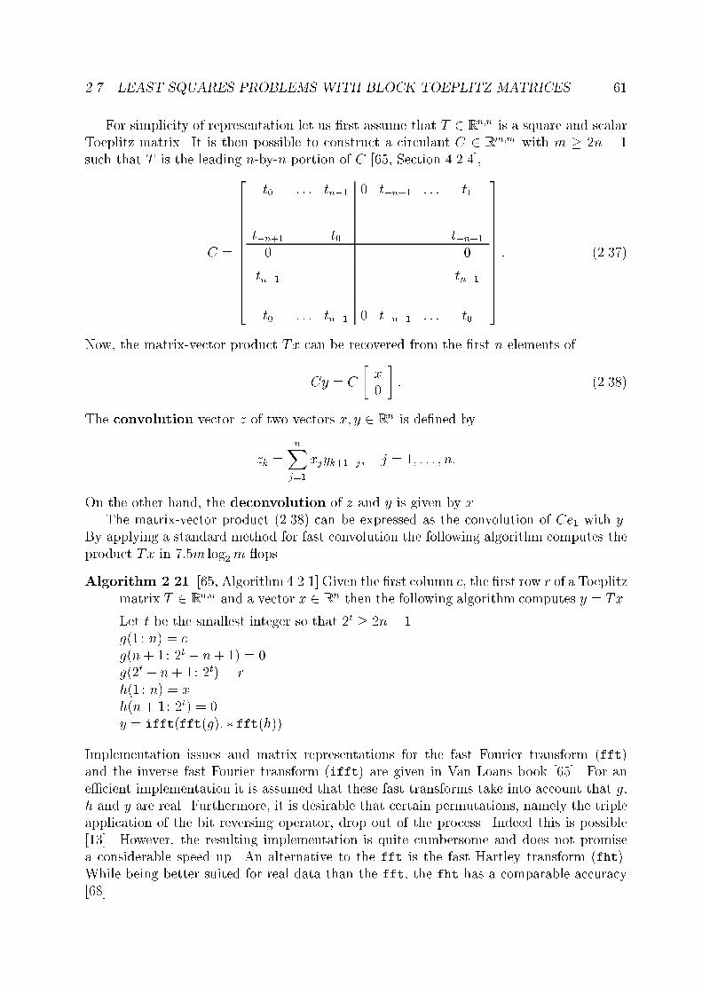
2.7. LEAST SQUARES PROBLEMS WITH BLOCK TOEPLITZ MATRICES 61For simplicity of representation let us �rst assume that T 2 Rn;n is a square and scalarToeplitz matrix. It is then possible to construct a circulant C 2 Rm;m with m � 2n � 1such that T is the leading n-by-n portion of C [65, Section 4.2.4],C =
2666666666664t0 : : : tn�1 0 t�n+1 : : : t1... . . . . . . . . . ...t�n+1 t0 . . . . . . t�n+10 0tn�1 . . . . . . . . . tn�1... . . . . . . ...t0 : : : tn�1 0 t�n+1 : : : t0
3777777777775 : (2.37)Now, the matrix-vector product Tx can be recovered from the �rst n elements ofCy = C � x0 � : (2.38)The convolution vector z of two vectors x; y 2 Rn is de�ned byzk = nXj=1 xjyk+1�j; j = 1; : : : ; n:On the other hand, the deconvolution of z and y is given by x.The matrix-vector product (2.38) can be expressed as the convolution of Ce1 with y.By applying a standard method for fast convolution the following algorithm computes theproduct Tx in 7:5m log2m ops.Algorithm 2.21 [65, Algorithm 4.2.1] Given the �rst column c, the �rst row r of a Toeplitzmatrix T 2 Rn;n and a vector x 2 Rn then the following algorithm computes y = Tx.Let t be the smallest integer so that 2t � 2n� 1.g(1 : n) = cg(n+ 1: 2t � n+ 1) = 0g(2t � n + 1: 2t) = rh(1 : n) = xh(n+ 1: 2t) = 0y = ifft(fft(g): � fft(h))Implementation issues and matrix representations for the fast Fourier transform (fft)and the inverse fast Fourier transform (ifft) are given in Van Loans book [65]. For ane�cient implementation it is assumed that these fast transforms take into account that g,h and y are real. Furthermore, it is desirable that certain permutations, namely the tripleapplication of the bit reversing operator, drop out of the process. Indeed this is possible[13]. However, the resulting implementation is quite cumbersome and does not promisea considerable speed up. An alternative to the fft is the fast Hartley transform (fht).While being better suited for real data than the fft, the fht has a comparable accuracy[68].

62 CHAPTER 2. MATRICES WITH BLOCK DISPLACEMENT STRUCTUREFor presenting fast transforming algorithms it is common to count the elements ofvectors and matrices starting from subscript 0 instead of 1. If not otherwise stated we usethis convention for the rest of this subsection.A vector ~x is said to be the Hartley transform of x 2 Rn if~xk = n�1Xj=0 �cos�2kj�n � + sin�2kj�n �� xj:Let Fn denote the DFT matrix, that is,Fn = �exp��2�ijn ��n�1i;j=0 :Fn is hermitian and scaled unitary. The Hartley transform stated in matrix-vector languageis ~x = Hnx := (Re(Fn)� Im(Fn))x:From Hn = HTn = nH�1n ;we see that the Hartley transform and its inverse are essentially the same. By de�ning�n = 1 + i2 In + 1� i2 Tn = 1 + i2 26664 1 . . . . . . 137775+ 1� i2 26664 1 0: : : 1: : : : : :0 1
37775we get Hn = �nFn:Here we stress the fact that �Fn = TnFn.Now we are ready to prove a fast convolution lemma for the Hartley transform.Lemma 2.22 Let z be the convolution vector of two real vectors x and y. Then2Hnz = ((In + Tn)Hnx): � (Hny) + (TnHnx): � ((In � Tn)Hny); (2.39)and for the deconvolutionHnz = [(Hnx): � ((In + Tn)Hny)� (TnHnx): � ((In � Tn)Hny)] (2.40):= [(Hny): � (Hny) + (TnHny): � (TnHny)]:Proof: The result (2.39) follows immediately from the equalityHnz = �nFnz = �n((Fnx): � (Fny))using the fact that permutations and summations can be distributed over the point-wise multiplication operator :�. (2.40) is proven analogously.

2.7. LEAST SQUARES PROBLEMS WITH BLOCK TOEPLITZ MATRICES 63It should be pointed out that at least (2.40) in Lemma 2.22 is not a novel idea, see e.g.[68].The fht algorithms are best described in terms of Kronecker products [65, Section4.3.11]. Using two vectors of length L=2,c = � cos(�) cos(2�) : : : cos((L� 1)�) �T ;s = � sin(�) sin(2�) : : : sin((L� 1)�) �T ;with � = �2�=L, let us de�ne the Hartley butter y matrix asBL = 2664 1 0 1 00 IL=2�1 0 diag(c)� diag(s)EL=2�11 0 �1 00 IL=2�1 0 �diag(c) + diag(s)EL=2�1 3775 ;where E = ��i;L=2�1�j�n�1i;j=0 denotes a permutation matrix of order L=2 � 1. An alreadymentioned permutation is the bit reversing operator Pn which is used in the followingalgorithm to compute the fht.Algorithm 2.23 If x 2 Rn and n = 2t, then the following algorithm overwrites x with itsHartley transform Hnx.x = Pnxfor l = 1: t doL = 2lx = (In=L BL)xendFrom(In=L B2t) � � � � � (In B1)Pn = Hn = HTn = P Tn (In BT1 ) : : : (In=L BT2t)we derive a transposed version of Algorithm 2.23 asAlgorithm 2.24 If x 2 Rn and n = 2t, then the following algorithm overwrites x with itsHartley transform Hnx.for l = 1: t doL = 2lx = (In=L BTL )xendx = PnxExploiting the sparsity of the matrices (In=L BL) resp. (In=L BTL ) shows that bothalgorithms require 2:5n log2 n ops. The implicit multiplication with Pn can take up to30 % of the execution time. With the following result we employ fast convolutions usingscrambled Hartley transforms.
64 CHAPTER 2. MATRICES WITH BLOCK DISPLACEMENT STRUCTURELemma 2.25 Let n = 2t, thenPnTnPn = Sn =: 1� E1 � E2 � � � � En=2: (2.41)Proof: By induction on t. The case t = 1 is trivial. For 2m = n > 1 the matrix Pnmay be represented as Pn = �n(Pm � Pm) = (Pm � Pm)�Tnwhere �Tn is the even-odd sort permutation, i.e.�Tnx = � x(0 : 2 : n� 2)x(1 : 2 : n� 1) � :The induction step is then given byPnTnPn = (Pm � Pm)�TnTn�n(Pm � Pm)= (Pm � Pm)(Tm � Em)(Pm � Pm)= (PmTmPm � PmEmPm) = (Sm � Em):Thus, the Hartley convolution identity (2.39) can be written as2PnHnz = (Pn(In + Tn)Hnx): � (PnHny) + (PnTnHnx): � (Pn(In � Tn)Hny)= ((In + Sn)PnHnx): � (PnHny) + (SnPnHnx): � ((In � Sn)PnHny);and the deconvolution (2.40) asPnHnZ = [(PnHnx): � ((In + Sn)PnHny)� (SnPnHnx): � ((In � Sn)PnHny)]:=[(PnHny): � (PnHny) + (SnPnHny): � (SnPnHny)]We �nally arrive at an e�cient algorithm for computing the Hartley convolution.Algorithm 2.26 If x; y 2 Rn and n = 2t, then the following algorithm overwrites x withthe convolution fdeconvolutiong of x and y:Update x = PnHnx and y = PnHny using Algorithm 2.24 without the last step.x(0 : 1) = x(0 : 1): � y(0 : 1) fx(0 : 1) = x(0 : 1):=y(0 : 1)gfor l = 1: t� 1 dos = 2lfor i = 0: s=2� 1 do� xs+ix2s�i�1 � = 12 � ys+i + y2s�i�1 ys+i � y2s�i�1�ys+i + y2s�i�1 ys+i + y2s�i�1 �f�1g � xs+ix2s�i�1 �endendUpdate x = HnPnx using Algorithm 2.23 without the �rst step.Scale x = x=n.
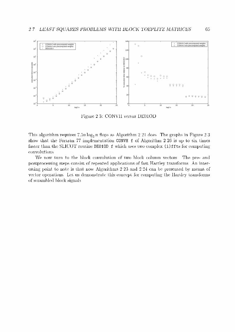
2.7. LEAST SQUARES PROBLEMS WITH BLOCK TOEPLITZ MATRICES 65
0 5 10 15 20 2510
−5
10−4
10−3
10−2
10−1
100
101
102
103
log2 n
exec
utio
n tim
e in
sec
onds
CONVH.f with precomputed weightsCONVH.f w/o precomputed weights DE01OD.f
0 5 10 15 20 250
20
40
60
80
100
120
140
log2 n
% e
xecu
tion
time
rela
tive
to D
E01
OD
.f
CONVH.f with precomputed weightsCONVH.f w/o precomputed weights
Figure 2.3: CONVH versus DE01OD.This algorithm requires 7:5n log2 n ops as Algorithm 2.21 does. The graphs in Figure 2.3show that the Fortran 77 implementation CONVH.f of Algorithm 2.26 is up to six timesfaster than the SLICOT routine DE01OD.f which uses two complex (i)ffts for computingconvolutions.We now turn to the block convolution of two block column vectors. The pre- andpostprocessing steps consist of repeated applications of fast Hartley transforms. An inter-esting point to note is that now Algorithms 2.23 and 2.24 can be presented by means ofvector operations. Let us demonstrate this concept for computing the Hartley transformsof scrambled block signals.

66 CHAPTER 2. MATRICES WITH BLOCK DISPLACEMENT STRUCTUREAlgorithm 2.27 This algorithm overwrites a given block column vector X 2 R2mk;l withthe kl Hartley transforms of the bit-reversed vectors X(s : k : 2mk; t), s = 1; : : : ; k,t = 1; : : : ; l.for t = 1: l dofor p = m� 1: � 1: 1� = ��=2pfor i = 0: 2�p�1 � 1 dofor j = 0: 2p�1 � 1 do2664 ~q1~q2~q3~q4 3775 = 2664 2p+1i+ j2p+1i + 2p + j2p+1i+ 2p � j2p+1i+ 2p+1 � j 3775 k:+ 2664 0: k � 10 : k � 10 : k � 10 : k � 1 3775y1 = X(~q1; t)�X(~q2; t)y2 = X(~q3; t)�X(~q4; t)X(~q1; t) = X(~q1; t) +X(~q2; t)X(~q3; t) = X(~q3; t) +X(~q4; t)� X(~q2; t) X(~q4; t) � = � y1 y2 � � cos j� sin j�sin j� � cos j� �endendendfor i = 0: n=2� 1 doy1 = X((2i+ 1)k : (2i+ 2)k � 1; t)X((2i+ 1)k : (2i+ 2)k � 1; t) = X(2ik : (2i+ 1)k � 1; t)� y1X(2ik : (2i+ 1)k � 1; t) = X(2ik : (2i+ 1)k � 1; t) + y1endendFor further implementation issues inspect the Fortran 77 routine TPMULT.f.As the consequence of a block formulation of Lemma 2.22 we get the following blockversion of Algorithm 2.26.Algorithm 2.28 If X 2 R2mk;l and Y 2 R2m l;p, then the following algorithm computesZ 2 R2mk;p as the block convolution of X and Y .Overwrite X with the bit-reversed Hartley transforms of X(s : k : 2mk � 1; t)for s = 0; : : : ; k � 1 and t = 0; : : : ; l � 1.Overwrite Y with the bit-reversed Hartley transforms of Y (s : l : 2ml � 1; t)for s = 0; : : : ; k � 1 and t = 0; : : : ; l � 1.Z0 = X0 � Y0Z1 = X1 � Y1

2.7. LEAST SQUARES PROBLEMS WITH BLOCK TOEPLITZ MATRICES 67for t = 1: m� 1 dos = 2tfor i = 0: s=2� 1 do� Zs+iZ2s�i�1 � = 12 � Xs+i +X2s�i�1 Xs+i �X2s�i�1�Xs+i +X2s�i�1 Xs+i +X2s�i�1 � � Ys+iY2s�i�1 �endendOverwrite Z with the Hartley transforms of the bit-reversed vectorsZ(s : k : 2mk � 1; t) for s = 0; : : : ; k � 1 and t = 0; : : : ; p� 1.Scale Z = Z=n.Let us consider the product T � B, where T is an m-by-n block Toeplitz matrix withk-by-l blocks and B is a general nl-by-r matrix. Our main goal is to minimize the numberof matrix-by-matrix multiplications involving a k-by-l matrix on the left hand side and anl-by-r matrix on the right hand side. In the following this number is denoted by #mm.For conventional multiplication algorithms, as implemented in the LAPACK subroutineDGEMM, we e�ectively have #mm(Multiplication) = mn. On the other hand, for Algorithm2.28, this value is given by max(2p+1 � 2; 1), where p is the smallest integer such that2p � m + n � 1. Figure 2.4 is a surface plot of the function #mm(Algorithm 2.28)- #mm(Multiplication) evaluated at di�erent points (m;n). We �lled areas where thisfunction takes large negative values with a dark color, and the small area where conventionalmultiplication is superior has a white color.
n
m
10 20 30 40 50 60 70 80 90 100
10
20
30
40
50
60
70
80
90
100Figure 2.4: Surface plot of #mm(Algorithm 2.28) � #mm(Multiplication).On modern computers, forming TB by conventional matrix-by-matrix multiplicationis a very e�cient and highly optimized process. It is doubtful whether Algorithm 2.28with its poor memory reference pattern and optimizer unfriendly structure can beat theperformance of the LAPACK subroutine DGEMM for modest matrix dimensions. Figure 2.5shows that convolution is always a good idea when dealing with point Toeplitz matrices.However, for small block sizes k; l > 1 and dimensions n;m straightforward multiplication

68 CHAPTER 2. MATRICES WITH BLOCK DISPLACEMENT STRUCTURE
0 200 400 600 800 1000 1200 1400 1600 1800 200010
−4
10−3
10−2
10−1
n × n Toeplitz matrix times vector
n
exec
utio
n tim
e in
sec
onds
by convolution by multiplication
0 100 200 300 400 500 60010
−3
10−2
10−1
100
101
102
20n × 20n Toeplitz matrix times 20n × 20 matrix
n
exec
utio
n tim
e in
sec
onds
by convolution by multiplication
Figure 2.5: Multiplication versus convolution for point and block Toeplitz matrices.is often the better advice. To be more speci�c, karl revealed after extensive performancetests that only if mn � max(2p+1 � 2; 1) andmnp � klr13(kl + lr + kr) � 950; (2.42)then block convolution should be preferred. Inequality (2.42) is certainly a crude rule ofthumb and should be adapted when using di�erent computer architectures.2.7.2 QR FactorizationTo illustrate the concept of the Schur reduction process for rank de�cient matrices let uscalculate a made-up example with Matlab.Example 2.29 Let T be a block Toeplitz matrix with k = l = 3 and m = n = 4, de�nedby its �rst block column and row,T (1 : 12; 1: 3)T = 24 1 1 1 1 1 1 1 1 1 1 1 22 2 2 2 2 2 2 2 2 0 1 23 3 3 3 3 3 3 3 3 1 0 0 35 ;T (1 : 3; 4: 12) = 24 1 2 3 1 2 3 0 1 11 2 3 1 2 3 1 2 11 2 3 1 2 3 1 1 1 35 :

2.7. LEAST SQUARES PROBLEMS WITH BLOCK TOEPLITZ MATRICES 69Then, by Theorem 2.20, a generator of T TT is given by2666666666666666664�9:0554 0 0 0 0 0 0 0 0 0 0 0�3:0921 2:3322 0 0 0 0 0 0 0 0 0 0�5:9633 1:9557 �1:2706 0 0 0 0 0 0 0 0 0�3:0921 1:4746 0:2541 1 1 1 �3:0921 1:4746 0:2541 1 1 2�6:1842 2:9492 0:5082 2 2 2 �6:1842 2:9492 0:5082 0 1 2�9:2762 4:4238 0:7623 3 3 3 �9:2762 4:4238 0:7623 1 0 0�3:0921 1:4746 0:2541 1 1 1 �3:0921 1:4746 0:2541 1 1 1�6:1842 2:9492 0:5082 2 2 2 �6:1842 2:9492 0:5082 2 2 2�9:2762 4:4238 0:7623 3 3 3 �9:2762 4:4238 0:7623 3 3 3�2:7608 1:4851 0:2894 0 1 1 �2:7608 1:4851 0:2894 1 1 1�5:5216 2:9701 0:5788 1 2 1 �5:5216 2:9701 0:5788 2 2 2�7:2885 4:4866 0:9741 1 1 1 �7:2885 4:4866 0:9741 3 3 3
3777777777777777775 ;where columns 1$ 2 and 2$ 3 of T are swapped. The �rst reduction step is free,the �rst 3 columns are moved 3 positions downward:2666666666664�9:0554 0 0 1 1 1 �3:0921 1:4746 0:2541 1 1 2�3:0921 2:3322 0 2 2 2 �6:1842 2:9492 0:5082 0 1 2�5:9633 1:9557 �1:2706 3 3 3 �9:2762 4:4238 0:7623 1 0 0�3:0921 1:4746 0:2541 1 1 1 �3:0921 1:4746 0:2541 1 1 1�6:1842 2:9492 0:5082 2 2 2 �6:1842 2:9492 0:5082 2 2 2�9:2762 4:4238 0:7623 3 3 3 �9:2762 4:4238 0:7623 3 3 3�3:0921 1:4746 0:2541 0 1 1 �2:7608 1:4851 0:2894 1 1 1�6:1842 2:9492 0:5082 1 2 1 �5:5216 2:9701 0:5788 2 2 2�9:2762 4:4238 0:7623 1 1 1 �7:2885 4:4866 0:9741 3 3 3
3777777777775 :Now, the semide�nite Cholesky downdating algorithm yields a swap of columns 4$ 6and the generator26666666666641:3416 0 0 0 0 0 : : ::8944 �2:3325 0 0 0 0 : : ::4472 �1:9549 1:2724 0 0 0 : : ::4472 �1:0974 1:0179 0 0 0 : : ::8944 �2:1948 2:0358 0 0 0 : : :1:3416 �3:2922 3:0537 0 0 0 : : ::4472 �1:0895 1:0444 0:5000 0:5774 0:5774 : : ::8944 �2:1791 2:0888 1 0:7887 �0:2113 : : :1:3416 �3:2450 3:2127 3 0 0 : : :: : : 0 0 0 0 0 0: : : �2:3325 0 0 0 0 0: : : �1:9549 1:2724 0 0 0 0: : : �1:0974 1:0179 0 0 0:4000 �0:2000: : : �2:1948 2:0358 0 0 0:8000 �0:4000: : : �3:2922 3:0537 0 0 1:2000 �0:6000: : : �1:0895 1:0444 0:0589 0:1557 0:4035 �0:1930: : : �2:1791 2:0888 0:1179 0:3114 0:8070 �0:3860: : : �3:2450 3:2127 0:3537 0:9342 1:2210 �0:5581
3777777777775 ;where columns 2; 3; 6 and 7 can be safely removed. Column 1 is moved 3 positionsdownwards. The next downdating swaps columns 7$ 9:2666664 �1:3416 0 0 0 �1:3416 0 0 0�0:8944 0 0 0 �0:8944 0 0 0�0:4472 0 0 0 �0:4472 0 0 0�0:4472 �0:3760 0:6259 0:6193 �0:4472 �0:0368 0:0162 0:1617�0:8944 �0:9300 0:8878 �0:1163 �0:8944 �0:0736 0:0324 0:3235�1:3416 �2:9681 0:3100 0:3067 �1:3416 �0:2208 0:0973 0:9705 3777775 :Hence, columns 1 and 4 can be removed. However, columns 2; : : : ; 4 and 6; : : : ; 9 mustbe preserved and their nonzero parts form the new generator. The last reduction stepyields the column swaps 10$ 12, 11$ 12 and24 2:8284 0 0 0 0 00:4714 0:8165 0 0 0 00:9428 0:4082 0:7071 0 0 0 35 :
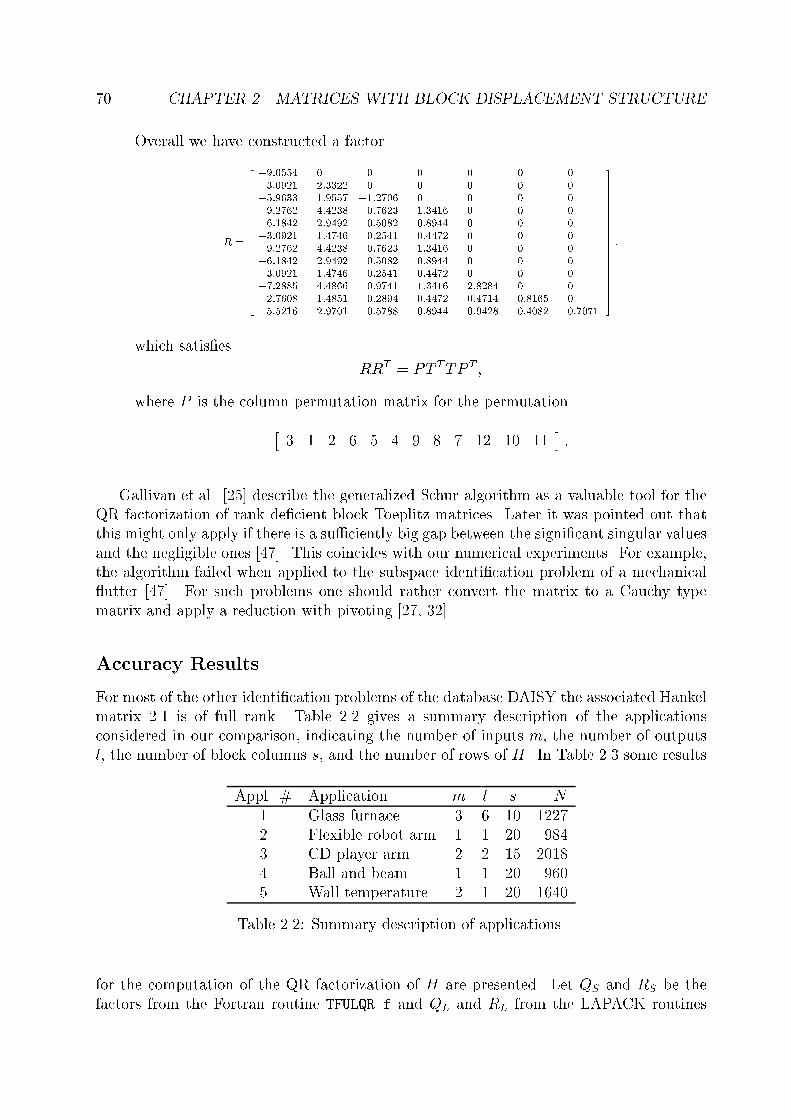
70 CHAPTER 2. MATRICES WITH BLOCK DISPLACEMENT STRUCTUREOverall we have constructed a factorR = 2666666666666666664
�9:0554 0 0 0 0 0 0�3:0921 2:3322 0 0 0 0 0�5:9633 1:9557 �1:2706 0 0 0 0�9:2762 4:4238 0:7623 1:3416 0 0 0�6:1842 2:9492 0:5082 0:8944 0 0 0�3:0921 1:4746 0:2541 0:4472 0 0 0�9:2762 4:4238 0:7623 1:3416 0 0 0�6:1842 2:9492 0:5082 0:8944 0 0 0�3:0921 1:4746 0:2541 0:4472 0 0 0�7:2885 4:4866 0:9741 1:3416 2:8284 0 0�2:7608 1:4851 0:2894 0:4472 0:4714 0:8165 0�5:5216 2:9701 0:5788 0:8944 0:9428 0:4082 0:70713777777777777777775 ;which satis�es RRT = PT TTP T ;where P is the column permutation matrix for the permutation� 3 1 2 6 5 4 9 8 7 12 10 11 � :Gallivan et.al. [25] describe the generalized Schur algorithm as a valuable tool for theQR factorization of rank de�cient block Toeplitz matrices. Later it was pointed out thatthis might only apply if there is a su�ciently big gap between the signi�cant singular valuesand the negligible ones [47]. This coincides with our numerical experiments. For example,the algorithm failed when applied to the subspace identi�cation problem of a mechanical utter [47]. For such problems one should rather convert the matrix to a Cauchy typematrix and apply a reduction with pivoting [27, 32].Accuracy ResultsFor most of the other identi�cation problems of the database DAISY the associated Hankelmatrix 2.1 is of full rank. Table 2.2 gives a summary description of the applicationsconsidered in our comparison, indicating the number of inputs m; the number of outputsl; the number of block columns s; and the number of rows of H. In Table 2.3 some resultsAppl. # Application m l s N1 Glass furnace 3 6 10 12272 Flexible robot arm 1 1 20 9843 CD player arm 2 2 15 20184 Ball and beam 1 1 20 9605 Wall temperature 2 1 20 1640Table 2.2: Summary description of applications.for the computation of the QR factorization of H are presented. Let QS and RS be thefactors from the Fortran routine TFULQR.f and QL and RL from the LAPACK routines

2.7. LEAST SQUARES PROBLEMS WITH BLOCK TOEPLITZ MATRICES 71DGEQRF.f and DORGQR.f. Then the following values are shown in the table,b? = kHTH � RT?R?k2=kHTHk2;r? = kH �Q?R?k2=kHk2;o? = kI �QT?Q?k2;c = kjRSj � jRLjk2=kjRLjk2:Appl. # bL rL oL1 1:15� 10�15 3:00� 10�15 7:02� 10�152 4:14� 10�15 7:04� 10�15 6:59� 10�153 1:37� 10�15 3:42� 10�15 7:04� 10�154 1:12� 10�15 2:18� 10�15 4:87� 10�155 2:43� 10�16 5:22� 10�16 6:24� 10�15Appl. # bS rS oS c1 2:10� 10�15 3:87� 10�15 1:00� 10�09 1:34� 10�112 2:66� 10�15 3:76� 10�15 3:40� 10�01 1:90� 10�033 8:94� 10�16 3:45� 10�15 1:05� 10�06 9:53� 10�094 2:15� 10�15 5:13� 10�15 5:63� 10�11 4:97� 10�135 1:44� 10�14 2:08� 10�14 3:94� 10�10 6:48� 10�13Table 2.3: Comparative results for computing the QR factorization.Since the orthogonal factor is implicitly obtained from the formula H(RTR)�1RT thedisappointing results for the values oS and rS are not surprising. Computing the orthogonalfactor by the Schur algorithm is often pointless when no reorthogonalization schemes areapplied afterwards. The extreme case is represented by the robot arm (application #2)due to the fact that the involved Hankel matrix has a condition number close to 1=peps.On the other hand, the factor RS has a low relative backward error which is especiallyuseful when solving normal equations [57].Performance ResultsAlthough the existence of a high performance Toeplitz toolbox, including QR factoriza-tions, was announced in [25]; it has not appeared yet. The only benchmark results notextrapolated from Matlab routines or op counts were given in [31]. However, it shouldbe mentioned that [31] uses completely di�erent blocking techniques. Therefore, withoutaccuracy results, it is hard to tell the value of the algorithms. Additionally, the codes arenot released for public. For k = l = 5 and m = n = 200 it is stated in [31, page 59]that the implemented algorithm "performed about 10 times faster compared to SGEQRF"when computing the R factor. karl required 5:90 seconds for the call of the LAPACKroutine DGEQRF.f applied on the explicitly constructed block Toeplitz matrix. It took only0:51 seconds when using TFULQR.f. For k = l = 50 and m = n = 8 the slow and the fast

72 CHAPTER 2. MATRICES WITH BLOCK DISPLACEMENT STRUCTUREalgorithms require approximately the same time in [31, Figure 8.2]. In this case a call ofDGEQRF.f yields 0:42 seconds execution time and TFULQR.f 0:37 seconds.To provide information about the in uence of the four di�erent dimensions k; l;m andn on the execution times we summarize the most signi�cant performance results in Table2.4. TFULQR.f DGEQRF.f/DORGQR.fblocked k l m n R Q R Qn/a 1 1 4096 2048 0:71 2:73 355:00 355:02n/a 1 1 2048 4096 1:98 1:40 339:50 127:29yes 4 4 1024 512 1:99 8:47 355:00 355:02yes 4 4 512 1024 5:70 4:18 339:50 127:29yes 16 16 256 128 4:81 29:56 355:00 355:02yes 16 16 128 256 13:84 13:95 339:50 127:29yes 64 64 64 32 20:09 164:64 355:00 355:02no 64 64 64 32 48:77 210:09 355:00 355:02yes 64 64 32 64 53:58 62:24 339:50 127:29no 64 64 32 64 134:49 100:23 339:50 127:29yes 128 32 32 32 6:31 44:98 110:21 110:09no 128 32 32 32 17:60 154:37 110:21 110:09yes 32 128 32 32 26:81 8:15 76:88 10:53no 32 128 32 32 69:43 16:07 76:88 10:53yes 512 512 4 4 109:36 117:96 127:16 128:10no 512 512 4 4 271:85 623:21 127:16 128:10Table 2.4: Execution times in seconds for the QR factorization using TFULQR.f andDGEQRF.f.2.7.3 Banded QR factorizationLet T have only ml lower and nu upper nonzero block bands, that is Ti = Tj = 0 fori < �ml and j > nu. If one is only interested in computing R, then during the applicationof the generalized Schur algorithm the generator has at most nu+ml+1 nonzero blocks ineach column. The Fortran 77 routine TPQRB.f exploits this sparsity and thus requires lessexecution time and memory space. Both �gures are improved by an approximate factor ofn=(ml + nu + 1).2.7.4 Direct Least Squares SolutionFor over- or underdetermined systems we want to �nd a vector x such that Tx is in a sensethe "best" approximation to b. A choice motivated for statistical reasons [9, Section 1.1]is typically minx kTx� bk2 (2.43)
2.7. LEAST SQUARES PROBLEMS WITH BLOCK TOEPLITZ MATRICES 73for overdetermined and minkyk2; T Tx = bkTx� bk2: (2.44)for underdetermined systems. Here, T still denotes an mk-by-nl block Toeplitz matrix butfrom now on we assume that T is of full column rank. This assumption particularly impliesthat T TT is positive de�nite.In a recent article Park and Eld�en [57] discuss several existing and new approaches forsolving linear least squares problems involving Toeplitz matrices. They propose to re�nethe obtained solution from a fast solver by using corrected seminormal equations. It mustbe noted that for ill-conditioned T TT the Schur algorithm is not useful if not combinedwith such correction steps afterwards. And sometimes even this strategy is not successful.However, this rather subtle question goes beyond the scope of this treatment.One interesting fact not mentioned in [57] is that a direct solution of the normal equa-tions T TTx = T T b;being formally equivalent to the solution of (2.43), can be computed without saving Rfrom a QR factorization. Although memory is nowadays cheap, it still makes a di�erencewhether an algorithm requires O(l2n2) or just O(ln) additional memory.Similar to the direct solution of linear systems (Remark 2.19, the derived method isnumerically the same as computing the Cholesky factors R and L such thatT TT = RTR; (T TT )�1 = LTL;by the generalized Schur algorithm and solving the equationRx = LT T bby blocked backward substitution.Our generalized Schur algorithm is built on the embedding� T TT �T T bI 0 � ; (2.45)where x is the Schur complement of T TT .The solution for the underdetermined system (2.44) is given byx = T (T TT )�1b;which may be represented as the Schur complement of T TT in� T TT �bT 0 � : (2.46)Both embeddings clearly have low displacement ranks and analogous to Theorem 2.20 gen-erators for (2.45) and (2.46) can be easily constructed as shown in the following corollary.

74 CHAPTER 2. MATRICES WITH BLOCK DISPLACEMENT STRUCTURECorollary 2.30 Given the QR factorization of the �rst block column of a block Toeplitzmatrix T 2 Rmk;nl with full rank,264 T0...T�m+1 375 = 264 C0...C�m+1 375R0; (2.47)where R0 is upper triangular, and264 S0...Sn�1 375 = T T 264 C0...C�m+1 375 ; 264 L0...Ln�1 375 = T T b: (2.48)Then generator pairs for (2.45) and (2.46) are given byX1 =
2666666666664S0 0 0 0 L0S1 T T1 S1 T T�m+1 L1... ... ... ... ...Sn�1 T Tn�1 Sn�1 T Tn�m�1 Ln�1R�10 0 R�10 0 00 0 0 0 0... ... ... ... ...0 0 0 0 0
3777777777775 ;Y1 = 2666664 S0 0 0 0 0S1 T T1 S1 T T�m+1 0... ... ... ... ...Sn�1 T Tn�1 Sn�1 T Tn�m�1 00 0 0 0 �I
3777775andX2 =
2666666666664S0 0 0 0 B0S1 T T1 S1 T T�m+1 B1... ... ... ... ...Sn�1 T Tn�1 Sn�1 T Tn�m�1 Bn�1C0 Ik C0 0 0C1 0 C1 0 0... ... ... ... ...Cm�1 0 Cm�1 0 0
3777777777775 ; Y2 = Y1;respectively.Similar to Section 2.6.3 the solution of (2.43) or (2.44) can be recovered after theapplication of n� 1 block Schur steps to one of the generators presented in Corollary 2.30.

2.8. TOEPLITZ PLUS HANKEL SYSTEMS 752.8 Toeplitz plus Hankel systemsThe QR factorization of Toeplitz plus Hankel matrices plays a role in applications likemoving average processes [74]. This section shall rather lay a foundation stone for achievingsuch factorizations than giving a complete treatment of this complex issue.Of interest is now a displacement equation for ATA where A = T +H 2 Rn;n andT = 26664 t0 t1 : : : tn�1t�1 . . . . . . ...... . . . . . . t1t�n+1 t�1 t037775 ; H = 26664 hn�1 : : : h1 h0... : : : : : : h�1h1 : : : : : : ...h0 h�1 h�n+1
37775 :Unfortunately, the right shift matrix Z does not give low rank in this case. One has to useZ + ZT as the displacement operator and consider the transformationr(ATA) = (Z + ZT )ATA� ATA(Z + ZT ): (2.49)The matrix r(ATA) is skew-symmetric and hopefully of low rank. Similar to (2.3) we callG 2 Rn;2� a generator of rATA if G satis�esrATA = G � 0 I��I� 0 �| {z }J GT :Recently, Heinig and Olshevsky [33] proposed a new algorithm for displacement equa-tions of the form (2.49). A di�erent version, which exploits the symmetries in (2.49), isgiven by the following algorithm.Algorithm 2.31 Given a generator G 2 Rn;2� forrATA this algorithms computes a lowertriangular factor L such that LLT = ATA.r = eT1ATAF = Z + ZTfor k = 1: n� 1 dox = r(1); l = r=pxL(k : n; n) = lr2 = ((F � F11In�k+1)r �GJG(1; : )T )=F12r = r2(2 : n� k + 1)� r(2)=px l(2 : n� k + 1)F = F (2 : n� k + 1; 2: n� k + 1)� F (2; 3)=px l(2 : n� k + 1)eT1G = G� 1=px lG(1; : )G = G(2 : n� k + 1; : )endLnn = sqrt(r)The above procedure is implemented as the Matlab routine tphqr.m. An analyticexpression for G is given by the following lemma.

76 CHAPTER 2. MATRICES WITH BLOCK DISPLACEMENT STRUCTURELemma 2.32 Given the Toeplitz matrix T , the Hankel matrix H, A = (T +H)T (T +H)and c = ZAe1 + ZTAe1 � Ae2; d = ZAen + ZTAen � Aen�1:Then a generator G for the displacement rATA, as de�ned in (2.49), is given by266666664c1 0 0 0 1 0 0 0c2 d2 t2 + hn�1 t�n+1 + h�2 0 0 t1 + hn�2 t�n+2 + h�1... ... t3 + hn�2 t�n+2 + h�3 ... ... t2 + hn�3 t�n+3 + h�2... ... ... ... ... ... ... ...cn�1 dn�1 tn�1 + h2 t�2 + h�n+1 0 0 tn�2 + h1 t�1 + h�ncn dn 0 0 0 1 0 0
377777775 :Proof: Note that only the vectors c and d contribute to the borders of the productGGT . It readily follows thatrATAGGT = 24 1 n�2 11 0 0 0n�2 0 ? 01 0 0 035:The inner region of rATA, denoted by the star, is the annoying part of the proof.Since Tei = 264 ti�1...t�n+i 375 ; Hei = 264 hn�i...hi�1 375 ;we have for i; j > 2 thateTi (rATA)ej = eTi (Z + ZT )ATAej � eTi ATA(Z + ZT )ej= (Aei�1 + Aei+1)TAej � (Aei)T (Aej�1 + Aej+1)= (ZTei + t�n+i�1en + ZHei + hn�i+1e1+ZTTei + tie1 + ZTHei + hien)T (T +H)ej�eTi (T +H)T (ZTej + t�n+j�1en + ZHej + hn�j+1e1+ZTTej + tje1 + ZTHej + hjen)= (t�n+i�1en + hn�i+1e1 + tie1 + hien)T (T +H)ej�eTi (T +H)T (t�n+j�1en + hn�j+1e1 + tje1 + hjen);completing the proof.Recently, Benner et.al. [5] presented an algorithm for computing Cholesky-like factor-izations of skew-symmetric matrices. An interesting question, arising from this section, iswhether Algorithm (2.31) can be presented in terms of downdating/updating such factor-izations.

ConclusionsWe discuss performance and accuracy aspects of the periodic QZ algorithm. Blockedformulations of the involved orthogonal transformations increase the data locality andthus address the �rst task. For the sake of reliability the proposed implementation includesbalancing, implicit methods for computing shifts and carefully chosen de ation strategies.It is also shown how other QZ like algorithms could bene�t from these improvements.The second part describes several variants of the classical Schur algorithm which weimplemented for the computation of various factorizations of Toeplitz and block Toeplitzmatrices. The considered problems always implicitly rely on the Cholesky factorizationof semide�nite matrices, for which the Schur algorithm has been shown to be numericallyreliable. Numerical results substantiating this claims are included.Ready to use FORTRAN 77 routines complement this work.
77

78 CONCLUSIONS

Bibliography[1] G. S. Ammar, W. B. Gragg, and L. Reichel. On the eigenproblem for orthogonalmatrices. In Proc. IEEE Confrence on Decision and Control, pages 1963{1966, 1985.[2] E. Anderson, Z. Bai, C. Bischof, J. Demmel, J. Dongarra, J. Du Croz, A. Greenbaum,S. Hammarling, A. McKenney, S. Ostrouchov, and D. Sorensen. LAPACK Users'Guide. SIAM, Philadelphia, PA, second edition, 1994.[3] P. Benner and R. Byers. An arithmetic for matrix pencils. In A. Beghi, L. Finesso,and G. Picci, editors, Theory of Networks and Systems, pages 573{576. Il Poligrafo,Padova, Italy, 1998.[4] P. Benner and R. Byers. Evaluating products of matrix pencils and collapsing ma-trix products. Mathematics research reports 99-12-01, Department of Mathematics,University of Kansas, 2000.[5] P. Benner, R. Byers, H. Fassbender, V. Mehrmann, and D. Watkins. Cholesky-likefactorizations of skew-symmetric matrices. Electron. Trans. Numer. Anal., 11:85{93,2000.[6] P. Benner, R. Byers, V. Mehrmann, and H. Xu. Numerical computation of de at-ing subspaces of embedded Hamiltonian pencils. Preprint SFB393/99-15, Sonder-forschungsbereich 393, `Numerische Simulation auf massiv parallelen Rechnern', 1999.[7] P. Benner, V. Mehrmann, V. Sima, S. Van Hu�el, and A. Varga. SLICOT|a sub-routine library in systems and control theory. In Applied and computational control,signals, and circuits, Vol. 1, pages 499{539. Birkh�auser Boston, Boston, MA, 1999.[8] P. Benner, V. Mehrmann, and H. Xu. Perturbation analysis for the eigenvalue problemof a formal product of matrices. Berichte aus der Technomathematik 00-01, Fachbere-ich Mathematik und Informatik, Univ. Bremen, 2000.[9] �A. Bj�orck. Numerical methods for least squares problems. Society for Industrial andApplied Mathematics (SIAM), Philadelphia, PA, 1996.[10] A. Bojanczyk, G. H. Golub, and P. Van Dooren. The periodic Schur decomposition;algorithm and applications. In Proc. SPIE Conference, volume 1770, pages 31{42,1992.[11] A. W. Boja�nczyk and A. O. Steinhardt. Stabilized hyperbolic Householder transfor-mations. IEEE Trans. Acoust. Speech Signal Process., 37(8):1286{1288, 1989.79
80 BIBLIOGRAPHY[12] D. L. Boley. The algebraic structure of pencils and block Toeplitz matrices. LinearAlgebra Appl., 279(1-3):255{279, 1998.[13] W. L. Briggs. Further symmetries of in-place FFTs. SIAM J. Sci. Statist. Comput.,8(4):644{654, 1987.[14] James R. Bunch. Stability of methods for solving Toeplitz systems of equations. SIAMJ. Sci. Statist. Comput., 6(2):349{364, 1985.[15] P. Businger and G. H. Golub. Handbook series linear algebra. Linear least squaressolutions by Householder transformations. Numer. Math., 7:269{276, 1965.[16] R. Byers and N. Rhee. Cyclic Schur and Hessenberg-Schur numerical methods forsolving periodic Lyapunov and Sylvester equations. Technical report, University ofMissouri at Kansas City, 1995.[17] Ralph Byers, Chunyang He, and Volker Mehrmann. Where is the nearest non-regularpencil? Linear Algebra Appl., 285(1-3):81{105, 1998.[18] R. H. Chan and P. T. P. Tang. Fast band-Toeplitz preconditioners for HermitianToeplitz systems. SIAM J. Sci. Comput., 15(1):164{171, 1994.[19] J. Chun, T. Kailath, and V. Roychowdhury. Systolic array for solving Toeplitz systemsof equations, pages 547{560. Oxford and IBH Publishing Co., India, 1990.[20] G. Cybenko and M. Berry. Hyperbolic Householder algorithms for factoring structuredmatrices. SIAM J. Matrix Anal. Appl., 11(4):499{520, 1990.[21] K. Dackland and B. K�agstr�om. Blocked algorithms and software for reduction of aregular matrix pair to generalized Schur form. ACM Trans. Math. Software, 25(4):425{454, 1999.[22] B. De Moor and P. Van Dooren. Generalizations of the singular value and QR-decompositions. SIAM J. Matrix Anal. Appl., 13(4):993{1014, 1992.[23] J. J. Dongarra, J. R. Bunch, C. B. Moler, and G. W. Stewart. LINPACK Users'Guide. SIAM, Philadelphia, PA, USA, 1979.[24] K. V. Fernando and S. Hammarling. A product induced singular value decomposi-tion (�SVD) for two matrices and balanced realization. In Linear algebra in signals,systems, and control (Boston, MA, 1986), pages 128{140. SIAM, Philadelphia, PA,1988.[25] K. A. Gallivan, S. Thirumala, P. Van Dooren, and V. Vermaut. High performance al-gorithms for Toeplitz and block Toeplitz matrices. Linear Algebra Appl., 241-243:343{388, 1996.[26] J. D. Gardiner, A. J. Laub, J. J. Amato, and C. B. Moler. Solution of the Sylvestermatrix equation AXBT + CXDT = E. ACM Trans. Math. Software, 18(2):223{231,1992.
BIBLIOGRAPHY 81[27] I. Gohberg, T. Kailath, and V. Olshevsky. Fast Gaussian elimination with partialpivoting for matrices with displacement structure. Math. Comp., 64(212):1557{1576,1995.[28] I. Gohberg and A. Semencul. On the inversion of �nite Toeplitz matrices and theircontinuous analogs. Mat. Issled., 2:201{233, 1972.[29] G. Golub and W. Kahan. Calculating the singular values and pseudo-inverse of amatrix. J. Soc. Indust. Appl. Math. Ser. B Numer. Anal., 2:205{224, 1965.[30] G. H. Golub and C. F. Van Loan. Matrix Computations. Johns Hopkins UniversityPress, Baltimore, third edition, 1996.[31] B. Hallinger. Block algorithms for downdating and for factorizations of Toeplitz ma-trices. Master's thesis, Department of Mathematics, Link�oping University, 1996.[32] G. Heinig. Inversion of generalized Cauchy matrices and other classes of structuredmatrices. In Linear algebra for signal processing (Minneapolis, MN, 1992), pages63{81. Springer, New York, 1995.[33] G. Heinig and V. Olshevsky. The Schur algorithm for matrices with Hessenberg dis-placement structure. Contemporary mathematics, AMS publications, 2001. to appear.[34] G. Heinig and K. Rost. Algebraic methods for Toeplitz-like Matrices and Operators.Akademie-Verlag, Berlin and Birkh�auser, 1984.[35] J. J. Hench and A. J. Laub. Numerical solution of the discrete-time periodic Riccatiequation. IEEE Trans. Automat. Control, 39(6):1197{1210, 1994.[36] N. J. Higham. Analysis of the Cholesky decomposition of a semi-de�nite matrix. InReliable numerical computation, pages 161{185. Oxford Univ. Press, New York, 1990.[37] N. J. Higham. Accuracy and stability of numerical algorithms. Society for Industrialand Applied Mathematics (SIAM), Philadelphia, PA, 1996.[38] T. Kailath. Linear Systems. Prentice-Hall, Englewood Cli�s, NJ, 1980.[39] T. Kailath and A. H. Sayed. Fast Reliable Algorithms for Matrices with Structure.SIAM, Philadelphia, 1999.[40] T. Kailath and A.H. Sayed. Displacement structure: theory and applications. SIAMReview, 37:297{386, 1995.[41] T. Kailath, A. Vieira, and M. Morf. Displacement ranks of matrices and linear equa-tions. J. Math. Anal. Appl., 68:395{407, 1979.[42] L. Kaufman. Some thoughts on theQZ algorithm for solving the generalized eigenvalueproblem. ACM Trans. Math. Software, 3(1):65{75, 1977.[43] D. Kressner and P. Van Dooren. Factorizations and linear system solvers for matriceswith Toeplitz structure. SLICOT working note 2000-2, WGS, 2000.

82 BIBLIOGRAPHY[44] W.-W. Lin, P. Van Dooren, and Q.-F. Xu. Characterizations of periodic invariantsubspaces. in preparation.[45] W.-W. Lin and J.-G. Sun. Perturbation analysis of eigenvalue and eigenvectors ofperiodic matrix pairs. Report UMINF 00.02, Dept. of Computing Science, Ume�aUniversity, 2000.[46] K. Lust. Continuation and bifurcation analysis of periodic solutions of partial di�er-ential equations. In Continuation methods in uid dynamics (Aussois, 1998), pages191{202. Vieweg, Braunschweig, 2000.[47] N. Mastronardi, D. Kressner, V. Sima, S. Van Hu�el, and P. Van Dooren. Fast algo-rithms for subspace state-space system identi�cation via exploitation of the displace-ment structure. Journal of Computational and Applied Mathematics, Special issue on'Advanced numerical methods for mathematical modeling', 2001. accepted.[48] MATLAB User's Guide. The MathWorks, Inc., Natick, MA, USA, 1992.[49] R. Mayo and E. S. Quintana. Periodic Schur reduction package (version 0.1), 1999.[50] M. Miranda and P. Tilli. Asymptotic spectra of Hermitian block Toeplitz matricesand preconditioning results. SIAM J. Matrix Anal. Appl., 21(3):867{881, 2000.[51] C. B. Moler and G. W. Stewart. An algorithm for generalized matrix eigenvalueproblems. SIAM J. Numer. Anal., 10:241{256, 1973. Collection of articles dedicatedto the memory of George E. Forsythe.[52] B. De Moor. On the structure of generalized SVD and QR. SIAM Matrix Anal. Appl.,15:347{358, 1994.[53] B. De Moor, P. De Gersem, B. De Schutter, and W. Favoreel. DAISY: A database foridenti�cation of systems. Journal A (Benelux publication of the Belgian Federation ofAutomatic Control), 38(3):4{5, 1997.[54] B. De Moor, P. Van Overschee, and W. Favoreel. Numerical Algorithms for SubspaceState-Space System Identi�cation { An Overview, volume 1, chapter 6. Birkh�auser,Boston, 1999.[55] B. De Moor and H. Zha. A tree of generalizations of the ordinary singular valuedecomposition. Linear Algebra Appl., 147:469{500, 1991. special issue on CanonicalForms of Matrices.[56] S. Oliveira and D. E. Stewart. Exponential splittings of products of matrices andaccurately computing singular values of long products. In Proceedings of the Interna-tional Workshop on Accurate Solution of Eigenvalue Problems (University Park, PA,1998), volume 309:1-3, pages 175{190, 2000.[57] H. Park and L. Eld�en. Schur-type methods for solving least squares problems withToeplitz structure. SIAM J. Sci. Comput., 22(2):406{430, 2000.

BIBLIOGRAPHY 83[58] I. Schur. �Uber Potenzreihen die im Inneren des Einheitskreises beschr�ankt sind. J.Reine Angew. Math., 147:205{232, 1917.[59] V. Sima. Cholesky or QR factorization for data compression in subspace{based identi-�cation? In Proceedings Second NICONET Workshop, Paris{Versailles, Dec. 3, pages75{80, 1999.[60] J. Sreedhar and P. Van Dooren. On �nding stabilizing state feedback gains for adiscrete-time periodic system. In American Control Conf., pages 1167{1168, 1994.[61] J. Sreedhar and P. Van Dooren. Pole placement via the periodic Schur decomposition.In Proceedings Amer. Contr. Conf., pages 1563{1567, 1993.[62] J. Sreedhar and P. Van Dooren. A Schur approach for solving some periodic matrixequations. In U. Helmke, R. Mennicken, and J. Saurer, editors, Systems and Networks: Mathematical Theory and Applications, volume 77, pages 339{362. Akademie Verlag,Berlin, 1994.[63] M. Stewart and P. Van Dooren. Stability issues in the factorization of structuredmatrices. SIAM J. Matrix Anal. Appl., 18:104{118, 1997.[64] C. F. Van Loan. A general matrix eigenvalue algorithm. SIAM J. Numer. Anal.,12(6):819{834, 1975.[65] C. F. Van Loan. Computational frameworks for the fast Fourier transform. Societyfor Industrial and Applied Mathematics (SIAM), Philadelphia, PA, 1992.[66] P. Van Overschee and B. De Moor. Subspace identi�cation for linear systems. KluwerAcademic Publishers, Boston, MA, 1996. Theory|implementation|applications,With 1 IBM-PC oppy disk (3.5 inch; HD).[67] A. Varga. Periodic Lyapunov equations: some applications and new algorithms. In-ternat. J. Control, 67(1):69{87, 1997.[68] V. Vesel�y. Fast algorithms of Fourier and Hartley transform and their implementationin MATLAB. In Summer School DATASTAT 97, Proceedings (Hod�unka), pages 185{232, Brno, 1998. Masaryk Univ.[69] R. C. Ward. The combination shift QZ algorithm. SIAM J. Numer. Anal., 12(6):835{853, 1975.[70] R. C. Ward. Balancing the generalized eigenvalue problem. SIAM J. Sci. Statist.Comput., 2(2):141{152, 1981.[71] D. S. Watkins. Performance of the QZ algorithm in the presence of in�nite eigenvalues.SIAM J. Matrix Anal. Appl., 22(2):364{375, 2000.[72] David S. Watkins. The transmission of shifts and shift blurring in the QR algorithm.In Proceedings of the Fourth Conference of the International Linear Algebra Society(Rotterdam, 1994), volume 241/243, pages 877{896, 1996.

84 BIBLIOGRAPHY[73] J. H. Wilkinson. The algebraic eigenvalue problem. Clarendon Press, Oxford, 1965.[74] G. Wilson. Factorization of the covariance generating function of a pure movingaverage process. SIAM J. Numer. Anal., 6:1{7, 1969.[75] The Working Group on Software: WGS, Available from http://www.win.tue.nl/wgs/reports.html. SLICOT Implementation and Documentation Standards 2.1,1996. WGS-report 96-1.

Appendix AAn Arithmetic for Matrix PencilsAn arithmetic for k-matrix pencils can be found in Benner and Byers [3]. The representa-tion of formal matrix products with inverses as linear relations on Rn�Rn is an alternativeway to avoid the hobbling use of inverses involving singular matrices.In this appendix, the main concept is reviewed.De�nition A.1 A linear relation is a set of ordered pairs of the form(EnA) := f(x; y) 2 Rn � Rn j Ey = Axg; (A.1)for some matrices A 2 Rn�n and E 2 Rn�n .Note that in the case of a regular matrix E, the relation (A.1) can be considered as alinear transformation representated by the matrix E�1A. Though every linear relation isclearly a vector subspace of R2n the converse is not true. For example the trivial subspacef(0; 0)g � R2n cannot be represented by a linear relation in the sense of De�nition A.1.Furthermore, the representation of relations is not unique; we have the following lemma.Lemma A.2 (EnA) = ( ~En ~A) (A.2)holds if and only if there exists a nonsingular matrix M such that ~E = ME and~A =MA.Proof: If ~E =ME and ~A =MA, then the set equality (A.2) trivially holds.On the other hand, if (EnA) = ( ~En ~A) then kernel E = kernel ~E which implies theexistence of a matrix V2, with V T2 V2 = I, such that EV2 = ~EV2 = 0. Furthermore,we can �nd an orthogonal matrix V = � V1 V2 � such that EV1 and ~EV1 have fullcolumn rank. Hence, there exist nonsingular matrices P and Q withE = P � Ik 00 0 �V; ~E = Q � Ik 00 0 �V:Then, (A.2) is equivalent to the condition that� Ik 00 0 � � y1y2 � = Bz }| {P�1A � x1x2 � , � Ik 00 0 � � y1y2 � = ~Bz }| {Q�1 ~A � x1x2 �85

86 APPENDIX A. AN ARITHMETIC FOR MATRIX PENCILSholds for all x1; y1 2 Rk and x2; y2 2 Rn�k+1 . By partitioning B = � B11 B12B21 B22 �analogously, this equivalence is transformed toB11x1 +B12x2 = y1B21x1 +B22x2 = 0 , ~B11x1 + ~B12x2 = y1~B21x1 + ~B22x2 = 0 ;which yieldskernel � ~B21 ~B22 � = kernel � B21 B22 � � kernel � B11 � ~B11 B12 � ~B12 � :Thus, there exists a nonsingular matrix T and a (possibly singular) matrix S suchthat ~B = � Ik S0 T �B: Finally, settingM = Q � Ik S0 T �P�1completes the proof.De�nition A.3 If (E1nA1) and (E2nA2) are linear relations then the composite or prod-uct relation is de�ned by(E2nA2)(E1nA1) = �(x; z) 2 Rn � Rn ����9y 2 Rn : (y; z) 2 (E2nA2)(x; y) 2 (E1nA1) � : (A.3)Note that if E1 and E2 are nonsingular then (A.3) corresponds to the product E�12 A2E�11 A1.Some simple rules1. (E2nA2)(InnA1) = (E2nA2A1)2. (E2nIn)(E1nA1) = (E1E2nA1)3. (EnA) = (EDEnA � EDA + EDEA), where ED denotes the Drazin inverse ofE.4. (E1nA1) = (E2nA2) , (A1nE1) = (A2nE1)5. If kernel � ~A2 ~E1 � = range � �E1A2 � then (E2nA2)(E1nA1) = ( ~E1E2n ~A2A1):Proof: Rules 1-4 are straightforward, for the proof of 5 see [3].Collapsing For periodic eigenvalue problems the notion of collapsing as described in [4]is of theoretical and practical interest. Given a composition of several linear relations(E1nA1)(E2nA2) : : : (EknAk) (A.4)we can always determine two matrices E and A such that the relation (EnA) is equal to(A.4). Using generalized SVD algorithms, the so called collapsing procedure is proven tobe stable for k = 2.It now follows that for a k-matrix pencil (A; s) it is possible, without computing the pe-riodic Schur form, to �nd two matrices E and A of the same order such that the generalizedeigenvalue problem A� �E and (A; s) have the same eigenvalues.

Appendix BPeriodic QZ CodesAll routines and their depending subroutines described in thisthesis are available as Matlab or Fortran 77 �les under the URLhttp://www.tu-chemnitz.de/~dkr/diplom/.Here, for the readers convenience, only calling sequences andinline-documentations of the main routines are listed. The doc-umentation of the subroutine PGGBRD.f is ommitted since it isvirtually equivalent with that of PGGHRD.f.B.1 Hessenberg ReductionThe Fortran 77 subroutine PGGHRD.fSUBROUTINE PGGHRD( COMPQ, QIND, TRIU, K, N, H, ILO, IHI, S, A,$ LDA1, LDA2, Q, LDQ1, LDQ2, IWORK, DWORK,$ LDWORK, IWORK, LIWORK, INFO )CC PURPOSECC To reduce the general productCC S(1) S(2) S(K)C A(:,:,1) * A(:,:,2) * ... * A(:,:,K)CC to upper Hessenberg-triangular form.C A is N-by-N-by-K and S is the signatureC array with values 1 or -1. The H-th matrix of A is reduced toC upper Hessenberg form while the other matrices are triangularized.C Unblocked version.CC If COMPQ = 'V' or COMPZ = 'I', then the orthogonal factors areC computed and stored in the array Q so that for S(I) = 1,CC TC Q(:,:,I)(in) A(:,:,I) Q(:,:,MOD(I,K)+1)(in)C T (1)C = Q(:,:,I)(out) A(:,:,I) Q(:,:,MOD(I,K)+1)(out),CC and for S(I) = -1,CC TC Q(:,:,MOD(I,K)+1)(in) A(:,:,I) Q(:,:,I)(in)C T (2)C = Q(:,:,MOD(I,K)+1)(out) A(:,:,I) Q(:,:,I)(out).CC A partial generation of the orthogonal factors can be realizedC via the array QIND.CC ARGUMENTSCC Mode ParametersCC COMPQ (input) CHARACTER*1C = 'N': do not modify Q.C = 'V': modify the array Q by the orthogonalC transformations that are applied to theC matrices of A to reduce them toC Hessenberg-triangular form.C = 'I': like COMPQ='V', except that each matrix in Q willC be initialized to the identity first.C = 'P': use the parameters as encoded in QIND.CC QIND (input) INTEGER array, dimension (K).C If COMPQ = 'P', then this array describes the generationC of the orthogonal factors as follows:C If INDQ(I) > 0, then the array Q(:,:,QIND(I)) isC modified by the transformations corresponding to theC i-th orthogonal factor in (1,2).C If INDQ(I) < 0, then the array Q(:,:,-QIND(I)) isC initialized to the identity and modified by theC transformations corresponding to the i-th orthogonal
87

88APPENDIXB.PERIODICQZCODES
C factor in (1,2).C If QIND(I) = 0, then the transformations correspondingC to the i-th orthogonal factor in (1,2) are not applied.CC TRIU CHARACTER*1C Indicates how many matrices are reduced to upperC triangular form in the first stage of the algorithm,C as followsC = 'N': only matrices with negative signature,C = 'A': all possible N - 1 matrices.C The first choice minimizes the computational costs of theC algorithm, whereas the second is more cache efficient andC therefore faster on modern architectures.CC Input/Output ParametersCC K (input) INTEGERC The number of matrices in the pencil A.CC N (input) INTEGERC Dimension of the matrix elements in A.CC H (input/output) INTEGERC On entry, if H is in the interval [1,K] then the H-thC matrix of A will be transformed to upper Hessenberg form.C Otherwise the most efficient H is chosen.C On exit, H indicates the matrix of A which is inC upper Hessenberg form.CC ILO (input) INTEGERC IHI (input) INTEGERC It is assumed that each factor in A is already upperC triangular in rows and columns 1:ILO-1 and IHI+1:N.C 1 <= ILO <= IHI <= N, if N > 0; ILO=1 and IHI=0, if N=0.CC S (input) INTEGER array, dimension (K)C The leading K elements of this array must contain theC signatures of the factors. Each entry in S must be eitherC 1 or -1.CC A (input/output) DOUBLE PRECISION array,C dimension (LDA1, LDA2, K)C On entry, the leading N-by-N-by-K part of this array mustC contain the factors of the general product to be reduced.C On exit, A(:,:,H) is overwritten by an upper HessenbergC matrix and each A(:,:,I) for I not equal to H isC overwritten by an upper triangular matrix.C
C LDA1 (input) INTEGERC The first leading dimension of A. LDA1 >= max(1,N)CC LDA2 (input) INTEGERC The second leading dimension of A. LDA2 >= max(1,N)CC Q (input/output) DOUBLE PRECISION array,C dimension (LDQ1, LDQ2, K)C If COMPQ='N': Q is not referenced.C If COMPQ='I': On entry, Q need not to be set, and on exitC it contains the orthogonal transformationC pencil.C If COMPQ='V': On entry, Q must contain an orthogonalC pencil, and on exit this is overwritten byC the updated transformations.CC LDQ1 (input) INTEGERC The first leading dimension of Q. LDQ1 >= max(1,N)CC LDQ2 (input) INTEGERC The second leading dimension of Q. LDQ2 >= max(1,N)CC WorkspaceCC DWORK DOUBLE PRECISION array, dimension (LDWORK)C On exit, if INFO = 0, DWORK(1) returns the optimal valueC of LDWORK.CC LDWORK INTEGERC The length of the array DWORK. LDWORK >= 3*N.C For optimum performance LDWORK should be larger.CC IWORK INTEGER array, dimension (LIWORK)C On exit, if INFO = 0, IWORK(1) returns the optimal LIWORK.C On exit, if INFO = -24, IWORK(1) returns the minimumC value of LIWORK.CC LIWORK INTEGERC The length of the array IWORK. LIWORK >= MAX( 1,3*K ).CC Error IndicatorCC INFO INTEGERC = 0: successful exit;C < 0: if INFO = -i, the i-th argument had an illegalC value;
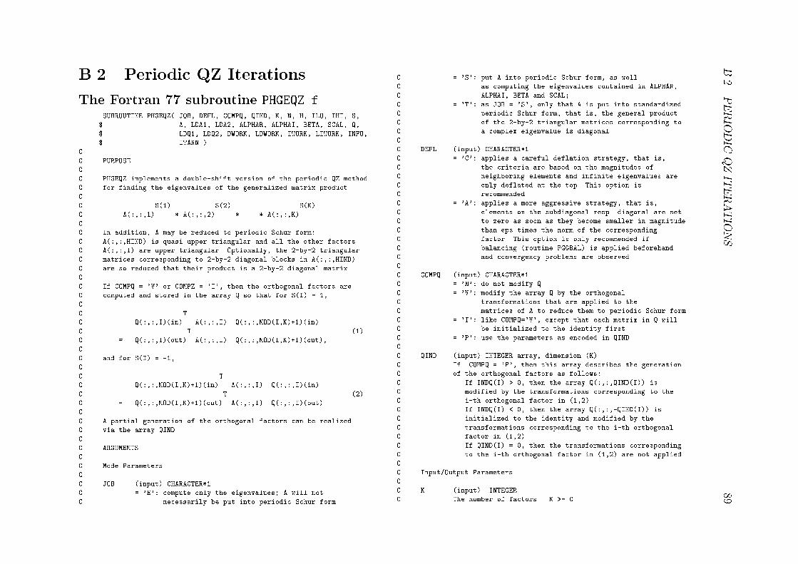
B.2.PERIODICQZITERATIONS89
B.2 Periodic QZ IterationsThe Fortran 77 subroutine PHGEQZ.fSUBROUTINE PHGEQZ( JOB, DEFL, COMPQ, QIND, K, N, H, ILO, IHI, S,$ A, LDA1, LDA2, ALPHAR, ALPHAI, BETA, SCAL, Q,$ LDQ1, LDQ2, DWORK, LDWORK, IWORK, LIWORK, INFO,$ IWARN )CC PURPOSECC PHGEQZ implements a double-shift version of the periodic QZ methodC for finding the eigenvalues of the generalized matrix productCC S(1) S(2) S(K)C A(:,:,1) * A(:,:,2) * ... * A(:,:,K)CC In addition, A may be reduced to periodic Schur form:C A(:,:,HIND) is quasi upper triangular and all the other factorsC A(:,:,I) are upper triangular. Optionally, the 2-by-2 triangularC matrices corresponding to 2-by-2 diagonal blocks in A(:,:,HIND)C are so reduced that their product is a 2-by-2 diagonal matrix.CC If COMPQ = 'V' or COMPZ = 'I', then the orthogonal factors areC computed and stored in the array Q so that for S(I) = 1,CC TC Q(:,:,I)(in) A(:,:,I) Q(:,:,MOD(I,K)+1)(in)C T (1)C = Q(:,:,I)(out) A(:,:,I) Q(:,:,MOD(I,K)+1)(out),CC and for S(I) = -1,CC TC Q(:,:,MOD(I,K)+1)(in) A(:,:,I) Q(:,:,I)(in)C T (2)C = Q(:,:,MOD(I,K)+1)(out) A(:,:,I) Q(:,:,I)(out).CC A partial generation of the orthogonal factors can be realizedC via the array QIND.CC ARGUMEMTSCC Mode ParametersCC JOB (input) CHARACTER*1C = 'E': compute only the eigenvalues; A will notC necessarily be put into periodic Schur form.C = 'S': put A into periodic Schur form, as wellC as computing the eigenvalues contained in ALPHAR,C ALPHAI, BETA and SCAL;C = 'T': as JOB = 'S', only that A is put into standardizedC periodic Schur form, that is, the general productC of the 2-by-2 triangular matrices corresponding toC a complex eigenvalue is diagonal.CC DEFL (input) CHARACTER*1C = 'C': applies a careful deflation strategy, that is,C the criteria are based on the magnitudes ofC neighboring elements and infinite eigenvalues areC only deflated at the top. This option isC recommended.C = 'A': applies a more aggressive strategy, that is,C elements on the subdiagonal resp. diagonal are setC to zero as soon as they become smaller in magnitudeC than eps times the norm of the correspondingC factor. This option is only recommended ifC balancing (routine PGGBAL) is applied beforehandC and convergency problems are observed.CC COMPQ (input) CHARACTER*1C = 'N': do not modify Q.C = 'V': modify the array Q by the orthogonalC transformations that are applied to theC matrices of A to reduce them to periodic Schur form.C = 'I': like COMPQ='V', except that each matrix in Q willC be initialized to the identity first.C = 'P': use the parameters as encoded in QIND.CC QIND (input) INTEGER array, dimension (K).C If COMPQ = 'P', then this array describes the generationC of the orthogonal factors as follows:C If INDQ(I) > 0, then the array Q(:,:,QIND(I)) isC modified by the transformations corresponding to theC i-th orthogonal factor in (1,2).C If INDQ(I) < 0, then the array Q(:,:,-QIND(I)) isC initialized to the identity and modified by theC transformations corresponding to the i-th orthogonalC factor in (1,2).C If QIND(I) = 0, then the transformations correspondingC to the i-th orthogonal factor in (1,2) are not applied.CC Input/Output ParametersCC K (input) INTEGERC The number of factors. K >= 0.
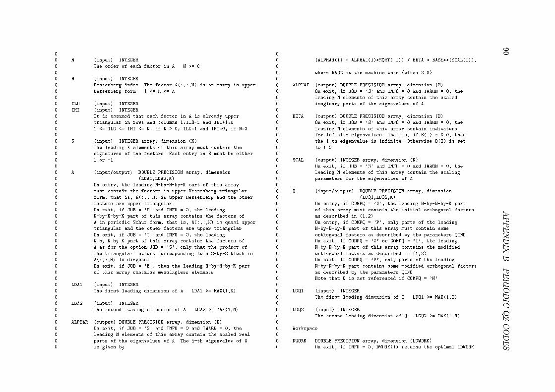
90APPENDIXB.PERIODICQZCODES
CC N (input) INTEGERC The order of each factor in A. N >= 0.CC H (input) INTEGERC Hessenberg index. The factor A(:,:,H) is on entry in upperC Hessenberg form. 1 <= H <= K.CC ILO (input) INTEGERC IHI (input) INTEGERC It is assumed that each factor in A is already upperC triangular in rows and columns 1:ILO-1 and IHI+1:N.C 1 <= ILO <= IHI <= N, if N > 0; ILO=1 and IHI=0, if N=0.CC S (input) INTEGER array, dimension (K)C The leading K elements of this array must contain theC signatures of the factors. Each entry in S must be eitherC 1 or -1.CC A (input/output) DOUBLE PRECISION array, dimensionC (LDA1,LDA2,K)C On entry, the leading N-by-N-by-K part of this arrayC must contain the factors in upper Hessenberg-triangularC form, that is, A(:,:,H) is upper Hessenberg and the otherC factors are upper triangular.C On exit, if JOB = 'S' and INFO = 0, the leadingC N-by-N-by-K part of this array contains the factors ofC A in periodic Schur form, that is, A(:,:,H) is quasi upperC triangular and the other factors are upper triangular.C On exit, if JOB = 'T' and INFO = 0, the leadingC N-by-N-by-K part of this array contains the factors ofC A as for the option JOB = 'S', only that the product ofC the triangular factors corresponding to a 2-by-2 block inC A(:,:,H) is diagonal.C On exit, if JOB = 'E', then the leading N-by-N-by-K partC of this array contains meaningless elements.CC LDA1 (input) INTEGERC The first leading dimension of A. LDA1 >= MAX(1,N).CC LDA2 (input) INTEGERC The second leading dimension of A. LDA2 >= MAX(1,N).CC ALPHAR (output) DOUBLE PRECISION array, dimension (N)C On exit, if JOB = 'S' and INFO = 0 and IWARN = 0, theC leading N elements of this array contain the scaled realC parts of the eigenvalues of A. The i-th eigenvalue of AC is given by
CC (ALPHAR(I) + ALPHAI(I)*SQRT(-1)) / BETA * BASE**(SCAL(I)),CC where BASE is the machine base (often 2.0).CC ALPHAI (output) DOUBLE PRECISION array, dimension (N)C On exit, if JOB = 'S' and INFO = 0 and IWARN = 0, theC leading N elements of this array contain the scaledC imaginary parts of the eigenvalues of A.CC BETA (output) DOUBLE PRECISION array, dimension (N)C On exit, if JOB = 'S' and INFO = 0 and IWARN = 0, theC leading N elements of this array contain indicatorsC for infinite eigenvalues. That is, if B(I) = 0.0, thenC the i-th eigenvalue is infinite. Otherwise B(I) is setC to 1.0.CC SCAL (output) INTEGER array, dimension (N)C On exit, if JOB = 'S' and INFO = 0 and IWARN = 0, theC leading N elements of this array contain the scalingC parameters for the eigenvalues of A.CC Q (input/output) DOUBLE PRECISION array, dimensionC (LDQ1,LDQ2,K)C On entry, if COMPQ = 'V', the leading N-by-N-by-K partC of this array must contain the initial orthogonal factorsC as described in (1,2).C On entry, if COMPQ = 'P', only parts of the leadingC N-by-N-by-K part of this array must contain someC orthogonal factors as described by the parameters QIND.C On exit, if COMPQ = 'V' or COMPQ = 'I', the leadingC N-by-N-by-K part of this array contains the modifiedC orthogonal factors as described in (1,2).C On exit, if COMPQ = 'P', only parts of the leadingC N-by-N-by-K part contains some modified orthogonal factorsC as described by the parameters QIND.C Note that Q is not referenced if COMPQ = 'N'.CC LDQ1 (input) INTEGERC The first leading dimension of Q. LDQ1 >= MAX(1,N).CC LDQ2 (input) INTEGERC The second leading dimension of Q. LDQ2 >= MAX(1,N).CC WorkspaceCC DWORK DOUBLE PRECISION array, dimension (LDWORK)C On exit, if INFO = 0, DWORK(1) returns the optimal LDWORK.

B.2.PERIODICQZITERATIONS91
C On exit, if INFO = -22, DWORK(1) returns the minimumC value of LDWORK.CC LDWORK INTEGERC The length of the array DWORK.C If DEFL = 'C', LDWORK >= MAX( 1,MAX( 2*N,8*K ) );C if DEFL = 'A', LDWORK >= MAX( 1,K + MAX( 2*N,8*K ) ).CC IWORK INTEGER array, dimension (LIWORK)C On exit, if INFO = 0, IWORK(1) returns the optimal LIWORK.C On exit, if INFO = -24, IWORK(1) returns the minimumC value of LIWORK.CC LIWORK INTEGERC The length of the array IWORK. LIWORK >= MAX( 1,2*K ).CC Error IndicatorC
C INFO INTEGERC = 0 : successful exit;C < 0 : if INFO = -i, the i-th argument had an illegalC value;C = 1,..,N : the periodic QZ iteration did not converge.C A is not in periodic Schur form, butC ALPHAR(i), ALPHAI(i), BETA(i) and SCAL(i), forC i = INFO+1,...,N should be correct.CC IWARN INTEGERC = 0 : no warnings;C = 1,..,N-1 : A is in periodic Schur form, but theC algorithm was not able to reveal informationC about the eigenvalues from the 2-by-2C blocks.C ALPHAR(i), ALPHAI(i), BETA(i) and SCAL(i),C can be incorrect for i = 1, ..., IWARN+1.

92 APPENDIX B. PERIODIC QZ CODES

Appendix CBlock Toeplitz Codes
C.1 Linear Systems with s.p.d. BlockToeplitz Matrices(Inverse) Cholesky Factor: MB02CD.fSUBROUTINE MB02CD( JOB, TYPET, K, N, T, LDT, G, LDG, L, LDL, R,$ LDR, DWORK, LDWORK, INFO )CC PURPOSECC To compute the Cholesky factor and the generator and/or theC Cholesky factor of the inverse of a symmetric positive definiteC block Toeplitz matrix T, given the first block row or column ofC T. Transformation information is stored.CC ARGUMENTSCC Mode ParametersCC JOB CHARACTER*1C Specifies the output of the routine as follows:C = 'G': only compute the generator G of the inverse;C = 'R': compute the generator G of the inverse and theC Cholesky factor R of T;C = 'L': compute the generator G and the Cholesky factorC L of the inverse;
C = 'A': compute the generator G, the Cholesky factor LC of the inverse and the Cholesky factor R of T;C = 'O': only compute the Cholesky factor R of T.CC TYPET CHARACTER*1C Specifies the type of T:C = 'R': T contains the first block row of a s.p.d. blockC Toeplitz matrix, if demanded the Cholesky factorsC R and L are upper and lower triangular,C respectively, G contains the transposed generatorC of the inverse;C = 'C': T contains the first block column of a s.p.d.C block Toeplitz matrix, if demanded the CholeskyC factors R and L are lower and upper triangular,C respectively, G contains the generator of theC inverse. This choice results in a column orientedC algorithm which is usually faster.CC Input/Output ParametersCC K (input) INTEGERC The number of rows or columns in T, which should be equalC to the blocksize. K >= 0.CC N (input) INTEGERC The number of blocks in T. N >= 0.CC T (input/output) DOUBLE PRECISION array, dimensionC (LDT,N*K) or (LDT,K)C On entry, the leading K-by-N*K / N*K-by-K part of thisC array contains the first block row / column of aC s.p.d. block Toeplitz matrix.C On exit, if INFO = 0, then the leading K-by-N*K / N*K-by-KC part of this array contains, in the first K-by-K block,C the upper / lower Cholesky factor of T(1:K,1:K), and inC the remaining part, the Householder transformationsC applied during the process.CC LDT INTEGERC The leading dimension of the array T.C LDT >= MAX(1,K), if TYPET = 'R';C LDT >= MAX(1,N*K), if TYPET = 'C'.CC G (output) DOUBLE PRECISION array, dimension (LDG,N*K) orC (LDG,2*K)C If INFO = 0 and JOB = 'G', 'R', 'L', or 'A', then theC leading 2*K-by-N*K / N*K-by-2*K part of this arrayC contains, in the first K-by-K block of the second block
93

94APPENDIXC.BLOCKTOEPLITZCODES
C row / column, the lower right block of L, which isC necessary for the updating SLICOT routine MB02??, andC in the remaining part, the generator of the inverse of T.C To actual obtain a generator one has to setCC G(K+1:2*K, 1:K) = 0, if TYPET = 'R';C G(1:K, K+1:2*K) = 0, if TYPET = 'C'.CC LDG INTEGERC The leading dimension of the array G.C LDG >= MAX(1,2*K), if TYPET = 'R' andC JOB = 'G', 'R', 'L', or 'A';C LDG >= MAX(1,N*K), if TYPET = 'C' andC JOB = 'G', 'R', 'L', or 'A';C LDG >= 1, if JOB = 'O'.CC L (output) DOUBLE PRECISION array, dimension (LDL,N*K)C If INFO = 0 and JOB = 'L', or 'A', then the leadingC N*K-by-N*K part of this array contains the lower / upperC Cholesky factor of the inverse of T.C The elements in the upper / lower triangular part are notC referenced.CC LDL INTEGERC The leading dimension of the array L.C LDL >= MAX(1,N*K), if JOB = 'L', or 'A';C LDL >= 1, if JOB = 'G', 'R', or 'O'.CC R (output) DOUBLE PRECISION array, dimension (LDR,N*K)C If INFO = 0 and JOB = 'R', 'A', or 'O', then the leadingC N*K-by-N*K part of this array contains the upper / lowerC Cholesky factor of T.C The elements in the lower / upper triangular part are notC referenced.CC LDR INTEGERC The leading dimension of the array R.C LDR >= MAX(1,N*K), if JOB = 'R', 'A', or 'O';C LDR >= 1, if JOB = 'G', or 'L'.CC WorkspaceCC DWORK DOUBLE PRECISION array, dimension (LDWORK)C On exit, if INFO = 0, DWORK(1) returns the optimalC value of LDWORK, and the elements 2 : 3*(N-1)*K+1 of DWORKC contain information about the hyperbolic rotations andC Householder transformations applied during the process.C On exit, if INFO = -14, DWORK(1) returns the minimumC value of LDWORK.CC LDWORK INTEGERC The length of the array DWORK. LDWORK >= MAX(1,3*N*K).CC Error IndicatorCC INFO INTEGERC = 0: successful exit;C < 0: if INFO = -i, the i-th argument had an illegalC value;C = 1: the reduction algorithm failed. The block ToeplitzC matrix associated with T is not (numerically)C positive definite.Updating the (Inverse) Cholesky Factor:MB02CD.fSUBROUTINE MB02DD( JOB, TYPET, K, M, N, TA, LDTA, T, LDT, G,$ LDG, L, LDL, R, LDR, DWORK, LDWORK, INFO )CC PURPOSECC To update the Cholesky factor and the generator and/or theC Cholesky factor of the inverse of a symmetric positive definiteC (s.p.d.) block Toeplitz matrix T, given the information fromC a previous factorization and additional blocks of its firstC block row, or its first block column, depending on the routineC parameter TYPET. Transformation information is stored.CC ARGUMENTSCC Mode ParametersCC JOB CHARACTER*1C Specifies the output of the routine, as follows:C = 'R': updates the generator G of the inverse andC computes the new columns / rows for the CholeskyC factor R of T;C = 'A': updates the generator G, computes the newC columns / rows for the Cholesky factor R of T andC the new rows / columns for the Cholesky factor LC of the inverse;C = 'O': only computes the new columns / rows for theC Cholesky factor R of T.CC TYPET CHARACTER*1

C.1.LINEARSYSTEMSWITHS.P.D.BLOCKTOEPLITZMATRICES95
C Specifies the type of T, as follows:C = 'R': the first block row of an s.p.d. block ToeplitzC matrix was/is defined; if demanded, the CholeskyC factors R and L are upper and lower triangular,C respectively, and G contains the transposedC generator of the inverse;C = 'C': the first block column of an s.p.d. block ToeplitzC matrix was/is defined; if demanded, the CholeskyC factors R and L are lower and upper triangular,C respectively, and G contains the generator of theC inverse. This choice results in a column orientedC algorithm which is usually faster.C Note: in this routine, the notation x / y means thatC x corresponds to TYPET = 'R' and y corresponds toC TYPET = 'C'.CC Input/Output ParametersCC K (input) INTEGERC The number of rows / columns in T, which should be equalC to the blocksize. K >= 0.CC M (input) INTEGERC The number of blocks in TA. M >= 0.CC N (input) INTEGERC The number of blocks in T. N >= 0.CC TA (input/output) DOUBLE PRECISION array, dimensionC (LDTA,M*K) / (LDTA,K)C On entry, the leading K-by-M*K / M*K-by-K part of thisC array must contain the (N+1)-th to M-th blocks in theC first block row / column of an s.p.d. block ToeplitzC matrix.C On exit, if INFO = 0, the leading K-by-M*K / M*K-by-K partC of this array contains information on the HouseholderC transformations used, such that the arrayCC [ T TA ] / [ T ]C [ TA ]CC serves as the new transformation matrix T for furtherC applications of this routine.CC LDTA INTEGERC The leading dimension of the array TA.C LDTA >= MAX(1,K), if TYPET = 'R';C LDTA >= MAX(1,M*K), if TYPET = 'C'.CC T (input) DOUBLE PRECISION array, dimension (LDT,N*K) /C (LDT,K)C The leading K-by-N*K / N*K-by-K part of this array mustC contain transformation information generated by the SLICOTC Library routine MB02CD, i.e., in the first K-by-K block,C the upper / lower Cholesky factor of T(1:K,1:K), and inC the remaining part, the Householder transformationsC applied during the initial factorization process.CC LDT INTEGERC The leading dimension of the array T.C LDT >= MAX(1,K), if TYPET = 'R';C LDT >= MAX(1,N*K), if TYPET = 'C'.CC G (input/output) DOUBLE PRECISION array, dimensionC (LDG,( N + M )*K) / (LDG,2*K)C On entry, if JOB = 'R', or 'A', then the leadingC 2*K-by-N*K / N*K-by-2*K part of this array must contain,C in the first K-by-K block of the second block row /C column, the lower right block of the Cholesky factor ofC the inverse of T, and in the remaining part, the generatorC of the inverse of T.C On exit, if INFO = 0 and JOB = 'R', or 'A', then theC leading 2*K-by-( N + M )*K / ( N + M )*K-by-2*K part ofC this array contains the same information as on entry, nowC for the updated Toeplitz matrix. Actually, to obtain aC generator of the inverse one has to setC G(K+1:2*K, 1:K) = 0, if TYPET = 'R';C G(1:K, K+1:2*K) = 0, if TYPET = 'C'.CC LDG INTEGERC The leading dimension of the array G.C LDG >= MAX(1,2*K), if TYPET = 'R' and JOB = 'G', or 'A';C LDG >= MAX(1,( N + M )*K),C if TYPET = 'R' and JOB = 'G', or 'A';C LDG >= 1, if JOB = 'O'.CC L (output) DOUBLE PRECISION array, dimensionC (LDL,( N + M )*K) / (LDL,M*K)C If INFO = 0 and JOB = 'A', then the leadingC M*K-by-( N + M )*K / ( N + M )*K-by-M*K part of thisC array contains the last M*K columns / rows of the lower /C upper Cholesky factor of the inverse of T. The elementsC in the strictly upper / lower triangular part are notC referenced.CC LDL INTEGER
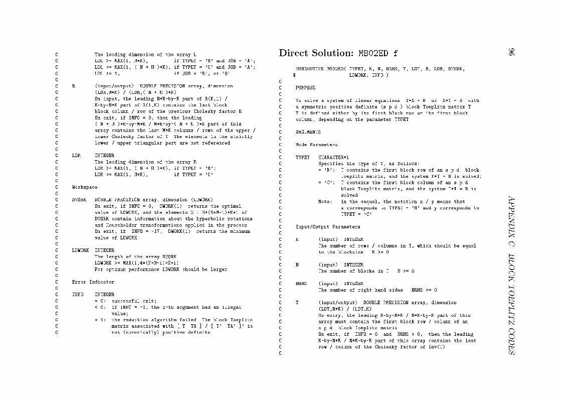
96APPENDIXC.BLOCKTOEPLITZCODES
C The leading dimension of the array L.C LDL >= MAX(1, M*K), if TYPET = 'R' and JOB = 'A';C LDL >= MAX(1, ( N + M )*K), if TYPET = 'C' and JOB = 'A';C LDL >= 1, if JOB = 'R', or 'O'.CC R (input/output) DOUBLE PRECISION array, dimensionC (LDR,M*K) / (LDR,( N + M )*K)C On input, the leading N*K-by-K part of R(K,1) /C K-by-N*K part of R(1,K) contains the last blockC block column / row of the previous Cholesky factor R.C On exit, if INFO = 0, then the leadingC ( N + M )*K-by-M*K / M*K-by-( N + M )*K part of thisC array contains the last M*K columns / rows of the upper /C lower Cholesky factor of T. The elements in the strictlyC lower / upper triangular part are not referenced.CC LDR INTEGERC The leading dimension of the array R.C LDR >= MAX(1, ( N + M )*K), if TYPET = 'R';C LDR >= MAX(1, M*K), if TYPET = 'C'.CC WorkspaceCC DWORK DOUBLE PRECISION array, dimension (LDWORK)C On exit, if INFO = 0, DWORK(1) returns the optimalC value of LDWORK, and the elements 2 : 3*(N+M-1)*K+1 ofC DWORK contain information about the hyperbolic rotationsC and Householder transformations applied in the process.C On exit, if INFO = -17, DWORK(1) returns the minimumC value of LDWORK.CC LDWORK INTEGERC The length of the array DWORK.C LDWORK >= MAX(1,4*(N+M-1)*K+1).C For optimum performance LDWORK should be larger.CC Error IndicatorCC INFO INTEGERC = 0: successful exit;C < 0: if INFO = -i, the i-th argument had an illegalC value;C = 1: the reduction algorithm failed. The block ToeplitzC matrix associated with [ T TA ] / [ T' TA' ]' isC not (numerically) positive definite.Direct Solution: MB02ED.fSUBROUTINE MB02ED( TYPET, K, N, NRHS, T, LDT, B, LDB, DWORK,$ LDWORK, INFO )CC PURPOSECC To solve a system of linear equations T*X = B or X*T = B withC a symmetric positive definite (s.p.d.) block Toeplitz matrix T.C T is defined either by its first block row or its first blockC column, depending on the parameter TYPET.CC ARGUMENTSCC Mode ParametersCC TYPET CHARACTER*1C Specifies the type of T, as follows:C = 'R': T contains the first block row of an s.p.d. blockC Toeplitz matrix, and the system X*T = B is solved;C = 'C': T contains the first block column of an s.p.d.C block Toeplitz matrix, and the system T*X = B isC solved.C Note: in the sequel, the notation x / y means thatC x corresponds to TYPET = 'R' and y corresponds toC TYPET = 'C'.CC Input/Output ParametersCC K (input) INTEGERC The number of rows / columns in T, which should be equalC to the blocksize. K >= 0.CC N (input) INTEGERC The number of blocks in T. N >= 0.CC NRHS (input) INTEGERC The number of right hand sides. NRHS >= 0.CC T (input/output) DOUBLE PRECISION array, dimensionC (LDT,N*K) / (LDT,K)C On entry, the leading K-by-N*K / N*K-by-K part of thisC array must contain the first block row / column of anC s.p.d. block Toeplitz matrix.C On exit, if INFO = 0 and NRHS > 0, then the leadingC K-by-N*K / N*K-by-K part of this array contains the lastC row / column of the Cholesky factor of inv(T).C

C.1.LINEARSYSTEMSWITHS.P.D.BLOCKTOEPLITZMATRICES97
C LDT INTEGERC The leading dimension of the array T.C LDT >= MAX(1,K), if TYPET = 'R';C LDT >= MAX(1,N*K), if TYPET = 'C'.CC B (input/output) DOUBLE PRECISION array, dimensionC (LDB,N*K) / (LDB,NRHS)C On entry, the leading NRHS-by-N*K / N*K-by-NRHS part ofC this array must contain the right hand side matrix B.C On exit, the leading NRHS-by-N*K / N*K-by-NRHS part ofC this array contains the solution matrix X.CC LDB INTEGERC The leading dimension of the array B.C LDB >= MAX(1,NRHS), if TYPET = 'R';C LDB >= MAX(1,N*K), if TYPET = 'C'.CC WorkspaceCC DWORK DOUBLE PRECISION array, dimension (LDWORK)C On exit, if INFO = 0, DWORK(1) returns the optimalC value of LDWORK.C On exit, if INFO = -10, DWORK(1) returns the minimumC value of LDWORK.CC LDWORK INTEGERC The length of the array DWORK. LDWORK >= N*K*K+(N+2)*K+1.C For optimum performance LDWORK should be larger.CC Error IndicatorCC INFO INTEGERC = 0: successful exit;C < 0: if INFO = -i, the i-th argument had an illegalC value;C = 1: the reduction algorithm failed. The Toeplitz matrixC associated with T is not (numerically) positiveC definite.Incomplete Cholesky Factorization: MB02FD.fSUBROUTINE MB02FD( TYPET, K, N, P, S, T, LDT, R, LDR, DWORK,$ LDWORK, INFO )CC PURPOSECC To compute the incomplete Cholesky (ICC) factor of a symmetricC positive definite (s.p.d.) block Toeplitz matrix T, defined byC either its first block row, or its first block column, dependingC on the routine parameter TYPET.CC By subsequent calls of this routine, further rows / columns ofC the Cholesky factor can be added.C Furthermore, the generator of the Schur complement of the leadingC (P+S)*K-by-(P+S)*K block in T is available, which can be used,C e.g., for measuring the quality of the ICC factorization.CC ARGUMENTSCC Mode ParametersCC TYPET CHARACTER*1C Specifies the type of T, as follows:C = 'R': T contains the first block row of an s.p.d. blockC Toeplitz matrix; the ICC factor R is upperC trapezoidal;C = 'C': T contains the first block column of an s.p.d.C block Toeplitz matrix; the ICC factor R is lowerC trapezoidal; this choice leads to betterC localized memory references and hence a fasterC algorithm.C Note: in the sequel, the notation x / y means thatC x corresponds to TYPET = 'R' and y corresponds toC TYPET = 'C'.CC Input/Output ParametersCC K (input) INTEGERC The number of rows / columns in T, which should be equalC to the blocksize. K >= 0.CC N (input) INTEGERC The number of blocks in T. N >= 0.CC P (input) INTEGERC The number of previously computed block rows / columnsC of R. 0 <= P <= N.CC S (input) INTEGERC The number of block rows / columns of R to compute.C 0 <= S <= N-P.CC T (input/output) DOUBLE PRECISION array, dimensionC (LDT,(N-P)*K) / (LDT,K)C On entry, if P = 0, then the leading K-by-N*K / N*K-by-K

98APPENDIXC.BLOCKTOEPLITZCODES
C part of this array must contain the first block row /C column of an s.p.d. block Toeplitz matrix.C If P > 0, the leading K-by-(N-P)*K / (N-P)*K-by-K mustC contain the negative generator of the Schur complement ofC the leading P*K-by-P*K part in T, computed from previousC calls of this routine.C On exit, if INFO = 0, then the leading K-by-(N-P)*K /C (N-P)*K-by-K part of this array contains, in the firstC K-by-K block, the upper / lower Cholesky factor ofC T(1:K,1:K), in the following S-1 K-by-K blocks, theC Householder transformations applied during the process,C and in the remaining part, the negative generator of theC Schur complement of the leading (P+S)*K-by(P+S)*K partC in T.CC LDT INTEGERC The leading dimension of the array T.C LDT >= MAX(1,K), if TYPET = 'R';C LDT >= MAX(1,(N-P)*K), if TYPET = 'C'.CC R (input/output) DOUBLE PRECISION array, dimensionC (LDR, N*K) / (LDR, S*K ) if P = 0;C (LDR, (N-P+1)*K) / (LDR, (S+1)*K ) if P > 0.C On entry, if P > 0, then the leading K-by-(N-P+1)*K /C (N-P+1)*K-by-K part of this array must contain theC nonzero blocks of the last block row / column in theC ICC factor from a previous call of this routine. Note thatC this part is identical with the positive generator ofC the Schur complement of the leading P*K-by-P*K part in T.C If P = 0, then R is only an output parameter.C On exit, if INFO = 0 and P = 0, then the leadingC S*K-by-N*K / N*K-by-S*K part of this array contains theC upper / lower trapezoidal ICC factor.C On exit, if INFO = 0 and P > 0, then the leadingC (S+1)*K-by-(N-P+1)*K / (N-P+1)*K-by-(S+1)*K part of thisC array contains the upper / lower trapezoidal part of theC P-th to (P+S)-th block rows / columns of the ICC factor.C The elements in the strictly lower / upper trapezoidalC part are not referenced.CC LDR INTEGERC The leading dimension of the array R.C LDR >= MAX(1, S*K ), if TYPET = 'R' and P = 0;C LDR >= MAX(1, (S+1)*K ), if TYPET = 'R' and P > 0;C LDR >= MAX(1, N*K ), if TYPET = 'C' and P = 0;C LDR >= MAX(1, (N-P+1)*K ), if TYPET = 'C' and P > 0;CC Workspace
CC DWORK DOUBLE PRECISION array, dimension (LDWORK)C On exit, if INFO = 0, DWORK(1) returns the optimalC value of LDWORK.C On exit, if INFO = -11, DWORK(1) returns the minimumC value of LDWORK.CC LDWORK INTEGERC The length of the array DWORK.C LDWORK >= MAX(1,(N+1)*K), if P = 0;C LDWORK >= MAX(1,(N-P+2)*K), if P > 0.C For optimum performance LDWORK should be larger.CC Error IndicatorCC INFO INTEGERC = 0: successful exit;C < 0: if INFO = -i, the i-th argument had an illegalC value;C = 1: the reduction algorithm failed; the Toeplitz matrixC associated with T is not (numerically) positiveC definite in its leading (P+S)*K-by-(P+S)*K part.Banded Cholesky Factorization: TPCHB.fSUBROUTINE TPCHB( TYPET, TRIU, K, N, NL, P, S, T, LDT, RB, LDRB,$ DWORK, LDWORK, INFO )CC PURPOSECC To compute the Cholesky factor of a banded symmetric positiveC definite (s.p.d.) block Toeplitz matrix, defined by either itsC first block row, or its first block column, depending on theC routine parameter TYPET.CC By subsequent calls of this routine the Cholesky factor can beC computed block column by block column.CC ARGUMENTSCC Mode ParametersCC TYPET CHARACTER*1CC Specifies the type of T, as follows:C = 'R': T contains the first block row of an s.p.d. blockC Toeplitz matrix; the Cholesky factor is upperC triangular,

C.1.LINEARSYSTEMSWITHS.P.D.BLOCKTOEPLITZMATRICES99
C = 'C': T contains the first block column of an s.p.d.C block Toeplitz matrix; the Cholesky factor isC lower triangular. This choice results in a columnC oriented algorithm which is usually faster.C Note: in the sequel, the notation x / y means thatC x corresponds to TYPET = 'R' and y corresponds toC TYPET = 'C'.CC TRIU CHARACTER*1C The last block in TC = 'N': has no special structure;C = 'T': is lower / upper triangular.CC Input/Output ParametersCC K (input) INTEGERC The number of rows / columns in T, which should be equalC to the blocksize. K >= 0.CC N (input) INTEGERC The number of blocks in T. N >= 1.C If TRIU = 'N', N >= 1;C if TRIU = 'T', N >= 2.CC NL (input) INTEGERC The lower block bandwidth, i.e., NL + 1 is the number ofC nonzero blocks in the first block column of the blockC block Toeplitz matrix.C If TRIU = 'N', 0 <= NL < N;C if TRIU = 'T', 1 <= NL < N.CC P (input) INTEGERC The number of previously computed block rows / columns ofC the Cholesky factor. P <= N.CC S (input) INTEGERC The number of block rows / columns of the Cholesky factorC to compute. 0 <= S <= N - P.CC T (input/output) DOUBLE PRECISION array, dimensionC (LDT,(NL+1)*K) / (LDT,K)C On entry, if P = 0, the leading K-by-(NL+1)*K /C (NL+1)*K-by-K part of this array must contain the firstC block row / column of an s.p.d. block Toeplitz matrix.C On entry, if P > 0, the leading K-by-(NL+1)*K /C (NL+1)*K-by-K part of this array must contain the P-thC block row / column of the Cholesky factor.C On exit, if INFO = 0, then the leading K-by-(NL+1)*K /C (NL+1)*K-by-K part of this array contains the (P+S)-thC block row / column of the Cholesky factor.CC LDT INTEGERC The leading dimension of the array T.C LDT >= MAX(1,K) / MAX(1,(NL+1)*K).CC RB (output) DOUBLE PRECISION array, dimensionC (LDRB,MIN(P+NL+S,N)*K) / (LDRB,MIN(P+S,N)*K)C On entry, if TYPET = 'R' and TRIU = 'N' and P > 0,C the leading (NL+1)*K-by-MIN(NL,N-P)*K part of this arrayC must contain the (P*K+1)-st to ((P+NL)*K)-th columns ofC of the upper Cholesky factor in banded format from aC previous call of this routine.C On entry, if TYPET = 'R' and TRIU = 'T' and P > 0,C the leading (NL*K+1)-by-MIN(NL,N-P)*K part of this arrayC must contain the (P*K+1)-st to (MIN(P+NL,N)*K)-th columnC of the upper Cholesky factor in banded format from aC previous call of this routine.C On exit, if TYPET = 'R' and TRIU = 'N', the leadingC (NL+1)*K-by-MIN(NL+S,N-P)*K part of this array containsC the (P*K+1)-st to (MIN(P+NL+S,N)*K)-th column of the upperC Cholesky factor in banded format.C On exit, if TYPET = 'R' and TRIU = 'T', the leadingC (NL*K+1)-by-MIN(NL+S,N-P)*K part of this array containsC the (P*K+1)-st to (MIN(P+NL+S,N)*K)-th column of the upperC Cholesky factor in banded format.C On exit, if TYPET = 'C' and TRIU = 'N', the leadingC (NL+1)*K-by-MIN(S,N-P)*K part of this array containsC the (P*K+1)-st to (MIN(P+S,N)*K)-th column of the lowerC Cholesky factor in banded format.C On exit, if TYPET = 'C' and TRIU = 'T', the leadingC (NL*K+1)*K-by-MIN(S,N-P)*K part of this array containsC the (P*K+1)-st to (MIN(P+S,N)*K)-th column of the lowerC Cholesky factor in banded format.C For further details regarding the band storage scheme seeC the documentation of the LAPACK routine DPBTF2.CC LDRB INTEGERC The leading dimension of the array RB.C If TRIU = 'N', LDRB >= MAX( (NL+1)*K,1 );C if TRIU = 'T', LDRB >= NL*K+1.CC WorkspaceCC DWORK DOUBLE PRECISION array, dimension (LDWORK)C On exit, if INFO = 0, DWORK(1) returns the optimalC value of LDWORK.
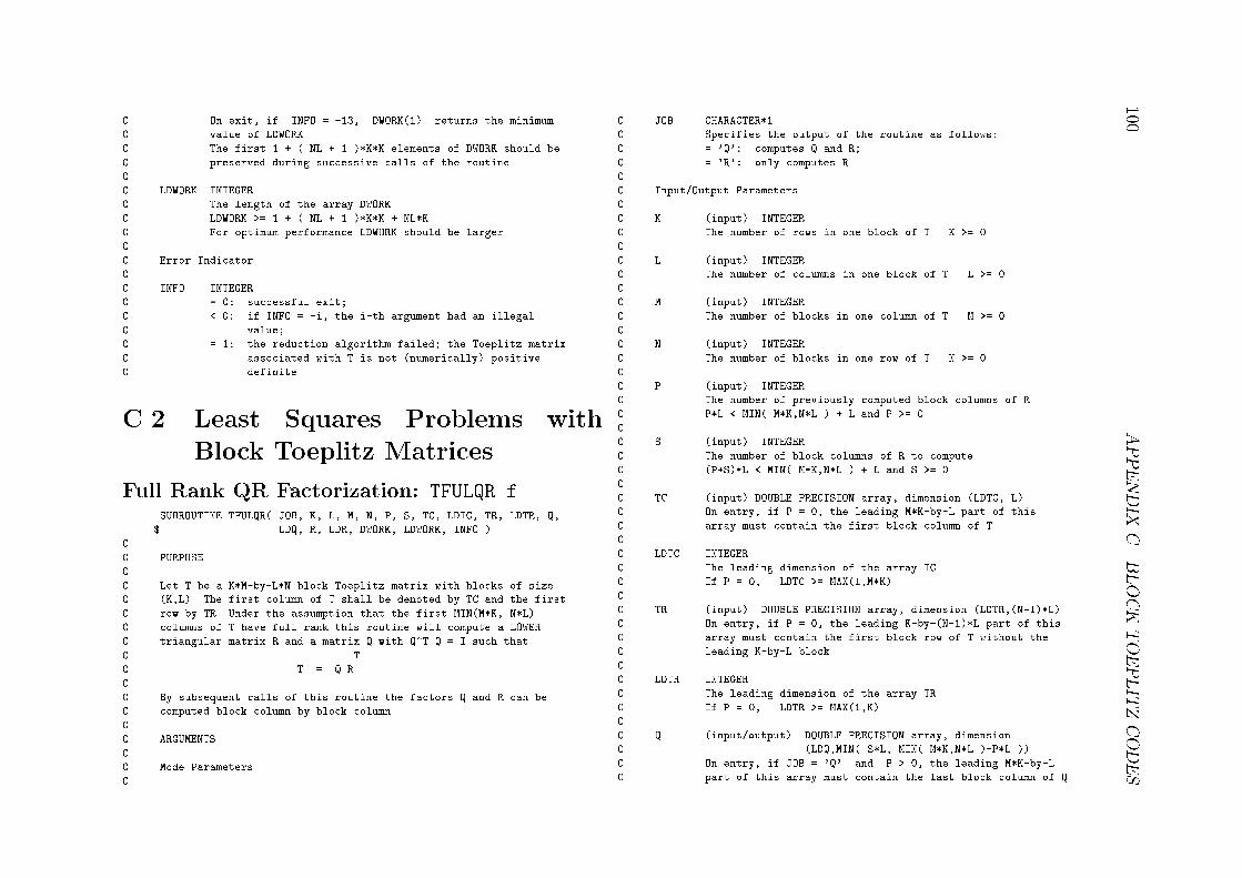
100APPENDIXC.BLOCKTOEPLITZCODES
C On exit, if INFO = -13, DWORK(1) returns the minimumC value of LDWORK.C The first 1 + ( NL + 1 )*K*K elements of DWORK should beC preserved during successive calls of the routine.CC LDWORK INTEGERC The length of the array DWORK.C LDWORK >= 1 + ( NL + 1 )*K*K + NL*KC For optimum performance LDWORK should be larger.CC Error IndicatorCC INFO INTEGERC = 0: successful exit;C < 0: if INFO = -i, the i-th argument had an illegalC value;C = 1: the reduction algorithm failed; the Toeplitz matrixC associated with T is not (numerically) positiveC definite.C.2 Least Squares Problems withBlock Toeplitz MatricesFull Rank QR Factorization: TFULQR.fSUBROUTINE TFULQR( JOB, K, L, M, N, P, S, TC, LDTC, TR, LDTR, Q,$ LDQ, R, LDR, DWORK, LDWORK, INFO )CC PURPOSECC Let T be a K*M-by-L*N block Toeplitz matrix with blocks of sizeC (K,L). The first column of T shall be denoted by TC and the firstC row by TR. Under the assumption that the first MIN(M*K, N*L)C columns of T have full rank this routine will compute a LOWERC triangular matrix R and a matrix Q with Q^T Q = I such thatC TC T = Q R .CC By subsequent calls of this routine the factors Q and R can beC computed block column by block column.CC ARGUMENTSCC Mode ParametersC
C JOB CHARACTER*1C Specifies the output of the routine as follows:C = 'Q': computes Q and R;C = 'R': only computes R.CC Input/Output ParametersCC K (input) INTEGERC The number of rows in one block of T. K >= 0.CC L (input) INTEGERC The number of columns in one block of T. L >= 0.CC M (input) INTEGERC The number of blocks in one column of T. M >= 0.CC N (input) INTEGERC The number of blocks in one row of T. N >= 0.CC P (input) INTEGERC The number of previously computed block columns of R.C P*L < MIN( M*K,N*L ) + L and P >= 0.CC S (input) INTEGERC The number of block columns of R to compute.C (P+S)*L < MIN( M*K,N*L ) + L and S >= 0.CC TC (input) DOUBLE PRECISION array, dimension (LDTC, L)C On entry, if P = 0, the leading M*K-by-L part of thisC array must contain the first block column of T.CC LDTC INTEGERC The leading dimension of the array TC.C If P = 0, LDTC >= MAX(1,M*K).CC TR (input) DOUBLE PRECISION array, dimension (LDTR,(N-1)*L)C On entry, if P = 0, the leading K-by-(N-1)*L part of thisC array must contain the first block row of T without theC leading K-by-L block.CC LDTR INTEGERC The leading dimension of the array TR.C If P = 0, LDTR >= MAX(1,K).CC Q (input/output) DOUBLE PRECISION array, dimensionC (LDQ,MIN( S*L, MIN( M*K,N*L )-P*L ))C On entry, if JOB = 'Q' and P > 0, the leading M*K-by-LC part of this array must contain the last block column of Q

C.2.LEASTSQUARESPROBLEMSWITHBLOCKTOEPLITZMATRICES101
C from a previous call of this routine.C On exit, if JOB = 'Q' and INFO = 0, the leadingC M*K-by-MIN( S*L, MIN( M*K,N*L )-P*L ) part of this arrayC contains the P-th to (P+S)-th block column of the factorC Q.CC LDQ INTEGERC The leading dimension of the array Q.C If JOB = 'Q', LDQ >= MAX(1,M*K).C If JOB = 'R', LDQ >= 1.CC R (input/output) DOUBLE PRECISION array, dimensionC (LDR,MIN( S*L, MIN( M*K,N*L )-P*L ))C On entry, if P > 0, the leading (N-P+1)*L-by-LC part of this array must contain the nozero part of theC last block column of R from a previous call of thisC routine.C One exit, if INFO = 0, the leadingC MAX( N*L,(N-P+1)*L )-by-MIN( S*L, MIN( M*K,N*L )-P*L )C part of this array contains the nonzero parts of the P-thC to (P+S)-th block column of the lower triangular factor R.C Note that elements in the strictly upper triangular partC will not be referenced.CC LDR INTEGERC The leading dimension of the array R.C LDR >= MAX( N*L,(N-P+1)*L )CC WorkspaceCC DWORK DOUBLE PRECISION array, dimension (LDWORK)C Working space.C On exit, if INFO = 0, DWORK(1) returns the optimal valueC of LDWORK.C On exit, if INFO = -17, DWORK(1) returns the minimumC value of LDWORK.C If JOB = 'Q', the first 1 + ( (N-1)*L + M*K )*( 2*K + L )C elements of DWORK should be preserved during successiveC calls of the routine.C If JOB = 'R', the first 1 + (N-1)*L*( 2*K + L ) elementsC of DWORK should be preserved during successive calls ofC the routine.CC LDWORK INTEGERC The length of the array DWORK.C JOB = 'Q':C LDWORK >= 1 + ( M*K + ( N - 1 )*L )*( L + 2*K ) + 6*LC + MAX( M*K,( N - MAX( 1,P )*L ) );C JOB = 'R':C If P = 0,C LDWORK >= MAX( 1 + ( N - 1 )*L*( L + 2*K ) + 6*LC + (N-1)*L, M*K*( L + 1 ) + L );C If P > 0,C LDWORK >= 1 + (N-1)*L*( L + 2*K ) + 6*L + (N-P)*L.C For optimum performance LDWORK should be larger.CC Error IndicatorCC INFO INTEGERC = 0: successful exit;C = 1: the full rank condition for the first MIN(M*K, N*L)C columns of T is (numerically) violated;C < 0: if INFO = -i, the i-th argument had an illegalC value.Low Rank QR Factorization: TDEFQR.fSUBROUTINE TDEFQR( JOB, K, L, M, N, RNK, TOL1, TOL2, TC, LDTC,$ TR, LDTR, Q, LDQ, R, LDR, JPVT, DWORK, LDWORK,$ INFO )CC PURPOSECC Let T be a K*M-by-L*N block Toeplitz matrix with blocks of sizeC (K,L). This routine computes a low rank QR factorization withC column pivotingC TC T P = Q R ,CC where R is lower trapezoidal and Q^T Q = I. The number of columnsC in R is equivalent to the numerical rank of T w.r.t. the givenC tolerance TOL1.C Note that the pivoting scheme is local, i.e., only columnsC belonging to the same block in T are permuted.CC ARGUMENTSCC Mode ParametersCC JOB CHARACTER*1C Specifies the output of the routine as follows:C = 'Q': computes Q and R;C = 'R': only computes R.CC Input/Output ParametersC

102APPENDIXC.BLOCKTOEPLITZCODES
C K (input) INTEGERC The number of rows in one block of T. K >= 0.CC L (input) INTEGERC The number of columns in one block of T. L >= 0.CC M (input) INTEGERC The number of blocks in one column of T. M >= 0.CC N (input) INTEGERC The number of blocks in one row of T. N >= 0.CC RNK (output) INTEGERC The number of columns in R which is equivalent to theC numerical rank of T.CC TOL1 (input/output) DOUBLE PRECISIONC On entry, if TOL1 >= 0.0, the user supplied diagonalC tolerance.C On exit, if TOL1 < 0.0, the default diagonal tolerance.CC TOL2 (input/output) DOUBLE PRECISIONC On entry, if TOL2 >= 0.0, the user supplied offdiagonalC tolerance.C On exit, if TOL2 < 0.0, the default offdiagonal tolerance.CC TC (input) DOUBLE PRECISION array, dimension (LDTC, L)C The leading M*K-by-L part of this array must containC the first block column of T.CC LDTC INTEGERC The leading dimension of the array TC.C LDTC >= MAX(1,M*K).CC TR (input) DOUBLE PRECISION array, dimension (LDTR,(N-1)*L)C The leading K-by-(N-1)*L part of this array must containC the first block row of T without the leading K-by-LC block.CC LDTR INTEGERC The leading dimension of the array TR. LDTR >= MAX(1,K).CC Q (output) DOUBLE PRECISION array, dimension (LDQ,RNK)C If JOB = 'Q', then the leading M*K-by-RNK part of thisC array contains the factor Q.CC LDQ INTEGERC The leading dimension of the array Q.C If JOB = 'Q', LDQ >= MAX(1,M*K).C If JOB = 'R', LDQ >= 1.CC R (output) DOUBLE PRECISION array, dimension (LDQ,RNK)C The leading N*L-by-RNK part of this array contains theC lower trapezoidal factor R.CC LDR INTEGERC The leading dimension of the array R.C LDR >= MAX(1,N*L)CC JPVT (output) INTEGER array, dimension (MIN(M*K,N*L))C On exit, if JPVT(j) = k, then the j-th column of T*P wasC the k-th column of T.CC WorkspaceCC DWORK DOUBLE PRECISION array, dimension (LDWORK)C Working space.C On exit, if INFO = 0, DWORK(1) returns the optimal valueC of LDWORK.C On exit, if INFO = -19, DWORK(1) returns the minimumC value of LDWORK.CC LDWORK INTEGERC The length of the array DWORK.C JOB = 'Q':C LDWORK >= MAX( 1,( M*K + ( N - 1 )*L )*( L + 2*K ) + 5*LC + MAX(M*K,(N-1)*L) )C JOB = 'R':C LDWORK >= MAX( 1, MAX (C ( N - 1 )*L*( L + 2*K + 1 ) + 5*L,C M*K*( L + 1 ) + L ) )CC Error IndicatorCC INFO INTEGERC = 0: successful exit;C = 1: the algorithm did not succeed in removing linearlyC dependent columns of T;C < 0: if INFO = -i, the i-th argument had an illegalC value.Banded QR Factorization: TPQRB.fSUBROUTINE TPQRB( TRIU, K, L, M, ML, N, NU, P, S, TR, LDTR, TC,$ LDTC, RB, LDRB, DWORK, LDWORK, INFO )C
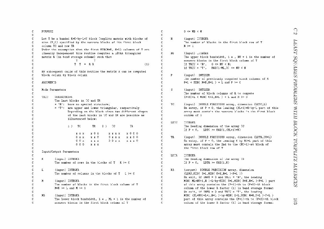
C.2.LEASTSQUARESPROBLEMSWITHBLOCKTOEPLITZMATRICES103
C PURPOSECC Let T be a banded K*M-by-L*N block Toeplitz matrix with blocks ofC size (K,L) specified by the nonzero blocks of its first blockC column TC and row TR.C Under the assumption that the first MIN(M*K, N*L) columns of T areC linearly independent this routine computes a LOWER triangularC matrix R (in band storage scheme) such thatC T TC T T = R R . (1)CC By subsequent calls of this routine the matrix R can be computedC block column by block column.CC ARGUMENTSCC Mode ParametersCC TRIU CHARACTER*1C The last blocks in TC and TRC = 'N': have no special structure;C = 'T': are upper and lower triangular, respectively.C Depending on the block sizes two different shapesC of the last blocks in TC and TR are possible asC illustrated below:CC 1.) TC TR 2.) TC TRCC x x x x 0 0 x x x x x 0 0 0C 0 x x x x 0 0 x x x x x 0 0C 0 0 x x x x 0 0 x x x x x 0C 0 0 0 x x xCC Input/Output ParametersCC K (input) INTEGERC The number of rows in the blocks of T. K >= 0.CC L (input) INTEGERC The number of columns in the blocks of T. L >= 0.CC M (input) INTEGERC The number of blocks in the first block column of T.C M*K >= L and M >= 1.CC MB (input) INTEGERC The lower block bandwidth, i.e., ML + 1 is the number ofC nonzero blocks in the first block column of T.C 0 <= MB < M.CC N (input) INTEGERC The number of blocks in the first block row of T.C N >= 1.CC NU (input) INTEGERC The upper block bandwidth, i.e., NU + 1 is the number ofC nonzero blocks in the first block column of T.C If TRIU = 'N', 0 <= NU < N;C if TRIU = 'T', MAX(1-ML,0) <= NU < N.CC P (input) INTEGERC The number of previously computed block columns of R.C P*L < MIN( M*K,N*L ) + L and P >= 0.CC S (input) INTEGERC The number of block columns of R to compute.C (P+S)*L < MIN( M*K,N*L ) + L and S >= 0.CC TC (input) DOUBLE PRECISION array, dimension (LDTC,L)C On entry, if P = 0, the leading (ML+1)*K-by-L part of thisC array must contain the nonzero blocks in the first blockC column of T.CC LDTC INTEGERC The leading dimension of the array TC.C If P = 0, LDTC >= MAX(1,(ML+1)*K).CC TR (input) DOUBLE PRECISION array, dimension (LDTR,NU*L)C On entry, if P = 0, the leading K-by-NU*L part of thisC array must contain the 2nd to the (NU+1)-st block ofC the first block row of T.CC LDTR INTEGERC The leading dimension of the array TR.C If P = 0, LDTR >= MAX(1,K).CC RB (output) DOUBLE PRECISION array, dimensionC (LDRB,MIN( S*L,MIN( M*K,N*L )-P*L ))C On exit, if INFO = 0 and TRIU = 'N', the leadingC MIN( ML+NU+1,N )*L-by-MIN( S*L,MIN( M*K,N*L )-P*L ) partC of this array contains the (P+1)-th to (P+S)-th blockC column of the lower R factor (1) in band storage format.C On exit, if INFO = 0 and TRIU = 'T', the leadingC MIN( (ML+NU)*L+1,N*L )-by-MIN( S*L,MIN( M*K,N*L )-P*L )C part of this array contains the (P+1)-th to (P+S)-th blockC column of the lower R factor (1) in band storage format.

104APPENDIXC.BLOCKTOEPLITZCODES
C For further details regarding the band storage scheme seeC the documentation of the LAPACK routine DPBTF2.CC LDRB INTEGERC The leading dimension of the array RB.C If TRIU = 'N', LDRB >= MAX( MIN( ML+NU+1,N )*L,1 );C if TRIU = 'T', LDRB >= MAX( MIN( (ML+NU)*L + 1,N*L ),1 ).CC WorkspaceCC DWORK DOUBLE PRECISION array, dimension (LDWORK)C On exit, if INFO = 0, DWORK(1) returns the optimalC value of LDWORK.C On exit, if INFO = -17, DWORK(1) returns the minimumC value of LDWORK.C The first 1 + 2*MIN( ML+NU+1,N )*L*(K+L) elements of DWORKC should be preserved during successive calls of the routine.CC LDWORK INTEGERC The length of the array DWORK.C Let x = MIN( ML+NU+1,N ), thenC if P = 0, LDWORK >= MAX( x*L*L + (2*NU+1)*L*K,C 1 + 2*x*L*(K+L) + (6+x)*L );C if P > 0, LDWORK >= 1 + 2*x*L*(K+L) + (6+x)*LC For optimum performance LDWORK should be larger.C Liest sich das hier ueberhaupt noch einer durch ?CC Error IndicatorCC INFO INTEGERC = 0: successful exit;C = 1: the associated block Toeplitz matrix isC (numerically) rank defficient;C < 0: if INFO = -i, the i-th argument had an illegalC value.Direct Least Squares Solution: TPLSQ.fSUBROUTINE TPLSQ( JOB, K, L, M, N, RB, RC, TC, LDTC, TR, LDTR, B,$ LDB, C, LDC, DWORK, LDWORK, INFO )CC PURPOSECC To solve the overdetermined or underdetermined real linear systemsC involving an M*K-by-N*L block Toeplitz matrix T that is specifiedC by its first block column and row. It is assumed that T has fullC rank.
C The following options are provided:CC 1. If JOB = 'O' or JOB = 'A' : find the least squares solution ofC an overdetermined system, i.e., solve the least squares problemCC minimize || B - T*X ||. (1)CC 2. If JOB = 'U' or JOB = 'A' : find the minimum norm solution ofC the undetermined systemC TC T * X = C. (2)CC ARGUMENTSCC Mode ParametersCC JOB CHARACTER*1C Specifies the problem to be solved as followsC = 'O': solve the overdetermined system (1);C = 'U': solve the underdetermined system (2);C = 'A': solve (1) and (2).CC Input/Output ParametersCC K (input) INTEGERC The number of rows in the blocks of T. K >= 0.CC L (input) INTEGERC The number of columns in the blocks of T. L >= 0.CC M (input) INTEGERC The number of blocks in the first block column of T.C M >= 0.CC N (input) INTEGERC The number of blocks in the first block row of T.C 0 <= N <= M*K / L.CC RB (input) INTEGERC If JOB = 'O' or 'A', the number of columns in B. RB >= 0.CC RC (input) INTEGERC If JOB = 'U' or 'A', the number of columns in C. RC >= 0.CC TC (input) DOUBLE PRECISION array, dimension (LDTC,L)C On entry, the leading M*K-by-L part of this array mustC contain the first block column of T.C
C.3.THEFASTHARTLEYTRANSFORMANDAPPLICATIONS105
C LDTC INTEGERC The leading dimension of the array TC. LDTC >= MAX(1,M*K)CC TR (input) DOUBLE PRECISION array, dimension (LDTR,(N-1)*L)C On entry, the leading K-by-(N-1)*L part of this array mustC contain the 2nd to the N-th block of the first block rowC of T.CC LDTR INTEGERC The leading dimension of the array TR. LDTR >= MAX(1,K).CC B (input/output) DOUBLE PRECISION array, dimension (LDB,RB)C On entry if JOB = 'O' or JOB = 'A', the leading M*K-by-RBC part of of this array must contain the right hand sideC matrix B of the overdetermined system (1).C On exit if JOB = 'O' or JOB = 'A', the leading N*L-by-RBC part of this array contains the solution of theC overdetermined system (1).C This array is not referenced if JOB = 'U'.CC LDB INTEGERC The leading dimension of the array B.C If JOB = 'O' or JOB = 'A', LDB >= MAX(1,M*K).C if JOB = 'U', LDB >= 1.CC C (input) DOUBLE PRECISION array, dimension (LDC,RC)C On entry if JOB = 'U' or JOB = 'A', the leading N*L-by-RCC part of this array must contain the right hand sideC matrix C of the underdetermined system (2).C On exit if JOB = 'U' or JOB = 'A', the leading M*K-by-RCC part of this array contains the solution of theC underdetermined system (2).C This array is not referenced if JOB = 'O'.CC LDC INTEGERC The leading dimension of the array C.C if JOB = 'O', LDB >= 1.C If JOB = 'U' or JOB = 'A', LDB >= MAX(1,M*K).CC WorkspaceCC DWORK DOUBLE PRECISION array, dimension (LDWORK)C On exit, if INFO = 0, DWORK(1) returns the optimalC value of LDWORK.C On exit, if INFO = -17, DWORK(1) returns the minimumC value of LDWORK.CC LDWORK INTEGER
C The length of the array DWORK.C Let x = MAX( 2*N*L*(L+K) + (6+N)*L,(N*L+M*K+1)*L + M*K )C and y = N*M*K*L + N*L, thenC if MIN( M,N ) = 1 and JOB = 'O',C LDWORK >= MAX( y + MAX( M*K,RB ),1 );C if MIN( M,N ) = 1 and JOB = 'U',C LDWORK >= MAX( y + MAX( M*K,RC ),1 );C if MIN( M,N ) = 1 and JOB = 'A',C LDWORK >= MAX( y +MAX( M*K,MAX( RB,RC ),1 );C if MIN( M,N ) > 1 and JOB = 'O',C LDWORK >= MAX( x,N*L*RB + 1 );C if MIN( M,N ) > 1 and JOB = 'U',C LDWORK >= MAX( x,N*L*RC + 1 );C if MIN( M,N ) > 1 and JOB = 'A',C LDWORK >= MAX( x,N*L*MAX( RB,RC ) + 1 ).C For optimum performance LDWORK should be larger.CC Error IndicatorCC INFO INTEGERC = 0: successful exit;C < 0: if INFO = -i, the i-th argument had an illegalC value;C = 1: the reduction algorithm failed. The Toeplitz matrixC associated with T is (numerically) not of full rank.C.3 The Fast Hartley Transform andApplicationsBlock Toeplitz Matrix-by-Vector Multiplica-tion: TPMULT.fSUBROUTINE TPMULT( LDBLK, TRANS, K, L, M, N, R, ALPHA, BETA,$ TC, LDTC, TR, LDTR, B, LDB, C, LDC, DWORK,$ LDWORK, INFO )CC PURPOSECC To compute the productCC C = alpha*op( T )*B + beta*C,CC where alpha and beta are scalars and T is a block Toeplitz matrixC specified by its first block column TC and first block row TR; B

106APPENDIXC.BLOCKTOEPLITZCODES
C and C are general matrices of approbiate dimensions.CC ARGUMENTSCC Mode ParametersCC LDBLK CHARACTER*1C Specifies whether the (1,1)-block of T is storedC = 'C': in the first block of TC;C = 'R': or in the first block of TR.CC TRANS CHARACTER*1C Specifies the form of op( T ) to be used in the matrixC multiplication as follows:C = 'N': op( T ) = T;C = 'T': op( T ) = T'.C = 'C': op( T ) = T'.CC Input/Output ParametersCC K (input) INTEGERC The number of rows in the blocks of T. K >= 0.CC L (input) INTEGERC The number of columns in the blocks of T. L >= 0.CC M (input) INTEGERC The number of blocks in TC. M >= 0.CC N (input) INTEGERC The number of blocks in TR. N >= 0.CC R (input) INTEGERC The number of columns in C. R >= 0.CCC ALPHA (input) DOUBLE PRECISIONC The scalar alpha. When alpha is zero then TC, TR and BC are not referenced.CC BETA (input) DOUBLE PRECISIONC The scalar beta. When beta is zero then C need not be setC before entry.CC TC (input) DOUBLE PRECISION array, dimension (LDTC,L)C On entry with LDBLK = 'C', the leading M*K-by-L part ofC this array must contain the first block column of T;C On entry with LDBLK = 'R', the leading (M-1)*K-by-L partC of this array must contain the 2nd to the M-th block ofC the first block column of T.CC LDTC INTEGERC The leading dimension of the array TC.C LDTC >= MAX(1,M*K), if LDBLK = 'C';C LDTC >= MAX(1,(M-1)*K), if LDBLK = 'R'.CC TR (input) DOUBLE PRECISION array, dimension (LDTR,k)C where k is (N-1)*L when LDBLK = 'C' and is N*L whenC LDBLK = 'R'.C On entry with LDBLK = 'C', the leading K-by-(N-1)*L partC of this array must contain the 2nd to the N-th block ofC the first block row of T.C On entry with LDBLK = 'R', the leading K-by-N*L part ofC this array must contain the first block row of T.CC LDTR INTEGERC The leading dimension of the array TR. LDTR >= MAX(1,K).CC B (input) DOUBLE PRECISION array, dimension (LDB,R)C On entry with TRANS = 'N', the leading N*L-by-R part ofC of this array must contain the matrix B.C On entry with TRANS = 'T' or TRANS = 'C', the leadingC M*K-by-R part of this array must contain the matrix B.CC LDB INTEGERC The leading dimension of the array B.C LDB >= MAX(1,N*L), if TRANS = 'N';C LDB >= MAX(1,M*K), if TRANS = 'T' or TRANS = 'C'.CC C (input/output) DOUBLE PRECISION array, dimension (LDC,R)C On entry with TRANS = 'N', the leading M*K-by-R part ofC of this array must contain the matrix C.C On entry with TRANS = 'T' or TRANS = 'C', the leadingC N*L-by-R part of this array must contain the matrix C.C On exit with TRANS = 'N', the leading M*K-by-R part ofC of this array contains the updated matrix C.C On entry with TRANS = 'T' or TRANS = 'C', the leadingC N*L-by-R part of this array contains the updated matrix C.CC LDC INTEGERC The leading dimension of the array C.C LDC >= MAX(1,M*K), if TRANS = 'N';C LDC >= MAX(1,N*L), if TRANS = 'T' or TRANS = 'C'.CC WorkspaceC
C.3.THEFASTHARTLEYTRANSFORMANDAPPLICATIONS107
C DWORK DOUBLE PRECISION array, dimension (LDWORK)C On exit, if INFO = 0, DWORK(1) returns the optimalC value of LDWORK.C On exit, if INFO = -19, DWORK(1) returns the minimumC value of LDWORK.CC LDWORK INTEGERC The length of the array DWORK.C LDWORK >= 1.C For optimum performance LDWORK should be larger.CC Error IndicatorCC INFO INTEGERC = 0: successful exit;C < 0: if INFO = -i, the i-th argument had an illegalC value.Circular Convolution: CONVH.fSUBROUTINE CONVH( CONV, WGHT, N, A, B, W, INFO )CC PURPOSECC To compute the convolution or deconvolution of two real signalsC A and B using the Hartley transform.CC ARGUMENTSCC Mode ParametersCC CONV CHARACTER*1C Indicates whether convolution or deconvolution is to beC performed as follows:C = 'C': Convolution;C = 'D': Deconvolution.CC WGHT CHARACTER*1C Indicates whether the precomputed weights are availableC or not, as follows:C = 'A': available;C = 'N': not available.C Note that if N > 1 and WGHT = 'N' on entry, then WGHT isC set to 'A' on exit.CC Input/Output ParametersC
C N (input) INTEGERC The number of samples. N must be a power of 2. N >= 0.CC A (input/output) DOUBLE PRECISION array, dimension (N)C On entry, this array must contain the first signal.C On exit, this array contains the convolution (ifC CONV = 'C') or deconvolution (if CONV = 'D') of the twoC signals.CC B (input) DOUBLE PRECISION array, dimension (N)C On entry, this array must contain the second signal.C NOTE that this array is overwritten.CC W (input/output) DOUBLE PRECISION array,C dimension (N - LOG2(N))C On entry with WGHT = 'A', this array must contain the longC weight vector computed by a previous call of this routineC or of the SLICOT Library routine DG01OD.f, with the sameC value of N. If WGHT = 'N', the contents of this array onC entry is ignored.C On exit, this array contains the long weight vector.CC Error IndicatorCC INFO INTEGERC = 0: successful exit;C < 0: if INFO = -i, the i-th argument had an illegalC value.Hartley Transform: DHART.fSUBROUTINE DHART( SCR, WGHT, N, A, W, INFO )CC PURPOSECC To compute the (scrambled) discrete Hartley transform ofC a real signal.CC ARGUMENTSCC Mode ParametersCC SCR CHARACTER*1C Indicates whether the signal is scrambled on input orC on output as follows:C = 'N': the signal is not scrambled at all;C = 'I': the input signal is bit-reversed;C = 'O': the output transform is bit-reversed.

108APPENDIXC.BLOCKTOEPLITZCODES
CC WGHT CHARACTER*1C Indicates whether the precomputed weights are availableC or not, as follows:C = 'A': available;C = 'N': not available.C Note that if N > 1 and WGHT = 'N' on entry, then WGHT isC set to 'A' on exit.CC Input/Output ParametersCC N (input) INTEGERC Number of real samples. N must be a power of 2.C N >= 0.CC A (input/output) DOUBLE PRECISION array, dimension (N)C On entry with SCR = 'N' or SCR = 'O', this array mustC contain the input signal.C On entry with SCR = 'I', this array must contain theC bit-reversed input signal.
C On exit with SCR = 'N' or SCR = 'I', this array containsC the Hartley transform of the input signal.C On exit with SCR = 'O', this array contains theC bit-reversed Hartley transform.CC W (input/output) DOUBLE PRECISION array,C dimension (N - LOG2(N))C On entry with WGHT = 'A', this array must contain the longC weight vector computed by a previous call of this routineC with the same value of N. If WGHT = 'N', the contents ofC this array on entry is ignored.C On exit, this array contains the long weight vector.CC Error IndicatorCC INFO INTEGERC = 0: successful exit;C < 0: if INFO = -i, the i-th argument had an illegalC value.

Thesen1. Die vorliegende Arbeit setzt sich mit zwei Arten von strukturierten Matrizen au-seinander. Zum einen werden periodische Eigenwertprobleme und zum anderen BlockToeplitz Matrizen behandelt.2. Es werden verschiedene Aspekte des verallgemeinerten Eigenwertproblems auf denperiodischen Fall �ubertragen.3. Ein neuer Algorithmus zur Ordnungsreduktion, umformulierte Algorithmen zur Hes-senbergreduktion beziehungsweise Buckeljagd und eine angepasste De ationsstrategief�uhren zu erheblichen Laufzeitersparnissen.4. Ausbalancierung des zugrundeliegenden Matrixproduktes erh�oht die Genauigkeit derEigenwerte bei skalierten Faktoren.5. Wie bei den traditionellen QR und QZ Algorithmen sind auch im periodischen QZdie Shifts im Buckel enthalten.6. Die erste Spalte des Shiftpolynoms l�ast sich elegant �uber die Faktorisierung einesProduktes berechnen.7. Es existiert eine Verbindung zwischen dem Konzept der exponentiellen Aufspaltungund einem neuen De ationsverfahren. Auch wenn es nicht gelungen ist, exakte Wenn-Dann-Beziehungen aufzustellen, so f�uhrt dieses Verfahren zur Konvergenz von bisdato divergenten Problemen.8. Geblockte Algorithmen f�ur Toeplitzmatrizen und ihre Derivate lassen sich in einemeinheitlichen Gewand pr�asentieren.9. Die Ausnutzung solcher Strukturen f�uhrt zu betr�achtlichen Laufzeitersparnissen undmitunter zu instabilen Algorithmen.10. Zus�atzliche Strukturen, wie etwa bei Bandmatrizen, k�onnen bei Cholesky- und QR-Faktorisierungen in Betracht gezogen werden.11. Die Hartley-Transformation erm�oglicht schnelle Algorithmen zur Mulitplikation vonBlock Toeplitz Matrizen mit allgemeinen Matrizen.12. Viele der pr�asentierten Algorithmen sind in der Form von Fortran 77 Programmenerh�altlich, die gewissen Implementierungs- und Dokumentationsstandards gen�ugen.109

110 THESEN

Ehrenw�ortliche Erkl�arungIch versichere hiermit, dass ich die vorliegende Arbeit selbstst�andig angefertigt und nur dieim Literaturverzeichnis aufgef�uhrten Quellen verwendet habe.Chemnitz, am 13.Juni.2001 . . . . . . . . . . . . . . . . . . . . . . . . . . . . . . . . . . . . . . . . . . . . . .
111