Embed Size (px)
Citation preview

HAL Id: tel-03030125https://tel.archives-ouvertes.fr/tel-03030125
Submitted on 29 Nov 2020
HAL is a multi-disciplinary open accessarchive for the deposit and dissemination of sci-entific research documents, whether they are pub-lished or not. The documents may come fromteaching and research institutions in France orabroad, or from public or private research centers.
L’archive ouverte pluridisciplinaire HAL, estdestinée au dépôt et à la diffusion de documentsscientifiques de niveau recherche, publiés ou non,émanant des établissements d’enseignement et derecherche français ou étrangers, des laboratoirespublics ou privés.
Numerical methodologies for topology optimization ofelectromagnetic devices
Yilun Li
To cite this version:Yilun Li. Numerical methodologies for topology optimization of electromagnetic devices. Electronics.Sorbonne Université; Zhejiang University (Hangzhou, Chine), 2019. English. �NNT : 2019SORUS228�.�tel-03030125�

Sorbonne Université
Zhejiang University
Ecole Doctorale Science Mécanique Acoustique Electronique et Robotique
Laboratoire d’Electronique et Electromagnétism (L2E)
Numerical Methodologies for Topology Optimization of
Electromagnetic Devices
Par Yilun LI
Thèse de doctorat de Electronique
Dirigée par Zhuoxiang REN, Shiyou YANG
Présentée et soutenue publiquement le 12/06/2019
Devant un jury composé de :
M. Stéphane BRISSET Professeur, Ecole Centrale de Lille Rapporteur
M. Lin LI Professeur, North China Electric Power University Rapporteur
M. Xuewen DU Professeur, Zhejiang University of Technology Examinateur
Mme. Yingying YAO Professeur, Zhejiang University Examinateur
M. Hakeim TALLEB Maître de Conférences, Sorbonne University Examinateur
M. Zhuoxiang REN Professeur, Sorbonne University Directeur de Thèse
M. Shiyou YANG Professeur, Sorbonne University Directeur de Thèse


Dédicace


Acknowledgements
I want to show my sincere thanks to my supervisor in Sorbonne Université, Prof.
Zhuoxiang Ren. It was him who had accepted me as a co-joint PhD student so that I had the
chance to study in L2E in UPMC (now Sorbonne Université) and to make acquaintance with
many excellent teachers, students and friends. In the academic research, he gave me infinite
patience and careful guidance, which was a great help to me. His profound knowledge and
rich experience deeply impressed me, and his rigorous and precise attitude of doing research
always reminded and motivated me.
I am also heartily grateful to my supervisor in Zhejiang University, Prof. Shiyou Yang
who gave me the opportunity to become a co-joint student. I am thankful for his guidance in
academic, support and assistance all through my doctoral career.
I would also like to thank teachers and colleges in L2E, my friends in Cité U, their
help and encouragement facilitated my work.
Special thanks to my family and my girlfriend for their support and understanding all
the time.


i
Résumé
L'optimisation de la topologie est la conception conceptuelle d'un produit. En
comparaison avec les approches de conception conventionnelles, il peut créer une nouvelle
topologie, qui ne pouvait être imaginée à l’avance, en particulier pour la conception d’un
produit sans expérience préalable ni connaissance. En effet, la technique de la topologie
consistant à rechercher des topologies efficaces à partir de brouillon devient un sérieux atout
pour les concepteurs. Bien qu’elle provienne de l'optimisation de la structure, l'optimisation
de la topologie en champ électromagnétique a prospéré au cours des deux dernières décennies.
De nos jours, l'optimisation de la topologie est devenue le paradigme des techniques
d'ingénierie prédominantes pour fournir une méthode de conception quantitative pour la
conception technique moderne.
Cependant, en raison de sa nature complexe, le développement de méthodes et de
stratégies applicables pour l’optimisation de la topologie est toujours en cours. Pour traiter les
problèmes et défis typiques rencontrés dans le processus d'optimisation de l'ingénierie, en
considérant les méthodes existantes dans la littérature, cette thèse se concentre sur les
méthodes d'optimisation de la topologie basées sur des algorithmes déterministes et
stochastiques. Les travaile principal et la réalisation peuvent être résumés comme suit:
Premièrement, pour résoudre la convergence prématurée vers un point optimal local de
la méthode ON/OFF existante, un Tabu-ON/OFF, un Quantum-inspiré Evolutif Algorithme
(QEA) amélioré et une Génétique Algorithme (GA) amélioré sont proposés successivement.
Les caractéristiques de chaque algorithme sont élaborées et ses performances sont comparées
de manière exhaustive.
Deuxièmement, pour résoudre le problème de densité intermédiaire rencontré dans les
méthodes basées sur la densité et le problème que la topologie optimisée est peu utilisée
directement pour la production réelle, deux méthodes d'optimisation de la topologie, à savoir
Matérial Isotrope solide avec pénalisation (SIMP)-Fonction de Base Radiale (RBF)
et Méthode du Level Set (LSM)-Fonction de Base Radiale (RBF). Les deux méthodes
calculent les informations de sensibilité de la fonction objectif et utilisent des optimiseurs
déterministes pour guider le processus d'optimisation. Pour le problème posé par un grand
nombre de variables de conception, le coût de calcul des méthodes proposées est

Résumé
ii
considérablement réduit par rapport à celui des méthodes de comptabilisation sur des
algorithmes stochastiques. Dans le même temps, en raison de l'introduction de la technique de
lissage par interpolation de données RBF, la topologie optimisée est plus adaptée aux
productions réelles.
Troisièmement, afin de réduire les coût informatiques excessifs lorsqu’un algorithme
de recherche stochastique est utilisé dans l’optimisation de la topologie, une stratégie de
redistribution des variables de conception est proposée. Dans la stratégie proposée,
l’ensemble du processus de recherche d’une optimisation de la topologie est divisé en
structures en couches. La solution de la couche précédente est défini comme topologie initiale
pour la couche d'optimisation suivante, et seuls les éléments adjacents à la limite sont choisis
comme variables de conception. Par conséquent, le nombre de variables de conception est
réduit dans une certaine mesure; le temps de calcul du processus est ainsi raccourci.
Enfin, une méthodologie d’optimisation de topologie multi-objectif basée sur
l’algorithme d’optimisation hybride multi-objectif combinant l’Algorithme Génétique de Tri
Non dominé II (NSGAII) et l’algorithme d’Evolution Différentielle (DE) est proposée. Les
résultats de la comparaison des fonctions de test indiquent que la performance de l'algorithme
hybride proposé sont supérieure à celle des algorithmes traditionnels NSGAII et Strength
Pareto Evolutionary 2 (SPEA2), qui garantissent la bonne capacité globale optimale de la
méthodologie proposée et permettent au concepteur de gérer les conditons de contrainte de
manière directe.
Pour valider les méthodologies d’optimisation de topologie proposées, deux cas
d’étude sont optimisés et analysés. L'application du problème d'optimisation de la topologie
d’un actionneur électromagnétique montre que les performances des méthodes proposées sont
supérieures à celles des méthodes existantes ; En adoptant la méthode d'optimisation de la
topologie basée sur l’algortithme hybride proposé, il est possible d’obtenir de nombreuses
topologies de conception nouvelles, capables de réduire autant que posssible la consommation
de matériau tout en garantissant que l'armature est soumise à une force électromagnétique
relativement importante. Cela pourrait fournir une base de référence et une base théorique
importante pour le travail d'un designer. L’application de la simulation sur le récupérateur
d’énergie piézoélectriaue montre qu’il est possible d’obtenir davantage de topologies
optimales réalisables en adoptant la méthode proposée.

iii
Abstract
Topology optimization is the conceptual design of a product. Comparing with
conventional design approaches, it can create a novel topology, which could not be imagined
beforehand, especially for the design of a product without prior-experiences or knowledge.
Indeed, the topology optimization technique with the ability of finding efficient topologies
starting from scratch has become a serious asset for the designers. Although originated from
structure optimization, topology optimization in electromagnetic field has flourished in the
past two decades. Nowadays, topology optimization has become the paradigm of the
predominant engineering techniques to provide a quantitative design method for modern
engineering design.
However, due to its inherent complex nature, the development of applicable methods
and strategies for topology optimization is still in progress. To address the typical problems
and challenges encountered in an engineering optimization process, considering the existing
methods in the literature, this thesis focuses on topology optimization methods based on
deterministic and stochastic algorithms. The main work and achievement can be summarized
as:
Firstly, to solve the premature convergence to a local optimal point of existing
ON/OFF method, a Tabu-ON/OFF, an improved Quantum-inspired Evolutionary Algorithm
(QEA) and an improved Genetic Algorithm (GA) are proposed successively. The
characteristics of each algorithm are elaborated, and its performance is compared
comprehensively.
Secondly, to solve the intermediate density problem encountered in density-based
methods and the engineering infeasibility of the finally optimized topology, two topology
optimization methods, namely Solid Isotropic Material with Penalization-Radial Basis
Function (SIMP-RBF) and Level Set Method-Radial Basis Function (LSM-RBF) are
proposed. Both methods calculate the sensitivity information of the objective function, and
use deterministic optimizers to guide the optimizing process. For the problem with a large
number of design variables, the computational cost of the proposed methods is greatly
reduced compared with those of the methods accounting on stochastic algorithms. At the

Abstract
iv
same time, due to the introduction of RBF data interpolation smoothing technique, the
optimized topology is more conducive in actual productions.
Thirdly, to reduce the excessive computing costs when a stochastic searching
algorithm is used in topology optimization, a design variable redistribution strategy is
proposed. In the proposed strategy, the whole searching process of a topology optimization is
divided into layered structures. The solution of the previous layer is set as the initial topology
for the next optimization layer, and only elements adjacent to the boundary are chosen as
design variables. Consequently, the number of design variables is reduced to some extent; and
the computation time is thereby shortened.
Finally, a multi-objective topology optimization methodology based on the hybrid
multi-objective optimization algorithm combining Non-dominated Sorting Genetic Algorithm
II (NSGAII) and Differential Evolution (DE) algorithm is proposed. The comparison results
on test functions indicate that the performance of the proposed hybrid algorithm is better than
those of the traditional NSGAII and Strength Pareto Evolutionary Algorithm 2 (SPEA2),
which guarantee the good global optimal ability of the proposed methodology, and enables a
designer to handle constraint conditions in a direct way.
To validate the proposed topology optimization methodologies, two study cases are
optimized and analyzed. The simulation application on the electromagnetic actuator topology
optimization problem demonstrates that the performance of the proposed methods is superior
to those of existing methods; by adopting the topology optimization method based on the
proposed hybrid algorithm, many new design topologies can be obtained, which are able to
reduce the material consumption as much as possible while ensuring that the armature is
subjected to a comparatively large electromagnetic force. This could provide an important
reference and theory basis for a designer's work. The simulation application on the
piezoelectric energy harvester shows that optimized topology with better manufacturing
feasibility can be gained by using the proposed methods.

v
Contents
Acknowledgements .................................................................................................................... 1
Résumé ........................................................................................................................................ i
Abstract ..................................................................................................................................... iii
Contents ...................................................................................................................................... v
Introduction ................................................................................................................................ 1
Background ............................................................................................................................ 1
Topology optimization ........................................................................................................... 2
Defination ........................................................................................................................... 2
Mathematical description ................................................................................................... 3
Key issues ........................................................................................................................... 4
Approaches ......................................................................................................................... 5
Thesis organization ................................................................................................................ 6
1. State of the art .................................................................................................................... 8
1.1 Homogenization method .............................................................................................. 9
1.2 Density based method ................................................................................................ 10
1.3 ON/OFF method ......................................................................................................... 12
1.4 Boundary based methods ........................................................................................... 14
1.4.1 Level-set method ................................................................................................. 15
1.4.2 Phase-field method .............................................................................................. 17
1.5 Hard-kill methods ....................................................................................................... 19
1.5.1 Evolutionary structure optimization .................................................................... 19
1.5.2 Heuristic searching algorithms ............................................................................ 20
1.6 Multi-objective topology optimization methods ........................................................ 23
1.7 Applications ............................................................................................................... 24
1.8 Chapter summary ....................................................................................................... 25
2. Methodologies of single-objective topology optimization on electromagnetic devices .. 27
2.1 ON/OFF and finite-difference method ....................................................................... 27
2.1.1 ON/OFF method .................................................................................................. 27
2.1.2 An improved ON/OFF method ........................................................................... 28
2.2 A combined Tabu-ON/OFF methodology ................................................................. 32
2.2.1 Tabu searching algorihtm .................................................................................... 32
2.2.2 The proposed topology optimization methodololgy ........................................... 33
2.3 A revised quantum-inspired evolutionary algorithm ................................................. 36
2.3.1 Quantum-iuspired evolutionary algorihtm .......................................................... 36
2.3.2 Improvements ...................................................................................................... 38
2.3.3 Algorithm flowchart ............................................................................................ 40
2.4 A revised genetic algorithm ....................................................................................... 41
2.4.1 Revised GA ......................................................................................................... 41
2.4.2 The proposed topology optimization methodology ............................................ 45
2.5 A combined SIMP-RBF method ................................................................................ 46
2.5.1 SIMP model and RBF post-processor ................................................................. 46
2.5.2 The proposed topology optimization methodology ............................................ 48
2.6 A combined LSM-RBF method ................................................................................. 48
2.6.1 Level set method ................................................................................................. 49
2.6.2 Material interpolation and RBF post-processor .................................................. 50
2.7 Chapter summary ....................................................................................................... 52
3. Methodology of multi-objective topology optimization .................................................. 54

Contents
vi
3.1 Multi-objective optimization method ......................................................................... 54
3.1.1 Classical MOO method ....................................................................................... 55
3.1.2 Evolutionary MOO method ................................................................................. 56
3.2 Basic concepts of the multi-objective optimization ................................................... 58
3.2.1 Feasible solution and feasible solution set .......................................................... 59
3.2.2 Dominance relation and Pareto frontier .............................................................. 59
3.2.3 Performance metrics for multi-objective algorithms .......................................... 61
3.3 A new hybrid multi-objective optimization algorithm ............................................... 64
3.3.1 Improved NSGA ................................................................................................. 65
3.3.2 Binary DE algorithm ........................................................................................... 69
3.3.3 Flowchart of the proposed algorithm .................................................................. 71
3.4 Algorithm performance analysis and validation ........................................................ 73
3.4.1 Test functions ...................................................................................................... 73
3.4.2 Algorithm verification ......................................................................................... 74
3.5 A multi-objective topology optimization methodology ............................................. 80
3.6 Chapter summary ....................................................................................................... 81
4. Numerical applications ..................................................................................................... 82
4.1 Case study 1 : single-objective topology optimization .............................................. 82
4.1.1 Solid model ......................................................................................................... 83
4.1.2 Mathematical formulation ................................................................................... 84
4.1.3 Numerical results ................................................................................................. 84
4.2 Case study 2 : single-objective topology optimization .............................................. 95
4.2.1 Solid model ......................................................................................................... 96
4.2.2 Mathematical formulation ................................................................................. 100
4.2.3 Numerical results ............................................................................................... 101
4.3 Case study 3 : multi-objective topology optimization ............................................. 108
4.3.1 Mathematical formulation ................................................................................. 108
4.3.2 Numerical results ............................................................................................... 109
4.4 Comparatively remarks ............................................................................................ 115
4.4.1 Single-objective topology optimization method ............................................... 115
4.4.2 Multi-objective topology optimization method ................................................. 117
4.5 Chapter summary ..................................................................................................... 117
Conclusions and perspectives ................................................................................................. 119
Bibliographie .......................................................................................................................... 122
Table des illustrations ............................................................................................................. 139
Table des tableaux .................................................................................................................. 141

1
Introduction
Background
Today, because of the rapid depletion of energy resources, scarcity of economic and
material resources, strong technological competition and increasing environmental awareness,
engineers are under immense pressure to produce optimal designs in order to survive. On the
other hand, the advent of new technology and materials, as well as the imminent introduction
of many mandatory international regulations on electrical products, are making it increasingly
difficult to obtain an optimal design of an electromagnetic device or system using traditional
analytical and synthetic approaches. In this regard, numerical methodology based on multi-
physics field computations becomes a topical area in design optimizations and inverse
problems in computational electromagnetics in the last three decades [1].
The structure optimization design can be divided into three levels according to the
type of design variables [2][3]: size optimization, shape optimization, and topology
optimization. Topology optimization makes it possible that the design object can achieve
some performance indexes under certain constraints by seeking the optimal topology layout of
the structure. Compared to the first two category optimization techniques, topology
optimization can change the topology of a structure to produce novel ones. Consequently,
topology optimization is the highest level of structure designs and belongs to conceptual
design.
Structure Optimization
Shape OptimizationSize Optimization Topology Optimization
Preliminary Design StageDetailed Design Stage Conceptual Design Stage
Figure 1 : Structural optimization design and corresponding design stage.

Introduction
2
In designing an electromagnetic device, one starts from the definition of an initial
geometry. In order to assess the device performances, a model is then developed based on this
geometry, from which a parametric optimization is carried out to determine the optimal
device dimensions. The main disadvantage of this approach lies in the choice of the initial
geometry. Indeed, the initial geometry either comes from the literature or from the knowledge
of the designer, who tends to rely on designs that have already proved to be efficient. Even if
this approach is generally justified, it does not support any creation. A designer may indeed
be faced with a new design problem about which no previous knowledge exists or with a
problem where an unexpected design may outperform the conventional one. In this case,
topology optimization (TO) exhibits its advantages. In fact, TO has now become the paradigm
of the predominant engineering techniques to provide a quantitative design method for
modern engineering design. The practical scope of topology optimization has covered many
areas and disciplines including combinations of structures, heat transfer, acoustics, fluid flow,
aeroelasticity, materials design, and other multiphysics problems.
Topology optimization
Defination
The goal of topology optimization is finding the optimal topology of a given design
problem, i.e., determining the material that should be placed in a region in order to optimize
the objective function while satisfying some specifications. In the case of finite element
discretization, the design space can be represented as elements and the optimization goal is
formulated as finding the optimal distribution of materials inside these elements. Figure 2
conceptually presents a 2D topology optimization problem with material library including
four materials.
Design Space Material library
Void (Air)
Material 1
Material 2
Material 3
Figure 2 : 2D topology optimization problem.

Introduction
3
Mathematical description
The theoretical description of topology optimization originates from the mechanical
domain, which can be traced back to the design of the Michell truss in 1904 [4]. As the
development of numerical analysis methods and optimization techniques, especially with the
introduction of versatile finite element method, topology optimization has been made great
progress in the last few decades. Literatures have reported a lot of work in the area of
topological description, analysis means and optimization methods, among which, the
description of topological problems is the basis of the analysis and optimization. The current
main description methods include homogenization method, density based method, boundary
based method, hard kill method, ON/OFF method and so on.
Optimization methods for solving topology optimization problems can be roughly
divided into two categories: methods based on deterministic algorithms and those based on
stochastic algorithms. Optimality criteria method, mathematical programming method and
method of moving asymptotes are within the scope of deterministic methods. These methods
use the gradient information of the objective function, and have a quick convergence speed.
Such methods are suitable for topology optimization problems with a large number of design
variables. However, their global searching ability is poor, and they are prone to fall into local
optimal solutions. Moreover, such methods are difficult in dealing with multi-objective
optimization problems directly.
Stochastic methods are optimization methods that use random mechanisms. The
injected random principle may enable the method to escape from a local optimum; therefore,
these methods have generally a stronger global searching ability than the deterministic
algorithms, it is more suitable for the global optimal solution for non-convex mathematical
programming problems with quite many local extremum. However, the main disadvantage of
this kind of methods is that the computational cost is high and the convergence speed is slow.
Currently, the global optimization methods commonly applied in the electromagnetic field are
genetic algorithm, simulated annealing algorithm, tabu search algorithm, particle swarm
optimization algorithm, quantum evolution algorithm and so on [5]. The basic idea in these
algorithms is to eliminate the inferior solution and keep the superior solution through the
iterative process, and finally find the optimal solution of the problem by introducing
biological evolutionary ideas (such as Darwin's survival theory of the fittest).

Introduction
4
Key issues
Topology optimization was at first applied to structure optimization problems.
Although much research has already been conducted and different methods are proposed, the
application of TO in electromagnetic field is comparatively much less studied and nowadays
still faces many challenges. The main issues to be solved can be classified into the following
four aspects.
1. Local optima
In the existing methods, quite a few use the gradient-based methods as optimizers,
which utilize the sensitivity information to drive the optimization procedure as the
typical deterministic optimization methods. Generally speaking, such methods
have a good convergence performance. However, the gradient-based methods
have their disadvantage namely, the stagnation on local optima. When facing with
complex non-convex problems (most of practical optimization problems belong to
such problems), the gradient-based methods may converge to one of the optima,
and then stuck in this local minima, the optimization stops. On the contrary,
heuristic algorithms are well designed to exploit the global solutions of an
optimization problem. Unfortunately, their computation burden is comparatively
heavier than that of the gradient-based methods.
2. Intermediate density and manufacturing infeasibility
(1) The density-based method often encounters the problem of the so-called
grayscales, regions of intermediate density that are allowed to exist in the optimal
configurations. Although the penalization scheme will eliminate grayscales in a
friction of engineering topology design problems, such filtering schemes crucially
depend on artificial parameters that lack rational guidelines for determining
appropriate priori parameter values;
(2) In the level-set method, the obtained boundaries are still represented by a
discretized, likely unsmooth, mesh in the analysis domain unless alternative
techniques are applied.
3. Heavy computational expense
Although a wealth of efforts have been devoted to structure TO field, such as
beam, truss or other supporting structure, which are relatively simple, for more
complex electromagnetic TO problems, the excessive computation time using

Introduction
5
finite element analysis (FEA) has been highlighted as a tough issue. The situation
is much worse when the mesh density in discretization is large. Moreover, the
sensitivity information needed in gradient-based methods or numerous iteration
times demanded in heuristic methods require extra computations. All these factors
accumulate heavy requirement on computation resources to make it an
overwhelming computational task for topology optimization no matter what
optimizer (deterministic or heuristic) is used.
4. Constraint handling
In the current existing methods, the way to handle constraint conditions is
generally to combine them with the original objective to form a new optimization
objective, which in fact changes the original problem.
Approaches
Aimed at the key issues mentioned above, different approaches and strategies are
proposed in this thesis to address the problems.
1. To solve the premature convergence issue in the existing ON/OFF method,
stochastic algorithms are introduced as the optimizers of topology optimization
methods. A Tabu-ON/OFF, an improved Quantum-inspired Evolutionary
Algorithm (QEA) and an improved Genetic Algorithm (GA) are proposed
successively.
2. To solve the intermediate density and manufacture infeasibility problem, two
topology optimization methods, namely Solid Isotropic Material with
Penalization-Radial Basis Function (SIMP-RBF) and Level Set Method-Radial
Basis Function (LSM-RBF). By introduction of RBF data interpolation technique,
the optimized topology is more manufacturing friendly.
3. To reduce the excessive computation burden when applying a stochastic algorithm
as the optimizer, a design variable redistribution mechanism is proposed. In this
mechanism, the whole searching process of a topology optimization is divided
into layered structures. In the each layer, only elements adjacent to the boundary
are chosen as design variables. In this way, the number of design variables is
reduced and the computation time is consequently shortened.
4. To consider the constraint conditions in the actual topology optimization problems,
a multi-objective topology optimization method is proposed, which relies on the

Introduction
6
proposed hybrid multi-objective optimization algorithm. The proposed TO
methodology enables designers to handle different constrains in a rational and
direct way.
Thesis organization
Originated from structure optimization, topology optimization has a wide scope of
topics. However, in this thesis, the application is limited to the electromagnetic relevant
devices. The thesis is organized as follows.
A systematic review of the state of the art of topology optimization is presented in
Chapter 1. Theoretical characteristics and applicative optimizers of homogenization method,
density based method, ON/OFF method, boundary based method and discrete method are
summarized and analyzed respectively. The general mathematical representation of a
topology optimization problem using discrete based method is given. In the end, engineering
applications in the electromagnetic domain are listed.
Chapter 2 elaborates the different topology optimization methods proposed in this
thesis, including the ON/OFF method, the combined tabu-ON/OFF method, an improved
Quantum-inspired Evolutionary Algorithm (QEA) and an improved Genetic Algorithm (GA)
based methods of the discrete methods; the combined Solid Isotropic Material with
Penalization (SIMP)-Radial Basis Function (RBF) method of density based ones, and the
Level Set Method (LSM)-Radial Basis Function (RBF) topology optimization method of
boundary based ones.
In Chapter 3, the classification and development of multi-objective algorithms is
firstly introduced and summarized. The related concepts of the Pareto optimal, the strong and
weak dominance relation and the common performance indicators of multi-objective
optimization algorithms are enumerated. Then a multi-objective topology optimization
methodology based on the hybrid algorithm (JNSGA-DE) which combines Non-dominated
Sorting Genetic Algorithm (NSGA) and Differential Evolution (DE) algorithms is proposed.
The performance of the hybrid algorithm is assessed by using 9 typical test functions with
different Pareto front features. The test results are compared with the NSGAII and Strength
Pareto Evolutionary Algorithm 2 (SPEA2).

Introduction
7
In Chapter 4, numerical examples of topology optimizations are elaborated. The
numerical results of the proposed topology optimization methods are compared and analyzed.
The ON/OFF-finite difference method, Tabu-ON/OFF method, improved genetic algorithm
and improved quantum evolution algorithm are applied to a prototype of electromagnetic
actuators for a single-objective topology optimization. In the piezoelectric energy harvester
problem, the topology under static and harmonic conditions is optimized respectively by
using SIMP-RBF method and LSM-RBF method. Finally, the proposed hybrid optimization
algorithm is used to optimize the multi-objective topology of the electromagnetic actuator. A
design variable redistribution strategy is introduced to alleviate the computation burden. And
a set of typical Pareto non-dominated solutions and their corresponding optimized topologies
are obtained.
And in the end, the thesis is concluded. Possible focus and direction of future
researches is explored.

8
1. State of the art
The first established topology optimization application can be traced back to the
beginning of the twentieth century when Michell [4] derived the optimality criteria for the
least weight layout of trusses to an analytical optimization. Then, Rozvany and Prager [6]~[8]
extended the principles to derive the topology optimization theory. Although the first paper on
topology optimization was published over a century ago by the versatile Australian inventor
Michell, it is only after the landmark paper of Bendsoe and Kikuchi [9] in the late 1980s, in
which the homogenization method was proposed, which is based on the homogenization
theory. Since then homogenization method has received lots of attention by the researchers
who are notably represented by Kikuchi [10] and Allaire [11], and numerical methods for
topology optimization have been proposed and investigated [8], topology optimization
techniques been applied to solve a wide scope of problems.
Almost at the same time, one of the typical density based methods, namely the Solid
Isotropic Microstructure with Penalization (SIMP) method, was proposed by Bendsøe [12].
Later Rozvany and Zhou [13] studied and developed the SIMP method. Compared to the
homogenization approach, it was easier to be implemented, however the method had its own
defects, such as mesh dependencies, checkerboard patterns and local minima [14].
As the development of numerical computation methods, especially after the
introduction of finite element (FE) method in the field of topology optimization, the topology
optimization approaches are booming prosperously to have the ability to solve various types
of structure topologies involving possibly several materials in different engineering
disciplines, such as in the design of piezoelectric transducers [15]~[20], fluid flow and heat
[21]~[24], ultrasonic wave transducers [25][26], acoustic devices [27][28], photonic crystals
[29]~[32] or aerodynamic designs [33]~[35].
Topology optimization was firstly applied to electromagnetic (EM) field by Dyck and
Lowther, who proposed the so called optimized material distribution (OMD) method [36].
Besides of the OMD method, they analyzed the problems that would be encountered when
topology optimization techniques applied in electromagnetic devices and defined some certain
rules. After a few years tepid development, Yoo et al. [37] applied the homogenization
method to the H-shaped electromagnet to obtain the optimal topology, in which the change of

State of the art
9
inner hole size and rotational angle of unit cell determined the material distribution. However,
after SIMP method gained its popularity in structure optimizations, literature of topology
optimization in EM domain based on density-based methods have sprouted in
electromagnetics [38]~[42]. Among which, the ON/OFF method proposed by Takahashi et al.
[43] and the reluctivity-based method by Choi and Yoo [44] are two typical methods applied
to electromagnetic devices. Later, when the level-set method grasped the public notice, many
applications based on this boundary-based methods have emerged [45]~[49]. It should be
noticed that, although TO methods based on evolutionary algorithms came up not much later
than the density-based methods [50], the range of applications [51]~[53] were much narrower
compared with the above mentioned methods.
Following the similar traces of fundamental research and development as other topics
and directions in computational electromagnetics, it can be seen that the study of topology
optimization of electromagnetic devices is also promoted by and stimulated from the
corresponding studies in other related engineering disciplines, especially in the structure
optimization of computational mechanics.
Also, its development and prosperity is synchronized with the evolutionary progress of
computer software and hardware, as well as the continuously progressing and maturing in
computational theory and numerical method. In this regard, the state of the art about the
topology optimization researches and engineering applications for design optimizations of
electromagnetic devices will be reviewed mainly based on the developments and progresses
in the fields of topology optimization of the fellow engineering disciplines.
1.1 Homogenization method
In homogenization methods, the optimal shape of a structure is transformed into the
optimal material distribution. The design domain is divided into a finite number of finite
elements. Each finite element can be decomposed into infinite number of unit cells that have
rectangular perforation whose size is updated in each iteration. Figure 1.1 shows the design
domain Ω that is composed of a composite material with perforated microstructure [54]. Each
microstructure is described by three design variables: 𝜃𝑒, 𝑥𝑒 and 𝑦𝑒, e is the index number of
the microstructure. The values of homogenized permeability are defined by homogenization
theory and are assigned at each iteration process in accordance with the design variable
updates during the design process. By defining a mapping relationship between permeability

State of the art
10
and design variables, in homogenization method, the macroscopic property of the design
domain is derived from a large number of microstructure layouts using FE method.
Dimensions
ey
ex
Design Space
Rotated microstrucure
e
Figure 1.1 : Microstructure and design variables in homogenization method.
The resulting homogenization problem can be solved by using different algorithms.
Moving asymptotes (MMA) method originally proposed by Svanberg [55] based on its
simplicity and good feasibility was widely adopted by Yoo et al. and several scholars
including Bruyneel et al. [56]. In other topology optimizations, the sequential linear
programming method was also adopted (in the structure optimization field [57]; in
electromagnetic domain [58][59]).
1.2 Density based method
In structural topology optimization, the most popular methodologies are the density-
based methods. Given a fixed domain of finite elements, density based methods optimize the
objective function by determining whether each element should consist of solid material or
void. Thus it poses an extremely large-scale combination optimization problem. By adopting
interpolation functions where the material properties are explicitly interpreted as the
continuous design variables (usually the density of materials), the discrete variables are
transferred to continuous variables and some optimizer is used to iteratively steer the solution
towards a discrete solid/void topology. Usually, penalty methods are utilized to impel the
solution to a crisp “0/1” or “solid/void” topologies. Besides, regularization and filter
techniques are adopted to alleviate the checkerboard problem and mesh-dependency issue.

State of the art
11
In the following, the SIMP method, a typical density-based method is simply
introduced. As an example in the mechanical field, SIMP method can be described using a
stiffness tensor of intermediate materials,
𝛦𝑖𝑗𝑘𝑙(𝑥) = 𝜌(𝑥)𝑝𝛦𝑖𝑗𝑘𝑙
0 (1.1)
where 𝜌(𝑥) is the material proportion in position 𝑥 , 𝑝 is a penalty factor and 𝐸𝑖𝑗𝑘𝑙0 is the
stiffness matrix of the solid material. Apparently, when 𝑝 is large than 1, the cell stiffness
matrix is exponential scale to the material proportion. In this way, intermediate materials are
penalized, which impels the intermediate density to disappear in the final optimized topology.
Literatures normally recommend the value of 𝑝 from 2 to 4.
To utilize a gradient-based optimization method, the proportion of material should be
limited by a lower bound to avoid the singularity, namely
𝜌(𝑥) > 10−3 (1.2)
And the gradient of the stiffness matrix is then given as
𝜕𝐸𝑖𝑗𝑘𝑙(𝑥)
𝜕𝜌= 𝑝𝜌𝑝−1𝐸𝑖𝑗𝑘𝑙
0 (1.3)
It should be noted that the gradient-based algorithm would be stuck when 𝜌(𝑥) = 0
and 𝑝 ≠ 1 since the gradient is equal to zero.
In the TO designs of electromagnetic devices, the method is usually implemented to
model the following relation between the iron proportion and the permeability [37][39]:
𝜇(𝑥) = 𝜇0(1 + (𝜇𝑟 − 1)𝜌(𝑥)𝑝) (1.4)
with 𝜇0 is the air permeability and 𝜇𝑟 is the relative iron permeability.
Various optimization techniques can be implemented as optimizers to solve the
density problem such as the classical optimality criteria method (OCM) [60]~[64]; sequential

State of the art
12
linear programming (SLP) ([65]~[67]) or the method of moving asymptotes (MMA) [68].
Besides, the steepest-descent method was used as well by Okamoto and Takahashi [69],
Labbé and Dehez [70].
Though the density-based method takes the dominated position in the topology
optimization based on its versatility, effectiveness and easiness to be implemented, it also has
a few distinct disadvantages. In the mechanical domain, Sigmund and Petersson [14]
discussed the difficulties of the SIMP method such as local optimal, mesh-dependent
structures and checkerboard patterns. Byun [40] and Okamoto [69] observed that the
optimized results depend on the initial conditions. Besides, one typical problem is the
intermediate density. Despite that many literatures advocate to choose the value of penalty
factor between 2 and 4 to help to converge to a solid design without intermediate density, it is
found that the final optimized topology is usually composed of quite a few elements with
intermediate densities.
1.3 ON/OFF method
In the ON/OFF method, the design domain is subdivided into different elements, as
shown in Figure 1.2. Each element has only one state, void or solid: a gray cell is identified as
a solid (the state is called “ON”), and a white cell is a void (the state is called “OFF”) from
which the method obtained its name. The material attribute of an element is updated
iteratively in order to find a promising topology in terms of the objective function. The
gradient information of the objective function is usually needed to determine the material
state of each element whether solid or void [42][43][71].
Material
Void
ON
OFF
Figure 1.2 : Schematic of ON/OFF method.
For an air-magnetic material optimization problem, the iterative procedure is described
as.

State of the art
13
1) Decision of an initial topology.
2) Evaluation of the objective function using FE method.
3) Calculation of sensitivity information using adjoint variable method.
4) Modification of topology.
If the value of sensitivity is negative, the relevant material property in an
element should be decreased.
If the value of sensitivity is positive, the relevant material property should be
increased.
5) Topology smoothing.
a) Cut step: a magnetic material element surrounded by air elements (or just one
magnetic material element) is changed to air.
b) Attached step: an air element surrounded by 4 or 5 magnetic material
elements is transformed to magnetic material.
6) Evaluation of the objective function corresponding to the updated topology using
FE method.
7) Annealing procedure.
If the objective function is improved, repeat steps 3 to 7.
Otherwise, reduce the number of changeable elements-N by a factor 0 < γ <
1 and repeat steps 3 to 7.
8) The optimization is terminated when N < 1.
The advantage of the ON/OFF method is its convenience to be implemented on
different topology optimization problems; however, the initial topology has a serious
influence on the final optimized result of the ON/OFF method. Besides, according to the
mechanism of the optimization process of the ON/OFF method, the sensitivity information is
used to guide the optimization, which cannot avoid the method to be trapped into the local
optima. It should be noted that, Choi and Yoo [52] proposed a combined genetic algorithm
and ON/OFF method to optimize the topology of the magnetic actuators. The genetic
algorithm is used at the first stage to acquire an initial optimized solution, and ON/OFF
sensitivity is applied only to the surfaces to further optimize the optimal topology. In this way,
the initial conditions are avoided to be given and the computational cost is not relatively
heavy.

State of the art
14
1.4 Boundary based methods
Apart from density-based methods introduced, boundary based methods are another
most widely spread topology optimization methods, especially in the recent decades. The root
of boundary variation methods lays in shape optimization techniques. Different from the
density-based methods in which design domain is parameterized in an explicit function, the
boundary based methods are based on an implicit function that defines the structural boundary
[72]. Here, boundary based methods are mainly elaborated using level-set method and phase-
field method as two typical ones. Figure 1.3 illustrates the difference between an explicit
parameterization of variables and an implicit representation, which in Figure 1.3(a), the
variable of design domain is explicitly parameterized between 0 and 1; while in Figure 1.3(b),
the structural boundary is implicitly specified as a contour line of the field Φ, which is a
function of 𝑥.
(a)
0 1
0 1d ,
x x
x
: = 0 d x x
(b)
Figure 1.3 : (a) Explicit representation of design domain (b) implicit representation of boundaries [72].
Another difference between density based methods and boundary based methods lies
in the product of optimization, in density based methods, the optimized topology usually
contain a lot of intermediate density elements where post-processing procedure for
interpreting topology is needed; however, the latter methods could generate the optimized
topology with crisp and smooth edges. However, it is still needed to be noted that, despite that
some literatures advocate that boundary based methods can improve the accuracy of
mechanical response in the vicinity of boundaries and avoid the intermediate density in the
optimized topology, many boundary based methods operate on the discretized finite elements,
boundaries are still represented in a discretized way, which generally result in a unsmooth,
toothed optimize topology.

State of the art
15
1.4.1 Level-set method
In the level set method, the boundary is represented as the zero level curve using a
scalar function Φ, and material distribution of the design domain is determined according to
the values of level set functions in the certain region. The topology optimization is achieved
through the evolvement of the design boundary including motion, merge and introduction of
new holes. A 2D example of topology optimization using the level set method is shown in
Figure 1.4.
𝜌 = {0: ∀ 𝑥 ∈ Ω: Φ(𝑥) < 01: ∀ 𝑥 ∈ Ω: Φ(𝑥) ≥ 0
(1.5)
0x
0x
0x
Figure 1.4 : Representations of level-set method: 2D topology example [73].
To be more general, a level set model which describes a surface in an implicit form
using an iso-surface scalar function of a 3D structure can be given [74]
𝑆 = {𝑥 ∶ Φ(𝑥) = 𝑘} (1.6)
where 𝑘 is an arbitrary iso-value, and 𝑥 is a point in space on the iso-surface. Considering the
process of structural optimization is dynamically changed in time, we can have (1.7).
𝑆(𝑡) = {𝑥(𝑡) ∶ Φ(𝑥(𝑡), 𝑡) = 𝑘} (1.7)

State of the art
16
Differentiate both sides of (1.7) and apply the chain rule, the following “Hamilton-Jacobi-type”
equation can be obtained
𝜕Φ(𝑥, 𝑡)
𝜕𝑡+ ∇Φ(𝑥, 𝑡)
𝑑𝑥
𝑑𝑡= 0, Φ(𝑥, 0) = Φ0(𝑥) (1.8)
which defines an initial value problem for the time dependent function Φ. Let dx dt⁄ be the
movement of a point on the surface driven by the objective function so that it can be
expressed in terms of the position x and the geometry of the surface at that point. Then,
optimal structural boundary can be expressed as the solution of a partial differential equation
(1.9)
𝜕Φ(𝑥)
𝜕𝑡= −∇Φ(𝑥)
𝑑𝑥
𝑑𝑡≡ −∇Φ(𝑥)V(𝑥,Φ), Φ(𝑥, 0) = Φ0(𝑥) (1.9)
where V(x,Φ) is the “speed vector” and depends on the objective function, which is usually
determined by sensitivity analysis respect to the objective function. To maintain a uniform
spatial gradient value in Hamilton-Jacobi equation, the level set function needs to be re-
initialized after several iterations of update. And to consider the constraint condition,
augmented Lagrange multiplier formulation is typically used.
Since the conventional level set method mentioned is unable to create new holes and
the resulting solutions are heavily dependent on the initial state of the design domain, the
original Hamilton-Jacobi equation is transformed into the following form
𝜕Φ
𝜕𝑡+ ∇ΦV−𝒟(Φ)−ℛ(Φ) = 0 (1.10)
where 𝒟(Φ) is the diffusive operator which smoothies the level set field typically using an
isotropic or anisotropic, linear or nonlinear diffusion model [75]. These diffusion models are
similar to the models adopted in the phase field method; and ℛ(Φ) is the reactive term which
enables the nucleation of new holes, typically as the topological derivatives [76].
In topology optimization on electromagnetic devices, Zhou et al. presented a level-set
framework for the design of a typical diploe antenna [45] and design of the negative

State of the art
17
permeability metamaterials [46]; Choi et al. proposed a method based on reaction-diffusion
equation and applied it to maximize the force of magnetic actuators [47]; Otomori et al. used
a level-set based method to find the optimized configuration of the ferrite material in an
electromagnetic cloak [49].
1.4.2 Phase-field method
The phase-field method proposed in topology optimization is based on the theories
originally developed from phase-transition field [77][78]. In these theories, a phase field
function 𝜙 is defined over the design domain Ω, which is classified into two phases, A and B,
distinguished by values 𝛼 and 𝛽 of 𝜙, and 휀 is the interfacial thickness of transition region
between two boundary phases.
x
Phase B
Phase A
Difffuse interface
(b)
Phase A
Phase B
Center of diffuse interface region
Edge of diffuse
interface region
(a)
Figure 1.5 : (a) A 2D domain in phase field function (b) 1D phase field function [79].
In the phase field method, density variables in the design domain are directly handled,
and the following function is minimized,
𝐽(𝒖(𝝆), 𝜌) = ∫ 𝑓(𝒖(𝜌))𝑑𝑉Ω
+∫ (휀‖∇𝜌‖2 +1
휀𝑤(𝜌))
Ω
𝑑𝑉 (1.11)
where 𝜌 is the density variable, 𝑓(𝒖) is the original objective function in the topology
optimization problem, 𝒖 is the specific field which satisfies the linear or nonlinear state
equation, i.e. displacement field in structural topology optimization, 𝑤(𝜌) is a double well
potential function that takes value 0 when 𝜌 = 0 𝑜𝑟 1; And the parameter is the interfacial
thickness of transition phases between solid and void.
Taking the derivative with respect to 𝜌 on the both sides of (1.11),

State of the art
18
𝐽′𝜌 = 𝑓′𝜌 − 휀∆𝜌+1
휀𝑤′𝜌 (1.12)
where ′ρ represents the differentiation with respect to ρ. By introducing the time-dependent
evolutional Cahn-Hilliard equation, the above function is minimized,
𝜕𝜌
𝜕𝑡= −𝑀∇ ⋅ (∇𝐽′𝜌)
(1.13)
where M is a diffusion coefficient. For simple implementation, the above equation is often
solved by splitting into two coupled equations.
𝜕𝜌
𝜕𝑡= −𝑀∇ ⋅ (∇𝜇)
𝜇 = 𝑓′𝜌 − 휀∆𝜌+1
휀𝑤′𝜌
(1.14)
After the phase-field method is firstly proposed by Bourdin and Chambolle [80], a lot
of researchers applied this method to the structure optimization application adopting different
double well potential model and regularization techniques to alleviate the ill-posed problem.
Among which, Wang and Zhou (2004a, b) used van der Waals-Cahn-Hilliard phase transition
theory and the Γ -convergence theory to solve the bi-material phases and multi-phases
optimization problems [81][82]. Wallin et al. solved the minimizing problem using volume
preserving Cahn-Hilliard model in conjunction with an adaptive finite element method to
lower the computational cost [83]. Although literatures claimed that phase field methods
could be able to control the perimeter of the optimal topology, avoid the re-initialization
procedure in level set methods, and be implementation easier, no fully and detailed
comparison with other methods has been done. Besides, according to Sigmund’s review, a
number of the phase field methods minimize the functional directly without using the
auxiliary field 𝜇 in, which makes these methods similar to density approaches [75].
In electromagnetic devices optimization, the phase-field approaches have not been
received much attention compared to the level-set methods.

State of the art
19
1.5 Hard-kill methods
1.5.1 Evolutionary structure optimization
Firstly proposed by Xie and Steven [84][85], Evolutionary Structural Optimization
(ESO) has gained its attention and by now recognized as the most well-known hard-kill
method of topology optimization. Different from density-based methods, which relax the
combination optimization problem with discrete variables to the one with continuous
variables by introducing interpolation functions, and by identifying a means to iteratively
steer the solution towards a discrete solid/void solution, hard-kill methods directly handle the
discrete variables optimization problem by gradually removing (or adding) the material in the
design domain, and the decision of removing or adding material is based on heuristic criteria,
the sensitivity information is often used as well.
The most distinct advantage of hard-kill methods like ESO is its simplicity of
implementation; it can be easily incorporated with commercial finite element softwares;
another advantage is that topology optimization results are without intermediate or gray
material since the material property of the finite elements are defined only as solid or void.
The common minimum compliance optimization problem using ESO method is given as:
𝑚𝑖𝑛 ∶ 𝑐 = 𝑼𝑇𝑲𝑼
𝑠𝑢𝑏𝑗𝑒𝑐𝑡 𝑡𝑜 ∶ 𝑉 ≤ 𝑉0 𝑲𝑼 = 𝑭 𝑥 = [0,1]
(1.15)
where 𝑐 is the objective function, 𝑲 is the global stiffness matrix, 𝑼 is the displacement
vector, 𝑥 is the vector of element design variables and 𝑉 < 𝑉0 is the constraint of material
usage. It is obvious that different from density-based method where continuous variables are
utilized, in the basic formulation of a hard-kill method, the design variables are taken as the
existence (𝑥𝑒 = 1) or absence (𝑥𝑒 = 0) of finite elements.
Although the original proposed ESO method [86] allows for only the removal of the
elements with material, soon a bidirectional ESO (BESO) that could both add and remove the
elements is proposed by Querin et al. [87]. Huang et al. [88], Huang and Xie [89] then

State of the art
20
proposed a modified BESO that uses nodal sensitivity numbers to solve the mesh dependence
and checkerboard issue for the compliance minimization problem.
1.5.2 Heuristic searching algorithms
With the development of all variations of ESO methods, heuristic searching algorithms
has gained its popularity based on its characteristics that convenient to be adopted in hard-kill
methods and strong global searching ability. As one of the typical heuristic algorithms,
genetic algorithm (GA) [90] is firstly tuned and applied in the topology optimization; particle
swarm optimization (PSO) method for TO is then proposed [91]; recently, quantum-inspired
evolutionary algorithm [92] was applied to the TO of modular cabled-trusses.
Topology optimization using the bit-array representation [93][94] is the most common
and straightforward method to model the problem, which describes the solid or void status for
elements in the design domain using binary digits; similar to the previous method Wang et al.
[90], Guest and Genut [95], Bureerat and Limtragool [96] utilize bit array representations of
the design domain.
On the contrary, Liu et al. proposed a different mechanism for representing the genes
of individuals in the population [97]. This idea is achieved by giving every individual a 𝑛 bits
length binary string originally made of number ‘1’. After sensitivity numbers of each element
are calculated, genetic operations such as selection, crossover and mutation will be employed
to the chromosomes of each element. Only when all gene values in a chromosome are ‘0’,
will the relevant element be permanently removed. This method is termed genetic
evolutionary structural optimization (GESO). The search of GESO is based on Darwin’s
survival-of-the-fittest principle. The fittest elements have higher probability to be kept in the
population without apprehension of being deleted in early generations in ESO. Comparing
with the conventional ESO method, the introduction of GA as the optimizer to lead the
optimization helps to avoid the premature of ESO falling into local optima.
Zuo et al. developed a genetic BESO method that utilizes the similar bit array
representation formulation as that in GESO [98]. In each iteration, a finite element analysis is
firstly used to evaluate the sensitivities of every element, then GA operators of crossover and
mutation are performed over the chromosomes of all individuals according to the sensitivity
information.

State of the art
21
It is worth to note that, in the aforementioned genetic BESO or GESO methods, the
sensitivity information of elements are calculated to guide the searching direction in the
evolution of adopted GA. Whereas, in some proposed methods [90][99], the evolution of the
optimization algorithm is mainly dependent on the fitness value in GA searching process,
especially in the cases where the derivative of objective function versus design variables is
hard to be formulated into analytical form, the element sensitivity is then uneasy to be
obtained.
The drawbacks to heuristic algorithm based TO methods are quite obvious. Since the
heuristic algorithms are used, a large number of iterations are needed for the algorithm to find
the promising optimal topology. This situation even get worse when element sensitivity
information cannot be easily obtained from an analytical form rather than from computing the
objective function using finite element analysis (FEA) directly.
Another issue is handling of constraints. Compared to density-based topology
optimization approaches where additional constraints can simply be added to the optimization
problems, in heuristic algorithms based TO methods, constraints can either be combined with
the original objective function to form a fitness function or be treated as other objective to
form a multi-objective optimization problem.
Generally, an optimization problem with constraints can be defined as finding a vector
𝒙∗ = [𝑥1∗, 𝑥2
∗, … , 𝑥𝑛∗] to minimize the objective function and subjects to the 𝑚 unequal
constraints and 𝑝 equal ones at the same time.
{
min 𝑓(𝒙)
𝑠. 𝑡. 𝑔𝑖(𝒙) ≤ 0, 𝑖 = 1,2,… ,𝑚
ℎ𝑗(𝒙) = 0, 𝑗 = 1,2,… , 𝑝
(1.16)
For the first solving approach to handle constraints mentioned before, penalty function
which penalizes the unfeasible solution according to its violation of constraints is often used
to combine the constraints with the original objective function. Various penalty functions
have been proposed, such as, static penalty function [100][101], dynamic penalty function
[102], and adaptive penalty function [103]. Su et al. adopted a traditional static penalty
function for its simplicity and efficiency [104].

State of the art
22
𝑓𝑝(𝒙) =∑ 𝑐𝑖𝑔𝑖∗(𝒙)2
𝑚
𝑖=1
+∑ 𝑟𝑗|ℎ𝑗(𝒙)|2
𝑝
𝑗=1
𝑔𝑖∗(𝒙) = 𝑚𝑎𝑥{𝑔𝑖(𝒙), 0}
(1.17)
where 𝑐𝑖 and 𝑟𝑗 are constant penalty factors. The fitness function including the objective and
the penalty term can be formulated as,
𝑓𝑓𝑖𝑡(𝒙) = 𝑄− [𝑓(𝒙)+ 𝑓𝑝(𝒙)] (1.18)
where Q is a positive number large enough to ensure a positive fitness function.
The other approach to handle constraints is to form a multi-objective optimization
problem. Kunnakote and Bureerat [105] proposed to set structural mass constraint as the
second objective to be optimized. Garcia-Lopez et al. [106] treat the volume of the structure
as an additional objective to avoid the penalty parameter tuning; to consider robust
performance, the normal structure compliance to be minimized is replaced by the expected
value and a variation response subject to different sources of uncertainty 𝜔 , thus the
optimization problem can be stated as
min {
𝑓1(𝒙,𝝎) = 𝐸(𝑐(𝒙,𝝎))
𝑓2(𝒙,𝝎) = 𝑉𝑎𝑟(𝑐(𝒙,𝝎))
𝑓3(𝒙,𝝎) = 𝑉(𝒙)
𝑠𝑢𝑏𝑗𝑒𝑐𝑡 𝑡𝑜 𝑲𝑼 = 𝑭 𝒙 ≥ 𝟎
(1.19)
While heuristic algorithms (especially GAs) have been applied to many topology
optimization problems, their comparatively separate characteristic of optimization algorithms
allows them easy to be implemented accompany with FEA softwares, and good global ability
capacitates to find the global optima compared with deterministic methods. However,
heuristic searching methods are far less popular than density-based or boundary-based
methods because of their own limitations. One of the most adverse factors is that the
computational expense of heuristic methods is much heavier than that of deterministic
methods (for example, gradient methods). Another problem is how to guarantee the
State of the art
23
connectivity of structure in the stochastic optimization process. Besides, the selection of
rational and efficient convergence criterion needs to be paid extra attention.
1.6 Multi-objective topology optimization methods
Topology optimization (TO) problem as an optimal material distribution problem,
with various interested parameters considered to be improved; the material consumption is
certainly expected to be as little as possible. In this sense, its nature is a multi-objective
optimization (MOO) problem. Moreover, to handle constraint conditions, as mentioned above,
one way is to add the constraints to the original optimization problem to form a new
optimization problem; the another way to is to treat them as other objectives to form a multi-
objective optimization problem.
Despite that multi-objective topology optimization (MOTO) has not been received
much attention by the scholars, however, there are still lots of literatures that proposed
different MOTO methodologies, which were used to solve kinds of MOTO problems.
According to the applied methods to solve MOO problem, these TO methodologies can be
roughly divided into two categories: one is based on the classical MOO methods, such as
weighted sum method (Chen et al. [107]), fuzzy logical method (Chen and Shieh [108]),
compromise programming method (Luo et al. [109]), physical programming method (Lin et al.
[110]) or so on; the other one is based on evolutionary MOO methods, such as GA (Madeira
et al. [111]), immune algorithm (Sato et al. [112]), or other evolutionary algorithm.
Commonly, in those MOTO methodologies that used classical MOO methods,
homogenization method (Min et al. [113]) or density based method (like SIMP (Marck et al.
[114])) was used in combination to optimize the structure topology; while in those MOTO
methodologies that used evolutionary MOO methods, hard-kill methods were often applied
and the formulated MOTO problem was solved directly by the evolutionary algorithm as an
optimizer.
Besides the above mentioned MOTO methods, Tai and Prasad [115] used weighted
sum approach to handle MOO and chose GA as an optimizer; Olympio and Gandhi [116]
proposed a multi-objective GA coupled with a local search optimizer using density
information to optimize the morphing aircraft structures; and Isakari et al. [117] used
weighted sum method to formulate the original objectives as a new functional, applied level
set method to solve the MOTO problem.

State of the art
24
Most of the multi-objective TO methods are concentrated on the structure optimization
field, and many of them were applied to the TO of a cantilever or beam structure, applications
on electromagnetic devices are far more less.
1.7 Applications
Topology optimization has already been applied to a wide range of disciplines, and the
followings are parts of the applications in electromagnetic devices designs:
jumping rings: produce a sufficient vertical force on a copper ring to levitate it
while minimizing the power dissipation (Dyck and Lowther, 1996[36]),
linear motors: minimize the power required to generate a given force (Dyck and
Lowther, 1997[118]),
induction motors: maximize the magnetic energy under the constraint of volume
(Wang et al. 2004a[66]); minimize the cogging torque (Im et al. 2003[50]; Choi et
al. 2011[119]),
reluctant motor: optimize the topology of stator to maximize the average torque
(Labbé and Dehez, 2010[120]),
inverse problems: find the material distribution (Byun et al., 2000[121]; Dorn et al.
[122]; De Lima et al. 2007[59]),
magnetic resonance imaging (MRI) systems: achieve a uniform magnetic flux
density in a given region (Byun et al., 2004[40]; Lee and Yoo, 2010[123]),
microspeaker: maximize the Lorentz force by designing the magnetic circuit (Kim
and Kim, 2008[124]),
magnetic recording heads: maximize the recording field (Okamoto et al., 2006[42];
Park et al., 2009a,b[125][126]; Takahashi et al., 2008[127]),
H-magnets (Yoo and Hong, 2004[128]; Yoo and Kikuchi, 2001[54]),
C-core actuators (Choi and Yoo, 2008, 2009[44][129]; Kang et al., 2004[130];
Wang et al., 2004b[131]; Yoo, 2004[132]; Yoo and Hong, 2004[128]; Yoo and
Soh, 2005[38]),
piezoelectric actuators: maximize output displacement in a given direction (Kögl
and Silva, 2005[133]),
electromagnetic couplers: maximize the actuating force in a given direction while
limiting the power consumption (Yoo et al., 2008[64]),

State of the art
25
magnetostrictive sensors: increase the sensor output voltage for a given stress
(Choi and Yoo, 2009[129]),
superconducting coils (Elhaut et al., 2011[134]; Kim et al., 2005a, b[68][135];
Park et al., 2003[136]),
negative permeability metamaterials: (Zhou et al., 2011[46]; Otomori et al.
2012[48]),
magnetic shielding: minimize the maximum flux density in the target region(Sato
et al., 2014[112]; Okamoto et al., 2014[137]),
dipole antenna: (Zhou et al., 2010[45]),
electromagnetic waves (Isakari et al., 2016[117]; Deng and Jan G., 2018[138]),
synchronous motor (Watanabe et al., 2018[139])
1.8 Chapter summary
This chapter provides a systematic review of the main topology optimization methods
and lists engineering application examples of topology optimization in electromagnetic
devices. Considering the theoretical principles and characteristics of existing different
methods such as homogenization method, density based method, ON/OFF method, boundary
based method and discrete method are given, and it is found that deficiency still exists in the
aforementioned methods:
1. In homogenization method, it uses three design variables to describe the
microstructure of each cell in the design domain, which resulting in a large
number of variables, facing large systems. Besides, it adopts a non-smooth
estimate of the topology boundary;
2. In density based method, the appropriate material model is firstly needed to be
considered. Then regularization and filter techniques need to be chosen carefully;
in addition, the intermediate density issue encountered most in density based
method will give rise to the optimized topology hard for the direct manufacturing;
3. Boundary based method like level-set method also generates unsmooth and
toothed optimized topology and sometimes resulting solutions are heavily
dependent on the initial state;

State of the art
26
4. ON/OFF method, despite of the simplicity, the optimized results are dependent on
the initial condition. And for the methods mentioned above, they are prone to fall
into local optima when facing complex non-convex optimization problem;
5. As for heuristic algorithm based methods, although they are well designed to
exploit the global solutions, however, the computational cost is frequently high.
Constraint handling and convergence criterion selection are the other issues to be
taken care of.
Considering the above deficiency and issues to be addressed, to equip the TO method
a stronger global optimization ability, an improved ON/OFF method, a Tabu-ON/OFF
method, a revised QEA method and a revised GA method are proposed respectively. Among
which, a redistribute mechanism of design variables is put forward to reduce the computation
cost of the heuristic algorithm based methods; to solve the intermediate density issue in SIMP
method and unsmooth toothed optimized topology in level set method, the SIMP-RBF
method and the LSM-RBF method is proposed to solve large systems for better
manufacturing feasibility; and to solve multi-objective topology optimization problems and
handle constraint conditions, a multi-objective topology optimization methodology is
proposed.
All the proposed topology optimization methodologies will be elaborated in Chapter 2
and Chapter 3.

27
2. Methodologies of single-objective topology optimization
on electromagnetic devices
The main existing methodologies for topology optimization (TO) have been reviewed
in Chapter 1, the pros and cons of each method are summarized, among which, SIMP and
LSM are suitable for TO problems with a large number of variables; ON/OFF method was
simple in principle and easy to be implement; and hard-kill methods which uses evolutionary
algorithms like GA have the potential ability to overcome the local optima issue. Therefore,
based on the characteristics of the above mentioned TO methods, different original improved
methodologies are proposed and elaborated in sequence in this chapter, which includes
improved ON/OFF method, Tabu-ON/OFF method, revised QEA method, revised GA
method, SIMP and RBF combined method and LSM and RBF combined method.
The first few methods enhance the global optimization ability by introducing
stochastic algorithms, thereby address the local optima trapping issue; the SIMP-RBF and
LSM-RBF method utilizes the data interpolation technique to solve the unsmooth optimized
topology issue. In addition, to alleviate the computation burden, a design variable
redistribution mechanism is proposed and applied in revised QEA method. The principle of
each methodology is elaborated, key points of each method are explained and each
methodology is described in details by giving a flowchart. The verification of numerical
examples and comparative analysis between different proposed methodologies will be
presented in Chapter 4.
2.1 ON/OFF and finite-difference method
2.1.1 ON/OFF method
In the conventional density method for topology optimizations, the material density is
set as design variable, which changes continuously from zero to one. As a result, some gray
scale elements occur in the final optimal topology obtained by using this type of methods,
while in ON/OFF method, design variable only has two states, the design domain is
subdivided into different elements and the material attribute of an element is updated
iteratively in order to find a promising topology in terms of a performance parameter 𝑄. As
shown in Figure 2.1, each element has only one condition, void or solid. A gray cell is

Methodologies of single-objective TO on electromagnetic devices
28
identified as a solid (the state is called “ON”), and a white cell is a void (the state is called
“OFF”) [71].
Solid
Void
ON
OFF
Figure 2.1 : Schematic of the ON/OFF method.
To determine the material attribute (ON/OFF state) of an element, the sensitivity,
𝑑𝑄 ∕ 𝑑𝑝 (𝑝 is the design variable, and usually the material density, permeability or other
electromagnetic parameters of element; 𝑄 is the performance parameter) is used. If the
sensitivity is negative, the cell is a void (air). If the sensitivity is positive, the cell is solid
(material). The sensitivity of the 𝑖𝑡ℎ element is computed using a finite-difference approach as
𝑑𝑄
𝑑𝜇𝑖=|𝑄(𝜇1, 𝜇2, … , 𝜇𝑖
′ , … , 𝜇𝑁 )|− |𝑄(𝜇1, 𝜇2, … , 𝜇𝑖, … , 𝜇𝑁 )|
∆𝜇 (2.1)
where 𝜇𝑖 is the permeability of the 𝑖𝑡ℎ element, ∆𝜇 is the perturbation of 𝜇, 𝑁 is the number of
total elements in the design domain.
2.1.2 An improved ON/OFF method
In order to strengthen global search ability and improve the convergence performance
of the traditional ON/OFF method, an improved ON/OFF method is proposed. To facilitate
the description of the proposed topology optimization methodology, its flow chart is given in
Figure 2.2. The methodology starts from an initial phase. In this phase, the initial topology,
the mesh and algorithm parameters are defined. After the initialization, the algorithm is
transformed to compute the performance parameter using FEM and calculate sensitivity of
each element using (2.1). According to theses sensitivities, the attribute of every element is
updated using the following rules: If the sensitivity of an element 𝑖 is negative, the
permeability in the element 𝑖 will be decreased, and the material will be set as air; Otherwise,

Methodologies of single-objective TO on electromagnetic devices
29
the permeability in the element should be increased, and the element material is set as a
magnetic material in next iteration. After the updating of element materials, the performance
parameter corresponding to the new topology is computed.
In the proposed methodology, an annealing mechanism is proposed for refinement
and efficient topology optimizations. For this purpose, one introduces a successful updating as:
if the performance parameter of the new topology is better than the current one, this updating
of the new topology is called a successful updating. The algorithm will start an annealing
process once an updating is not successful. After the annealing process, the algorithm will
check if the stop criterion is satisfied.
A promising byproduct of the annealing process is that a simple stop criterion is
designed as: if the changeable number 𝑁𝑚 of the elements in the design domain is less than 1,
the optimal procedure will be terminated.
StartStart
InitializationInitialization
Performance Computation
Using FEM
Performance Computation
Using FEM
Sensitivity AnalysisSensitivity Analysis
Performance Computation
of New Toplogy
Performance Computation
of New Toplogy
Successful
Updating
Successful
Updating
StopStop
Nm<1Nm<1
Topology UpdatingTopology Updating
AnnealingAnnealing
No Yes
NoYes
Figure 2.2 : Flowchart of the ON/OFF finite-difference methodology.
1. Virtual material
In this study, each cell in the design space possesses two different material attributes,
air and magnetic materials, related to different permeabilities, for example. With the

Methodologies of single-objective TO on electromagnetic devices
30
advancement of the optimization procedures, the permeability of each cell is determined.
However, to determine the attribute of an element in the next step, the sensitivity information
is needed and will be computed using a finite difference approach as given in (2.1). Therefore,
some perturbation technique is required to define the perturbation of μ, ∆μ. For this purpose,
two virtual materials are introduced.
In the topology optimization of a magnetic actuator, the relative permeability of the air
is 1, and that of the magnetic material is μm. Accordingly, two virtual materials with 0.5μm
and 1.5μm permeability values of the magnetic material are introduced. In computing the
sensitivity of an element, the virtual material with a relative permeability of 0.5μm will be
used if the current material in this element is air; and the virtual material with a relative
permeability of 1.5μm will be used if the current material in this element is magnetic material.
By using this approach, the ∆μ in (2.1) can be guaranteed to be positive. As shown in Figure
2.3, the material library of the proposed methodology includes air, magnetic material and two
kinds of virtual materials.
Design Space Material library
Air
Magnetic material
Virtual material_1
Virtual material_2
Figure 2.3 : Illustration of introduced virtual material on a 2D design space.
2. Annealing mechanism
In the proposed methodology, two different annealing mechanisms are proposed and
used in order to provide different alternatives for engineering applications. The first
mechanism is based on an annealing parameter and the second one is based on an index to
counter un-updated number of the materials in an element.
Mechanism A
In this mechanism, the algorithm will start an annealing process if the newest
updating is not successful. In the annealing process, the number of
changeable elements - 𝑁𝑚 is decreased using the following equation

Methodologies of single-objective TO on electromagnetic devices
31
𝑁𝑚𝑘+1 = 𝛾 ⋅ 𝑁𝑚
𝑘 (2.2)
where 𝑁𝑚𝑘 is the changeable number of elements in 𝑘th iteration; γ is an
annealing parameter, which is set as 0.85.
If the changeable number 𝑁𝑚 of the elements in the design domain is less
than 1, the iterative procedure will be terminated.
Based on this mechanism, four strategies are proposed to transfer changeable elements
into unchangeable ones. These four strategies are illustrated in Figure 2.4. Since the design
domain is regularly meshed, the whole search space is divided into a number of rows and
several columns. Strategy 1 and Strategy 2 are implemented by changing the attributes of row
elements. Strategy 3 and Strategy 4 are realized by changing the attributes of column
elements. Comparing Strategy 1 with Strategy 2, the elements that will become unchangeable
are conducted in a way from down to up in Strategy 1, while the direction for material
changing in Strategy 2 is just opposite, from up to down. As for Strategy 3 and Strategy 4, the
elements become unchangeable from left to right in Strategy 3, and from right to left in
Strategy 4.
①
③
②④
Figure 2.4 : Four different strategies for annealing mechanism A.
Mechanism B
In this annealing mechanism, instead of the annealing equation (2.2), an index
to counter the material updating information of all the cells in the design
space is introduced and used. If the material attribute of the same element in

Methodologies of single-objective TO on electromagnetic devices
32
the design domain is not changed for consecutive α times, the material
attribute of this element is fixed, namely this element will keep unchangeable
for the residual iterations. Here, α is a parameter predefined by the user. In
this study case, α is set to be 7.
Similar to the termination criterion based on Mechanism A, if the changeable
number of the elements in the design domain is less than 1, the iterative
procedure will be stopped.
2.2 A combined Tabu-ON/OFF methodology
Due to its easiness in implementation and ability to deal with large number of
variables, ON/OFF method has been widely applied to the design of topology optimization.
However, the ON/OFF method has its own limitation and deficiency. To be specific, the finite
difference method for approximation of the gradient information will inevitably lead to
inaccuracy; the other disadvantage is that the method is prone to be trapped into a local
optimal.
On the contrary, as a stochastic algorithm Tabu search algorithm has a good global
searching ability, but a slow convergence speed. For the topology optimization problem with
a good number of design variables, theses stochastic algorithms are hardly to be adopted
directly since its slow convergence and costly computation burden.
To fully take advantages of ON/OFF method and Tabu algorithm, a Tabu-ON/OFF
combined methodology is proposed.
2.2.1 Tabu searching algorihtm
Tabu search algorithm is a stochastic heuristic searching algorithm. It is first proposed
by F. Glover [140] to solve the combinational optimization problems and now been widely
applied to various kind of combinational optimization problems [141]~[144]. For a
minimization problem min𝑓(𝒙) (𝓡𝑛 → ℛ), the procedures of a basic Tabu algorithm can be
simplified as:
1. Define the objective function 𝑓(𝒙), and the domain of definition 𝑫;

Methodologies of single-objective TO on electromagnetic devices
33
2. Define the neighborhood of point 𝒙, namely 𝑵(𝒙). Randomly generate a series of
new points 𝒙1, 𝒙2, … , 𝒙𝑝;
3. Calculate the objective function 𝑓(𝒙𝒊) of new points which satisfies the domain of
definition 𝑫 and choose the “best” point 𝒙∗ (for minimization problem, 𝑓(𝒙) =
𝑚𝑖𝑛[𝑓(𝒙𝟏), 𝑓(𝒙𝟐), … , 𝑓(𝒙𝒑)] );
4. Set 𝒙 = 𝒙∗, repeat 2 to 4 until a stop criterion is satisfied.
As a heuristic searching algorithm, in Tabu searching algorithm, each “movement”
operation only chooses the best solution 𝒙∗ in a series of trial solution 𝒙1, 𝒙2, … , 𝒙𝑝 generated
in the neighborhood of the current solution 𝒙 as the next initial point, and it does not require
that new point 𝒙∗ must be “better” than 𝒙 (for minimization problem, 𝑓(𝒙∗) < 𝑓(𝒙) ),
equipping a Tabu searching algorithm with the global searching ability [141].
2.2.2 The proposed topology optimization methodololgy
The flowchart of the proposed methodology is shown in Figure 2.5. The methodology
starts from an initial topology, and then objective function of initial topology is calculated
using FEM; Next, a starting searching point is generated randomly, the neighborhood of this
point is determined. The objective function values corresponding to the change of material
properties of each element in the neighborhood are calculated respectively. The element in the
neighborhood which owns the “best” solution is chosen as the next starting searching point;
when the stop criterion is satisfied, the methodology is terminated.

Methodologies of single-objective TO on electromagnetic devices
34
Start
Initialization of topology
Stop criterionChoosing new searching point
End
Calculating objective function
Randomly generating starting point
Calculating objective function in the neighborhood
Comparing the values of objective function
Yes
No
Figure 2.5 : Flowchart of the combined ON/OFF-Tabu methodology.
1. Combined with ON/OFF method
According to the concept of ON/OFF method, the material properties of elements in
the design domain are set as design variables. Each element in the design domain possesses
two material properties, which is expressed in binary value 0 and 1. More specifically,
considering the neighborhood concept and searching mechanism in Tabu algorithm, in the
proposed methodology, the elements in the design domain constitute the searching space, and
the neighbor elements in geometry space of each element is the neighborhood solution space
in the basic Tabu searching algorithm. When calculating the objective function values of the
neighbor elements, the material property of each neighbor element is changed: that is, if the
current material is air, it is changed to magnetic material and vice versa. At each iteration, the
objective function value of each neighbor element is calculated respectively, according to the
above mentioned material changing mechanism. Choosing the element corresponding to the
“best” objective function value as the starting point for the next search, and the material
property of the relevant element is updated at the same time.
2. The design of element neighborhood
To combine the ON/OFF method and discrete Tabu searching algorithm, and consider
the region limits of the design domain, the element neighborhood is introduced and de-fined.
As shown in Figure 2.6, the neighborhood of elements depending on the location of the

Methodologies of single-objective TO on electromagnetic devices
35
current element (red color) can be classified into three kinds, respectively, 3 neighborhoods, 5
neighborhoods, and 8 neighborhoods (yellow color). In the searching procedure, the type of
neighborhood of the current element is firstly determined, and then the objective function
values corresponding to the neighbor elements are calculated; finally, the relevant element
having the “best” objective function value is selected as the new starting point for the next
iteration.
Figure 2.6 : Schematic diagram of neighborhood elements.
3. About the Tabu list
Generally, in Tabu searching algorithm, Tabu list is designed and adopted to prevent
the algorithm from repeatedly searching the state space which has been searched. That is, the
state points to which the current point is prohibited to go are recorded in the Tabu list, so as to
avoid the algorithm being trapped into a local optimal solution.
Nevertheless, in this proposed combined ON/OFF-Tabu methodology, taking into ac-
count that the application of the Tabu list may limit the number of effective neighbor-hoods,
and then reduce the number of new states generated from the current state, which worsens the
global searching ability of the algorithm [142][145], the Tabu list is removed.
On the other hand, the scale of topology optimization problem is greatly reduced by
introducing the ON/OFF method and set the elements in the design domain as searching space.
In this way, the computational efficiency of the algorithm is improved. Meanwhile, a reset
mechanism is set in the proposed methodology to avoid the searching process being stagnated
into the dead loop in the movement operation. Specifically, after some consecutive iterations,
a new staring searching position is randomly generated.

Methodologies of single-objective TO on electromagnetic devices
36
2.3 A revised quantum-inspired evolutionary algorithm
Quantum-inspired evolutionary algorithm (QEA) is a probabilistic evolutionary
algorithm based on the principle of quantum computing. It is proposed by Han and Kim [146].
It introduces quantum bits and describes the different states of quantum bits with probability.
The quantum chromosomes of the population are mutated by using some mutation method of
Q-bit, and gradually evolved until the algorithm converges. Although a small size of
population is adopted in QEA, it is still able to find the global optimal solution. It has a strong
global searching ability. In order to improve the convergence speed of QEA algorithm and
achieve a balance between global search (exploration) and local search (exploitation), this
section proposes an improved QEA, which realizes the adaptive change of the angle in
quantum rotation gate.
2.3.1 Quantum-iuspired evolutionary algorihtm
Quantum bit coding is employed in QEA and a quantum bit can be expressed as [147],
|𝜓⟩ = 𝛼|0⟩+ 𝛽|1⟩ (2.3)
where, |0⟩ and |1⟩represent two different quantum states, 𝛼 and 𝛽 are both complex numbers.
A q-bit may be in the states of |0⟩ or |1⟩ , or any superposition of the two states, with the
probability of q-bit respectively indicating that q-bit is at |0⟩ or at |1⟩. In a QEA, encoding is
based on q-bit; specifically, a quantum bit is defined by a pair of complex numbers. A
quantum chromosome of length 𝑙 can be expressed as
𝒒 = [𝛼1𝛽1
|𝛼2𝛽2
|⋯⋯ |
𝛼𝑙𝛽𝑙] (2.4)
where, 𝛼𝑖 and 𝛽𝑖 satisfy the normalization condition, namely, |𝛼𝑖|2 + |𝛽𝑖|
2 = 1, 𝑖 = 1,2,⋯ 𝑙 .
Using a quantum bit encoding, a chromosome of length 𝑙 can simultaneously represent the
superposition of 2𝑙 candidate solutions. On the contrary, a traditional binary coding can only
indicate a certain candidate solution, and therefore QEA using quantum coding could still
guarantee the diversity of the population even when the population size is small compared to
other evolutionary algorithms.

Methodologies of single-objective TO on electromagnetic devices
37
By using the random observation of a quantum chromosome, a binary state 𝒙 is
obtained, that is, 𝒙 = [𝑥1, 𝑥2, ⋯ , 𝑥𝑙] (where 𝑥𝑖 is 0 or 1). In the actual process of
implementation, a random number - 𝑟𝑛𝑑 between 0 and 1 is generated for each q-bit, [𝛼𝑖, 𝛽𝑖]𝑇.
If 𝑟𝑛𝑑 < |𝛽𝑖|2, then 𝑥𝑖 = 1, otherwise, 𝑥𝑖 = 0.
In a QEA, the quantum chromosomes are evolved and updated by using the rotation
gate. The 𝑖th bit of 𝒒 is updated by the following equation,
[𝛼𝑖′
𝛽𝑖′] = [
cos ∆𝜃𝑖 −sin∆𝜃𝑖sin∆𝜃𝑖 cos∆𝜃𝑖
] [𝛼𝑖𝛽𝑖] (2.5)
where, [𝛼𝑖′, 𝛽𝑖
′]𝑇 is the 𝑖th bit q-bit after updated; ∆𝜃𝑖 is the rotation angle, and its value is
determined by looking up a table [147]~[149].
Table 2.1 : Looking up table of rotation angle - ∆𝜃𝑖
𝑥𝑖 𝑏𝑖 𝑓(𝒙) ≥ 𝑓(𝒃)
∆𝜃𝑖
𝛼𝑖𝛽𝑖 > 0 𝛼𝑖𝛽𝑖 < 0
0 0 false 0 0
0 0 true 0 0
0 1 false 𝜃 −𝜃
0 1 true 0 0
1 0 false 𝜃 −𝜃
1 0 true 0 0
1 1 false 0 0
1 1 true 0 0
In the table, 𝑏𝑖 is the 𝑖th bit of the current optimal solution 𝒃, 𝑓(⋅) is the fitness function, and
𝜃 is the magnitude of ∆𝜃𝑖, whose value is generally between 0.001π~0.05π.

Methodologies of single-objective TO on electromagnetic devices
38
1
1
-1
-1 0
1
0
i
' '
i i,
i i,
Figure 2.7 : Schematic diagram of rotation gate.
2.3.2 Improvements
1. Adaptive rotation angle strategy
In a traditional QEA algorithm, the rotation angle is determined by using a looking up
table. As the quantum chromosome evolves continuously, the algorithm constantly updates
the searched global optimal solution. However, since the rotation angle is set as a fixed value:
a smaller rotation angle helps to search the solution space meticulously, but it is adverse to the
convergence of the algorithm; conversely, although a larger rotation angle is conducive to
speed up the convergence of the algorithm, it becomes easier to fall into the local extreme.
Based on this observation, an adaptive rotation angle update strategy is proposed with
reference to the concept of entropy in information theory [150].
Let the population size be 𝑛 and the chromosome length be 𝑙, the population of the 𝑡th
generation can be expressed as 𝐵(𝑡) = (𝐵1𝑡, … , 𝐵𝑗
𝑡, … , 𝐵𝑛𝑡) , where 𝐵𝑗
𝑡 = (𝑏1𝑡𝑏2𝑡 …𝑏𝑙
𝑡)
represents the 𝑗th individual in binary encoding, and the proposed adaptive rotation angle
update strategy can be described as follows,
∆𝜃𝑡+1 = 𝑒(1−
𝐻(𝐵𝑡)
𝐻(𝐵1))
⋅ ∆𝜃
𝐻(𝐵𝑗𝑡) =∑−𝑞𝑖
𝛼2𝑙𝑛𝑞𝑖𝛼2 − (1 − 𝑞𝑖
𝛼2) 𝑙𝑛 (1 − 𝑞𝑖𝛼2)
𝑙
𝑖=1
𝐻(𝐵𝑡) = 𝑚𝑎𝑥 (𝐻(𝐵𝑗𝑡))
(2.6)

Methodologies of single-objective TO on electromagnetic devices
39
In this equation, Δθt+1 is the rotation angle of the (𝑡 + 1)th iteration, Δθmin is the minimum
rotation angle predefined, and 𝑞𝑖𝛼2 represents the probability that the 𝑖th q-bit of the
chromosome is 0.
Considering the quantum population as an information system, according to (2.6), it is
shown that in the initial stage of evolution, the whole system is unstable, the information
entropy is large, and hence small rotation angle is adopted. The algorithm can fully exploit the
searching space; with the continuous evolution of quantum populations, the system gradually
becomes stable, the information entropy becomes smaller, and at this time the rotation angle
gradually increases, which helps the algorithm to converge quickly.
2. Variable redistribution mechanism
For the optimization of a design problem, if the number of design variables is too large,
the computation cost would be too high and the convergence speed be slow. Here, a design
variable redistribution mechanism is proposed, which reorganizes the design variables and the
optimization procedure is executed stepwisely to solve this issue. In this way, the
computational burden is reduced and the whole optimization process is speeded up. The
schematic diagram of the proposed redistribution mechanism is shown in Figure 2.8. The
discrete elements are reconstructed after the finite element discretization of design domain.
For example, in Step 1, the adjacent design elements (variables) in the design domain are
combined with each other to form different super-cells (indicated by different colors), each
super cell is regarded as a new design variable, and the proposed algorithm is applied to
optimize the topology; in Step 2, the boundary of the optimized topology obtained after Step 1
is detected. The elements adjacent to the boundary are chosen as the design variable to be
optimized in the next step; according to this rule, the design area is searched in a continuously
refined way, and finally the optimized topology of the entire design area is obtained.

Methodologies of single-objective TO on electromagnetic devices
40
Step 1
Step 2 Step 3
Next step
Det
ect
edge
Det
erm
ine
var
iable
s
Det
erm
ine
var
iable
sD
etec
t ed
ge
Figure 2.8 : The proposed design variables redistribution mechanism.
2.3.3 Algorithm flowchart
The flowchart of the proposed topology optimization methodology based on the
improved QEA algorithm is shown in Figure 2.9. The specific process of quantum
observation, objective function calculation, quantum chromosome update and optimal
solution update is shown in the right of the figure. Each individual in the quantum population
possesses an optimal solution found in its own individual search history, and the entire
population has a continuously updated global optimal solution. In the quantum population
evolution, neighboring individuals promote local evolution through local learning, which
helps to fully search the variable space. The global optimal solution guides all individuals,
which helps to speed up the convergence. In the numerical implementation, the global
learning is set to be performed once every 20 generations, and the local learning is set to be
performed once every 10 generations.

Methodologies of single-objective TO on electromagnetic devices
41
Start
End
Stop criterion
Population initialization Q(0)
Yes
No
Optimal solution saving B(0)
t = t + 1
Quantum observation Q(0) P(0)
Objective function calculation P(0) f(0)
Quantum observation Q(t-1) P(t)
Objective function calculation P(t) f(t)
Quantum updating Q(t-1) Q(t)
Optimal solution updating B(t)
B
Q-gate Q-gate Q-gate
observation
Local
learn
Global learn
Select btw. 1
tX 1
1
tB and
t
nX 1t
nB and
t
iX 1t
iB and
B(t)
P(t)
Q(t-1)
Global optimal solution
Local
learn
Local
learn
Local
learn
Select btw. Select btw.
observation observation
1
tB 2
tB t
iB 1
t
nB
t
nB
1
tX t
iX t
nX
1
1
tq 1t
iq 1t
nq
Figure 2.9 : Flowchart of the proposed QEA.
2.4 A revised genetic algorithm
2.4.1 Revised GA
As explained previously, the ON/OFF method is powerful in solving optimization
problems with a large number of variables. However, it may converge to a local optimal
solution. On the other hand, the stochastic algorithms, such as genetic algorithms (GA), have
been recognized as the standards of global optimizers in solving electromagnetic design
problems. Nevertheless, such algorithms are sometime inefficient in dealing with topology
optimizations with a large number of design variables, since the computational cost is
generally extremely high. To fully utilize the advantages of both the ON/OFF method of the
fast convergence speed and the GA of the strong global searching ability, a modified GA is
combined with the ON/OFF method to develop an efficient global topology optimizer for
electromagnetic device designs.
It should be noted that there are two directions in combing an evolutionary algorithm
with a local search one in literature. The first direction is to start from a local search method
to give a relative better (initial) solution and then to transfer to an evolutionary algorithm to

Methodologies of single-objective TO on electromagnetic devices
42
improve the solution and find finally the global one. And the goal of such efforts is thus to
enhance the convergence speed of the hybridized algorithm without worsening the global
search ability. The second direction is to use an evolutionary algorithm to roughly locate the
attract regions of the global optimal solution and then refine the searches using a local search
method. Consequently, the proposed methodology belongs to the first category. Moreover, a
methodology in the first category is more efficient for problems where the objective is
globally convex, but the minimum is noised by metastabilities, as the case study of magnetic
actuator; while an optimal technique in the second category is more dedicated to one rather
flat global minimum with few well splitted matastibilities.
Genetic algorithm (GA) is a stochastic searching algorithm, which imitates the
Darwin’s biological evolution process including genetic selection, natural elimination and
other procedures. It is a computation method, which simulates the mechanism of life
evolution on the computer. Proposed by Goldberg and Holland [151][152], GA has been
applied to nearly all kinds of optimizations of practical problems, and has been recognized as
the standard of global optimizers in solving electromagnetic design problems.
A GA starts from the initialization of 𝑁 randomly generated populations; through
reproduction, crossover, mutation and other operators, the populations evolves to be better,
until a stop criterion is satisfied. The basic procedures of a GA can be simplified as:
1) Initialization: randomly generate the initial population 𝑃(𝑡) , calculates the
objective function values and fitness values;
2) Operators: executes reproduction, crossover and mutation procedures to generate
new population 𝑃(𝑡 + 1);
3) Termination condition: determine whether the stop criterion is satisfied; if
satisfied, the algorithm is terminated; otherwise, set 𝑃(𝑡) = 𝑃(𝑡 + 1), repeat 2,3.
In the proposed methodology, a binary encoded GA is employed to enhance the global
searching ability of the methodology. Since the design variable is a discrete one indicating the
element material state in ON/OFF method, it is easy to combine the two optimal techniques.
In the traditional GA [151][153], the genetic operators are normally composed of selection,
crossover and mutation. However, the new population is generated by using a different
mechanism in the proposed improved GA.

Methodologies of single-objective TO on electromagnetic devices
43
1. Generation of new population
Inspired from Particle Swarm Optimization (PSO) algorithms [154]~[157], two best
solutions, pbest and gbest are introduced to utilize the individual cognition and social
experiences to guide the search process simultaneously. The first best, pbest , is the best
solution that an individual has ever searched; and the second one, gbest, is the best solution
that all individuals have so far found. The genes of an individual are updated according to the
following rules as implemented using the MATLAB language as:
if (rand>max(c1,c2)/(c1+c2))
newpop(i,j)=gbest(ItNum).bestindividual(j);
elseif (rand>min(c1,c2)/(c1+c2))
newpop(i,j)=pbest(i).bestindividual(j);
else
end
where, rand is a random number between 0 and 1, 𝑐1 and 𝑐2 are two acceleration factors that
change nonlinearly as the iteration increases, i represents the 𝑖th individual in the population, j
indicates the 𝑗th gene in the chromosome, 𝐼𝑡𝑁𝑢𝑚 is the current number of iterations.
Moreover, 𝑐1 and 𝑐2 vary nonlinearly based on the following equations [158]:
𝑐1 = 𝑐1_𝑚𝑖𝑛 + (𝑐1_𝑚𝑎𝑥 − 𝑐1_𝑚𝑖𝑛)× (1 − cos−1 (
−2× (𝐶𝑢𝑟𝑟𝐼𝑡𝑁𝑢𝑚− 1)
𝑀𝑎𝑥𝐼𝑡𝑁𝑢𝑚+ 1) ∕ 𝜋)
𝑐2 = 𝑐2_𝑚𝑎𝑥 − (𝑐2_𝑚𝑎𝑥 − 𝑐2_𝑚𝑖𝑛)× (1 − cos−1 (
−2× (𝐶𝑢𝑟𝑟𝐼𝑡𝑁𝑢𝑚− 1)
𝑀𝑎𝑥𝐼𝑡𝑁𝑢𝑚+ 1) /𝜋)
(2.7)
where, 𝑐1_min, 𝑐1_max, 𝑐2_min, 𝑐2_max are the minimum value of 𝑐1, the maximum value of 𝑐1,
the minimum value of 𝑐2 and the maximum value of 𝑐2, respectively; 𝐶𝑢𝑟𝑟𝐼𝑡𝑁𝑢𝑚 represents
the current iteration number; 𝑀𝑎𝑥𝐼𝑡𝑁𝑢𝑚 is the maximum iteration number predefined by the
user.
In the iterative procedures, 𝑐1 decreases nonlinearly, while 𝑐2 increases nonlinearly.
By adopting this strategy, it is hoped that the algorithm explores the whole space with enough
diversity in the initial stage. In this stage, each individual searches mainly based on its own
cognition (𝑝𝑏𝑒𝑠𝑡), less affected by social experience (𝑔𝑏𝑒𝑠𝑡). As the iteration advances, the

Methodologies of single-objective TO on electromagnetic devices
44
social experience plays more and more important role, and the algorithm learns more from the
group experiences to enhance the convergence speed. Moreover, the purpose for using
nonlinear changing of 𝑐1 and 𝑐2 is to guarantee that the generation procedure operates more
smoothly, not sharply, to avoid premature convergence.
2. Adaptive mutation probability
Mutation operator plays a main role in keeping the diversity of population in randomly
searching stage to avoid premature convergences. While in the stage of local searching, the
mutation is hoped to accelerate the convergence speed for finding the global optimum
solution. In this regard, an adaptive mutation probability is used in the improved genetic
algorithm [159]:
𝑝𝑚 = 𝑝𝑚0 (1.0 −𝐻
𝐿)
3
+ 𝛼 (2.8)
where, pm0 is the initial mutation probability, H is the hamming distance of the chromosomes
between the best individual (with best fitness value) and the worst individual (with worst
fitness value) in some iteration, L is the length of the chromosome, α is a constant: In the
randomly searching stage, α is set to be 0.005; and in the local optimization stage, α is set to
be 0.002.
In this study, pm0 is set as the reciprocal of the length of chromosome. To identify the
state of the current searching stage, the following criteria are used, and the corresponding
mutation probabilities are updated, as implemented using a MATLAB language form:
if fitvalue_ave>threshold_1&&fitvalue_ave<threshold_2
pm=pm0*(1.0-H/L)^3+0.005;
elseif fitvalue_ave>=threshold_2
pm=pm0*(1.0-H/L)^3+0.002;
else
pm=pm0;
end

Methodologies of single-objective TO on electromagnetic devices
45
where, threshold1 and threshold2 are two constants set beforehand to judge the searching
stage, fitvalueavg is the average fitness value.
2.4.2 The proposed topology optimization methodology
The whole optimization procedure of the proposed methodology is shown in Figure
2.10. The methodology starts from ON/OFF method to obtain a relatively promising topology,
and activates the annealing procedure. After the annealing procedure, the methodology is
transferred to the initialization of GA. In this initialization phase, the related parameters are
defined and the initial population is generated. It is worthy to be noted that the optimized
topology by ON/OFF method is set as one initial individual of GA. Once the initialization
phase is finished, the methodology will activate GA to find improved topologies with better
performances until a stop criterion is satisfied. After the stop criterion is satisfied, the
methodology will run a topology shape check process to modify the optimized geometry
shape in order to guarantee its geometry feasibility.
Start
End
Stop criterion
judgement
Topology shape check
Initialization of GA
Computation of fitness values
using FEM
Produce new population
Crossover and mutation
Yes
No
Recompose the new population
Update variables and
parameters
ON/OFF method
Annealing
accomplished
NoYes
Figure 2.10 : Flowchart of the hybrid method combining ON/OFF method and GA.

Methodologies of single-objective TO on electromagnetic devices
46
2.5 A combined SIMP-RBF method
The solid isotropic material with penalization (SIMP) method has been widely
employed in topology optimizations for its effectiveness and low computational cost.
However, the finally optimized topology that contains a quite lot of gray elements is often
blurry, which is not feasible and cannot be embraced by a designer. In this section a topology
optimization methodology based on SIMP and radial basis function (RBF) is proposed. The
SIMP is executed to obtain a preliminary optimized topology, and a post-processor based on
RBF is then used to smooth the topology of the blurry area of the preliminary optimized
topology. To validate the proposed method, a 3D finite element model of piezoelectric energy
harvester is developed and the proposed methodology is applied to the topology optimization
of the piezoelectric energy harvester.
2.5.1 SIMP model and RBF post-processor
1. SIMP model
Proposed by Bendsøe, Rozvany, Zhou and other collaborators, SIMP has gained its
reputation in the field of structural topology optimization and widely applied in the TO of
structures, heat transfer, aeroelasticity and multiphysics area [75]. In a SIMP method, a
power-law interpolation function is introduced to relax a large-scale discrete variable problem
to a continuous one, and then identified the optimization means, iteratively leading the
continuous design towards a solid/void solution. To apply the SIMP method to a piezoelectric
material, the following interpolation model [20] is adopted.
𝑪 = 𝛾𝑝1𝑪0𝒆 = 𝛾𝑝2𝒆0𝜺 = 𝛾𝑝3𝜺0𝜌 = 𝛾𝜌0
(2.9)
where 𝛾 (0 < 𝛾 ≤ 1 ) is the pseudo-density as a design variable which differs in each finite
element; 𝑪0 , 𝒆0 , and 𝜺0 are the elasticity, piezoelectric, and permittivity matrices of the
piezoelectric material with penalization factors 𝑝1, 𝑝2, and 𝑝3, respectively; 𝜌 is the density
of the piezoelectric material.

Methodologies of single-objective TO on electromagnetic devices
47
The appropriate selection of the penalization factor- 𝑝 is a challenge issue: a too small
penalization parameter may cause the optimization process to stagnate; on the other hand, too
large penalization factor may results the algorithm to be trapped in a local optimum. In
structure topology optimization studies, it is often suggested to slowly increase the value of
penalization factor in the optimization procedure. In this study, a smooth decreasing strategy
of 𝑝 is proposed as (2.10). In (2.10), 𝑘 is the iteration number; 𝑝𝑘 is the value of 𝑝 in 𝑘𝑡ℎ
iteration, 𝑝𝑚𝑎𝑥 and 𝑝𝑚𝑖𝑛 are the maximum constant value and the minimum constant value,
which are given beforehand. The effect of combinations of penalization factor on optimized
topology will be analyzed in the next section.
𝑝𝑘+1 = {
𝑝𝑚𝑎𝑥 𝑘 ≤ 20
𝑚𝑎𝑥(𝑝𝑚𝑖𝑛, 0.98𝑝𝑘) 𝑒𝑙𝑠𝑒 (2.10)
2. RBF post-processor
To smooth the edge of the obtained topology and make it more feasible for
engineering production, a post-processor based on RBF is proposed. Given a series of
sampling points and the corresponding function values (𝑥𝑗 , 𝑓𝑗) and the radial basis function 𝐻,
which is a monotonic function of a n-dimensional Euclidean space ‖⋅‖, the interpolation
function can be expressed as [160]:
𝑓(𝑥) =∑𝑐𝑗
𝑁
𝑗=1
𝐻(‖𝑥 − 𝑥𝑗‖) (2.11)
where ‖𝑥 − 𝑥𝑗‖ is the Euclidean norm between point 𝑥 and center 𝑥𝑗 . 𝑐𝑗 is the constant
coefficient. And in the proposed RBF post-processor, the multiquadrics function is used,
𝐻(‖𝑥 − 𝑥𝑖‖) = ((‖𝑥 − 𝑥𝑖‖)2 + ℎ)𝛽 (2.12)
where ℎ and 𝛽 are two control parameters. After a series of sampling points are input as the
trained samples, the coefficients 𝑐𝑗(𝑗 = 1,2, …𝑁) can be obtained. For a given point 𝑥, the
reconstructed 𝑓(𝑥) can be calculated from (2.11).

Methodologies of single-objective TO on electromagnetic devices
48
The procedure of RBF post-processing is explained as: After the initial optimized
topology that contains a lot of intermediate density is acquired by using SIMP methodology, a
binarization step is executed to obtain a solid-void topology. In this step, a threshold value is
set to filtrate the intermediate density; the boundary of the topology is thus detected and the
coordinates of the boundary nodes are calculated to be used as the training samples; The RBF
model is then constructed by inputting the training samples, and the boundary is reconstructed
by recalculating the boundary nodes coordinates from the just constructed RBF model.
2.5.2 The proposed topology optimization methodology
In the proposed methodology, the SIMP method is firstly employed to obtain an initial
optimal topology. 3D finite element analysis and sensitivity analysis are developed, and the
optimality criteria (OC) method is employed in the SIMP. The RBF post-processor is
executed to smooth the blurry topology. The iterative procedures of the proposed
methodology are shown in Figure 2.11.
Start
End
Converge?
Initialization of SIMP
FE analysis
Update design variables
Yes
No
Sensitivity analysis
RBF post-processor
Figure 2.11 : Flowchart of the proposed SIMP-RBF methodology.
2.6 A combined LSM-RBF method
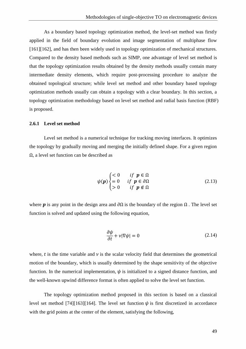
Methodologies of single-objective TO on electromagnetic devices
49
As a boundary based topology optimization method, the level-set method was firstly
applied in the field of boundary evolution and image segmentation of multiphase flow
[161][162], and has then been widely used in topology optimization of mechanical structures.
Compared to the density based methods such as SIMP, one advantage of level set method is
that the topology optimization results obtained by the density methods usually contain many
intermediate density elements, which require post-processing procedure to analyze the
obtained topological structure; while level set method and other boundary based topology
optimization methods usually can obtain a topology with a clear boundary. In this section, a
topology optimization methodology based on level set method and radial basis function (RBF)
is proposed.
2.6.1 Level set method
Level set method is a numerical technique for tracking moving interfaces. It optimizes
the topology by gradually moving and merging the initially defined shape. For a given region
Ω, a level set function can be described as
𝜓(𝒑) {
< 0 𝑖𝑓 𝒑 ∈ Ω
= 0 𝑖𝑓 𝒑 ∈ 𝜕Ω> 0 𝑖𝑓 𝒑 ∉ Ω
(2.13)
where 𝒑 is any point in the design area and ∂Ω is the boundary of the region Ω . The level set
function is solved and updated using the following equation,
𝜕𝜓
𝜕𝑡+ 𝜈|∇𝜓| = 0 (2.14)
where, 𝑡 is the time variable and 𝜈 is the scalar velocity field that determines the geometrical
motion of the boundary, which is usually determined by the shape sensitivity of the objective
function. In the numerical implementation, 𝜓 is initialized to a signed distance function, and
the well-known upwind difference format is often applied to solve the level set function.
The topology optimization method proposed in this section is based on a classical
level set method [74][163][164]. The level set function 𝜓 is first discretized in accordance
with the grid points at the center of the element, satisfying the following,

Methodologies of single-objective TO on electromagnetic devices
50
𝜓(𝑝𝑒) {< 0 𝑖𝑓 𝑥𝑒 = 1> 0 𝑖𝑓 𝑥𝑒 = 0
(2.15)
where, 𝑝𝑒 is the center of element 𝑒 in the region Ω. In order to consider the volume constraint,
the augmented Lagrangian multiplier method [164] is used here.
𝐿 = 𝜂(𝒙) + 𝜆𝑘(𝑉(𝒙) − 𝑉𝑟𝑒𝑞) +1
2Λ𝑘[𝑉(𝒙) − 𝑉𝑟𝑒𝑞]
2 (2.16)
where, 𝑘 is the iteration number, 𝜂(𝒙) is the objective function, 𝜆𝑘 and Λ𝑘 are two parameters,
which are updated using the following equation:
𝜆𝑘+1 = 𝜆𝑘 +
1
Λ𝑘(𝑉(𝒙)−𝑉𝑟𝑒𝑞)
Λ𝑘+1 = αΛ𝑘
(2.17)
where 𝛼 is a fixed constant between 0 and 1.
The velocity item 𝜈 is determined according to the gradient direction of the shape
sensitivity of the Lagrangian term 𝐿,
𝜈|𝑒 = −𝛿𝐿
𝛿Ω|𝑒
=𝛿𝜂
𝛿Ω− 𝜆𝑘 −
1
Λ𝑘(𝑉(𝒙)−𝑉𝑟𝑒𝑞) (2.18)
2.6.2 Material interpolation and RBF post-processor
As described in the previous section of SIMP-based topology optimization
methodology, the same material interpolation model is adopted to calculate the shape
sensitivity of the level set function. The general form of the model is given as below,
𝑪 = 𝑥𝑒𝑝1𝑪
0
𝒆 = 𝑥𝑒𝑝2𝒆
0
𝜺 = 𝑥𝑒𝑝3𝜺
0𝜌 = 𝑥𝑒𝜌0
(2.19)

Methodologies of single-objective TO on electromagnetic devices
51
where 𝑥𝑒 is the pseudo-density of the element; and definitions of other terms are the same as
in the previous section. It is worth noting that, different from the density variable method
before, where the design variable is a continuous value between 0 and 1, 𝑥𝑒 here takes 1 or a
small threshold value (to avoid generating singular matrices during optimization).
In order to obtain the optimized topology with a smooth boundary and make it more
suitable for industrial production, the topology optimization method based on the level set
method proposed in this section also adopts RBF-based post-processing procedure. Compared
with numerical interpolation techniques such as Lagrangian polynomial interpolation,
sequential linear interpolation and spline interpolation, RBF interpolation can still possess a
well fitted curve even with few sampling points; in addition, RBF interpolation is easy to
numerically implemented, thus helpful to facilitate a relatively automated post-processing.
The detail of RBF post-processing process is described as follows:
1. Since design variables in the proposed level set method are discrete values,
numerical instability or checkerboard phenomenon may occur in the obtained
optimized topology results. As shown in Figure 2.12(a), the initial optimized
topology obtained by the level set method contains many burrs on the edges.
Therefore, after obtaining the preliminary optimized topology, it is necessary to
first perform a post-processing to remove the scatter and fill the cavity to obtain a
smooth discrete topology containing only material or air. Here a direct mechanism
for generating a smooth discrete topology is adopted: assuming that the material
property of current element is air (or material), if at least three of its four adjacent
elements are material (or air), the material property of the current element is
changed to solid (void); Besides this condition, the material property of the
element would be not changed. At last, the discrete optimization topology is
obtained by extracting the largest connected domain, as shown in Figure 2.12(b);
2. After obtaining the discrete optimization topology, its boundary is detected, the
coordinates of the adjacent boundary nodes are calculated, and these coordinates
are regarded as a set of training samples for the radial basis function. In order to
increase the number of sample points and improve the interpolation effect of RBF,
here, the midpoint of the boundary is also counted in the training sample in
addition to the boundary endpoint, marked by the cross as shown in Figure 2.13(a);

Methodologies of single-objective TO on electromagnetic devices
52
3. The RBF approximation of the boundary is obtained by using the training sample
as an input data, and finally the smoothing boundary is reconstructed from the
RBF model just built, as shown in Figure 2.13(b).
(a) (b)
Figure 2.12 : Post-processing procedure of obtaining discrete topology.
(a) (b)
Figure 2.13 : Post-processing procedure of RBF interpolation.
2.7 Chapter summary
This chapter proposes different topology optimization methods. More specially, the
discrete topology optimization methods include the ON/OFF method, the combined Tabu-
ON/OFF method, the improved QEA based method, and the improved GA based method; a
topology optimization methodology based on SIMP and RBF, and a methodology based on
LSM and RBF are also introduced.
In the ON/OFF method, virtual materials are introduced and different annealing
mechanisms are proposed to enhance the global searching ability and improve the
convergence performance. In the combined Tabu-ON/OFF method, ON/OFF method is
combined with Tabu search algorithm. The concept of element neighborhood is introduced to
adjust to the topology optimization problem and Tabu list is removed. In the improved QEA
topology optimization method, the adaptive rotation angle is used to improve the convergence
performance. In order to reduce the computational burden, a redistribution mechanism of
design variables is designed. To further improve the global optimization ability and avoid
falling into the local optima, in the proposed improved GA method, the related concepts of
PSO algorithm are introduce and the adaptive mutation probability is adopted.
And in the SIMP-RBF based method, the continuous variation penal factor is used in
the corresponding SIMP model and the principle of RBF-post processor is explained in detail.

Methodologies of single-objective TO on electromagnetic devices
53
As for the LSM-RBF based method, discrete formulation of material interpolation model is
used, and RBF post-processing procedure is elaborated.

54
3. Methodology of multi-objective topology optimization
As stated in Chapter 1, the nature of a topology optimization problem can be regarded
as a multi-objective optimization problem; and to handle constraint conditions, in existing TO
methods like level-set method and density based method, augmented Lagrangian multiplier is
often used. By this means, the constraints and the original objective function are added
together to form a new optimization problem, which inevitably changes the characteristic of
the original problem. Besides, parameter tuning is another issue to be considered. Given all
this, a MOTO methodology based on a new hybrid MOO algorithm which integrates Non-
dominated Sorting Genetic Algorithm II (NSGAII) and Differential Evolutionary (DE) is
proposed in this chapter, the framework of the proposed algorithm is elaborated, and the
performance of the algorithm is evaluated by typical academic test functions, at last the
flowchart of the proposed methodology of MOTO is given. To be noted that, the numerical
application will be exhibited in Chapter 4.
3.1 Multi-objective optimization method
Multi-objective optimization, also called multicriteria optimization or Pareto
optimization is of an area of multiple criteria decision making, which concerns optimizing
more than one objective simultaneously using certain mathematical optimization techniques.
In most cases, these multi-objectives are conflicting with each other, no single solution exists
that can optimize all the objectives simultaneously; the optimized result is in fact a set of
trade-off and compromised solutions between different objectives. In practical life, multi-
objective optimization methods have been applied in many fields of disciplines such as
finance, economics, civil engineering, chemical process, industrial manufacturing and so on,
aiming at making best decision between two or more conflicting goals.
In order to obtatin trade-off soutions between multiple conflicing objectives, the early
methods mainly construct a new objective that can reflect the influence of multiple objectives
simultaneously by certain ways, thus converts the MOO problem into a single-objective one,
and then adopt single optimization methods to solve the problem; later, as the development of
the intelligent optimization algorithms, a variety of MOO methods based on evolutionary
algorithms have emerged, which can optimize multiple objectives at the same time.

Methodology of multi-objective topology optimization
55
3.1.1 Classical MOO method
As a priori method, a classical objective optimization method generally determines the
importance degree of each objective (linear weighted sum method) or the bound value of each
objective (constraint method) based on experience, and integrates multiple objective functions
of an optimization problem into one objective function to convert the original problem into a
single-objective optimization (SOO) one.
1. Linear weighted sum method
In solving a MOO problem using a linear weighted sum method, all the objective
functions are firstly assigned a weight by some prior knowledge or analysis of the
optimization goal, and the weighted sum of all the objectives is then to be optimized. The
weighted sum optimal method can be expressed as follows [165]:
𝑚𝑖𝑛 𝐹(𝒙) =∑𝑤𝑖𝑓𝑖(𝒙) = 𝒘 ⋅ 𝒇(𝒙)
𝑚
𝑖=1
(3.1)
where, 𝒘 = [𝑤1, 𝑤2, … , 𝑤𝑚] is the vector of weights, which satisfies,
∑𝑤𝑖 = 1
𝑚
𝑖=1
(3.2)
After a set of weight vectors is determined, the optimal solution of the original MOO
problem under as a certain linear weighted meaning is gained by solving the converted SOO
problem. By changing value of the weight vector, different Pareto solutions of the original
problem can be obtained.
2. The 휀-constraint method
In the 휀-constraint method, one “most important” objective function of the 𝑚 ones is
chosen to form a SOO problem according to the needs of the actual application or the
characteristics of the problem, and the other (𝑚 − 1) objective functions are transformed into

Methodology of multi-objective topology optimization
56
constraint conditions by setting an upper bound (or lower bound), choosing the 𝑟th objective
function to be optimized [165],
𝑚𝑖𝑛 𝑓𝑟(𝒙)
𝑠. 𝑡. 𝑓𝑖(𝒙) ≤ 휀𝑖, 1 ≤ 𝑖 ≤ 𝑚, 𝑖 ≠ 𝑟 (3.3)
where, 휀𝑖 is the upper bound constraint of the 𝑖th objective function 𝑓𝑖(𝑥) . In order to
determine the bound value of each objective function, it is usually necessary to optimize each
single objective function using some mathematical programming method. In addition, to give
decision makers more information, it is also necessary to select different values of 𝑟 and
repeat the above optimization process.
Apart from the above two typical methods, the classical MOO algorithm also include
methods such as goal programming method, goal attainment method and others. These
methods are straightforward and easy to understand. But the drawbacks are also obvious: first,
the weighted class method needs to set different weights to convert the MOO problem into a
SOO problem. The determination of reasonable weight values is the main issue. Second,
when setting the bound value of an objective, it is often necessary to optimize that objective
separately, which increases the computational cost. In summary, for the simple convex
optimization problems with prior experience, the classical MOO algorithm is simple and
effective. However, for complex non-convex MOO problems, with no prior experience given,
the classical MOO algorithm is hard to obtain satisfactory optimization results.
3.1.2 Evolutionary MOO method
In order to overcome the shortcomings and deficiencies of the above classical MOO
methods, a variety of MOO algorithms based on evolutionary algorithms are proposed.
Compared with the classical ones, evolutionary MOO algorithms optimize objective functions
by means of evolutionary intelligent algorithms like genetic algorithm simulating natural
biological evolution process, which greatly reduce the dependence on prior experience;
besides, evolutionary MOO algorithms are able to optimize multiple objective functions
simultaneously and obtain the Pareto solution set of the original MOO problem directly,
which is convenient for decision makers to collect information. Since Schaffer [166] proposed
the Vector Evaluated Genetic Algorithm (VEGA) in 1985, scholars such as Fonseca, Deb,
Horn, Zilter and Knowles have proposed fruitful different evolutionary algorithms. According

Methodology of multi-objective topology optimization
57
to the development process and characteristics of MOO evolutionary algorithms, it can be
roughly divided into three generations.
(1) First generation
The first generation began when Goldberg [167] proposed the used of non-dominated
sorting methods and niche techniques to solve MOO problems in 1989. The non-dominated
sorting method compares the advantages and disadvantages of different individuals of the
evolutionary algorithm and preserves the non-dominated individuals to enter the next
generation. This kind of survival of the fittest evolutionary thought is conducive to maintain
superior individuals, thus ensuring the global optimization ability of the algorithm; the niche
technique is mainly used to guarantee the diversity of the population, to avoid the Pareto
solution set is clustered round by a certain point. Based on these two ideas, later scholars
proposed Multi-objective Genetic Algorithm (MOGA) [168], Non-dominated Sorting Genetic
Algorithm (NSGA) [169] and Niche Pareto Genetic Algorithm (NPGA) [170].
(2) Second generation
The second generation of multi-objective evolutionary algorithms is marked by the
proposition of the Strength Pareto Evolutionary Algorithm (SPEA [171], SPEA2 [172]) using
the elitism strategy by Zitzler. The algorithm added an external population besides the
evolutionary population to preserve the non-dominated individuals (the elite solutions) in the
evolutionary process. This idea led to the evolutionary multi-objective algorithms using
different elitism strategies. Among which, there were Pareto Envelop based Selection
Algorithm (PESA [173], PESAII [174]) with an external population like in SPEA; and
without external populations, instead comparing and choosing the non-dominated individuals
between the offspring individuals and father ones like in Pareto Archived Evolution Strategy
(PAES) [175], and NSGAII [176].
Another feature of the second generation of multi-objective evolutionary algorithm is
that it no longer used the niche techniques of fitness sharing to ensure the diversity of the
algorithm, but utilized the neighbor information (NSGAII, SPEA2), introduced spatial grid
(PAES), or used region concept (PESAII) to guarantee the diversity of the population.
(3) Third generation

Methodology of multi-objective topology optimization
58
Following the prestigious NSGAII and SPEA2, which are still widely used in the field
of MOO, researchers have proposed a variety of MOO algorithms with diverse characteristics
and specialties for different problems. The third generation of multi-objective evolutionary
algorithm can roughly be divided into evolutionary pattern, dominating mechanism, high-
dimensional problem and uncertainty consideration four facets: for evolutionary pattern,
Coello et al. [177] proposed the Multi-objective Particle Swarm Optimization (MOPSO),
which used an adaptive grid mechanism to preserve the external population to make the
Pareto front more uniform, and adaptive mutation method to improve the convergence
performance. Freschi [178], Tan [179] and Gong et al. [180] applied the principle and model
of artificial immune system in MOO, respectively proposed Vector Immune System (VIS)
algorithm, Evolutionary Multi-objective Immune Algorithm (EMOIA) and Non-dominated
Neighbor Immune Algorithm (NNIA); In improving the dominance mechanism, Laumanns et
al. [181] proposed the 휀-dominance mechanism that is different from the traditional Pareto
definition. Brockoff et al. [182] proposed a partial dominance concept. Thiele [183], Zilter et
al. [184] proposed multi-objective algorithms based on preference, in the iterative process,
decision makers gave preference information to guide the evolution; To solve high
dimensional MOO problems, Wagner et al. [185] applied the aggregate function method
proposed by Hughes [186] to handle the multiple objectives in parallel. While Deb and
Saxena [187][188] used principal component analysis to extract the main objectives, abandon
redundant ones to reduce the order of the original high-dimensional problem; Aiming at
problem with uncertainties, Zhang et al. [189] used a multi-objective PSO algorithm to plan
the robot path under an uncertain environment. Mlakar et al. [190] introduced the Gaussian
process model and combined DE algorithm to consider the influence of uncertainty factors.
3.2 Basic concepts of the multi-objective optimization
Without loss of generality, a minimization MOO problem with 𝑛 decision variables
and 𝑚 objective functions can be defined as [191]
{
𝑚𝑖𝑛 𝑦 = 𝑭(𝒙) = [𝑓1(𝒙), 𝑓
2(𝒙),… , 𝑓
𝑚(𝒙)]𝑇
𝑠. 𝑡. 𝑔𝑖(𝒙) ≤ 0, 𝑖 = 1,2,… , 𝑝
ℎ𝑖(𝒙) = 0, 𝑖 = 1,2,… , 𝑞
(3.4)

Methodology of multi-objective topology optimization
59
where, 𝒙 = (𝑥1, 𝑥2, … , 𝑥𝑛) ∈ 𝑿 ⊂ 𝑅𝑛 is the decision vector of a 𝑛-dimension Euclidean space;
𝒚 = (𝑦1, 𝑦2, … , 𝑦𝑚) ∈ 𝒀 ⊂ 𝑅𝑚 is the vector of the objective function in a 𝑚dimensional
Euclidean space; 𝑭(𝒙) is a mapping of the 𝑛 dimensional decision variable space 𝑿 to the 𝑚
dimensional objective space 𝒀, i.e. 𝑭:𝑅𝑛 → 𝑅𝑚, 𝑔𝑖(𝒙) ≤ 0 and ℎ(𝒙) = 0 is respectively the
inequality constraint and the equality constraint.
3.2.1 Feasible solution and feasible solution set
The decision variable 𝒙 ∈ 𝑿 ⊂ 𝑅𝑛 for minimization problem that satisfies the
constraint conditions is called a feasible solution, and its mathematical definition is as follows.
Definition 3-1 feasible solution 𝒙 and feasible solution set 𝑿𝑓:
1. 𝒙 is a feasible solution to problem (3.4) if and only if 𝒙 satisfies all constraints of
the problem, i.e., {𝒙 ∈ 𝑅𝑛|(𝑔𝑖(𝒙) ≤ 0, 𝑖 = 1,2, … , 𝑝) ∧ (ℎ𝑖(𝒙) = 0, 𝑖 =
1,2, … , 𝑞)};
2. Let 𝑿𝑓 be a feasible solution set of problem (3.4) if and only if all 𝒙 ∈ 𝑿𝑓 ⊂ 𝑅𝑛
are feasible solutions, i.e., {∀𝒙 ∈ 𝑿𝑓 ⊂ 𝑅𝑛|(𝑔𝑖(𝒙) ≤ 0, 𝑖 = 1,2, … , 𝑝) ∧ (ℎ𝑖(𝒙) =
0, 𝑖 = 1,2, … , 𝑞)}.
3.2.2 Dominance relation and Pareto frontier
Definition 3-2 strong dominance and Pareto frontier:
Consider a system with a function 𝑭: 𝑅𝑛 → 𝑅𝑚, let 𝑿 be the compact set of feasible
solution spaces in the 𝑛 dimensional metric space, 𝒀 is the set of vectors in the 𝑚 dimensional
space, then 𝒀 = {𝒚 ∈𝑅𝑚: 𝒚 = 𝒇(𝒙) ∈ 𝑅𝑛, 𝒙 ∈ 𝑿} . Let 𝒚1 = 𝒇(𝒙1) and 𝒚2 = 𝒇(𝒙2) , among
which, 𝒚1 = (𝑦11, 𝑦12, … , 𝑦1𝑚), 𝒚2 = (𝑦21, 𝑦22, … , 𝑦2𝑚). Let 𝑴 = {1,2, … ,𝑚}, we define that
𝒚1 strictly dominates 𝒚2 (𝒚1 ≺ 𝒚2) if and only for all 𝑖 = 1,2, … ,𝑚, 𝑦1𝑖 < 𝑦2𝑖 holds, namely,
𝒚1 ≺ 𝒚2⇔ {𝑦1𝑖 < 𝑦2𝑖, ∀𝑖 ∈ 𝑴} (3.5)
It could also be written as 𝒙1 ≺ 𝒙2 . Then the corresponding non-strict dominance
concept is defined as

Methodology of multi-objective topology optimization
60
¬(𝒚1 ≺ 𝒚2) ⇔ {𝑦1𝑖 ≥ 𝑦2𝑖, ∃𝑖 ∈ 𝑴} (3.6)
The definition of Pareto frontier is then,
𝑃(𝒀) = {𝒚1 ∈ 𝒀: {𝒚2 ∈ 𝒀: 𝒚2 ≻ 𝒚1, 𝒚2 ≠ 𝒚1} = ∅} (3.7)
Definition 3-3 weak dominance and weak Pareto frontier:
Given a similar system as above, let 𝒚1 = 𝒇(𝒙1) and 𝒚2 = 𝒇(𝒙2) , among which,
𝒚1 = (𝑦11, 𝑦12, … , 𝑦1𝑚) , 𝒚2 = (𝑦21, 𝑦22, … , 𝑦2𝑚) . Let 𝑴 = {1,2, … ,𝑚} , we define that 𝒚1
weakly dominates 𝒚2 (𝒚1 ⊲ 𝒚2) if and only for all 𝑖 = 1,2, … ,𝑚, 𝑦1𝑖 ≤ 𝑦2𝑖 holds, and at least
one 𝑖 = 1,2, … ,𝑚 exists satisfying 𝑦1𝑖 < 𝑦2𝑖, namely,
𝒚1 ⊲ 𝒚2⇔ {𝑦1𝑖 ≤ 𝑦2𝑖, ∀𝑖 ∈ 𝑴}∩ {𝑦1𝑗 < 𝑦2𝑗, ∃𝑗 ∈ 𝑴} (3.8)
Also known as 𝒙1 ⊲ 𝒙2. Then the non-dominance concept is defined as
¬(𝒚1 ⊲ 𝒚2) ⇔ {𝑦1𝑖 ≥ 𝑦2𝑖 , ∃𝑖 ∈ 𝑴} ∪ {𝑦1𝑗 ≥ 𝑦2𝑗 , ∀𝑗 ∈ 𝑴} (3.9)
The definition of (weak) Pareto frontier is then,
𝑃∗(𝒀) = {𝒚1 ∈ 𝒀: {𝒚2 ∈ 𝒀:𝒚2 ⊳ 𝒚1, 𝒚2 ≠ 𝒚1} = ∅} (3.10)

Methodology of multi-objective topology optimization
61
f1
f2
A
B
CD
Figure 3.1 : Schematic diagram of Pareto dominance.
A diagram of Pareto dominance is as shown above, in which, 𝑓1(𝐷) > 𝑓1(𝐴) =
𝑓1(𝐶) > 𝑓1(𝐵), 𝑓2(𝐷) > 𝑓2(𝐶) = 𝑓2(𝐵) > 𝑓2(𝐴). From Definition 3-2, Definition 3-3, it can
be seen that point 𝐷 is strictly dominated by points 𝐴, 𝐵 and 𝐶, point 𝐴 weakly dominates
point 𝐶, point 𝐵 weakly dominates point 𝐶, and 𝐴 and 𝐵 are non-dominated by each other.
3.2.3 Performance metrics for multi-objective algorithms
For the MOO, unlike the single-objective optimization, the optimized result is not an
optimal solution but a set of solutions; meanwhile, only a finite number of Pareto solutions on
the real frontier can be obtained, and the solution sets obtained by different MOO algorithms
are generally different. Therefore, it is necessary to determine reasonable metrics to evaluate
the performance of multi-objective algorithms. The performance of an MOO algorithm is
commonly considered by both the quality of Pareto solution set and the computational cost.
The quality of a Pareto solution set is generally evaluated by the degree of closeness between
obtained Pareto frontier to true frontier and the uniformity of the distribution of the frontier;
and the computational cost is usually measured by the time required by the algorithm. The
performance metrics currently used in literature include:
(1) Number of Pareto solutions (NPS)
Give the other circumstances the same, the more number of Pareto optimal
solutions is, the stronger the searching ability of the algorithm is, and the more
information can be provided for decision makers.
(2) Ratio of Non-dominated Individuals (RNI)

Methodology of multi-objective topology optimization
62
Ratio of non-dominated individuals can be used as a metric to evaluate the
dominance of solutions between different solution sets [192], and an example of
comparison between two solution sets is given in the following. Suppose that set
𝑨 and 𝑩 are two different Pareto solution sets of the problem, and 𝑃(𝑺) represents
the set composed of all non-dominated solutions in the union set 𝑺 of 𝑨 and 𝑩,
that is,
𝑃(𝑺) = {𝒙′ ∈ 𝑺: {𝒙′′ ∈ 𝑺: 𝒙′′ ≻ 𝒙′, 𝒙′′ ≠ 𝒙′} = ∅} (3.11)
then the ratio of non-dominated individuals of set 𝑨 and set 𝑩 can be calculated as,
𝑟𝑎𝑡𝑖𝑜(𝑨) =∑ |𝒙 ∈ 𝑃(𝑺)|𝒙∈𝑨
|𝑃(𝑺)|
𝑟𝑎𝑡𝑖𝑜(𝑩) =∑ |𝒙 ∈ 𝑃(𝑺)|𝒙∈𝑩
|𝑃(𝑺)|
(3.12)
in the above, 𝒙′′ ≻ 𝒙′ indicates that solution 𝒙′′ is governed by 𝒙′, and the higher
the ratio of the non-dominated individual 𝑟𝑎𝑡𝑖𝑜(⋅) is, the higher the quality of the
solution is. Since NRI indicator does not have closeness under sum operation,
generally ratio(𝑨) + ratio(𝑩) ≠ 1 . When comparing the quality of multiple
solution sets, NRI metric is very intuitive to evaluate and the quality of each
solution set.
(3) Convergence metric - Υ
The convergence metric [176] reflects the proximity of the obtained non-
dominated frontier 𝑄 and the real Pareto frontier 𝑃∗. The smaller the value of Υ is,
the closer the non-dominated frontier of the algorithm is to the real frontier,
namely the better the convergence of the algorithm is.
Υ =∑ 𝑑𝑖𝑁𝑄𝑖=1
𝑁𝑄 (3.13)
where 𝑑𝑖 is the closest distance between the 𝑖th non-dominated solution and the
real Pareto frontier. 𝑁𝑄 stands for the number of non-dominated solutions in
Pareto frontier obtained by the algorithm.
(4) Diversity metric - Δ
Diversity metric [176] reflects the distance between neighboring points in a non-
dominated solution set 𝑄 , and describes the degree of uniformity of the
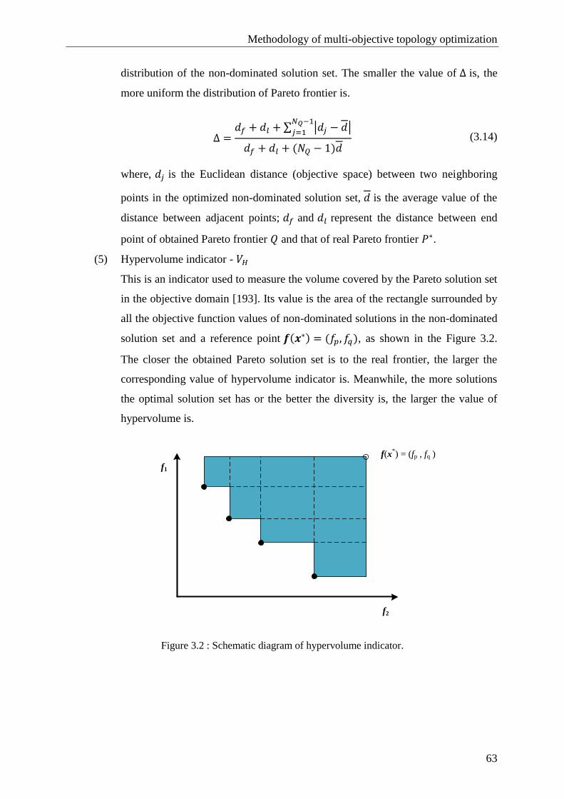
Methodology of multi-objective topology optimization
63
distribution of the non-dominated solution set. The smaller the value of Δ is, the
more uniform the distribution of Pareto frontier is.
Δ =𝑑𝑓 + 𝑑𝑙 + ∑ |𝑑𝑗 − 𝑑|
𝑁𝑄−1
𝑗=1
𝑑𝑓 + 𝑑𝑙 + (𝑁𝑄 − 1)𝑑 (3.14)
where, 𝑑𝑗 is the Euclidean distance (objective space) between two neighboring
points in the optimized non-dominated solution set, 𝑑 is the average value of the
distance between adjacent points; 𝑑𝑓 and 𝑑𝑙 represent the distance between end
point of obtained Pareto frontier 𝑄 and that of real Pareto frontier 𝑃∗.
(5) Hypervolume indicator - 𝑉𝐻
This is an indicator used to measure the volume covered by the Pareto solution set
in the objective domain [193]. Its value is the area of the rectangle surrounded by
all the objective function values of non-dominated solutions in the non-dominated
solution set and a reference point 𝒇(𝒙∗) = (𝑓𝑝, 𝑓𝑞), as shown in the Figure 3.2.
The closer the obtained Pareto solution set is to the real frontier, the larger the
corresponding value of hypervolume indicator is. Meanwhile, the more solutions
the optimal solution set has or the better the diversity is, the larger the value of
hypervolume is.
f1
f2
f(x*) = (fp , fq )
Figure 3.2 : Schematic diagram of hypervolume indicator.

Methodology of multi-objective topology optimization
64
3.3 A new hybrid multi-objective optimization algorithm
Although the NSGAII proposed by Deb [176] and the SPEA2 proposed by Zitler [172]
enjoy a reputation in the field of multi-objective optimization, numerical experiments have
demonstrated that when binary coded NSGAII and SPEA2 are used to find the Pareto frontier
of some typical multi-objective test functions, their performance is not ideal. Considering that
the essence of the topology optimization problem is the problem of determining material
distribution of the optimization region, and after the discretization using finite element
method, the design domain can naturally be regarded as a binary encoded chromosome;
therefore the evolutionary search algorithm is very natural and convenient to be applied.
Based on this observation, we propose a multi-objective topology optimization methodology
based on a hybrid algorithm which integrates binary encoded NSGAII and DE.
First of all, a large number of literatures have shown that the NSGAII is simple in
structure, easy to be implemented, and has strong global search ability. Therefore, the
NSGAII is chosen as the main algorithm in the proposed hybrid one and a new mutation
operator is introduced to update the population. In this way, the main component being the
NSGAII can guarantee that the proposed hybrid algorithm has good global search ability.
Secondly, to further enhance the global optimization ability of the binary encoded
NSGAII so as to avoid the algorithm to fall into local optima, a mutation operator is
introduced in the hybrid algorithm.
In addition, theoretical studies and numerical experiments show that despites that
binary NSGAII has strong global optimization ability, nevertheless, when dealing with
complex multi-objective optimization problems, the number of non-dominated solutions in
the Pareto frontier is sometimes insufficient. The distribution of the final solutions may also
be uneven. In order to find more non-dominated solutions and make the Pareto frontier
distribution more uniform, the binary DE is integrated. The DE algorithm was proposed and
improved by R. Storn and K. Price [194]. The algorithm is simple, fast, and robust. The main
idea of the algorithm is to generate new individuals by performing differential operations on
different individuals in the population. Based on this, the hybrid algorithm applies the
differential evolution strategy to the elite archive, which enhances the local refinement ability
of the algorithm, and thus improves the uniformity of the non-dominated frontier obtained by
the algorithm.

Methodology of multi-objective topology optimization
65
Finally, NSGAII itself does not have the elite archive, the hybrid algorithm sets the
elite archive solution set with reference to the SPEA2, and updates the so far found non-
dominated solutions by continuously maintaining the elite archive; at the same time, uses
differential evolution strategy in the elite archive to generate new solutions.
3.3.1 Improved NSGA
The iterative steps of the NSGAII are briefly explained as:
1) Initialize the population size 𝑝𝑜𝑝𝑠𝑖𝑧𝑒, the maximum number of iterations 𝑀𝑎𝑥𝐼𝑡
and related parameters;
2) Randomly generating an initial population 𝑃0 and calculating the objective
function value of each individual;
3) For the individuals in the initial population 𝑃0, a population is 𝑄0 generated by
tournament selection, crossover and mutation, objective function values of the
individuals in population 𝑄0 is calculated, and an iteration counter 𝑡 = 0 is set;
4) Let 𝑅𝑡 = 𝑃𝑡 ∪ 𝑄𝑡, all individuals in 𝑅𝑡 are non-dominated sorted according to the
objective function values of individuals, and the crowding distance of each
individual is calculated. All the individuals are then divided into different non-
dominated front ends 𝐹 = (𝐹1, 𝐹2, … , 𝐹𝑖, … ) according to the dominance between
them. Find the value i of front-end which satisfies the expression |𝐹1| + ⋯+
|𝐹𝑖−1| < 𝑝𝑜𝑝𝑠𝑖𝑧𝑒 ≤ |𝐹1| + ⋯+ |𝐹𝑖|, and sort all the individuals according to the
crowding distance;
5) All the individuals in 𝐹1, 𝐹2, … , 𝐹𝑖−1 are copied into the population 𝑃𝑡+1, and the
first 𝑝𝑜𝑝𝑠𝑖𝑧𝑒 − ∑ |𝐹𝑚|𝑖−1𝑚=1 individuals in Fi are copied to the population 𝑃𝑡+1, as
shown in Figure 3.3;
6) For individuals in population 𝑃𝑡+1 , a new population 𝑄𝑡+1 is generated by
tournament selection, crossover and mutation;
7) If 𝑡 > 𝑀𝑎𝑥𝐼𝑡, the algorithm terminates, and all non-dominated solutions in 𝑃𝑡 are
output as optimization results; otherwise, let 𝑡 = 𝑡 + 1, go to step 4).

Methodology of multi-objective topology optimization
66
Rt
Pt
Qt
Pt+1
Front set
F1
F4
F3
F2
Fn
Individuals to be eliminated
Figure 3.3 : Population updating process in NSGAII.
1. Non-dominated sorting and crowding distance calculation
Non-dominated sorting is the core of the NSGAII. It selects the superior individuals in
the population to enter the next generation of population. The detailed procedures are
described as follows:
1) The number of being dominated 𝑛𝑝 of all the individuals 𝑝 in population 𝑃 is
initialized to 0, and the dominating set 𝑆𝑝 is initialized to an empty set. Among
which, the number 𝑛𝑝 is used to record the number of individuals in population 𝑃
that dominate 𝑝, and the set 𝑆𝑝 is used to store the individuals in population 𝑃 that
are dominated by 𝑝;
2) Compare any two individuals in the population 𝑃 , update the corresponding
number of being dominated and dominating set of each individual, move the
individuals with the dominated number 𝑛𝑝 = 0 into the non-dominated front end
𝐹𝑖, and set the non-dominated front end counter 𝑖 = 1;
3) Accessing each solution 𝑞 in dominating set 𝑆𝑝 of the non-dominated front end 𝐹𝑖,
and for solution 𝑞, set the number of being dominated 𝑛𝑞 = 𝑛𝑞 − 1. Set a new
population 𝑄, if 𝑛𝑞 = 0, then 𝑄 = 𝑄 ∪ 𝑞 ;
4) If population 𝑄 is not empty, then let 𝑖 = 𝑖 + 1 , copy the individuals in the
population 𝑄 to the non-dominated front end 𝐹𝑖 , and go to step 3). Repeat the
above process until all the non-dominated fronts are determined.

Methodology of multi-objective topology optimization
67
Non-dominated sorting divides the individuals in a population into different front ends.
For individuals at the same front end, it is necessary to sort by calculating and comparing the
crowding distance. The crowding distance measures the intensity around the individual in the
population. After the crowding distance is sorted, NSGAII algorithm preferentially selects the
individuals with fewer surrounding individuals, namely, individuals with large crowding
distance is preferred, so that the optimized Pareto front can have a uniform distribution.
The crowding distance 𝐷𝑖𝑠𝑡𝑎𝑛𝑐𝑒(𝑝) of individual 𝑝 is defined as follows:
𝐷𝑖𝑠𝑡𝑎𝑛𝑐𝑒(𝑝) =∑|𝑓𝑖(𝑝 + 1) − 𝑓𝑖(𝑝 − 1)|
(𝑓𝑖𝑚𝑎𝑥 − 𝑓𝑖
𝑚𝑖𝑛)⁄
𝑚
𝑖=1
(3.15)
where, 𝑚 is the number of objective functions for optimization, 𝑓𝑖(𝑝 + 1) and 𝑓𝑖(𝑝 − 1) are
respectively the values of objective function of two neighboring individuals corresponding to
the individual . For an individual on the boundary, namely, one of its objective function
values is the largest or smallest among all the individuals, which as shown in the Figure 3.4,
the crowding distance of individual 𝐵 at the boundary is set to positive infinity.
f1
f2
p
p-1
p+1
Inf
B
B
Figure 3.4 : Calculation of crowding distance.
2. Selection, crossover and mutation procedures
NSGAII algorithm primarily generates new population from superior individuals
through selection, crossover, and mutation operations. In the improved NSGAII, a tournament
selection method is used. First, an individual 𝑠 is randomly selected from the population and a

Methodology of multi-objective topology optimization
68
random integer 𝑡𝑜𝑢𝑟 is generated. Repeat 𝑡𝑜𝑢𝑟 times to select another individual 𝑠′ from the
population 𝑃𝑡. If 𝑠′ dominates 𝑠, then let 𝑠′ = 𝑠. This process is repeated 𝑚 times to obtain a
population 𝑅𝑡 containing 𝑚 individuals. For all individuals in the population 𝑅𝑡 , each two
pairs are cross-operated according to the crossover probability to obtain a new population 𝑈𝑡;
then all individuals in the population 𝑈𝑡 are mutated according to the mutation probability to
obtain a new population 𝑄𝑡.
It should be noted that the crossover operation adopted here is crossed based on the
dimension of the variable, that is, the binary bit string under the same variable dimension of
the parent individual is cross-operated; and the mutation operation is to uniformly mutate the
chromosomes under all variable dimensions according to the mutation probability.
Parent individual
Child individual
1 0 0 1... 1 0 11 00 0 1 1 1 1 0 00... ... ...
1 0 0 11 0 10 00 0 1 1 1 1 0 01... ... ... ...
Mutation
... ... ... .........
variable 1p1 pDp2q1 q2 qD
Parent 1
1 1 1 0 001 0 0 11 0 11 00 0 1
... ... ... ......... 0 0r1 rD
0r2s1 s2 sD
011 0 1 010 0 01 11 0 1
Parent 2variable 2 variable D
variable 1 variable 2 variable D
Crossover
... ... ... .........
... ... ... .........
r1 rDr2s1 s2
1 1 1 0 00sD
p1 pDp2q1 q2 qD
Child 1
Child 2
0 0 01 11 0 1
1 0 11 00 0 1 1 0 0 1
0 0 0 1 011 0 1 0
variable 1 variable 2 variable D
variable 1 variable 2 variable D
Figure 3.5 : Crossover and mutation operation in improved NSGAII.
In the field of biology, DNA was initially thought to be stable and unchanged. Until
the late 1960s, scientists succeeded in extracting jumping genes from bacteria and calling
them transposons. Later, the role of transposons in the resistance of bacteria to antibodies has
gradually become known. Almost simultaneously, studies have found that transposons can
also produce genetic variation (diversity) in natural populations. These extra chromosomal
transposons are not essential for normal life, but they can confer properties such as resistance
and toxicity, providing survival advantages under the certain conditions. In fact, nearly 20%
of an organism's genome may contain transposons [195].

Methodology of multi-objective topology optimization
69
The proposed mutation operator mimics the way in which transposon variation occurs
in natural genetics, adopting an insertion and substitution method. Define the mutation
probability of the jump gene operation is 𝑃𝑗𝑢𝑚𝑝 , and the individuals in the population are
sequentially mutated by the jump gene operator according to the probability 𝑃𝑗𝑢𝑚𝑝. As shown
in Figure 3.6, two positions 𝑝 and 𝑞 on the original binary chromosomal bit strings are
randomly generated, and the chromosomes in the middle of the two positions are replaced
with random binary bit strings of the same length.
Jumping-gene operator
Original chromosome
Transposonr s
Chromosome with
jumping genesr s
p q
r s
10 0 0 0 1
p q
1 0 0 01 1... ...
0 0 1 00 1... ...
r s
Figure 3.6 : Jumping gene mutation operator.
The improved NSGAII algorithm (hereafter referred to as JNSGA) preserves the non-
dominated sorting of NSGAII, the calculation of crowding distance, and the genetic
operations of selection, crossover and mutation. However, the elite retention strategy of
NSGAII reduces the diversity of population to some extent. Inspired by jumping genes (or
transposons) in biology, this hybrid algorithm introduces jumping gene mutation operator to
increase the population diversity: thereby improving the overall global search ability of the
algorithm.
3.3.2 Binary DE algorithm
In order to deal with the issue of binary coding in the topology optimization problem,
it is necessary to handle the continuous variables in the original DE algorithm. The commonly
used methods for the discretization of continuous variable in binary DE algorithms are
rounding and mapping transformation. The rounding method limits the variables to 0~l, and
rounds off to get 0 or 1 discrete variable; the mapping transformation method, with reference
to binary particle swarm optimization (BPSO) algorithm uses a secondary search space, using
a surjection to convert the variable to the discrete field {0,1}𝑛 . The first method obtains

Methodology of multi-objective topology optimization
70
discrete variables by rounding, which has low coding efficiency and affects the search
performance of the algorithm; the second mapping method needs to introduce other functions
to convert continuous variables into discrete ones, and the numerical experiments show that
this method is undesirable. In this regard, a parameter-free binary mutation operator [196] is
used to form a binary DE algorithm. The mutation operator can directly generate the mutation
vector without the variation parameter, and the details are as follows:
𝑣𝑖,𝑗𝑡 = 𝑥𝑟1,𝑗
𝑡 + (−1)𝑥𝑟1,𝑗𝑡
⋅ |𝑥𝑟2,𝑗𝑡 − 𝑥𝑟3,𝑗
𝑡 |
𝑗 = 1,2,… ,𝐷 (3.16)
where 𝑖 represents the 𝑖th individual of the mutated population, 𝑗 represents the dimension of
variables, 𝑡 is the number of the current iteration; 𝑥𝑟1𝑡 , 𝑥𝑟2
𝑡 and 𝑥𝑟3𝑡 are three individuals
different from each other in the population.
Since the value of the variable in the topology optimization is only 0 or 1, the absolute
value of the vector difference is also only 0 or 1. It can be seen from the (3.16) that the
variable obtained after the mutation is still a 0-1 variable, thus the operation satisfies the
closeness. In the variation procedure, whether a certain dimensional variable is mutated
depends on the value of the difference vector. When the absolute value of the 𝑗th component
in the difference vector (𝒙𝒓𝟐𝒕 − 𝒙𝒓𝟑
𝒕 ) is 1, namely |𝑥𝑟2,𝑗𝑡 − 𝑥𝑟3,𝑗
𝑡 | = 1, the corresponding base
vector component is mutated (from 0 to 1, or from 1 to 0), to increase the diversity of the
population, improve the global search ability of the algorithm, prevent falling into the local
optima; when the absolute value |𝑥𝑟2,𝑗𝑡 − 𝑥𝑟3,𝑗
𝑡 | = 1, 𝑥𝑟1,𝑗𝑡 remains unchanged, which is good
for retaining the information of superior individuals and speeding up the convergence of the
algorithm.
The basic flowchart of the BDE algorithm is as follows:
1) Randomly generate popsize D-dimensional vectors as the initial population,
𝒙𝒊𝒕 = {𝑥𝑖,1
𝑡 , 𝑥𝑖,2𝑡 , … , 𝑥𝑖,𝐷
𝑡 }, 𝑖 = 1,2, … , 𝑝𝑜𝑝𝑠𝑖𝑧𝑒 ;
2) Binary parameter-free mutation operator. The variation is carried out bitwise by
randomly selecting three different individuals in the population;

Methodology of multi-objective topology optimization
71
𝒗𝒊𝒕 = 𝒙𝒓𝟏
𝒕 + (−1)𝒙𝒓𝟏𝒕⋅ |𝒙𝒓𝟐
𝒕 − 𝒙𝒓𝟑𝒕 | (3.17)
3) Crossover operation. As a supplement to the mutation operator, DE algorithm
retains part of the information of the individual 𝒙𝒊𝒕, and generates the individuals
of child 𝒖𝒊𝒕 = 𝑢𝑖,1
𝑡 , 𝑢𝑖,2𝑡 , … , 𝑢𝑖,𝐷
𝑡 , the specific steps are:
𝑢𝑖,𝑗𝑡 = {
𝑣𝑖,𝑗𝑡 , 𝑖𝑓 𝑟𝑎𝑛𝑑 < 𝐶𝑅 𝑜𝑟 𝑗 = 𝑗𝑟𝑎𝑛𝑑
𝑥𝑖,𝑗𝑡 , 𝑜𝑡ℎ𝑒𝑟𝑤𝑖𝑠𝑒
(3.18)
where 𝐶𝑅 is the crossover probability; 𝑗𝑟𝑎𝑛𝑑 is a random integer from 1 to D.
4) Selection operation. Use the greedy principle to compare the parent and the
offspring, the individuals with the best objective function values constitute the
next generation of the population;
5) Terminating condition judgment. If the number of the current iteration 𝑡 exceeds
the maximum evolution iteration number 𝑡𝑚𝑎𝑥 , the search is stopped and the
optimization result is output; otherwise, returning to step 2), the loop is continued.
The proposed binary DE algorithm adopts a parameter-free binary mutation operator,
which can directly perform binary mutation according to the difference between individuals.
The structure is simple and easy to be implemented. The advantages of DE algorithm relying
on the population differences for evolution are well preserved at the same time. By analyzing
the evolutionary strategies and characteristics of the real-coded DE algorithm, it can be
concluded that the differential operation in the proposed binary DE evolutionary algorithm
finds better individuals to evolve by refining the search in the space around the elite solutions.
The crossover operation partially retains the information of the original individual and the
mutated individual enhances the diversity of the population. This local refinement capability
is just needed to be enhanced by the original NSGA.
3.3.3 Flowchart of the proposed algorithm
Based on the improved NSGAII and BDE algorithm, a new hybrid multi-objective
optimization algorithm, JNSGA-DE, is proposed. To introduce the binary DE algorithm, the
hybrid algorithm sets up the elite solution set 𝐴𝑟𝑐ℎ𝑖𝑣𝑒 and continuously updates the

Methodology of multi-objective topology optimization
72
individuals in the 𝐴𝑟𝑐ℎ𝑖𝑣𝑒 in the iterations. The search strategy of the hybrid algorithm is:
JNSGA explores the whole search space to ensure that the algorithm has a good global search
ability; the DE algorithm acts on the current elite solution set 𝐴𝑟𝑐ℎ𝑖𝑣𝑒 , searches in the
vicinity of the currently found optimal solutions, to enhance the local refinement search
ability of the hybrid algorithm. The flowchart of the algorithm is shown in Figure 3.7.
Start
Non-dominated sorting and crowding distance caculation
Initialization of Archive
Tournament selection to
choose parent individuals
Crossover and mutation operation
Random selection in Archive to
choose parent individuals
Binary parameter-free muation
Jumping gene operator Crossover operator
Initialization of population
Generate mixed population
Maintenance of Archive
Greedy strategy to update the population
Stop criterion
Stop
JN
SG
A p
roce
du
re DE
pro
cedu
re
Non-dominated sorting and crowding distance caculation
Figure 3.7 : Flowchart of the proposed hybrid algorithm JNSGA-DE.
1. Greedy strategy

Methodology of multi-objective topology optimization
73
The hybrid algorithm uses a greedy strategy to update the population, that is, the
individuals in the mixed population of JNSGA and DE are ranked by using non-dominated
sorting and crowding distance. The lower the value of non-dominated front end (in Section
3.3.1) is and the larger crowding distance is, the better the individual’s rank is. Select the top
ranked 𝑝𝑜𝑝𝑠𝑖𝑧𝑒 individuals to form the next generation of populations. By using the greedy
strategy, the genetic information closer to the real frontier is preserved, helping to speed up
the convergence of the algorithm.
2. Maintenance of archive
Archive is used as an evolutionary population of the DE algorithm on the one hand
and storage of non-dominated solutions to output the final optimization result on the other
hand. In the hybrid algorithm, the size of the Archive changes dynamically; as shown in
Figure 3.7, in each iteration, after the new population is generated, it is compared with the
original elite solutions, and the non-dominated solutions are selected to become the Archive
of the next generation. The upper limit of the number of solutions in Archive is set to the size
of the population.
3.4 Algorithm performance analysis and validation
3.4.1 Test functions
In order to test the performance of the proposed JNSGA-DE hybrid algorithm and
compare it with the existing renowned multi-objective optimization algorithms, it is used to
solve the standard test functions as given in [176] and [197]. The characteristics of these test
functions and their Pareto Frontiers (PF) are tabulated in Table 3.1.
Table 3.1 : Test functions
𝑓(⋅) n Domain Objective function Solution PF
SCH 1 [−103, 103] {𝑓1(𝑥) = 𝑥
2
𝑓2(𝑥) = (𝑥 − 2)2 𝑥 ∈ [0, 2] convex
FON 3 [−4, 4]
{
𝑓1(𝑥) = 1 − 𝑒𝑥𝑝 [−∑(𝑥𝑖 −
1
√3)23
𝑖=1
]
𝑓2(𝑥) = 1 − 𝑒𝑥𝑝 [−∑(𝑥𝑖 +1
√3)23
𝑖=1
]
𝑥1 = 𝑥2 = 𝑥3
[−1
√3,1
√3]
non-
convex
POL 2 [−𝜋, 𝜋] {𝑓1(𝑥) = 1 + (𝐴1 − 𝐵1)
2 + (𝐴2 − 𝐵2)2
𝑓2(𝑥) = (𝑥1 + 3)2 + (𝑥2 + 1)
2 ref
non-
convex
discont
inuous

Methodology of multi-objective topology optimization
74
KUR 3 [−5, 5]
{
𝑓1(𝑥) = ∑ [−10𝑒𝑥𝑝 (−0.2√𝑥𝑖
2 + 𝑥𝑖+12 )]
𝑛−1
𝑖=1
𝑓2(𝑥) = ∑(|𝑥|0.8 + 5 sin 𝑥𝑖3)
𝑛
𝑖=1
ref
non-
convex
discont
inuous
ZDT1 30 [0, 1] {
𝑓1(𝑥) = 𝑥1
𝑓2(𝑥) = 𝑔(𝑥) [1 − √𝑥1𝑔(𝑥)
]
𝑔(𝑥) = 1 + 9(∑𝑥𝑖
𝑛
𝑖=2
) (𝑛 − 1)⁄
𝑥1 ∈ [0, 1]
𝑥𝑖≠1 = 0𝑖 = 2,… , 𝑛
convex
ZDT2 30 [0, 1]
{
𝑓1(𝑥) = 𝑥1
𝑓2(𝑥) = 𝑔(𝑥) [1 − (𝑥1𝑔(𝑥)
)2
]
𝑔(𝑥) = 1 + 9(∑𝑥𝑖
𝑛
𝑖=2
) (𝑛 − 1)⁄
𝑥1 ∈ [0, 1]
𝑥𝑖≠1 = 0𝑖 = 2,… , 𝑛
non-
convex
ZDT3 30 [0, 1] {
𝑓1(𝑥) = 𝑥1
𝑓2(𝑥) = 𝑔(𝑥) [1 − √𝑥1𝑔(𝑥)
−𝑥1𝑔(𝑥)
⋅ sin(10𝜋𝑥1)]
𝑔(𝑥) = 1 + 9(∑𝑥𝑖
𝑛
𝑖=2
) (𝑛 − 1)⁄
𝑥1 ∈ [0, 1]
𝑥𝑖≠1 = 0𝑖 = 2,… , 𝑛
convex
discont
inuous
ZDT4 10
𝑥1 ∈ [0, 1]
𝑥𝑖≠1 ∈ [−5, 5]
𝑖 = 2,… , 𝑛
{
𝑓1(𝑥) = 𝑥1
𝑓2(𝑥) = 𝑔(𝑥) [1 − √𝑥1𝑔(𝑥)
]
𝑔(𝑥) = 1 + 10(𝑛 − 1) +∑[𝑥𝑖2 − 10 cos(4𝜋𝑥𝑖)]
𝑛
𝑖=2
𝑥1 ∈ [0, 1]
𝑥𝑖≠1 = 0𝑖 = 2,… , 𝑛
non-
convex
ZDT6 10 [0, 1]
{
𝑓1(𝑥) = 1 − 𝑒𝑥𝑝(−4𝑥1)sin6(6𝜋𝑥1)
𝑓2(𝑥) = 𝑔(𝑥) [1 − (𝑓1(𝑥)
𝑔(𝑥))
2
]
𝑔(𝑥) = 1 + 9(∑𝑥𝑖
𝑛
𝑖=2
(𝑛 − 1)⁄ )
0.25
𝑥1 ∈ [0, 1]
𝑥𝑖≠1 = 0𝑖 = 2,… , 𝑛
non-
convex
uneven
distrib
ution
Note: in the table, n represents the dimension of the optimization problem, and in the objective
function of POL optimization problem,
𝐴1 = 0.5 sin1 − 2 cos 1 + sin2 − 1.5 cos2𝐴2 = 1.5 sin1 − cos 1 + 2sin 2 − 0.5 cos 2𝐵1 = 0.5 sin 𝑥1 − 2cos 𝑥1 + sin 𝑥2 − 1.5 cos 𝑥2𝐵2 = 1.5 sin 𝑥1 − cos𝑥1 + 2sin 𝑥2 − 0.5 cos𝑥2
3.4.2 Algorithm verification
1. Test counterparts
In order to verify the performance of the hybrid algorithm, the well-known multi-
objective evolutionary algorithms, NSGAII and SPEA2, are used as comparison counterparts.

Methodology of multi-objective topology optimization
75
NSGAII and SPEA2 are programmed according to the relevant literatures. MATLAB
platform is used for programming implementation and relevant parameters are set according
to the literatures.
Table 3.2 : Algorithm parameters in JNSGA-DE, NSGAII and SPEA2
@ 8 G RAM, 3.4GHz
CPU
Hybrid NGSAII SPEA2
popsize 100
100
100
MaxIt 250 250 250
pc 0.9 0.9 0.8
pm 1 𝑛⁄ 1 𝑛⁄ 1 𝑛⁄
pjump 0.7
CR 0.5
Size of Archive 100
100
Note: in the table, n is the length of the chromosome. For instance, if the number of
design variables is 10, and 30 binary bits are used for each variable, then the length of
chromosome is 300.
2. Performance indicators
To evaluate the performance of an algorithm, each algorithm is performed 30
independent runs on each test function for a statistical comparison. The performance
indicators of multi-objective algorithms have been described previously, and two statistical
analysis indicators are adopted in this section. The first one is the convergence metric Υ,
which is used to characterize the distance between the PF frontier obtained by the algorithm
and the true PF frontier of the test function; and the second one is the diversity metric Δ,
which indicates the uniformity of the distribution of the PF frontier solution obtained by the
optimization algorithm, namely, the diversity. The calculation method of the above
performance indicators is detailed in section 3.2.3.
The smaller the convergence metric Υ is, the closer is the final solution of an algorithm
to the true PF frontier, that means the better the convergence performance of the algorithm is;
the diversity metric Δ reflects the space between adjacent solutions. The smaller the metric is,
the more uniform the distribution is. For the test functions listed in the table, there are infinite
points on the true frontier. For the convenience of calculation, 500 pairs of uniform sampling
points on the true frontier are used to represent the true PF.

Methodology of multi-objective topology optimization
76
The two indicators obtained by 30 independent runs of each algorithm are statistically
analyzed to evaluate the statistical average performance of the algorithm. Mean values 𝐸(Υ),
𝐸(Δ), and standard deviations 𝜎(Υ), 𝜎(Δ) of the indicator Υ, Δ are respectively used. The
above mean value and standard deviation reflect the value and distribution stability in the
statistical sense, respectively. Therefore, they can be used to evaluate the overall performance
of the algorithm.
3. Optimization indicator analysis
The optimization results of the three algorithms JNSGA-DE, NSGAII and SPEA2 for
different test functions are shown in Table 3.3 and Table 3.4. Table 3.3 compares the
convergence indicator of the three algorithms, and Table 3.4 shows the comparison of the
diversity indicator. For each algorithm, the mean value and standard deviation of the
corresponding indicators when optimizing different test functions are analyzed statistically.
(1) Convergence indicator analysis
a) Comparing JNSGA-DE algorithm with the NSGAII, only in the SCH test
function, the convergence value of the later is slightly smaller than the former, and
only the difference of 4 digits after the decimal point; on the other test functions,
the convergence indicator of the JNSGA-DE algorithm are better than that of the
NSGAII, especially for the ZDT1, ZDT2, ZDT3, ZDT4, and ZDT6 test functions,
the optimization result of JNSGA-DE is much better than the NSGAII. Not only
the statistical mean value of the convergence indicator is smaller, but also the
standard deviation is smaller, that means the stability of the former algorithm is
better.
b) Compared with the SPEA2, the JNSGA-DE only has a larger mean value of the
convergence indicator in ZDT2. On the other test functions, the mean and
standard deviation of the convergence indicator of the JNSGA-DE algorithm are
better, especially for the ZDT4 function (this function has 219 local optima in the
whole decision space, and therefore has higher requirement for the global
optimization ability of the algorithm), the convergence indicator of the former is
much better than that of the latter.
c) It can be seen from the optimization results of the convergence indicator that
the overall convergence of the JNSGA-DE is better than the NSGAII and SPEA2

Methodology of multi-objective topology optimization
77
algorithms: that is, the optimized Pareto frontier is closer to the true frontier. At
the same time, the JNSGA-DE algorithm is more stable and more reliable.
Table 3.3 : Comparison of statistical results of the convergence indicator
𝑓(⋅) JNSGA-DE NSGAII SPEA2
𝐸(Υ) 𝜎(Υ) 𝐸(Υ) 𝜎(Υ) 𝐸(Υ) 𝜎(Υ)
SCH 0.0033 𝟓. 𝟗𝟒 × 𝟏𝟎−𝟓 𝟎. 𝟎𝟎𝟑𝟐 1.72 × 10⁻⁴ 0.0033 2.65 × 10⁻⁴
FON 𝟎. 𝟎𝟎𝟐𝟏 𝟎. 𝟎𝟎𝟏𝟖 0.0074 0.0058 0.0052 0.0035
POL 𝟎. 𝟎𝟏𝟔𝟖 𝟎. 𝟎𝟎𝟏𝟐 0.0347 0.0346 0.0255 0.0210
KUR 𝟎. 𝟎𝟏𝟐𝟓 𝟖. 𝟖𝟖 × 𝟏𝟎−𝟒 0.0749 0.1438 0.0505 0.1361
ZDT1 𝟎. 𝟎𝟏𝟗𝟎 𝟎. 𝟎𝟎𝟒𝟗 0.1786 0.0711 0.0382 0.0171
ZDT2 0.0761 𝟎. 𝟎𝟐𝟑𝟏 0.5118 0.1776 𝟎. 𝟎𝟔𝟒𝟒 0.0316
ZDT3 𝟎. 𝟎𝟎𝟗𝟓 𝟎. 𝟎𝟎𝟏𝟗 0.0710 0.0346 0.0120 0.0046
ZDT4 𝟎. 𝟑𝟗𝟎𝟐 𝟎. 𝟐𝟐𝟑𝟔 5.6711 2.1459 8.4953 4.8732
ZDT6 𝟎. 𝟏𝟗𝟎𝟏 𝟎. 𝟏𝟐𝟑𝟗 1.4942 0.7083 0.3088 0.1309
(2) Diversity indicator analysis
a) Compared with the NSGAII, the JNSGA-DE algorithm has better statistical
performance of the diversity indicator on all test functions, especially for the
ZDT series problems, the advantage is obvious; while on ZDT2, ZDT4 and
ZDT6 problem, NSGAII has smaller standard deviation of the diversity
indicator.
b) Compared with the SPEA2, for the statistical mean value of the diversity
indicator, JNSGA-DE is better than SPEA2 on all test functions; SPEA2 has
smaller standard deviation on the ZDT2, ZDT4 and ZDT6 problems. On the
other test functions, hybrid algorithm has better performance.
c) According to the optimization results of the diversity indicator, although the
stability index of the hybrid algorithm is slightly worse (the standard
deviation is slightly larger) on the ZDT2, ZDT4 and ZDT6, the uniformity of
the Pareto solution obtained by the JNSGA-DE algorithm is better overall, the
optimized Pareto frontier is more uniform.

Methodology of multi-objective topology optimization
78
Table 3.4 : Comparison of statistical results of the diversity indicator
𝑓(⋅) JNSGA-DE NSGAII SPEA2
𝐸(Δ) 𝜎(Δ) 𝐸(Δ) 𝜎(Δ) 𝐸(Δ) 𝜎(Δ)
SCH 𝟎. 𝟑𝟔𝟏𝟐 𝟎. 𝟎𝟎𝟖𝟒 0.4430 0.0350 0.8311 0.0891
FON 𝟎. 𝟐𝟗𝟎𝟔 𝟎. 𝟎𝟑𝟎𝟎 0.4867 0.0700 0.4336 0.0910
POL 𝟎. 𝟗𝟒𝟕𝟓 𝟎. 𝟎𝟏𝟕𝟓 0.9654 0.0245 1.0285 0.0415
KUR 𝟎. 𝟒𝟎𝟏𝟕 𝟎. 𝟎𝟐𝟒𝟖 0.5538 0.0570 0.6154 0.0598
ZDT1 𝟎. 𝟑𝟒𝟓𝟒 𝟎. 𝟎𝟗𝟏𝟐 0.7495 0.1833 0.6389 0.1068
ZDT2 𝟎. 𝟔𝟗𝟒𝟖 0.2564 1.0171 𝟎. 𝟏𝟒𝟕𝟐 0.7013 0.1820
ZDT3 𝟎. 𝟔𝟔𝟑𝟏 𝟎. 𝟎𝟕𝟕𝟔 0.8913 0.1361 0.9039 0.0832
ZDT4 𝟎. 𝟔𝟒𝟔𝟓 0.1313 0.9219 0.0440 0.9693 𝟎. 𝟎𝟐𝟒𝟕
ZDT6 𝟎. 𝟔𝟑𝟎𝟏 0.1240 1.0606 𝟎. 𝟎𝟕𝟔𝟎 0.9720 0.0955
SCH test function
0 1.0 2.0 3.0 4.00
1.0
2.0
3.0
4.0
1st objective – f1
2nd o
bje
ctiv
e –
f2
JNSGA-DETrue PF
FON test function
0 0.2 0.4 0.6 0.8 1.00
0.2
0.4
0.6
0.8
1.0
1st objective – f1
2nd o
bje
ctiv
e –
f2
JNSGA-DETrue PF
POL test function
0 3.0 6.0 9.0 12.0 15.0 18.0 0
5.0
10.0
15.0
20.0
25.0
2n
d o
bje
ctiv
e – f
2
1st objective – f1
JNSGA-DETrue PF
KUR test function
-20.0 -19.0 -18.0 -17.0 -16.0 -15.0 -14.0-12.0
-10.0
-8.0
-6.0
-4.0
-2.0
0
2nd o
bje
ctiv
e – f
2
1st objective – f1
JNSGA-DETrue PF
ZDT1 test function ZDT2 test function

Methodology of multi-objective topology optimization
79
2nd o
bje
ctiv
e – f
2
1st objective – f1
0 0.2 0.4 0.6 0.8 1.00
0.5
1.0JNSGA-DETrue PF
0 0.2 0.4 0.6 0.8 1.00
0.2
0.4
0.6
0.8
1.0
1.2
2n
d o
bje
ctiv
e – f
2
1st objective – f1
JNSGA-DETrue PF
ZDT3 test function
0 0.2 0.4 0.6 0.8 1.0-1.0
-0.5
0
0.5
1.0
1st objective – f1
2n
d o
bje
ctiv
e –
f2
JNSGA-DETrue PF
ZDT4 test function
1st objective – f1
0 0.2 0.4 0.6 0.8 1.00
0.2
0.4
0.6
0.8
1.0
2n
d o
bje
ctiv
e –
f2
JNSGA-DETrue PF
ZDT6 test function
1st objective – f1
0.2 0.3 0.4 0.5 0.6 0.7 0.8 0.9 1.0
0
0.2
0.4
0.6
0.8
1.0
1.2
2n
d o
bje
ctiv
e – f
2
JNSGA-DETrue PF
Figure 3.8 : Optimization results of different test functions by JNSGA-DE.
4. Conclusion
The optimization results of the test functions demonstrate that the proposed JNSGA-
DE hybrid algorithm effectively combines the advantages of NSGAII and DE. By introducing
the jump gene mutation operator, the global search ability of NSGAII is further enhanced. At
the same time, the introduction of the DE algorithm effectively improves the distribution

Methodology of multi-objective topology optimization
80
uniformity of the obtained non-dominated solutions. For the 9 test functions with different
Pareto frontier features, the hybrid algorithm has strong global and local search ability,
especially for the ZDT4 test function with a large number of local optima, the performance of
the hybrid algorithm is much better than those of the NSGAII and SPEA2.
3.5 A multi-objective topology optimization methodology
Based on the proposed hybrid MOO algorithm, a MOTO methodology is constructed.
The flowchart of the TO method is presented in Figure 3.9. The whole optimization process
can be explained as below,
JNSGA-DE evolution
Start
Create initial topologies
Initialization
FEM analysis
Output optimization results
Termination criterion
satisfied
Generate new topologies
Figure 3.9 : Flowchart of the proposed MOTO methodology
1. Variables are declared, storage memory is prepared, and relevant parameters are
set;
2. The population is randomly sampled to generate initial topologies;

Methodology of multi-objective topology optimization
81
3. Finite element analysis is carried out to calculate the values of multiple objectives
corresponding to each topology;
4. New topologies are generated by executing the evolution process proposed in
JNGSA-DE algorithm;
5. Check if termination criterion is satisfied;
6. The optimization is terminated and meanwhile the MOTO results are output.
3.6 Chapter summary
This chapter first briefly reviews multi-objective optimal algorithms; introduces the
related terminologies, the fitness assignment, and enumerates several common performance
indicators for evaluating multi-objective algorithms. A hybrid algorithm–JNSGA-DE by
integrating NSGA and DE algorithms is then proposed. The jumping gene mutation and DE
evolution strategy in the hybrid algorithm are explained in detail. The performance of the
hybrid algorithm is tested on 9 test functions with different Pareto frontier distributions. And
in the end, a multi-objective topology optimization methodology is proposed.
The numerical results of academic test functions indicate that the proposed hybrid
algorithm has good global and local searching ability. Especially in the cases of non-convex
and uneven distributed Pareto frontiers (such as ZDT4 and ZDT6), the performance of the
proposed algorithm is better than those of NSGAII and SPEA2. Considering that the actual
electromagnetic topology optimization design problem is mostly non-convex, the introduction
of the constraint may make the Pareto frontier of the objective function space unevenly
distributed. Therefore, the proposed multi-objective topology optimization methodology is
quite suitable for the topology optimization design of electromagnetic devices.

82
4. Numerical applications
4.1 Case study 1 : single-objective topology optimization
Electromagnetic actuators convert electrical and mechanical energy one into another.
The energy conversion takes place in the so-called air gap separating the stationary part
(stator or fixed contact) and moving part (rotor or moving contact) of the actuator. It is widely
used in the mechanical manufacturing industry from precise control using small actuators to
the quite large powerful units using electrical drives. Therefore, it is quite meaningful to
optimize the topological shape of the electromagnetic actuator to improve its performance by
using a topology optimization technology. In this chapter, the proposed ON/OFF method, the
combined Tabu-ON/OFF method, the improved QEA method and the improved GA topology
optimization method are applied to the topology optimization of a prototype electromagnetic
actuator. The optimization goal of this study is to maximize the electromagnetic force of the
armature in a specified direction by optimizing the topology under a fixed input power.
Figure 4.1 : An electromagnetic actuator [198].

Numerical applications
83
4.1.1 Solid model
The initial geometry of an electromagnetic actuator commonly used in engineering
applications is shown in Figure 4.2, which utilizes an iron core surrounded by electrified coils
to attract the armature or hold a mechanical workpiece in a fixed position. The armature and
the core are ferromagnetic material and the relative magnetic permeability of the armature is
2000 and that of the core is 1000. The core is wound by a coil of 1A current with 420 turns.
The air gap between the armature and the right end of the core is fixed at 2 mm. The design
domain of the electromagnetic actuator is shown in Figure 4.3.
Armature
Coil (+)
Coil (-)
Core
42
5
9
30
12
10
2
8
Unit: mm
Figure 4.2 : Initial geometry of the electromagnetic actuator.
Desig
nD
om
ain
Figure 4.3 : Design domain of the electromagnetic actuator.

Numerical applications
84
4.1.2 Mathematical formulation
The actuating force is determined using a virtual magnetic energy method from the
finite element solution. Therefore, the mathematical model for the magnetic actuator topology
optimization can be formulated as [64]:
𝑀𝑎𝑥𝑖𝑚𝑖𝑧𝑒 𝐹 = −𝜕𝑊𝑚𝑎𝑔𝑛𝑒𝑡𝑖𝑐
𝜕𝑥
𝑆𝑢𝑏𝑗𝑒𝑐𝑡 𝑡𝑜 ∑ 𝑉𝑒 < 𝑉𝑖𝑛𝑖𝑡𝑖𝑎𝑙
𝑁
𝑒=1
(4.1)
where 𝑉𝑒 is the volume of each element, 𝑁 is the number of the total elements of magnetic
material in the design domain. 𝑉𝑖𝑛𝑖𝑡𝑖𝑎𝑙 is the volume of the design domain in the initial model.
4.1.3 Numerical results
1. ON/OFF method
For the sensitivity analysis, adjoint variable methods can generally be used [42][199].
However, the forward finite difference approximation is used in this paper for versatility:
𝑑𝐹
𝑑𝑝= lim
∆𝑝→0
∆𝐹
∆𝑝≈𝐹(𝑝 + ∆𝑝)−𝐹(𝑝)
∆𝑝 (4.2)
where 𝑝 is the design variable (here is the permeability of an element) and ∆𝑝 represents the
perturbation of 𝑝. The performance parameter 𝐹 is computed by using finite element analysis.
Under the previous conditions, a prototype magnetic actuator is optimized using the
proposed methodology. To demonstrate the performances of different annealing mechanisms,
the proposed methodologies using different annealing mechanisms and strategies, Traditional
ON/OFF method (Traditional), Strategy 1 under the annealing mechanism A (Strategy 1_A),
Strategy 2 under the annealing mechanism A (Strategy 2_A), Strategy 3 under the annealing
mechanism A (Strategy 3_A), Strategy 4 under the annealing mechanism A (Strategy 4_A),
and the annealing mechanism B, other conditions being equal, are experimented on this case
study. The optimized topology is shown in Figure 4.4 and Figure 4.5 depicts the

Numerical applications
85
corresponding magnetic flux lines. The optimized results and performances of the
methodology in different annealing strategies and mechanisms are given in Table 4.1. The
trajectory of the absolute value of the objective function is shown in Figure 4.6.
X
Y
Z
Figure 4.4 : Optimized topology by ON/OFF-finite difference method.
Optimized topologyInitial topology
Figure 4.5 : Magnetic flux lines of initial and optimized topology.
Table 4.1 : Comparison of objective function using different annealing mechanisms
Annealing mechanism Objective function (N/m) CPU time (s)
Traditional -49.22 9385.783
Strategy 1_A -52.90 10153.509
Strategy 2_A -52.90 10138.097
Strategy 3_A -52.90
10178.531
Strategy 4_A -52.90 9637.734
Mechanism B -52.90 5842.414

Numerical applications
86
0 5 10 15 20 25 30 35
0
10
20
30
40
50
60
Iteration
Abso
lute
val
ue
of
obje
ctiv
e fu
nct
ion (
N/m
)
Traditional
Mechansim AMechanism B
Figure 4.6 : Trajectory of objective function.
From the numerical results, it can be observed that,
a) The actuating forces for the initial and optimized topologies are, respectively,
42.67 and 52.90 (𝑁 𝑚⁄ ). In other words, the magnetic force is increased about 24%
compared to that of the initial design, while the magnetic material consumption is
small.
b) The finally optimized objective function using different strategies are almost the
same, but are all better than the results using traditional ON/OFF method. And the
CPU time used under the annealing mechanism B is tremendously reduced, about
60%, compared to those using other annealing strategies. To intuitively explain
these results, Figure 4.6 shows the convergence trajectories of the objective
function using different annealing mechanisms. It is observed that the finally
optimized objective functions using mechanism A and mechanism B are the same
and keep unchanged after some number of generations (10 for this case study).
However, the iterative procedure using mechanism A will continue because the
number of changeable elements is greater than 1. On the contrary, the iterative
procedures under the annealing mechanism method B will be immediately
stopped since the material attribute is not changed for consecutive 7 iterations.
And to some extent, the setting of parameter α is reasonable.
2. The combined Tabu-ON/OFF method

Numerical applications
87
The proposed combined Tabu-ON/OFF topology optimization method is applied to
this case study, and the related materials and parameter settings are the same as the previous
section. The optimized topology is shown in Figure 4.7, Figure 4.8 depicts the distribution of
magnetic lines corresponding to the original design and the optimized topology. The
trajectory of the objective function value in the optimization process is shown in Figure 4.9.
Figure 4.7 : Optimized topology by Tabu-ON/OFF method.
Initial topology Optimized topology
Figure 4.8 : Magnetic flux lines of initial and optimized topology.
0 10 20 30 40 50 60 70 80 90 100 1100
10
20
30
40
50
60
Iteration
Ab
solu
te v
alu
e o
f o
bje
ctiv
e fu
nct
ion
Figure 4.9 : Trajectory of objective function.

Numerical applications
88
From these numerical results, it can be see that, after the topology optimization, the
electromagnetic force of the armature is significantly increased despite of the reduced use of
magnetic material in core; Comparing with the initial design, the electromagnetic force is
increased about 25% from 42.67 to 53.16 𝑁 𝑚⁄ . As shown in Figure 4.8, the optimized
magnetic field lines are more concentrated in the vicinity of the armature under optimized
topology design, which is why the electromagnetic force of the armature is increased. Figure
4.9 reveals the good convergence of the proposed algorithm, that is, as the optimization
process goes on, better values of the objective function are continuously found. However, it
can be seen from the convergence curve that the algorithm is also easy to stagnate near local
optimal points, which proves that the adoption of the reset mechanism in the algorithm, using
a counter to determine whether the method is stagnant into local optimal, is reasonable and
reliable.
3. The improved QEA
The prototype of the electromagnetic actuator is also optimized by using the proposed
topology optimization method based on improved quantum evolution algorithm (QEA). In
order to evaluate the performance of the improved QEA and verify the proposed design
variable redistribution mechanism (RM), in this section four different methods, namely, the
original quantum evolution algorithm (noted as OQ), the improved quantum evolution
algorithm (IQ), and the original QEA with variable redistribution mechanism (OQ with RM)
and the improved QEA with the variable redistribution mechanism (IQ with RM) are
employed to optimize the topology of the electromagnetic actuator, and the obtained
numerical results are compared. Table 4.2 shows the objective function, the number of
iterations, and the time consumed by different methods. In the cases of the variable
redistribution mechanism, the corresponding objective function value of each optimization
step is listed. The optimized topology obtained by the original QEA and the improved QEA
methods are shown in Figure 4.10 and Figure 4.11 respectively, and Figure 4.12 describes the
trajectories of the objective function. For the cases of the design variable redistribution
mechanism, Figure 4.13 shows the optimized topology result corresponding to each step using
the original QEA with the variable redistribution mechanism; and Figure 4.14 exhibits the
optimized topology of each step by using the improved QEA algorithm with the variable
distribution mechanism. Figure 4.15 depicts stepwise optimization trajectory of the objective
function of the original QEA method and the improved QEA method using the variable

Numerical applications
89
redistribution mechanism. In these results, OQ step1 stands for the first step of the original
QEA algorithm; similarly, IQ step3 represents the third step of the improved QEA.
To facilitate the illustration of the selection of variables when adopting the design
variable redistribution mechanism, Figure 4.16 shows the selection of design variables in the
design domain for each step using improved QEA method. In Figure 4.16, the yellow color on
the left side of each optimization step is the design variable, and the right side is the optimized
topology corresponding to this step.
Table 4.2 : Optimization results comparison of original QEA and revised QEA
Method Objective function (N/m) Iteration number CPU time(s)
OQ -54.74 3000 110078.37
IQ -54.91 2900 107843.47
OQ with RM -51.54 -54.72 -54.95 1800 61679.10
IQ with RM -51.54 -54.89 -54.95 1600 58682.19
Figure 4.10 : Optimized topology of the original QEA.
Figure 4.11 : Optimized topology of the revised QEA.

Numerical applications
90
0 500 1000 1500 2000 2500 3000
Iteration
0
10
20
30
40
50
60
Ab
solu
te v
alu
e of
ob
ject
ive
fun
ctio
n
OQEARQEA
Figure 4.12 : Objective function trajcetories of the original and revised QEA.
Step 1
Step 2
Step 3
Figure 4.13 : Optimized topology of each step in the original QEA with RM.

Numerical applications
91
Step 1
Step 2
Step 3
Figure 4.14 : Optimized topology of each step in the revised QEA with RM.
0 200 400 600 800 1000 1200 1400 1600 1800
Iteration
10
15
20
25
30
35
40
45
50
55
5
Ab
solu
te v
alu
e o
f o
bje
ctiv
e fu
nct
ion
OQ step1OQ step2OQ step3
RQ step2RQ step3
RQ step1
Figure 4.15 : Objective function trajectory of each step by adopting the RM.

Numerical applications
92
Design variable and
optimization result in Step 1
Design variable and
optimization result in Step 2
Design variable and
optimization result in Step 3
Figure 4.16 : Selection of design variables in each step and corresponding optimized topology.
From these numerical results, it can be seen that
a) The objective function value corresponding to the optimized topology by the
traditional QEA algorithm is 54.74 (𝑁 𝑚⁄ ), and the objective function value
corresponding to the improved QEA algorithm is 54.91. Using the design variable
redistribution mechanism, the objective function values in the first, the second and
third step of the original QEA, are 51.54, 54.72 and 54.95 respectively; while the
objective function value in the first, the second and the third step of the revised
QEA are 51.54, 54.89 and 54.95 respectively. Considering that the objective
function under the original design is 42.67 (𝑁 𝑚⁄ ), the electromagnetic force is
eventually increased about 28.8% by using the improved QEA with RM, and at
the same time, the material cost is reduced.
b) The objective function value of the improved QEA is larger than that of the
traditional QEA method. And meanwhile, it can be seen from the optimized
topology in Figure 4.10 and Figure 4.11 that there are cavities in the optimized
topology obtained by the original QEA algorithm, and the optimized topology
obtained by the improved QEA algorithm has no this checkerboard issue.
Therefore, it can be concluded that the former's global search ability is better than
the latter.
c) The number of iterations in Table 4.2 refers to the number of iterations when the
algorithm finds the optimal topology (the maximum value of the objective
function). It can be observed from the table that the improved QEA algorithm
converges slightly faster than the original QEA algorithm; the variable
redistribution mechanism will reduce greatly the number of design variables for
each step, so that the number of iterations required per step is greatly reduced. The

Numerical applications
93
computation time consumed is approximately half of the time required for the
case when redistribution mechanism is unemployed.
d) As can be seen from the objective function trajectory of Figure 4.12 and Figure
4.15, the objective function value of the improved QEA is slightly smaller than
the original QEA algorithm at the beginning of the search process, but as search
continues, the value of the improved QEA is gradually larger than that of the
original QEA, which also demonstrates that the global search ability of the
improved QEA algorithm is stronger, and it is less likely to be trapped into the
local optimal solutions as compared to the original QEA.
4. The improved GA
The proposed improved GA in Chapter 2.4 is finally applied to the topology
optimization of the electromagnetic actuator. In the numerical implementation, the topology
of a prototype magnetic actuator is optimized using different methods for performance
comparison. The methods include the traditional ON/OFF method (T_ON/OFF), the merely
improved ON/OFF method (I_ON/OFF), the merely improved GA (I_GA), and the proposed
hybrid method (ON/OFF_GA). Figure 4.17, Figure 4.18, Figure 4.19 and Figure 4.20 depict,
respectively, the optimized topology of the traditional ON/OFF method, the improved
ON/OFF method, the improved GA and the hybrid method. The corresponding performances
are compared in Table 4.3.
X
Y
Z
Figure 4.17 : Optimized topology by the traditional ON/OFF method.

Numerical applications
94
X
Y
Z
Figure 4.18 : Optimized topology by the improved ON/OFF method.
Figure 4.19 : Optimized topology by the improved GA method.
X
Y
Z
Figure 4.20 : Optimized topology by the ON/OFF-GA hybrid method.
Table 4.3 : Optimization results comparison of different methods
Optimization method Objective function(N/m) CPU time (s)
T_ON/OFF -49.22 9385.783
I_ON/OFF -52.90 5842.414
I_GA -54.94 36699.565

Numerical applications
95
ON/OFF_GA -54.91 31870.162
From these numerical results, it is observed that:
a) The objective functions are 49.22 (𝑁 𝑚⁄ ) under the optimized topology of
ON/OFF method, 52.90 (𝑁 𝑚⁄ ) under the optimized topology of improved
ON/OFF method, 54.94 under the optimized topology of I_GA, and 54.91 under
the optimized topology of ON/OFF_GA method. Considering the actuating force
of the initial topology of 42.67 (𝑁 𝑚⁄ ), the magnetic force can be increased about
29% and the magnetic material consumption is nearly 74% under the optimized
topologies of I_GA method and GA_ON/OFF topology optimization methodology.
b) The proposed I_ON/OFF method outperforms T_ON/OFF. The absolute value of
the objective function of the former is larger than that of the latter, which is
mainly contributed by the introducing of virtual material. The convergence is
faster since new a new annealing strategy is proposed.
c) The optimized results of I_GA and ON/OFF_GA are better than those of
T_ON/OFF and I_ON/OFF, validating that the global searching ability of
methodologies is increased by adopting improved GA.
d) The final solution of I_GA and ON/OFF_GA are merely the same while the CPU
time used by the former is about 1.15 times of the latter.
4.2 Case study 2 : single-objective topology optimization
Micro-electromechanical systems (MEMS) have a wide range of applications in
remote and embedded systems due to their miniaturization and good adaptability.
Piezoelectric energy recovery (PEH) device, as one of the MEMSs that converts mechanical
vibrational energy to electrical energy, shows great potential in remote sensors and embedded
devices due to its compact size [16][18][20]. When a piezoelectric energy harvester device is
subjected to external vibration, the upper and lower surfaces of the piezoelectric material will
generate a potential difference. In this section, the topology optimization methodologies based
on the SIMP method the level set method are applied to optimize the topology of a
piezoelectric energy harvester (PEH), and then be verified.

Numerical applications
96
4.2.1 Solid model
Figure 4.21 is a schematic diagram of a cantilever piezoelectric energy harvester
model. The whole system consists of substrate, piezoelectric layer, electrodes and load. The
left side surface of the base and the piezoelectric layer and are applied fixed constraints. The
upper and lower surface of the piezoelectric layer is respectively set as equipotential surface
condition, and electrodes are added on the two surfaces (the influence of the introduction of
electrodes on the model is ignored here), and the external load is connected between the two
electrodes. Under external mechanical vibration, voltage will be generated on the
piezoelectric material layer of the PEH, and two electrodes respectively connected to the
upper and lower surfaces of the piezoelectric layer will generate a potential difference.
electrode 1
electrode 2
fixed
constraint
Load
piezoelectric
material
substrate
mechanical
force
Figure 4.21 : Schematic of piezoelectric energy harvester model.
1. Objective function
To evaluate the performance of the piezoelectric energy harvesting devices, an energy
conversion factor is introduced. The energy generated by an external force 𝐹 is stored in the
strain energy Π𝑆 and the electric energy Π𝐸 , which are defined as:
Π𝑆 =1
2𝒖𝑇𝑲𝑢𝑢𝒖
Π𝐸 =1
2𝝋𝑇𝑲𝜑𝜑𝝋
(4.3)

Numerical applications
97
The topology optimization of the piezoelectric energy harvester is thus formulated as
𝑀𝑎𝑥𝑖𝑚𝑖𝑧𝑒 𝜂 =Π𝐸
Π𝐸 +Π𝑆
𝑠. 𝑡. ∑ 𝛾𝑒𝑣𝑒 < 𝑉0
𝑁
𝑒=1
0 < 𝛾𝑒 ≤ 1, 𝑒 ∈ [1,𝑁]
(4.4)
where 𝑣𝑖 denotes the volume of the 𝑖𝑡ℎ element, 𝑁 is the number of the finite elements in the
design domain. 𝑉0 is a given upper bound volume constraint and is set 60% of the design
domain.
2. Finite element formulation
In this study, a 3D finite element model of piezoelectric energy harvester is developed
to analyze the performance. Electrodes are deposited on the piezoelectric part and imposed
equipotential electrical conditions. The influence of the electrodes in mechanic is neglected.
In the static case, the external is an open circuit and the bottom surface of the piezoelectric
material layer is equipotential grounding. The coupled mechanical and electric finite element
formulation under the static case is thus given as
𝑲𝑢𝑢𝑼+𝑲𝑢𝜑𝚽 = 𝑭
𝑲𝜑𝑢𝑼−𝑲φφ𝚽 = 𝑸 (4.5)
where 𝑲𝑢𝜑 represents the piezoelectric coupling matrix; 𝑲𝑢𝑢 and 𝑲𝜑𝜑 denote the structural
stiffness and dielectric conductivity matrices; 𝑼 and 𝚽 denote displacement and electrical
potential vectors; 𝑭 and 𝑸 are the applied force and electric charge vectors, respectively.
For the harmonic case, the above equation can be formulated as
𝑴𝑢𝑢�̈� + 𝑲𝑢𝑢𝑼+𝑲𝑢𝜑𝚽 = 𝑭
𝑲𝜑𝑢𝑼−𝑲𝜑𝜑𝚽 = 𝑸 (4.6)

Numerical applications
98
where 𝑴𝑢𝑢 is the structural mass matrix; �̈� denotes the displacement acceleration vectors.
Considering the structural damping, Rayleigh damping is added to the above matrix. Electric
circuits are described by using the equivalent capacitance matrix method [200] and the
resultant matrices are compromised into the dielectric matrix. Equation (4.6) can thus be
formulated as
𝑴𝑢𝑢�̈� + 𝑪𝑢𝑢�̇� + 𝑲𝑢𝑢𝑼+𝑲𝑢𝜑𝚽 = 𝑭
𝑲𝜑𝑢𝑼− (𝑲𝜑𝜑 + �̂�𝜑𝜑)𝚽 = 𝐐 (4.7)
where 𝑪𝑢𝑢 is the damping matrix; �̂�𝜑𝜑 is the effective capacitance matrix. In both the static
and harmonic case, as the applied electric charge is zero, 𝑸 is always zero.
3. Sensitivity analysis
Sensitivity information of the objective function with respect to the design variables is
computed to bias iterative process. From (4.4), the first order derivative of the objective
function is formulated as
𝜕𝜂
𝜕𝛾𝑒=
𝜕Π𝐸𝜕𝛾𝑒
(Π𝐸 +Π𝑆)−Π𝐸 (𝜕Π𝐸𝜕𝛾𝑒
+𝜕Π𝑆𝜕𝛾𝑒
)
(Π𝐸 +Π𝑆)2
(4.8)
According to (4.3), 𝜕Π𝐸
𝜕𝛾𝑒 and
𝜕Π𝑆
𝜕𝛾𝑒 can be written as
𝜕Π𝐸𝜕𝛾𝑒
=1
2
𝜕𝝋𝑇
𝜕𝛾𝑒𝑲𝜑𝜑𝝋+
1
2𝝋𝑇𝜕𝑲𝜑𝜑𝜕𝛾𝑒
𝝋+1
2𝝋𝑇𝑲𝜑𝜑
𝜕𝝋
𝜕𝛾𝑒
𝜕Π𝑆𝜕𝛾𝑒
=1
2
𝜕𝒖𝑇
𝜕𝛾𝑒𝑲𝑢𝑢𝒖+
1
2𝒖𝑇𝜕𝑲𝑢𝑢𝜕𝛾𝑒
𝒖+1
2𝒖𝑇𝑲𝑢𝑢
𝜕𝒖
𝜕𝛾𝑒
(4.9)
By the convenience of introducing the material interpolation model, 𝜕𝐊𝑢𝑢
𝜕𝛾𝑒, and
𝜕𝐊𝜑𝜑
𝜕𝛾𝑒
can be easily obtained. As for partial derivative 𝜕𝒖
𝜕𝛾𝑒 and
𝜕𝛗
𝜕𝛾𝑒, the adjoint matrix method is
employed by solving the following equation:

Numerical applications
99
[
𝑲𝑢𝑢 𝑲𝑢𝜑
𝑲𝜑𝑢 −𝑲𝜑𝜑
]
[ 𝜕𝒖
𝜕𝛾𝑒
𝜕𝝋
𝜕𝛾𝑒]
= −
[ 𝜕𝑲𝑢𝑢𝜕𝛾𝑒
𝜕𝑲𝑢𝜑𝜕𝛾𝑒
𝜕𝑲𝜑𝑢𝜕𝛾𝑒
−𝜕𝑲𝜑𝜑𝜕𝛾𝑒 ]
[
𝒖
𝝋] (4.10)
It should be noted that, the above equations are valid only for the sensitivity analysis
under static case. For the harmonic case, equation (4.3) is adjusted to
Π𝑆∗ =
1
2�̅�𝑇𝑲𝑢𝑢𝒖
Π𝐸∗ =
1
2�̅�𝑇𝑲𝜑𝜑𝝋
(4.11)
where �̅� is the conjugate vector of displacement vector 𝒖, and �̅� is the conjugate vector of
electrical potential vector of 𝝋. Moreover, according to (4.7), the coupled mechanical and
electric finite element equation under the harmonic case can be given as
[
𝑲𝑒𝑓𝑓 𝑲𝑢𝜑
𝑲𝜑𝑢 −𝑲𝜑𝜑∗] [𝑼
𝚽] = [
𝑭
𝑸] (4.12)
where 𝑲𝑒𝑓𝑓 and 𝑲𝜑𝜑∗ is respectively the following equation,
𝑲𝑒𝑓𝑓 = −𝜔2𝑴𝑢𝑢 + 𝑗𝜔𝑪𝑢𝑢 +𝑲𝑢𝑢
𝑪𝑢𝑢 = 𝛼𝑴𝑢𝑢 + 𝛽𝑲𝑢𝑢
(4.13)
𝑲𝜑𝜑∗ = 𝑲𝜑𝜑 + �̂�𝜑𝜑 (4.14)
And then, the adjoint equation for sensitivity analysis can formulated be

Numerical applications
100
[
𝑲𝑒𝑓𝑓 𝑲𝑢𝜑
𝑲𝜑𝑢 −𝑲𝜑𝜑∗]
[ 𝒖
𝜕𝛾𝑒
𝜕𝝋
𝜕𝛾𝑒]
= −
[ 𝜕𝑲𝑒𝑓𝑓𝜕𝛾𝑒
𝜕𝑲𝑢𝜑𝜕𝛾𝑒
𝜕𝑲𝜑𝑢𝜕𝛾𝑒
−𝜕𝑲𝜑𝜑
∗
𝜕𝛾𝑒 ]
[
𝒖
𝝋] (4.15)
As for the derivative of the objective function, the equation can be composed
accordingly based on (4.8) and (4.9).
4.2.2 Mathematical formulation
1. Static case
In the static case, the optimal piezoelectric material distribution of a unimorph energy
harvester under static point load is considered, as shown in Figure 4.22. The whole structure
is composed of substrate, piezoelectric material and mass proof. An external force is applied
to the middle point of the mass proof. The arrows on the piezoelectric plate show the
polarization direction of the piezoelectric materials. Two electrodes placed on the top and
bottom surfaces of the piezoelectric material. The entire piezoelectric material layers are set
as the design domain. The design variables of top, middle and bottom layers are treated as the
same along the z-direction in one hand to prevent the complex or impractical porous topology.
The top and bottom layers of the piezoelectric material are equipotential boundary condition
and the bottom layer is grounded. Finite element model and sensitivity analysis are in Chapter
4.2.1; the objective is to maximize the conversion factor subject to a volume constraint where
the usage of piezoelectric material is limited to up to 60%.

Numerical applications
101
electrode 1
electrode 2
Design domain
z
y
x
F = 0.1N
0
1
0 1 1
N
e e
e
e
Maximize
s.t. v V
, e ,N
Figure 4.22 : Problem defination of static case.
2. Harmonic case
In this case, an optimization problem under a harmonic body force load is considered.
An external body force loading is applied to the whole structure as shown in Figure 4.23. The
FE discretization is the same as that in the static case. The piezoelectric layer is set as the
design domain. The upper bound of the volume constraint is set to be 60%. The first-order
eigen frequency of the whole system with an initial design, is calculated from a numerical
analysis, is 202.89 𝐻𝑧. Consequently, the excitation frequency is set to be 200 𝐻𝑧 and value
of the resistor of external circuit is 500 𝑘Ω.
electrode 1electrode 2
z
y
x
a = 0.1g
1
0 1
N
e e req
e
e e
Maximize
s.t. x v V
x or x
electrode 1
electrode 2Resistor
Figure 4.23 : Problem defination of harmonic case.
4.2.3 Numerical results
1. The SIMP method

Numerical applications
102
Based on the finite element formulation, the solid model of piezoelectric energy
harvester is analyzed. In this study case, the topology of design domain is optimized
respectively under the static condition and the harmonic one. And the optimized topology
under different working condition is obtained. The numerical results are validated by using
FEA software COMSOL.
(1) Static case
First, three combinations of the penalization factors- [𝑝1 𝑝2 𝑝3] are compared. For the
first two combinations, the penalization factors are fixed constants; for the third one, 𝑝1 is set
to be continuous varied according to (2.10). For easiness of demonstration of the optimized
topology, a vertical view of the initial optimized topology by using SIMP is given in Figure
4.24. The objective function trajectories using different penalization factors are plotted in
Figure 4.25. The solid line represents the objective function value and the dotted line denotes
the maximum density change between two neighboring iterations. From Figure 4.24 and
Figure 4.25, it can be observed that different combinations of the penalization factors will
produce different topologies even though the objective function values are close. However,
the density variation in the continuous penalization factor case is the smallest. The updating
process of the element density is steady to proceed. From this perspective, the convergence
performance of the optimization is improved by adopting the proposed continuously varied
penalization factor mechanism.
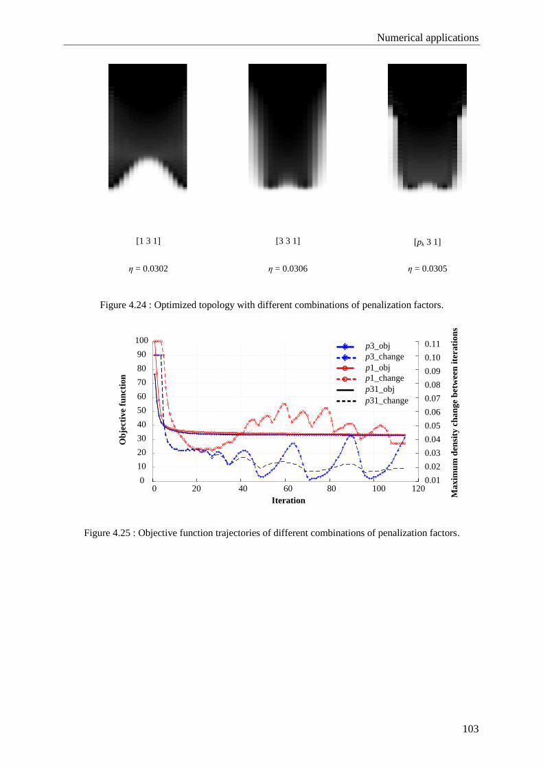
Numerical applications
103
[pk 3 1][1 3 1] [3 3 1]
η = 0.0302 η = 0.0306 η = 0.0305
Figure 4.24 : Optimized topology with different combinations of penalization factors.
Ma
xim
um
den
sity
ch
an
ge
bet
wee
n i
tera
tio
ns
Ob
ject
ive
fun
ctio
n
0
10
20
30
40
50
60
70
80
90
100
0 20 40 60 80 100 120
0.01
p3_obj
p3_change
p1_obj
p31_obj
p1_change
p31_change
0.05
0.03
0.02
0.04
0.06
0.09
0.08
0.07
0.11
0.10
Iteration
Figure 4.25 : Objective function trajectories of different combinations of penalization factors.

Numerical applications
104
(a) (b) (c)
Figure 4.26 : Optimization results of static case.
Figure 4.26 also presents the blurry topology (a) obtained by the SIMP method, the
discrete topology (b) after binarization and the smoothed topology (c) after adopting the RBF
post-processor.
(2) Harmonic case
The optimized topology under the harmonic case is given in Figure 4.27.
(a) (b) (c)
Figure 4.27 : Optimization results of harmonic case.
To validate the performance of the proposed methodology, both the static and the
harmonic optimization results are validated using the commercial FEA software COMSOL.
The elastic energy, electric energy and energy conversion factor in the initial design, the
obtained discrete topology and the smoothed topology are given in Table 4.4 and Table 4.5.
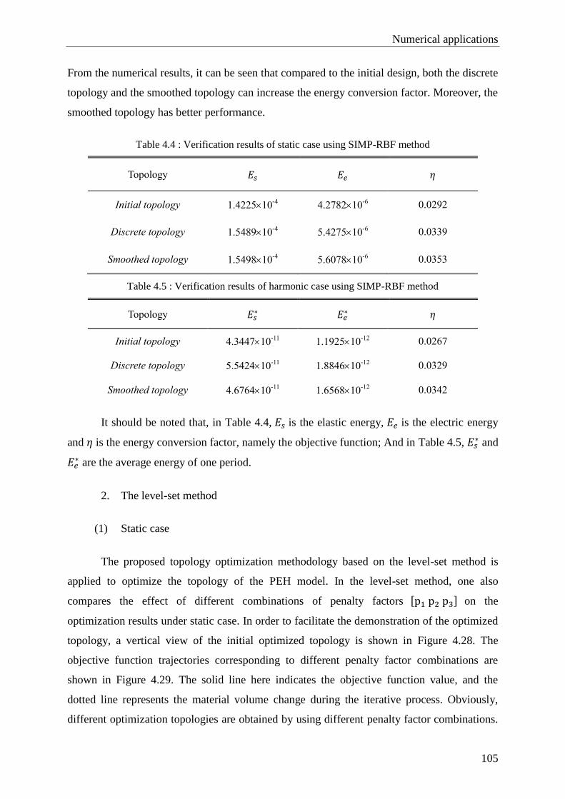
Numerical applications
105
From the numerical results, it can be seen that compared to the initial design, both the discrete
topology and the smoothed topology can increase the energy conversion factor. Moreover, the
smoothed topology has better performance.
Table 4.4 : Verification results of static case using SIMP-RBF method
Topology 𝐸𝑠 𝐸𝑒 𝜂
Initial topology 1.422510-4
4.278210-6
0.0292
Discrete topology 1.548910-4
5.427510-6
0.0339
Smoothed topology 1.549810-4
5.607810-6
0.0353
Table 4.5 : Verification results of harmonic case using SIMP-RBF method
Topology 𝐸𝑠∗
𝐸𝑒∗
𝜂
Initial topology 4.344710-11
1.192510-12
0.0267
Discrete topology 5.542410-11
1.884610-12
0.0329
Smoothed topology 4.676410-11
1.656810-12
0.0342
It should be noted that, in Table 4.4, 𝐸𝑠 is the elastic energy, 𝐸𝑒 is the electric energy
and 𝜂 is the energy conversion factor, namely the objective function; And in Table 4.5, 𝐸𝑠∗ and
𝐸𝑒∗ are the average energy of one period.
2. The level-set method
(1) Static case
The proposed topology optimization methodology based on the level-set method is
applied to optimize the topology of the PEH model. In the level-set method, one also
compares the effect of different combinations of penalty factors [p1 p2 p3] on the
optimization results under static case. In order to facilitate the demonstration of the optimized
topology, a vertical view of the initial optimized topology is shown in Figure 4.28. The
objective function trajectories corresponding to different penalty factor combinations are
shown in Figure 4.29. The solid line here indicates the objective function value, and the
dotted line represents the material volume change during the iterative process. Obviously,
different optimization topologies are obtained by using different penalty factor combinations.

Numerical applications
106
The optimized topology obtained by using the continuously varying penalty factor is the most
regular; the objective function values obtained by different penalty factor combinations are
very close. Compared with the initial design, the value of objective function is increased by
about 9%. In addition, it can be observed from the trajectories of the objective function that
the updating process by using continuous variation strategy of penal factors is smoother and
faster to achieve the volume constraint, which shows that the convergence performance of the
algorithm after adopting the proposed continuous variation penalty factor is improved.
The initial optimized topology is post-processed by using the RBF post-processor, and
finally the optimized topology under static conditions is shown in Figure 4.30, in which, (a) is
the discrete topology obtained after initial post-processing, and (b) shows the optimized
topology after RBF smoothing.
[pk 3 1][1 3 1] [3 3 1]
η = 0.0309 η = 0.0310 η = 0.0307
Figure 4.28 : Optimized topology with different combinations of penalization factors.
Ob
ject
ive
fun
ctio
n
0 5 10 15 20 25 30 35 40 45 50
Iteration
30
32.5
35
37.5
40
0.6
0.7
0.8
0.9
1
Mate
rial
volu
me
p1_obj
p1_vol
p3_obj
p3_volp31_objp31_vol
Figure 4.29 : Objective function trajectories of different combinations of penalization factors.

Numerical applications
107
(a) (b)
Figure 4.30 : Optimization results of static case. (a) Discrete topology; (b) Smooth topology
(2) Harmonic case
The optimized topology of the harmonic case is shown in Figure 4.31.
(a) (b)
Figure 4.31 : Optimization results of harmonic case. (a) Discrete topology; (b) Smooth topology
In order to verify the optimization results of the method and evaluate the effect of the
RBF post-processing process, the commercial FEA software COMSOL is used to verify the
optimization results of the static and harmonious cases. The relevant performance indexes
under the discrete topology and the smoothed topology are calculated, which is shown in
Table 4.6 and Table 4.7. It can be seen from the numerical calculation results that the discrete
topology and the smooth topology can improve the energy conversion factor compared with
the original design. For static case, the smooth topology has better performance; while for
harmonic case, the discrete topology corresponds to a larger energy conversion factor. So far,

Numerical applications
108
the effectiveness of the proposed topology optimization method based on level set method is
verified. At the same time, the RBF post-processor is introduced to obtain a smoother and
manufacturing-easier topology structure, but the smooth processing may deteriorate the
performance.
Table 4.6 : Verification results of static case using LSM-RBF method
Topology Π𝑠 Π𝑒 𝜂
Initial topology 1.422510-4
4.278210-6
0.0292
Discrete topology 1.589010-4
6.052710-6
0.0367
Smoothed topology 1.594210-4
6.120910-6
0.0370
Table 4.7 : Verification results of harmonic case using LSM-RBF method
Topology Π𝑠∗
Π𝑒∗
𝜂
Initial topology 4.344710-11
1.192510-12
0.0267
Discrete topology 4.163710-11
1.487210-12
0.0345
Smoothed topology 4.616110-11
1.583310-12
0.0332
In Table 4.6, Π𝑠 is the elastic energy, Π𝑒 is the electric energy and 𝜂 is the energy
conversion factor; and in Table 4.7, Π𝑠∗ and Π𝑒
∗ are the average energy of one period.
4.3 Case study 3 : multi-objective topology optimization
The hybrid multi-objective optimization algorithm (JNSGA-DE) proposed in Chapter
3 is applied to optimize the topology of the electromagnetic actuator prototype proposed in
section 4.1 by converting the single-objective optimization problem with fixed input power to
a dual-objective optimization problem with simultaneously maximizing electromagnetic force
and minimizing the material consumption.
4.3.1 Mathematical formulation
The two-objective optimization problem is expressed as,

Numerical applications
109
𝑚𝑎𝑥 𝑓1(𝑥, 𝑢)
𝑚𝑖𝑛 𝑓2(𝑥)
𝑠𝑢𝑏𝑗𝑒𝑐𝑡 𝑡𝑜 𝐾(𝑥)𝑢 = 𝐹(𝑥) 𝑥 = [0, 1]
(4.16)
where 𝑓1(𝑥, 𝑢) represents the electromagnetic force and 𝑓2(𝑥) is the magnetic material
consumption. 𝑥 is the design variable of the optimization problem. In the optimization process,
the objective function 𝑓1 and 𝑓2 are transformed into a minimization problem by inverting the
objective function 𝑓1. The two-objective optimization problem is reformulated as,
𝑚𝑖𝑛 {𝑇ℎ𝑟𝑒𝑠ℎ𝑜𝑙𝑑 − 𝑓1(𝑥, 𝑢)
𝑓2(𝑥)
𝑠𝑢𝑗𝑏𝑒𝑐𝑡 𝑡𝑜 𝐾(𝑥)𝑢 = 𝐹(𝑥)
𝑥 = [0, 1]
(4.17)
4.3.2 Numerical results
The proposed hybrid multi-objective algorithm is applied to solve this case study. In
order to reduce the computational burden and speed up the convergence, the design variable
redistribution mechanism proposed in Section 2.3.2 is used. In the optimization process, the
number of design variables gradually changes from small to large ones, and the design
domain is gradually refined. The whole process is divided into three steps. In the first step, in
order to compare the performance of different multi-objective optimization methods, the
electromagnetic actuator is optimized by using the NSGAII, SPEA2 and the proposed hybrid
algorithms respectively. The non-dominated ratios of Pareto solutions obtained by different
algorithms are shown in Table 4.8. The obtained Pareto front is shown in Figure 4.32. In the
figure, the Pareto frontier of different algorithms are denoted by using different symbols; the
ordinate represents the first objective, and the abscissa is the second objective. From the
figure, it can be observed that the hybrid algorithm not only finds more non-dominated
solutions than the other two algorithms, but also finds the better non-dominated solutions that
are closer to the true frontier. Table 4.9 represents the optimized topology corresponding to
each solution on the Pareto front obtained by the hybrid algorithm. Based on the above
results, it can be seen that when there is no magnetic material in the design area, the material
consumption is the smallest, namely the function value corresponding to the second
optimization objective is the smallest, and the corresponding first objective function is the

Numerical applications
110
largest, that is, the electromagnetic force is the smallest; as the usage of ferromagnetic
material in the design domain gradually increases, the function value of the second objective
gradually increases, and the function value of the first objective gradually decreases, that is,
the electromagnetic force becomes larger.
It is more meaningful that, by observing the change of the topology in the change
process of the above two objective functions, we can understand the distribution of
ferromagnetic materials in which design area will contribute to the first objective, that is, the
increase of electromagnetic force. This optimization results provide a reference for designers
to design an electromagnetic actuator to better achieve the balance between increasing the
electromagnetic force and reducing material consumption.
0 50 100 150 2000
10
20
30
40
50
60
2nd
Objective – Material cost
1st O
bje
ctiv
e – T
hre
shold
- a
bs(
EM
forc
e)
NSGAII
Hybrid
SPEA2
Figure 4.32 : Obtained Pareto frontier of different multi-objective optimization methods (Step 1).
Table 4.8 : Non-dominated ratio of Pareto solutions by different algorithms
Hybrid NGSAII SPEA2
NDR 21/23 91.3% 2/23 8.7% 7/23 30.4%
Note: The calculation of NDR takes the union of non-dominated solution set obtained
by different optimization algorithms, and then performs non-dominated sorting to
obtain the true non-dominated solutions. The ratio of the non-dominated solutions of
different optimization algorithms with the true non-dominated solutions is NDR.

Numerical applications
111
Table 4.9 : The corresponding topologies of typical Pareto solutions (Step 1)
○1 ○5
○11 ○17
○23
In the variable redistribution mechanism, the boundary detection is performed on the
current optimized topology, and the elements adjacent to the boundary are taken as the design
variables of the next step. The corresponding topology of the 20th Pareto frontier solution
obtained in the first step is chosen as the initial topology for the second step of the
optimization. The hybrid algorithm is applied according to the above procedure, and the
Pareto frontier of the second step is shown in Figure 4.33. Some typical solutions (marked as
solid circle in the figure) are selected, and the corresponding topologies are presented in Table
4.10. The numbers in the table represent the number of Pareto solution which corresponds to
the topology. The topology of the non-dominated solution 46th is selected as the initial
structure for the third step optimization. It should be noted that, in the optimization process of
the third step, the selection rule of the design variables is different from the previous step.

Numerical applications
112
Except for the boundary elements detected, the elements whose material property is air in the
upper right corner are all selected as design variables, as shown in Figure 4.34.
80 90 100 110 120 130 140 150 160 1705
10
15
20
25
30
35
40
90 100 110 120 130 140 150 160 170
5.5
6.5
2nd
Objective — Material cost
1st
Ob
ject
ive
— T
hre
sho
ld -
ab
s(E
M f
orc
e)
5.0
6.0
7.0
Figure 4.33 : Obtained Pareto frontier by hybrid algorithm (Step 2).
Table 4.10 : The corresponding topologies of typical Pareto solutions (Step 2)
○2 ○15
○25 ○35

Numerical applications
113
○46
Figure 4.34 : Selection of design variables in Step 3.
According to the above selection rule of design variables, the searched Pareto front of
the third step is shown in Figure 4.35. Table 4.11 presents the corresponding topological
structure of the selected typical solutions (marked as solid circle). The numbers in the table
represent the number of Pareto solutions corresponding to the topology.
Based on the topology optimization results of three steps, typical multi-objective
topology optimization results for the electromagnetic actuator can be obtained as shown in
Table 4.12. In the table, the material consumption is represented by the number of elements in
the design domain; the up arrow indicates increase, and the down arrow stands for decrease.
Compared with the original design, under the optimized topology the electromagnetic force
can be maximally increased about 29%, and the material consumption is maximally reduced
by 59%. After multi-objective topology optimization, it can be seen that the electromagnetic
force of the armature is significantly increased, and the material consumption in the design
area is also remarkably decreased.

Numerical applications
114
120 130 140 150 160 170 180 1905
6
7
8
9
10
11
12
13
14
15
125 135 145 155 165 175 1855.0
5.1
5.2
5.3
5.4
5.5
5.6
5.7
5.8
2nd
Objective — Material cost
1st
Ob
ject
ive
— T
hre
shold
- a
bs(
EM
forc
e)
Figure 4.35 : Optimized Pareto frontier (Step 3).
Table 4.11 : The corresponding topologies of typical Pareto solutions (Step 3)
○3 ○13
○28 ○40

Numerical applications
115
Table 4.12 : The optimized topologies of multi-objective topology optimization
Top1 Top2
Top. abs(EM force) Material cost
1 53.94 26.4%↑ 103 59.1%↓
2 54.29 27.2%↑ 123 51.2%↓
3 54.94 28.8%↑ 186 26.2%↓
Top3
4.4 Comparatively remarks
4.4.1 Single-objective topology optimization method
For the single-objective topology optimization of the electromagnetic actuator, this
chapter presents numerical results using on the ON/OFF method, the combined Tabu-
ON/OFF method, the improved GA method, and the improved QEA method. The ON/OFF
method uses the sensitivity of the objective function to guide the update of the topology of the
design domain in the optimization process; while in the Tabu-ON/OFF method; the improved
GA method and the improved QEA method; the three Tabu, GA, and QEA random search
algorithms are used to guide the topology optimization process.
Table 4.13 compares the optimization results of the aforementioned methodologies.
Obviously, GA and QEA based methods can find the topology corresponding to the better
objective function value, nevertheless more optimization time is needed. The Tabu-ON/OFF
method is superior to the ON/OFF method in both the objective function and the calculation
time, however, in the actual optimization process, the selection of the initial point of the
Tabu-ON/OFF method has a great influence on the final result, by contrast the ON/OFF
method is more robust. The final optimized topologies obtained by QEA based method and

Numerical applications
116
GA based method are nearly the same, but the value of objective function of QEA is a little
larger at the expense of more optimization time. Thus it can be seen that for the topology
optimization problem with a large number of design variables, ON/OFF method and Tabu-
ON/OFF method are more adjustable since the computation cost is less than that of QEA
method and GA method. However, if a designer takes more care of the global optimal design,
QEA method and GA method are suitable methods to be applied.
Table 4.13 : Comparison of different single-objective topology optimization methods (1)
Method Objective function (N/𝑚) CPU time (s)
ON/OFF -52.90 5842.41
ON/OFF-Tabu -53.16 2616.67
Improved QEA -54.95 58682.19
Improved GA -54.94 36699.57
For the single-objective topology optimization of the PEH, considering the finite
element discretization of the design domain, design variables are numerous, and the
computation cost based on the random search algorithm is too high. At the same time, due to
the introduction of the interpolation model of piezoelectric material, the original discrete
variable optimization problem can be transformed into a continuous variable optimization one.
Using the sensitivity information, the gradient-based solving methods such as optimization
criterion method and moving asymptotes method can be used to solve the optimization
problem. Therefore, for the topology optimization of piezoelectric layer of a PEH, this thesis
uses SIMP and the level-set method based methodologies. The optimization results of the two
methods are shown in Table 4.14.
Table 4.14 : Comparison of different single-objective topology optimization methods (2)
Method Π𝑠 Π𝑒 𝜂 Working case
SIMP-RBF 1.549810-4
5.607810-6
0.0353 static
LSM-RBF 1.594210-4
6.120910-6
0.0370 staic
SIMP-RBF 4.676410-11
1.656810-12
0.0342 harmonic
LSM-RBF 4.616110-11
1.583310-12
0.0332 harmonic
It can be seen from this table that the topology optimization method based on the level
set method has better optimization results in static cases, and the topology optimization

Numerical applications
117
method based on SIMP works better under harmonic cases. Since the level set method adopts
a binaryzation of design variables with 0 or 1 value, which avoids the intermediate density
element generated during the optimization as in the SIMP method, but the numerical
instability issue (such as the checkerboard problem) is more serious. By introducing RBF
post-processing, smoother and manufacturing easier topology is obtained. Finally, the
verification results of COMSOL also confirmed the effectiveness of the two optimization
methods.
4.4.2 Multi-objective topology optimization method
For the multi-objective topology optimization of the electromagnetic actuator, the
numerical results demonstrate that the proposed multi-objective hybrid algorithm is superior
to the traditional NSGAII and SPEA2. Moreover, from the comparison of multi-objective and
single topology optimization results of Table 4.15, it can be seen that the multi-objective
topology optimization algorithm can obtain the topologies with less material consumption and
at the same time a relatively large electromagnetic force can be guaranteed. However, in
terms of computation times, the multi-objective topology optimization method takes much
longer times than the single-objective optimization method.
Table 4.15 : Comparison of different single- and multi-objective topology optimization methods
Method EM force (N/𝑚) Material cost Computation time (s)
Single- I-QEA -54.95 190 58682.19
I-GA -54.94 190 36699.57
Multi-
○1 -53.94 103
763021.89 ○2 -54.29 123
○3 -54.94 186
4.5 Chapter summary
This chapter applies the previously proposed topology optimization technique to solve
different case studies, compares and analyzes the numerical optimization results of various
topology optimization methods.
For single-objective topology optimization of the electromagnetic actuator, the
ON/OFF method, the Tabu-ON/OFF method, the improved GA method, and the improved

Numerical applications
118
QEA method are applied respectively. The results reflect and demonstrate the characteristics
and advantages of various methodologies. Among them, due to its strong global search ability,
the QEA based method obtains the topology with the largest objective function value
(electromagnetic force), but the computation cost required for the optimization is the highest.
For the topology optimization of the piezoelectric energy harvester, this chapter
applies the method based on SIMP and the discrete level set method, analyzes the static and
harmonic cases. From the optimization results, the optimized topology obtained by the two
methods is different. And for the objective function value, the level set method is slightly
larger than the SIMP method. From the numerical optimization results, it is obvious that after
the implementation of the RBF post-processing procedure, the blurry topology with
intermediate density (SIMP method) and the zigzag discrete topology (level set method) are
smoothed to obtain a smooth topology structure that is easier to actually manufacture.
Finally, the proposed hybrid algorithm is applied to the multi-objective topology
optimization of the electromagnetic actuator model. Using the design variable redistribution
mechanism, the variables of the design domain are stepwise optimized. Finally, a set of
typical Pareto non-dominated solutions are obtained. From the numerical results, and
observing the characteristics of the Pareto frontier, it can be found that as the material
consumption increases, the electromagnetic force increases as well. It is found that the region
where the material is gradually filled is just a region having positive sensitivity to the increase
of electromagnetic force. This conclusion can be used to guide the designer to minimize the
material consumption while ensuring that the main design performance parameters (such as
the electromagnetic force in this example) are met.

119
Conclusions and perspectives
Given a design problem, topology optimization techniques find its optimal topology to
optimize the objective function, and meet the requirements. Compared to traditional design
methods, topology optimization can obtain a novel topology that is previously unimagined,
especially for product designs that lack prior experience and knowledge. Therefore, topology
optimization is of great significance for the optimal design of products. It has been deemed as
an important tool for designers.
This thesis aims to develop and implement topology optimization methodologies for
electromagnetic device design. In this regard, the thesis proposes different topology
optimization methodologies based on deterministic methods, such as ON/OFF method, SIMP-
RBF method, LSM-RBF method; and topology optimization method based on random search
algorithms, such as the Tabu-ON/OFF method, the improved GA method and the improved
QEA method. At the same time, considering the various constraints of practical problems, a
topology optimization methodology based on a multi-objective hybrid optimization algorithm
is proposed. To summary, the main innovations and contributions are as follows:
(1) To address the prone convergence to local optima in the optimization process, the
topology optimization methods based on ON/OFF, Tabu-ON/OFF, improved
QEA and improved GA are proposed. The characteristics of each algorithm are
elaborated, and the performance of each algorithm is compared comprehensively.
As the global search ability of the algorithm increases, the optimization time
inevitably increases.
(2) To solve the intermediate density as encountered in density-based methods and
infeasibility topology in engineering manufacturing, the topology optimization
methodologies based on SIMP-RBF and LSM-RBF are proposed. The methods
use the sensitivity information in a deterministic optimizer to guide the optimizing
process. For problems with numerous design variables, the computation cost is
greatly reduced compared with using the methods based on random search
algorithms. Moreover, the introduction of the RBF interpolation technology, the
obtained optimized topology is more conducive to engineering applications.
(3) To reduce excessive computation cost of stochastic search algorithms for topology
optimization, a design variable redistribution mechanism is proposed, which

Conclusions and perspectives
120
determine and select the design variables by boundary detection, and takes the
optimization result of the previous step as the initial topology of the next step
optimization, divides the whole optimization process in several steps. The number
of design variables is thus reduced, and the computation time is shortened.
(4) To provide more freedom for a decision maker, a hybrid multi-objective
optimization algorithm based on NSGAII and DE algorithm is proposed. The
comparison results of test functions demonstrate that the performance of the
proposed hybrid algorithm is better than that of the traditional NSGAII and
SPEA2. The application of the electromagnetic actuator topology optimization
problem shows that many novel topologies can be obtained by using this topology
optimization methodology, which reduces the material consumption as much as
possible while ensuring that the armature is subjected to a large electromagnetic
force. This provides an important reference and basis for the designer's work.
Although the numerical results of the applications of a prototype electromagnetic
actuator and a PEH demonstrate that the proposed optimization methods can find a topology
with better performance than the original design, there still exist many issues to be addressed
in the future, especially in the following aspects:
(1) First of all, for the topology optimization of complex problems, the excessive
computation cost issue has always been the problem needed to be addressed.
Although this thesis proposes a design variable redistribution mechanism to carry
out the topology optimization process stepwisely, using the optimization result of
the previous step as the initial solution for the next step, the number of design
variables is reduced to some extent, thereby shortening the optimization time.
However, for the multi-physics complex topology optimization problems with a
large number of variables, it still takes a lot of computation time despite of
adopting this method. Therefore, reducing computation cost is of great
significance for topology optimization research. At present, a promising method
seems to be adopting model reduction techniques in numerical computation field
to decompose the original large-scale computation problem into a combination of
multiple small-scale problems, and to reduce the complexity of the problem while
ensuring the necessary solution accuracy. In addition, the adaptive parameters
(such as stopping the criterion parameter) in the algorithm optimization process

Conclusions and perspectives
121
will improve the convergence speed and reduce the number of iterations of the
optimization.
(2) Secondly, the topology optimization methodologies proposed in this thesis have
good optimization performance on two comparatively simple numerical examples.
However, the performance of the proposed methods on other topological
optimization problems, especially on complex optimization problems with multi-
physics coupling, needs to be testified. In addition, when applying topology
optimization methods to deal with three-dimensional practical problems, how to
ensure the continuity of the spatial structure, how to solve the checkerboard
problem generated in the optimization process, and so on, are all key research
directions.
(3) Finally, the theoretical results obtained by using the proposed topology
optimization methods can be further compared with the experimental model
adopting the optimized topology design. In the theoretical analysis phase, the
models and materials in the practical production should be used, and various
parameters of the actual model need to be considered. According to the optimized
topology obtained by theoretical analysis, the actual prototype can be
manufactured, thereby topology optimization result of the simulation analysis is
verified by experiments.

122
Bibliographie
[1] Lowther, D. A. (2000). Application of intelligent system technology to design
optimization. In Proc. Tutorial 1 of CEFC.
[2] Hans A Eschenauer, Niels Olhoff. (2001). Topology optimization of continuum
structure: A review. Applied Mechanics Review, 54(4), 331-390.
[3] Chundong Jiang. (2012). Topology optimization of electromagnetic structure based on
finite element method. (Doctoral dissertation, Hebei University of Technology).
[4] Michell, A. G. M. (1904). LVIII. The limits of economy of material in frame-
structures. The London, Edinburgh, and Dublin Philosophical Magazine and Journal of
Science, 8(47), 589-597.
[5] Sheng, X. Q. (2004). Theroy of Computational Electromagnetics. Science Press, Bejing,
China
[6] Rozvany, G. I. N. (1972). Grillages of maximum strength and maximum
stiffness. International Journal of Mechanical Sciences, 14(10), 651-666.
[7] Rozvany, G. I. N. (1992). Optimal layout theory: analytical solutions for elastic
structures with several deflection constraints and load conditions. Structural and
Multidisciplinary Optimization, 4(3), 247-249.
[8] Prager, W. and Rozvany, G. (1977). Optimization of structural geometry. In Bednarek,
A. and Cesari, L., editors, Dynamical systems, pages 265–293. New York: Academic
Press.
[9] Bendsøe, M. and Kikuchi, N. (1988). Generating optimal topologies in structural design
using a homogenization method. Computer Methods in Applied Mechanics and
Engineering, 71(2):197–224.
[10] Bendsøe, M. P., Díaz, A., & Kikuchi, N. (1993). Topology and generalized layout
optimization of elastic structures. In Topology design of structures (pp. 159-205).
Springer Netherlands.
[11] Allaire, G. (1997). The homogenization method for topology and shape optimization.
In Topology optimization in structural mechanics (pp. 101-133). Springer Vienna.
[12] Bendsøe, M. P. (1989). Optimal shape design as a material distribution
problem. Structural and multidisciplinary optimization, 1(4), 193-202.
[13] Rozvany, G. I. N., & Zhou, M. (1991). The COC algorithm, part I: cross-section

Bibliographie
123
optimization or sizing. Computer Methods in Applied Mechanics and
Engineering, 89(1-3), 281-308.
[14] Sigmund, O., & Petersson, J. (1998). Numerical instabilities in topology optimization: a
survey on procedures dealing with checkerboards, mesh-dependencies and local
minima. Structural and Multidisciplinary Optimization, 16(1), 68-75.
[15] Silva, E. N., Fonseca, J. O., & Kikuchi, N. (1997). Optimal design of piezoelectric
microstructures. Computational mechanics, 19(5), 397-410.
[16] Lau, G. K., Du, H., Guo, N., & Lim, M. K. (2000). Systematic design of displacement-
amplifying mechanisms for piezoelectric stacked actuators using topology
optimization. Journal of Intelligent Material Systems and Structures, 11(9), 685-695.
[17] Wang, S. Y., Tai, K., & Quek, S. T. (2006). Topology optimization of piezoelectric
sensors/actuators for torsional vibration control of composite plates. Smart materials
and Structures, 15(2), 253.
[18] Zheng, B., Chang, C. J., & Gea, H. C. (2009). Topology optimization of energy
harvesting devices using piezoelectric materials. Structural & Multidisciplinary
Optimization, 38(1), 17-23.
[19] Vatanabe, S. L., Paulino, G. H., & Silva, E. C. N. (2012). Influence of pattern gradation
on the design of piezocomposite energy harvesting devices using topology
optimization. Composites Part B: Engineering, 43(6), 2646-2654.
[20] Takezawa, A., Kitamura, M., Vatanabe, S. L., & Silva, E. C. N. (2014). Design
methodology of piezoelectric energy-harvesting skin using topology
optimization. Structural and Multidisciplinary Optimization, 49(2), 281-297.
[21] Olesen, L. H., Okkels, F., & Bruus, H. (2006). A high-level programming-language
implementation of topology optimization applied to steady-state Navier-Stokes
flow. International Journal for Numerical Methods in Engineering, 65(7), 975-1001.
[22] Guest, J. K., & Prévost, J. H. (2010). Topology optimization of creeping fluid flows
using a darcy–stokes finite element. International Journal for Numerical Methods in
Engineering, 66(3), 461-484.
[23] Liu, Z., Gao, Q., Zhang, P., Xuan, M., & Wu, Y. (2011). Topology optimization of fluid
channels with flow rate equality constraints. Structural and Multidisciplinary
Optimization, 44(1), 31-37.
[24] Marck, G., Nemer, M., & Harion, J. L. (2013). Topology optimization of heat and mass

Bibliographie
124
transfer problems: laminar flow. Numerical Heat Transfer, Part B: Fundamentals, 63(6),
508-539.
[25] Kim, I. K., Kim, W., & Kim, Y. Y. (2007). Magnetostrictive grating with an optimal
yoke for generating high-output frequency-tuned SH waves in a plate. Sensors and
Actuators A: Physical, 137(1), 141-146
[26] Rubio, W. M., Buiochi, F., Adamowski, J. C., & Silva, E. C. N. (2010). Topology
optimized design of functionally graded piezoelectric ultrasonic transducers. Physics
Procedia, 3(1), 891-896.
[27] Yoon, G. H., Jensen, J. S., & Sigmund, O. (2007). Topology optimization of acoustic–
structure interaction problems using a mixed finite element formulation. International
journal for numerical methods in engineering, 70(9), 1049-1075.
[28] Dühring, M. B., Jensen, J. S., & Sigmund, O. (2008). Acoustic design by topology
optimization. Journal of sound and vibration, 317(3), 557-575.
[29] Frandsen, L., Harpøth, A., Borel, P., Kristensen, M., Jensen, J., & Sigmund, O. (2004).
Broadband photonic crystal waveguide 60 degrees bend obtained utilizing topology
optimization. Optics Express, 12(24), 5916-5921.
[30] Borel, P. I., Frandsen, L. H., Harpoth, A., & Kristensen, M. (2005). Topology optimised
broadband photonic crystal y-splitter. Electronics Letters, 41(2), 69-71.
[31] Frei, W. R., Tortorelli, D. A., & Johnson, H. T. (2005). Topology optimization of a
photonic crystal waveguide termination to maximize directional emission. Applied
Physics Letters, 86(11), 111114.
[32] Wang, F., Jensen, J. S., & Sigmund, O. (2011). Robust topology optimization of
photonic crystal waveguides with tailored dispersion properties. JOSA B, 28(3), 387-
397.
[33] Maute, K., & Allen, M. (2004). Conceptual design of aeroelastic structures by topology
optimization. Structural and Multidisciplinary Optimization, 27(1), 27-42.
[34] Oktay, E., Akay, H. U., & Sehitoglu, O. T. (2014). Three-dimensional structural
topology optimization of aerial vehicles under aerodynamic loads. Computers &
Fluids, 92, 225-232.
[35] Dunning, P. D., Stanford, B. K., & Kim, H. A. (2015). Coupled aerostructural topology
optimization using a level set method for 3D aircraft wings. Structural and
Multidisciplinary Optimization, 51(5), 1113-1132.

Bibliographie
125
[36] Dyck, D. N., & Lowther, D. A. (1996). Automated design of magnetic devices by
optimizing material distribution. IEEE Transactions on Magnetics, 32(3), 1188-1193.
[37] Yoo, J., & Kikuchi, N. (2000). Topology optimization in magnetic fields using the
homogenization design method. International Journal for Numerical Methods in
Engineering, 48(10), 1463-1479.
[38] Yoo, J., & Soh, H. J. (2005). An optimal design of magnetic actuators using topology
optimization and the response surface method. Microsystem Technologies, 11(12),
1252-1261.
[39] Byun, J., Park, I., and Hahn, S.-Y. (2002). Topology optimization of electrostatic
actuator using design sensitivity. IEEE Transactions onMagnetics, 38(2):1053–1056.
[40] Byun, J. K., Lee, J. H., & Park, I. H. (2004). Node-based distribution of material
properties for topology optimization of electromagnetic devices. IEEE transactions on
magnetics, 40(2), 1212-1215.
[41] Wang, S., Park, S., and Kang, J. (2004b). Multi-domain topology optimization of
electromagnetic systems. COMPEL-The International Journal for Computation and
Mathematics in Electrical and Electronic Engineering, 23(4):1036–1044.
[42] Okamoto, Y., Akiyama, K., and Takahashi, N. (2006). 3-D topology optimization of
single-pole-type head by using design sensitivity analysis. IEEE Transactions on
Magnetics, 42(4):1087–1090.
[43] Takahashi, N., Nakazaki, S., and Miyagi, D. (2009). Examination of optimal design
method of electromagnetic shield using ON/OFF method. IEEE Transactions on
Magnetics, 45(3):1546–1549.
[44] Choi, J. and Yoo, J. (2008). Structural optimization of ferromagnetic materials based on
the magnetic reluctivity for magnetic field problems. Computer Methods in Applied
Mechanics and Engineering, 197(49-50):4193–4206.
[45] Zhou, S., Li, W., & Li, Q. (2010). Level-set based topology optimization for
electromagnetic dipole antenna design. Journal of Computational Physics, 229(19),
6915-6930.
[46] Zhou, S., Li, W., Chen, Y., Sun, G., & Li, Q. (2011). Topology optimization for
negative permeability metamaterials using level-set algorithm. Acta Materialia, 59(7),
2624-2636.
[47] Choi, J. S., Yamada, T., Izui, K., Nishiwaki, S., & Yoo, J. (2011). Topology

Bibliographie
126
optimization using a reaction–diffusion equation. Computer Methods in Applied
Mechanics & Engineering, 200(29–32), 2407-2420.
[48] Otomori, M., Yamada, T., Izui, K., Nishiwaki, S., & Andkjær, J. (2012). A topology
optimization method based on the level set method for the design of negative
permeability dielectric metamaterials. Computer Methods in Applied Mechanics and
Engineering, 237, 192-211.
[49] Otomori, M., Yamada, T., Andkjær, J., Izui, K., Nishiwaki, S., & Kogiso, N. (2013).
Level set-based topology optimization for the design of an electromagnetic cloak with
ferrite material. IEEE Transactions on Magnetics, 49(5), 2081-2084.
[50] Im, C. H., Jung, H. K., & Kim, Y. J. (2003). Hybrid genetic algorithm for
electromagnetic topology optimization. IEEE Transactions on Magnetics, 39(5), 2163-
2169.
[51] Dehez, B., Denies, J., & Ahmed, H. B. (2008, September). Design of electromagnetic
actuators using optimizing material distribution methods. In Electrical Machines, 2008.
ICEM 2008. 18th International Conference on (pp. 1-7). IEEE.
[52] Choi, J. S., & Yoo, J. (2009). Structural topology optimization of magnetic actuators
using genetic algorithms and ON/OFF sensitivity. IEEE Transactions on
Magnetics, 45(5), 2276-2279.
[53] Tominaga, Y., Okamoto, Y., Wakao, S., & Sato, S. (2013). Binary-based topology
optimization of magnetostatic shielding by a hybrid evolutionary algorithm combining
genetic algorithm and extended compact genetic algorithm. IEEE Transactions on
Magnetics, 49(5), 2093-2096.
[54] Yoo, J., Kikuchi, N., & Volakis, J. L. (2001). Structural optimization in magnetic
devices by the homogenization design method. Archives of Computational Methods in
Engineering, 36(3), 574-580.
[55] Svanberg, K. (1987). The method of moving asymptotes—a new method for structural
optimization. International journal for numerical methods in engineering, 24(2), 359-
373.
[56] Bruyneel, M., Duysinx, P., and Fleury, C. (2002). A family of MMA approximations
for structural optimization. Structural and Multidisciplinary Optimization, 24(4), 263–
276.
[57] Nishiwaki, S., Frecker, M. I., Min, S., & Kikuchi, N. (1998). Topology optimization of

Bibliographie
127
compliant mechanisms using the homogenization method.
[58] Canfield, S., & Frecker, M. (2000). Topology optimization of compliant mechanical
amplifiers for piezoelectric actuators. Structural and Multidisciplinary
Optimization, 20(4), 269-279.
[59] De Lima, C. R., Mello, L. A., Lima, R. G., & Silva, E. C. (2007). Electrical impedance
tomography through constrained sequential linear programming: a topology
optimization approach. Measurement Science and Technology, 18(9), 2847.
[60] Yin, L., & Yang, W. (2001). Optimality criteria method for topology optimization under
multiple constraints. Computers & Structures, 79(20), 1839-1850.
[61] Cho, S., Kim, Y., and Kim, Y. Y. (2003). The optimal design and experimental
verification of the bias magnet configuration of a magnetostrictive sensor for bending
wave measurement. Sensors and Actuators A: Physical, 107(3), 225–232.
[62] Kim, W., & Kim, Y. Y. (2004). Design of a bias magnetic system of a magnetostrictive
sensor for flexural wave measurement. IEEE Transactions on Magnetics, 40(5), 3331-
3338.
[63] Byun, J. K., & Park, I. H. (2007). Design of dielectric waveguide filters using topology
optimization technique. IEEE Transactions on Magnetics,43(4), 1573-1576.
[64] Yoo, J., Yang, S., & Choi, J. S. (2008). Optimal design of an electromagnetic coupler to
maximize force to a specific direction. IEEE Transactions on Magnetics, 44(7), 1737-
1742.
[65] Carbonari, R. C., & Silva, E. C. N. (2004). Design of piezoelectric actuators using the
topology optimization based on density method. In ABCM Symposium Series in
Mechatronics (pp. 672-681).
[66] Wang, S., Kang, J., & Noh, J. (2004a). Topology optimization of a single-phase
induction motor for rotary compressor. IEEE Transactions on Magnetics, 40(3), 1591-
1596.
[67] Shim, H., Moon, H., Wang, S., & Hameyer, K. (2008). Topology optimization for
compliance reduction of magnetomechanical systems. IEEE Transactions on
Magnetics, 44(3), 346-351.
[68] Kim, W., Kim, J. E., & Kim, Y. Y. (2005a). Coil configuration design for the Lorentz
force maximization by the topology optimization method: applications to optical pickup
coil design. Sensors and Actuators A: Physical, 121(1), 221-229.

Bibliographie
128
[69] Okamoto, Y., & Takahashi, N. (2006). Investigation of topology optimization of
magnetic circuit using density method. Electrical Engineering in Japan, 155(2), 53-63.
[70] Labbé, T., & Dehez, B. (2010). Topology optimization of electromagnetic devices
composed of iron and coils: Adaptive remeshing algorithm for the convexity-oriented
mapping method. In Electromagnetic Field Computation (CEFC), 2010 14th Biennial
IEEE Conference on (pp. 1-1). IEEE.
[71] Takahashi, N., Nakazaki, S., & Miyagi, D. (2010). Optimization of Electromagnetic and
Magnetic Shielding using ON/OFF Method. IEEE Transactions on Magnetics, 46(8),
3153-3156.
[72] Deaton, J. D., & Grandhi, R. V. (2014). A survey of structural and multidisciplinary
continuum topology optimization: post 2000. Structural and Multidisciplinary
Optimization, 49(1), 1-38.
[73] Luo, Z., Zhang, N., Gao, W., & Ma, H. (2012). Structural shape and topology
optimization using a meshless Galerkin level set method. International Journal for
Numerical Methods in Engineering, 90(3), 369-389.
[74] Wang, M. Y., Wang, X., & Guo, D. (2003). A level set method for structural topology
optimization. Computer methods in applied mechanics and engineering, 192(1), 227-
246.
[75] Sigmund, O., & Maute, K. (2013). Topology optimization approaches. Structural and
Multidisciplinary Optimization, 48(6), 1031-1055.
[76] van Dijk, N. P., Maute, K., Langelaar, M., & Van Keulen, F. (2013). Level-set methods
for structural topology optimization: a review. Structural and Multidisciplinary
Optimization, 48(3), 437-472.
[77] Chen, L. Q. (2002). Phase-field models for microstructure evolution. Annual review of
materials research, 32(1), 113-140.
[78] McFadden, G. B. (2002). Phase-field models of solidification. Contemporary
Mathematics, 306, 107-146.
[79] Takezawa, A., Nishiwaki, S., & Kitamura, M. (2010). Shape and topology optimization
based on the phase field method and sensitivity analysis. Journal of Computational
Physics, 229(7), 2697-2718.
[80] Bourdin, B., & Chambolle, A. (2003). Design-dependent loads in topology
optimization. ESAIM: Control, Optimisation and Calculus of Variations, 9, 19-48.
Bibliographie
129
[81] Wang, M. Y., & Zhou, S. (2004a). Phase field: a variational method for structural
topology optimization. Comput Model Eng Sci, 6(6), 547-566.
[82] Wang, M. Y., & Zhou, S. (2004b). Synthesis of shape and topology of multi-material
structures with a phase-field method. Journal of Computer-Aided Materials
Design, 11(2), 117-138.
[83] Wallin, M., Ristinmaa, M., & Askfelt, H. (2012). Optimal topologies derived from a
phase-field method. Structural and Multidisciplinary Optimization, 45(2), 171-183.
[84] Xie, Y. M., & Steven, G. P. (1993). A simple evolutionary procedure for structural
optimization. Computers & structures, 49(5), 885-896.
[85] Xie, Y. M., & Steven, G. P. (1996). Evolutionary structural optimization for dynamic
problems. Computers & Structures, 58(6), 1067-1073.
[86] Xie, Y. M., & Steven, G. P. (1997). Basic evolutionary structural optimization.
In Evolutionary Structural Optimization (pp. 12-29). Springer London.
[87] Querin, O. M., Steven, G. P., & Xie, Y. M. (2000). Evolutionary structural optimisation
using an additive algorithm. Finite Elements in Analysis and Design, 34(3), 291-308.
[88] Huang, X., Xie, Y. M., & Burry, M. C. (2006). A new algorithm for bi-directional
evolutionary structural optimization. JSME International Journal Series C Mechanical
Systems, Machine Elements and Manufacturing, 49(4), 1091-1099.
[89] Huang, X., & Xie, Y. M. (2007). Convergent and mesh-independent solutions for the
bi-directional evolutionary structural optimization method. Finite Elements in Analysis
and Design, 43(14), 1039-1049.
[90] Wang, S. Y., Tai, K., & Wang, M. Y. (2006). An enhanced genetic algorithm for
structural topology optimization. International Journal for Numerical Methods in
Engineering, 65(1), 18-44.
[91] Tseng, K. Y., Zhang, C. B., & Wu, C. Y. (2010). An enhanced binary particle swarm
optimization for structural topology optimization. Proceedings of the Institution of
Mechanical Engineers, Part C: Journal of Mechanical Engineering Science, 224(10),
2271-2287.
[92] Finotto, V. C., Lucena, D. S., da Silva, W. L., & Valášek, M. (2015). Quantum-Inspired
Evolutionary Algorithm for Topology Optimization of Modular Cabled-
Trusses. Mechanics of Advanced Materials and Structures, 22(8), 670-680.
[93] Kane, C., & Schoenauer, M. (1996). Topological optimum design using genetic
Bibliographie
130
algorithms. Control and Cybernetics, 25, 1059-1088.
[94] Kane, C., & Schoenauer, M. (1995, September). Genetic operators for two-dimentional
shape optimization. In European Conference on Artificial Evolution (pp. 355-369).
Springer, Berlin, Heidelberg.
[95] Guest, J. K., & Smith Genut, L. C. (2010). Reducing dimensionality in topology
optimization using adaptive design variable fields. International journal for numerical
methods in engineering, 81(8), 1019-1045.
[96] Bureerat, S., & Limtragool, J. (2006). Performance enhancement of evolutionary search
for structural topology optimisation. Finite Elements in Analysis and Design, 42(6),
547-566.
[97] Liu, X., Yi, W. J., Li, Q. S., & Shen, P. S. (2008). Genetic evolutionary structural
optimization. Journal of constructional steel research, 64(3), 305-311.
[98] Zuo, Z. H., Xie, Y. M., & Huang, X. (2009). Combining genetic algorithms with BESO
for topology optimization. Structural and multidisciplinary optimization, 38(5), 511-523.
[99] Tominaga, Y., Okamoto, Y., Wakao, S., & Sato, S. (2013). Binary-based topology
optimization of magnetostatic shielding by a hybrid evolutionary algorithm combining
genetic algorithm and extended compact genetic algorithm. IEEE Transactions on
Magnetics, 49(5), 2093-2096.
[100] Soh, C. K., & Yang, J. (1998). Optimal layout of bridge trusses by genetic
algorithms. Computer-Aided Civil and Infrastructure Engineering, 13(4), 247-254.
[101] Dominguez, A., Stiharu, I., & Sedaghati, R. (2006). Practical design optimization of
truss structures using the genetic algorithms. Research in Engineering Design, 17(2),
73-84.
[102] Kaveh, A., & Kalatjari, V. (2003). Topology optimization of trusses using genetic
algorithm, force method and graph theory. International Journal for Numerical
Methods in Engineering, 58(5), 771-791.
[103] Rajan, S. D. (1995). Sizing, shape, and topology design optimization of trusses using
genetic algorithm. Journal of Structural Engineering, 121(10), 1480-1487.
[104] Su, R., Gui, L., & Fan, Z. (2009, August). Topology and sizing optimization of truss
structures using adaptive genetic algorithm with node matrix encoding. In Natural
Computation, 2009. ICNC'09. Fifth International Conference on(Vol. 4, pp. 485-491).
IEEE.

Bibliographie
131
[105] Kunakote, T., & Bureerat, S. (2011). Multi-objective topology optimization using
evolutionary algorithms. Engineering Optimization, 43(5), 541-557.
[106] Garciia-Lopez, N.P., Sanchez-Silva, M., Medaglia, A. L., & Chateauneuf, A. (2013).
An improved robust topology optimization approach using multi-objective evoutionary
algorithms. Computers and Structures, 125, 1-10.
[107] Chen, Y., Zhou, S., & Li, Q. (2010). Multiobjective topology optimization for finite
periodic structures. Computers & Structures, 88(11-12), 806-811.
[108] Chen, T. Y., & Shieh, C. C. (2000). Fuzzy multiobjective topology
optimization. Computers & Structures, 78(1-3), 459-466.
[109] Luo, Z., Chen, L., Yang, J., Zhang, Y., & Abdel-Malek, K. (2005). Compliant
mechanism design using multi-objective topology optimization scheme of continuum
structures. Structural and Multidisciplinary Optimization, 30(2), 142-154.
[110] Lin, J., Luo, Z., & Tong, L. (2010). A new multi-objective programming scheme for
topology optimization of compliant mechanisms. Structural and Multidisciplinary
Optimization, 40(1-6), 241.
[111] Madeira, J. A., Rodrigues, H., & Pina, H. (2005). Multi-objective optimization of
structures topology by genetic algorithms. Advances in Engineering Software, 36(1),
21-28.
[112] Sato, T., Watanabe, K., & Igarashi, H. (2014). A modified immune algorithm with
spatial filtering for multiobjective topology optimisation of electromagnetic
devices. COMPEL: The International Journal for Computation and Mathematics in
Electrical and Electronic Engineering, 33(3), 821-833.
[113] Min, S., Nishiwaki, S., & Kikuchi, N. (2000). Unified topology design of static and
vibrating structures using multiobjective optimization. Computers & Structures, 75(1),
93-116.
[114] Marck, G., Nemer, M., Harion, J. L., Russeil, S., & Bougeard, D. (2012). Topology
optimization using the SIMP method for multiobjective conductive
problems. Numerical Heat Transfer, Part B: Fundamentals, 61(6), 439-470.
[115] Tai, K., & Prasad, J. (2007). Target-matching test problem for multiobjective topology
optimization using genetic algorithms. Structural and Multidisciplinary
Optimization, 34(4), 333-345.
[116] Olympio, K., & Gandhi, F. (2008). Skin designs using multi-objective topology

Bibliographie
132
optimization. In 49th AIAA/ASME/ASCE/AHS/ASC Structures, Structural Dynamics,
and Materials Conference, 16th AIAA/ASME/AHS Adaptive Structures Conference,
10th AIAA Non-Deterministic Approaches Conference, 9th AIAA Gossamer Spacecraft
Forum, 4th AIAA Multidisciplinary Design Optimization Specialists Conference (p.
1793).
[117] Isakari, H., Nakamoto, K., Kitabayashi, T., Takahashi, T., & Matsumoto, T. (2016). A
multi-objective topology optimisation for 2D electro-magnetic wave problems with the
level set method and BEM. European Journal of Computational Mechanics, 25(1-2),
165-193.
[118] Dyck, D. N., & Lowther, D. A. (1997). Composite microstructure of permeable material for the
optimized material distribution method of automated design. IEEE Transactions on
Magnetics, 33(2), 1828-1831.
[119] Choi, J. S., Izui, K., Nishiwaki, S., Kawamoto, A., & Nomura, T. (2011). Topology
optimization of the stator for minimizing cogging torque of IPM motors. IEEE
Transactions on Magnetics, 47(10), 3024-3027.
[120] Labbe, T., & Dehez, B. (2010). Convexity-oriented mapping method for the topology
optimization of electromagnetic devices composed of iron and coils. IEEE Transactions
on Magnetics, 46(5), 1177-1185.
[121] Byun, J. K., Lee, J. H., Park, I. H., Lee, H. B., Choi, K., & Hahn, S. Y. (2000). Inverse
problem application of topology optimization method with mutual energy concept and
design sensitivity. IEEE Transactions on Magnetics, 36(4), 1144-1147.
[122] Dorn, O., Miller, E. L., & Rappaport, C. M. (2000). A shape reconstruction method for
electromagnetic tomopgraphy using adjoint fields and level sets. Inverse problems,
16(5), 1119.
[123] Lee, J., & Yoo, J. (2010). Topology optimization of the permanent magnet tyep MRI
considering the magnetic field homogeneity. Journal of Magnetism and Magnetic
Materials, 322(9), 1651-1654.
[124] Kim, W., & Kim, Y. Y. (2008). Magnetic circuit design by topology optimization for
Lorentz force maximization in a microspeaker. Journal of mechanical science and
technology, 22(9), 1699-1706.
[125] Park, S., Yoo, J., & Choi, J. S. (2009a). Optimal shape design of the perpendicular
magnetic recording head. IEEE Transactions on Magnetics, 45(5), 2272-2275.

Bibliographie
133
[126] Park, S., Yoo, J., & Choi, J. S. (2009b). Simultaneous optimal design of the yoke and
the coil in the perpendicular magnetic recording head. IEEE Transactions on
Magnetics, 45(10), 3668-3671.
[127] Takahashi, N., Akiyama, K., Miyagi, D., & Kanai, Y. (2008). Advanced optimization of
standard head model with higher writing field and higher field gradient using 3-D
ON/OFF method. IEEE Transactions on Magnetics, 44(6), 966-969.
[128] Yoo, J., & Hong, H. (2004). A modified density approach for topology optimization in
magnetic fields. International journal of solids and structures, 41(9), 2461-2477.
[129] Choi, J. S., & Yoo, J. (2009). Simultaneous structural topology optimization of
electromagnetic sources and ferromagnetic materials. Computer Methods in Applied
Mechanics and Engineering, 198(27), 2111-2121.
[130] Kang, J., Kim, C., & Wang, S. (2004). Reliability-based topology optimization for
electromagnetic systems. COMPEL-The international journal for computation and
mathematics in electrical and electronic engineering, 23(3), 715-723.
[131] Wang, S., Park, S., & Kang, J. (2004b). Multi-domain topology optimization of
electromagnetic systems. COMPEL-The international journal for computation and
mathematics in electrical and electronic engineering, 23(4), 1036-1044.
[132] Yoo, J. (2004). Modified method of topology optimization in magnetic fields. IEEE
transactions on magnetics, 40(4), 1796-1802.
[133] Kögl, M., & Silva, E. C. (2005). Topology optimization of smart structures: design of
piezoelectric plate and shell actuators. Smart materials and Structures, 14(2), 387.
[134] Elhaut, T., Labbe, T., & Dehez, B. (2011). Optimal Design of a 90° Superconducting
Bending Magnet with active shielding Using Topology Optimization. In 22th
International Conference on Magnet Technology (MT-22).
[135] Kim, W., Kim, J. E., & Kim, Y. Y. (2005b). Two-phase optimization for the design of
multiple coils. IEEE transactions on magnetics, 41(10), 4093-4095.
[136] Park, I. H., Byun, J. K., Kang, J. S., & Nah, W. S. (2003). Topology optimization
method for superconducting system with critical current condition. IEEE transactions
on applied superconductivity, 13(2), 1836-1839.
[137] Okamoto, Y., Tominaga, Y., Wakao, S., & Sato, S. (2014). Topology optimization of
magnetostatic shielding using multistep evolutionary algorithms with additional
searches in a restricted design space. COMPEL: The International Journal for

Bibliographie
134
Computation and Mathematics in Electrical and Electronic Engineering, 33(3), 894-
913.
[138] Deng, Y., & Korvink, J. G. (2018). Self-consistent adjoint analysis for topology
optimization of electromagnetic waves. Journal of Computational Physics, 361, 353-
376.
[139] Watanabe, K., Suga, T., & Kitabatake, S. (2018). Topology Optimization Based on the
ON/OFF Method for Synchronous Motor. IEEE Transactions on Magnetics, 54(3), 1-4.
[140] Glover, F. (1989). Tabu search—part I. ORSA Journal on computing, 1(3), 190-206.
[141] Xie, D. X., & Yang, S. Y. (2009). Numerical analysis and synthesis of engineering
electromagnetic field. Mechanical Industry Publishing House, Beijing.
[142] Chen, G. J., Li, J. G. & Tang, G. Q. (2002). A Tabu Search Approach to Distribution
Network Reconfiguration for Loss Reduction. Proceedings of the CSEE. 22(10), 28-33.
[143] Ge, S. Y., Liu, Z. F., & Yu, Y. S. (2004). An Improved Tabu Search for
Reconfiguration of Distribution Systems. Power System Technology, 28(23), 22-26.
[144] Liu, Y. T. & Ma Li. (2000). Reactive Power Optimization based on Tabu Search
Approach. Automation of Electric Power Systems, 24(2), 61-64.
[145] Wang, H. Z., Xiong, X. G, & Wu, Y. W. (2002). Power System Reactive Power
Optimization based on Modified Tabu Search Algorithm. Power System
Technology, 26(1), 15-18.
[146] Han, K. H., & Kim, J. H. (2000). Genetic quantum algorithm and its application to
combinatorial optimization problem. In Evolutionary Computation, 2000. Proceedings of the
2000 Congress. 2, 1354-1360.
[147] Han, K. H., & Kim, J. H. (2002). Quantum-inspired evolutionary algorithm for a class of
combinatorial optimization. IEEE transactions on evolutionary computation, 6(6), 580-593.
[148] Yang, S., Wang, M., & Jiao, L. (2004). A novel quantum evolutionary algorithm and its
application. In Evolutionary Computation, 2004. CEC2004. Congress.1, 820-826.
[149] Han, K. H., & Kim, J. H. (2003). On Setting the Parameters of Quantum-inspired Evolutionary
Algorithm. IEEE.
[150] Gray, R. M. (2011). Entropy and information theory. Springer Science & Business Media.
[151] Holland, J. H. (1992). Genetic algorithms. Scientific american, 267(1), 66-72.
[152] Whitley, D. (1994). A genetic algorithm tutorial. Statistics and computing, 4(2), 65-85.
[153] Houck, C. R., Joines, J., & Kay, M. G. (1995). A genetic algorithm for function
optimization: a Matlab implementation. Ncsu-ie tr, 95(09).

Bibliographie
135
[154] Eberhart, R., & Kennedy, J. (1995, October). A new optimizer using particle swarm
theory. In Micro Machine and Human Science, 1995. MHS'95., Proceedings of the Sixth
International Symposium on (pp. 39-43). IEEE.
[155] Shi, Y., & Eberhart, R. C. (1998, March). Parameter selection in particle swarm
optimization. In International conference on evolutionary programming (pp. 591-600).
Springer, Berlin, Heidelberg.
[156] Ho, S. L., Yang, S., Ni, G., & Wong, H. C. C. (2006). A particle swarm optimization
method with enhanced global search ability for design optimizations of electromagnetic
devices. IEEE Transactions on Magnetics, 42(4), 1107-1110.
[157] Menhas, M. I., Fei, M., Wang, L., & Fu, X. (2011, June). A novel hybrid binary PSO
algorithm. In International Conference in Swarm Intelligence (pp. 93-100). Springer,
Berlin, Heidelberg.
[158] Ratnaweera, A., Halgamuge, S. K., & Watson, H. C. (2004). Self-organizing
hierarchical particle swarm optimizer with time-varying acceleration coefficients. IEEE
Transactions on evolutionary computation, 8(3), 240-255.
[159] Chen, X., Qian, J., Ni, G., & Yang, S. (2001). An improved genetic algorithm for global
optimization of electromagnetic problems. IEEE Transactions on Magnetics, 37(5),
3579-3583.
[160] Mulgrew, B. (1996). Applying radial basis functions. IEEE Signal Processing
Magazine, 13(2), 50-65.
[161] Osher, S., & Paragios, N. (Eds.). (2003). Geometric level set methods in imaging, vision,
and graphics. Springer Science & Business Media.
[162] Sethian, J. A., & Wiegmann, A. (2000). Structural boundary design via level set and
immersed interface methods. Journal of computational physics, 163(2), 489-528.
[163] Allaire, G., Jouve, F., & Toader, A. M. (2004). Structural optimization using sensitivity
analysis and a level-set method. Journal of Computational Physics, 194(1), 363-393.
[164] Luo, J., Luo, Z., Chen, L., Tong, L., & Wang, M. Y. (2008). A semi-implicit level set
method for structural shape and topology optimization. Journal of Computational
Physics, 227(11), 5561-5581.
[165] Coello, C. A. (2000). An updated survey of GA-based multiobjective optimization
techniques. ACM Computing Surveys (CSUR), 32(2), 109-143.
[166] Schaffer, J. D. (1985). Multiple objective optimization with vector evaluated genetic

Bibliographie
136
algorithms. In Proceedings of the First International Conference on Genetic Algorithms
and Their Applications, 1985. Lawrence Erlbaum Associates. Inc., Publishers.
[167] Goldberg, D. E., & Holland, J. H. (1988). Genetic algorithms and machine
learning. Machine learning, 3(2), 95-99.
[168] Fonseca, C. M., & Fleming, P. J. (1993). Genetic Algorithms for Multiobjective
Optimization: Formulation Discussion and Generalization. In Icga. 93, 416-423.
[169] Srinivas, N., & Deb, K. (1994). Muiltiobjective optimization using nondominated
sorting in genetic algorithms. Evolutionary computation, 2(3), 221-248.
[170] rey Horn, J., Nafpliotis, N., & Goldberg, D. E. (1994). A niched Pareto genetic
algorithm for multiobjective optimization. In Proceedings of the first IEEE conference
on evolutionary computation, IEEE world congress on computational intelligence (Vol.
1, pp. 82-87).
[171] Zitzler, E., & Thiele, L. (1999). Multiobjective evolutionary algorithms: a comparative
case study and the strength Pareto approach. IEEE transactions on Evolutionary
Computation, 3(4), 257-271.
[172] Zitzler, E., Laumanns, M., & Thiele, L. (2001). SPEA2: Improving the strength Pareto
evolutionary algorithm. TIK-report, 103.
[173] Corne, D. W., Knowles, J. D., & Oates, M. J. (2000). The Pareto envelope-based
selection algorithm for multiobjective optimization. In International conference on
parallel problem solving from nature. Springer, Berlin, Heidelberg.
[174] Corne, D. W., Jerram, N. R., Knowles, J. D., & Oates, M. J. (2001). PESA-II: Region-
based selection in evolutionary multiobjective optimization. In Proceedings of the 3rd
Annual Conference on Genetic and Evolutionary Computation. Morgan Kaufmann
Publishers Inc.
[175] Knowles, J. D., & Corne, D. W. (2000). Approximating the nondominated front using
the Pareto archived evolution strategy. Evolutionary computation, 8(2), 149-172.
[176] Deb, K., Pratap, A., Agarwal, S., & Meyarivan, T. A. M. T. (2002). A fast and elitist
multiobjective genetic algorithm: NSGA-II. IEEE transactions on evolutionary
computation, 6(2), 182-197.
[177] Coello, C. A. C., Pulido, G. T., & Lechuga, M. S. (2004). Handling multiple objectives
with particle swarm optimization. IEEE Transactions on evolutionary computation, 8(3),
256-279.

Bibliographie
137
[178] Freschi, F., & Repetto, M. (2006). VIS: An artificial immune network for multi-
objective optimization. Engineering optimization, 38(8), 975-996.
[179] Tan, K. C., Goh, C. K., Mamun, A. A., & Ei, E. Z. (2008). An evolutionary artificial
immune system for multi-objective optimization. European Journal of Operational
Research, 187(2), 371-392.
[180] Gong, M., Jiao, L., Du, H., & Bo, L. (2008). Multiobjective immune algorithm with
nondominated neighbor-based selection. Evolutionary Computation, 16(2), 225-255.
[181] Laumanns, M., Thiele, L., Deb, K., & Zitzler, E. (2002). Combining convergence and
diversity in evolutionary multiobjective optimization. Evolutionary computation, 10(3),
263-282.
[182] Brockhoff, D., & Zitzler, E. (2006). Are all objectives necessary? On dimensionality
reduction in evolutionary multiobjective optimization. In Parallel Problem Solving from
Nature-PPSN IX (pp. 533-542). Springer, Berlin, Heidelberg.
[183] Thiele, L., Miettinen, K., Korhonen, P. J., & Molina, J. (2009). A preference-based
evolutionary algorithm for multi-objective optimization. Evolutionary
computation, 17(3), 411-436.
[184] Zitzler, E., Thiele, L., & Bader, J. (2010). On set-based multiobjective
optimization. IEEE Transactions on Evolutionary Computation, 14(1), 58-79.
[185] Wagner, T., Beume, N., & Naujoks, B. (2007, March). Pareto-, aggregation-, and
indicator-based methods in many-objective optimization. In International conference on
evolutionary multi-criterion optimization (pp. 742-756). Springer, Berlin, Heidelberg.
[186] Hughes, E. J. (2003, December). Multiple single objective Pareto sampling. In Congress
on Evolutionary Computation 2003 (pp. 2678-2684).
[187] Deb, K., & Saxena, D. K. (2005). On finding pareto-optimal solutions through
dimensionality reduction for certain large-dimensional multi-objective optimization
problems. Kangal report, 2005011.
[188] Saxena, D. K., & Deb, K. (2007, March). Non-linear dimensionality reduction
procedures for certain large-dimensional multi-objective optimization problems:
Employing correntropy and a novel maximum variance unfolding. In International
Conference on Evolutionary Multi-Criterion Optimization (pp. 772-787). Springer,
Berlin, Heidelberg.
[189] Zhang, Y., Gong, D. W., & Zhang, J. H. (2013). Robot path planning in uncertain

Bibliographie
138
environment using multi-objective particle swarm optimization. Neurocomputing, 103,
172-185.
[190] Mlakar, M., Petelin, D., Tušar, T., & Filipič, B. (2015). GP-DEMO: differential
evolution for multiobjective optimization based on Gaussian process models. European
Journal of Operational Research, 243(2), 347-361.
[191] Kalyanmoy, D. (2001). Multi objective optimization using evolutionary algorithms.
Chichester: John Wiley and Sons.
[192] Zitzler, E., Deb, K., & Thiele, L. (2000). Comparison of multiobjective evolutionary
algorithms: Empirical results. Evolutionary computation, 8(2), 173-195.
[193] Zitzler, E., & Thiele, L. (1998). Multiobjective optimization using evolutionary
algorithms—a comparative case study. In International conference on parallel problem
solving from nature. Springer, Berlin, Heidelberg.
[194] Storn, R., & Price, K. (1997). Differential evolution–a simple and efficient heuristic for
global optimization over continuous spaces. Journal of global optimization, 11(4), 341-
359.
[195] Agarwal, A., & Gupta, S. K. (2008). Jumping gene adaptations of NSGA-II and their
use in the multi-objective optimal design of shell and tube heat exchangers. Chemical
Engineering Research and Design, 86(2), 123-139.
[196] Kong X., Gao L., Ouyang H., & Ge Y. (2014). Binary differential evolution algorithm
based on parameter less mutation strategy. Journal of Northeastern University, 35(4),
484-488.
[197] Deb, K. (1999). Multi-objective genetic algorithms: Problem difficulties and
construction of test problems. Evolutionary computation, 7(3), 205-230.
[198] “Electromagnetic actuator” [Online]. Available: www.google.com.
[199] Wang, S., & Kang, J. (2002). Topology optimization of nonlinear magnetostatics. IEEE
Transactions on Magnetics, 38(2), 1029-1032.
[200] Wang, J. S., & Ostergaard, D. F. (1999). A finite element-electric circuit coupled
simulation method for piezoelectric transducer. In Ultrasonics Symposium, 1999.
Proceedings. 1999 IEEE (Vol. 2, pp. 1105-1108). IEEE.

139
Table des illustrations
Figure 1 : Structural optimization design and corresponding design stage. ............................... 1
Figure 2 : 2D topology optimization problem. ........................................................................... 2
Figure 1.1 : Microstructure and design variables in homogenization method. ........................ 10
Figure 1.2 : Schematic of ON/OFF method. ............................................................................ 12
Figure 1.3 : (a) Explicit representation of design domain (b) implicit representation of
boundaries [72]. ........................................................................................................................ 14
Figure 1.4 : Representations of level-set method: 2D topology example [73]. ....................... 15
Figure 1.5 : (a) A 2D domain in phase field function (b) 1D phase field function [79]. ......... 17
Figure 2.1 : Schematic of the ON/OFF method. ...................................................................... 28
Figure 2.2 : Flowchart of the ON/OFF finite-difference methodology. ................................... 29
Figure 2.3 : Illustration of introduced virtual material on a 2D design space. ......................... 30
Figure 2.4 : Four different strategies for annealing mechanism A. .......................................... 31
Figure 2.5 : Flowchart of the combined ON/OFF-Tabu methodology. ................................... 34
Figure 2.6 : Schematic diagram of neighborhood elements. .................................................... 35
Figure 2.7 : Schematic diagram of rotation gate. ..................................................................... 38
Figure 2.8 : The proposed design variables redistribution mechanism. ................................... 40
Figure 2.9 : Flowchart of the proposed QEA. .......................................................................... 41
Figure 2.10 : Flowchart of the hybrid method combining ON/OFF method and GA. ............. 45
Figure 2.11 : Flowchart of the proposed SIMP-RBF methodology. ........................................ 48
Figure 2.12 : Post-processing procedure of obtaining discrete topology. ................................ 52
Figure 2.13 : Post-processing procedure of RBF interpolation. ............................................... 52
Figure 3.1 : Schematic diagram of Pareto dominance. ............................................................ 61
Figure 3.2 : Schematic diagram of hypervolume indicator. ..................................................... 63
Figure 3.3 : Population updating process in NSGAII. ............................................................. 66
Figure 3.4 : Calculation of crowding distance. ........................................................................ 67
Figure 3.5 : Crossover and mutation operation in improved NSGAII. .................................... 68
Figure 3.6 : Jumping gene mutation operator. ......................................................................... 69
Figure 3.7 : Flowchart of the proposed hybrid algorithm JNSGA-DE. ................................... 72
Figure 3.8 : Optimization results of different test functions by JNSGA-DE. .......................... 79
Figure 3.9 : Flowchart of the proposed MOTO methodology ................................................. 80
Figure 4.1 : An electromagnetic actuator [198]. ...................................................................... 82
Figure 4.2 : Initial geometry of the electromagnetic actuator. ................................................. 83
Figure 4.3 : Design domain of the electromagnetic actuator. .................................................. 83
Figure 4.4 : Optimized topology by ON/OFF-finite difference method. ................................. 85
Figure 4.5 : Magnetic flux lines of initial and optimized topology. ......................................... 85
Figure 4.6 : Trajectory of objective function. .......................................................................... 86
Figure 4.7 : Optimized topology by Tabu-ON/OFF method. .................................................. 87
Figure 4.8 : Magnetic flux lines of initial and optimized topology. ......................................... 87
Figure 4.9 : Trajectory of objective function. .......................................................................... 87
Figure 4.10 : Optimized topology of the original QEA. .......................................................... 89
Figure 4.11 : Optimized topology of the revised QEA. ........................................................... 89
Figure 4.12 : Objective function trajcetories of the original and revised QEA. ...................... 90
Figure 4.13 : Optimized topology of each step in the original QEA with RM. ....................... 90
Figure 4.14 : Optimized topology of each step in the revised QEA with RM. ........................ 91
Figure 4.15 : Objective function trajectory of each step by adopting the RM. ........................ 91

Table des illustrations
140
Figure 4.16 : Selection of design variables in each step and corresponding optimized topology.
.................................................................................................................................................. 92
Figure 4.17 : Optimized topology by the traditional ON/OFF method. ................................... 93
Figure 4.18 : Optimized topology by the improved ON/OFF method. .................................... 94
Figure 4.19 : Optimized topology by the improved GA method. ............................................ 94
Figure 4.20 : Optimized topology by the ON/OFF-GA hybrid method................................... 94
Figure 4.21 : Schematic of piezoelectric energy harvester model. .......................................... 96
Figure 4.22 : Problem defination of static case. ..................................................................... 101
Figure 4.23 : Problem defination of harmonic case. .............................................................. 101
Figure 4.24 : Optimized topology with different combinations of penalization factors. ....... 103
Figure 4.25 : Objective function trajectories of different combinations of penalization factors.
................................................................................................................................................ 103
Figure 4.26 : Optimization results of static case. ................................................................... 104
Figure 4.27 : Optimization results of harmonic case. ............................................................ 104
Figure 4.28 : Optimized topology with different combinations of penalization factors. ....... 106
Figure 4.29 : Objective function trajectories of different combinations of penalization factors.
................................................................................................................................................ 106
Figure 4.30 : Optimization results of static case. (a) Discrete topology; (b) Smooth topology
................................................................................................................................................ 107
Figure 4.31 : Optimization results of harmonic case. (a) Discrete topology; (b) Smooth
topology .................................................................................................................................. 107
Figure 4.32 : Obtained Pareto frontier of different multi-objective optimization methods (Step
1). ............................................................................................................................................ 110
Figure 4.33 : Obtained Pareto frontier by hybrid algorithm (Step 2). .................................... 112
Figure 4.34 : Selection of design variables in Step 3. ............................................................ 113
Figure 4.35 : Optimized Pareto frontier (Step 3). .................................................................. 114

141
Table des tableaux
Table 2.1 : Looking up table of rotation angle - ∆𝜃𝑖................................................................ 37
Table 3.1 : Test functions ......................................................................................................... 73
Table 3.2 : Algorithm parameters in JNSGA-DE, NSGAII and SPEA2 ................................. 75
Table 3.3 : Comparison of statistical results of the convergence indicator .............................. 77
Table 3.4 : Comparison of statistical results of the diversity indicator .................................... 78
Table 4.1 : Comparison of objective function using different annealing mechanisms ............ 85
Table 4.2 : Optimization results comparison of original QEA and revised QEA .................... 89
Table 4.3 : Optimization results comparison of different methods .......................................... 94
Table 4.4 : Verification results of static case using SIMP-RBF method ............................... 105
Table 4.5 : Verification results of harmonic case using SIMP-RBF method ......................... 105
Table 4.6 : Verification results of static case using LSM-RBF method ................................ 108
Table 4.7 : Verification results of harmonic case using LSM-RBF method .......................... 108
Table 4.8 : Non-dominated ratio of Pareto solutions by different algorithms ....................... 110
Table 4.9 : The corresponding topologies of typical Pareto solutions (Step 1) ..................... 111
Table 4.10 : The corresponding topologies of typical Pareto solutions (Step 2) ................... 112
Table 4.11 : The corresponding topologies of typical Pareto solutions (Step 3) ................... 114
Table 4.12 : The optimized topologies of multi-objective topology optimization ................. 115
Table 4.13 : Comparison of different single-objective topology optimization methods (1) .. 116
Table 4.14 : Comparison of different single-objective topology optimization methods (2) .. 116
Table 4.15 : Comparison of different single- and multi-objective TO methods .................... 117


LI Yilun – Thèse de doctorat – 4 Année
Résumé : L'optimisation de la topologie est la conception conceptuelle d'un produit. En comparaison avec les
approches de conception conventionnelles, il peut créer une nouvelle topologie, qui ne pouvait être
imaginée à l’avance, en particulier pour la conception d’un produit sans expérience préalable ni
connaissance. En effet, la technique de la topologie consistant à rechercher des topologies efficaces à
partir de brouillon devient un sérieux atout pour les concepteurs. Bien qu’elle provienne de
l'optimisation de la structure, l'optimisation de la topologie en champ électromagnétique a prospéré au
cours des deux dernières décennies. De nos jours, l'optimisation de la topologie est devenue le
paradigme des techniques d'ingénierie prédominantes pour fournir une méthode de conception
quantitative pour la conception technique moderne.
Cependant, en raison de sa nature complexe, le développement de méthodes et de stratégies
applicables pour l’optimisation de la topologie est toujours en cours. Pour traiter les problèmes et défis
typiques rencontrés dans le processus d'optimisation de l'ingénierie, en considérant les méthodes
existantes dans la littérature, cette thèse se concentre sur les méthodes d'optimisation de la topologie
basées sur des algorithmes déterministes et stochastiques. Les travaile principal et la réalisation
peuvent être résumés comme suit:
Premièrement, pour résoudre la convergence prématurée vers un point optimal local de la méthode
ON/OFF existante, un Tabu-ON/OFF, un Quantum-inspiré Evolutif Algorithme (QEA) amélioré et
une Génétique Algorithme (GA) amélioré sont proposés successivement. Les caractéristiques de
chaque algorithme sont élaborées et ses performances sont comparées de manière exhaustive.
Deuxièmement, pour résoudre le problème de densité intermédiaire rencontré dans les méthodes
basées sur la densité et le problème que la topologie optimisée est peu utilisée directement pour la
production réelle, deux méthodes d'optimisation de la topologie, à savoir Matérial Isotrope solide avec
pénalisation (SIMP)-Fonction de Base Radiale (RBF) et Méthode du Level Set (LSM)-Fonction de
Base Radiale (RBF). Les deux méthodes calculent les informations de sensibilité de la fonction
objectif et utilisent des optimiseurs déterministes pour guider le processus d'optimisation. Pour le
problème posé par un grand nombre de variables de conception, le coût de calcul des méthodes
proposées est considérablement réduit par rapport à celui des méthodes de comptabilisation sur des
algorithmes stochastiques. Dans le même temps, en raison de l'introduction de la technique de lissage
par interpolation de données RBF, la topologie optimisée est plus adaptée aux productions réelles.
Troisièmement, afin de réduire les coût informatiques excessifs lorsqu’un algorithme de recherche
stochastique est utilisé dans l’optimisation de la topologie, une stratégie de redistribution des variables
de conception est proposée. Dans la stratégie proposée, l’ensemble du processus de recherche d’une
optimisation de la topologie est divisé en structures en couches. La solution de la couche précédente
est défini comme topologie initiale pour la couche d'optimisation suivante, et seuls les éléments
adjacents à la limite sont choisis comme variables de conception. Par conséquent, le nombre de
variables de conception est réduit dans une certaine mesure; le temps de calcul du processus est ainsi
raccourci.
Enfin, une méthodologie d’optimisation de topologie multi-objectif basée sur l’algorithme
d’optimisation hybride multi-objectif combinant l’Algorithme Génétique de Tri Non dominé II
(NSGAII) et l’algorithme d’Evolution Différentielle (DE) est proposée. Les résultats de la
comparaison des fonctions de test indiquent que la performance de l'algorithme hybride proposé sont
supérieure à celle des algorithmes traditionnels NSGAII et Strength Pareto Evolutionary 2
(SPEA2), qui garantissent la bonne capacité globale optimale de la méthodologie proposée et
permettent au concepteur de gérer les conditons de contrainte de manière directe.
Pour valider les méthodologies d’optimisation de topologie proposées, deux cas d’étude sont optimisés
et analysés. L'application du problème d'optimisation de la topologie d’un actionneur
électromagnétique montre que les performances des méthodes proposées sont supérieures à celles des
méthodes existantes ; En adoptant la méthode d'optimisation de la topologie basée sur l’algortithme
hybride proposé, il est possible d’obtenir de nombreuses topologies de conception nouvelles, capables
de réduire autant que posssible la consommation de matériau tout en garantissant que l'armature est
soumise à une force électromagnétique relativement importante. Cela pourrait fournir une base de
référence et une base théorique importante pour le travail d'un designer. L’application de la simulation
sur le récupérateur d’énergie piézoélectriaue montre qu’il est possible d’obtenir davantage de
topologies optimales réalisables en adoptant la méthode proposée.

LI Yilun – Thèse de doctorat – 4 Année
Mots clés : Optimisation de la toplogie, methode des elements finis, algorithm genetique,
mircostucture isotrope solide avec pénalisation, methode des surfaces de niveau, la function radiale,
optimisation multi-objectifs
Numerical Methodologies for Topology Optimization of Electromagnetic Devices
Abstract : Topology optimization is the conceptual design of a product. Comparing with conventional design
approaches, it can create a novel topology, which could not be imagined beforehand, especially for the
design of a product without prior-experiences or knowledge. Indeed, the topology optimization
technique with the ability of finding efficient topologies starting from scratch has become a serious
asset for the designers. Although originated from structure optimization, topology optimization in
electromagnetic field has flourished in the past two decades. Nowadays, topology optimization has
become the paradigm of the predominant engineering techniques to provide a quantitative design
method for modern engineering design.
However, due to its inherent complex nature, the development of applicable methods and strategies for
topology optimization is still in progress. To address the typical problems and challenges encountered
in an engineering optimization process, considering the existing methods in the literature, this thesis
focuses on topology optimization methods based on deterministic and stochastic algorithms. The main
work and achievement can be summarized as:
Firstly, to solve the premature convergence to a local optimal point of existing ON/OFF method, a
Tabu-ON/OFF, an improved Quantum-inspired Evolutionary Algorithm (QEA) and an improved
Genetic Algorithm (GA) are proposed successively. The performance is compared comprehensively.
Secondly, to solve the intermediate density problem encountered in density-based methods and the
engineering infeasibility of the finally optimized topology, two topology optimization methods, Solid
Isotropic Material with Penalization-Radial Basis Function (SIMP-RBF) and Level Set Method-Radial
Basis Function (LSM-RBF) are proposed. Both methods calculate the sensitivity information of the
objective function, and use deterministic optimizers to guide the optimizing process. For the problem
with a large number of design variables, the computational cost of the proposed methods is greatly
reduced compared with those of the methods accounting on stochastic algorithms. At the same time,
due to the introduction of RBF data interpolation smoothing technique, the optimized topology is more
conducive in actual productions.
Thirdly, to reduce the excessive computing costs when a stochastic searching algorithm is used in
topology optimization, a design variable redistribution strategy is proposed. In the proposed strategy,
the whole searching process of a topology optimization is divided into layered structures. The solution
of the previous layer is set as the initial topology for the next optimization layer, and only elements
adjacent to the boundary are chosen as design variables. Consequently, the number of design variables
is reduced to some extent; and the computation time is thereby shortened.
Finally, a multi-objective topology optimization methodology based on the hybrid multi-objective
optimization algorithm combining Non-dominated Sorting Genetic Algorithm II (NSGAII) and
Differential Evolution (DE) algorithm is proposed. The comparison results on test functions indicate
that the performance of the proposed hybrid algorithm is better than those of the traditional NSGAII
and Strength Pareto Evolutionary Algorithm 2 (SPEA2), which guarantee the good global optimal
ability of the proposed methodology.
To validate the proposed topology optimization methodologies, two study cases are optimized and
analyzed. The simulation application on the electromagnetic actuator topology optimization problem
demonstrates that the performance of the proposed methods is superior to those of existing methods;
by adopting the topology optimization method based on the proposed hybrid algorithm, many new
design topologies can be obtained, which are able to reduce the material consumption as much as
possible while ensuring that the armature is subjected to a comparatively large electromagnetic force.
This could provide an important reference and theory basis for a designer's work. The simulation
application on the piezoelectric energy harvester shows that optimized topology with better
manufacturing feasibility can be gained by using the proposed methods.
Keywords : Topology optimization, FEA, GA, SIMP, LSM, RBF, multi-objective optimization