Numerical investigations of the dynamic response of a

Numerical investigations of the dynamic response of a floating bridge

under environmental loadings

Yanyan Shaa,b* , Jørgen Amdahla,b, Aleksander Aalberga and Zhaolong

Yua,b

a Department of Marine Technology, Norwegian University of Science and Technology,

Trondheim, Norway

b Centre for Autonomous Marine Operations and Systems, Norwegian University of

Science and Technology, Trondheim, Norway

*corresponding author: Yanyan Sha, Tel.: +47-73595685. E-mail: [email protected]

Numerical investigations of the dynamic response of a floating bridge

under environmental loadings

Floating bridges across wide and deep fjords are subjected to the environmental

wind and wave loadings. The dynamic response of the bridges under such

loadings is an important aspect, which should be carefully investigated in the

design process. In this study, a floating bridge concept, which consists of two

cable-stayed spans and nineteen continuous spans, is selected. A finite element

model of the bridge is established using the software USFOS. An eigenvalue

analysis is first conducted to obtain the natural periods and vibration modes of

the bridge. It is found that the period of the first mode is typically in the order of

one minute or more. This implies that the amplified response effect should also

be evaluated for the second-order wave load in addition to the first-order wave

load. By performing a nonlinear time domain dynamic analysis, the bridge

dynamic responses from wind and wave loadings are obtained. The effects of the

wind load, first-order and second-order wave loads are studied considering

different load combinations. Structural responses including girder displacements,

accelerations and moments are investigated for each load combination.

Keywords: floating bridge; environmental loads; time-domain analysis.

1. Introduction

The Norwegian Public Roads Administration is running a project ‘Coastal Highway

Route E39’ which aims to replace the existing ferries by bridges or tunnels along the

west coast of Norway. These installations will be constructed to cross the large and deep

fjords, which may have a length and depth up to 5000 m and 600 m, respectively. This

critical site condition makes it almost impossible to build bridges with fixed

foundations. Therefore, floating bridges become a better choice as the conventional

piers or pile foundations are not required. The superstructure of the floating bridge is

alternatively supported by floating pontoons or floaters. Many very large floating

structures (VLFS) have been designed and constructed in the past several decades. They

are primarily used as floating airports, ports and storage facilities. The experience from

these VLFS can deliver useful information for floating bridges. However, the design

and construction experience is still quite limited for large-scale floating bridges. Hence,

further research is required to extend the knowledge from the fixed-foundation bridges

to the bridges with floating foundations.

The hydrodynamic response of floating structures including ships, offshore

platforms and wind turbines under wave loadings has been extensively studied by

Chakrabarti (1987), Faltinsen (1993) and Kvittem et al. (2012). Both frequency-domain

and time-domain analyses can be carried out to investigate the structural response under

wave loadings. Compared with time-domain analyses, frequency-domain analyses are

simpler and faster. However, for transient responses and for nonlinear motions,

frequency-domain analyses are more complicated as they require the evaluation of

several nonlinear eigenmodes and the integration over a wide range of frequencies.

Therefore, it is necessary to perform a time-domain analysis (Salvatori and Borri 2007,

Watanabe et al. 2004).

Apart from wave loads, wind loads are also prominent for bridges, especially for

bridges with long spans (Boonyapinyo et al. 1994). Hence, the analysis of the wind-

induced response for long-span bridges is deemed to be necessary. Time-domain

dynamic analyses of wind-sensitive structures including long-span bridges have been

extensively conducted (Aas-Jakobsen and Strømmen 1998, Santos et al. 1993). The

nonlinear response of the bridges can be calculated with sufficient accuracy by means of

a time-domain analysis (Cao et al. 2000). For the floating bridge concepts, it is more

important to carefully investigate the wind effect as they are generally more compliant

than bridges with fixed foundations.

In this paper, a bridge concept proposed for Bjornefjorden is selected as an

example and the numerical model of the bridge is established in the finite element (FE)

software USFOS (Søreide et al. 1993). The first-order and second-order wave loads and

the wind load are calculated numerically and applied to the FE bridge model as external

forces without dependence on the structural displacement. The bridge response to wave

and wind loadings is obtained through time-domain simulations. The effects of the wind

load and the first-order and second-order wave loads are studied considering different

load combinations.

2. Numerical modelling

The floating bridge concept in this study contains two cable-stayed spans and nineteen

floating continuous spans as shown in Figure 1. In the southern part, two cable-stayed

spans are connected to a fixed reinforced concrete tower with 84 cables. The remaining

continuous spans are supported by the floating pontoons. The distance between every

two pontoons is 197 m in the continuous part. The bridge has a curved shape in the

horizontal plane with a radius of 5000 m. The purpose of the curved design is to

increase the transverse stiffness by means of the arch action. The girders in the cable-

stayed span have a height of 55 m above the sea level, and this span is designed as a

navigation channel for the passing ships. The bridge girder height decreases gradually

from the south side to the north side. The bridge girders to the north of the sixth

pontoon have a low clearance of 11.75 m from the sea surface. The particulars of the

floating bridge are listed in Table 1.

Figure 1. Floating bridge concept for Bjornefjorden, (a) top view, (b) side view.

Table 1. Particulars of the floating bridge.

Parameter Value (m) Bridge length 4500 Tower height 215.6 Girder width: cable-stayed span/continuous span 15/17 Girder height: cable-stayed span/continuous span 5/6.5 Crossbeam width 8 Crossbeam height: cable-stayed span/continuous span 5/6.5 Column diameter 8 Pontoon dimension 78 38 14

2.1 Structural modelling

Detailed modelling is applied to all bridge components including the twin girders,

crossbeams, columns, pontoons, cables and the bridge tower (Sha and Amdahl 2017).

The Vierendeel bridge girders consist of two parallel steel boxes spaced

sufficiently apart in order to give adequate bending stiffness and buckling capacity. The

girder heights in the cable-stayed spans and continuous spans are 5 m and 6.5 m,

respectively. The sectional property of the bridge girder varies along the length of the

bridge. Generally, the plate thickness and stiffener dimension increase from the span

section to the support section. The parallel steel boxes are connected by rectangular

crossbeams with approximately 40 m spacing in the cable-stayed spans and 50 m

(a)

(b)

8 mm Stiffeners

Truss

10 mm Stiffeners

12 mm Plate

14 mm Plate

219 6.3mm´

600 250 12 12mm´ ´ ´

5 m

3.25 m

3.25 m

8 m 4 m

Diaphragm

´ ´

spacing in the continuous spans. The steel material used in the bridge girders and

crossbeams has a characteristic yield stress of 460 MPa.

The stay cables support the bridge girder every 20 m in the south. The stay

cables are constructed of high strength steel strands (S1860). According to Eurocode

(Institution 2004), the stay cables can be utilized to 56% of the tensile strength of the

steel cables due to permanent loads only. For a traditional cable-stayed bridge, the stay

cables are usually utilized to 40 % of the breaking strength due to the permanent loads

only. As the safety factor for the permanent loads has increased from 1.2 to 1.35 and in

addition the stay cables in a floating bridge are subjected to the wave loads, the

utilization ratio for the permanent loads should be decreased (COWI 2016). Therefore,

the stay cables are dimensioned by using a utilization ratio of 28 % due to the

permanent loads in the initial design. The cross-sectional area of the cable is calculated

based on this utilization ratio for the permanent loads. It varies from 0.00705 m2 to

0.0138 m2 as the cable length increases. In the analysis, the stay cables are first pre-

tensioned to balance the bending moments in the girder due to permanent loads.

The stay cables are connected to a reinforced concrete tower which has a

rectangular cross-sectional shape. The dimension of the tower cross section reduces

from 20×12 m at the base to 12×7 m at the top. The tower is modelled with high

strength to ensure a minor deformation in the tower.

In the continuous spans, the floating bridge is supported by 19 equal pontoons

made of lightweight concrete. The total height of each pontoon is 14 m with a 10 m

draft. The pontoon has a 5 m wide flange at the bottom with the purpose of increasing

the added mass for the heave motion. The pontoons are connected to the bridge girders

by two columns at each axis. The two columns are aligned perpendicular to the curved

bridge girder axis. All columns are made of S460 steel and have a diameter of 8 m.

The numerical model of the whole bridge is developed with beam elements in

USFOS as shown in Figure 2 (a). The beam element is based on the nonlinear Green

strain formulation and an updated Lagrange (incremental-iterative) procedure allowing

for large displacements and moderate elastic, axial strains. The influence of axial force

on the bending stiffness of the element is introduced through the so-called Livesley’s

stability functions (Livesley 2013).

The element formulation is based on linearly elastic behaviour up to first yield

while nonlinear material behaviour is modelled with plastic hinges. In the present

analysis, the bridge girder is assumed to be elastic. It is likely that collapse will be

triggered by first occurrence of local failure of stiffened panels. Local failure has not

been checked in the present study, as focus has been placed on getting a better

understanding of the contributions from the first and the second order wave loads and

the wind loads to the global response. The main advantage of the program is that a

physical structural element can be modelled by only one finite beam element. This

modelling technique is computationally efficient and makes it possible to analyse large

complex structures. For example, each bridge column, stay cable and crossbeam are

modelled by only one beam element. The bridge girders between every two pontoons

are modelled by nine beam elements due to the variation of girder’s sectional properties.

For the whole floating bridge, only 911 beam elements are used to establish the

numerical model.

heav

e

yawroll

pitch

z

y

x

zy

x

(a) (b)

bridge strong axis

bridge weak axis

Figure 2. Numerical models, (a) global bridge model, (b) pontoon model.

Both ends of the bridge are fixed in all translational and rotational degrees of

freedom. The bottom of the bridge tower is also fixed in all degrees of freedom since it

will be constructed with a fixed foundation on the southern bank.

To analyze the dynamic behaviour of the bridge under environmental loads, it is

necessary to consider the wave loads on the pontoons and the wind load on the bridge

tower, cables, columns and girders. The equation of motion of the bridge under such

loads can be written as

, (1)

where and represent the structural mass and damping matrix,

respectively. is the vector of displacement. is the internal force vector on the

displacements and is the vector of external forces applied to the bridge

structure.

In the USFOS program, the Hilber-Hughes-Taylor integration scheme (Hilber et

al. 1977) is adopted to solve the second-order differential equations as expressed by

Equation 1. This method is a one-parameter, multi-step implicit method which applies

time averaging of the damping, stiffness and load terms by the α-parameter (Jia 2014).

2.2 Hydrodynamic modelling

The major difference between a floating bridge and a fixed foundation bridge is that the

pontoons are exposed to wave loads. A critical aspect in developing the numerical

model of the floating bridge is thus the hydrodynamic modelling of the pontoons.

To calculate the hydrodynamic properties of the pontoons, a structural model of

the pontoon is developed as shown in Figure 2 (b). The added mass and potential

{ } { } { } { }r ( )M u C u u F té ùé ùë û ë û+ + =!! !

Mé ùë û Cé ùë û

{ }u { }r u

{ }( )F t

damping at discrete frequencies are obtained by linear potential theory using the

software WADAM (Veritas 1994). As the direct integration method can be sensitive to

the sharp edge of the bottom flange (Faltinsen 1993), the far field integration method is

utilized to calculate the second-order transfer functions, and a mesh size of 0.5 m is

selected for the model after running a mesh convergence study. This mesh size is also

used for all the other hydrodynamic calculations.

Numerical results for the selected components of the added mass and potential

damping are displayed in Figure 3. For sway and surge, the added mass curves appear to

approach asymptotic values for large periods. Hence, the added mass values of 4.59

Mkg and 17.4 Mkg at a very large period are used for these two components

respectively. For the heave motion, an added mass of 35.6 Mkg is selected at a period of

11 s. This period is in the same range of the eigenmodes which are dominated by

vertical motions. The value of the potential damping is set to zero for sway and surge

and 1.65 Mkg/s for heave according to Figure 3.

0 5 10 15 20 25 300.0

1.0x106

2.0x106

3.0x106

4.0x106

5.0x106

6.0x106

7.0x106

Sway

Adde

d m

ass

(kg)

Period (s)0 5 10 15 20 25 30

0

1x106

2x106

3x106

4x106

Sway

Pote

ntia

l dam

ping

(kg/

s)

Period (s)

0 5 10 15 20 25 300.0

5.0x106

1.0x107

1.5x107

2.0x107

2.5x107

3.0x107

Adde

d m

ass

(kg)

Period (s)

Surge

0 5 10 15 20 25 300.0

5.0x106

1.0x107

1.5x107

2.0x107

Surge

Pote

ntia

l dam

ping

(kg/

s)

Period (s)

Figure 3. Added mass and potential damping curves of the pontoon.

2.3 Eigenvalue analysis

An eigenvalue analysis is first conducted to explore the dynamic characteristics of the

floating bridge. In total, 50 eigenmodes were calculated. The periods and vibration

characteristics of 20 selected modes are listed in Table 2. The first two modes are

dominated by the in-plane horizontal bending. The third to ninth mode have significant

contributions from the rotation about the bridge longitudinal axis. Vertical vibrations

from the pontoon heave motion dominate the modes 10-15. The first 15 modes are

expected to be most important for the wind and second-order wave loads while modes

34 to 38 are in the region of the first-order wave load with a period of 6 s. Three typical

mode shapes representing horizontal bending, rotation about the y-axis, and vertical

motion are illustrated in Figure 4.

Table 2. Bridge natural periods and dominating motions.

Mode Period (s) Dominating motion 1 65.07 Horizontal bending 2 37.02 Horizontal bending 3 22.65 Horizontal bending and rotation about y-axis 4 20.87 Horizontal bending and rotation about y-axis 5 15.65 Horizontal bending and rotation about y-axis 6 13.52 Rotation about y-axis 7 13.13 Rotation about y-axis 8 11.59 Horizontal bending and rotation about y-axis 9 11.38 Horizontal bending and rotation about y-axis

0 5 10 15 20 25 303.3x107

3.6x107

3.9x107

4.2x107

4.5x107

4.8x107

Adde

d m

ass

(kg)

Period (s)

Heave

0 5 10 15 20 25 300.0

5.0x105

1.0x106

1.5x106

2.0x106

2.5x106

3.0x106

Pote

ntia

l dam

ping

(kg/

s)

Period (s)

Heave

10 11.31 Vertical motion 11 11.27 Vertical motion 12 11.26 Vertical motion 13 11.25 Vertical motion 14 11.18 Vertical motion 15 11.11 Vertical motion 34 6.67 Rotation about y-axis and horizontal bending 35 6.33 Rotation about y-axis and horizontal bending 36 6.04 Rotation about y-axis and horizontal bending 37 5.88 Rotation about y-axis and horizontal bending 38 5.82 Rotation about y-axis and horizontal bending

Figure 4. Selected mode shapes.

3. Wave loads

3.1 First-order waves

The time histories for the first-order (linear) wave forces are calculated using the

transfer functions calculated in WADAM. The obtained wave force components are

then summed over all wave frequencies according to Equation 2. The effect of the

curved shape of the pontoon and the contribution from the bottom flange are accounted

for in the numerical model as shown in Figure 2 (b). The total excitation wave force

time history and the wave elevation are given by Equation 2 and 3.

, (2)

Mode 6

Mode 10

Mode 1

, ( )exi tF t ( )tz

, ,1

( ) ( ) cos( ( ) )N

exc i a j i j j j j jj

F t H tz w w d w e=

= × × × + +å

, (3)

where and are the wave amplitude and the transfer function,

respectively. is the wave frequency component, is the time instant and is a

random phase angle. accounts for the phase angle between the force and the

wave elevation. The subscript and designate the degree of freedom and frequency

component numbers, respectively. Both equations assume that irregular waves can be

expressed by a superposition of all regular wave components in a sea state based on

linear wave theory (Faltinsen 1993).

Provided that the transfer functions and the phase angles in Equation 2 are

established, the only unknown parameter is the wave amplitude . It can be calculated

from a wave spectrum by means of Equation 4, where is the frequency

increment.

. (4)

As the site wave data is still under measurement (COWI 2016), the Joint North

Sea Wave Project (JONSWAP) Spectrum is used in this study (Hasselmann et al. 1973).

It can be expressed by the formulation as shown in Equation 5,

, (5)

where is a parameter defining the shape of the spectrum peak, is the

significant wave height, is the peak frequency, describes the width of the peak

,1

( ) cos( )N

a j j jj

t tz z w e=

= × × +å

,a jz ( )i jH w

jw t e

( )j id w

i j

az

( )S w wD

a 2 ( )jSz w w= × × D

( )

2

p

p

4exp 0.5

4 5

p

p

2s

5 5( ) 1 0.287 ln exp

16 4S H

w w

s www g w w g

w

---

×-

é ùæ öê úç ÷

è øê úë û= - × × × - ×æ öé ùæ öç ÷ê úç ÷ç ÷ê úè øë ûè ø

g sH

pw s

and is the spectrum value for wave frequency . The spectrum for m and

s which is used in this study is shown in Figure 5.

Figure 5. JONSWAP spectrum used for the wind generated sea.

3.2 Second-order waves

Linear wave theory only accounts for the loads which have the same frequency as the

incident waves. A floating structure will in general also exposed to nonlinear wave

forces. These include the mean drift forces with so-called sum and difference

frequencies (Faltinsen 1993). Difference frequency forces are caused by the presence of

different frequency components in an irregular sea state. They are varying slowly and

may be critical for floating structures with natural periods in the range of 1-2 minutes.

The floating bridge has a first natural period of around 1 minute which may be resonant

with the difference frequency forces.

To obtain the slow-drift force, a similar formulation as the linear excitation force

is introduced, given by Equation 6 (Faltinsen 1993):

, (6)

( )S w w s 3H =

p 6T =

0 5 10 15 20 25 300.0

0.2

0.4

0.6

0.8

1.0

1.2

1.4

1.6

1.8

S(w

) (m

2 s)

Period (s)

[ ] [ ]{ }, ,1 1

cos ( ) ( ) sin ( ) ( )N N

sv ic is

i a j a k jk k j k j jk k j k jj k

F T t T tz z w w e e w w e e= =

= - + - + - + -×åå

where is the slow-drift wave load. is the wave amplitude and is the

time instant. is the wave frequency and is the random phase angle. and are

the second-order transfer functions. Further, the subscripts and refer to the wave

component number. is the total amount of components.

By using Newman’s approximation (Newman 1974), it is possible to express the

off-diagonal terms of the second-order transfer functions by the diagonal ones as shown

by Equation 7 and 8. The benefit of this approach is that the diagonal terms correspond

to the mean drift coefficients. Hence, it can be calculated using only the linear velocity

potential which is easier and faster to solve.

(7)

(8)

By substituting Equation 7 and 8 into Equation 6, it can be simplified into a

single summation as presented in Equation 9, where only the diagonal terms of the

cosine transfer functions are required:

. (9)

Similar to the linear wave force, the time histories for the slowly varying drift

forces are established using mean drift coefficients from the WADAM analysis together

with Newman’s approximation.

3.3 3.3. Simulated wave loads

In the analysis, both the first-order and second-order wave loads are considered. The

generated wave loads are introduced as individual time histories applied to each of the

sv

iF az t

w e ic

jkTis

jkT

j k

N

( )0.5ic ic ic icjk kj jj kkT T T T= = +

0is isjk kjT T= =

2

1/2

,1

( ) 2 ( ) cos( )N

sv ic

i a j jj j j jj

F t T tz w w e=

= × × +é ùê úë ûå

19 pontoons. Examples of the first-order and second-order wave force time histories in

the global x-direction are illustrated in Figure 6. It is observed that the amplitude of the

second-order wave force is significantly smaller than the first-order wave force and the

period is much longer. The difference can also be observed in the spectrum density

graph as shown in Figure 7. The first-order wave force dominates the frequency range

from 0.1 to 0.25 Hz, which coincides with some of the higher modes of the bridge. The

second-order wave force concentrates in the range of very low frequencies up to 0.03

Hz. This frequency range is important as the first and second horizontal bending modes

of the bridge are in the same range. All the first-order and second-order wave forces are

then applied as nodal loads in the centre of the waterplane area at the free surface of

each pontoon. In the analysis, long-crested waves are assumed.

Figure 6. Typical first-order and second-order wave force time histories in the x-

direction.

0 200 400 600 800 1000-8x106

-6x106

-4x106

-2x106

0

2x106

4x106

6x106

8x106

1st o

rder

wav

e lo

ad (N

)

Time (s)0 200 400 600 800 1000

-1x105

0

1x105

2x105

3x105

4x105

2nd o

rder

wav

e lo

ad (N

)

Time (s)

Figure 7. Spectrum densities of the first-order and second-order wave loads.

4. Wind load

The instantaneous wind speed can be split into a mean wind part and a fluctuating wind

part as shown in Figure 8. The total wind speed can be calculated by:

, (10)

where and represent the mean and the fluctuating wind

component, respectively. is the height above the sea surface.

Figure 8. A typical wind speed profile.

0.05 0.10 0.15 0.20 0.25 0.300.0

5.0x109

1.0x1010

1.5x1010

2.0x1010

2.5x1010

0.01 0.02 0.03 0.040

2x107

4x107

6x107

8x107

0.0

1st order wave

2nd order wave

Spec

trum

den

sity

(N2 /H

z)

Frequency (Hz)

( , )totalU z t

total m( , )= ( ) ( , )U z t U z u z t+

m( )U z ( , )u z t

z

z

𝑓𝑙𝑢𝑐𝑡𝑢𝑎𝑡𝑖𝑛𝑔 𝑤𝑖𝑛𝑑 − 𝑈/(𝑧)

𝑀𝑒𝑎𝑛 𝑤𝑖𝑛𝑑 − 𝑢(𝑧, 𝑡)

v

4.1 Mean wind component

The mean wind part is a constant wind velocity for each height during a stationary

period which is usually taken as 10 minutes (Jia 2014). The wind speed distributes over

the height by the power law relationship

, (11)

where is the wind speed at the reference height , is the power

coefficient counting for the shape effect. Like the wave data, no measurements of the

wind climate have been available when this study was conducted. In this study, the

reference height is selected at 10 m above the sea surface and the wind speed at 10 m

reference height is 31.7 m/s2 (COWI 2016). Further investigations related to the wind

climate will be performed when the results from wind measurements are available.

4.2 Turbulent wind component

The fluctuating part of the wind speed is simulated by considering the wind spectra and

the coherence function to maintain the spatial statistical properties. The wind spectrum

at any point in the wind field is calculated by the following equation (Aas-Jakobsen

2015),

(12)

where is the spectrum in any direction at any point. is the turbulence

intensity and is the 10-minutes mean wind speed. is the length scale in any

direction and is the wind frequency.

z

m refref

( ) ( )zU z Uz

a=

refU refz a

210min

5/3

10min1 1.5

i iii

i

I U LSf LU

æ öç ÷ç ÷è ø

=×+ ×

iiS iI

10minU iL

f

The simultaneity of wind gusts at different locations and frequencies is

represented by the coherence spectrum. In this study, the coherence between any two

locations is calculated by means of Equation 13

, (13)

where is the decay exponent and is the separation distance between any

two locations.

4.3 Wind load application

The dynamic wind load is based on a wind field established by means of the program

WindSim (Aas-Jakobsen 2015). The wind field is then converted into three force

components for each element: lift, drag and moment where the lift force and the drag

force are perpendicular and parallel to the wind direction, respectively. The moment

rotates around the axial axis of the elements. The interaction between the wind and the

structure are defined by the force coefficients. For example, the drag force component

can be calculated by

, (14)

where is the drag force and is the drag coefficient. is the relative

velocity of the structure and wind field and is the diameter of the component. Both

the lift coefficient and moment coefficient are defined in a similar manner.

For the twin-girder bridge model, the resulting drag force is affected by the gap

between these girders (Chen et al. 2014).The effect is accounted for by assuming that

the windward box girder will experience a larger resulting drag force than the leeward

one. In this study, an equivalent drag coefficient is taken as the mean value of the two

10mincoh( , ) exp( )ic f sf s

U× ×= -

ic s

r rDd12

F C dr u u= × × × × ×

dF DC ru

d

LC MC

drag force coefficients for the leeward and windward girders (Larsen 1998). For the

other structural parts, the drag coefficients are chosen according to Eurocode 1 (En

1991). The lift and moment coefficients are selected based on the work from A. Larsen

(Larsen 1998). The coefficients for different cross sections are presented in Table 3.

Due to software limitation in the number of nodes, the wind field coherence is only

calculated in the middle part of the bridge. Outside of this area, the wind velocity is

assumed to be fully correlated with the nearest nodes in the grid.

Table 3. Aero dynamical coefficients for bridge components.

Bridge component Item Value Girder

CD CL CM

0.55 0.122 0.051

Tower CD 0.8 Cable CD 0.84 Column CD 0.77

5. Time domain simulation of the bridge response

With the above wave and wind inputs ready, time domain simulations are conducted to

investigate the bridge response under various loading conditions. Four load

combinations are simulated: (1) first-order wave load only, (2) first-order and second-

order wave loads, (3) wind load only, and (4) all wave and wind loads. All wave loads

are assumed to have zero heading to the pontoons and the wind load comes from the

same direction (west to east) as shown in Figure 9. It should be noted that only the

response of the west girders and west cables are discussed in the following section. The

response of the parallel east girders is similar.

5.1 Typical girder and cable responses

The bridge response at two typical locations in the bridge girder is investigated herein.

As shown in Figure 9, Node 1 is located at the cable-stayed span while Node 2 is at the

continuous span in the mid-bridge. The first west cable from the right as shown in

Figure 9 is selected to investigate the axial force for different excitation loads.

Figure 9. The direction of external excitation loads and the selected nodes and cable

element.

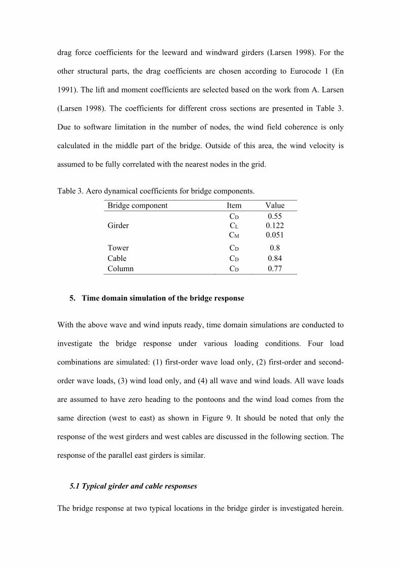
First, the transverse displacement time histories of Node 1 are compared in

Figure 10 (a). It is observed that both the wind and wave loads contribute to the

transverse motion of the bridge girder. However, the wind load results in a much larger

response than the wave load. The transverse displacement has a mean value of around

0.3 m due to the mean wind component. The wave load induced transverse motion has

its mean at 0 m and the maximum displacement is about 0.3 m. The displacement

contributions from different wave and wind loads are also evident from the frequency

plot in Figure 10 (b).

Figure 11 shows the transverse response of Node 2 at the continuous span for

various loading conditions. The wave-induced displacement is in the same range as

Node 1 in the cable-stayed span. However, the wind load results in a significantly larger

transverse motion with a maximum displacement of 2 m. A similar observation can be

found in the frequency domain plot in Figure 11 (b). Again, the wind load has much

larger amplitude and thus dominates the bridge transverse motion in the continuous

zy

x

Cable element

Node 1

Node 2

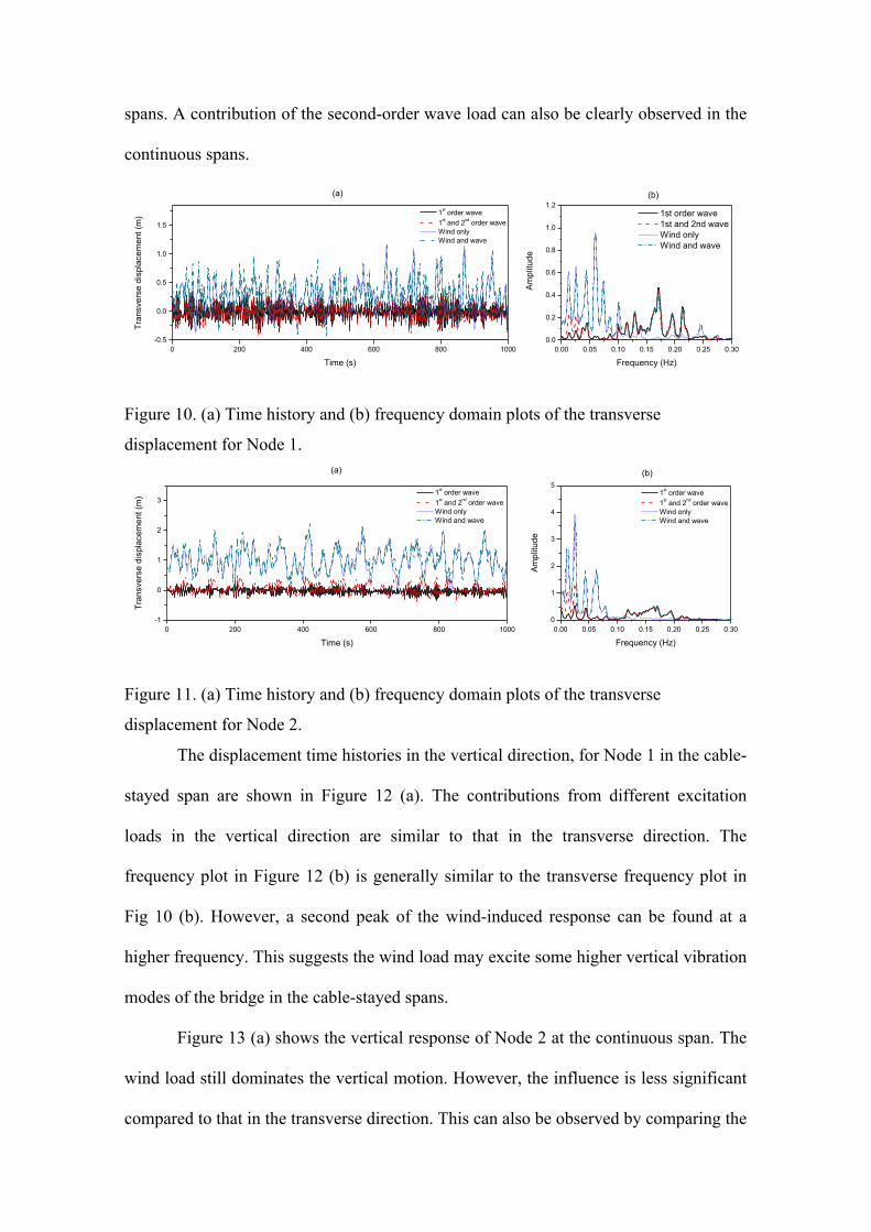
spans. A contribution of the second-order wave load can also be clearly observed in the

continuous spans.

Figure 10. (a) Time history and (b) frequency domain plots of the transverse

displacement for Node 1.

Figure 11. (a) Time history and (b) frequency domain plots of the transverse

displacement for Node 2.

The displacement time histories in the vertical direction, for Node 1 in the cable-

stayed span are shown in Figure 12 (a). The contributions from different excitation

loads in the vertical direction are similar to that in the transverse direction. The

frequency plot in Figure 12 (b) is generally similar to the transverse frequency plot in

Fig 10 (b). However, a second peak of the wind-induced response can be found at a

higher frequency. This suggests the wind load may excite some higher vertical vibration

modes of the bridge in the cable-stayed spans.

Figure 13 (a) shows the vertical response of Node 2 at the continuous span. The

wind load still dominates the vertical motion. However, the influence is less significant

compared to that in the transverse direction. This can also be observed by comparing the

0 200 400 600 800 1000-0.5

0.0

0.5

1.0

1.5

(a)

Tran

sver

se d

ispl

acem

ent (

m)

Time (s)

1st order wave 1st and 2nd order wave Wind only Wind and wave

0.00 0.05 0.10 0.15 0.20 0.25 0.300.0

0.2

0.4

0.6

0.8

1.0

1.2(b)

Ampl

itude

Frequency (Hz)

1st order wave 1st and 2nd wave Wind only Wind and wave

0 200 400 600 800 1000-1

0

1

2

3

(a)

Tran

sver

se d

ispl

acem

ent (

m)

Time (s)


0.00 0.05 0.10 0.15 0.20 0.25 0.300

1

2

3

4

5 1st order wave 1st and 2nd order wave Wind only Wind and wave

(b)

Ampl

itude

Frequency (Hz)

amplitudes in the frequency plots in Figure 13 (b) and Figure 11 (b). The contribution

from the first-order wave load is relatively small and the second-order wave load has

almost no effect on the bridge vertical motion.

Figure 12. (a) Time history and (b) frequency domain plots of the vertical displacement

for Node 1.

Figure 13. (a) Time history and (b) frequency domain plots of the vertical displacement

for Node 2.

The axial force time histories and frequency plots of the selected cable element

are illustrated in Figure 14 (a) and 14 (b), respectively. It can be clearly observed that

the wind load has the greatest influence in the cable axial force while the second-order

wave load has almost no effect. This trend is in line with the girder motion in the cable-

stayed span. The maximum axial force is around 6 MN. With a cross-sectional area of

around 0.0138 m2, this force level only corresponds to an axial stress of 434 MPa. The

stress level corresponds to a utilization level of 23.4% which is much lower than the

acceptable utilization ration of 56%.

0 200 400 600 800 1000-0.10

-0.05

0.00

0.05

0.10

0.15

0.20

0.25(a)

Verti

cal d

ispl

acem

ent (

m)

Time (s)


0.00 0.05 0.10 0.15 0.20 0.25 0.30 0.35 0.400.00

0.05

0.10

0.15

0.20

0.25

0.30(b)

Ampl

itude

Frequency (Hz)

1st order wave 1st and 2nd wave Wind only Wind and wave

0 200 400 600 800 1000-0.4

-0.2

0.0

0.2

0.4

0.6

0.8

(a)

Verti

cal d

ispl

acem

ent (

m)

Time (s)


0.00 0.05 0.10 0.15 0.20 0.25 0.300.0

0.3

0.6

0.9

1.2

1.5 1st order wave 1st and 2nd order wave Wind only Wind and wave

(b)Am

plitu

de

Frequency (Hz)

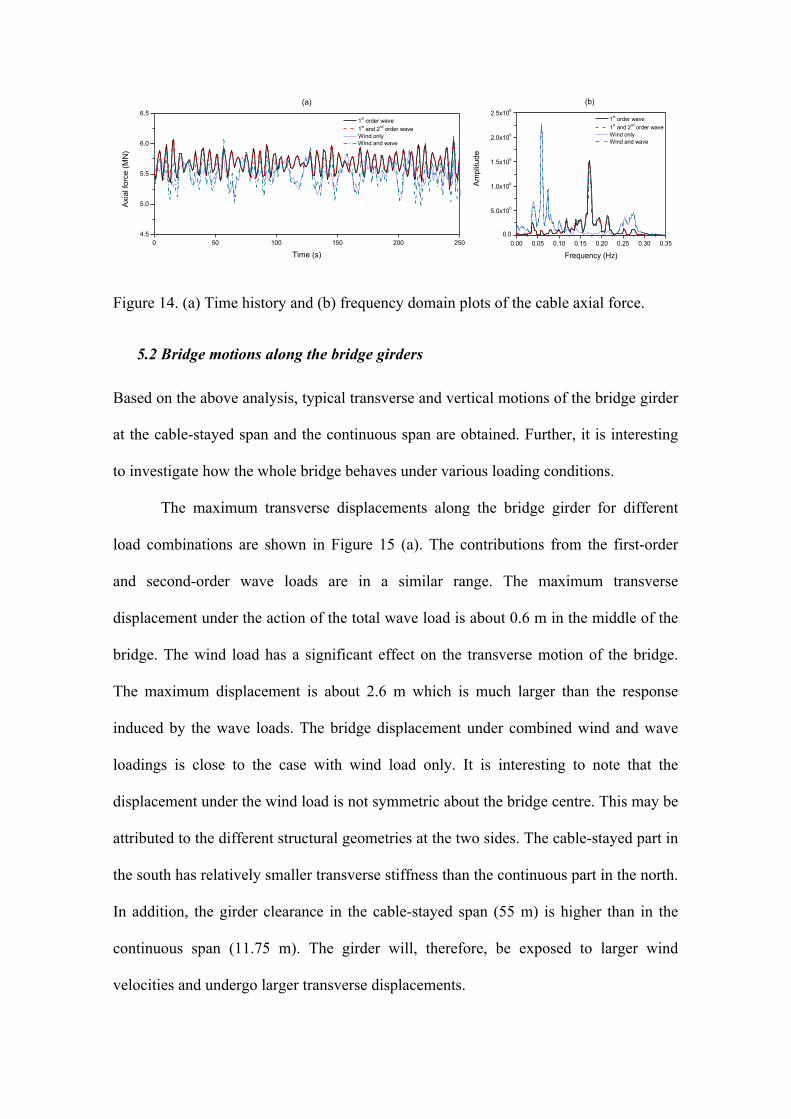
Figure 14. (a) Time history and (b) frequency domain plots of the cable axial force.

5.2 Bridge motions along the bridge girders

Based on the above analysis, typical transverse and vertical motions of the bridge girder

at the cable-stayed span and the continuous span are obtained. Further, it is interesting

to investigate how the whole bridge behaves under various loading conditions.

The maximum transverse displacements along the bridge girder for different

load combinations are shown in Figure 15 (a). The contributions from the first-order

and second-order wave loads are in a similar range. The maximum transverse

displacement under the action of the total wave load is about 0.6 m in the middle of the

bridge. The wind load has a significant effect on the transverse motion of the bridge.

The maximum displacement is about 2.6 m which is much larger than the response

induced by the wave loads. The bridge displacement under combined wind and wave

loadings is close to the case with wind load only. It is interesting to note that the

displacement under the wind load is not symmetric about the bridge centre. This may be

attributed to the different structural geometries at the two sides. The cable-stayed part in

the south has relatively smaller transverse stiffness than the continuous part in the north.

In addition, the girder clearance in the cable-stayed span (55 m) is higher than in the

continuous span (11.75 m). The girder will, therefore, be exposed to larger wind

velocities and undergo larger transverse displacements.

0 50 100 150 200 2504.5

5.0

5.5

6.0

6.5(a)

Axia

l for

ce (M

N)

Time (s)


0.00 0.05 0.10 0.15 0.20 0.25 0.30 0.350.0

5.0x105

1.0x106

1.5x106

2.0x106

2.5x106


(b)

Am

plitu

de

Frequency (Hz)

The vertical displacements of the bridge girder are plotted in Figure 15 (b). As

expected, the second-order wave load has almost no contribution to the vertical motion

of the bridge. The vertical displacement of the bridge girder under the first-order wave

load has a maximum value of 0.25 m. The contribution from the wind load is in a

similar range as that from the wave load. The maximum vertical displacement under the

total environmental load is about 0.5 m.

One of the important considerations in the design of bridges is the maximum

vertical acceleration of the bridge deck. It is required that the vertical acceleration

should not exceed some 0.6 m/s2 (Seif and Inoue 1998) to allow safe traffic and the

comfortableness of the bridge users. As shown in Figure 15 (c), the maximum vertical

acceleration in the continuous part is less than 0.4 m/s2 in all cases. For the cable-stayed

part in the south, the wind-induced vertical acceleration is close to the limit of 0.6 m/s2,

which is considerably larger than that in the continuous spans in the north. This is

because the cable-stayed span is more than twice the length of the continuous span.

Therefore, special design considerations should be exercised to limit the vertical

vibration of the cable-stayed spans. Passive linear and nonlinear dampers have been

widely used to suppress vibration of the stay cables (Main and Jones 2001). Tuned mass

dampers (TMD) and shape memory alloys dampers (SMA) are the most commonly

used damper systems (Cai et al. 2007, Dong et al. 2010). These devices can effectively

reduce cable vibrations. It is found that the cable vibration can be reduced to about 20%

of that without the damping devices (Cai, Wu and Araujo 2007).

Figure 15. (a) Transverse displacement, (b) vertical displacement, and (c) vertical

acceleration of the girder along the bridge.

5.3 Bending and torsional moments along the bridge girders

The bending moment of the bridge girder about the strong axis (z) is plotted in Figure

16 (a). In the cable-stayed spans, the strong axis moment due to the wind load is much

larger than that induced by the wave loads. In the continuous spans, however, the first-

order wave load results in a larger strong axis moment than that induced by the wind

load. This observation matches the transverse displacement distribution in Figure 15 (a).

The displacement increases dramatically from 500 m to 1000 m while it has a much

smaller variation in the middle part of the bridge.

Figure 16 (b) shows the weak axis moment along the bridge girder. The first-

order wave load controls the weak axis bending moment and the second-order wave

0 500 1000 1500 2000 2500 3000 3500 4000 45000.0

0.5

1.0

1.5

2.0

2.5

3.0(a)

Tran

sver

se d

ispl

acem

ent (

m)

Postion (m)


0 500 1000 1500 2000 2500 3000 3500 4000 45000.0

0.1

0.2

0.3

0.4

0.5

0.6

(b)

Verti

cal d

ispl

acem

ent (

m)

Postion (m)


0 500 1000 1500 2000 2500 3000 3500 4000 45000.0

0.1

0.2

0.3

0.4

0.5

0.6

0.7(c)


Verti

cal a

ccel

erat

ion

(m/s

2 )

Postion (m)

load has almost no effect. It is interesting to find that although the wind load results in a

similar magnitude of the vertical motion as the first-order wave load, it has little effect

on the girder weak axis moment. This is because the wind load induced vertical motion

is generally in phase at each pontoon and thus results in a smaller weak axis moment.

The torsional response of the bridge girder is shown in Figure 16 (c). The wind

load dominates the torsional moment in the cable-stayed spans while the first-order

wave load has the most significant effect on the torsional response in the continuous

spans. The wind load also contributes to the torsional moment of the middle part of the

bridge. The second-order wave load has almost no effect on the bridge torsional

response.

0 500 1000 1500 2000 2500 3000 3500 4000 4500-400

-300

-200

-100

0

100

200

300

400(a)

Stro

ng a

xis

mom

ent (

MN

m)

Position (m)

1st order wave 1st and 2nd order wave Wind Wind and wave

0 500 1000 1500 2000 2500 3000 3500 4000 4500-300

-200

-100

0

100

200

300(b)

Wea

k ax

is m

omen

t (M

Nm

)

Position (m)


0 500 1000 1500 2000 2500 3000 3500 4000 4500-300

-200

-100

0

100

200

300

(c)

Tors

iona

l mom

ent (

MN

m)

Position (m)


Figure 16. (a) Strong axis, (b) weak axis and (c) torsional moment of the girder along

the bridge.

5.4 Discussion

The response of the floating bridge responses to various wind and wave load conditions

have been simulated and compared.

The wind load has a large contribution to the bridge motion. It dominates both

the transverse and vertical motions of the bridge girder. The mean wind component

induces a large transverse displacement of more than 2 m. The girder deformation shape

in Figure 15 (a) is similar to the first mode of bridge vibration as shown in Fig 4. This

suggests that the low-frequency wind load may excite some of the horizontal bending

modes of the bridge. The vertical acceleration in the cable-stayed span is large due to

the wind loading. The wind load induces higher bending and torsional moments in the

cable-stayed spans than in the continuous spans.

The first-order wave load contributes also to the bridge motion in the transverse

and vertical directions. The effect is smaller than the wind load as can be observed from

the displacement time histories and frequency plots. However, the first-order wave load

results in larger moments in the bridge girder in all three rotational degrees of freedom.

The second-order wave load influences the transverse motion of the bridge

girders, especially in the continuous spans. However, it has a negligible effect on the

vertical motions of the bridge.

Based on the above discussions, the following recommendations can be given to

improve the current design. In the cable-stayed spans, a vibration-control damper

system as discussed in Section 5.2 may be installed to limit the vertical motion of the

bridge girder and thus ensure a safe traffic. As shown in Figure 16 (c), large weak axis

moments due to the pendulum mode of the pontoons are observed in the cable-stayed

spans. This can be improved by strengthening the girders locally or introducing an

additional connection between the pontoons in axis 3 and 4. For the whole bridge, high

reaction moments occur in the girders at the connection to the supporting column.

Therefore, the girder sections at these locations should also be strengthened locally.

There are several issues which may be of interests for further investigations.

1. No global buckling was observed under the environmental loads in this study.

However, there may be a potential issue regarding the buckling of the bridge in extreme

environmental conditions. Further studies should be conducted to evaluate the global

buckling of the bridge. The accidental limit state design including ship collision loads

should also be carefully checked (Sha and Amdahl 2017).

2. The bridge model is established with beam elements only, it is sufficient to

identify the critical structural members of large plastic utilization. The local behaviour,

plate buckling, for instance, is neglected in the analysis. However, this analysis can be

used as the basis for additional local checks with detailed shell elements at the critical

locations.

3. For the wind and wave data, no measurements have been available when the

current analysis is conducted (COWI 2016). Further investigations should be conducted

when the results from site measurements are available. The analysis in this study only

considers the wind and wave loadings from the west to the east, i.e. zero incidence

angle. A further study can be conducted to investigate environmental loads with

different headings. Bridge responses from short-crested waves can also be of interest in

the future study.

6. Conclusions

In this study, a numerical model of a floating bridge is established. Dynamic time

domain analysis is conducted to investigate the bridge response under environmental

loadings. The first-order and second-order wave loads are calculated by using the

transfer functions obtained from a WADAM analysis based on the linear potential

theory. The dynamic wind load is also included numerically by generating a wind

velocity field in WindSim and applied to the structural model. The bridge responses

under various wind and wave load combinations are investigated.

It is found that the wind load dominates the girder transverse displacement and it

has a large effect on the vertical displacement of the bridge girder. The axial force of the

cable is controlled by the wind load. The axial force level is moderate and well below

utilization limits. The wind-induced vertical acceleration in the cable-stayed spans is

close to the safety limit and a vibration reduction system should be designed and

installed.

Compared with the wind load induced motion, the first-order wave load has a

small effect on the bridge motion in the transverse direction and a comparable

contribution in the vertical direction. The second-order wave load only has a limited

contribution to the transverse bridge displacement.

The first-order wave load has a dominant influence on all bending and torsional

moments of the bridge girder while the second-order wave load has almost no

contribution to the girder response. The wind load induces large bending and torsional

moments in the cable-stayed spans. In addition, it also contributes to the torsional

moment of the girders in the middle bridge.

Acknowledgements

This work was supported by the Norwegian Public Roads Administration (project

number 328002) and in parts by the Research Council of Norway through the Centres of

Excellence funding scheme, project AMOS (project number 223254). These supports

are gratefully acknowledged by the authors.

References

Aas-Jakobsen K. 2015. User manual WindSim. Aas-Jakobsen K, Strømmen E. 1998. Time domain calculations of buffeting response for wind-sensitive structures. Journal of Wind Engineering and Industrial Aerodynamics.74:687-695. Boonyapinyo V, Yamada H, Miyata T. 1994. Wind-induced nonlinear lateral-torsional buckling of cable-stayed bridges. Journal of Structural Engineering.120:486-506. Cai C, Wu W, Araujo M. 2007. Cable vibration control with a TMD-MR damper system: Experimental exploration. Journal of structural engineering.133:629-637. Cao Y, Xiang H, Zhou Y. 2000. Simulation of stochastic wind velocity field on long-span bridges. Journal of Engineering Mechanics.126:1-6. Chakrabarti SK. 1987. Hydrodynamics of offshore structures: WIT press. Chen W-L, Li H, Hu H. 2014. An experimental study on the unsteady vortices and turbulent flow structures around twin-box-girder bridge deck models with different gap ratios. Journal of Wind Engineering and Industrial Aerodynamics.132:27-36. COWI. 2016. NOT-KTEKA-021 Curved bridge - Navigation channel in south. Oslo, Norway. Dong J, Cai C, Okeil AM. 2010. Overview of potential and existing applications of shape memory alloys in bridges. Journal of Bridge Engineering.16:305-315. En B. 1991. 1-4: 2005 Eurocode 1: Actions on structures—General actions—Wind actions. In: NA to BS EN. Faltinsen O. 1993. Sea loads on ships and offshore structures: Cambridge university press. Hasselmann K, Barnett T, Bouws E, Carlson H, Cartwright D, Enke K, Ewing J, Gienapp H, Hasselmann D, Kruseman P. 1973. Measurements of wind-wave growth and swell decay during the Joint North Sea Wave Project (JONSWAP). Hilber HM, Hughes TJ, Taylor RL. 1977. Improved numerical dissipation for time integration algorithms in structural dynamics. Earthquake Engineering & Structural Dynamics.5:283-292. Institution BS. 2004. Eurocode 2: Design of Concrete Structures: Part 1-1: General Rules and Rules for Buildings. In: British Standards Institution. Jia J. 2014. Investigations of a practical wind-induced fatigue calculation based on nonlinear time domain dynamic analysis and a full wind-directional scatter diagram. Ships and Offshore Structures.9:272-296. Kvittem MI, Bachynski EE, Moan T. 2012. Effects of hydrodynamic modelling in fully coupled simulations of a semi-submersible wind turbine. Energy Procedia.24:351-362. Larsen A. 1998. Advances in aeroelastic analyses of suspension and cable-stayed bridges. Journal of Wind Engineering and Industrial Aerodynamics.74:73-90. Livesley RK. 2013. Matrix Methods of Structural Analysis: Elsevier. Main J, Jones N. 2001. Evaluation of viscous dampers for stay-cable vibration mitigation. Journal of Bridge Engineering.6:385-397. Newman JN. Second-order, slowly-varying forces on vessels in irregular waves. Proceedings of the Proc Int Symp Dyn Mar Vehic Struct in Waves, Inst Mech Engrs, London, 1974; 1974. Salvatori L, Borri C. 2007. Frequency-and time-domain methods for the numerical modeling of full-bridge aeroelasticity. Computers & structures.85:675-687. Santos J, Miyata T, Yamada H. Gust response of a long span bridge by the time domain approach. Proceedings of the Proceedings of Third Asia-Pacific Symposium on Wind Engineering, Hong Kong; 1993.

Seif MS, Inoue Y. 1998. Dynamic analysis of floating bridges. Marine structures.11:29-46. Sha Y, Amdahl J. Ship Collision Analysis of a Floating Bridge in Ferry-Free E39 Project. Proceedings of the ASME 2017 36th International Conference on Ocean, Offshore and Arctic Engineering; 2017: American Society of Mechanical Engineers. Søreide TH, Amdahl J, Eberg E, Holmås T, Hellan Ø. 1993. USFOS-A computer program for progressive collapse analysis of steel offshore structures. Theory Manual. SINTEF STF71 F88038 Rev. Veritas DN. 1994. WADAM—Wave Analysis by Diffraction and Morison Theory, SESAM user’s manual, Høvik. Watanabe E, Utsunomiya T, Wang C. 2004. Hydroelastic analysis of pontoon-type VLFS: a literature survey. Engineering structures.26:245-256.

Documents

Numerical investigations of the dynamic response of a