Embed Size (px)
Citation preview

Rochester Institute of Technology Rochester Institute of Technology
RIT Scholar Works RIT Scholar Works
Theses
12-16-2015
Numerical Investigation of Parameters Impacting the Wall Numerical Investigation of Parameters Impacting the Wall
Thickness of Carbon Nanotubes Manufactured by Template-Thickness of Carbon Nanotubes Manufactured by Template-
Based Chemical Vapor Deposition Based Chemical Vapor Deposition
Yashar Seyed Vahedein [email protected]
Follow this and additional works at: https://scholarworks.rit.edu/theses
Recommended Citation Recommended Citation Seyed Vahedein, Yashar, "Numerical Investigation of Parameters Impacting the Wall Thickness of Carbon Nanotubes Manufactured by Template-Based Chemical Vapor Deposition" (2015). Thesis. Rochester Institute of Technology. Accessed from
This Thesis is brought to you for free and open access by RIT Scholar Works. It has been accepted for inclusion in Theses by an authorized administrator of RIT Scholar Works. For more information, please contact [email protected].

R·I·T
Numerical Investigation of Parameters
Impacting the Wall Thickness of Carbon
Nanotubes Manufactured by
Template-Based Chemical Vapor Deposition
By
Yashar Seyed Vahedein
A Thesis Submitted in Partial Fulfillment
of the Requirements for the
Degree of Master of Science in Mechanical Engineering
at
Rochester Institute of Technology
NANO BIO INTERFACE LAB
DEPARTMENT OF MECHANICAL ENGINEERING
KATE GLEASON COLLEGE OF ENGINEERING
ROCHESTER INSTITUTE OF TECHNOLOGY
ROCHESTER, NEW YORK
December 16th, 2015

ii
Numerical Investigation of Parameters
Impacting the Wall Thickness of Carbon
Nanotubes Manufactured by
Template-Based Chemical Vapor Deposition
By
Yashar Seyed Vahedein
A Thesis Submitted in Partial Fulfillment
of the Requirements for the
Degree of Master of Science in Mechanical Engineering
at Rochester Institute of Technology
Approved By:
Prof. _______________________ Dr. Michael G. Schrlau (Thesis Advisor)
Prof. _______________________ Dr. Patricia Taboada-Serrano (Thesis Committee)
Prof. _______________________ Dr. Steven W. Day (Thesis Committee)
Prof. _______________________ Dr. Robert Parody (Thesis Committee)
Prof. _______________________ Dr. Agamemnon Crasidis (Department Representative)
DEPARTMENT OF MECHANICAL ENGINEERING
KATE GLEASON COLLEGE OF ENGINEERING
ROCHESTER INSTITUTE OF TECHNOLOGY
ROCHESTER, NEW YORK
December, 2015

iii
Acknowledgments
I would like to thank my advisor, Professor Michael G. Schrlau, my dear thesis committee
members, Dr. Taboada-Serrano, Dr. Steven Day and Dr. Robert Parody for their valued advice
and support of this work at Rochester Institute of Technology. And my colleagues in NBIL,
especially Ryan Dunn and Masoud Golshadi.
I also want to thank Ms. Brenda Mastrangelo, and Tom Alston for their help in arranging a gas
chromatography session in Rochester Institute of Technology.
My special thanks to my dearest Nargess Hassani and my parents for their support throughout
my MASTERs studies.
iv
Abstract Template-based chemical vapor deposition (TB-CVD) is a versatile technique for
manufacturing carbon nanotubes (CNTs) or CNT-based devices for various applications. In this
process, carbon is deposited by thermal decomposition of a carbon-based precursor gas inside the
nanoscopic cylindrical pores of anodized aluminum oxide (AAO) templates to form CNTs.
Experimental results show CNT formation in templates is controlled by TB-CVD process
parameters, such as time, temperature and flow rate. Optimization of this process is done
empirically, requiring tremendous time and effort. Moreover, there is a need for a more
comprehensive and low cost way to characterize the flow in the furnace in order to understand
how process parameters may affect CNT formation. In this report, we describe the development
of four, three-dimensional numerical models, each varying in complexity, to elucidate the thermo-
fluid behavior inside the TB-CVD process. Using computational fluid dynamic (CFD) commercial
codes, the four models were compared to determine how the presence of the template and boat,
composition of the precursor gas, and consumption of species at the template surface affect the
temperature profiles and velocity fields in the system. The most accurate model will be used to
conduct particle injection/tracking near the templates and to characterize the particle residence
time as a function of time and consumption rate. The developments in this work build the
groundwork for explaining how flow characteristics affect carbon deposition on templates in any
CVD reactor.

v
Acknowledgments ____________________________________________________________________________________ iii
Abstract _________________________________________________________________________________________________ iv
List of Tables __________________________________________________________________________________________ vii
List of Figures ________________________________________________________________________________________ viii
1 Problem Introduction ___________________________________________________________________________ 2
Single cell analysis _____________________________________________________________________________ 2
Carbon nanotubes (CNTs) and their application to single cell analysis _______________ 3
CNT manufacturing and CVD process _______________________________________________________ 4
Empirical and numerical study on TB-CVD ________________________________________________ 6
Conclusion ______________________________________________________________________________________ 8
2 Background ______________________________________________________________________________________ 11
Single-cell analysis tools and CNT-based SCA tools ______________________________________ 11
Carbon nanotubes and their SCA applications ___________________________________________ 12
CNT manufacturing and CVD process ______________________________________________________ 16
Impact of simulation technique on this problem ________________________________________ 20
Experimental setup and numerical simulation of CVD in the tube furnace__________ 21
Reactions _______________________________________________________________________________________________ 22 Solving and verification of thermal-fluidic problems in FLUENT __________________________________ 22
Previous work on CVD process simulation or deposition in porous media _________ 25
Significance of our numerical study _______________________________________________________ 33
3 First Steps towards Model Development ___________________________________________________ 36
Experimental measurements and observations _________________________________________ 36
Developing a numerical model _____________________________________________________________ 37
Model representation of current furnace ____________________________________________________________ 37 Boundary conditions for the problem (general) ____________________________________________________ 38 Solution method and verification ____________________________________________________________________ 39 The need for temperature dependent properties ___________________________________________________ 42 Simplifications applied to the model _________________________________________________________________ 44 Development steps of current numerical simulation _______________________________________________ 45 Mesh independent solution and residuals study ____________________________________________________ 46 Choosing the solver ___________________________________________________________________________________ 48 Further modifications to the model __________________________________________________________________ 49
Model with the sample and boat ____________________________________________________________ 53
Presenting the results as a function of flow rate _________________________________________ 56

vi
Conclusion _____________________________________________________________________________________ 66
4 Model Validation and Development _________________________________________________________ 68
Governing equations and gas properties __________________________________________________ 68
Boundary conditions _________________________________________________________________________ 73
Validation ______________________________________________________________________________________ 76
Modeling Considerations ____________________________________________________________________ 79
Modeling the boat and templates ____________________________________________________________________ 79 Meshing technique ____________________________________________________________________________________ 79
Results and discussion _______________________________________________________________________ 80
Description of model results __________________________________________________________________________ 81 The effect of modeling parameters on thermo-fluid behavior _____________________________________ 88
Conclusion _____________________________________________________________________________________ 95
5 Results and Comparison with Experiment _________________________________________________ 97
Physical system description _________________________________________________________________ 97
Computational methods _____________________________________________________________________ 98 2D transient solution: _________________________________________________________________________________ 99 Particle tracking _____________________________________________________________________________________ 100 Boundary conditions ________________________________________________________________________________ 103 Mesh study ___________________________________________________________________________________________ 104
Results ________________________________________________________________________________________ 105 Reaction ramp up time ______________________________________________________________________________ 105 Experimental trend for total carbon mass deposited as a function of flow rate ________________ 108 Particle tracking to find the residence time of particles __________________________________________ 110 Effect of ethylene consumption rate _______________________________________________________________ 113
Conclusion ___________________________________________________________________________________ 114
6 Conclusion and Future Work _______________________________________________________________ 117
Future work __________________________________________________________________________________ 118
7 References ______________________________________________________________________________________ 119
8 Appendix ________________________________________________________________________________________ 132
Governing equations and two phase model ____________________________________________ 132
Initializing the simulation (Stefen-Maxwell model) ___________________________________ 135
Suggested descriptive statistical analysis _______________________________________________ 136 Suggested statistical approach for analyzing significance in non-repeating data sets _________ 136 Box plots and histograms ___________________________________________________________________________ 143
Particle injection and residence time distribution function. ________________________ 147
vii
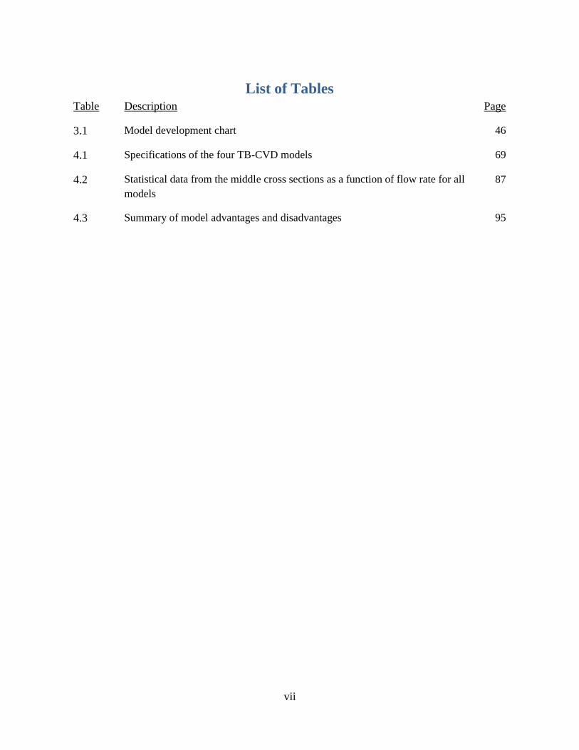
List of Tables Table Description Page
3.1 Model development chart 46
4.1 Specifications of the four TB-CVD models 69
4.2 Statistical data from the middle cross sections as a function of flow rate for all
models
87
4.3 Summary of model advantages and disadvantages 95

viii
List of Figures Title Description Page
1.1 Schematic representations of the TB-CVD system. 6
1.2 Flow chart of the process and the results. 9
2.1 Examples of the developed nanotubes. 14
2.2 Shape and application of nanotubes. 16
2.3 Schematics of CVD model by Spear 1982. 18
2.4 Schematics of a tube furnace and flow conditions inside the furnace, adapted
from (He, Li, and Bai 2011).
21
2.5 Boundary conditions in a vertical CVD reactor adapted from (Ibrahim and
Paolucci 2011).
25
2.6 Schematics (a) and meshed model (b) of vertical reactor for numerical
simulation.
29
2.7 Diagram of the steps required to solve a problem in ANSYS® FLUENT®. 34
3.1 Schematics of Furnace with template and boat positioned inside the tube. 37
3.2 Considering boundary conditions. 38
3.3 2D and 3D model comparison. 2D case and its temperature and velocity
vectors in heated stage of the furnace (a), 3D case and its temperature and
velocity vectors in heated stage of the furnace (b). View of the streamlines
in mid cross section of 3D case (c).
41
3.4 Side and tail views of flow patterns in a converging channel with 8° tilt (Chiu,
Richards, and Jaluria 2000).
43
3.5 Experimental testing of the flow in reactors: visualizing the recirculation using
smoke test in a horizontal reactor (adapted from(Fotiadis and Jensen 1990)) (a),
Gas density profiles visualized using interference holography (Giling 1982)
(b).
44
3.6 Tree chart of model development process. 46

ix
3.7 Meshed tube-furnace model, showing boundary layer meshing for the case
without template (a) modeled geometry of the furnace and 2 meshed models
with and without boat (b).
48
3.8 Comparing the temperature from simulation with experimental data. 50
3.9 Temperature data along the tube over lines that are 1 inch (a) and 2 inches (b)
above the bottom wall of the tube.
52
3.10 Velocity vector plots showing recirculation zones along the tube at 60 sccm (a),
and 200 sccm (b).
53
3.11 Resulted velocity vectors (axial (a), vertical (b), and transverse (c)) around
the samples in cases with and w/out boat.
53
3.12 Mesh independency test – 1.36 M mesh elements is confirmed as a reliable
number of elements.
55
3.13 Contours of temperature for different flow rates on middle cross section of the
tube furnace (a) Statistical analysis of temperature data for 100 sccm (Laminar)
and 200 sccm (Turbulent) (b), box plot summarizing all the data and its trend
(c).
58
3.14 Temperature versus radial position on the cross section in different flow rates. 59
3.15 Contours of axial velocity (also presented as x or u velocity) for different flow
rates on middle cross section of the tube furnace (a), Statistical analysis of u-
velocity data for 100 sccm (Laminar) and 200 sccm (Turbulent) (b), box plot
summarizing all the data and its trend (c).
61
3.16 Contours of vertical velocity (v) for different flow rates on middle cross section
of the tube furnace (a). Statistical analysis of v-velocity data for 100 sccm
(Laminar) and 200 sccm (Turbulent) (b) and box plot summarizing all the data
and its trend (c).
63
3.17 Velocity vectors in the middle cross section of tube furnace, (a) and
streamlines, showing the cross flows (b) and laminar flow (c) vs. turbulent
flow (d), respectively.
64
3.18 Contours of transverse velocity (w) for different flow rates on middle cross
section of the tube furnace.
65
4.1 Schematic representation of the boundary conditions for the TB-CVD tube
furnace.
74
4.2 2D and 3D model comparison. 77
x
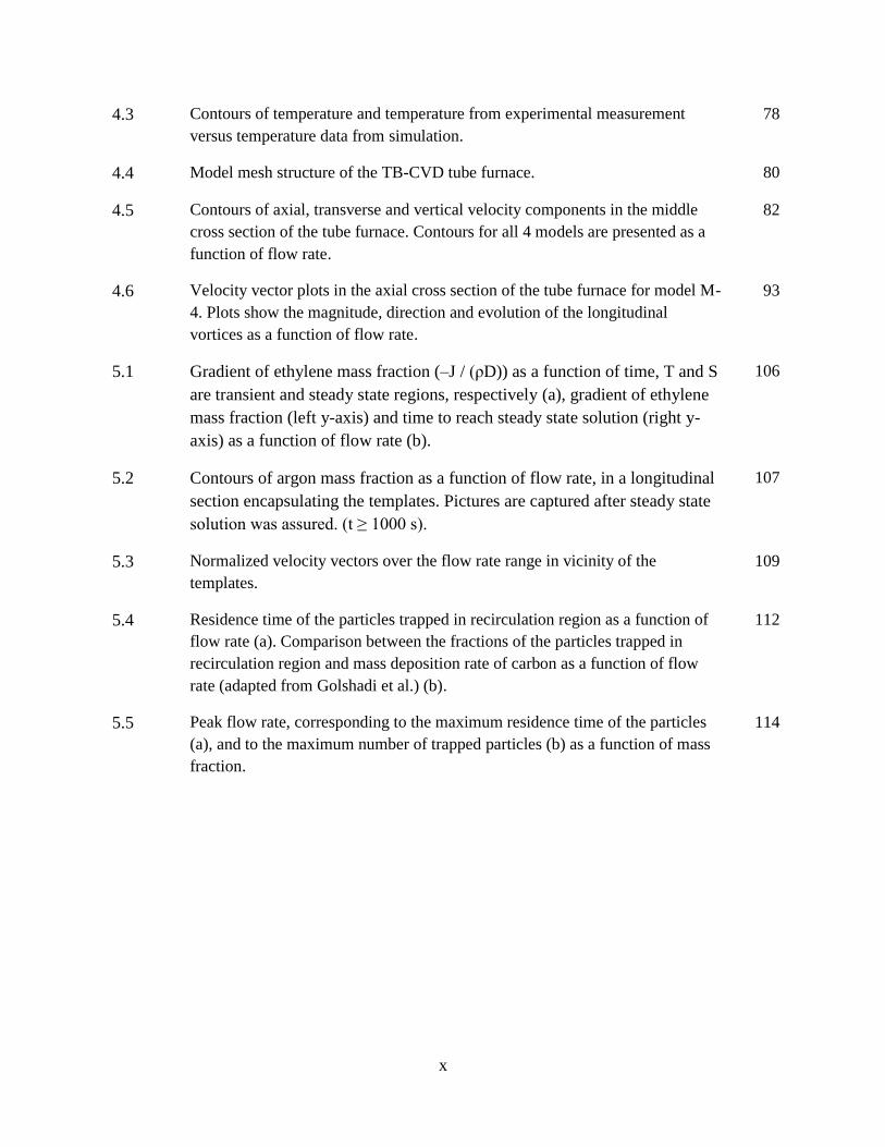
4.3 Contours of temperature and temperature from experimental measurement
versus temperature data from simulation.
78
4.4 Model mesh structure of the TB-CVD tube furnace. 80
4.5 Contours of axial, transverse and vertical velocity components in the middle
cross section of the tube furnace. Contours for all 4 models are presented as a
function of flow rate.
82
4.6 Velocity vector plots in the axial cross section of the tube furnace for model M-
4. Plots show the magnitude, direction and evolution of the longitudinal
vortices as a function of flow rate.
93
5.1 Gradient of ethylene mass fraction (–J / (ρD)) as a function of time, T and S
are transient and steady state regions, respectively (a), gradient of ethylene
mass fraction (left y-axis) and time to reach steady state solution (right y-
axis) as a function of flow rate (b).
106
5.2 Contours of argon mass fraction as a function of flow rate, in a longitudinal
section encapsulating the templates. Pictures are captured after steady state
solution was assured. (t ≥ 1000 s).
107
5.3 Normalized velocity vectors over the flow rate range in vicinity of the
templates.
109
5.4 Residence time of the particles trapped in recirculation region as a function of
flow rate (a). Comparison between the fractions of the particles trapped in
recirculation region and mass deposition rate of carbon as a function of flow
rate (adapted from Golshadi et al.) (b).
112
5.5 Peak flow rate, corresponding to the maximum residence time of the particles
(a), and to the maximum number of trapped particles (b) as a function of mass
fraction.
114

1
Chapter 1

2
1 Problem Introduction
There are wide ranges of applications that require the usage of analytical devices. It can be
utilized in different fields like industry, biomedical studies, electrochemistry, etc. The need for
analytical devices rises from their application in various scientific and industrial applications.
There are areas which need macro-scale devices as the means for analysis but as the scale of
studied systems decrease, smaller tools are required to analyze the system.
Nanotechnology deals with materials and systems at nanometer scales. Subsequently,
nanofabrication is the technique in which designing and manufacturing of nanoscale devices
becomes possible. Nanotechnology has become one of the fastest developing areas in the new
science. Wide range of applications for nanoparticles and nanoscale devices has provided the
means to give nanotechnology the development pace that it currently has. After successful
implementation of microfabrication methods, nanofabrication emerged as the next generation of
fabrication techniques. Since the advent of first transistor in 1974, microelectronics and
semiconductor industries have been the driving force for nanoscale manufacturing. However, by
infusing nanotechnology with another new and fast developing area which was biotechnology, a
new field called nanobiotechnology was born. Nanobiotechnology deals with metabolic
processes of microorganisms. This interdisciplinary combination was the starting point for
creating many innovative tools.
Single cell analysis
All the fundamental life functions of a living organism are being performed by cells. These cells
grow and divide and in the meanwhile they create and/or consume proteins, ions and other
molecules. These functions can be studied and/or controlled (introducing reagents to cells) by the

3
current means of single cell analysis. Single-cell analysis (SCA) has been increasingly
recognized as the key technology for the elucidation of cellular functions, which are not
accessible from bulk measurements on the population level. Various tools and techniques have
been introduced throughout the years since single cell analysis first started to attract significant
attention in science and technology applications. Surface enhanced Raman spectroscopy (SERS)
of active nanoprobes, nanopipette-based patch clamp measurements for analyzing ion channel
activity at subcellular structure – are just two of the examples for the methods being used in
SCA. These examples and more are provided in detail in the literature review, section 2.1.
Carbon nanotubes (CNTs) and their application to single cell analysis
Carbon nanotubes (CNTs) are very prevalent in today’s world of medical research. For instance,
CNTs are being researched in the fields of efficient drug delivery and bio-sensing methods for
disease treatment and health monitoring. Carbon nanotube technology has shown to have the
potential to alter drug delivery and bio sensing methods for the better, and thus, carbon
nanotubes have recently garnered interest in the field of medicine. Because of their high
conductivity, CNT based devices are widely used in electronic devices such as sensors
(Robinson, Snow, and Perkins 2007), field emission devices (J. Li et al. 2004) and hydrogen
storage devices (Ye et al. 1999). In addition to their conductivity, their high strength and
durability makes them an interesting alternative for previous probing devices. Moreover,
exploitation of their unique electrical, optical, thermal, and spectroscopic properties in a
biological context yields great advances in detection, monitoring, and therapy of diseases
(Lacerda et al. 2007) in biomedical institutions and industries.

4
CNT manufacturing and CVD process
Carbon nanotubes have several unique chemical, scale-related, optical, electrical and structural
properties. These properties make them attractive in drug delivery, bio-sensing platforms for the
treatment of various diseases (Bianco, Kostarelos, and Prato 2005), noninvasive monitoring of
blood levels and other chemical properties of the human body, tips for atomic force microscopy
(AFM) and gas sensors (Harris 2009).
Some of the challenges currently apparent in the fabrication of CNTs are as follows:
1. Controlling the orientation of the CNT growth during any process
2. Controlling the Thickness and diameter of the growing tubes
3. Having an integrated structure (defect free) for the CNT
4. Manufacturing CNTs is an expensive process
For more details, the interested reader can refer to the review article by Dai (Dai 2002). The last
two challenges will be automatically lifted when Template-Based CVD (TB-CVD) (Che et al.
1998; Martin 1994; Kyotani, Tsai, and Tomita 1995) is used for manufacturing arrays of CVD.
However, there are some new concerns when using TB-CVD. For example, one of the main
concerns is not knowing the effect of each parameter (such as temperature, flow rate, furnace
dimensions) on the deposited mass of the targeted substance.
Chemical vapor deposition (CVD) is a process suitable for the manufacturing of high-purity,
high-performance solid materials. Compared to other fabrication methods, CVD is more
economical for making CNTs (Choy 2003). In typical CVD, the wafer (substrate) is exposed to
one or more volatile precursors, which reacts/decomposes on the substrate surface to produce the

5
desired deposit. In terms of carbon, Template-Based CVD has the advantage of creating uniform
carbon structure and self-aligned tubes inside the pores of the chosen template.
In order to fabricate CNTs and following the manufacturing success by (Andrews et al. 1999;
Miller, Young, and Martin 2001; Kyotani, Tsai, and Tomita 1995) and similarly carbon
nanopipetts manufactured by (Schrlau et al. 2008) template based manufacturing technique was
used in NBIL1 lab to make uniform CNT structures and template based devices. Schematics of
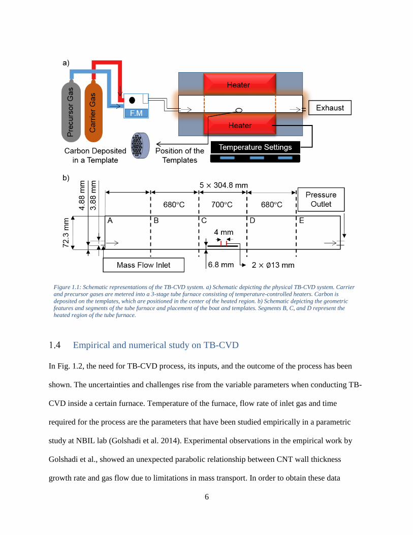
the overall CVD process and critical dimensions and set points of the tube furnace used in TB-
CVD are depicted in Fig. 1.1. As shown in Fig. 1.1a, two gas cylinders containing precursor gas
(30/70 (vol%/vol%) ethylene/helium gas mixture) and carrier gas (argon) are connected to flow
meters for independent control over gas flow into a high temperature, 3-stage tube furnace (max
temperature, 1700°C). The tube of the furnace is 1.524m (5ft) long and has an inner diameter of
72mm (4 inches). Templates are placed vertically in a custom holder inside the tube and
positioned at the center of the heated region - 0.914m (3 ft) of the total tube length - for the
duration of the CVD process and carbon deposition.
The key furnace dimensions and parameters of the experimental CVD process being modeled are
depicted in Fig. 1.1b. In experiments, room temperature (25°C) inlet precursor gas flow was
metered at 20, 40, 60, 80, 100, 200 and 300 sccm. The gas flowed into the CVD furnace where
there are 5 stages: Two room temperature stages (A and E) and three heated stages B, C, and D.
Stages B and D are at 680°C and stage C is at 700°C.
1 Nano-Bio-Interface-Laboratory
6
Empirical and numerical study on TB-CVD
In Fig. 1.2, the need for TB-CVD process, its inputs, and the outcome of the process has been
shown. The uncertainties and challenges rise from the variable parameters when conducting TB-
CVD inside a certain furnace. Temperature of the furnace, flow rate of inlet gas and time
required for the process are the parameters that have been studied empirically in a parametric
study at NBIL lab (Golshadi et al. 2014). Experimental observations in the empirical work by
Golshadi et al., showed an unexpected parabolic relationship between CNT wall thickness
growth rate and gas flow due to limitations in mass transport. In order to obtain these data
Figure 1.1: Schematic representations of the TB-CVD system. a) Schematic depicting the physical TB-CVD system. Carrier
and precursor gases are metered into a 3-stage tube furnace consisting of temperature-controlled heaters. Carbon is
deposited on the templates, which are positioned in the center of the heated region. b) Schematic depicting the geometric
features and segments of the tube furnace and placement of the boat and templates. Segments B, C, and D represent the
heated region of the tube furnace.

7
extensive amounts of time and resources were required. Moreover, experimental CVD parameter
settings are specific to one particular CVD system and their effect on carbon deposition does not
translate from one physical system to another, necessitating development of specific models for
each TB-CVD system that is being employed to manufacture CNTs. This is a general issue with
TB-CVD and other CVD methods. In other words, if different researchers, or a company
commercializing TB-CVD manufacturing technology, wants to duplicate the results using the
same parameters but on a different system, the outcome may be different. Therefore,
understanding the effect of each parameter is essential to create a generalized procedure that can
be used in any system. Other research groups simulated their CVD process to be able to explain
the effect of different parameters on the deposition rate of carbon (Endo et al. 2004; Kuwana, Li,
and Saito 2006) 2. However, there are no simulations or theoretical correlations that can explain
the relation between the success in TB-CVD and the variable parameters of the process.
In this study, we first hypothesized the mass transport limitations, observed in our experimental
work, would be observable as changes in the velocity field around the templates as a function of
flow rate. In Chapters 3 and 4, 2D and 3D macro-scale models were created and compared to
represent the physical system. Four different types of 3D macro-scale models were created to
represent the physical system and determine the effect on process conditions of thermo-fluid
behavior within the reactor. In particular, the results from the four models were compared to
determine how the presence of the boat and templates, composition of the precursor gas, and
consumption of species at the template surface affect the temperature profiles and velocity fields
2 Refer to literature review section for more detail
8
in the system. The benefits and shortcomings of each model, as well as a comparison of model
accuracy and computational time, are presented.
In Chapter 5, the carbon mass deposition ramp up time will be explained using a 2D transient
model of the furnace and finally the results of a 3D steady state model will be presented as the
most accurate model. This model can predict the residence times of the reacting particles without
modeling the individual reactions that are taking place inside the tubular furnace. Therefore, this
simplified model will be validated and used to explain the cause of the experimental observations
for total carbon mass deposited as a function of flow rate as observed in (Golshadi et al. 2014).
The developments in this work build the groundwork for studying how flow characteristics affect
carbon deposition on templates in order to predict the carbon mass deposition in any TB-CVD
reactor.
Conclusion
This work is a step toward predicting the carbon mass deposition trend seen in our experimental
studies and providing a means of predicting how TB-CVD parameters affect the properties of
carbon nanostructures. Figure 1.2 also emphasizes on the fact that, numerical investigation can
optimize the currently established process for manufacturing CNTs in NBIL. By utilizing the
proposed simplified method in this study, accurate prediction of carbon mass deposited during
template based CVD in any TB-CVD furnace setup will be possible.

9
Figure 1.2: Flow chart of the process and the results

10
Chapter 2

11
2 Background
Single-cell analysis tools and CNT-based SCA tools
Cells play a significant role in life activities such as metabolism, signal transduction and so on.
Highly efficient and sensitive detection of the components in single-cell can help to explain
important physiological processes. These means of detection can also throw light on study and
development currently being pursued in the field of biochemistry, cell biology, neurobiology,
medicine, pathology, clinic, etc. (Todd and Margolin 2002). Because of the ultra-small size of
single-cell (diameter 7–200𝜇m, volume fL–nL); ultratrace amount of component (zmol–fmol),
ultra-rapid biochemical reaction (ms), high sensitivity, high selectivity, high temporal resolution
and ultra-small sampling volumes are necessary for single-cell analysis. In the recent years,
single-cell analysis has gone deep into subcellular (local of cytoplast, cellular membrane,
vesicular) and single molecule level. This is why the development of single-cell analysis has
already become the focus of the frontiers in analytical chemistry (Weihua et al. 2000).
So far, SCA has been achieved by miniaturization of established engineering concepts to match
the dimensions of a single cell. However, SCA requires procedures beyond the classical
approach of upstream processing, fermentation, and downstream processing because the
biological system itself defines the technical demands. To understand cell to cell behavior with
their organelles and their intracellular biochemical effect, SCA can provide much more detailed
information from small groups of cells or even single cells, compared to conventional
approaches, which only provide ensemble-average information of millions of cells together. A
short review of micro/nanofluidic methods for single cell analysis has been presented by (Yun
and Yoon 2005) and (Santra and Tseng 2014). There are various tools and techniques which
have been created since single cell analysis attracted scientific attention to itself. Some of the

12
tools that can be used for single cell analysis are listed below (some methods of single-cell
analysis use a combination of these tools (Shi et al. 2010)):
1. Near-field scanning optical microscopy (NSOM)(Betzig et al. 1986) for nanoscale
membrane mapping, as an example for this technique electron microscopy (EM)
spatial resolution around 0.1–10 nm, is powerful to unravel structures and distributions
of various nanometric cellular organelles such as vesicles, lipid rafts etc. The main
limitation of EM is that it only allows static, snapshot observations of fixed cells, and
thus cannot be extended to live cell imaging.
2. Surface enhanced Raman spectroscopy (SERS) active nanoprobes (Fleischmann,
Hendra, and McQuillan 1974).
3. Nanowire-based field effect transistors (FETs) for cellular electrophysiology (Patolsky,
Zheng, and Lieber 2006).
4. Nanopipette-based patch clamp measurements for analyzing ion channel activity at
subcellular structure (Patolsky, Zheng, and Lieber 2006).
For more techniques and tools of conducting single-cell analysis interested reader is referred to
review paper by (Zheng and Li 2012).
Carbon nanotubes and their SCA applications
Ongoing interest in CNTs as components of biosensors and medical devices rose by the
dimensional and chemical compatibilities of CNTs with biomolecules, such as DNA and
proteins. In addition they enable fluorescent (Barone et al. 2005) and photo-acoustic imaging (De
la Zerda et al. 2008), as well as localized heating with the use of near-infrared radiation (Kam et
13
al. 2005)3. But what makes carbon nanotubes so favorable among all the different branches of
chemistry, electrochemistry, nanobiaotechnology and other fields that are stated in (Baughman et
al. 2002), is their outstanding properties. The excitement for carbon nanotubes was first started
when Iijima manufactured highly perfect multiwall tubes as a minor byproduct of fullerene
synthesis using, arc-evaporation (Iijima 1991). Since then and after he made the observation of
single-walled carbon nanotubes (SWCNTs) (Iijima and Ichihashi 1993), CNTs attracted an
exponentially growing attention from research groups all over the world.
Carbon nanotubes (CNTs) are cylindrical shells made, in concept, by rolling graphene sheets into
a seamless cylinder. There exist different types of carbon nanotubes, and even some forms have
an amorphous4 structure. Single wall nanotubes (SWNTs) consist of a single graphene sheet.
This sheet is a planar array of benzene molecules, involving only hexagonal rings with double
and single carbon-carbon bonding. In these tubes the choice of rolling axis relative to the
hexagonal network of the graphene sheet and the radius of the closing cylinder allows for
different types of SWNTs, which vary from insulating to conducting. SWCNTs can interface
with cells at higher spatial resolution because the diameter of a SWCNT is only around 1 nm,
comparable to the size of single protein (Zheng and Li 2012). Multi wall carbon nanotubes
(MWNCTs) are concentrically nested arrays of SWCNTs. MWCNTs were synthesized and
observed a few decades ago –
(L. V.Radushkevich, V. M. Lukyanovich 1952; Oberlin, Endo, and Koyama 1976). Bent, waved,
helically coiled, branched and beaded nanotubes are other forms that have been fabricated
3 For more on this topic interested reader is referred to (De Volder et al. 2013) 4 (Riley 1947) gives a thorough explanation about the differences between the amorphous structure and graphite
structure of carbon.

14
throughout the development of nanotubes(Zhang and Li 2009). These examples are shown in
Fig. 2.1.
Other types of CNTs which have attracted a lot of attention recently, are amorphous CNTs. For
instance, Schrlau et al. developed a process for manufacturing carbon nanopipettes (CNPs)
(Schrlau et al. 2008) by using a CVD process at 900˚C, with argon as a carrier gas and methane
as a precursor gas at flow rates of 200 and 300 sccm, respectively. The thickness of deposited
carbon was controlled by the deposition time (~30 nm at 2 h, ~80 nm at 4 h). It was shown that
CNPs could probe cells in a minimally invasive manner. This ability of CNPs, together with their
hollow and conductive nature, allows for their application in intracellular electrochemistry, drug
Figure 2.1: Examples of the developed nanotubes. Single wall nanotubes: armchair (a), zigzag (b), and chiral (c). Multi
wall nanotubes: Bent (f), branched (g), helical (h). TEM image of MWNT (d) and (e)(Adapted from (Zhang and Li
2009))

15
delivery and fluid injection. This process is still in progress at NBIL. Another popular CVD-
based fabrication technique is template-based manufacturing in which CNTs are formed by
depositing carbon on a template via thermal decomposition of a carbon-carrying precursor gas
(Martin 1994; Kyotani, Tsai, and Tomita 1995). This method is currently being used in NBIL lab
to manufacture CNT embedded devices to use in probing and injection of living cells.
One key advantage of carbon nanotubes is their ability to translocate through plasma membranes,
allowing their use for the delivery of therapeutically active molecules in a manner that resembles
cell-penetrating peptides. The most important parameter in all such studies is the type of carbon
nanotubes used, which is determined by: (i) the preparation and manufacturing process followed;
(ii) the structural characteristics of the CNTs; and (iii) the surface characteristics of the CNTs
and the characteristics of the functional groups at the surface of CNTs (Lacerda et al. 2007).
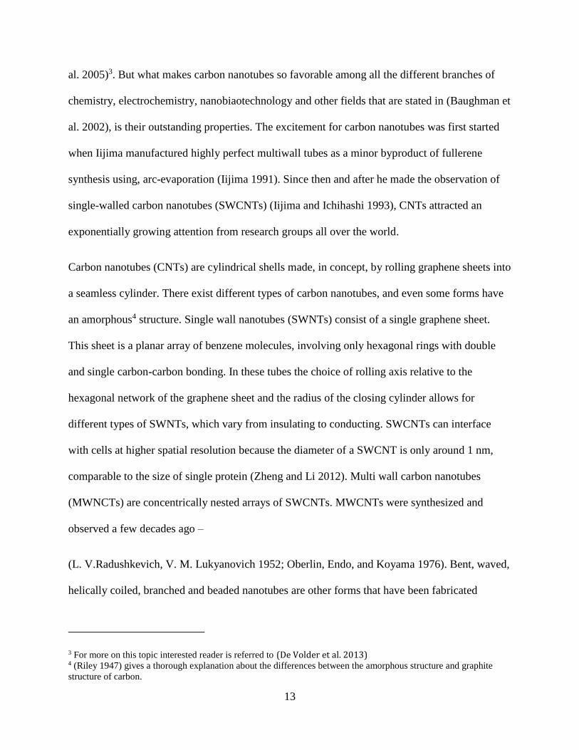
Some of the examples of the CNT or CNP applications are; Singhal et al., which made a CNT-
based endoscope by placing a CNT at the tip of a glass pipette, using a flow through technique
(Singhal et al. 2011)(shown in Figure 2.2), and the carbon nanopippets manufactured in NBIL
lab. For other applications of CNTs a paper by (Ong et al. 2010) can be viewed.
16
CNT manufacturing and CVD process
Carbon nanotubes (CNTs) generally can be synthesized by using a few techniques, such as arc
discharge, laser ablation, chemical vapor deposition (J. Li et al. 2004) and others. Arc-discharge
(Iijima 1991) is a method for the synthesis of CNTs where a direct-current arc voltage is applied
across two graphite electrodes immersed in an inert gas such as He. When pure graphite rods are
used, fullerenes are deposited as soot inside the chamber, and multi-walled carbon nanotubes are
deposited on the cathode. When a graphite anode containing a metal catalyst (Fe or Co) is used
with a pure graphite cathode single-walled carbon nanotubes are generated in the form of soot. In
Laser Ablation (Thess et al. 1996), a high power laser is used to vaporize carbon from a graphite
target at high temperature. Both MWNTs and SWNTs can be produced with this technique. In
order to generate SWNTs, metal particles as catalysts must be added to the graphite targets
similar to the arc discharge technique.
The industrial exploitation of CVD could be traced back to a patent by de Lodyguine in 1893
who had deposited W onto carbon lamp filaments through the reduction of 𝑊𝐶𝑙6 by 𝐻2. Around
Figure 2.2: Shape and application of nanotubes. Optical images of probe tips made from Quartz theta capillaries at various
stages of manufacturing: after pulling (a), after CVD (b), and after etching (c) ( Scale bar 10µm). Schematic of the nanotube
endoscope (d); Scanning electron micrograph of as-assembled endoscope with 50nm carbon nanotube tip (e). picture
Adapted from (Singhal et al. 2011b)
a)
b)
c)
Glass pipette
Non-conducting epoxy
Conducting epoxy
Carbon layer
a)
b)
a)
b)
c)
d)
e)
10

17
that period CVD became an economical method for extraction and pyro-metallurgy for the
production of high purity refractory metals such as Ti, Ni, Zr and Ta. However, it is only in the
past 40 years that a considerable in-depth understanding of the process and the increasing
applications of CVD have been made. In the early 1970s, CVD has attained significant success
in the manufacturing of electronic semiconductors and protective coatings for electronic circuits.
Today, coatings, powders and fibers are some of the materials that are being made, using CVD
process. Micro- and nanofabrication processes widely use CVD to deposit materials in various
forms, including: monocrystalline, polycrystalline, amorphous, and epitaxial. These materials
include: silicon, carbon fiber, carbon nanofibers, filaments, carbon nanotubes, SiO2, silicon-
germanium, tungsten, silicon carbide, silicon nitride, silicon oxynitride, titanium nitride, and
various high-conductivity dielectrics. The CVD process is also used to produce synthetic
diamonds. The chemical reactions of precursor species occur both in the gas phase and on the
substrate. Reactions can be promoted or initiated by heat (thermal CVD), higher frequency
radiation such as UV (photo-assisted CVD) or plasma (plasma-enhanced CVD). CVD is a non-
line-of-sight process with good throwing power. Therefore, it can be used to uniformly coat
complex shaped components and deposit films with good conformal coverage. Such a distinctive
feature outweighs the physical vapor deposition (PVD) process. For other similar CVD
techniques the interested reader is referred to the review paper by Choy (Choy 2003). This
technology is now an essential factor in the manufacture of semiconductors and other electronic
components, in the coating of tools, bearings, and other wear resistant parts and in many optical,
optoelectronic and corrosion applications.
18
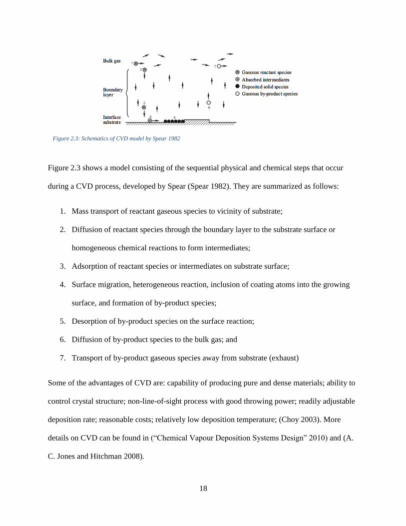
Figure 2.3 shows a model consisting of the sequential physical and chemical steps that occur
during a CVD process, developed by Spear (Spear 1982). They are summarized as follows:
1. Mass transport of reactant gaseous species to vicinity of substrate;
2. Diffusion of reactant species through the boundary layer to the substrate surface or
homogeneous chemical reactions to form intermediates;
3. Adsorption of reactant species or intermediates on substrate surface;
4. Surface migration, heterogeneous reaction, inclusion of coating atoms into the growing
surface, and formation of by-product species;
5. Desorption of by-product species on the surface reaction;
6. Diffusion of by-product species to the bulk gas; and
7. Transport of by-product gaseous species away from substrate (exhaust)
Some of the advantages of CVD are: capability of producing pure and dense materials; ability to
control crystal structure; non-line-of-sight process with good throwing power; readily adjustable
deposition rate; reasonable costs; relatively low deposition temperature; (Choy 2003). More
details on CVD can be found in (“Chemical Vapour Deposition Systems Design” 2010) and (A.
C. Jones and Hitchman 2008).
Figure 2.3: Schematics of CVD model by Spear 1982

19
Template-Based CVD was first used in a naval research laboratory by Martin (Martin 1994), and
Kyotani and coworkers, published the first paper introducing an efficient method for Template-
Based CVD (Kyotani, Tsai, and Tomita 1995). Martin explored the electrochemical method for
deposition of metals inside a micro or nano porous membrane. On the other hand, Kyotani and
coworkers, was able to make the first template based one dimensional carbon nanotube using
CVD process with propylene as the precursor gas. He showed that these tubes can be produced
in an open capped form (encapsulated by other materials), with controllable thickness and
diameter. This process involves synthesizing a certain material inside the micro- and nanopores
of a porous membrane using a low temperature CVD method. Because of the uniform cylindrical
pores with constant diameter inside the commercially available templates, nanostructures with
desired diameter will be synthesized inside these pores. After his first discovery, Martin et al.
continued to explore this newly found method, and published his work on many a number of
different papers (Hulteen and Martin 1997). He tried TB-CVD process with a variety of different
materials (polymers, metals, semiconductors, carbon, etc.) and successfully deposited them
inside the template pores. He was also able to control diameter of carbon nanocylinders (hollow
nanotubes or solid nanofibers). The nanostructures which can be created using this method are
either kept inside the template or can be detached from it to be used separately.
There exists a variety of templates suitable for (TB-CVD). “Track etch” polymeric membranes
(Fleisher, Price, and Walker 1975) and porous alumina membranes (Bockris, John O’M., White,
Ralph E., Conway, Brian E. 2014), are two types of templates that are being used extensively.
Mesoporous zeolites, nanochannel array glass and other materials have also been used and
manufactured as templates (Hulteen and Martin 1997). A comprehensive structural analysis of
template-based CNTs manufactured by CVD in AAO membranes was conducted by (Sarno et al.

20
2012) and (Ciambelli et al. 2011; Ciambelli et al. 2004) to study the degree of crystallinity and
effect of deposition time, temperature, gas mixture and hydrogen feed on CNT synthesis.
Another parametric study has been conducted in NBIL lab to study the effect of inlet gas flow
rate, temperature of furnace and time of the process on CNT synthesis using TB-CVD (Golshadi
et al. 2014). In this work other papers related to the effect of parameters on deposition rate of
carbon are also presented. As it is stated by Choy et al., extensive amounts of time and numerous
experiments are required to study the effect of each parameter on the deposition rate or structure
of the CNTs, formed during TB-CVD (Choy 2003).
Impact of simulation technique on this problem
Simulating a CVD process can be a challenging task since the process has two sides: one is the
advective side of the flow and the other is the convective side of the flow. Since reactions are
also happening, the advective part gets even more complicated when we are trying to model
species conservation and reaction kinetics using a commercially available code for simulating
fluid flows. Similar cases to what is being dealt with in the case of tube furnace in NBIL lab has
been solved previously by using numerical simulation techniques(Yao, Habibian, and O’Melia
1971; Yusong Li 2008; Y. Li et al. 2008). For example Li et al. tried to numerically model
nanoscale fullerene aggregate (nC60) transport and deposition in water-saturated porous media.
A mathematical model that incorporates nonequilibrium attachment kinetics and a maximum
retention capacity was used to simulate experimental nC60 effluent breakthrough curves and
deposition profiles. With some modifications to the classical filtration model, Li et al. was able
to predict the filtration through the nanoporous media and retention of the nanoparticles. One-
dimension convection-dispersion model was also used in the literature to simulate the transport
of MWCNTs in porous media (Dixiao 2012). By looking at the above mentioned papers and a

21
number of others presented in the upcoming literature review, it can be inferred that simulation
can help predict the behavior of the TB-CVD process.
Experimental setup and numerical simulation of CVD in the tube furnace
The schematics of a tube furnace modeled by He et al. is presented in Fig 2.4 (He, Li, and Bai
2011). In this numerical simulation they have tried to capture the carbon synthesis CVD process.
Mass spectrometry was used to identify and quantify the chemical species of the exhaust gas. A
numerical simulation of the reacting gas flow in the reactor was conducted in parallel by taking
into account the space-dependent pyrolysis kinetics of the catalyst and carbon sources, the
reactor temperature gradient and the fluid dynamics. Thereby, they checked the results of
simulation with the concentration readings from mass spectrometry and found out that the data is
in good agreement. Other researchers, who created a 2D transport phenomena model for
chemical vapor deposition, have also tried to create a comprehensive model of their CVD
process (Kleijn 2000).
As stated earlier, the CVD process being used in NBIL lab is thermally activated CVD.
Therefore, reactions and flow conditions are connected to each other. Thermally activated CVD
can be explained by the reactions that are happening and the conditions inside the furnace for any
Figure 2.4: Schematics of a tube furnace and flow conditions inside the furnace, adapted from (He, Li, and Bai 2011)

22
substance being used in the process (Fogler 1986). In order to check the results of any simulation
related to this process running experiments with the same setup and conditions in simulation is
required. In the NBIL lab, this experimental setup is already working and data for thickness of
deposited carbon as a function of each variable parameter already exists.
Reactions
Since FLUENT is being used to conduct Computational Fluid Dynamic (CFD) model of the
CVD process in NBIL lab, it is known that fluent has an embedded reaction and species transport
module. This module can solve reactions in the equilibrium state. In order to solve forced
reaction and coupled diffusion-reaction systems, like the CVD furnace in NBIL lab, it is
necessary to create a reaction diffusion model. Similar works have been done in many different
applications and projects. For instance, Ibrahim and Paolucci used simulation of a vertical CVD
reactor to manufacture aircraft brakes (Ibrahim and Paolucci 2011). This simulation accounted
for a homogeneous gas reaction mechanism as well as a heterogeneous surface reaction
mechanism that is coupled with hydrogen inhibition effect and a pore model. Non-Boussinesq
(low Mach number) equations are used to predict fluid flow, heat transfer, and species
concentrations inside the reactor and within the porous brakes. Results showing the flow,
temperature and concentration fields, as well as the deposition rate of the pyrolytic carbon were
presented. On the other hand, Coltrin, Kee and Miller, presented another useful model that
couples diffusion-reaction system and bulk flow mechanics (Coltrin, Kee, and Miller 1986).
Solving and verification of thermal-fluidic problems in FLUENT
The following are general governing equations in any fluid flow or Navier-Stokes equations:
continuity (Equation 2.1 when phi value is 1), species conservation (Equation 2.2), momentum
conservation (Equation 2.3) and energy conservation (Equation 2.5).

23
∂
∂t∫ ρφdV
V+ ∫ ρφV⃗⃗ ∙dA
A= ∮ Γ∇φ∙dA
A+ ∮ SφdV
V (2.1)
In this equation, ρ is density, V is volume, and A is area. The two terms on the right exist when
diffusion and/or generation due to reaction exists.
∂c
∂t=∇∙(D∇c)-∇∙(v c)+R (2.2)
C is the concentration; D is diffusion constant and R is reaction rate.
𝜌∂
∂t(v̅i)=
∂p
∂xi+ρ
ig
i̅+
∂
∂xi [2μeij-
2
3μ(∇∙V)δij] (2.3)
Where, eij is the strain rate tensor:
eij=1
2(
∂Vi
∂xi+
∂uj
∂xi) (2.4)
And energy equation is:
∂
∂t∫ ρ (e+
1
2v̅2) dV =- ∮ ρ (e+
1
2v̅2) v̅∙dA + ∫ v̅∙fdV
V+ ∮(v̅τ ̅)dA - ∮ qdA (2.5)
Fluent solves all these equations, based on if they are enabled or not, for all mesh elements in a
control volume and iterates until the requested residuals are satisfied.
, Other than having valid experimental data (such as study of mesh dependency, Mesh technique,
residuals, and different solvers.), Versteeg et al. presents the critical preliminary steps to gain
confidence in the simulation (H. K. (Henk Kaarle) Versteeg). Visualization tools can be used to
qualitatively verify the solution. For example these tools can be demonstrated as questions: What
is the overall flow pattern? Is there separation? Where do shocks, shear layers, etc. form? Are
key flow features being resolved? On the other hand, numerical reporting tools can be used to
24
calculate quantitative results: Forces and moments, average heat transfer coefficients, surface
and volume integrated quantities and flux balances are some of the examples. Examining results
to ensure property conservation and correct physical behavior is also required because some high
residuals may be the outcome of having only a few skewed mesh elements. For a given problem,
these are the general steps that will be taken most of the time:
Selecting appropriate physical models; Turbulence, combustion, multiphase, etc.
Define material properties; Fluid, solid, mixture
Prescribe operating conditions.
Prescribe boundary conditions at all boundary zones.
Provide an initial solution.
Set up solver controls.
Set up convergence monitors.
The discretized conservation equations are solved iteratively. A number of iterations are usually
required to reach a converged solution. Convergence is reached when: Overall property
conservation is achieved and changes in solution variables from one iteration to the next are
negligible. Residuals provide a mechanism to help monitor this trend. The accuracy of a
converged solution is dependent upon: Appropriateness and accuracy of physical models, grid
resolution and independence and problem setup.
In the end, to have the completely reliable result, we need to compare the output of fluent with an
experimental setup to get a feel of the reliability and accuracy of the model.
25
Previous work on CVD process simulation or deposition in porous media
Many journal articles report the simulation results for their SWCNT or MWCNT synthesizing
CVD process and a smaller number of them are presenting TB-CVD processes. For simulation of
TB-CVD processes using a precursor gas without catalyst, there exists little or no specifically
important work that can be found in the literature. However, by studying similar works,
analogies were found to help develop a simulation process for our CNT manufacturing
technique. Thereby, some of the similar works has been presented in different parts of this
section. Parts 1, 2 and 3 are the works of (Endo et al. 2004), (Kuwana and Saito 2005) and
(Kuwana, Li, and Saito 2006), respectively. They are modeling CVD reactors in the continuum
regime by considering the chemical reactions in their model. Section 4 shows the work of Mishra
and Verma (Mishra and Verma 2012), who modeled a vertical CVD reactor using a 2D
simulation following the work of (Kuwana and Saito 2005; Cheng, Li, and Huang 2008; Xiao
et al. 2010). In Section 5, it is shown that
He, Li and Bai (He, Li, and Bai 2011)
tried to further improve the work done by
other researchers (section 1-3), by
conducting numerical and experimental
study at the same time. Section 6 presents
the research done by Ibrahim and Paolucci
(Ibrahim and Paolucci 2011), who
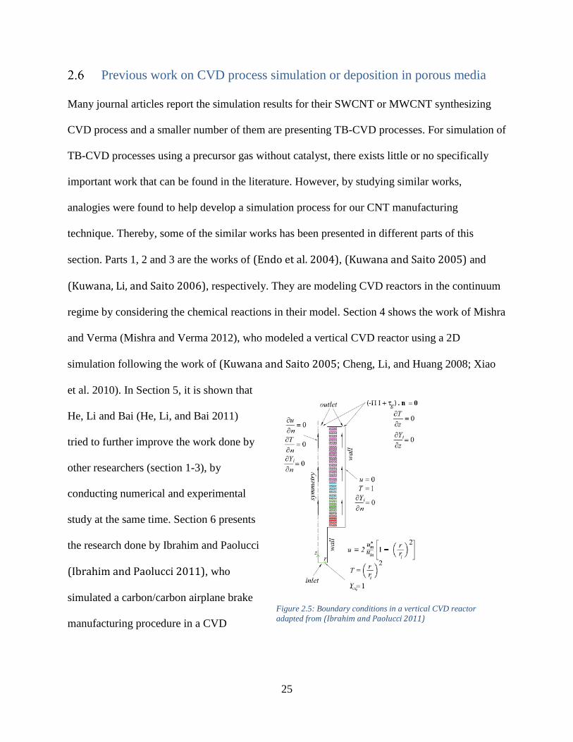
simulated a carbon/carbon airplane brake
manufacturing procedure in a CVD
Figure 2.5: Boundary conditions in a vertical CVD reactor
adapted from (Ibrahim and Paolucci 2011)
26
reactor. This work, gives a new insight on a transient reaction rate-based method of modeling
deposition inside porous media.
1. CFD prediction of carbon nanotube production rate in a CVD reactor
Endo et al. tried to predict carbon nanotube production rate in their CVD reactor (Endo et al.
2004). The reactions in their experimental setup starts with iron catalyst deposition due to
ferrocene decomposition. Then xylene is supplied to the carrier gas (argon with 10% hydrogen).
The xylene and the carrier gas are pre-heated to maintain a laminar flow. For the fluid dynamics
model, they used a 3D laminar, steady state flow with both gas phase and surface chemical
reactions. Using temperature dependent properties of species and properties of the gas mixture
calculated based on the mixing law, the conservation of mass, momentum, energy and species
were solved for an ideal gas. They successfully predicted uniform velocity and temperature
distributions inside the furnace. By coupling the results with reactions, they calculated the
concentration and got a 90% agreement of their data with experimental results. Shape of the flow
in this study showed that buoyancy effects are negligible, justifying the use of a 2D-
axisymmetric model. They used the characteristics of the flow inside the furnace with a simple
CFD model and coupled it with the equations for the deposition reactions, which can be
enhanced using a detailed CFD model that can predict the fluid dynamics inside and between the
templates.
2. Modeling CVD synthesis of carbon nanotubes: Nanoparticle formation from ferrocene
In their study, Kuwana and Seito created a CFD model of the furnace setup based on the work
previousely introduced in the literature (Andrews et al. 1999). This model can predict the
synthesis of multi-walled carbon nanotubes using xylene as a carbon source and ferrocene as a

27
catalyst precursor (Kuwana and Saito 2005). Detailed literature review on the methods to
model reaction mechanisms is presented in their work, and since it can be easily coupled with
CFD simulation, the simplified model by (Kruis et al 1993) has been used to simulate the
formation of iron nanoparticles from ferrocene. Time-dependent Equations 2.6 and 2.7, were
solved together with species conservation equations at a furnace temperature of 973 K. A time
step of 1 ms was used and a steady state was achieved at a flow time of about 200 s. It was
assumed that all particles that reach the reactor wall attach to the wall, that is, Vp (volume
fraction of particle) = Np = 0 at walls. The surface growth of particles deposited on the walls was
not considered. To simulate ferrocene decomposition a one-step chemical reaction was
implemented.
∂Np
∂t+∇.(uNp)=∇.(Dp∇Np)-
1
2βNp
2+I (2.6)
∂Vp
∂t+∇.(uVp)=∇.(Dp∇Vp)-voI+Np (2.7)
They showed the distribution of temperature, ferrocene mole fraction, the rate of ferrocene
reduction due to gas-phase reaction, and the rate of ferrocene reduction due to reaction at the
surface of Fe particles near the entrance to the furnace, all at the steady state. They found out that
the flow field affects the rate of ferrocene reduction as well as the temperature and concentration
fields near the entrance to the furnace. They also showed that there is an increase in particle
diameter (dp) with an increase in the axial distance, achieving the maximum diameter of about
100 nm near the reactor exit, and also a larger particle diameter near the wall as compared to at
the center of the reactor. Temperature dependency of the nucleation also studied and the results
shows an increase in particle diameter with an increase in temperature.

28
3. Gas-phase reactions during CVD synthesis of carbon nanotubes: Insights via numerical
experiments
Following the work of Endo et al. (Endo et al. 2004), Kuwana, Li and Saito (Kuwana, Li, and
Saito 2006), tried to use a more detailed chemical reaction formulation to mimic the situation in
the larger furnace with higher temperature (1473 K) and higher feed rate of 25 g/min, which was
first developed by Kim et al. (Kim et al 2005). To conduct the simulations, they used a
combination of the xylene reaction model of Gaïl and Dagaut and the soot formation model of
Frenklach and his co-workers. They used a semi-implicit extrapolation method (Press et al.,
1992) to integrate following equations (Ianni, 2003) and to reproduce chemical kinetic data in
good agreement with the experiments.
dCi
dt= ∑ [(vri
'' -vri' ) (kr ∏ Ck
vrk'
k -kr
KC,r
∏ Ck
vrk''
k )] +ωi̇r (2.8)
dMr
dt=Rr+Gr+Wr, r=0, 1, 2,…, 5. (2.9)
They measured soot yield and surface area at different temperatures and xylene concentrations
and compared with experimental results from (Tesner and Shurupov 1994).
4. A CFD study on a vertical chemical vapor deposition reactor for growing carbon
nanofibers
(Mishra and Verma 2012) conducted 2D, CFD simulation on the vertical furnace setup shown on
Fig 2.6. They solved mass and momentum conservation equations, with an added momentum
term in order to calculate the momentum equation5 on porous zones in addition to gaseous
5 Detailed equations have been provided in Chapter 3.1 of (Mishra and Verma 2012)

29
mixture zones. They used temperature dependant properties of the fluid so that the buoyancy
effects and therefore natural convection can also be included in their model. The species
transport equation was used to model the deposition of carbon over the substrate. Meanwhile, to
calculate the energy equation, they modified the thermal conductivity coefficient on the porous
medium to be able to add conduction flux term of porous medium in the energy equation.
Temperatures of at least 1273 K was applied on the furnace wall to maintain the required 1073 K
gas temperature to carry out the decomposition of benzene 𝐶6𝐻6 and grow CNTs.
They calculated the carbon deposition rate which was corresponding to the carbon nanofiber
(CNF) – yield of their active carbon fibers (ACF). Also, they found out that the concentration
and temperature profiles are approximately uniform, and smaller velocity and carbon deposition
exists for the case with asymmetric exit for CVD gas products. They verified the data with
analytical correlations for heat and mass transfer, however, they were not able to experimentally
validate their model
Figure 2.6: Schematics (a) and meshed model (b) of vertical reactor for numerical simulation
30
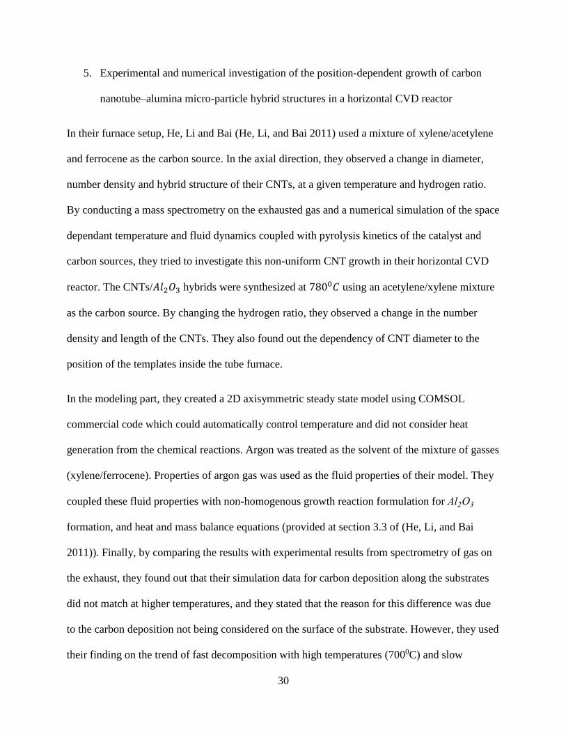
5. Experimental and numerical investigation of the position-dependent growth of carbon
nanotube–alumina micro-particle hybrid structures in a horizontal CVD reactor
In their furnace setup, He, Li and Bai (He, Li, and Bai 2011) used a mixture of xylene/acetylene
and ferrocene as the carbon source. In the axial direction, they observed a change in diameter,
number density and hybrid structure of their CNTs, at a given temperature and hydrogen ratio.
By conducting a mass spectrometry on the exhausted gas and a numerical simulation of the space
dependant temperature and fluid dynamics coupled with pyrolysis kinetics of the catalyst and
carbon sources, they tried to investigate this non-uniform CNT growth in their horizontal CVD
reactor. The CNTs/𝐴𝑙2𝑂3 hybrids were synthesized at 7800𝐶 using an acetylene/xylene mixture
as the carbon source. By changing the hydrogen ratio, they observed a change in the number
density and length of the CNTs. They also found out the dependency of CNT diameter to the
position of the templates inside the tube furnace.
In the modeling part, they created a 2D axisymmetric steady state model using COMSOL
commercial code which could automatically control temperature and did not consider heat
generation from the chemical reactions. Argon was treated as the solvent of the mixture of gasses
(xylene/ferrocene). Properties of argon gas was used as the fluid properties of their model. They
coupled these fluid properties with non-homogenous growth reaction formulation for Al2O3
formation, and heat and mass balance equations (provided at section 3.3 of (He, Li, and Bai
2011)). Finally, by comparing the results with experimental results from spectrometry of gas on
the exhaust, they found out that their simulation data for carbon deposition along the substrates
did not match at higher temperatures, and they stated that the reason for this difference was due
to the carbon deposition not being considered on the surface of the substrate. However, they used
their finding on the trend of fast decomposition with high temperatures (7000C) and slow
31
decomposition on lower temperatures (below 6000C) and suggested the use of acetylene to
increase this rate. They also suggested a new model of gas injection from both sides, based on
their results for fluid dynamics and temperature dependencies of the carbon deposition in their
horizontal tube furnace.
6. Transient solution of chemical vapor infiltration/deposition in a reactor
Ibrahim and Paolucci, worked on simulating a carbon/carbon airplane brake manufacturing
procedure in a vertical CVD reactor (Ibrahim and Paolucci 2011). Species and mass transfer
conservation equations have been solved and dimensionless parameters6 were presented to
represent the diffusion flux, and mass deposition rate in porous medium. A coupled volume of
fraction (VOF) and level set (interface tracking) method was utilized. This method can also be
used when simulating a horizontal reactor and carbon deposition on the porous medium of
templates. To model the mass transfer, a reduced reaction model for carbon CVD/CVI process
by (Birakayala and Evans 2002) is introduced which considers the mass transport with a rate
coefficient for different reactions. This rate can be added to the species and mass transfer
conservation equation to simulate the required reaction.
A road map for a transient simulation has been provided which can also be used for a transient
simulation of horizontal CVD reactor:
I. Integrate reaction source terms7 for the scalar variables (temperature, species mass
fractions and porosity) through a half-time-step (reaction half-step).
6 Froude, Reynolds, Peclet, Darcy, Schmidt, Damkohler numbers and also the dimensionless permeability and
temperature ratios. 7 Kamel (Ibrahim) JK 2007 , Ibrahim J, Paolucci S 2009

32
II. Integrate convective and diffusive terms for the same variables through a full-time-step
by using the solution from the previous step (convection–diffusion full-step).
III. Integrate reaction source terms for the same variables through a half-time-step by using
the solution from the previous step (reaction half-step).
IV. Predict the intermediate velocity field using BDF2 for the pressure-split momentum
equations using solutions from the previous step.
V. Solve the Poisson equation for pressure using the intermediate velocities from the
previous step to obtain the pressure field.
VI. Perform a projection to obtain the velocity field by using the solution of pressure and
intermediate velocities from the previous two steps.
VII. Innovative coupled fluid–structure interaction model for carbon nanotubes conveying
fluid by considering the size effects of nano-flow and nano-structure
In this study (Mirramezani, Mirdamadi, and Ghayour 2013) investigated the effect of viscosity of
a fluid flow in a channel and the interaction between the fluid and structure. Size dependant
continuum theorems and fluid mechanic principles such as Navier-Stokes equations have been
used.
2.10
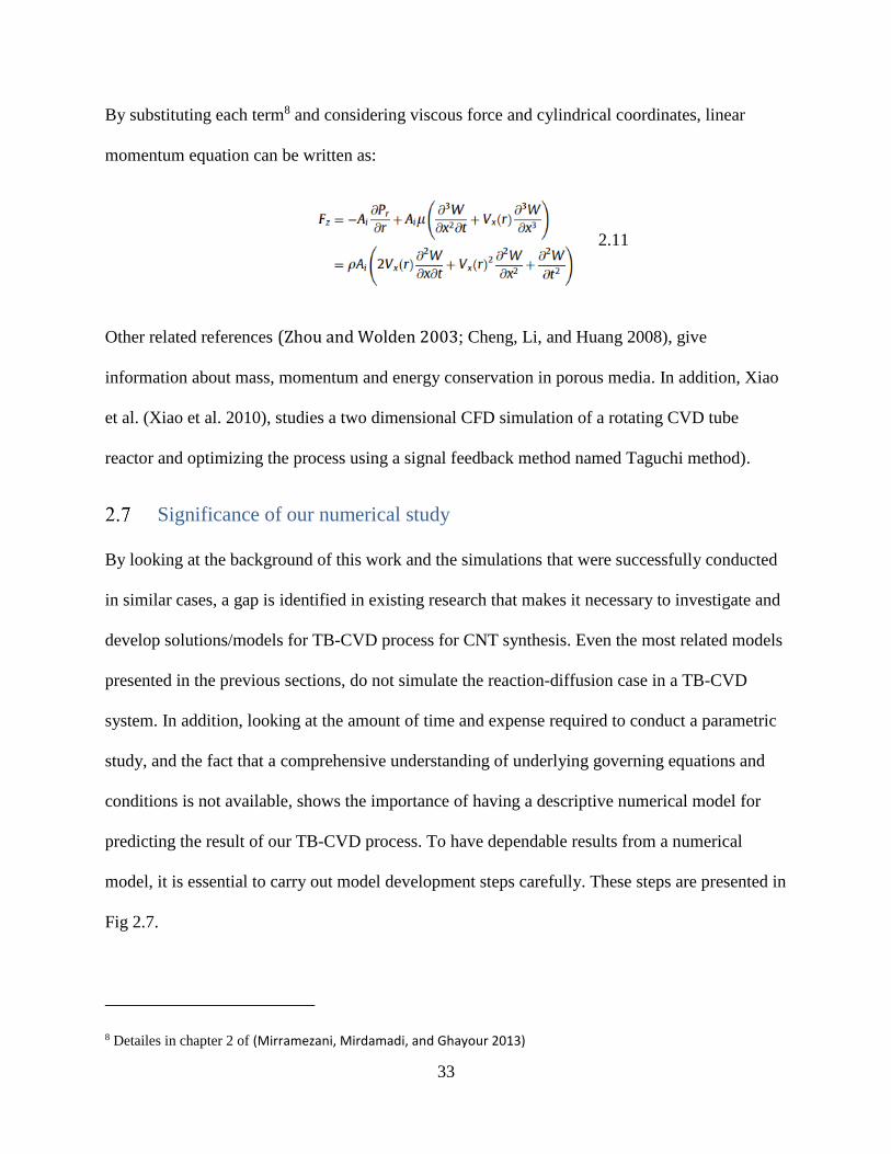
33
By substituting each term8 and considering viscous force and cylindrical coordinates, linear
momentum equation can be written as:
Other related references (Zhou and Wolden 2003; Cheng, Li, and Huang 2008), give
information about mass, momentum and energy conservation in porous media. In addition, Xiao
et al. (Xiao et al. 2010), studies a two dimensional CFD simulation of a rotating CVD tube
reactor and optimizing the process using a signal feedback method named Taguchi method).
Significance of our numerical study
By looking at the background of this work and the simulations that were successfully conducted
in similar cases, a gap is identified in existing research that makes it necessary to investigate and
develop solutions/models for TB-CVD process for CNT synthesis. Even the most related models
presented in the previous sections, do not simulate the reaction-diffusion case in a TB-CVD
system. In addition, looking at the amount of time and expense required to conduct a parametric
study, and the fact that a comprehensive understanding of underlying governing equations and
conditions is not available, shows the importance of having a descriptive numerical model for
predicting the result of our TB-CVD process. To have dependable results from a numerical
model, it is essential to carry out model development steps carefully. These steps are presented in
Fig 2.7.
8 Detailes in chapter 2 of (Mirramezani, Mirdamadi, and Ghayour 2013)
2.11

34
Figure 2.7: Diagram of the steps required to solve a problem in ANSYS® FLUENT®

35
Chapter 3
36
3 First Steps towards Model Development
Experimental measurements and observations
For CNTs manufactured from AAO membranes by template-based CVD using 30 % ethylene
precursor gas, it was found that the deposited mass and wall thickness followed three deposition
regimes with time over the range tested. Nucleation was followed by normal deposition, in which
carbon atoms were deposited layer by layer on the AAO surfaces until the pores were covered by
a surface carbon layer. The effect of furnace temperature, gas flow and deposition time on CNT
wall thickness and structural features were studied in an orthogonal manor; in each set of
experiments, one parameter was changed while the others remained unchanged. Orthogonal
experiments were conducted for synthesis temperatures of 675, 700, 750 and 800 °C, gas flow
rates of 20, 40, 60, 80, 100, 200, and 300 sccm and deposition times of 2.5, 5, 7.5, 10, 15 and 20
h, resulting in AAO-embedded CNTs having wall thicknesses between 12 and 87 nm.
For changes in precursor gas flow rate, it was found that deposited mass and CNT wall thickness
both reached a maximum at 100 sccm, where mass transport and reaction kinetics limited
deposition, respectively, below and above this threshold. It was shown that carbon morphology
did not change over the range of the three parameters tested. For changes in reaction temperature
within the range tested, the deposited mass increased nearly linearly, as did CNT wall thickness
up to 750 °C, where it reached a maximum due to a complete carbon coating of the membrane
surface and covering of the membrane pores. At temperatures above this threshold, carbon was
continually deposited on the membrane surfaces resulting in a thick carbon film connecting the
ends of the AAO-embedded CNTs.

37
Temperature data around the samples are measured using a thermocouple sampling method in
the known flow rate of 500 sccm and 0 sccm on the positions shown in Fig. 3.7. These
temperatures have been compared with the first iterations of numerical model (details in can be
found in Golshadi et al. 2014).
Developing a numerical model
Model representation of current furnace
Schematics of the furnace have been shown in Fig. 3.1. As it can be seen from the figure, inlet
flow rate ranges from 20 to 100 sccm, by increments of 20 sccm, and it also covers 200 sccm and
300 sccm. Temperature of this inlet gas is room temperature (250C). There are 5 stages in the
furnace from which three of them are heated stages and the outsides of stages A & E are subject
to air. Stages B and D are at 6800C and C is at 7000C. Dimensions of the tube are provided in the
figure. During the first efforts to model the furnace, template and boat (sample holder) were not
modeled. They were added after finding a solution which could describe the flow structure inside
the tube furnace (Section 3.3).
Figure 3.1: Schematics of furnace with template and boat positioned inside the tube

38
Boundary conditions for the problem (general)
Figure 3.2 shows the boundary conditions used for developing the numerical mode. Two stages
are considered to be adiabatically isolated, these two are A and E. So they act in such a way that
a perfect isolator would act and do not transmit any heat to the surrounding air. Stages B, C and
D are isothermal walls. In other words, they are thermally connected by a thermally conductive
boundary to a constant-temperature reservoir and their temperature will remain constant. In case
of the NBIL furnace stages B and D are at 6800Cand C is at 7000C as the constant wall
temperature. The inlet boundary is defined as a mass flow inlet boundary condition perpendicular
to the area of the inlet. Therefore, Reynolds number of the inlet flow can be calculated for each
flow rate separately to check if the flow is turbulent or laminar.
Figure 3.2: Considering boundary conditions
Heated Walls
Mass Flow Inlet = Static pressure
D=3.88 mm and 4.88 mm above the bottom wall

39
Due to the sudden expansion after the inlet of the tube, it is possible that flows with 200 and 300
sccm flow rates are turbulent (Koronaki et al. 2001). Therefore, in this section turbulent model
was solved for 200 and 300 sccm (in future sections this model will not be used anymore). The
outlet boundary condition has been set to zero pressure outlet. Therefore, static pressure is zero.
Following equation shows the calculation method of the outlet boundary pressure, thereby, flow
will always move towards outside with the current simplification of exit pressure = 0.
𝑝𝑓 = 0.5(𝑝𝑐 + 𝑝𝑒) + 𝑑𝑝 (3.1)
𝑝𝑐 is the interior cell pressure at neighboring cell to the exit, 𝑝𝑒is the specified exit pressure, and
dp is the difference between specified pressure and the latest average pressure for the boundary.
This value is defined as follows:
𝑑𝑝 = (𝑝𝑒 −∑ 0.5(𝑝𝑐+𝑝𝑒)(𝑎𝑟𝑒𝑎)
𝑖=𝑛𝑓𝑎𝑐𝑒𝑖=1
∑ 𝐴𝑟𝑒𝑎𝑖=𝑛𝑓𝑎𝑐𝑒𝑖=1
) (3.2)
Solution method and verification
First a 2D model of the furnace was simulated which can be viewed in Fig 3.3a. In this 2D
model, all boundary conditions were matched with the 3D physical tube. However, as it can be
viewed in Fig. 3.3c, due to the combined conduction and convection between the heated wall and
the ethylene gas inside the tube, a circular flow exists in the tube furnace. This disturbance is
perpendicular to the direction of flow and mostly resembles the 3D Benard convection
phenomena. In the 2D model, this circular flow cannot be captured. On the other hand, the
position of the inlet and outlet (refer to Fig. 3.1), prevents us from creating an axisymmetric
model. In addition, another problem in 2D model is that it fails to simulate temperatures around
the template as accurate as a 3D model. This is caused by the fact that the cross flows are being

40
neglected in 2D case. These cross flows are an essential phenomenon in tube furnaces and their
shape matches with experimental observations (Fotiadis and Jensen 1990).
In Section 3.4, it will be shown that maximum temperature is no longer 973 K. This modification
has been made after the data for temperature was compared with experimental measurements. It
was found that the maximum temperature inside the tube furnace is lower than the specified
temperature setpoint of the furnace.

41
Figure 3.3: 2D and 3D model comparison. 2D case and its temperature and velocity vectors in heated stage of the furnace
(a), 3D case and its temperature and velocity vectors in heated stage of the furnace (b). View of the streamlines in mid cross
section of 3D case (c).
a)
b)
c)

42
The need for temperature dependent properties
Various combinations of the model have been tried and their advantages were compared. The
first priority was to have a simple model with computationally less expensive solution, therefore,
the method of selection was chosen as follows. During each of the stages in the model
development process, some simplifications were proposed and they have been checked with a
similar numerical model that was less simplified compared to the physical furnace setup. When
comparing to the comprehensive model, if the simplified case could predict the velocity profiles
and temperature with an error percentage of 5% or lower, it would be marked as an acceptable
model and would replace the more complex model for the next iteration of comparisons.
The first type of models developed were laminar steady state flows inside the 3D tube furnace
with constant density, viscosity and thermal conductivity. It was observed that due to the lack of
temperature dependent properties, these models output data similar to a plug flow problem, in
which a fluid flows in a tube with fully developed velocity and temperature profile. Therefore,
these models cannot show the change in density (buoyancy effects). The second type of models
developed were using Boussinesq approximation with a given constant density. The Boussinesq
model should not be used if the temperature differences in the domain are large. In addition, it
cannot be used with species calculations, combustion, or reacting flows. In other words this is a
good approximation for a case which is nearly incompressible. The third type of models. had
temperature dependent properties. Since these models have temperature dependent viscosity and
thermal conductivity, they manage to demonstrate buoyancy and flow shear effects, and thereby
gives the most complete solution. Temperature dependent properties were modeled using piece-
wise linear approximation.

43
A simple analysis of non-dimensional numbers in the third case shows an analogy with the flow
structure from (Chiu, Richards, and Jaluria 2000), shown in Fig. 3.4.
• Since Re < 2300 (laminar) for tube flow, the laminar solver can be used.
• Comparing the Grashof and Reynolds number with flow patterns for a tube flow given in
literature (Chiu, Richards, and Jaluria 2000). We would expect to see something similar
to case (b).
The smoke-trace technique has also been used to demonstrate the existence of buoyancy-driven
recirculations, the so-called transverse roll cells (Van Opdorp and Leys 1987; Visser et al. 1989;
Fotiadis and Jensen 1990), as well as longitudinal roll cells (F. C. Eversteyn 1970) in horizontal
reactors. An example of a recirculating flow is given in Fig. 3.5. Natural-convection-driven
flows and their interactions with the imposed flow field have also been investigated in barrel
reactors (Lord 1987).
Figure 3.4: Side and tail views of flow patterns in a converging channel with 8° tilt (Chiu, Richards, and Jaluria 2000)

44
Simplifications applied to the model
In the case presented in this section, the inlet gas is considered to be ethylene (not a mixture of
helium and ethylene, which is the case in physical system). This decision was made to simplify
the calculation process of heat transfer and fluid flow in the tube. Otherwise, having two gasses
would require a gas mixture, and mixing gas laws would add to the uncertainty of the solution.
This simplification was performed after checking the thermal conductivity and viscosity of
ethylene and helium and noticing that they are both in the same order of magnitude and relatively
close in high temperatures (Holland, Eaton, and Hanley 1983; Bich, Millat, and Vogel 1990;
Poling 2001). Therefore, it can be assumed that they would show similar behavior to the changes
in temperature. On the other hand, compressible flow is modeled using ideal gas formulation for
density variations.
It is also assumed that the Argon which may reside inside the tube at the first minutes of the
process is being flushed out completely when the inlet gas mixture enters the CVD chamber in
NBIL (the tube furnace). Thereby, the amount of time that argon can have any effects on the
process conditions or temperature of the furnace is assumed to be negligible compared to the
a) b)
Figure 3.5: Experimental testing of the flow in reactors a) visualizing the recirculation using smoke test in a
horizontal reactor (adapted from(Fotiadis and Jensen 1990)), b) Gas density profiles visualized using interference
holography (Giling 1982).

45
entire process (Argon will be included in the model presented in Section 5). Another
simplification that is considered here, is that we are neglecting the effect of radiation heat
transfer.
Development steps of current numerical simulation
In total, more than 60 different numerical simulations were tried to achieve the final model
presented for the macro-scale representation of the bulk flow in NBIL tube furnace setup. Table
3.1 and Fig. 3.2 are showing the entire development trend of CFD model.
Table 3.1: Model development chart.
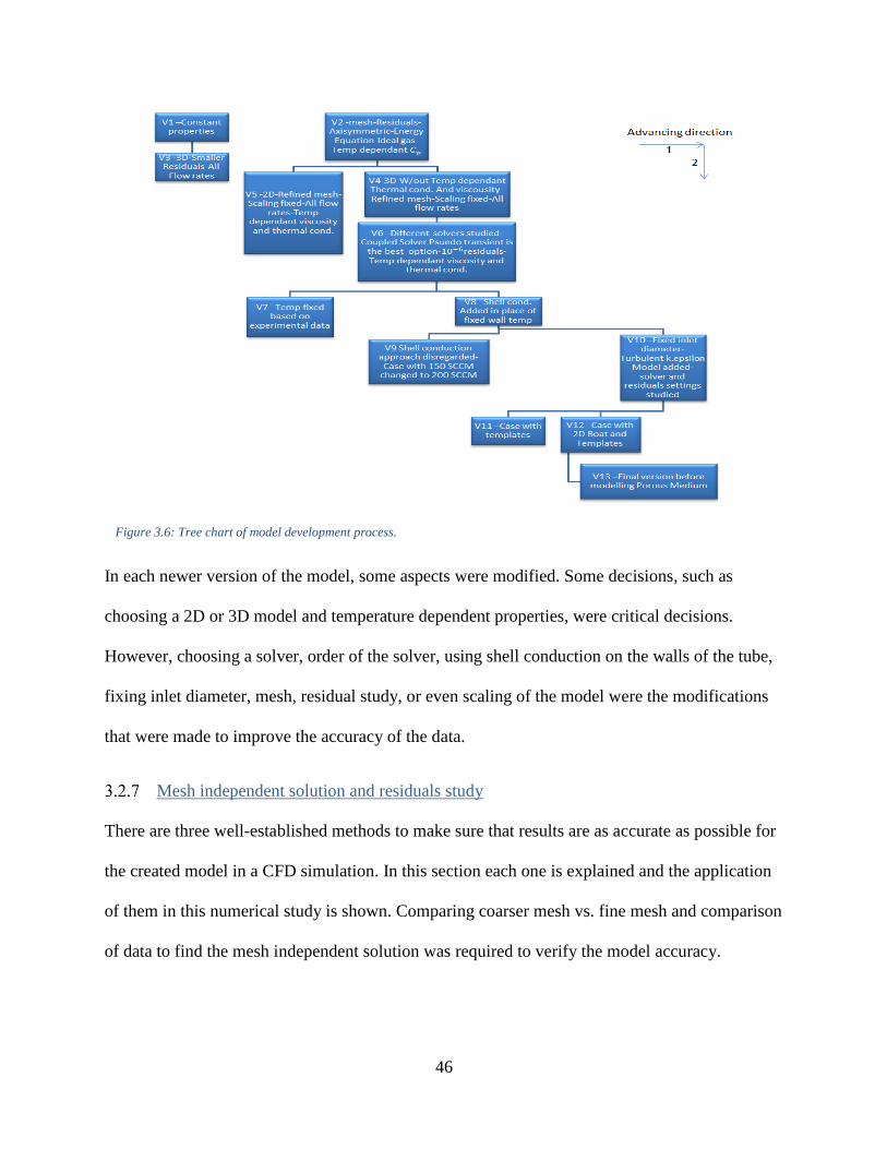
46
In each newer version of the model, some aspects were modified. Some decisions, such as
choosing a 2D or 3D model and temperature dependent properties, were critical decisions.
However, choosing a solver, order of the solver, using shell conduction on the walls of the tube,
fixing inlet diameter, mesh, residual study, or even scaling of the model were the modifications
that were made to improve the accuracy of the data.
Mesh independent solution and residuals study
There are three well-established methods to make sure that results are as accurate as possible for
the created model in a CFD simulation. In this section each one is explained and the application
of them in this numerical study is shown. Comparing coarser mesh vs. fine mesh and comparison
of data to find the mesh independent solution was required to verify the model accuracy.
Figure 3.6: Tree chart of model development process.

47
Finding the mesh independent solution is the most important, among the three. In a CFD
calculation, the conservation of mass, momentum, energy and species are being solved for every
single mesh element, and these equations are being substituted inside a matrix, which solves all
of the equations at the same time. Therefore, a certain number of mesh elements are needed to be
able to capture the small gradients of the studied parameter in a CFD model. An example of this
situation is when we have a very high temperature in the vicinity of lower temperature bulk flow,
similar to the case of the tube furnace in the NBIL. In these types of situations, if the density of
mesh is not high enough, high thermal convection and conduction near the heated wall cannot be
modeled accurately. Similarly, near the areas that flow will be narrowed down and it would
encounter a sudden change in velocity or temperature profile, higher density of mesh is needed.
Examples of such areas can be found at the inlet and outlet of the tube or between the templates
(refer to Section 3.3).
Fully quadrilateral mesh (best mesh quality) with boundary meshing and more dense mesh in
critical points was created to avoid these numerical errors. For example, boundary meshing
technique was used to provide a more dense mesh near the tube walls, inlet and outlet, as well as
near and in between the samples (Fig.3.7). In order to find the mesh independent solution, the
total number of mesh elements was increased from 100K to 500K and 1M mesh elements.
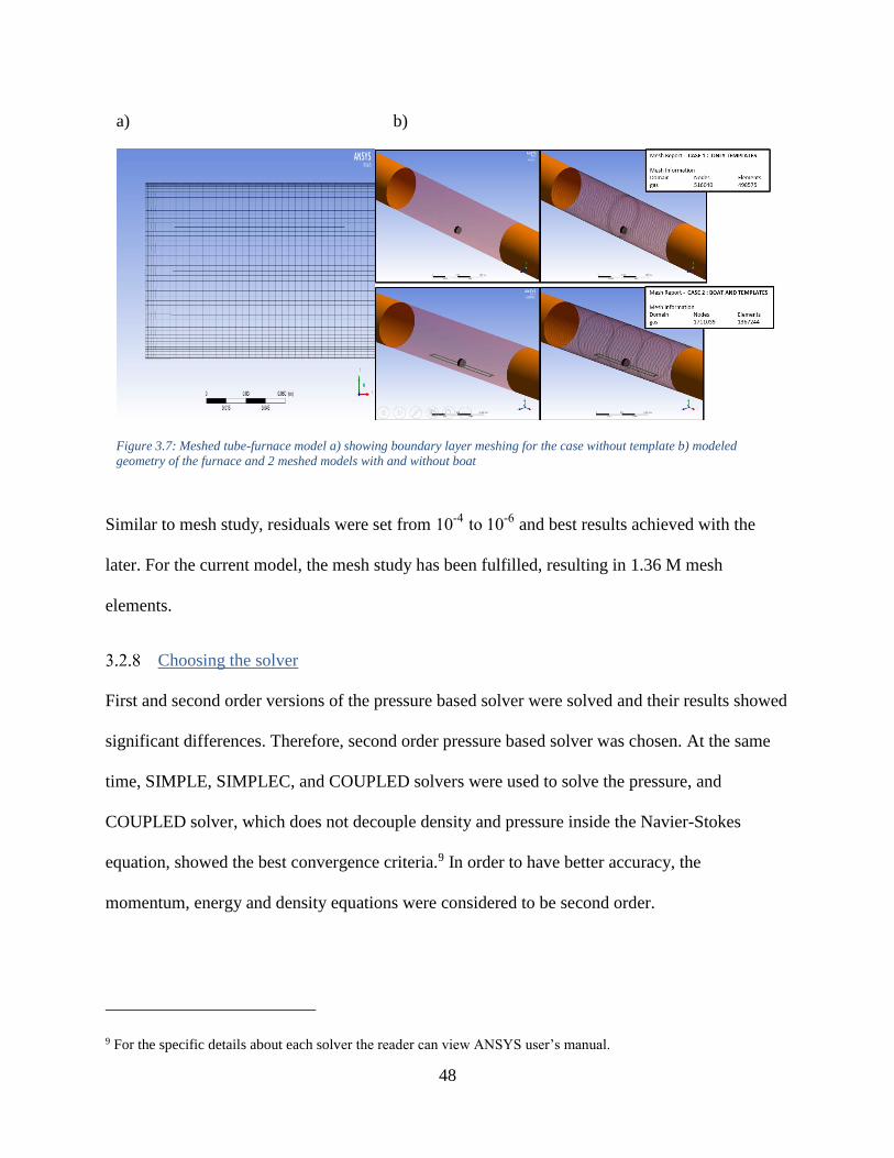
48
Similar to mesh study, residuals were set from 10-4
to 10-6
and best results achieved with the
later. For the current model, the mesh study has been fulfilled, resulting in 1.36 M mesh
elements.
Choosing the solver
First and second order versions of the pressure based solver were solved and their results showed
significant differences. Therefore, second order pressure based solver was chosen. At the same
time, SIMPLE, SIMPLEC, and COUPLED solvers were used to solve the pressure, and
COUPLED solver, which does not decouple density and pressure inside the Navier-Stokes
equation, showed the best convergence criteria.9 In order to have better accuracy, the
momentum, energy and density equations were considered to be second order.
9 For the specific details about each solver the reader can view ANSYS user’s manual.
a) b)
Figure 3.7: Meshed tube-furnace model a) showing boundary layer meshing for the case without template b) modeled
geometry of the furnace and 2 meshed models with and without boat
49
Further modifications to the model
To see the accuracy of the data prediction with CFD simulation, a model without the boat and
templates was used and compared with the acquired data for a similar experimental setup. Figure
3.8a - c show that the numerically obtained data is in a close agreement (< 5% error) with the
experimental data. It also demonstrates the same increase and decrease in the temperature
gradients based on the axial position of the measurement and the value of the studied flow rate.
This step was executed throughout the model development process, to validate the model. This
validation process will be explained in details in the following sections.

50
Figure 3.8: Comparing the temperature from simulation with experimental data. a) 0 sccm experimental flow rate vs. 20
sccm from simulation, b) 500 sccm experimental flow rate vs. 300 sccm from simulation, and c) 500 sccm experimental
flow rate vs. 300 and 500 sccm from simulation.
51
Potential reasons for error in the prediction:
The properties of the gas was simplified in numerical model by assuming a piece-wise linear
change of properties as a function of temperature. Therefore, depending on the operating
temperature, it can create some errors in the prediction of the exact gas properties. Experimental
measurements for temperature in the middle of the tube were obtained in a flow rate of 500
sccm. To prevent the possibility of having an error caused by flow rate difference a model with
500 sccm flow rate was also solved and it was confirmed that comparing 300 sccm with 500
sccm will not have a significant impact on the resulting temperatures. In this section,
experimental results were compared to a 300 sccm inlet flow rate from the simulation (Figure
3.7). Thermal resistivity of the tube has been neglected, which will result in over-predicting
temperature. In addition, temperature is considered to be uniform on each zone. The accuracy
and shape of the sensors may trigger errors. The shape of the sensors can also have an effect on
the flow structure. Number of the points at which the measurements were made are another
potential reason for error. Currently, 5 experimental measurements were made along the heated
range of the tube (from 0.30 m to 1.22 m), however, the results obtained from simulations
contain more than 1000 data points along the same length (more detailed discussion can be found
in Chapter 4).
In Fig. 3.9, temperature plots along the modeled tube furnace are shown. These predicted
temperatures were obtained at the same height as the experimental measurement. A constant
temperature slug is observed in all cases which can move towards the outlet of tube by increasing
the flow rate. The data shows a similar trend in all cases except after 3.78 ft (1.152 m) down the
tube length. As can be seen in the figures, at 1.152 m along the tube and by increasing the flow
rate to 200 sccm and higher, the temperature stays constant, and after this point, temperature

52
does not change by further increasing the flow rate. The suggested reason is the disappearance of
one of the recirculation areas along the tube.
The disappearance of recirculation is shown in Fig. 3.10b. Forced convection decreases near the
outlet of the tube and thereby temperature stays nearly constant.
Figure 3.9: Temperature data along the tube over lines that are 1 inch (a) and 2 inches (b) above the bottom wall of the tube.
a)
b)

53
Model with the sample and boat
In this section, adding the sample and boat to the model is shown and their effect on the
geometry, and flow are inspected. The next step in creating the macro-scale numerical model is
to introduce a simplified version of the Quartz Boat (sample holder) and templates. Three models
were developed for this reason. In the first model (Case 1), only the templates were considered in
the middle of the tube in their actual position. In the second model (Case 2), boat and templates
were considered as 2D shapes and the area in the middle of boat that can hold the samples is
modeled as a hollow horizontal rectangle. Third model (Case 3) was a 3D model of boat and
samples. Figure 3.11 shows mesh independency test for the final model with boat and template.
Figure 3.10: Velocity vector plots showing recirculation zones along the tube at 60 sccm (a), and 200 sccm (b)
a) b)
Recirculation zonesRecirculation zones
Figure 3.11: Mesh independency test - 1367924 mesh elements is confirmed as a reliable number of elements
0.003
0.005
0.007
0.009
0 0.5 1 1.5 2
Ve
loci
ty m
ag
nit
ud
e
(m/
s)
Number of mesh elements (million)
54
Figure 3.12 shows how the velocity is affected by two representations of the boat and templates.
The Third model needed a higher mesh density between the bottom of the tube and bottom wall
of the boat which would make the model more computationally expensive (not shown). First
model (Case 1) could not capture the actual flow structure near the templates. The second and
third case were giving similar results, therefore, Case 2 has been selected among the three cases,
because of its simplicity and accuracy.
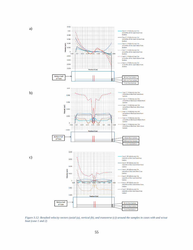
55
Figure 3.12: Resulted velocity vectors (axial (a), vertical (b), and transverse (c)) around the samples in cases with and w/out
boat (case 1 and 2)
a)
b)
c)

56
Presenting the results as a function of flow rate
After going through the steps required for finding the best way to account for the flow structure
around the sample (shown in Section 3.3), this model was solved for all the experimentally
suggested flow rates from Golshadi et al. (20, 40, 60, 80, 100, 200 and 300 sccm). For cases with
20 sccm to 100 sccm flow rates, laminar model and for cases with 200 and 300 sccm flow rates
turbulent k-epsilon model10 was selected. The details of the reasoning behind this change in
viscous model have been explained in Section 3.2.2. In order to see the flow structure and
conditions for velocity and temperature profiles, a cross section in the middle of the tube
(between templates) was considered to be a good representative for measuring the changes in
data caused by different flow rates.
Another aspect that is considered in presenting data, is combining the descriptive statistical
analysis methods and common data presentation tools (such as contour plots, and XY plots for
the results of a variable over a certain line inside the 3D geometry). To have a better
representation of the value of data at each point of the cross section, this task is carried out, using
the following:
Box plots: It is being used to display variation in samples of a statistical population
without making any assumptions of the underlying statistical distribution. It can show
degree of dispersion and skewness in the data, and show outliers.
Histogram: It is a graphical representation of the distribution of data.
10 Refer to viscous model in ANSYS FLUENT user’s manual

57
Standard deviation, median, mean, minimum, maximum and range are all given in a 95%
confidence interval.
Other statistical methods are also suggested in the appendix (Section 8.3.2) that can be used to
explain models with very similar results. However, since the repeatability of data is really high in
this numerical work, statistical methods to this extent does not seem to be a necessity.Combining
the three methods mentioned in bullet points, the reader can find the distribution of each variable
and match it with the color given in contour plot to find the exact location of the data. As shown
in the following figures.
It is shown in Fig. 3.13 that the temperature in the cross section is not changing drastically. The
range of change in temperature from middle of the tube to the bottom is 0.02 kelvins and even
the mean temperature is not changing between different flow rates. This amount of change
cannot have any effect on the next phase of simulation when it will be tried to simulate
deposition of carbon in the pores. The reason is that reaction and diffusion rates will not change
significantly when the change in temperature is this small.

58
Figure 3.13: Contours of temperature for different flow rates on middle cross section of the tube furnace (a), statistical
analysis of temperature data for 100 sccm (Laminar) and 200 sccm (Turbulent) (b) and box plot summarizing all the data and
its trend (c).
20 sccm 40 sccm 60 sccm
80 sccm 100 sccm 200 sccm 300 sccm
a)
b)
c)

59
Figure 3.3b demonstrates the constant temperature region observed in middle of the furnace and
in a 0.47582 ft (145mm) range along tube length. Therefore getting this slight difference in cross
section was predicted beforehand. However, from statistical analysis11 and contours it can be
observed that there is a slight change in temperature range in 200 sccm versus 100 sccm flow
rates which exactly is the transition point that flow changes from being laminar to turbulent. It is
also important to note that due to natural convection and micro forced convections caused by
cross flows and thermal conduction near the wall, temperature contours shown here are semi-
symmetric in a radial manner, thereby the distribution of temperature can be also presented as
shown in Fig. 3.14.
11 Complete statistical analysis report for temperature vs. all flow rates can be found in appendix Section 8.3.2.
Figure 3.14: Temperature versus radial position on the cross section in different flow rates.
Te
mp
era
ture
[k]
Radial Distance from Center [m]
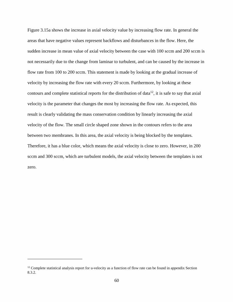
60
Figure 3.15a shows the increase in axial velocity value by increasing flow rate. In general the
areas that have negative values represent backflows and disturbances in the flow. Here, the
sudden increase in mean value of axial velocity between the case with 100 sccm and 200 sccm is
not necessarily due to the change from laminar to turbulent, and can be caused by the increase in
flow rate from 100 to 200 sccm. This statement is made by looking at the gradual increase of
velocity by increasing the flow rate with every 20 sccm. Furthermore, by looking at these
contours and complete statistical reports for the distribution of data12, it is safe to say that axial
velocity is the parameter that changes the most by increasing the flow rate. As expected, this
result is clearly validating the mass conservation condition by linearly increasing the axial
velocity of the flow. The small circle shaped zone shown in the contours refers to the area
between two membranes. In this area, the axial velocity is being blocked by the templates.
Therefore, it has a blue color, which means the axial velocity is close to zero. However, in 200
sccm and 300 sccm, which are turbulent models, the axial velocity between the templates is not
zero.
12 Complete statistical analysis report for u-velocity as a function of flow rate can be found in appendix Section
8.3.2.
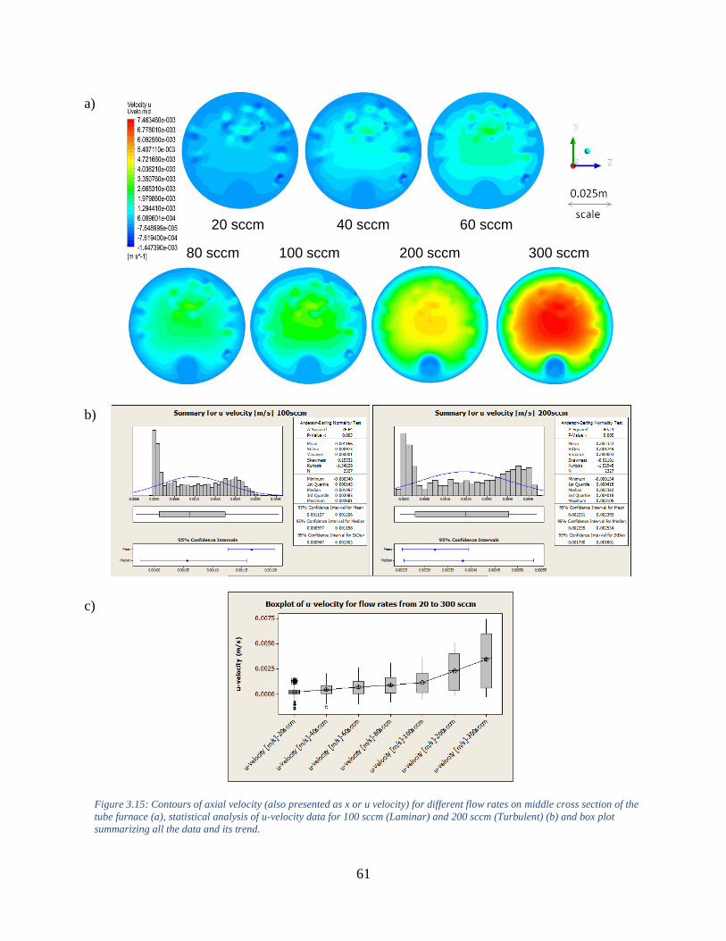
61
Figure 3.15: Contours of axial velocity (also presented as x or u velocity) for different flow rates on middle cross section of the
tube furnace (a), statistical analysis of u-velocity data for 100 sccm (Laminar) and 200 sccm (Turbulent) (b) and box plot
summarizing all the data and its trend.
20 sccm 40 sccm 60 sccm
80 sccm 100 sccm 200 sccm 300 sccm
a)
b)
c)

62
The standard deviation and mean vertical velocity are extracted from the statistical data13 of 100
sccm flow rate and are shown in Fig. 3.16 (their values are 4.854 mm/s and 2.340 mm/s,
respectively). Therefore, it should be noted that the data for the vertical component of velocity is
subject to a lot of fluctuations. In addition, the box plot shows many outlier data points for each
flow rate. There can be two reasons for this observation: 1) Cross flows caused by natural
convection and buoyancy effects (sudden changes in density); 2) there may be an error or
skewed mesh element which prevents FLUENT from giving a precise value for some mesh
elements. The second reason is less likely because the quadrilateral meshing technique has been
used to mesh the tube furnace geometry and much lower density of skewed meshes are expected
in such a structure. Thereby, the first possibility is more likely to be the case. Random cross
flows will occur due to the buoyancy effect and this can create a non-uniform result. Other
interesting observation from the contours and box plot is the decrease in v-velocity when the
model changes from laminar to turbulent between 100 and 200 sccm. Since turbulent flow has a
more disturbed flow pattern, this decrease in mean vertical velocity can be considered as a
logical consequence of better mixing. V-velocity is at maximum in the center of the tube for all
flow rates. The suggested reason is that this point that has the highest distance from the heated
tube walls and therefore has the lowest density changes (disturbances).
13 Complete statistical analysis report for v-velocity as a function of flow rate can be found in appendix Section
8.3.2.
63
Figure 3.16: Contours of vertical velocity (v) for different flow rates on middle cross section of the tube furnace (a), statistical
analysis of v-velocity data for 100 sccm (Laminar) and 200 sccm (Turbulent) (b) and box plot summarizing all the data and its
trend (c)
20 sccm 40 sccm 60 sccm
80 sccm 100 sccm 200 sccm 300 sccm
a)
b)
c)

64
Looking at the velocity vectors and streamlines presented in Fig. 3.17 and Fig. 3.3c, the
buoyancy effect, which opposes gravity and recirculates back to the bottom of the tube, can be
observed.
Lastly, transverse (w) component of velocity is shown in Fig. 3.18. As it was also observed v-
velocity, by transition from laminar to turbulent; there is a small decrease in the value of w-
velocity. Mean value is close to zero (approximately -0.000035 m/s) and standard deviation is
0.0033 m/s. It means that the data covers a large variation, which was predictable looking at the
contour plots and seeing the distribution of velocity. Bottom right and top left corners are
showing recirculation in reversed direction and bottom left and top right are opposing this
movement.
Figure 3.17: Velocity vectors in the middle cross section of tube furnace (a), streamlines, showing the cross flows (b), and
laminar flow (c) vs. turbulent flow (d).
a)
c)
b)
d)

65
Figure 3.18: Contours of transverse velocity (w) for different flow rates on middle cross section of the tube furnace (a).
Statistical analysis of w-velocity data for 100 sccm (Laminar) and 200 sccm (Turbulent) (b) and box plot summarizing all the
data and its trend (c)
20 sccm 40 sccm 60 sccm
80 sccm 100 sccm 200 sccm 300 sccm
a)
b)
c)

66
No significant fluctuations observed near the templates as a function of flow rate. Unlike v-
velocity, by increasing flow rate from 20 to 100, the value of z velocity is slightly decreasing and
by the change to turbulent it decreases further and then continues to decrease again14.
When the CVD process is in progress, velocity distribution around the sample can affect the
anticipated rate of diffusion inside the pores of the template. Therefore, knowing the exact
macro-scale flow structure is of great importance (Wang 1989).
Conclusion
Symmetric and fairly constant temperatures were observed in the middle of the tube furnace.
This constant temperature is not significantly affected by the disturbances in the flow and, on the
contrary, they help to keep temperature constant. On the other hand, velocity showed a direct
relation with inlet flow rate, especially the axial velocity. However, v and w component were
governed by buoyancy effects and flow being turbulent or laminar. Analysis of the results
suggests that the threshold of changing to turbulent is higher than 300 sccm and the deposition
change that we are observing in the experiments is not related to a change in flow regime.
Therefore, in order to find the experimental result, a more robust numerical model should be
chosen and tested to measure the effect of buoyancy related disturbances or cross flows on the
carbon mass deposition. The model development is described in the following chapter.
14 Complete statistical analysis report for w-velocity as a function of flow rate can be found in appendix section
8.3.2.

67
Chapter 4

68
4 Model Validation and Development
Governing equations and gas properties
Three types of numerical models were developed to describe the physical CVD process, starting
with the most simple (basic assumptions) to the more complex (refined assumptions). The first
type of model assumes a steady 3D laminar flow inside the tube furnace with constant density,
viscosity and thermal conductivity. The outcome of this model is similar to the simple problem
of developing flow inside a tube. This is due to the fact that the gas properties are constant in this
model. Thereby, the model cannot show the change in density, because the buoyancy effects are
not considered. The second type of model utilizes the Boussinesq approximation for buoyancy
driven flows, which is applied to a given constant density. This is a good approximation method
for a nearly incompressible flow and when considering density variations due to small changes in
temperature. However, temperature differences in our domain are large (25°C to 700°C) so we
expect the use of Boussinesq model will induce error. Furthermore, this model cannot be used
with species calculations, combustion, or reacting flows. The third type of model incorporates
temperature-dependent properties. Since this method includes temperature-dependent viscosity
and thermal conductivity, it incorporates buoyancy and flow shear effects, and thereby provides
the most accurate representation of the physical system. The latter model employs piece-wise
linear approximation for the temperature-dependent variables. Ethylene and helium temperature-
dependent properties (Holland, Eaton, and Hanley 1983; Rogers and Mayhew 1994) were used
to account for density variations.
Four numerical models were developed to describe the physical CVD process, starting with the
most simple (basic assumptions) to the more complex (refined assumptions), as summarized in
Table 4.1. In previous work, we showed that 3D modeling and temperature dependent properties

69
provide a more accurate representation of the physical system (Vahedein and Schrlau 2015).
Therefore, all models in this work (M-1 to M-4) are three dimensional and incorporate piece-
wise linear approximations for temperature-dependent viscosity and thermal conductivity to
account for buoyancy and flow shear effects in the physical system (Rogers and Mayhew 1994).
Model M-1, the simplest of the four models, assumes single-species thermo-fluid flow in the
tube furnace, i.e., the only gas flowing in the system is the carbon-carrying component of the
precursor gas in the actual physical system: ethylene. Building upon model M-1, model M-2
represents single-species thermo-fluid flow in the presence of the boat and templates inside the
tube furnace. Increasing in complexity to better represent the actual physical system, model M-3
assumes multi-species thermo-fluid flow in the furnace tube, i.e., the precursor gas consists of
ethylene diluted in helium. The closest representation of the physical system of the four models,
model M-4, assumes multi-species thermo-fluid flow and ethylene species consumption at the
template surface.
Table 4.1. Specifications of the four TB-CVD models.

70
Many publications have dealt with mixed convection heat transfer for laminar flow in a
horizontal duct (Patankar, Ramadhyani, and Sparrow 1978; Shannon and Depew 1968;
Choudhury and Patankar 1988; Bergles and Simonds 1971; Newell and Bergles 1970). The
secondary motion created in the tube distorts the isothermal parabolic velocity profile, which
influences its stability. Reynolds number, Grashof number and Rayleigh number were tested in
this work, which confirmed the flow in tube reactor is prone to mixed convection. In addition, as
discussed later, Boltzmann number was calculated and it was found that the effect of heat
transfer due to radiation is negligible.
Since this work falls in the continuum regime (Knudsen number << 1), the following forms of
the continuity equation were applicable. These forms are shown as Equation 4.1 (general
differential form of continuity equation, used in M-1 and M-2) and Equation 4.2 (convection-
diffusion equation for the 𝑖𝑡ℎ species, used in M-3 and M-4):
∂ρ
∂t + ∇∙(ρv̅) = Sm (4.1)
In Equation 1, 𝜌 is density, 𝑡 is time. The terms on the left are representing the unsteady and
convection parts of the continuity equation. Sm is the amount of mass that is generated, which is
Sm=0 in the case of models M-1 to M-3. As it will be explained later in the Boundary Conditions
section, M-4 has a perfectly absorbing boundary condition on the template walls, which can be
interpreted as a sink for ethylene mass. Therefore, for model M-4, Sm will not be equal to zero
and, instead, will be determined by the rate of consumption of ethylene in Equation 4.2 (i.e. Si).
Conservation equations are solved in two forms in this work: single-species (i.e., models with
ethylene as the inlet gas; models M-1 and M-2), and multi-species (i.e., models with ethylene
and helium mixture as the inlet gas; models M-3 and M-4).

71
∂
∂t(ρYi) + ∇∙(ρv̅Yi) = Si + Ri - Yi∇∙(DAB∇xi) (4.2)
For models M-3 and M-4, Equation 4.2 will be solved for N-1 species, where N is the total
number of fluid phase chemical species present in the system (N=2). Reactions are not modeled
in this work, therefore, the reaction source term, R, is equal to zero. Since, there are only two
species entering the system, diffusive flux of species i is represented with a binary diffusion
term, Yi∇.(DAB.∇xi), in which DAB is the binary diffusion coefficient calculated using kinetic
theory and 𝑥𝑖 is the mole fraction of the ith species. Since the steady state solution will be
employed in this work, ∂ρ
∂t and further mentioned derivatives with respect to time will be equal to
zero.
DAB is calculated using the Chapman-Enskog theory (Chapman and Cowling 1970). This theory
is accurate within 8% of the exact value and leads to Equation 4.3 to calculate diffusion
coefficient.
D = 1.86×10
-3 T32 (
1
M1 +
1
M2)
12
Pσ122 Ω
(4.3)
In this equation, M1 and M2 represent the molecular weight of the first and second species,
respectively, and T is the absolute temperature in degrees of Kelvin. The parameters, σ12 and Ω,
are molecular properties characteristic of the Chapman-Enskog theory (Chapman and Cowling
1970) that calculate collision diameter and the dimensionless property pertaining to the species
interaction, respectively. Parameter σ12 can be calculated by extracting the 𝜎 values for each of
the interacting species from experimental results known as Lennard-Jones potential parameters
(J. E. Jones 1924) and averaging them. On the other hand, Ω, which is also known as the

72
collision integral, can be extracted from Hirschfelder et al. (Joseph O. Hirschfelder 1955) for
ethylene and helium.
The differential form of momentum conservation is described by Equation 4.4:
∂
∂t(ρv̅) + ∇∙(ρv̅v̅) = -∇p + ∇∙(τ̅) + ρg̅ + F̅ (4.4)
Here, 𝜏̅ is the stress tensor and is given as:
τ̅ = μ [(∇v̅ + ∇v̅T) - 2
3∇∙v̅I] (4.5)
The effect of volume dilation can be viewed in the right hand side of Equation 4.5 (𝐼 is unit
tensor).
The differential form of the energy equation is described by:
∂
∂t(ρE) + ∇(v̅(ρE + P)) = ∇∙ (keff∇T - ∑ hj (Yj∇∙(DAB∇xj))+ (τ̅eff∙v̅)j )+ Sh (4.6)
The left side of Equation 4.6 shows the rate of change for kinetic and internal energy (E is the
fluid specific internal energy). On the right side of Equation 4.6, keff is the effective thermal
conductivity. In the parenthesis, energy transferred by conduction, species diffusion, and viscous
dissipation are shown respectively. Sh is any generated energy such as from chemical reactions
and so on. None of the four models will include the generated energy source term and only
models M-3 and M-4 will include the terms pertaining to species diffusion.
The pressure-based method employs a set of equations known as projection method equations
(Guermond, Minev, and Shen 2006). Since the flow is mixed flow (not Eulerian) and
compressible, the coupled form of this solver method is applicable. The coupled algorithm solves

73
the momentum and pressure-based continuity equations together. The full implicit coupling is
achieved through an implicit discretization of pressure gradient terms in the momentum
equations, and an implicit discretization of the face mass flux, including the Rhie-Chow pressure
dissipation terms (Rhie and Chow 1983). Coupled AMG solver is used to solve linear transport
equations using implicit discretization from a coupled pressure-based scheme.
To summarize the discussion above, a 3D steady state, second order, pressure-based, coupled
solver with pseudo automatic time-stepping and temperature-dependent properties of the inlet
gas (ethylene) or mixture gas (ethylene and helium) was utilized in the current study.15
Boundary conditions
The boundary conditions for the four models are shown in Fig. 4.1. Two stages of the furnace (A
and E) are considered to be adiabatically isolated and, therefore, act like perfect insulators. The
walls of stages B, C and D are assumed to be isothermal and have a constant temperature
boundary condition.
In the tube furnace that is used in our lab, the constant temperature setpoints for stages B, C, and
D are 680°C, 700°C, and 680°C, respectively. From experimental measurements, it was found
that the temperatures on the inside wall of tube were approximately 12°C lower than the
setpoints. The difference between the furnace setpoints and the temperatures inside the tube is
due to the series of thermal resistances caused by the airgap between the furnace heaters and
outer walls of the tube, and the wall thickness of the ceramic tube. The inlet boundary is defined
as a mass flow inlet boundary condition perpendicular to the cross sectional area of the inlet,
15 More detailed governing equations and multi-phase model equations are available in appendix. These models
were tried but was not decided as the most accurate representation of the TB-CVD process.

74
where mass flow ranges from 3.93x10⁻⁷ kg/s for 20 sccm flow rate to 5.9x10⁻⁶ kg/s for 300
sccm for M-1 and M-2 and from 8.01×10⁻⁸ kg/s for 20 sccm to 1.2×10⁻⁶ kg/s for 300 sccm for
M-3 and M-4 (Discussion of differences provided later in the Results and Discussion section).
Therefore, pressure and velocity are calculated by the CFD code at the inlet. In numerical
simulations, all parameters except flow rate were kept constant to mimic the physical
experimental system.
As illustrated in Fig. 4.1, models M-3 and M-4 have zero diffusive flux boundary conditions
resulting from solving transport equation in conjunction with continuity and momentum
equations (No penetration boundary condition at the walls and zero diffusive flux at the outlet).
Model M-4 includes an additional boundary condition, which is the perfectly absorbing
boundary condition of ethylene for all the template walls, defined as: CC2H4 = 0. With this
method, the effect of decomposition of ethylene and deposition of carbon was replaced with a
perfect sink of ethylene on the templates. Therefore, in model M-4, it has been assumed that the
TB-CVD process is mass transport limited.
Since the temperature difference is noticeably high between the inlet gas and the middle stage of
the furnace, an unsteady mixed convection condition in the horizontal tube reactor was expected
Figure 4.1: Schematic representation of the boundary conditions for the TB-CVD tube furnace. Boundary conditions only
pertaining to model M-4 are indicated with single asterisks (*). Boundary conditions pertaining to the species concentration
are indicated with double asterisks (**).

75
(I. Guillén 2014; Ingham and Merkin 1981; Jain and Lohar 1979). Additionally, due to the
sudden expansion of the inlet to the tube, recirculation near the inlet was expected. However, the
Reynolds number calculated for the tube (Re = 73 to 1100 – laminar regime) shows that these
disturbances will be dampened throughout the flow.
The outlet boundary condition has been set to zero gauge pressure. The following equation
shows the calculation method of the outlet boundary pressure. This calculation method prevents
the arising pressure calculation errors near the outlet region such as backflows induced by
numerical error. Equation 7 uses the average value of pressure on the centroid of mesh elements
adjacent to the outlet wall and the exit pressure, and finally adds it to the partial pressure
difference:
pf = 0.5(p
c + p
e) + dp (7)
Here, 𝑝𝑐 is the pressure of the interior mesh element, 𝑝𝑒is the specified exit pressure at the
neighbouring mesh element to the exit, and dp is the difference between specified pressure and
the latest average pressure for the boundary. This value is defined as follows:
dp = (pe -
∑ 0.5(pc + pe)(Area)
i=nface
i=1
∑ Areai=nface
i=1
) (4.8)
In Equation 4.9, constant buoyancy forces for buoyancy driven hydrostatic flow are shown,
which are independent of the flow speed. This condition was observed in the middle region of
the tube furnace:

76
In the case where two fluids exist in the control volume, ρref
is calculated by considering 𝑋𝑐2ℎ4
and 𝑋𝐻𝑒, which are the molar concentrations of ethylene and helium, respectively.
Validation
Setting up a 2D numerical model was the first choice in this work to reduce the computational
cost. Creating a 2D axisymmetric solution was not possible for two reasons: The boat and template
were placed on the bottom wall of the tube, and gravity was perpendicular to the axis of symmetry.
Therefore, a regular 2D case simplifying the tube boundary conditions was created and compared
to a 3D case. As shown in Fig. 4.2a, it can be observed that both 2D and 3D models could capture
the temperature variations and the parabolic shape of the temperature profile close to the middle
of the tube. From Fig 4.2b it can be noted that this parabolic shape is caused by the velocity field
recirculations in the middle zone of the tube furnace. On the other hand, Fig. 4.2b shows the
resultant velocity magnitude vectors for 2D and 3D case in the region in vicinity of the boat and
templates. It can be observed that recirculating velocity vectors (as can be viewed in 2D case) are
replaced by vectors uniformly directed towards the upper tube wall, meaning that the direction of
flow is towards upper wall. Upon closer inspection of streamlines in the middle cross-section and
in the entire tube (Figs. 4.2c, d), it can be inferred that the 2D case cannot capture the recirculations
perpendicular to the direction of the flow and, therefore, cannot correctly predict temperature
profiles and velocity patterns.
Buoyancy force on fluid parcel = (ρ - ρref
)g
ρref
= (Xc2h4ρ
c2h4 + XHeρ
He) (4.9)
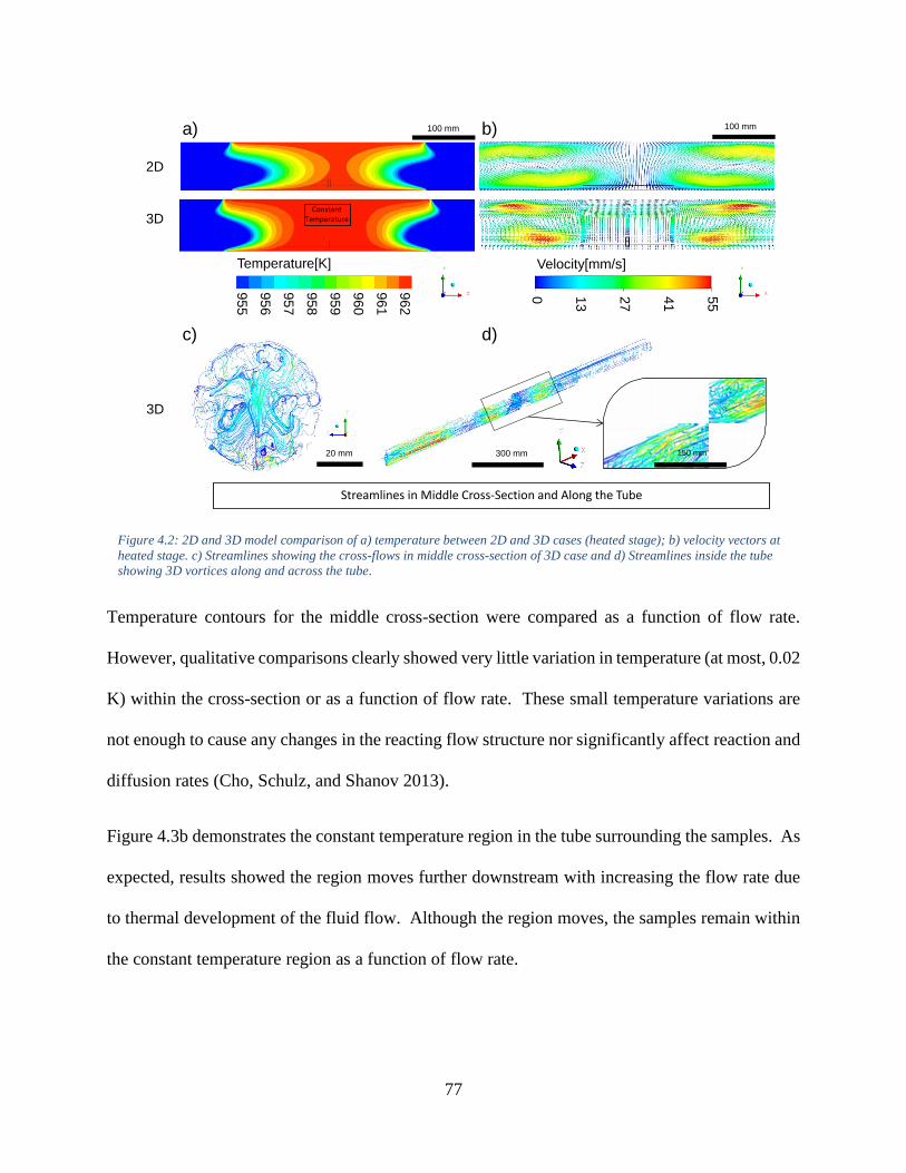
77
Temperature contours for the middle cross-section were compared as a function of flow rate.
However, qualitative comparisons clearly showed very little variation in temperature (at most, 0.02
K) within the cross-section or as a function of flow rate. These small temperature variations are
not enough to cause any changes in the reacting flow structure nor significantly affect reaction and
diffusion rates (Cho, Schulz, and Shanov 2013).
Figure 4.3b demonstrates the constant temperature region in the tube surrounding the samples. As
expected, results showed the region moves further downstream with increasing the flow rate due
to thermal development of the fluid flow. Although the region moves, the samples remain within
the constant temperature region as a function of flow rate.
Figure 4.2: 2D and 3D model comparison of a) temperature between 2D and 3D cases (heated stage); b) velocity vectors at
heated stage. c) Streamlines showing the cross-flows in middle cross-section of 3D case and d) Streamlines inside the tube
showing 3D vortices along and across the tube.
100 mm
2D
3D
20 mm 300 mm
3D
150 mm
Streamlines in Middle Cross-Section and Along the Tube
Constant Temperature
100 mm
Temperature[K]
956
955
957
958
959
960
961
962
Velocity[mm/s]
0 13
27
41
55
a) b)
c) d)

78
To check the accuracy of the data predicted with CFD simulation, a 3D model of tube without the
boat and templates was developed and compared with experimental data from the physical system.
Thermocouples were used to collect temperature data from several positions inside the furnace as
a function of the axial position from the center of the tube, as shown in Figure 4.3c. The results
of the comparison show the temperature profile in the vicinity of the sample predicted by
simulation agrees closely with the experimental data. It can be observed that the trend of
temperature decrease or increase based on the position in the tube is captured in this numerical
model.
To make sure that radiation heat transfer can be neglected with respect to the contribution of
convective heat flux, the non-dimensional Boltzmann number, Bo, was calculated (Bo=16.875).
Since this value is 16 times larger than 1, radiation has a negligible contribution to heat transfer
compared to the convective term.
Figure 4.3: Contours of temperature on: middle cross-section (a), and along the tube, showing constant temperature slug (b).
Panel c) temperature from experimental measurement versus temperature data from simulation.
b)
a)
0.150.100.050.00-0.05-0.10-0.15
690
680
670
660
650
Position from middle of tube furnace [m]
Tem
pra
ture
[°C
]
Temperature Vs Length - 25.4 mm Above Bottom Wall
Temperature Vs Length - 38.1 mm Above Bottom Wall
Temperature Vs Length - 25.4 mm Above Bottom Wall(simulation)
Temperature Vs Length - 38.1 mm Above Bottom Wall(simulation)
V ariable
Area in vicinity of templates
0.02m
C)
79
Modeling Considerations
Modeling the boat and templates
The next step in creating the macro-scale numerical model was to introduce a simplified version
of the Quartz Boat (sample holder) and templates. Therefore, three meshed cases were created
and solved with the aforementioned boundary conditions: Case 1 consisted of the boat and
templates in 3D; Case 2 consisted of a 2D rectangular boat and 2D circle-shaped walls as
templates; Case 3 consisted of 2D circle-shaped templates and no boat. Case 1 was solved and it
was observed that a unique flow structure exists around the templates. However, Case 1 was
computationally expensive. To reduce computation time, 2D representations of the boat and
templates were created (Case 2). It was found that the simplified model in Case 2 could
accurately replicate the same unique flow structure as Case 1 (This unique flow structure is
shown in Figs. 4.5 and 4.6). To further reduce the computational expense, a mesh structure for
2D templates without any mesh for the boat was created (Case 3). While Case 3 was less
computationally expensive than Case 1 and Case 2, the flow structure differed significantly.
Therefore, Case 2 was used as the most simplified and accurate representation of the boat and
templates to calculate the flow structure near the templates in M-2 to M-4.
Meshing technique
Figure 4.4a shows the 3D meshed tube furnace with the 2D representations of the boat and
templates (Case 2) at the center of the tube. For initial value (marching) problems governed by
the finite-difference approximations of linear partial differential equations, Lax’s equivalence
theorem needs to be satisfied to prevent the possibility of having stability or consistency errors in
the final numerical solution. Mesh independency and residual convergence studies were
conducted for all models to account for the Lax and Richtmyer Theorem (Lax and Richtmyer

80
1956). A convergence criteria in the order of 10−6 was selected as the convergence criteria for
continuity, momentum, energy and species conservation differential equations. The quadrilateral
meshing technique was used throughout the tube furnace using copper and pave mesh
techniques. Boundary meshing and more compact mesh grids were created at critical points such
as near the walls of the tube, at the inlet and outlet, and between templates. For example, Fig.
4.4b shows the boundary layer meshing near the inlet.
In order to find the mesh independent solution, the total number of mesh elements was increased
from 100K to 2M mesh elements by applying mesh refinement techniques based on the
momentum convergence criteria. By comparing the velocity magnitude in the middle cross
section as a function of mesh elements, the mesh independent solution was obtained with 1.36M
mesh elements.
Results and discussion
To determine how process conditions affect thermo-fluid behavior within the reactor, four 3D
macro-scale models were created and numerically solved in ANSYS® FLUENT® on an HP Z620
Figure 4.4: Model mesh structure of the TB-CVD tube furnace. Perspective view of the model mesh structure near the boat
and templates inside the tube furnace (a). 2D projected view of the 3D mesh near the inlet, showing boundary layer meshing
near the walls (b).

81
workstation (4-core, 2.1 GHz, 16 Gb RAM). Contour plots of u, v and w velocity components in
the middle cross-section at the position of the templates (Fig. 4.5) and along the entire tube axis
(Fig. 4.6) were generated. For each model, the mean, range, and standard deviation of the
velocity components, and the circulation strength in the middle cross-section and longitudinal
section of the tube furnace were reported as a function of flow rate (Table 4.2). This data was
collected from 2,300 cross-sectional and 25,221 longitudinal data points with 95% confidence
interval for standard deviation. The numerical results and observations from models M-1 to M-4
are summarized below, along with a short discussion of their advantages, disadvantages, and
computational cost. Comparisons between the models are then discussed to elucidate how
various process conditions affect thermo-fluid flow in the furnace.
Description of model results
Numerical solutions to simulate the TB-CVD process that is being used in our lab to
manufacture carbon nanotubes are presented in an ordered manner. These models are sorted
based on the accuracy level. This development of the model was necessary and the results are
showing the effect of considering each of the properties, such as: the template and boat in model
M-2, species concentrations by introducing helium to the system in model M-3 and having
consumption of ethylene on the templates in model M-4.
In the statistical data presented in Table 4.2, standard deviations are generally higher than the
mean values, which infer that the dispersion in data is high and the mean value does not perfectly
represent the velocity in the whole cross section. The velocity values should be observed and
analyzed in specific regions of interest inside the cross section. The combination of contour plot
data, and mean and standard deviation in the cross section gives the best possible insight of the
velocity fields near the templates.
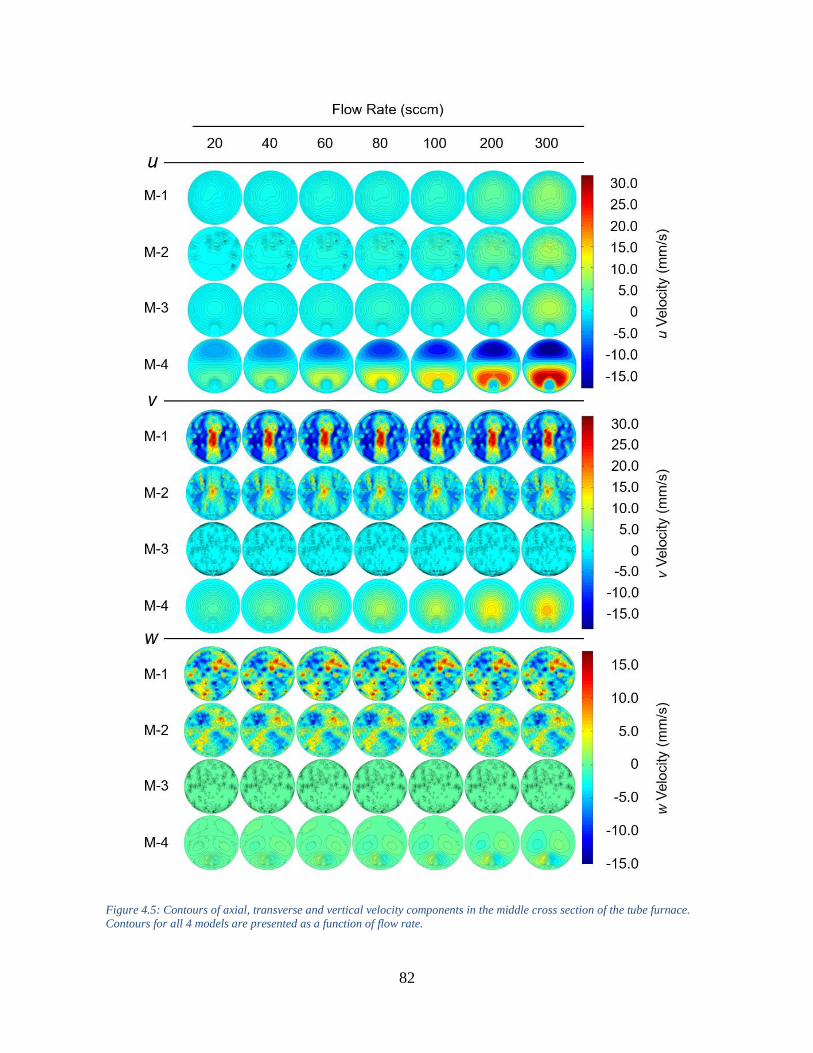
82
Figure 4.5: Contours of axial, transverse and vertical velocity components in the middle cross section of the tube furnace.
Contours for all 4 models are presented as a function of flow rate.

83
Model M-1: A single-species, steady state and temperature dependent model representing the
CVD tube furnace. Results in Table 4.2 show the velocity components, u, v and w, as a function
of flow rate, range from u20 = 0.220 ± 0.165 mm/s, v20 = 3.183 ± 9.880 mm/s, w20 = 0.370 ±
4.510 mm/s to u300 = 3.370 ± 0.165 mm/s, v300 = 3.243 ± 9.870 mm/s, w300 = 0.330 ± 4.498
mm/s. As expected, the u component of velocity increases as a function of flow rate. However,
the v and w components do not significantly change with increasing flow rate. Due to mixed
convection, circulation occurs in the middle cross section and longitudinal section, ranging in
circulation strengths from Γ20 = 114.7 cm2/s to Γ300 = 90.1 cm2/s and from Γ20 = 4241.3 cm2/s to
Γ300 = 3960.0 cm2/s, respectively. From inspection, and relative to their scale, circulation in the
middle cross section and longitudinal section do not significantly change as a function of flow
rate. At the middle cross section, the radial temperature profile remains nearly constant (Tave =
961.50 ± 0.02 K) for all the flow rates. A 200 mm long constant temperature slug (Tave = 960.80
± 0.75 K) also extends in the axial direction, with its center-point located between the templates
at a flow rate of 20 sccm. The center-point of temperature slug moves at most 10 mm from
middle cross section towards the outlet when the flow rate is increased from 20 to 300 sccm.
The numerical solution was obtained in 2 hours.
Model M-2: A single-species, steady state, and temperature-dependent model representing the
CVD tube furnace, which includes the boat and templates. Results in Table 4.2 show the velocity
components, u, v and w, as a function of flow rate, range from u20 = 0.240 ± 0.165 mm/s, v20 =
2.329 ± 4.853 mm/s, w20 = -0.039 ± 3.332 mm/s to u300 = 3.500 ± 2.886 mm/s, v300 = 2.440 ±
4.881 mm/s, w300 = -0.046 ± 3.310 mm/s. As expected, the u component of velocity is increasing
as a function of flow rate. However, v and w components do not significantly change with
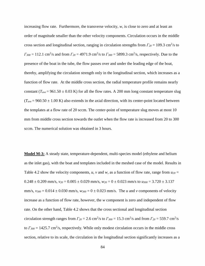
84
increasing flow rate. Furthermore, the transverse velocity, w, is close to zero and at least an
order of magnitude smaller than the other velocity components. Circulation occurs in the middle
cross section and longitudinal section, ranging in circulation strengths from Γ20 = 109.3 cm2/s to
Γ300 = 112.1 cm2/s and from Γ20 = 4971.9 cm2/s to Γ300 = 5899.3 cm2/s, respectively. Due to the
presence of the boat in the tube, the flow passes over and under the leading edge of the boat,
thereby, amplifying the circulation strength only in the longitudinal section, which increases as a
function of flow rate. At the middle cross section, the radial temperature profile remains nearly
constant (Tave = 961.50 ± 0.03 K) for all the flow rates. A 200 mm long constant temperature slug
(Tave = 960.50 ± 1.00 K) also extends in the axial direction, with its center-point located between
the templates at a flow rate of 20 sccm. The center-point of temperature slug moves at most 10
mm from middle cross section towards the outlet when the flow rate is increased from 20 to 300
sccm. The numerical solution was obtained in 3 hours.
Model M-3: A steady state, temperature-dependent, multi-species model (ethylene and helium
as the inlet gas), with the boat and templates included in the meshed case of the model. Results in
Table 4.2 show the velocity components, u, v and w, as a function of flow rate, range from u20 =
0.248 ± 0.209 mm/s, v20 = 0.005 ± 0.029 mm/s, w20 = 0 ± 0.023 mm/s to u300 = 3.720 ± 3.137
mm/s, v300 = 0.014 ± 0.030 mm/s, w300 = 0 ± 0.023 mm/s. The u and v components of velocity
increase as a function of flow rate, however, the w component is zero and independent of flow
rate. On the other hand, Table 4.2 shows that the cross sectional and longitudinal section
circulation strength ranges from Γ20 = 2.6 cm2/s to Γ300 = 15.3 cm2/s and from Γ20 = 559.7 cm2/s
to Γ300 = 1425.7 cm2/s, respectively. While only modest circulation occurs in the middle cross
section, relative to its scale, the circulation in the longitudinal section significantly increases as a

85
function of flow rate. At the middle cross section, the radial temperature profile remains nearly
constant (Tave = 961.50 ± 0.01 K) for all the flow rates. A 250 mm long constant temperature slug
(Tave = 961.00 ± 0.50 K) also extends in the axial direction, with its center-point located between
the templates at a flow rate of 20 sccm. The center-point of temperature slug moves at most 10
mm from middle cross section towards the outlet when the flow rate is increased from 20 to 300
sccm. The numerical solution was obtained in 8 hours.
Model M-4: A steady state, temperature-dependent, multi-species model with boat and
templates included in the meshed case and consumption of ethylene at the templates. This model
is the closest representation to the physical TB-CVD process. Results in Table 4.2 show the
velocity components, u, v and w, as a function of flow rate, range from u20 = 0.855 ± 2.217
mm/s, v20 = 1.370 ± 1.220 mm/s, w20 = 0.001 ± 0.193 mm/s to u300 = 7.451 ± 13.378 mm/s, v300 =
5.967 ± 5.555 mm/s, w300 = 0.008 ± 1.211 mm/s. All velocity components increase as a function
of flow rate. For flow rates less than 100 sccm, the vertical component of velocity, v, has the
same order of magnitude as axial velocity (e.g., u40 = 1.511 ± 3.638 mm/s, v40 = 2.174 ± 1.930
mm/s). However, for higher flow rates, axial velocity increases at a faster rate than the v and w
components (e.g., u300 = 7.451 ± 13.378 mm/s, v300 = 5.967 ± 5.500 mm/s).
Longitudinal and cross-sectional recirculations were observed, as shown in Fig. 4.6. Due to
mixed convection and species consumption, as highlighted by the velocity vectors in Fig. 4.6,
circulation occurs in the middle cross section and longitudinal section, ranging in circulation
strengths from Γ20 = 12.1 cm2/s to Γ300 = 74.3 cm2/s and from Γ20 = 625.0 cm2/s to Γ300 = 1601.8
cm2/s, respectively. These results show circulations in both sections are relatively increasing as a
86
function of flow rate. At the middle cross section, the radial temperature profile remains nearly
constant (Tave = 961.50 ± 0.01 K) for all the flow rates. A 250 mm long constant temperature slug
(Tave = 961.00 ± 0.50 K) also extends in the axial direction, with its center-point located between
the templates at a flow rate of 20 sccm. The center-point of temperature slug moves at most 10
mm from middle cross section towards the outlet when the flow rate is increased from 20 to 300
sccm. The numerical solution was obtained in 9 hours.

87

88
The effect of modeling parameters on thermo-fluid behavior
In previous experiments conducted by others, buoyancy driven recirculations were observed in
the cross sections along and perpendicular to the flow in a tube furnace (Fotiadis and Jensen
1990; Giling 1982; Chiu, Richards, and Jaluria 2000). These recirculations are caused by
buoyancy driven flow due to gas density variations in the center of the tube (Fotiadis and Jensen
1990). Longitudinal rolls and cross flows are indications of having mixed convection in the
system, which can create turbulence, induce better mixing, and facilitate faster reactions (Sornek,
Dobashi, and Hirano 2000). In this work, similar buoyancy effects in the tube furnace were
observed in all models. In the following sections, models M-1, M-2, M-3 and M-4 were
compared to determine the differences in temperature and mass flow rate, and how the boat and
templates, gas composition and species consumption affected thermo-fluid flow in the TB-CVD
tube furnace. Since M-4 is the closest representation of the physical system, it serves as the
reference model to which all other models are compared.
Differences in Temperature
Temperature contour plots for the middle cross section were compared as a function of flow rate
for all four models. However, qualitative comparisons of the middle section and longitudinal
contour plots (not shown) clearly indicate very little variation in temperature within the middle
cross section (at most 0.02 K) and longitudinal section (at most 1.5 K change in temperature
within at least a 200 mm long constant temperature slug, centered between the templates) over
all tested flow rates. These small temperature variations are not sufficient enough to cause
noticeable changes in the reacting flow structure, nor significantly affect reaction and diffusion
rates (Cho, Schulz, and Shanov 2013). The constant temperature results from numerical models

89
coincide with the constant temperature conditions measured in the physical system (Vahedein
and Schrlau 2015).
Differences in Mass Flow
Due to the steady state mass conservation in a simple one inlet, one outlet control volume, the
average axial velocity, u, changed linearly as a function of flow rate in all four models. However,
in order to discern sudden changes within the velocity profile, velocity data for all 2,300 data-
points were investigated using the combined descriptive statistical methods and contour plots.
This local observation and analysis of velocity data showed that there are negligible regional
changes in velocity as a function of flow rate in the middle cross section, and the only change in
velocity is its magnitude, which increased proportional to flow rate. Two more cross-sections,
one before and one after the templates were also analyzed with the same method used for the
middle cross-section to ensure the analysis covered any type of flow changes that may have
occurred in the vicinity of the templates and the middle cross-section. The results did not show
any significant changes compared to the middle cross-section.
In models M-3 and M-4, the flow rates were similar to models M-1 and M-2, however, mass
flow rates were different due to having multiple species. These flow rates were calculated, using
mass flow conservation and mixture density from Equation 4.9 presented in the Boundary
Conditions section, and used in models M-3 and M-4 as gas inlet boundary conditions. In order
to have a correct inlet mass flow rate in the physical system, mass flow meter was calibrated for
a mixture of helium and ethylene. To compensate for the mixture in numerical models, the inlet
mass flow rate boundary conditions were adjusted based on Equation 4.9. For example, at 20
sccm, inlet mass flow rate was adjusted from 3.93×10⁻⁷ kg/s for models M-1 and M-2 to

90
8.01×10⁻⁸ kg/s for models M-3 and M-4. The average velocity values in M-3 and M-4 were
relatively higher than they were in M-1 and M-2. This difference is a result of having the same
flow rate for single and multi-species models, which will lead to the difference in inlet velocity
between the two models. Different inlet velocity can change the temperature and pressure near
the templates. Therefore, density variations occur and their effect will be reflected in the
buoyancy forces in the middle cross section, resulting in different v and w velocity components
near the templates in models M-3 and M-4. Although not studied in the physical system, data
from simulations show that for flow rates higher than 400 sccm, where axial velocity is
significantly higher than the other velocity components, model M-3 can accurately represent the
velocity magnitude in model M-4.
Effect of Boat and Templates
The effect of the boat and templates were determined by comparing the thermo-fluid flow in
models M-1 (without boat and templates) and M-2 (with boat and templates), where the only
difference between the two was the introduction of the boat and templates within the flow field.
In model M-1, circulation in the middle cross section and longitudinal section do not
significantly change as a function of flow rate. In model M-2, circulation in the middle cross
section also did not significantly change as a function of flow rate. However, due to the presence
of the boat and templates in model M-2, the flow passes over and under the leading edge of the
boat, thereby amplifying and increasing the circulation strength in the longitudinal section as a
function of flow rate.
By comparing the average velocities at the middle section in models M-1 and M-2 to the
reference model M-4 (Table 4.2), it might be inferred that model M-1 more accurately predicts

91
the velocity in middle cross section than model M-2. However, a comparison of the velocity
contour plots from models M-1 and M-2 to those of the reference model M-4 (Fig. 4.5) shows
model M-2 was better at predicting the velocity profiles in the cross section than model M-1,
especially in the vicinity of the templates. Without the boat and templates, model M-1 did not
capture the induced longitudinal circulation and over predicted the vertical and transverse
velocity components (e.g., in 20 sccm, the highest vertical and transverse velocities result).
Therefore, the inclusion of the boat and templates in the flow field provides a more accurate
prediction of the thermo-fluid behavior within the CVD tube furnace.
Effect of Gas Composition
The effect of gas composition was determined by comparing the thermo-fluid flow in models M-
2 (single gas: ethylene) and M-3 (gas mixture: ethylene and helium), where the only difference
between the two was the introduction of helium in the precursor gas. The temperature profile
along the axis in the vicinity of the templates in model M-3 was the same (less than 0.001%
difference) as model M-2, indicating that a 30% dilution of the precursor gas negligibly affected
the temperature profile. However, from comparative analysis of the velocity contours in Fig. 4.5,
the addition of helium in model M-3 drastically dampened cross flow, resulting in near-zero
vertical and transverse velocities, and circulation strengths an order of magnitude smaller than
model M-2, in the middle cross section of the tube furnace (Table 2). Cross flow dampening
results because highly buoyant helium (with low density, low solubility and high thermal
conductivity) resists buoyancy driven flow when mixed with less buoyant ethylene. To confirm
the effect of gas composition on cross flow, the ratio of inlet mass fractions was changed from
0.7:0.3 helium: ethylene to 0.01-0.99 helium: ethylene to mimic the single gas conditions in
model M-2 (ethylene only). As a result, the velocity contours predicted in model M-3 with 0.99
92
ethylene mass fraction were similar to those observed in the single gas model M-2, thus
confirming the mixed gas effect on numerically predicted flow patterns observed in the tube
furnace. Furthermore, the constant diffusion coefficient was replaced with the kinetic theory
formulation to calculate diffusion and the specific heat of helium was refined as a polynomial-
fitted temperature-based property (Chase 1997), producing no effect on the vertical and
transverse velocity. Similar dampening effects were observed in model M-4.
Effect of Species Consumption
The effect of species consumption was determined by comparing the thermo-fluid flow in
models M-3 (without species consumption at the templates) and M-4 (with species consumption
at the templates), where the only difference between the two was the species consumption at the
templates. Here, a perfect species-absorbing boundary condition was placed on the template
walls in model M-4 to mimic carbon deposition on the templates. A comparison of velocity
contours in Fig. 4.5 and circulation strength in Table 4.2 between models M-3 and M-4 show
circulations in the middle cross section and longitudinal sections were significantly affected by
species consumption at the templates. Data from Table 4.2 shows that circulation strength in the
cross section of model M-4, is one order of magnitude higher than model M-3. In addition,
species consumption mildly affects the circulation strength in the longitudinal section in model
M-4, where circulation strength slightly increases as a function of flow rate. Table 4.2 and Fig.
4.6 show that longitudinal recirculation is amplified as a function of flow rate near the templates,
however, the center of vortices moves downstream. As shown in Fig. 4.6, recirculation regions
exist near the templates. Here, momentum diffusion is not yet dominant, so species consumption
triggers recirculation in the vicinity of the templates.

93
Accuracy of Models and Computation Time
The computation time increased with model accuracy and complexity, from 1 hour for model M-
1 to 9 hours for model M-4. Model M-4, the most complex of the four models with the least
amount of simplifying assumptions, was the closest representation of the physical TB-CVD
system and presumed to be the most accurate of the four models. Model M-3, which did not
Figure 4.6: Velocity vector plots in the axial cross section of the tube furnace for model M-4. Plots show the magnitude,
direction and evolution of the longitudinal vortices as a function of flow rate.

94
include species consumption yet has a computational expense of 8 hours, failed to predict u, v
and w velocities as accurate as model M-4. Because of its inaccuracy and high computational
expense, model M-3 is not recommended to simulate the physical TB-CVD system in the
simulated flow rate range. In reference to model M-4, models M-1 and M-2 over-predict v and w
velocities and under-predicting u velocities. However, these two models were more accurate than
model M-3 in predicting the velocities and circulation strength observed in model M-4.
Moreover, models M-1 and M-2 were four times less computationally expensive than model M-
3, requiring 1 and 2 hours of computation time, respectively. Therefore, if less computationally
expensive simulations are desired or required, model M-2 provides a fast but relatively accurate
single species representation of the physical TB-CVD system used in this study. However, in
cases where computation time is not a critical factor, model M-4 provides the most robust and
comprehensive numerical solution because it considers all the thermos-fluid properties of the
physical system. Table 4.3 summarizes these advantages and disadvantages, and the
computational time for solution convergence for each of the four models.

95
Conclusion
In this study, four steady state, laminar, single and multi-species 3D models were developed to
mimic the thermo-fluid behavior in the TB-CVD processes used to manufacture CNTs.
Comparisons were made between the four models to understand how modeling parameters
effected thermo-fluid behavior inside the TB-CVD tube furnace. Model M-4 was recommended
as the most accurate representation for this particular TB-CVD system and model M-2 as the
second best model with accurate prediction of flow structure at 45% less computational time.
This work lays the groundwork for predicting the outcome of the TB-CVD process employed in
our lab to manufacture CNTs and related devices. These results did not show the experimentally
observed trend for carbon mass deposition rate. Particle tracking method is presented and utilized
in Chapter 5, to help explain the carbon mass deposition rate and the reaction ramp-up time,
which were observed in previous experimental study by our group (Golshadi et al. 2014).
Table 4.3. Summary of model advantages and disadvantages.

96
Chapter 5

97
5 Results and Comparison with Experiment
In this chapter, the previously introduced multi-species model M-4 is used to model our TB-
CVD furnace, with the addition of argon as the initial gas residing in the system (argon was
found from gas chromatography of exhaust gas). Velocity vector plots showed recirculation
regions near the templates. These recirculation regions change in size and strength as a function
of flow rate, therefore, they can have an impact on residence time of the particles. Recirculations
can also contribute to the better mixing of species in the vicinity of the templates. To investigate
the time required to reach a steady state solution and to determine ethylene concentration near
the templates, a 2D transient model is used. After validating the steady state solution, 3D steady
state solution is solved and particle tracking is performed on the thermofluid flow to find
residence time of the ethylene particles near the templates, and its effect on carbon mass
deposition in our TB-CVD system.
Physical system description
To be consistent with the previously presented empirical and computational studies by our group,
we adopted the same TB-CVD system and feed condition (as shown in Fig. 1.1). In our previous
experimental parametric study, total carbon mass deposited in AAO membranes increased as a
function of inlet gas flow rate from 20 sccm to 80 sccm, where total carbon mass deposited,
decreased with further increasing the flow rate. On the other hand, empirical results showed one
hour ramp up time is required before it is possible for the mass of deposited carbon to linearly
increase. In this study, both of these observations were investigated by developing a 2D transient
and 3D steady state numerical model, respectively.

98
Other than ethylene and helium, which enter the tube furnace with a ratio of 30/70, one of the by-
products detected during the gas chromatography of gas samples from the exhaust, was argon. It
was found that the initial argon used to purge the air out of the tube furnace, can reside even after
5 hours of running TB-CVD process. Therefore, argon was introduced as the third species
residing in the numerical model of tube furnace, before the injection of ethylene helium mixture.
The properties of argon was extracted from Bich et al. (Bich, Millat, and Vogel 1990).
Computational methods
The governing equations were described in previous sections. Here, main conservation equations
are presented and the required changes to these equations are noted.
Mass conservation is described by Equation 5.1:
∂ρ
∂t + ∇∙(ρv̅) = 0 (5.1)
Equation 5.2 shows the energy conservation equation for a laminar multicomponent flow:
∂
∂t(ρE) + ∇(v̅(ρE + P)) = ∇∙(keff∇T - ∑ hjJi+ (τ ̅eff∙v̅)j ) (5.2)
In this study, three species are present in our physical system, therefore, a recast of the Stefen-
Maxwell equations (derivation process is shown in (Wangard III, Dandy, and Miller 2001; Haar
1954)) is used to relate the mass diffusion fluxes to mass fraction gradients. Equation 5.3 shows
how the mass diffusion flux is calculated from mass fractions:
Ji = - ∑ ρDij∇Yj - DT,i∇T
T N
j=1 (5.3)
On the right hand side of the Equation 5.3, the first term refers to the mass diffusion flux and the
second term is the thermal diffusion flux.

99
For our model, in which we are assuming ideal gas, the Maxwell diffusion coefficients are equal
to the binary diffusion coefficients. Therefore, the generalized Fick's law diffusion coefficients as
described in Taylor and Krishna (Taylor and Krishna 1993), can be used to solve (N-1)×(N-1)
matrix Dij (We have 3 species in our system, therefore N=3).
Thermal diffusion coefficient DT,I , is calculated using the empirically-based composition-
dependent expression derived from (Kuo 1986). DT,I, multiplied by normalized temperature
gradient provides the thermal diffusion effect.
Species transport is solved by the generalized advection-diffusion equation (Equation 5.4):
∂
∂t(ρYi) + ∇∙(ρv̅Yi) = -∇Ji (5.4)
Equation 5.4 will be solved for 𝑁 − 1 species, where 𝑁 is the total number of fluid phase
chemical species present in the system (N=3). Mass fraction of the final species was obtained
using ∑Yi=1 (strategy 1 as explained in (Mazumder 2006)). If we solve the equations in steady
state, 𝜕𝜌
𝜕𝑡 will be equal to zero.
To obtain better convergence, under-relaxing the species mass fractions (i.e. Y = Y* + αΔY) was
used in unstable solutions. Here, α is the under-relaxation factor, and ΔY is the change in mass
fraction between the previous and current iteration.16
2D transient solution:
In Chapter 3 and 4, it was shown that a 2D simulation of the tube furnace cannot accurately
predict the temperature and flow fields in the tube furnace. However, 2D transient case can be
16 Refer to appendix Section 8.2, for a guideline on how to initialize this numerical problem.

100
used to estimate the time that is required to obtain the steady state solution. On the other hand,
the time required to reach an asymptote value for mass fraction, can be directly correlated with
the time required to reach the “linear carbon deposition regime” characterized in the
experimental TB-CVD parametric study (Golshadi et al. 2014).
Particle tracking
In this work, uncoupled discrete formulation in commercial code ANSYS FLUENT (ANSYS®
FLUENT, 15.0.7, ANSYS, Inc.) was employed. This formulation treats the second phase as a
fully dilute phase with negligible effect of particle volume fraction and particle interactions. The
uncoupled formulation is used to track the movement of the particles due to heat and mass
transfer and prevents the solver to account for the effect of particles on the bulk flow. The output
of particle tracking is the particle residence time at each spatial point and the number of particles
that escaped or were incomplete in the studied region.
In order to have an unconditionally stable equation, the trajectory of a discrete phase particle is
predicted by integration of the force balance on the particle (Equation 5.5), which is written in a
Lagrangian reference frame. In Equation 5.5, particle inertia is equated with the forces acting on
the particle, and can be written as
du⃗ p
dt = FD(�⃗� -�⃗� p) +
g⃗ (ρp-ρ)
ρp
(5.5)
Initial value of the velocity of the injected particles is up=0, and FD(u-up) is the drag force per
unit particle mass as shown in Equation 5.6:
FD=18μ
ρpdp2
CDRe
24 (5.6)

101
Here, dp is the particle diameter (set to 1×10 -10 m which corresponds to ethylene particle
diameter) and CD is the drag coefficient calculated using the spherical drag law (constants were
found from Morsi and Alexander (Morsi 1972)). Re is the relative Reynolds number, which is
defined as
Re = ρdp |�⃗⃗� -�⃗⃗� p|
μ (5.7)
In this numerical model, an implicit Euler integration is used to have an unconditionally stable
solution.
Two controlling settings are available that can be set to prevent large residence time calculation
errors. 1) Maximum number of time steps, which is set to 10000. The maximum number of
time steps is used to compute a single particle trajectory via integration of Equation 5.5. When
the solver exceeds the maximum number of steps, the trajectory will be labeled as “incomplete”.
This limit will prevent the possibility of infinite residence time values being reported when a
particle enters a recirculation region. 2) Length Scale was set to 0.01 m. This value controls the
integration time step size used to integrate the equations of motion for each particle (length scale
cannot exceed the mesh element size in the areas that have more dense mesh). The integration
time step is computed based on a specified length scale L, the velocity of the particle (up) and the
velocity of the continuous phase (u):
∆𝑡 =𝐿
𝑢𝑝+𝑢 (5.8)
The value of Δt is the maximum time that a particle can travel before the equations of motion re-
iterate.

102
Injection method and properties
Inert particles are injected at x = 0.68 m and x = 0.72 m cross sections with injection points
shaping a line that is dividing the cross section in half and is parallel to the y axis. 2000 and 1000
particles were injected at 0.68 m and 0.72 m, respectively. Two injection points were utilized to
make sure we are tracking the path of particles inside and outside the recirculation zones
simultaneously. The first injection zone, which is located before the boat, is tracking the particles
in the bulk flow that either continue to recirculate or escape the studied domain. The second
injection zone is dissecting the recirculating regions, therefore, it can more effectively track the
fate of particles trapped in a recirculation region.
Residence time and number of particles escaped/incomplete are investigated in a domain ranging
from 0.6 m to 0.8 m along the tube furnace. This range was chosen by selecting cross sections
before and after the templates that can encapsulate the recirculation in this area without
accounting for the recirculations in the neighboring stages of the furnace. The particles are
representing ethylene in the system and the corresponding residence time shows how much time
they can spend near templates before they react or escape the area. It is advantageous to use
mean residence time rather than residence time distribution function (mean residence time
corresponds to the first moment of residence time distribution function) in order to have data that
is comparable in various furnace setups and dimensions. It has been assumed that micromixing
does not have an effect on the residence time. Volume changes due to reaction was also
neglected in this model.
103
Boundary conditions
Model convergence and Solver references
Mesh independency and residual convergence studies were conducted to account for the Lax and
Richtmyer Theorem (Lax and Richtmyer 1956) to prevent the possibility of having stability or
consistency errors. Therefore, a convergence criteria in the order of 10−6 was selected for
Equations (5.1), (5.2) and (5.4). Moreover, mesh independent solution was confirmed with 1.36
M mesh elements. Details can be found in Sections 3 and 4 boundary condition.
New numerical model containing Argon.
Temperature setpoints for three heated stages of the tube furnace were set to 668°C (left), 688°C
(middle), and 668°C (right) as suggested in (Golshadi et al. 2014). A steady state case with argon
entering into the tube at 60 sccm flow rate was solved to obtain the flow fields of argon residing
in the tube furnace. The resulted flow field of argon was utilized as initial condition for the flow
of ethylene-helium mixture (30%/70% volume fraction) entering into the tube furnace at the
inlet. The inlet boundary is defined as a mass flow inlet boundary condition, where gas flows
into the control volume at 300 K temperature and the mass flow ranges from 8.01×10⁻⁸ kg/s for
20 sccm to 1.2×10⁻⁶ kg/s for 300 sccm. Zero diffusive flux boundary conditions resulting from
solving transport equation in conjunction with continuity and momentum equations exist on all
of the walls in control volume except the templates (No penetration boundary condition at the
walls and zero diffusive flux at the outlet). It has been assumed that the TB-CVD process is mass
transport limited, therefore, the effect of ethylene decomposition leading to deposition of carbon
was replaced with a perfectly absorbing boundary condition of ethylene on all the template walls
(CC2H4 = 0). Feasibility of this assumption was evaluated from the suggested instantaneous

104
reaction boundary condition in Denckwerts and Lanus (Danckwerts and Lannus 1970),
Levenspiel (Levenspiel 1999) and Lautenschleger (Lautenschleger 2015).
Boundary conditions for 2D transient case
For 2D transient case at t = 0, flow rates at the inlet was modeled using a fully developed
constant velocity inlet boundary condition ranging from 31.2 mm/s at 20 sccm to 468.5 mm/s at
300 sccm.
Particle tracking boundaries
At x = 0.68 m and t = 0 s, particles (Np=1000) are injected with zero velocity (�⃗� p=0), over a
straight line, in a cross section before the boat (at x=0.68), ranging from y = - 36 mm to y = 36
mm and z = 0. The second particle injection (Np=2000) was done in the same ranges, except in
an axial position closer to the templates, dissecting the vortices (x = 0.72).
Mesh study
A fully quadrilateral mesh is used for both 2D and 3D models. The 2D transient model is a
rectangle consisting of 4 lines in the middle of the control surface that represent the leading and
trailing edges of the boat and 2 templates. These four lines are positioned at the same (x, y)
position as in 3D model. Mesh independent solution was obtained at 102 K meshed elements.
The 3D steady state model consisted of a meshed cylinder as tube furnace and 2D
representations of templates and boat. In both 2D and 3D cases, fine mesh was applied in vicinity
of templates and between them to be able to obtain velocity fields and concentration gradients
more accurately.

105
Results
In this study, 2D transient and 3D steady state models are solved to describe reaction rate ramp
up time and experimental trend of total carbon mass deposited as a function of flow rate,
respectively.
Reaction ramp up time
A transient solver needs to iterate and converge to the solution in every time-step, and as a result
it is computationally expensive. However, using a steady state solution can be a wrong
assumption without solving the conservation equations in transient form.
A 3D transient model with 1.3 M mesh elements requires significant amount of computing
power and therefore, it is not feasible. In order to overcome these difficulties, a 2D transient
model based on the longitudinal section of the tube furnace (Z = 0), only including the x and y
coordinates of the already established equations, was developed. This model showed that 30
minutes is the highest amount of time (at 20 sccm inlet flow rate) required for TB-CVD process
to have a steady state solution over all flow rates. These results validate the assumption of
solving for a steady state 3D solution. On the other hand Figure 5.1a shows that, at 60 sccm, 15
minutes ramp up time is required before mass fraction gradient can reach to a constant value.
Numerical results show that ethylene-helium mixture cannot flow into a furnace full of argon
(heavier gas M = 40) unless it dilutes the argon by multicomponent and thermal diffusion.
Thereby, one of the reasons for the mass deposition ramp up time, which was observed in
experiments, is due to the multi component and thermal diffusion of ethylene through helium and
argon. This value under-predicts the experimental ramp up time. The reason for this under-
prediction can be traced to the transient solution being a non-axisymmetric 2D model among

106
other reasons (such as higher order reactions and nucleation time). The shortcomings of such
model for our furnace setup was previously described in (Vahedein and Schrlau 2015).
Steady state value of mass diffusion flux over mass diffusivity –J / (ρD), which is also referred to
as gradient of ethylene mass fraction of species, is plotted as a function of flow rate. This data is
collected from the 2D transient solution and is shown in Figure 5.1b (left y-axis). Mass fraction
data is collected over data points on two lines crossing the tube furnace, first line at 0.758 m and
the second line at 0.759 m along the axis of tube furnace (2mm and 1mm before the templates,
respectively). The value of these two data sets were subtracted in adjacent cells and averaged to
provide gradient of ethylene mass fraction (–J / (ρD)).
The slope of the mass fraction gradient curve is approaching to zero, and Figure 5.1b shows that
–J / (ρD), is always increasing as a function of flow rate (i.e. concentration of ethylene is
increasing near templates).
Figure 5.1: Gradient of ethylene mass fraction (–J / (ρD)) as a function of time, T and S are transient and steady state
regions, respectively (a), gradient of ethylene mass fraction (left y-axis) and time to reach steady state solution (right y-
axis) as a function of flow rate (b).
0.00
0.01
0.01
0.02
0.02
0 200 400
Time (s)
Gra
die
nt o
f M
ass F
ractio
n a)
Ste
ad
y s
tate
tim
e (
s)
0
250
500
750
1000
1250
0
0.005
0.01
0.015
0.02
0.025
0 100 200 300Gra
die
nt o
f M
ass F
ractio
n
Flow Rate (sccm)
b)
T S

107
In Figure 5.1b (right y-axis), the time required to reach a steady state solution is plotted as a
function of flow rate. As expected, the steady state time decreases from 1160 s in 20 sccm to 200
s at 300 sccm. Therefore, it can be confidently assumed that a steady state solution exist for our 5
hour long TB-CVD process.
To show the argon residing in the tube furnace, contour plots of argon mass fraction are plotted
as a function of flow rate in Figure 5.2. This figure shows constant mass fraction of argon
downstream the templates. Mass fraction of argon decreased as the flow rate is increased. Similar
to the results of gas chromatography, argon will reside inside the numerical model of the tube
furnace even after reaching to steady state solution.
Figure 5.2: Contours of argon mass fraction as a function of flow rate, in a longitudinal section encapsulating the
templates. Pictures are captured after steady state solution was assured. (t ≥ 1000 s).
145 mm
0.31
0.29
0.27
0.24
0.22
0.2
0.18
0.16
0.14
0.12
0.1
0.08
0.06
0.04
0.02
0
Mass
Fraction
of Argon
Flow
Rate
20
300
200
100
80
60
40

108
Experimental trend for total carbon mass deposited as a function of flow rate
The 3D steady state model with argon, ethylene and helium, with instantaneous ethylene
consumption boundary condition on templates, is solved for all flow rates. This model also
confirmed the resulted trend of mass fraction gradients as a function of flow rate, which is
reported in Fig. 5.1b (2D transient model). Therefore, it can be concluded that the experimentally
observed trend for carbon mass deposition as a function of flow rate cannot be explained by
measuring the values of species concentration numerically.
Figure 5.3, shows the normalized velocity vectors as a function of flow rate in a 0.2m long
longitudinal section along the axis of the tube furnace and centred between the two templates.
Qualitative observation of velocity vectors (Figure 5.3), showed recirculation regions upstream
the flow and in vicinity of the templates. The center point of the recirculation region as well as
their area of effect, change as a function of flow rate. Area of effect for the recirculation region,
increases as flow rate is increased and after a certain flow rate (60 sccm), decreases by further
increasing the flow rate.
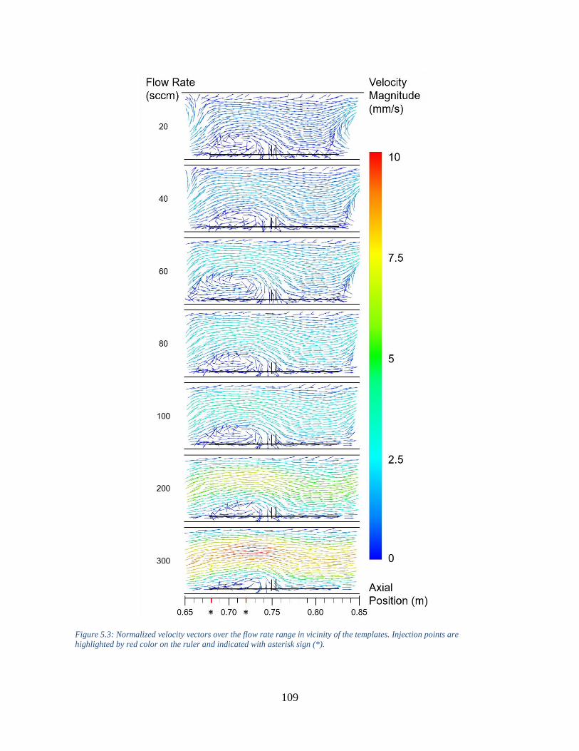
109
Figure 5.3: Normalized velocity vectors over the flow rate range in vicinity of the templates. Injection points are
highlighted by red color on the ruler and indicated with asterisk sign (*).
110
Recirculation center point and its area of effect can influence the residence time of the particles
reacting near the templates (Fogler 1986). The idea of using the residence time distribution
(RTD) in the analysis of chemical reactor performance, was first proposed by MacMullin and
Weber (MacMullin and Weber 1935). The concept did not appear to be used extensively until
early 1950s, when P. V. Danckwerts gave organizational structure to the subject of RTD by
defining most of the distributions of interest (Danckwerts 1953). By employing the same setup
for the analysis, it was hypothesized that this recirculation region can have a direct relation to the
residence time of ethylene particles. Residence time distribution of the particles can help in
explaining the experimental carbon mass deposition trend as a function of flow rate.
Particle tracking to find the residence time of particles
To further study the qualitatively observed recirculation effects, tracer particles with constant
molecular diameters (in the order of 10-10), and with density and specific heat of ethylene at
680°C are injected in cross sections 0.68 m and 0.72 m along the tube furnace (details of
injection procedure is explained in computational methods).
In 0.68 injection point the recirculation area is observed as a deadzone for the newly introduced
particles however in the second injection point (0.72 m), trajectories of the particles inside the
recirculation region are collected.
Figure 5.3a shows the peak mean residence time of the injected particles, which happens at 200
sccm inlet flow rate. After this peak, the mean residence time decreases as the flow rate is further
increased. To validate this peak, mean residence time at 400 sccm was numerically measured
(Res Time = 1430 s), which confirms that the peak residence time is at 200 sccm.
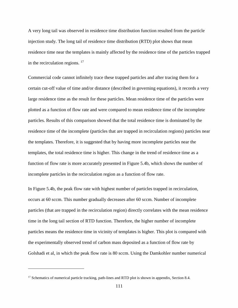
111
A very long tail was observed in residence time distribution function resulted from the particle
injection study. The long tail of residence time distribution (RTD) plot shows that mean
residence time near the templates is mainly affected by the residence time of the particles trapped
in the recirculation regions. 17
Commercial code cannot infinitely trace these trapped particles and after tracing them for a
certain cut-off value of time and/or distance (described in governing equations), it records a very
large residence time as the result for these particles. Mean residence time of the particles were
plotted as a function of flow rate and were compared to mean residence time of the incomplete
particles. Results of this comparison showed that the total residence time is dominated by the
residence time of the incomplete (particles that are trapped in recirculation regions) particles near
the templates. Therefore, it is suggested that by having more incomplete particles near the
templates, the total residence time is higher. This change in the trend of residence time as a
function of flow rate is more accurately presented in Figure 5.4b, which shows the number of
incomplete particles in the recirculation region as a function of flow rate.
In Figure 5.4b, the peak flow rate with highest number of particles trapped in recirculation,
occurs at 60 sccm. This number gradually decreases after 60 sccm. Number of incomplete
particles (that are trapped in the recirculation region) directly correlates with the mean residence
time in the long tail section of RTD function. Therefore, the higher number of incomplete
particles means the residence time in vicinity of templates is higher. This plot is compared with
the experimentally observed trend of carbon mass deposited as a function of flow rate by
Golshadi et al, in which the peak flow rate is 80 sccm. Using the Damkohler number numerical
17 Schematics of numerical particle tracking, path-lines and RTD plot is shown in appendix, Section 8.4.

112
value of residence time can be related to the conversion. Since, the reaction order is 1 and
reaction constant is available from literature (Becker and Hüttinger 1998; Albert and Luft 1999),
Damkohler number is only related to residence time or as it is stated here, the number of trapped
particles.
Having a relatively higher number of trapped particles will skew the residence time distribution
toward a higher value and therefore Damkohler number will increase. As a result, more reactants
can react near the templates and carbon mass deposition will increase.
Furthermore, during each physical run of TB-CVD process, traces of carbon residue was found
further downstream the tube furnace. This area coincides with a deadzone (recirculation) that is
numerically observed after the templates, further downstream the flow. Therefore, carbon
byproducts in ethylene reaction can diffuse through and deposit in this deadzone. The center-
point of this deadzone is located at 0.92 m along the axis on the bottom wall of tube furnace and
the effective radius is 0.05 m around the center-point.
Figure 5.4: Residence time of the particles trapped in recirculation region as a function of flow rate (a). Comparison
between the fractions of the particles trapped in recirculation region and mass deposition rate of carbon as a function of flow
rate (adapted from Golshadi et al.) (b).
Re
sid
en
ce T
ime
(s)
10
2 a)
0
0.1
0.2
0.3
0.4
0.5
0.6
0
0.05
0.1
0.15
0.2
0.25
0.3
0 100 200 300
Flow Rate (sccm)
b)
Ma
ss D
ep
ositio
n R
ate
(m
g/h
)
Fra
ctio
n o
f T
rap
pe
d P
art
icle
sΔ Golshadi et al.
Current approach0
5
10
15
20
25
30
0 100 200 300
Flow rate (sccm)
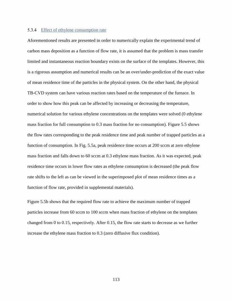
113
Effect of ethylene consumption rate
Aforementioned results are presented in order to numerically explain the experimental trend of
carbon mass deposition as a function of flow rate, it is assumed that the problem is mass transfer
limited and instantaneous reaction boundary exists on the surface of the templates. However, this
is a rigorous assumption and numerical results can be an over/under-prediction of the exact value
of mean residence time of the particles in the physical system. On the other hand, the physical
TB-CVD system can have various reaction rates based on the temperature of the furnace. In
order to show how this peak can be affected by increasing or decreasing the temperature,
numerical solution for various ethylene concentrations on the templates were solved (0 ethylene
mass fraction for full consumption to 0.3 mass fraction for no consumption). Figure 5.5 shows
the flow rates corresponding to the peak residence time and peak number of trapped particles as a
function of consumption. In Fig. 5.5a, peak residence time occurs at 200 sccm at zero ethylene
mass fraction and falls down to 60 sccm at 0.3 ethylene mass fraction. As it was expected, peak
residence time occurs in lower flow rates as ethylene consumption is decreased (the peak flow
rate shifts to the left as can be viewed in the superimposed plot of mean residence times as a
function of flow rate, provided in supplemental materials).
Figure 5.5b shows that the required flow rate to achieve the maximum number of trapped
particles increase from 60 sccm to 100 sccm when mass fraction of ethylene on the templates
changed from 0 to 0.15, respectively. After 0.15, the flow rate starts to decrease as we further
increase the ethylene mass fraction to 0.3 (zero diffusive flux condition).
114
Therefore, having less consumption rate near the templates results in more dominant viscous
effects on the overall flow pattern. Qualitative observations on contours of particle tracks also
confirms that in mass fractions of ethylene higher than 0.15 (less consumption), the area of effect
of the recirculation regions is dampened and does not exist in flow rates higher than 60 sccm.
Therefore, in the absence of recirculation regions, residence time of the injected particles is less
dependent on the long tail of RTD plot (i.e. the number of trapped particles), and will decrease as
the bulk velocity of the fluid continues to increase.
Conclusion
2D transient and 3D steady state, laminar, multi-species numerical models with instantaneous
reaction boundary condition (without modeling the reaction) are suggested to explain the
experimentally observed trend of carbon mass deposition as a function of time and inlet flow
rate. Steady state ethylene mass fractions achieved after 15 minutes of numerical time from
transient solution. This model suggests that diffusion of ethylene-helium mixture inside the
argon residing in our TB-CVD system can be a contributing factor to the ramp up time required
before the carbon mass deposition can linearly increase. In addition, 2D transient and 3D steady
Figure 5.5: Peak flow rate, corresponding to the maximum residence time of the particles (a), and to the maximum number of
trapped particles (b) as a function of Mass fraction.
0
50
100
150
200
250
0 0.1 0.2 0.3
Mass Fraction of Ethylene
Pe
ak F
low
Rate
(sccm
) a)
0
20
40
60
80
100
120
0 0.1 0.2 0.3Mass Fraction of Ethylene
Pe
ak F
low
Rate
(sccm
) b)

115
state models shown that the concentration of ethylene (reactant) in vicinity of templates, always
increases as a function of flow rate.
Discrete phase modeling (particle tracking) is employed on the more robust, 3D steady state
model, to explain the conversion rate which corresponds to the mean residence time of the
reactant particles, near the templates. Mean residence time was correlated with number of
particles trapped in recirculation region near the templates. Group particle injections showed that
the number of trapped particles and the residence time, both increased as a function of flow rate
until they reach to a certain flow rate (which depends on the consumption rate of ethylene and
area of effect of the recirculations), where they start to decrease by further increasing the flow
rate. These results are comparable to the experimentally observed trend of carbon mass deposited
on templates as a function of flow rate. This numerical model suggests that the curved shape of
the experimental results is caused by recirculation regions (deadzones) that appear in various
radius and strengths in vicinity of the templates.

116
Conclusion and Future Work

117
6 Conclusion and Future Work In the first phase of this study, various 3D and 2D models were developed to mimic the thermo-
fluid behavior in the TB-CVD processes used to manufacture CNTs. It was noticed that the
numerical modeling parameters affect thermo-fluid behavior inside the TB-CVD tube furnace.
Comparisons were made between each set of models and the most accurate model was chosen
for the next iteration of model comparison. Model M-4 was recommended as the most accurate
representation for this particular TB-CVD system. On the other hand, symmetric and fairly
constant temperature and buoyancy effects were observed in the middle of the tube furnace.
Velocity showed a direct relation with inlet flow rate, especially the axial velocity. But v and w
component were governed by buoyancy effects.
In the second phase of this study, previously recommended model was employed as 2D transient
and 3D steady state, laminar, multi-species numerical models with instantaneous reaction
boundary condition (without modeling the reaction) to explain the experimentally observed trend
of carbon mass deposition as a function of time and inlet flow rate. Steady state ethylene mass
fractions achieved after 15 minutes of numerical time from transient solution. This model
suggests that diffusion of ethylene-helium mixture inside the argon residing in our TB-CVD
system can be a contributing factor to the ramp up time required to achieve a linear carbon mass
deposition. Concentration gradient results shown that the concentration of ethylene (reactant) in
vicinity of templates, always increases as a function of flow rate.
Discrete phase modeling (particle tracking) is employed to explain the conversion rate which
corresponds to the mean residence time of the reactant particles, near the templates. Mean
residence time was correlated with number of particles trapped in recirculation region near the
templates. Group particle injections shown that the number of trapped particles and the residence

118
time increase as a function of flow rate until they reach to a certain flow rate (which depends on
the consumption rate of ethylene), where they start to decrease by further increasing the flow
rate. These results are comparable to the experimentally observed trend of carbon mass deposited
on templates as a function of flow rate. This numerical model suggests that the curved shape of
the experimental results is caused by recirculation regions (deadzones) that appear in various
radius and strengths in vicinity of the templates.
This work lays the groundwork for predicting the outcome of the TB-CVD process employed in
our lab to manufacture CNTs and related devices. Ultimately, the work will provide predictive
models to facilitate the efficient manufacture of carbon nanostructures from a variety of
templates for use in biomedical applications.
Future work
Based on the available literature and the current numerical work, following methods are
suggested to improve the accuracy of the predicted trend in comparison to the experimental
observations. Future models have the potential to represent various furnace conditions:
I. Conducting gas chromatography can provide the outlet concentration of ethylene for all
the flow rates tested during our carbon nanotube manufacturing TB-CVD process. This
method is promising in finding the exact value of ethylene consumption boundary
condition, required to model ethylene consumption on templates.
II. Reaction modeling needs to be performed, in order to compare the simplified model,
which is presented here, with a numerical model with no assumptions for reaction.
III. Smoke test and physical particle injection are also experimental alternatives to numerical
particle injection model.
119
7 References
A. Lautenschleger, A. Olenberg. 2015. “A Systematic CFD-Based Method to Investigate and
Optimise Novel Structured Packings.” Chemical Engineering Science 122.
doi:10.1016/j.ces.2014.09.040.
Albert, Jens, and Gerhard Luft. 1999. “Thermal Decomposition of Ethylene–comonomer
Mixtures under High Pressure.” AIChE Journal 45 (10): 2214–22.
doi:10.1002/aic.690451019.
Andrews, R., D. Jacques, A. M. Rao, F. Derbyshire, D. Qian, X. Fan, E. C. Dickey, and J. Chen.
1999. “Continuous Production of Aligned Carbon Nanotubes: A Step Closer to
Commercial Realization.” Chemical Physics Letters 303 (5–6): 467–74.
doi:10.1016/S0009-2614(99)00282-1.
ANSYS® FLUENT, 15.0.7, ANSYS, Inc.
Barone, Paul W., Seunghyun Baik, Daniel A. Heller, and Michael S. Strano. 2005. “Near-
Infrared Optical Sensors Based on Single-Walled Carbon Nanotubes.” Nature Materials
4 (1): 86–92. doi:10.1038/nmat1276.
Baughman, Ray H., Et Al, Ray H. Baughman, Anvar A. Zakhidov, and Walt A. De Heer. 2002 .
“Carbon Nanotubes—The Route Toward Applications.” Science, 787–92.
Becker, A., and K. J. Hüttinger. 1998. “Chemistry and Kinetics of Chemical Vapor Deposition of
pyrocarbon—II Pyrocarbon Deposition from Ethylene, Acetylene and 1,3-Butadiene in
the Low Temperature Regime.” Carbon 36 (3): 177–99. doi:10.1016/S0008-
6223(97)00175-9.
Bergles, A. E, and R. R Simonds. 1971. “Combined Forced and Free Convection for Laminar
Flow in Horizontal Tubes with Uniform Heat Flux.” International Journal of Heat and
Mass Transfer 14 (12): 1989–2000. doi:10.1016/0017-9310(71)90023-8.
Betzig, E., A. Lewis, A. Harootunian, M. Isaacson, and E. Kratschmer. 1986. “Near Field
Scanning Optical Microscopy (NSOM): Development and Biophysical Applications.”
Biophysical Journal 49 (1): 269–79. doi:10.1016/S0006-3495(86)83640-2.
Bianco, Alberto, Kostas Kostarelos, and Maurizio Prato. 2005. “Applications of Carbon
Nanotubes in Drug Delivery.” Current Opinion in Chemical Biology, Biopolymers /
Model systems, 9 (6): 674–79. doi:10.1016/j.cbpa.2005.10.005.

120
Bich, E., J. Millat, and E. Vogel. 1990. “The Viscosity and Thermal-Conductivity of Pure
Monatomic Gases from Their Normal Boiling-Point up to 5000-K in the Limit of Zero
Density And.” Journal of Physical and Chemical Reference Data 19 (6): 1289–1305.
Birakayala, Narayana, and Edward A Evans. 2002. “A Reduced Reaction Model for Carbon
CVD/CVI Processes.” Carbon 40 (5): 675–83. doi:10.1016/S0008-6223(01)00184-1.
Bockris, John O’M., White, Ralph E., Conway, Brian E. 1989. Modern Aspects of
Electrochemistry. Springer, volume 20, ISBN: 978-1-4684-8764-0.
Bowen, Ray M. 1976. “Part I - Theory of Mixtures.” In Continuum Physics, edited by A.
CEMAL ERINGEN, 1–127. Academic Press.
Chapman, Sydney, and T. G Cowling. 1970. “The Mathematical Theory of Non-Uniform Gases :
An Account of the Kinetic Theory of Viscosity, Thermal Conduction and Diffusion in
Gases.”
Chase, Malcom W. 1997. “Constants of Inorganic Substances. A Handbook. Revised and
Augmented Edition. By R. A. Lidin, L. L. Andreeva, and V. A. Molochko. Begell House,
Inc.: New York. 1996. 444 P. ISBN 1-56700-014-X.” Journal of Chemical &
Engineering Data 42 (1): 223–24. doi:10.1021/je960369x.
Che, G., B. B. Lakshmi, C. R. Martin, E. R. Fisher, and Rodney S. Ruoff. 1998. “Chemical
Vapor Deposition Based Synthesis of Carbon Nanotubes and Nanofibers Using a
Template Method.” Chemistry of Materials 10 (1): 260–67. doi:10.1021/cm970412f.
“Chemical Vapour Deposition Systems Design.” 2010. In Chemical Vapour Deposition, 73–128.
Engineering Materials and Processes. Springer London.
Cheng, W. T., H. C. Li, and C. N. Huang. 2008. “Simulation and Optimization of Silicon
Thermal CVD through CFD Integrating Taguchi Method.” Chemical Engineering
Journal 137 (3): 603–13. doi:10.1016/j.cej.2007.05.042.
Chiu, W. K. S., C. J. Richards, and Y. Jaluria. 2000. “Flow Structure and Heat Transfer in a
Horizontal Converging Channel Heated from below.” Physics of Fluids 12 (8): 2128–36.
doi:10.1063/1.870458.
Choudhury, D., and S. V. Patankar. 1988. “Combined Forced and Free Laminar Convection in
the Entrance Region of an Inclined Isothermal Tube.” Journal of Heat Transfer 110 (4a):
901–9. doi:10.1115/1.3250591.
121
Cho, Wondong, Mark Schulz, and Vesselin Shanov. 2013. “Kinetics of Growing Centimeter
Long Carbon Nanotube Arrays.” In Syntheses and Applications of Carbon Nanotubes and
Their Composites, edited by Satoru Suzuki. InTech.
Choy, K. L. 2003. “Chemical Vapour Deposition of Coatings.” Progress in Materials Science 48
(2): 57–170. doi:10.1016/S0079-6425(01)00009-3.
Ciambelli, P., L. Arurault, M. Sarno, S. Fontorbes, C. Leone, L. Datas, D. Sannino, P.
Lenormand, and S. Le Blond Du Plouy. 2011. “Controlled Growth of CNT in
Mesoporous AAO through Optimized Conditions for Membrane Preparation and CVD
Operation.” Nanotechnology 22 (26): 265613. doi:10.1088/0957-4484/22/26/265613.
Ciambelli, P., D. Sannino, M. Sarno, A. Fonseca, and J. B. Nagy. 2004. “Hydrocarbon
Decomposition in Alumina Membrane: An Effective Way to Produce Carbon Nanotubes
Bundles.” Journal of Nanoscience and Nanotechnology 4 (7): 779–87.
Coltrin, Michael E., Robert J. Kee, and James A. Miller. 1986. “A Mathematical Model of
Silicon Chemical Vapor Deposition Further Refinements and the Effects of Thermal
Diffusion.” Journal of The Electrochemical Society 133 (6): 1206–13.
doi:10.1149/1.2108820.
Dai, Hongjie. 2002. “Carbon Nanotubes: Opportunities and Challenges.” Surface Science 500
(1–3): 218–41. doi:10.1016/S0039-6028(01)01558-8.
Danckwerts, P. V. 1953. “Continuous Flow Systems.” Chemical Engineering Science 2 (1): 1–
13. doi:10.1016/0009-2509(53)80001-1.
Danckwerts, P. V., and Arvo Lannus. 1970. “Gas‐Liquid Reactions.” Journal of The
Electrochemical Society 117 (10): 369C – 370C. doi:10.1149/1.2407312.
De la Zerda, Adam, Cristina Zavaleta, Shay Keren, Srikant Vaithilingam, Sunil Bodapati,
Zhuang Liu, Jelena Levi, et al. 2008. “Carbon Nanotubes as Photoacoustic Molecular
Imaging Agents in Living Mice.” Nature Nanotechnology 3 (9): 557–62.
doi:10.1038/nnano.2008.231.
De Volder, M. F. L., S. H. Tawfick, R. H. Baughman, and A. J. Hart. 2013. “Carbon Nanotubes:
Present and Future Commercial Applications.” Science 339 (6119): 535–39.
doi:10.1126/science.1222453.
Dixiao, Bao. 2012. Transport of Multi-Walled Carbon Nanotubes in Saturated Porous Media.

122
Endo, Hajime, Kazunori Kuwana, Kozo Saito, Dali Qian, Rodney Andrews, and Eric A. Grulke.
2004. “CFD Prediction of Carbon Nanotube Production Rate in a CVD Reactor.”
Chemical Physics Letters 387 (4–6): 307–11. doi:10.1016/j.cplett.2004.01.124.
F. C. Eversteyn, P. J. W. Severin. 1970. “A Stagnant Layer Model for the Epitaxial Growth of
Silicon from Silane in a Horizontal Reactor.” Journal of The Electrochemical Society - J
ELECTROCHEM SOC 117 (7). doi:10.1149/1.2407685.
Fleischmann, M., P. J. Hendra, and A. J. McQuillan. 1974. “Raman Spectra of Pyridine
Adsorbed at a Silver Electrode.” Chemical Physics Letters 26 (2): 163–66.
doi:10.1016/0009-2614(74)85388-1.
Fleisher, R. L., P. B. Price, and R. M. Walker. 1975. Nuclear Tracks in Solids: Principles and
Applications.
Fogler, H. Scott. 1986. Elements of Chemical Reaction Engineering. Prentice-Hall.
Fotiadis, Dimitrios I., and Klavs F. Jensen. 1990. “Thermophoresis of Solid Particles in
Horizontal Chemical Vapor Deposition Reactors.” Journal of Crystal Growth 102 (4):
743–61. doi:10.1016/0022-0248(90)90838-C.
Giling, L. J. 1982. “Gas Flow Patterns in Horizontal Epitaxial Reactor Cells Observed by
Interference Holography.” Journal of The Electrochemical Society 129 (3): 634–44.
doi:10.1149/1.2123939.
Golshadi, Masoud, Jessica Maita, David Lanza, Marco Zeiger, Volker Presser, and Michael G.
Schrlau. 2014. “Effects of Synthesis Parameters on Carbon Nanotubes Manufactured by
Template-Based Chemical Vapor Deposition.” Carbon 80 (December): 28–39.
doi:10.1016/j.carbon.2014.08.008.
Guermond, J. L., P. Minev, and Jie Shen. 2006. “An Overview of Projection Methods for
Incompressible Flows.” Computer Methods in Applied Mechanics and Engineering 195
(44–47): 6011–45. doi:10.1016/j.cma.2005.10.010.
Haar, D. Ter. 1954. “Molecular Theory of Gases and Liquids. Joseph O. Hirschfelder, Charles F.
Curtiss, and R. Byron Bird. Wiley, New York; Chapman & Hall, London, 1954. Xxvi +
1219 Pp. Illus. $20.” Science 120 (3131): 1097–1097.
doi:10.1126/science.120.3131.1097.

123
Harris, Peter J. F. 2009. Carbon Nanotube Science : Synthesis, Properties and Applications.
Cambridge, GBR: Cambridge University Press.
http://site.ebrary.com/lib/alltitles/docDetail.action?docID=10297145.
He, Delong, Hao Li, and Jinbo Bai. 2011. “Experimental and Numerical Investigation of the
Position-Dependent Growth of Carbon Nanotube–alumina Microparticle Hybrid
Structures in a Horizontal CVD Reactor.” Carbon 49 (15): 5359–72.
doi:10.1016/j.carbon.2011.08.003.
H. K. (Henk Kaarle) Versteeg, W. (Weeratunge) Malalasekera. n.d. “An Introduction to
Computational Fluid Dynamics : The Finite Volume Method / H. K. Versteeg and W.
Malalasekera.” SERBIULA (sistema Librum 2.0).
Holland, P. M., B. E. Eaton, and H. J. M. Hanley. 1983. “A Correlation of the Viscosity and
Thermal Conductivity Data of Gaseous and Liquid Ethylene.” Journal of Physical and
Chemical Reference Data 12 (4): 917–32. doi:10.1063/1.555701.
Hulteen, John C., and Charles R. Martin. 1997. “A General Template-Based Method for the
Preparation of Nanomaterials.” Journal of Materials Chemistry 7 (7): 1075–87.
doi:10.1039/A700027H.
Ibrahim, John, and Samuel Paolucci. 2011. “Transient Solution of Chemical Vapor
Infiltration/deposition in a Reactor.” Carbon 49 (3): 915–30.
doi:10.1016/j.carbon.2010.11.002.
I. Guillén, C. Treviño. 2014. “Unsteady Laminar Mixed Convection Heat Transfer from a
Horizontal Isothermal Cylinder in Contra-Flow: Buoyancy and Wall Proximity Effects on
the Flow Response and Wake Structure.” Experimental Thermal and Fluid Science 52:
30–46. doi:10.1016/j.expthermflusci.2013.08.019.
Iijima, Sumio. 1991. “Helical Microtubules of Graphitic Carbon.” Nature 354 (6348): 56.
Iijima, Sumio, and Toshinari Ichihashi. 1993. “Single-Shell Carbon Nanotubes of 1-Nm
Diameter.” Nature 363 (6430): 603–5. doi:10.1038/363603a0.
Ingham, Dr D. B., and Dr J. H. Merkin. 1981. “Unsteady Mixed Convection from an Isothermal
Circular Cylinder.” Acta Mechanica 38 (1-2): 55–69. doi:10.1007/BF01351462.
Jain, P. C., and B. L. Lohar. 1979. “Unsteady Mixed Convection Heat Transfer from a
Horizontal Circular Cylinder.” Journal of Heat Transfer 101 (1): 126–31.
doi:10.1115/1.3450902.
124
Jianmin Ding, Dimitri Gidaspow. 2004. “A Bubbling Fluidization Model Using Kinetic Theory
of Granular Flow.” AIChE Journal 36 (4): 523–38. doi:10.1002/aic.690360404.
Johnson, G., M. Massoudi, and K. R. Rajagopal. 1991. “Flow of a Fluid—solid Mixture between
Flat Plates.” Chemical Engineering Science 46 (7): 1713–23. doi: 10.1016/0009-
2509(91)87018-8.
Jones, Anthony C., and Michael L. Hitchman. 2008 “Chemical Vapour Deposition - Precursors,
Processes and Applications.” Royal Society of Chemistry. ISBN: 978-0-85404-465-8. doi:
10.1039/9781847558794.
Jones, J. E. 1924. “On the Determination of Molecular Fields. II. From the Equation of State of a
Gas.” Proceedings of the Royal Society of London A: Mathematical, Physical and
Engineering Sciences 106 (738): 463–77. doi:10.1098/rspa.1924.0082.
Joseph, D. D., T. S. Lundgren, R. Jackson, and D. A. Saville. 1990. “Ensemble Averaged and
Mixture Theory Equations for Incompressible Fluid—particle Suspensions.”
International Journal of Multiphase Flow 16 (1): 35–42. doi: 10.1016/0301-
9322(90)90035-H.
Joseph O. Hirschfelder, Charles F. Curtiss. 1955. “Molecular Theory of Gases and Liquids / J.O.
Hirschfelder, C.F. Curtiss, R. Byron Bird.”
Kam, Nadine Wong Shi, Michael O’Connell, Jeffrey A. Wisdom, and Hongjie Dai. 2005.
“Carbon Nanotubes as Multifunctional Biological Transporters and near-Infrared Agents
for Selective Cancer Cell Destruction.” Proceedings of the National Academy of Sciences
of the United States of America 102 (33): 11600–605. doi:10.1073/pnas.0502680102.
Kleijn, Chris R. 2000. “Computational Modeling of Transport Phenomena and Detailed
Chemistry in Chemical Vapor Deposition – a Benchmark Solution.” Thin Solid Films 365
(2): 294–306. doi:10.1016/S0040-6090(99)01060-3.
Koronaki, E. D, H. H Liakos, M. A Founti, and N. C Markatos. 2001. “Numerical Study of
Turbulent Diesel Flow in a Pipe with Sudden Expansion.” Applied Mathematical
Modelling 25 (4): 319–33. doi: 10.1016/S0307-904X(00)00055-X.
Kuo, Kenneth K. 1986. Principles of Combustion. Wiley.
Kuwana, Kazunori, Tianxiang Li, and Kozo Saito. 2006. “Gas-Phase Reactions during CVD
Synthesis of Carbon Nanotubes: Insights via Numerical Experiments.” Chemical
Engineering Science 61 (20): 6718–26. doi:10.1016/j.ces.2006.07.006.
125
Kuwana, Kazunori, and Kozo Saito. 2005. “Modeling CVD Synthesis of Carbon Nanotubes:
Nanoparticle Formation from Ferrocene.” Carbon 43 (10): 2088–95.
doi:10.1016/j.carbon.2005.03.016.
Kyotani, Takashi, Li-fu Tsai, and Akira Tomita. 1995. “Formation of Ultrafine Carbon Tubes by
Using an Anodic Aluminum Oxide Film as a Template.” Chemistry of Materials 7 (8):
1427–28. doi:10.1021/cm00056a001.
Lacerda, Lara, Simona Raffa, Maurizio Prato, Alberto Bianco, and Kostas Kostarelos. 2007.
“Cell-Penetrating CNTs for Delivery of Therapeutics.” Nano Today 2 (6): 38–43.
doi:10.1016/S1748-0132(07)70172-X.
Lax, P. D., and R. D. Richtmyer. 1956. “Survey of the Stability of Linear Finite Difference
Equations.” Communications on Pure and Applied Mathematics 9 (2): 267–93.
doi:10.1002/cpa.3160090206.
Levenspiel, Octave. 1999. “Chemical Reaction Engineering.” Industrial & Engineering
Chemistry Research 38 (11): 4140–43. doi:10.1021/ie990488g.
Li, Juntao, Wei Lei, Xiaobing Zhang, Baoping Wang, and Long Ba. 2004. “Field Emission of
Vertically-Aligned Carbon Nanotube Arrays Grown on Porous Silicon Substrate.” Solid-
State Electronics 48 (12): 2147–51. doi:10.1016/j.sse.2004.06.011.
Li, Yusong, Yonggang Wang, Kurt D. Pennell, and Linda M. Abriola. 2008. “Investigation of
the Transport and Deposition of Fullerene (C60) Nanoparticles in Quartz Sands under
Varying Flow Conditions.” Environmental Science & Technology 42 (19): 7174–80.
doi:10.1021/es801305y.
Lord, H. A. 1987. “Convective Transport in Silicon Epitaxial Deposition in a Barrel Reactor.”
Journal of The Electrochemical Society 134 (5): 1227–35. doi:10.1149/1.2100647.
L. V.Radushkevich, V. M. Lukyanovich. 1952. “About the Structure of Carbon Formed by
Thermal Decomposition of Carbon Monoxide on Iron Substrate.” Zurn. Fisic. Chim. 26:
88–95.
MacMullin, R. B., and M. Weber, Jr. 1935. “The Theory of Short-Circuiting in Continuous-Flow
Mixing Vessels in Series and Kinetics of Chemical Reactions in Such Systems.” Trans.
Am. Inst. Chem. Eng. 31 (409).
Manninen, M, V Taivassalo, and S Kallio. 1996. “On the Mixture Model for Multiphase Flow.”
VTT Publications 288, Technical Research Centre of Finland.

126
Martin, C. R. 1994. “Nanomaterials: A Membrane-Based Synthetic Approach.” Science (New
York, N.Y.) 266 (5193): 1961–66. doi:10.1126/science.266.5193.1961.
Mazumder, Sandip. 2006. “Critical Assessment of the Stability and Convergence of the
Equations of Multi-Component Diffusion.” Journal of Computational Physics 212 (2):
383–92. doi:10.1016/j.jcp.2005.07.018.
Miller, S. A., V. Y. Young, and C. R. Martin. 2001. “Electroosmotic Flow in Template-Prepared
Carbon Nanotube Membranes.” Journal of the American Chemical Society 123 (49):
12335–42. doi:10.1021/ja011926p.
Mirramezani, Mehran, Hamid Reza Mirdamadi, and Mostafa Ghayour. 2013. “Innovative
Coupled Fluid–structure Interaction Model for Carbon Nano-Tubes Conveying Fluid by
Considering the Size Effects of Nano-Flow and Nano-Structure.” Computational
Materials Science 77 (September): 161–71. doi:10.1016/j.commatsci.2013.04.047.
Mishra, Pratyush, and Nishith Verma. 2012. “A CFD Study on a Vertical Chemical Vapor
Deposition Reactor for Growing Carbon Nanofibers.” Chemical Engineering Research
and Design 90 (12): 2293–2301. doi:10.1016/j.cherd.2012.05.006.
Mosteller, Frederick, and R. A. Fisher. 1948. “Questions and Answers.” The American
Statistician 2 (5): 30–31. doi:10.2307/2681650.
Narasimha, M., Matthew Brennan, and P. N. Holtham. 2007. “A Review of CFD Modelling for
Performance Predictions of Hydrocyclone.” Engineering Applications of Computational
Fluid Mechanics 1 (2): 109–25. doi:10.1080/19942060.2007.11015186.
Newell, P. H., and A. E. Bergles. 1970. “Analysis of Combined Free and Forced Convection for
Fully Developed Laminar Flow in Horizontal Tubes.” Journal of Heat Transfer 92 (1):
83. doi:10.1115/1.3449650.
Oberlin, A., M. Endo, and T. Koyama. 1976. “Filamentous Growth of Carbon through Benzene
Decomposition.” Journal of Crystal Growth 32 (3): 335–49. doi:10.1016/0022-
0248(76)90115-9.
Ong, Yit Thai, Abdul Latif Ahmad, Sharif Hussein Sharif Zein, and Soon Huat Tan. 2010. “A
Review on Carbon Nanotubes in an Environmental Protection and Green Engineering
Perspective.” Brazilian Journal of Chemical Engineering 27 (2): 227–42.
doi:10.1590/S0104-66322010000200002.

127
Patankar, S. V., S. Ramadhyani, and E. M. Sparrow. 1978. “Effect of Circumferentially
Nonuniform Heating on Laminar Combined Convection in a Horizontal Tube.” Journal
of Heat Transfer 100 (1): 63. doi:10.1115/1.3450505.
Patolsky, Fernando, Gengfeng Zheng, and Charles M Lieber. 2006. “Fabrication of Silicon
Nanowire Devices for Ultrasensitive, Label-Free, Real-Time Detection of Biological and
Chemical Species.” Nature Protocols 1 (4): 1711–24. doi:10.1038/nprot.2006.227.
Poling, Bruce E. 2001. The Properties of Gases and Liquids. 5th ed. New York: McGraw-Hill.
Rhie, C. M., and W. L. Chow. 1983. “Numerical Study of the Turbulent Flow Past an Airfoil
with Trailing Edge Separation.” AIAA Journal 21 (November): 1525–32.
doi:10.2514/3.8284.
Riley, H. L. 1947. “Amorphous Carbon and Graphite.” Quarterly Reviews, Chemical Society 1
(1): 59–72. doi:10.1039/QR9470100059.
Robinson, J. A., E. S. Snow, and F. K. Perkins. 2007. “Improved Chemical Detection Using
Single-Walled Carbon Nanotube Network Capacitors.” Sensors and Actuators A:
Physical 135 (2): 309–14. doi:10.1016/j.sna.2006.07.027.
Rogers, G. F. C., and Yon R. Mayhew. 1994. Thermodynamic and Transport Properties of
Fluids: S. I. Units. 5th Edition edition. Oxford: Wiley-Blackwell.
SA Morsi, AJ Alexander. 1972. “An Investigation of Particle Trajectories in Two-Phase Flow
Systems.” Journal of Fluid Mechanics 55 (02): 193–208.
doi:10.1017/S0022112072001806.
Santra, Tuhin Subhra, and Fan Gang Tseng. 2014. “Micro/Nanofluidic Devices for Single Cell
Analysis.” Micromachines 5 (2): 154–57. doi:10.3390/mi5020154.
Sarno, Maria, Diana Sannino, Caterina Leone, and Paolo Ciambelli. 2012. “CNTs Tuning and
Vertical Alignment in Anodic Aluminium Oxide Membrane.” Journal of Natural Gas
Chemistry 21 (6): 639–46. doi:10.1016/S1003-9953(11)60413-1.
Schiller, L., and Z. Naumann. 1935. “A Drag Coefficient Correlation.” Ver. Deutsch. Ing., 77–
318.
Schrlau, Michael G., Erica M. Falls, Barry L. Ziober, and Haim H. Bau. 2008. “Carbon
Nanopipettes for Cell Probes and Intracellular Injection.” Nanotechnology 19 (1):
015101. doi:10.1088/0957-4484/19/01/015101.

128
Shannon, R. L., and C. A. Depew. 1968. “Combined Free and Forced Laminar Convection in a
Horizontal Tube With Uniform Heat Flux.” Journal of Heat Transfer 90 (3): 353–57.
doi:10.1115/1.3597516.
Shi, Bao-Xian, Yu Wang, Tin-Lun Lam, Wei-Hua Huang, Kai Zhang, Yun-Chung Leung, and
Helen L. W. Chan. 2010. “Release Monitoring of Single Cells on a Microfluidic Device
Coupled with Fluorescence Microscopy and Electrochemistry.” Biomicrofluidics 4 (4):
043009. doi:10.1063/1.3491470.
Singhal, Riju, Zulfiya Orynbayeva, Ramalingam Venkat Kalyana Sundaram, Jun Jie Niu, Sayan
Bhattacharyya, Elina A. Vitol, Michael G. Schrlau, Elisabeth S. Papazoglou, Gary
Friedman, and Yury Gogotsi. 2011. “Multifunctional Carbon-Nanotube Cellular
Endoscopes.” Nature Nanotechnology 6 (1): 57–64. doi:10.1038/nnano.2010.241.
Sornek, Rafal J., Ritsu Dobashi, and Toshisuke Hirano. 2000. “Effect of Turbulence on
Vaporization, Mixing, and Combustion of Liquid-Fuel Sprays.” Combustion and Flame
120 (4): 479–91. doi:10.1016/S0010-2180(99)00105-4.
Stouffer, S. A., E. A. Suchman, A. E. Devinney, S. A. Star, and R. M. Jr. Williams. 1949. “The
American Soldier: Adjustment during Army Life. Volume I.” Journal of the American
Medical Association 140 (14): 1189–1189. doi:10.1001/jama.1949.02900490055028.
Taylor, Ross, and R Krishna. 1993. Multicomponent Mass Transfer. New York: Wiley.
Tesner, P. A., and S. V. Shurupov. 1994. “Some Physico-Chemical Parameters of Soot
Formation during Pyrolysis of Methane and Methane-Acetylene and Methane-Benzene
Mixtures.” Symposium (International) on Combustion 25 (1): 653–59.
doi:10.1016/S0082-0784(06)80697-1.
Thess, Andreas, Roland Lee, Pavel Nikolaev, and Hongjie Dai. 1996. “Crystalline Ropes of
Metallic Carbon Nanotubes.” Science 273 (5274): 483.
Todd, Randy, and David H. Margolin. 2002. “Challenges of Single-Cell Diagnostics: Analysis of
Gene Expression.” Trends in Molecular Medicine 8 (6): 254–57.
Vahedein, Yashar Seyed, and Michael G. Schrlau. 2015. “Numerical Model of Template-Based
Chemical Vapor Deposition Processes to Manufacture Carbon Nanotubes for Biological
Devices,” July, V001T03A005. doi:10.1115/ICNMM2015-48520.

129
Van Opdorp, C., and M. R. Leys. 1987. “On the Factors Impairing the Compositional Transition
Abruptness in Heterojunctions Grown by Vapour-Phase Epitaxy.” Journal of Crystal
Growth 84 (2): 271–88. doi:10.1016/0022-0248(87)90142-4.
Visser, E. P., C. R. Kleijn, C. A. M. Govers, C. J. Hoogendoorn, and L. J. Giling. 1989. “Return
Flows in Horizontal MOCVD Reactors Studied with the Use of TiO2 Particle Injection
and Numerical Calculations.” Journal of Crystal Growth 94 (4): 929–46.
doi:10.1016/0022-0248(89)90127-9.
Wangard III, William, David S. Dandy, and Brian J. Miller. 2001. “A Numerically Stable
Method for Integration of the Multicomponent Species Diffusion Equations.” Journal of
Computational Physics 174 (1): 460–72. doi:10.1006/jcph.2001.6930.
Wang, C. Y. 1989. “Effect of Non-Well-Mixed Compartment and Bulk Flow on Diffusion
through a Pore.” Mathematical Biosciences 95 (1): 99–109.
Weihua, Huang, H. U. Shen, Pang Daiwen, Wang Zongli, and Cheng Jieke. 2000. “Monitoring
the secretion from single cells with temporal and spatial resolution, Monitoring the
secretion from single cells with temporal and spatial resolution.” Chinese Science
Bulletin 45 (4): 289–95.
Xiao, Jinsheng, Liang Tong, Caihua Deng, Pierre Bénard, and Richard Chahine. 2010.
“Simulation of Heat and Mass Transfer in Activated Carbon Tank for Hydrogen
Storage.” International Journal of Hydrogen Energy 35 (15): 8106–16.
doi:10.1016/j.ijhydene.2010.01.021.
Yao, Kuan-Mu, Mohammad T. Habibian, and Charles R. O’Melia. 1971. “Water and Waste
Water Filtration. Concepts and Applications.” Environmental Science & Technology 5
(11): 1105–12. doi:10.1021/es60058a005.
Ye, Y., C. C. Ahn, C. Witham, B. Fultz, J. Liu, A. G. Rinzler, D. Colbert, K. A. Smith, and R. E.
Smalley. 1999. “Hydrogen Adsorption and Cohesive Energy of Single-Walled Carbon
Nanotubes.” Applied Physics Letters 74 (16): 2307–9. doi:10.1063/1.123833.
Yun, Kwang-Seok, and Euisik Yoon. 2005. “Micro/Nanofluidic Device for Single-Cell-Based
Assay.” Biomedical Microdevices 7 (1): 35–40. doi:http://dx.doi.org/10.1007/s10544-
005-6169-5.

130
Yusong Li, Yonggang Wang. 2008. “Investigation of the Transport and Deposition of Fullerene
(C60) Nanoparticles in Quartz Sands under Varying Flow Conditions.” Environmental
Science & Technology 42 (19): 7174–80. doi:10.1021/es801305y.
Zhang, Mei, and Jian Li. 2009. “Carbon Nanotube in Different Shapes.” Materials Today 12 (6):
12–18. doi:10.1016/S1369-7021(09)70176-2.
Zheng, Xin Ting, and Chang Ming Li. 2012. “Single Cell Analysis at the Nanoscale.” Chemical
Society Reviews 41 (6): 2061–71. doi:10.1039/C1CS15265C.
Zhou, Jie, and Colin A. Wolden. 2003. “Modeling and Measurement of Film Deposition in a
One-Dimensional Hot-Wire CVD System.” Thin Solid Films, Proceedings of the Second
International Conference on Cat-CVD (Hot Wire CVD) Process, 430 (1–2): 28–32.
doi:10.1016/S0040-6090(03)00126-3.

131
Appendix

132
8 Appendix
Governing equations and two phase model
General Navier-Stokes equation:
∂
∂t∫ ρφdV
V+ ∫ ρφV⃗⃗ ∙ dA
A= ∮ Γ∇φ ∙ dA
A+ ∮ SφdV
V (8.1)
In Equation 9.1, 𝜌 is density, 𝑉 is control volume, 𝐴 is contact area, 𝑡 is time and 𝜑 can be
replaced by intensive properties. The terms on the left are representing unsteady and convection
parts of the continuity equation. Two terms on the right exist when diffusion and/or generation
due to reaction are available in the system. Conservation equations are solved in two forms in
this work: single-phase (model with Ethylene as the inlet gas, referred herein as Model 1), and
multi-phase (for the model with ethylene and helium mixture as the inlet gas – referred herein as
Model 2). Interspecies diffusion in mixture flow is neglected since the mixture is considered to
be homogenous. The differential form:
𝜕𝜌
𝜕𝑡+ ∇ ∙ (𝜌�̅�) = 𝑆𝑚 (8.1)
𝑆𝑚 is the amount of mass that is generated, which in this case is equal to zero. Since the steady
state solution will be employed in this work, 𝜕𝜌
𝜕𝑡 and further mentioned derivatives with respect to
time will be equal to zero. Also �̅� is equal to mass averaged velocity:
�̅�𝑚 =∑ 𝛼𝑘𝜌𝑘�̅�𝑘
𝑛𝑘=1
𝜌𝑚 (8.2)
𝜌𝑚 = ∑ 𝛼𝑘𝜌𝑘𝑛𝑘=1 (8.3)
𝛼𝑘 is mass fraction of phase k. General form of momentum conservation is described by:

133
𝜕
𝜕𝑡(𝜌�̅�) + ∇ ∙ (𝜌�̅��̅�) = −∇𝑝 + ∇ ∙ (𝜏̅) + 𝜌�̅� + �̅� (8.4)
In which 𝜏̅ is the stress tensor and is given by:
𝜏̅ = 𝜇 [(∇�̅� + ∇v̅𝑇) −2
3∇ ∙ �̅�𝐼] (8.5)
The effect of volume dilation can be viewed in the right hand side of the Equation 8.6 (𝐼 is unit
tensor). When rewriting this equation for mixture, it will evolve to this condition:
𝜕
𝜕𝑡(𝜌𝑚�̅�𝑚) + ∇ ∙ (𝜌𝑚�̅�𝑚�̅�𝑚) = −∇𝑝 + ∇ ∙ (𝜏�̅�) + 𝜌𝑚�̅� + �̅� + ∇ ∙ (∑ 𝛼𝑘𝜌𝑘�̅�𝑑𝑟,𝑘�̅�𝑑𝑟,𝑘
𝑛𝑘=1 ) (8.6)
Here, n is number of phases and each parameter with m index indicates the mixture
specifications. �̅�𝑑𝑟,𝑘 is the drift velocity of the secondary phase k. Therfore:
�̅�𝑑𝑟,𝑘 = �̅�𝑘 − �̅�𝑚 (8.7)
The energy equation in integral form is:
𝜕
𝜕𝑡∫𝜌 (𝑒 +
1
2�̅�2) 𝑑𝑉 = −∮𝜌 (𝑒 +
1
2�̅�2) �̅� ∙ 𝑑𝐴 + ∫ �̅� ∙ 𝑓𝑑𝑉
𝑉+ ∮(�̅�𝜏̅)𝑑𝐴 − ∮𝑞𝑑𝐴 (8.8)
The left side of Equation 8.8 shows the rate of change for kinetic and internal energy (e is fluid
specific internal energy). The right side of Equation 8.8 from left to right is: a) the net inflow of
kinetic and thermal energy; b) work done by body forces (𝑓 is the body force density); c) work
done by stress tensor; and d) net heat flow (𝑞 is the amount of added heat). By further
simplification and conversion into differential form, the energy equation can be represented as:
𝜕
𝜕𝑡(𝜌𝐸) + ∇(�̅�(𝜌𝐸 + 𝑃)) = ∇ ∙ (𝑘𝑒𝑓𝑓∇𝑇 − ∑ ℎ𝑗𝐽�̅� + (𝜏�̅�𝑓𝑓 ∙ �̅�)𝑗 ) + 𝑆ℎ (8.9)

134
Here, 𝑘𝑒𝑓𝑓 is the effective conductivity, 𝐽�̅� is the Diffusion flux of species 𝑗. In the paranthesis
energy transferred by conduction, species diffusion, and viscous dissipation are shown
respectively. 𝑆ℎ is any generated energy such as from chemical reactions and so on. For the
mixture 𝜌, �̅�, 𝐸 will be replaced by 𝛼𝑘𝜌𝑘 , 𝛼𝑘�̅�𝑘, 𝛼𝑘𝐸𝑘.
The Mixture model (Model 2) (Manninen, Taivassalo, and Kallio 1996) is a valid substitute for
the full Eulerian multiphase model (Jianmin Ding 2004), Others have reported the Mixture
model performs as well as a full multiphase model but is more simple and saves computational
time because it only requires solving a smaller number of variables (Narasimha, Brennan, and
Holtham 2007). A homogeneous flow within the mixture model is applicable when the phases
are strongly coupled in drag-dominated flow and their velocities equalize over short spatial
length scales (Joseph et al. 1990; Johnson, Massoudi, and Rajagopal 1991; Bowen 1976). Since
the mixture model is used here, the pressure-based solver should be employed because the
Mixture model is not compatible with density-based solvers. Slip (relative) velocity is the
relative velocity between two or more species in a mixture model calculated by (Manninen,
Taivassalo, and Kallio 1996) is given below:
�̅�𝑝𝑞 =𝜏𝑝
𝑓𝑑𝑟𝑎𝑔
(𝜌𝑝−𝜌𝑚)
𝜌𝑝�̅� (8.10)
In which 𝜏𝑝 is particle relaxation time:
𝜏𝑝 =𝜌𝑝𝑑𝑝
2
18𝜇𝑞 (8.11)

135
Here, d is the diameter of the particles of secondary phase p and �̅� is the secondary-phase
acceleration of the particles. The default drag function, 𝑓𝑑𝑟𝑎𝑔, is taken from Schiller and
Naumann (Schiller and Naumann 1935):
𝑓𝑑𝑟𝑎𝑔 = {1 + 0.15𝑅𝑒0.687 𝑅𝑒 ≤ 10000.0183𝑅𝑒 𝑅𝑒 > 1000
(8.12)
Acceleration is given by �̅�:
�̅� = �̅� − (�̅�𝑚 ∙ ∇)�̅�𝑚 −𝜕�̅�𝑚
𝜕𝑡 (8.13)
The pressure-based method employs a set of equations known as projection method equations
(Guermond, Minev, and Shen 2006). Since the flow is mixed flow (not Eulerian) and
compressible, the coupled form of this solver method is applicable. The coupled algorithm solves
the momentum and pressure-based continuity equations together. The full implicit coupling is
achieved through an implicit discretization of pressure gradient terms in the momentum
equations, and an implicit discretization of the face mass flux, including the Rhie-Chow pressure
dissipation terms (Rhie and Chow 1983). Coupled AMG solver is used to solve linear transport
equations using implicit discretization from a coupled pressure-based scheme.
Initializing the simulation (Stefen-Maxwell model)
It is important to have a robust strategy to initialize a complex CFD problem. In order to
initialize this problem, which involves mixed convection, multi-species concentration (Maxwell
multi-species theorem) and recirculations, the following strategy is suggested after testing its
viability:

136
1- Initialize Stephen-Maxwell equation with zero ethylene and zero helium concentration.
This means that only the argon exists in the tube.
2- Run a steady state solution with only argon entering the tube to obtain the steady state
flow condition for argon, which is residing in the tube furnace at the start of the CVD
process.
3- Run a transient solution for 1 s of physical time with the following gas composition:
30/70 (vol%/vol%) ethylene/helium gas mixture at the inlet. This gas is entering to the
tube furnace while the boundary condition on the templates is constant 0 and 25 Vol%
ethylene concentration.
4- Calculate the steady state solution for the boundaries mentioned in number 3 in a coupled
solver with second order conservation equations.
Suggested descriptive statistical analysis
Suggested statistical approach for analyzing significance in non-repeating data sets
The large number of points in each analyzed cross section makes the interpretation of data more
and more qualitative. In the majority of CFD based works, it was noticed that the data analysis
was conducted with a qualitative observation based on resulted contour plots. Another common
method used to analyze the data is non-dimensionalized numbers to represent the features of the
flow that are being inspected. This method is reliable when the goal is analyzing the general
features of the flow (such as effects from momentum and viscosity in Reynolds number),
however, when the intention is to detect the smallest changes in every single data point in a cross
section, statistical description methods will be required. This requirement laid the groundwork
for developing a method to best analyze the large amount of data obtained from numerical
solution.

137
The first step was to find the mean p value in each cross section to calculate the significance of
difference in the data obtained for velocity components.
Utilizing the coding language “R”, which is a statistical programming language fisher’s 𝑋2 and
Stouffer’s Z and their P-values were computed by implementing the following code (Mosteller
and Fisher 1948)(Stouffer et al. 1949) :
Stouffer.test <- function(p, w) { # p is a vector of p-values
if (missing(w)) {
w <- rep(1, length(p))/length(p)
} else {
if (length(w) != length(p))
stop("Length of p and w must equal!")
}
Zi <- qnorm(1-p)
Z <- sum(w*Zi)/sqrt(sum(w^2))
p.val <- 1-pnorm(Z)
return(c(Z = Z, p.value = p.val))
}
Fisher.test <- function(p) {
Xsq <- -2*sum(log(p))
p.val <- pchisq(Xsq, df = 2*length(p), lower.tail = FALSE)
return(c(Xsq = Xsq, p.value = p.val))
}
p <- c(.01, .2, .3)
Stouffer.test(p = p) # p-value = 0.017
Fisher.test(p = p) # p-value = 0.022
Fisher's method combines extreme value probabilities from each test, commonly known as "p-
values", into one test statistic (𝛸2) using the formula
𝑋2𝑘2 ~ − 2/∑ ln (𝑃𝑖)
𝑘𝑖=1 (8.14)

138
Here, 𝑃𝑖 is the p-value for the 𝑖𝑡ℎ hypothesis test. The 𝑝-values tend to be small, the test
statistic 𝛸2 will be large, which suggests that the null hypotheses are not true for every test.
When all the null hypotheses are true, and the 𝑃𝑖 (or their corresponding test statistics) are
independent, 𝛸2 has a chi-squared distribution with 2k degrees of freedom, where k is the
number of tests being combined. This fact can be used to determine the p-value for 𝛸2.
The distribution of 𝑋2 is a chi-squared distribution for the following reason. Under the null
hypothesis for test 𝑖, the 𝑝-value 𝑝𝑖 follows a uniform distribution on the interval [0,1]. The
negative natural logarithm of a uniformly distributed value follows an exponential distribution.
Scaling a value that follows an exponential distribution by a factor of two, yields a quantity that
follows a chi-squared distribution with two degrees of freedom. Finally, the sum of k
independent chi-squared values, each with two degrees of freedom, follows a chi-squared
distribution with 2k degrees of freedom.
Stouffer is a closely related approach to Fisher's method, which is based on Z-scores rather than
p-values. If we let 𝑍𝑖 = 𝜙− 1(1 − 𝑝𝑖), where 𝜙 is the standard normal cumulative distribution
function, then:
𝑍~∑ 𝑍𝑖
𝑘𝑖=1
√𝑘 (8.15)
Since Fisher's method is based on the average of −𝑙𝑜𝑔(𝑝𝑖) values, and the Z-score method is
based on the average of the Zi values, one advantage of the Z-score approach is that it is
straightforward to introduce weights.
𝑍~∑ 𝜔𝑖𝑍𝑖
𝑘𝑖=1
√∑ 𝜔𝑖2𝑘
𝑖=1
(8.16)
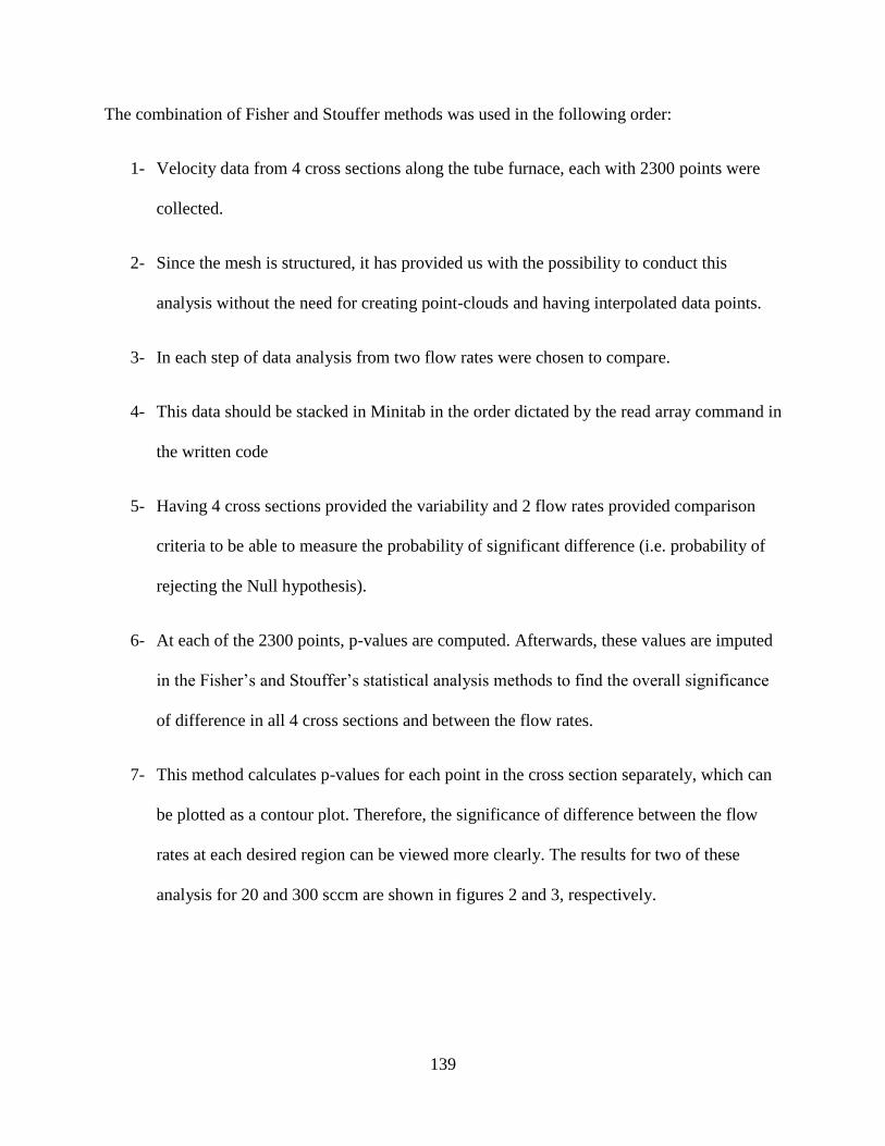
139
The combination of Fisher and Stouffer methods was used in the following order:
1- Velocity data from 4 cross sections along the tube furnace, each with 2300 points were
collected.
2- Since the mesh is structured, it has provided us with the possibility to conduct this
analysis without the need for creating point-clouds and having interpolated data points.
3- In each step of data analysis from two flow rates were chosen to compare.
4- This data should be stacked in Minitab in the order dictated by the read array command in
the written code
5- Having 4 cross sections provided the variability and 2 flow rates provided comparison
criteria to be able to measure the probability of significant difference (i.e. probability of
rejecting the Null hypothesis).
6- At each of the 2300 points, p-values are computed. Afterwards, these values are imputed
in the Fisher’s and Stouffer’s statistical analysis methods to find the overall significance
of difference in all 4 cross sections and between the flow rates.
7- This method calculates p-values for each point in the cross section separately, which can
be plotted as a contour plot. Therefore, the significance of difference between the flow
rates at each desired region can be viewed more clearly. The results for two of these
analysis for 20 and 300 sccm are shown in figures 2 and 3, respectively.

140
Overall Static significance (weighted
p-value)
Spatial Static significance
(weighted p-value)
Absolute Value
Compares significance of absolute
value of the parameter by showing a
single weighted p-value.
From P-value contour
significance of absolute
value can be detected
Relative Value
Compares significance of relative value
of the parameter by showing a single
weighted p-value.
From P-value contour
significance of relative value
can be detected

141
Example 1:
$`Fisher's p-value` [1] 0
$`Stouffer's p-value` [1] 0

142
Example 2:
$`Fisher's p-value`
[1] 0
$`Stouffer's p-value`
[1] 0.9998771

143
Box plots and histograms
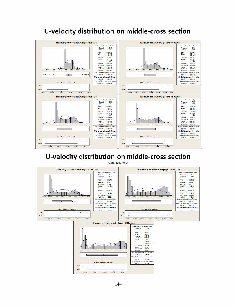
144

145

146

147
Particle injection and residence time distribution function.
Residence time distribution function for 60 sccm inlet gas flow rate is shown in the figure below.
Maximum mean residence time for escaped particles is 400s, however, total mean residence time
is in the order of 1000. Long tail of residence time Distribution function is governed by the
residence time for trapped particles.
Schematics of the studied region for particle tracking and the resulted path-lines for particles are
shown in the next two figures, respectively.
Schematics of Numerical Particle Injection Setup

148
Pathlines of Injected Particles in the Studied Region as a Function of Flow Rate


![Numerical Determination of Two-Phase Material Parameters ... · Numerical Determination of Two-Phase Material Parameters of a ... virtually using methods of stochastic geometry [14],](https://img.dokumen.tips/doc/110x75/5f0f4f6b7e708231d4438708/numerical-determination-of-two-phase-material-parameters-numerical-determination.jpg)