Numerical Heat Transfer, Part A: Applicationslior/lior papers/The Relationship Betwe… · designs. The physics and applications of these devices are detailed in many articles and

This article was downloaded by:[informa internal users]On: 2 April 2008Access Details: [subscription number 755239602]Publisher: Taylor & FrancisInforma Ltd Registered in England and Wales Registered Number: 1072954Registered office: Mortimer House, 37-41 Mortimer Street, London W1T 3JH, UK

Numerical Heat Transfer, Part A:ApplicationsAn International Journal of Computation andMethodologyPublication details, including instructions for authors and subscription information:http://www.informaworld.com/smpp/title~content=t713657973

The Relationship Between the Distributions ofSlot-Jet-Impingement Convective Heat Transfer and theTemperature in the Cooled Solid CylinderNeil Zuckerman a; Noam Lior aa Department of Mechanical Engineering and Applied Science, University ofPennsylvania, Philadelphia, Pennsylvania, USA

Online Publication Date: 01 January 2008To cite this Article: Zuckerman, Neil and Lior, Noam (2008) 'The Relationship Between the Distributions ofSlot-Jet-Impingement Convective Heat Transfer and the Temperature in the Cooled Solid Cylinder', Numerical HeatTransfer, Part A: Applications, 53:12, 1271 - 1293To link to this article: DOI: 10.1080/10407780801960373URL: http://dx.doi.org/10.1080/10407780801960373

PLEASE SCROLL DOWN FOR ARTICLE

Full terms and conditions of use: http://www.informaworld.com/terms-and-conditions-of-access.pdf

This article maybe used for research, teaching and private study purposes. Any substantial or systematic reproduction,re-distribution, re-selling, loan or sub-licensing, systematic supply or distribution in any form to anyone is expresslyforbidden.

The publisher does not give any warranty express or implied or make any representation that the contents will becomplete or accurate or up to date. The accuracy of any instructions, formulae and drug doses should beindependently verified with primary sources. The publisher shall not be liable for any loss, actions, claims, proceedings,demand or costs or damages whatsoever or howsoever caused arising directly or indirectly in connection with orarising out of the use of this material.

http://www.informaworld.com/smpp/title~content=t713657973

http://dx.doi.org/10.1080/10407780801960373

http://www.informaworld.com/terms-and-conditions-of-access.pdf

Dow

nloa

ded

By:

[inf

orm

a in

tern

al u

sers

] At:

13:3

6 2

Apr

il 20

08

THE RELATIONSHIP BETWEEN THE DISTRIBUTIONSOF SLOT-JET-IMPINGEMENT CONVECTIVE HEATTRANSFER AND THE TEMPERATURE IN THECOOLED SOLID CYLINDER

Neil Zuckerman and Noam LiorDepartment of Mechanical Engineering and Applied Science, University ofPennsylvania, Philadelphia, Pennsylvania, USA

A conjugate heat transfer investigation was conducted to better understand the effects of an

impinging radial slot jet cooling device on both the heat transfer rates and temperature

fields in the fluid, and especially in the cylindrical solid cooled by this device. The study used

numerical methods to model a configuration in which a set of four radially positioned slot

jets cooled a cylindrical steel target using air with a jet Reynolds number of 20,000. A

steady-state v2f Reynolds averaged Navier-Stokes model was used with a representative

two-dimensional section of the axisymmetric target and flow domain. Boundary conditions,

heat intensity, target wall thickness, and thermal conductivity were varied to study the

effects of the impingement cooling on the temperature distribution in the solid. For Biot

(Bi) numbers between 0.0025 and 0.073, temperatures in the solid were clearly affected

by lateral conduction, and temperature variation in the solid was an order of magnitude

smaller than the variation in the surface heat transfer coefficient. For the case of constant

heat flux, the area-weighted standard deviation in the solid temperature was found to

correlate well with the dimensionless parameter Z � Bi�d=teq

�2, where d is the cylinder

diameter and teq is the equivalent wall thickness, and a correlation equation was developed.

1. INTRODUCTION

The problem of heating or cooling solid bodies, including those having acurved surface, by impinging jets, is of interest in a variety of manufacturingprocesses and mechanical designs. Impinging jets are used for heat treatment, cool-ing and heating manufactured goods, temperature control of operating machinery,cooling of turbine blades and combustors, drying and defogging, and mass removal.Because of the resulting thinning of the boundary layer and the beneficial effect ofthe generated turbulence, impinging jets may achieve desired heat transfer rates witha flow an order of magnitude lower than conventional parallel-flow heat transferdesigns. The physics and applications of these devices are detailed in many articlesand a number of reviews [1–6]. At least as important as the rates of surface heattransfer and the associated convective heat transfer coefficients for single and

Received 4 April 2007; accepted 4 December 2007.

Address correspondence to Noam Lior, Department of Mechanical Engineering and Applied

Science, University of Pennsylvania, 229 Towne Building, 220 S. 33rd Street, Philadelphia, PA 19104-

6315, USA. E-mail: [email protected]

1271

Numerical Heat Transfer, Part A, 53: 1271–1293, 2008

Copyright # Taylor & Francis Group, LLC

ISSN: 1040-7782 print=1521-0634 online

DOI: 10.1080/10407780801960373

Dow

nloa

ded

By:

[inf

orm

a in

tern

al u

sers

] At:

13:3

6 2

Apr

il 20

08

multiple impinging jets, which have received much attention in the literature, are theresulting temperature and heat transfer distributions in the cooled or heated solid.This temperature distribution may result in phenomena of practical interest, suchas nonuniform material properties, residual thermal stresses, and distortion ofthe target shape [4, 7]. Though numerical models of varying complexity have beendeveloped and exercised to predict the fluid temperature in a variety of jet

NOMENCLATURE

B slot jet nozzle width

Bi Biot number ð¼ht=kÞce2 v2f model constant

CL v2f model constant

Cg v2f model constant

Cm v2f model constant

C1 v2f model constant

C2 v2f model constant

CFD computational fluid

dynamics

d target diameter

D nozzle diameter

D=Dt material derivative

fwall elliptic relaxation function

h convective heat transfer

coefficient

H nozzle-to-target spacing

(nozzle height)

k specific turbulent kinetic

energy

kc fluid thermal conductivity

Lscale turbulence length scale

MAXðrTÞ� nondimensional maximum

temperature gradient

magnitude

n number of jets

nn wall-normal unit vector

Nu Nusselt number

p fluid pressure

ps static pressure

pt total pressure

Pr Prandtl number

Pr0 turbulent Prandtl number

q dynamic pressure (¼qV2=2)

q0 0 heat flux

q0 0 0 heat-generation rate, per unit

volume

r radial position, measured

from jet axis

Re Reynolds number (¼ U0D=nfor a jet)

Sij strain rate tensor

t wall thickness

teq equivalent wall thickness

tscale turbulence time scale

T temperature

TR1, TR2, TR3 temperature ratio functions

U or u fluid velocity component

U0 jet initial speed, average

v fluid velocity

v2 or v2 square of streamwise-normal

velocity fluctuation

x coordinate direction (xi)

y distance from the wall

yþ nondimensional distance

from wall

(¼ ys0:5q0:5n�1)

Z correlation function

[� Bi�

d=teq

�2]

a v2f model constant

e turbulent kinetic energy

dissipation rate

haz azimuth angle

n fluid kinematic viscosity

n0 turbulent kinematic viscosity

q density

r standard deviation function

re v2f model constant

s shear stress

Subscripts

amb ambient

avg average (area-weighted)

i index number for cell or

direction

jet properties at start of

fluid jet

min minimum

max maximum

r radial component (e.g., vr)

t turbulent (e.g., nt)

wall value at target wall outer

surface

h azimuthal component (e.g.,

vh)

0 at stagnation point

1272 N. ZUCKERMAN AND N. LIOR

Dow

nloa

ded

By:

[inf

orm

a in

tern

al u

sers

] At:

13:3

6 2

Apr

il 20

08 impingement problems [8–13], the full conjugate heat transfer problem has been

rarely modeled [14, 15]. As this aspect of impingement heat transfer has receivedlittle attention, its understanding is the main objective of this article.

The specific application of interest here is the cooling of a cylindrical target bysurrounding it with an array of narrow slot jets aligned with the axis of the cylinder(Figure 1). This arrangement offers the potential to improve uniformity of heattransfer on the surface and provide high transfer rates on the entire cylinder surface.Though slot jet impingement has been studied frequently, relatively little has beenpublished about this configuration with this particular nozzle and target combi-nation. Our investigation was numerical. First, we conducted a literature search[5, 6] to understand the strengths and weaknesses of various numerical modelsapplied to impinging jet problems. When using computational fluid dynamics(CFD), the presence, nature, and effects of turbulence are the most uncertain ordifficult-to-model features of impinging jet flows. The available literature containscomparative studies of CFD turbulence models that were conducted with the goalof selecting the model best suited to the impinging-jet heat transfer configuration,though no single model has yet demonstrated all of the desired characteristics[16–19]. Common difficulties include overprediction of Nu in the stagnation regionand underprediction of the intensity and size of the turbulent region in the walljet shear layer, though models with realizability constraints (imposed limits onReynolds stresses) have shown improved results [19].

Following the literature search, we performed CFD simulations of impingingjets. We used several existing time-averaged turbulence models, from the mostcommon to several advanced ones, to examine their performance in simulating jetimpingement cooling of a flat target under a round jet [20, 21], because experimentaldata were available for this configuration and could be used for numerical modelerror assessment (no suitable data were found for a cylindrical target). At theconclusion of this assessment, we selected the v2f model as the best one from the

Figure 1. Isometric view and side view of target and slot jet nozzles.

SIMULATION OF RADIAL JET IMPINGEMENT COOLING 1273

Dow

nloa

ded

By:

[inf

orm

a in

tern

al u

sers

] At:

13:3

6 2

Apr

il 20

08 standpoints of practicality and accuracy for further use (direct numerical simulation

modeling would probably have produced better results but is impractical at this timefor these Reynolds numbers), and constructed numerical models of a cylindricaltarget under various radial slot jet configurations. That study included the fluiddomain only, and calculated the effects on Nusselt number of changes in nozzle size,target curvature, number of nozzles, jet speed, and Prandtl number [20, 21].

The model and other information from [20, 21], describing the convective heattransfer at the surface of a cylindrical target, were then used for the computation ofthe resulting temperature distribution within the solid target. Since there is littleinformation about this temperature distribution, the focus of this article is theconjugate heat transfer study of the relationship between the target’s impingement-induced convective surface heat transfer coefficients (or Nu) field and the targetinterior temperature distributions, as affected by heat conduction in the solid, and,in turn, of the effects of this conduction on the overall heat transfer and temperaturedistribution on the target surface. Specifically, we selected a jet configuration(Re, H=2B, d=D; n) and we varied the geometry and boundary conditions associatedwith the solid target. A significantly narrower scope version of this article waspresented in [25].

2. MODEL CONFIGURATION

2.1. Governing Equations and Numerical Method

The computational model (governing equation set) for the fluid domain wasbased, after careful selection as explained above, on the v2f turbulent fluid modelavailable in Fluent 6.1.22 [22]. This model employs the common eddy-viscositymodel equations for mass conservation and momentum conservation, along withequations for turbulent kinetic energy k, turbulence dissipation rate e, streamwise-normal velocity variance v2, and an elliptic relaxation function f which models theeffects of walls upon v2. The v2f model is unique in that the turbulence-relatedincreases in the diffusion of momentum and thermal energy are tied directly to v2,rather than k (as is done with the k–e model). The development of the importantv2 value is tied to the isotropic turbulent energy k, but also reduced by the presenceof nearby walls via the term f.

As implemented, the model described the time-averaged behavior of an incom-pressible fluid with temperature-independent fluid properties. The governingequations of the v2f model are presented in Eqs. (1)–(13).

qui

qxi¼ 0 ð1Þ

Dui

Dt¼ � qp

qxiþ qqxj

ðnþ n0Þ qui

qxjþ quj

qxi

� �� ð2Þ

DT

Dt¼ q

qxi

nPrþ n0

Pr0

� �qT

qxi

� �ð3Þ


Dow

nloa

ded

By:

[inf

orm

a in

tern

al u

sers

] At:

13:3

6 2

Apr

il 20

08 Dk

Dt¼ q

qxjðnþ n0Þ qk

qxj

� �þ 2n0SijSij � e ð4Þ

DeDt¼ c0e12n0SijSij � ce2e

tscaleþ qqxj

nþ n0

re

� �qeqxj

� �ð5Þ

Dv2

Dt¼ kfwall � v2

ekþ qqxj

ðnþ n0Þ qv2

qxj

" #ð6Þ

fwall � L2scale

qqxj

qf

qxj¼ðC1 � 1Þ

�23� v2

k

�tscale

þ C22n0SijSij

kð7Þ

Sij ¼1

2

qui

qxjþ quj

qxi

� �ð8Þ

Pr0 ¼ 0:5882þ 0:228n0

n

� �� 0:0441

n0

n

� �2�1� e�5:165n=n0�" #�1

ð9Þ

n0 ¼ Cmv2tscale ð10Þ

c0e1 ¼ 1:44 1þ 0:045

ffiffiffiffiffik

v2

s !ð11Þ

Lscale ¼ CL max mink3=2

e;

1ffiffiffi3p k3=2

v2Cmffiffiffiffiffiffiffiffiffiffiffiffiffi2SijSij

p !

;Cgn3

e

� �1=4" #

ð12Þ

tscale ¼ min maxk

e; 6

ffiffiffine

r� �;

affiffiffi3p k

v2Cmffiffiffiffiffiffiffiffiffiffiffiffiffi2SijSij

p" #

ð13Þ

where Cm ¼ 0.19, ce2 ¼ 1.9, re ¼ 1.3, C1 ¼ 1.4, C2 ¼ 0.3, Cg ¼ 70.0, CL ¼ 0.3, anda ¼ 0.6. In our case we solved for steady-state conditions, thus simplifying thematerial derivatives of Eqs. (2–6) to the form uiqðÞ=qxi. Further details of the v2fmodel are given in [23, 24] along with validation comparisons.

The authors had previously compared the v2f model against the experimentaldata set of Baughn and Shimizu [26] to assess the v2f model’s accuracy [21]. It wasfound that the modeling error in the local heat transfer coefficient ranged from2% in the wall jet to 26% in the stagnation region [20]. For the test case used, thetotal error in Nuavg was 8%, averaged by area over the target surface. Additionalstudies were performed to examine the grid sensitivity of the results in the flat-plate


Dow

nloa

ded

By:

[inf

orm

a in

tern

al u

sers

] At:

13:3

6 2

Apr

il 20

08 test case as well as a case with a ring of cylindrical jets, the configuration of interest

described in Section 2.2 [21]. The grid sensitivity of the model was checked by increas-ing cell count and by changing shape functions, allowing either linear or quadraticvariation of flow field properties across quadrilateral cells. Resulting profiles of Nufor the flat-plate model showed that doubling cell density or changing from first-orderto second-order discretization changed local Nu values by no more than 4%, withchanges in Nuavg less than 1%. It was concluded that the model of the cylindricalconfiguration had measurable discretization error and that it affected the secondsignificant figure of Nuavg. Separate studies were performed to examine the influenceof variable fluid properties on Nuavg, by allowing variation in viscosity, density, andthermal conductivity of the fluid (air). For the cases of interest in the range of1 < Twall=Tjet� 4, the resulting Nuavg values changed by up to 3%, a second-ordereffect. These errors were considered acceptable, in view of the uncertainties in theavailable experimental data (such as the turbulence intensity in the approachingjet), and the typical errors in practical heat transfer correlations.

The two-dimensional steady conduction model assumed constant conductivitykc and used the elliptic-type equation

kcqqxi

qT

qxiþ q000 ¼ 0 ð14Þ

for the interior of the solid, where q000 represented a general heat source term indimensions of power per unit volume (e.g., W=m3).

Prior to use of the conjugate heat transfer model within Fluent, the conductionmodel was tested using a cylindrical target similar to the one to be used in theconjugate heat transfer study. The numerical solution was compared to that ofclosed-form analytical solution, and the modeling error of the conduction modelwas found to be less than 1%.

Steady Fluent solutions were performed using the segregated solver withimplicit equations, standard pressure equations, the SIMPLE method forpressure–velocity coupling, and first-order-upwind differencing for the momentum,energy, and turbulent flow characteristics of each quadrilateral cell [22]. Under-relaxation was used for the pressure and momentum equations to provide stableconvergence.

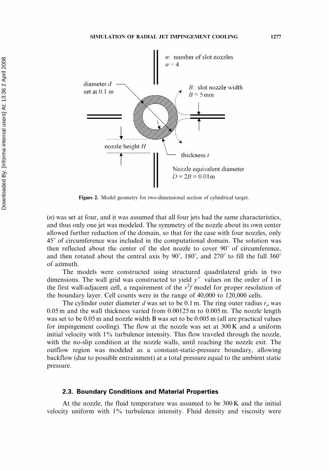
2.2. Geometric Configuration

A numerical model was developed to incorporate a cylindrical body of wallthickness t, which may represent a long annular cylinder of metal being continuouslycooled, as shown in Figure 1. The section of the cylinder was modeled in two dimen-sions, and represented a central section of a cylindrical target located within anenclosure with end walls (Figure 2). The coolant flows within this enclosure. Themean flow velocities were constrained to a planar surface normal to the cylinder axis,and the mean velocity component in the axial direction was set as 0 (no axial flowbecause the cylinder was assumed to be very long). In addition to this assumptionabout symmetry in the axial direction, the geometric symmetry of the cross sectionwas used to reduce the computational domain of the problem. The number of jets


Dow

nloa

ded

By:

[inf

orm

a in

tern

al u

sers

] At:

13:3

6 2

Apr

il 20

08

(n) was set at four, and it was assumed that all four jets had the same characteristics,and thus only one jet was modeled. The symmetry of the nozzle about its own centerallowed further reduction of the domain, so that for the case with four nozzles, only45� of circumference was included in the computational domain. The solution wasthen reflected about the center of the slot nozzle to cover 90� of circumference,and then rotated about the central axis by 90�, 180�, and 270� to fill the full 360�

of azimuth.The models were constructed using structured quadrilateral grids in two

dimensions. The wall grid was constructed to yield yþ values on the order of 1 inthe first wall-adjacent cell, a requirement of the v2f model for proper resolution ofthe boundary layer. Cell counts were in the range of 40,000 to 120,000 cells.

The cylinder outer diameter d was set to be 0.1 m. The ring outer radius ro was0.05 m and the wall thickness varied from 0.00125 m to 0.005 m. The nozzle lengthwas set to be 0.05 m and nozzle width B was set to be 0.005 m (all are practical valuesfor impingement cooling). The flow at the nozzle was set at 300 K and a uniforminitial velocity with 1% turbulence intensity. This flow traveled through the nozzle,with the no-slip condition at the nozzle walls, until reaching the nozzle exit. Theoutflow region was modeled as a constant-static-pressure boundary, allowingbackflow (due to possible entrainment) at a total pressure equal to the ambient staticpressure.

2.3. Boundary Conditions and Material Properties

At the nozzle, the fluid temperature was assumed to be 300 K and the initialvelocity uniform with 1% turbulence intensity. Fluid density and viscosity were

Figure 2. Model geometry for two-dimensional section of cylindrical target.


Dow

nloa

ded

By:

[inf

orm

a in

tern

al u

sers

] At:

13:3

6 2

Apr

il 20

08

set at constant values, which, as discussed in Section 2.1, causes an error of less than3% in the range of parameters examined in this study. This flow through the nozzlewas assigned a no-slip condition at the walls, until reaching the nozzle exit. The out-flow region was modeled as a constant-static-pressure boundary, allowing backflow(due to possible entrainment) at 300 K with a total pressure equal to the ambientstatic pressure. The ambient pressure was set at 1 atm. As the results were correlatedin a nondimensional form, the exact fluid properties were not critical to modelvalidation.

The solid was represented as a material with uniform properties (uniform kc)and no porosity or internal motion (velocity v ¼ 0 within the solid). The energyequation used did not incorporate radiation effects; i.e., it was assumed that thetemperature differences between the solid surface and the fluid were small, and theheat transfer coefficients relatively high, as they indeed were for these cases.

Figure 3. Computational domain for the conjugate heat transfer model.


Dow

nloa

ded

By:

[inf

orm

a in

tern

al u

sers

] At:

13:3

6 2

Apr

il 20

08

Figure 3 shows the computational region with all boundaries and boundary con-ditions.

At the target surface the velocity magnitude was made zero, and, consistentwith conjugate solution methods, continuity of the temperature and heat flux atthe interface between the adjacent solid and fluid cells was imposed.

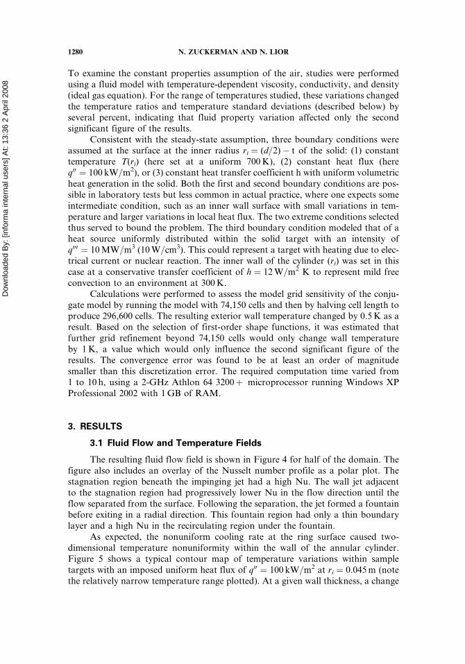
Constant thermal conductivities and densities were selected for the solid andfluid. The conductivity of the steel target was first set at the software default valueof conductivity, kc ¼ 16.27 W=m K. This value corresponded to a 26% nickel steel.To investigate the effect of the thermal conductivity of the solid, runs were also madefor multiple steels with kc from 10 W=m K (such as for a 40% nickel steel) up tokc ¼ 73 W=m K (such as for a high-purity iron). The external flow field was set atRe ¼ 20,000, n ¼ 4, d= D ¼ 10. Parametric variations included type of heatsource, solid material conductivity, material thickness, and heat source intensities.

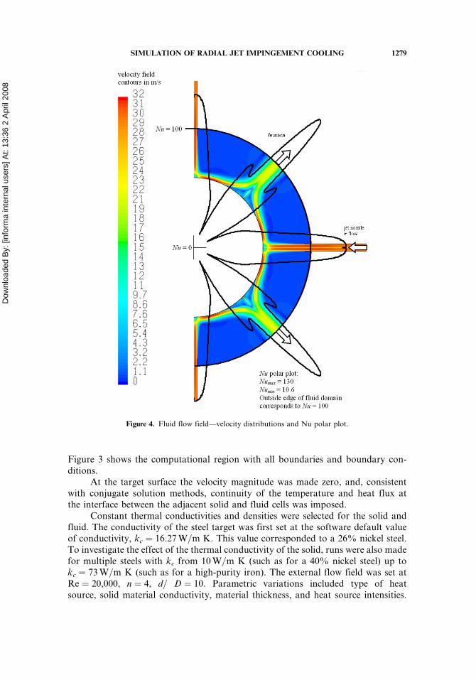
Figure 4. Fluid flow field—velocity distributions and Nu polar plot.


Dow

nloa

ded

By:

[inf

orm

a in

tern

al u

sers

] At:

13:3

6 2

Apr

il 20

08 To examine the constant properties assumption of the air, studies were performed

using a fluid model with temperature-dependent viscosity, conductivity, and density(ideal gas equation). For the range of temperatures studied, these variations changedthe temperature ratios and temperature standard deviations (described below) byseveral percent, indicating that fluid property variation affected only the secondsignificant figure of the results.

Consistent with the steady-state assumption, three boundary conditions wereassumed at the surface at the inner radius ri ¼ (d=2)� t of the solid: (1) constanttemperature T(ri) (here set at a uniform 700 K), (2) constant heat flux (hereq00 ¼ 100 kW=m2), or (3) constant heat transfer coefficient h with uniform volumetricheat generation in the solid. Both the first and second boundary conditions are pos-sible in laboratory tests but less common in actual practice, where one expects someintermediate condition, such as an inner wall surface with small variations in tem-perature and larger variations in local heat flux. The two extreme conditions selectedthus served to bound the problem. The third boundary condition modeled that of aheat source uniformly distributed within the solid target with an intensity ofq000 ¼ 10 MW=m3 (10 W=cm3). This could represent a target with heating due to elec-trical current or nuclear reaction. The inner wall of the cylinder (ri) was set in thiscase at a conservative transfer coefficient of h ¼ 12 W=m2 K to represent mild freeconvection to an environment at 300 K.

Calculations were performed to assess the model grid sensitivity of the conju-gate model by running the model with 74,150 cells and then by halving cell length toproduce 296,600 cells. The resulting exterior wall temperature changed by 0.5 K as aresult. Based on the selection of first-order shape functions, it was estimated thatfurther grid refinement beyond 74,150 cells would only change wall temperatureby 1 K, a value which would only influence the second significant figure of theresults. The convergence error was found to be at least an order of magnitudesmaller than this discretization error. The required computation time varied from1 to 10 h, using a 2-GHz Athlon 64 3200þ microprocessor running Windows XPProfessional 2002 with 1 GB of RAM.

3. RESULTS

3.1 Fluid Flow and Temperature Fields

The resulting fluid flow field is shown in Figure 4 for half of the domain. Thefigure also includes an overlay of the Nusselt number profile as a polar plot. Thestagnation region beneath the impinging jet had a high Nu. The wall jet adjacentto the stagnation region had progressively lower Nu in the flow direction until theflow separated from the surface. Following the separation, the jet formed a fountainbefore exiting in a radial direction. This fountain region had only a thin boundarylayer and a high Nu in the recirculating region under the fountain.

As expected, the nonuniform cooling rate at the ring surface caused two-dimensional temperature nonuniformity within the wall of the annular cylinder.Figure 5 shows a typical contour map of temperature variations within sampletargets with an imposed uniform heat flux of q00 ¼ 100 kW=m2 at ri ¼ 0.045 m (notethe relatively narrow temperature range plotted). At a given wall thickness, a change


Dow

nloa

ded

By:

[inf

orm

a in

tern

al u

sers

] At:

13:3

6 2

Apr

il 20

08

in conductivity changed the range of temperature within the target but otherwise hadsmall influence on the pattern of the temperature contours. A change in thicknesshad a clear influence on the contour map, with a reduction in thickness causingthe contours to be more pronounced in the radial direction, as circumferentialconduction played a smaller role.

We compared our models with those of other impinging jet conjugate heattransfer studies, but due to significant differences in the geometry and physics, wefound only a few similiarities. We briefly compared our steady-state results to thatof the transient conjugate impinging-jet k–x CFD study of Yang and Tsai [14]. Inaddition to the difference between the steady time-averaged and transientapproaches, the two simulations differed in the basic target geometries, jet interac-tion effects, and turbulence models. Our simulations typically had 10 times thenumber of finite-volume cells used in [14]. The Reynolds numbers and solid wall heatfluxes were of the same order of magnitude, and so were the resulting heat transfercoefficients. Both simulations predicted the peak Nu in the stagnation region, but thejet interaction and curved surfaces of our cylindrical target resulted in boundary-layer separation and a fountain flow which brought about important differencesin the Nu profile outside the stagnation region, as displayed in Figure 4. Thelater-time predictions of the transient model in [14] did not show the secondary peakin Nu found in steady-state experimental measurements [26]. During our originalvalidation calculations we found this shortcoming to occur in the majority ofRANS-type turbulence models, and we selected the v2f model because of its abilityto predict the secondary Nu peak, a feature that our models indicate occurs wherethe most turbulent region of the wall jet shear layer contacts the wall surface [21].We also examined the conjugate heat transfer simulations of Rahman et al. [15],which modeled transient heat conduction due to the flow of a liquid free-surface

Figure 5. Typical temperature contours within the solid target in Kelvin for t=d ¼ 0.05,

q00inner ¼ 100 kW=m2, kc ¼ 16.27 W=m K.


Dow

nloa

ded

By:

[inf

orm

a in

tern

al u

sers

] At:

13:3

6 2

Apr

il 20

08 impinging jet at Re ¼ 550 (laminar). This model showed low heat transfer rates in

the center of the stagnation region, a characteristic associated with low turbulenceand low fluid flow speed. In contrast, our high-Re submerged jet case involved amoderately turbulent stagnation region, as do most applications and simulationsof gaseous impinging jets, in which turbulence is used to counteract the poor heattransport properties of stagnant and boundary-layer flows.

3.2. Temperature Variation and Uniformity

There are various ways to express temperature nonuniformity, and theirdefinition and utility depend on the application. The temperature data were thusreduced to four different nondimensional criteria, labeled TR1, TR2, TR3, and r,to describe the temperature nonuniformity in the solid, as shown in Eqs. (15)–(18):

TR1 ¼ Tsolid max

Tsolid minð15Þ

TR2 ¼ Tsolid max � Tsolid min

Tsolid max � Tjetð16Þ

TR3 ¼ Tsolid max � Tsolid min

Tsolid averageð17Þ

r ¼

ffiffiffiffiffiffiffiffiffiffiffiffiffiffiffiffiffiffiffiffiffiffiffiffiffiffiffiffiffiffiffiffiffiffiffiffiffiffiffiffiffiffiPi AiðTi � TaverageÞ2�P

i Ai

�ðT2

averageÞ

vuut ð18Þ

TR1 is the simplest of temperature ratios and incorporates no direct informationabout the external flow field. TR2 shows the ratio of temperature variation withinthe solid to that of the entire problem, yielding a number between 0 and 1. This cre-ates a scale that incorporates the internal source effects and the cooling capability ofthe external flow. TR3 represents the temperature variation in proportion to theaveraged temperature, showing a percent variation in temperature.

In addition to these minimum- or maximum-based functions, the spatial extentof temperature variations within the solid was characterized using a cross-sectional-area-weighted normalized standard deviation, r, defined in Eq. (18), where Ai and Ti

represent the individual cell area and cell-center temperature of each two-dimensional computational model cell. The summation was performed over all cellswithin the solid.

Further, the temperature gradient, which causes internal thermal stresses, wasused as another nonuniformity criterion. Its distribution within the solid, and itsmaximum magnitude (where the highest thermal stresses may occur), were thereforecomputed and mapped for the cases studied. The maximum value of the gradient


Dow

nloa

ded

By:

[inf

orm

a in

tern

al u

sers

] At:

13:3

6 2

Apr

il 20

08 magnitude was nondimensionalized as

MAXðrTÞ� ¼MAX

ffiffiffiffiffiffiffiffiffiffiffiffiffiffiqT

qxj

qT

qxj

s !t

ðTmax � TjetÞð19Þ

and calculated in each cell.A typical temperature gradient magnitude contour map is shown in Figure 6.

The highest T-gradient magnitudes were found in a thin layer of the solid directlyunder the jet and the fountain regions, where h was largest.

When making comparisons, the wall thickness was adjusted to match that of acommon reference, a flat target with equivalent resistance using the equationteq ¼ rinner lnðrouter=rinnerÞ, where r represents a wall radius of the solid. This allowedfor comparison of the radial heat conduction through annular cylinders with slightlydifferent inner wall radii. Various cylinders with equivalent d and equivalent teq

would then have equivalent thermal resistance.

3.3. Influence of Parameters on Temperature Uniformity

The computations were made for the three boundary conditions describedabove. Table 1 lists the selected range of each variable parameter. A total of 37models were used to cover these ranges. Numerical results are shown the Appendix,while the major effects of changing model parameters are summarized in Table 2.Nuavg was found to vary by no more than 3% among the various cases. For allboundary conditions, the maximum and average temperatures within the solidincreased with an increase in source intensity [boundary conditions T(ri), q00, or q000].

Figure 6. Temperature gradient magnitude contour map in K=m for t=d ¼ 0.05, q00inner ¼ 100 kW=m2,

kc ¼ 16.27 W=m K.


Dow

nloa

ded

By:

[inf

orm

a in

tern

al u

sers

] At:

13:3

6 2

Apr

il 20

08

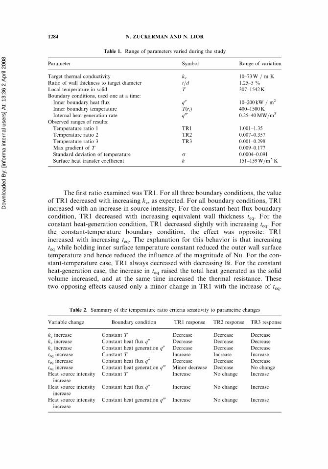
The first ratio examined was TR1. For all three boundary conditions, the valueof TR1 decreased with increasing kc, as expected. For all boundary conditions, TR1increased with an increase in source intensity. For the constant heat flux boundarycondition, TR1 decreased with increasing equivalent wall thickness teq. For theconstant heat-generation condition, TR1 decreased slightly with increasing teq. Forthe constant-temperature boundary condition, the effect was opposite: TR1increased with increasing teq. The explanation for this behavior is that increasingteq while holding inner surface temperature constant reduced the outer wall surfacetemperature and hence reduced the influence of the magnitude of Nu. For the con-stant-temperature case, TR1 always decreased with decreasing Bi. For the constantheat-generation case, the increase in teq raised the total heat generated as the solidvolume increased, and at the same time increased the thermal resistance. Thesetwo opposing effects caused only a minor change in TR1 with the increase of teq.

Table 2. Summary of the temperature ratio criteria sensitivity to parametric changes

Variable change Boundary condition TR1 response TR2 response TR3 response

kc increase Constant T Decrease Decrease Decrease

kc increase Constant heat flux q00 Decrease Decrease Decrease

kc increase Constant heat generation q00 Decrease Decrease Decrease

teq increase Constant T Increase Increase Increase

teq increase Constant heat flux q00 Decrease Decrease Decrease

teq increase Constant heat generation q000 Minor decrease Decrease No change

Heat source intensity

increase

Constant T Increase No change Increase


increase

Constant heat flux q00 Increase No change Increase


increase

Constant heat generation q000 Increase No change Increase

Table 1. Range of parameters varied during the study

Parameter Symbol Range of variation

Target thermal conductivity kc 10–73 W = m K

Ratio of wall thickness to target diameter t=d 1.25–5 %

Local temperature in solid T 307–1542 K

Boundary conditions, used one at a time:

Inner boundary heat flux q00 10–200 kW = m2

Inner boundary temperature T(ri) 400–1500 K

Internal heat generation rate q000 0.25–40 MW=m3

Observed ranges of results:

Temperature ratio 1 TR1 1.001–1.35



Max gradient of T 0.009–0.177

Standard deviation of temperature r 0.0004–0.091

Surface heat transfer coefficient h 151–159 W=m2 K


Dow

nloa

ded

By:

[inf

orm

a in

tern

al u

sers

] At:

13:3

6 2

Apr

il 20

08 For the constant heat flux boundary condition, an increase in teq caused an increase

in the target thermal resistance and therefore elevated solid temperatures at theset flux.

Next the effects on TR2 and TR3 were examined. For all cases, the values ofTR2 and TR3 decreased with increasing kc (as expected and also seen for TR1). Forall three boundary conditions, the value of TR3 increased with an increase in sourceintensity. The value of TR2, however, showed no significant change with sourceintensity for all three boundary conditions. This is understood from the fact thatTR2 incorporated information about the full temperature scale of the problem fromTmax to Tjet and thus became insensitive to the changes in Tmax resulting from heatsource intensity increases; TR2 was intended to scale with source intensity. For thecase with constant heat flux, the values of both TR2 and TR3 decreased with increas-ing teq. This resulted primarily from the increase in the Tmax or Tavg value caused byforcing the same flux through a higher resistance. For the case of constant heatgeneration, the value of TR2 decreased with increasing teq, but TR3 did not varywith teq. The effect on TR2 in this case resulted from scaling the model results withTmax, while the increase in thickness lowered the relative value of Tmin. The minimaleffect on TR3 was attributed to the competing influences of higher resistance andhigher total power generation. For the constant-temperature boundary condition,the values of TR2 and TR3 both increased with increasing teq. This case was onceagain the opposite of the constant heat flux boundary condition, so increasing t ata given Tmax produced a higher temperature drop through the target, allowing alower Tmin on the surface due to the increased relative influence of external convec-tion (higher Bi). In comparison with TR2 and TR3, the majority of the values forTR1 had a small dynamic range. From this we concluded that TR3 provided a moreuseful and meaningful measure of the variation in surface temperature.

For all cases, an increase in kc decreased the maximum gradient intensity, asexpected. The method of nondimensionalizing the gradient magnitude made itinvariant to source intensity. For all three boundary conditions, the magnitude ofthe maximal gradient increased with increasing teq. For the majority of cases, teq

was within a few percent of t. Comparisons between models were performed usingthe Biot number defined as Bi ¼ hteq=kc solid. Given the high conductivity of themetal target, the Bi for this application ranged from 0.0025 to 0.073. As a result,lateral conduction played an important role in smoothing out temperature variationsin the solid. This effect is illustrated by the example profiles of T and Nu on theouter surface for the constant heat flux boundary condition, shown in Figure 7for an example case with wall thickness t=d ¼ 0.05. A comparable effect is seen inFigure 8 which shows inner and outer wall temperatures for the constant-temperature boundary condition at wall thicknesses t=d ¼ 0.05 and t=d ¼ 0.025.As the value of t increased and the outer surface temperature minima decreased,the regions of peak outer surface temperature also shifted farther away from thestagnation region.

Even though the local Nu varied by a factor of 10, the temperature variationsin the solid were in the range of one-quarter to one-tenth of the overall temperaturerange in the problem. The regions of high fluid temperature (within 10% of the walltemperature) occupied only a small portion of the fluid volume within the computa-tional domain boundary, shown in Figure 9, as the heat rapidly dropped off within


Dow

nloa

ded

By:

[inf

orm

a in

tern

al u

sers

] At:

13:3

6 2

Apr

il 20

08

the thermal boundary layer. The resulting Nu profile for the conjugate problem wasvery close to that found in the case of zero wall thickness [20, 21], with variations inNu between cases in the studied range of only 1–3%. This showed that, within therange of variable values considered, conduction in the solid in the analysis has anegligible effect on the flow and heat transfer in the fluid, and on the convective heat

Figure 8. Nusselt number and temperature profiles on outer surface for t=d ¼ 0.05 and 0.025, T(ri) ¼700 K, kc ¼ 16.27 W=m K.

Figure 7. Nusselt number and temperature profiles on outer surface for t=d ¼ 0.05, q00inner ¼ 100 kW=m2,

kc ¼ 16.27 W=m K.


Dow

nloa

ded

By:

[inf

orm

a in

tern

al u

sers

] At:

13:3

6 2

Apr

il 20

08

transfer coefficient on the solid interface. One practical conclusion is that it is notnecessary to consider the conjugate problem if only the fluid dynamics and heattransfer in the fluid are of interest.

The Biot number Bi serves a useful purpose in describing the expected tempera-tures in the target. Further examination of the influence of kc and t on the heat

Figure 9. Contour map of temperature T in Kelvin for t=d ¼ 0.05, q00inner ¼ 100 kW=m2, kc ¼ 16.27 W=m

K.

Figure 10. Standard deviation of temperature r versus Z for t=d ¼ 0.050, 0.025, and 0.0125, kc from

10 to 73 W=m K.


Dow

nloa

ded

By:

[inf

orm

a in

tern

al u

sers

] At:

13:3

6 2

Apr

il 20

08 distribution led to the conclusion that parameters describing uniformity of tempera-

ture did not and should not correlate with Bi, if we define Bi as Bi ¼ hteq=kc. Ingeneral, the Biot number described the relative importance or strength of externalconvective transfer rate (h) to internal conductive heat transfer (kc=teq). It did notincorporate any direct information regarding the uniformity within the target. Toexplain, as kc is increased, and hence Bi decreased, it would be expected to obtaina more uniform temperature field within the solid target. Yet if t was increased,and Bi thus increased, it would also be expected to see a more uniform temperaturewithin the target. So, a highly uniform temperature field could be associated witheither high or low Bi, meaning Bi alone does not provide information allowingone to draw a conclusion about the expected temperature uniformity.

As stated above, the uniformity of the temperature was expected to increaseboth with increasing kc and with increasing teq. Based on this relationship, a newnondimensional parameter was selected:

Z ¼ hðd2Þkteq

¼ Bid

teq

� �2

ð20Þ

Because of the varying lateral conduction effects for the cylindrical geometry atdifferent nondimensional thicknesses (t=d), the value of thickness t used in Eq. (20)was the equivalent flat-plate thickness teq.

Comparison of r values versus Z for different kc and t using the constant heatflux boundary condition showed a successful correlation, with all points falling on asingle curve. One should note that the influence of variations in h and the nonunifor-mity of the h profile on r were not investigated in this study. For this reason, theinclusion of h in the numerator was for convenience only; further studies shouldmore thoroughly define the functional dependence on h (and thus k, t, n, Re, andt=d) and redefine the form of Z. Future work could then produce a new form ofthe Z function which would incorporate all of these independent variables, replacingh with another function, perhaps in a form incorporating both hmax and hmin. The rdata for the other two boundary conditions did not correlate well with the form of Zshown in Eq. (20). It is likely that with more parameters incorporated into the Zfunction, it can be reformulated for problems with all three boundary conditions.Figure 10 shows the trend of r versus Z for the constant heat flux boundarycondition.

4 CONCLUSIONS

A conjugate heat transfer study of the effects of multiple (4) axial slot coolingjet impingement on a hot long cylindrical pipe was conducted. The study examinedthe temperature distributions and nonuniformities in the solid cylinder wallfor Re ¼ 20,000, 10 W=m K� kc� 73 W=m K, 0.0125� t=d� 0.0500, 0.0025�Bi� 0.073, and 4.4�Z� 129. Despite the relatively large temperature difference ofup to 400 K between the cooling fluid and the solid surface, the conduction in thesolid was found to have a negligible effect on the flow and heat transfer in the fluid,and on the convective heat transfer coefficient on the solid interface. One practical


Dow

nloa

ded

By:

[inf

orm

a in

tern

al u

sers

] At:

13:3

6 2

Apr

il 20

08 conclusion is that, for the range of parameters used in this study, it is not necessary

to consider the conjugate problem if only the fluid dynamics and heat transfer in thefluid are of interest.

For the constant heat flux boundary condition on the internal pipe surface, thedimensionless parameter Z � Biðd=teqÞ2 was found to correlate well the internal tem-perature nonuniformity standard deviation r with the values of kc and t=d in thatrange. Defining and using several nonuniformity evaluation criteria, we found initialindications of the importance of lateral conduction in an annular cylinder cooled byradial impinging jets. For the cases studied herein, the lateral conduction played animportant role in making the temperature nonuniformity in the solid an order ofmagnitude smaller than the nonuniformity in the surface Nu caused by theimpinging jets.

REFERENCES

1. H. Martin, Heat and Mass Transfer between Impinging Gas Jets and Solid Surfaces, Adv.Heat Transfer, vol. 13, pp. 1–60, 1977.

2. K. Jambunathan, E. Lai, M. A. Moss, and B. L. Button, A Review of Heat Transfer Datafor Single Circular Jet Impingement, Int. J. Heat Fluid Flow, vol. 13, pp. 106–115, 1992.

3. R. Viskanta, Heat Transfer to Impinging Isothermal Gas and Flame Jets, Exp. ThermalFluid Sci., vol. 6, pp. 111–134, 1993.

4. J. Ferrari, N. Lior, and J. Slycke, An Evaluation of Gas Quenching of Steel Rings byMultiple-Jet Impingement, J. Mater. Process. Technol., vol. 136, pp. 190–201, 2003.

5. N. Zuckerman and N. Lior, Impingement Heat Transfer: Correlations and NumericalModeling, ASME J. Heat Transfer, vol. 127, pp. 544–552, 2005.

6. N. Zuckerman and N. Lior, Jet Impingement Heat Transfer: Physics, Correlations, andNumerical Modeling, Adv. Heat Transfer, vol. 39, pp. 565–632, 2006.

7. H. Laschefski, T. Cziesla, G. Biswas, and N. K. Mitra, Numerical Investigation of HeatTransfer by Rows of Rectangular Impinging Jets, Numer. Heat Transfer A, vol. 30,pp. 87–101, 1996.

8. T. Cziesla, E. Tandogan, and N. K. Mitra, Large-Eddy Simulation of Heat Transfer fromImpinging Slot Jets, Numer. Heat Transfer A, vol. 32, pp. 1–17, 1997.

9. A. Y. Tong, A Numerical Study on the Hydrodynamics and Heat Transfer of a CircularLiquid Jet Impinging onto a Substrate, Numer. Heat Transfer A, vol. 44, pp. 1–19, 2003.

10. N. Lior, The Cooling Process in Gas Quenching, J. Mater. Process. Technol., vol. 155–156,pp. 1881–1888, 2004.

11. D. Sahoo and M. A. R. Sharif, Mixed-Convective Cooling of an Isothermal Hot Surfaceby Confined Slot Jet Impingement, Numer. Heat Transfer A, vol. 45, pp. 887–909, 2004.

12. I. Sezai and L. B. Y. Aldabbagh, Three-Dimensional Numerical Investigation of Flow andHeat Transfer Characteristics of Inline Jet Arrays, Numer. Heat Transfer A, vol. 45,pp. 271–288, 2004.

13. S. A. Salamah and D. A. Kaminski, Modeling of Turbulent Heat Transfer from an Arrayof Submerged Jets Impinging on a Solid Surface, Numer. Heat Transfer A, vol. 48,pp. 315–337, 2005.

14. Y.-T. Yang and S.-Y. Tsai, Numerical Study of Transient Conjugate Heat Transfer of aTurbulent Impinging Jet, Int. J. Heat Mass Transfer, vol. 50, pp. 799–807, 2007.

15. M. M. Rahman and A. J. Bula, Analysis of Transient Conjugate Heat Transfer to a FreeImpinging Jet, AIAA J. Thermophys. Heat Transfer, vol. 14, pp. 330–339, 2000.


Dow

nloa

ded

By:

[inf

orm

a in

tern

al u

sers

] At:

13:3

6 2

Apr

il 20

08 16. S. Polat, B. Huang, A. S. Mujumdar, and W. J. M. Douglas, Numerical Flow and Heat

Transfer under Impinging Jets: A Review, Annu. Rev. Fluid Mech. Heat Transfer, vol. 2,pp. 157–197, 1989.

17. T. J. Craft, L. J. W. Graham, and B. E. Launder, Impinging Jet Studies for TurbulenceModel Assessment—Part 2, An Examination of the Performance of Four TurbulenceModels, Int. J. Heat Mass Transfer, vol. 36, pp. 2685–2697, 1993.

18. S. Z. Shuja, B. S. Yilbas, and M. O. Budair, Gas Jet Impingement on a Surface Having aLimited Constant Heat Flux Area: Various Turbulence Models, Numer. Heat Transfer A,vol. 36, pp. 171–200, 1999.

19. A. Abdon and B. Sunden, Numerical Investigation of Impingement Heat Transfer UsingLinear and Nonlinear Two-Equation Turbulence Models, Numer. Heat Transfer A,vol. 40, pp 563–578, 2001.

20. N. Zuckerman and N. Lior, Jet Impingement Heat Transfer on a Circular Cylinder byRadial Slot Jets, Proc. IMECE05, 2005 ASME Int. Mechanical Engineering Congressand Exposition, Orlando, FL, November 5–11, 2005.

21. N. Zuckerman and N. Lior, Radial Slot Jet Impingement Flow and Heat Transfer on aCylindrical Target, AIAA J. Thermophysics Heat Transfer, vol. 21, pp. 548–561, 2007.

22. Fluent, Inc., Fluent 6.1 User’s Guide, 01-25-2003, 2003.23. P. A. Durbin, A Reynolds Stress Model for Near-Wall Turbulence, J. Fluid Mech.,

vol. 249, pp. 465–498, 1993.24. P. Durbin, Separated Flow Computations with the k-E-v2 Model, AIAA J., vol. 33,

pp. 659–664, 1995.25. N. Zuckerman and N. Lior, Heat Transfer and Temperature Distributions in the Fluid

and Cooled Cylindrical Solid during Radial Slot Jet Impingement Cooling, PaperJET-05, 13th Int. Heat Transfer Conf., Sydney, Australia, August 13–18, 2006.

26. J. W. Baughn and S. Shimizu, Heat Transfer Measurements from a Surface with UniformHeat Flux and an Impinging Jet, ASME J. Heat Transfer, vol. 111, pp. 1096–1098, 1989.


Dow

nloa

ded

By:

[inf

orm

a in

tern

al u

sers

] At:

13:3

6 2

Apr

il 20

08

AP

PE

ND

IX

Ta

ble

s3

,4

,a

nd

5p

rese

nt

qu

an

tita

tiv

ere

sult

so

fth

esi

mu

lati

on

sw

ith

va

rio

us

pa

ram

etri

cch

an

ges

.

Tab

le3

.R

esu

lts

fro

mth

eco

nju

gat

eh

eat

tra

nsf

erp

rob

lem

,co

nst

ant

hea

tfl

ux

bo

un

da

ryco

nd

itio

n

Co

nst

an

t

tem

per

atu

ren¼

4;d¼

0:1

m;R

e jet¼

20;0

00;

Tje

t¼

30

0K

TR

1T

R2

TR

3

Bo

un

da

ry

con

dit

ion

kc

W=

mK

t eq=d

t=d

NU

avg

ZB

i avg

Tm

ax=

Tm

in

So

lid

tem

per

atu

re

ran

ge

(Tm

ax�

Tm

in)=

(Tm

ax�

Tje

t)

So

lid

tem

per

atu

re

ran

ge

(Tm

ax�

Tm

in)=

(Tavg

soli

d)

Ma

xte

mp

.

gra

die

nt

(no

n-d

imen

sio

nal)

rnr

ma

x

nr

min

Tm

ax

in

soli

d

K

Tavg

inso

lid

K

q00¼

10

0k

W=m

27

30

.04

74

0.0

50

06

34

.40

.00

981

.02

0.0

33

0.0

22

0.0

29

0.0

05

12

.3�

2.1

90

98

98

q00¼

10

0k

W=m

25

90

.04

74

0.0

50

06

35

.40

.01

221

.03

0.0

41

0.0

28

0.0

35

0.0

06

32

.3�

2.1

91

28

98

q00¼

10

0k

W=m

23

50

.04

74

0.0

50

06

39

.20

.02

061

.05

0.0

66

0.0

46

0.0

58

0.0

10

52

.3�

2.1

92

18

99

q00¼

10

0k

W=m

21

90

.04

74

0.0

50

06

31

7.0

0.0

382

1.0

90

.11

50

.08

20

.10

00

.01

85

2.4�

2.1

94

19

01

q00¼

10

0k

W=m

21

60

.04

74

0.0

50

06

31

9.9

0.0

447

1.1

00

.13

20

.09

50

.11

40

.02

13

2.4�

2.1

94

89

02

q00¼

10

0k

W=m

21

00

.04

74

0.0

50

06

43

2.6

0.0

733

1.1

60

.19

70

.14

80

.17

00

.03

27

2.4�

2.1

97

79

05

q00¼

10

0k

W=m

27

30

.02

44

0.0

25

06

38

.60

.00

511

.03

0.0

47

0.0

33

0.0

13

0.0

09

71

.8�

1.6

94

49

27

q00¼

10

0k

W=m

23

50

.02

44

0.0

25

06

31

8.0

0.0

107

1.0

70

.09

30

.06

60

.02

60

.01

94

1.8�

1.6

95

99

27

q00¼

10

0k

W=m

21

90

.02

44

0.0

25

06

43

3.5

0.0

199

1.1

20

.15

70

.11

50

.04

60

.03

33

1.9�

1.6

98

39

25

q00¼

10

0k

W=m

21

60

.02

44

0.0

25

06

43

9.2

0.0

233

1.1

40

.17

70

.13

20

.05

30

.03

79

1.9�

1.6

99

19

25

q00¼

10

0k

W=m

21

00

.02

44

0.0

25

06

56

4.6

0.0

384

1.2

20

.25

30

.19

80

.08

00

.05

57

1.9�

1.6

10

23

92

4

q00¼

10

0k

W=m

27

30

.01

23

0.0

12

56

31

6.9

0.0

026

1.0

60

.08

50

.06

10

.00

90

.01

89

1.6�

1.6

97

69

48

q00¼

10

0k

W=m

23

50

.01

23

0.0

12

56

43

5.6

0.0

054

1.1

20

.15

70

.11

70

.01

80

.03

62

1.6�

1.6

10

01

94

6

q00¼

10

0k

W=m

21

60

.01

23

0.0

12

56

57

8.2

0.0

119

1.2

40

.27

10

.21

40

.03

40

.06

60

1.7�

1.6

10

45

94

2

q00¼

10

0k

W=m

21

00

.01

23

0.0

12

56

61

29

.20

.01

971

.35

0.3

57

0.2

98

0.0

50

0.0

91

01

.7�

1.6

10

86

94

0

q00¼

10

kW=m

23

50

.04

74

0.0

50

06

39

.20

.02

061

.01

0.0

65

0.0

11

0.0

58

0.0

02

62

.2�

2.0

36

23

60

q00¼

20

0k

W=m

23

50

.04

74

0.0

50

06

39

.20

.02

061

.06

0.0

66

0.0

55

0.0

58

0.0

12

52

.3�

2.1

15

42

14

99

1291

Dow

nloa

ded

By:

[inf

orm

a in

tern

al u

sers

] At:

13:3

6 2

Apr

il 20

08

Tab

le4

.R

esu

lts

fro

mth

eco

nju

ga

teh

eat

tra

nsf

erp

rob

lem

,co

nst

ant

hea

t-g

ener

ati

on

con

dit

ion

Co

nst

an

t

tem

per

atu

ren¼

4;d¼

0:1

m;R

e jet¼

20;0

00;

Tje

t¼

30

0K

TR

1T

R2

TR

3

Bo

un

da

ry

con

dit

ion

kc

W=m

Kt e

q=d

t=d

NU

avg

ZB

i avg

Tm

ax=

Tm

in

So

lid

tem

per

atu

re

ran

ge

(Tm

ax�

Tm

in)=

(Tm

ax�

Tje

t)

So

lid

tem

per

atu

re

ran

ge

(Tm

ax�

Tm

in)=

(Tavg

soli

d)

Ma

xte

mp

.

gra

die

nt

(no

n-d

imen

sio

nal)

rnr

ma

x

nr

min

Tm

ax

in

soli

d

K

Tavg

inso

lid

K

q000¼

10

MW=m

37

30

.04

740

.05

006

34

.40

.00

981

.01

0.0

27

0.0

14

0.0

29

0.0

036

1.8�

2.0

59

85

94

q000¼

10

MW=m

35

90

.04

740

.05

006

35

.40

.01

221

.02

0.0

34

0.0

17

0.0

36

0.0

044

1.8�

2.0

59

95

94

q000¼

10

MW=m

33

50

.04

740

.05

006

39

.20

.02

061

.03

0.0

55

0.0

28

0.0

58

0.0

073

1.8�

2.0

60

25

94

q000¼

10

MW=m

31

90

.04

740

.05

006

31

7.0

0.0

382

1.0

50

.09

60

.05

00

.10

20

.01

281

.8�

2.0

60

85

94

q000¼

10

MW=m

31

00

.04

740

.05

006

43

2.6

0.0

733

1.0

90

.16

40

.08

80

.17

70

.02

251

.9�

2.0

62

05

95

q000¼

10

MW=m

37

30

.02

440

.02

506

38

.60

.00

511

.02

0.0

45

0.0

15

0.0

13

0.0

048

1.6�

1.6

45

34

50

q000¼

10

MW=m

31

00

.02

440

.02

506

56

4.6

0.0

383

1.0

90

.23

60

.08

90

.08

00

.02

711

.7�

1.6

46

94

48

q000¼

0:2

5M

W=m

33

50

.04

740

.05

006

39

.20

.02

061

.00

0.0

54

0.0

01

0.0

58

0.0

004

1.8�

2.0

30

83

07

q000¼

40

MW=m

33

50

.04

740

.05

006

39

.20

.02

061

.05

0.0

55

0.0

45

0.0

58

0.0

117

1.8�

2.0

15

08

14

77

1292

Dow

nloa

ded

By:

[inf

orm

a in

tern

al u

sers

] At:

13:3

6 2

Apr

il 20

08

Ta

ble

5.

Res

ult

sfr

om

the

con

jug

ate

hea

ttr

an

sfer

pro

ble

m,

con

sta

nt-

tem

per

atu

reb

ou

nd

ary

con

dit

ion

Co

nst

an

t

tem

per

atu

ren¼

4;d¼

0:1

m;R

e jet¼

20;0

00;T

jet¼

30

0K

TR

1T

R2

TR

3

Bo

un

da

ry

con

dit

ion

kc

W=m

Kt e

q=d

t=d

NU

avg

ZB

i avg

Tm

ax=

Tm

in

So

lid

tem

per

atu

re

ran

ge

(Tm

ax�

Tm

in)=

(Tm

ax�

Tje

t)

So

lid

tem

per

atu

re

ran

ge

(Tm

ax�

Tm

in)=

(Tavg

soli

d)

Ma

xte

mp

.

gra

die

nt

(no

n-d

imen

sio

na

l)r

nr

ma

x

nr

min

Tm

ax

in

soli

d

K

Tavg

inso

lid

K

Tin

ner

wall¼

70

0K

73

0.0

474

0.0

50

06

24

.40

.00

98

1.0

00

.00

70

.00

40

.02

70

.00

224

.72

.87

00

69

3

Tin

ner

wall¼

70

0K

59

0.0

474

0.0

50

06

25

.40

.01

21

1.0

00

.00

70

.00

40

.03

40

.00

272

.00

.47

00

69

6

Tin

ner

wall¼

70

0K

35

0.0

474

0.0

50

06

39

.10

.02

05

1.0

20

.03

70

.02

10

.05

60

.00

452

.0�

2.7

70

06

94

Tin

ner

wall¼

70

0K

19

0.0

474

0.0

50

06

31

6.9

0.0

37

91

.04

0.0

66

0.0

38

0.0

99

0.0

082

2.0�

2.7

70

06

89

Tin

ner

wall¼

70

0K

16

0.0

474

0.0

50

06

31

9.7

0.0

44

31

.05

0.0

77

0.0

45

0.1

14

0.0

095

2.0�

2.7

70

06

87

Tin

ner

wall¼

70

0K

10

0.0

474

0.0

50

06

33

2.2

0.0

72

41

.07

0.1

19

0.0

70

0.1

76

0.0

150

2.0�

2.7

70

06

79

Tin

ner

wall¼

70

0K

73

0.0

244

0.0

25

06

38

.50

.00

51

1.0

10

.01

00

.00

60

.01

10

.00

122

.0�

3.0

70

06

98

Tin

ner

wall¼

70

0K

16

0.0

244

0.0

25

06

33

8.3

0.0

22

81

.03

0.0

44

0.0

25

0.0

47

0.0

052

1.9�

3.0

70

06

93

Tin

ner

wall¼

70

0K

10

0.0

244

0.0

25

06

36

2.6

0.0

37

11

.04

0.0

69

0.0

40

0.0

75

0.0

082

1.9�

3.0

70

06

89

Tin

ner

wall¼

40

0K

35

0.0

474

0.0

50

06

39

.10

.02

05

1.0

10

.03

70

.00

90

.05

60

.00

202

.0�

2.7

40

03

98

Tin

ner

wall¼

15

00

K3

50

.04

740

.05

00

63

9.1

0.0

20

51

.03

0.0

37

0.0

30

0.0

56

0.0

064

2.0�

2.7

15

00

14

81

1293

Documents

Numerical Heat Transfer, Part A: Applicationslior/lior papers/The Relationship Betwe… · designs. The physics and applications of these devices are detailed in many articles and