Numerical-analytical solutions of predator-prey … solutions of predator-prey models GILBERTO GONZALEZ-PARRA´ Grupo de Matem´atica Multidisciplinar (GMM) Dpto. Calculo, Facultad

Numerical-analytical solutions of predator-prey models

GILBERTO GONZALEZ-PARRAGrupo de Matematica Multidisciplinar (GMM)

Dpto. Calculo, Facultad IngenierıaUniversidad de los Andes

Hechicera, [email protected]

ABRAHAM J. ARENASDepartamento de Matematicas y Estadıstica

Universidad de CordobaGrupo Tesseo, Universidad del Sinu

Monterıa, CordobaCOLOMBIA

[email protected]

MYLADIS R. COGOLLODepartamento de Ciencia Basica

Universidad EAFITMedellın

[email protected]

Abstract:- This paper deals with the construction of piecewise analytic approximate solutions for nonlinear initialvalue problems modeled by a system of nonlinear ordinary differential equations. In real world several biologicaland environmental parameters in the predator-prey model vary in time. Thus, non-autonomous systems are impor-tant to be studied. We show the effectiveness of the method for autonomous and non-autonomous predator-preysystems. The method we have used is called the differential transformation method which has some suitable prop-erties such as accuracy, low computational cost, easiness of implementation and simulation as well as preservingproperties of the exact theoretical solution of the problem. The accuracy of the method is checked by numericalcomparison with fourth-order Runge-Kutta results applied to several predator-prey examples.

Key–Words: Differential transformation method, Population dynamics, Nonlinear differential system, Predator-prey system.

1 Introduction

The modeling biological systems is commonly basedon systems of nonlinear ordinary differential equa-tions. Mathematical models and their simulation areimportant to understand qualitatively and quantita-tively these systems. The study of biological phe-nomena such as harvesting of populations and avail-ability of biological resources is relevant for the eco-logical life and for several human activities such asforestry, fishery and others. Therefore, it is impor-tant to investigate models that include interactions be-tween species. The predator-prey models are one ofthe most well known and were constructed indepen-dently by Lotka(1925) and Volterra(1926) [1]. There

are many different kind of predator-prey models inthe mathematical ecology literature including continu-ous and discrete models, and several works have beendevoted to investigate these models regarding peri-odicity, global stability boundedness and others fea-tures [2]. It is important to remark that realistic mod-els often require the effects of the changing environ-ment giving rise to non-autonomous nonlinear ordi-nary differential equation systems. The aim of thispaper is to investigate numerically the reliability andconvenience of the differential transformation method(DTM ) applied to predator-prey models governed bythe following two-dimensional system of nonlinear

WSEAS TRANSACTIONS on BIOLOGY and BIOMEDICINE Gilberto Gonzalez-Parra, Abraham J. Arenas, Myladis R. Cogollo

E-ISSN: 2224-2902 79 Issue 2, Volume 10, July 2013

ordinary differential equations{x1(t) = f(x1(t), x2(t), a1(t), · · ·, an(t)),x2(t) = g(x1(t), x2(t), b1(t), · · ·, bn(t)),

(1)

where x1(t), x2(t) represent the population densitiesat time t of prey and predator respectively and thepositive functions ai(t), bi(t) generally give relativemeasures of the effect of dimensional parameters [1].Due to the structure of the functions f and g, the so-lution of system (1) is not trivial, therefore it is nec-essary to develop reliable numerical techniques to ob-tain their numerical solutions. The numerical solu-tion of predator-prey models has been treated in sev-eral papers in order to investigate numerically the re-liability and efficiency of different methods. For in-stance in [3, 4, 5, 6] the Adomian method has beentested numerically using a predator-prey model. Ad-ditionally, in [7] He’s variational method was studiedand applied to a predator-prey model. The nonstan-dard finite difference schemes has been applied alsoto the predator-prey model [8]. In [9] the DTM wasapplied to a predator-prey model with constant coeffi-cients over a short time horizon. However in this pa-per, in order to illustrate the accuracy of the method,DTM is applied to autonomous and non-autonomouspredator-prey models over long time horizons and theobtained results are compared with the fourth-orderRunge-Kutta method, and when are available with theanalytical exact solutions. It is shown that the DTMis easy to apply and its numerical solutions preservethe properties of the continuous models, such as pe-riodic behaviors. In addition this method is applieddirectly to the nonlinear ordinary differential equa-tion system without requiring linearization, discretiza-tion or perturbation. The DTM was first proposedby Zhou [10], and its main application therein is tosolve initial value problems in electrical circuits andhas been applied to solve a variety of problems thatarise from differential equations [11, 12, 13, 14]. TheMichaelis-Menten equation that describes the rate ofdepletion of the substrate of interest has been solvedusing the DTM in [15] and authors show that theDTM is accurate and easy to apply for this particulardifferential equation.

The DTM develops from the differential equa-tion system with initial conditions a recurrence equa-tion system that finally leads to the solution of a sys-tem of algebraic equations as coefficients of a powerseries solution. It is important to remark that theDTM does not evaluate the derivatives symbolically;instead, it calculates the relative derivatives by an it-eration procedure described by the transformed equa-tions obtained from the original equations using dif-ferential transformation. In order to improve the rate

of convergence and improve the accuracy of the cal-culations, it is convenient to divide the entire domainH into n sub-domains. The main advantage of do-main split process is that only a few series terms arerequired to compose the solution in a small time in-terval Hi. Thus, the system of differential equationscan then be solved in each sub-domain. Thus, afterthe recurrence equation system has been solved, eachsolution xj(t) can be obtained by a finite-term Taylorseries. Unlike the conventional high order Taylor se-ries method which requires a lot of symbolic compu-tations, the DTM is performed iteratively [14]. How-ever, the method have some drawbacks, which can beovercome by splitting the domain region into subinter-vals in order to obtain accurate solutions [12, 14]. Inaddition, some complex nonlinear models are difficultto be solved by the DTM . In [16] it has been pro-posed a new formula for these complex models. TheDTM has been applied recently to integral equationsystems [17]. Furthermore, the DTM was introducedrecently in the area of random differential equations[18]. In particular has been used to solve the Riccatirandom differential equation in [19].

The number of sub-domains n has to be chosen inan appropriate form in order to obtain accurate solu-tions. Similar methods choose the value of n and thenumber of terms to obtain a given admissible globalerror given a priori. Other related works have pro-posed a strategy with few terms in each subintervaland a high number of sub-domains n [20]. Here,we follow a similar strategy only to show the ef-fectiveness of the DTM for autonomous and non-autonomous predator-prey systems.

Since, several biological and environmental pa-rameters in the predator-prey model vary in time, non-autonomous systems are important to be studied. Inthis paper three predator-prey models are consideredin order to study numerically the reliability of theDTM applied to these type of models.

The organization of this paper is as follows. InSection 2, basic definitions of the DTM and some ba-sic properties of the DTM are presented. Section 3 isdevoted to present the numerical results of the applica-tion of the method to different predator-prey systems.Comparisons between the DTM and the fourth-orderRunge-Kutta (RK4) solutions are shown. Finally inSection 4 discussion and conclusions are presented.



2 Basic definitions and propertiesof differential transformationmethod

For clarity of presentation of the DTM , we summa-rize the main issues of the method that may be foundin [10].

Definition 1 Let x(t) be analytic in the time domainD, then it has derivatives of all orders with respect totime t. Put

φ(t, k) =dkx(t)

dtk, ∀t ∈ D. (2)

For t = ti, then φ(t, k) = φ(ti, k), where k be-longs to a set of non-negative integers, denoted as theK domain. Thus, (2) can be rewritten as

X(k) = φ(ti, k) =

[dkx(t)

dtk

]t=ti

(3)

where X(k) is called the spectrum of x(t) at t = ti.

Definition 2 Suppose that x(t) is analytic in the timedomain D, then it can be represented as

x(t) =

∞∑k=0

(t− ti)k

k!X(k). (4)

Thus, the equation (4) represents the inverse transfor-mation of X(k).

Definition 3 If X(k) is defined as

X(k) = M(k)

[dkx(t)

dtk

]t=ti

(5)

where k ∈ Z ∪ {0}, then the function x(t) can bedescribed as

x(t) =1

q(t)

∞∑k=0

(t− ti)k

k!

X(k)

M(k), (6)

where M(k) = 0 and q(t) = 0. M(k)is the weightingfactor and q(t) is regarded as a kernel correspondingto x(t).

Note, that if M(k) = 1 and q(t) = 1, thenEqs. (3) and (4) and (5) and (6) are equivalent.From the definitions above, we can see that theconcept of differential transformation is based uponthe Taylor series expansion. Note that, the orig-inal functions are denoted by lowercase and theirtransformed functions are indicated by uppercase let-ter. The DTM can solve a system of differen-tial equations of the form x(t) = f

(x(t), t

)t ∈

[a, b], with the initial condition x(a) = xa, wherex(t) = (x1(t), x2(t), ..., xj(t), ..., xn(t))T (T trans-posed) and that are well-posed. Thus, applying theDTM , a system of differential equations in the do-main of interest can be transformed to a system ofalgebraic equations in the K domain and each xj(t)can be obtained by a finite-term Taylor series plus aremainder, i.e.,

xj(t) =1

q(t)

n∑k=0

(t− ti)k

k!

Xj(k)

M(k)+Rn+1

=

n∑k=0

(t

H

)k

Xj(k) +Rn+1, (7)

where

Rn+1 =

∞∑k=n+1

(t

H

)k

Xj(k), and

Rn+1 → 0, as n → ∞.

For practical problems of numerical simulation, thecomputation interval [0,H] is not always small, andto accelerate the rate of convergence and improve theaccuracy of the calculations, it is convenient to dividethe entire domain H into n sub-domains. The mainadvantage of domain split process is that only a fewTaylor series terms are required to compose the solu-tion in a small time interval Hi, where H =

∑ni=1Hi.

It is important to remark that, Hi can be chosen ar-bitrarily small if it is necessary. Thus, the systemdifferential equation can then be solved in each sub-domain. The approach described above is known asthe D spectra method. Considering the function xj(t)in the first sub-domain (0 ≤ t ≤ t1, t0 = 0), the one-dimensional differential transformation is given by

xj(t) =n∑

k=0

(t

H0

)k

Xj0(k), (8)

where Xj0(0) = xj0(0). Therefore, the differential

transformation and system dynamic equations can besolved for the first sub-domain and Xj

0 can be solvedentirely in the first sub-domain. The end point of func-tion xj(t) in the first sub-domain is xj1, and the valueof t is H0. Thus, xj1(t) is obtained by the DTM as

xj1(H0) = xj(H0) =

n∑k=0

Xj0(k). (9)

Since that xj1(H0) represents the initial condition inthe second sub-domain, then Xj

1(0) = xj1(H0). In



this way the function xj(t) can be expressed in thesecond sub-domain as

xj2(H1) = xj(H1) =n∑

k=0

Xj1(k). (10)

In general form, the function xj(t) can be expressedin the i− 1 sub-domain as

xji (Hi) = xji−1(Hi−1) +n∑

k=1

Xji−1(k) = Xj

i−1(0)

+n∑

k=1

Xji−1(k), i = 1, 2, ..., n.

Using the D spectra method described above, thefunctions xj(t) can be obtained throughout the entiredomain, for all j.

The operation properties of the differentialtransformation

Let us consider q(t) = 1, M(k) = Hk

k! and x1(t),x2(t), x3(t) three uncorrelated functions with timet and X1(k), X2(k), X2(k) are the correspondingtransformed functions. Let c1, c2 ∈ R, in Table 1 weshow a list of the transformation properties that areuseful in this paper.

Table 1: Differential transformation conversion (i de-notes the i-th split domain)

Original function ⇐⇒ Transformed function

c1x1(t)± c2x2(t) c1X1(k)± c2X2(k)

c1 c1δ(k)

x1(t)x2(t) X1(k) ∗X2(k)=k∑

l=0X1(l)X2(k − l)

x1(t)x2(t)x3(t)k∑

k2=0

k2∑k1=0

X3(k1)X2(k2 − k1)X3(k − k2)

z(t) = x1(t)/x2(t) Z(k) =X1(k)−

k−1∑l=0

Z(l)X2(k−l)

X2(0)

dnx1(t)dtn

(k+1)(k+2)···(k+n)Hn

iX1(k + n)

x1(t) = cos(ωt+ α)(Hiω)k

k!cos

(πk2

+ α+ 2πiHi

)

3 Numerical solutions on predator-prey systems

In this section, the differential transformation tech-nique is applied to solve three different nonlinear dif-ferential equations systems representing predator-preymodels. Thus, from the properties given in Section 2,the corresponding spectrum can be determined for thesystem (1) as

X1(k + 1) =

Hi

k + 1F

(X1(k), X2(k), A1(k), · · ·, An(k)

),

X2(k + 1) =

Hi

k + 1G

(X1(k), X2(k), B1(k), · · ·, Bn(k)

),

(11)where the initial conditions are given by X1(0) =x1(0) and X2(0) = x2(0).

3.1 Example 1

The first model presents the problem in which somerabbits and foxes are living together, where foxes eatthe rabbits and rabbits eat clover, and there is an in-crease and decrease in the number of foxes and rab-bits [3]. The model is represented analytically by thefollowing ordinary differential equation system:

x1(t) = a1x1(t)− a2x1(t)x2(t),

x2(t) = −b1x2(t) + b2x1(t)x2(t). (12)

Thus, using the properties of the DTM the spectrumof system (12) is given by

X1(k + 1) =Hi

k + 1

{a1X1(k)

− a2

k∑k1=0

X1(k1)X2(k − k1)

},

X2(k + 1) =Hi

k + 1

{−b1X2(k)

+ b2

k∑k1=0

X1(k1)X2(k − k1)

}. (13)

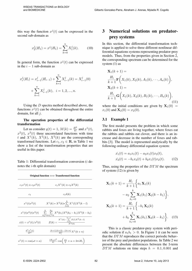
This is a classic predator-prey system with peri-odic solution if a1b1 > 0. In Figure 1 it can be seenthat the DTM reproduces the correct periodic behav-ior of the prey and predator populations. In Table 2 wepresent the absolute differences between the 3-termDTM solutions on time steps h = 0.1, 0.001 and



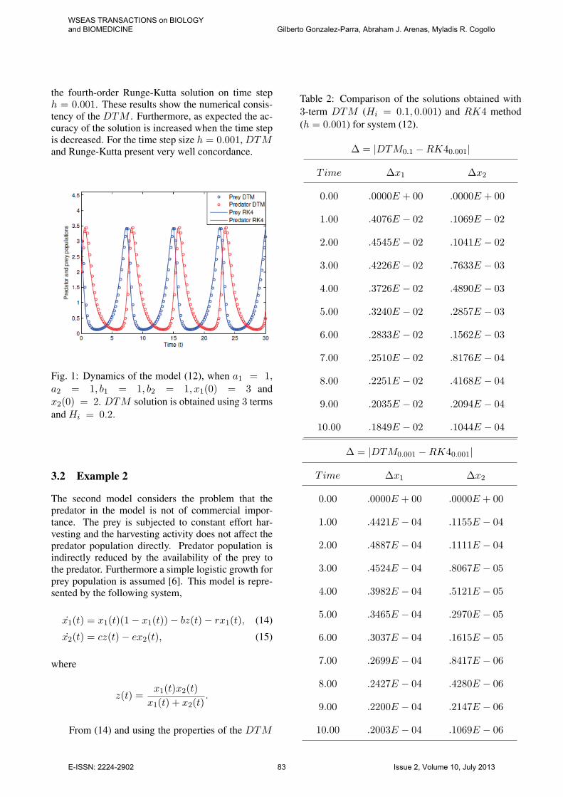
the fourth-order Runge-Kutta solution on time steph = 0.001. These results show the numerical consis-tency of the DTM . Furthermore, as expected the ac-curacy of the solution is increased when the time stepis decreased. For the time step size h = 0.001, DTMand Runge-Kutta present very well concordance.

Fig. 1: Dynamics of the model (12), when a1 = 1,a2 = 1, b1 = 1, b2 = 1, x1(0) = 3 andx2(0) = 2. DTM solution is obtained using 3 termsand Hi = 0.2.

3.2 Example 2

The second model considers the problem that thepredator in the model is not of commercial impor-tance. The prey is subjected to constant effort har-vesting and the harvesting activity does not affect thepredator population directly. Predator population isindirectly reduced by the availability of the prey tothe predator. Furthermore a simple logistic growth forprey population is assumed [6]. This model is repre-sented by the following system,

x1(t) = x1(t)(1− x1(t))− bz(t)− rx1(t), (14)

x2(t) = cz(t)− ex2(t), (15)

where

z(t) =x1(t)x2(t)

x1(t) + x2(t).

From (14) and using the properties of the DTM

Table 2: Comparison of the solutions obtained with3-term DTM (Hi = 0.1, 0.001) and RK4 method(h = 0.001) for system (12).

∆ = |DTM0.1 −RK40.001|

Time ∆x1 ∆x2

0.00 .0000E + 00 .0000E + 00

1.00 .4076E − 02 .1069E − 02

2.00 .4545E − 02 .1041E − 02

3.00 .4226E − 02 .7633E − 03

4.00 .3726E − 02 .4890E − 03

5.00 .3240E − 02 .2857E − 03

6.00 .2833E − 02 .1562E − 03

7.00 .2510E − 02 .8176E − 04

8.00 .2251E − 02 .4168E − 04

9.00 .2035E − 02 .2094E − 04

10.00 .1849E − 02 .1044E − 04

∆ = |DTM0.001 −RK40.001|

Time ∆x1 ∆x2

0.00 .0000E + 00 .0000E + 00

1.00 .4421E − 04 .1155E − 04

2.00 .4887E − 04 .1111E − 04

3.00 .4524E − 04 .8067E − 05

4.00 .3982E − 04 .5121E − 05

5.00 .3465E − 04 .2970E − 05

6.00 .3037E − 04 .1615E − 05

7.00 .2699E − 04 .8417E − 06

8.00 .2427E − 04 .4280E − 06

9.00 .2200E − 04 .2147E − 06

10.00 .2003E − 04 .1069E − 06



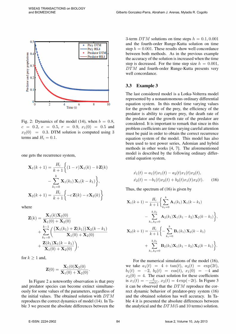
Fig. 2: Dynamics of the model (14), when b = 0.8,c = 0.2, e = 0.5, r = 0.9, x1(0) = 0.5 andx2(0) = 0.3. DTM solution is computed using 3terms and Hi = 0.1.

one gets the recurrence system,

X1(k + 1) =Hi

k + 1

{(1− r)X1(k)− bZ(k)

−k∑

k1=0

X1(k1)X1(k − k1)

},

X2(k + 1) =Hi

k + 1

{−cZ(k)− eX2(k)

}where

Z(k) =X1(k)X2(0)

X1(0) +X2(0)

+

k−1∑k1=0

((X1(k1) + Z(k1)

)X2(k − k1)

X1(0) +X2(0)

+Z(k1)X1(k − k1)

X1(0) +X2(0)

),

for k ≥ 1 and,

Z(0) =X1(0)X2(0)

X1(0) +X2(0).

In Figure 2 a noteworthy observation is that preyand predator species can become extinct simultane-ously for some values of the parameters, regardless ofthe initial values. The obtained solution with DTMreproduces the correct dynamics of model (14). In Ta-ble 3 we present the absolute differences between the

3-term DTM solutions on time steps h = 0.1, 0.001and the fourth-order Runge-Kutta solution on timestep h = 0.001. These results show well concordancebetween both methods. As in the previous examplethe accuracy of the solution is increased when the timestep is decreased. For the time step size h = 0.001,DTM and fourth-order Runge-Kutta presents verywell concordance.

3.3 Example 3

The last considered model is a Lotka-Volterra modelrepresented by a nonautonomous ordinary differentialequation system. In this model time varying valuesfor the growth rate of the prey, the efficiency of thepredator is ability to capture prey, the death rate ofthe predator and the growth rate of the predator areconsidered. It is important to remark that since in thisproblem coefficients are time varying careful attentionmust be paid in order to obtain the correct recurrenceequation system of the model. This model has alsobeen used to test power series, Adomian and hybridmethods in other works [4, 7]. The aforementionedmodel is described by the following ordinary differ-ential equation system,

x1(t) = a1(t)x1(t)− a2(t)x1(t)x2(t),

x2(t) = −b1(t)x2(t) + b2(t)x1(t)x2(t). (16)

Thus, the spectrum of (16) is given by

X1(k + 1) =Hi

k + 1

{ k∑k1=0

A1(k1)X1(k − k1)

−k,k1∑

k1,k2=0

A2(k1)X1(k1 − k2)X2(k − k1)

},

X2(k + 1) =Hi

k + 1

{−

k∑k1=0

B1(k1)X2(k − k1)

+

k,k1∑k1,k2=0

B2(k1)X1(k1 − k2)X2(k − k1)

}.

For the numerical simulations of the model (16),we take a1(t) = 4 + tan(t), a2(t) = exp(2t),b1(t) = −2, b2(t) = cos(t), x1(0) = −4 andx2(0) = 4. The exact solution for these coefficientsis x1(t) = − 4

cos(t) , x2(t) = 4 exp(−2t). In Figure 3it can be observed that the DTM reproduce the cor-rect dynamic behavior of predator-prey system (16)and the obtained solution has well accuracy. In Ta-ble 4 it is presented the absolute differences betweenthe analytical and the DTM (5 and 10 terms) solution.



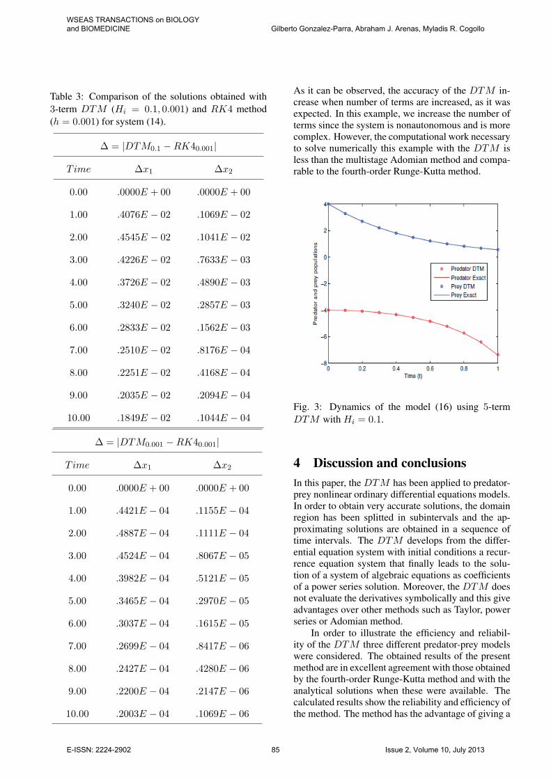
Table 3: Comparison of the solutions obtained with3-term DTM (Hi = 0.1, 0.001) and RK4 method(h = 0.001) for system (14).

∆ = |DTM0.1 −RK40.001|

Time ∆x1 ∆x2

0.00 .0000E + 00 .0000E + 00

1.00 .4076E − 02 .1069E − 02

2.00 .4545E − 02 .1041E − 02

3.00 .4226E − 02 .7633E − 03

4.00 .3726E − 02 .4890E − 03

5.00 .3240E − 02 .2857E − 03

6.00 .2833E − 02 .1562E − 03

7.00 .2510E − 02 .8176E − 04

8.00 .2251E − 02 .4168E − 04

9.00 .2035E − 02 .2094E − 04

10.00 .1849E − 02 .1044E − 04

∆ = |DTM0.001 −RK40.001|

Time ∆x1 ∆x2

0.00 .0000E + 00 .0000E + 00

1.00 .4421E − 04 .1155E − 04

2.00 .4887E − 04 .1111E − 04

3.00 .4524E − 04 .8067E − 05

4.00 .3982E − 04 .5121E − 05

5.00 .3465E − 04 .2970E − 05

6.00 .3037E − 04 .1615E − 05

7.00 .2699E − 04 .8417E − 06

8.00 .2427E − 04 .4280E − 06

9.00 .2200E − 04 .2147E − 06

10.00 .2003E − 04 .1069E − 06

As it can be observed, the accuracy of the DTM in-crease when number of terms are increased, as it wasexpected. In this example, we increase the number ofterms since the system is nonautonomous and is morecomplex. However, the computational work necessaryto solve numerically this example with the DTM isless than the multistage Adomian method and compa-rable to the fourth-order Runge-Kutta method.

Fig. 3: Dynamics of the model (16) using 5-termDTM with Hi = 0.1.

4 Discussion and conclusionsIn this paper, the DTM has been applied to predator-prey nonlinear ordinary differential equations models.In order to obtain very accurate solutions, the domainregion has been splitted in subintervals and the ap-proximating solutions are obtained in a sequence oftime intervals. The DTM develops from the differ-ential equation system with initial conditions a recur-rence equation system that finally leads to the solu-tion of a system of algebraic equations as coefficientsof a power series solution. Moreover, the DTM doesnot evaluate the derivatives symbolically and this giveadvantages over other methods such as Taylor, powerseries or Adomian method.

In order to illustrate the efficiency and reliabil-ity of the DTM three different predator-prey modelswere considered. The obtained results of the presentmethod are in excellent agreement with those obtainedby the fourth-order Runge-Kutta method and with theanalytical solutions when these were available. Thecalculated results show the reliability and efficiency ofthe method. The method has the advantage of giving a



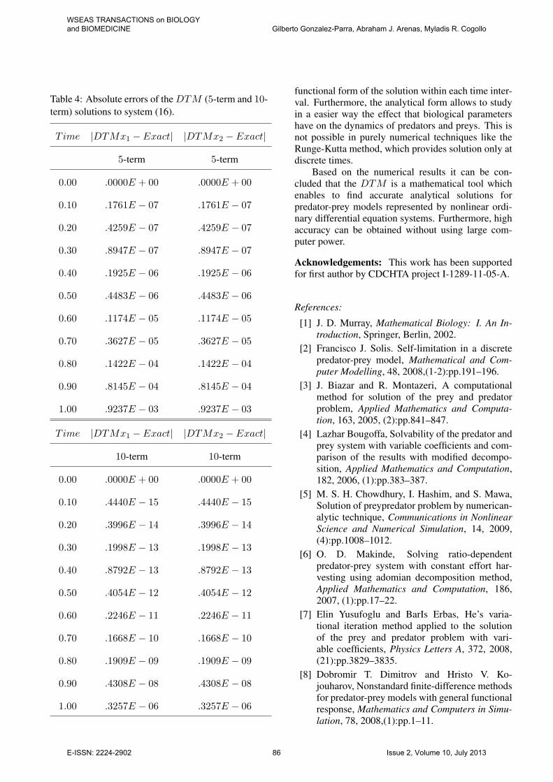
Table 4: Absolute errors of the DTM (5-term and 10-term) solutions to system (16).

Time |DTMx1 − Exact| |DTMx2 − Exact|

5-term 5-term

0.00 .0000E + 00 .0000E + 00

0.10 .1761E − 07 .1761E − 07

0.20 .4259E − 07 .4259E − 07

0.30 .8947E − 07 .8947E − 07

0.40 .1925E − 06 .1925E − 06

0.50 .4483E − 06 .4483E − 06

0.60 .1174E − 05 .1174E − 05

0.70 .3627E − 05 .3627E − 05

0.80 .1422E − 04 .1422E − 04

0.90 .8145E − 04 .8145E − 04

1.00 .9237E − 03 .9237E − 03

Time |DTMx1 − Exact| |DTMx2 − Exact|

10-term 10-term

0.00 .0000E + 00 .0000E + 00

0.10 .4440E − 15 .4440E − 15

0.20 .3996E − 14 .3996E − 14

0.30 .1998E − 13 .1998E − 13

0.40 .8792E − 13 .8792E − 13

0.50 .4054E − 12 .4054E − 12

0.60 .2246E − 11 .2246E − 11

0.70 .1668E − 10 .1668E − 10

0.80 .1909E − 09 .1909E − 09

0.90 .4308E − 08 .4308E − 08

1.00 .3257E − 06 .3257E − 06

functional form of the solution within each time inter-val. Furthermore, the analytical form allows to studyin a easier way the effect that biological parametershave on the dynamics of predators and preys. This isnot possible in purely numerical techniques like theRunge-Kutta method, which provides solution only atdiscrete times.

Based on the numerical results it can be con-cluded that the DTM is a mathematical tool whichenables to find accurate analytical solutions forpredator-prey models represented by nonlinear ordi-nary differential equation systems. Furthermore, highaccuracy can be obtained without using large com-puter power.

Acknowledgements: This work has been supportedfor first author by CDCHTA project I-1289-11-05-A.

References:

[1] J. D. Murray, Mathematical Biology: I. An In-troduction, Springer, Berlin, 2002.

[2] Francisco J. Solis. Self-limitation in a discretepredator-prey model, Mathematical and Com-puter Modelling, 48, 2008,(1-2):pp.191–196.

[3] J. Biazar and R. Montazeri, A computationalmethod for solution of the prey and predatorproblem, Applied Mathematics and Computa-tion, 163, 2005, (2):pp.841–847.

[4] Lazhar Bougoffa, Solvability of the predator andprey system with variable coefficients and com-parison of the results with modified decompo-sition, Applied Mathematics and Computation,182, 2006, (1):pp.383–387.

[5] M. S. H. Chowdhury, I. Hashim, and S. Mawa,Solution of preypredator problem by numerican-alytic technique, Communications in NonlinearScience and Numerical Simulation, 14, 2009,(4):pp.1008–1012.

[6] O. D. Makinde, Solving ratio-dependentpredator-prey system with constant effort har-vesting using adomian decomposition method,Applied Mathematics and Computation, 186,2007, (1):pp.17–22.

[7] Elin Yusufoglu and BarIs Erbas, He’s varia-tional iteration method applied to the solutionof the prey and predator problem with vari-able coefficients, Physics Letters A, 372, 2008,(21):pp.3829–3835.

[8] Dobromir T. Dimitrov and Hristo V. Ko-jouharov, Nonstandard finite-difference methodsfor predator-prey models with general functionalresponse, Mathematics and Computers in Simu-lation, 78, 2008,(1):pp.1–11.



[9] Vedat Suat Erturk and Shaher Momani, Solu-tions to the problem of prey and predator andthe epidemic model via differential transformmethod, Kybernetes, 37, 2008, (8):pp.1180–1188.

[10] J. K. Zhou, Differential Transformation and itsApplications for Electrical Circuits, HuazhongUniversity Press, Wuhan,(in Chinese), 1986.

[11] M. Mossa Al-Sawalha and M. S. M. Noorani,Application of the differential transformationmethod for the solution of the hyper chaoticRssler system, Communications in NonlinearScience and Numerical Simulation, 14, 2009,(4):pp.1509–1514.

[12] A. J. Arenas, G. Gonzalez-Parra, and B. M.Chen- Charpentier, Dynamical analysis of thetransmission of seasonal diseases using the dif-ferential transformation method, Mathematicaland Computer Modelling, 50, 2009,(5):pp.765–776.

[13] Shih-Shin Chen and Chao-Kuang Chen, Appli-cation of the differential transformation methodto the free vibrations of strongly non-linear os-cillators, Nonlinear Analysis: Real World Appli-cations, 10, 2009, (2):pp.881–888.

[14] Hsin-Ping Chu and Chieh-Li Chen, Hybrid dif-ferential transform and finite difference methodto solve the nonlinear heat conduction prob-lem, Communications in Nonlinear Science andNumerical Simulation, 13, 2008, (8):pp.1605–1614.

[15] G. Gonzalez-Parra, L. Acedo, and A. Arenas,Accuracy of analytical-numerical solutions ofthe michaelis-menten equation,Computational& Applied Mathematics, 30, 2011, (2):pp.445–461.

[16] A. Ebaid, On a general formula for comput-ing the one-dimensional differential transform ofnonlinear functions and its applications, In Pro-ceedings of the 6th WSEAS international con-ference on Computer Engineering and Applica-tions, and Proceedings of the 2012 Americanconference on Applied Mathematics, pages 92–97. World Scientific and Engineering Academyand Society (WSEAS), 2012.

[17] M. T. Kajani and N. A. Shehni, Solutions of two-dimensional integral equation systems by usingdifferential transform method, In Proceedings ofthe 2011 American conference on applied math-ematics and the 5th WSEAS international con-ference on Computer engineering and applica-tions, pages 74–77. World Scientific and Engi-neering Academy and Society (WSEAS), 2011.

[18] L. Villafuerte and B. M. Chen-Charpentier, Arandom differential transform method: Theoryand applications, Applied Mathematics Letters,25, 2012,(10):pp.1490–1494.

[19] J. A. Licea, L. Villafuerte, and B. M. Chen-Charpentier, Analytic and numerical solutions ofa riccati differential equation with random coef-ficients, Journal of Computational and AppliedMathematics, 239, 2013, pp.208–219.

[20] Abraham J. Arenas, Gilberto Gonzalez-Parra,Lucas Jodar, and Rafael-J. Villanueva. Piecewisefinite series solution of nonlinear initial valuedifferential problem, Applied Mathematics andComputation, 212, 2009, (1):pp. 209–215,



Documents

Numerical-analytical solutions of predator-prey … solutions of predator-prey models GILBERTO GONZALEZ-PARRA´ Grupo de Matem´atica Multidisciplinar (GMM) Dpto. Calculo, Facultad