Proceedings of 8th PAAMES and AMEC 2018 9-12 October 2018, Busan

Numerical Analysis of Propulsion for Submarine with Highly Skewed Propeller

Yung-An Chu1, Chun-Ta Lin1, Ching-Yeh Hsin2, Ya-Jung Lee3

1 R/D Section, Research Department, CR Classification Society, Taipei, Taiwan 10491

2 Dept. of Systems Engineering and Naval Architecture, National Taiwan Ocean University, Taiwan 20224

3 Dept. of Engineering Science and Ocean Engineering, National Taiwan University, Taiwan 10617

Abstract Propulsion simulation of an axisymmetric submerged body in RANS coupled with propeller body force method is

presented. The calm water resistance of DARPA SUBOFF model with full appendages was calculated by CFD software.

A generic submarine propeller based on INSEAN E1619 was constructed to the published projected outlines and specific

pitch at 70% radial position to match the experimental open water K-J chart, especially the thrust coefficient among the

whole operational range. A 3D panel method of potential flow solver was utilized to calculate propeller performance, as

well as providing the equivalent body forces for propulsion simulation. Comprehensive wake survey were carried out and

compared with virtual disk model. The effect of various propeller loading conditions on the propulsive characteristics of

the submarine model was investigated. The results of the body force approach with panel method show better agreement

with other fully RANS simulation.

Keywords: Propulsion, Submarine, Body force, RANS

1. Introduction In regards of underwater noise, submarines are com-

monly equipped with a highly skewed propeller. For such

kind of geometry, the model and a suitable body-fitted

grid in RANS will take a long time to build, so that decel-

erating the design process.

Huang and Groves compared the effect of interac-

tion between the axisymmetric body and propeller

through experimental approaches and calculating the

asymmetric Euler equations, which gave precise pre-

dictions of the thrust deduction and the pressure dis-

tribution induced by the operating propeller. For

analysis of the interaction between the wake and pro-

peller, direct calculating the ship along with its pro-

peller using viscous flow RANS model is the most

intuitive way. However, due to the highly compli-

cated geometry of the propeller, the need to use enor-

mous grid numbers to resolve the flow near the pro-

peller made the way impractical to conduct, let alone

the necessity of using unsteady flow calculation.

Therefore, potential flow is the most effective and

efficient to calculate the propeller force, and makes

both flow fields coupled with each other well.

Wei(2012) numerically simulated the self propulsion

of the surface ship by CFD method coupled with

Body Force Method. Estimations of the self propul-

sion point showed a good agreement with the that of

experiment method. Chase(2012) carried out a series

of investigation for the DARPA SUBOFF model, in-

cluding the simulations of the self-propulsion condi-

tion with INSEAN E1619 by using the overset flow

solver CFDShip-Iowa V4.5. Sinan(2017) also used

the same submarine and propeller model with AN-

SYS Fluent. Computations are validated by the pub-

lished experimental data of the propeller for forward

speed and forward propeller rotation and the rest of

the quadrants are predicted numerically.

In the study, a variety of tests have been simulated

by CFD method and 3D panel method of potential

flow solver. Validation and comparison using differ-

ent methods are presented.

2. Geometry Models Details of the submarine model and propeller

model used in the study are as follows:

2.1 Submarine model

Among the submarine model for the academic

purpose, the DARPA SUBOFF model is the most

commonly used due to a great deal of available ex-

periment data and extensive researches for valida-

tion and comparison (Liu and Huang, 1998). In the

study, the AFF-8 configuration including the fair-

water, and stern rudders is chose for simulation. It

comprises of a fairwater which is located at the top

dead center of the hull starting at x = 0.92 m from

the bow and ending at x = 1.29 m as well as a cross

shaped rudder where rudders and hydroplanes are lo-

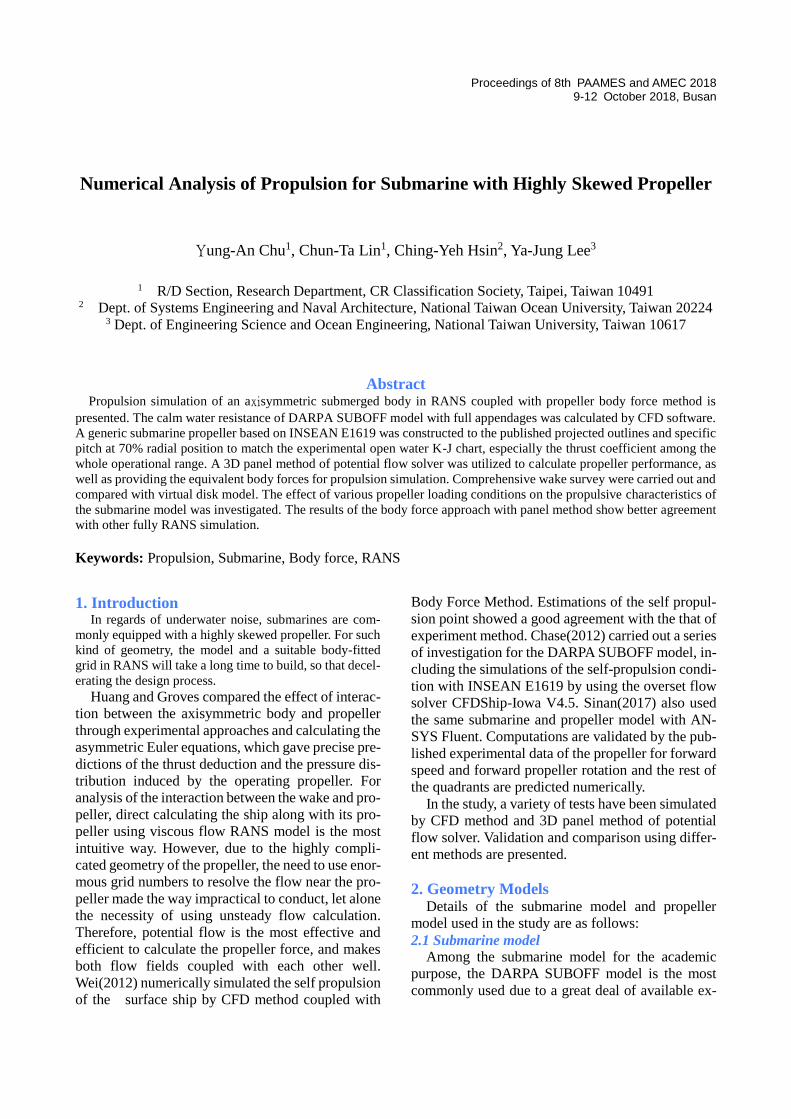
cated at x=4 m from the bow. The main dimensions

of the computational domain are determined in ac-

cordance with the ITTC guidelines. Top view and

side view of the computational domain and are given

in Figure 1. Mesh of the whole computational do-

main was displayed in Figure 2.

Table 1 Principal particulars of DARPA SUBOFF

Description Symbol Magnitude

Length overall LOA 4.356 m

Length between per-

penticulars

Lpp 4.261 m

Maximum hull radius Rmax 0.254 m

Centre of buoyancy

(aft of nose)

FB 0.4621 LOA

Volume of displace-

ment

0.718 m3

Wetted Surface Sw 6.338 m2

Propeller Diameter PD 0.262 m

Fig. 1 Computational domain of DARPA SUBOFF

Fig. 2 Cut-away view of DARPA SUBOFF

2.2 Propeller Model

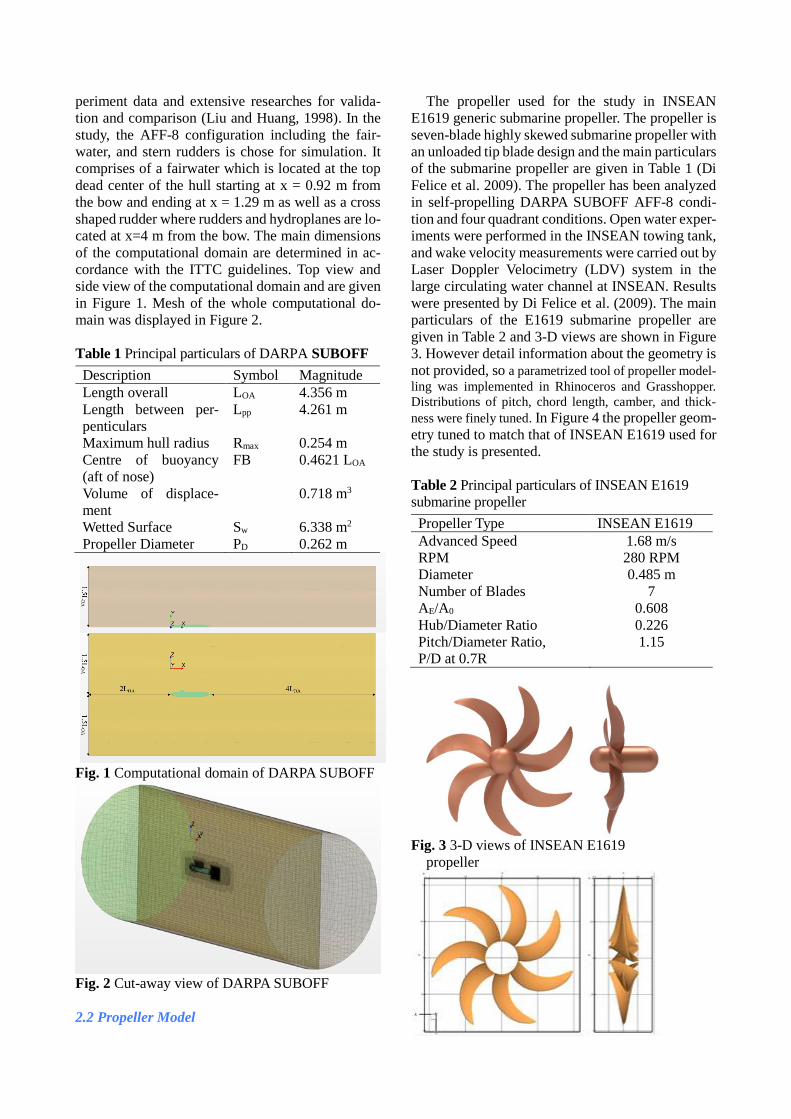
The propeller used for the study in INSEAN

E1619 generic submarine propeller. The propeller is

seven-blade highly skewed submarine propeller with

an unloaded tip blade design and the main particulars

of the submarine propeller are given in Table 1 (Di

Felice et al. 2009). The propeller has been analyzed

in self-propelling DARPA SUBOFF AFF-8 condi-

tion and four quadrant conditions. Open water exper-

iments were performed in the INSEAN towing tank,

and wake velocity measurements were carried out by

Laser Doppler Velocimetry (LDV) system in the

large circulating water channel at INSEAN. Results

were presented by Di Felice et al. (2009). The main

particulars of the E1619 submarine propeller are

given in Table 2 and 3-D views are shown in Figure

3. However detail information about the geometry is

not provided, so a parametrized tool of propeller model-

ling was implemented in Rhinoceros and Grasshopper.

Distributions of pitch, chord length, camber, and thick-

ness were finely tuned. In Figure 4 the propeller geom-

etry tuned to match that of INSEAN E1619 used for

the study is presented.

Table 2 Principal particulars of INSEAN E1619

submarine propeller

Propeller Type INSEAN E1619

Advanced Speed 1.68 m/s

RPM 280 RPM

Diameter 0.485 m

Number of Blades 7

AE/A0 0.608

Hub/Diameter Ratio 0.226

Pitch/Diameter Ratio,

P/D at 0.7R

1.15

Fig. 3 3-D views of INSEAN E1619

propeller

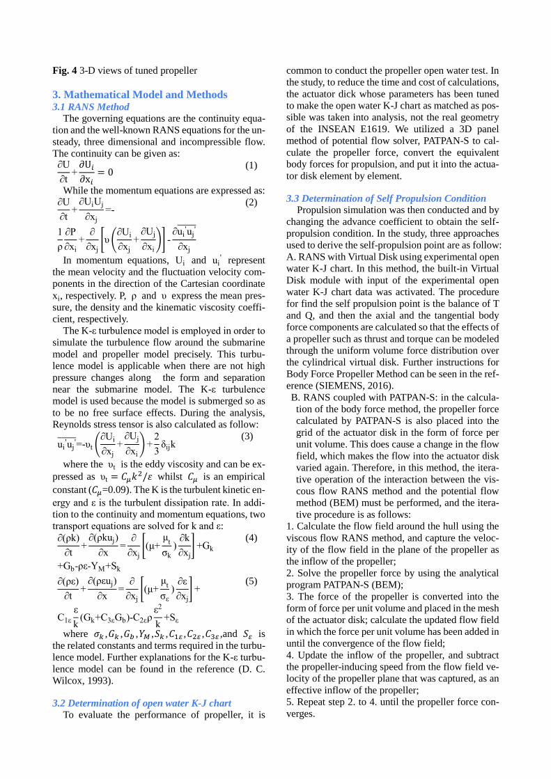
Fig. 4 3-D views of tuned propeller

3. Mathematical Model and Methods 3.1 RANS Method

The governing equations are the continuity equa-

tion and the well-known RANS equations for the un-

steady, three dimensional and incompressible flow.

The continuity can be given as: ∂U

∂t+∂U𝑖∂x𝑖

= 0 (1)

While the momentum equations are expressed as: ∂U

∂t+

∂UiUj

∂xj

=-

1

ρ

∂P

∂xi

+∂

∂xj

[υ(∂Ui

∂xj

+∂Uj

∂xi

)] -∂ui

'uj'̅̅ ̅̅ ̅̅

∂xj

(2)

In momentum equations, Ui and ui' represent

the mean velocity and the fluctuation velocity com-

ponents in the direction of the Cartesian coordinate

xi, respectively. P, ρ and υ express the mean pres-

sure, the density and the kinematic viscosity coeffi-

cient, respectively.

The K-ε turbulence model is employed in order to

simulate the turbulence flow around the submarine

model and propeller model precisely. This turbu-

lence model is applicable when there are not high

pressure changes along the form and separation

near the submarine model. The K-ε turbulence

model is used because the model is submerged so as

to be no free surface effects. During the analysis,

Reynolds stress tensor is also calculated as follow:

ui'uj

'̅̅ ̅̅ ̅̅ =-υt (∂Ui

∂xj

+∂Uj

∂xi

)+2

3δijk

(3)

where the υt is the eddy viscosity and can be ex-

pressed as υt = 𝐶𝜇𝑘2/𝜀 whilst 𝐶𝜇 is an empirical

constant (𝐶𝜇=0.09). The K is the turbulent kinetic en-

ergy and ε is the turbulent dissipation rate. In addi-

tion to the continuity and momentum equations, two

transport equations are solved for k and ε:

∂(ρk)

∂t+

∂(ρkuj)

∂x=

∂

∂xj

[(μ+μ

t

σk

)∂k

∂xj

]+Gk

+Gb-ρε-YM+Sk

(4)

∂(ρε)

∂t+

∂(ρεuj)

∂x=

∂

∂xj

[(μ+μ

t

σε

)∂ε

∂xj

]+

C1ε

ε

k(Gk+C3εGb)-C2ερ

ε2

k+Sε

(5)

where 𝜎𝑘 ,𝐺𝑘 ,𝐺𝑏 ,𝑌𝑀 ,𝑆𝑘 ,𝐶1𝜀 ,𝐶2𝜀 ,𝐶3𝜀 ,and 𝑆𝜀 is

the related constants and terms required in the turbu-

lence model. Further explanations for the K-ε turbu-

lence model can be found in the reference (D. C.

Wilcox, 1993).

3.2 Determination of open water K-J chart

To evaluate the performance of propeller, it is

common to conduct the propeller open water test. In

the study, to reduce the time and cost of calculations,

the actuator dick whose parameters has been tuned

to make the open water K-J chart as matched as pos-

sible was taken into analysis, not the real geometry

of the INSEAN E1619. We utilized a 3D panel

method of potential flow solver, PATPAN-S to cal-

culate the propeller force, convert the equivalent

body forces for propulsion, and put it into the actua-

tor disk element by element.

3.3 Determination of Self Propulsion Condition

Propulsion simulation was then conducted and by

changing the advance coefficient to obtain the self-

propulsion condition. In the study, three approaches

used to derive the self-propulsion point are as follow:

A. RANS with Virtual Disk using experimental open

water K-J chart. In this method, the built-in Virtual

Disk module with input of the experimental open

water K-J chart data was activated. The procedure

for find the self propulsion point is the balance of T

and Q, and then the axial and the tangential body

force components are calculated so that the effects of

a propeller such as thrust and torque can be modeled

through the uniform volume force distribution over

the cylindrical virtual disk. Further instructions for

Body Force Propeller Method can be seen in the ref-

erence (SIEMENS, 2016).

B. RANS coupled with PATPAN-S: in the calcula-

tion of the body force method, the propeller force

calculated by PATPAN-S is also placed into the

grid of the actuator disk in the form of force per

unit volume. This does cause a change in the flow

field, which makes the flow into the actuator disk

varied again. Therefore, in this method, the itera-

tive operation of the interaction between the vis-

cous flow RANS method and the potential flow

method (BEM) must be performed, and the itera-

tive procedure is as follows:

1. Calculate the flow field around the hull using the

viscous flow RANS method, and capture the veloc-

ity of the flow field in the plane of the propeller as

the inflow of the propeller;

2. Solve the propeller force by using the analytical

program PATPAN-S (BEM);

3. The force of the propeller is converted into the

form of force per unit volume and placed in the mesh

of the actuator disk; calculate the updated flow field

in which the force per unit volume has been added in

until the convergence of the flow field;

4. Update the inflow of the propeller, and subtract

the propeller-inducing speed from the flow field ve-

locity of the propeller plane that was captured, as an

effective inflow of the propeller;

5. Repeat step 2. to 4. until the propeller force con-

verges.

C. RANS with Virtual Disk using open water K-J

chart of the tuned propeller: open water K-J chart

of the tuned propeller has been input in the CFD

software with Virtual Disk module activated.

4. Results Three traditional tests in the naval architecture

have been simulated and elaborated as follows:

4.1 Resistance Test

Assumption was made that the submarine model

advanced in the infinite calm water so that free sur-

face effect on the total resistance of the model was

neglected. Structured mesh was generated in the

whole computational domain and refinement was

made where the curvature of the hull varied dramat-

ically as well as the geometric continuity failed to be

retained. Also, grid sensitivity for both the minimum

and maximum tested speed as shown in Figure 6 and

Figure 7 was conduct to ensure the sufficient grid

numbers were produced before a series of resistance

simulations were executed. The final grid number

was about 13.5 million. The appropriate boundary

condition could facilitate the convergence of the

flow. In this part, because of the bilateral symmetry

of the submarine model, half of the form was created

to simplify the problem and reduce the time of anal-

ysis. Hence, the boundary conditions in the part are

shown in Figure 4.

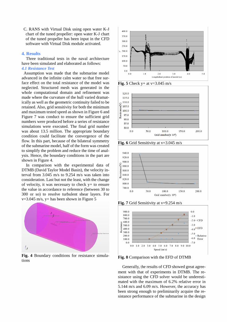
In comparison with the experimental data of

DTMB (David Taylor Model Basin), the velocity in-

terval from 3.045 m/s to 9.254 m/s was taken into

consideration. Last but not the least, with the change

of velocity, it was necessary to check y+ to ensure

the value in accordance to reference (between 30 to

300 or so) to resolve turbulent shear layers. For

v=3.045 m/s, y+ has been shown in Figure 5

Fig. 4 Boundary conditions for resistance simula-

tions

Fig. 5 Check y+ at v=3.045 m/s

Fig. 6 Grid Sensitivity at v=3.045 m/s

Fig. 7 Grid Sensitivity at v=9.254 m/s

Fig. 8 Comparison with the EFD of DTMB

Generally, the results of CFD showed great agree-

ment with that of experiments in DTMB. The re-

sistance using the CFD solver would be underesti-

mated with the maximum of 6.2% relative error in

5.144 m/s and 6.09 m/s. However, the accuracy has

been strong enough to preliminarily acquire the re-

sistance performance of the submarine in the design

stage.

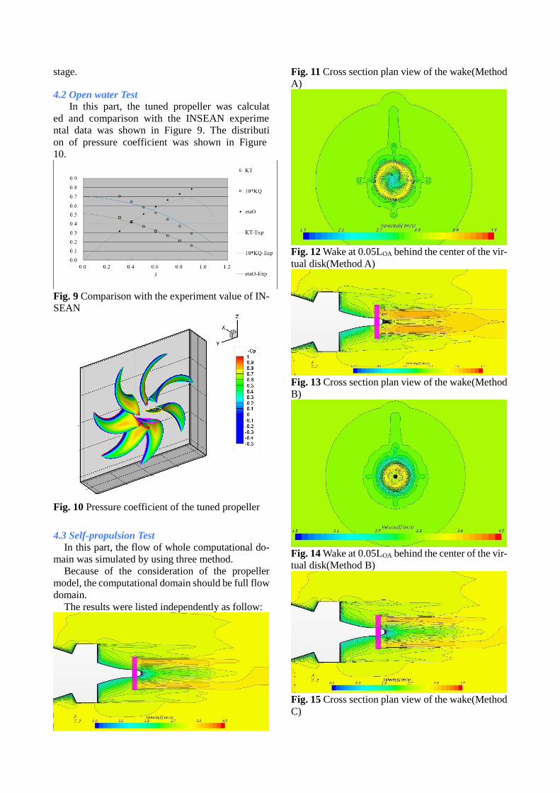
4.2 Open water Test

In this part, the tuned propeller was calculat

ed and comparison with the INSEAN experime

ntal data was shown in Figure 9. The distributi

on of pressure coefficient was shown in Figure

10.

Fig. 9 Comparison with the experiment value of IN-

SEAN

Fig. 10 Pressure coefficient of the tuned propeller

4.3 Self-propulsion Test

In this part, the flow of whole computational do-

main was simulated by using three method.

Because of the consideration of the propeller

model, the computational domain should be full flow

domain.

The results were listed independently as follow:

Fig. 11 Cross section plan view of the wake(Method

A)

Fig. 12 Wake at 0.05LOA behind the center of the vir-

tual disk(Method A)

Fig. 13 Cross section plan view of the wake(Method

B)

Fig. 14 Wake at 0.05LOA behind the center of the vir-

tual disk(Method B)

Fig. 15 Cross section plan view of the wake(Method

C)

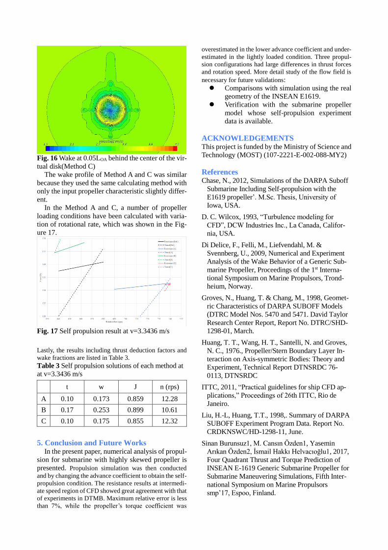
Fig. 16 Wake at 0.05LOA behind the center of the vir-

tual disk(Method C)

The wake profile of Method A and C was similar

because they used the same calculating method with

only the input propeller characteristic slightly differ-

ent.

In the Method A and C, a number of propeller

loading conditions have been calculated with varia-

tion of rotational rate, which was shown in the Fig-

ure 17.

Fig. 17 Self propulsion result at v=3.3436 m/s

Lastly, the results including thrust deduction factors and

wake fractions are listed in Table 3.

Table 3 Self propulsion solutions of each method at

at v=3.3436 m/s

t w J n (rps)

A 0.10 0.173 0.859 12.28

B 0.17 0.253 0.899 10.61

C 0.10 0.175 0.855 12.32

5. Conclusion and Future Works In the present paper, numerical analysis of propul-

sion for submarine with highly skewed propeller is

presented. Propulsion simulation was then conducted

and by changing the advance coefficient to obtain the self-

propulsion condition. The resistance results at intermedi-

ate speed region of CFD showed great agreement with that

of experiments in DTMB. Maximum relative error is less

than 7%, while the propeller’s torque coefficient was

overestimated in the lower advance coefficient and under-

estimated in the lightly loaded condition. Three propul-

sion configurations had large differences in thrust forces

and rotation speed. More detail study of the flow field is

necessary for future validations:

Comparisons with simulation using the real

geometry of the INSEAN E1619.

Verification with the submarine propeller

model whose self-propulsion experiment

data is available.

ACKNOWLEDGEMENTS This project is funded by the Ministry of Science and

Technology (MOST) (107-2221-E-002-088-MY2)

References Chase, N., 2012, Simulations of the DARPA Suboff

Submarine Including Self-propulsion with the

E1619 propeller’. M.Sc. Thesis, University of

Iowa, USA.

D. C. Wilcox, 1993, “Turbulence modeling for

CFD”, DCW Industries Inc., La Canada, Califor-

nia, USA.

Di Delice, F., Felli, M., Liefvendahl, M. &

Svennberg, U., 2009, Numerical and Experiment

Analysis of the Wake Behavior of a Generic Sub-

marine Propeller, Proceedings of the 1st Interna-

tional Symposium on Marine Propulsors, Trond-

heium, Norway.

Groves, N., Huang, T. & Chang, M., 1998, Geomet-

ric Characteristics of DARPA SUBOFF Models

(DTRC Model Nos. 5470 and 5471. David Taylor

Research Center Report, Report No. DTRC/SHD-

1298-01, March.

Huang, T. T., Wang, H. T., Santelli, N. and Groves,

N. C., 1976., Propeller/Stern Boundary Layer In-

teraction on Axis-symmetric Bodies: Theory and

Experiment, Technical Report DTNSRDC 76-

0113, DTNSRDC

ITTC, 2011, “Practical guidelines for ship CFD ap-

plications,” Proceedings of 26th ITTC, Rio de

Janeiro.

Liu, H.-L, Huang, T.T., 1998,. Summary of DARPA

SUBOFF Experiment Program Data. Report No.

CRDKNSWC/HD-1298-11, June.

Sinan Burunsuz1, M. Cansın Özden1, Yasemin

Arıkan Özden2, İsmail Hakkı Helvacıoğlu1, 2017,

Four Quadrant Thrust and Torque Prediction of

INSEAN E-1619 Generic Submarine Propeller for

Submarine Maneuvering Simulations, Fifth Inter-

national Symposium on Marine Propulsors

smp’17, Espoo, Finland.

Y. Cengel and J. M. Cimbalak, 2008, Essentials of

fluid mechanics: fundamentals and applications,

McGraw-Hill Higher Education.

SIEMENS, 2006, STAR-CCM+ v11.06Theory

Guide